# Table of Contents
- [SATLAS2 – Statistical Analysis Toolbox for Laser Spectroscopy, version 2 — SATLAS2](#satlas2-statistical-analysis-toolbox-for-laser-spectroscopy-version-2-satlas2)
- [Unknown](#unknown)
- [Architecture of SATLAS2 — SATLAS2](#architecture-of-satlas2-satlas2)
- [Tutorial — SATLAS2](#tutorial-satlas2)
- [Unknown](#unknown)
- [Fitting in SATLAS2 — SATLAS2](#fitting-in-satlas2-satlas2)
- [Unknown](#unknown)
- [Making a model — SATLAS2](#making-a-model-satlas2)
- [Extracting dataframes — SATLAS2](#extracting-dataframes-satlas2)
- [Different emcee moves — SATLAS2](#different-emcee-moves-satlas2)
- [Benchmark of SATLAS2 speed — SATLAS2](#benchmark-of-satlas2-speed-satlas2)
- [Unknown](#unknown)
- [API reference — SATLAS2](#api-reference-satlas2)
- [Using the SATLAS interface — SATLAS2](#using-the-satlas-interface-satlas2)
- [Unknown](#unknown)
- [Unknown](#unknown)
- [Unknown](#unknown)
- [Unknown](#unknown)
- [Python Module Index — SATLAS2](#python-module-index-satlas2)
- [Index — SATLAS2](#index-satlas2)
- [Search - SATLAS2](#search-satlas2)
- [API Models — SATLAS2](#api-models-satlas2)
- [API Core — SATLAS2](#api-core-satlas2)
- [Unknown](#unknown)
- [API Interface — SATLAS2](#api-interface-satlas2)
- [API Plotting — SATLAS2](#api-plotting-satlas2)
- [API Utilities — SATLAS2](#api-utilities-satlas2)
- [Unknown](#unknown)
- [Unknown](#unknown)
- [Unknown](#unknown)
- [Unknown](#unknown)
- [Unknown](#unknown)
- [Unknown](#unknown)
---
# SATLAS2 – Statistical Analysis Toolbox for Laser Spectroscopy, version 2 — SATLAS2
[Skip to main content](https://iks-nm.github.io/satlas2/index.html#main-content)
Back to top Ctrl+K
[ \
\
SATLAS2](https://iks-nm.github.io/satlas2/index.html#)
Search Ctrl+K
* [Repository](https://github.com/iks-nm/satlas2)
* [Suggest edit](https://github.com/iks-nm/satlas2/edit/master/index.rst)
* [Open issue](https://github.com/iks-nm/satlas2/issues/new?title=Issue%20on%20page%20%2Findex.html&body=Your%20issue%20content%20here.)
* [.rst](https://iks-nm.github.io/satlas2/_sources/index.rst)
* .pdf
Light Dark System Settings
SATLAS2 – Statistical Analysis Toolbox for Laser Spectroscopy, version 2
========================================================================
Contents
--------
SATLAS2 – Statistical Analysis Toolbox for Laser Spectroscopy, version 2[#](https://iks-nm.github.io/satlas2/index.html#satlas2-statistical-analysis-toolbox-for-laser-spectroscopy-version-2 "Permalink to this heading")
===========================================================================================================================================================================================================================
  


[](https://doi.org/10.1016/j.cpc.2023.109053)
Purpose[#](https://iks-nm.github.io/satlas2/index.html#purpose "Permalink to this heading")
============================================================================================
This Python package has been created with the goal of creating an easier interface for the analysis of data gathered from laser spectroscopy experiments. Support for fitting the spectra, using both χ2\-fitting and Maximum Likelihood Estimation routines, are present.
Dependencies[#](https://iks-nm.github.io/satlas2/index.html#dependencies "Permalink to this heading")
======================================================================================================
This package has the following dependencies:
> * [NumPy](http://www.numpy.org/)
>
> * [Matplotlib](http://matplotlib.org/)
>
> * [SciPy](http://www.scipy.org/)
>
> * [h5py](http://docs.h5py.org/en/latest/index.html)
>
> * [emcee](http://dan.iel.fm/emcee/current/)
>
> * [sympy](http://www.sympy.org/)
>
> * [LMFIT](http://lmfit.github.io/lmfit-py/index.html)
>
> * [numdifftools](http://numdifftools.readthedocs.io/en/latest/)
>
> * [uncertainties](https://pythonhosted.org/uncertainties/)
>
> * [tqdm](https://github.com/tqdm/tqdm)
>
> * [pandas](https://pandas.pydata.org/)
>
Contents[#](https://iks-nm.github.io/satlas2/index.html#contents "Permalink to this heading")
==============================================================================================
* [Architecture of SATLAS2](https://iks-nm.github.io/satlas2/architecture/index.html)
* [Tutorial](https://iks-nm.github.io/satlas2/tutorials/index.html)
* [API reference](https://iks-nm.github.io/satlas2/api/index.html)
Indices and tables[#](https://iks-nm.github.io/satlas2/index.html#indices-and-tables "Permalink to this heading")
==================================================================================================================
* [Index](https://iks-nm.github.io/satlas2/genindex.html)
* [Module Index](https://iks-nm.github.io/satlas2/py-modindex.html)
* [Search Page](https://iks-nm.github.io/satlas2/search.html)
Contents
---
# Unknown
SATLAS2 -- Statistical Analysis Toolbox for Laser Spectroscopy, version 2 ========================================================================= .. image:: https://img.shields.io/pypi/v/satlas2?label=PyPI%20version :alt: PyPI .. image:: https://img.shields.io/pypi/pyversions/satlas2?label=Python%20version&logo=python&logoColor=white :alt: PyPI - Python Version .. image:: https://img.shields.io/pypi/l/satlas2?color=blue&label=License :alt: PyPI - License \\ .. image:: https://img.shields.io/badge/Tested\_on-Windows/Linux-green.svg :alt: Supported Platform .. image:: https://img.shields.io/badge/Not\_tested\_on-Mac-red.svg :alt: Unsupported platform \\ .. image:: https://img.shields.io/pypi/dm/satlas2?label=Downloads :alt: PyPI - Downloads \\ .. image:: https://img.shields.io/badge/DOI-https%3A%2F%2Fdoi.org%2F10.1016%2Fj.cpc.2023.109053-blue :target: https://doi.org/10.1016/j.cpc.2023.109053 Purpose ======= .. sidebar:: Contributors - Bram van den Borne - Wouter Gins This Python package has been created with the goal of creating an easier interface for the analysis of data gathered from laser spectroscopy experiments. Support for fitting the spectra, using both :math:\`\\chi^2\`-fitting and Maximum Likelihood Estimation routines, are present. Dependencies ============ This package has the following dependencies: \* \`NumPy \`\_ \* \`Matplotlib \`\_ \* \`SciPy \`\_ \* \`h5py \`\_ \* \`emcee \`\_ \* \`sympy \`\_ \* \`LMFIT \`\_ \* \`numdifftools \`\_ \* \`uncertainties \`\_ \* \`tqdm \`\_ \* \`pandas \`\_ Contents ======== .. toctree:: :maxdepth: 1 architecture/index tutorials/index api/index Indices and tables ================== \* :ref:\`genindex\` \* :ref:\`modindex\` \* :ref:\`search\`
---
# Architecture of SATLAS2 — SATLAS2
[Skip to main content](https://iks-nm.github.io/satlas2/architecture/index.html#main-content)
Back to top Ctrl+K
[ \
\
SATLAS2](https://iks-nm.github.io/satlas2/index.html)
Search Ctrl+K
* [Repository](https://github.com/iks-nm/satlas2)
* [Suggest edit](https://github.com/iks-nm/satlas2/edit/master/architecture/index.rst)
* [Open issue](https://github.com/iks-nm/satlas2/issues/new?title=Issue%20on%20page%20%2Farchitecture/index.html&body=Your%20issue%20content%20here.)
* [.rst](https://iks-nm.github.io/satlas2/_sources/architecture/index.rst)
* .pdf
Light Dark System Settings
Architecture of SATLAS2
=======================
Architecture of SATLAS2[#](https://iks-nm.github.io/satlas2/architecture/index.html#architecture-of-satlas2 "Permalink to this heading")
=========================================================================================================================================
The SATLAS2 architecture has been streamlined and differs enormously from SATLAS. For a way to mostly reuse old SATLAS code, see the [interface tutorial](https://iks-nm.github.io/satlas2/tutorials/interface/index.html)
. Help
In SATLAS2, the main object to work with is the [`Fitter`](https://iks-nm.github.io/satlas2/api/summaries/core.html#satlas2.core.Fitter "satlas2.core.Fitter")
object. This object can be assigned one or more [`Source`](https://iks-nm.github.io/satlas2/api/summaries/core.html#satlas2.core.Source "satlas2.core.Source")
objects through the [`addSource`](https://iks-nm.github.io/satlas2/api/summaries/core.html#satlas2.core.Fitter.addSource "satlas2.core.Fitter.addSource")
method. This [`Source`](https://iks-nm.github.io/satlas2/api/summaries/core.html#satlas2.core.Source "satlas2.core.Source")
object should be seen as a source for the cost-function calculation, rather than strictly associated with a data source. Each [`Source`](https://iks-nm.github.io/satlas2/api/summaries/core.html#satlas2.core.Source "satlas2.core.Source")
can itself contain one or more [`Model`](https://iks-nm.github.io/satlas2/api/summaries/core.html#satlas2.core.Model "satlas2.core.Model")
objects, which calculate a response based on parameters and an input. Models that are assigned to the same Source will be added together to generate the total response.
When a [`Fitter`](https://iks-nm.github.io/satlas2/api/summaries/core.html#satlas2.core.Fitter "satlas2.core.Fitter")
object has multiple [`Source`](https://iks-nm.github.io/satlas2/api/summaries/core.html#satlas2.core.Source "satlas2.core.Source")
objects, the total cost function will be calculated by concatenating, essentially performing a simultaneous fit of models to different datasets. The [`Fitter`](https://iks-nm.github.io/satlas2/api/summaries/core.html#satlas2.core.Fitter "satlas2.core.Fitter")
object uses the LMFIT library for the fitting, for which a Parameters object containing the parameters of all the models is created. This structure allows a very easy way of using the powerful LMFIT expressions to constrain parameters to be shared. For ease of use, the [`Fitter`](https://iks-nm.github.io/satlas2/api/summaries/core.html#satlas2.core.Fitter "satlas2.core.Fitter")
object contains the [`shareModelParams`](https://iks-nm.github.io/satlas2/api/summaries/core.html#satlas2.core.Fitter.shareModelParams "satlas2.core.Fitter.shareModelParams")
and [`shareParams`](https://iks-nm.github.io/satlas2/api/summaries/core.html#satlas2.core.Fitter.shareParams "satlas2.core.Fitter.shareParams")
to set parameters to be shared across models with the same name in different Sources, or simply across all models respectively. The method [`setExpr`](https://iks-nm.github.io/satlas2/api/summaries/core.html#satlas2.core.Fitter.setExpr "satlas2.core.Fitter.setExpr")
can be used to set the expression of a parameter directly.
The architecture can be summarized in the following picture featuring an example:
satlas2\_diagram SATLAS2 architecture overview Fitter Fitter Datasource1 Source 1 Name=scan001 Contains x, y, yerr, model response Fitter->Datasource1 Calculates fit from Datasource2 Source 2 Name=scan002 Contains x, y, yerr, model response Fitter->Datasource2 Model1 HFS model Name=Pb208 Contains hyperfine spectrum Datasource1->Model1 Sums together Model2 Background model Name=bkg1 Contains constant background Datasource1->Model2 Model3 HFS model Name=Pb208 Contains hyperfine spectrum Datasource2->Model3 Model4 Background model Name=bkg2 Contains constant background Datasource2->Model4 Model3:s->Model1:s Shares selected parameters with
In this example, a Source with the name _scan001_ contains two models: the HFS model with the name _Pb208_, and a background model named _bkg1_. Also included in the source is some data with x, y and uncertainty of y. A second source with the name _scan002_ contains another HFS model with the same name, but the background has a different name. Since the HFS models have the same name, [`shareModelParams`](https://iks-nm.github.io/satlas2/api/summaries/core.html#satlas2.core.Fitter.shareModelParams "satlas2.core.Fitter.shareModelParams")
can be used on the Fitter object to link desired parameters together, such as the hyperfine parameters. When performing the fit, the Fitter will fit the models in Source 1 to the data in Source 1, and the models in Source 2 to the data in Source 2 simultaneously.
This architecture is a big deviation from the architecture in SATLAS, where the paradigm was that special SumModels and LinkedModels would be created for such occasions. Instead, in SATLAS2, by implementing that models assigned to the same source are summed together and assigning different sources causes a simultaneous fit, several bugs present in SATLAS are avoided simply by reducing the coding complexity. As a bonus, with this standardized implementation, speedups of a factor 20 to 200 can be achieved, as is shown in the [benchmark](https://iks-nm.github.io/satlas2/tutorials/benchmark/index.html)
.
---
# Tutorial — SATLAS2
[Skip to main content](https://iks-nm.github.io/satlas2/tutorials/index.html#main-content)
Back to top Ctrl+K
[ \
\
SATLAS2](https://iks-nm.github.io/satlas2/index.html)
Search Ctrl+K
* [Repository](https://github.com/iks-nm/satlas2)
* [Suggest edit](https://github.com/iks-nm/satlas2/edit/master/tutorials/index.rst)
* [Open issue](https://github.com/iks-nm/satlas2/issues/new?title=Issue%20on%20page%20%2Ftutorials/index.html&body=Your%20issue%20content%20here.)
* [.rst](https://iks-nm.github.io/satlas2/_sources/tutorials/index.rst)
* .pdf
Light Dark System Settings
Tutorial
========
Tutorial[#](https://iks-nm.github.io/satlas2/tutorials/index.html#tutorial "Permalink to this heading")
========================================================================================================
* [Making a model](https://iks-nm.github.io/satlas2/tutorials/createmodel/index.html)
* [Subclassing Model](https://iks-nm.github.io/satlas2/tutorials/createmodel/index.html#subclassing-model)
* [Data generation and fitting](https://iks-nm.github.io/satlas2/tutorials/createmodel/index.html#data-generation-and-fitting)
* [Fitting in SATLAS2](https://iks-nm.github.io/satlas2/tutorials/fitting/index.html)
* [Gaussian fitting](https://iks-nm.github.io/satlas2/tutorials/fitting/index.html#gaussian-fitting)
* [Adding prior to parameters](https://iks-nm.github.io/satlas2/tutorials/fitting/index.html#adding-prior-to-parameters)
* [Fitting with likelihood data](https://iks-nm.github.io/satlas2/tutorials/fitting/index.html#fitting-with-likelihood-data)
* [Using Poisson likelihood](https://iks-nm.github.io/satlas2/tutorials/fitting/index.html#using-poisson-likelihood)
* [Using `emcee`](https://iks-nm.github.io/satlas2/tutorials/fitting/index.html#using-emcee)
* [Extracting dataframes](https://iks-nm.github.io/satlas2/tutorials/dataframe/index.html)
* [Different `emcee` moves](https://iks-nm.github.io/satlas2/tutorials/walkoptions/index.html)
* [Data generation](https://iks-nm.github.io/satlas2/tutorials/walkoptions/index.html#data-generation)
* [Standard `emcee` move](https://iks-nm.github.io/satlas2/tutorials/walkoptions/index.html#standard-emcee-move)
* [Using differential evolution moves](https://iks-nm.github.io/satlas2/tutorials/walkoptions/index.html#using-differential-evolution-moves)
* [Benchmark of SATLAS2 speed](https://iks-nm.github.io/satlas2/tutorials/benchmark/index.html)
* [Using the SATLAS interface](https://iks-nm.github.io/satlas2/tutorials/interface/index.html)
* [Fitting a single hyperfine spectrum](https://iks-nm.github.io/satlas2/tutorials/interface/index.html#fitting-a-single-hyperfine-spectrum)
* [Overlapping hyperfine spectra](https://iks-nm.github.io/satlas2/tutorials/interface/index.html#overlapping-hyperfine-spectra)
* [Different background for multiplets](https://iks-nm.github.io/satlas2/tutorials/interface/index.html#different-background-for-multiplets)
---
# Unknown
Architecture of SATLAS2 ======================= The SATLAS2 architecture has been streamlined and differs enormously from SATLAS. For a way to mostly reuse old SATLAS code, see the :doc:\`interface tutorial<../tutorials/interface/index>\`. Help In SATLAS2, the main object to work with is the :class:\`Fitter\` object. This object can be assigned one or more :class:\`Source\` objects through the :meth:\`addSource\` method. This :class:\`Source\` object should be seen as a source for the cost-function calculation, rather than strictly associated with a data source. Each :class:\`Source\` can itself contain one or more :class:\`Model\` objects, which calculate a response based on parameters and an input. Models that are assigned to the same Source will be added together to generate the total response. When a :class:\`Fitter\` object has multiple :class:\`Source\` objects, the total cost function will be calculated by concatenating, essentially performing a simultaneous fit of models to different datasets. The :class:\`Fitter\` object uses the LMFIT library for the fitting, for which a Parameters object containing the parameters of all the models is created. This structure allows a very easy way of using the powerful LMFIT expressions to constrain parameters to be shared. For ease of use, the :class:\`Fitter\` object contains the :meth:\`shareModelParams\` and :meth:\`shareParams\` to set parameters to be shared across models with the same name in different Sources, or simply across all models respectively. The method :meth:\`setExpr\` can be used to set the expression of a parameter directly. The architecture can be summarized in the following picture featuring an example: .. raw:: html :file: architecture.svg In this example, a Source with the name \*scan001\* contains two models: the HFS model with the name \*Pb208\*, and a background model named \*bkg1\*. Also included in the source is some data with x, y and uncertainty of y. A second source with the name \*scan002\* contains another HFS model with the same name, but the background has a different name. Since the HFS models have the same name, :meth:\`shareModelParams\` can be used on the Fitter object to link desired parameters together, such as the hyperfine parameters. When performing the fit, the Fitter will fit the models in Source 1 to the data in Source 1, and the models in Source 2 to the data in Source 2 simultaneously. This architecture is a big deviation from the architecture in SATLAS, where the paradigm was that special SumModels and LinkedModels would be created for such occasions. Instead, in SATLAS2, by implementing that models assigned to the same source are summed together and assigning different sources causes a simultaneous fit, several bugs present in SATLAS are avoided simply by reducing the coding complexity. As a bonus, with this standardized implementation, speedups of a factor 20 to 200 can be achieved, as is shown in the :doc:\`benchmark<../tutorials/benchmark/index>\`.
---
# Fitting in SATLAS2 — SATLAS2
[Skip to main content](https://iks-nm.github.io/satlas2/tutorials/fitting/index.html#main-content)
Back to top Ctrl+K
[ \
\
SATLAS2](https://iks-nm.github.io/satlas2/index.html)
Search Ctrl+K
* [Repository](https://github.com/iks-nm/satlas2)
* [Suggest edit](https://github.com/iks-nm/satlas2/edit/master/tutorials/fitting/index.rst)
* [Open issue](https://github.com/iks-nm/satlas2/issues/new?title=Issue%20on%20page%20%2Ftutorials/fitting/index.html&body=Your%20issue%20content%20here.)
* [.rst](https://iks-nm.github.io/satlas2/_sources/tutorials/fitting/index.rst)
* .pdf
Light Dark System Settings
Fitting in SATLAS2
==================
Contents
--------
Fitting in SATLAS2[#](https://iks-nm.github.io/satlas2/tutorials/fitting/index.html#fitting-in-satlas2 "Permalink to this heading")
====================================================================================================================================
SATLAS2 offers the option to do both chisquare and maximum likelihood fits, in some capacity. First, start with importing all required libraries to perform this tutorial:
import sys
import time
import matplotlib.gridspec as gridspec
import matplotlib.pyplot as plt
import numpy as np
sys.path.insert(0, '..\\src')
import satlas2
Define a modified root function to handle uncertainties of 0 counts in a Poisson statistic
def modifiedSqrt(input):
output = np.sqrt(input)
output\[input <= 0\] = 1
return output
Gaussian fitting[#](https://iks-nm.github.io/satlas2/tutorials/fitting/index.html#gaussian-fitting "Permalink to this heading")
--------------------------------------------------------------------------------------------------------------------------------
The most used case will be for data that has some experimental uncertainties. In this case, chisquare fitting is the norm. This assumes a Gaussian uncertainty distribution. For this, a random dataset for an exponential decay is generated.
amplitude = 5
halflife = 3
model = satlas2.ExponentialDecay(amplitude, halflife, name='Exp')
rng = np.random.default\_rng(0)
data\_x = np.linspace(0, 5\*halflife, 20)
noise = 0.5
data\_y = satlas2.generateSpectrum(model, data\_x, lambda x: rng.normal(x, noise))
yerr = np.ones(data\_y.shape) \* noise
x = np.linspace(0, 5\*halflife, 100)
y = model.f(x)
fig = plt.figure()
ax = fig.add\_axes(\[0.1, 0.1, 0.8, 0.8\])
ax.errorbar(data\_x, data\_y, yerr=0.5, fmt='o', label='Data with Gaussian noise')
ax.plot(x, y, label='Initial guess')
ax.set\_xlabel('x')
ax.set\_ylabel('y')
ax.legend(loc=0)
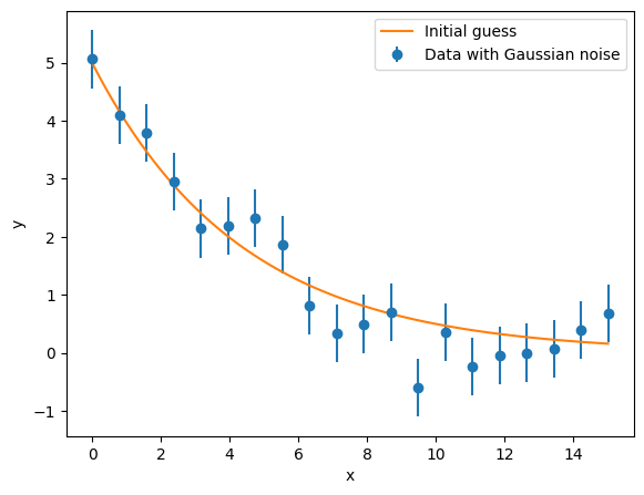
In order to fit to this data, create a Source where the experimental data is added.
datasource = satlas2.Source(data\_x, data\_y, yerr=yerr, name='ArtificialData')
This has generated a Source where both the x-values, y-values, and the uncertainty in y is known. As normal in SATLAS2, add the model to the Source and add the Source to a Fitter in order to start the fitting:
datasource.addModel(model)
f = satlas2.Fitter()
f.addSource(datasource)
The normal fitting can be done using the fit() method without any additional parameters.
f.fit()
print(f.reportFit())
\[\[Fit Statistics\]\]
\# fitting method = leastsq
\# function evals = 19
\# data points = 20
\# variables = 2
chi\-square \= 14.1856875
reduced chi\-square \= 0.78809375
Akaike info crit \= \-2.86997486
Bayesian info crit \= \-0.87851031
\[\[Variables\]\]
ArtificialData\_\_\_Exp\_\_\_amplitude: 5.25120089 +/- 0.33155088 (6.31%) (init \= 5)
ArtificialData\_\_\_Exp\_\_\_halflife: 2.70698749 +/- 0.26850056 (9.92%) (init \= 3)
Other fitting methods then _leastsq_ can be used by using the _method_ keyword.
f.revertFit() # To compare performance to normal fitting
f.fit(method='slsqp')
print(f.reportFit())
\[\[Fit Statistics\]\]
\# fitting method = SLSQP
\# function evals = 21
\# data points = 20
\# variables = 2
chi\-square \= 14.1856875
reduced chi\-square \= 0.78809375
Akaike info crit \= \-2.86997486
Bayesian info crit \= \-0.87851031
\[\[Variables\]\]
ArtificialData\_\_\_Exp\_\_\_amplitude: 5.25120090 +/- 0.32314795 (6.15%) (init \= 5)
ArtificialData\_\_\_Exp\_\_\_halflife: 2.70698589 +/- 0.25131419 (9.28%) (init \= 3)
The LMFIT library exposes the following fitting algorithms for use:
> * ‘leastsq’: Levenberg-Marquardt (default)
>
> * ‘least\_squares’: Least-Squares minimization, using Trust Region Reflective method
>
> * ‘differential\_evolution’: differential evolution
>
> * ‘brute’: brute force method
>
> * ‘basinhopping’: basinhopping
>
> * ‘ampgo’: Adaptive Memory Programming for Global Optimization
>
> * ‘nelder’: Nelder-Mead
>
> * ‘lbfgsb’: L-BFGS-B
>
> * ‘powell’: Powell
>
> * ‘cg’: Conjugate-Gradient
>
> * ‘newton’: Newton-CG
>
> * ‘cobyla’: Cobyla
>
> * ‘bfgs’: BFGS
>
> * ‘tnc’: Truncated Newton
>
> * ‘trust-ncg’: Newton-CG trust-region
>
> * ‘trust-exact’: nearly exact trust-region
>
> * ‘trust-krylov’: Newton GLTR trust-region
>
> * ‘trust-constr’: trust-region for constrained optimization
>
> * ‘dogleg’: Dog-leg trust-region
>
> * ‘slsqp’: Sequential Linear Squares Programming
>
> * ‘emcee’: Maximum likelihood via Monte-Carlo Markov Chain
>
> * ‘shgo’: Simplicial Homology Global Optimization
>
> * ‘dual\_annealing’: Dual Annealing optimization
>
However, some of these methods require the Jacobian or explicit boundaries for all parameters to be provided. Therefore, the following algorithms are recommended as options for SATLAS2:
> * ‘leastsq’: Levenberg-Marquardt (default)
>
> * ‘least\_squares’: Least-Squares minimization, using Trust Region Reflective method
>
> * ‘basinhopping’: basinhopping
>
> * ‘ampgo’: Adaptive Memory Programming for Global Optimization
>
> * ‘nelder’: Nelder-Mead
>
> * ‘lbfgsb’: L-BFGS-B
>
> * ‘powell’: Powell
>
> * ‘cg’: Conjugate-Gradient
>
> * ‘cobyla’: Cobyla
>
> * ‘bfgs’: BFGS
>
> * ‘tnc’: Truncated Newton
>
> * ‘trust-constr’: trust-region for constrained optimization
>
> * ‘slsqp’: Sequential Linear Squares Programming
>
> * ‘emcee’: Maximum likelihood via Monte-Carlo Markov Chain
>
As an example, the generated data is fitted with each of these algorithms, to show they give functionally the same answer. However, keep in mind that the speed and success of each algorithm depends on the data and model used, so not all algorithms may be suitable! As a rule of thumb, the least squares algorithms are among the most stable and widely applicable.
methods = \['leastsq',\
'least\_squares',\
'basinhopping',\
'ampgo',\
'nelder',\
'lbfgsb',\
'powell',\
'cg',\
'cobyla',\
'bfgs',\
'tnc',\
'trust-constr',\
'slsqp'\]
evals = \[\]
for m in methods:
f.revertFit()
f.fit(method=m)
evals.append(f.result.nfev)
print(f.reportFit())
\[\[Fit Statistics\]\]
\# fitting method = leastsq
\# function evals = 19
\# data points = 20
\# variables = 2
chi\-square \= 14.1856875
reduced chi\-square \= 0.78809375
Akaike info crit \= \-2.86997486
Bayesian info crit \= \-0.87851031
\[\[Variables\]\]
ArtificialData\_\_\_Exp\_\_\_amplitude: 5.25120089 +/- 0.33155088 (6.31%) (init \= 5)
ArtificialData\_\_\_Exp\_\_\_halflife: 2.70698749 +/- 0.26850056 (9.92%) (init \= 3)
\[\[Fit Statistics\]\]
\# fitting method = least\_squares
\# function evals = 7
\# data points = 20
\# variables = 2
chi\-square \= 14.1856875
reduced chi\-square \= 0.78809375
Akaike info crit \= \-2.86997486
Bayesian info crit \= \-0.87851031
\[\[Variables\]\]
ArtificialData\_\_\_Exp\_\_\_amplitude: 5.25120089 +/- 0.33154988 (6.31%) (init \= 5)
ArtificialData\_\_\_Exp\_\_\_halflife: 2.70698749 +/- 0.26850333 (9.92%) (init \= 3)
\[\[Fit Statistics\]\]
\# fitting method = basinhopping
\# function evals = 2505
\# data points = 20
\# variables = 2
chi\-square \= 14.1856875
reduced chi\-square \= 0.78809375
Akaike info crit \= \-2.86997486
Bayesian info crit \= \-0.87851031
\[\[Variables\]\]
ArtificialData\_\_\_Exp\_\_\_amplitude: 5.25120348 +/- 0.32314799 (6.15%) (init \= 5)
ArtificialData\_\_\_Exp\_\_\_halflife: 2.70698420 +/- 0.25131396 (9.28%) (init \= 3)
\[\[Fit Statistics\]\]
\# fitting method = ampgo, with L-BFGS-B as local solver
\# function evals = 4644
\# data points = 20
\# variables = 2
chi\-square \= 14.1856875
reduced chi\-square \= 0.78809375
Akaike info crit \= \-2.86997486
Bayesian info crit \= \-0.87851031
\[\[Variables\]\]
ArtificialData\_\_\_Exp\_\_\_amplitude: 5.25120344 +/- 0.32314799 (6.15%) (init \= 5)
ArtificialData\_\_\_Exp\_\_\_halflife: 2.70698421 +/- 0.25131396 (9.28%) (init \= 3)
\[\[Fit Statistics\]\]
\# fitting method = Nelder-Mead
\# function evals = 58
\# data points = 20
\# variables = 2
chi\-square \= 14.1856875
reduced chi\-square \= 0.78809375
Akaike info crit \= \-2.86997483
Bayesian info crit \= \-0.87851028
\[\[Variables\]\]
ArtificialData\_\_\_Exp\_\_\_amplitude: 5.25120285 +/- 0.32314600 (6.15%) (init \= 5)
ArtificialData\_\_\_Exp\_\_\_halflife: 2.70695228 +/- 0.25130868 (9.28%) (init \= 3)
\[\[Fit Statistics\]\]
\# fitting method = L-BFGS-B
\# function evals = 24
\# data points = 20
\# variables = 2
chi\-square \= 14.1856875
reduced chi\-square \= 0.78809375
Akaike info crit \= \-2.86997486
Bayesian info crit \= \-0.87851031
\[\[Variables\]\]
ArtificialData\_\_\_Exp\_\_\_amplitude: 5.25120344 +/- 0.32314799 (6.15%) (init \= 5)
ArtificialData\_\_\_Exp\_\_\_halflife: 2.70698421 +/- 0.25131396 (9.28%) (init \= 3)
\[\[Fit Statistics\]\]
\# fitting method = Powell
\# function evals = 70
\# data points = 20
\# variables = 2
chi\-square \= 14.1856882
reduced chi\-square \= 0.78809379
Akaike info crit \= \-2.86997382
Bayesian info crit \= \-0.87850927
\[\[Variables\]\]
ArtificialData\_\_\_Exp\_\_\_amplitude: 5.25117728 +/- 0.32313557 (6.15%) (init \= 5)
ArtificialData\_\_\_Exp\_\_\_halflife: 2.70680473 +/- 0.25128384 (9.28%) (init \= 3)
\[\[Fit Statistics\]\]
\# fitting method = CG
\# function evals = 33
\# data points = 20
\# variables = 2
chi\-square \= 14.1856875
reduced chi\-square \= 0.78809375
Akaike info crit \= \-2.86997486
Bayesian info crit \= \-0.87851031
\[\[Variables\]\]
ArtificialData\_\_\_Exp\_\_\_amplitude: 5.25120348 +/- 0.32314799 (6.15%) (init \= 5)
ArtificialData\_\_\_Exp\_\_\_halflife: 2.70698419 +/- 0.25131396 (9.28%) (init \= 3)
\[\[Fit Statistics\]\]
\# fitting method = COBYLA
\# function evals = 34
\# data points = 20
\# variables = 2
chi\-square \= 14.1856876
reduced chi\-square \= 0.78809375
Akaike info crit \= \-2.86997469
Bayesian info crit \= \-0.87851014
\[\[Variables\]\]
ArtificialData\_\_\_Exp\_\_\_amplitude: 5.25115052 +/- 0.32314226 (6.15%) (init \= 5)
ArtificialData\_\_\_Exp\_\_\_halflife: 2.70693798 +/- 0.25130535 (9.28%) (init \= 3)
\[\[Fit Statistics\]\]
\# fitting method = BFGS
\# function evals = 24
\# data points = 20
\# variables = 2
chi\-square \= 14.1856875
reduced chi\-square \= 0.78809375
Akaike info crit \= \-2.86997486
Bayesian info crit \= \-0.87851031
\[\[Variables\]\]
ArtificialData\_\_\_Exp\_\_\_amplitude: 5.25120352 +/- 0.32314799 (6.15%) (init \= 5)
ArtificialData\_\_\_Exp\_\_\_halflife: 2.70698416 +/- 0.25131395 (9.28%) (init \= 3)
\[\[Fit Statistics\]\]
\# fitting method = TNC
\# function evals = 156
\# data points = 20
\# variables = 2
chi\-square \= 14.1856875
reduced chi\-square \= 0.78809375
Akaike info crit \= \-2.86997485
Bayesian info crit \= \-0.87851031
\[\[Variables\]\]
ArtificialData\_\_\_Exp\_\_\_amplitude: 5.25117819 +/- 0.32314717 (6.15%) (init \= 5)
ArtificialData\_\_\_Exp\_\_\_halflife: 2.70699341 +/- 0.25131501 (9.28%) (init \= 3)
\[\[Fit Statistics\]\]
\# fitting method = equality\_constrained\_sqp
\# function evals = 69
\# data points = 20
\# variables = 2
chi\-square \= 14.1856875
reduced chi\-square \= 0.78809375
Akaike info crit \= \-2.86997486
Bayesian info crit \= \-0.87851031
\[\[Variables\]\]
ArtificialData\_\_\_Exp\_\_\_amplitude: 5.25120345 +/- 0.32314799 (6.15%) (init \= 5)
ArtificialData\_\_\_Exp\_\_\_halflife: 2.70698419 +/- 0.25131396 (9.28%) (init \= 3)
\[\[Fit Statistics\]\]
\# fitting method = SLSQP
\# function evals = 21
\# data points = 20
\# variables = 2
chi\-square \= 14.1856875
reduced chi\-square \= 0.78809375
Akaike info crit \= \-2.86997486
Bayesian info crit \= \-0.87851031
\[\[Variables\]\]
ArtificialData\_\_\_Exp\_\_\_amplitude: 5.25120090 +/- 0.32314795 (6.15%) (init \= 5)
ArtificialData\_\_\_Exp\_\_\_halflife: 2.70698589 +/- 0.25131419 (9.28%) (init \= 3)
indices = np.argsort(evals)
m = np.array(methods)
e = np.array(evals)
m = m\[indices\]
e = e\[indices\]
fig = plt.figure()
ax = fig.add\_axes(\[0.1, 0.1, 0.8, 0.8\])
ax.bar(m, e)
ax.set\_yscale('log')
xticklabels = ax.get\_xticklabels()
ax.set\_xticklabels(xticklabels, rotation = 45, ha="right")
ax.set\_ylabel('Function evaluations')
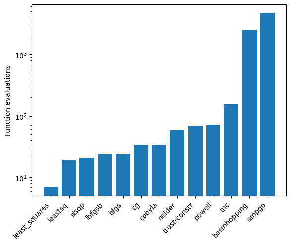
From experimenting with simulated and actual hyperfine laser spectroscopic data, the `slsqp` algorithm was found to offer both a relatively fast and stable platform.
Adding prior to parameters[#](https://iks-nm.github.io/satlas2/tutorials/fitting/index.html#adding-prior-to-parameters "Permalink to this heading")
----------------------------------------------------------------------------------------------------------------------------------------------------
Suppose a literature value is known and has to be applied to a parameter as an additional constraint. This can be viewed as a prior, or alternatively as an additional data point to fit to. A Gaussian prior can easily be added via the `setParamPrior` method of the Fitter object.
f.revertFit()
f.fit()
print(f.reportFit()) # Fit without prior
f.revertFit()
f.setParamPrior('ArtificialData', 'Exp', 'halflife', 3, 0.1) # Add prior to fit the halflife of model Exp in the source ArtificialData to 3+/-0.1
f.fit()
print(f.reportFit())
f.revertFit()
f.setParamPrior('ArtificialData', 'Exp', 'halflife', 3, 0.5) # Change the prior 3+/-0.5
f.fit()
print(f.reportFit())
f.revertFit()
f.removeParamPrior('ArtificialData', 'Exp', 'halflife') # Remove the prior
f.fit()
print(f.reportFit())
\[\[Fit Statistics\]\]
\# fitting method = leastsq
\# function evals = 19
\# data points = 20
\# variables = 2
chi\-square \= 14.1856875
reduced chi\-square \= 0.78809375
Akaike info crit \= \-2.86997486
Bayesian info crit \= \-0.87851031
\[\[Variables\]\]
ArtificialData\_\_\_Exp\_\_\_amplitude: 5.25120089 +/- 0.33155088 (6.31%) (init \= 5)
ArtificialData\_\_\_Exp\_\_\_halflife: 2.70698749 +/- 0.26850056 (9.92%) (init \= 3)
\[\[Fit Statistics\]\]
\# fitting method = leastsq
\# function evals = 10
\# data points = 21
\# variables = 2
chi\-square \= 15.0536495
reduced chi\-square \= 0.79229734
Akaike info crit \= \-2.99094168
Bayesian info crit \= \-0.90189680
\[\[Variables\]\]
ArtificialData\_\_\_Exp\_\_\_amplitude: 5.04903680 +/- 0.25418730 (5.03%) (init \= 5)
ArtificialData\_\_\_Exp\_\_\_halflife: 2.97175885 +/- 0.08528185 (2.87%) (init \= 3)
\[\[Fit Statistics\]\]
\# fitting method = leastsq
\# function evals = 16
\# data points = 21
\# variables = 2
chi\-square \= 14.4439027
reduced chi\-square \= 0.76020540
Akaike info crit \= \-3.85925151
Bayesian info crit \= \-1.77020663
\[\[Variables\]\]
ArtificialData\_\_\_Exp\_\_\_amplitude: 5.19393631 +/- 0.30407003 (5.85%) (init \= 5)
ArtificialData\_\_\_Exp\_\_\_halflife: 2.78050485 +/- 0.23033480 (8.28%) (init \= 3)
\[\[Fit Statistics\]\]
\# fitting method = leastsq
\# function evals = 19
\# data points = 20
\# variables = 2
chi\-square \= 14.1856875
reduced chi\-square \= 0.78809375
Akaike info crit \= \-2.86997486
Bayesian info crit \= \-0.87851031
\[\[Variables\]\]
ArtificialData\_\_\_Exp\_\_\_amplitude: 5.25120089 +/- 0.33155088 (6.31%) (init \= 5)
ArtificialData\_\_\_Exp\_\_\_halflife: 2.70698749 +/- 0.26850056 (9.92%) (init \= 3)
Fitting with likelihood data[#](https://iks-nm.github.io/satlas2/tutorials/fitting/index.html#fitting-with-likelihood-data "Permalink to this heading")
--------------------------------------------------------------------------------------------------------------------------------------------------------
The fitting can also proceed by maximizing the likelihood (or rather, minimizing the negative loglikelihood) instead of minimizing the chisquare. In order to do this, use the _llh=True_ parameter in the fitting routine.
Currently, there are two options for the likelihood, which can be set with the _llh\_method_ keyword: _gaussian_ (the default) and _poisson_. When the likelihood fitting is used, the _leastsq_ and _least\_squares_ methods cannot be applied since the negative loglikelihood is no longer a sum of squares, an assumption which is critical in these algorithms.
f.revertFit()
f.fit(llh=True)
print(f.reportFit())
f.revertFit()
f.setParamPrior('ArtificialData', 'Exp', 'halflife', 3, 0.1) # Prior of 3+/-0.1
f.fit(llh=True)
print(f.reportFit())
\[\[Fit Statistics\]\]
\# fitting method = SLSQP
\# function evals = 20
\# data points = 20
\# variables = 2
chi\-square \= 8.21548506
reduced chi\-square \= 0.45641584
Akaike info crit \= \-13.7942296
Bayesian info crit \= \-11.8027650
\[\[Variables\]\]
ArtificialData\_\_\_Exp\_\_\_amplitude: 5.25117472 +/- 0.51478516 (9.80%) (init \= 5)
ArtificialData\_\_\_Exp\_\_\_halflife: 2.70699167 +/- 0.40035373 (14.79%) (init \= 3)
\[\[Fit Statistics\]\]
\# fitting method = SLSQP
\# function evals = 15
\# data points = 21
\# variables = 2
chi\-square \= 9.84186102
reduced chi\-square \= 0.51799269
Akaike info crit \= \-11.9154300
Bayesian info crit \= \-9.82638508
\[\[Variables\]\]
ArtificialData\_\_\_Exp\_\_\_amplitude: 5.04906321 +/- 0.40525527 (8.03%) (init \= 5)
ArtificialData\_\_\_Exp\_\_\_halflife: 2.97176292 +/- 0.13544977 (4.56%) (init \= 3)
Notice that the reduced chisquare is still reported. However, in this mode, it _no longer_ is a valid statistical measure to look at! This is also the reason why the uncertainties are different. The estimation of the uncertainties is done by numerically approximating the Hessian matrix of the problem and inverting it, and this is also done in the chisquare methods. The reason it now differs is twofold: - The matrix describing the problem is different, hence some numerical approximations can give slightlly different results. - Since the reduced chisquare is no longer a valid statistical measure, it can no longer be used to scale the uncertainties!
Using Poisson likelihood[#](https://iks-nm.github.io/satlas2/tutorials/fitting/index.html#using-poisson-likelihood "Permalink to this heading")
------------------------------------------------------------------------------------------------------------------------------------------------
Up to here, the likelihood fitting was focused on Gaussian uncertainties, but a Poisson statistic can also be used for the likelihood calculation. This option will be illustrated on artificial hyperfine data.
spin = 3.5
J = \[0.5, 1.5\]
A = \[9600, 175\]
B = \[0, 315\]
C = \[0, 0\]
FWHMG = 135
FWHML = 101
centroid = 480
bkg = 1
scale = 90
x = np.arange(-17500, -14500, 40)
x = np.hstack(\[x, np.arange(20000, 23000, 40)\])
rng = np.random.default\_rng(0)
f = satlas2.Fitter()
hfs = satlas2.HFS(spin,
J,
A=A,
B=B,
C=C,
scale=scale,
df=centroid,
name='HFS1',
racah=True,
fwhmg=FWHMG,
fwhml=FWHML)
bkgm = satlas2.Polynomial(\[bkg\], name='bkg1')
y = satlas2.generateSpectrum(\[hfs, bkgm\], x, rng.poisson)
datasource = satlas2.Source(x,
y,
yerr=modifiedSqrt,
name='Scan1')
datasource.addModel(hfs)
datasource.addModel(bkgm)
f.addSource(datasource)
def plot\_hfs(f):
fig = plt.figure(constrained\_layout=True)
gs = gridspec.GridSpec(nrows=len(f.sources), ncols=2, figure=fig)
a1 = None
a2 = None
axes = \[\]
for i, (name, datasource) in enumerate(f.sources):
if a1 is None:
ax1 = fig.add\_subplot(gs\[i, 0\])
ax2 = fig.add\_subplot(gs\[i, 1\])
a1 = ax1
a2 = ax2
else:
ax1 = fig.add\_subplot(gs\[i, 0\], sharex=a1)
ax2 = fig.add\_subplot(gs\[i, 1\], sharex=a2)
left = datasource.x < 0
right = datasource.x > 0
smooth\_left = np.arange(datasource.x\[left\].min(), datasource.x\[left\].max(),
5.0)
smooth\_right = np.arange(datasource.x\[right\].min(),
datasource.x\[right\].max(), 5.0)
ax1.plot(datasource.x\[left\],
datasource.y\[left\],
drawstyle='steps-mid',
label='Data')
ax1.plot(smooth\_left, datasource.evaluate(smooth\_left), label='Fit')
ax2.plot(datasource.x\[right\],
datasource.y\[right\],
drawstyle='steps-mid',
label='Data')
ax2.plot(smooth\_right, datasource.evaluate(smooth\_right), label='Fit')
ax1.set\_xlabel('Frequency \[MHz\]')
ax2.set\_xlabel('Frequency \[MHz\]')
ax1.set\_ylabel('Counts')
ax2.set\_ylabel('Counts')
ax1.label\_outer()
ax2.label\_outer()
axes.append(\[ax1, ax2\])
plot\_hfs(f)
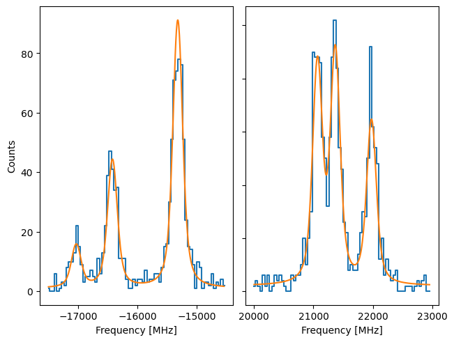
Notice that here, the _yerr_ supplied to the Source is not an array, but instead a function. When this is the case, the uncertainty on y is calculated by applying the function to the sum of the underlying models. In this case, this would give rise to using Pearson’s chisquare, where the uncertainty on the datapoint is given by sqrt(f(x)). A preliminary fit can be done by using the normal chisquare fitting.
f.fit()
plot\_hfs(f)
print(f.reportFit())
\[\[Fit Statistics\]\]
\# fitting method = leastsq
\# function evals = 61
\# data points = 150
\# variables = 9
chi\-square \= 145.269585
reduced chi\-square \= 1.03028075
Akaike info crit \= 13.1933897
Bayesian info crit \= 40.2891074
\[\[Variables\]\]
Scan1\_\_\_HFS1\_\_\_centroid: 479.080650 +/- 3.21744678 (0.67%) (init \= 480)
Scan1\_\_\_HFS1\_\_\_Al: 9602.87663 +/- 2.38671593 (0.02%) (init \= 9600)
Scan1\_\_\_HFS1\_\_\_Au: 176.326690 +/- 1.06392599 (0.60%) (init \= 175)
Scan1\_\_\_HFS1\_\_\_Bl: 0 (fixed)
Scan1\_\_\_HFS1\_\_\_Bu: 320.837280 +/- 8.31153123 (2.59%) (init \= 315)
Scan1\_\_\_HFS1\_\_\_Cl: 0 (fixed)
Scan1\_\_\_HFS1\_\_\_Cu: 0.28989447 +/- 0.64808883 (223.56%) (init \= 0)
Scan1\_\_\_HFS1\_\_\_FWHMG: 124.983331 +/- 20.4156372 (16.33%) (init \= 135)
Scan1\_\_\_HFS1\_\_\_FWHML: 115.427701 +/- 16.2067792 (14.04%) (init \= 101)
Scan1\_\_\_HFS1\_\_\_scale: 93.1256964 +/- 4.04213464 (4.34%) (init \= 90)
Scan1\_\_\_HFS1\_\_\_Amp3to2: 0.4545455 (fixed)
Scan1\_\_\_HFS1\_\_\_Amp3to3: 0.4772727 (fixed)
Scan1\_\_\_HFS1\_\_\_Amp3to4: 0.3409091 (fixed)
Scan1\_\_\_HFS1\_\_\_Amp4to3: 0.1590909 (fixed)
Scan1\_\_\_HFS1\_\_\_Amp4to4: 0.4772727 (fixed)
Scan1\_\_\_HFS1\_\_\_Amp4to5: 1 (fixed)
Scan1\_\_\_bkg1\_\_\_p0: 1.32051846 +/- 0.29450939 (22.30%) (init \= 1)
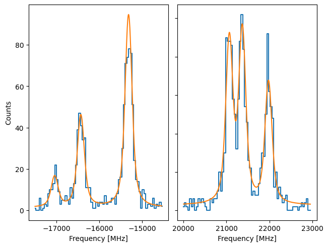
We can see the difference by comparing to a Source where the uncertainty in y is given by the square root:
yerr = modifiedSqrt(y)
f2 = satlas2.Fitter()
hfs2 = satlas2.HFS(spin,
J,
A=A,
B=B,
C=C,
scale=scale,
df=centroid,
name='HFS1',
racah=True,
fwhmg=FWHMG,
fwhml=FWHML)
bkgm2 = satlas2.Polynomial(\[bkg\], name='bkg1')
datasource2 = satlas2.Source(x,
y,
yerr=yerr,
name='Scan1')
datasource2.addModel(hfs2)
datasource2.addModel(bkgm2)
f2.addSource(datasource2)
f2.fit()
plot\_hfs(f2)
print(f2.reportFit())
\[\[Fit Statistics\]\]
\# fitting method = leastsq
\# function evals = 51
\# data points = 150
\# variables = 9
chi\-square \= 154.121394
reduced chi\-square \= 1.09305953
Akaike info crit \= 22.0657907
Bayesian info crit \= 49.1615083
\[\[Variables\]\]
Scan1\_\_\_HFS1\_\_\_centroid: 478.154622 +/- 3.14574940 (0.66%) (init \= 480)
Scan1\_\_\_HFS1\_\_\_Al: 9603.17923 +/- 2.31958026 (0.02%) (init \= 9600)
Scan1\_\_\_HFS1\_\_\_Au: 175.647786 +/- 1.02797017 (0.59%) (init \= 175)
Scan1\_\_\_HFS1\_\_\_Bl: 0 (fixed)
Scan1\_\_\_HFS1\_\_\_Bu: 324.809731 +/- 8.15038145 (2.51%) (init \= 315)
Scan1\_\_\_HFS1\_\_\_Cl: 0 (fixed)
Scan1\_\_\_HFS1\_\_\_Cu: 0.53845378 +/- 0.60603957 (112.55%) (init \= 0)
Scan1\_\_\_HFS1\_\_\_FWHMG: 155.650412 +/- 15.1637090 (9.74%) (init \= 135)
Scan1\_\_\_HFS1\_\_\_FWHML: 81.1159460 +/- 13.7997436 (17.01%) (init \= 101)
Scan1\_\_\_HFS1\_\_\_scale: 91.2170258 +/- 3.69217051 (4.05%) (init \= 90)
Scan1\_\_\_HFS1\_\_\_Amp3to2: 0.4545455 (fixed)
Scan1\_\_\_HFS1\_\_\_Amp3to3: 0.4772727 (fixed)
Scan1\_\_\_HFS1\_\_\_Amp3to4: 0.3409091 (fixed)
Scan1\_\_\_HFS1\_\_\_Amp4to3: 0.1590909 (fixed)
Scan1\_\_\_HFS1\_\_\_Amp4to4: 0.4772727 (fixed)
Scan1\_\_\_HFS1\_\_\_Amp4to5: 1 (fixed)
Scan1\_\_\_bkg1\_\_\_p0: 0.54384301 +/- 0.22795427 (41.92%) (init \= 1)
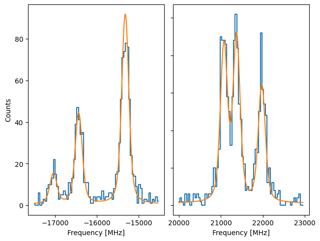
While not extremely large, there is a noticable difference between the results. The Pearson’s chisquare is recommended since this is the better approximation of the Poisson statistics.
However, the Poisson likellihood can also be used to fit the spectrum:
f.revertFit()
f.fit(llh=True, llh\_method='poisson')
print(f.reportFit())
plot\_hfs(f)
\[\[Fit Statistics\]\]
\# fitting method = SLSQP
\# function evals = 352
\# data points = 150
\# variables = 9
chi\-square \= 527353.038
reduced chi\-square \= 3740.09247
Akaike info crit \= 1242.74853
Bayesian info crit \= 1269.84425
\[\[Variables\]\]
Scan1\_\_\_HFS1\_\_\_centroid: 479.100586 +/- 4.33513046 (0.90%) (init \= 480)
Scan1\_\_\_HFS1\_\_\_Al: 9602.92888 +/- 3.15529346 (0.03%) (init \= 9600)
Scan1\_\_\_HFS1\_\_\_Au: 176.139805 +/- 1.41592721 (0.80%) (init \= 175)
Scan1\_\_\_HFS1\_\_\_Bl: 0 (fixed)
Scan1\_\_\_HFS1\_\_\_Bu: 322.344602 +/- 11.1539978 (3.46%) (init \= 315)
Scan1\_\_\_HFS1\_\_\_Cl: 0 (fixed)
Scan1\_\_\_HFS1\_\_\_Cu: 0.34831527 +/- 0.85318133 (244.95%) (init \= 0)
Scan1\_\_\_HFS1\_\_\_FWHMG: 126.466451 +/- 24.1675668 (19.11%) (init \= 135)
Scan1\_\_\_HFS1\_\_\_FWHML: 114.489689 +/- 19.6138914 (17.13%) (init \= 101)
Scan1\_\_\_HFS1\_\_\_scale: 93.0371162 +/- 5.32580850 (5.72%) (init \= 90)
Scan1\_\_\_HFS1\_\_\_Amp3to2: 0.4545455 (fixed)
Scan1\_\_\_HFS1\_\_\_Amp3to3: 0.4772727 (fixed)
Scan1\_\_\_HFS1\_\_\_Amp3to4: 0.3409091 (fixed)
Scan1\_\_\_HFS1\_\_\_Amp4to3: 0.1590909 (fixed)
Scan1\_\_\_HFS1\_\_\_Amp4to4: 0.4772727 (fixed)
Scan1\_\_\_HFS1\_\_\_Amp4to5: 1 (fixed)
Scan1\_\_\_bkg1\_\_\_p0: 0.83471487 +/- 0.33553551 (40.20%) (init \= 1)
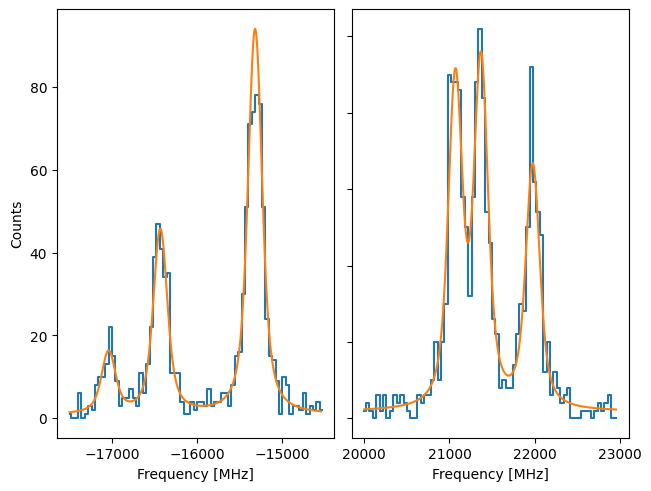
Here, it’s more than clear that the (reduced) chisquare is not usable, since LMFIT internally _assumes_ what is returned in the cost function is the chisquare statistic.
Using `emcee`[#](https://iks-nm.github.io/satlas2/tutorials/fitting/index.html#using-emcee "Permalink to this heading")
------------------------------------------------------------------------------------------------------------------------
One option that is given by LMFIT as an optimizer but not demonstrated is the `emcee` option. Using this, the returned value is treated as a loglikelihood for a random walk algorithm. By using many walkers to sample the loglikelihood, a very good approximation of the probability density function is generated. For more information, see the documentation of the `emcee` package.
Here, the basic usage in SATLAS2 will be illustrated, along with some advanced topic to modify the working of the underlying algorithm.
f.revertFit()
f.fit(llh=True, llh\_method='poisson', method='emcee', steps=1000, nwalkers=50)
print(f.reportFit())
100%|█████████████████████████████████████████████████████| 1000/1000 \[00:10<00:00, 91.95it/s\]
The chain is shorter than 50 times the integrated autocorrelation time for 8 parameter(s). Use this estimate with caution and run a longer chain!
N/50 = 20;
tau: \[56.03746971 50.19572236 48.76119684 54.62125998 nan 55.75800502\
57.46850239 48.427324 51.04319725\]
\[\[Fit Statistics\]\]
# fitting method = emcee
# function evals = 50000
# data points = 1
# variables = 9
chi-square = 0.00000000
reduced chi-square = 0.00000000
Akaike info crit = -8148.27696
Bayesian info crit = -8166.27696
\[\[Variables\]\]
Scan1\_\_\_HFS1\_\_\_centroid: 478.754968 +/- 3.36112524 (0.70%) (init = 480)
Scan1\_\_\_HFS1\_\_\_Al: 9602.88489 +/- 2.47289183 (0.03%) (init = 9600)
Scan1\_\_\_HFS1\_\_\_Au: 176.147526 +/- 1.09427588 (0.62%) (init = 175)
Scan1\_\_\_HFS1\_\_\_Bl: 0 (fixed)
Scan1\_\_\_HFS1\_\_\_Bu: 322.133034 +/- 8.61135651 (2.67%) (init = 315)
Scan1\_\_\_HFS1\_\_\_Cl: 0 (fixed)
Scan1\_\_\_HFS1\_\_\_Cu: 0.00000000 +/- 0.00000000 (nan%) (init = 0)
Scan1\_\_\_HFS1\_\_\_FWHMG: 127.070329 +/- 18.2713574 (14.38%) (init = 135)
Scan1\_\_\_HFS1\_\_\_FWHML: 114.104097 +/- 15.0276800 (13.17%) (init = 101)
Scan1\_\_\_HFS1\_\_\_scale: 92.2315758 +/- 3.90345595 (4.23%) (init = 90)
Scan1\_\_\_HFS1\_\_\_Amp3to2: 0.4545455 (fixed)
Scan1\_\_\_HFS1\_\_\_Amp3to3: 0.4772727 (fixed)
Scan1\_\_\_HFS1\_\_\_Amp3to4: 0.3409091 (fixed)
Scan1\_\_\_HFS1\_\_\_Amp4to3: 0.1590909 (fixed)
Scan1\_\_\_HFS1\_\_\_Amp4to4: 0.4772727 (fixed)
Scan1\_\_\_HFS1\_\_\_Amp4to5: 1 (fixed)
Scan1\_\_\_bkg1\_\_\_p0: 0.88489588 +/- 0.24745153 (27.96%) (init = 1)
The results of the fitting are calculated by taking the median of the samples as the central value, and the average of the one-sided 1-sigma as the general uncertainty on the parameter. However, fitting this way loses some information, since there is no saved record of the sampled parameters, and the validity of the walk cannot be tested. In particular, note that Cu has a peculiar value which requires some investigation.
In order to do this, the chain of samples can be saved by specifying a filename:
f.revertFit()
filename = 'emceeDemonstration.h5'
f.fit(llh=True, llh\_method='poisson', method='emcee', steps=1000, nwalkers=50, filename=filename)
print(f.reportFit())
100%|█████████████████████████████████████████████████████| 1000/1000 \[00:18<00:00, 53.99it/s\]
The chain is shorter than 50 times the integrated autocorrelation time for 8 parameter(s). Use this estimate with caution and run a longer chain!
N/50 = 20;
tau: \[57.04341752 53.56998762 54.11377706 55.15716973 nan 53.95575965\
60.18713051 50.04226876 55.48363343\]
\[\[Fit Statistics\]\]
# fitting method = emcee
# function evals = 50000
# data points = 1
# variables = 9
chi-square = 0.00000000
reduced chi-square = 0.00000000
Akaike info crit = -8148.29278
Bayesian info crit = -8166.29278
\[\[Variables\]\]
Scan1\_\_\_HFS1\_\_\_centroid: 479.119418 +/- 3.23737942 (0.68%) (init = 480)
Scan1\_\_\_HFS1\_\_\_Al: 9602.76065 +/- 2.51181010 (0.03%) (init = 9600)
Scan1\_\_\_HFS1\_\_\_Au: 176.127101 +/- 1.10213818 (0.63%) (init = 175)
Scan1\_\_\_HFS1\_\_\_Bl: 0 (fixed)
Scan1\_\_\_HFS1\_\_\_Bu: 320.765821 +/- 8.85014810 (2.76%) (init = 315)
Scan1\_\_\_HFS1\_\_\_Cl: 0 (fixed)
Scan1\_\_\_HFS1\_\_\_Cu: 0.00000000 +/- 0.00000000 (nan%) (init = 0)
Scan1\_\_\_HFS1\_\_\_FWHMG: 129.179634 +/- 18.3504559 (14.21%) (init = 135)
Scan1\_\_\_HFS1\_\_\_FWHML: 112.856566 +/- 15.0718209 (13.35%) (init = 101)
Scan1\_\_\_HFS1\_\_\_scale: 92.4039066 +/- 4.05517245 (4.39%) (init = 90)
Scan1\_\_\_HFS1\_\_\_Amp3to2: 0.4545455 (fixed)
Scan1\_\_\_HFS1\_\_\_Amp3to3: 0.4772727 (fixed)
Scan1\_\_\_HFS1\_\_\_Amp3to4: 0.3409091 (fixed)
Scan1\_\_\_HFS1\_\_\_Amp4to3: 0.1590909 (fixed)
Scan1\_\_\_HFS1\_\_\_Amp4to4: 0.4772727 (fixed)
Scan1\_\_\_HFS1\_\_\_Amp4to5: 1 (fixed)
Scan1\_\_\_bkg1\_\_\_p0: 0.86826205 +/- 0.23783254 (27.39%) (init = 1)
The fit resulted in the same parametervalues, so the saved chain can be used to analyse why Cu is causing issues. In order to do this, one of the ways to visualise the result is by looking at the plot of the walkers:
satlas2.generateWalkPlot(filename)
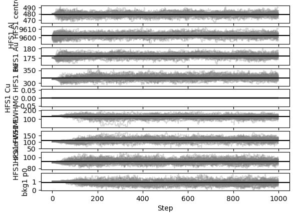
As the walkers progress towards their 1000 steps, nearly all parameters leave their phase of only exploring a tiny bit around the initial value and properly spread out. This burn-in phase is generally regarded as an undesired feature of the random walk algorithm and is normally discarded. Based on this plot, a claim for a burn-in phase of about 200 steps can be made.
In order to see the results for Cu in more detail, the results can be filtered:
satlas2.generateWalkPlot(filename, filter=\['Cu'\])
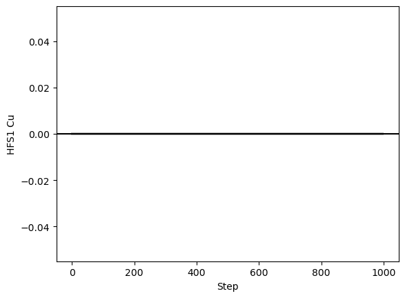
As can be seen here, there is absolutely no variation in the Cu value. One of the possibilities that spring to mind is that the boundaries put on the parameter force it to be 0. If that were the case however, the fitting with other routines would also have restricted the value to 0, which it hasn’t. Another assumption is that the value of _exactly_ 0 can be an issue for the random walker. This can be tested by reverting the fit, slightly adjusting the value (either directly or by doing a preliminary fit), and performing the random walk again.
f.revertFit()
f.fit()
filename = 'emceeDemonstrationCu.h5'
f.fit(llh=True, llh\_method='poisson', method='emcee', steps=1000, nwalkers=50, filename=filename)
satlas2.generateWalkPlot(filename, filter=\['Cu', 'Al', 'Au'\])
print(f.reportFit())
100%|█████████████████████████████████████████████████████| 1000/1000 \[00:18<00:00, 53.63it/s\]
The chain is shorter than 50 times the integrated autocorrelation time for 9 parameter(s). Use this estimate with caution and run a longer chain!
N/50 = 20;
tau: \[49.79535749 56.83821005 52.78761371 54.3836919 49.65206895 47.99592459\
50.88289254 49.70732336 74.38901137\]
\[\[Fit Statistics\]\]
\# fitting method = emcee
\# function evals = 50000
\# data points = 1
\# variables = 9
chi\-square \= 0.00000000
reduced chi\-square \= 0.00000000
Akaike info crit \= \-8148.56089
Bayesian info crit \= \-8166.56089
\[\[Variables\]\]
Scan1\_\_\_HFS1\_\_\_centroid: 479.179130 +/- 3.15197251 (0.66%) (init \= 479.0807)
Scan1\_\_\_HFS1\_\_\_Al: 9603.03121 +/- 2.31025284 (0.02%) (init \= 9602.877)
Scan1\_\_\_HFS1\_\_\_Au: 176.165779 +/- 1.01302344 (0.58%) (init \= 176.3267)
Scan1\_\_\_HFS1\_\_\_Bl: 0 (fixed)
Scan1\_\_\_HFS1\_\_\_Bu: 322.223737 +/- 7.69174619 (2.39%) (init \= 320.8373)
Scan1\_\_\_HFS1\_\_\_Cl: 0 (fixed)
Scan1\_\_\_HFS1\_\_\_Cu: 0.29007848 +/- 0.48222380 (166.24%) (init \= 0.2898991)
Scan1\_\_\_HFS1\_\_\_FWHMG: 126.034020 +/- 16.4263323 (13.03%) (init \= 124.9833)
Scan1\_\_\_HFS1\_\_\_FWHML: 114.134035 +/- 13.4331215 (11.77%) (init \= 115.4277)
Scan1\_\_\_HFS1\_\_\_scale: 92.8760544 +/- 3.69820672 (3.98%) (init \= 93.1257)
Scan1\_\_\_HFS1\_\_\_Amp3to2: 0.4545455 (fixed)
Scan1\_\_\_HFS1\_\_\_Amp3to3: 0.4772727 (fixed)
Scan1\_\_\_HFS1\_\_\_Amp3to4: 0.3409091 (fixed)
Scan1\_\_\_HFS1\_\_\_Amp4to3: 0.1590909 (fixed)
Scan1\_\_\_HFS1\_\_\_Amp4to4: 0.4772727 (fixed)
Scan1\_\_\_HFS1\_\_\_Amp4to5: 1 (fixed)
Scan1\_\_\_bkg1\_\_\_p0: 0.90596271 +/- 0.28898660 (31.90%) (init \= 1.320519)
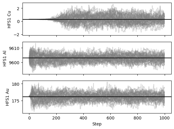
This shows that indeed, the value of exactly 0 is an issue for the random walker!
However, the small value of Cu in general lead to a much larger burn-in time, now more along the lines of 300-400 steps. By utilizing a burn-in time of 400 steps, more than enough samples are still present to generate a corner plot, where the 1D and 2D distributions of the samples is presented.
satlas2.generateCorrelationPlot(filename, burnin=400)
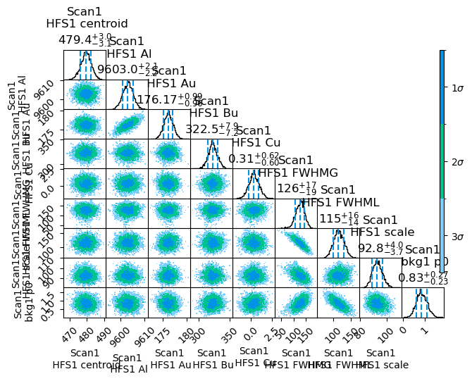
For clarity, this plot can also be filtered to only the parameters that are of interest. For further modification, the binning can be reduced with keywords:
satlas2.generateCorrelationPlot(filename, filter=\['Al', 'Au', 'Cu'\], burnin=400, binreduction=2, bin2dreduction=2)
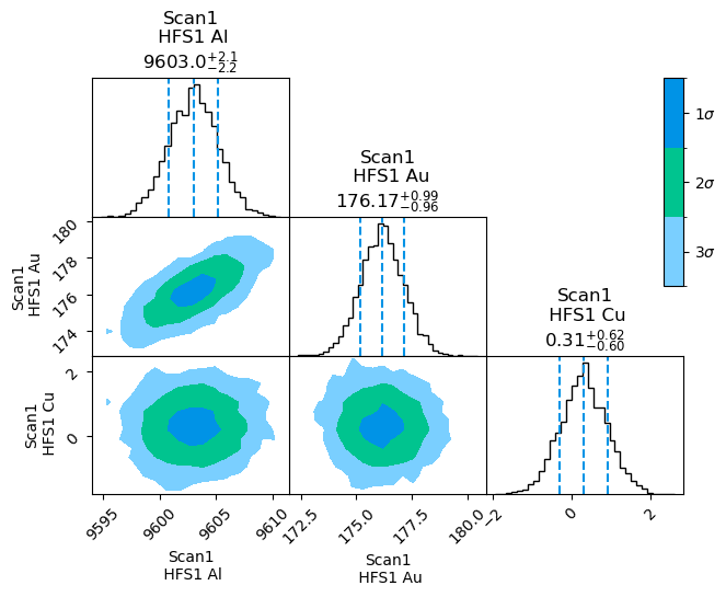
Now only the hyperfine parameters are shown. The number of bins in the 1D case has been reduced by a factor 2, and the number of bins in the 2D case by a further factor of 2, for a total reduction of 4 compared to the previous plot.
Overall, the results here are shown to be quite Gaussian, and can be used in the normal way. One more adaptation that can be made is removing the burn-in from the results. This can be done by processing the random walk with the _readWalk_ method of the Fitter.
f.readWalk(filename, burnin=400)
print(f.reportFit())
The chain is shorter than 50 times the integrated autocorrelation time for 9 parameter(s). Use this estimate with caution and run a longer chain!
N/50 = 12;
tau: \[45.62991851 40.32541678 37.45399196 39.03747261 40.87049522 37.94803522\
40.69432958 39.98245743 37.78922749\]
\[\[Fit Statistics\]\]
# fitting method = emcee
# function evals = 30000
# data points = unknown
# variables = 9
chi-square = unknown
reduced chi-square = unknown
Akaike info crit = unknown
Bayesian info crit = unknown
\[\[Variables\]\]
Scan1\_\_\_HFS1\_\_\_centroid: 479.423946 +/- 3.02033029 (0.63%) (init = 479.1791)
Scan1\_\_\_HFS1\_\_\_Al: 9603.01272 +/- 2.17492439 (0.02%) (init = 9603.031)
Scan1\_\_\_HFS1\_\_\_Au: 176.168601 +/- 0.97595651 (0.55%) (init = 176.1658)
Scan1\_\_\_HFS1\_\_\_Bl: 0 (fixed)
Scan1\_\_\_HFS1\_\_\_Bu: 322.518878 +/- 7.52505337 (2.33%) (init = 322.2237)
Scan1\_\_\_HFS1\_\_\_Cl: 0 (fixed)
Scan1\_\_\_HFS1\_\_\_Cu: 0.30503616 +/- 0.60819137 (199.38%) (init = 0.2900785)
Scan1\_\_\_HFS1\_\_\_FWHMG: 126.223702 +/- 17.9552979 (14.22%) (init = 126.034)
Scan1\_\_\_HFS1\_\_\_FWHML: 114.555690 +/- 14.8834032 (12.99%) (init = 114.134)
Scan1\_\_\_HFS1\_\_\_scale: 92.8395450 +/- 3.89293442 (4.19%) (init = 92.87605)
Scan1\_\_\_HFS1\_\_\_Amp3to2: 0.4545455 (fixed)
Scan1\_\_\_HFS1\_\_\_Amp3to3: 0.4772727 (fixed)
Scan1\_\_\_HFS1\_\_\_Amp3to4: 0.3409091 (fixed)
Scan1\_\_\_HFS1\_\_\_Amp4to3: 0.1590909 (fixed)
Scan1\_\_\_HFS1\_\_\_Amp4to4: 0.4772727 (fixed)
Scan1\_\_\_HFS1\_\_\_Amp4to5: 1 (fixed)
Scan1\_\_\_bkg1\_\_\_p0: 0.83493074 +/- 0.24998430 (29.94%) (init = 0.9059627)
The burnin has been processed correctly, as the value of e.g. Cu has been modified from 0.29+/-0.48 to 0.3+/-0.6, which is what the processed plot shows it should be.
Contents
---
# Unknown
Tutorial ======== .. toctree:: createmodel/index fitting/index dataframe/index walkoptions/index benchmark/index interface/index
---
# Making a model — SATLAS2
[Skip to main content](https://iks-nm.github.io/satlas2/tutorials/createmodel/index.html#main-content)
Back to top Ctrl+K
[ \
\
SATLAS2](https://iks-nm.github.io/satlas2/index.html)
Search Ctrl+K
* [Repository](https://github.com/iks-nm/satlas2)
* [Suggest edit](https://github.com/iks-nm/satlas2/edit/master/tutorials/createmodel/index.rst)
* [Open issue](https://github.com/iks-nm/satlas2/issues/new?title=Issue%20on%20page%20%2Ftutorials/createmodel/index.html&body=Your%20issue%20content%20here.)
* [.rst](https://iks-nm.github.io/satlas2/_sources/tutorials/createmodel/index.rst)
* .pdf
Light Dark System Settings
Making a model
==============
Contents
--------
Making a model[#](https://iks-nm.github.io/satlas2/tutorials/createmodel/index.html#making-a-model "Permalink to this heading")
================================================================================================================================
As illustrated in the architecture page, SATLAS2 is built on the concept of a Fitter object, to which Source objects are assigned. These Source objects contain both experimental data, but are also assigned one or more Models, which should be fitted to the data.
The base aspect of these Models is that two things should be implemented: a _params_ attribute which is a dictionary containing all the Parameters that the Model needs, and a method _f(x)_, where the response for the given _x_ values is returned. It is recommended that the first line of the method is _x = self.transform(x)_ in order to correctly handle any transformation functions that are required.
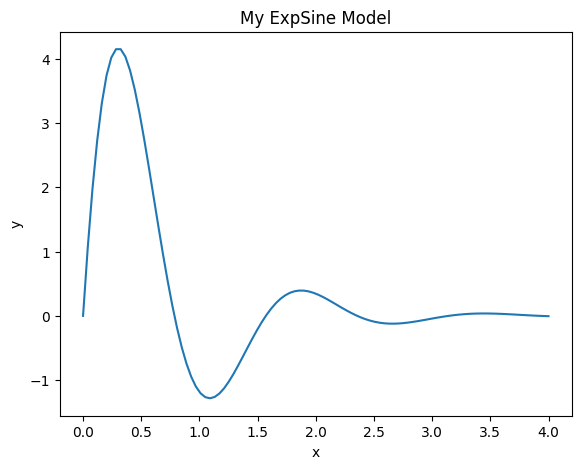
In this tutorial, a new Model will be created to model a sine wave with exponential damping called _ExpSine_, just as an example. In the preamble, we just import all the libraries that we will need.
import sys
sys.path.insert(0, '..\\src')
import matplotlib.pyplot as plt
import numpy as np
import satlas2
Subclassing Model[#](https://iks-nm.github.io/satlas2/tutorials/createmodel/index.html#subclassing-model "Permalink to this heading")
--------------------------------------------------------------------------------------------------------------------------------------
The new class will be a subclass of the SATLAS2 Model class, and it will contain SATLAS2 Parameters in its _params_ dictionary.
class ExpSine(satlas2.Model):
def \_\_init\_\_(self, A, lamda, omega, name='ExpSine', prefunc=None):
super().\_\_init\_\_(name, prefunc=prefunc)
self.params={
'amplitude': satlas2.Parameter(value=A,min=0,max=np.inf,vary=True),
'lambda': satlas2.Parameter(value=lamda, min=0, max=np.inf, vary=True),
'omega': satlas2.Parameter(value=omega, min=0, max=np.inf, vary=True)
}
def f(self, x):
x = self.transform(x)
a = self.params\['amplitude'\].value
l = self.params\['lambda'\].value
o = self.params\['omega'\].value
return a\*np.exp(-l\*x)\*np.sin(o\*x)
This defines a sine wave of angular frequency ω with an exponential decay with decay constant λ. Note that, in the parameter name in **init**, _lamda_ is used instead of _lambda_ since the last one is a keyword in Python.
With this new Model, plotting is done in the following way:
amplitude = 7
lamda = 1.5
omega = 4
model = ExpSine(amplitude, lamda, omega, name='MyModel')
x = np.linspace(0, 4, 100)
y = model.f(x)
fig = plt.figure()
ax = fig.add\_axes(\[0.1, 0.1, 0.8, 0.8\])
ax.plot(x, y)
ax.set\_xlabel('x')
ax.set\_ylabel('y')
ax.set\_title('My ExpSine Model')
model.params
{'amplitude': 7+/-0 (inf max, 0 min, vary\=True, correl\={}),
'lambda': 1.5+/-0 (inf max, 0 min, vary\=True, correl\={}),
'omega': 4+/-0 (inf max, 0 min, vary\=True, correl\={})}
Data generation and fitting[#](https://iks-nm.github.io/satlas2/tutorials/createmodel/index.html#data-generation-and-fitting "Permalink to this heading")
----------------------------------------------------------------------------------------------------------------------------------------------------------
The model defined above is fully compatible with all SATLAS2 code and can be used to fit data. To illustrate this feature, a dataset needs to be generated. For this, SATLAS2 contains a convenience function. The standard argument generates a dataset that assumes the model supplies the mean value of a Poisson distribution, which is useful for simulation of laser spectroscopy spectra. However, the generator can be modified, allowing generic Gaussian data to be generated as well:
data\_x = np.linspace(0, 4, 20)
noise = 1.5
generator = lambda x: np.random.default\_rng(0).normal(x, noise)
data\_y = satlas2.generateSpectrum(model, data\_x, generator=generator)
yerr = np.ones(data\_y.shape)\*noise
fig = plt.figure()
ax = fig.add\_axes(\[0.1, 0.1, 0.8, 0.8\])
ax.errorbar(data\_x, data\_y, yerr=yerr, fmt='o', label='Data')
ax.plot(x, y, label='Initial guess')
ax.set\_xlabel('x')
ax.set\_ylabel('y')
ax.legend(loc=0)
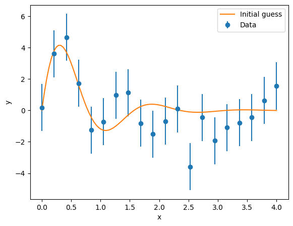
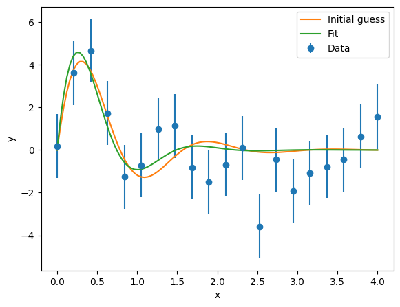
We assign this data to a Source, add the ExpSine model to this Source, and pass it to a Fitter to fit this. Since this requires a normal chisquare fit, no extra arguments are required for the fit.
datasource = satlas2.Source(data\_x, data\_y, yerr=yerr, name='Datafile1')
datasource.addModel(model)
f = satlas2.Fitter()
f.addSource(datasource)
f.fit()
print(f.reportFit())
fig = plt.figure()
ax = fig.add\_axes(\[0.1, 0.1, 0.8, 0.8\])
ax.errorbar(data\_x, data\_y, yerr=yerr, fmt='o', label='Data')
ax.plot(x, y, label='Initial guess')
ax.plot(x, model.f(x), label='Fit')
ax.set\_xlabel('x')
ax.set\_ylabel('y')
ax.legend(loc=0)
\[\[Fit Statistics\]\]
\# fitting method = leastsq
\# function evals = 93
\# data points = 20
\# variables = 3
chi\-square \= 14.1735643
reduced chi\-square \= 0.83373907
Akaike info crit \= \-0.88707432
Bayesian info crit \= 2.10012250
\[\[Variables\]\]
Datafile1\_\_\_MyModel\_\_\_amplitude: 9.03884096 +/- 4.31842559 (47.78%) (init \= 7)
Datafile1\_\_\_MyModel\_\_\_lambda: 2.15722712 +/- 1.22083220 (56.59%) (init \= 1.5)
Datafile1\_\_\_MyModel\_\_\_omega: 4.22415871 +/- 0.68336353 (16.18%) (init \= 4)
Contents
---
# Extracting dataframes — SATLAS2
[Skip to main content](https://iks-nm.github.io/satlas2/tutorials/dataframe/index.html#main-content)
Back to top Ctrl+K
[ \
\
SATLAS2](https://iks-nm.github.io/satlas2/index.html)
Search Ctrl+K
* [Repository](https://github.com/iks-nm/satlas2)
* [Suggest edit](https://github.com/iks-nm/satlas2/edit/master/tutorials/dataframe/index.rst)
* [Open issue](https://github.com/iks-nm/satlas2/issues/new?title=Issue%20on%20page%20%2Ftutorials/dataframe/index.html&body=Your%20issue%20content%20here.)
* [.rst](https://iks-nm.github.io/satlas2/_sources/tutorials/dataframe/index.rst)
* .pdf
Light Dark System Settings
Extracting dataframes
=====================
Extracting dataframes[#](https://iks-nm.github.io/satlas2/tutorials/dataframe/index.html#extracting-dataframes "Permalink to this heading")
============================================================================================================================================
The results of a fit can be extracted from the Fitter object in the format of a Pandas DataFrame. Aside from the results themselves, the additional statistics from the fitting can also be extracted in a separate DataFrame.
This will be demonstrated by fitting multiple spectra of a Voigt peak on top of an exponential background:
import sys
sys.path.insert(0, '..\\src')
from io import BytesIO
import matplotlib.pyplot as plt
import numpy as np
import pandas as pd
import satlas2
def modifiedSqrt(input):
output = np.sqrt(input)
output\[input <= 0\] = 1
return output
def createModels(backg, lamda, loc, fwhmg, fwhml, amp):
bkg = satlas2.ExponentialDecay(backg, lamda, name='Background')
peak = satlas2.Voigt(amp, loc, fwhmg, fwhml, name='Signal')
return peak, bkg
Defining the parameters and preparing the needed arrays for saving the results:
loc = 500
fwhmg = 150
fwhml = 150
amp = 200
bkg1 = 1000
bkg2 = 500
bkg3 = 700
lamda = 500
rng = np.random.default\_rng(0)
x = np.linspace(0, 1000, 250)
bkgs = \[bkg1, bkg2, bkg3\]
names = \['Scan1', 'Scan2', 'Scan3'\]
metadata = \[\]
results = \[\]
imgdatas = \[\]
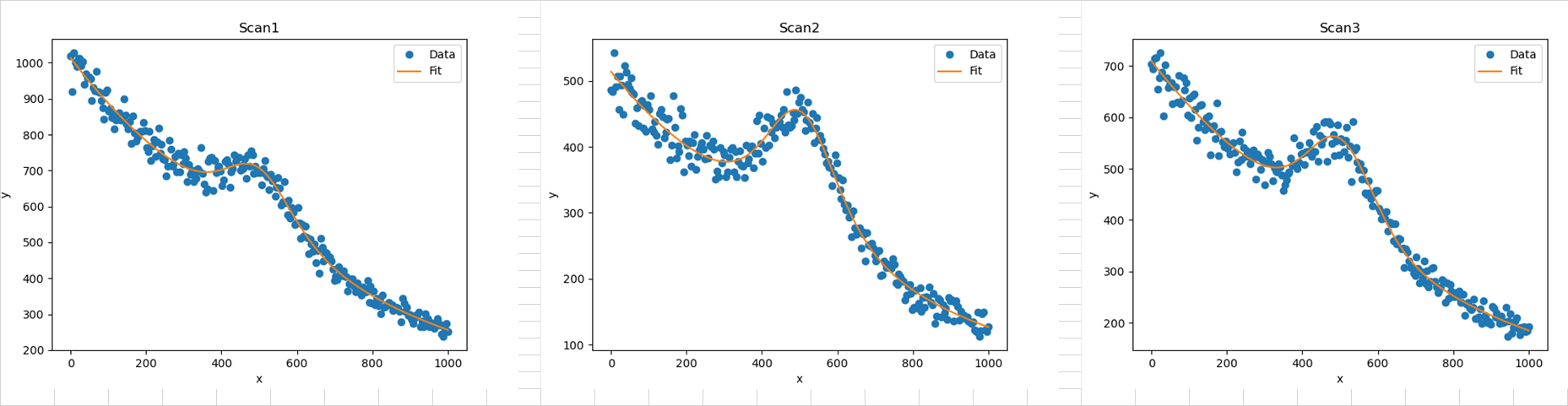
In a loop, generate three different datasets and fit them separately. The plots are saved to a BytesIO object for saving to an Excel spreadsheet later.
for bkg, name in zip(bkgs, names):
peakm, bkgm = createModels(bkg, lamda, loc, fwhmg, fwhml, amp)
y = satlas2.generateSpectrum(\[peakm, bkgm\], x, rng.poisson)
fig = plt.figure()
ax = fig.add\_axes(\[0.1, 0.1, 0.8, 0.8\])
ax.plot(x, y, 'o', label='Data')
ax.set\_xlabel('x')
ax.set\_ylabel('y')
datasource = satlas2.Source(x, y, yerr=modifiedSqrt, name=name)
datasource.addModel(peakm)
datasource.addModel(bkgm)
f = satlas2.Fitter()
f.addSource(datasource)
f.fit()
ax.plot(datasource.x, datasource.f(), label='Fit')
ax.set\_title(name)
ax.legend(loc=0)
metadata.append(f.createMetadataDataframe())
results.append(f.createResultDataframe())
imgdata = BytesIO()
fig.savefig(imgdata, format='png')
imgdatas.append(imgdata)
metadata = pd.concat(metadata)
results = pd.concat(results)
The _metadata_ and _results_ DataFrames now contain the fitting statistics and parameter results of all three fits respectively. As an example of how this can be processed later, the DataFrames along with the plots will be saved to an Excel sheet in the following section:
filename = 'test.xlsx'
figwidth = 10 # Standard figure size is about 10 cells
with pd.ExcelWriter(filename, engine='xlsxwriter') as writer:
metadata.to\_excel(writer, sheet\_name='Metadata', index=False)
results.to\_excel(writer, sheet\_name='Results', index=False)
workbook = writer.book
red\_format = workbook.add\_format({
'bg\_color': '#FFC7CE',
'font\_color': '#9C0006'
})
green\_format = workbook.add\_format({
'bg\_color': '#C6EFCE',
'font\_color': '#006100'
})
yellow\_format = workbook.add\_format({
'bg\_color': '#FFEB9C',
'font\_color': '#9C5700'
})
metadatasheet = workbook.get\_worksheet\_by\_name('Metadata')
resultssheet = workbook.get\_worksheet\_by\_name('Results')
figuressheet = workbook.add\_worksheet('Figures')
for i, im in enumerate(imgdatas):
im.seek(0)
figuressheet.insert\_image(0, 0 + i \* 10, "", {'image\_data': im})
# Add conditional formatting to illustrate reduced chisquares that
# are above the 1-sigma estimate for the reduced chisquare
metadatasheet.conditional\_format(
'H2:H99', {
'type': 'cell',
'criteria': 'not between',
'minimum': '=1-SQRT(2/(E2:E99-F2:F99))',
'maximum': '=1+SQRT(2/(E2:E99-F2:F99))',
'format': yellow\_format
})
metadatasheet.conditional\_format(
'H2:H99', {
'type': 'cell',
'criteria': 'between',
'minimum': '=1-SQRT(2/(E2:E99-F2:F99))',
'maximum': '=1+SQRT(2/(E2:E99-F2:F99))',
'format': green\_format
})
try:
metadatasheet.autofit()
resultssheet.autofit()
except:
pass
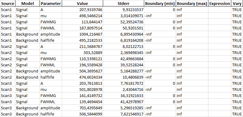
This results in an Excel sheet with the first sheet looking like this:

The second sheet contains the parameter results:
And the third sheet contains figures of the three datasets:
---
# Different emcee moves — SATLAS2
[Skip to main content](https://iks-nm.github.io/satlas2/tutorials/walkoptions/index.html#main-content)
Back to top Ctrl+K
[ \
\
SATLAS2](https://iks-nm.github.io/satlas2/index.html)
Search Ctrl+K
* [Repository](https://github.com/iks-nm/satlas2)
* [Suggest edit](https://github.com/iks-nm/satlas2/edit/master/tutorials/walkoptions/index.rst)
* [Open issue](https://github.com/iks-nm/satlas2/issues/new?title=Issue%20on%20page%20%2Ftutorials/walkoptions/index.html&body=Your%20issue%20content%20here.)
* [.rst](https://iks-nm.github.io/satlas2/_sources/tutorials/walkoptions/index.rst)
* .pdf
Light Dark System Settings
Different emcee moves
=====================
Contents
--------
Different `emcee` moves[#](https://iks-nm.github.io/satlas2/tutorials/walkoptions/index.html#different-emcee-moves "Permalink to this heading")
================================================================================================================================================
The `emcee` library that is used for the random walk exploration of the parameter space has some options that are exposed in the SATLAS2 interface. One interesting option is the ability to change the algorithms used to propose moves. The `emcee` documentation contains a tutorial on how and why different moves can be used [here](https://emcee.readthedocs.io/en/stable/tutorials/moves/)
.
The exploration of the parameter space for hyperfine spectra does benefit from this option. The difference between the standard stretch move and the proposed mix of differential evolution move and snooker move will be explored.
import sys
import time
import emcee
import matplotlib.gridspec as gridspec
import matplotlib.pyplot as plt
import numpy as np
sys.path.insert(0, '..\\..\\..\\src')
import satlas2
def modifiedSqrt(input):
output = np.sqrt(input)
output\[input <= 0\] = 1
return output
Data generation[#](https://iks-nm.github.io/satlas2/tutorials/walkoptions/index.html#data-generation "Permalink to this heading")
----------------------------------------------------------------------------------------------------------------------------------
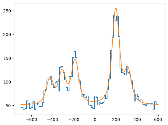
The convenience function included in SATLAS2 is used to generate a Poisson distributed spectrum.
A = \[50, 250\]
B = \[10, 5\]
C = \[0, 0\]
I = 1.0
J = \[1.0, 1.0\]
df = 0
fwhmg = 50
fwhml = 50
scale = 200
bkg = 50
hfs = satlas2.HFS(I, J, A=A, B=B, C=C, df=df, fwhmg=fwhmg, fwhml=fwhml, scale=scale)
bkg = satlas2.Polynomial(\[bkg\])
x = np.linspace(-700, 600, 1000)
data\_x = np.arange(x.min(), x.max(), 15)
data\_y = satlas2.generateSpectrum(\[hfs, bkg\], data\_x)
plt.plot(data\_x, data\_y, drawstyle='steps-mid')
plt.plot(x, hfs.f(x)+bkg.f(x))
f = satlas2.Fitter()
datasource = satlas2.Source(data\_x, data\_y, yerr=modifiedSqrt, name='Artificial')
datasource.addModel(hfs)
datasource.addModel(bkg)
f.addSource(datasource)
f.fit()
print(f.reportFit())
\[\[Fit Statistics\]\]
\# fitting method = leastsq
\# function evals = 91
\# data points = 87
\# variables = 9
chi\-square \= 72.8990076
reduced chi\-square \= 0.93460266
Akaike info crit \= 2.61552097
Bayesian info crit \= 24.8086940
\[\[Variables\]\]
Artificial\_\_\_HFS\_\_\_centroid: \-0.37055045 +/- 1.42164523 (383.66%) (init \= 0)
Artificial\_\_\_HFS\_\_\_Al: 51.4477619 +/- 1.39705770 (2.72%) (init \= 50)
Artificial\_\_\_HFS\_\_\_Au: 251.236334 +/- 1.65652941 (0.66%) (init \= 250)
Artificial\_\_\_HFS\_\_\_Bl: 12.5419832 +/- 2.59229524 (20.67%) (init \= 10)
Artificial\_\_\_HFS\_\_\_Bu: 4.34080560 +/- 1.74164467 (40.12%) (init \= 5)
Artificial\_\_\_HFS\_\_\_Cl: 0 (fixed)
Artificial\_\_\_HFS\_\_\_Cu: 0 (fixed)
Artificial\_\_\_HFS\_\_\_FWHMG: 56.0066443 +/- 10.2656213 (18.33%) (init \= 50)
Artificial\_\_\_HFS\_\_\_FWHML: 42.4534449 +/- 11.2048829 (26.39%) (init \= 50)
Artificial\_\_\_HFS\_\_\_scale: 205.225337 +/- 7.32534024 (3.57%) (init \= 200)
Artificial\_\_\_HFS\_\_\_Amp0to1: 0.2666667 (fixed)
Artificial\_\_\_HFS\_\_\_Amp1to0: 0.2666667 (fixed)
Artificial\_\_\_HFS\_\_\_Amp1to1: 0.2 (fixed)
Artificial\_\_\_HFS\_\_\_Amp1to2: 0.3333333 (fixed)
Artificial\_\_\_HFS\_\_\_Amp2to1: 0.3333333 (fixed)
Artificial\_\_\_HFS\_\_\_Amp2to2: 1 (fixed)
Artificial\_\_\_Polynomial\_\_\_p0: 48.4270596 +/- 1.97001650 (4.07%) (init \= 50)
Standard `emcee` move[#](https://iks-nm.github.io/satlas2/tutorials/walkoptions/index.html#standard-emcee-move "Permalink to this heading")
--------------------------------------------------------------------------------------------------------------------------------------------
The normal move used by `emcee` is called the StretchMove, and is used by not specifying any specific moves at all
stretchfile = 'stretchmove.h5'
f.fit(method='emcee', filename=stretchfile)
100%|████████████| 1000/1000 \[00:28<00:00, 35.70it/s\]
The chain is shorter than 50 times the integrated autocorrelation time for 9 parameter(s). Use this estimate with caution and run a longer chain!
N/50 = 20;
tau: \[52.18497247 57.73151625 50.61482182 58.94721213 55.18218592 53.97033804\
51.2988931 56.19765179 49.45745584\]
The warning here shows that, in order to get good estimates, more samples are recommended. For more information, see the `emcee` documentation. However, the important detail here is the list of autocorrelation times that is estimated here, which is about 50-60 steps.
fig, axes = satlas2.generateWalkPlot(stretchfile)
fig.set\_size\_inches(6, 10)
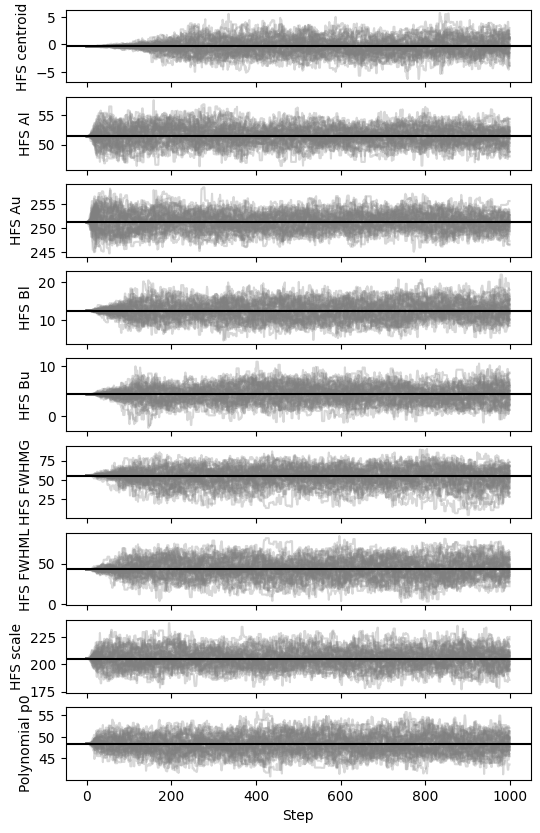
Here, the burn-in is quite long for several parameters. If possible, avoiding long burn-ins is very useful to increase useful computation time.
Using differential evolution moves[#](https://iks-nm.github.io/satlas2/tutorials/walkoptions/index.html#using-differential-evolution-moves "Permalink to this heading")
------------------------------------------------------------------------------------------------------------------------------------------------------------------------
Starting from version 3, `emcee` has a Moves interface where the proposal for the random walk can be changed. In addition to specifying another algorithm, a selection of moves can be given along with a float that represents the chance the algorithm is selected. Giving an ensemble of move proposals in this way can improve overall performance.
As illustrated in the linked documentation, a combination of DEMove and DESnookerMove can perform better in highly dimensional or lightly multimodal distributions. Both of these descriptions can be well applied to the fitting of hyperfine spectra.
combinationfile = 'combination.h5'
f.revertFit()
f.fit(method='emcee', filename=combinationfile, sampler\_kwargs={'moves': \[\
(emcee.moves.DEMove(), 0.8),\
(emcee.moves.DESnookerMove(), 0.2)\
\]})
100%|████████████| 1000/1000 \[00:28<00:00, 35.65it/s\]
The chain is shorter than 50 times the integrated autocorrelation time for 9 parameter(s). Use this estimate with caution and run a longer chain!
N/50 = 20;
tau: \[25.79202768 28.04787132 31.15895649 27.02757601 27.06688899 32.62843194\
33.30301554 29.44226374 30.75024705\]
As with the previous case, the recommendation is that a longer chain is used. However, the autocorrelation time is much shorter, 20-30 steps instead of the previous 50-60 steps. This corresponds to a walk that shows a much lower burn-in time.
fig, axes = satlas2.generateWalkPlot(combinationfile)
fig.set\_size\_inches(6, 10)
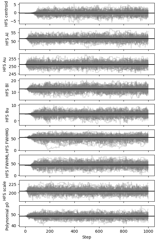
This is clearly reflected in the resulting walk. Experimentation with the exact mixture of Moves can result in even better performance. Since SATLAS2 relies on the interface provided by emcee, any future Moves that are introduced can automatically be used in SATLAS2 for sampling.
Contents
---
# Benchmark of SATLAS2 speed — SATLAS2
[Skip to main content](https://iks-nm.github.io/satlas2/tutorials/benchmark/index.html#main-content)
Back to top Ctrl+K
[ \
\
SATLAS2](https://iks-nm.github.io/satlas2/index.html)
Search Ctrl+K
* [Repository](https://github.com/iks-nm/satlas2)
* [Suggest edit](https://github.com/iks-nm/satlas2/edit/master/tutorials/benchmark/index.rst)
* [Open issue](https://github.com/iks-nm/satlas2/issues/new?title=Issue%20on%20page%20%2Ftutorials/benchmark/index.html&body=Your%20issue%20content%20here.)
* [.rst](https://iks-nm.github.io/satlas2/_sources/tutorials/benchmark/index.rst)
* .pdf
Light Dark System Settings
Benchmark of SATLAS2 speed
==========================
Benchmark of SATLAS2 speed[#](https://iks-nm.github.io/satlas2/tutorials/benchmark/index.html#benchmark-of-satlas2-speed "Permalink to this heading")
======================================================================================================================================================
The simultaneous fit of sets of data is shown in this notebook. The data generation code can be replaced by code that reads in datafiles, so this script can serve as the basis for your own analysis. The fitting is compared to the simulatenous fit in the first version of satlas.
First, start with an import of all the relevant libraries:
import sys
import time
import matplotlib.gridspec as gridspec
import matplotlib.pyplot as plt
import numpy as np
sys.path.insert(0, '..\\src')
import satlas2
import satlas as sat
Define a modified root function to handle uncertainties of 0 counts in a Poisson statistic
def modifiedSqrt(input):
output = np.sqrt(input)
output\[input <= 0\] = 1
return output
Define all the parameters and, in a for-loop, define the HFS and background models to generate the data from. The fitting already occurs inside the for loop, so the performance can be seen as a function of the number of datasets that are being analysed.
spin = 3.5
J = \[0.5, 1.5\]
A = \[9600, 175\]
B = \[0, 315\]
C = \[0, 0\]
FWHMG = 135
FWHML = 101
centroid = 480
bkg = 10
scale = 90
x = np.arange(-17500, -14500, 40)
x = np.hstack(\[x, np.arange(20000, 23000, 40)\])
times = \[\]
times\_1 = \[\]
rng = np.random.default\_rng(0)
for j in range(1, 11):
f = satlas2.Fitter()
models = \[\]
X = \[\]
Y = \[\]
for i in range(j):
hfs = satlas2.HFS(spin,
J,
A=A,
B=B,
C=C,
scale=scale,
df=centroid,
name='HFS1',
racah=True,
fwhmg=135,
fwhml=100)
bkgm = satlas2.Polynomial(\[bkg\], name='bkg1')
y = satlas2.generateSpectrum(\[hfs, bkgm\], x, rng.poisson)
hfs.params\['centroid'\].value = centroid - 100
X.append(x)
Y.append(y)
hfs1 = sat.HFSModel(spin,
J,
\[A\[0\], A\[1\], B\[0\], B\[1\], C\[0\], C\[1\]\],
centroid - 100, \[FWHMG, FWHML\],
scale=scale,
background\_params=\[bkg\],
use\_racah=True)
models.append(hfs1)
datasource = satlas2.Source(x,
y,
yerr=modifiedSqrt,
name='Scan{}'.format(i + 1))
datasource.addModel(hfs)
datasource.addModel(bkgm)
f.addSource(datasource)
share = \['Al', 'Au', 'Bl', 'centroid', 'FWHMG', 'FWHML'\]
m = sat.LinkedModel(models)
m.shared = share
f.shareModelParams(share)
print('Fitting {} datasets with chisquare (Pearson, satlas2)...'.format(j))
start = time.time()
f.fit()
stop = time.time()
dt = stop - start
print('{:.3} s, {:.0f} function evaluations'.format(dt, f.result.nfev))
times.append(dt)
print('Fitting {} datasets with chisquare (Pearson, satlas1)...'.format(j))
start = time.time()
sat.chisquare\_spectroscopic\_fit(m, X, Y)
stop = time.time()
dt = stop - start
times\_1.append(dt)
fig = plt.figure()
ax = fig.add\_axes(\[0.1, 0.1, 0.8, 0.8\])
ax.plot(range(1, len(times) + 1), times, '-o', label='satlas2')
ax.plot(range(1, len(times\_1) + 1), times\_1, '-o', label='satlas1')
ax.set\_xlabel('Number of datasets')
ax.set\_ylabel('Fitting time in seconds')
ax.set\_yscale('log')
ax.legend(loc=0)
times, times\_1 = np.array(times), np.array(times\_1)
fig = plt.figure()
ax = fig.add\_axes(\[0.1, 0.1, 0.8, 0.8\])
ax.plot(range(1, len(times) + 1), times\_1/times, '-o')
ax.set\_xlabel('Number of datasets')
ax.set\_ylabel('Speedup factor by using satlas2')
Fitting 1 datasets with chisquare (Pearson, satlas2)...
0.041 s, 73 function evaluations
Fitting 1 datasets with chisquare (Pearson, satlas1)...
Chisquare fitting done: 98it \[00:00, 100.10it/s\]
Fitting 2 datasets with chisquare (Pearson, satlas2)...
0.102 s, 110 function evaluations
Fitting 2 datasets with chisquare (Pearson, satlas1)...
Chisquare fitting done: 174it \[00:05, 30.77it/s\]
Fitting 3 datasets with chisquare (Pearson, satlas2)...
0.154 s, 122 function evaluations
Fitting 3 datasets with chisquare (Pearson, satlas1)...
Chisquare fitting done: 209it \[00:14, 14.83it/s\]
Fitting 4 datasets with chisquare (Pearson, satlas2)...
0.278 s, 163 function evaluations
Fitting 4 datasets with chisquare (Pearson, satlas1)...
Chisquare fitting in progress (516.8577280066263): 258it \[00:29, 8.60it/s\]
Fitting 5 datasets with chisquare (Pearson, satlas2)...
0.365 s, 169 function evaluations
Fitting 5 datasets with chisquare (Pearson, satlas1)...
Chisquare fitting in progress (791.4835074105964): 308it \[00:54, 5.90it/s\]
Fitting 6 datasets with chisquare (Pearson, satlas2)...
0.521 s, 217 function evaluations
Fitting 6 datasets with chisquare (Pearson, satlas1)...
Chisquare fitting in progress (921.0408291264894): 393it \[01:39, 3.97it/s\]
Fitting 7 datasets with chisquare (Pearson, satlas2)...
0.702 s, 244 function evaluations
Fitting 7 datasets with chisquare (Pearson, satlas1)...
Chisquare fitting in progress (1025.7328760442326): 448it \[02:34, 2.88it/s\]
Fitting 8 datasets with chisquare (Pearson, satlas2)...
0.929 s, 271 function evaluations
Fitting 8 datasets with chisquare (Pearson, satlas1)...
Chisquare fitting in progress (1116.8718639445108): 458it \[03:23, 2.33it/s\]
Fitting 9 datasets with chisquare (Pearson, satlas2)...
1.09 s, 298 function evaluations
Fitting 9 datasets with chisquare (Pearson, satlas1)...
Chisquare fitting in progress (1254.023933377538): 558it \[05:11, 1.77it/s\]
Fitting 10 datasets with chisquare (Pearson, satlas2)...
1.23 s, 290 function evaluations
Fitting 10 datasets with chisquare (Pearson, satlas1)...
Chisquare fitting in progress (1406.051401654012): 559it \[06:16, 1.50it/s\]
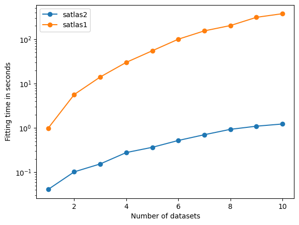 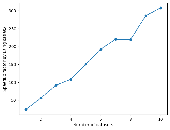
Plot the fit result, then revert the fit to show the initial starting condition of the spectrum.
fig = plt.figure(constrained\_layout=True)
gs = gridspec.GridSpec(nrows=len(f.sources), ncols=2, figure=fig)
a1 = None
a2 = None
axes = \[\]
for i, (name, datasource) in enumerate(f.sources):
if a1 is None:
ax1 = fig.add\_subplot(gs\[i, 0\])
ax2 = fig.add\_subplot(gs\[i, 1\])
a1 = ax1
a2 = ax2
else:
ax1 = fig.add\_subplot(gs\[i, 0\], sharex=a1)
ax2 = fig.add\_subplot(gs\[i, 1\], sharex=a2)
left = datasource.x < 0
right = datasource.x > 0
smooth\_left = np.arange(datasource.x\[left\].min(), datasource.x\[left\].max(),
5.0)
smooth\_right = np.arange(datasource.x\[right\].min(),
datasource.x\[right\].max(), 5.0)
ax1.plot(datasource.x\[left\],
datasource.y\[left\],
drawstyle='steps-mid',
label='Data')
ax1.plot(smooth\_left, datasource.evaluate(smooth\_left), label='Fit')
ax2.plot(datasource.x\[right\],
datasource.y\[right\],
drawstyle='steps-mid',
label='Data')
ax2.plot(smooth\_right, datasource.evaluate(smooth\_right), label='Fit')
ax1.set\_xlabel('Frequency \[MHz\]')
ax2.set\_xlabel('Frequency \[MHz\]')
ax1.set\_ylabel('Counts')
ax2.set\_ylabel('Counts')
ax1.label\_outer()
ax2.label\_outer()
axes.append(\[ax1, ax2\])
f.revertFit()
for i, (name, datasource) in enumerate(f.sources):
smooth\_left = np.arange(datasource.x\[left\].min(), datasource.x\[left\].max(),
5.0)
smooth\_right = np.arange(datasource.x\[right\].min(),
datasource.x\[right\].max(), 5.0)
axes\[i\]\[0\].plot(smooth\_left, datasource.evaluate(smooth\_left), label='Initial')
axes\[i\]\[1\].plot(smooth\_right,
datasource.evaluate(smooth\_right),
label='Initial')
a1.legend(loc=0)
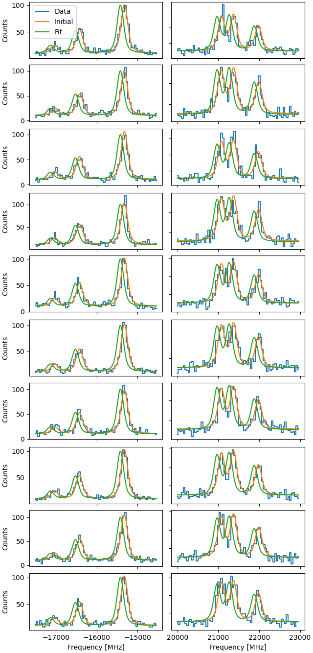
print(f.reportFit())
\[\[Fit Statistics\]\]
\# fitting method = leastsq
\# function evals = 290
\# data points = 1500
\# variables = 35
chi\-square \= 1423.58804
reduced chi\-square \= 0.97173245
Akaike info crit \= \-8.42695240
Bayesian info crit \= 177.535761
\[\[Variables\]\]
Scan1\_\_\_HFS1\_\_\_centroid: 481.497549 +/- 1.15593654 (0.24%) (init \= 380)
Scan1\_\_\_HFS1\_\_\_Al: 9600.61046 +/- 0.92670540 (0.01%) (init \= 9600)
Scan1\_\_\_HFS1\_\_\_Au: 174.571911 +/- 0.40166968 (0.23%) (init \= 175)
Scan1\_\_\_HFS1\_\_\_Bl: 0 (fixed)
Scan1\_\_\_HFS1\_\_\_Bu: 316.727852 +/- 9.58185930 (3.03%) (init \= 315)
Scan1\_\_\_HFS1\_\_\_Cl: 0 (fixed)
Scan1\_\_\_HFS1\_\_\_Cu: 0 (fixed)
Scan1\_\_\_HFS1\_\_\_FWHMG: 130.719040 +/- 8.12890265 (6.22%) (init \= 135)
Scan1\_\_\_HFS1\_\_\_FWHML: 105.176292 +/- 7.66248618 (7.29%) (init \= 100)
Scan1\_\_\_HFS1\_\_\_scale: 90.9386339 +/- 3.18982406 (3.51%) (init \= 90)
Scan1\_\_\_HFS1\_\_\_Amp3to2: 0.4545455 (fixed)
Scan1\_\_\_HFS1\_\_\_Amp3to3: 0.4772727 (fixed)
Scan1\_\_\_HFS1\_\_\_Amp3to4: 0.3409091 (fixed)
Scan1\_\_\_HFS1\_\_\_Amp4to3: 0.1590909 (fixed)
Scan1\_\_\_HFS1\_\_\_Amp4to4: 0.4772727 (fixed)
Scan1\_\_\_HFS1\_\_\_Amp4to5: 1 (fixed)
Scan1\_\_\_bkg1\_\_\_p0: 10.2241495 +/- 0.38793282 (3.79%) (init \= 10)
Scan2\_\_\_HFS1\_\_\_centroid: 481.497549 +/- 1.15593654 (0.24%) \== 'Scan1\_\_\_HFS1\_\_\_centroid'
Scan2\_\_\_HFS1\_\_\_Al: 9600.61046 +/- 0.92670540 (0.01%) \== 'Scan1\_\_\_HFS1\_\_\_Al'
Scan2\_\_\_HFS1\_\_\_Au: 174.571911 +/- 0.40166968 (0.23%) \== 'Scan1\_\_\_HFS1\_\_\_Au'
Scan2\_\_\_HFS1\_\_\_Bl: 0.00000000 +/- 0.00000000 \== 'Scan1\_\_\_HFS1\_\_\_Bl'
Scan2\_\_\_HFS1\_\_\_Bu: 301.516120 +/- 9.76476582 (3.24%) (init \= 315)
Scan2\_\_\_HFS1\_\_\_Cl: 0 (fixed)
Scan2\_\_\_HFS1\_\_\_Cu: 0 (fixed)
Scan2\_\_\_HFS1\_\_\_FWHMG: 130.719040 +/- 8.12890268 (6.22%) \== 'Scan1\_\_\_HFS1\_\_\_FWHMG'
Scan2\_\_\_HFS1\_\_\_FWHML: 105.176292 +/- 7.66248618 (7.29%) \== 'Scan1\_\_\_HFS1\_\_\_FWHML'
Scan2\_\_\_HFS1\_\_\_scale: 88.4215797 +/- 3.18866686 (3.61%) (init \= 90)
Scan2\_\_\_HFS1\_\_\_Amp3to2: 0.4545455 (fixed)
Scan2\_\_\_HFS1\_\_\_Amp3to3: 0.4772727 (fixed)
Scan2\_\_\_HFS1\_\_\_Amp3to4: 0.3409091 (fixed)
Scan2\_\_\_HFS1\_\_\_Amp4to3: 0.1590909 (fixed)
Scan2\_\_\_HFS1\_\_\_Amp4to4: 0.4772727 (fixed)
Scan2\_\_\_HFS1\_\_\_Amp4to5: 1 (fixed)
Scan2\_\_\_bkg1\_\_\_p0: 10.7465561 +/- 0.39604567 (3.69%) (init \= 10)
Scan3\_\_\_HFS1\_\_\_centroid: 481.497549 +/- 1.15593654 (0.24%) \== 'Scan1\_\_\_HFS1\_\_\_centroid'
Scan3\_\_\_HFS1\_\_\_Al: 9600.61046 +/- 0.92670540 (0.01%) \== 'Scan1\_\_\_HFS1\_\_\_Al'
Scan3\_\_\_HFS1\_\_\_Au: 174.571911 +/- 0.40166968 (0.23%) \== 'Scan1\_\_\_HFS1\_\_\_Au'
Scan3\_\_\_HFS1\_\_\_Bl: 0.00000000 +/- 0.00000000 \== 'Scan1\_\_\_HFS1\_\_\_Bl'
Scan3\_\_\_HFS1\_\_\_Bu: 316.467273 +/- 9.15709217 (2.89%) (init \= 315)
Scan3\_\_\_HFS1\_\_\_Cl: 0 (fixed)
Scan3\_\_\_HFS1\_\_\_Cu: 0 (fixed)
Scan3\_\_\_HFS1\_\_\_FWHMG: 130.719040 +/- 8.12890268 (6.22%) \== 'Scan1\_\_\_HFS1\_\_\_FWHMG'
Scan3\_\_\_HFS1\_\_\_FWHML: 105.176292 +/- 7.66248618 (7.29%) \== 'Scan1\_\_\_HFS1\_\_\_FWHML'
Scan3\_\_\_HFS1\_\_\_scale: 95.8064722 +/- 3.27951355 (3.42%) (init \= 90)
Scan3\_\_\_HFS1\_\_\_Amp3to2: 0.4545455 (fixed)
Scan3\_\_\_HFS1\_\_\_Amp3to3: 0.4772727 (fixed)
Scan3\_\_\_HFS1\_\_\_Amp3to4: 0.3409091 (fixed)
Scan3\_\_\_HFS1\_\_\_Amp4to3: 0.1590909 (fixed)
Scan3\_\_\_HFS1\_\_\_Amp4to4: 0.4772727 (fixed)
Scan3\_\_\_HFS1\_\_\_Amp4to5: 1 (fixed)
Scan3\_\_\_bkg1\_\_\_p0: 10.3773605 +/- 0.39449044 (3.80%) (init \= 10)
Scan4\_\_\_HFS1\_\_\_centroid: 481.497549 +/- 1.15593654 (0.24%) \== 'Scan1\_\_\_HFS1\_\_\_centroid'
Scan4\_\_\_HFS1\_\_\_Al: 9600.61046 +/- 0.92670540 (0.01%) \== 'Scan1\_\_\_HFS1\_\_\_Al'
Scan4\_\_\_HFS1\_\_\_Au: 174.571911 +/- 0.40166968 (0.23%) \== 'Scan1\_\_\_HFS1\_\_\_Au'
Scan4\_\_\_HFS1\_\_\_Bl: 0.00000000 +/- 0.00000000 \== 'Scan1\_\_\_HFS1\_\_\_Bl'
Scan4\_\_\_HFS1\_\_\_Bu: 306.363833 +/- 9.44073795 (3.08%) (init \= 315)
Scan4\_\_\_HFS1\_\_\_Cl: 0 (fixed)
Scan4\_\_\_HFS1\_\_\_Cu: 0 (fixed)
Scan4\_\_\_HFS1\_\_\_FWHMG: 130.719040 +/- 8.12890268 (6.22%) \== 'Scan1\_\_\_HFS1\_\_\_FWHMG'
Scan4\_\_\_HFS1\_\_\_FWHML: 105.176292 +/- 7.66248618 (7.29%) \== 'Scan1\_\_\_HFS1\_\_\_FWHML'
Scan4\_\_\_HFS1\_\_\_scale: 91.9771725 +/- 3.22329550 (3.50%) (init \= 90)
Scan4\_\_\_HFS1\_\_\_Amp3to2: 0.4545455 (fixed)
Scan4\_\_\_HFS1\_\_\_Amp3to3: 0.4772727 (fixed)
Scan4\_\_\_HFS1\_\_\_Amp3to4: 0.3409091 (fixed)
Scan4\_\_\_HFS1\_\_\_Amp4to3: 0.1590909 (fixed)
Scan4\_\_\_HFS1\_\_\_Amp4to4: 0.4772727 (fixed)
Scan4\_\_\_HFS1\_\_\_Amp4to5: 1 (fixed)
Scan4\_\_\_bkg1\_\_\_p0: 10.8933956 +/- 0.39725280 (3.65%) (init \= 10)
Scan5\_\_\_HFS1\_\_\_centroid: 481.497549 +/- 1.15593654 (0.24%) \== 'Scan1\_\_\_HFS1\_\_\_centroid'
Scan5\_\_\_HFS1\_\_\_Al: 9600.61046 +/- 0.92670540 (0.01%) \== 'Scan1\_\_\_HFS1\_\_\_Al'
Scan5\_\_\_HFS1\_\_\_Au: 174.571911 +/- 0.40166968 (0.23%) \== 'Scan1\_\_\_HFS1\_\_\_Au'
Scan5\_\_\_HFS1\_\_\_Bl: 0.00000000 +/- 0.00000000 \== 'Scan1\_\_\_HFS1\_\_\_Bl'
Scan5\_\_\_HFS1\_\_\_Bu: 311.300307 +/- 9.57352553 (3.08%) (init \= 315)
Scan5\_\_\_HFS1\_\_\_Cl: 0 (fixed)
Scan5\_\_\_HFS1\_\_\_Cu: 0 (fixed)
Scan5\_\_\_HFS1\_\_\_FWHMG: 130.719040 +/- 8.12890268 (6.22%) \== 'Scan1\_\_\_HFS1\_\_\_FWHMG'
Scan5\_\_\_HFS1\_\_\_FWHML: 105.176292 +/- 7.66248618 (7.29%) \== 'Scan1\_\_\_HFS1\_\_\_FWHML'
Scan5\_\_\_HFS1\_\_\_scale: 90.7998344 +/- 3.20100095 (3.53%) (init \= 90)
Scan5\_\_\_HFS1\_\_\_Amp3to2: 0.4545455 (fixed)
Scan5\_\_\_HFS1\_\_\_Amp3to3: 0.4772727 (fixed)
Scan5\_\_\_HFS1\_\_\_Amp3to4: 0.3409091 (fixed)
Scan5\_\_\_HFS1\_\_\_Amp4to3: 0.1590909 (fixed)
Scan5\_\_\_HFS1\_\_\_Amp4to4: 0.4772727 (fixed)
Scan5\_\_\_HFS1\_\_\_Amp4to5: 1 (fixed)
Scan5\_\_\_bkg1\_\_\_p0: 10.3707148 +/- 0.39092416 (3.77%) (init \= 10)
Scan6\_\_\_HFS1\_\_\_centroid: 481.497549 +/- 1.15593654 (0.24%) \== 'Scan1\_\_\_HFS1\_\_\_centroid'
Scan6\_\_\_HFS1\_\_\_Al: 9600.61046 +/- 0.92670540 (0.01%) \== 'Scan1\_\_\_HFS1\_\_\_Al'
Scan6\_\_\_HFS1\_\_\_Au: 174.571911 +/- 0.40166968 (0.23%) \== 'Scan1\_\_\_HFS1\_\_\_Au'
Scan6\_\_\_HFS1\_\_\_Bl: 0.00000000 +/- 0.00000000 \== 'Scan1\_\_\_HFS1\_\_\_Bl'
Scan6\_\_\_HFS1\_\_\_Bu: 313.188923 +/- 9.22636900 (2.95%) (init \= 315)
Scan6\_\_\_HFS1\_\_\_Cl: 0 (fixed)
Scan6\_\_\_HFS1\_\_\_Cu: 0 (fixed)
Scan6\_\_\_HFS1\_\_\_FWHMG: 130.719040 +/- 8.12890268 (6.22%) \== 'Scan1\_\_\_HFS1\_\_\_FWHMG'
Scan6\_\_\_HFS1\_\_\_FWHML: 105.176292 +/- 7.66248618 (7.29%) \== 'Scan1\_\_\_HFS1\_\_\_FWHML'
Scan6\_\_\_HFS1\_\_\_scale: 92.7961475 +/- 3.20546516 (3.45%) (init \= 90)
Scan6\_\_\_HFS1\_\_\_Amp3to2: 0.4545455 (fixed)
Scan6\_\_\_HFS1\_\_\_Amp3to3: 0.4772727 (fixed)
Scan6\_\_\_HFS1\_\_\_Amp3to4: 0.3409091 (fixed)
Scan6\_\_\_HFS1\_\_\_Amp4to3: 0.1590909 (fixed)
Scan6\_\_\_HFS1\_\_\_Amp4to4: 0.4772727 (fixed)
Scan6\_\_\_HFS1\_\_\_Amp4to5: 1 (fixed)
Scan6\_\_\_bkg1\_\_\_p0: 9.85910281 +/- 0.38300602 (3.88%) (init \= 10)
Scan7\_\_\_HFS1\_\_\_centroid: 481.497549 +/- 1.15593654 (0.24%) \== 'Scan1\_\_\_HFS1\_\_\_centroid'
Scan7\_\_\_HFS1\_\_\_Al: 9600.61046 +/- 0.92670540 (0.01%) \== 'Scan1\_\_\_HFS1\_\_\_Al'
Scan7\_\_\_HFS1\_\_\_Au: 174.571911 +/- 0.40166968 (0.23%) \== 'Scan1\_\_\_HFS1\_\_\_Au'
Scan7\_\_\_HFS1\_\_\_Bl: 0.00000000 +/- 0.00000000 \== 'Scan1\_\_\_HFS1\_\_\_Bl'
Scan7\_\_\_HFS1\_\_\_Bu: 315.004090 +/- 10.1665755 (3.23%) (init \= 315)
Scan7\_\_\_HFS1\_\_\_Cl: 0 (fixed)
Scan7\_\_\_HFS1\_\_\_Cu: 0 (fixed)
Scan7\_\_\_HFS1\_\_\_FWHMG: 130.719040 +/- 8.12890268 (6.22%) \== 'Scan1\_\_\_HFS1\_\_\_FWHMG'
Scan7\_\_\_HFS1\_\_\_FWHML: 105.176292 +/- 7.66248618 (7.29%) \== 'Scan1\_\_\_HFS1\_\_\_FWHML'
Scan7\_\_\_HFS1\_\_\_scale: 87.2691437 +/- 3.12308461 (3.58%) (init \= 90)
Scan7\_\_\_HFS1\_\_\_Amp3to2: 0.4545455 (fixed)
Scan7\_\_\_HFS1\_\_\_Amp3to3: 0.4772727 (fixed)
Scan7\_\_\_HFS1\_\_\_Amp3to4: 0.3409091 (fixed)
Scan7\_\_\_HFS1\_\_\_Amp4to3: 0.1590909 (fixed)
Scan7\_\_\_HFS1\_\_\_Amp4to4: 0.4772727 (fixed)
Scan7\_\_\_HFS1\_\_\_Amp4to5: 1 (fixed)
Scan7\_\_\_bkg1\_\_\_p0: 10.3964797 +/- 0.38718000 (3.72%) (init \= 10)
Scan8\_\_\_HFS1\_\_\_centroid: 481.497549 +/- 1.15593654 (0.24%) \== 'Scan1\_\_\_HFS1\_\_\_centroid'
Scan8\_\_\_HFS1\_\_\_Al: 9600.61046 +/- 0.92670540 (0.01%) \== 'Scan1\_\_\_HFS1\_\_\_Al'
Scan8\_\_\_HFS1\_\_\_Au: 174.571911 +/- 0.40166968 (0.23%) \== 'Scan1\_\_\_HFS1\_\_\_Au'
Scan8\_\_\_HFS1\_\_\_Bl: 0.00000000 +/- 0.00000000 \== 'Scan1\_\_\_HFS1\_\_\_Bl'
Scan8\_\_\_HFS1\_\_\_Bu: 319.167680 +/- 9.49188859 (2.97%) (init \= 315)
Scan8\_\_\_HFS1\_\_\_Cl: 0 (fixed)
Scan8\_\_\_HFS1\_\_\_Cu: 0 (fixed)
Scan8\_\_\_HFS1\_\_\_FWHMG: 130.719040 +/- 8.12890268 (6.22%) \== 'Scan1\_\_\_HFS1\_\_\_FWHMG'
Scan8\_\_\_HFS1\_\_\_FWHML: 105.176292 +/- 7.66248618 (7.29%) \== 'Scan1\_\_\_HFS1\_\_\_FWHML'
Scan8\_\_\_HFS1\_\_\_scale: 92.6245328 +/- 3.20556643 (3.46%) (init \= 90)
Scan8\_\_\_HFS1\_\_\_Amp3to2: 0.4545455 (fixed)
Scan8\_\_\_HFS1\_\_\_Amp3to3: 0.4772727 (fixed)
Scan8\_\_\_HFS1\_\_\_Amp3to4: 0.3409091 (fixed)
Scan8\_\_\_HFS1\_\_\_Amp4to3: 0.1590909 (fixed)
Scan8\_\_\_HFS1\_\_\_Amp4to4: 0.4772727 (fixed)
Scan8\_\_\_HFS1\_\_\_Amp4to5: 1 (fixed)
Scan8\_\_\_bkg1\_\_\_p0: 10.1201224 +/- 0.38736226 (3.83%) (init \= 10)
Scan9\_\_\_HFS1\_\_\_centroid: 481.497549 +/- 1.15593654 (0.24%) \== 'Scan1\_\_\_HFS1\_\_\_centroid'
Scan9\_\_\_HFS1\_\_\_Al: 9600.61046 +/- 0.92670540 (0.01%) \== 'Scan1\_\_\_HFS1\_\_\_Al'
Scan9\_\_\_HFS1\_\_\_Au: 174.571911 +/- 0.40166968 (0.23%) \== 'Scan1\_\_\_HFS1\_\_\_Au'
Scan9\_\_\_HFS1\_\_\_Bl: 0.00000000 +/- 0.00000000 \== 'Scan1\_\_\_HFS1\_\_\_Bl'
Scan9\_\_\_HFS1\_\_\_Bu: 303.519268 +/- 9.25628071 (3.05%) (init \= 315)
Scan9\_\_\_HFS1\_\_\_Cl: 0 (fixed)
Scan9\_\_\_HFS1\_\_\_Cu: 0 (fixed)
Scan9\_\_\_HFS1\_\_\_FWHMG: 130.719040 +/- 8.12890268 (6.22%) \== 'Scan1\_\_\_HFS1\_\_\_FWHMG'
Scan9\_\_\_HFS1\_\_\_FWHML: 105.176292 +/- 7.66248618 (7.29%) \== 'Scan1\_\_\_HFS1\_\_\_FWHML'
Scan9\_\_\_HFS1\_\_\_scale: 94.8212808 +/- 3.23148508 (3.41%) (init \= 90)
Scan9\_\_\_HFS1\_\_\_Amp3to2: 0.4545455 (fixed)
Scan9\_\_\_HFS1\_\_\_Amp3to3: 0.4772727 (fixed)
Scan9\_\_\_HFS1\_\_\_Amp3to4: 0.3409091 (fixed)
Scan9\_\_\_HFS1\_\_\_Amp4to3: 0.1590909 (fixed)
Scan9\_\_\_HFS1\_\_\_Amp4to4: 0.4772727 (fixed)
Scan9\_\_\_HFS1\_\_\_Amp4to5: 1 (fixed)
Scan9\_\_\_bkg1\_\_\_p0: 9.99299420 +/- 0.38760703 (3.88%) (init \= 10)
Scan10\_\_\_HFS1\_\_\_centroid: 481.497549 +/- 1.15593654 (0.24%) \== 'Scan1\_\_\_HFS1\_\_\_centroid'
Scan10\_\_\_HFS1\_\_\_Al: 9600.61046 +/- 0.92670540 (0.01%) \== 'Scan1\_\_\_HFS1\_\_\_Al'
Scan10\_\_\_HFS1\_\_\_Au: 174.571911 +/- 0.40166968 (0.23%) \== 'Scan1\_\_\_HFS1\_\_\_Au'
Scan10\_\_\_HFS1\_\_\_Bl: 0.00000000 +/- 0.00000000 \== 'Scan1\_\_\_HFS1\_\_\_Bl'
Scan10\_\_\_HFS1\_\_\_Bu: 311.540881 +/- 9.35397017 (3.00%) (init \= 315)
Scan10\_\_\_HFS1\_\_\_Cl: 0 (fixed)
Scan10\_\_\_HFS1\_\_\_Cu: 0 (fixed)
Scan10\_\_\_HFS1\_\_\_FWHMG: 130.719040 +/- 8.12890268 (6.22%) \== 'Scan1\_\_\_HFS1\_\_\_FWHMG'
Scan10\_\_\_HFS1\_\_\_FWHML: 105.176292 +/- 7.66248618 (7.29%) \== 'Scan1\_\_\_HFS1\_\_\_FWHML'
Scan10\_\_\_HFS1\_\_\_scale: 92.4534513 +/- 3.22161005 (3.48%) (init \= 90)
Scan10\_\_\_HFS1\_\_\_Amp3to2: 0.4545455 (fixed)
Scan10\_\_\_HFS1\_\_\_Amp3to3: 0.4772727 (fixed)
Scan10\_\_\_HFS1\_\_\_Amp3to4: 0.3409091 (fixed)
Scan10\_\_\_HFS1\_\_\_Amp4to3: 0.1590909 (fixed)
Scan10\_\_\_HFS1\_\_\_Amp4to4: 0.4772727 (fixed)
Scan10\_\_\_HFS1\_\_\_Amp4to5: 1 (fixed)
Scan10\_\_\_bkg1\_\_\_p0: 10.2348292 +/- 0.39038996 (3.81%) (init \= 10)
---
# Unknown
Fitting in SATLAS2 ================== SATLAS2 offers the option to do both chisquare and maximum likelihood fits, in some capacity. First, start with importing all required libraries to perform this tutorial: .. code:: ipython3 import sys import time import matplotlib.gridspec as gridspec import matplotlib.pyplot as plt import numpy as np sys.path.insert(0, '..\\src') import satlas2 Define a modified root function to handle uncertainties of 0 counts in a Poisson statistic .. code:: ipython3 def modifiedSqrt(input): output = np.sqrt(input) output\[input <= 0\] = 1 return output Gaussian fitting ---------------- The most used case will be for data that has some experimental uncertainties. In this case, chisquare fitting is the norm. This assumes a Gaussian uncertainty distribution. For this, a random dataset for an exponential decay is generated. .. code:: ipython3 amplitude = 5 halflife = 3 model = satlas2.ExponentialDecay(amplitude, halflife, name='Exp') rng = np.random.default\_rng(0) data\_x = np.linspace(0, 5\*halflife, 20) noise = 0.5 data\_y = satlas2.generateSpectrum(model, data\_x, lambda x: rng.normal(x, noise)) yerr = np.ones(data\_y.shape) \* noise x = np.linspace(0, 5\*halflife, 100) y = model.f(x) fig = plt.figure() ax = fig.add\_axes(\[0.1, 0.1, 0.8, 0.8\]) ax.errorbar(data\_x, data\_y, yerr=0.5, fmt='o', label='Data with Gaussian noise') ax.plot(x, y, label='Initial guess') ax.set\_xlabel('x') ax.set\_ylabel('y') ax.legend(loc=0) .. image:: output\_5\_0.png In order to fit to this data, create a Source where the experimental data is added. .. code:: ipython3 datasource = satlas2.Source(data\_x, data\_y, yerr=yerr, name='ArtificialData') This has generated a Source where both the x-values, y-values, and the uncertainty in y is known. As normal in SATLAS2, add the model to the Source and add the Source to a Fitter in order to start the fitting: .. code:: ipython3 datasource.addModel(model) f = satlas2.Fitter() f.addSource(datasource) The normal fitting can be done using the fit() method without any additional parameters. .. code:: ipython3 f.fit() print(f.reportFit()) .. parsed-literal:: \[\[Fit Statistics\]\] # fitting method = leastsq # function evals = 19 # data points = 20 # variables = 2 chi-square = 14.1856875 reduced chi-square = 0.78809375 Akaike info crit = -2.86997486 Bayesian info crit = -0.87851031 \[\[Variables\]\] ArtificialData\_\_\_Exp\_\_\_amplitude: 5.25120089 +/- 0.33155088 (6.31%) (init = 5) ArtificialData\_\_\_Exp\_\_\_halflife: 2.70698749 +/- 0.26850056 (9.92%) (init = 3) Other fitting methods then \*leastsq\* can be used by using the \*method\* keyword. .. code:: ipython3 f.revertFit() # To compare performance to normal fitting f.fit(method='slsqp') print(f.reportFit()) .. parsed-literal:: \[\[Fit Statistics\]\] # fitting method = SLSQP # function evals = 21 # data points = 20 # variables = 2 chi-square = 14.1856875 reduced chi-square = 0.78809375 Akaike info crit = -2.86997486 Bayesian info crit = -0.87851031 \[\[Variables\]\] ArtificialData\_\_\_Exp\_\_\_amplitude: 5.25120090 +/- 0.32314795 (6.15%) (init = 5) ArtificialData\_\_\_Exp\_\_\_halflife: 2.70698589 +/- 0.25131419 (9.28%) (init = 3) The LMFIT library exposes the following fitting algorithms for use: - 'leastsq': Levenberg-Marquardt (default) - 'least\_squares': Least-Squares minimization, using Trust Region Reflective method - 'differential\_evolution': differential evolution - 'brute': brute force method - 'basinhopping': basinhopping - 'ampgo': Adaptive Memory Programming for Global Optimization - 'nelder': Nelder-Mead - 'lbfgsb': L-BFGS-B - 'powell': Powell - 'cg': Conjugate-Gradient - 'newton': Newton-CG - 'cobyla': Cobyla - 'bfgs': BFGS - 'tnc': Truncated Newton - 'trust-ncg': Newton-CG trust-region - 'trust-exact': nearly exact trust-region - 'trust-krylov': Newton GLTR trust-region - 'trust-constr': trust-region for constrained optimization - 'dogleg': Dog-leg trust-region - 'slsqp': Sequential Linear Squares Programming - 'emcee': Maximum likelihood via Monte-Carlo Markov Chain - 'shgo': Simplicial Homology Global Optimization - 'dual\_annealing': Dual Annealing optimization However, some of these methods require the Jacobian or explicit boundaries for all parameters to be provided. Therefore, the following algorithms are recommended as options for SATLAS2: - 'leastsq': Levenberg-Marquardt (default) - 'least\_squares': Least-Squares minimization, using Trust Region Reflective method - 'basinhopping': basinhopping - 'ampgo': Adaptive Memory Programming for Global Optimization - 'nelder': Nelder-Mead - 'lbfgsb': L-BFGS-B - 'powell': Powell - 'cg': Conjugate-Gradient - 'cobyla': Cobyla - 'bfgs': BFGS - 'tnc': Truncated Newton - 'trust-constr': trust-region for constrained optimization - 'slsqp': Sequential Linear Squares Programming - 'emcee': Maximum likelihood via Monte-Carlo Markov Chain As an example, the generated data is fitted with each of these algorithms, to show they give functionally the same answer. However, keep in mind that the speed and success of each algorithm depends on the data and model used, so not all algorithms may be suitable! As a rule of thumb, the least squares algorithms are among the most stable and widely applicable. .. code:: ipython3 methods = \['leastsq', 'least\_squares', 'basinhopping', 'ampgo', 'nelder', 'lbfgsb', 'powell', 'cg', 'cobyla', 'bfgs', 'tnc', 'trust-constr', 'slsqp'\] .. code:: ipython3 evals = \[\] for m in methods: f.revertFit() f.fit(method=m) evals.append(f.result.nfev) print(f.reportFit()) .. parsed-literal:: \[\[Fit Statistics\]\] # fitting method = leastsq # function evals = 19 # data points = 20 # variables = 2 chi-square = 14.1856875 reduced chi-square = 0.78809375 Akaike info crit = -2.86997486 Bayesian info crit = -0.87851031 \[\[Variables\]\] ArtificialData\_\_\_Exp\_\_\_amplitude: 5.25120089 +/- 0.33155088 (6.31%) (init = 5) ArtificialData\_\_\_Exp\_\_\_halflife: 2.70698749 +/- 0.26850056 (9.92%) (init = 3) \[\[Fit Statistics\]\] # fitting method = least\_squares # function evals = 7 # data points = 20 # variables = 2 chi-square = 14.1856875 reduced chi-square = 0.78809375 Akaike info crit = -2.86997486 Bayesian info crit = -0.87851031 \[\[Variables\]\] ArtificialData\_\_\_Exp\_\_\_amplitude: 5.25120089 +/- 0.33154988 (6.31%) (init = 5) ArtificialData\_\_\_Exp\_\_\_halflife: 2.70698749 +/- 0.26850333 (9.92%) (init = 3) \[\[Fit Statistics\]\] # fitting method = basinhopping # function evals = 2505 # data points = 20 # variables = 2 chi-square = 14.1856875 reduced chi-square = 0.78809375 Akaike info crit = -2.86997486 Bayesian info crit = -0.87851031 \[\[Variables\]\] ArtificialData\_\_\_Exp\_\_\_amplitude: 5.25120348 +/- 0.32314799 (6.15%) (init = 5) ArtificialData\_\_\_Exp\_\_\_halflife: 2.70698420 +/- 0.25131396 (9.28%) (init = 3) \[\[Fit Statistics\]\] # fitting method = ampgo, with L-BFGS-B as local solver # function evals = 4644 # data points = 20 # variables = 2 chi-square = 14.1856875 reduced chi-square = 0.78809375 Akaike info crit = -2.86997486 Bayesian info crit = -0.87851031 \[\[Variables\]\] ArtificialData\_\_\_Exp\_\_\_amplitude: 5.25120344 +/- 0.32314799 (6.15%) (init = 5) ArtificialData\_\_\_Exp\_\_\_halflife: 2.70698421 +/- 0.25131396 (9.28%) (init = 3) \[\[Fit Statistics\]\] # fitting method = Nelder-Mead # function evals = 58 # data points = 20 # variables = 2 chi-square = 14.1856875 reduced chi-square = 0.78809375 Akaike info crit = -2.86997483 Bayesian info crit = -0.87851028 \[\[Variables\]\] ArtificialData\_\_\_Exp\_\_\_amplitude: 5.25120285 +/- 0.32314600 (6.15%) (init = 5) ArtificialData\_\_\_Exp\_\_\_halflife: 2.70695228 +/- 0.25130868 (9.28%) (init = 3) \[\[Fit Statistics\]\] # fitting method = L-BFGS-B # function evals = 24 # data points = 20 # variables = 2 chi-square = 14.1856875 reduced chi-square = 0.78809375 Akaike info crit = -2.86997486 Bayesian info crit = -0.87851031 \[\[Variables\]\] ArtificialData\_\_\_Exp\_\_\_amplitude: 5.25120344 +/- 0.32314799 (6.15%) (init = 5) ArtificialData\_\_\_Exp\_\_\_halflife: 2.70698421 +/- 0.25131396 (9.28%) (init = 3) \[\[Fit Statistics\]\] # fitting method = Powell # function evals = 70 # data points = 20 # variables = 2 chi-square = 14.1856882 reduced chi-square = 0.78809379 Akaike info crit = -2.86997382 Bayesian info crit = -0.87850927 \[\[Variables\]\] ArtificialData\_\_\_Exp\_\_\_amplitude: 5.25117728 +/- 0.32313557 (6.15%) (init = 5) ArtificialData\_\_\_Exp\_\_\_halflife: 2.70680473 +/- 0.25128384 (9.28%) (init = 3) \[\[Fit Statistics\]\] # fitting method = CG # function evals = 33 # data points = 20 # variables = 2 chi-square = 14.1856875 reduced chi-square = 0.78809375 Akaike info crit = -2.86997486 Bayesian info crit = -0.87851031 \[\[Variables\]\] ArtificialData\_\_\_Exp\_\_\_amplitude: 5.25120348 +/- 0.32314799 (6.15%) (init = 5) ArtificialData\_\_\_Exp\_\_\_halflife: 2.70698419 +/- 0.25131396 (9.28%) (init = 3) \[\[Fit Statistics\]\] # fitting method = COBYLA # function evals = 34 # data points = 20 # variables = 2 chi-square = 14.1856876 reduced chi-square = 0.78809375 Akaike info crit = -2.86997469 Bayesian info crit = -0.87851014 \[\[Variables\]\] ArtificialData\_\_\_Exp\_\_\_amplitude: 5.25115052 +/- 0.32314226 (6.15%) (init = 5) ArtificialData\_\_\_Exp\_\_\_halflife: 2.70693798 +/- 0.25130535 (9.28%) (init = 3) \[\[Fit Statistics\]\] # fitting method = BFGS # function evals = 24 # data points = 20 # variables = 2 chi-square = 14.1856875 reduced chi-square = 0.78809375 Akaike info crit = -2.86997486 Bayesian info crit = -0.87851031 \[\[Variables\]\] ArtificialData\_\_\_Exp\_\_\_amplitude: 5.25120352 +/- 0.32314799 (6.15%) (init = 5) ArtificialData\_\_\_Exp\_\_\_halflife: 2.70698416 +/- 0.25131395 (9.28%) (init = 3) \[\[Fit Statistics\]\] # fitting method = TNC # function evals = 156 # data points = 20 # variables = 2 chi-square = 14.1856875 reduced chi-square = 0.78809375 Akaike info crit = -2.86997485 Bayesian info crit = -0.87851031 \[\[Variables\]\] ArtificialData\_\_\_Exp\_\_\_amplitude: 5.25117819 +/- 0.32314717 (6.15%) (init = 5) ArtificialData\_\_\_Exp\_\_\_halflife: 2.70699341 +/- 0.25131501 (9.28%) (init = 3) \[\[Fit Statistics\]\] # fitting method = equality\_constrained\_sqp # function evals = 69 # data points = 20 # variables = 2 chi-square = 14.1856875 reduced chi-square = 0.78809375 Akaike info crit = -2.86997486 Bayesian info crit = -0.87851031 \[\[Variables\]\] ArtificialData\_\_\_Exp\_\_\_amplitude: 5.25120345 +/- 0.32314799 (6.15%) (init = 5) ArtificialData\_\_\_Exp\_\_\_halflife: 2.70698419 +/- 0.25131396 (9.28%) (init = 3) \[\[Fit Statistics\]\] # fitting method = SLSQP # function evals = 21 # data points = 20 # variables = 2 chi-square = 14.1856875 reduced chi-square = 0.78809375 Akaike info crit = -2.86997486 Bayesian info crit = -0.87851031 \[\[Variables\]\] ArtificialData\_\_\_Exp\_\_\_amplitude: 5.25120090 +/- 0.32314795 (6.15%) (init = 5) ArtificialData\_\_\_Exp\_\_\_halflife: 2.70698589 +/- 0.25131419 (9.28%) (init = 3) .. code:: ipython3 indices = np.argsort(evals) m = np.array(methods) e = np.array(evals) m = m\[indices\] e = e\[indices\] fig = plt.figure() ax = fig.add\_axes(\[0.1, 0.1, 0.8, 0.8\]) ax.bar(m, e) ax.set\_yscale('log') xticklabels = ax.get\_xticklabels() ax.set\_xticklabels(xticklabels, rotation = 45, ha="right") ax.set\_ylabel('Function evaluations') .. image:: output\_17\_1.png From experimenting with simulated and actual hyperfine laser spectroscopic data, the \`\`slsqp\`\` algorithm was found to offer both a relatively fast and stable platform. Adding prior to parameters -------------------------- Suppose a literature value is known and has to be applied to a parameter as an additional constraint. This can be viewed as a prior, or alternatively as an additional data point to fit to. A Gaussian prior can easily be added via the \`\`setParamPrior\`\` method of the Fitter object. .. code:: ipython3 f.revertFit() f.fit() print(f.reportFit()) # Fit without prior f.revertFit() f.setParamPrior('ArtificialData', 'Exp', 'halflife', 3, 0.1) # Add prior to fit the halflife of model Exp in the source ArtificialData to 3+/-0.1 f.fit() print(f.reportFit()) f.revertFit() f.setParamPrior('ArtificialData', 'Exp', 'halflife', 3, 0.5) # Change the prior 3+/-0.5 f.fit() print(f.reportFit()) f.revertFit() f.removeParamPrior('ArtificialData', 'Exp', 'halflife') # Remove the prior f.fit() print(f.reportFit()) .. parsed-literal:: \[\[Fit Statistics\]\] # fitting method = leastsq # function evals = 19 # data points = 20 # variables = 2 chi-square = 14.1856875 reduced chi-square = 0.78809375 Akaike info crit = -2.86997486 Bayesian info crit = -0.87851031 \[\[Variables\]\] ArtificialData\_\_\_Exp\_\_\_amplitude: 5.25120089 +/- 0.33155088 (6.31%) (init = 5) ArtificialData\_\_\_Exp\_\_\_halflife: 2.70698749 +/- 0.26850056 (9.92%) (init = 3) \[\[Fit Statistics\]\] # fitting method = leastsq # function evals = 10 # data points = 21 # variables = 2 chi-square = 15.0536495 reduced chi-square = 0.79229734 Akaike info crit = -2.99094168 Bayesian info crit = -0.90189680 \[\[Variables\]\] ArtificialData\_\_\_Exp\_\_\_amplitude: 5.04903680 +/- 0.25418730 (5.03%) (init = 5) ArtificialData\_\_\_Exp\_\_\_halflife: 2.97175885 +/- 0.08528185 (2.87%) (init = 3) \[\[Fit Statistics\]\] # fitting method = leastsq # function evals = 16 # data points = 21 # variables = 2 chi-square = 14.4439027 reduced chi-square = 0.76020540 Akaike info crit = -3.85925151 Bayesian info crit = -1.77020663 \[\[Variables\]\] ArtificialData\_\_\_Exp\_\_\_amplitude: 5.19393631 +/- 0.30407003 (5.85%) (init = 5) ArtificialData\_\_\_Exp\_\_\_halflife: 2.78050485 +/- 0.23033480 (8.28%) (init = 3) \[\[Fit Statistics\]\] # fitting method = leastsq # function evals = 19 # data points = 20 # variables = 2 chi-square = 14.1856875 reduced chi-square = 0.78809375 Akaike info crit = -2.86997486 Bayesian info crit = -0.87851031 \[\[Variables\]\] ArtificialData\_\_\_Exp\_\_\_amplitude: 5.25120089 +/- 0.33155088 (6.31%) (init = 5) ArtificialData\_\_\_Exp\_\_\_halflife: 2.70698749 +/- 0.26850056 (9.92%) (init = 3) Fitting with likelihood data ---------------------------- The fitting can also proceed by maximizing the likelihood (or rather, minimizing the negative loglikelihood) instead of minimizing the chisquare. In order to do this, use the \*llh=True\* parameter in the fitting routine. Currently, there are two options for the likelihood, which can be set with the \*llh\_method\* keyword: \*gaussian\* (the default) and \*poisson\*. When the likelihood fitting is used, the \*leastsq\* and \*least\_squares\* methods cannot be applied since the negative loglikelihood is no longer a sum of squares, an assumption which is critical in these algorithms. .. code:: ipython3 f.revertFit() f.fit(llh=True) print(f.reportFit()) f.revertFit() f.setParamPrior('ArtificialData', 'Exp', 'halflife', 3, 0.1) # Prior of 3+/-0.1 f.fit(llh=True) print(f.reportFit()) .. parsed-literal:: \[\[Fit Statistics\]\] # fitting method = SLSQP # function evals = 20 # data points = 20 # variables = 2 chi-square = 8.21548506 reduced chi-square = 0.45641584 Akaike info crit = -13.7942296 Bayesian info crit = -11.8027650 \[\[Variables\]\] ArtificialData\_\_\_Exp\_\_\_amplitude: 5.25117472 +/- 0.51478516 (9.80%) (init = 5) ArtificialData\_\_\_Exp\_\_\_halflife: 2.70699167 +/- 0.40035373 (14.79%) (init = 3) \[\[Fit Statistics\]\] # fitting method = SLSQP # function evals = 15 # data points = 21 # variables = 2 chi-square = 9.84186102 reduced chi-square = 0.51799269 Akaike info crit = -11.9154300 Bayesian info crit = -9.82638508 \[\[Variables\]\] ArtificialData\_\_\_Exp\_\_\_amplitude: 5.04906321 +/- 0.40525527 (8.03%) (init = 5) ArtificialData\_\_\_Exp\_\_\_halflife: 2.97176292 +/- 0.13544977 (4.56%) (init = 3) Notice that the reduced chisquare is still reported. However, in this mode, it \*no longer\* is a valid statistical measure to look at! This is also the reason why the uncertainties are different. The estimation of the uncertainties is done by numerically approximating the Hessian matrix of the problem and inverting it, and this is also done in the chisquare methods. The reason it now differs is twofold: - The matrix describing the problem is different, hence some numerical approximations can give slightlly different results. - Since the reduced chisquare is no longer a valid statistical measure, it can no longer be used to scale the uncertainties! Using Poisson likelihood ------------------------ Up to here, the likelihood fitting was focused on Gaussian uncertainties, but a Poisson statistic can also be used for the likelihood calculation. This option will be illustrated on artificial hyperfine data. .. code:: ipython3 spin = 3.5 J = \[0.5, 1.5\] A = \[9600, 175\] B = \[0, 315\] C = \[0, 0\] FWHMG = 135 FWHML = 101 centroid = 480 bkg = 1 scale = 90 x = np.arange(-17500, -14500, 40) x = np.hstack(\[x, np.arange(20000, 23000, 40)\]) rng = np.random.default\_rng(0) f = satlas2.Fitter() hfs = satlas2.HFS(spin, J, A=A, B=B, C=C, scale=scale, df=centroid, name='HFS1', racah=True, fwhmg=FWHMG, fwhml=FWHML) bkgm = satlas2.Polynomial(\[bkg\], name='bkg1') y = satlas2.generateSpectrum(\[hfs, bkgm\], x, rng.poisson) datasource = satlas2.Source(x, y, yerr=modifiedSqrt, name='Scan1') datasource.addModel(hfs) datasource.addModel(bkgm) f.addSource(datasource) def plot\_hfs(f): fig = plt.figure(constrained\_layout=True) gs = gridspec.GridSpec(nrows=len(f.sources), ncols=2, figure=fig) a1 = None a2 = None axes = \[\] for i, (name, datasource) in enumerate(f.sources): if a1 is None: ax1 = fig.add\_subplot(gs\[i, 0\]) ax2 = fig.add\_subplot(gs\[i, 1\]) a1 = ax1 a2 = ax2 else: ax1 = fig.add\_subplot(gs\[i, 0\], sharex=a1) ax2 = fig.add\_subplot(gs\[i, 1\], sharex=a2) left = datasource.x < 0 right = datasource.x > 0 smooth\_left = np.arange(datasource.x\[left\].min(), datasource.x\[left\].max(), 5.0) smooth\_right = np.arange(datasource.x\[right\].min(), datasource.x\[right\].max(), 5.0) ax1.plot(datasource.x\[left\], datasource.y\[left\], drawstyle='steps-mid', label='Data') ax1.plot(smooth\_left, datasource.evaluate(smooth\_left), label='Fit') ax2.plot(datasource.x\[right\], datasource.y\[right\], drawstyle='steps-mid', label='Data') ax2.plot(smooth\_right, datasource.evaluate(smooth\_right), label='Fit') ax1.set\_xlabel('Frequency \[MHz\]') ax2.set\_xlabel('Frequency \[MHz\]') ax1.set\_ylabel('Counts') ax2.set\_ylabel('Counts') ax1.label\_outer() ax2.label\_outer() axes.append(\[ax1, ax2\]) plot\_hfs(f) .. image:: output\_25\_1.png Notice that here, the \*yerr\* supplied to the Source is not an array, but instead a function. When this is the case, the uncertainty on y is calculated by applying the function to the sum of the underlying models. In this case, this would give rise to using Pearson's chisquare, where the uncertainty on the datapoint is given by sqrt(f(x)). A preliminary fit can be done by using the normal chisquare fitting. .. code:: ipython3 f.fit() plot\_hfs(f) print(f.reportFit()) .. parsed-literal:: \[\[Fit Statistics\]\] # fitting method = leastsq # function evals = 61 # data points = 150 # variables = 9 chi-square = 145.269585 reduced chi-square = 1.03028075 Akaike info crit = 13.1933897 Bayesian info crit = 40.2891074 \[\[Variables\]\] Scan1\_\_\_HFS1\_\_\_centroid: 479.080650 +/- 3.21744678 (0.67%) (init = 480) Scan1\_\_\_HFS1\_\_\_Al: 9602.87663 +/- 2.38671593 (0.02%) (init = 9600) Scan1\_\_\_HFS1\_\_\_Au: 176.326690 +/- 1.06392599 (0.60%) (init = 175) Scan1\_\_\_HFS1\_\_\_Bl: 0 (fixed) Scan1\_\_\_HFS1\_\_\_Bu: 320.837280 +/- 8.31153123 (2.59%) (init = 315) Scan1\_\_\_HFS1\_\_\_Cl: 0 (fixed) Scan1\_\_\_HFS1\_\_\_Cu: 0.28989447 +/- 0.64808883 (223.56%) (init = 0) Scan1\_\_\_HFS1\_\_\_FWHMG: 124.983331 +/- 20.4156372 (16.33%) (init = 135) Scan1\_\_\_HFS1\_\_\_FWHML: 115.427701 +/- 16.2067792 (14.04%) (init = 101) Scan1\_\_\_HFS1\_\_\_scale: 93.1256964 +/- 4.04213464 (4.34%) (init = 90) Scan1\_\_\_HFS1\_\_\_Amp3to2: 0.4545455 (fixed) Scan1\_\_\_HFS1\_\_\_Amp3to3: 0.4772727 (fixed) Scan1\_\_\_HFS1\_\_\_Amp3to4: 0.3409091 (fixed) Scan1\_\_\_HFS1\_\_\_Amp4to3: 0.1590909 (fixed) Scan1\_\_\_HFS1\_\_\_Amp4to4: 0.4772727 (fixed) Scan1\_\_\_HFS1\_\_\_Amp4to5: 1 (fixed) Scan1\_\_\_bkg1\_\_\_p0: 1.32051846 +/- 0.29450939 (22.30%) (init = 1) .. image:: output\_27\_1.png We can see the difference by comparing to a Source where the uncertainty in y is given by the square root: .. code:: ipython3 yerr = modifiedSqrt(y) f2 = satlas2.Fitter() hfs2 = satlas2.HFS(spin, J, A=A, B=B, C=C, scale=scale, df=centroid, name='HFS1', racah=True, fwhmg=FWHMG, fwhml=FWHML) bkgm2 = satlas2.Polynomial(\[bkg\], name='bkg1') datasource2 = satlas2.Source(x, y, yerr=yerr, name='Scan1') datasource2.addModel(hfs2) datasource2.addModel(bkgm2) f2.addSource(datasource2) f2.fit() plot\_hfs(f2) print(f2.reportFit()) .. parsed-literal:: \[\[Fit Statistics\]\] # fitting method = leastsq # function evals = 51 # data points = 150 # variables = 9 chi-square = 154.121394 reduced chi-square = 1.09305953 Akaike info crit = 22.0657907 Bayesian info crit = 49.1615083 \[\[Variables\]\] Scan1\_\_\_HFS1\_\_\_centroid: 478.154622 +/- 3.14574940 (0.66%) (init = 480) Scan1\_\_\_HFS1\_\_\_Al: 9603.17923 +/- 2.31958026 (0.02%) (init = 9600) Scan1\_\_\_HFS1\_\_\_Au: 175.647786 +/- 1.02797017 (0.59%) (init = 175) Scan1\_\_\_HFS1\_\_\_Bl: 0 (fixed) Scan1\_\_\_HFS1\_\_\_Bu: 324.809731 +/- 8.15038145 (2.51%) (init = 315) Scan1\_\_\_HFS1\_\_\_Cl: 0 (fixed) Scan1\_\_\_HFS1\_\_\_Cu: 0.53845378 +/- 0.60603957 (112.55%) (init = 0) Scan1\_\_\_HFS1\_\_\_FWHMG: 155.650412 +/- 15.1637090 (9.74%) (init = 135) Scan1\_\_\_HFS1\_\_\_FWHML: 81.1159460 +/- 13.7997436 (17.01%) (init = 101) Scan1\_\_\_HFS1\_\_\_scale: 91.2170258 +/- 3.69217051 (4.05%) (init = 90) Scan1\_\_\_HFS1\_\_\_Amp3to2: 0.4545455 (fixed) Scan1\_\_\_HFS1\_\_\_Amp3to3: 0.4772727 (fixed) Scan1\_\_\_HFS1\_\_\_Amp3to4: 0.3409091 (fixed) Scan1\_\_\_HFS1\_\_\_Amp4to3: 0.1590909 (fixed) Scan1\_\_\_HFS1\_\_\_Amp4to4: 0.4772727 (fixed) Scan1\_\_\_HFS1\_\_\_Amp4to5: 1 (fixed) Scan1\_\_\_bkg1\_\_\_p0: 0.54384301 +/- 0.22795427 (41.92%) (init = 1) .. image:: output\_29\_1.png While not extremely large, there is a noticable difference between the results. The Pearson's chisquare is recommended since this is the better approximation of the Poisson statistics. However, the Poisson likellihood can also be used to fit the spectrum: .. code:: ipython3 f.revertFit() f.fit(llh=True, llh\_method='poisson') print(f.reportFit()) plot\_hfs(f) .. parsed-literal:: \[\[Fit Statistics\]\] # fitting method = SLSQP # function evals = 352 # data points = 150 # variables = 9 chi-square = 527353.038 reduced chi-square = 3740.09247 Akaike info crit = 1242.74853 Bayesian info crit = 1269.84425 \[\[Variables\]\] Scan1\_\_\_HFS1\_\_\_centroid: 479.100586 +/- 4.33513046 (0.90%) (init = 480) Scan1\_\_\_HFS1\_\_\_Al: 9602.92888 +/- 3.15529346 (0.03%) (init = 9600) Scan1\_\_\_HFS1\_\_\_Au: 176.139805 +/- 1.41592721 (0.80%) (init = 175) Scan1\_\_\_HFS1\_\_\_Bl: 0 (fixed) Scan1\_\_\_HFS1\_\_\_Bu: 322.344602 +/- 11.1539978 (3.46%) (init = 315) Scan1\_\_\_HFS1\_\_\_Cl: 0 (fixed) Scan1\_\_\_HFS1\_\_\_Cu: 0.34831527 +/- 0.85318133 (244.95%) (init = 0) Scan1\_\_\_HFS1\_\_\_FWHMG: 126.466451 +/- 24.1675668 (19.11%) (init = 135) Scan1\_\_\_HFS1\_\_\_FWHML: 114.489689 +/- 19.6138914 (17.13%) (init = 101) Scan1\_\_\_HFS1\_\_\_scale: 93.0371162 +/- 5.32580850 (5.72%) (init = 90) Scan1\_\_\_HFS1\_\_\_Amp3to2: 0.4545455 (fixed) Scan1\_\_\_HFS1\_\_\_Amp3to3: 0.4772727 (fixed) Scan1\_\_\_HFS1\_\_\_Amp3to4: 0.3409091 (fixed) Scan1\_\_\_HFS1\_\_\_Amp4to3: 0.1590909 (fixed) Scan1\_\_\_HFS1\_\_\_Amp4to4: 0.4772727 (fixed) Scan1\_\_\_HFS1\_\_\_Amp4to5: 1 (fixed) Scan1\_\_\_bkg1\_\_\_p0: 0.83471487 +/- 0.33553551 (40.20%) (init = 1) .. image:: output\_31\_1.png Here, it's more than clear that the (reduced) chisquare is not usable, since LMFIT internally \*assumes\* what is returned in the cost function is the chisquare statistic. Using \`\`emcee\`\` --------------- One option that is given by LMFIT as an optimizer but not demonstrated is the \`\`emcee\`\` option. Using this, the returned value is treated as a loglikelihood for a random walk algorithm. By using many walkers to sample the loglikelihood, a very good approximation of the probability density function is generated. For more information, see the documentation of the \`\`emcee\`\` package. Here, the basic usage in SATLAS2 will be illustrated, along with some advanced topic to modify the working of the underlying algorithm. .. code:: ipython3 f.revertFit() f.fit(llh=True, llh\_method='poisson', method='emcee', steps=1000, nwalkers=50) print(f.reportFit()) .. parsed-literal:: 100%|█████████████████████████████████████████████████████| 1000/1000 \[00:10<00:00, 91.95it/s\] .. parsed-literal:: The chain is shorter than 50 times the integrated autocorrelation time for 8 parameter(s). Use this estimate with caution and run a longer chain! N/50 = 20; tau: \[56.03746971 50.19572236 48.76119684 54.62125998 nan 55.75800502 57.46850239 48.427324 51.04319725\] \[\[Fit Statistics\]\] # fitting method = emcee # function evals = 50000 # data points = 1 # variables = 9 chi-square = 0.00000000 reduced chi-square = 0.00000000 Akaike info crit = -8148.27696 Bayesian info crit = -8166.27696 \[\[Variables\]\] Scan1\_\_\_HFS1\_\_\_centroid: 478.754968 +/- 3.36112524 (0.70%) (init = 480) Scan1\_\_\_HFS1\_\_\_Al: 9602.88489 +/- 2.47289183 (0.03%) (init = 9600) Scan1\_\_\_HFS1\_\_\_Au: 176.147526 +/- 1.09427588 (0.62%) (init = 175) Scan1\_\_\_HFS1\_\_\_Bl: 0 (fixed) Scan1\_\_\_HFS1\_\_\_Bu: 322.133034 +/- 8.61135651 (2.67%) (init = 315) Scan1\_\_\_HFS1\_\_\_Cl: 0 (fixed) Scan1\_\_\_HFS1\_\_\_Cu: 0.00000000 +/- 0.00000000 (nan%) (init = 0) Scan1\_\_\_HFS1\_\_\_FWHMG: 127.070329 +/- 18.2713574 (14.38%) (init = 135) Scan1\_\_\_HFS1\_\_\_FWHML: 114.104097 +/- 15.0276800 (13.17%) (init = 101) Scan1\_\_\_HFS1\_\_\_scale: 92.2315758 +/- 3.90345595 (4.23%) (init = 90) Scan1\_\_\_HFS1\_\_\_Amp3to2: 0.4545455 (fixed) Scan1\_\_\_HFS1\_\_\_Amp3to3: 0.4772727 (fixed) Scan1\_\_\_HFS1\_\_\_Amp3to4: 0.3409091 (fixed) Scan1\_\_\_HFS1\_\_\_Amp4to3: 0.1590909 (fixed) Scan1\_\_\_HFS1\_\_\_Amp4to4: 0.4772727 (fixed) Scan1\_\_\_HFS1\_\_\_Amp4to5: 1 (fixed) Scan1\_\_\_bkg1\_\_\_p0: 0.88489588 +/- 0.24745153 (27.96%) (init = 1) The results of the fitting are calculated by taking the median of the samples as the central value, and the average of the one-sided 1-sigma as the general uncertainty on the parameter. However, fitting this way loses some information, since there is no saved record of the sampled parameters, and the validity of the walk cannot be tested. In particular, note that Cu has a peculiar value which requires some investigation. In order to do this, the chain of samples can be saved by specifying a filename: .. code:: ipython3 f.revertFit() filename = 'emceeDemonstration.h5' f.fit(llh=True, llh\_method='poisson', method='emcee', steps=1000, nwalkers=50, filename=filename) print(f.reportFit()) .. parsed-literal:: 100%|█████████████████████████████████████████████████████| 1000/1000 \[00:18<00:00, 53.99it/s\] .. parsed-literal:: The chain is shorter than 50 times the integrated autocorrelation time for 8 parameter(s). Use this estimate with caution and run a longer chain! N/50 = 20; tau: \[57.04341752 53.56998762 54.11377706 55.15716973 nan 53.95575965 60.18713051 50.04226876 55.48363343\] \[\[Fit Statistics\]\] # fitting method = emcee # function evals = 50000 # data points = 1 # variables = 9 chi-square = 0.00000000 reduced chi-square = 0.00000000 Akaike info crit = -8148.29278 Bayesian info crit = -8166.29278 \[\[Variables\]\] Scan1\_\_\_HFS1\_\_\_centroid: 479.119418 +/- 3.23737942 (0.68%) (init = 480) Scan1\_\_\_HFS1\_\_\_Al: 9602.76065 +/- 2.51181010 (0.03%) (init = 9600) Scan1\_\_\_HFS1\_\_\_Au: 176.127101 +/- 1.10213818 (0.63%) (init = 175) Scan1\_\_\_HFS1\_\_\_Bl: 0 (fixed) Scan1\_\_\_HFS1\_\_\_Bu: 320.765821 +/- 8.85014810 (2.76%) (init = 315) Scan1\_\_\_HFS1\_\_\_Cl: 0 (fixed) Scan1\_\_\_HFS1\_\_\_Cu: 0.00000000 +/- 0.00000000 (nan%) (init = 0) Scan1\_\_\_HFS1\_\_\_FWHMG: 129.179634 +/- 18.3504559 (14.21%) (init = 135) Scan1\_\_\_HFS1\_\_\_FWHML: 112.856566 +/- 15.0718209 (13.35%) (init = 101) Scan1\_\_\_HFS1\_\_\_scale: 92.4039066 +/- 4.05517245 (4.39%) (init = 90) Scan1\_\_\_HFS1\_\_\_Amp3to2: 0.4545455 (fixed) Scan1\_\_\_HFS1\_\_\_Amp3to3: 0.4772727 (fixed) Scan1\_\_\_HFS1\_\_\_Amp3to4: 0.3409091 (fixed) Scan1\_\_\_HFS1\_\_\_Amp4to3: 0.1590909 (fixed) Scan1\_\_\_HFS1\_\_\_Amp4to4: 0.4772727 (fixed) Scan1\_\_\_HFS1\_\_\_Amp4to5: 1 (fixed) Scan1\_\_\_bkg1\_\_\_p0: 0.86826205 +/- 0.23783254 (27.39%) (init = 1) The fit resulted in the same parametervalues, so the saved chain can be used to analyse why Cu is causing issues. In order to do this, one of the ways to visualise the result is by looking at the plot of the walkers: .. code:: ipython3 satlas2.generateWalkPlot(filename) .. image:: output\_38\_1.png As the walkers progress towards their 1000 steps, nearly all parameters leave their phase of only exploring a tiny bit around the initial value and properly spread out. This burn-in phase is generally regarded as an undesired feature of the random walk algorithm and is normally discarded. Based on this plot, a claim for a burn-in phase of about 200 steps can be made. In order to see the results for Cu in more detail, the results can be filtered: .. code:: ipython3 satlas2.generateWalkPlot(filename, filter=\['Cu'\]) .. image:: output\_40\_1.png As can be seen here, there is absolutely no variation in the Cu value. One of the possibilities that spring to mind is that the boundaries put on the parameter force it to be 0. If that were the case however, the fitting with other routines would also have restricted the value to 0, which it hasn't. Another assumption is that the value of \*exactly\* 0 can be an issue for the random walker. This can be tested by reverting the fit, slightly adjusting the value (either directly or by doing a preliminary fit), and performing the random walk again. .. code:: ipython3 f.revertFit() f.fit() filename = 'emceeDemonstrationCu.h5' f.fit(llh=True, llh\_method='poisson', method='emcee', steps=1000, nwalkers=50, filename=filename) satlas2.generateWalkPlot(filename, filter=\['Cu', 'Al', 'Au'\]) print(f.reportFit()) .. parsed-literal:: 100%|█████████████████████████████████████████████████████| 1000/1000 \[00:18<00:00, 53.63it/s\] .. parsed-literal:: The chain is shorter than 50 times the integrated autocorrelation time for 9 parameter(s). Use this estimate with caution and run a longer chain! N/50 = 20; tau: \[49.79535749 56.83821005 52.78761371 54.3836919 49.65206895 47.99592459 50.88289254 49.70732336 74.38901137\] .. parsed-literal:: \[\[Fit Statistics\]\] # fitting method = emcee # function evals = 50000 # data points = 1 # variables = 9 chi-square = 0.00000000 reduced chi-square = 0.00000000 Akaike info crit = -8148.56089 Bayesian info crit = -8166.56089 \[\[Variables\]\] Scan1\_\_\_HFS1\_\_\_centroid: 479.179130 +/- 3.15197251 (0.66%) (init = 479.0807) Scan1\_\_\_HFS1\_\_\_Al: 9603.03121 +/- 2.31025284 (0.02%) (init = 9602.877) Scan1\_\_\_HFS1\_\_\_Au: 176.165779 +/- 1.01302344 (0.58%) (init = 176.3267) Scan1\_\_\_HFS1\_\_\_Bl: 0 (fixed) Scan1\_\_\_HFS1\_\_\_Bu: 322.223737 +/- 7.69174619 (2.39%) (init = 320.8373) Scan1\_\_\_HFS1\_\_\_Cl: 0 (fixed) Scan1\_\_\_HFS1\_\_\_Cu: 0.29007848 +/- 0.48222380 (166.24%) (init = 0.2898991) Scan1\_\_\_HFS1\_\_\_FWHMG: 126.034020 +/- 16.4263323 (13.03%) (init = 124.9833) Scan1\_\_\_HFS1\_\_\_FWHML: 114.134035 +/- 13.4331215 (11.77%) (init = 115.4277) Scan1\_\_\_HFS1\_\_\_scale: 92.8760544 +/- 3.69820672 (3.98%) (init = 93.1257) Scan1\_\_\_HFS1\_\_\_Amp3to2: 0.4545455 (fixed) Scan1\_\_\_HFS1\_\_\_Amp3to3: 0.4772727 (fixed) Scan1\_\_\_HFS1\_\_\_Amp3to4: 0.3409091 (fixed) Scan1\_\_\_HFS1\_\_\_Amp4to3: 0.1590909 (fixed) Scan1\_\_\_HFS1\_\_\_Amp4to4: 0.4772727 (fixed) Scan1\_\_\_HFS1\_\_\_Amp4to5: 1 (fixed) Scan1\_\_\_bkg1\_\_\_p0: 0.90596271 +/- 0.28898660 (31.90%) (init = 1.320519) .. image:: output\_42\_4.png This shows that indeed, the value of exactly 0 is an issue for the random walker! However, the small value of Cu in general lead to a much larger burn-in time, now more along the lines of 300-400 steps. By utilizing a burn-in time of 400 steps, more than enough samples are still present to generate a corner plot, where the 1D and 2D distributions of the samples is presented. .. code:: ipython3 satlas2.generateCorrelationPlot(filename, burnin=400) .. image:: output\_44\_1.png For clarity, this plot can also be filtered to only the parameters that are of interest. For further modification, the binning can be reduced with keywords: .. code:: ipython3 satlas2.generateCorrelationPlot(filename, filter=\['Al', 'Au', 'Cu'\], burnin=400, binreduction=2, bin2dreduction=2) .. image:: output\_46\_1.png Now only the hyperfine parameters are shown. The number of bins in the 1D case has been reduced by a factor 2, and the number of bins in the 2D case by a further factor of 2, for a total reduction of 4 compared to the previous plot. Overall, the results here are shown to be quite Gaussian, and can be used in the normal way. One more adaptation that can be made is removing the burn-in from the results. This can be done by processing the random walk with the \*readWalk\* method of the Fitter. .. code:: ipython3 f.readWalk(filename, burnin=400) print(f.reportFit()) .. parsed-literal:: The chain is shorter than 50 times the integrated autocorrelation time for 9 parameter(s). Use this estimate with caution and run a longer chain! N/50 = 12; tau: \[45.62991851 40.32541678 37.45399196 39.03747261 40.87049522 37.94803522 40.69432958 39.98245743 37.78922749\] \[\[Fit Statistics\]\] # fitting method = emcee # function evals = 30000 # data points = unknown # variables = 9 chi-square = unknown reduced chi-square = unknown Akaike info crit = unknown Bayesian info crit = unknown \[\[Variables\]\] Scan1\_\_\_HFS1\_\_\_centroid: 479.423946 +/- 3.02033029 (0.63%) (init = 479.1791) Scan1\_\_\_HFS1\_\_\_Al: 9603.01272 +/- 2.17492439 (0.02%) (init = 9603.031) Scan1\_\_\_HFS1\_\_\_Au: 176.168601 +/- 0.97595651 (0.55%) (init = 176.1658) Scan1\_\_\_HFS1\_\_\_Bl: 0 (fixed) Scan1\_\_\_HFS1\_\_\_Bu: 322.518878 +/- 7.52505337 (2.33%) (init = 322.2237) Scan1\_\_\_HFS1\_\_\_Cl: 0 (fixed) Scan1\_\_\_HFS1\_\_\_Cu: 0.30503616 +/- 0.60819137 (199.38%) (init = 0.2900785) Scan1\_\_\_HFS1\_\_\_FWHMG: 126.223702 +/- 17.9552979 (14.22%) (init = 126.034) Scan1\_\_\_HFS1\_\_\_FWHML: 114.555690 +/- 14.8834032 (12.99%) (init = 114.134) Scan1\_\_\_HFS1\_\_\_scale: 92.8395450 +/- 3.89293442 (4.19%) (init = 92.87605) Scan1\_\_\_HFS1\_\_\_Amp3to2: 0.4545455 (fixed) Scan1\_\_\_HFS1\_\_\_Amp3to3: 0.4772727 (fixed) Scan1\_\_\_HFS1\_\_\_Amp3to4: 0.3409091 (fixed) Scan1\_\_\_HFS1\_\_\_Amp4to3: 0.1590909 (fixed) Scan1\_\_\_HFS1\_\_\_Amp4to4: 0.4772727 (fixed) Scan1\_\_\_HFS1\_\_\_Amp4to5: 1 (fixed) Scan1\_\_\_bkg1\_\_\_p0: 0.83493074 +/- 0.24998430 (29.94%) (init = 0.9059627) The burnin has been processed correctly, as the value of e.g. Cu has been modified from 0.29+/-0.48 to 0.3+/-0.6, which is what the processed plot shows it should be.
---
# API reference — SATLAS2
[Skip to main content](https://iks-nm.github.io/satlas2/api/index.html#main-content)
Back to top Ctrl+K
[ \
\
SATLAS2](https://iks-nm.github.io/satlas2/index.html)
Search Ctrl+K
* [Repository](https://github.com/iks-nm/satlas2)
* [Suggest edit](https://github.com/iks-nm/satlas2/edit/master/api/index.rst)
* [Open issue](https://github.com/iks-nm/satlas2/issues/new?title=Issue%20on%20page%20%2Fapi/index.html&body=Your%20issue%20content%20here.)
* [.rst](https://iks-nm.github.io/satlas2/_sources/api/index.rst)
* .pdf
Light Dark System Settings
API reference
=============
Contents
--------
API reference[#](https://iks-nm.github.io/satlas2/api/index.html#api-reference "Permalink to this heading")
============================================================================================================
Core module summary[#](https://iks-nm.github.io/satlas2/api/index.html#core-module-summary "Permalink to this heading")
------------------------------------------------------------------------------------------------------------------------
| | |
| --- | --- |
| [`Fitter`](https://iks-nm.github.io/satlas2/api/summaries/core.html#satlas2.core.Fitter "satlas2.core.Fitter")
() | Main class for performing fits and organising data |
| [`Source`](https://iks-nm.github.io/satlas2/api/summaries/core.html#satlas2.core.Source "satlas2.core.Source")
(x, y, yerr, name\[, xerr\]) | Initializes a source of data |
| [`Model`](https://iks-nm.github.io/satlas2/api/summaries/core.html#satlas2.core.Model "satlas2.core.Model")
(name\[, prefunc\]) | Base Model class |
Models module summary[#](https://iks-nm.github.io/satlas2/api/index.html#models-module-summary "Permalink to this heading")
----------------------------------------------------------------------------------------------------------------------------
| | |
| --- | --- |
| [`ExponentialDecay`](https://iks-nm.github.io/satlas2/api/summaries/models.html#satlas2.models.models.ExponentialDecay "satlas2.models.models.ExponentialDecay")
(a, tau\[, name, prefunc\]) | Model for an exponential decay |
| [`Polynomial`](https://iks-nm.github.io/satlas2/api/summaries/models.html#satlas2.models.models.Polynomial "satlas2.models.models.Polynomial")
(p\[, name, prefunc\]) | Model class for a polynomial response |
| [`SkewedVoigt`](https://iks-nm.github.io/satlas2/api/summaries/models.html#satlas2.models.models.SkewedVoigt "satlas2.models.models.SkewedVoigt")
(A, mu, FWHMG, FWHML, skew\[, ...\]) | Model for a skewed Voigt peak by the error function. |
| [`PiecewiseConstant`](https://iks-nm.github.io/satlas2/api/summaries/models.html#satlas2.models.models.PiecewiseConstant "satlas2.models.models.PiecewiseConstant")
(values, bounds\[, name, ...\]) | Model class for a PiecewiseConstant response |
| [`Voigt`](https://iks-nm.github.io/satlas2/api/summaries/models.html#satlas2.models.models.Voigt "satlas2.models.models.Voigt")
(A, mu, FWHMG, FWHML\[, name, prefunc\]) | Model for a Voigt lineshape |
| [`HFS`](https://iks-nm.github.io/satlas2/api/summaries/models.html#satlas2.models.hfsModel.HFS "satlas2.models.hfsModel.HFS")
(I, J\[, A, B, C, df, fwhmg, fwhml, name, ...\]) | Initializes a hyperfine spectrum Model with the given hyperfine parameters. |
Interface module summary[#](https://iks-nm.github.io/satlas2/api/index.html#interface-module-summary "Permalink to this heading")
----------------------------------------------------------------------------------------------------------------------------------
| | |
| --- | --- |
| [`HFSModel`](https://iks-nm.github.io/satlas2/api/summaries/interface.html#satlas2.interface.HFSModel "satlas2.interface.HFSModel")
(I, J, ABC\[, centroid, fwhm, scale, ...\]) | Initializes a hyperfine spectrum Model with the given hyperfine parameters. |
| [`SumModel`](https://iks-nm.github.io/satlas2/api/summaries/interface.html#satlas2.interface.SumModel "satlas2.interface.SumModel")
(models, background\_params\[, name, ...\]) | Initializes a hyperfine spectrum for the sum of multiple Models with the given models and a step background. |
| [`chisquare_fit`](https://iks-nm.github.io/satlas2/api/summaries/interface.html#satlas2.interface.chisquare_fit "satlas2.interface.chisquare_fit")
(model, x, y, yerr\[, xerr, method\]) | Perform a fit of the provided model to the data provided in this function. |
Plotting module summary[#](https://iks-nm.github.io/satlas2/api/index.html#plotting-module-summary "Permalink to this heading")
--------------------------------------------------------------------------------------------------------------------------------
| | |
| --- | --- |
| [`generateCorrelationPlot`](https://iks-nm.github.io/satlas2/api/summaries/plotting.html#satlas2.plotting.generateCorrelationPlot "satlas2.plotting.generateCorrelationPlot")
(filename\[, filter, ...\]) | Given the random walk data, creates a triangle plot: distribution of a single parameter on the diagonal axes, 2D contour plots with 1, 2 and 3 sigma contours on the off-diagonal. |
| [`generateWalkPlot`](https://iks-nm.github.io/satlas2/api/summaries/plotting.html#satlas2.plotting.generateWalkPlot "satlas2.plotting.generateWalkPlot")
(filename\[, filter, burnin, ...\]) | Given the random walk data, the random walk for the selected parameters is plotted. |
Utilities module summary[#](https://iks-nm.github.io/satlas2/api/index.html#utilities-module-summary "Permalink to this heading")
----------------------------------------------------------------------------------------------------------------------------------
| | |
| --- | --- |
| [`generateSpectrum`](https://iks-nm.github.io/satlas2/api/summaries/utilities.html#satlas2.utilities.generateSpectrum "satlas2.utilities.generateSpectrum")
(models, x\[, generator\]) | Generates a dataset based on the models and x-values provided. |
| [`poissonInterval`](https://iks-nm.github.io/satlas2/api/summaries/utilities.html#satlas2.utilities.poissonInterval "satlas2.utilities.poissonInterval")
(data\[, sigma, alpha, mean\]) | Calculates the confidence interval for the mean of a Poisson distribution. |
| [`weightedAverage`](https://iks-nm.github.io/satlas2/api/summaries/utilities.html#satlas2.utilities.weightedAverage "satlas2.utilities.weightedAverage")
(x, sigma\[, axis\]) | Takes the weighted average of an array of values and the associated errors. |
Subpages[#](https://iks-nm.github.io/satlas2/api/index.html#subpages "Permalink to this heading")
--------------------------------------------------------------------------------------------------
* [API Core](https://iks-nm.github.io/satlas2/api/summaries/core.html)
* [API Models](https://iks-nm.github.io/satlas2/api/summaries/models.html)
* [API Interface](https://iks-nm.github.io/satlas2/api/summaries/interface.html)
* [API Plotting](https://iks-nm.github.io/satlas2/api/summaries/plotting.html)
* [API Utilities](https://iks-nm.github.io/satlas2/api/summaries/utilities.html)
Contents
---
# Using the SATLAS interface — SATLAS2
[Skip to main content](https://iks-nm.github.io/satlas2/tutorials/interface/index.html#main-content)
Back to top Ctrl+K
[ \
\
SATLAS2](https://iks-nm.github.io/satlas2/index.html)
Search Ctrl+K
* [Repository](https://github.com/iks-nm/satlas2)
* [Suggest edit](https://github.com/iks-nm/satlas2/edit/master/tutorials/interface/index.rst)
* [Open issue](https://github.com/iks-nm/satlas2/issues/new?title=Issue%20on%20page%20%2Ftutorials/interface/index.html&body=Your%20issue%20content%20here.)
* [.rst](https://iks-nm.github.io/satlas2/_sources/tutorials/interface/index.rst)
* .pdf
Light Dark System Settings
Using the SATLAS interface
==========================
Contents
--------
Using the SATLAS interface[#](https://iks-nm.github.io/satlas2/tutorials/interface/index.html#using-the-satlas-interface "Permalink to this heading")
======================================================================================================================================================
As a stepping stone between SATLAS and SATLAS2, an interface has been provided which can mostly be used as a drop-in replacement for code that uses the SATLAS syntax. Note that not all functionalities have been implemented in this fashion. For users that require these functionalities, we recommend migrating to SATLAS2.
import sys
import time
import matplotlib.gridspec as gridspec
import matplotlib.pyplot as plt
import numpy as np
sys.path.insert(0, '..\\src')
import satlas2
import satlas as sat
def modifiedSqrt(input):
output = np.sqrt(input)
output\[input <= 0\] = 1e-3
return output
Fitting a single hyperfine spectrum[#](https://iks-nm.github.io/satlas2/tutorials/interface/index.html#fitting-a-single-hyperfine-spectrum "Permalink to this heading")
------------------------------------------------------------------------------------------------------------------------------------------------------------------------
The most common task, and the one this interface is meant for, is fitting a single hyperfine spectrum. A special class in SATLAS2 called _HFSModel_ has been created as a replacement for the equivalent SATLAS _HFSModel_. Note that the normal hyperfine spectrum model in SATLAS2 is called _HFS_.
spin = 3.5
J = \[0.5, 1.5\]
A = \[9600, 175\]
B = \[0, 315\]
C = \[0, 0\]
FWHMG = 135
FWHML = 101
centroid = 480
bkg = \[100\]
scale = 90
x = np.arange(-17500, -14500, 40)
x = np.hstack(\[x, np.arange(20000, 23000, 40)\])
rng = np.random.default\_rng(0)
hfs = satlas2.HFSModel(I=spin,
J=J,
ABC=\[A\[0\], A\[1\], B\[0\], B\[1\], C\[0\], C\[1\]\],
centroid=centroid,
fwhm=\[FWHMG, FWHML\],
scale=scale,
background\_params=bkg,
use\_racah=True)
hfs.set\_variation({'Cu': False})
The object called _hfs_ can be used with the syntax of SATLAS. Generating Poisson-distributed data is done by simply calling the function with frequency values as an argument, and using the result for the NumPy Poisson random number generator.
y = satlas2.generateSpectrum(hfs, x, rng.poisson)
In order to demonstrate the difference in performance, the centroid is offset by 100 from the actual value and the fitting is done by both the interface and SATLAS.
hfs.params\['centroid'\].value = centroid - 100
# Normal SATLAS implementation
hfs1 = sat.HFSModel(spin,
J, \[A\[0\], A\[1\], B\[0\], B\[1\], C\[0\], C\[1\]\],
centroid - 100, \[FWHMG, FWHML\],
scale=scale,
background\_params=bkg,
use\_racah=True)
hfs1.set\_variation({'Cu': False})
# Interface fitting
print('Fitting 1 dataset with chisquare (Pearson, satlas2)...')
start = time.time()
satlas2.chisquare\_fit(hfs, x, y, modifiedSqrt(y))
stop = time.time()
print(hfs.display\_chisquare\_fit(show\_correl=False))
dt1 = stop - start
# SATLAS fitting
print('Fitting 1 dataset with chisquare (Pearson, satlas)...')
start = time.time()
sat.chisquare\_fit(hfs1, x, y, modifiedSqrt(y))
stop = time.time()
hfs1.display\_chisquare\_fit(show\_correl=False, scaled=True)
dt2 = stop - start
print('SATLAS2: {:.3} s'.format(dt1))
print('SATLAS1: {:.3} s'.format(dt2))
Fitting 1 dataset with chisquare (Pearson, satlas2)...
define whether you want to see the correlations in display\_chisquare\_fit(...)
\[\[Fit Statistics\]\]
\# fitting method = leastsq
\# function evals = 137
\# data points = 150
\# variables = 8
chi\-square \= 151.188938
reduced chi\-square \= 1.06471083
Akaike info crit \= 17.1842512
Bayesian info crit \= 41.2693335
\[\[Variables\]\]
Fit\_\_\_HFModel\_\_3\_5\_\_\_centroid: 482.548151 +/- 7.56664202 (1.57%) (init \= 380)
Fit\_\_\_HFModel\_\_3\_5\_\_\_Al: 9604.53249 +/- 6.41301505 (0.07%) (init \= 9600)
Fit\_\_\_HFModel\_\_3\_5\_\_\_Au: 176.460909 +/- 2.73509340 (1.55%) (init \= 175)
Fit\_\_\_HFModel\_\_3\_5\_\_\_Bl: 0 (fixed)
Fit\_\_\_HFModel\_\_3\_5\_\_\_Bu: 348.564588 +/- 19.6945285 (5.65%) (init \= 315)
Fit\_\_\_HFModel\_\_3\_5\_\_\_Cl: 0 (fixed)
Fit\_\_\_HFModel\_\_3\_5\_\_\_Cu: 0 (fixed)
Fit\_\_\_HFModel\_\_3\_5\_\_\_FWHMG: 142.382607 +/- 57.6647366 (40.50%) (init \= 135)
Fit\_\_\_HFModel\_\_3\_5\_\_\_FWHML: 100.522879 +/- 63.5247619 (63.19%) (init \= 101)
Fit\_\_\_HFModel\_\_3\_5\_\_\_scale: 89.2398271 +/- 7.15348105 (8.02%) (init \= 90)
Fit\_\_\_HFModel\_\_3\_5\_\_\_Amp3to2: 0.4545455 (fixed)
Fit\_\_\_HFModel\_\_3\_5\_\_\_Amp3to3: 0.4772727 (fixed)
Fit\_\_\_HFModel\_\_3\_5\_\_\_Amp3to4: 0.3409091 (fixed)
Fit\_\_\_HFModel\_\_3\_5\_\_\_Amp4to3: 0.1590909 (fixed)
Fit\_\_\_HFModel\_\_3\_5\_\_\_Amp4to4: 0.4772727 (fixed)
Fit\_\_\_HFModel\_\_3\_5\_\_\_Amp4to5: 1 (fixed)
Fit\_\_\_bkg\_\_\_p0: 100.670729 +/- 1.59295191 (1.58%) (init \= 100)
Fitting 1 dataset with chisquare (Pearson, satlas)...
Chisquare fitting in progress (151.18893761580117): 172it \[00:00, 182.60it/s\]
NDoF: 142, Chisquare: 151.18894, Reduced Chisquare: 1.0647108
Akaike Information Criterium: 17.18425, Bayesian Information Criterium: 41.269333
Errors scaled with reduced chisquare.
\[\[Variables\]\]
FWHMG: 142.398642 +/- 57.6603105 (40.49%) (init \= 142.3868)
FWHML: 100.507633 +/- 63.5294155 (63.21%) (init \= 100.5189)
TotalFWHM: 203.616069 +/- 21.3016922 (10.46%) \== '0.5346\*FWHML+(0.2166\*FWHML\*\*2+FWHMG\*\*2)\*\*0.5'
Scale: 89.2388856 +/- 7.15309388 (8.02%) (init \= 89.23958)
Saturation: 0 (fixed)
Amp3\_\_2: 0.4546399 (fixed)
Amp3\_\_3: 0.4773649 (fixed)
Amp3\_\_4: 0.3410048 (fixed)
Amp4\_\_3: 0.1591578 (fixed)
Amp4\_\_4: 0.4773975 (fixed)
Amp4\_\_5: 1 (fixed)
Al: 9604.53225 +/- 6.41310262 (0.07%) (init \= 9604.532)
Au: 176.461706 +/- 2.73513443 (1.55%) (init \= 176.4611)
Bl: 0 (fixed)
Bu: 348.556409 +/- 19.6948333 (5.65%) (init \= 348.5625)
Cl: 0 (fixed)
Cu: 0 (fixed)
Centroid: 482.545220 +/- 7.56678464 (1.57%) (init \= 482.5474)
Background0: 100.670920 +/- 1.59296489 (1.58%) (init \= 100.6708)
N: 0 (fixed)
SATLAS2: 0.043 s
SATLAS1: 0.967 s
Note that the results are functionally identical: the slight difference is due to a more modern implementation of the least squares fitting routine that is used under the hood by SATLAS2. The speedup by using SATLAS 2 is about a factor 20 for a single spectrum.
left\_x = x\[x<0\]
right\_x = x\[x>0\]
left\_y = y\[x<0\]
right\_y = y\[x>0\]
fig = plt.figure(constrained\_layout=True, figsize=(14, 9))
gs = gridspec.GridSpec(nrows=2, ncols=2, figure=fig)
ax11 = fig.add\_subplot(gs\[0, 0\])
ax11.label\_outer()
ax12 = fig.add\_subplot(gs\[0, 1\], sharey=ax11)
ax12.label\_outer()
ax21 = fig.add\_subplot(gs\[1, 0\], sharex=ax11)
ax21.label\_outer()
ax22 = fig.add\_subplot(gs\[1, 1\], sharex=ax12, sharey=ax21)
ax22.label\_outer()
ax11.errorbar(left\_x, left\_y, modifiedSqrt(left\_y), fmt='.', label='Artificial data')
ax11.plot(left\_x, hfs(left\_x), '-', label='Fit')
ax12.errorbar(right\_x, right\_y, modifiedSqrt(right\_y), fmt='.', label='Artificial data')
ax12.plot(right\_x, hfs(right\_x), '-', label='Fit')
ax21.errorbar(left\_x, left\_y, modifiedSqrt(left\_y), fmt='.', label='Artificial data')
ax21.plot(left\_x, hfs1(left\_x), '-', label='SATLAS fit')
ax22.errorbar(right\_x, right\_y, modifiedSqrt(right\_y), fmt='.', label='Artificial data')
ax22.plot(right\_x, hfs1(right\_x), '-', label='SATLAS fit')
ax11.legend()
ax21.legend()
ax11.set\_ylabel('SATLAS2')
ax21.set\_ylabel('SATLAS')
plt.show()
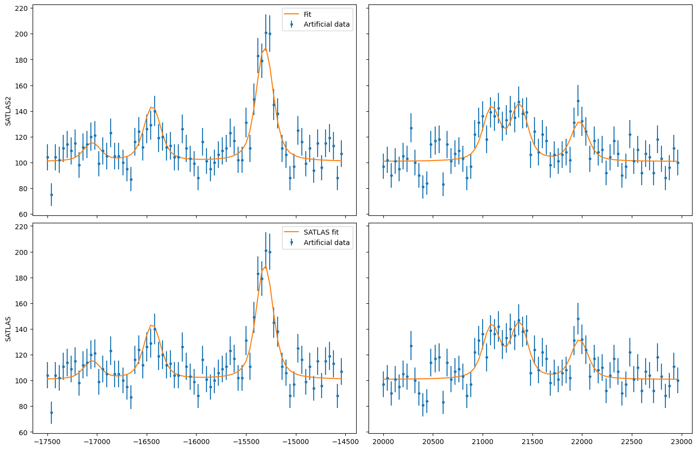
Overlapping hyperfine spectra[#](https://iks-nm.github.io/satlas2/tutorials/interface/index.html#overlapping-hyperfine-spectra "Permalink to this heading")
------------------------------------------------------------------------------------------------------------------------------------------------------------
The other most common usecase for SATLAS was analysis of spectra with an isomer present, resulting in overlapping spectra. In the SATLAS terminology, this would result in a _SumModel_ being used. In SATLAS2, a second _HFS_ is simply added to the Source. However, the interface does provide the folllowing functionality:
J = \[0.5, 1.5\]
FWHMG = 135
FWHML = 101
spin1 = 4
A1 = \[5300, 100\]
B1 = \[0, 230\]
C1 = \[0, 0\]
centroid1 = 400
bkg1 = 60
scale1 = 90
spin2 = 7
A2 = \[3300, 60\]
B2 = \[0, 270\]
C2 = \[0, 0\]
centroid2 = -100
bkg2 = 60
scale2 = 160
x = np.arange(-13000, -9000, 40)
x = np.hstack(\[x, np.arange(11000, 14000, 40)\])
rng = np.random.default\_rng(0)
# Interface models
hfs1 = satlas2.HFSModel(I=spin1,
J=J,
ABC=\[A1\[0\], A1\[1\], B1\[0\], B1\[1\], C1\[0\], C1\[1\]\],
centroid=centroid1,
fwhm=\[FWHMG, FWHML\],
scale=scale1,
background\_params=\[bkg1\],
use\_racah=True)
hfs1.set\_variation({'Cu': False})
hfs2 = satlas2.HFSModel(I=spin2,
J=J,
ABC=\[A2\[0\], A2\[1\], B2\[0\], B2\[1\], C2\[0\], C2\[1\]\],
centroid=centroid2,
fwhm=\[FWHMG, FWHML\],
scale=scale2,
background\_params=\[bkg2\],
use\_racah=True)
hfs2.set\_variation({'Cu': False})
y = satlas2.generateSpectrum(\[hfs1, hfs2, satlas2.Polynomial(\[bkg1\])\], x, rng.poisson)
hfs1.params\['centroid'\].value = centroid1 - 100
hfs2.params\['centroid'\].value = centroid2 - 100
summodel = satlas2.SumModel(\[hfs1, hfs2\], {
'values': \[bkg1, bkg2\],
'bounds': \[0\]
})
# SATLAS implementation
hfs3 = sat.HFSModel(spin1,
J, \[A1\[0\], A1\[1\], B1\[0\], B1\[1\], C1\[0\], C1\[1\]\],
centroid1-100, \[FWHMG, FWHML\],
scale=scale1,
background\_params=bkg,
use\_racah=True)
hfs4 = sat.HFSModel(spin2,
J, \[A2\[0\], A2\[1\], B2\[0\], B2\[1\], C2\[0\], C2\[1\]\],
centroid2-100, \[FWHMG, FWHML\],
scale=scale2,
background\_params=\[0\],
use\_racah=True)
hfs3.set\_variation({'Cu': False})
hfs4.set\_variation({'Background0': False, 'Cu': False})
summodel2 = hfs3 + hfs4
print('Fitting 1 dataset with chisquare (Pearson, satlas2)...')
start = time.time()
f = satlas2.chisquare\_fit(summodel, x, y, modifiedSqrt(y))
stop = time.time()
print(summodel.display\_chisquare\_fit(show\_correl=False))
dt1 = stop - start
start = time.time()
sat.chisquare\_fit(summodel2, x, y, modifiedSqrt(y))
stop = time.time()
summodel2.display\_chisquare\_fit(show\_correl=False, scaled=True)
dt2 = stop - start
print('SATLAS2: {:.3} s'.format(dt1))
print('SATLAS1: {:.3} s'.format(dt2))
Fitting 1 dataset with chisquare (Pearson, satlas2)...
\[\[Fit Statistics\]\]
\# fitting method = leastsq
\# function evals = 423
\# data points = 175
\# variables = 16
chi\-square \= 177.052463
reduced chi\-square \= 1.11353750
Akaike info crit \= 34.0405200
Bayesian info crit \= 84.6770956
\[\[Variables\]\]
Fit\_\_\_HFModel\_\_4\_\_\_centroid: 392.980617 +/- 13.2182180 (3.36%) (init \= 300)
Fit\_\_\_HFModel\_\_4\_\_\_Al: 5306.16636 +/- 9.74519323 (0.18%) (init \= 5300)
Fit\_\_\_HFModel\_\_4\_\_\_Au: 103.560669 +/- 4.03858459 (3.90%) (init \= 100)
Fit\_\_\_HFModel\_\_4\_\_\_Bl: 0 (fixed)
Fit\_\_\_HFModel\_\_4\_\_\_Bu: 195.784015 +/- 32.9150928 (16.81%) (init \= 230)
Fit\_\_\_HFModel\_\_4\_\_\_Cl: 0 (fixed)
Fit\_\_\_HFModel\_\_4\_\_\_Cu: 0 (fixed)
Fit\_\_\_HFModel\_\_4\_\_\_FWHMG: 251.277769 +/- 25.0965330 (9.99%) (init \= 135)
Fit\_\_\_HFModel\_\_4\_\_\_FWHML: 0.01000055 +/- 4.50439705 (45041.49%) (init \= 101)
Fit\_\_\_HFModel\_\_4\_\_\_scale: 79.7727405 +/- 7.53870955 (9.45%) (init \= 90)
Fit\_\_\_HFModel\_\_4\_\_\_Amp7\_2to5\_2: 0.5 (fixed)
Fit\_\_\_HFModel\_\_4\_\_\_Amp7\_2to7\_2: 0.4938272 (fixed)
Fit\_\_\_HFModel\_\_4\_\_\_Amp7\_2to9\_2: 0.3395062 (fixed)
Fit\_\_\_HFModel\_\_4\_\_\_Amp9\_2to7\_2: 0.1728395 (fixed)
Fit\_\_\_HFModel\_\_4\_\_\_Amp9\_2to9\_2: 0.4938272 (fixed)
Fit\_\_\_HFModel\_\_4\_\_\_Amp9\_2to11\_2: 1 (fixed)
Fit\_\_\_HFModel\_\_7\_\_\_centroid: \-104.843040 +/- 5.61216015 (5.35%) (init \= \-200)
Fit\_\_\_HFModel\_\_7\_\_\_Al: 3299.38314 +/- 2.54164939 (0.08%) (init \= 3300)
Fit\_\_\_HFModel\_\_7\_\_\_Au: 60.0125639 +/- 0.99398820 (1.66%) (init \= 60)
Fit\_\_\_HFModel\_\_7\_\_\_Bl: 0 (fixed)
Fit\_\_\_HFModel\_\_7\_\_\_Bu: 273.049192 +/- 15.5843734 (5.71%) (init \= 270)
Fit\_\_\_HFModel\_\_7\_\_\_Cl: 0 (fixed)
Fit\_\_\_HFModel\_\_7\_\_\_Cu: 0 (fixed)
Fit\_\_\_HFModel\_\_7\_\_\_FWHMG: 121.107402 +/- 39.0810172 (32.27%) (init \= 135)
Fit\_\_\_HFModel\_\_7\_\_\_FWHML: 112.746219 +/- 36.9166340 (32.74%) (init \= 101)
Fit\_\_\_HFModel\_\_7\_\_\_scale: 163.484079 +/- 9.34512379 (5.72%) (init \= 160)
Fit\_\_\_HFModel\_\_7\_\_\_Amp13\_2to11\_2: 0.6666667 (fixed)
Fit\_\_\_HFModel\_\_7\_\_\_Amp13\_2to13\_2: 0.5530864 (fixed)
Fit\_\_\_HFModel\_\_7\_\_\_Amp13\_2to15\_2: 0.3358025 (fixed)
Fit\_\_\_HFModel\_\_7\_\_\_Amp15\_2to13\_2: 0.2246914 (fixed)
Fit\_\_\_HFModel\_\_7\_\_\_Amp15\_2to15\_2: 0.5530864 (fixed)
Fit\_\_\_HFModel\_\_7\_\_\_Amp15\_2to17\_2: 1 (fixed)
Fit\_\_\_bkg\_\_\_value1: 60.4476367 +/- 2.36128234 (3.91%) (init \= 60)
Fit\_\_\_bkg\_\_\_value0: 61.4896354 +/- 2.12969392 (3.46%) (init \= 60)
Chisquare fitting done: 421it \[00:12, 32.65it/s\]
NDoF: 160, Chisquare: 177.29488, Reduced Chisquare: 1.108093
Akaike Information Criterium: 32.27996, Bayesian Information Criterium: 79.751749
Errors scaled with reduced chisquare.
\[\[Variables\]\]
s0\_FWHMG: 250.753540 +/- 26.0746636 (10.40%) (init \= 250.7535)
s0\_FWHML: 1.00000275 +/- 11.8677590 (1186.77%) (init \= 1.000003)
s0\_TotalFWHM: 251.288574 +/- 24.9165138 (9.92%) \== '0.5346\*s0\_FWHML+(0.2166\*s0\_FWHML\*\*2+s0\_FWHMG\*\*2)\*\*0.5'
s0\_Scale: 79.7123062 +/- 7.13677345 (8.95%) (init \= 79.71231)
s0\_Saturation: 0 (fixed)
s0\_Amp7\_2\_\_5\_2: 0.5000937 (fixed)
s0\_Amp7\_2\_\_7\_2: 0.4939217 (fixed)
s0\_Amp7\_2\_\_9\_2: 0.3396039 (fixed)
s0\_Amp9\_2\_\_7\_2: 0.172911 (fixed)
s0\_Amp9\_2\_\_9\_2: 0.4939521 (fixed)
s0\_Amp9\_2\_\_11\_2: 1 (fixed)
s0\_Al: 5306.11719 +/- 9.76080435 (0.18%) (init \= 5306.117)
s0\_Au: 103.549437 +/- 4.12089719 (3.98%) (init \= 103.5494)
s0\_Bl: 0 (fixed)
s0\_Bu: 196.011593 +/- 32.8509112 (16.76%) (init \= 196.0116)
s0\_Cl: 0 (fixed)
s0\_Cu: 0 (fixed)
s0\_Centroid: 392.909905 +/- 13.1577474 (3.35%) (init \= 392.9099)
s0\_Background0: 181.069305 +/- 1.91537125 (1.06%) (init \= 181.0693)
s0\_N: 0 (fixed)
s1\_FWHMG: 121.817424 +/- 39.1318124 (32.12%) (init \= 121.8174)
s1\_FWHML: 112.056361 +/- 37.1055724 (33.11%) (init \= 112.0564)
s1\_TotalFWHM: 192.416653 +/- 15.7236790 (8.17%) \== '0.5346\*s1\_FWHML+(0.2166\*s1\_FWHML\*\*2+s1\_FWHMG\*\*2)\*\*0.5'
s1\_Scale: 163.317972 +/- 9.22593437 (5.65%) (init \= 163.318)
s1\_Saturation: 0 (fixed)
s1\_Amp13\_2\_\_11\_2: 0.666746 (fixed)
s1\_Amp13\_2\_\_13\_2: 0.5531882 (fixed)
s1\_Amp13\_2\_\_15\_2: 0.3359059 (fixed)
s1\_Amp15\_2\_\_13\_2: 0.2247785 (fixed)
s1\_Amp15\_2\_\_15\_2: 0.55321 (fixed)
s1\_Amp15\_2\_\_17\_2: 1 (fixed)
s1\_Al: 3299.37436 +/- 2.48138492 (0.08%) (init \= 3299.374)
s1\_Au: 60.0050608 +/- 0.98060493 (1.63%) (init \= 60.00506)
s1\_Bl: 0 (fixed)
s1\_Bu: 273.161795 +/- 15.4999419 (5.67%) (init \= 273.1618)
s1\_Cl: 0 (fixed)
s1\_Cu: 0 (fixed)
s1\_Centroid: \-104.833860 +/- 5.57438226 (5.32%) (init \= \-104.8339)
s1\_Background0: 0 (fixed)
s1\_N: 0 (fixed)
SATLAS2: 0.226 s
SATLAS1: 12.9 s
The difference in coding implementation is a result of the interface automatically implementing a PiecewiseConstant background, where the background is a constant for different regions in _x_\-space. Notice here that the speedup due using the SATLAS2 implementation has risen from a factor 20 for a single spectrum to almost a factor 60.
left\_x = x\[x<0\]
right\_x = x\[x>0\]
left\_y = y\[x<0\]
right\_y = y\[x>0\]
fig = plt.figure(constrained\_layout=True, figsize=(14, 9))
gs = gridspec.GridSpec(nrows=2, ncols=2, figure=fig)
ax11 = fig.add\_subplot(gs\[0, 0\])
ax11.label\_outer()
ax12 = fig.add\_subplot(gs\[0, 1\], sharey=ax11)
ax12.label\_outer()
ax21 = fig.add\_subplot(gs\[1, 0\], sharex=ax11)
ax21.label\_outer()
ax22 = fig.add\_subplot(gs\[1, 1\], sharex=ax12, sharey=ax21)
ax22.label\_outer()
ax11.errorbar(left\_x, left\_y, modifiedSqrt(left\_y), fmt='.', label='Artificial data')
ax11.plot(left\_x, hfs1(left\_x), '-', label='SATLAS2 fit model 1')
ax11.plot(left\_x, hfs2(left\_x), '-', label='SATLAS2 fit model 2')
ax11.plot(left\_x, summodel(left\_x), '-', label='Sum of models')
ax12.errorbar(right\_x, right\_y, modifiedSqrt(right\_y), fmt='.', label='Artificial data')
ax12.plot(right\_x, hfs1(right\_x), '-', label='SATLAS2 fit model 1')
ax12.plot(right\_x, hfs2(right\_x), '-', label='SATLAS2 fit model 2')
ax12.plot(right\_x, summodel(right\_x), '-', label='Sum of models')
ax11.legend()
ax21.errorbar(left\_x, left\_y, modifiedSqrt(left\_y), fmt='.', label='Artificial data')
ax21.plot(left\_x, hfs3(left\_x), '-', label='SATLAS fit model 1')
ax21.plot(left\_x, hfs4(left\_x), '-', label='SATLAS fit model 2')
ax21.plot(left\_x, summodel2(left\_x), '-', label='Sum of models')
ax22.errorbar(right\_x, right\_y, modifiedSqrt(right\_y), fmt='.', label='Artificial data')
ax22.plot(right\_x, hfs3(right\_x), '-', label='SATLAS fit model 1')
ax22.plot(right\_x, hfs4(right\_x), '-', label='SATLAS fit model 2')
ax22.plot(right\_x, summodel2(right\_x), '-', label='Sum of models')
ax21.legend()
ax11.set\_ylabel('SATLAS2')
ax21.set\_ylabel('SATLAS')
plt.show()
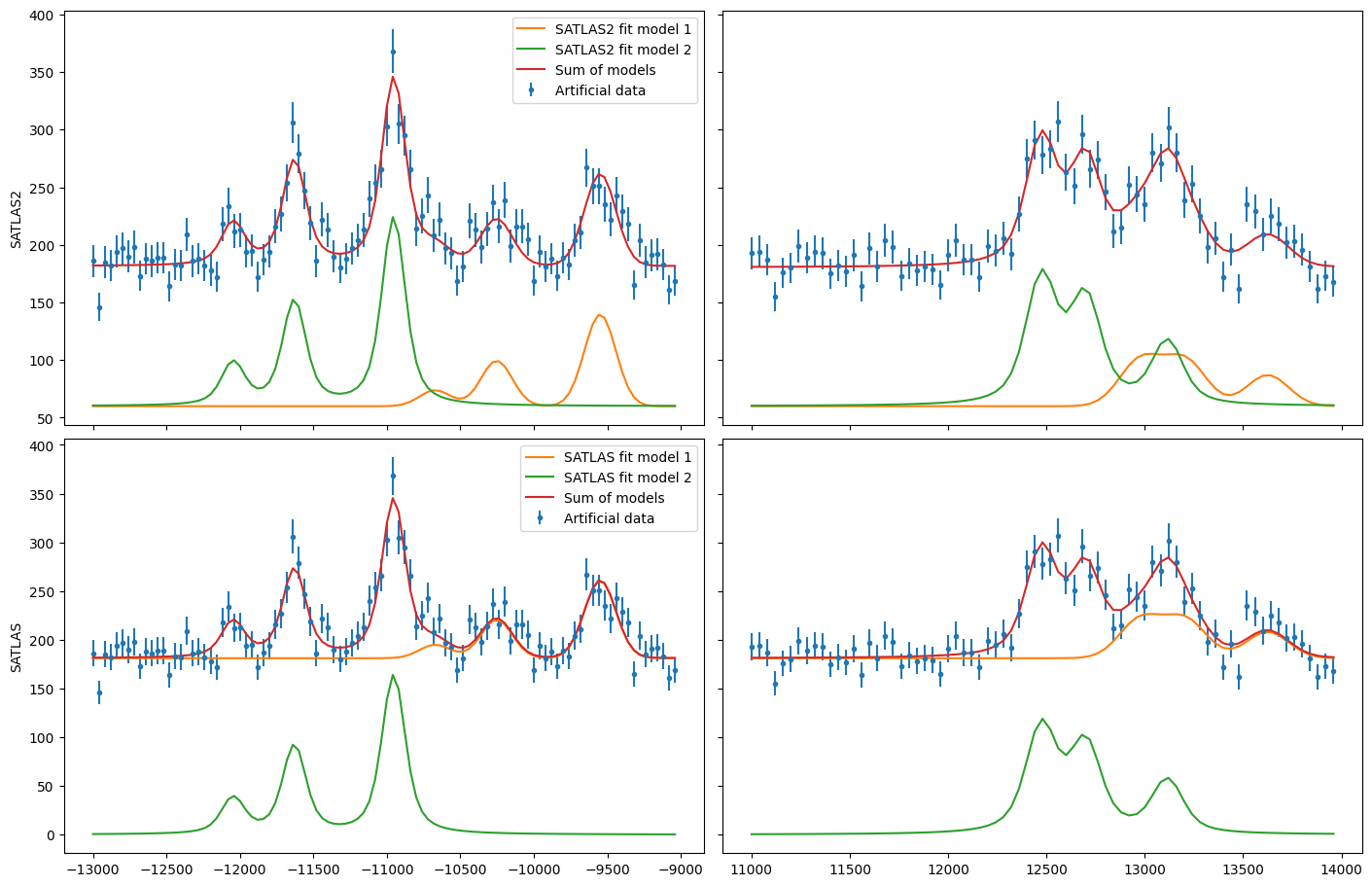
Different background for multiplets[#](https://iks-nm.github.io/satlas2/tutorials/interface/index.html#different-background-for-multiplets "Permalink to this heading")
------------------------------------------------------------------------------------------------------------------------------------------------------------------------
To demonstrate the convenience of the PiecewiseConstant background, the same results are coded with SATLAS, where the use of LinkedModel is required. Note that here, the interface is _not_ used.
J = \[0.5, 1.5\]
FWHMG = 135
FWHML = 101
spin1 = 4
A1 = \[5300, 100\]
B1 = \[0, 230\]
C1 = \[0, 0\]
centroid1 = 400
bkg1 = 90
scale1 = 90
x = np.arange(-13000, -9000, 40)
x = np.hstack(\[x, np.arange(11000, 14000, 40)\])
hfs = satlas2.HFS(spin1,
J=J,
A=\[A1\[0\], A1\[1\]\],
B=\[B1\[0\], B1\[1\]\],
C=\[C1\[0\], C1\[1\]\],
df=centroid1,
fwhmg=FWHMG,
fwhml=FWHML,
scale=scale1,
racah=True
)
hfs.params\['Cu'\].vary = False
bkg = satlas2.PiecewiseConstant(\[bkg1, bkg2\], \[0\])
y = satlas2.generateSpectrum(\[hfs1, bkg\], x, rng.poisson)
s = satlas2.Source(x, y, yerr=modifiedSqrt, name='Artificial')
s.addModel(hfs)
s.addModel(bkg)
f = satlas2.Fitter()
f.addSource(s)
hfs2 = sat.HFSModel(spin1,
J, \[A1\[0\], A1\[1\], B1\[0\], B1\[1\], C1\[0\], C1\[1\]\],
centroid - 100, \[FWHMG, FWHML\],
scale=scale1,
background\_params=\[bkg1\],
use\_racah=True)
hfs3 = sat.HFSModel(spin1,
J, \[A1\[0\], A1\[1\], B1\[0\], B1\[1\], C1\[0\], C1\[1\]\],
centroid - 100, \[FWHMG, FWHML\],
scale=scale1,
background\_params=\[bkg1\],
use\_racah=True)
hfs2.set\_variation({'Cu': False})
hfs3.set\_variation({'Cu': False})
linkedmodel = sat.LinkedModel(\[hfs2, hfs3\])
linkedmodel.shared = \['Al', 'Au', 'Bl', 'Bu', 'Centroid'\]
linked\_x = \[x\[x<0\], x\[x>0\]\]
linked\_y = \[y\[x<0\], y\[x>0\]\]
print('Fitting 1 dataset with chisquare (Pearson, satlas2)...')
start = time.time()
f.fit()
stop = time.time()
print(f.reportFit())
dt1 = stop - start
start = time.time()
sat.chisquare\_spectroscopic\_fit(linkedmodel, linked\_x, linked\_y, func=modifiedSqrt)
stop = time.time()
linkedmodel.display\_chisquare\_fit(show\_correl=False, scaled=True)
dt2 = stop - start
print('SATLAS2: {:.3} s'.format(dt1))
print('SATLAS1: {:.3} s'.format(dt2))
Fitting 1 dataset with chisquare (Pearson, satlas2)...
\[\[Fit Statistics\]\]
\# fitting method = leastsq
\# function evals = 202
\# data points = 175
\# variables = 9
chi\-square \= 162.334878
reduced chi\-square \= 0.97792095
Akaike info crit \= 4.85319079
Bayesian info crit \= 33.3362646
\[\[Variables\]\]
Artificial\_\_\_HFS\_\_\_centroid: 379.439738 +/- 11.8479412 (3.12%) (init \= 400)
Artificial\_\_\_HFS\_\_\_Al: 5300.53685 +/- 8.60042067 (0.16%) (init \= 5300)
Artificial\_\_\_HFS\_\_\_Au: 100.910641 +/- 3.43441833 (3.40%) (init \= 100)
Artificial\_\_\_HFS\_\_\_Bl: 0 (fixed)
Artificial\_\_\_HFS\_\_\_Bu: 167.829114 +/- 27.5840684 (16.44%) (init \= 230)
Artificial\_\_\_HFS\_\_\_Cl: 0 (fixed)
Artificial\_\_\_HFS\_\_\_Cu: 0 (fixed)
Artificial\_\_\_HFS\_\_\_FWHMG: 257.963959 +/- 23.7214758 (9.20%) (init \= 135)
Artificial\_\_\_HFS\_\_\_FWHML: 0.01005831 +/- 46.0743167 (458072.02%) (init \= 101)
Artificial\_\_\_HFS\_\_\_scale: 73.5969741 +/- 6.04333358 (8.21%) (init \= 90)
Artificial\_\_\_HFS\_\_\_Amp7\_2to5\_2: 0.5 (fixed)
Artificial\_\_\_HFS\_\_\_Amp7\_2to7\_2: 0.4938272 (fixed)
Artificial\_\_\_HFS\_\_\_Amp7\_2to9\_2: 0.3395062 (fixed)
Artificial\_\_\_HFS\_\_\_Amp9\_2to7\_2: 0.1728395 (fixed)
Artificial\_\_\_HFS\_\_\_Amp9\_2to9\_2: 0.4938272 (fixed)
Artificial\_\_\_HFS\_\_\_Amp9\_2to11\_2: 1 (fixed)
Artificial\_\_\_PiecewiseConstant\_\_\_value1: 122.518511 +/- 1.44251185 (1.18%) (init \= 60)
Artificial\_\_\_PiecewiseConstant\_\_\_value0: 151.305847 +/- 1.37967336 (0.91%) (init \= 90)
Chisquare fitting done: 619it \[00:19, 31.30it/s\]
NDoF: 163, Chisquare: 158.72971, Reduced Chisquare: 0.97380192
Akaike Information Criterium: 6.9229505, Bayesian Information Criterium: 44.900382
Errors scaled with reduced chisquare.
\[\[Variables\]\]
s0\_FWHMG: 287.317538 (init \= 287.3175)
s0\_FWHML: 1.00000004 (init \= 1)
s0\_TotalFWHM: 287.852515 \== '0.5346\*s0\_FWHML+(0.2166\*s0\_FWHML\*\*2+s0\_FWHMG\*\*2)\*\*0.5'
s0\_Scale: 72.0818067 (init \= 72.08181)
s0\_Saturation: 0 (fixed)
s0\_Amp7\_2\_\_5\_2: 0.5000937 (fixed)
s0\_Amp7\_2\_\_7\_2: 0.4939217 (fixed)
s0\_Amp7\_2\_\_9\_2: 0.3396039 (fixed)
s0\_Amp9\_2\_\_7\_2: 0.172911 (fixed)
s0\_Amp9\_2\_\_9\_2: 0.4939521 (fixed)
s0\_Amp9\_2\_\_11\_2: 1 (fixed)
s0\_Al: 5300.79815 (init \= 5300.798)
s0\_Au: 101.129022 (init \= 101.129)
s0\_Bl: 0 (fixed)
s0\_Bu: 171.971287 (init \= 171.9713)
s0\_Cl: 0 (fixed)
s0\_Cu: 0 (fixed)
s0\_Centroid: 377.508491 (init \= 377.5085)
s0\_Background0: 150.539789 (init \= 150.5398)
s0\_N: 0 (fixed)
s1\_FWHMG: 208.133894 (init \= 208.1339)
s1\_FWHML: 1.00001971 (init \= 1.00002)
s1\_TotalFWHM: 208.669025 \== '0.5346\*s1\_FWHML+(0.2166\*s1\_FWHML\*\*2+s1\_FWHMG\*\*2)\*\*0.5'
s1\_Scale: 82.8509918 (init \= 82.85099)
s1\_Saturation: 0 (fixed)
s1\_Amp7\_2\_\_5\_2: 0.5000937 (fixed)
s1\_Amp7\_2\_\_7\_2: 0.4939217 (fixed)
s1\_Amp7\_2\_\_9\_2: 0.3396039 (fixed)
s1\_Amp9\_2\_\_7\_2: 0.172911 (fixed)
s1\_Amp9\_2\_\_9\_2: 0.4939521 (fixed)
s1\_Amp9\_2\_\_11\_2: 1 (fixed)
s1\_Al: 5300.79815 \== 's0\_Al'
s1\_Au: 101.129022 \== 's0\_Au'
s1\_Bl: 0.00000000 \== 's0\_Bl'
s1\_Bu: 171.971287 \== 's0\_Bu'
s1\_Cl: 0 (fixed)
s1\_Cu: 0 (fixed)
s1\_Centroid: 377.508491 \== 's0\_Centroid'
s1\_Background0: 123.248661 (init \= 123.2487)
s1\_N: 0 (fixed)
SATLAS2: 0.107 s
SATLAS1: 19.8 s
fig = plt.figure(constrained\_layout=True, figsize=(14, 9))
gs = gridspec.GridSpec(nrows=2, ncols=2, figure=fig)
ax11 = fig.add\_subplot(gs\[0, 0\])
ax11.label\_outer()
ax12 = fig.add\_subplot(gs\[0, 1\], sharey=ax11)
ax12.label\_outer()
ax21 = fig.add\_subplot(gs\[1, 0\], sharex=ax11)
ax21.label\_outer()
ax22 = fig.add\_subplot(gs\[1, 1\], sharex=ax12, sharey=ax21)
ax22.label\_outer()
ax11.errorbar(linked\_x\[0\], linked\_y\[0\], modifiedSqrt(linked\_y\[0\]), fmt='.', label='Artificial data')
ax11.plot(linked\_x\[0\], s.evaluate(linked\_x\[0\]), '-', label='Fit')
ax12.errorbar(linked\_x\[1\], linked\_y\[1\], modifiedSqrt(linked\_y\[1\]), fmt='.', label='Artificial data')
ax12.plot(linked\_x\[1\], s.evaluate(linked\_x\[1\]), '-', label='SATLAS2 fit model 1')
ax11.legend()
ax21.errorbar(linked\_x\[0\], linked\_y\[0\], modifiedSqrt(linked\_y\[0\]), fmt='.', label='Artificial data')
ax21.plot(linked\_x\[0\], linkedmodel.models\[0\](linked\_x\[0\]), '-', label='Fit')
ax22.errorbar(linked\_x\[1\], linked\_y\[1\], modifiedSqrt(linked\_y\[1\]), fmt='.', label='Artificial data')
ax22.plot(linked\_x\[1\], linkedmodel.models\[1\](linked\_x\[1\]), '-', label='Fit')
ax21.legend()
ax11.set\_ylabel('SATLAS2')
ax21.set\_ylabel('SATLAS')
plt.show()
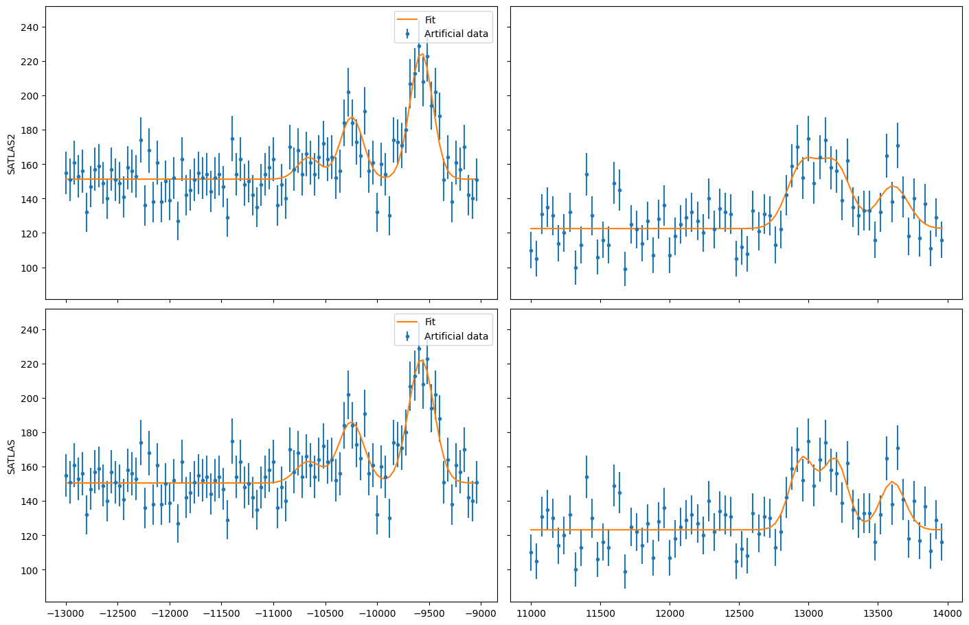
Contents
---
# Unknown
Extracting dataframes ===================== The results of a fit can be extracted from the Fitter object in the format of a Pandas DataFrame. Aside from the results themselves, the additional statistics from the fitting can also be extracted in a separate DataFrame. This will be demonstrated by fitting multiple spectra of a Voigt peak on top of an exponential background: .. code:: ipython3 import sys sys.path.insert(0, '..\\src') from io import BytesIO import matplotlib.pyplot as plt import numpy as np import pandas as pd import satlas2 def modifiedSqrt(input): output = np.sqrt(input) output\[input <= 0\] = 1 return output def createModels(backg, lamda, loc, fwhmg, fwhml, amp): bkg = satlas2.ExponentialDecay(backg, lamda, name='Background') peak = satlas2.Voigt(amp, loc, fwhmg, fwhml, name='Signal') return peak, bkg Defining the parameters and preparing the needed arrays for saving the results: .. code:: ipython3 loc = 500 fwhmg = 150 fwhml = 150 amp = 200 bkg1 = 1000 bkg2 = 500 bkg3 = 700 lamda = 500 rng = np.random.default\_rng(0) x = np.linspace(0, 1000, 250) bkgs = \[bkg1, bkg2, bkg3\] names = \['Scan1', 'Scan2', 'Scan3'\] metadata = \[\] results = \[\] imgdatas = \[\] In a loop, generate three different datasets and fit them separately. The plots are saved to a BytesIO object for saving to an Excel spreadsheet later. .. code:: ipython3 for bkg, name in zip(bkgs, names): peakm, bkgm = createModels(bkg, lamda, loc, fwhmg, fwhml, amp) y = satlas2.generateSpectrum(\[peakm, bkgm\], x, rng.poisson) fig = plt.figure() ax = fig.add\_axes(\[0.1, 0.1, 0.8, 0.8\]) ax.plot(x, y, 'o', label='Data') ax.set\_xlabel('x') ax.set\_ylabel('y') datasource = satlas2.Source(x, y, yerr=modifiedSqrt, name=name) datasource.addModel(peakm) datasource.addModel(bkgm) f = satlas2.Fitter() f.addSource(datasource) f.fit() ax.plot(datasource.x, datasource.f(), label='Fit') ax.set\_title(name) ax.legend(loc=0) metadata.append(f.createMetadataDataframe()) results.append(f.createResultDataframe()) imgdata = BytesIO() fig.savefig(imgdata, format='png') imgdatas.append(imgdata) metadata = pd.concat(metadata) results = pd.concat(results) The \*metadata\* and \*results\* DataFrames now contain the fitting statistics and parameter results of all three fits respectively. As an example of how this can be processed later, the DataFrames along with the plots will be saved to an Excel sheet in the following section: .. code:: ipython3 filename = 'test.xlsx' figwidth = 10 # Standard figure size is about 10 cells with pd.ExcelWriter(filename, engine='xlsxwriter') as writer: metadata.to\_excel(writer, sheet\_name='Metadata', index=False) results.to\_excel(writer, sheet\_name='Results', index=False) workbook = writer.book red\_format = workbook.add\_format({ 'bg\_color': '#FFC7CE', 'font\_color': '#9C0006' }) green\_format = workbook.add\_format({ 'bg\_color': '#C6EFCE', 'font\_color': '#006100' }) yellow\_format = workbook.add\_format({ 'bg\_color': '#FFEB9C', 'font\_color': '#9C5700' }) metadatasheet = workbook.get\_worksheet\_by\_name('Metadata') resultssheet = workbook.get\_worksheet\_by\_name('Results') figuressheet = workbook.add\_worksheet('Figures') for i, im in enumerate(imgdatas): im.seek(0) figuressheet.insert\_image(0, 0 + i \* 10, "", {'image\_data': im}) # Add conditional formatting to illustrate reduced chisquares that # are above the 1-sigma estimate for the reduced chisquare metadatasheet.conditional\_format( 'H2:H99', { 'type': 'cell', 'criteria': 'not between', 'minimum': '=1-SQRT(2/(E2:E99-F2:F99))', 'maximum': '=1+SQRT(2/(E2:E99-F2:F99))', 'format': yellow\_format }) metadatasheet.conditional\_format( 'H2:H99', { 'type': 'cell', 'criteria': 'between', 'minimum': '=1-SQRT(2/(E2:E99-F2:F99))', 'maximum': '=1+SQRT(2/(E2:E99-F2:F99))', 'format': green\_format }) try: metadatasheet.autofit() resultssheet.autofit() except: pass This results in an Excel sheet with the first sheet looking like this: .. image:: sheet1.png The second sheet contains the parameter results: .. image:: sheet2.png And the third sheet contains figures of the three datasets: .. image:: sheet3.png
---
# Unknown
Making a model ============== As illustrated in the architecture page, SATLAS2 is built on the concept of a Fitter object, to which Source objects are assigned. These Source objects contain both experimental data, but are also assigned one or more Models, which should be fitted to the data. The base aspect of these Models is that two things should be implemented: a \*params\* attribute which is a dictionary containing all the Parameters that the Model needs, and a method \*f(x)\*, where the response for the given \*x\* values is returned. It is recommended that the first line of the method is \*x = self.transform(x)\* in order to correctly handle any transformation functions that are required. In this tutorial, a new Model will be created to model a sine wave with exponential damping called \*ExpSine\*, just as an example. In the preamble, we just import all the libraries that we will need. .. code:: ipython3 import sys sys.path.insert(0, '..\\src') import matplotlib.pyplot as plt import numpy as np import satlas2 Subclassing Model ----------------- The new class will be a subclass of the SATLAS2 Model class, and it will contain SATLAS2 Parameters in its \*params\* dictionary. .. code:: ipython3 class ExpSine(satlas2.Model): def \_\_init\_\_(self, A, lamda, omega, name='ExpSine', prefunc=None): super().\_\_init\_\_(name, prefunc=prefunc) self.params={ 'amplitude': satlas2.Parameter(value=A,min=0,max=np.inf,vary=True), 'lambda': satlas2.Parameter(value=lamda, min=0, max=np.inf, vary=True), 'omega': satlas2.Parameter(value=omega, min=0, max=np.inf, vary=True) } def f(self, x): x = self.transform(x) a = self.params\['amplitude'\].value l = self.params\['lambda'\].value o = self.params\['omega'\].value return a\*np.exp(-l\*x)\*np.sin(o\*x) This defines a sine wave of angular frequency ω with an exponential decay with decay constant λ. Note that, in the parameter name in \*\*init\*\*, \*lamda\* is used instead of \*lambda\* since the last one is a keyword in Python. With this new Model, plotting is done in the following way: .. code:: ipython3 amplitude = 7 lamda = 1.5 omega = 4 model = ExpSine(amplitude, lamda, omega, name='MyModel') x = np.linspace(0, 4, 100) y = model.f(x) fig = plt.figure() ax = fig.add\_axes(\[0.1, 0.1, 0.8, 0.8\]) ax.plot(x, y) ax.set\_xlabel('x') ax.set\_ylabel('y') ax.set\_title('My ExpSine Model') model.params .. parsed-literal:: {'amplitude': 7+/-0 (inf max, 0 min, vary=True, correl={}), 'lambda': 1.5+/-0 (inf max, 0 min, vary=True, correl={}), 'omega': 4+/-0 (inf max, 0 min, vary=True, correl={})} .. image:: output\_5\_1.png Data generation and fitting --------------------------- The model defined above is fully compatible with all SATLAS2 code and can be used to fit data. To illustrate this feature, a dataset needs to be generated. For this, SATLAS2 contains a convenience function. The standard argument generates a dataset that assumes the model supplies the mean value of a Poisson distribution, which is useful for simulation of laser spectroscopy spectra. However, the generator can be modified, allowing generic Gaussian data to be generated as well: .. code:: ipython3 data\_x = np.linspace(0, 4, 20) noise = 1.5 generator = lambda x: np.random.default\_rng(0).normal(x, noise) data\_y = satlas2.generateSpectrum(model, data\_x, generator=generator) yerr = np.ones(data\_y.shape)\*noise fig = plt.figure() ax = fig.add\_axes(\[0.1, 0.1, 0.8, 0.8\]) ax.errorbar(data\_x, data\_y, yerr=yerr, fmt='o', label='Data') ax.plot(x, y, label='Initial guess') ax.set\_xlabel('x') ax.set\_ylabel('y') ax.legend(loc=0) .. image:: output\_7\_0.png We assign this data to a Source, add the ExpSine model to this Source, and pass it to a Fitter to fit this. Since this requires a normal chisquare fit, no extra arguments are required for the fit. .. code:: ipython3 datasource = satlas2.Source(data\_x, data\_y, yerr=yerr, name='Datafile1') datasource.addModel(model) f = satlas2.Fitter() f.addSource(datasource) f.fit() print(f.reportFit()) fig = plt.figure() ax = fig.add\_axes(\[0.1, 0.1, 0.8, 0.8\]) ax.errorbar(data\_x, data\_y, yerr=yerr, fmt='o', label='Data') ax.plot(x, y, label='Initial guess') ax.plot(x, model.f(x), label='Fit') ax.set\_xlabel('x') ax.set\_ylabel('y') ax.legend(loc=0) .. parsed-literal:: \[\[Fit Statistics\]\] # fitting method = leastsq # function evals = 93 # data points = 20 # variables = 3 chi-square = 14.1735643 reduced chi-square = 0.83373907 Akaike info crit = -0.88707432 Bayesian info crit = 2.10012250 \[\[Variables\]\] Datafile1\_\_\_MyModel\_\_\_amplitude: 9.03884096 +/- 4.31842559 (47.78%) (init = 7) Datafile1\_\_\_MyModel\_\_\_lambda: 2.15722712 +/- 1.22083220 (56.59%) (init = 1.5) Datafile1\_\_\_MyModel\_\_\_omega: 4.22415871 +/- 0.68336353 (16.18%) (init = 4) .. image:: output\_9\_1.png
---
# Unknown
Different \`\`emcee\`\` moves ========================= The \`\`emcee\`\` library that is used for the random walk exploration of the parameter space has some options that are exposed in the SATLAS2 interface. One interesting option is the ability to change the algorithms used to propose moves. The \`\`emcee\`\` documentation contains a tutorial on how and why different moves can be used \`here \`\_\_. The exploration of the parameter space for hyperfine spectra does benefit from this option. The difference between the standard stretch move and the proposed mix of differential evolution move and snooker move will be explored. .. code:: ipython3 import sys import time import emcee import matplotlib.gridspec as gridspec import matplotlib.pyplot as plt import numpy as np sys.path.insert(0, '..\\..\\..\\src') import satlas2 def modifiedSqrt(input): output = np.sqrt(input) output\[input <= 0\] = 1 return output Data generation --------------- The convenience function included in SATLAS2 is used to generate a Poisson distributed spectrum. .. code:: ipython3 A = \[50, 250\] B = \[10, 5\] C = \[0, 0\] I = 1.0 J = \[1.0, 1.0\] df = 0 fwhmg = 50 fwhml = 50 scale = 200 bkg = 50 hfs = satlas2.HFS(I, J, A=A, B=B, C=C, df=df, fwhmg=fwhmg, fwhml=fwhml, scale=scale) bkg = satlas2.Polynomial(\[bkg\]) x = np.linspace(-700, 600, 1000) data\_x = np.arange(x.min(), x.max(), 15) data\_y = satlas2.generateSpectrum(\[hfs, bkg\], data\_x) plt.plot(data\_x, data\_y, drawstyle='steps-mid') plt.plot(x, hfs.f(x)+bkg.f(x)) f = satlas2.Fitter() datasource = satlas2.Source(data\_x, data\_y, yerr=modifiedSqrt, name='Artificial') datasource.addModel(hfs) datasource.addModel(bkg) f.addSource(datasource) f.fit() print(f.reportFit()) .. parsed-literal:: \[\[Fit Statistics\]\] # fitting method = leastsq # function evals = 91 # data points = 87 # variables = 9 chi-square = 72.8990076 reduced chi-square = 0.93460266 Akaike info crit = 2.61552097 Bayesian info crit = 24.8086940 \[\[Variables\]\] Artificial\_\_\_HFS\_\_\_centroid: -0.37055045 +/- 1.42164523 (383.66%) (init = 0) Artificial\_\_\_HFS\_\_\_Al: 51.4477619 +/- 1.39705770 (2.72%) (init = 50) Artificial\_\_\_HFS\_\_\_Au: 251.236334 +/- 1.65652941 (0.66%) (init = 250) Artificial\_\_\_HFS\_\_\_Bl: 12.5419832 +/- 2.59229524 (20.67%) (init = 10) Artificial\_\_\_HFS\_\_\_Bu: 4.34080560 +/- 1.74164467 (40.12%) (init = 5) Artificial\_\_\_HFS\_\_\_Cl: 0 (fixed) Artificial\_\_\_HFS\_\_\_Cu: 0 (fixed) Artificial\_\_\_HFS\_\_\_FWHMG: 56.0066443 +/- 10.2656213 (18.33%) (init = 50) Artificial\_\_\_HFS\_\_\_FWHML: 42.4534449 +/- 11.2048829 (26.39%) (init = 50) Artificial\_\_\_HFS\_\_\_scale: 205.225337 +/- 7.32534024 (3.57%) (init = 200) Artificial\_\_\_HFS\_\_\_Amp0to1: 0.2666667 (fixed) Artificial\_\_\_HFS\_\_\_Amp1to0: 0.2666667 (fixed) Artificial\_\_\_HFS\_\_\_Amp1to1: 0.2 (fixed) Artificial\_\_\_HFS\_\_\_Amp1to2: 0.3333333 (fixed) Artificial\_\_\_HFS\_\_\_Amp2to1: 0.3333333 (fixed) Artificial\_\_\_HFS\_\_\_Amp2to2: 1 (fixed) Artificial\_\_\_Polynomial\_\_\_p0: 48.4270596 +/- 1.97001650 (4.07%) (init = 50) .. image:: output\_3\_2.png Standard \`\`emcee\`\` move ----------------------- The normal move used by \`\`emcee\`\` is called the StretchMove, and is used by not specifying any specific moves at all .. code:: ipython3 stretchfile = 'stretchmove.h5' f.fit(method='emcee', filename=stretchfile) .. parsed-literal:: 100%|████████████| 1000/1000 \[00:28<00:00, 35.70it/s\] The chain is shorter than 50 times the integrated autocorrelation time for 9 parameter(s). Use this estimate with caution and run a longer chain! N/50 = 20; tau: \[52.18497247 57.73151625 50.61482182 58.94721213 55.18218592 53.97033804 51.2988931 56.19765179 49.45745584\] The warning here shows that, in order to get good estimates, more samples are recommended. For more information, see the \`\`emcee\`\` documentation. However, the important detail here is the list of autocorrelation times that is estimated here, which is about 50-60 steps. .. code:: ipython3 fig, axes = satlas2.generateWalkPlot(stretchfile) fig.set\_size\_inches(6, 10) .. image:: output\_7\_1.png Here, the burn-in is quite long for several parameters. If possible, avoiding long burn-ins is very useful to increase useful computation time. Using differential evolution moves ---------------------------------- Starting from version 3, \`\`emcee\`\` has a Moves interface where the proposal for the random walk can be changed. In addition to specifying another algorithm, a selection of moves can be given along with a float that represents the chance the algorithm is selected. Giving an ensemble of move proposals in this way can improve overall performance. As illustrated in the linked documentation, a combination of DEMove and DESnookerMove can perform better in highly dimensional or lightly multimodal distributions. Both of these descriptions can be well applied to the fitting of hyperfine spectra. .. code:: ipython3 combinationfile = 'combination.h5' f.revertFit() f.fit(method='emcee', filename=combinationfile, sampler\_kwargs={'moves': \[ (emcee.moves.DEMove(), 0.8), (emcee.moves.DESnookerMove(), 0.2) \]}) .. parsed-literal:: 100%|████████████| 1000/1000 \[00:28<00:00, 35.65it/s\] The chain is shorter than 50 times the integrated autocorrelation time for 9 parameter(s). Use this estimate with caution and run a longer chain! N/50 = 20; tau: \[25.79202768 28.04787132 31.15895649 27.02757601 27.06688899 32.62843194 33.30301554 29.44226374 30.75024705\] As with the previous case, the recommendation is that a longer chain is used. However, the autocorrelation time is much shorter, 20-30 steps instead of the previous 50-60 steps. This corresponds to a walk that shows a much lower burn-in time. .. code:: ipython3 fig, axes = satlas2.generateWalkPlot(combinationfile) fig.set\_size\_inches(6, 10) .. image:: output\_12\_1.png This is clearly reflected in the resulting walk. Experimentation with the exact mixture of Moves can result in even better performance. Since SATLAS2 relies on the interface provided by emcee, any future Moves that are introduced can automatically be used in SATLAS2 for sampling.
---
# Unknown
Benchmark of SATLAS2 speed ========================== The simultaneous fit of sets of data is shown in this notebook. The data generation code can be replaced by code that reads in datafiles, so this script can serve as the basis for your own analysis. The fitting is compared to the simulatenous fit in the first version of satlas. First, start with an import of all the relevant libraries: .. code:: ipython3 import sys import time import matplotlib.gridspec as gridspec import matplotlib.pyplot as plt import numpy as np sys.path.insert(0, '..\\src') import satlas2 import satlas as sat Define a modified root function to handle uncertainties of 0 counts in a Poisson statistic .. code:: ipython3 def modifiedSqrt(input): output = np.sqrt(input) output\[input <= 0\] = 1 return output Define all the parameters and, in a for-loop, define the HFS and background models to generate the data from. The fitting already occurs inside the for loop, so the performance can be seen as a function of the number of datasets that are being analysed. .. code:: ipython3 spin = 3.5 J = \[0.5, 1.5\] A = \[9600, 175\] B = \[0, 315\] C = \[0, 0\] FWHMG = 135 FWHML = 101 centroid = 480 bkg = 10 scale = 90 x = np.arange(-17500, -14500, 40) x = np.hstack(\[x, np.arange(20000, 23000, 40)\]) times = \[\] times\_1 = \[\] rng = np.random.default\_rng(0) for j in range(1, 11): f = satlas2.Fitter() models = \[\] X = \[\] Y = \[\] for i in range(j): hfs = satlas2.HFS(spin, J, A=A, B=B, C=C, scale=scale, df=centroid, name='HFS1', racah=True, fwhmg=135, fwhml=100) bkgm = satlas2.Polynomial(\[bkg\], name='bkg1') y = satlas2.generateSpectrum(\[hfs, bkgm\], x, rng.poisson) hfs.params\['centroid'\].value = centroid - 100 X.append(x) Y.append(y) hfs1 = sat.HFSModel(spin, J, \[A\[0\], A\[1\], B\[0\], B\[1\], C\[0\], C\[1\]\], centroid - 100, \[FWHMG, FWHML\], scale=scale, background\_params=\[bkg\], use\_racah=True) models.append(hfs1) datasource = satlas2.Source(x, y, yerr=modifiedSqrt, name='Scan{}'.format(i + 1)) datasource.addModel(hfs) datasource.addModel(bkgm) f.addSource(datasource) share = \['Al', 'Au', 'Bl', 'centroid', 'FWHMG', 'FWHML'\] m = sat.LinkedModel(models) m.shared = share f.shareModelParams(share) print('Fitting {} datasets with chisquare (Pearson, satlas2)...'.format(j)) start = time.time() f.fit() stop = time.time() dt = stop - start print('{:.3} s, {:.0f} function evaluations'.format(dt, f.result.nfev)) times.append(dt) print('Fitting {} datasets with chisquare (Pearson, satlas1)...'.format(j)) start = time.time() sat.chisquare\_spectroscopic\_fit(m, X, Y) stop = time.time() dt = stop - start times\_1.append(dt) fig = plt.figure() ax = fig.add\_axes(\[0.1, 0.1, 0.8, 0.8\]) ax.plot(range(1, len(times) + 1), times, '-o', label='satlas2') ax.plot(range(1, len(times\_1) + 1), times\_1, '-o', label='satlas1') ax.set\_xlabel('Number of datasets') ax.set\_ylabel('Fitting time in seconds') ax.set\_yscale('log') ax.legend(loc=0) times, times\_1 = np.array(times), np.array(times\_1) fig = plt.figure() ax = fig.add\_axes(\[0.1, 0.1, 0.8, 0.8\]) ax.plot(range(1, len(times) + 1), times\_1/times, '-o') ax.set\_xlabel('Number of datasets') ax.set\_ylabel('Speedup factor by using satlas2') .. parsed-literal:: Fitting 1 datasets with chisquare (Pearson, satlas2)... 0.041 s, 73 function evaluations Fitting 1 datasets with chisquare (Pearson, satlas1)... Chisquare fitting done: 98it \[00:00, 100.10it/s\] Fitting 2 datasets with chisquare (Pearson, satlas2)... 0.102 s, 110 function evaluations Fitting 2 datasets with chisquare (Pearson, satlas1)... Chisquare fitting done: 174it \[00:05, 30.77it/s\] Fitting 3 datasets with chisquare (Pearson, satlas2)... 0.154 s, 122 function evaluations Fitting 3 datasets with chisquare (Pearson, satlas1)... Chisquare fitting done: 209it \[00:14, 14.83it/s\] Fitting 4 datasets with chisquare (Pearson, satlas2)... 0.278 s, 163 function evaluations Fitting 4 datasets with chisquare (Pearson, satlas1)... Chisquare fitting in progress (516.8577280066263): 258it \[00:29, 8.60it/s\] Fitting 5 datasets with chisquare (Pearson, satlas2)... 0.365 s, 169 function evaluations Fitting 5 datasets with chisquare (Pearson, satlas1)... Chisquare fitting in progress (791.4835074105964): 308it \[00:54, 5.90it/s\] Fitting 6 datasets with chisquare (Pearson, satlas2)... 0.521 s, 217 function evaluations Fitting 6 datasets with chisquare (Pearson, satlas1)... Chisquare fitting in progress (921.0408291264894): 393it \[01:39, 3.97it/s\] Fitting 7 datasets with chisquare (Pearson, satlas2)... 0.702 s, 244 function evaluations Fitting 7 datasets with chisquare (Pearson, satlas1)... Chisquare fitting in progress (1025.7328760442326): 448it \[02:34, 2.88it/s\] Fitting 8 datasets with chisquare (Pearson, satlas2)... 0.929 s, 271 function evaluations Fitting 8 datasets with chisquare (Pearson, satlas1)... Chisquare fitting in progress (1116.8718639445108): 458it \[03:23, 2.33it/s\] Fitting 9 datasets with chisquare (Pearson, satlas2)... 1.09 s, 298 function evaluations Fitting 9 datasets with chisquare (Pearson, satlas1)... Chisquare fitting in progress (1254.023933377538): 558it \[05:11, 1.77it/s\] Fitting 10 datasets with chisquare (Pearson, satlas2)... 1.23 s, 290 function evaluations Fitting 10 datasets with chisquare (Pearson, satlas1)... Chisquare fitting in progress (1406.051401654012): 559it \[06:16, 1.50it/s\] .. image:: output\_5\_22.png .. image:: output\_5\_23.png Plot the fit result, then revert the fit to show the initial starting condition of the spectrum. .. code:: ipython3 fig = plt.figure(constrained\_layout=True) gs = gridspec.GridSpec(nrows=len(f.sources), ncols=2, figure=fig) a1 = None a2 = None axes = \[\] for i, (name, datasource) in enumerate(f.sources): if a1 is None: ax1 = fig.add\_subplot(gs\[i, 0\]) ax2 = fig.add\_subplot(gs\[i, 1\]) a1 = ax1 a2 = ax2 else: ax1 = fig.add\_subplot(gs\[i, 0\], sharex=a1) ax2 = fig.add\_subplot(gs\[i, 1\], sharex=a2) left = datasource.x < 0 right = datasource.x > 0 smooth\_left = np.arange(datasource.x\[left\].min(), datasource.x\[left\].max(), 5.0) smooth\_right = np.arange(datasource.x\[right\].min(), datasource.x\[right\].max(), 5.0) ax1.plot(datasource.x\[left\], datasource.y\[left\], drawstyle='steps-mid', label='Data') ax1.plot(smooth\_left, datasource.evaluate(smooth\_left), label='Fit') ax2.plot(datasource.x\[right\], datasource.y\[right\], drawstyle='steps-mid', label='Data') ax2.plot(smooth\_right, datasource.evaluate(smooth\_right), label='Fit') ax1.set\_xlabel('Frequency \[MHz\]') ax2.set\_xlabel('Frequency \[MHz\]') ax1.set\_ylabel('Counts') ax2.set\_ylabel('Counts') ax1.label\_outer() ax2.label\_outer() axes.append(\[ax1, ax2\]) f.revertFit() for i, (name, datasource) in enumerate(f.sources): smooth\_left = np.arange(datasource.x\[left\].min(), datasource.x\[left\].max(), 5.0) smooth\_right = np.arange(datasource.x\[right\].min(), datasource.x\[right\].max(), 5.0) axes\[i\]\[0\].plot(smooth\_left, datasource.evaluate(smooth\_left), label='Initial') axes\[i\]\[1\].plot(smooth\_right, datasource.evaluate(smooth\_right), label='Initial') a1.legend(loc=0) .. image:: output\_7\_1.png .. code:: ipython3 print(f.reportFit()) .. parsed-literal:: \[\[Fit Statistics\]\] # fitting method = leastsq # function evals = 290 # data points = 1500 # variables = 35 chi-square = 1423.58804 reduced chi-square = 0.97173245 Akaike info crit = -8.42695240 Bayesian info crit = 177.535761 \[\[Variables\]\] Scan1\_\_\_HFS1\_\_\_centroid: 481.497549 +/- 1.15593654 (0.24%) (init = 380) Scan1\_\_\_HFS1\_\_\_Al: 9600.61046 +/- 0.92670540 (0.01%) (init = 9600) Scan1\_\_\_HFS1\_\_\_Au: 174.571911 +/- 0.40166968 (0.23%) (init = 175) Scan1\_\_\_HFS1\_\_\_Bl: 0 (fixed) Scan1\_\_\_HFS1\_\_\_Bu: 316.727852 +/- 9.58185930 (3.03%) (init = 315) Scan1\_\_\_HFS1\_\_\_Cl: 0 (fixed) Scan1\_\_\_HFS1\_\_\_Cu: 0 (fixed) Scan1\_\_\_HFS1\_\_\_FWHMG: 130.719040 +/- 8.12890265 (6.22%) (init = 135) Scan1\_\_\_HFS1\_\_\_FWHML: 105.176292 +/- 7.66248618 (7.29%) (init = 100) Scan1\_\_\_HFS1\_\_\_scale: 90.9386339 +/- 3.18982406 (3.51%) (init = 90) Scan1\_\_\_HFS1\_\_\_Amp3to2: 0.4545455 (fixed) Scan1\_\_\_HFS1\_\_\_Amp3to3: 0.4772727 (fixed) Scan1\_\_\_HFS1\_\_\_Amp3to4: 0.3409091 (fixed) Scan1\_\_\_HFS1\_\_\_Amp4to3: 0.1590909 (fixed) Scan1\_\_\_HFS1\_\_\_Amp4to4: 0.4772727 (fixed) Scan1\_\_\_HFS1\_\_\_Amp4to5: 1 (fixed) Scan1\_\_\_bkg1\_\_\_p0: 10.2241495 +/- 0.38793282 (3.79%) (init = 10) Scan2\_\_\_HFS1\_\_\_centroid: 481.497549 +/- 1.15593654 (0.24%) == 'Scan1\_\_\_HFS1\_\_\_centroid' Scan2\_\_\_HFS1\_\_\_Al: 9600.61046 +/- 0.92670540 (0.01%) == 'Scan1\_\_\_HFS1\_\_\_Al' Scan2\_\_\_HFS1\_\_\_Au: 174.571911 +/- 0.40166968 (0.23%) == 'Scan1\_\_\_HFS1\_\_\_Au' Scan2\_\_\_HFS1\_\_\_Bl: 0.00000000 +/- 0.00000000 == 'Scan1\_\_\_HFS1\_\_\_Bl' Scan2\_\_\_HFS1\_\_\_Bu: 301.516120 +/- 9.76476582 (3.24%) (init = 315) Scan2\_\_\_HFS1\_\_\_Cl: 0 (fixed) Scan2\_\_\_HFS1\_\_\_Cu: 0 (fixed) Scan2\_\_\_HFS1\_\_\_FWHMG: 130.719040 +/- 8.12890268 (6.22%) == 'Scan1\_\_\_HFS1\_\_\_FWHMG' Scan2\_\_\_HFS1\_\_\_FWHML: 105.176292 +/- 7.66248618 (7.29%) == 'Scan1\_\_\_HFS1\_\_\_FWHML' Scan2\_\_\_HFS1\_\_\_scale: 88.4215797 +/- 3.18866686 (3.61%) (init = 90) Scan2\_\_\_HFS1\_\_\_Amp3to2: 0.4545455 (fixed) Scan2\_\_\_HFS1\_\_\_Amp3to3: 0.4772727 (fixed) Scan2\_\_\_HFS1\_\_\_Amp3to4: 0.3409091 (fixed) Scan2\_\_\_HFS1\_\_\_Amp4to3: 0.1590909 (fixed) Scan2\_\_\_HFS1\_\_\_Amp4to4: 0.4772727 (fixed) Scan2\_\_\_HFS1\_\_\_Amp4to5: 1 (fixed) Scan2\_\_\_bkg1\_\_\_p0: 10.7465561 +/- 0.39604567 (3.69%) (init = 10) Scan3\_\_\_HFS1\_\_\_centroid: 481.497549 +/- 1.15593654 (0.24%) == 'Scan1\_\_\_HFS1\_\_\_centroid' Scan3\_\_\_HFS1\_\_\_Al: 9600.61046 +/- 0.92670540 (0.01%) == 'Scan1\_\_\_HFS1\_\_\_Al' Scan3\_\_\_HFS1\_\_\_Au: 174.571911 +/- 0.40166968 (0.23%) == 'Scan1\_\_\_HFS1\_\_\_Au' Scan3\_\_\_HFS1\_\_\_Bl: 0.00000000 +/- 0.00000000 == 'Scan1\_\_\_HFS1\_\_\_Bl' Scan3\_\_\_HFS1\_\_\_Bu: 316.467273 +/- 9.15709217 (2.89%) (init = 315) Scan3\_\_\_HFS1\_\_\_Cl: 0 (fixed) Scan3\_\_\_HFS1\_\_\_Cu: 0 (fixed) Scan3\_\_\_HFS1\_\_\_FWHMG: 130.719040 +/- 8.12890268 (6.22%) == 'Scan1\_\_\_HFS1\_\_\_FWHMG' Scan3\_\_\_HFS1\_\_\_FWHML: 105.176292 +/- 7.66248618 (7.29%) == 'Scan1\_\_\_HFS1\_\_\_FWHML' Scan3\_\_\_HFS1\_\_\_scale: 95.8064722 +/- 3.27951355 (3.42%) (init = 90) Scan3\_\_\_HFS1\_\_\_Amp3to2: 0.4545455 (fixed) Scan3\_\_\_HFS1\_\_\_Amp3to3: 0.4772727 (fixed) Scan3\_\_\_HFS1\_\_\_Amp3to4: 0.3409091 (fixed) Scan3\_\_\_HFS1\_\_\_Amp4to3: 0.1590909 (fixed) Scan3\_\_\_HFS1\_\_\_Amp4to4: 0.4772727 (fixed) Scan3\_\_\_HFS1\_\_\_Amp4to5: 1 (fixed) Scan3\_\_\_bkg1\_\_\_p0: 10.3773605 +/- 0.39449044 (3.80%) (init = 10) Scan4\_\_\_HFS1\_\_\_centroid: 481.497549 +/- 1.15593654 (0.24%) == 'Scan1\_\_\_HFS1\_\_\_centroid' Scan4\_\_\_HFS1\_\_\_Al: 9600.61046 +/- 0.92670540 (0.01%) == 'Scan1\_\_\_HFS1\_\_\_Al' Scan4\_\_\_HFS1\_\_\_Au: 174.571911 +/- 0.40166968 (0.23%) == 'Scan1\_\_\_HFS1\_\_\_Au' Scan4\_\_\_HFS1\_\_\_Bl: 0.00000000 +/- 0.00000000 == 'Scan1\_\_\_HFS1\_\_\_Bl' Scan4\_\_\_HFS1\_\_\_Bu: 306.363833 +/- 9.44073795 (3.08%) (init = 315) Scan4\_\_\_HFS1\_\_\_Cl: 0 (fixed) Scan4\_\_\_HFS1\_\_\_Cu: 0 (fixed) Scan4\_\_\_HFS1\_\_\_FWHMG: 130.719040 +/- 8.12890268 (6.22%) == 'Scan1\_\_\_HFS1\_\_\_FWHMG' Scan4\_\_\_HFS1\_\_\_FWHML: 105.176292 +/- 7.66248618 (7.29%) == 'Scan1\_\_\_HFS1\_\_\_FWHML' Scan4\_\_\_HFS1\_\_\_scale: 91.9771725 +/- 3.22329550 (3.50%) (init = 90) Scan4\_\_\_HFS1\_\_\_Amp3to2: 0.4545455 (fixed) Scan4\_\_\_HFS1\_\_\_Amp3to3: 0.4772727 (fixed) Scan4\_\_\_HFS1\_\_\_Amp3to4: 0.3409091 (fixed) Scan4\_\_\_HFS1\_\_\_Amp4to3: 0.1590909 (fixed) Scan4\_\_\_HFS1\_\_\_Amp4to4: 0.4772727 (fixed) Scan4\_\_\_HFS1\_\_\_Amp4to5: 1 (fixed) Scan4\_\_\_bkg1\_\_\_p0: 10.8933956 +/- 0.39725280 (3.65%) (init = 10) Scan5\_\_\_HFS1\_\_\_centroid: 481.497549 +/- 1.15593654 (0.24%) == 'Scan1\_\_\_HFS1\_\_\_centroid' Scan5\_\_\_HFS1\_\_\_Al: 9600.61046 +/- 0.92670540 (0.01%) == 'Scan1\_\_\_HFS1\_\_\_Al' Scan5\_\_\_HFS1\_\_\_Au: 174.571911 +/- 0.40166968 (0.23%) == 'Scan1\_\_\_HFS1\_\_\_Au' Scan5\_\_\_HFS1\_\_\_Bl: 0.00000000 +/- 0.00000000 == 'Scan1\_\_\_HFS1\_\_\_Bl' Scan5\_\_\_HFS1\_\_\_Bu: 311.300307 +/- 9.57352553 (3.08%) (init = 315) Scan5\_\_\_HFS1\_\_\_Cl: 0 (fixed) Scan5\_\_\_HFS1\_\_\_Cu: 0 (fixed) Scan5\_\_\_HFS1\_\_\_FWHMG: 130.719040 +/- 8.12890268 (6.22%) == 'Scan1\_\_\_HFS1\_\_\_FWHMG' Scan5\_\_\_HFS1\_\_\_FWHML: 105.176292 +/- 7.66248618 (7.29%) == 'Scan1\_\_\_HFS1\_\_\_FWHML' Scan5\_\_\_HFS1\_\_\_scale: 90.7998344 +/- 3.20100095 (3.53%) (init = 90) Scan5\_\_\_HFS1\_\_\_Amp3to2: 0.4545455 (fixed) Scan5\_\_\_HFS1\_\_\_Amp3to3: 0.4772727 (fixed) Scan5\_\_\_HFS1\_\_\_Amp3to4: 0.3409091 (fixed) Scan5\_\_\_HFS1\_\_\_Amp4to3: 0.1590909 (fixed) Scan5\_\_\_HFS1\_\_\_Amp4to4: 0.4772727 (fixed) Scan5\_\_\_HFS1\_\_\_Amp4to5: 1 (fixed) Scan5\_\_\_bkg1\_\_\_p0: 10.3707148 +/- 0.39092416 (3.77%) (init = 10) Scan6\_\_\_HFS1\_\_\_centroid: 481.497549 +/- 1.15593654 (0.24%) == 'Scan1\_\_\_HFS1\_\_\_centroid' Scan6\_\_\_HFS1\_\_\_Al: 9600.61046 +/- 0.92670540 (0.01%) == 'Scan1\_\_\_HFS1\_\_\_Al' Scan6\_\_\_HFS1\_\_\_Au: 174.571911 +/- 0.40166968 (0.23%) == 'Scan1\_\_\_HFS1\_\_\_Au' Scan6\_\_\_HFS1\_\_\_Bl: 0.00000000 +/- 0.00000000 == 'Scan1\_\_\_HFS1\_\_\_Bl' Scan6\_\_\_HFS1\_\_\_Bu: 313.188923 +/- 9.22636900 (2.95%) (init = 315) Scan6\_\_\_HFS1\_\_\_Cl: 0 (fixed) Scan6\_\_\_HFS1\_\_\_Cu: 0 (fixed) Scan6\_\_\_HFS1\_\_\_FWHMG: 130.719040 +/- 8.12890268 (6.22%) == 'Scan1\_\_\_HFS1\_\_\_FWHMG' Scan6\_\_\_HFS1\_\_\_FWHML: 105.176292 +/- 7.66248618 (7.29%) == 'Scan1\_\_\_HFS1\_\_\_FWHML' Scan6\_\_\_HFS1\_\_\_scale: 92.7961475 +/- 3.20546516 (3.45%) (init = 90) Scan6\_\_\_HFS1\_\_\_Amp3to2: 0.4545455 (fixed) Scan6\_\_\_HFS1\_\_\_Amp3to3: 0.4772727 (fixed) Scan6\_\_\_HFS1\_\_\_Amp3to4: 0.3409091 (fixed) Scan6\_\_\_HFS1\_\_\_Amp4to3: 0.1590909 (fixed) Scan6\_\_\_HFS1\_\_\_Amp4to4: 0.4772727 (fixed) Scan6\_\_\_HFS1\_\_\_Amp4to5: 1 (fixed) Scan6\_\_\_bkg1\_\_\_p0: 9.85910281 +/- 0.38300602 (3.88%) (init = 10) Scan7\_\_\_HFS1\_\_\_centroid: 481.497549 +/- 1.15593654 (0.24%) == 'Scan1\_\_\_HFS1\_\_\_centroid' Scan7\_\_\_HFS1\_\_\_Al: 9600.61046 +/- 0.92670540 (0.01%) == 'Scan1\_\_\_HFS1\_\_\_Al' Scan7\_\_\_HFS1\_\_\_Au: 174.571911 +/- 0.40166968 (0.23%) == 'Scan1\_\_\_HFS1\_\_\_Au' Scan7\_\_\_HFS1\_\_\_Bl: 0.00000000 +/- 0.00000000 == 'Scan1\_\_\_HFS1\_\_\_Bl' Scan7\_\_\_HFS1\_\_\_Bu: 315.004090 +/- 10.1665755 (3.23%) (init = 315) Scan7\_\_\_HFS1\_\_\_Cl: 0 (fixed) Scan7\_\_\_HFS1\_\_\_Cu: 0 (fixed) Scan7\_\_\_HFS1\_\_\_FWHMG: 130.719040 +/- 8.12890268 (6.22%) == 'Scan1\_\_\_HFS1\_\_\_FWHMG' Scan7\_\_\_HFS1\_\_\_FWHML: 105.176292 +/- 7.66248618 (7.29%) == 'Scan1\_\_\_HFS1\_\_\_FWHML' Scan7\_\_\_HFS1\_\_\_scale: 87.2691437 +/- 3.12308461 (3.58%) (init = 90) Scan7\_\_\_HFS1\_\_\_Amp3to2: 0.4545455 (fixed) Scan7\_\_\_HFS1\_\_\_Amp3to3: 0.4772727 (fixed) Scan7\_\_\_HFS1\_\_\_Amp3to4: 0.3409091 (fixed) Scan7\_\_\_HFS1\_\_\_Amp4to3: 0.1590909 (fixed) Scan7\_\_\_HFS1\_\_\_Amp4to4: 0.4772727 (fixed) Scan7\_\_\_HFS1\_\_\_Amp4to5: 1 (fixed) Scan7\_\_\_bkg1\_\_\_p0: 10.3964797 +/- 0.38718000 (3.72%) (init = 10) Scan8\_\_\_HFS1\_\_\_centroid: 481.497549 +/- 1.15593654 (0.24%) == 'Scan1\_\_\_HFS1\_\_\_centroid' Scan8\_\_\_HFS1\_\_\_Al: 9600.61046 +/- 0.92670540 (0.01%) == 'Scan1\_\_\_HFS1\_\_\_Al' Scan8\_\_\_HFS1\_\_\_Au: 174.571911 +/- 0.40166968 (0.23%) == 'Scan1\_\_\_HFS1\_\_\_Au' Scan8\_\_\_HFS1\_\_\_Bl: 0.00000000 +/- 0.00000000 == 'Scan1\_\_\_HFS1\_\_\_Bl' Scan8\_\_\_HFS1\_\_\_Bu: 319.167680 +/- 9.49188859 (2.97%) (init = 315) Scan8\_\_\_HFS1\_\_\_Cl: 0 (fixed) Scan8\_\_\_HFS1\_\_\_Cu: 0 (fixed) Scan8\_\_\_HFS1\_\_\_FWHMG: 130.719040 +/- 8.12890268 (6.22%) == 'Scan1\_\_\_HFS1\_\_\_FWHMG' Scan8\_\_\_HFS1\_\_\_FWHML: 105.176292 +/- 7.66248618 (7.29%) == 'Scan1\_\_\_HFS1\_\_\_FWHML' Scan8\_\_\_HFS1\_\_\_scale: 92.6245328 +/- 3.20556643 (3.46%) (init = 90) Scan8\_\_\_HFS1\_\_\_Amp3to2: 0.4545455 (fixed) Scan8\_\_\_HFS1\_\_\_Amp3to3: 0.4772727 (fixed) Scan8\_\_\_HFS1\_\_\_Amp3to4: 0.3409091 (fixed) Scan8\_\_\_HFS1\_\_\_Amp4to3: 0.1590909 (fixed) Scan8\_\_\_HFS1\_\_\_Amp4to4: 0.4772727 (fixed) Scan8\_\_\_HFS1\_\_\_Amp4to5: 1 (fixed) Scan8\_\_\_bkg1\_\_\_p0: 10.1201224 +/- 0.38736226 (3.83%) (init = 10) Scan9\_\_\_HFS1\_\_\_centroid: 481.497549 +/- 1.15593654 (0.24%) == 'Scan1\_\_\_HFS1\_\_\_centroid' Scan9\_\_\_HFS1\_\_\_Al: 9600.61046 +/- 0.92670540 (0.01%) == 'Scan1\_\_\_HFS1\_\_\_Al' Scan9\_\_\_HFS1\_\_\_Au: 174.571911 +/- 0.40166968 (0.23%) == 'Scan1\_\_\_HFS1\_\_\_Au' Scan9\_\_\_HFS1\_\_\_Bl: 0.00000000 +/- 0.00000000 == 'Scan1\_\_\_HFS1\_\_\_Bl' Scan9\_\_\_HFS1\_\_\_Bu: 303.519268 +/- 9.25628071 (3.05%) (init = 315) Scan9\_\_\_HFS1\_\_\_Cl: 0 (fixed) Scan9\_\_\_HFS1\_\_\_Cu: 0 (fixed) Scan9\_\_\_HFS1\_\_\_FWHMG: 130.719040 +/- 8.12890268 (6.22%) == 'Scan1\_\_\_HFS1\_\_\_FWHMG' Scan9\_\_\_HFS1\_\_\_FWHML: 105.176292 +/- 7.66248618 (7.29%) == 'Scan1\_\_\_HFS1\_\_\_FWHML' Scan9\_\_\_HFS1\_\_\_scale: 94.8212808 +/- 3.23148508 (3.41%) (init = 90) Scan9\_\_\_HFS1\_\_\_Amp3to2: 0.4545455 (fixed) Scan9\_\_\_HFS1\_\_\_Amp3to3: 0.4772727 (fixed) Scan9\_\_\_HFS1\_\_\_Amp3to4: 0.3409091 (fixed) Scan9\_\_\_HFS1\_\_\_Amp4to3: 0.1590909 (fixed) Scan9\_\_\_HFS1\_\_\_Amp4to4: 0.4772727 (fixed) Scan9\_\_\_HFS1\_\_\_Amp4to5: 1 (fixed) Scan9\_\_\_bkg1\_\_\_p0: 9.99299420 +/- 0.38760703 (3.88%) (init = 10) Scan10\_\_\_HFS1\_\_\_centroid: 481.497549 +/- 1.15593654 (0.24%) == 'Scan1\_\_\_HFS1\_\_\_centroid' Scan10\_\_\_HFS1\_\_\_Al: 9600.61046 +/- 0.92670540 (0.01%) == 'Scan1\_\_\_HFS1\_\_\_Al' Scan10\_\_\_HFS1\_\_\_Au: 174.571911 +/- 0.40166968 (0.23%) == 'Scan1\_\_\_HFS1\_\_\_Au' Scan10\_\_\_HFS1\_\_\_Bl: 0.00000000 +/- 0.00000000 == 'Scan1\_\_\_HFS1\_\_\_Bl' Scan10\_\_\_HFS1\_\_\_Bu: 311.540881 +/- 9.35397017 (3.00%) (init = 315) Scan10\_\_\_HFS1\_\_\_Cl: 0 (fixed) Scan10\_\_\_HFS1\_\_\_Cu: 0 (fixed) Scan10\_\_\_HFS1\_\_\_FWHMG: 130.719040 +/- 8.12890268 (6.22%) == 'Scan1\_\_\_HFS1\_\_\_FWHMG' Scan10\_\_\_HFS1\_\_\_FWHML: 105.176292 +/- 7.66248618 (7.29%) == 'Scan1\_\_\_HFS1\_\_\_FWHML' Scan10\_\_\_HFS1\_\_\_scale: 92.4534513 +/- 3.22161005 (3.48%) (init = 90) Scan10\_\_\_HFS1\_\_\_Amp3to2: 0.4545455 (fixed) Scan10\_\_\_HFS1\_\_\_Amp3to3: 0.4772727 (fixed) Scan10\_\_\_HFS1\_\_\_Amp3to4: 0.3409091 (fixed) Scan10\_\_\_HFS1\_\_\_Amp4to3: 0.1590909 (fixed) Scan10\_\_\_HFS1\_\_\_Amp4to4: 0.4772727 (fixed) Scan10\_\_\_HFS1\_\_\_Amp4to5: 1 (fixed) Scan10\_\_\_bkg1\_\_\_p0: 10.2348292 +/- 0.39038996 (3.81%) (init = 10)
---
# Python Module Index — SATLAS2
[Skip to main content](https://iks-nm.github.io/satlas2/py-modindex.html#main-content)
Back to top Ctrl+K
[ \
\
SATLAS2](https://iks-nm.github.io/satlas2/index.html)
Search Ctrl+K
* [Repository](https://github.com/iks-nm/satlas2)
* [Open issue](https://github.com/iks-nm/satlas2/issues/new?title=Issue%20on%20page%20%2Fpy-modindex.html&body=Your%20issue%20content%20here.)
Light Dark System Settings
Python Module Index
===================
[**s**](https://iks-nm.github.io/satlas2/py-modindex.html#cap-s)
| | | |
| --- | --- | --- |
| | | |
| | **s** | |
|  | `satlas2` | |
| | [`satlas2.core`](https://iks-nm.github.io/satlas2/api/summaries/core.html#module-satlas2.core) | |
| | [`satlas2.interface`](https://iks-nm.github.io/satlas2/api/summaries/interface.html#module-satlas2.interface) | |
| | [`satlas2.models.hfsModel`](https://iks-nm.github.io/satlas2/api/summaries/models.html#module-satlas2.models.hfsModel) | |
| | [`satlas2.models.models`](https://iks-nm.github.io/satlas2/api/summaries/models.html#module-satlas2.models.models) | |
| | [`satlas2.plotting`](https://iks-nm.github.io/satlas2/api/summaries/plotting.html#module-satlas2.plotting) | |
| | [`satlas2.utilities`](https://iks-nm.github.io/satlas2/api/summaries/utilities.html#module-satlas2.utilities) | |
---
# Index — SATLAS2
[Skip to main content](https://iks-nm.github.io/satlas2/genindex.html#main-content)
Back to top Ctrl+K
[ \
\
SATLAS2](https://iks-nm.github.io/satlas2/index.html)
Search Ctrl+K
* [Repository](https://github.com/iks-nm/satlas2)
* [Open issue](https://github.com/iks-nm/satlas2/issues/new?title=Issue%20on%20page%20%2Fgenindex.html&body=Your%20issue%20content%20here.)
Light Dark System Settings
Index
=====
[**A**](https://iks-nm.github.io/satlas2/genindex.html#A)
| [**C**](https://iks-nm.github.io/satlas2/genindex.html#C)
| [**D**](https://iks-nm.github.io/satlas2/genindex.html#D)
| [**E**](https://iks-nm.github.io/satlas2/genindex.html#E)
| [**F**](https://iks-nm.github.io/satlas2/genindex.html#F)
| [**G**](https://iks-nm.github.io/satlas2/genindex.html#G)
| [**H**](https://iks-nm.github.io/satlas2/genindex.html#H)
| [**M**](https://iks-nm.github.io/satlas2/genindex.html#M)
| [**P**](https://iks-nm.github.io/satlas2/genindex.html#P)
| [**R**](https://iks-nm.github.io/satlas2/genindex.html#R)
| [**S**](https://iks-nm.github.io/satlas2/genindex.html#S)
| [**V**](https://iks-nm.github.io/satlas2/genindex.html#V)
| [**W**](https://iks-nm.github.io/satlas2/genindex.html#W)
| [**Y**](https://iks-nm.github.io/satlas2/genindex.html#Y)
A
-
| | |
| --- | --- |
| * [addModel() (satlas2.core.Source method)](https://iks-nm.github.io/satlas2/api/summaries/core.html#satlas2.core.Source.addModel) | * [addSource() (satlas2.core.Fitter method)](https://iks-nm.github.io/satlas2/api/summaries/core.html#satlas2.core.Fitter.addSource) |
C
-
| | |
| --- | --- |
| * [calculateFWHM() (satlas2.models.hfsModel.HFS method)](https://iks-nm.github.io/satlas2/api/summaries/models.html#satlas2.models.hfsModel.HFS.calculateFWHM)
* [(satlas2.models.models.Voigt method)](https://iks-nm.github.io/satlas2/api/summaries/models.html#satlas2.models.models.Voigt.calculateFWHM)
* [chisquare\_fit() (in module satlas2.interface)](https://iks-nm.github.io/satlas2/api/summaries/interface.html#satlas2.interface.chisquare_fit)
* [(satlas2.interface.HFSModel method)](https://iks-nm.github.io/satlas2/api/summaries/interface.html#satlas2.interface.HFSModel.chisquare_fit)
* [(satlas2.interface.SumModel method)](https://iks-nm.github.io/satlas2/api/summaries/interface.html#satlas2.interface.SumModel.chisquare_fit) | * [createMetadataDataframe() (satlas2.core.Fitter method)](https://iks-nm.github.io/satlas2/api/summaries/core.html#satlas2.core.Fitter.createMetadataDataframe)
* [createResultDataframe() (satlas2.core.Fitter method)](https://iks-nm.github.io/satlas2/api/summaries/core.html#satlas2.core.Fitter.createResultDataframe)
* [customLlh() (satlas2.core.Fitter method)](https://iks-nm.github.io/satlas2/api/summaries/core.html#satlas2.core.Fitter.customLlh) |
D
-
* [display\_chisquare\_fit() (satlas2.interface.HFSModel method)](https://iks-nm.github.io/satlas2/api/summaries/interface.html#satlas2.interface.HFSModel.display_chisquare_fit)
* [(satlas2.interface.SumModel method)](https://iks-nm.github.io/satlas2/api/summaries/interface.html#satlas2.interface.SumModel.display_chisquare_fit)
E
-
| | |
| --- | --- |
| * [evaluate() (satlas2.core.Source method)](https://iks-nm.github.io/satlas2/api/summaries/core.html#satlas2.core.Source.evaluate) | * [evaluateOverWalk() (satlas2.core.Fitter method)](https://iks-nm.github.io/satlas2/api/summaries/core.html#satlas2.core.Fitter.evaluateOverWalk)
* [ExponentialDecay (class in satlas2.models.models)](https://iks-nm.github.io/satlas2/api/summaries/models.html#satlas2.models.models.ExponentialDecay) |
F
-
| | |
| --- | --- |
| * [f() (satlas2.core.Fitter method)](https://iks-nm.github.io/satlas2/api/summaries/core.html#satlas2.core.Fitter.f)
* [(satlas2.core.Model method)](https://iks-nm.github.io/satlas2/api/summaries/core.html#satlas2.core.Model.f)
* [(satlas2.core.Source method)](https://iks-nm.github.io/satlas2/api/summaries/core.html#satlas2.core.Source.f)
* [(satlas2.interface.HFSModel method)](https://iks-nm.github.io/satlas2/api/summaries/interface.html#satlas2.interface.HFSModel.f)
* [(satlas2.interface.SumModel method)](https://iks-nm.github.io/satlas2/api/summaries/interface.html#satlas2.interface.SumModel.f) | * [fit() (satlas2.core.Fitter method)](https://iks-nm.github.io/satlas2/api/summaries/core.html#satlas2.core.Fitter.fit)
* [Fitter (class in satlas2.core)](https://iks-nm.github.io/satlas2/api/summaries/core.html#satlas2.core.Fitter)
* [fix\_ratio() (satlas2.interface.HFSModel method)](https://iks-nm.github.io/satlas2/api/summaries/interface.html#satlas2.interface.HFSModel.fix_ratio) |
G
-
| | |
| --- | --- |
| * [generateCorrelationPlot() (in module satlas2.plotting)](https://iks-nm.github.io/satlas2/api/summaries/plotting.html#satlas2.plotting.generateCorrelationPlot)
* [generateSpectrum() (in module satlas2.utilities)](https://iks-nm.github.io/satlas2/api/summaries/utilities.html#satlas2.utilities.generateSpectrum)
* [generateWalkPlot() (in module satlas2.plotting)](https://iks-nm.github.io/satlas2/api/summaries/plotting.html#satlas2.plotting.generateWalkPlot)
* [get\_result() (satlas2.interface.HFSModel method)](https://iks-nm.github.io/satlas2/api/summaries/interface.html#satlas2.interface.HFSModel.get_result)
* [(satlas2.interface.SumModel method)](https://iks-nm.github.io/satlas2/api/summaries/interface.html#satlas2.interface.SumModel.get_result) | * [get\_result\_dict() (satlas2.interface.HFSModel method)](https://iks-nm.github.io/satlas2/api/summaries/interface.html#satlas2.interface.HFSModel.get_result_dict)
* [(satlas2.interface.SumModel method)](https://iks-nm.github.io/satlas2/api/summaries/interface.html#satlas2.interface.SumModel.get_result_dict)
* [get\_result\_frame() (satlas2.interface.HFSModel method)](https://iks-nm.github.io/satlas2/api/summaries/interface.html#satlas2.interface.HFSModel.get_result_frame)
* [(satlas2.interface.SumModel method)](https://iks-nm.github.io/satlas2/api/summaries/interface.html#satlas2.interface.SumModel.get_result_frame)
* [getSourceAttr() (satlas2.core.Fitter method)](https://iks-nm.github.io/satlas2/api/summaries/core.html#satlas2.core.Fitter.getSourceAttr) |
H
-
| | |
| --- | --- |
| * [HFS (class in satlas2.models.hfsModel)](https://iks-nm.github.io/satlas2/api/summaries/models.html#satlas2.models.hfsModel.HFS) | * [HFSModel (class in satlas2.interface)](https://iks-nm.github.io/satlas2/api/summaries/interface.html#satlas2.interface.HFSModel) |
M
-
* [Model (class in satlas2.core)](https://iks-nm.github.io/satlas2/api/summaries/core.html#satlas2.core.Model)
* module
* [satlas2.core](https://iks-nm.github.io/satlas2/api/summaries/core.html#module-satlas2.core)
* [satlas2.interface](https://iks-nm.github.io/satlas2/api/summaries/interface.html#module-satlas2.interface)
* [satlas2.models.hfsModel](https://iks-nm.github.io/satlas2/api/summaries/models.html#module-satlas2.models.hfsModel)
* [satlas2.models.models](https://iks-nm.github.io/satlas2/api/summaries/models.html#module-satlas2.models.models)
* [satlas2.plotting](https://iks-nm.github.io/satlas2/api/summaries/plotting.html#module-satlas2.plotting)
* [satlas2.utilities](https://iks-nm.github.io/satlas2/api/summaries/utilities.html#module-satlas2.utilities)
P
-
| | |
| --- | --- |
| * [PiecewiseConstant (class in satlas2.models.models)](https://iks-nm.github.io/satlas2/api/summaries/models.html#satlas2.models.models.PiecewiseConstant)
* [poissonInterval() (in module satlas2.utilities)](https://iks-nm.github.io/satlas2/api/summaries/utilities.html#satlas2.utilities.poissonInterval) | * [Polynomial (class in satlas2.models.models)](https://iks-nm.github.io/satlas2/api/summaries/models.html#satlas2.models.models.Polynomial)
* [pos() (satlas2.models.hfsModel.HFS method)](https://iks-nm.github.io/satlas2/api/summaries/models.html#satlas2.models.hfsModel.HFS.pos) |
R
-
| | |
| --- | --- |
| * [readWalk() (satlas2.core.Fitter method)](https://iks-nm.github.io/satlas2/api/summaries/core.html#satlas2.core.Fitter.readWalk)
* [removeAllPriors() (satlas2.core.Fitter method)](https://iks-nm.github.io/satlas2/api/summaries/core.html#satlas2.core.Fitter.removeAllPriors)
* [removeExpr() (satlas2.core.Fitter method)](https://iks-nm.github.io/satlas2/api/summaries/core.html#satlas2.core.Fitter.removeExpr)
* [removeParamPrior() (satlas2.core.Fitter method)](https://iks-nm.github.io/satlas2/api/summaries/core.html#satlas2.core.Fitter.removeParamPrior) | * [removeShareModelParams() (satlas2.core.Fitter method)](https://iks-nm.github.io/satlas2/api/summaries/core.html#satlas2.core.Fitter.removeShareModelParams)
* [removeShareParams() (satlas2.core.Fitter method)](https://iks-nm.github.io/satlas2/api/summaries/core.html#satlas2.core.Fitter.removeShareParams)
* [reportFit() (satlas2.core.Fitter method)](https://iks-nm.github.io/satlas2/api/summaries/core.html#satlas2.core.Fitter.reportFit)
* [revertFit() (satlas2.core.Fitter method)](https://iks-nm.github.io/satlas2/api/summaries/core.html#satlas2.core.Fitter.revertFit) |
S
-
| | |
| --- | --- |
| * satlas2.core
* [module](https://iks-nm.github.io/satlas2/api/summaries/core.html#module-satlas2.core)
* satlas2.interface
* [module](https://iks-nm.github.io/satlas2/api/summaries/interface.html#module-satlas2.interface)
* satlas2.models.hfsModel
* [module](https://iks-nm.github.io/satlas2/api/summaries/models.html#module-satlas2.models.hfsModel)
* satlas2.models.models
* [module](https://iks-nm.github.io/satlas2/api/summaries/models.html#module-satlas2.models.models)
* satlas2.plotting
* [module](https://iks-nm.github.io/satlas2/api/summaries/plotting.html#module-satlas2.plotting)
* satlas2.utilities
* [module](https://iks-nm.github.io/satlas2/api/summaries/utilities.html#module-satlas2.utilities) | * [set\_expr() (satlas2.interface.HFSModel method)](https://iks-nm.github.io/satlas2/api/summaries/interface.html#satlas2.interface.HFSModel.set_expr)
* [set\_variation() (satlas2.interface.HFSModel method)](https://iks-nm.github.io/satlas2/api/summaries/interface.html#satlas2.interface.HFSModel.set_variation)
* [(satlas2.interface.SumModel method)](https://iks-nm.github.io/satlas2/api/summaries/interface.html#satlas2.interface.SumModel.set_variation)
* [setExpr() (satlas2.core.Fitter method)](https://iks-nm.github.io/satlas2/api/summaries/core.html#satlas2.core.Fitter.setExpr)
* [setParamPrior() (satlas2.core.Fitter method)](https://iks-nm.github.io/satlas2/api/summaries/core.html#satlas2.core.Fitter.setParamPrior)
* [setTransform() (satlas2.core.Model method)](https://iks-nm.github.io/satlas2/api/summaries/core.html#satlas2.core.Model.setTransform)
* [shareModelParams() (satlas2.core.Fitter method)](https://iks-nm.github.io/satlas2/api/summaries/core.html#satlas2.core.Fitter.shareModelParams)
* [shareParams() (satlas2.core.Fitter method)](https://iks-nm.github.io/satlas2/api/summaries/core.html#satlas2.core.Fitter.shareParams)
* [SkewedVoigt (class in satlas2.models.models)](https://iks-nm.github.io/satlas2/api/summaries/models.html#satlas2.models.models.SkewedVoigt)
* [Source (class in satlas2.core)](https://iks-nm.github.io/satlas2/api/summaries/core.html#satlas2.core.Source)
* [SumModel (class in satlas2.interface)](https://iks-nm.github.io/satlas2/api/summaries/interface.html#satlas2.interface.SumModel) |
V
-
* [Voigt (class in satlas2.models.models)](https://iks-nm.github.io/satlas2/api/summaries/models.html#satlas2.models.models.Voigt)
W
-
* [weightedAverage() (in module satlas2.utilities)](https://iks-nm.github.io/satlas2/api/summaries/utilities.html#satlas2.utilities.weightedAverage)
Y
-
| | |
| --- | --- |
| * [y() (satlas2.core.Fitter method)](https://iks-nm.github.io/satlas2/api/summaries/core.html#satlas2.core.Fitter.y) | * [yerr() (satlas2.core.Fitter method)](https://iks-nm.github.io/satlas2/api/summaries/core.html#satlas2.core.Fitter.yerr) |
---
# Search - SATLAS2
[Skip to main content](https://iks-nm.github.io/satlas2/search.html#main-content)
Back to top Ctrl+K
[ \
\
SATLAS2](https://iks-nm.github.io/satlas2/index.html)
Search Ctrl+K
* [Repository](https://github.com/iks-nm/satlas2)
* [Open issue](https://github.com/iks-nm/satlas2/issues/new?title=Issue%20on%20page%20%2Fsearch.html&body=Your%20issue%20content%20here.)
Light Dark System Settings
Search
======
Ctrl+K
---
# API Models — SATLAS2
[Skip to main content](https://iks-nm.github.io/satlas2/api/summaries/models.html#main-content)
Back to top Ctrl+K
[ \
\
SATLAS2](https://iks-nm.github.io/satlas2/index.html)
Search Ctrl+K
* [Repository](https://github.com/iks-nm/satlas2)
* [Suggest edit](https://github.com/iks-nm/satlas2/edit/master/api/summaries/models.rst)
* [Open issue](https://github.com/iks-nm/satlas2/issues/new?title=Issue%20on%20page%20%2Fapi/summaries/models.html&body=Your%20issue%20content%20here.)
* [.rst](https://iks-nm.github.io/satlas2/_sources/api/summaries/models.rst)
* .pdf
Light Dark System Settings
API Models
==========
Contents
--------
API Models[#](https://iks-nm.github.io/satlas2/api/summaries/models.html#api-models "Permalink to this heading")
=================================================================================================================
Models summaries[#](https://iks-nm.github.io/satlas2/api/summaries/models.html#models-summaries "Permalink to this heading")
-----------------------------------------------------------------------------------------------------------------------------
_class_ satlas2.models.models.ExponentialDecay(_a: float_, _tau: float_, _name: str \= 'ExponentialDecay'_, _prefunc: callable | None \= None_)[\[source\]](https://iks-nm.github.io/satlas2/_modules/satlas2/models/models.html#ExponentialDecay)
Model for an exponential decay
Parameters:
* **a** (_float_) – Amplitude of the exponential
* **tau** (_float_) – Half-life of the exponential
* **name** (_str__,_ _optional_) – Name of the model, by default ‘ExponentialDecay’
* **prefunc** (_callable__,_ _optional_) – Transform function for the input, by default None
_class_ satlas2.models.models.Polynomial(_p: ArrayLike_, _name: str \= 'Polynomial'_, _prefunc: callable | None \= None_)[\[source\]](https://iks-nm.github.io/satlas2/_modules/satlas2/models/models.html#Polynomial)
Model class for a polynomial response
Parameters:
* **p** (_ArrayLike_) – Polynomial coefficients, sorted in increasing order
* **name** (_str_) – Name of the model
* **prefunc** (_callable__,_ _optional_) – Transform function for the input, by default None
_class_ satlas2.models.models.SkewedVoigt(_A: float_, _mu: float_, _FWHMG: float_, _FWHML: float_, _skew: float_, _name: str \= 'SkewedVoigt'_, _prefunc: callable | None \= None_)[\[source\]](https://iks-nm.github.io/satlas2/_modules/satlas2/models/models.html#SkewedVoigt)
Model for a skewed Voigt peak by the error function. Negative skew value is left-skewed, positive skew value is right-skewed.
Parameters:
* **A** (_float_) – Amplitude of the peak
* **mu** (_float_) – Position of the peak
* **FWHMG** (_float_) – Gaussian FWHM
* **FWHML** (_float_) – Lorentzian FWHM
* **skew** (_float_) – Skew of the peak
* **name** (_str__,_ _optional_) – Name of the model, by default ‘SkewedVoigt’
* **prefunc** (_callable__,_ _optional_) – Transform of the input, by default None
_class_ satlas2.models.models.PiecewiseConstant(_values: ArrayLike_, _bounds: ArrayLike_, _name: str \= 'PiecewiseConstant'_, _prefunc: callable | None \= None_)[\[source\]](https://iks-nm.github.io/satlas2/_modules/satlas2/models/models.html#PiecewiseConstant)
Model class for a PiecewiseConstant response
Parameters:
* **values** (_ArrayLike_) – Background values between bounds, starting at -inf
* **bounds** (_ArrayLike_) – Bounds for background values
* **name** (_str__,_ _optional_) – Name of the model
* **prefunc** (_callable__,_ _optional_) – Transform function for the input, by default None
_class_ satlas2.models.models.Voigt(_A: float_, _mu: float_, _FWHMG: float_, _FWHML: float_, _name: str \= 'Voigt'_, _prefunc: callable | None \= None_)[\[source\]](https://iks-nm.github.io/satlas2/_modules/satlas2/models/models.html#Voigt)
Model for a Voigt lineshape
Parameters:
* **A** (_float_) – Amplitude of the profile
* **mu** (_float_) – Position of the peak
* **FWHMG** (_float_) – Gaussian FWHM of the peak
* **FWHML** (_float_) – Lorentzian FWHM of the peak
* **name** (_str__,_ _optional_) – Name of the model, by default ‘Voigt’
* **prefunc** (_callable__,_ _optional_) – Transform function of the input, by default None
Methods
| | |
| --- | --- |
| [`calculateFWHM`](https://iks-nm.github.io/satlas2/api/summaries/models.html#satlas2.models.models.Voigt.calculateFWHM "satlas2.models.models.Voigt.calculateFWHM")
() | Calculate the total FWHM of the profiles, with uncertainty, taking the correlations into account. |
_class_ satlas2.models.hfsModel.HFS(_I: float_, _J: ArrayLike_, _A: ArrayLike \= \[0, 0\]_, _B: ArrayLike \= \[0, 0\]_, _C: ArrayLike \= \[0, 0\]_, _df: float \= 0_, _fwhmg: float \= 50_, _fwhml: float \= 50_, _name: str \= 'HFS'_, _peak: str \= 'voigt'_, _peak\_kwargs: dict | None \= None_, _N: int | None \= None_, _offset: float \= 0_, _poisson: float \= 0_, _scale: float \= 1.0_, _racah: bool \= True_, _prefunc: callable | None \= None_)[\[source\]](https://iks-nm.github.io/satlas2/_modules/satlas2/models/hfsModel.html#HFS)
Initializes a hyperfine spectrum Model with the given hyperfine parameters.
Parameters:
* **I** (_float_) – Integer or half-integer value of the nuclear spin
* **J** (_ArrayLike_) – A sequence of 2 spins, respectively the J value of the lower state and the J value of the higher state
* **A** (_ArrayLike__,_ _optional_) – A sequence of 2 A values, respectively for the lower and the higher state, by default \[0, 0\]
* **B** (_ArrayLike__,_ _optional_) – A sequence of 2 B values, respectively for the lower and the higher state, by default \[0, 0\]
* **C** (_ArrayLike__,_ _optional_) – A sequence of 2 C values, respectively for the lower and the higher state, by default \[0, 0\]
* **df** (_float__,_ _optional_) – The centroid of the spectrum, by default 0
* **fwhmg** (_float__,_ _optional_) – The Gaussian FWHM of the Voigt profile, by default 50
* **fwhml** (_float__,_ _optional_) – The Lorentzian FWHM of the Voigt profile, by default 50
* **name** (_str__,_ _optional_) – Name of the model, by default ‘HFS’
* **peak** (_str__,_ _optional_) – peak function to use, by default ‘voigt’
* **peak\_kwargs** (_dict__,_ _optional_) – additional fitting parameters for skew and custom peaks
* **N** (_int__,_ _optional_) – Number of sidepeaks to be generated, by default None
* **offset** (_float__,_ _optional_) – Offset in units of x for the sidepeak, by default 0
* **poisson** (_float__,_ _optional_) – The poisson factor for the sidepeaks, by default 0
* **scale** (_float__,_ _optional_) – The amplitude of the entire spectrum, by default 1.0
* **racah** (_bool__,_ _optional_) – Use individual amplitudes are setting the Racah intensities, by default True
* **prefunc** (_callable__,_ _optional_) – Transformation to be applied on the input before evaluation, by default None
Methods
| | |
| --- | --- |
| [`calculateFWHM`](https://iks-nm.github.io/satlas2/api/summaries/models.html#satlas2.models.hfsModel.HFS.calculateFWHM "satlas2.models.hfsModel.HFS.calculateFWHM")
() | Calculate the total FWHM of the profiles, with uncertainty, taking the correlations into account. |
| [`pos`](https://iks-nm.github.io/satlas2/api/summaries/models.html#satlas2.models.hfsModel.HFS.pos "satlas2.models.hfsModel.HFS.pos")
() | Returns the positions of the peaks in MHz in the hyperfine spectrum |
Extensive models[#](https://iks-nm.github.io/satlas2/api/summaries/models.html#extensive-models "Permalink to this heading")
-----------------------------------------------------------------------------------------------------------------------------

Implementation of the various common Models.
_class_ satlas2.models.models.ExponentialDecay(_a: float_, _tau: float_, _name: str \= 'ExponentialDecay'_, _prefunc: callable | None \= None_)[\[source\]](https://iks-nm.github.io/satlas2/_modules/satlas2/models/models.html#ExponentialDecay)
[#](https://iks-nm.github.io/satlas2/api/summaries/models.html#satlas2.models.models.ExponentialDecay "Permalink to this definition")
Bases: [`Model`](https://iks-nm.github.io/satlas2/api/summaries/core.html#satlas2.core.Model "satlas2.core.Model")
Model for an exponential decay
Parameters:
* **a** (_float_) – Amplitude of the exponential
* **tau** (_float_) – Half-life of the exponential
* **name** (_str__,_ _optional_) – Name of the model, by default ‘ExponentialDecay’
* **prefunc** (_callable__,_ _optional_) – Transform function for the input, by default None
_class_ satlas2.models.models.PiecewiseConstant(_values: ArrayLike_, _bounds: ArrayLike_, _name: str \= 'PiecewiseConstant'_, _prefunc: callable | None \= None_)[\[source\]](https://iks-nm.github.io/satlas2/_modules/satlas2/models/models.html#PiecewiseConstant)
[#](https://iks-nm.github.io/satlas2/api/summaries/models.html#satlas2.models.models.PiecewiseConstant "Permalink to this definition")
Bases: [`Model`](https://iks-nm.github.io/satlas2/api/summaries/core.html#satlas2.core.Model "satlas2.core.Model")
Model class for a PiecewiseConstant response
Parameters:
* **values** (_ArrayLike_) – Background values between bounds, starting at -inf
* **bounds** (_ArrayLike_) – Bounds for background values
* **name** (_str__,_ _optional_) – Name of the model
* **prefunc** (_callable__,_ _optional_) – Transform function for the input, by default None
_class_ satlas2.models.models.Polynomial(_p: ArrayLike_, _name: str \= 'Polynomial'_, _prefunc: callable | None \= None_)[\[source\]](https://iks-nm.github.io/satlas2/_modules/satlas2/models/models.html#Polynomial)
[#](https://iks-nm.github.io/satlas2/api/summaries/models.html#satlas2.models.models.Polynomial "Permalink to this definition")
Bases: [`Model`](https://iks-nm.github.io/satlas2/api/summaries/core.html#satlas2.core.Model "satlas2.core.Model")
Model class for a polynomial response
Parameters:
* **p** (_ArrayLike_) – Polynomial coefficients, sorted in increasing order
* **name** (_str_) – Name of the model
* **prefunc** (_callable__,_ _optional_) – Transform function for the input, by default None
_class_ satlas2.models.models.SkewedVoigt(_A: float_, _mu: float_, _FWHMG: float_, _FWHML: float_, _skew: float_, _name: str \= 'SkewedVoigt'_, _prefunc: callable | None \= None_)[\[source\]](https://iks-nm.github.io/satlas2/_modules/satlas2/models/models.html#SkewedVoigt)
[#](https://iks-nm.github.io/satlas2/api/summaries/models.html#satlas2.models.models.SkewedVoigt "Permalink to this definition")
Bases: [`Voigt`](https://iks-nm.github.io/satlas2/api/summaries/models.html#satlas2.models.models.Voigt "satlas2.models.models.Voigt")
Model for a skewed Voigt peak by the error function. Negative skew value is left-skewed, positive skew value is right-skewed.
Parameters:
* **A** (_float_) – Amplitude of the peak
* **mu** (_float_) – Position of the peak
* **FWHMG** (_float_) – Gaussian FWHM
* **FWHML** (_float_) – Lorentzian FWHM
* **skew** (_float_) – Skew of the peak
* **name** (_str__,_ _optional_) – Name of the model, by default ‘SkewedVoigt’
* **prefunc** (_callable__,_ _optional_) – Transform of the input, by default None
_class_ satlas2.models.models.Voigt(_A: float_, _mu: float_, _FWHMG: float_, _FWHML: float_, _name: str \= 'Voigt'_, _prefunc: callable | None \= None_)[\[source\]](https://iks-nm.github.io/satlas2/_modules/satlas2/models/models.html#Voigt)
[#](https://iks-nm.github.io/satlas2/api/summaries/models.html#satlas2.models.models.Voigt "Permalink to this definition")
Bases: [`Model`](https://iks-nm.github.io/satlas2/api/summaries/core.html#satlas2.core.Model "satlas2.core.Model")
Model for a Voigt lineshape
Parameters:
* **A** (_float_) – Amplitude of the profile
* **mu** (_float_) – Position of the peak
* **FWHMG** (_float_) – Gaussian FWHM of the peak
* **FWHML** (_float_) – Lorentzian FWHM of the peak
* **name** (_str__,_ _optional_) – Name of the model, by default ‘Voigt’
* **prefunc** (_callable__,_ _optional_) – Transform function of the input, by default None
calculateFWHM() → Tuple\[float, float\][\[source\]](https://iks-nm.github.io/satlas2/_modules/satlas2/models/models.html#Voigt.calculateFWHM)
[#](https://iks-nm.github.io/satlas2/api/summaries/models.html#satlas2.models.models.Voigt.calculateFWHM "Permalink to this definition")
Calculate the total FWHM of the profiles, with uncertainty, taking the correlations into account.
Returns:
Tuple of the form (value, uncertainty)
Return type:
_Tuple_\[_float_, _float_\]
Implementation of the HFSModel class, currently only supplied with a Voigt profile.
_class_ satlas2.models.hfsModel.HFS(_I: float_, _J: ArrayLike_, _A: ArrayLike \= \[0, 0\]_, _B: ArrayLike \= \[0, 0\]_, _C: ArrayLike \= \[0, 0\]_, _df: float \= 0_, _fwhmg: float \= 50_, _fwhml: float \= 50_, _name: str \= 'HFS'_, _peak: str \= 'voigt'_, _peak\_kwargs: dict | None \= None_, _N: int | None \= None_, _offset: float \= 0_, _poisson: float \= 0_, _scale: float \= 1.0_, _racah: bool \= True_, _prefunc: callable | None \= None_)[\[source\]](https://iks-nm.github.io/satlas2/_modules/satlas2/models/hfsModel.html#HFS)
[#](https://iks-nm.github.io/satlas2/api/summaries/models.html#satlas2.models.hfsModel.HFS "Permalink to this definition")
Bases: [`Model`](https://iks-nm.github.io/satlas2/api/summaries/core.html#satlas2.core.Model "satlas2.core.Model")
Initializes a hyperfine spectrum Model with the given hyperfine parameters.
Parameters:
* **I** (_float_) – Integer or half-integer value of the nuclear spin
* **J** (_ArrayLike_) – A sequence of 2 spins, respectively the J value of the lower state and the J value of the higher state
* **A** (_ArrayLike__,_ _optional_) – A sequence of 2 A values, respectively for the lower and the higher state, by default \[0, 0\]
* **B** (_ArrayLike__,_ _optional_) – A sequence of 2 B values, respectively for the lower and the higher state, by default \[0, 0\]
* **C** (_ArrayLike__,_ _optional_) – A sequence of 2 C values, respectively for the lower and the higher state, by default \[0, 0\]
* **df** (_float__,_ _optional_) – The centroid of the spectrum, by default 0
* **fwhmg** (_float__,_ _optional_) – The Gaussian FWHM of the Voigt profile, by default 50
* **fwhml** (_float__,_ _optional_) – The Lorentzian FWHM of the Voigt profile, by default 50
* **name** (_str__,_ _optional_) – Name of the model, by default ‘HFS’
* **peak** (_str__,_ _optional_) – peak function to use, by default ‘voigt’
* **peak\_kwargs** (_dict__,_ _optional_) – additional fitting parameters for skew and custom peaks
* **N** (_int__,_ _optional_) – Number of sidepeaks to be generated, by default None
* **offset** (_float__,_ _optional_) – Offset in units of x for the sidepeak, by default 0
* **poisson** (_float__,_ _optional_) – The poisson factor for the sidepeaks, by default 0
* **scale** (_float__,_ _optional_) – The amplitude of the entire spectrum, by default 1.0
* **racah** (_bool__,_ _optional_) – Use individual amplitudes are setting the Racah intensities, by default True
* **prefunc** (_callable__,_ _optional_) – Transformation to be applied on the input before evaluation, by default None
calculateFWHM() → Tuple\[float, float\][\[source\]](https://iks-nm.github.io/satlas2/_modules/satlas2/models/hfsModel.html#HFS.calculateFWHM)
[#](https://iks-nm.github.io/satlas2/api/summaries/models.html#satlas2.models.hfsModel.HFS.calculateFWHM "Permalink to this definition")
Calculate the total FWHM of the profiles, with uncertainty, taking the correlations into account.
Returns:
Tuple of the form (value, uncertainty)
Return type:
_Tuple_\[_float_, _float_\]
pos() → ArrayLike[\[source\]](https://iks-nm.github.io/satlas2/_modules/satlas2/models/hfsModel.html#HFS.pos)
[#](https://iks-nm.github.io/satlas2/api/summaries/models.html#satlas2.models.hfsModel.HFS.pos "Permalink to this definition")
Returns the positions of the peaks in MHz in the hyperfine spectrum
Return type:
ArrayLike
Contents
---
# API Core — SATLAS2
[Skip to main content](https://iks-nm.github.io/satlas2/api/summaries/core.html#main-content)
Back to top Ctrl+K
[ \
\
SATLAS2](https://iks-nm.github.io/satlas2/index.html)
Search Ctrl+K
* [Repository](https://github.com/iks-nm/satlas2)
* [Suggest edit](https://github.com/iks-nm/satlas2/edit/master/api/summaries/core.rst)
* [Open issue](https://github.com/iks-nm/satlas2/issues/new?title=Issue%20on%20page%20%2Fapi/summaries/core.html&body=Your%20issue%20content%20here.)
* [.rst](https://iks-nm.github.io/satlas2/_sources/api/summaries/core.rst)
* .pdf
Light Dark System Settings
API Core
========
Contents
--------
API Core[#](https://iks-nm.github.io/satlas2/api/summaries/core.html#api-core "Permalink to this heading")
===========================================================================================================
Core summaries[#](https://iks-nm.github.io/satlas2/api/summaries/core.html#core-summaries "Permalink to this heading")
-----------------------------------------------------------------------------------------------------------------------
_class_ satlas2.core.Fitter[\[source\]](https://iks-nm.github.io/satlas2/_modules/satlas2/core.html#Fitter)
Main class for performing fits and organising data
Methods
| | |
| --- | --- |
| [`addSource`](https://iks-nm.github.io/satlas2/api/summaries/core.html#satlas2.core.Fitter.addSource "satlas2.core.Fitter.addSource")
(source) | Add a datasource to the Fitter structure |
| [`createMetadataDataframe`](https://iks-nm.github.io/satlas2/api/summaries/core.html#satlas2.core.Fitter.createMetadataDataframe "satlas2.core.Fitter.createMetadataDataframe")
() | Generates a dataframe containing the fitting information and statistics. |
| [`createResultDataframe`](https://iks-nm.github.io/satlas2/api/summaries/core.html#satlas2.core.Fitter.createResultDataframe "satlas2.core.Fitter.createResultDataframe")
() | Generates a dataframe containing all information about the parameters after a fit. |
| [`evaluateOverWalk`](https://iks-nm.github.io/satlas2/api/summaries/core.html#satlas2.core.Fitter.evaluateOverWalk "satlas2.core.Fitter.evaluateOverWalk")
(filename\[, burnin, x, evals\]) | The parameters saved in the h5 file are evaluated in the models a specific number of times. |
| [`fit`](https://iks-nm.github.io/satlas2/api/summaries/core.html#satlas2.core.Fitter.fit "satlas2.core.Fitter.fit")
(\[llh, llh\_method, method, mcmc\_kwargs, ...\]) | Perform a fit of the models (added to the sources) to the data in the sources. |
| [`readWalk`](https://iks-nm.github.io/satlas2/api/summaries/core.html#satlas2.core.Fitter.readWalk "satlas2.core.Fitter.readWalk")
(filename\[, burnin\]) | Read and process the h5 file containing the results of a random walk. |
| [`removeExpr`](https://iks-nm.github.io/satlas2/api/summaries/core.html#satlas2.core.Fitter.removeExpr "satlas2.core.Fitter.removeExpr")
(parameter\_name) | Remove the expression for the given parameters. |
| [`removeParamPrior`](https://iks-nm.github.io/satlas2/api/summaries/core.html#satlas2.core.Fitter.removeParamPrior "satlas2.core.Fitter.removeParamPrior")
(source, model, parameter\_name) | Removes a prior set on a parameter. |
| [`removeShareModelParams`](https://iks-nm.github.io/satlas2/api/summaries/core.html#satlas2.core.Fitter.removeShareModelParams "satlas2.core.Fitter.removeShareModelParams")
(parameter\_name) | Remove parameters shared across all models with the same name. |
| [`removeShareParams`](https://iks-nm.github.io/satlas2/api/summaries/core.html#satlas2.core.Fitter.removeShareParams "satlas2.core.Fitter.removeShareParams")
(parameter\_name) | Removed shared parameter. |
| [`reportFit`](https://iks-nm.github.io/satlas2/api/summaries/core.html#satlas2.core.Fitter.reportFit "satlas2.core.Fitter.reportFit")
(\[modelpars, show\_correl, ...\]) | Generate a report of the fitting results. |
| [`revertFit`](https://iks-nm.github.io/satlas2/api/summaries/core.html#satlas2.core.Fitter.revertFit "satlas2.core.Fitter.revertFit")
() | Reverts the parameter values to the original values. |
| [`setExpr`](https://iks-nm.github.io/satlas2/api/summaries/core.html#satlas2.core.Fitter.setExpr "satlas2.core.Fitter.setExpr")
(parameter\_name, parameter\_expression) | Set the expression to be used for the given parameters. |
| [`setParamPrior`](https://iks-nm.github.io/satlas2/api/summaries/core.html#satlas2.core.Fitter.setParamPrior "satlas2.core.Fitter.setParamPrior")
(source, model, parameter\_name, ...) | Set a Gaussian prior on a parameter, mainly intended to represent literature values. |
| [`shareModelParams`](https://iks-nm.github.io/satlas2/api/summaries/core.html#satlas2.core.Fitter.shareModelParams "satlas2.core.Fitter.shareModelParams")
(parameter\_name) | Add parameters to the list of shared parameters across all models with the same name. |
| [`shareParams`](https://iks-nm.github.io/satlas2/api/summaries/core.html#satlas2.core.Fitter.shareParams "satlas2.core.Fitter.shareParams")
(parameter\_name) | Add parameters to the list of shared parameters. |
_class_ satlas2.core.Source(_x: ArrayLike_, _y: ArrayLike_, _yerr: ArrayLike | callable_, _name: str_, _xerr: ArrayLike | None \= None_, _\*\*kwargs_)[\[source\]](https://iks-nm.github.io/satlas2/_modules/satlas2/core.html#Source)
Initializes a source of data
Parameters:
* **x** (_ArrayLike_) – x values of the data
* **y** (_ArrayLike_) – y values of the data
* **yerr** (_Union__\[__ArrayLike__,_ _callable__\]_) – The yerr of the data, either an array for fixed uncertainties or a callable to be applied to the result of the models in the source.
* **name** (_str_) – The name given to the source. This must be a unique value!
* **xerr** (_ArrayLike__,_ _optional_) – If enlargement of the yerr with the xerr is required, supply this, by default None.
Methods
| | |
| --- | --- |
| [`addModel`](https://iks-nm.github.io/satlas2/api/summaries/core.html#satlas2.core.Source.addModel "satlas2.core.Source.addModel")
(model) | Add a model to the Source |
| [`evaluate`](https://iks-nm.github.io/satlas2/api/summaries/core.html#satlas2.core.Source.evaluate "satlas2.core.Source.evaluate")
(x) | Evaluates all models in the given points and returns the sum. |
| [`f`](https://iks-nm.github.io/satlas2/api/summaries/core.html#satlas2.core.Source.f "satlas2.core.Source.f")
() | Returns the sum of the evaluation of all models in the x-coordinates defined in the source. |
_class_ satlas2.core.Model(_name: str_, _prefunc: callable | None \= None_)[\[source\]](https://iks-nm.github.io/satlas2/_modules/satlas2/core.html#Model)
Base Model class
Parameters:
* **name** (_str_) – Name given to the model
* **prefunc** (_callable__,_ _optional_) – Transformation function to be applied to the evaluation points before evaluating the model, by default None
Methods
| | |
| --- | --- |
| [`f`](https://iks-nm.github.io/satlas2/api/summaries/core.html#satlas2.core.Model.f "satlas2.core.Model.f")
(x) | Evaluates the model in the given points. |
| [`setTransform`](https://iks-nm.github.io/satlas2/api/summaries/core.html#satlas2.core.Model.setTransform "satlas2.core.Model.setTransform")
(func) | Set the transformation for the pre-evaluation. |
Extensive Core[#](https://iks-nm.github.io/satlas2/api/summaries/core.html#module-satlas2.core "Permalink to this heading")
----------------------------------------------------------------------------------------------------------------------------
Implementation of the base Fitter, Source, Model and Parameter classes
_class_ satlas2.core.Fitter[\[source\]](https://iks-nm.github.io/satlas2/_modules/satlas2/core.html#Fitter)
[#](https://iks-nm.github.io/satlas2/api/summaries/core.html#satlas2.core.Fitter "Permalink to this definition")
Main class for performing fits and organising data
addSource(_source: [Source](https://iks-nm.github.io/satlas2/api/summaries/core.html#satlas2.core.Source "satlas2.core.Source")
_) → None[\[source\]](https://iks-nm.github.io/satlas2/_modules/satlas2/core.html#Fitter.addSource)
[#](https://iks-nm.github.io/satlas2/api/summaries/core.html#satlas2.core.Fitter.addSource "Permalink to this definition")
Add a datasource to the Fitter structure
Parameters:
**source** ([_Source_](https://iks-nm.github.io/satlas2/api/summaries/core.html#satlas2.core.Source "satlas2.core.Source")
) – Source to be added to the fitter
createMetadataDataframe() → DataFrame[\[source\]](https://iks-nm.github.io/satlas2/_modules/satlas2/core.html#Fitter.createMetadataDataframe)
[#](https://iks-nm.github.io/satlas2/api/summaries/core.html#satlas2.core.Fitter.createMetadataDataframe "Permalink to this definition")
Generates a dataframe containing the fitting information and statistics.
Return type:
pd.DataFrame
createResultDataframe() → DataFrame[\[source\]](https://iks-nm.github.io/satlas2/_modules/satlas2/core.html#Fitter.createResultDataframe)
[#](https://iks-nm.github.io/satlas2/api/summaries/core.html#satlas2.core.Fitter.createResultDataframe "Permalink to this definition")
Generates a dataframe containing all information about the parameters after a fit.
Return type:
pd.DataFrame
customLlh()[\[source\]](https://iks-nm.github.io/satlas2/_modules/satlas2/core.html#Fitter.customLlh)
[#](https://iks-nm.github.io/satlas2/api/summaries/core.html#satlas2.core.Fitter.customLlh "Permalink to this definition")
Calculate a custom likelihood.
evaluateOverWalk(_filename: str_, _burnin: int \= 0_, _x: ArrayLike | None \= None_, _evals: int \= 0_) → Tuple\[list, list\][\[source\]](https://iks-nm.github.io/satlas2/_modules/satlas2/core.html#Fitter.evaluateOverWalk)
[#](https://iks-nm.github.io/satlas2/api/summaries/core.html#satlas2.core.Fitter.evaluateOverWalk "Permalink to this definition")
The parameters saved in the h5 file are evaluated in the models a specific number of times. From these evaluations, the 16, 50 and 84 percentiles (corresponding to the 1-sigma band) are calculated.
Parameters:
* **filename** (_str_) – Filename of the random walk results.
* **burnin** (_int__,_ _optional_) – Amount of steps to skip, by default 0
* **x** (_ArrayLike__,_ _optional_) – Evaluation points for the model, defaults to the datapoints in Source
* **evals** (_int__,_ _optional_) – Number of selected parameter values, defaults to using all values
Returns:
A tuple with, as the first element, a list of arrays x-values for which the band has been evaluated. Each source contributes an array. The second element is a list of 2D arrays, one for each source. The first row is the sigma- boundary, the second row is the median value and the third row is the sigm+ boundary.
Return type:
_Tuple_ of lists
f() → ArrayLike[\[source\]](https://iks-nm.github.io/satlas2/_modules/satlas2/core.html#Fitter.f)
[#](https://iks-nm.github.io/satlas2/api/summaries/core.html#satlas2.core.Fitter.f "Permalink to this definition")
Calculate the response of the models in the different sources, stacked horizontally.
Returns:
Horizontally concatenated response from each source.
Return type:
ArrayLike
fit(_llh: bool \= False_, _llh\_method: str \= 'gaussian'_, _method: str \= 'leastsq'_, _mcmc\_kwargs: dict \= {}_, _sampler\_kwargs: dict \= {}_, _filename: str | None \= None_, _overwrite: bool \= True_, _nwalkers: int \= 50_, _steps: int \= 1000_, _convergence: bool \= False_, _convergence\_iter: int \= 50_, _convergence\_tau: float \= 0.05_, _scale\_covar: bool \= True_, _iter\_cb: callable | None \= None_) → None[\[source\]](https://iks-nm.github.io/satlas2/_modules/satlas2/core.html#Fitter.fit)
[#](https://iks-nm.github.io/satlas2/api/summaries/core.html#satlas2.core.Fitter.fit "Permalink to this definition")
Perform a fit of the models (added to the sources) to the data in the sources. Models in the same source are summed together, models in different sources can be linked through their parameters.
Parameters:
* **llh** (_bool__,_ _optional_) – Selects if a chisquare (False) or likelihood fit is performed, by default False.
* **llh\_method** (_str__,_ _optional_) – Selects which likelihood calculation is used, by default ‘gaussian’.
* **method** (_str__,_ _optional_) – Selects the method used by the `lmfit.minimizer()`, by default ‘leastsq’. Set to ‘emcee’ for random walk.
* **mcmc\_kwargs** (_dict__,_ _optional_) – Dictionary of keyword arguments to be supplied to the MCMC routine (see `emcee.EnsembleSampler.sample()`), by default {}
* **sampler\_kwargs** (_dict__,_ _optional_) – Dictionary of keyword arguments to be supplied to the `emcee.EnsembleSampler()` , by default {}
* **filename** (_str__,_ _optional_) – Filename in which the random walk should be saved, by default None
* **overwrite** (_bool__,_ _optional_) – If True, the generated file is overwritten. If False, the number of walkers and the last position is taken from the saved file. By default True.
* **nwalkers** (_int__,_ _optional_) – Number of walkers to be used in the random walk, by default 50
* **steps** (_int__,_ _optional_) – Number of steps the random walk should take, by default 1000
* **convergence** (_bool__,_ _optional_) – Controls automatically stopping of the random walk based on the autocorrelation criteria, by default False.
* **convergence\_iter** (_int__,_ _optional_) – Factor by which the number of steps taken should be greater than the autocorrelation time, by default 50.
* **convergence\_tau** (_float__,_ _optional_) – Relative value within which subsequent autocorrelation estimates should lie for convergence, by default 0.05.
* **scale\_covar** (_bool__,_ _optional_) – Scale the calculated uncertainties by the root of the reduced chisquare, by default True. Set to False when llh is True, since the reduced chisquare calculated in this case is not applicable.
getSourceAttr(_attr: str_) → ArrayLike[\[source\]](https://iks-nm.github.io/satlas2/_modules/satlas2/core.html#Fitter.getSourceAttr)
[#](https://iks-nm.github.io/satlas2/api/summaries/core.html#satlas2.core.Fitter.getSourceAttr "Permalink to this definition")
Stack the giveen attributed in the different sources, horizontally.
Parameters:
**attr** (_str_) – Attribute of the sources to be retrieved.
Returns:
Horizontally concatenated attribute from each source.
Return type:
ArrayLike
readWalk(_filename: str_, _burnin: int | None \= 0_)[\[source\]](https://iks-nm.github.io/satlas2/_modules/satlas2/core.html#Fitter.readWalk)
[#](https://iks-nm.github.io/satlas2/api/summaries/core.html#satlas2.core.Fitter.readWalk "Permalink to this definition")
Read and process the h5 file containing the results of a random walk. The parameter values and uncertainties are extracted from the walk.
Parameters:
* **filename** (_str_) – Filename of the random walk results.
* **burnin** (_Optional__\[__int__\]_) – Optional amount of steps to remove from the start, defaults to 0.
removeAllPriors()[\[source\]](https://iks-nm.github.io/satlas2/_modules/satlas2/core.html#Fitter.removeAllPriors)
[#](https://iks-nm.github.io/satlas2/api/summaries/core.html#satlas2.core.Fitter.removeAllPriors "Permalink to this definition")
Removes all priors on parameters.
removeExpr(_parameter\_name: list | str_) → None[\[source\]](https://iks-nm.github.io/satlas2/_modules/satlas2/core.html#Fitter.removeExpr)
[#](https://iks-nm.github.io/satlas2/api/summaries/core.html#satlas2.core.Fitter.removeExpr "Permalink to this definition")
Remove the expression for the given parameters.
Parameters:
**parameter\_name** (_list_ _or_ _str_) – Either a single parameter name or a list of them.
removeParamPrior(_source: str_, _model: str_, _parameter\_name: str_) → None[\[source\]](https://iks-nm.github.io/satlas2/_modules/satlas2/core.html#Fitter.removeParamPrior)
[#](https://iks-nm.github.io/satlas2/api/summaries/core.html#satlas2.core.Fitter.removeParamPrior "Permalink to this definition")
Removes a prior set on a parameter.
Parameters:
* **source** (_str_) – Name of the datasource in which the parameter is present.
* **model** (_str_) – Name of the model in which the parameter is present.
* **parameter\_name** (_str_) – Name of the parameter.
removeShareModelParams(_parameter\_name: list | str_) → None[\[source\]](https://iks-nm.github.io/satlas2/_modules/satlas2/core.html#Fitter.removeShareModelParams)
[#](https://iks-nm.github.io/satlas2/api/summaries/core.html#satlas2.core.Fitter.removeShareModelParams "Permalink to this definition")
Remove parameters shared across all models with the same name.
Parameters:
**parameter\_name** (_Union__\[__list__,_ _str__\]_) – List of parameters or single parameter name.
removeShareParams(_parameter\_name: list | str_) → None[\[source\]](https://iks-nm.github.io/satlas2/_modules/satlas2/core.html#Fitter.removeShareParams)
[#](https://iks-nm.github.io/satlas2/api/summaries/core.html#satlas2.core.Fitter.removeShareParams "Permalink to this definition")
Removed shared parameter.
Note
The full parameter name should be given.
Parameters:
**parameter\_name** (_Union__\[__list__,_ _str__\]_) – List of parameters or single parameter name.
reportFit(_modelpars: Parameters | None \= None_, _show\_correl: bool \= False_, _min\_correl: float \= 0.1_, _sort\_pars: bool | callable \= False_) → str[\[source\]](https://iks-nm.github.io/satlas2/_modules/satlas2/core.html#Fitter.reportFit)
[#](https://iks-nm.github.io/satlas2/api/summaries/core.html#satlas2.core.Fitter.reportFit "Permalink to this definition")
Generate a report of the fitting results.
The report contains the best-fit values for the parameters and their uncertainties and correlations.
Parameters:
* **modelpars** (_lmfit.Parameters__,_ _optional_) – Known Model Parameters
* **show\_correl** (_bool__,_ _optional_) – Whether to show a list of sorted correlations, by default False
* **min\_correl** (_float__,_ _optional_) – Smallest correlation in absolute value to show, by default 0.1
* **sort\_pars** (_bool_ _or_ _callable__,_ _optional_) – Whether to show parameter names sorted in alphanumerical order. If False (default), then the parameters will be listed in the order they were added to the Parameters dictionary. If callable, then this (one argument) function is used to extract a comparison key from each list element.
Returns:
Multi-line text of fit report.
Return type:
_str_
revertFit()[\[source\]](https://iks-nm.github.io/satlas2/_modules/satlas2/core.html#Fitter.revertFit)
[#](https://iks-nm.github.io/satlas2/api/summaries/core.html#satlas2.core.Fitter.revertFit "Permalink to this definition")
Reverts the parameter values to the original values.
setExpr(_parameter\_name: list | str_, _parameter\_expression: list | str_) → None[\[source\]](https://iks-nm.github.io/satlas2/_modules/satlas2/core.html#Fitter.setExpr)
[#](https://iks-nm.github.io/satlas2/api/summaries/core.html#satlas2.core.Fitter.setExpr "Permalink to this definition")
Set the expression to be used for the given parameters. The given parameter names should be the full description i.e. containing the source and model name.
Note
The priority order on expressions is
1. Expressions given by [`setExpr()`](https://iks-nm.github.io/satlas2/api/summaries/core.html#satlas2.core.Fitter.setExpr "satlas2.core.Fitter.setExpr")
2. Sharing of parameters through [`shareParams()`](https://iks-nm.github.io/satlas2/api/summaries/core.html#satlas2.core.Fitter.shareParams "satlas2.core.Fitter.shareParams")
3. Sharing of parameters through [`shareModelParams()`](https://iks-nm.github.io/satlas2/api/summaries/core.html#satlas2.core.Fitter.shareModelParams "satlas2.core.Fitter.shareModelParams")
Parameters:
* **parameter\_name** (_list_ _or_ _str_) – Either a single parameter name or a list of them.
* **parameter\_expression** (_list_ _or_ _str_) – The parameter expression to be associated with parameter\_name.
setParamPrior(_source: str_, _model: str_, _parameter\_name: str_, _value: float_, _uncertainty: float_) → None[\[source\]](https://iks-nm.github.io/satlas2/_modules/satlas2/core.html#Fitter.setParamPrior)
[#](https://iks-nm.github.io/satlas2/api/summaries/core.html#satlas2.core.Fitter.setParamPrior "Permalink to this definition")
Set a Gaussian prior on a parameter, mainly intended to represent literature values.
Parameters:
* **source** (_str_) – Name of the datasource in which the parameter is present.
* **model** (_str_) – Name of the model in which the parameter is present.
* **parameter\_name** (_str_) – Name of the parameter.
* **value** (_float_) – Central value of the Gaussian
* **uncertainty** (_float_) – Standard deviation associated with the value.
shareModelParams(_parameter\_name: list | str_) → None[\[source\]](https://iks-nm.github.io/satlas2/_modules/satlas2/core.html#Fitter.shareModelParams)
[#](https://iks-nm.github.io/satlas2/api/summaries/core.html#satlas2.core.Fitter.shareModelParams "Permalink to this definition")
Add parameters to the list of shared parameters across all models with the same name.
Note
The priority order on expressions is
1. Expressions given by [`setExpr()`](https://iks-nm.github.io/satlas2/api/summaries/core.html#satlas2.core.Fitter.setExpr "satlas2.core.Fitter.setExpr")
2. Sharing of parameters through [`shareParams()`](https://iks-nm.github.io/satlas2/api/summaries/core.html#satlas2.core.Fitter.shareParams "satlas2.core.Fitter.shareParams")
3. Sharing of parameters through [`shareModelParams()`](https://iks-nm.github.io/satlas2/api/summaries/core.html#satlas2.core.Fitter.shareModelParams "satlas2.core.Fitter.shareModelParams")
Parameters:
**parameter\_name** (_list_ _or_ _str_) – List of parameters or single parameter name.
shareParams(_parameter\_name: list | str_) → None[\[source\]](https://iks-nm.github.io/satlas2/_modules/satlas2/core.html#Fitter.shareParams)
[#](https://iks-nm.github.io/satlas2/api/summaries/core.html#satlas2.core.Fitter.shareParams "Permalink to this definition")
Add parameters to the list of shared parameters.
Note
The full parameter name should be given.
Note
The priority order on expressions is
1. Expressions given by [`setExpr()`](https://iks-nm.github.io/satlas2/api/summaries/core.html#satlas2.core.Fitter.setExpr "satlas2.core.Fitter.setExpr")
2. Sharing of parameters through [`shareParams()`](https://iks-nm.github.io/satlas2/api/summaries/core.html#satlas2.core.Fitter.shareParams "satlas2.core.Fitter.shareParams")
3. Sharing of parameters through [`shareModelParams()`](https://iks-nm.github.io/satlas2/api/summaries/core.html#satlas2.core.Fitter.shareModelParams "satlas2.core.Fitter.shareModelParams")
Parameters:
**parameter\_name** (_list_ _or_ _str_) – List of parameters or single parameter name.
y() → ArrayLike[\[source\]](https://iks-nm.github.io/satlas2/_modules/satlas2/core.html#Fitter.y)
[#](https://iks-nm.github.io/satlas2/api/summaries/core.html#satlas2.core.Fitter.y "Permalink to this definition")
Stack the data in the different sources, horizontally.
Returns:
Horizontally concatenated data from each source.
Return type:
ArrayLike
yerr() → ArrayLike[\[source\]](https://iks-nm.github.io/satlas2/_modules/satlas2/core.html#Fitter.yerr)
[#](https://iks-nm.github.io/satlas2/api/summaries/core.html#satlas2.core.Fitter.yerr "Permalink to this definition")
Stack the uncertainty in the different sources, horizontally.
Returns:
Horizontally concatenated uncertainty from each source.
Return type:
ArrayLike
_class_ satlas2.core.Model(_name: str_, _prefunc: callable | None \= None_)[\[source\]](https://iks-nm.github.io/satlas2/_modules/satlas2/core.html#Model)
[#](https://iks-nm.github.io/satlas2/api/summaries/core.html#satlas2.core.Model "Permalink to this definition")
Base Model class
Parameters:
* **name** (_str_) – Name given to the model
* **prefunc** (_callable__,_ _optional_) – Transformation function to be applied to the evaluation points before evaluating the model, by default None
f(_x: ArrayLike_) → float[\[source\]](https://iks-nm.github.io/satlas2/_modules/satlas2/core.html#Model.f)
[#](https://iks-nm.github.io/satlas2/api/summaries/core.html#satlas2.core.Model.f "Permalink to this definition")
Evaluates the model in the given points.
Parameters:
**x** (_ArrayLike_) – Points in which the model has to be evaluated
Return type:
ArrayLike
setTransform(_func: callable_)[\[source\]](https://iks-nm.github.io/satlas2/_modules/satlas2/core.html#Model.setTransform)
[#](https://iks-nm.github.io/satlas2/api/summaries/core.html#satlas2.core.Model.setTransform "Permalink to this definition")
Set the transformation for the pre-evaluation.
Parameters:
**func** (_callable_) –
_class_ satlas2.core.Source(_x: ArrayLike_, _y: ArrayLike_, _yerr: ArrayLike | callable_, _name: str_, _xerr: ArrayLike | None \= None_, _\*\*kwargs_)[\[source\]](https://iks-nm.github.io/satlas2/_modules/satlas2/core.html#Source)
[#](https://iks-nm.github.io/satlas2/api/summaries/core.html#satlas2.core.Source "Permalink to this definition")
Initializes a source of data
Parameters:
* **x** (_ArrayLike_) – x values of the data
* **y** (_ArrayLike_) – y values of the data
* **yerr** (_Union__\[__ArrayLike__,_ _callable__\]_) – The yerr of the data, either an array for fixed uncertainties or a callable to be applied to the result of the models in the source.
* **name** (_str_) – The name given to the source. This must be a unique value!
* **xerr** (_ArrayLike__,_ _optional_) – If enlargement of the yerr with the xerr is required, supply this, by default None.
addModel(_model: [Model](https://iks-nm.github.io/satlas2/api/summaries/core.html#satlas2.core.Model "satlas2.core.Model")
_)[\[source\]](https://iks-nm.github.io/satlas2/_modules/satlas2/core.html#Source.addModel)
[#](https://iks-nm.github.io/satlas2/api/summaries/core.html#satlas2.core.Source.addModel "Permalink to this definition")
Add a model to the Source
Parameters:
**model** ([_Model_](https://iks-nm.github.io/satlas2/api/summaries/core.html#satlas2.core.Model "satlas2.core.Model")
) – The Model to be added to the source. Multiple models give, as a result, the sum of the individual models
evaluate(_x: ArrayLike_) → ArrayLike[\[source\]](https://iks-nm.github.io/satlas2/_modules/satlas2/core.html#Source.evaluate)
[#](https://iks-nm.github.io/satlas2/api/summaries/core.html#satlas2.core.Source.evaluate "Permalink to this definition")
Evaluates all models in the given points and returns the sum.
Parameters:
**x** (_ArrayLike_) – Points in which the models have to be evaluated
Return type:
ArrayLike
f() → ArrayLike[\[source\]](https://iks-nm.github.io/satlas2/_modules/satlas2/core.html#Source.f)
[#](https://iks-nm.github.io/satlas2/api/summaries/core.html#satlas2.core.Source.f "Permalink to this definition")
Returns the sum of the evaluation of all models in the x-coordinates defined in the source.
Return type:
ArrayLike
Contents
---
# Unknown
API reference ============= Core module summary ------------------- .. currentmodule:: satlas2.core .. autosummary:: ~Fitter ~Source ~Model Models module summary --------------------- .. currentmodule:: satlas2.models .. autosummary:: ~models.ExponentialDecay ~models.Polynomial ~models.SkewedVoigt ~models.PiecewiseConstant ~models.Voigt ~hfsModel.HFS Interface module summary ------------------------ .. currentmodule:: satlas2.interface .. autosummary:: ~HFSModel ~SumModel ~chisquare\_fit Plotting module summary ----------------------- .. currentmodule:: satlas2.plotting .. autosummary:: ~generateCorrelationPlot ~generateWalkPlot Utilities module summary ------------------------ .. currentmodule:: satlas2.utilities .. autosummary:: ~generateSpectrum ~poissonInterval ~weightedAverage Subpages -------- .. toctree:: :maxdepth: 1 summaries/core summaries/models summaries/interface summaries/plotting summaries/utilities
---
# API Interface — SATLAS2
[Skip to main content](https://iks-nm.github.io/satlas2/api/summaries/interface.html#main-content)
Back to top Ctrl+K
[ \
\
SATLAS2](https://iks-nm.github.io/satlas2/index.html)
Search Ctrl+K
* [Repository](https://github.com/iks-nm/satlas2)
* [Suggest edit](https://github.com/iks-nm/satlas2/edit/master/api/summaries/interface.rst)
* [Open issue](https://github.com/iks-nm/satlas2/issues/new?title=Issue%20on%20page%20%2Fapi/summaries/interface.html&body=Your%20issue%20content%20here.)
* [.rst](https://iks-nm.github.io/satlas2/_sources/api/summaries/interface.rst)
* .pdf
Light Dark System Settings
API Interface
=============
Contents
--------
API Interface[#](https://iks-nm.github.io/satlas2/api/summaries/interface.html#api-interface "Permalink to this heading")
==========================================================================================================================
Interface summaries[#](https://iks-nm.github.io/satlas2/api/summaries/interface.html#interface-summaries "Permalink to this heading")
--------------------------------------------------------------------------------------------------------------------------------------
_class_ satlas2.interface.HFSModel(_I: float_, _J: ArrayLike\[float, float\]_, _ABC: ArrayLike\[float, float, float, float, float, float\]_, _centroid: float \= 0_, _fwhm: ArrayLike\[float, float\] \= \[50.0, 50.0\]_, _scale: float \= 1.0_, _background\_params: ArrayLike \= \[0.001\]_, _shape: str \= 'voigt'_, _use\_racah: bool \= True_, _use\_saturation: bool \= False_, _saturation: float \= 0.001_, _sidepeak\_params: dict \= {'N': None, 'Offset': 0, 'Poisson': 0}_, _crystalballparams\=None_, _pseudovoigtparams\=None_, _asymmetryparams\=None_, _name: str \= 'HFModel\_\_'_)[\[source\]](https://iks-nm.github.io/satlas2/_modules/satlas2/interface.html#HFSModel)
Initializes a hyperfine spectrum Model with the given hyperfine parameters.
Parameters:
* **I** (_float_) – Integer or half-integer value of the nuclear spin
* **J** (_ArrayLike_) – A sequence of 2 spins, respectively the J value of the lower state and the J value of the higher state
* **ABC** (_ArrayLike_) – A sequence of 2 A, 2 B and 2 C values, respectively for the lower and the higher state
* **centroid** (_float__,_ _optional_) – The centroid of the spectrum, by default 0
* **fwhm** (_ArrayLike__,_ _length = 2__,_ _optional_) – First element: The Gaussian FWHM of the Voigt profile, by default 50 Second element: The Lorentzian FWHM of the Voigt profile, by default 50
* **scale** (_float__,_ _optional_) – The amplitude of the entire spectrum, by default 1.0
* **background\_params** (_ArrayLike__,_ _optional_) – The coefficients of the polynomial background, by default \[0.001\]
* **shape** (_str__,_ _optional_) – Voigt only
* **use\_racah** (_bool__,_ _optional_) – Use individual amplitudes are setting the Racah intensities, by default True
* **use\_saturation** (_bool__,_ _optional_) – False only
* **saturation** (_float__,_ _optional_) – No saturation
* **sidepeak\_params** (_dict__,_ _optional_) – keys:
* **N** (_int__,_ _optional_) – Number of sidepeaks to be generated, by default None
* **Poisson** (_float__,_ _optional_) – The poisson factor for the sidepeaks, by default 0
* **Offset** (_float__,_ _optional_) – Offset in units of x for the sidepeak, by default 0
* **prefunc** (_callable__,_ _optional_) – Transformation to be applied on the input before evaluation, by default None
Methods
| | |
| --- | --- |
| [`set_expr`](https://iks-nm.github.io/satlas2/api/summaries/interface.html#satlas2.interface.HFSModel.set_expr "satlas2.interface.HFSModel.set_expr")
(constraints) | Set the expression to be used for the given parameters. |
| [`set_variation`](https://iks-nm.github.io/satlas2/api/summaries/interface.html#satlas2.interface.HFSModel.set_variation "satlas2.interface.HFSModel.set_variation")
(varyDict) | Sets the variation of the fitparameters as supplied in the dictionary. |
| [`f`](https://iks-nm.github.io/satlas2/api/summaries/interface.html#satlas2.interface.HFSModel.f "satlas2.interface.HFSModel.f")
(x) | Calculate the response for an unshifted spectrum with background |
| [`chisquare_fit`](https://iks-nm.github.io/satlas2/api/summaries/interface.html#satlas2.interface.HFSModel.chisquare_fit "satlas2.interface.HFSModel.chisquare_fit")
(x, y\[, yerr, xerr, func, ...\]) | Perform a fit of this model to the data provided in this function. |
| [`display_chisquare_fit`](https://iks-nm.github.io/satlas2/api/summaries/interface.html#satlas2.interface.HFSModel.display_chisquare_fit "satlas2.interface.HFSModel.display_chisquare_fit")
(\[scaled\]) | Generate a report of the fitting results. |
| [`get_result`](https://iks-nm.github.io/satlas2/api/summaries/interface.html#satlas2.interface.HFSModel.get_result "satlas2.interface.HFSModel.get_result")
(\[selection\]) | Return the variable names, values and estimated error bars for the parameters as seperate lists. |
| [`get_result_dict`](https://iks-nm.github.io/satlas2/api/summaries/interface.html#satlas2.interface.HFSModel.get_result_dict "satlas2.interface.HFSModel.get_result_dict")
(\[method, scaled\]) | Returns the fitted parameters in a dictionary of the form {name: \[value, uncertainty\]}. |
| [`get_result_frame`](https://iks-nm.github.io/satlas2/api/summaries/interface.html#satlas2.interface.HFSModel.get_result_frame "satlas2.interface.HFSModel.get_result_frame")
(\[method, selected, bounds, ...\]) | Returns the data from the fit in a pandas DataFrame. |
_class_ satlas2.interface.SumModel(_models: list_, _background\_params: list_, _name: str \= 'sum'_, _source\_name: str \= 'source'_)[\[source\]](https://iks-nm.github.io/satlas2/_modules/satlas2/interface.html#SumModel)
Initializes a hyperfine spectrum for the sum of multiple Models with the given models and a step background.
Parameters:
* **models** (_ArrayLike__,_ _with instances_ _of_ _HFSModel as elements_) – The models that should be summed
* **background\_params** (_Dict with keys: 'values' and 'bounds' and values ArrayLike_) – The bounds where the background changes stepwise in key ‘bounds’ The background values between the bounds i.e. {‘values’: \[2,5\], ‘bounds’:\[-10\]} means a background of 2 from -inf to -10, and a background of 5 from -10 to +inf
* **name** (_string__,_ _optional_) – Name of this summodel
* **source\_name** (_string__,_ _optional_) – Name of the DataSource instance (from satlas2)
Methods
| | |
| --- | --- |
| [`f`](https://iks-nm.github.io/satlas2/api/summaries/interface.html#satlas2.interface.SumModel.f "satlas2.interface.SumModel.f")
(x) | Calculate the response for a spectrum |
| [`chisquare_fit`](https://iks-nm.github.io/satlas2/api/summaries/interface.html#satlas2.interface.SumModel.chisquare_fit "satlas2.interface.SumModel.chisquare_fit")
(x, y\[, yerr, xerr, func, ...\]) | Perform a fit of this model to the data provided in this function. |
| [`display_chisquare_fit`](https://iks-nm.github.io/satlas2/api/summaries/interface.html#satlas2.interface.SumModel.display_chisquare_fit "satlas2.interface.SumModel.display_chisquare_fit")
(\[scaled\]) | Generate a report of the fitting results. |
| [`get_result`](https://iks-nm.github.io/satlas2/api/summaries/interface.html#satlas2.interface.SumModel.get_result "satlas2.interface.SumModel.get_result")
(\[selection\]) | Return the variable names, values and estimated error bars for the parameters as seperate lists. |
| [`get_result_dict`](https://iks-nm.github.io/satlas2/api/summaries/interface.html#satlas2.interface.SumModel.get_result_dict "satlas2.interface.SumModel.get_result_dict")
(\[method, scaled\]) | Returns the fitted parameters in a dictionary of the form {name of model in summodel : {name: \[value, uncertainty\]}}. |
| [`get_result_frame`](https://iks-nm.github.io/satlas2/api/summaries/interface.html#satlas2.interface.SumModel.get_result_frame "satlas2.interface.SumModel.get_result_frame")
(\[method, selected, bounds, ...\]) | Returns the data from the fit in a pandas DataFrame. |
satlas2.interface.chisquare\_fit(_model: [HFSModel](https://iks-nm.github.io/satlas2/api/summaries/interface.html#satlas2.interface.HFSModel "satlas2.interface.HFSModel")
| [SumModel](https://iks-nm.github.io/satlas2/api/summaries/interface.html#satlas2.interface.SumModel "satlas2.interface.SumModel")
_, _x: ArrayLike_, _y: ArrayLike_, _yerr: ArrayLike | callable_, _xerr: ArrayLike | None \= None_, _method: str \= 'leastsq'_)[\[source\]](https://iks-nm.github.io/satlas2/_modules/satlas2/interface.html#chisquare_fit)
Perform a fit of the provided model to the data provided in this function.
Parameters:
* **model** –
* **x** (_ArrayLike_) – x-values of the data points
* **y** (_ArrayLike_) – y-values of the data points
* **yerr** (_ArrayLike_) – 1-sigma error on the y-values
* **xerr** (_ArrayLike__,_ _optional_) – 1-sigma error on the x-values
* **method** (_str__,_ _optional_) – Selects the method used by the `lmfit.minimizer()`, by default ‘leastsq’.
* **show\_correl** (_bool__,_ _optional_) – Show correlations between fitted parameters in fit message, by default True
Return type:
Instance of [_Fitter_](https://iks-nm.github.io/satlas2/api/summaries/core.html#satlas2.core.Fitter "satlas2.core.Fitter")
Extensive interface[#](https://iks-nm.github.io/satlas2/api/summaries/interface.html#extensive-interface "Permalink to this heading")
--------------------------------------------------------------------------------------------------------------------------------------

Implementation of the base HFSModel and SumModel classes, based on the syntax used in the original satlas
NOTE: THIS IS NOT FULLY BENCHMARKED/DEVELOPED SO BUGS MIGHT BE PRESENT, AND NOT ALL FUNCTIONALITIES OF THE ORIGINAL SATLAS ARE IMPLEMENTED
_class_ satlas2.interface.HFSModel(_I: float_, _J: ArrayLike\[float, float\]_, _ABC: ArrayLike\[float, float, float, float, float, float\]_, _centroid: float \= 0_, _fwhm: ArrayLike\[float, float\] \= \[50.0, 50.0\]_, _scale: float \= 1.0_, _background\_params: ArrayLike \= \[0.001\]_, _shape: str \= 'voigt'_, _use\_racah: bool \= True_, _use\_saturation: bool \= False_, _saturation: float \= 0.001_, _sidepeak\_params: dict \= {'N': None, 'Offset': 0, 'Poisson': 0}_, _crystalballparams\=None_, _pseudovoigtparams\=None_, _asymmetryparams\=None_, _name: str \= 'HFModel\_\_'_)[\[source\]](https://iks-nm.github.io/satlas2/_modules/satlas2/interface.html#HFSModel)
[#](https://iks-nm.github.io/satlas2/api/summaries/interface.html#satlas2.interface.HFSModel "Permalink to this definition")
Bases: `object`
Initializes a hyperfine spectrum Model with the given hyperfine parameters.
Parameters:
* **I** (_float_) – Integer or half-integer value of the nuclear spin
* **J** (_ArrayLike_) – A sequence of 2 spins, respectively the J value of the lower state and the J value of the higher state
* **ABC** (_ArrayLike_) – A sequence of 2 A, 2 B and 2 C values, respectively for the lower and the higher state
* **centroid** (_float__,_ _optional_) – The centroid of the spectrum, by default 0
* **fwhm** (_ArrayLike__,_ _length = 2__,_ _optional_) – First element: The Gaussian FWHM of the Voigt profile, by default 50 Second element: The Lorentzian FWHM of the Voigt profile, by default 50
* **scale** (_float__,_ _optional_) – The amplitude of the entire spectrum, by default 1.0
* **background\_params** (_ArrayLike__,_ _optional_) – The coefficients of the polynomial background, by default \[0.001\]
* **shape** (_str__,_ _optional_) – Voigt only
* **use\_racah** (_bool__,_ _optional_) – Use individual amplitudes are setting the Racah intensities, by default True
* **use\_saturation** (_bool__,_ _optional_) – False only
* **saturation** (_float__,_ _optional_) – No saturation
* **sidepeak\_params** (_dict__,_ _optional_) – keys:
* **N** (_int__,_ _optional_) – Number of sidepeaks to be generated, by default None
* **Poisson** (_float__,_ _optional_) – The poisson factor for the sidepeaks, by default 0
* **Offset** (_float__,_ _optional_) – Offset in units of x for the sidepeak, by default 0
* **prefunc** (_callable__,_ _optional_) – Transformation to be applied on the input before evaluation, by default None
chisquare\_fit(_x: ArrayLike_, _y: ArrayLike_, _yerr: ArrayLike | callable | None \= None_, _xerr: ArrayLike | None \= None_, _func: callable | None \= None_, _verbose: bool \= False_, _hessian: bool \= False_, _method: str \= 'leastsq'_, _show\_correl: bool \= True_) → Tuple\[bool, str\][\[source\]](https://iks-nm.github.io/satlas2/_modules/satlas2/interface.html#HFSModel.chisquare_fit)
[#](https://iks-nm.github.io/satlas2/api/summaries/interface.html#satlas2.interface.HFSModel.chisquare_fit "Permalink to this definition")
Perform a fit of this model to the data provided in this function.
Parameters:
* **x** (_ArrayLike_) – x-values of the data points
* **y** (_ArrayLike_) – y-values of the data-points
* **yerr** (_Union__\[__ArrayLike__,_ _callable__\]__,_ _optional_) – 1-sigma error on the y-values, values or function to be used on f(x), by default None=sqrt(f(x))
* **xerr** (_ArrayLike__,_ _optional_) – 1-sigma error on the x-values, by default None
* **func** (_callable__,_ _optional_) – Not implemented
* **verbose** (_bool__,_ _optional_) – Not implemented, by default False
* **hessian** (_bool__,_ _optional_) – Not implemented, by default False
* **method** (_str__,_ _optional_) – Selects the method used by the `lmfit.minimizer()`, by default ‘leastsq’
Returns:
Returns a boolean indicating the success of the fit, and the message accompanying it.
Return type:
_Tuple_\[_bool_, _str_\]
Raises:
**NotImplementedError** – When the chosen options for func, verbose and Hessian result is not implemented.
display\_chisquare\_fit(_scaled: bool \= True_, _\*\*kwargs_)[\[source\]](https://iks-nm.github.io/satlas2/_modules/satlas2/interface.html#HFSModel.display_chisquare_fit)
[#](https://iks-nm.github.io/satlas2/api/summaries/interface.html#satlas2.interface.HFSModel.display_chisquare_fit "Permalink to this definition")
Generate a report of the fitting results.
The report contains the best-fit values for the parameters and their uncertainties and correlations.
Parameters:
* **scaled** (_bool__,_ _optional_) – Whether the errors are scaled with reduced chisquared, by default True, and only True
* **show\_correl** (_bool__,_ _optional_) – Whether to show a list of sorted correlations, by default False
* **min\_correl** (_float__,_ _optional_) – Smallest correlation in absolute value to show, by default 0.1
Returns:
Multi-line text of fit report.
Return type:
_str_
f(_x: ArrayLike_) → ArrayLike[\[source\]](https://iks-nm.github.io/satlas2/_modules/satlas2/interface.html#HFSModel.f)
[#](https://iks-nm.github.io/satlas2/api/summaries/interface.html#satlas2.interface.HFSModel.f "Permalink to this definition")
Calculate the response for an unshifted spectrum with background
Parameters:
**x** (_ArrayLike_) –
Return type:
ArrayLike
fix\_ratio(_value_, _target\='upper'_, _parameter\='A'_)[\[source\]](https://iks-nm.github.io/satlas2/_modules/satlas2/interface.html#HFSModel.fix_ratio)
[#](https://iks-nm.github.io/satlas2/api/summaries/interface.html#satlas2.interface.HFSModel.fix_ratio "Permalink to this definition")
get\_result(_selection: str \= 'chisquare'_) → Tuple\[list, list, list\][\[source\]](https://iks-nm.github.io/satlas2/_modules/satlas2/interface.html#HFSModel.get_result)
[#](https://iks-nm.github.io/satlas2/api/summaries/interface.html#satlas2.interface.HFSModel.get_result "Permalink to this definition")
Return the variable names, values and estimated error bars for the parameters as seperate lists.
Parameters:
**selection** (_string__,_ _optional_) – Selects if the chisquare (‘chisquare’ or ‘any’) or MLE values are used. Defaults to ‘chisquare’, and chisquare only
Returns:
**names, values, uncertainties** – Returns a 3-tuple of lists containing the names of the parameters, the values and the estimated uncertainties, scaled with the reduced chisquared.
Return type:
_tuple_ of lists
get\_result\_dict(_method: str \= 'chisquare'_, _scaled: bool \= True_) → dict[\[source\]](https://iks-nm.github.io/satlas2/_modules/satlas2/interface.html#HFSModel.get_result_dict)
[#](https://iks-nm.github.io/satlas2/api/summaries/interface.html#satlas2.interface.HFSModel.get_result_dict "Permalink to this definition")
Returns the fitted parameters in a dictionary of the form {name: \[value, uncertainty\]}.
Parameters:
* **method** (_{'chisquare'__,_ _'mle'}_) – Selects which parameters have to be returned, by default ‘chisquare’, and only ‘chisquare’
* **scaled** (_boolean_) – Selects if, in case of chisquare parameters, the uncertainty has to be scaled by sqrt(reduced\_chisquare). Defaults to True, and only True
Returns:
Dictionary of the form described above.
Return type:
_dict_
get\_result\_frame(_method: str \= 'chisquare'_, _selected: bool \= False_, _bounds: bool \= False_, _vary: bool \= False_, _scaled: bool \= True_) → DataFrame[\[source\]](https://iks-nm.github.io/satlas2/_modules/satlas2/interface.html#HFSModel.get_result_frame)
[#](https://iks-nm.github.io/satlas2/api/summaries/interface.html#satlas2.interface.HFSModel.get_result_frame "Permalink to this definition")
Returns the data from the fit in a pandas DataFrame.
Parameters:
* **method** (_str__,_ _optional_) – Selects which fitresults have to be loaded. Can be ‘chisquare’ or ‘mle’. Defaults to ‘chisquare’, and only ‘chisquare’.
* **selected** (_list_ _of_ _strings__,_ _optional_) – Selects the parameters that have any string in the list as a substring in their name. Set to _None_ to select all parameters. Defaults to None, and only None.
* **bounds** (_boolean__,_ _optional_) – Selects if the boundary also has to be given. Defaults to False, and onlyb False.
* **vary** (_boolean__,_ _optional_) – Selects if only the parameters that have been varied have to be supplied. Defaults to False, and only False.
* **scaled** (_boolean__,_ _optional_) – Sets the uncertainty scaling with the reduced chisquare value. Default to True, and only True
Returns:
**resultframe** – Dateframe with MultiIndex, using the variable names as main column names and the two rows under for the value and the uncertainty
Return type:
DataFrame
set\_expr(_constraints: dict_) → None[\[source\]](https://iks-nm.github.io/satlas2/_modules/satlas2/interface.html#HFSModel.set_expr)
[#](https://iks-nm.github.io/satlas2/api/summaries/interface.html#satlas2.interface.HFSModel.set_expr "Permalink to this definition")
Set the expression to be used for the given parameters. The constraint should be a dict with following structure:
key: string
Parameter to constrain
value: ArrayLike, length = 2
First element: Factor to multiply Second element: Parameter that the key should be constrained to. {‘Au’:\[‘0.5’,’Al’\]} results in Au = 0.5\*Al
set\_variation(_varyDict: dict_) → None[\[source\]](https://iks-nm.github.io/satlas2/_modules/satlas2/interface.html#HFSModel.set_variation)
[#](https://iks-nm.github.io/satlas2/api/summaries/interface.html#satlas2.interface.HFSModel.set_variation "Permalink to this definition")
Sets the variation of the fitparameters as supplied in the dictionary.
Parameters:
**varyDict** (_dictionary_) – A dictionary containing ‘key: True/False’ mappings with the parameter names as keys.
_class_ satlas2.interface.SumModel(_models: list_, _background\_params: list_, _name: str \= 'sum'_, _source\_name: str \= 'source'_)[\[source\]](https://iks-nm.github.io/satlas2/_modules/satlas2/interface.html#SumModel)
[#](https://iks-nm.github.io/satlas2/api/summaries/interface.html#satlas2.interface.SumModel "Permalink to this definition")
Bases: `object`
Initializes a hyperfine spectrum for the sum of multiple Models with the given models and a step background.
Parameters:
* **models** (_ArrayLike__,_ _with instances_ _of_ _HFSModel as elements_) – The models that should be summed
* **background\_params** (_Dict with keys: 'values' and 'bounds' and values ArrayLike_) – The bounds where the background changes stepwise in key ‘bounds’ The background values between the bounds i.e. {‘values’: \[2,5\], ‘bounds’:\[-10\]} means a background of 2 from -inf to -10, and a background of 5 from -10 to +inf
* **name** (_string__,_ _optional_) – Name of this summodel
* **source\_name** (_string__,_ _optional_) – Name of the DataSource instance (from satlas2)
chisquare\_fit(_x: ArrayLike_, _y: ArrayLike_, _yerr: ArrayLike | callable | None \= None_, _xerr: ArrayLike | None \= None_, _func: callable | None \= None_, _verbose: bool \= False_, _hessian: bool \= False_, _method: str \= 'leastsq'_) → Tuple\[bool, str\][\[source\]](https://iks-nm.github.io/satlas2/_modules/satlas2/interface.html#SumModel.chisquare_fit)
[#](https://iks-nm.github.io/satlas2/api/summaries/interface.html#satlas2.interface.SumModel.chisquare_fit "Permalink to this definition")
Perform a fit of this model to the data provided in this function.
Parameters:
* **x** (_ArrayLike_) – x-values of the data points
* **y** (_ArrayLike_) – y-values of the data-points
* **yerr** (_Union__\[__ArrayLike__,_ _callable__\]__,_ _optional_) – 1-sigma error on the y-values, values or function to be used on f(x), by default None=sqrt(f(x))
* **xerr** (_ArrayLike__,_ _optional_) – 1-sigma error on the x-values, by default None
* **func** (_callable__,_ _optional_) – Not implemented
* **verbose** (_bool__,_ _optional_) – Not implemented, by default False
* **hessian** (_bool__,_ _optional_) – Not implemented, by default False
* **method** (_str__,_ _optional_) – Selects the method used by the `lmfit.minimizer()`, by default ‘leastsq’
Returns:
Returns a boolean indicating the success of the fit, and the message accompanying it.
Return type:
_Tuple_\[_bool_, _str_\]
Raises:
**NotImplementedError** – When the chosen options for func, verbose and Hessian result is not implemented.
display\_chisquare\_fit(_scaled: bool \= True_, _\*\*kwargs_) → str[\[source\]](https://iks-nm.github.io/satlas2/_modules/satlas2/interface.html#SumModel.display_chisquare_fit)
[#](https://iks-nm.github.io/satlas2/api/summaries/interface.html#satlas2.interface.SumModel.display_chisquare_fit "Permalink to this definition")
Generate a report of the fitting results.
The report contains the best-fit values for the parameters and their uncertainties and correlations.
Parameters:
* **scaled** (_bool__,_ _optional_) – Whether the errors are scaled with reduced chisquared, by default True, and only True
* **show\_correl** (_bool__,_ _optional_) – Whether to show a list of sorted correlations, by default False
* **min\_correl** (_float__,_ _optional_) – Smallest correlation in absolute value to show, by default 0.1
Returns:
Multi-line text of fit report.
Return type:
_str_
f(_x: ArrayLike_) → ArrayLike[\[source\]](https://iks-nm.github.io/satlas2/_modules/satlas2/interface.html#SumModel.f)
[#](https://iks-nm.github.io/satlas2/api/summaries/interface.html#satlas2.interface.SumModel.f "Permalink to this definition")
Calculate the response for a spectrum
Parameters:
**x** (_ArrayLike_) –
Return type:
ArrayLike
get\_result(_selection: str \= 'chisquare'_) → Tuple\[list, list, list\][\[source\]](https://iks-nm.github.io/satlas2/_modules/satlas2/interface.html#SumModel.get_result)
[#](https://iks-nm.github.io/satlas2/api/summaries/interface.html#satlas2.interface.SumModel.get_result "Permalink to this definition")
Return the variable names, values and estimated error bars for the parameters as seperate lists.
Parameters:
**selection** (_string__,_ _optional_) – Selects if the chisquare (‘chisquare’ or ‘any’) or MLE values are used. Defaults to ‘chisquare’, and chisquare only
Returns:
**names, values, uncertainties** – Returns a 3-tuple of lists containing the names of the parameters. The first list each tuple element contains the names/values/uncertainties of the first model added to the summodel, etc. The last list in each tuple element contains the names/values/uncertainties for the step background The values and the estimated uncertainties are always scaled with the reduced chisquared.
Return type:
_tuple_ of lists
get\_result\_dict(_method: str \= 'chisquare'_, _scaled: bool \= True_) → dict[\[source\]](https://iks-nm.github.io/satlas2/_modules/satlas2/interface.html#SumModel.get_result_dict)
[#](https://iks-nm.github.io/satlas2/api/summaries/interface.html#satlas2.interface.SumModel.get_result_dict "Permalink to this definition")
Returns the fitted parameters in a dictionary of the form {name of model in summodel : {name: \[value, uncertainty\]}}. Background values are under key ‘bkg’ in dictionary.
Parameters:
* **method** (_{'chisquare'__,_ _'mle'}_) – Selects which parameters have to be returned, by default ‘chisquare’, and only ‘chisquare’
* **scaled** (_boolean_) – Selects if, in case of chisquare parameters, the uncertainty has to be scaled by sqrt(reduced\_chisquare). Defaults to True, and only True
Returns:
Dictionary of the form described above.
Return type:
_dict_
get\_result\_frame(_method: str \= 'chisquare'_, _selected: bool \= False_, _bounds: bool \= False_, _vary: bool \= False_, _scaled: bool \= True_) → DataFrame[\[source\]](https://iks-nm.github.io/satlas2/_modules/satlas2/interface.html#SumModel.get_result_frame)
[#](https://iks-nm.github.io/satlas2/api/summaries/interface.html#satlas2.interface.SumModel.get_result_frame "Permalink to this definition")
Returns the data from the fit in a pandas DataFrame.
Parameters:
* **method** (_str__,_ _optional_) – Selects which fitresults have to be loaded. Can be ‘chisquare’ or ‘mle’. Defaults to ‘chisquare’, and only ‘chisquare’.
* **selected** (_list_ _of_ _strings__,_ _optional_) – Selects the parameters that have any string in the list as a substring in their name. Set to _None_ to select all parameters. Defaults to None, and only None.
* **bounds** (_boolean__,_ _optional_) – Selects if the boundary also has to be given. Defaults to False, and onlyb False.
* **vary** (_boolean__,_ _optional_) – Selects if only the parameters that have been varied have to be supplied. Defaults to False, and only False.
* **scaled** (_boolean__,_ _optional_) – Sets the uncertainty scaling with the reduced chisquare value. Default to True, and only True
Returns:
**resultframe** – Dateframe with MultiIndex, using the model name + variable names as main column names and the two rows under for the value and the uncertainty
Return type:
DataFrame
set\_variation(_varyDict: dict_)[\[source\]](https://iks-nm.github.io/satlas2/_modules/satlas2/interface.html#SumModel.set_variation)
[#](https://iks-nm.github.io/satlas2/api/summaries/interface.html#satlas2.interface.SumModel.set_variation "Permalink to this definition")
satlas2.interface.chisquare\_fit(_model: [HFSModel](https://iks-nm.github.io/satlas2/api/summaries/interface.html#satlas2.interface.HFSModel "satlas2.interface.HFSModel")
| [SumModel](https://iks-nm.github.io/satlas2/api/summaries/interface.html#satlas2.interface.SumModel "satlas2.interface.SumModel")
_, _x: ArrayLike_, _y: ArrayLike_, _yerr: ArrayLike | callable_, _xerr: ArrayLike | None \= None_, _method: str \= 'leastsq'_)[\[source\]](https://iks-nm.github.io/satlas2/_modules/satlas2/interface.html#chisquare_fit)
[#](https://iks-nm.github.io/satlas2/api/summaries/interface.html#satlas2.interface.chisquare_fit "Permalink to this definition")
Perform a fit of the provided model to the data provided in this function.
Parameters:
* **model** –
* **x** (_ArrayLike_) – x-values of the data points
* **y** (_ArrayLike_) – y-values of the data points
* **yerr** (_ArrayLike_) – 1-sigma error on the y-values
* **xerr** (_ArrayLike__,_ _optional_) – 1-sigma error on the x-values
* **method** (_str__,_ _optional_) – Selects the method used by the `lmfit.minimizer()`, by default ‘leastsq’.
* **show\_correl** (_bool__,_ _optional_) – Show correlations between fitted parameters in fit message, by default True
Return type:
Instance of [_Fitter_](https://iks-nm.github.io/satlas2/api/summaries/core.html#satlas2.core.Fitter "satlas2.core.Fitter")
Contents
---
# API Plotting — SATLAS2
[Skip to main content](https://iks-nm.github.io/satlas2/api/summaries/plotting.html#main-content)
Back to top Ctrl+K
[ \
\
SATLAS2](https://iks-nm.github.io/satlas2/index.html)
Search Ctrl+K
* [Repository](https://github.com/iks-nm/satlas2)
* [Suggest edit](https://github.com/iks-nm/satlas2/edit/master/api/summaries/plotting.rst)
* [Open issue](https://github.com/iks-nm/satlas2/issues/new?title=Issue%20on%20page%20%2Fapi/summaries/plotting.html&body=Your%20issue%20content%20here.)
* [.rst](https://iks-nm.github.io/satlas2/_sources/api/summaries/plotting.rst)
* .pdf
Light Dark System Settings
API Plotting
============
Contents
--------
API Plotting[#](https://iks-nm.github.io/satlas2/api/summaries/plotting.html#module-satlas2.plotting "Permalink to this heading")
==================================================================================================================================
Functions for the generation of plots related to the fitting results.
satlas2.plotting.generateCorrelationPlot(_filename: str_, _filter: List\[str\] | None \= None_, _bins: int | None \= None_, _burnin: int \= 0_, _thin: int \= 1_, _autoprocess: bool \= False_, _source: bool \= True_, _model: bool \= True_, _binreduction: int \= 1_, _bin2dreduction: int \= 1_, _progress: bool \= False_, _width: float \= 6_, _height: float \= 6_, _left: float \= 0.15_, _right: float \= 0.95_, _top: float \= 0.85_, _bottom: float \= 0.15_) → Tuple\[Figure, Tuple\[Axes\], Axes\][\[source\]](https://iks-nm.github.io/satlas2/_modules/satlas2/plotting.html#generateCorrelationPlot)
[#](https://iks-nm.github.io/satlas2/api/summaries/plotting.html#satlas2.plotting.generateCorrelationPlot "Permalink to this definition")
Given the random walk data, creates a triangle plot: distribution of a single parameter on the diagonal axes, 2D contour plots with 1, 2 and 3 sigma contours on the off-diagonal. The 1-sigma limits based on the percentile method are also indicated, as well as added to the title.
Parameters:
* **filename** (_str_) – Filename for the h5 file containing the data from the walk.
* **filter** (_List__\[__str__\]__,_ _optional_) – Only this list of columns is used for the plot, by default None.
* **bins** (_int__,_ _optional_) – Use this number of bins for the plotting. Applies the same number of bins for each parameter. If supplied as a list, length must match the number of parameters. By default None.
* **burnin** (_int__,_ _optional_) – Number of initial steps from the random walk to be discarded, by default 0.
* **thin** (_int__,_ _optional_) – Take only every `thin` steps from the chain. (default: `1`)
* **autoprocess** (_bool__,_ _optional_) – Based on the autocorrelation time of the random walk, perform an automatic burn-in and thinning estimate, by default False.
* **source** (_bool__,_ _optional_) – Add the source name to the plot titles, by default True.
* **model** (_bool__,_ _optional_) – Add the model name to the plot titles, by default True.
* **binreduction** (_int__,_ _optional_) – Reduces the amount of bins in the 1D case by this factor, by default 1.
* **bin2dreduction** (_int__,_ _optional_) – Further reduces the amount of bins in the 2D case by this factor, by default 1.
* **progress** (_bool__,_ _optional_) – Show a progress bar of processing the parameters, by default False.
* **width** (_float__,_ _optional_) – Width in inches of the figure, by default 6
* **height** (_float__,_ _optional_) – Height in inches of the figure, by default 6
* **Left** (_float__,_ _optional_) – Extent of the left of the figure, in fraction, by default 0.15
* **right** (_float__,_ _optional_) – Extent of the right of the figure, in fraction, by default 0.95
* **top** (_float__,_ _optional_) – Extent of the top of the figure, in fraction, by default 0.85
* **bottom** (_float__,_ _optional_) – Extent of the bottom of the figure, in fraction, by default 0.15
Returns:
Tuple containing the figure, the individual axes, and the colorbar axis.
Return type:
_Tuple_\[plt.Figure, _Tuple_\[plt.Axes\], plt.Axes\]
Note
When estimated automatically, the `burnin` and `thin` are set to respectively
2⋅max(τ)
and
min(τ)/2
satlas2.plotting.generateWalkPlot(_filename: str_, _filter: List\[str\] | None \= None_, _burnin: int \= 0_, _thin: int \= 1_, _autoprocess: bool \= False_, _source: bool \= False_, _model: bool \= True_, _progress: bool \= False_) → Tuple\[Figure, Tuple\[Axes\]\][\[source\]](https://iks-nm.github.io/satlas2/_modules/satlas2/plotting.html#generateWalkPlot)
[#](https://iks-nm.github.io/satlas2/api/summaries/plotting.html#satlas2.plotting.generateWalkPlot "Permalink to this definition")
Given the random walk data, the random walk for the selected parameters is plotted.
Parameters:
* **filename** (_str_) – Filename for the h5 file containing the data from the walk.
* **filter** (_List__\[__str__\]__,_ _optional_) – Only this list of columns is used for the plot, by default None.
* **burnin** (_int__,_ _optional_) – Number of initial steps from the random walk to be discarded, by default 0.
* **thin** (_int__,_ _optional_) – Take only every `thin` steps from the chain. (default: `1`)
* **autoprocess** (_bool__,_ _optional_) – Based on the autocorrelation time of the random walk, perform an automatic burn-in and thinning estimate, by default False.
* **source** (_bool__,_ _optional_) – Add the source name to the plot titles, by default False.
* **model** (_bool__,_ _optional_) – Add the model name to the plot titles, by default True.
* **progress** (_bool__,_ _optional_) – Show a progress bar of processing the parameters, by default False.
Returns:
Tuple containing the figure and the individual axes.
Return type:
_Tuple_\[plt.Figure, _Tuple_\[plt.Axes\]\]
Note
When estimated automatically, the `burnin` and `thin` are set to respectively
2⋅max(τ)
and
min(τ)/2
Contents
---
# API Utilities — SATLAS2
[Skip to main content](https://iks-nm.github.io/satlas2/api/summaries/utilities.html#main-content)
Back to top Ctrl+K
[ \
\
SATLAS2](https://iks-nm.github.io/satlas2/index.html)
Search Ctrl+K
* [Repository](https://github.com/iks-nm/satlas2)
* [Suggest edit](https://github.com/iks-nm/satlas2/edit/master/api/summaries/utilities.rst)
* [Open issue](https://github.com/iks-nm/satlas2/issues/new?title=Issue%20on%20page%20%2Fapi/summaries/utilities.html&body=Your%20issue%20content%20here.)
* [.rst](https://iks-nm.github.io/satlas2/_sources/api/summaries/utilities.rst)
* .pdf
Light Dark System Settings
API Utilities
=============
Contents
--------
API Utilities[#](https://iks-nm.github.io/satlas2/api/summaries/utilities.html#module-satlas2.utilities "Permalink to this heading")
=====================================================================================================================================
Implementation of various functions that ease the work, but do not belong in one of the other modules.
satlas2.utilities.generateSpectrum(_models: ~satlas2.core.Model | list_, _x: ArrayLike_, _generator: callable | None \= _) → ArrayLike[\[source\]](https://iks-nm.github.io/satlas2/_modules/satlas2/utilities.html#generateSpectrum)
[#](https://iks-nm.github.io/satlas2/api/summaries/utilities.html#satlas2.utilities.generateSpectrum "Permalink to this definition")
Generates a dataset based on the models and x-values provided.
Parameters:
* **models** (_Union__\[_[_Model_](https://iks-nm.github.io/satlas2/api/summaries/core.html#satlas2.core.Model "satlas2.core.Model")\
_,_ _list__\]_) – A single Model or list of models. In case of a list, all models are summed together.
* **x** (_ArrayLike_) – The x values for which a y value has to be generated.
* **generator** (_callable__,_ _optional_) – A callable with one parameter that returns a random value based on this. The default is a Poisson generator.
Returns:
A same-sized array as x with values given by feeding the Model.f(x) value to the generator.
Return type:
ArrayLike
satlas2.utilities.poissonInterval(_data: ArrayLike_, _sigma: float \= 1_, _alpha: float | None \= None_, _mean: bool \= False_) → Tuple\[float, float\][\[source\]](https://iks-nm.github.io/satlas2/_modules/satlas2/utilities.html#poissonInterval)
[#](https://iks-nm.github.io/satlas2/api/summaries/utilities.html#satlas2.utilities.poissonInterval "Permalink to this definition")
Calculates the confidence interval for the mean of a Poisson distribution.
Parameters:
* **data** (_ArrayLike_) – Samples of separate Poisson distributions.
* **sigma** (_float_) – The significance level given in equivalent sigma. Defaults to 1-sigma.
* **alpha** (_Optional__\[__float__\]_) – Significance level of interval. If given, _sigma_ is ignored.
* **mean** (_bool_) – Set to True if the exact mean is given, by default False
Returns:
**low, high** – Lower and higher limits for the interval.
Return type:
_Tuple_\[_float_, _float_\]
satlas2.utilities.weightedAverage(_x: ArrayLike_, _sigma: ArrayLike_, _axis: int | None \= None_) → Tuple\[float, float\][\[source\]](https://iks-nm.github.io/satlas2/_modules/satlas2/utilities.html#weightedAverage)
[#](https://iks-nm.github.io/satlas2/api/summaries/utilities.html#satlas2.utilities.weightedAverage "Permalink to this definition")
Takes the weighted average of an array of values and the associated errors. Calculates the scatter and statistical error, and returns the greater of these two values.
Parameters:
* **x** (_ArrayLike_) – Array-like assortment of measured values, is transformed into a 1D-array.
* **sigma** (_ArrayLike_) – Array-like assortment of errors on the measured values, is transformed into a 1D-array.
* **axis** (_Optional__\[__int__\]_) – Axis over which the weighted average should be calculated
Returns:
Returns a tuple (weighted average, uncertainty), with the uncertainty being the greater of the uncertainty calculated from the statistical uncertainty and the scattering uncertainty.
Return type:
_Tuple_\[_float_, _float_\]
Note
The formulas used are
⟨x⟩weighted\=∑i\=1Nxiσi2∑i\=1N1σi2σstat2\=1∑i\=1N1σi2σscatter2\=∑i\=1N(xi−⟨x⟩weightedσi)2(N−1)∑i\=1N1σi2
Contents
---
# Unknown
Using the SATLAS interface ========================== As a stepping stone between SATLAS and SATLAS2, an interface has been provided which can mostly be used as a drop-in replacement for code that uses the SATLAS syntax. Note that not all functionalities have been implemented in this fashion. For users that require these functionalities, we recommend migrating to SATLAS2. .. code:: ipython3 import sys import time import matplotlib.gridspec as gridspec import matplotlib.pyplot as plt import numpy as np sys.path.insert(0, '..\\src') import satlas2 import satlas as sat def modifiedSqrt(input): output = np.sqrt(input) output\[input <= 0\] = 1e-3 return output Fitting a single hyperfine spectrum ----------------------------------- The most common task, and the one this interface is meant for, is fitting a single hyperfine spectrum. A special class in SATLAS2 called \*HFSModel\* has been created as a replacement for the equivalent SATLAS \*HFSModel\*. Note that the normal hyperfine spectrum model in SATLAS2 is called \*HFS\*. .. code:: ipython3 spin = 3.5 J = \[0.5, 1.5\] A = \[9600, 175\] B = \[0, 315\] C = \[0, 0\] FWHMG = 135 FWHML = 101 centroid = 480 bkg = \[100\] scale = 90 x = np.arange(-17500, -14500, 40) x = np.hstack(\[x, np.arange(20000, 23000, 40)\]) rng = np.random.default\_rng(0) hfs = satlas2.HFSModel(I=spin, J=J, ABC=\[A\[0\], A\[1\], B\[0\], B\[1\], C\[0\], C\[1\]\], centroid=centroid, fwhm=\[FWHMG, FWHML\], scale=scale, background\_params=bkg, use\_racah=True) hfs.set\_variation({'Cu': False}) The object called \*hfs\* can be used with the syntax of SATLAS. Generating Poisson-distributed data is done by simply calling the function with frequency values as an argument, and using the result for the NumPy Poisson random number generator. .. code:: ipython3 y = satlas2.generateSpectrum(hfs, x, rng.poisson) In order to demonstrate the difference in performance, the centroid is offset by 100 from the actual value and the fitting is done by both the interface and SATLAS. .. code:: ipython3 hfs.params\['centroid'\].value = centroid - 100 # Normal SATLAS implementation hfs1 = sat.HFSModel(spin, J, \[A\[0\], A\[1\], B\[0\], B\[1\], C\[0\], C\[1\]\], centroid - 100, \[FWHMG, FWHML\], scale=scale, background\_params=bkg, use\_racah=True) hfs1.set\_variation({'Cu': False}) # Interface fitting print('Fitting 1 dataset with chisquare (Pearson, satlas2)...') start = time.time() satlas2.chisquare\_fit(hfs, x, y, modifiedSqrt(y)) stop = time.time() print(hfs.display\_chisquare\_fit(show\_correl=False)) dt1 = stop - start # SATLAS fitting print('Fitting 1 dataset with chisquare (Pearson, satlas)...') start = time.time() sat.chisquare\_fit(hfs1, x, y, modifiedSqrt(y)) stop = time.time() hfs1.display\_chisquare\_fit(show\_correl=False, scaled=True) dt2 = stop - start print('SATLAS2: {:.3} s'.format(dt1)) print('SATLAS1: {:.3} s'.format(dt2)) .. parsed-literal:: Fitting 1 dataset with chisquare (Pearson, satlas2)... define whether you want to see the correlations in display\_chisquare\_fit(...) \[\[Fit Statistics\]\] # fitting method = leastsq # function evals = 137 # data points = 150 # variables = 8 chi-square = 151.188938 reduced chi-square = 1.06471083 Akaike info crit = 17.1842512 Bayesian info crit = 41.2693335 \[\[Variables\]\] Fit\_\_\_HFModel\_\_3\_5\_\_\_centroid: 482.548151 +/- 7.56664202 (1.57%) (init = 380) Fit\_\_\_HFModel\_\_3\_5\_\_\_Al: 9604.53249 +/- 6.41301505 (0.07%) (init = 9600) Fit\_\_\_HFModel\_\_3\_5\_\_\_Au: 176.460909 +/- 2.73509340 (1.55%) (init = 175) Fit\_\_\_HFModel\_\_3\_5\_\_\_Bl: 0 (fixed) Fit\_\_\_HFModel\_\_3\_5\_\_\_Bu: 348.564588 +/- 19.6945285 (5.65%) (init = 315) Fit\_\_\_HFModel\_\_3\_5\_\_\_Cl: 0 (fixed) Fit\_\_\_HFModel\_\_3\_5\_\_\_Cu: 0 (fixed) Fit\_\_\_HFModel\_\_3\_5\_\_\_FWHMG: 142.382607 +/- 57.6647366 (40.50%) (init = 135) Fit\_\_\_HFModel\_\_3\_5\_\_\_FWHML: 100.522879 +/- 63.5247619 (63.19%) (init = 101) Fit\_\_\_HFModel\_\_3\_5\_\_\_scale: 89.2398271 +/- 7.15348105 (8.02%) (init = 90) Fit\_\_\_HFModel\_\_3\_5\_\_\_Amp3to2: 0.4545455 (fixed) Fit\_\_\_HFModel\_\_3\_5\_\_\_Amp3to3: 0.4772727 (fixed) Fit\_\_\_HFModel\_\_3\_5\_\_\_Amp3to4: 0.3409091 (fixed) Fit\_\_\_HFModel\_\_3\_5\_\_\_Amp4to3: 0.1590909 (fixed) Fit\_\_\_HFModel\_\_3\_5\_\_\_Amp4to4: 0.4772727 (fixed) Fit\_\_\_HFModel\_\_3\_5\_\_\_Amp4to5: 1 (fixed) Fit\_\_\_bkg\_\_\_p0: 100.670729 +/- 1.59295191 (1.58%) (init = 100) Fitting 1 dataset with chisquare (Pearson, satlas)... Chisquare fitting in progress (151.18893761580117): 172it \[00:00, 182.60it/s\] NDoF: 142, Chisquare: 151.18894, Reduced Chisquare: 1.0647108 Akaike Information Criterium: 17.18425, Bayesian Information Criterium: 41.269333 Errors scaled with reduced chisquare. \[\[Variables\]\] FWHMG: 142.398642 +/- 57.6603105 (40.49%) (init = 142.3868) FWHML: 100.507633 +/- 63.5294155 (63.21%) (init = 100.5189) TotalFWHM: 203.616069 +/- 21.3016922 (10.46%) == '0.5346\*FWHML+(0.2166\*FWHML\*\*2+FWHMG\*\*2)\*\*0.5' Scale: 89.2388856 +/- 7.15309388 (8.02%) (init = 89.23958) Saturation: 0 (fixed) Amp3\_\_2: 0.4546399 (fixed) Amp3\_\_3: 0.4773649 (fixed) Amp3\_\_4: 0.3410048 (fixed) Amp4\_\_3: 0.1591578 (fixed) Amp4\_\_4: 0.4773975 (fixed) Amp4\_\_5: 1 (fixed) Al: 9604.53225 +/- 6.41310262 (0.07%) (init = 9604.532) Au: 176.461706 +/- 2.73513443 (1.55%) (init = 176.4611) Bl: 0 (fixed) Bu: 348.556409 +/- 19.6948333 (5.65%) (init = 348.5625) Cl: 0 (fixed) Cu: 0 (fixed) Centroid: 482.545220 +/- 7.56678464 (1.57%) (init = 482.5474) Background0: 100.670920 +/- 1.59296489 (1.58%) (init = 100.6708) N: 0 (fixed) SATLAS2: 0.043 s SATLAS1: 0.967 s Note that the results are functionally identical: the slight difference is due to a more modern implementation of the least squares fitting routine that is used under the hood by SATLAS2. The speedup by using SATLAS 2 is about a factor 20 for a single spectrum. .. code:: ipython3 left\_x = x\[x<0\] right\_x = x\[x>0\] left\_y = y\[x<0\] right\_y = y\[x>0\] fig = plt.figure(constrained\_layout=True, figsize=(14, 9)) gs = gridspec.GridSpec(nrows=2, ncols=2, figure=fig) ax11 = fig.add\_subplot(gs\[0, 0\]) ax11.label\_outer() ax12 = fig.add\_subplot(gs\[0, 1\], sharey=ax11) ax12.label\_outer() ax21 = fig.add\_subplot(gs\[1, 0\], sharex=ax11) ax21.label\_outer() ax22 = fig.add\_subplot(gs\[1, 1\], sharex=ax12, sharey=ax21) ax22.label\_outer() ax11.errorbar(left\_x, left\_y, modifiedSqrt(left\_y), fmt='.', label='Artificial data') ax11.plot(left\_x, hfs(left\_x), '-', label='Fit') ax12.errorbar(right\_x, right\_y, modifiedSqrt(right\_y), fmt='.', label='Artificial data') ax12.plot(right\_x, hfs(right\_x), '-', label='Fit') ax21.errorbar(left\_x, left\_y, modifiedSqrt(left\_y), fmt='.', label='Artificial data') ax21.plot(left\_x, hfs1(left\_x), '-', label='SATLAS fit') ax22.errorbar(right\_x, right\_y, modifiedSqrt(right\_y), fmt='.', label='Artificial data') ax22.plot(right\_x, hfs1(right\_x), '-', label='SATLAS fit') ax11.legend() ax21.legend() ax11.set\_ylabel('SATLAS2') ax21.set\_ylabel('SATLAS') plt.show() .. image:: output\_9\_0.png Overlapping hyperfine spectra ----------------------------- The other most common usecase for SATLAS was analysis of spectra with an isomer present, resulting in overlapping spectra. In the SATLAS terminology, this would result in a \*SumModel\* being used. In SATLAS2, a second \*HFS\* is simply added to the Source. However, the interface does provide the folllowing functionality: .. code:: ipython3 J = \[0.5, 1.5\] FWHMG = 135 FWHML = 101 spin1 = 4 A1 = \[5300, 100\] B1 = \[0, 230\] C1 = \[0, 0\] centroid1 = 400 bkg1 = 60 scale1 = 90 spin2 = 7 A2 = \[3300, 60\] B2 = \[0, 270\] C2 = \[0, 0\] centroid2 = -100 bkg2 = 60 scale2 = 160 x = np.arange(-13000, -9000, 40) x = np.hstack(\[x, np.arange(11000, 14000, 40)\]) rng = np.random.default\_rng(0) # Interface models hfs1 = satlas2.HFSModel(I=spin1, J=J, ABC=\[A1\[0\], A1\[1\], B1\[0\], B1\[1\], C1\[0\], C1\[1\]\], centroid=centroid1, fwhm=\[FWHMG, FWHML\], scale=scale1, background\_params=\[bkg1\], use\_racah=True) hfs1.set\_variation({'Cu': False}) hfs2 = satlas2.HFSModel(I=spin2, J=J, ABC=\[A2\[0\], A2\[1\], B2\[0\], B2\[1\], C2\[0\], C2\[1\]\], centroid=centroid2, fwhm=\[FWHMG, FWHML\], scale=scale2, background\_params=\[bkg2\], use\_racah=True) hfs2.set\_variation({'Cu': False}) y = satlas2.generateSpectrum(\[hfs1, hfs2, satlas2.Polynomial(\[bkg1\])\], x, rng.poisson) hfs1.params\['centroid'\].value = centroid1 - 100 hfs2.params\['centroid'\].value = centroid2 - 100 summodel = satlas2.SumModel(\[hfs1, hfs2\], { 'values': \[bkg1, bkg2\], 'bounds': \[0\] }) # SATLAS implementation hfs3 = sat.HFSModel(spin1, J, \[A1\[0\], A1\[1\], B1\[0\], B1\[1\], C1\[0\], C1\[1\]\], centroid1-100, \[FWHMG, FWHML\], scale=scale1, background\_params=bkg, use\_racah=True) hfs4 = sat.HFSModel(spin2, J, \[A2\[0\], A2\[1\], B2\[0\], B2\[1\], C2\[0\], C2\[1\]\], centroid2-100, \[FWHMG, FWHML\], scale=scale2, background\_params=\[0\], use\_racah=True) hfs3.set\_variation({'Cu': False}) hfs4.set\_variation({'Background0': False, 'Cu': False}) summodel2 = hfs3 + hfs4 print('Fitting 1 dataset with chisquare (Pearson, satlas2)...') start = time.time() f = satlas2.chisquare\_fit(summodel, x, y, modifiedSqrt(y)) stop = time.time() print(summodel.display\_chisquare\_fit(show\_correl=False)) dt1 = stop - start start = time.time() sat.chisquare\_fit(summodel2, x, y, modifiedSqrt(y)) stop = time.time() summodel2.display\_chisquare\_fit(show\_correl=False, scaled=True) dt2 = stop - start print('SATLAS2: {:.3} s'.format(dt1)) print('SATLAS1: {:.3} s'.format(dt2)) .. parsed-literal:: Fitting 1 dataset with chisquare (Pearson, satlas2)... \[\[Fit Statistics\]\] # fitting method = leastsq # function evals = 423 # data points = 175 # variables = 16 chi-square = 177.052463 reduced chi-square = 1.11353750 Akaike info crit = 34.0405200 Bayesian info crit = 84.6770956 \[\[Variables\]\] Fit\_\_\_HFModel\_\_4\_\_\_centroid: 392.980617 +/- 13.2182180 (3.36%) (init = 300) Fit\_\_\_HFModel\_\_4\_\_\_Al: 5306.16636 +/- 9.74519323 (0.18%) (init = 5300) Fit\_\_\_HFModel\_\_4\_\_\_Au: 103.560669 +/- 4.03858459 (3.90%) (init = 100) Fit\_\_\_HFModel\_\_4\_\_\_Bl: 0 (fixed) Fit\_\_\_HFModel\_\_4\_\_\_Bu: 195.784015 +/- 32.9150928 (16.81%) (init = 230) Fit\_\_\_HFModel\_\_4\_\_\_Cl: 0 (fixed) Fit\_\_\_HFModel\_\_4\_\_\_Cu: 0 (fixed) Fit\_\_\_HFModel\_\_4\_\_\_FWHMG: 251.277769 +/- 25.0965330 (9.99%) (init = 135) Fit\_\_\_HFModel\_\_4\_\_\_FWHML: 0.01000055 +/- 4.50439705 (45041.49%) (init = 101) Fit\_\_\_HFModel\_\_4\_\_\_scale: 79.7727405 +/- 7.53870955 (9.45%) (init = 90) Fit\_\_\_HFModel\_\_4\_\_\_Amp7\_2to5\_2: 0.5 (fixed) Fit\_\_\_HFModel\_\_4\_\_\_Amp7\_2to7\_2: 0.4938272 (fixed) Fit\_\_\_HFModel\_\_4\_\_\_Amp7\_2to9\_2: 0.3395062 (fixed) Fit\_\_\_HFModel\_\_4\_\_\_Amp9\_2to7\_2: 0.1728395 (fixed) Fit\_\_\_HFModel\_\_4\_\_\_Amp9\_2to9\_2: 0.4938272 (fixed) Fit\_\_\_HFModel\_\_4\_\_\_Amp9\_2to11\_2: 1 (fixed) Fit\_\_\_HFModel\_\_7\_\_\_centroid: -104.843040 +/- 5.61216015 (5.35%) (init = -200) Fit\_\_\_HFModel\_\_7\_\_\_Al: 3299.38314 +/- 2.54164939 (0.08%) (init = 3300) Fit\_\_\_HFModel\_\_7\_\_\_Au: 60.0125639 +/- 0.99398820 (1.66%) (init = 60) Fit\_\_\_HFModel\_\_7\_\_\_Bl: 0 (fixed) Fit\_\_\_HFModel\_\_7\_\_\_Bu: 273.049192 +/- 15.5843734 (5.71%) (init = 270) Fit\_\_\_HFModel\_\_7\_\_\_Cl: 0 (fixed) Fit\_\_\_HFModel\_\_7\_\_\_Cu: 0 (fixed) Fit\_\_\_HFModel\_\_7\_\_\_FWHMG: 121.107402 +/- 39.0810172 (32.27%) (init = 135) Fit\_\_\_HFModel\_\_7\_\_\_FWHML: 112.746219 +/- 36.9166340 (32.74%) (init = 101) Fit\_\_\_HFModel\_\_7\_\_\_scale: 163.484079 +/- 9.34512379 (5.72%) (init = 160) Fit\_\_\_HFModel\_\_7\_\_\_Amp13\_2to11\_2: 0.6666667 (fixed) Fit\_\_\_HFModel\_\_7\_\_\_Amp13\_2to13\_2: 0.5530864 (fixed) Fit\_\_\_HFModel\_\_7\_\_\_Amp13\_2to15\_2: 0.3358025 (fixed) Fit\_\_\_HFModel\_\_7\_\_\_Amp15\_2to13\_2: 0.2246914 (fixed) Fit\_\_\_HFModel\_\_7\_\_\_Amp15\_2to15\_2: 0.5530864 (fixed) Fit\_\_\_HFModel\_\_7\_\_\_Amp15\_2to17\_2: 1 (fixed) Fit\_\_\_bkg\_\_\_value1: 60.4476367 +/- 2.36128234 (3.91%) (init = 60) Fit\_\_\_bkg\_\_\_value0: 61.4896354 +/- 2.12969392 (3.46%) (init = 60) Chisquare fitting done: 421it \[00:12, 32.65it/s\] NDoF: 160, Chisquare: 177.29488, Reduced Chisquare: 1.108093 Akaike Information Criterium: 32.27996, Bayesian Information Criterium: 79.751749 Errors scaled with reduced chisquare. \[\[Variables\]\] s0\_FWHMG: 250.753540 +/- 26.0746636 (10.40%) (init = 250.7535) s0\_FWHML: 1.00000275 +/- 11.8677590 (1186.77%) (init = 1.000003) s0\_TotalFWHM: 251.288574 +/- 24.9165138 (9.92%) == '0.5346\*s0\_FWHML+(0.2166\*s0\_FWHML\*\*2+s0\_FWHMG\*\*2)\*\*0.5' s0\_Scale: 79.7123062 +/- 7.13677345 (8.95%) (init = 79.71231) s0\_Saturation: 0 (fixed) s0\_Amp7\_2\_\_5\_2: 0.5000937 (fixed) s0\_Amp7\_2\_\_7\_2: 0.4939217 (fixed) s0\_Amp7\_2\_\_9\_2: 0.3396039 (fixed) s0\_Amp9\_2\_\_7\_2: 0.172911 (fixed) s0\_Amp9\_2\_\_9\_2: 0.4939521 (fixed) s0\_Amp9\_2\_\_11\_2: 1 (fixed) s0\_Al: 5306.11719 +/- 9.76080435 (0.18%) (init = 5306.117) s0\_Au: 103.549437 +/- 4.12089719 (3.98%) (init = 103.5494) s0\_Bl: 0 (fixed) s0\_Bu: 196.011593 +/- 32.8509112 (16.76%) (init = 196.0116) s0\_Cl: 0 (fixed) s0\_Cu: 0 (fixed) s0\_Centroid: 392.909905 +/- 13.1577474 (3.35%) (init = 392.9099) s0\_Background0: 181.069305 +/- 1.91537125 (1.06%) (init = 181.0693) s0\_N: 0 (fixed) s1\_FWHMG: 121.817424 +/- 39.1318124 (32.12%) (init = 121.8174) s1\_FWHML: 112.056361 +/- 37.1055724 (33.11%) (init = 112.0564) s1\_TotalFWHM: 192.416653 +/- 15.7236790 (8.17%) == '0.5346\*s1\_FWHML+(0.2166\*s1\_FWHML\*\*2+s1\_FWHMG\*\*2)\*\*0.5' s1\_Scale: 163.317972 +/- 9.22593437 (5.65%) (init = 163.318) s1\_Saturation: 0 (fixed) s1\_Amp13\_2\_\_11\_2: 0.666746 (fixed) s1\_Amp13\_2\_\_13\_2: 0.5531882 (fixed) s1\_Amp13\_2\_\_15\_2: 0.3359059 (fixed) s1\_Amp15\_2\_\_13\_2: 0.2247785 (fixed) s1\_Amp15\_2\_\_15\_2: 0.55321 (fixed) s1\_Amp15\_2\_\_17\_2: 1 (fixed) s1\_Al: 3299.37436 +/- 2.48138492 (0.08%) (init = 3299.374) s1\_Au: 60.0050608 +/- 0.98060493 (1.63%) (init = 60.00506) s1\_Bl: 0 (fixed) s1\_Bu: 273.161795 +/- 15.4999419 (5.67%) (init = 273.1618) s1\_Cl: 0 (fixed) s1\_Cu: 0 (fixed) s1\_Centroid: -104.833860 +/- 5.57438226 (5.32%) (init = -104.8339) s1\_Background0: 0 (fixed) s1\_N: 0 (fixed) SATLAS2: 0.226 s SATLAS1: 12.9 s The difference in coding implementation is a result of the interface automatically implementing a PiecewiseConstant background, where the background is a constant for different regions in \*x\*-space. Notice here that the speedup due using the SATLAS2 implementation has risen from a factor 20 for a single spectrum to almost a factor 60. .. code:: ipython3 left\_x = x\[x<0\] right\_x = x\[x>0\] left\_y = y\[x<0\] right\_y = y\[x>0\] fig = plt.figure(constrained\_layout=True, figsize=(14, 9)) gs = gridspec.GridSpec(nrows=2, ncols=2, figure=fig) ax11 = fig.add\_subplot(gs\[0, 0\]) ax11.label\_outer() ax12 = fig.add\_subplot(gs\[0, 1\], sharey=ax11) ax12.label\_outer() ax21 = fig.add\_subplot(gs\[1, 0\], sharex=ax11) ax21.label\_outer() ax22 = fig.add\_subplot(gs\[1, 1\], sharex=ax12, sharey=ax21) ax22.label\_outer() ax11.errorbar(left\_x, left\_y, modifiedSqrt(left\_y), fmt='.', label='Artificial data') ax11.plot(left\_x, hfs1(left\_x), '-', label='SATLAS2 fit model 1') ax11.plot(left\_x, hfs2(left\_x), '-', label='SATLAS2 fit model 2') ax11.plot(left\_x, summodel(left\_x), '-', label='Sum of models') ax12.errorbar(right\_x, right\_y, modifiedSqrt(right\_y), fmt='.', label='Artificial data') ax12.plot(right\_x, hfs1(right\_x), '-', label='SATLAS2 fit model 1') ax12.plot(right\_x, hfs2(right\_x), '-', label='SATLAS2 fit model 2') ax12.plot(right\_x, summodel(right\_x), '-', label='Sum of models') ax11.legend() ax21.errorbar(left\_x, left\_y, modifiedSqrt(left\_y), fmt='.', label='Artificial data') ax21.plot(left\_x, hfs3(left\_x), '-', label='SATLAS fit model 1') ax21.plot(left\_x, hfs4(left\_x), '-', label='SATLAS fit model 2') ax21.plot(left\_x, summodel2(left\_x), '-', label='Sum of models') ax22.errorbar(right\_x, right\_y, modifiedSqrt(right\_y), fmt='.', label='Artificial data') ax22.plot(right\_x, hfs3(right\_x), '-', label='SATLAS fit model 1') ax22.plot(right\_x, hfs4(right\_x), '-', label='SATLAS fit model 2') ax22.plot(right\_x, summodel2(right\_x), '-', label='Sum of models') ax21.legend() ax11.set\_ylabel('SATLAS2') ax21.set\_ylabel('SATLAS') plt.show() .. image:: output\_13\_0.png Different background for multiplets ----------------------------------- To demonstrate the convenience of the PiecewiseConstant background, the same results are coded with SATLAS, where the use of LinkedModel is required. Note that here, the interface is \*not\* used. .. code:: ipython3 J = \[0.5, 1.5\] FWHMG = 135 FWHML = 101 spin1 = 4 A1 = \[5300, 100\] B1 = \[0, 230\] C1 = \[0, 0\] centroid1 = 400 bkg1 = 90 scale1 = 90 x = np.arange(-13000, -9000, 40) x = np.hstack(\[x, np.arange(11000, 14000, 40)\]) hfs = satlas2.HFS(spin1, J=J, A=\[A1\[0\], A1\[1\]\], B=\[B1\[0\], B1\[1\]\], C=\[C1\[0\], C1\[1\]\], df=centroid1, fwhmg=FWHMG, fwhml=FWHML, scale=scale1, racah=True ) hfs.params\['Cu'\].vary = False bkg = satlas2.PiecewiseConstant(\[bkg1, bkg2\], \[0\]) y = satlas2.generateSpectrum(\[hfs1, bkg\], x, rng.poisson) s = satlas2.Source(x, y, yerr=modifiedSqrt, name='Artificial') s.addModel(hfs) s.addModel(bkg) f = satlas2.Fitter() f.addSource(s) hfs2 = sat.HFSModel(spin1, J, \[A1\[0\], A1\[1\], B1\[0\], B1\[1\], C1\[0\], C1\[1\]\], centroid - 100, \[FWHMG, FWHML\], scale=scale1, background\_params=\[bkg1\], use\_racah=True) hfs3 = sat.HFSModel(spin1, J, \[A1\[0\], A1\[1\], B1\[0\], B1\[1\], C1\[0\], C1\[1\]\], centroid - 100, \[FWHMG, FWHML\], scale=scale1, background\_params=\[bkg1\], use\_racah=True) hfs2.set\_variation({'Cu': False}) hfs3.set\_variation({'Cu': False}) linkedmodel = sat.LinkedModel(\[hfs2, hfs3\]) linkedmodel.shared = \['Al', 'Au', 'Bl', 'Bu', 'Centroid'\] linked\_x = \[x\[x<0\], x\[x>0\]\] linked\_y = \[y\[x<0\], y\[x>0\]\] print('Fitting 1 dataset with chisquare (Pearson, satlas2)...') start = time.time() f.fit() stop = time.time() print(f.reportFit()) dt1 = stop - start start = time.time() sat.chisquare\_spectroscopic\_fit(linkedmodel, linked\_x, linked\_y, func=modifiedSqrt) stop = time.time() linkedmodel.display\_chisquare\_fit(show\_correl=False, scaled=True) dt2 = stop - start print('SATLAS2: {:.3} s'.format(dt1)) print('SATLAS1: {:.3} s'.format(dt2)) .. parsed-literal:: Fitting 1 dataset with chisquare (Pearson, satlas2)... \[\[Fit Statistics\]\] # fitting method = leastsq # function evals = 202 # data points = 175 # variables = 9 chi-square = 162.334878 reduced chi-square = 0.97792095 Akaike info crit = 4.85319079 Bayesian info crit = 33.3362646 \[\[Variables\]\] Artificial\_\_\_HFS\_\_\_centroid: 379.439738 +/- 11.8479412 (3.12%) (init = 400) Artificial\_\_\_HFS\_\_\_Al: 5300.53685 +/- 8.60042067 (0.16%) (init = 5300) Artificial\_\_\_HFS\_\_\_Au: 100.910641 +/- 3.43441833 (3.40%) (init = 100) Artificial\_\_\_HFS\_\_\_Bl: 0 (fixed) Artificial\_\_\_HFS\_\_\_Bu: 167.829114 +/- 27.5840684 (16.44%) (init = 230) Artificial\_\_\_HFS\_\_\_Cl: 0 (fixed) Artificial\_\_\_HFS\_\_\_Cu: 0 (fixed) Artificial\_\_\_HFS\_\_\_FWHMG: 257.963959 +/- 23.7214758 (9.20%) (init = 135) Artificial\_\_\_HFS\_\_\_FWHML: 0.01005831 +/- 46.0743167 (458072.02%) (init = 101) Artificial\_\_\_HFS\_\_\_scale: 73.5969741 +/- 6.04333358 (8.21%) (init = 90) Artificial\_\_\_HFS\_\_\_Amp7\_2to5\_2: 0.5 (fixed) Artificial\_\_\_HFS\_\_\_Amp7\_2to7\_2: 0.4938272 (fixed) Artificial\_\_\_HFS\_\_\_Amp7\_2to9\_2: 0.3395062 (fixed) Artificial\_\_\_HFS\_\_\_Amp9\_2to7\_2: 0.1728395 (fixed) Artificial\_\_\_HFS\_\_\_Amp9\_2to9\_2: 0.4938272 (fixed) Artificial\_\_\_HFS\_\_\_Amp9\_2to11\_2: 1 (fixed) Artificial\_\_\_PiecewiseConstant\_\_\_value1: 122.518511 +/- 1.44251185 (1.18%) (init = 60) Artificial\_\_\_PiecewiseConstant\_\_\_value0: 151.305847 +/- 1.37967336 (0.91%) (init = 90) Chisquare fitting done: 619it \[00:19, 31.30it/s\] NDoF: 163, Chisquare: 158.72971, Reduced Chisquare: 0.97380192 Akaike Information Criterium: 6.9229505, Bayesian Information Criterium: 44.900382 Errors scaled with reduced chisquare. \[\[Variables\]\] s0\_FWHMG: 287.317538 (init = 287.3175) s0\_FWHML: 1.00000004 (init = 1) s0\_TotalFWHM: 287.852515 == '0.5346\*s0\_FWHML+(0.2166\*s0\_FWHML\*\*2+s0\_FWHMG\*\*2)\*\*0.5' s0\_Scale: 72.0818067 (init = 72.08181) s0\_Saturation: 0 (fixed) s0\_Amp7\_2\_\_5\_2: 0.5000937 (fixed) s0\_Amp7\_2\_\_7\_2: 0.4939217 (fixed) s0\_Amp7\_2\_\_9\_2: 0.3396039 (fixed) s0\_Amp9\_2\_\_7\_2: 0.172911 (fixed) s0\_Amp9\_2\_\_9\_2: 0.4939521 (fixed) s0\_Amp9\_2\_\_11\_2: 1 (fixed) s0\_Al: 5300.79815 (init = 5300.798) s0\_Au: 101.129022 (init = 101.129) s0\_Bl: 0 (fixed) s0\_Bu: 171.971287 (init = 171.9713) s0\_Cl: 0 (fixed) s0\_Cu: 0 (fixed) s0\_Centroid: 377.508491 (init = 377.5085) s0\_Background0: 150.539789 (init = 150.5398) s0\_N: 0 (fixed) s1\_FWHMG: 208.133894 (init = 208.1339) s1\_FWHML: 1.00001971 (init = 1.00002) s1\_TotalFWHM: 208.669025 == '0.5346\*s1\_FWHML+(0.2166\*s1\_FWHML\*\*2+s1\_FWHMG\*\*2)\*\*0.5' s1\_Scale: 82.8509918 (init = 82.85099) s1\_Saturation: 0 (fixed) s1\_Amp7\_2\_\_5\_2: 0.5000937 (fixed) s1\_Amp7\_2\_\_7\_2: 0.4939217 (fixed) s1\_Amp7\_2\_\_9\_2: 0.3396039 (fixed) s1\_Amp9\_2\_\_7\_2: 0.172911 (fixed) s1\_Amp9\_2\_\_9\_2: 0.4939521 (fixed) s1\_Amp9\_2\_\_11\_2: 1 (fixed) s1\_Al: 5300.79815 == 's0\_Al' s1\_Au: 101.129022 == 's0\_Au' s1\_Bl: 0.00000000 == 's0\_Bl' s1\_Bu: 171.971287 == 's0\_Bu' s1\_Cl: 0 (fixed) s1\_Cu: 0 (fixed) s1\_Centroid: 377.508491 == 's0\_Centroid' s1\_Background0: 123.248661 (init = 123.2487) s1\_N: 0 (fixed) SATLAS2: 0.107 s SATLAS1: 19.8 s .. code:: ipython3 fig = plt.figure(constrained\_layout=True, figsize=(14, 9)) gs = gridspec.GridSpec(nrows=2, ncols=2, figure=fig) ax11 = fig.add\_subplot(gs\[0, 0\]) ax11.label\_outer() ax12 = fig.add\_subplot(gs\[0, 1\], sharey=ax11) ax12.label\_outer() ax21 = fig.add\_subplot(gs\[1, 0\], sharex=ax11) ax21.label\_outer() ax22 = fig.add\_subplot(gs\[1, 1\], sharex=ax12, sharey=ax21) ax22.label\_outer() ax11.errorbar(linked\_x\[0\], linked\_y\[0\], modifiedSqrt(linked\_y\[0\]), fmt='.', label='Artificial data') ax11.plot(linked\_x\[0\], s.evaluate(linked\_x\[0\]), '-', label='Fit') ax12.errorbar(linked\_x\[1\], linked\_y\[1\], modifiedSqrt(linked\_y\[1\]), fmt='.', label='Artificial data') ax12.plot(linked\_x\[1\], s.evaluate(linked\_x\[1\]), '-', label='SATLAS2 fit model 1') ax11.legend() ax21.errorbar(linked\_x\[0\], linked\_y\[0\], modifiedSqrt(linked\_y\[0\]), fmt='.', label='Artificial data') ax21.plot(linked\_x\[0\], linkedmodel.models\[0\](linked\_x\[0\]), '-', label='Fit') ax22.errorbar(linked\_x\[1\], linked\_y\[1\], modifiedSqrt(linked\_y\[1\]), fmt='.', label='Artificial data') ax22.plot(linked\_x\[1\], linkedmodel.models\[1\](linked\_x\[1\]), '-', label='Fit') ax21.legend() ax11.set\_ylabel('SATLAS2') ax21.set\_ylabel('SATLAS') plt.show() .. image:: output\_16\_0.png
---
# Unknown
API Models ========== Models summaries ---------------- .. currentmodule:: satlas2.models.models .. autoclass:: ExponentialDecay :noindex: .. autoclass:: Polynomial :noindex: .. autoclass:: SkewedVoigt :noindex: .. autoclass:: PiecewiseConstant :noindex: .. autoclass:: Voigt :noindex: .. rubric:: Methods .. autosummary:: ~Voigt.calculateFWHM .. currentmodule:: satlas2.models.hfsModel .. autoclass:: HFS :noindex: .. rubric:: Methods .. autosummary:: ~HFS.calculateFWHM ~HFS.pos Extensive models ---------------- .. inheritance-diagram:: satlas2.models.hfsModel satlas2.models.models .. currentmodule:: satlas2.models.models .. automodule:: satlas2.models.models :members: :undoc-members: :show-inheritance: .. currentmodule:: satlas2.models.hfsModel .. automodule:: satlas2.models.hfsModel :members: :undoc-members: :show-inheritance:
---
# Unknown
API Core ======== Core summaries -------------- .. currentmodule:: satlas2.core .. autoclass:: Fitter :noindex: .. rubric:: Methods .. autosummary:: ~Fitter.addSource ~Fitter.createMetadataDataframe ~Fitter.createResultDataframe ~Fitter.evaluateOverWalk ~Fitter.fit ~Fitter.readWalk ~Fitter.removeExpr ~Fitter.removeParamPrior ~Fitter.removeShareModelParams ~Fitter.removeShareParams ~Fitter.reportFit ~Fitter.revertFit ~Fitter.setExpr ~Fitter.setParamPrior ~Fitter.shareModelParams ~Fitter.shareParams .. autoclass:: Source :noindex: .. rubric:: Methods .. autosummary:: ~Source.addModel ~Source.evaluate ~Source.f .. autoclass:: Model :noindex: .. rubric:: Methods .. autosummary:: ~Model.f ~Model.setTransform Extensive Core -------------- .. automodule:: satlas2.core :members: :undoc-members:
---
# Unknown
API Plotting ============ .. automodule:: satlas2.plotting :members: :undoc-members: :show-inheritance:
---
# Unknown
API Utilities ============= .. automodule:: satlas2.utilities :members: :undoc-members: :show-inheritance:
---
# Unknown
API Interface ============= Interface summaries ------------------- .. currentmodule:: satlas2.interface .. autoclass:: HFSModel :noindex: .. rubric:: Methods .. autosummary:: ~HFSModel.set\_expr ~HFSModel.set\_variation ~HFSModel.f ~HFSModel.chisquare\_fit ~HFSModel.display\_chisquare\_fit ~HFSModel.get\_result ~HFSModel.get\_result\_dict ~HFSModel.get\_result\_frame .. autoclass:: SumModel :noindex: .. rubric:: Methods .. autosummary:: ~SumModel.f ~SumModel.chisquare\_fit ~SumModel.display\_chisquare\_fit ~SumModel.get\_result ~SumModel.get\_result\_dict ~SumModel.get\_result\_frame .. autofunction:: chisquare\_fit :noindex: Extensive interface ------------------- .. inheritance-diagram:: satlas2.interface .. automodule:: satlas2.interface :members: :undoc-members: :show-inheritance:
---