# Table of Contents
- [ML Systems Textbook](#ml-systems-textbook)
- [ML Systems Textbook](#ml-systems-textbook)
- [ML Systems Textbook](#ml-systems-textbook)
- [ML Systems Textbook](#ml-systems-textbook)
- [ML Systems Textbook](#ml-systems-textbook)
- [ML Systems Textbook](#ml-systems-textbook)
- [ML Systems Textbook](#ml-systems-textbook)
- [ML Systems Textbook](#ml-systems-textbook)
- [ML Systems Textbook](#ml-systems-textbook)
- [ML Systems Textbook](#ml-systems-textbook)
- [ML Systems Textbook](#ml-systems-textbook)
- [ML Systems Textbook](#ml-systems-textbook)
- [ML Systems Textbook](#ml-systems-textbook)
- [ML Systems Textbook](#ml-systems-textbook)
- [ML Systems Textbook](#ml-systems-textbook)
- [ML Systems Textbook](#ml-systems-textbook)
- [ML Systems Textbook](#ml-systems-textbook)
- [ML Systems Textbook](#ml-systems-textbook)
- [ML Systems Textbook](#ml-systems-textbook)
---
# ML Systems Textbook
Acknowledgements
================
This book is inspired by the [TinyML edX course](https://www.edx.org/certificates/professional-certificate/harvardx-tiny-machine-learning)
and CS294r at Harvard University. It represents years of collaboration with students, researchers, and practitioners who have shaped its development. We are deeply indebted to the folks whose groundbreaking work laid its foundation.
Through this collaboration, our understanding of machine learning systems deepened, and we realized that fundamental principles apply across scales, from tiny embedded systems to large-scale deployments. This realization shaped the book’s expansion beyond TinyML to provide foundations applicable across all scales of machine learning systems implementation.
Funding Agencies and Companies
------------------------------
### Academic Support
We are grateful for the academic support that has made it possible to hire teaching assistants to help improve instructional material and quality:
[](https://mlsysbook.ai/contents/frontmatter/acknowledgements/images/png/hdsi.png)
[](https://mlsysbook.ai/contents/frontmatter/acknowledgements/images/png/harvard-xtension-school.png)
[](https://mlsysbook.ai/contents/frontmatter/acknowledgements/images/png/nsf.png)
### Non-Profit and Institutional Support
We gratefully acknowledge the support of the following non-profit organizations and institutions that have contributed to educational outreach efforts, provided scholarship funds to students in developing countries, and organized workshops to teach using the material:
[](https://mlsysbook.ai/contents/frontmatter/acknowledgements/images/png/edgeai.png)
[](https://mlsysbook.ai/contents/frontmatter/acknowledgements/images/png/ictp.png)
### Corporate Support
The following companies contributed hardware kits used for the labs in this book, supported the development of hands-on educational materials, provided technical tooling and debugging assistance, or provided infrastructure and hosting services:
[](https://mlsysbook.ai/contents/frontmatter/acknowledgements/images/png/arduino.png)
[](https://mlsysbook.ai/contents/frontmatter/acknowledgements/images/png/edge-impulse.png)
[](https://mlsysbook.ai/contents/frontmatter/acknowledgements/images/png/google.png)
[](https://mlsysbook.ai/contents/frontmatter/acknowledgements/images/png/netlify.png)
[](https://mlsysbook.ai/contents/frontmatter/acknowledgements/images/jpg/seeedstudio.jpg)
Contributors
------------
We express our sincere gratitude to the open-source community of learners, educators, and contributors. Each contribution, whether a chapter section or a single-word correction, has significantly enhanced the quality of this resource. We also acknowledge those who have shared insights, identified issues, and provided valuable feedback behind the scenes.
A comprehensive list of all GitHub contributors is available below, reflecting the collaborative nature of this open-source project. For those interested in contributing further, please consult our [GitHub](https://github.com/harvard-edge/cs249r_book)
page for more information.
| | | | | |
| --- | --- | --- | --- | --- |
| [
**Vijay Janapa Reddi**](https://github.com/profvjreddi) | [
**Zeljko Hrcek**](https://github.com/hzeljko) | [
**Marcelo Rovai**](https://github.com/Mjrovai) | [
**Jason Jabbour**](https://github.com/jasonjabbour) | [
**Kai Kleinbard**](https://github.com/kai4avaya) |
| [
**Ikechukwu Uchendu**](https://github.com/uchendui) | [
**Naeem Khoshnevis**](https://github.com/Naeemkh) | [
**Sara Khosravi**](https://github.com/Sara-Khosravi) | [
**Douwe den Blanken**](https://github.com/V0XNIHILI) | [
**Jeffrey Ma**](https://github.com/18jeffreyma) |
| [
**Didier Durand**](https://github.com/didier-durand) | [
**shanzehbatool**](https://github.com/shanzehbatool) | [
**Elias**](https://github.com/eliasab16) | [
**Jared Ping**](https://github.com/JaredP94) | [
**Itai Shapira**](https://github.com/ishapira1) |
| [
**Maximilian Lam**](https://github.com/harvard-edge/cs249r_book/graphs/contributors) | [
**Jayson Lin**](https://github.com/jaysonzlin) | [
**Andrea**](https://github.com/andreamurillomtz) | [
**Sophia Cho**](https://github.com/sophiacho1) | [
**Alex Rodriguez**](https://github.com/alxrod) |
| [
**Korneel Van den Berghe**](https://github.com/korneelf1) | [
**Nimo**](https://github.com/foundingnimo) | [
**Colby Banbury**](https://github.com/colbybanbury) | [
**Zishen Wan**](https://github.com/zishenwan) | [
**Mark Mazumder**](https://github.com/mmaz) |
| [
**Divya Amirtharaj**](https://github.com/DivyaAmirtharaj) | [
**Srivatsan Krishnan**](https://github.com/srivatsankrishnan) | [
**Abdulrahman Mahmoud**](https://github.com/ma3mool) | [
**Haoran Qiu**](https://github.com/James-QiuHaoran) | [
**Aghyad Deeb**](https://github.com/aptl26) |
| [
**marin-llobet**](https://github.com/arnaumarin) | [
**Gabriel Amazonas**](https://github.com/GabrielAmazonas) | [
**Michael Schnebly**](https://github.com/MichaelSchnebly) | [
**Thuong Duong**](https://github.com/VThuong99) | [
**oishib**](https://github.com/oishib) |
| [
**Emil Njor**](https://github.com/Ekhao) | [
**Aditi Raju**](https://github.com/AditiR-42) | [
**ELSuitorHarvard**](https://github.com/ELSuitorHarvard) | [
**Jared Ni**](https://github.com/jared-ni) | [
**Henry Bae**](https://github.com/BaeHenryS) |
| [
**Jae-Won Chung**](https://github.com/jaywonchung) | [
**Eimhin Laverty**](https://github.com/eimlav) | [
**Yu-Shun Hsiao**](https://github.com/leo47007) | [
**Matthew Stewart**](https://github.com/harvard-edge/cs249r_book/graphs/contributors) | [
**jianqingdu**](https://github.com/jianqingdu) |
| [
**Jennifer Zhou**](https://github.com/jzhou1318) | [
**Marco Zennaro**](https://github.com/marcozennaro) | [
**Pong Trairatvorakul**](https://github.com/pongtr) | [
**Shvetank Prakash**](https://github.com/ShvetankPrakash) | [
**Andrew Bass**](https://github.com/arbass22) |
| [
**Emeka Ezike**](https://github.com/harvard-edge/cs249r_book/graphs/contributors) | [
**Eura Nofshin**](https://github.com/euranofshin) | [
**Arya Tschand**](https://github.com/aryatschand) | [
**Tauno Erik**](https://github.com/taunoe) | [
**Fatima Shah**](https://github.com/harvard-edge/cs249r_book/graphs/contributors) |
| [
**Tess314**](https://github.com/harvard-edge/cs249r_book/graphs/contributors) | [
**The Random DIY**](https://github.com/vitasam) | [
**Sercan Aygün**](https://github.com/serco425) | [
**Gauri Jain**](https://github.com/Gjain234) | [
**Fin Amin**](https://github.com/FinAminToastCrunch) |
| [
**Allen-Kuang**](https://github.com/Allen-Kuang) | [
**Bruno Scaglione**](https://github.com/BrunoScaglione) | [
**Alex Oesterling**](https://github.com/alex-oesterling) | [
**TheHiddenLayer**](https://github.com/TheHiddenLayer) | [
**gnodipac886**](https://github.com/gnodipac886) |
| [
**Abenezer Angamo**](https://github.com/AbenezerKb) | [
**Aritra Ghosh**](https://github.com/arighosh05) | [
**abigailswallow**](https://github.com/abigailswallow) | [
**अरनव शुक्ला \| Arnav Shukla**](https://github.com/aethernavshulkraven-allain) | [
**Yang Zhou**](https://github.com/YangZhou1997) |
| [
**yanjingl**](https://github.com/YLab-UChicago) | [
**Jahnic Beck**](https://github.com/Jahnic-kb) | [
**Baldassarre Cesarano**](https://github.com/BravoBaldo) | [
**happyappledog**](https://github.com/happyappledog) | [
**Jason Yik**](https://github.com/jasonlyik) |
| [
**Jessica Quaye**](https://github.com/jessicaquaye) | [
**Emmanuel Rassou**](https://github.com/emmanuel2406) | [
**Andy Cheng**](https://github.com/atcheng2) | [
**Cursor Agent**](https://github.com/cursoragent) | [
**Bilge Acun**](https://github.com/bilgeacun) |
| [
**Shreya Johri**](https://github.com/sjohri20) | [
**Sam Wilcock**](https://github.com/swilcock0) | [
**Sonia Murthy**](https://github.com/skmur) | [
**Costin-Andrei Oncescu**](https://github.com/harvard-edge/cs249r_book/graphs/contributors) | [
**formlsysbookissue**](https://github.com/harvard-edge/cs249r_book/graphs/contributors) |
| [
**Annie Laurie Cook**](https://github.com/harvard-edge/cs249r_book/graphs/contributors) | [
**Vijay Edupuganti**](https://github.com/harvard-edge/cs249r_book/graphs/contributors) | [
**Jothi Ramaswamy**](https://github.com/harvard-edge/cs249r_book/graphs/contributors) | [
**Batur Arslan**](https://github.com/harvard-edge/cs249r_book/graphs/contributors) | [
**Curren Iyer**](https://github.com/harvard-edge/cs249r_book/graphs/contributors) |
| [
**Fatima Shah**](https://github.com/harvard-edge/cs249r_book/graphs/contributors) | [
**Edward Jin**](https://github.com/harvard-edge/cs249r_book/graphs/contributors) | [
**Tess Watt**](https://github.com/harvard-edge/cs249r_book/graphs/contributors) | [
**bluebaer7**](https://github.com/harvard-edge/cs249r_book/graphs/contributors) | [
**a-saraf**](https://github.com/harvard-edge/cs249r_book/graphs/contributors) |
| [
**songhan**](https://github.com/harvard-edge/cs249r_book/graphs/contributors) | [
**jvijay**](https://github.com/harvard-edge/cs249r_book/graphs/contributors) | [
**Zishen**](https://github.com/harvard-edge/cs249r_book/graphs/contributors) |
Back to top
---
# ML Systems Textbook
Author’s Note
=============
AI is bound to transform the world in profound ways, much like computers and the Internet revolutionized every aspect of society in the 20th century. From systems that generate creative content like text and images to those driving breakthroughs in drug discovery and scientific research, AI is ushering in a new era—one that promises to be even more transformative in its scope and impact. But how do we make it accessible to everyone?
With its transformative power comes an equally great responsibility for those who access it or work with it. Just as we expect companies to wield their influence ethically, those of us in academia bear a parallel responsibility: to share our knowledge openly, so it benefits everyone—not just a select few. This conviction inspired the creation of this book—an open-source resource aimed at making AI education, particularly in AI engineering and systems, inclusive, and accessible to everyone from all walks of life.
My passion for creating, curating, and editing this content has been deeply influenced by landmark textbooks that have profoundly shaped both my academic and personal journey. Whether I studied them cover to cover or drew insights from key passages, these resources fundamentally shaped the way I think. I reflect on the books that guided my path: works by Turing Award winners such as David Patterson and John Hennessy—pioneers in computer architecture and system design—and foundational research papers by luminaries like Yann LeCun, Geoffrey Hinton, and Yoshua Bengio, who pioneered modern deep learning. In some small part, my hope is that this book will inspire students to chart their own unique paths.
I am optimistic about what lies ahead for AI. It has the potential to solve global challenges and unlock creativity in ways we have yet to imagine. To achieve this, however, we must train the next generation of AI engineers and practitioners—those who can transform novel AI algorithms into scalable, reliable systems that work in real-world environments. This book is a step toward curating the material needed to build the next generation of AI engineers who will transform today’s visions into tomorrow’s reality.
This book is a work in progress, but knowing that even one learner benefits from its content motivates me to continually refine and expand it. To that end, if there’s one thing I ask of readers, it’s this: please show your support by starring the GitHub repository [here](https://github.com/harvard-edge/cs249r_book)
. Your star ⭐ reflects your belief in this mission—not just to me, but to the growing global community of learners, educators, and practitioners. This small act is more than symbolic—it amplifies the importance of making AI education accessible.
I am a student of my own writing, and every chapter of this book has taught me something new—thanks to the numerous people who have played, and continue to play, an important role in shaping this work. Professors, students, practitioners, and researchers contributed by offering suggestions, sharing expertise, identifying errors, and proposing improvements. Every interaction, from detailed critiques to simple corrections, has been a lesson in collaborative knowledge creation. These contributions have not only refined the material but also deepened my understanding of how knowledge grows through collaboration. This book is, therefore, not solely my work; it is a shared endeavor, reflecting the collective spirit of those dedicated to sharing their knowledge and effort.
This book is dedicated to the loving memory of my father. His passion for education, endless curiosity, generosity in sharing knowledge, and unwavering commitment to quality challenge me daily to strive for excellence in all I do. In his honor, I extend this dedication to teachers and mentors everywhere, whose efforts and guidance transform lives every day. Your selfless contributions remind me to persevere.
Last but certainly not least, this work would not be possible without the unwavering support of my wonderful wife and children. Their love, patience, and encouragement form the foundation that enables me to pursue my passion and bring this work to life. For this, and so much more, I am deeply grateful.
— Prof. Vijay Janapa Reddi
Back to top
---
# ML Systems Textbook
About the Book
==============
Overview
--------
This section provides essential background about the book’s purpose, development context, and what readers can expect from their learning journey.
### Purpose of the Book
The goal of this book is to provide a resource for educators and learners seeking to understand the principles and practices of machine learning systems. This book is continually updated to incorporate the latest insights and effective teaching strategies. We intend that it remains a valuable resource in this fast-evolving field. So please check back often!
### Context and Development
The book originated as a collaborative effort with contributions from students, researchers, and practitioners. While maintaining its academic rigor and real-world applicability, it continues to evolve through regular updates and careful curation to reflect the latest developments in machine learning systems.
### What to Expect
This textbook follows a carefully designed pedagogical progression that mirrors how expert ML systems engineers develop their skills. The learning journey unfolds in five distinct phases:
**Phase 1: Theory** - Build your conceptual foundation through **Foundations** and **Design Principles**, establishing the mental models that underpin all effective systems work.
**Phase 2: Performance** - Master **Performance Engineering** to transform theoretical understanding into systems that run efficiently in resource-constrained real-world environments.
**Phase 3: Practice** - Navigate **Robust Deployment** challenges, learning how to make systems work reliably beyond the controlled environment of development.
**Phase 4: Ethics** - Explore **Trustworthy Systems** to ensure your systems serve society beneficially and sustainably.
**Phase 5: Vision** - Look toward **ML Systems Frontiers** to understand emerging paradigms and prepare for the next generation of challenges.
**Laboratory exercises** are strategically positioned after the core theoretical foundation, allowing you to apply concepts with hands-on experience across multiple embedded platforms. Throughout the book, **quizzes** provide quick self-checks to reinforce understanding at key learning milestones.
### Pedagogical Philosophy: Foundations First
Machine learning systems represent inherently complex engineering challenges. However, they are constructed from fundamental building blocks that must be thoroughly understood before advancing to sophisticated implementations. This pedagogical approach parallels established educational progressions: students master basic algorithms before tackling distributed systems, or develop proficiency in linear algebra before engaging with advanced machine learning theory. ML systems similarly possess essential foundational components that serve as the basis for all subsequent learning.
Our curriculum emphasizes mastery of these core building blocks:
* The interaction between models and hardware
* Data flow patterns through systems
* Computational pattern emergence
* Optimization principles within individual systems
Through comprehensive understanding of these fundamentals, students develop the analytical framework necessary to reason effectively about complex scenarios including distributed training architectures, multi-device coordination protocols, and emerging technological paradigms.
This foundations-first methodology prioritizes conceptual depth over topical breadth. This approach enables students to construct robust mental models that will serve as enduring intellectual resources throughout their professional careers as machine learning systems continue to evolve.
Learning Goals
--------------
This section outlines the educational framework guiding the book’s design and the specific learning objectives readers will achieve.
### Key Learning Outcomes
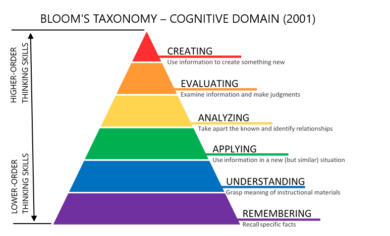
This book is structured with [Bloom’s Taxonomy](https://cft.vanderbilt.edu/guides-sub-pages/blooms-taxonomy/)
in mind ([Figure 1](https://mlsysbook.ai/contents/frontmatter/about/about.html#fig-bloom)
), which defines six levels of learning, ranging from foundational knowledge to advanced creative thinking:
[](https://mlsysbook.ai/contents/frontmatter/about/images/png/bloom_revised_taxonomy.png "Figure 1: Bloom’s Taxonomy (2021 edition).")
Figure 1: Bloom’s Taxonomy (2021 edition).
1. **Remembering**: Recalling basic facts and concepts.
2. **Understanding**: Explaining ideas or processes.
3. **Applying**: Using knowledge in new situations.
4. **Analyzing**: Breaking down information into components.
5. **Evaluating**: Making judgments based on criteria and standards.
6. **Creating**: Producing original work or solutions.
### Learning Objectives
This book supports readers in developing practical expertise across the ML systems lifecycle:
1. **Systems Thinking**: Understand how ML systems differ from traditional software, and reason about hardware-software interactions.
2. **Workflow Engineering**: Design end-to-end ML pipelines, from data engineering through deployment and maintenance.
3. **Performance Optimization**: Apply systematic approaches to make systems faster, smaller, and more resource-efficient.
4. **Production Deployment**: Address real-world challenges including reliability, security, privacy, and scalability.
5. **Responsible Development**: Navigate ethical implications and implement sustainable, socially beneficial AI systems.
6. **Future-Ready Skills**: Develop judgment to evaluate emerging technologies and adapt to evolving paradigms.
7. **Hands-On Implementation**: Gain practical experience across diverse embedded platforms and resource constraints.
8. **Self-Directed Learning**: Use integrated assessments and interactive tools to track progress and deepen understanding.
### AI Learning Companion
Throughout this resource, you’ll find **SocratiQ**, an AI learning assistant designed to enhance your learning experience. Inspired by the Socratic method of teaching, SocratiQ combines interactive quizzes, personalized assistance, and real-time feedback to help you reinforce your understanding and create new connections. As part of our integration of Generative AI technologies, SocratiQ encourages critical thinking and active engagement with the material.
SocratiQ is still a work in progress, and we welcome your feedback to make it better. For more details about how SocratiQ works and how to get the most out of it, visit the [AI Learning Companion page](https://mlsysbook.ai/contents/frontmatter/socratiq/socratiq.html)
.
How to Use This Book
--------------------
### Book Structure
This book takes you from understanding ML systems conceptually to building and deploying them in practice. Each part develops specific capabilities:
**Core Content:**
1. **Foundations** _Master the fundamentals._ Build intuition for how ML systems differ from traditional software, understand the hardware-software stack, and gain fluency with essential architectures and mathematical foundations.
2. **Design Principles** _Engineer complete workflows._ Learn to design end-to-end ML pipelines, manage complex data engineering challenges, select appropriate frameworks, and orchestrate training at scale.
3. **Performance Engineering** _Optimize for real constraints._ Develop skills to make systems faster, smaller, and more efficient through model optimization, hardware acceleration, and systematic performance analysis.
4. **Robust Deployment** _Build production-ready systems._ Progress from individual device constraints through system-wide operations. Master on-device learning, security and privacy as systems scale, robustness against failures, and ML operations that orchestrate production deployment.
5. **Trustworthy Systems** _Design responsibly._ Navigate the social and environmental implications of ML systems, implement responsible AI practices, and create technology that serves the public good.
6. **Frontiers of ML Systems** _Prepare for what’s next._ Understand emerging paradigms, anticipate future challenges, and develop the judgment to evaluate new technologies as they emerge.
**Hands-On Learning:**
7. **Laboratory Exercises** _Implement everything you learn._ Progress from microcontroller-based systems to edge computing platforms, experiencing the full spectrum of resource constraints and optimization challenges in embedded ML.
### Suggested Reading Paths
* **Beginners**: Start with _Foundations_ to build conceptual understanding, then progress through _Design Principles_ and select relevant lab exercises for hands-on experience.
* **Practitioners**: Focus on _Design Principles_, _Performance Engineering_, and _Robust Deployment_ for practical system design insights, complemented by platform-specific lab exercises.
* **Researchers**: Explore _Performance Engineering_, _Trustworthy Systems_, and _ML Systems Frontiers_ for advanced topics, along with comparative analysis from the shared tools lab section.
* **Hands-On Learners**: Combine any core content parts with the comprehensive laboratory exercises across Arduino, Seeed, Grove Vision, and Raspberry Pi platforms for practical implementation experience.
### For Students with Different Backgrounds
This textbook welcomes students from diverse academic backgrounds, whether you come from computer science, engineering, mathematics, or other fields. Understanding how ML systems connect to your existing knowledge helps bridge theoretical concepts to practical implementation:
**Computer Science Students**: ML systems extend familiar concepts into new domains. If you’ve worked with algorithms and data structures, think of ML as learning algorithms that automatically optimize themselves based on data patterns rather than following fixed instructions.
Your experience with system design, memory management, parallel processing, and distributed systems directly applies to ML deployment. The underlying computational complexity analysis still applies—we analyze time and space complexity for training and inference phases separately.
**Electrical and Computer Engineering Students**: ML systems represent a natural evolution of signal processing and control systems principles. Machine learning can be viewed as advanced signal processing where we extract meaningful patterns from noisy, high-dimensional signals.
Neural networks perform operations similar to filters—convolution layers in image processing are literally convolution operations you’ve studied. Your background in computer systems organization and architecture becomes essential for understanding how ML algorithms map to different hardware platforms, while your understanding of memory hierarchies helps optimize data movement in large-scale training systems.
**Students from Other Backgrounds**: Think of ML systems like a modern factory assembly line. Just as a factory transforms raw materials into finished products through coordinated stages, ML systems transform raw data into useful predictions through interconnected components.
The mathematics—linear algebra, probability, and calculus—are the “tools” of this factory, but you don’t need to be a tool expert to understand how the assembly line works. Most concepts become clear through concrete examples, like understanding how a recommendation system works by thinking about how a librarian might suggest books based on your reading history.
The key skill is systems thinking: understanding how data pipelines, training processes, and deployment infrastructure work together, much like how supply chains, manufacturing, and distribution must coordinate in any complex operation.
### Modular Design
The book is designed for flexible learning, allowing readers to explore chapters independently or follow suggested sequences. Each chapter integrates:
* **Interactive quizzes** for self-assessment and knowledge reinforcement
* **Practical exercises** connecting theory to implementation
* **Laboratory experiences** providing hands-on platform-specific learning
We embrace an iterative approach to content development—sharing valuable insights as they become available rather than waiting for perfection. Your feedback helps us continuously improve and refine this resource.
We also build upon the excellent work of experts in the field, fostering a collaborative learning ecosystem where knowledge is shared, extended, and collectively advanced.
Transparency and Collaboration
------------------------------
This book began as a community-driven project shaped by the collective efforts of students in CS249r, colleagues at Harvard and beyond, and the broader ML systems community. Its content has evolved through open collaboration, thoughtful feedback, and modern editing tools—including both rule-based scripts and generative AI technologies. In a fitting twist, the very systems we study in this book have helped refine its pages, highlighting the interplay between human expertise and machine intelligence. Fortunately, they’re not quite ready to engineer the systems themselves—at least, not yet.
As the primary author, editor, and curator, I (Prof. Vijay Janapa Reddi) provide human-in-the-loop oversight to ensure the textbook material remains accurate, relevant, and of the highest quality. Still, no one is perfect—so errors may exist. Your feedback is welcome and encouraged. This collaborative model is essential for maintaining quality and ensuring that knowledge remains open, evolving, and globally accessible.
Copyright and Licensing
-----------------------
This book is open-source and developed collaboratively through GitHub. Unless otherwise stated, this work is licensed under the [Creative Commons Attribution-NonCommercial-ShareAlike 4.0 International (CC BY-NC-SA 4.0)](https://creativecommons.org/licenses/by-nc-sa/4.0)
.
Contributors retain copyright over their individual contributions, dedicated to the public domain or released under the same open license as the original project. For more information on authorship and contributions, visit the [GitHub repository](https://github.com/harvard-edge/cs249r_book)
.
Join the Community
------------------
This textbook is more than just a resource—it’s an invitation to collaborate and learn together. Engage in [community discussions](https://github.com/harvard-edge/cs249r_book/discussions)
to share insights, tackle challenges, and learn alongside fellow students, researchers, and practitioners.
Whether you’re a student starting your journey, a practitioner solving real-world challenges, or a researcher exploring advanced concepts, your contributions will enrich this learning community. Introduce yourself, share your goals, and let’s collectively build a deeper understanding of machine learning systems.
Back to top
---
# ML Systems Textbook
SocratiQ AI
===========
AI Learning Companion
---------------------
Welcome to SocratiQ (pronounced \`\`Socratic’’), an AI learning assistant seamlessly integrated throughout this resource. Inspired by the Socratic method of teaching—emphasizing thoughtful questions and answers to stimulate critical thinking—SocratiQ is part of our experiment with what we call as _Generative Learning._ By combining interactive quizzes, personalized assistance, and real-time feedback, SocratiQ is meant to reinforce your understanding and help you create new connections. _SocratiQ is still a work in progress, and we welcome your feedback._
Learn more: Read our research paper [SocratiQ: A Generative AI-Powered Learning Companion for Personalized Education and Broader Accessibility](https://arxiv.org/abs/2502.00341)
.
Listen to this AI-generated podcast about SocratiQ.
You can enable SocratiQ by clicking the button below:
SocratiQ: OFF
Direct URL Access
You can directly control SocratiQ by adding `?socratiq=` parameters to your URL:
* To activate: [mlsysbook.ai/?socratiq=true](https://mlsysbook.ai/?socratiq=true)
* To deactivate: [mlsysbook.ai/?socratiq=false](https://mlsysbook.ai/?socratiq=false)
This gives you quick access to toggle SocratiQ’s functionality directly from your browser’s address bar, without needing to return here.
SocratiQ’s goal is to adapt to your needs while generating targeted questions and engaging in meaningful dialogue about the material. Unlike traditional textbook study, SocratiQ offers an interactive, personalized learning experience that can help you better understand and retain complex concepts. It is only available as an online feature.
Quick Start Guide
-----------------
1. Enable SocratiQ using the button below or URL parameters
2. Use keyboard shortcut (`Cmd/Ctrl + /`) to open SocratiQ anytime
3. Set your academic level in Settings
4. Start learning! Look for quiz buttons at the end of sections
Please note that this is an experimental feature. We are experimenting with the idea of creating a dynamic and personalized learning experience by harnessing the power of generative AI. We hope that this approach will transform how you interact with and absorb the complex concepts.
Warning
**About AI Responses**: While SocratiQ uses advanced AI to generate quizzes and provide assistance, like all AI systems, it may occasionally provide imperfect or incomplete answers. However, we’ve designed and tested it to ensure it’s effective for supporting your learning journey. If you’re unsure about any response, refer to the textbook content or consult your instructor.
Once you’ve enabled SocratiQ it will always be available when you visit this site.
You can access SocratiQ at any time using a keyboard shortcut shown in [Figure 1](https://mlsysbook.ai/contents/frontmatter/socratiq/socratiq.html#fig-main-shortcut)
, which brings up the interface shown in [Figure 2](https://mlsysbook.ai/contents/frontmatter/socratiq/socratiq.html#fig-main-interface)
.
[](https://mlsysbook.ai/contents/frontmatter/socratiq/images/png/shortcut.png "Figure 1: SocratiQ AI Learning Assistant: The image shows a keyboard shortcut (Ctrl + /) provided for easy access to SocratiQ, demonstrating its integration with users’ environments.")
Figure 1: **SocratiQ AI Learning Assistant**: The image shows a keyboard shortcut (Ctrl + /) provided for easy access to SocratiQ, demonstrating its integration with users’ environments.
[](https://mlsysbook.ai/contents/frontmatter/socratiq/images/png/interface.png "Figure 2: AI Learning Assistant: This image showcases SocratiQ, an AI-powered learning tool designed to enhance understanding of ML systems concepts. The interface features a settings section for academic level, and quiz buttons at the end of sections suggest interactive learning opportunities. SocratiQ serves as an essential tool for computer science students interested in comprehending ML systems concepts.")
Figure 2: **AI Learning Assistant**: This image showcases SocratiQ, an AI-powered learning tool designed to enhance understanding of ML systems concepts. The interface features a settings section for academic level, and quiz buttons at the end of sections suggest interactive learning opportunities. SocratiQ serves as an essential tool for computer science students interested in comprehending ML systems concepts.
Button Overview
---------------
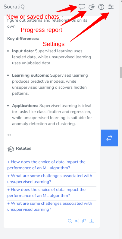
The top nav bar ([Figure 3](https://mlsysbook.ai/contents/frontmatter/socratiq/socratiq.html#fig-top-menu)
) provides quick access to the following features:
1. Adjust your [settings](https://mlsysbook.ai/contents/frontmatter/socratiq/socratiq.html#sec-socratiq-ai-personalize-learning-1d9c)
at any time.
2. Track your [progress](https://mlsysbook.ai/contents/frontmatter/socratiq/socratiq.html#sec-socratiq-ai-tracking-progress-d563)
by viewing the dashboard.
3. Start new or save your [conversations](https://mlsysbook.ai/contents/frontmatter/socratiq/socratiq.html#sec-socratiq-ai-learning-socratiq-d17d)
with SocratiQ.
[](https://mlsysbook.ai/contents/frontmatter/socratiq/images/png/top_menu.png "Figure 3: View of the top nav menu.")
Figure 3: View of the top nav menu.
Personalize Your Learning
-------------------------
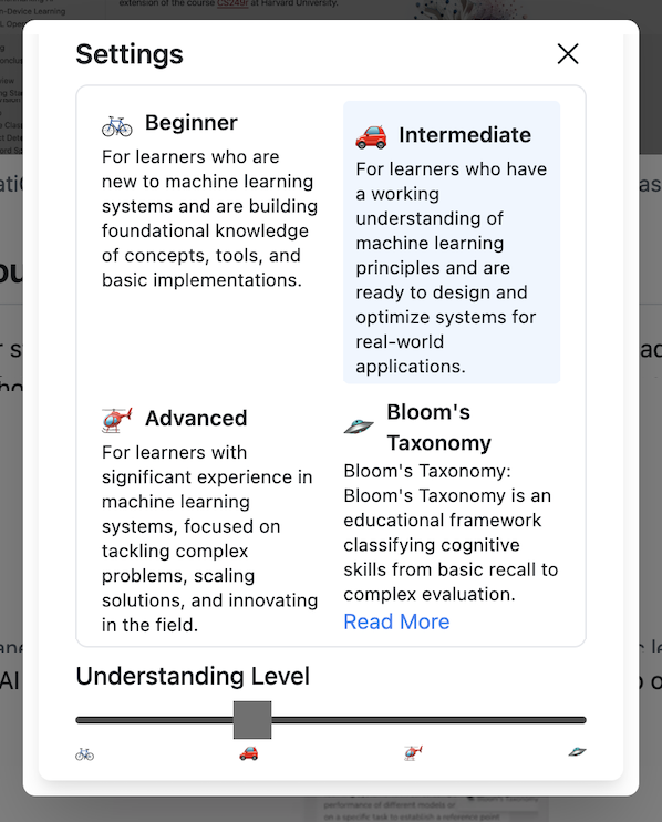
Before diving into your studies, take a moment to configure SocratiQ for your academic level. This initial setup ensures that all interactions, from quiz questions to explanations, are tailored to your background knowledge. [Figure 4](https://mlsysbook.ai/contents/frontmatter/socratiq/socratiq.html#fig-settings-panel)
shows where you can adjust these preferences.
You can augment any AI SocratiQ response using the dropdown menu at the top of each message, allowing you to adjust the difficulty level as shown in [Figure 5](https://mlsysbook.ai/contents/frontmatter/socratiq/socratiq.html#fig-adjust_message_difficulty)
.
[](https://mlsysbook.ai/contents/frontmatter/socratiq/images/png/settings.png "Figure 4: Personalized Learning Preferences: The image shows a user interface that allows for the personalization of an AI-based learning tool, such as SocratiQ, to tailor interactions to the learner’s academic level. The settings panel on the right side of the screen displays options for adjusting preferences in relation to quiz questions and explanations. This customization ensures that the information presented is relevant to the learner’s background knowledge, thereby enhancing understanding of ML systems concepts.")
Figure 4: **Personalized Learning Preferences**: The image shows a user interface that allows for the personalization of an AI-based learning tool, such as SocratiQ, to tailor interactions to the learner’s academic level. The settings panel on the right side of the screen displays options for adjusting preferences in relation to quiz questions and explanations. This customization ensures that the information presented is relevant to the learner’s background knowledge, thereby enhancing understanding of ML systems concepts.
Learning with SocratiQ
----------------------
### Quizzes
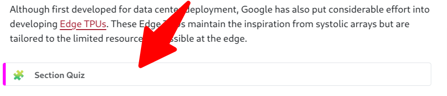
As you progress through each section of the textbook, you have the option to ask SocratiQ to automatically generate quizzes tailored to reinforce key concepts. These quizzes are conveniently inserted at the end of every major subsection (e.g., 1.1, 1.2, 1.3, and so on), as illustrated in [Figure 6](https://mlsysbook.ai/contents/frontmatter/socratiq/socratiq.html#fig-quiz-interface)
. The complete quiz experience, including both questions and answers, is shown in [Figure 7](https://mlsysbook.ai/contents/frontmatter/socratiq/socratiq.html#fig-quizzes)
.
[](https://mlsysbook.ai/contents/frontmatter/socratiq/images/gif/adjust_message_difficulty.gif "Figure 5: AI Response Customization: Redo an AI message by choosing a new experience level.")
Figure 5: **AI Response Customization**: Redo an AI message by choosing a new experience level.
[](https://mlsysbook.ai/contents/frontmatter/socratiq/images/png/quiz_button2.png "Figure 6: AI-Generated Quizzes: This image showcases SocratiQ, an AI-driven learning tool that integrates into a textbook to provide personalized educational experiences for university-level computer science students. By generating tailored quizzes with multiple-choice questions and detailed explanations, SocratiQ facilitates a deeper understanding of ML systems concepts through immediate feedback and adaptive assessments. These quizzes are inserted at the end of major subsections within the textbook material, allowing students to evaluate their comprehension of the preceding sections while reinforcing key concepts. The LLM model employed by SocratiQ enhances student learning and comprehension of ML systems.")
Figure 6: **AI-Generated Quizzes**: This image showcases SocratiQ, an AI-driven learning tool that integrates into a textbook to provide personalized educational experiences for university-level computer science students. By generating tailored quizzes with multiple-choice questions and detailed explanations, SocratiQ facilitates a deeper understanding of ML systems concepts through immediate feedback and adaptive assessments. These quizzes are inserted at the end of major subsections within the textbook material, allowing students to evaluate their comprehension of the preceding sections while reinforcing key concepts. The LLM model employed by SocratiQ enhances student learning and comprehension of ML systems.
Each quiz typically consists of 3-5 multiple-choice questions and takes only 1-2 minutes to complete. These questions are designed to assess your understanding of the material covered in the preceding section, as shown in [Figure 7 (a)](https://mlsysbook.ai/contents/frontmatter/socratiq/socratiq.html#fig-quiz-questions)
.
Upon submitting your answers, SocratiQ provides immediate feedback along with detailed explanations for each question, as demonstrated in [Figure 7 (b)](https://mlsysbook.ai/contents/frontmatter/socratiq/socratiq.html#fig-quiz-answers)
.
[](https://mlsysbook.ai/contents/frontmatter/socratiq/images/png/quiz_questions.png "Figure 7 (a): AI-Generated Personalized Quizzes: This image showcases an AI-driven learning tool called SocratiQ that provides university-level computer science students with a tailored educational experience to facilitate a deeper understanding of ML systems concepts through interactive, personalized quizzes. Integrated into the textbook material, these quizzes comprise multiple-choice questions and detailed explanations for each answer, designed to assess comprehension of the preceding sections and reinforce key concepts using immediate feedback. SocratiQ employs a Large Language Model (LLM) to automatically generate and grade these adaptive quizzes, providing students with an educational experience that enhances their learning and comprehension of ML systems.")
(a) **AI-Generated Personalized Quizzes**: This image showcases an AI-driven learning tool called SocratiQ that provides university-level computer science students with a tailored educational experience to facilitate a deeper understanding of ML systems concepts through interactive, personalized quizzes. Integrated into the textbook material, these quizzes comprise multiple-choice questions and detailed explanations for each answer, designed to assess comprehension of the preceding sections and reinforce key concepts using immediate feedback. SocratiQ employs a Large Language Model (LLM) to automatically generate and grade these adaptive quizzes, providing students with an educational experience that enhances their learning and comprehension of ML systems.
[](https://mlsysbook.ai/contents/frontmatter/socratiq/images/png/quiz_answers.png "Figure 7 (b): AI-Generated Personalized Quizzes: This image showcases an AI-driven learning tool called SocratiQ that provides university-level computer science students with tailored educational experiences through interactive, personalized quizzes. Integrated into the textbook material, these quizzes facilitate a deeper understanding of ML systems concepts by reinforcing key concepts using immediate feedback and adaptive assessments. Each quiz typically consists of 3-5 multiple-choice questions and takes only 1-2 minutes to complete.")
(b) **AI-Generated Personalized Quizzes**: This image showcases an AI-driven learning tool called SocratiQ that provides university-level computer science students with tailored educational experiences through interactive, personalized quizzes. Integrated into the textbook material, these quizzes facilitate a deeper understanding of ML systems concepts by reinforcing key concepts using immediate feedback and adaptive assessments. Each quiz typically consists of 3-5 multiple-choice questions and takes only 1-2 minutes to complete.
Figure 7: SocratiQ uses a Large Language Model (LLM) to automatically generate and grade quizzes.
### Example Learning Flow
1. Read a section
2. Select challenging text → Ask SocratiQ for explanation
3. Take the section quiz
4. Review related content suggestions
5. Track progress in dashboard
### Getting Help with Concepts
When you encounter challenging concepts, SocratiQ offers two powerful ways to get help. First, you can select any text from the textbook and ask for a detailed explanation, as demonstrated in [Figure 8](https://mlsysbook.ai/contents/frontmatter/socratiq/socratiq.html#fig-text-selection)
.
[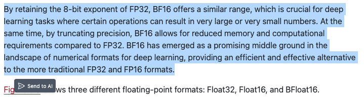](https://mlsysbook.ai/contents/frontmatter/socratiq/images/png/chat_context.png "Figure 8: AI-Assisted Learning Tool: SocratiQ: The image showcases an AI-powered learning tool called SocratiQ that assists university-level computer science students in deepening their understanding of challenging Machine Learning (ML) concepts. By selecting any portion of the textbook and asking for a detailed explanation, students can access personalized, interactive assistance tailored to their learning objectives, fostering self-directed learning and critical thinking skills. SocratiQ provides suggestions for related content from the textbook and guides users through complex ML topics with ease.")
Figure 8: **AI-Assisted Learning Tool: SocratiQ**: The image showcases an AI-powered learning tool called SocratiQ that assists university-level computer science students in deepening their understanding of challenging Machine Learning (ML) concepts. By selecting any portion of the textbook and asking for a detailed explanation, students can access personalized, interactive assistance tailored to their learning objectives, fostering self-directed learning and critical thinking skills. SocratiQ provides suggestions for related content from the textbook and guides users through complex ML topics with ease.
Once you’ve selected the text, you can ask questions about it, and SocratiQ will provide detailed explanations based on that context, as illustrated in [Figure 9](https://mlsysbook.ai/contents/frontmatter/socratiq/socratiq.html#fig-context-explanation)
.
[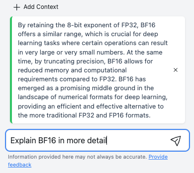](https://mlsysbook.ai/contents/frontmatter/socratiq/images/png/chat_ask.png "Figure 9: AI-Assisted Learning Tool: SocratiQ: The image showcases an AI-powered learning tool called SocratiQ that assists university-level computer science students in deepening their understanding of challenging Machine Learning (ML) concepts. By selecting any portion of the textbook and asking for a detailed explanation, students can access personalized, interactive assistance tailored to their learning objectives, fostering self-directed learning and critical thinking skills. SocratiQ provides suggestions for related content from the textbook and guides users through complex ML topics with ease.")
Figure 9: **AI-Assisted Learning Tool: SocratiQ**: The image showcases an AI-powered learning tool called SocratiQ that assists university-level computer science students in deepening their understanding of challenging Machine Learning (ML) concepts. By selecting any portion of the textbook and asking for a detailed explanation, students can access personalized, interactive assistance tailored to their learning objectives, fostering self-directed learning and critical thinking skills. SocratiQ provides suggestions for related content from the textbook and guides users through complex ML topics with ease.
[Figure 11](https://mlsysbook.ai/contents/frontmatter/socratiq/socratiq.html#fig-interactive-chat)
shows the response for the ask in [Figure 9](https://mlsysbook.ai/contents/frontmatter/socratiq/socratiq.html#fig-context-explanation)
.
[](https://mlsysbook.ai/contents/frontmatter/socratiq/images/gif/reference.gif "Figure 10: Referencing different sections from the textbook.")
Figure 10: Referencing different sections from the textbook.
Additionally, you can also reference Sections, as shown in [Figure 10](https://mlsysbook.ai/contents/frontmatter/socratiq/socratiq.html#fig-reference-sections)
, Sub-sections and keywords directly as you converse with SocratiQ. Use the `@` symbol to reference a section, sub-section or keyword. You can also click the `+ Context` button right above the input.
[](https://mlsysbook.ai/contents/frontmatter/socratiq/images/png/chat_explanation.png "Figure 11: AI-Assisted Learning Tool: The image illustrates an innovative AI-powered learning tool called SocratiQ that assists university-level computer science students in enhancing their understanding of challenging Machine Learning (ML) concepts. By selecting any portion of the textbook and asking for a detailed explanation, students can access personalized, interactive assistance tailored to their learning objectives. This promotes self-directed learning and critical thinking skills by offering suggestions for related content from the textbook and guiding users through complex ML topics with ease. SocratiQ fosters deep understanding of ML systems by providing detailed explanations based on selected context.")
Figure 11: **AI-Assisted Learning Tool**: The image illustrates an innovative AI-powered learning tool called SocratiQ that assists university-level computer science students in enhancing their understanding of challenging Machine Learning (ML) concepts. By selecting any portion of the textbook and asking for a detailed explanation, students can access personalized, interactive assistance tailored to their learning objectives. This promotes self-directed learning and critical thinking skills by offering suggestions for related content from the textbook and guiding users through complex ML topics with ease. SocratiQ fosters deep understanding of ML systems by providing detailed explanations based on selected context.
To enhance your learning experience, SocratiQ doesn’t just answer your questions, it also suggests related content from the textbook that might be helpful for deeper understanding, as shown in [Figure 12](https://mlsysbook.ai/contents/frontmatter/socratiq/socratiq.html#fig-related-content)
.
[](https://mlsysbook.ai/contents/frontmatter/socratiq/images/png/chat_related.png "Figure 12: SocratiQ AI-Assisted Learning Tool: An AI-powered learning tool designed for university-level computer science students to enhance their understanding of challenging Machine Learning (ML) concepts. By selecting any portion of the textbook and asking for a detailed explanation, students can access personalized, interactive assistance tailored to their learning objectives, fostering self-directed learning and critical thinking skills. The AI tool enhances learning by providing suggestions for related content from the textbook and guiding users through complex ML topics with ease.")
Figure 12: **SocratiQ AI-Assisted Learning Tool**: An AI-powered learning tool designed for university-level computer science students to enhance their understanding of challenging Machine Learning (ML) concepts. By selecting any portion of the textbook and asking for a detailed explanation, students can access personalized, interactive assistance tailored to their learning objectives, fostering self-directed learning and critical thinking skills. The AI tool enhances learning by providing suggestions for related content from the textbook and guiding users through complex ML topics with ease.
Tracking Your Progress
----------------------
### Performance Dashboard
SocratiQ maintains a comprehensive record of your learning journey. The progress dashboard ([Figure 13](https://mlsysbook.ai/contents/frontmatter/socratiq/socratiq.html#fig-progress-dashboard)
) displays your quiz performance statistics, learning streaks, and achievement badges. This dashboard updates in real-time.
[](https://mlsysbook.ai/contents/frontmatter/socratiq/images/png/dashboard.png "Figure 13: AI-Assisted Learning Dashboard: The image depicts SocratiQ’s performance dashboard, an AI-assisted learning platform that enables students to track their progress in mastering ML systems concepts. The dashboard displays key statistics such as quiz performance, learning streaks, and achievement badges. By engaging consistently with the material, students can earn various badges that recognize their progress and reinforce their understanding of essential ML concepts. These features help students monitor their learning journey, visualize their growth, and motivate themselves towards continuous improvement.")
Figure 13: **AI-Assisted Learning Dashboard**: The image depicts SocratiQ’s performance dashboard, an AI-assisted learning platform that enables students to track their progress in mastering ML systems concepts. The dashboard displays key statistics such as quiz performance, learning streaks, and achievement badges. By engaging consistently with the material, students can earn various badges that recognize their progress and reinforce their understanding of essential ML concepts. These features help students monitor their learning journey, visualize their growth, and motivate themselves towards continuous improvement.
As you continue to engage with the material and complete quizzes, you’ll earn various badges that recognize your progress, as shown in [Figure 14](https://mlsysbook.ai/contents/frontmatter/socratiq/socratiq.html#fig-achievement-badges)
.
[](https://mlsysbook.ai/contents/frontmatter/socratiq/images/png/badges.png "Figure 14: AI-Assisted Learning Dashboard: SocratiQ’s performance dashboard is an AI-assisted learning platform that enables students to track their progress in mastering ML systems concepts. By engaging consistently with the material, students can earn various achievement badges that recognize their progress and reinforce their understanding of essential ML concepts. The dashboard displays key statistics such as quiz performance, learning streaks, and achievement badges.")
Figure 14: **AI-Assisted Learning Dashboard**: SocratiQ’s performance dashboard is an AI-assisted learning platform that enables students to track their progress in mastering ML systems concepts. By engaging consistently with the material, students can earn various achievement badges that recognize their progress and reinforce their understanding of essential ML concepts. The dashboard displays key statistics such as quiz performance, learning streaks, and achievement badges.
### Achievement Badges
As you progress through the quizzes, you’ll earn special badges to mark your achievements! Here’s what you can earn:
| | | |
| --- | --- | --- |
|  | First Steps | Complete your first quiz |
|  | On a Streak | Maintain a streak of perfect scores |
|  | Quiz Medalist | Complete 10 quizzes |
|  | Quiz Champion | Complete 20 quizzes |
|  | Quiz Legend | Complete 30 quizzes |
|  x n | Quiz AGI Super Human | Complete 40 or more quizzes |
Tip
Keep taking quizzes to collect all badges and improve your learning journey! Your current badges will appear in the quiz statistics dashboard.
If you’d like a record of your progress you can generate a PDF report ([Figure 15](https://mlsysbook.ai/contents/frontmatter/socratiq/socratiq.html#fig-download-report)
). It will show your progress, average performance and all the questions you’ve attempted. The PDF is a generated with a unique hash and can be uniquely validated.
Data Storage
------------
Important
**Important Note**: All progress data is stored locally in your browser. Clearing your browser history or cache will erase your entire learning history, including quiz scores, streaks, and achievement badges.
You can also delete all of your saved conversations by clicking the New Chat button in the nav bar, as shown in [Figure 16](https://mlsysbook.ai/contents/frontmatter/socratiq/socratiq.html#fig-previous-conversations)
.
Technical Requirements
----------------------
To use SocratiQ effectively, you’ll need:
* Chrome or Safari browser
* JavaScript enabled
* Stable internet connection
[](https://mlsysbook.ai/contents/frontmatter/socratiq/images/png/download_report.png "Figure 15: You can click the Download Report button to view your report. You can verify that your PDF has been created by SocratiQ by clicking the verify button and uploading your generated PDF.")
Figure 15: You can click the Download Report button to view your report. You can verify that your PDF has been created by SocratiQ by clicking the verify button and uploading your generated PDF.
[](https://mlsysbook.ai/contents/frontmatter/socratiq/images/png/prev_conversations.png "Figure 16: Load or delete previous chats or start a new chat.")
Figure 16: Load or delete previous chats or start a new chat.
Common Issues and Troubleshooting
---------------------------------
* If SocratiQ isn’t responding: Refresh the page
* If quizzes don’t load: Check your internet connection
* If progress isn’t saving: Ensure cookies are enabled
For persistent issues, please contact us at vj\[@\]eecs.harvard.edu.
Providing Feedback
------------------
Your feedback helps us improve SocratiQ.
You can report technical issues, suggest improvements to quiz questions, or share thoughts about AI responses using the feedback buttons located throughout the interface. You can submit a [GitHub issue](https://github.com/harvard-edge/cs249r_book/issues)
.
Back to top
---
# ML Systems Textbook
Book Changelog
==============
This Machine Learning Systems textbook is constantly evolving. This changelog is intended to record all updates and improvements, helping you stay informed about what’s new and refined.
Automated Changelog
These changelog entries are automatically generated from our development process and should be mostly accurate. They track code changes, content updates, and improvements across the entire book. While the entries are comprehensive, they may occasionally contain minor inaccuracies or overly technical details.
2025 Updates
------------
### 📅 December 11
**📄 Frontmatter**
* `█████` **Acknowledgements**: The acknowledgements section was updated multiple times to reflect changes in contributor lists.Additionally, a fix was implemented to ensure XHTML compliance in frontmatter files, specifically addressing an issue with ebook loading and display errors.
* `██░░░` **Foreword**: This commit addresses an issue with epub generation by ensuring that the Foreword file (foreword.qmd) complies with XHTML standards. This helps to maintain consistency and compatibility across different platforms.
* `██░░░` **Changelog**: This commit focuses on improving the Epub output by ensuring XHTML compliance in frontmatter files. This helps maintain document integrity and consistency for users accessing the content in Epub format.
* `██░░░` **SocratiQ**: This update ensures that SocratiQ’s frontmatter files comply with XHTML standards, improving ePub compatibility and readability.
* `█░░░░` **Index**: This commit focuses on ensuring XHTML compliance within frontmatter files for epub output, fixing potential issues related to markup validity.
**📖 Chapters**
* `█████` **Chapter 6: Data Engineering**: Chapter 6, “Data Engineering,” was updated with several improvements. This included fixing typos, standardizing definition titles, and revising definitions for “lifecycle” and “operations” to ensure consistency.
* `█████` **Chapter 20: Frontiers**: The “Frontiers” chapter received several updates, including improved math formatting, the addition of a chain-of-thought citation, expanded discussion on artificial general intelligence (AGI), and standardized definition titles. Additionally, benchmarking and AGI definitions were revised to a canonical form for clarity and consistency.
* `████░` **Chapter 1: Introduction**: Chapter 1 received updates to clarify foundational definitions, refine explanations of deep learning and data drift, and improve sentence structure for clarity. Additional changes included fixing typos and addressing formatting issues.
* `████░` **Chapter 3: DL Primer**: The Chapter 3 DL Primer was updated with several improvements, including correcting errors in weight matrix calculations and forward propagation, standardizing mathematical conventions, and adding missing definitions for key concepts like Backpropagation and Gradient Descent. Additional changes focused on improving clarity, removing redundancies, and ensuring consistent terminology throughout the chapter.
* `███░░` **Chapter 2: ML Systems**: Chapter 2 on ML Systems received several improvements, including standardized formatting for definition titles, revised deployment paradigm definitions for clarity, and the correction of typos throughout the chapter. These changes enhance readability and accuracy within the ML Systems content.
* `███░░` **Chapter 4: DNN Architectures**: The commit messages indicate updates to Chapter 4 focusing on consistency and clarity. Key changes include standardizing matrix multiplication conventions, refining definitions for academic tone, and revising neural architecture definitions for a more consistent format.
* `███░░` **Chapter 8: AI Training**: Chapter 8’s AI training content was enhanced with missing definitions for Tier 1 and Tier 2 categories. Additionally, the existing definitions were standardized in format and revised to ensure clarity and consistency.
* `███░░` **Chapter 10: Model Optimizations**: This update focuses on refining the content in Chapter 10 by correcting typos across several files and standardizing the formatting of definitions related to hardware and optimization techniques.The chapter now features a more consistent and accurate presentation of key terms.
* `███░░` **Chapter 11: AI Acceleration**: This update focuses on refining content accuracy and consistency in Chapter 11. Key changes include fixing typos, standardizing definition titles, revising hardware and optimization definitions for clarity, and verifying bibliographic information.
* `██░░░` **Chapter 5: AI Workflow**: Chapter 5’s AI Workflow now includes all Tier 1 and Tier 2 definitions, with standardized titles for clarity. Additionally, definitions related to “lifecycle” and “operations” have been revised to ensure consistency and accuracy.
* `██░░░` **Chapter 7: AI Frameworks**: Chapter 7 on AI Frameworks was updated with several improvements, including fixing typos and standardizing definition titles. Most importantly, key definitions for Tier 1 and Tier 2 frameworks were added and existing lifecycle and operations definitions were revised to a canonical format for clarity.
* `██░░░` **Chapter 12: Benchmarking AI**: This update focuses on clarifying key concepts within Chapter 12. It corrects typos across three files and revises the definitions of “benchmarking” and “AGI” for greater consistency and accuracy.
* `██░░░` **Chapter 13: ML Operations**: The ML Operations chapter was updated with standardized definition titles and revised lifecycle and operations definitions for clarity and consistency. Minor typographical errors were also corrected in the document.
* `██░░░` **Chapter 14: On-Device Learning**: The commit messages indicate that the definitions section in Chapter 14 was updated. Specifically, the titles of definitions were standardized and the descriptions of deployment paradigms were revised for clarity and consistency.
* `██░░░` **Chapter 15: Security & Privacy**: Chapter 15’s content on privacy and security has been updated with standardized formatting for definition titles and revised definitions for the Responsible AI suite. These changes improve clarity and consistency in the documentation.
* `██░░░` **Chapter 19: AI for Good**: This update focuses on improving clarity and accuracy in Chapter 19. It standardizes definition titles, revises definitions for the Responsible AI suite to be more consistent, and ensures all bibliographic entries have valid DOIs.
* `█░░░░` **Chapter 9: Efficient AI**: This update streamlines Chapter 9 by standardizing the format for definition titles and revising the wording of key terms related to hardware and optimization techniques within the “Efficient AI” section. These changes improve clarity and consistency in the presentation of essential concepts.
* `█░░░░` **Chapter 16: Robust AI**: This update standardizes the formatting for definition titles within Chapter 16 and revises the definitions related to the “Responsible AI Suite” to ensure consistency and clarity.
* `█░░░░` **Chapter 17: Responsible AI**: The “Responsible AI” chapter in Quarto saw improvements to its definition section. This included standardizing the formatting of definition titles and revising the Responsible AI suite definitions for clarity and consistency.
* `█░░░░` **Chapter 18: Sustainable AI**: This update standardizes the formatting of definition titles within Chapter 18 and revises the definitions for the Responsible AI suite to ensure consistency and clarity.
**🧑💻 Labs**
* `██░░░` **Lab: Labs**: This commit improves the Lab ebook by converting more `.qmd` file path links within the `labs.qmd` document into section references, enhancing navigation and readability for users.
* `██░░░` **Lab: Nicla Vision**: This update improves the Nicla Vision Lab documentation by converting file-path links within the lab overviews to section references in ePub format. This change enhances navigation and readability for users accessing the lab through ePub publications.
* `█░░░░` **Lab: Arduino Object Detection**: This update fixes several typos found across three files related to the Arduino object detection lab. These corrections ensure the accuracy and clarity of the provided information for users.
* `█░░░░` **Lab: Arduino Keyword Spotting**: This update addresses typos found within the Lab: Arduino Keyword Spotting documentation, ensuring accuracy and clarity for users.
* `█░░░░` **Lab: Arduino Motion Classification**: This commit addresses typos found in two files within the “Arduino Motion Classification” lab content. The corrections ensure accuracy and clarity in the provided instructions and explanations.
* `███░░` **Lab: Xiao Esp32S3**: This update fixes an issue with file-path links in the Xiao ESP32S3 Lab’s overview sections. It converts these links to section references for improved navigation and readability within the ePub format.
* `█░░░░` **Lab: Arduino Image Classification**: This commit fixes minor typos found within the “labs” section of the documentation.
* `██░░░` **Lab: Arduino Keyword Spotting**: This update addresses two issues in the Lab: Arduino Keyword Spotting content. It ensures remote resources are handled correctly within ePub output and removes the deprecated `frameborder` attribute from iframes for improved compatibility.
* `██░░░` **Lab: Arduino Motion Classification**: This update focuses on improving the Lab’s readability and accuracy.It fixes typographical errors in the “labs” section and converts file path links within .qmd files to section references for better navigation in epub format.
* `███░░` **Lab: Grove Vision Ai V2**: The Lab: Grove Vision Ai V2 content was updated to clearly indicate that object detection is still under development (TBD). Additionally, file path links within lab overviews were replaced with section references for improved readability in epub format.
* `█░░░░` **Lab: Arduino Image Classification**: Two commits addressed minor issues within the “image\_classification” lab. They focused on correcting typos across three files and then two additional files, ensuring accuracy and clarity in the content.
* `███░░` **Lab: Raspi**: This commit improves the Lab: Raspi Qmd file by fixing how file path links are handled in overviews. It now converts these links to section references, enhancing readability and navigation within the document.
* `█░░░░` **Lab: Arduino Setup**: This update fixes several typos found across three different files within the Arduino Setup Lab documentation.
* `█░░░░` **Lab: Arduino Image Classification**: The image classification lab now uses the correct URL to download the “labels.txt” file. This fix ensures the lab functions as intended by providing the necessary data for image recognition.
* `███░░` **Lab: Arduino Object Detection**: This update addresses numerous typos throughout the Arduino Object Detection lab, particularly focusing on corrections related to the Raspberry Pi instructions and the spelling of the Ultralytics library. These fixes enhance the clarity and accuracy of the lab materials.
* `██░░░` **Lab: Pi Vision Language Models**: This update focused on improving the clarity and accuracy of the Lab: Pi Vision Language Models documentation.Several typos were corrected across various files within the labs section, ensuring the content is now free of grammatical errors and presents information accurately.
**🔧 Infrastructure**
* `█████` **TinyTorch Integration**: TinyTorch, the companion hands-on learning platform, has been integrated into the MLSysBook repository as a monorepo. This includes dedicated CI/CD workflows, the Tito CLI tool for module management, and streamlined deployment configurations.
### 📅 November 02
**📄 Frontmatter**
* `█████` **Acknowledgements**: The acknowledgements section was updated to include new contributors, remove outdated entries, and refine contributor information. Additionally, SVG logos were converted to PNG format for better display and Netlify and Edge Impulse were added as corporate supporters.
* `████░` **About**: This update refactors the About section with clearer section labels and improved CLI help. It also reorganizes Part IV content, enhances pedagogical philosophy, implements classroom feedback improvements, and streamlines directory structure for better navigation.
* `███░░` **Index**: This update focuses on improving the structure and navigation of the book. It adds section IDs to all headers, including chapters, and refines the content related to AI systems engineering.
* `███░░` **Foreword**: The foreword’s content has been refined to provide a more comprehensive overview of AI systems engineering principles and practices. This update aims to enhance the introduction to the subject matter for readers.
* `███░░` **SocratiQ**: This update focuses on enhancing the clarity and readability of the SocratiQ documentation. It includes improvements to image descriptions, functionality explanations, markdown rendering, and visibility conditions for different sections.
* `██░░░` **Changelog**: The changelog now has improved visibility logic, dynamically adjusting its display based on specific formats and content types. These updates enhance the flexibility and accuracy of how the changelog is presented.
**📖 Chapters**
* `█████` **Chapter 1: Introduction**: The “Introduction” chapter was significantly revised, clarifying the distinction between machine learning and traditional software, incorporating expert feedback, and refining the narrative flow for a smoother reading experience. Key updates also include improvements to callout definitions, footnote systems, and the overall explanation of training-serving skew.
* `█████` **Chapter 2: ML Systems**: Chapter 2, “ML Systems,” underwent significant revisions focusing on clarity, accuracy, and narrative flow. Updates include streamlined content, improved table formatting, refined learning objectives, and enhanced cross-references for better integration with other chapters.
* `█████` **Chapter 3: DL Primer**: The Chapter 3 update focused on refining content clarity and narrative flow, including improvements to the DL Primer section, standardizing learning objectives formatting, and addressing Windows PDF build errors. Various stylistic refinements and cross-reference updates were also implemented.
* `█████` **Chapter 4: DNN Architectures**: The Chapter 4 DNN Architectures update focuses on improving content clarity, readability, and flow by incorporating expert feedback, refining section order, and standardizing formatting. Additionally, new TikZ figures enhance visual explanations and pedagogical effectiveness.
* `█████` **Chapter 5: AI Workflow**: The Chapter 5: AI Workflow was significantly revised to improve clarity, flow, and learning objectives alignment. Updates include formatting fixes, cross-reference standardization, refined content based on expert feedback, and the addition of concept maps and callout definitions.
* `█████` **Chapter 6: Data Engineering**: The Data Engineering chapter was significantly improved with enhanced flow, narrative improvements, the addition of equations and citations, and a four pillars diagram. Formatting and content were also refined across all chapters based on expert feedback and pre-commit validation.
* `█████` **Chapter 7: AI Frameworks**: Chapter 7 on AI Frameworks was significantly revised with improvements to clarity, flow, formatting, and content accuracy. Key changes include standardized learning objectives, updated content reflecting ML Systems Engineering principles, and enhanced cross-references for better navigation.
* `█████` **Chapter 8: AI Training**: The Chapter 8 “AI Training” content was significantly refined with enhancements to learning objectives, formatting, flow, and integration with other chapters. This update also incorporated student feedback and expert insights for a more comprehensive and impactful learning experience.
* `█████` **Chapter 9: Efficient AI**: Chapter 9 on Efficient AI received significant updates, including streamlining content for clarity and flow, addressing repetitive information, and enhancing the learning experience through improved cross-references, concept maps, and callout definitions. Additionally, formatting and technical aspects were refined for a polished final product.
* `█████` **Chapter 10: Model Optimizations**: Chapter 10 on Model Optimizations was significantly revised with improvements to clarity, formatting, and content accuracy. This included addressing typos, updating figures, refining explanations, and standardizing the chapter’s structure.
* `█████` **Chapter 11: AI Acceleration**: Chapter 11 on AI Acceleration was significantly improved with updates to its content, flow, organization, and cross-chapter integration. Key changes include enhanced architectural explanations, refined learning objectives, and the addition of new footnotes for deeper understanding.
* `█████` **Chapter 12: Benchmarking AI**: Chapter 12 on Benchmarking AI was significantly revised, including improvements to clarity, content accuracy, and integration with other chapters. Key changes include addressing reader feedback on performance vs. energy efficiency, adding new TikZ figures, and refining the overall flow and organization of the chapter.
* `█████` **Chapter 13: ML Operations**: Chapter 13 on ML Operations was significantly revised, including improvements to flow, additions of new content like infrastructure as code and stakeholder communication, and refinements to existing sections for clarity and consistency. The chapter also incorporates feedback and updates based on pre-commit fixes and expert reviews.
* `█████` **Chapter 14: On-Device Learning**: Chapter 14 on On-Device Learning was significantly improved with content refinements, enhanced learning objectives, and the addition of new TikZ figures based on student feedback. Several technical fixes and formatting updates were also implemented across the chapter.
* `█████` **Chapter 15: Security & Privacy**: Chapter 15 on Security & Privacy was significantly updated with improvements to content flow, pedagogical techniques, and added decision frameworks. Key changes include enhanced learning objectives, concrete examples, and a refined narrative arc for improved understanding.
* `█████` **Chapter 18: Robust AI**: The Chapter 18: Robust AI update focused on enhancing clarity and narrative flow by elaborating on concepts like adversarial examples and dropout, alongside refinements to formatting and content organization. Additionally, several typos were corrected for improved accuracy.
* `█████` **Chapter 16: Responsible AI**: The Responsible AI chapter received significant enhancements, including improved flow, added scenarios, and pedagogical improvements. Overall, various chapters were refined with clearer language, consistent formatting, and enhanced learning objectives across the entire textbook.
* `█████` **Chapter 17: Sustainable AI**: Chapter 17 on Sustainable AI received comprehensive updates, including improved flow, enhanced learning objectives, incorporated expert feedback, refined formatting, and the addition of content on carbon footprint tracking and optical interconnects. Numerous smaller fixes and improvements were also made to ensure clarity, consistency, and accuracy.
* `█████` **Chapter 19: AI for Good**: Chapter 19, “AI for Good,” underwent significant revisions focusing on content clarity, flow, and integration with other chapters. This included addressing cross-references, refining learning objectives, and incorporating expert feedback to enhance the chapter’s overall quality and coherence.
* `█████` **Chapter 20: Frontiers**: Chapter 20, “Frontiers,” was significantly enhanced with improved flow, coherence, and conceptual progression. Key updates include standardized learning objectives, revised content incorporating expert feedback, comprehensive citations, and optimized cross-references for better navigation.
* `█████` **Lab: Conclusion**: The conclusion chapter was refactored to focus on principles rather than a chronological review. Extensive revisions were made across all chapters, including content updates, formatting improvements, and the addition of concept maps and optimized cross-references.
* `█████` **Glossary**: This update significantly improves the Glossary section by standardizing labels, removing redundancies, and implementing Quarto cross-reference links for better navigation. It also includes additions of key AGI terms and refactors the glossary scripts for improved organization and data flow.
* `████░` **Chapter: Emerging Topics**: This update refactored the project structure by removing the “emerging\_topics” directory and improved cross-referencing throughout the textbook. Key additions include concept maps for all chapters and section IDs for headers, enhancing navigation and comprehension.
* `███░░` **Chapter: Generative Ai**: This update enhances the Generative AI chapter with improved organization, cross-referencing, and concept mapping. It also optimizes flow while preserving engineering insights and addressing conceptual dependencies.
* `██░░░` **PhD Survival Guide**: This update applies unique section IDs to all headers within the PhD Survival Guide, including chapters, enhancing navigation and accessibility for readers.
* `█░░░░` **Foundations**: This commit improves the structure and usability of Foundations documentation by applying unique section IDs to all headers, including chapters. This change enhances readability and makes it easier for users to navigate and reference specific content using the CLI.
* `█░░░░` **Best Practices**: This update applies section IDs to all headers within the Best Practices document, including chapter headings, improving navigation and accessibility.
* `█░░░░` **Design Principles**: This commit improves navigation by applying unique section IDs to all headers, including chapter headings, in the Design Principles document. This enhancement allows for easier linking and referencing within the document.
* `█░░░░` **Impact Outlook**: This update applies section IDs to all headers in Impact Outlook, including chapter headings, improving navigation and searchability within the document.
**🧑💻 Labs**
* `███░░` **Lab: Labs**: This update improves the readability and structure of the Labs documentation. It includes fixing Markdown formatting, standardizing table styles, and adding section IDs to all headers for easier navigation.
* `████░` **Lab: Kits**: This update improves the visual consistency of Lab: Kits by standardizing table formatting and applying section IDs to all headers, making navigation easier. Additional changes include refining script names for clarity and updating internal links.
* `████░` **Lab: Ide Setup**: This update improves the readability and organization of the IDE setup lab by adding blank lines after list headings for better formatting. It also enhances navigation by applying section IDs to all headers, including chapters, making it easier to link between different parts of the document.
* `██░░░` **Lab: Nicla Vision**: This update improves the Lab: Nicla Vision content by adding section IDs to all headers, including chapters, for easier navigation. It also refactors the content with updated section labels and enhances the command-line interface (CLI) help for better user experience.
* `███░░` **Lab: Arduino Setup**: This update focuses on improving clarity and readability within the Arduino Setup lab. It fixes typos throughout the text, clarifies the description of IMU data, and adds section IDs to all headers for easier navigation.
* `███░░` **Lab: Arduino Image Classification**: This update enhances the Lab: Arduino Image Classification document by adding section IDs to all headers, including chapters, improving navigation and searchability. It also includes unspecified content and configuration file updates.
* `████░` **Lab: Arduino Object Detection**: This update focuses on refining the quality and readability of the Arduino Object Detection lab. It includes typo corrections, formatting improvements based on expert feedback, content updates, and the implementation of section IDs for better navigation.
* `███░░` **Lab: Arduino Keyword Spotting**: This update improves organization and readability within the lab content by applying section IDs to all headers, including chapters. Additionally, script names have been standardized for better clarity and maintainability.
* `███░░` **Lab: Arduino Motion Classification**: This update enhances readability and organization within the lab by applying section IDs to all headers, including chapters. Additionally, it standardizes script naming conventions in the scripts folder for improved clarity and maintainability.
* `███░░` **Lab: Xiao Esp32S3**: This commit batch refactors the lab content by updating section labels, improving CLI help messages, formatting tables consistently, and applying section IDs to all headers for better navigation.
* `████░` **Lab: Arduino Setup**: This commit improves the Lab: Arduino Setup guide by adding section IDs to all headers, ensuring proper navigation. It also fixes image references and updates links for consistency and usability.
* `█████` **Lab: Arduino Image Classification**: This commit introduces several improvements to the Arduino Image Classification lab, including updated image filenames, standardized script naming conventions, and enhanced code highlighting. It also incorporates changes for better readability and navigation within the lab content.
* `████░` **Lab: Arduino Object Detection**: This commit focuses on improving file organization and image referencing within the lab content. It renames auto-generated images, downloads external images, standardizes filename casing, and applies section IDs to headers for better navigation.
* `█████` **Lab: Arduino Keyword Spotting**: This commit batch focuses on improving readability and accuracy within the Arduino Keyword Spotting lab. Key changes include fixing typos, renaming images for clarity, updating image references, applying section IDs to headers, and incorporating updates based on a new kit.
* `███░░` **Lab: Arduino Motion Classification**: This commit improves readability and consistency in the Lab document. It fixes typos, applies section IDs to all headers for easier navigation, and standardizes image filenames for accurate referencing.
* `███░░` **Lab: Grove Vision Ai V2**: This commit focuses on enhancing the clarity and structure of the Grove Vision Ai V2 lab documentation. It standardizes section labels, improves CLI help messages, formats tables consistently, and applies unique IDs to all headers for easier navigation.
* `███░░` **Lab: Setup And No Code Apps**: This update improves organization by applying section IDs to all headers, including chapters. Additionally, it fixes image references by converting file names to lowercase for consistency.
* `███░░` **Lab: Arduino Image Classification**: This commit focuses on improving readability and consistency within the lab document. It applies section IDs to all headers for easier navigation and standardizes image filenames to lowercase for consistent referencing.
* `███░░` **Lab: Raspi**: This commit improves the structure and clarity of the Raspi lab content. It includes updated section labels, enhanced CLI help messages, standardized table formatting, and the addition of section IDs for all headers, enhancing navigation and accessibility.
* `███░░` **Lab: Arduino Setup**: This update adds section IDs to all headers in the Lab: Arduino Setup guide, improving navigation. Additionally, it standardizes image filenames to lowercase and adjusts references for consistency.
* `█████` **Lab: Arduino Image Classification**: This commit implements several improvements to the Lab: Arduino Image Classification content. It incorporates expert feedback, applies formatting fixes across all chapters, adds section IDs for better navigation, and standardizes image filenames for consistency.
* `█████` **Lab: Arduino Object Detection**: This update focuses on improving readability and content accuracy in the Arduino Object Detection lab. It includes typo fixes, formatting enhancements, updated image references, and removal of redundant information.
* `█████` **Lab: Pi Large Language Models**: This update focuses on improving clarity, formatting, and image handling within the Pi LLMs Lab. It includes typo fixes, expert feedback implementation, correct image paths for both online and PDF viewing, and automated downloading of external images for better consistency.
* `█████` **Lab: Pi Vision Language Models**: This commit focuses on enhancing readability, consistency, and technical accuracy in the Lab: Pi Vision Language Models document. It includes typo corrections, formatting improvements based on expert feedback, standardized section IDs for headers, and image filename standardization.
* `███░░` **Lab: Kws Feature Eng**: This update primarily focused on improving readability and organization within the Kws Feature Eng lab. It addressed several typos found in the text and implemented section IDs for all headers, including chapters, enhancing navigation and searchability.
* `███░░` **Lab: Dsp Spectral Features Block**: This update fixes minor typos found in the Labs section and adds section IDs to all headers, including chapter headings. This improves readability and navigation within the document.
### 📅 October 09
**📄 Frontmatter**
* `███░░` **About**: The book now features a reorganized Part IV for better understanding of AI systems and a refined pedagogical approach emphasizing foundational concepts
* `███░░` **Foreword**: The foreword now includes refined content related to AI systems engineering concepts and practices
* `██░░░` **Index**: The book now includes refined content on AI systems engineering and an updated “About the Book” link for easier navigation
* `██░░░` **SocratiQ**: Improved the visibility and accessibility of SocratiQ content within the textbook
* `██░░░` **Changelog**: Improved the visibility of certain content and updated how the changelog is displayed
* `██░░░` **Acknowledgements**: The contributor list has been updated and the acknowledgements now include support from Netlify and Edge Impulse
**📖 Chapters**
* `███░░` **Chapter 8: AI Training**: The Training chapter now features a smoother flow, practical examples using GPT-2, and improved callout formatting for better readability
* `███░░` **Chapter 12: Benchmarking AI**: The Benchmarking chapter now has improved clarity, addresses reader critiques about power measurements with a corrected claim and citation, and includes a new TikZ figure for better visualization
* `███░░` **Chapter 1: Introduction**: The introduction to machine learning systems engineering has been refined, and the textbook now includes considerations for energy efficiency in ML systems. Text clarity and consistency have also been improved throughout
* `███░░` **Chapter 14: On-Device Learning**: The On-Device Learning chapter has been improved with new content and cross-references based on student feedback
* `███░░` **Chapter 13: ML Operations**: The ML Operations chapter now includes a beginner-friendly explanation of Infrastructure as Code and incorporates three phases of student feedback for improvement. A new section on stakeholder communication has also been added
* `███░░` **Chapter 15: Security & Privacy**: The Chapter on Privacy & Security now includes more practical examples and exercises to help readers understand key concepts better. It also delves deeper into ML deployment paradigms and constraints, providing a more comprehensive understanding of the topic. The chapter’s structure has been improved for better flow and learning, with added decision frameworks to guide readers through
* `███░░` **Chapter 16: Responsible AI**: The Responsible AI chapter now features improved flow, clearer explanations, and a more engaging narrative
* `███░░` **Chapter 17: Sustainable AI**: The Sustainable AI chapter now includes information about optical interconnects, and the Robust AI chapter has been revised for better flow and a stronger narrative
* `███░░` **Chapter 20: Conclusion**: The Conclusion chapter now offers a more principled overview of the field, with updated definitions and clearer learning objectives
* `███░░` **Chapter 6: Data Engineering**: The Data Engineering chapter now incorporates real-world production scenarios and a systems perspective. It also includes new equations, citations, a four pillars diagram, and improved narrative flow for better understanding
* `███░░` **Chapter 3: DL Primer**: The Deep Learning Primer chapter now includes more historical and mathematical context, features clearer explanations and improved writing, and has a more refined flow and formatting
* `███░░` **Chapter 4: DNN Architectures**: The DNN Architectures chapter now includes a decision framework quiz to help readers choose appropriate architectures and features improved flow with clearer explanations of the im2col technique
* `███░░` **Chapter 7: AI Frameworks**: The Frameworks chapter now includes Patterson bandwidth specifications, introductory paragraphs for better flow, and a clearer explanation of how to select and compare ML frameworks
* `███░░` **Chapter: Frontiers**: The Frontiers chapter now includes comprehensive citations and has been significantly improved with enhanced flow, coherence, and conceptual progression. Content refinements have also been made across all core chapters
* `███░░` **Chapter 2: ML Systems**: The ML Systems chapter now includes a new figure for better visualization, improved writing clarity, and standardized figures for easier understanding
* `███░░` **Chapter 10: Model Optimizations**: The Model Optimizations chapter now has improved flow and navigation, along with pedagogical enhancements to aid understanding. Formatting has also been standardized for better readability
* `███░░` **Chapter 5: AI Workflow**: The AI Workflow chapter now has clearer learning objectives and a more focused structure. The chapter better explains how the workflow is used as a scaffold for understanding machine learning concepts, and the DR case study is presented as a more effective teaching tool
* `███░░` **Chapter 11: AI Acceleration**: The AI Acceleration chapter now features a more detailed explanation of accelerator anatomy, improved introductions to key sections, and a refined discussion on memory allocation
* `███░░` **Glossary**: The glossary now includes key terms related to Artificial General Intelligence (AGI) and has been refined by removing redundancies and standardizing cross-references for improved clarity
* `███░░` **Foundations**: The Foundations chapter now includes new content such as concepts, examples, explanations, figures, and diagrams to enhance understanding
* `███░░` **Chapter: Generative Ai**: The Generative AI chapter now flows more logically, ensuring a smoother learning experience by maintaining engineering insights while respecting the order of concepts. Accidental bold formatting has also been removed for improved readability
* `███░░` **Chapter: Emerging Topics**: Concept maps are now available for all textbook chapters to aid comprehension. The review GUI is also functional again, allowing students to test their understanding through interactive quizzes
* `██░░░` **Chapter 19: AI for Good**: The AI for Good chapter now has a smoother flow and better integration with the surrounding content. The theory section also received some minor improvements
* `██░░░` **Chapter 9: Efficient AI**: Improved the visual presentation of code examples and added a new figure to enhance understanding of concepts in Chapter 9
* `██░░░` **Chapter 18: Robust AI**: The Robust AI chapter now provides a clearer understanding of adversarial examples and dropout’s role in uncertainty estimation. A typo has also been corrected for improved accuracy
* `█░░░░` **Impact Outlook**: IMPACT: █░░░░
**🧑💻 Labs**
* `██░░░` **Lab: Labs**: Tables in the lab exercises are now formatted consistently for better readability
* `██░░░` **Lab: Arduino Object Detection**: Images are now locally hosted and the chapter has been improved with expert feedback and formatting updates
* `██░░░` **Lab: Nicla Vision**: This update enhances navigation and readability within the Nicla Vision lab
* `██░░░` **Lab: Raspi**: Tables in the Raspi lab have been formatted for improved readability
* `██░░░` **Lab: Xiao Esp32S3**: Improved clarity and user experience with updated section labels and enhanced CLI help
* `██░░░` **Lab: Kits**: Tables in the Lab: Kits chapter have been formatted for improved readability
* `██░░░` **Lab: Arduino Object Detection**: The Arduino Object Detection lab has been updated with expert feedback and formatting improvements for a better learning experience
* `██░░░` **Lab: Arduino Image Classification**: Expert feedback has been incorporated to improve the clarity and accuracy of the content in this lab. Formatting fixes have also been applied for a better reading experience
* `██░░░` **Lab: Pi Large Language Models**: The Ollama lab now uses the correct image paths, ensuring consistent display across all platforms including PDF output
* `██░░░` **Lab: Pi Vision Language Models**: Expert feedback has been incorporated to improve the clarity and accuracy of the content in this lab
* `██░░░` **Lab: Arduino Image Classification**: The Arduino Image Classification lab now uses locally downloaded images and includes minor text fixes and improvements for a better learning experience
* `██░░░` **Lab: Arduino Keyword Spotting**: The Keyword Spotting lab has been updated with a new kit and includes minor text fixes and improvements for better clarity
* `██░░░` **Lab: Arduino Object Detection**: Images in the lab are now sourced locally and have more descriptive filenames
* `██░░░` **Lab: Arduino Motion Classification**: Scripts in the lab now have a more standardized naming convention, making them easier to understand and use
* `██░░░` **Lab: Arduino Setup**: Images now have consistent filenames and references are updated for accuracy
* `██░░░` **Lab: Arduino Image Classification**: Image filenames in the lab have been updated to lowercase for consistency and easier referencing
* `██░░░` **Lab: Setup And No Code Apps**: Image filenames are now lowercase for consistency and easier referencing
* `██░░░` **Lab: Arduino Motion Classification**: Image references in the lab are now consistent and accurate
* `██░░░` **Lab: Arduino Setup**: The Arduino setup lab now includes a missing `loop()` function and updated links for better navigation
### 📅 August 18
**📖 Chapters**
* `█████` **Chapter 2: ML Systems**: Improved writing clarity in the ML systems chapter and added a new TikZ figure for better visualization.
* `████░` **Chapter 6: Data Engineering**: Improved clarity of data governance figure and updated labels for the data engineering diagram.
* `████░` **Chapter 9: Efficient AI**: Added a TikZ figure to enhance understanding of neural network architecture.
* `████░` **Chapter 12: Benchmarking AI**: Added a new TikZ figure to illustrate a concept.
* `███░░` **Chapter 18: Robust AI**: Clarifies dropout’s role in uncertainty estimation and elaborates on adversarial example detection.
* `████░` **Index**: Updated the ‘About the Book’ link.
**🧑💻 Labs**
**Seeed XIAO ESP32S3**
* `█████` **Lab: XIAO Image Classification**: Minor text improvements were made to enhance clarity within the Image Classification Lab.
* `████░` **Lab: XIAO Keyword Spotting**: The KWS lab has been updated with new equipment instructions.
**Raspberry Pi**
* `███░░` **Lab: Pi Large Language Models**: The Ollama lab now uses corrected image paths to display external images in PDF output.
**Hands-on Labs**
* `██░░░` **Lab: Kits**: Updated links to ensure they are accurate.
### 📅 August 06
**📖 Chapters**
* `████░` **Index**: Improved text wrapping around book cover images for better space utilization.
### 📅 August 05
**📄 Frontmatter**
* `█████` **About**: Modernized About the Book section to reflect current organizational structure.
* `██░░░` **Changelog**: Updated content
* `████░` **Acknowledgements**: Updated content
* `█████` **SocratiQ**: Added AI-powered figure caption improvement script.
**📖 Chapters**
* `█████` **Chapter 1: Introduction**: Updated quizzes with new metadata and formatting enhancements.
* `█████` **Chapter 2: ML Systems**: Added quizzes with answers to ML systems chapter and made quiz answer formatting consistent.
* `█████` **Chapter 3: DL Primer**: Enhanced descriptions, clarified key concepts, and added new TikZ figures in chapters 3 through 6. Removed resources sections from chapters, updated section IDs and quiz JSON files, and renamed “Conclusion” sections to “Summary”.
* `█████` **Chapter 4: DNN Architectures**: Updated content
* `█████` **Chapter 5: AI Workflow**: Added quizzes to the AI Workflow chapter with automatic generation from JSON files.
* `█████` **Chapter 6: Data Engineering**: Enhances data engineering section with descriptions and adds new TikZ figures in chapters 3 through 6.
* `█████` **Chapter 7: AI Frameworks**: Added new TikZ figures illustrating framework concepts and enhanced descriptions for improved clarity.
* `█████` **Chapter 8: AI Training**: Added TikZ figures to enhance visual understanding of concepts and improved clarity of explanations.
* `█████` **Chapter 9: Efficient AI**: Added quizzes to the efficient AI chapter with self-check answers and updated quiz formatting.
* `█████` **Chapter 10: Model Optimizations**: Added new TikZ figures to illustrate concepts and improved descriptions for enhanced clarity.
* `█████` **Chapter 11: AI Acceleration**: Added quizzes to the efficient AI chapter.
* `█████` **Chapter 12: Benchmarking AI**: Added new TikZ figures to illustrate concepts within the benchmarking chapter.
* `█████` **Chapter 13: ML Operations**: Enhances descriptions and clarifies key concepts within ML operations.
* `█████` **Chapter 14: On-Device Learning**: Enhances descriptions and clarifies key concepts in On-Device Learning.
* `█████` **Chapter 15: Security & Privacy**: Improved clarity and context of figure captions related to security and privacy concepts.
* `█████` **Chapter 16: Responsible AI**: Improved quiz insertion logic and answer extraction. Added section anchors for self-check answers.
* `█████` **Chapter 17: Sustainable AI**: Updates table caption and column header. Added new TikZ figures in chapter 12.
* `█████` **Chapter 18: Robust AI**: Improved quiz insertion logic and answer extraction, updated some figure captions with added context.
* `█████` **Chapter 19: AI for Good**: Corrections were made to table captions, figure captions, and quiz answers for clarity.
* `█████` **Chapter 21: Conclusion**: Renamed ‘Conclusion’ sections to ‘Summary’ and added section anchors for self-check answers.
* `███░░` **PhD Survival Guide**: Quiz answers are now correctly inserted before part blocks when needed.
* `█████` **Index**: Added clickable cover image with PDF download functionality and updated book card messaging to early access preview.
* `███░░` **404**: Updated content
* `███░░` **Chapter 20: Frontiers**: Improved the main page layout by moving the abstract to the beginning, adding a changelog note, and preparing an announcement banner.
* `██░░░` **Best Practices**: Added summaries for each part of the book.
* `██░░░` **Design Principles**: Added book part organization.
* `██░░░` **Foundations**: Added organization of book parts to improve navigation and understanding.
* `██░░░` **Impact Outlook**: The book now includes part summaries which can help readers understand the main points of each section.
* `█████` **Kits**: Updated labs documentation structure, added a lab compatibility matrix, and reordered platforms.
* `███░░` **Labs**: Updated website links to reflect proper navigation between kits and labs.
**🧑💻 Labs**
**Hands-on Labs**
* `████░` **Lab: Labs Overview**: Updated section headers using a script.
* `████░` **Lab: Lab Setup**: Quiz answers are now inserted before part blocks as needed, and section headers have been updated.
* `███░░` **Lab: Nicla Vision**: Corrects figure captions to adhere to style guide.
* `█████` **Lab: Ide Setup**: Improved labs documentation with enhanced troubleshooting and platform guides.
* `█████` **Lab: Kits**: Improved labs documentation with enhanced troubleshooting and platform guides.
* `█████` **Lab: Labs**: Improved labs documentation with enhanced troubleshooting and platform guides.
* `███░░` **Lab: Raspi**: Updated section ids and headers based on changes to the manager code.
* `█████` **Lab: Setup And No Code Apps**: Updated section headers for improved readability.
* `███░░` **Lab: Xiao Esp32S3**: Updated content
* `████░` **Lab: Dsp Spectral Features Block**: Quiz answers now appear before part blocks when needed.
* `████░` **Lab: Kws Feature Eng**: Updated content
* `█░░░░` **Lab: Shared**: Updated content
**Arduino**
* `█████` **Lab: Arduino Setup**: Updates documentation for XIAO ESP32S3 Sense and improves clarity through minor typo corrections.
* `█████` **Lab: Arduino Image Classification**: Minor typos were corrected for improved clarity.
* `████░` **Lab: Arduino Object Detection**: Corrected minor typos and improved clarity within the lab content.
* `████░` **Lab: Arduino Keyword Spotting**: Updated content
* `█████` **Lab: Arduino Motion Classification**: Fixed quiz answer insertion logic to appear before part blocks when needed.
**Raspberry Pi**
* `█████` **Lab: Raspberry Pi Setup**: Updated section headers using a script for improved consistency.
* `█████` **Lab: Pi Image Classification**: Updated section headers using the script.
* `█████` **Lab: Pi Object Detection**: Updated section headers using a script and changed some section IDs to reflect recent code changes.
* `█████` **Lab: Pi Large Language Models**: Updated content
* `█████` **Lab: Pi Vision Language Models**: Updated section headers using a script and fixed quiz answer insertion order.
**Seeed XIAO ESP32S3**
* `███░░` **Lab: XIAO Setup**: Updated section headers for improved readability.
* `████░` **Lab: XIAO Image Classification**: Updated section headers using a script.
* `████░` **Lab: XIAO Object Detection**: Updated section headers using a script to maintain consistency.
* `████░` **Lab: XIAO Keyword Spotting**: Updated section headers using a script.
* `████░` **Lab: XIAO Motion Classification**: Corrected typos, improved wording, and adjusted quiz answer placement within the motion classification lab.
**Grove Vision**
* `███░░` **Lab: Grove Vision Ai V2**: Updated content
### 📅 June 10
**📄 Frontmatter**
* `█░░░░` **About**: Updated SocratiQ page links
* `█████` **SocratiQ**: Added documentation for SocratiQ AI learning companion and removed the SocratiQ AI feature.
**📖 Chapters**
* `████░` **Chapter 1: Introduction**: Minor grammatical errors were corrected and the language was refined for improved clarity.
* `███░░` **Chapter 2: ML Systems**: Added resource sections to core content and improved text processing in QMD files.
* `█████` **Chapter 3: DL Primer**: Added resource sections to core content, clarified the difference between training and inference, and improved text processing in QMD files for better clarity.
* `█████` **Chapter 4: DNN Architectures**: Refined explanations of deep learning architectures including CNNs, added figures to illustrate data movement patterns, and consolidated footnote definitions for clarity.
* `███░░` **Chapter 5: AI Workflow**: Added resource sections to core content, improved text processing in QMD files, and enhanced clarity and consistency.
* `█████` **Chapter 6: Data Engineering**: Added a data pipeline overview diagram and clarified figure references in the text.
* `█████` **Chapter 7: AI Frameworks**: Added resource sections to core content. This update provides additional learning materials beyond the main text.
* `█████` **Chapter 8: AI Training**: Added resource sections to the training content, clarified the activation checkpointing explanation, and improved text processing in QMD files. Figures were also added.
* `█████` **Chapter 9: Efficient AI**: Added resource sections to the core content and clarified the trade-off between efficiency and latency. The scaling laws section was refined for improved clarity.
* `█████` **Chapter 10: Model Optimizations**: Refined model optimization techniques documentation and clarified AutoML and NAS descriptions.
* `█████` **Chapter 11: AI Acceleration**: Improved clarity and accuracy of explanations related to resource allocation in AI accelerators. Added figures and corrected a typo in a matrix multiplication example.
* `███░░` **Chapter 12: Benchmarking AI**: Improved clarity and consistency of text related to benchmarking AI.
* `█████` **Chapter 13: ML Operations**: Updated MLOps content for clarity and accuracy. The operations diagram and text were also updated.
* `█████` **Chapter 14: On-Device Learning**: Added resource sections to the core content and clarified explanations of adaptation equations.
* `█████` **Chapter 15: Security & Privacy**: Updated the chapter with expanded discussions on various security vulnerabilities like data poisoning, model theft, and adversarial attacks. Additional content includes a section on trustworthy ML systems and threat mitigation strategies.
* `█████` **Chapter 16: Responsible AI**: Expanded discussions on safety and robustness, fairness, privacy, and data governance in AI. Added a section on design tradeoffs in responsible AI and clarified accountability considerations.
* `████░` **Chapter 17: Sustainable AI**: Added resource sections to the core content and made minor corrections for grammatical errors.
* `████░` **Chapter 18: Robust AI**: Improved clarity and readability of explanations about robust AI techniques.
* `█████` **Chapter 19: AI for Good**: Refined AI for Good content to enhance clarity.
* `█░░░░` **Index**: Corrected minor grammatical errors and content inconsistencies.
**🧑💻 Labs**
**Hands-on Labs**
* `███░░` **Lab: Labs Overview**: Updated content
* `███░░` **Lab: Lab Setup**: Updated content
* `█████` **Lab: Setup And No Code Apps**: Improved documentation with corrected latency descriptions and enhanced clarity.
**Arduino**
* `█████` **Lab: Arduino Image Classification**: Added Image Classification Lab to the documentation.
* `██░░░` **Lab: Arduino Object Detection**: Added a new lab focusing on object detection using the Grove Vision AI v2 module.
**Seeed XIAO ESP32S3**
* `█░░░░` **Lab: XIAO Image Classification**: Corrected a typo in the image classification lab instructions.
**Grove Vision**
* `████░` **Lab: Grove Vision Ai V2**: Added a new lab focused on Grove Vision AI v2.
### 📅 May 14
**📖 Chapters**
* `█████` **Chapter 14: On-Device Learning**: On-device learning content was restructured and clarified for improved understanding.
### 📅 May 04
**📖 Chapters**
* `███░░` **Chapter 1: Introduction**: Updated content
* `█████` **Chapter 2: ML Systems**: Corrected grammar in a footnote about GDPR/HIPAA compliance.
* `█████` **Chapter 3: DL Primer**: Modified the explanation of dimension ordering for W^L.
* `█████` **Chapter 4: DNN Architectures**: Improved clarity by finding any missing references.
* `████░` **Chapter 5: AI Workflow**: Updated content
* `████░` **Chapter 6: Data Engineering**: Updated content
* `████░` **Chapter 7: AI Frameworks**: Updated content
* `█████` **Chapter 8: AI Training**: Improved label checking for clearer understanding of training data requirements.
* `████░` **Chapter 9: Efficient AI**: Updated content
* `█████` **Chapter 10: Model Optimizations**: Updated content
* `████░` **Chapter 11: AI Acceleration**: The discussion on hardware acceleration, specialization, and AI compute primitives has been refined for improved clarity.
* `███░░` **Chapter 12: Benchmarking AI**: The benchmarking metrics and power measurements explanations have been clarified.
* `█████` **Chapter 13: ML Operations**: Expanded core MLOps concepts and included additional case studies.
* `█████` **Chapter 14: On-Device Learning**: Added definitions and guidance on on-device learning systems design. Expanded on security concerns, explained privacy in federated learning, and clarified adaptation processes. Included a conclusion, challenges section, tradeoffs summary table, and explorations of on-device learning with limited data and adaptation strategies.
* `█░░░░` **Chapter 15: Security & Privacy**: Improved label checking for accuracy and consistency.
* `███░░` **Chapter 17: Sustainable AI**: Improved visual representation of sustainable AI concepts with consolidated TikZ figure styling.
* `███░░` **Chapter 18: Robust AI**: Improved label checking for accuracy.
* `█░░░░` **Chapter 19: AI for Good**: Improved accuracy of the PlantVillage Nuru footnote.
**🧑💻 Labs**
**Arduino**
* `████░` **Lab: Arduino Setup**: Instructions were updated for clarity and to correct typos.
* `█████` **Lab: Arduino Image Classification**: Updated image classification lab instructions for improved clarity.
* `████░` **Lab: Arduino Object Detection**: Improved object detection instructions for clarity.
* `██░░░` **Lab: Arduino Keyword Spotting**: Updated content
* `█░░░░` **Lab: Arduino Motion Classification**: Updated content
**Raspberry Pi**
* `████░` **Lab: Raspberry Pi Setup**: Updated content
* `█████` **Lab: Pi Image Classification**: Updated content
* `█████` **Lab: Pi Object Detection**: Updated content
* `█████` **Lab: Pi Large Language Models**: Updated content
* `█████` **Lab: Pi Vision Language Models**: The VLM lab guide was restructured for improved clarity.
**Seeed XIAO ESP32S3**
* `████░` **Lab: XIAO Setup**: Updated content
* `████░` **Lab: XIAO Image Classification**: Updated content
* `████░` **Lab: XIAO Object Detection**: Updated content
* `████░` **Lab: XIAO Keyword Spotting**: Updated content
* `████░` **Lab: XIAO Motion Classification**: Updated content
**Hands-on Labs**
* `████░` **Lab: Dsp Spectral Features Block**: Updated content
* `███░░` **Lab: Kws Feature Eng**: Updated content
* `██░░░` **Lab: Raspi**: Updated content
* `█░░░░` **Lab: Xiao Esp32S3**: Updated content
### 📅 March 25
**📄 Frontmatter**
* `██░░░` **Foreword**: Updated content
* `██░░░` **About**: Updated content
* `████░` **Acknowledgements**: Updated contributor list.
* `███░░` **SocratiQ**: Corrected broken links throughout the content.
**📖 Chapters**
* `█████` **Chapter 1: Introduction**: Minor stylistic edits were made to improve readability.
* `█████` **Chapter 2: ML Systems**: Improved footnote consistency and addressing missing references within the ML systems chapter.
* `█████` **Chapter 3: DL Primer**: Improved footnote naming consistency throughout the chapter.
* `████░` **Chapter 4: DNN Architectures**: Corrected hyphenation, improved Markdown styling, fixed broken links, and ensured figure references were accurate.
* `█████` **Chapter 5: AI Workflow**: Added a definition to improve understanding of key concepts within the workflow.
* `█████` **Chapter 6: Data Engineering**: Fixed broken links and made minor text edits to improve clarity.
* `█████` **Chapter 7: AI Frameworks**: Improved figure formatting, ensured consistent footnote naming, and fixed callout formatting for a cleaner presentation of content.
* `█████` **Chapter 8: AI Training**: Improved consistency of footnote naming conventions within the section.
* `█████` **Chapter 9: Efficient AI**: Added a new section on scaling laws and made minor improvements to the existing text.
* `█████` **Chapter 10: Model Optimizations**: Improved clarity of markdown styles and fixed references to figures and tables.
* `█████` **Chapter 11: AI Acceleration**: Improved footnote naming consistency and fixed redundant figure references.
* `█████` **Chapter 12: Benchmarking AI**: Fixed broken links and improved section header clarity.
* `█████` **Chapter 13: ML Operations**: Updated MLOps key components section with narrative structure and restructured core components into groups. Case studies were revised for clarity.
* `█████` **Chapter 14: On-Device Learning**: Fixed broken links within the chapter.
* `█████` **Chapter 15: Security & Privacy**: Fixed broken links.
* `████░` **Chapter 16: Responsible AI**: Fixed broken links within the Responsible AI chapter.
* `█████` **Chapter 17: Sustainable AI**: Added a discussion about Jevon’s paradox and its plot to illustrate the concept.
* `█████` **Chapter 18: Robust AI**: Updated chapter content with new text about robust AI concepts including introductions to poisoning attacks, transient faults and permanent faults. The overview was also improved.
* `█████` **Chapter 19: AI for Good**: Fixed broken links for improved navigational clarity within the chapter.
* `████░` **Chapter 21: Conclusion**: Removed extraneous sections from the conclusion.
* `█░░░░` **Chapter: Generative Ai**: Updated content
* `█████` **Chapter: Old Sus Ai**: Updated content
**🧑💻 Labs**
**Arduino**
* `███░░` **Lab: Arduino Setup**: Corrected broken links within setup instructions.
* `███░░` **Lab: Arduino Image Classification**: Improved Markdown styles for better readability.
* `██░░░` **Lab: Arduino Keyword Spotting**: Updated Markdown styling for improved readability.
* `████░` **Lab: Arduino Motion Classification**: Corrected broken links within the motion classification documentation.
**Raspberry Pi**
* `█░░░░` **Lab: Raspberry Pi Setup**: Spelling errors were corrected in the Raspberry Pi setup instructions.
* `███░░` **Lab: Pi Object Detection**: Fixed broken links within the Markdown file.
* `████░` **Lab: Pi Large Language Models**: Improved Markdown styles within the document.
* `███░░` **Lab: Pi Vision Language Models**: Fixed broken links within the text.
**Seeed XIAO ESP32S3**
* `█░░░░` **Lab: XIAO Image Classification**: Spelling mistakes were corrected for improved clarity.
* `███░░` **Lab: XIAO Keyword Spotting**: Corrected Markdown styling inconsistencies for improved readability.
* `█░░░░` **Lab: XIAO Motion Classification**: Improved Markdown formatting styles for better readability.
**Hands-on Labs**
* `███░░` **Lab: Dsp Spectral Features Block**: Improved Markdown style consistency.
* `████░` **Lab: Kws Feature Eng**: Improved Markdown styling for better readability.
**📚 Appendix**
* `██░░░` **PhD Survival Guide**: Spelling errors were corrected and all broken links were fixed.
### 📅 March 03
**📄 Frontmatter**
* `█░░░░` **About**: Updated content
* `████░` **Acknowledgements**: Updated contributors list.
* `███░░` **SocratiQ**: Fixed formatting inconsistencies in callout titles.
**📖 Chapters**
* `████░` **Chapter 1: Introduction**: Fixed formatting issues within callout titles.
* `████░` **Chapter 2: ML Systems**: Corrected markdown formatting issues within the ML Systems chapter.
* `█████` **Chapter 3: DL Primer**: Fixed callout title formatting.
* `███░░` **Chapter 4: DNN Architectures**: Fixed formatting issues with callout titles and applied linting fixes to improve QMD file consistency.
* `████░` **Chapter 5: AI Workflow**: Improved text clarity and corrected grammatical errors.
* `█████` **Chapter 6: Data Engineering**: Fixed formatting issues within the data engineering chapter.
* `█████` **Chapter 7: AI Frameworks**: Improved clarity of AI framework descriptions with better formatting and removed redundant information.
* `█████` **Chapter 8: AI Training**: Added descriptions of single and multi GPU systems and removed redundant definitions.
* `████░` **Chapter 9: Efficient AI**: Removed redundant definitions for better clarity.
* `█████` **Chapter 10: Model Optimizations**: Added structured optimization explanations, figures illustrating sparsity and KD, and an LTH + iterative pruning + calibration section. The conclusion was also added.
* `█████` **Chapter 11: AI Acceleration**: Added a section on NVSwitch for multi-GPU setups, included a figure about TPU and updated text with information about models vs. memory bandwidth.
* `█████` **Chapter 12: Benchmarking AI**: Removed an exercise, updated image, and fixed a reference.
* `████░` **Chapter 13: ML Operations**: Fixed formatting of callout titles and addressed QMD linting issues.
* `████░` **Chapter 14: On-Device Learning**: Fixed formatting issues with callouts and improved code readability by removing redundant definitions.
* `████░` **Chapter 15: Security & Privacy**: Fixed formatting inconsistencies in callout titles and improved overall markdown structure.
* `███░░` **Chapter 16: Responsible AI**: Fixed formatting issues in callout titles within the Responsible AI chapter.
* `████░` **Chapter 17: Sustainable AI**: Callout title formatting was fixed for improved clarity.
* `████░` **Chapter 18: Robust AI**: Improved formatting and readability of callout titles and overall text.
* `████░` **Chapter 19: AI for Good**: Improved formatting of callout titles within the AI for Good chapter.
**🧑💻 Labs**
**Hands-on Labs**
* `██░░░` **Lab: Labs Overview**: Updated content
* `█░░░░` **Lab: Nicla Vision**: Updated content
* `███░░` **Lab: Kws Feature Eng**: Fixed markdown formatting issues in the KWS Feature Engineering documentation.
**Arduino**
* `████░` **Lab: Arduino Setup**: Updated content
* `█████` **Lab: Arduino Image Classification**: Updated the Arduino/Nicla Vision LABS part.
* `████░` **Lab: Arduino Object Detection**: Updated content
* `████░` **Lab: Arduino Keyword Spotting**: Updated content
* `████░` **Lab: Arduino Motion Classification**: Linting improved header spacing consistency.
**Raspberry Pi**
* `███░░` **Lab: Pi Vision Language Models**: Fixed markdown formatting issues in QMD files to ensure proper rendering.
### 📅 February 08
**📄 Frontmatter**
* `███░░` **Acknowledgements**: Updated acknowledgements.qmd with contributor information.
* `█░░░░` **SocratiQ**: Updated content
### 📅 February 07
**📄 Frontmatter**
* `████░` **About**: Updated content
* `█████` **Changelog**: Updated content
* `█████` **Acknowledgements**: Updated content
* `███░░` **SocratiQ**: The precheck function now only runs on .qmd and .bib files.
* `███░░` **Index**: Pre-commit checks are now limited to qmd and bib files.
**📖 Chapters**
* `████░` **Chapter 1: Introduction**: The precheck function now only operates on .qmd and .bib files.
* `█████` **Chapter 2: ML Systems**: The precheck script now runs only on qmd and bib files.
* `███░░` **Chapter 3: DL Primer**: The precheck script now only runs on .qmd and .bib files.
* `████░` **Chapter 4: DNN Architectures**: Updated content
* `█████` **Chapter 5: AI Workflow**: The precheck now only runs on .qmd and .bib files.
* `████░` **Chapter 6: Data Engineering**: The precheck now specifically runs on .qmd and .bib files.
* `████░` **Chapter 7: AI Frameworks**: The precheck script now only runs on .qmd and .bib files.
* `█████` **Chapter 8: AI Training**: Improved diagram clarity and formatting.
* `█████` **Chapter 9: Efficient AI**: Added R code for debugging and visualization, addressing feedback regarding existing content.
* `███░░` **Chapter 10: Model Optimizations**: The precheck process now specifically targets qmd and bib files.
* `████░` **Chapter 11: AI Acceleration**: Precheck function now focuses specifically on .qmd and .bib files, potentially improving efficiency during document processing.
* `█████` **Chapter 12: Benchmarking AI**: Added new visualizations showcasing power trends in MLPerf benchmarks. The benchmarking challenges chapter now includes a plot demonstrating power ranges and graphs to motivate benchmarking efforts.
* `███░░` **Chapter 13: ML Operations**: Precheck now specifically targets qmd and bib files for analysis.
* `███░░` **Chapter 14: On-Device Learning**: Updated precheck to focus on qmd and bib files for improved learning resource validation.
* `███░░` **Chapter 15: Security & Privacy**: Updated content
* `████░` **Chapter 16: Responsible AI**: Prechecks now focus exclusively on .qmd and .bib files.
* `██░░░` **Chapter 17: Sustainable AI**: Prechecks now focus specifically on .qmd and .bib files.
* `███░░` **Chapter 18: Robust AI**: The precheck functionality now selectively operates on qmd and bib files.
* `█████` **Chapter 19: AI for Good**: Updated the chapter with improvements to precheck functionality.
* `█░░░░` **Chapter 21: Conclusion**: Updated content
**🧑💻 Labs**
**Hands-on Labs**
* `█░░░░` **Lab: Labs Overview**: The precheck script now only runs on qmd and bib files.
* `███░░` **Lab: Lab Setup**: The precheck now only runs on qmd and bib files.
* `██░░░` **Lab: Raspi**: The precheck script now only runs on qmd and bib files.
* `██░░░` **Lab: Dsp Spectral Features Block**: The precheck now only runs on .qmd and .bib files.
* `█░░░░` **Lab: Kws Feature Eng**: The precheck now only runs on .qmd and .bib files.
* `█░░░░` **Lab: Shared**: The precheck now only runs on qmd and bib files.
**Arduino**
* `██░░░` **Lab: Arduino Setup**: The precheck now runs only on .qmd and .bib files.
* `███░░` **Lab: Arduino Image Classification**: The precheck now only runs on .qmd and .bib files.
* `███░░` **Lab: Arduino Keyword Spotting**: The precheck script now focuses on validating .qmd and .bib files only.
* `███░░` **Lab: Arduino Motion Classification**: The precheck script now only runs on .qmd and .bib files.
**Raspberry Pi**
* `████░` **Lab: Raspberry Pi Setup**: Precheck now focuses solely on .qmd and .bib files.
* `█████` **Lab: Pi Image Classification**: Precheck now only runs on qmd and bib files.
* `█████` **Lab: Pi Object Detection**: The precheck script now only runs on .qmd and .bib files.
* `█████` **Lab: Pi Large Language Models**: The precheck script now only runs on qmd and bib files.
* `█████` **Lab: Pi Vision Language Models**: The precheck now runs only on qmd and bib files.
**Seeed XIAO ESP32S3**
* `█░░░░` **Lab: XIAO Setup**: The precheck script now only runs on .qmd and .bib files.
* `███░░` **Lab: XIAO Image Classification**: The precheck now only runs on qmd and bib files.
* `███░░` **Lab: XIAO Object Detection**: The precheck function now only runs on .qmd and .bib files.
* `████░` **Lab: XIAO Keyword Spotting**: The precheck now focuses solely on .qmd and .bib files.
* `███░░` **Lab: XIAO Motion Classification**: The precheck function now only runs on .qmd and .bib files.
**📚 Appendix**
* `███░░` **PhD Survival Guide**: Updated content
### 📅 February 02
**📄 Frontmatter**
* `█████` **Acknowledgements**: Updated content
**📖 Chapters**
* `███░░` **Chapter 1: Introduction**: Callout titles throughout the introduction are now presented in a consistent title block format.
* `███░░` **Chapter 2: ML Systems**: Callout titles within ###\* sections have been updated to a new title block format.
* `█░░░░` **Chapter 3: DL Primer**: Callout titles have been updated to use a title block format for improved visual organization.
* `██░░░` **Chapter 4: DNN Architectures**: Updated callout titles to a consistent block format.
* `██░░░` **Chapter 5: AI Workflow**: Callout titles within the AI Workflow section now use a consistent title block format for improved visual clarity.
* `█░░░░` **Chapter 6: Data Engineering**: Updated callout titles to use a title block format for improved readability.
* `█░░░░` **Chapter 7: AI Frameworks**: Improved clarity of TikZ figure usage related to AI frameworks.
* `█████` **Chapter 8: AI Training**: Added several diagrams to enhance understanding of AI training concepts.
* `█████` **Chapter 9: Efficient AI**: Updated callout titles to a title block format and corrected a bibliographic entry.
* `█░░░░` **Chapter 10: Model Optimizations**: Callout titles are now formatted as title blocks.
* `█░░░░` **Chapter 11: AI Acceleration**: Callout titles are now formatted within title blocks for improved visual organization.
* `█████` **Chapter 12: Benchmarking AI**: Improved the learning objectives and benchmark definition. Updated the content with additional figures, case studies, and metrics information.
* `█░░░░` **Chapter 13: ML Operations**: Updated callout titles to use a more consistent title block format.
* `█░░░░` **Chapter 14: On-Device Learning**: Callout titles within the chapter are now formatted using title blocks.
* `█░░░░` **Chapter 15: Security & Privacy**: Callout titles within the chapter are now formatted using title blocks.
* `█░░░░` **Chapter 16: Responsible AI**: Updated callout titles using a title block format for improved visual clarity.
* `█░░░░` **Chapter 17: Sustainable AI**: Callout ###\* titles were changed to a title block format for improved visual consistency.
* `█░░░░` **Chapter 18: Robust AI**: Callout titles throughout the chapter have been updated to use a title block format.
* `█░░░░` **Chapter 19: AI for Good**: Callout ###\* titles are now formatted using title blocks.
### 📅 January 28
**📄 Frontmatter**
* `█████` **Acknowledgements**: Updated content
**📖 Chapters**
* `██░░░` **Chapter 1: Introduction**: Removed a redundant case study.
* `████░` **Chapter 2: ML Systems**: Added radar plots to visualize various ML system aspects.
* `███░░` **Chapter 4: DNN Architectures**: Wording improvements were made to enhance clarity.
* `███░░` **Chapter 5: AI Workflow**: Added a new section explaining prompt engineering techniques for optimizing AI model outputs.
* `████░` **Chapter 6: Data Engineering**: Added new content to the data engineering section with citations and edits to later sections. Keyword research is also underway.
* `█████` **Chapter 7: AI Frameworks**: Added figures to illustrate different types of chips.
* `█████` **Chapter 8: AI Training**: Improved training chapter content with added figures, definitions, explanations about evolution and a conclusion section.
* `█████` **Chapter 9: Efficient AI**: Added learning objectives and made improvements to figures and content.
* `██░░░` **Chapter 10: Model Optimizations**: Updated content
* `█░░░░` **Chapter 11: AI Acceleration**: Updated content
* `█████` **Chapter 19: AI for Good**: Updated learning objectives and added spotlight use cases to demonstrate AI for Good applications.
**🧑💻 Labs**
**Raspberry Pi**
* `█░░░░` **Lab: Pi Image Classification**: Updated content
* `█░░░░` **Lab: Pi Object Detection**: Updated content
**📚 Appendix**
* `████░` **PhD Survival Guide**: Added links to helpful resources.
### 📅 January 17
**📄 Frontmatter**
* `█░░░░` **About**: Updated content
* `████░` **Acknowledgements**: Updated content
* `███░░` **SocratiQ**: Updated content
**📖 Chapters**
* `██░░░` **Chapter 1: Introduction**: Addresses feedback regarding content clarity.
* `████░` **Chapter 2: ML Systems**: Updated content
* `█████` **Chapter 3: DL Primer**: Added explanations of different types of neural networks and clarified the concept of model training.
* `█████` **Chapter 4: DNN Architectures**: Added clarification to parameter storage bound for RNNs.
* `███░░` **Chapter 6: Data Engineering**: Updated content
* `█████` **Chapter 7: AI Frameworks**: Added framework overview, historical context, computational graph section, and updated learning objectives.
* `█░░░░` **Chapter 12: Benchmarking AI**: Updated content
**🧑💻 Labs**
**Raspberry Pi**
* `█░░░░` **Lab: Pi Large Language Models**: Corrected minor copyediting errors.
* `██░░░` **Lab: Pi Vision Language Models**: Updated content
### 📅 January 12
**📄 Frontmatter**
* `█████` **Acknowledgements**: Added contributors to acknowledgements.
**📖 Chapters**
* `███░░` **Chapter 1: Introduction**: Fixed an issue with code rendering that was introduced from PDF enhancements.
* `████░` **Chapter 2: ML Systems**: Added a decision playbook framework and definitions to each section.
* `███░░` **Chapter 5: AI Workflow**: Updated content
* `█████` **Chapter 6: Data Engineering**: Updated data labeling section with fixes and improvements.
### 📅 January 11
**📄 Frontmatter**
* `███░░` **About**: Updated content
* `█████` **Acknowledgements**: Contributors were added to the acknowledgements file.
* `████░` **SocratiQ**: Updated content
**📖 Chapters**
* `████░` **Chapter 1: Introduction**: Updated the introduction with footnotes.
* `████░` **Chapter 2: ML Systems**: Added a decision playbook framework and provided definitions for each section in the ML Systems chapter.
* `█░░░░` **Chapter 5: AI Workflow**: Updated content
* `█████` **Chapter 6: Data Engineering**: Updated synthetic data generation methods and clarified explanations about web scraping techniques.
### 📅 January 09
**📄 Frontmatter**
* `███░░` **Acknowledgements**: Updated acknowledgements with contributor information.
**📖 Chapters**
* `███░░` **Chapter 1: Introduction**: Updated content
* `█░░░░` **Chapter 5: AI Workflow**: Updated content
* `█░░░░` **Chapter 6: Data Engineering**: Updated content
* `█░░░░` **Chapter 7: AI Frameworks**: Updated content
* `█░░░░` **Chapter 8: AI Training**: Updated content
* `██░░░` **Chapter 11: AI Acceleration**: Updated content
* `█░░░░` **Chapter 16: Responsible AI**: Fixed errors in feedback provided by Bravo.
### 📅 January 07
**📄 Frontmatter**
* `█░░░░` **Foreword**: Tweaked wording for improved clarity.
* `████░` **Acknowledgements**: Updated acknowledgements.qmd with contributors.
**📖 Chapters**
* `███░░` **Chapter 1: Introduction**: Improved the explanation of the differences between AI and ML.
* `████░` **Chapter 3: DL Primer**: Added images and code to illustrate the training loop and inference process, including specific examples for training in version 3.5 and inference in version 3.6.
* `███░░` **Chapter 4: DNN Architectures**: Added visualization figures and tools to illustrate DNN architectures.
### 📅 January 03
**📄 Frontmatter**
* `████░` **Acknowledgements**: Updated acknowledgements.qmd with contributors.
* `██░░░` **SocratiQ**: Updated content
**📖 Chapters**
* `█░░░░` **Chapter 1: Introduction**: Updated content
* `█░░░░` **Chapter 2: ML Systems**: Updated content
* `█░░░░` **Chapter 4: DNN Architectures**: Updated content
* `█░░░░` **Chapter 6: Data Engineering**: Updated content
* `█░░░░` **Chapter 21: Conclusion**: Updated content
* `█░░░░` **Index**: Fixed mathematical notation errors and improved code examples.
### 📅 January 02
**📄 Frontmatter**
* `████░` **Acknowledgements**: Updated acknowledgements with contributor information.
**📖 Chapters**
* `███░░` **Chapter 4: DNN Architectures**: Removed unnecessary commented text.
* `███░░` **Chapter 21: Conclusion**: Updated content
* `███░░` **Index**: Added HTML tags to enhance the build process.
* `██░░░` **Chapter: Generative Ai**: Updated content
### 📅 January 01
**📄 Frontmatter**
* `████░` **Foreword**: Updated content
* `█████` **About**: Modified the About section to include Bloom’s Taxonomy concepts and reorganized the content based on feedback.
* `█████` **Acknowledgements**: Updated content
* `████░` **SocratiQ**: Fixed broken links in learning materials and corrected typos.
**📖 Chapters**
* `███░░` **Chapter 1: Introduction**: Changed header formats.
* `█████` **Chapter 2: ML Systems**: Expanded Chapter 2 to include a mobile ML section, hybrid ML systems, and an example system.
* `█████` **Chapter 3: DL Primer**: Updated the purpose of the DL Primer chapter.
* `█████` **Chapter 4: DNN Architectures**: Added transformer architecture section with explanations of OG attention and self-attention mechanisms. Updated RNN conclusion and included notes on CNN architectures.
* `█████` **Chapter 5: AI Workflow**: Improved clarity of feedback loops with a new figure and revised explanations.
* `██░░░` **Chapter 6: Data Engineering**: Updated content
* `███░░` **Chapter 7: AI Frameworks**: Updated the purpose of Chapter 7: AI Frameworks.
* `██░░░` **Chapter 8: AI Training**: Updated content
* `██░░░` **Chapter 9: Efficient AI**: Updated the purpose statement for the chapter.
* `██░░░` **Chapter 10: Model Optimizations**: Updated content
* `██░░░` **Chapter 11: AI Acceleration**: Updated content
* `██░░░` **Chapter 12: Benchmarking AI**: Updated purpose statement for benchmarking AI concepts.
* `██░░░` **Chapter 13: ML Operations**: Updated content
* `██░░░` **Chapter 14: On-Device Learning**: Updated the purpose statement for Chapter 14.
* `███░░` **Chapter 15: Security & Privacy**: Removed a duplicate case study from the security chapter.
* `██░░░` **Chapter 16: Responsible AI**: Updated purpose statement.
* `██░░░` **Chapter 17: Sustainable AI**: Purpose statement was updated.
* `████░` **Chapter 18: Robust AI**: Improved clarity of discussions on BNNs and fault tolerance mechanisms. Refined examples to focus specifically on ML faults and related SDC scenarios.
* `██░░░` **Chapter 19: AI for Good**: Updated the purpose statement for this chapter.
* `███░░` **Chapter 21: Conclusion**: Wording was adjusted in Chapter 20 and a reference to Chapter 4 was included.
* `████░` **Index**: Minor updates were made to clarify the book’s motivation.
* `█████` **Chapter: Dl Architectures**: Updated learning objectives to align with a focus on ML systems and added Colab exercises.
**🧑💻 Labs**
**Hands-on Labs**
* `███░░` **Lab: Labs Overview**: Added VLM to the main table.
* `███░░` **Lab: Raspi**: Added a new lab related to VLM.
**Raspberry Pi**
* `█████` **Lab: Pi Vision Language Models**: Added new Lab - VLMs
2024 Updates
------------
### 📅 November 19
**📖 Chapters**
* `████░` **Chapter 15: Security & Privacy**: Improved the explanation of power consumption attacks with clearer figures and less repetitive language. Also added a new federated case study.
* `███░░` **Chapter 16: Responsible AI**: Improved the presentation of policies discussed in the chapter by adjusting figure placement and refining the figure explanation.
* `███░░` **Chapter 17: Sustainable AI**: Added a new figure illustrating the water footprint of AI models and updated the Life Cycle Assessment (LCA) section with new information.
* `███░░` **Chapter 19: AI for Good**: The introduction to TinyML was revised to better explain its motivations.
* `█████` **Acknowledgements**: Updated content
* `█████` **SocratiQ**: Added AI podcast
### 📅 November 16
**📖 Chapters**
* `██░░░` **Chapter 1: Introduction**: Improved formatting consistency for definitions.
* `█░░░░` **Chapter 2: ML Systems**: Changed the Introduction to an Overview section.
* `█░░░░` **Chapter 3: DL Primer**: The introduction was renamed to ‘Overview’
* `█░░░░` **Chapter 5: AI Workflow**: Updated content
* `█░░░░` **Chapter 6: Data Engineering**: The Introduction section was renamed to Overview.
* `█░░░░` **Chapter 7: AI Frameworks**: The introduction section was changed to an overview section.
* `█░░░░` **Chapter 8: AI Training**: The Introduction was renamed to Overview.
* `█░░░░` **Chapter 9: Efficient AI**: Replaced the Introduction section with an Overview section to provide a more focused introduction to the topic.
* `█░░░░` **Chapter 10: Model Optimizations**: The Introduction was renamed to Overview.
* `█░░░░` **Chapter 11: AI Acceleration**: The introduction section was renamed to ‘Overview’ for clarity.
* `█░░░░` **Chapter 12: Benchmarking AI**: Renamed ‘Introduction’ to ‘Overview’ for conciseness.
* `████░` **Chapter 13: ML Operations**: Improved organization of ML Operations concepts by grouping related topics, streamlining the data management section, and revising the introduction to an overview format.
* `█░░░░` **Chapter 14: On-Device Learning**: The introduction to On-Device Learning has been revised to an overview.
* `█░░░░` **Chapter 15: Security & Privacy**: Changed the Introduction section to an Overview section for better clarity.
* `████░` **Chapter 16: Responsible AI**: Improved clarity of table definitions and reorganized introductory content into an Overview section.
* `█░░░░` **Chapter 17: Sustainable AI**: Renamed the introduction section to ‘Overview’ for clarity.
* `█░░░░` **Chapter 18: Robust AI**: The Introduction was changed to an Overview.
* `█░░░░` **Chapter 19: AI for Good**: The Introduction section was renamed to Overview.
* `█░░░░` **Chapter 21: Conclusion**: Revised Introduction to an Overview as there is one main introduction to the material.
* `███░░` **About**: Updated content
* `█████` **Acknowledgements**: Updated acknowledgements.
* `███░░` **Index**: Revised preface material for improved organization.
* `█████` **Contributors**: Contributors list was updated.
* `███░░` **Copyright**: Updated content
* `██░░░` **Dedication**: Reorganized preface material.
**🧑💻 Labs**
**Arduino**
* `█░░░░` **Lab: Arduino Setup**: Replaced the Introduction section with an Overview section.
* `█░░░░` **Lab: Arduino Image Classification**: The Introduction section was renamed to Overview.
* `█░░░░` **Lab: Arduino Object Detection**: Changed Introduction to Overview as it was the only real introduction present.
* `█░░░░` **Lab: Arduino Keyword Spotting**: The Introduction section was renamed to Overview.
* `█░░░░` **Lab: Arduino Motion Classification**: The Introduction section was renamed to Overview for clarity.
**Raspberry Pi**
* `█░░░░` **Lab: Raspberry Pi Setup**: Replaced the Introduction section with an Overview section for clarity.
* `█░░░░` **Lab: Pi Image Classification**: The introduction section was renamed to ‘Overview’.
* `█░░░░` **Lab: Pi Object Detection**: The introduction was renamed to ‘Overview’ for clarity.
* `█░░░░` **Lab: Pi Large Language Models**: Changed the Introduction to Overview as there is only one real introduction.
**Seeed XIAO ESP32S3**
* `█░░░░` **Lab: XIAO Setup**: Renamed ‘Introduction’ to ‘Overview’ for improved clarity.
* `█░░░░` **Lab: XIAO Image Classification**: The Introduction section was renamed to Overview for clarity.
* `█░░░░` **Lab: XIAO Object Detection**: The Introduction section was renamed to Overview for better clarity.
* `█░░░░` **Lab: XIAO Keyword Spotting**: The Introduction was renamed to Overview for improved clarity.
* `█░░░░` **Lab: XIAO Motion Classification**: Changed the section title from ‘Introduction’ to ‘Overview’ for clarity.
**Hands-on Labs**
* `█░░░░` **Lab: Dsp Spectral Features Block**: Changed Introduction to Overview as there is one true introduction.
* `██░░░` **Lab: Kws Feature Eng**: Replaced the ‘Introduction’ section with an ‘Overview’ section to provide a concise summary of the key concepts.
### 📅 November 15
**📖 Chapters**
* `█████` **Chapter 1: Introduction**: Updated introductory text, clarified definitions, added case studies with video/image links, and incorporated feedback to improve the overall flow and content.
* `████░` **Chapter 2: ML Systems**: Revised introduction to encompass a broader scope beyond embedded systems. Updated learning objectives.
* `████░` **Chapter 3: DL Primer**: The introduction was renamed to ‘Overview’ and labs were removed from the chapter.
* `███░░` **Chapter 5: AI Workflow**: Removed labs content from the workflow chapter.
* `███░░` **Chapter 6: Data Engineering**: The Introduction was changed to an Overview and the labs portion was removed from the chapter.
* `████░` **Chapter 7: AI Frameworks**: Removed labs section from the chapter.
* `██░░░` **Chapter 8: AI Training**: The chapter introduction was renamed to an overview. Labs were removed from this section.
* `███░░` **Chapter 9: Efficient AI**: Revised chapter introduction to an overview and removed labs section from the main content.
* `████░` **Chapter 10: Model Optimizations**: Updated content related to model optimizations.
* `███░░` **Chapter 11: AI Acceleration**: The introduction was revised to an overview and the labs portion of the chapter was removed.
* `█████` **Chapter 12: Benchmarking AI**: Updated benchmarking content with a new section for energy measurements in historical context, reworked examples, and streamlined descriptions of metrics.
* `████░` **Chapter 13: ML Operations**: Revised Chapter 13 with reorganized topics, a clearer introduction, and updates to the data management section based on feedback.
* `████░` **Chapter 14: On-Device Learning**: The On-Device Learning chapter now provides a clearer distinction between on-device learning and federated learning. Explanations about pruning and IID were improved for better understanding. Lifelong learning advantages are now presented in their own subsection.
* `█████` **Chapter 15: Security & Privacy**: Enhanced the TEE section with additional explanations.
* `███░░` **Chapter 16: Responsible AI**: Revised the chapter introduction to an overview and removed lab components.
* `███░░` **Chapter 17: Sustainable AI**: Updated content about sustainable AI practices.
* `███░░` **Chapter 18: Robust AI**: Removed labs content from the chapter. Updated robustAI content.
* `███░░` **Chapter 19: AI for Good**: The chapter introduction was revised to an overview and the labs portion was removed.
* `█░░░░` **Chapter 21: Conclusion**: Revised the Introduction to be an Overview as it is the sole introductory section.
* `████░` **About**: The introduction was moved to the about chapter.
* `█░░░░` **Acknowledgements**: Updated content
* `████░` **SocratiQ**: Updated content
* `█████` **Contributors**: Updated content
* `██░░░` **Index**: Removed a link to conventions as it is not currently needed.
* `███░░` **Conventions**: Updated content
**🧑💻 Labs**
**Hands-on Labs**
* `████░` **Lab: Labs Overview**: Updated content
* `█░░░░` **Lab: Dsp Spectral Features Block**: Changed the Introduction section to Overview as there is only one primary introduction.
* `██░░░` **Lab: Kws Feature Eng**: The Introduction section was renamed to Overview.
* `████░` **Lab: Labs**: Improved documentation and formatting within the labs.
* `██░░░` **Lab: Nicla Vision**: Corrected formatting of colons in markdown text.
* `███░░` **Lab: Raspi**: Fixed inconsistent formatting of text elements.
* `███░░` **Lab: Xiao Esp32S3**: Fixed formatting issues with colon usage for better readability.
**Arduino**
* `█░░░░` **Lab: Arduino Setup**: Changed Introduction to Overview because there is only one real introduction.
* `█░░░░` **Lab: Arduino Image Classification**: Changed Introduction section to Overview for better clarity.
* `█░░░░` **Lab: Arduino Object Detection**: The introduction was renamed to Overview.
* `██░░░` **Lab: Arduino Keyword Spotting**: The Introduction section was renamed to Overview.
* `█░░░░` **Lab: Arduino Motion Classification**: The introduction section was renamed to ‘Overview’.
**Raspberry Pi**
* `████░` **Lab: Raspberry Pi Setup**: Updated introduction to be more concise and informative.
* `████░` **Lab: Pi Image Classification**: Updated introduction section to be more concise and informative.
* `██░░░` **Lab: Pi Object Detection**: Changed Introduction to Overview to reflect there is only one introduction section.
* `█████` **Lab: Pi Large Language Models**: Changed the section name from ‘Introduction’ to ‘Overview’.
**Seeed XIAO ESP32S3**
* `███░░` **Lab: XIAO Setup**: Updated the introduction to be more concise and clearly labelled as an overview.
* `█░░░░` **Lab: XIAO Image Classification**: Changed the section heading from ‘Introduction’ to ‘Overview’.
* `█░░░░` **Lab: XIAO Object Detection**: The introduction was renamed to ‘Overview’ for better clarity.
* `██░░░` **Lab: XIAO Keyword Spotting**: The introduction section was renamed to Overview for clarity.
* `█░░░░` **Lab: XIAO Motion Classification**: The Introduction section was renamed to Overview.
### 📅 September 20
**📖 Chapters**
* `████░` **Chapter 1: Introduction**: Fixed broken figure references.
* `████░` **Chapter 2: ML Systems**: Updated content
* `████░` **Chapter 3: DL Primer**: Fixed broken links within the chapter.
* `████░` **Chapter 5: AI Workflow**: Updated content
* `█████` **Chapter 6: Data Engineering**: Fixed inconsistent quotation marks for improved readability.
* `█████` **Chapter 7: AI Frameworks**: Updated content
* `█████` **Chapter 8: AI Training**: Fixed character formatting issue.
* `████░` **Chapter 9: Efficient AI**: Fixed figure references to ensure accuracy.
* `█████` **Chapter 10: Model Optimizations**: Fixed character formatting inconsistencies.
* `█████` **Chapter 11: AI Acceleration**: Updated content
* `████░` **Chapter 12: Benchmarking AI**: Removed unnecessary figures from the chapter.
* `█████` **Chapter 13: ML Operations**: Updated content
* `████░` **Chapter 14: On-Device Learning**: Updated content
* `█████` **Chapter 15: Security & Privacy**: Updated content
* `████░` **Chapter 17: Sustainable AI**: Proofreading of the sustainability section corrected typos.
* `███░░` **Chapter 19: AI for Good**: Fixed broken figure references.
* `███░░` **About**: Updated learning objectives
* `█████` **Contributors**: Updated content
**🧑💻 Labs**
**Hands-on Labs**
* `███░░` **Lab: Lab Setup**: Updated content
* `███░░` **Lab: Raspi**: Updated content
**Seeed XIAO ESP32S3**
* `██░░░` **Lab: XIAO Setup**: Updated content
* `███░░` **Lab: XIAO Image Classification**: Updated content
* `██░░░` **Lab: XIAO Object Detection**: Updated content
* `██░░░` **Lab: XIAO Keyword Spotting**: Updated content
* `███░░` **Lab: XIAO Motion Classification**: Fixed an image issue.
**Raspberry Pi**
* `█████` **Lab: Raspberry Pi Setup**: Corrected character formatting for improved readability.
* `█████` **Lab: Pi Image Classification**: Corrected typographical errors.
* `████░` **Lab: Pi Object Detection**: Corrected typos for improved clarity.
**Arduino**
* `████░` **Lab: Arduino Object Detection**: Updated content
* `███░░` **Lab: Arduino Motion Classification**: Updated content
### 📅 September 12
**📖 Chapters**
* `█░░░░` **Chapter 13: ML Operations**: Updated content
* `███░░` **Chapter 17: Sustainable AI**: Formatting and stylistic improvements were made to ensure readability.
* `███░░` **Chapter 18: Robust AI**: Fixed recommended issues within the Robust AI chapter.
* `██░░░` **Chapter 19: AI for Good**: Updated content
* `██░░░` **Chapter 21: Conclusion**: Updated content
* `█████` **Contributors**: Updated content
**🧑💻 Labs**
**Raspberry Pi**
* `███░░` **Lab: Pi Image Classification**: Corrected a link and typos for improved clarity.
* `█████` **Lab: Pi Object Detection**: Uploaded the Object Detection Lab
### 📅 September 06
**📖 Chapters**
* `███░░` **Chapter 16: Responsible AI**: Corrected bibliographic information and text formatting.
* `████░` **Contributors**: Updated contributor list.
### 📅 September 04
**📖 Chapters**
* `█░░░░` **Chapter 1: Introduction**: Fixed captions to ensure accuracy on even-numbered pages.
* `█░░░░` **Chapter 2: ML Systems**: Updated content
* `██░░░` **Chapter 3: DL Primer**: Grammar fixes throughout the chapter.
* `█░░░░` **Chapter 6: Data Engineering**: Updated content
* `█░░░░` **Chapter 7: AI Frameworks**: Updated content
* `██░░░` **Chapter 8: AI Training**: Grammar fixes throughout the chapter
* `█░░░░` **Chapter 9: Efficient AI**: Improved explanations for efficient AI concepts.
* `██░░░` **Chapter 10: Model Optimizations**: Updated content
* `███░░` **Chapter 11: AI Acceleration**: Improved explanations of AI acceleration techniques.
* `██░░░` **Chapter 12: Benchmarking AI**: Updated content
* `██░░░` **Chapter 13: ML Operations**: Updated content
* `█░░░░` **Chapter 14: On-Device Learning**: Updated content
* `███░░` **Chapter 15: Security & Privacy**: Grammar fixes were made to improve clarity.
* `█░░░░` **Chapter 16: Responsible AI**: Grammar fixes were made throughout the chapter.
* `██░░░` **Chapter 17: Sustainable AI**: Grammar fixes
* `██░░░` **Chapter 18: Robust AI**: Grammar fixes
* `█░░░░` **Chapter 19: AI for Good**: Grammar fixes were applied to improve clarity and readability.
* `█░░░░` **Chapter 21: Conclusion**: Grammar fixes
* `█████` **Contributors**: Updated content
**🧑💻 Labs**
**Arduino**
* `█░░░░` **Lab: Arduino Image Classification**: Updated content
**Hands-on Labs**
* `█░░░░` **Lab: Kws Feature Eng**: Updated content
### 📅 September 02
**📖 Chapters**
* `█░░░░` **Chapter 2: ML Systems**: Improved sentence flow and clarity.
* `████░` **Chapter 11: AI Acceleration**: Explanations of hardware design principles are now more student-focused.
* `████░` **Chapter 13: ML Operations**: Added a section on model serving within ML Operations.
* `████░` **Contributors**: Updated content
**🧑💻 Labs**
**Raspberry Pi**
* `████░` **Lab: Raspberry Pi Setup**: Updated content
* `███░░` **Lab: Pi Image Classification**: Updated content
### 📅 August 29
**📖 Chapters**
* `███░░` **Chapter 13: ML Operations**: Updated content
* `███░░` **Chapter 14: On-Device Learning**: On-device learning content was updated based on feedback.
* `████░` **Contributors**: Updated contributors list.
* `█░░░░` **Index**: Updated content
* `██░░░` **Tools**: Updated content
**🧑💻 Labs**
**Raspberry Pi**
* `█████` **Lab: Pi Image Classification**: Updated content
**Hands-on Labs**
* `███░░` **Lab: Labs**: Resolved an issue with table merging within the labs content.
* `█░░░░` **Lab: Kws Feature Eng**: Updated content
### 📅 August 27
**📖 Chapters**
* `███░░` **Chapter 7: AI Frameworks**: Fixed broken links in the hardware acceleration section.
* `███░░` **Chapter 9: Efficient AI**: Improved explanations of structure importance methods and corrected an error in figure references.
* `█████` **Chapter 10: Model Optimizations**: Improved explanations of knowledge distillation and adjusted challenges to be more informative.
* `███░░` **Chapter 11: AI Acceleration**: Fixed broken links and a duplicate title in the chapter.
* `███░░` **Chapter 12: Benchmarking AI**: Updated content
* `██░░░` **Chapter 13: ML Operations**: Updated content
* `███░░` **Chapter 15: Security & Privacy**: The Power Attack and Side-Channel Attack sections were edited. Broken links were fixed.
* `█░░░░` **Chapter 17: Sustainable AI**: Fixed broken links within the chapter content.
* `████░` **Contributors**: Updated content
* `█░░░░` **Index**: Minor writing style changes for improved clarity.
**🧑💻 Labs**
**Hands-on Labs**
* `███░░` **Lab: Xiao Esp32S3**: Improved the formatting of grid tables for better readability.
### 📅 August 22
**📖 Chapters**
* `█░░░░` **Chapter 11: AI Acceleration**: Improved clarity and accuracy of subscript usage examples
* `█░░░░` **Chapter 17: Sustainable AI**: Added a section on using subscript notation for mathematical expressions
* `█░░░░` **Chapter 19: AI for Good**: Added usage of subscript formatting.
* `████░` **Contributors**: Updated content
**🧑💻 Labs**
**Raspberry Pi**
* `█░░░░` **Lab: Raspberry Pi Setup**: Updated content
**Hands-on Labs**
* `███░░` **Lab: Labs**: Updated content
* `█░░░░` **Lab: Raspi**: Updated content
### 📅 August 21
**📖 Chapters**
* `██░░░` **Chapter 1: Introduction**: Updated content
* `██░░░` **Chapter 2: ML Systems**: Updated content
* `███░░` **Chapter 3: DL Primer**: Updated content
* `██░░░` **Chapter 5: AI Workflow**: Updated content
* `███░░` **Chapter 6: Data Engineering**: Updated content
* `███░░` **Chapter 7: AI Frameworks**: Updated content
* `████░` **Chapter 8: AI Training**: Improved table formatting in the chapter.
* `██░░░` **Chapter 9: Efficient AI**: Updated content
* `███░░` **Chapter 10: Model Optimizations**: Updated content
* `████░` **Chapter 11: AI Acceleration**: Updated table formatting for improved readability.
* `███░░` **Chapter 12: Benchmarking AI**: Updated content
* `███░░` **Chapter 13: ML Operations**: Improved table formatting with striping and hover effects.
* `███░░` **Chapter 14: On-Device Learning**: Improved clarity and formatting of on-device learning concepts with a grid table.
* `████░` **Chapter 15: Security & Privacy**: Improved table display with styling updates.
* `███░░` **Chapter 16: Responsible AI**: Updated to a grid table for improved presentation.
* `██░░░` **Chapter 17: Sustainable AI**: Updated content
* `███░░` **Chapter 18: Robust AI**: Improved table formatting with styling enhancements.
* `█░░░░` **Chapter 19: AI for Good**: Updated content
* `█████` **Lab: Arduino Image Classification**: Removed unnecessary code.
* `█░░░░` **About**: Updated content
* `█████` **Contributors**: Updated content
* `█████` **Dsp Spectral Features Block**: Updated content
* `█░░░░` **Zoo Datasets**: Added Wake Vision dataset to zoo\_datasets.qmd.
* `█░░░░` **Conventions**: Updated content
**🧑💻 Labs**
**Raspberry Pi**
* `███░░` **Lab: Lab Setup**: Initial setup information added for a Raspberry Pi lab.
* `█████` **Lab: Raspberry Pi Setup**: Initial version of rasPi setup instructions was created.
* `██░░░` **Lab: Pi Image Classification**: Initial version of rasPi image classification lab provided.
* `█░░░░` **Lab: Pi Object Detection**: Initial version of rasPi object detection lab introduced.
* `██░░░` **Lab: Pi Large Language Models**: Initial version of rasPi
* `███░░` **Lab: Labs**: The initial version of rasPi labs was created.
* `███░░` **Lab: Raspi**: Initial version of rasPi content was created.
**Seeed XIAO ESP32S3**
* `█░░░░` **Lab: XIAO Image Classification**: Updated content
* `█░░░░` **Lab: XIAO Keyword Spotting**: Updated content
### 📅 August 15
**📖 Chapters**
* `██░░░` **Chapter 1: Introduction**: Updated content
* `██░░░` **Chapter 2: ML Systems**: Updated content
* `███░░` **Chapter 3: DL Primer**: Updated content
* `██░░░` **Chapter 5: AI Workflow**: Updated content
* `███░░` **Chapter 6: Data Engineering**: Updated content
* `███░░` **Chapter 7: AI Frameworks**: Addressing typos found in the AI Frameworks section.
* `█████` **Chapter 8: AI Training**: Updated table formatting and made improvements to regularization and hyperparameter search explanations.
* `███░░` **Chapter 9: Efficient AI**: Updated content
* `███░░` **Chapter 10: Model Optimizations**: Updated content
* `████░` **Chapter 11: AI Acceleration**: Updated tables to grid tables for improved visual clarity.
* `███░░` **Chapter 12: Benchmarking AI**: Updated content
* `███░░` **Chapter 13: ML Operations**: Improved table presentation with styling enhancements.
* `███░░` **Chapter 14: On-Device Learning**: Improved clarity of on-device learning concepts by utilizing a grid table.
* `████░` **Chapter 15: Security & Privacy**: Updated content
* `███░░` **Chapter 16: Responsible AI**: Updated table format to grid style.
* `██░░░` **Chapter 17: Sustainable AI**: Updated content
* `███░░` **Chapter 18: Robust AI**: Improved table styling with added `.striped` and `.hover` classes.
* `█░░░░` **Chapter 19: AI for Good**: Updated content
* `█░░░░` **Lab: Arduino Image Classification**: Updated content
* `█░░░░` **About**: Updated content
* `█████` **Contributors**: Updated content
* `█░░░░` **Conventions**: Updated content
**🧑💻 Labs**
**Seeed XIAO ESP32S3**
* `█░░░░` **Lab: XIAO Image Classification**: Updated content
* `█░░░░` **Lab: XIAO Keyword Spotting**: Updated content
### 📅 August 07
**📖 Chapters**
* `████░` **Contributors**: Updated contributors list.
### 📅 August 06
**📖 Chapters**
* `█░░░░` **Chapter 1: Introduction**: Added HTML + PDF build functionality
* `████░` **Chapter 2: ML Systems**: Improved the formatting and visual presentation of grid tables in the ML Systems chapter.
* `████░` **Chapter 3: DL Primer**: Corrected broken links to PDFs and videos within the chapter.
* `████░` **Chapter 5: AI Workflow**: Updated tables to use grid formatting for improved readability.
* `█████` **Chapter 6: Data Engineering**: Added a grid table exercise and updated exercises to include ‘Wake Vision Colab’.
* `█████` **Chapter 7: AI Frameworks**: Made improvements to AI framework descriptions and reduced the focus on federated learning. Added tensor explanations and refined table formatting for improved readability.
* `████░` **Chapter 8: AI Training**: Fixed broken URL links and adjusted table formatting to enhance readability.
* `████░` **Chapter 9: Efficient AI**: Updated table formatting and image references for consistency.
* `████░` **Chapter 10: Model Optimizations**: Improved the formatting of grid tables for better readability.
* `███░░` **Chapter 11: AI Acceleration**: Fixed broken URL links and improved formatting consistency for source citations.
* `██░░░` **Chapter 12: Benchmarking AI**: Improved formatting style for consistency.
* `████░` **Chapter 13: ML Operations**: Improved table formatting consistency and fixed broken links within the content.
* `████░` **Chapter 14: On-Device Learning**: Fixed broken URL links related to PDFs and videos.
* `████░` **Chapter 15: Security & Privacy**: Fixed broken links within the privacy and security section.
* `██░░░` **Chapter 16: Responsible AI**: Updated sources to be consistent with the text and fixed formatting issues.
* `███░░` **Chapter 17: Sustainable AI**: Updated source attribution style for consistency.
* `████░` **Chapter 18: Robust AI**: Improved formatting consistency for tables with markdown, updated source citations and credit style.
* `██░░░` **Chapter 19: AI for Good**: Improved formatting consistency and added HTML + PDF build functionality.
* `████░` **Lab: Arduino Image Classification**: Fixed image width issues for PDF rendering to ensure accurate visual representation in printed documents.
* `█████` **Contributors**: Updated content
* `███░░` **Dsp Spectral Features Block**: Fixed image width issues to ensure correct PDF rendering.
* `██░░░` **Tools**: Improved readability of tools tables with left alignment.
**🧑💻 Labs**
**Arduino**
* `███░░` **Lab: Arduino Setup**: Corrected image width to ensure proper rendering in PDF format.
* `███░░` **Lab: Arduino Object Detection**: Resolved issues affecting PDF rendering of images and fixed broken video links within object detection tutorials.
* `███░░` **Lab: Arduino Keyword Spotting**: Fixed issues with image width and URL links to improve rendering and navigation.
* `███░░` **Lab: Arduino Motion Classification**: Fixed image rendering issues to ensure proper display of motion classification visualizations in PDFs.
**Seeed XIAO ESP32S3**
* `██░░░` **Lab: XIAO Setup**: Fixed image rendering issues to ensure consistent display across PDF viewers.
* `█░░░░` **Lab: XIAO Image Classification**: Fixed image width issues to ensure proper display and readability in PDF rendering.
* `█░░░░` **Lab: XIAO Object Detection**: Fixed image width issues to ensure proper rendering of object detection visualizations in PDF format.
* `█░░░░` **Lab: XIAO Keyword Spotting**: Fixed image rendering issues to ensure correct display of visual content.
* `█░░░░` **Lab: XIAO Motion Classification**: Fixed image width issues to ensure proper PDF rendering of motion classification diagrams.
**Hands-on Labs**
* `███░░` **Lab: Dsp Spectral Features Block**: Fixed image width issues for PDF rendering
* `███░░` **Lab: Kws Feature Eng**: Fixed image width issues to ensure proper rendering in PDF documents.
* `█░░░░` **Lab: Nicla Vision**: Improved table formatting for better readability.
* `█░░░░` **Lab: Shared**: Improved table readability by aligning text to the left.
* `█░░░░` **Lab: Xiao Esp32S3**: Updated source attribution and improved formatting consistency.
### 📅 June 25
**📖 Chapters**
* `█░░░░` **Chapter 3: DL Primer**: Fixed the link to video 3.1.
* `███░░` **Contributors**: Updated contributors list.
* `███░░` **Index**: The banner was added back to the index.
### 📅 June 20
**📖 Chapters**
* `██░░░` **Chapter 2: ML Systems**: Updated content
* `███░░` **Index**: The index now includes a banner section with GitHub stars.
* `███░░` **Contributors**: Updated contributor list.
**🧑💻 Labs**
**Hands-on Labs**
* `█░░░░` **Lab: Shared**: Fixed broken links within educational content.
### 📅 June 19
**📖 Chapters**
* `████░` **Chapter 1: Introduction**: Improved introduction material based on feedback.
* `████░` **Chapter 2: ML Systems**: Improved explanations of ML systems concepts based on feedback from the Data review team.
* `███░░` **Chapter 3: DL Primer**: Fixed formatting and typos to improve readability and clarity.
* `███░░` **Chapter 5: AI Workflow**: Updated content
* `███░░` **Chapter 6: Data Engineering**: Citation formatting was updated from () to \[\] for improved consistency.
* `███░░` **Chapter 7: AI Frameworks**: Updated content
* `████░` **Chapter 8: AI Training**: Typographical errors and formatting inconsistencies were corrected.
* `███░░` **Chapter 9: Efficient AI**: Added a reference to videos at the relevant link.
* `███░░` **Chapter 10: Model Optimizations**: Corrected citation formatting from parentheses to brackets.
* `███░░` **Chapter 11: AI Acceleration**: Added a link to Google’s Edge TPU website.
* `█████` **Chapter 12: Benchmarking AI**: Added a figure illustrating training progress based on MLPerf benchmarks and made minor text updates.
* `███░░` **Chapter 13: ML Operations**: Updated content
* `███░░` **Chapter 14: On-Device Learning**: Updated content
* `███░░` **Chapter 15: Security & Privacy**: Updated content
* `████░` **Chapter 16: Responsible AI**: Updated content
* `███░░` **Chapter 17: Sustainable AI**: Updated content
* `████░` **Chapter 18: Robust AI**: Fixed citation formatting for improved readability.
* `███░░` **Chapter 19: AI for Good**: Updated content
* `██░░░` **Chapter 21: Conclusion**: Updated content
* `█████` **Lab: Arduino Image Classification**: Improved image classification lab integration and added necessary files.
* `████░` **Foreword**: Updated content
* `███░░` **About**: Disabling comments on certain pages.
* `██░░░` **Acknowledgements**: Updated content
* `██░░░` **Index**: The index now includes a banner and links to the GitHub repository.
* `█████` **Contributors**: Updated content
* `███░░` **Ethics**: Updated content
* `██░░░` **Taxonomy**: Updated content
* `████░` **Toc**: Updated content
* `█░░░░` **Learning Resources**: Updated content
* `██░░░` **Dsp Spectral Features Block**: Minor change in title.
* `█████` **Object Detection Fomo**: Updated content
* `█░░░░` **Copyright**: Updated content
* `█░░░░` **Dedication**: Updated content
* `██░░░` **Generative Ai**: Updated content
* `██░░░` **Labs**: Updated content
**🧑💻 Labs**
**Hands-on Labs**
* `████░` **Lab: Lab Setup**: Added getting started content to the Lab Setup guide.
* `████░` **Lab: Nicla Vision**: Improved the introduction text and added credit for an image.
* `█████` **Lab: Kws Feature Eng**: Updated content
* `███░░` **Lab: Xiao Esp32S3**: Improved introductory text for better clarity.
* `████░` **Lab: Labs**: Updated the overview section of the Labs, and made wording tweaks throughout.
* `█████` **Lab: Dsp Spectral Features Block**: Updated content
* `██░░░` **Lab: Shared**: Added Shared Labs overview
**Arduino**
* `███░░` **Lab: Arduino Setup**: Grammar was corrected and resources were updated.
* `███░░` **Lab: Arduino Object Detection**: Improved object detection lab integration within existing course content.
* `████░` **Lab: Arduino Keyword Spotting**: Fixed grammar errors and improved resource links within the Arduino Keyword Spotting lab.
* `████░` **Lab: Arduino Motion Classification**: Improved grammar and syntax within the motion classification lab instructions.
**Seeed XIAO ESP32S3**
* `█████` **Lab: XIAO Setup**: Importing SEEED labs and integrating them into existing lab material.
* `█████` **Lab: XIAO Image Classification**: Imported SEEED labs content and integrated it into the image classification section.
* `█████` **Lab: XIAO Object Detection**: Imported materials related to SEEED labs.
* `█████` **Lab: XIAO Keyword Spotting**: Improved readability of lab documentation with grammar corrections and updated link formatting.
* `█████` **Lab: XIAO Motion Classification**: Improved link titles, grammar, and added a link to internal documentation.
### 📅 June 11
**📖 Chapters**
* `███░░` **Chapter 2: ML Systems**: Improved visual presentation of exercise callouts within the section.
* `███░░` **Chapter 3: DL Primer**: Added video callouts and resources at the end of the section.
* `██░░░` **Chapter 5: AI Workflow**: Added video callouts and resources at the end of the section.
* `███░░` **Chapter 6: Data Engineering**: Restructured exercise callouts within the chapter for improved visual presentation.
* `███░░` **Chapter 7: AI Frameworks**: Improved the visual presentation of exercise callouts within the section.
* `████░` **Chapter 8: AI Training**: Improved the visual presentation of exercise callouts within the training section.
* `██░░░` **Chapter 9: Efficient AI**: Added video callouts and end-of-section resources.
* `███░░` **Chapter 10: Model Optimizations**: Added video callouts and end of section resources. Improved formatting of exercise callout blocks.
* `███░░` **Chapter 11: AI Acceleration**: Added video callouts to enhance section engagement and included end-of-section resources.
* `███░░` **Chapter 12: Benchmarking AI**: Improved visual layout of exercise callout blocks.
* `███░░` **Chapter 13: ML Operations**: Video callouts were added to the section and exercise callout blocks were reorganized for improved visual appeal.
* `███░░` **Chapter 14: On-Device Learning**: Improved the visual presentation of exercise callouts within the section.
* `███░░` **Chapter 15: Security & Privacy**: Improved the visual layout of exercise callouts in the section.
* `███░░` **Chapter 16: Responsible AI**: Added video callouts and end-of-section resources.
* `███░░` **Chapter 17: Sustainable AI**: The chapter now includes video callouts and end-of-section resources. Exercise callout blocks were also reorganized for improved visual appeal.
* `███░░` **Chapter 18: Robust AI**: Added video callouts and end-of-section resources. Exercise callout blocks were reorganized for improved visual presentation.
* `███░░` **Chapter 19: AI for Good**: Improved visual presentation of exercise callouts within the section.
* `█████` **Contributors**: Updated content
* `███░░` **Generative Ai**: Added text about generative AI coming soon.
### 📅 June 02
**📖 Chapters**
* `████░` **Contributors**: Updated content
### 📅 June 01
**📖 Chapters**
* `███░░` **Chapter 1: Introduction**: The introduction section now has improved grammar and readability.
* `███░░` **Chapter 2: ML Systems**: Corrected bullet formatting errors and updated slides to ensure proper rendering in PDF.
* `████░` **Chapter 3: DL Primer**: Slides now use a default note style for better PDF rendering. Lab/exercise slides have formatting improvements.
* `███░░` **Chapter 5: AI Workflow**: Formatting adjustments were made to labs/exercises/slides for improved PDF rendering.
* `████░` **Chapter 6: Data Engineering**: Fixed an issue with text and URL highlighting in the Data Engineering chapter.
* `████░` **Chapter 7: AI Frameworks**: The ‘coming soon’ section now uses bullets and slide formatting was adjusted for better PDF rendering.
* `████░` **Chapter 8: AI Training**: Colab badges are functioning correctly and slides now render well in PDF.
* `███░░` **Chapter 9: Efficient AI**: Formatting adjustments were made to labs/exercises/slides for improved PDF rendering.
* `████░` **Chapter 10: Model Optimizations**: Minor formatting updates were made to labs, exercises, and slides for improved PDF rendering.
* `███░░` **Chapter 11: AI Acceleration**: Updated slide presentation with bullet points and adjusted formatting for better PDF rendering.
* `████░` **Chapter 12: Benchmarking AI**: Improved formatting of slides and labs/exercises to enhance readability in PDF.
* `███░░` **Chapter 13: ML Operations**: Updated coming soon section to have bullets for improved readability.
* `████░` **Chapter 14: On-Device Learning**: Updated slide note formatting for better PDF rendering and improved visual presentation of coming soon sections.
* `████░` **Chapter 15: Security & Privacy**: Improved formatting of slides and labs/exercises to enhance readability in PDF.
* `███░░` **Chapter 16: Responsible AI**: The coming soon section was updated with bullets for improved readability. Slides now use a default note style to ensure proper rendering in PDF.
* `████░` **Chapter 17: Sustainable AI**: Slides now use the default note format for improved PDF rendering. Lab/exercise slides were also formatted for consistency.
* `████░` **Chapter 18: Robust AI**: Fixed rendering issues to ensure slides display correctly in PDF format.
* `████░` **Chapter 19: AI for Good**: Updated slides to use a default note style for better PDF rendering and made formatting changes to lab exercises.
* `████░` **Contributors**: Updated content
* `██░░░` **Case Studies**: Fixed rendering issues to ensure all content displays correctly.
* `██░░░` **Ethics**: Fixed rendering issues to ensure all content displays correctly.
* `██░░░` **Generative Ai**: Fixed rendering issues to ensure content displays correctly.
* `█░░░░` **Conventions**: Improved formatting in labs, exercises, and slides.
* `█░░░░` **Labs**: Formatting changes were made to slides within the labs exercises.
* `█░░░░` **Learning Resources**: Updated content
* `█░░░░` **Tools**: Updated content
### 📅 May 26
**📖 Chapters**
* `████░` **Chapter 1: Introduction**: Added a cover image for the introduction chapter and an image related to Mark’s article. A reference section was added to the introduction chapter.
* `█████` **Chapter 2: ML Systems**: Added section headers for cross-referencing, updated figure captions and references, corrected grammar, improved clarity of table captions, and changed wording in a few instances.
* `█████` **Chapter 3: DL Primer**: Added section headers for cross-referencing, captions to tables and videos, improved text clarity, and updated resources. Grammar and punctuation were also corrected.
* `████░` **Chapter 5: AI Workflow**: Added section headers for easier cross-referencing and fixed an error in the bib file header.
* `█████` **Chapter 6: Data Engineering**: Added section headers for cross-referencing and captions to all tables. Fixed figure captions and references.
* `█████` **Chapter 7: AI Frameworks**: Improved figure captions and references and added captions to all tables.
* `█████` **Chapter 8: AI Training**: Added section headers for cross-referencing, captions to all tables and short captions for videos. Grammar and punctuation were also checked and fixed.
* `████░` **Chapter 9: Efficient AI**: Added section headers for cross-referencing, corrected figure captions and references, and made punctuation edits.
* `█████` **Chapter 10: Model Optimizations**: Added captions to all tables, short captions for the videos, and added more slides.
* `█████` **Chapter 11: AI Acceleration**: Added short captions for videos and updated hw\_acceleration.qmd file with stylistic and link fixes.
* `█████` **Chapter 12: Benchmarking AI**: Updated punctuation, grammar, and styling for improved readability.
* `█████` **Chapter 13: ML Operations**: Added short captions for videos.
* `█████` **Chapter 14: On-Device Learning**: Added captions to all tables and videos, updated the conclusion section, and added exercises.
* `█████` **Chapter 15: Security & Privacy**: Added captions to tables and short captions for videos in the privacy and security section.
* `█████` **Chapter 16: Responsible AI**: Added captions to videos, improved link accuracy, and made minor stylistic changes to enhance readability.
* `█████` **Chapter 17: Sustainable AI**: Added section headers for cross-referencing, improved figure captions and references, and made stylistic changes to improve readability.
* `█████` **Chapter 18: Robust AI**: Added a resources section to the chapter and incorporated feedback from a contributor. Minor text fixes, grammar corrections, punctuation edits, and table formatting adjustments were also made.
* `████░` **Chapter 19: AI for Good**: Added short captions for videos, improved punctuation, and made stylistic changes to text formatting.
* `█████` **Chapter 21: Conclusion**: Made minor grammar and wording improvements to the conclusion section.
* `███░░` **Lab: Arduino Image Classification**: Improved punctuation throughout the document for clarity.
* `████░` **Foreword**: Made punctuation edits to improve clarity throughout the foreword.
* `███░░` **Acknowledgements**: Initial draft of the acknowledgements section.
* `█████` **Contributors**: Updated content
* `███░░` **Index**: Added a content transparency statement to clarify information sources.
* `██░░░` **Copyright**: Updated license file
* `█░░░░` **Dedication**: Added section headers to aid cross-referencing within the dedication.
* `█░░░░` **Case Studies**: Added section headers for easier navigation and cross-referencing within case studies.
* `█░░░░` **Community**: Added section headers to facilitate cross-referencing within the community content.
* `█░░░░` **Ethics**: Improved readability by adding section headers for cross-referencing and adjusting the styling of ‘Coming soon’ text.
* `█░░░░` **Generative Ai**: Added section headers for improved cross-referencing within the document.
* `█░░░░` **Learning Resources**: Added section headers for easier navigation and cross-referencing within learning materials.
* `█░░░░` **Zoo Datasets**: Added section headers for easier navigation and cross-referencing within the document.
* `███░░` **Conventions**: Corrected punctuation for improved readability.
* `██░░░` **Dsp Spectral Features Block**: Fixed punctuation errors for improved clarity.
* `███░░` **Kws Feature Eng**: Punctuation was corrected.
* `███░░` **Motion Classify Ad**: Punctuation was fixed for improved readability.
* `██░░░` **Niclav Sys**: Fixed punctuation inconsistencies for improved readability.
* `████░` **Toc**: Corrected punctuation inconsistencies throughout the document.
* `█░░░░` **Labs**: Updated ‘tinyML’ references to ‘TinyML’.
* `█████` **Embedded Ml**: Set collapse=false to control chapter visibility.
* `██░░░` **Embedded Sys**: Added more slides to enhance visual learning.
### 📅 March 21
**📖 Chapters**
* `████░` **Chapter 3: DL Primer**: Added a Resources section to each part of the DL Primer with introductory text and collapsed functionality. Additional slides were also incorporated.
* `███░░` **Chapter 5: AI Workflow**: The Resources section now includes introductory text for each part and can be collapsed. Slides have been moved to the end of the page.
* `████░` **Chapter 6: Data Engineering**: Added a ‘Resources’ section to all QMDs with collapsible intro text for each part.
* `████░` **Chapter 7: AI Frameworks**: Added a section with introductory text and enabled collapsible sections within the Resources.
* `████░` **Chapter 8: AI Training**: Added a Resources section at the end of the chapter with introductory text and enabled collapsing functionality for better organization.
* `███░░` **Chapter 9: Efficient AI**: Added more slides and a ‘Resources’ section with introductory text that can be collapsed.
* `████░` **Chapter 10: Model Optimizations**: Added an empty ‘Resources’ section at the end of each QMD file to allow for future material additions.
* `███░░` **Chapter 11: AI Acceleration**: Added introductory text for each section within the Resources part and enabled collapsible sections.
* `███░░` **Chapter 12: Benchmarking AI**: Added a ‘Resources’ section at the end of all QMDs with intro text and enabled collapsing.
* `████░` **Chapter 13: ML Operations**: Added a Resources section at the end of each QMD with introductory text for each part and enabled collapsing.
* `████░` **Chapter 14: On-Device Learning**: Resources section added to the end of all QMDs, with collapsible intro text and space for learning materials.
* `███░░` **Chapter 15: Security & Privacy**: Added a ‘Resources’ section with intro text and enabled collapsing at the end of all QMDs.
* `███░░` **Chapter 16: Responsible AI**: Added a Resources section to the end of the Responsible AI chapter with collapsible sections for each resource category.
* `███░░` **Chapter 17: Sustainable AI**: Added an empty “Resources” section to the end of the QMD with headers.
* `███░░` **Chapter 19: AI for Good**: Added an empty ‘Resources’ section to the end of the QMD with headers and updated the page by moving slides to the end.
* `█████` **Contributors**: Updated content
* `██░░░` **Labs**: Added a Labs QMD file to provide information and recognition for Marcelo’s contributions.
* `████░` **Embedded Sys**: Added a Resources section to QMD files with intro text for each part and enabled collapsing.
* `████░` **Embedded Ml**: Added a Resources section with introductory text and collapsible features to each part.
### 📅 March 13
**📖 Chapters**
* `███░░` **Contributors**: Updated content
### 📅 March 12
**📖 Chapters**
* `█░░░░` **Chapter 1: Introduction**: Updated content
* `███░░` **Chapter 3: DL Primer**: Added more slides.
* `███░░` **Chapter 5: AI Workflow**: Added more slides and fixed notes from last week.
* `████░` **Chapter 6: Data Engineering**: Updated the Data Engineering chapter with Colab notebooks, added more slides, and included a web scraping exercise in both the subsection and as a separate Exercises part.
* `████░` **Chapter 7: AI Frameworks**: Added Colab notebooks to provide hands-on experience with AI frameworks covered in the chapter.
* `███░░` **Chapter 8: AI Training**: Improved the visual presentation of AI training content.
* `██░░░` **Chapter 9: Efficient AI**: Improved correctness of non-ASCII character handling scripts.
* `████░` **Chapter 10: Model Optimizations**: Updated content
* `███░░` **Chapter 11: AI Acceleration**: Removed a figure reference and mermaid section from the text.
* `███░░` **Chapter 12: Benchmarking AI**: Added additional slides to enhance the presentation of benchmarking concepts.
* `████░` **Chapter 13: ML Operations**: Added more slides about ML Operations.
* `███░░` **Chapter 14: On-Device Learning**: Added more slides.
* `███░░` **Chapter 15: Security & Privacy**: Added more slides to enhance visual learning.
* `███░░` **Chapter 16: Responsible AI**: Improved visual styling of slides for better presentation
* `████░` **Chapter 17: Sustainable AI**: Added more slides to enhance presentation coverage of sustainable AI topics.
* `███░░` **Chapter 19: AI for Good**: Added more slides.
* `█░░░░` **Acknowledgements**: Updated content
* `████░` **Contributors**: Updated content
* `██░░░` **Niclav Sys**: Fixed incorrect links.
* `████░` **Embedded Ml**: Added slides with arrow capabilities, custom callouts, and more content.
* `███░░` **Embedded Sys**: Added more slides about embedded systems concepts.
* `██░░░` **Tools**: Non-ASCII checker scripts were added and existing ones were fixed.
### 📅 February 03
**📖 Chapters**
* `█░░░░` **Chapter 3: DL Primer**: Fixed video rendering issues.
* `██░░░` **Chapter 11: AI Acceleration**: Fixed video rendering for improved visual demonstration of AI acceleration techniques.
* `██░░░` **Chapter 12: Benchmarking AI**: Improved the visual consistency of the benchmarking section’s list items.
* `█░░░░` **Chapter 13: ML Operations**: Added an MCU example for smartwatch implementation and included a relevant reference.
* `██░░░` **Chapter 14: On-Device Learning**: Fixed rendering of itemized lists for improved readability.
* `██░░░` **Chapter 15: Security & Privacy**: Improved clarity and added hyperlinking to relevant sections for GDPR and CCPA compliance guidelines.
* `███░░` **Chapter 17: Sustainable AI**: Improved formatting of list items and cited a reference for an OECD blueprint paper.
* `██░░░` **Chapter 19: AI for Good**: Fixed video rendering issues and resolved YouTube shortened URL resolution problems.
* `███░░` **Contributors**: Updated content
### 📅 February 02
**📖 Chapters**
* `██░░░` **Chapter 3: DL Primer**: Updated image format for PDF builds to PNG.
* `███░░` **Chapter 6: Data Engineering**: Added a web scraping exercise using Google Colab.
* `███░░` **Chapter 8: AI Training**: Updated content
* `███░░` **Chapter 10: Model Optimizations**: Improved illustration of sparsity matrix filter.
* `████░` **Chapter 11: AI Acceleration**: Fixed several broken image references within the chapter.
* `███░░` **Chapter 12: Benchmarking AI**: Fixed rendering of references within the benchmarking chapter.
* `███░░` **Chapter 13: ML Operations**: Fixed rendering issues with a figure.
* `███░░` **Chapter 14: On-Device Learning**: Updated formatting and removed a broken image reference.
* `████░` **Chapter 15: Security & Privacy**: Security section content now renders correctly with fixed image references and video URLs.
* `███░░` **Chapter 16: Responsible AI**: Fixed an issue with citations using the ‘@’ symbol for consistency.
* `████░` **Chapter 17: Sustainable AI**: Fixed several broken image references and links within the chapter.
* `██░░░` **Chapter 19: AI for Good**: Fixed broken image references to ensure all figures are displayed correctly.
* `████░` **Contributors**: Updated content
* `█░░░░` **Embedded Sys**: Bibtex references are now updated automatically.
* `█░░░░` **Embedded Ml**: Updated content
### 📅 January 02
**📖 Chapters**
* `█░░░░` **Chapter 7: AI Frameworks**: Minor syntax errors were corrected in callout-tip elements.
* `████░` **Contributors**: Updated content
* `█░░░░` **Niclav Sys**: Corrected a typo in the instructions for installing the OpenMV IDE.
2023 Updates
------------
### 📅 December 19
**📖 Chapters**
* `█████` **Chapter 10: Model Optimizations**: Added figures to illustrate model optimization concepts and corrected formatting errors.
* `███░░` **Contributors**: Updated contributor list
### 📅 December 18
**📖 Chapters**
* `█░░░░` **Chapter 7: AI Frameworks**: Updated Colab notebooks for AI frameworks examples.
* `██░░░` **Chapter 10: Model Optimizations**: Updated content
* `█░░░░` **Chapter 12: Benchmarking AI**: Content about benchmarking has been moved to a new section within the benchmarks/leaderboards area. The display of references has also been improved.
* `███░░` **Chapter 17: Sustainable AI**: Improved wording about power draw and fixed a citation issue.
* `████░` **Learning Resources**: Improved readability by removing line wraps.
### 📅 December 13
**📖 Chapters**
* `█░░░░` **Chapter 7: AI Frameworks**: Colab notebooks for frameworks were updated.
* `█░░░░` **Chapter 8: AI Training**: Updated content
* `█░░░░` **Chapter 9: Efficient AI**: Fixed a broken URL link.
* `█░░░░` **Chapter 10: Model Optimizations**: Updated a missing reference to an attention paper for further reading.
* `█░░░░` **Chapter 12: Benchmarking AI**: Updated content
* `██░░░` **Learning Resources**: Removed an invalid learning resource.
* `███░░` **Index**: Added a section on how to cite the book to the preface.
### 📅 December 12
**📖 Chapters**
* `███░░` **Chapter 1: Introduction**: The introduction paragraph was updated to explain scholarly paper links.
* `██░░░` **Chapter 3: DL Primer**: Removed the DL primer activation function explanation and moved the computation graph discussion to the training section.
* `█░░░░` **Chapter 5: AI Workflow**: The name “tinyML” was updated to be consistently written as “TinyML” throughout the workflow documentation.
* `██░░░` **Chapter 6: Data Engineering**: Updated ‘tinyML’ instances to be consistently written as ‘TinyML’.
* `██░░░` **Chapter 7: AI Frameworks**: Ensured consistent terminology by updating ‘tinyML’ to ‘TinyML’.
* `██░░░` **Chapter 8: AI Training**: Removed the discussion of activation function from the deep learning primer and moved the computation graph description to the training section.
* `██░░░` **Chapter 10: Model Optimizations**: Minor language edits for consistency.
* `██░░░` **Chapter 11: AI Acceleration**: Consistently used ‘TinyML’ throughout the text.
* `███░░` **Chapter 12: Benchmarking AI**: Updated “tinyML” terminology to be consistently written as “TinyML”.
* `█░░░░` **Chapter 14: On-Device Learning**: Updated content
* `███░░` **Chapter 16: Responsible AI**: Ensured consistent terminology by changing ‘tinyML’ to ‘TinyML’.
* `███░░` **Chapter 18: Robust AI**: Updated content
* `█░░░░` **Lab: Arduino Image Classification**: Updated content
* `███░░` **Index**: Added a ‘How to Cite This Book’ section to the preface.
* `███░░` **Generative Ai**: Updated content
* `█░░░░` **Embedded Ml**: Updated content
* `██░░░` **Embedded Sys**: Updated terminology to be consistent with current industry standards.
* `█░░░░` **Kws Nicla**: Updated terminology for consistency.
* `█░░░░` **Tools**: Ensured consistent terminology by replacing instances of ‘tinyML’ with ‘TinyML’.
* `█░░░░` **Zoo Datasets**: Ensured consistent terminology by changing ‘tinyML’ to ‘TinyML’ throughout.
### 📅 December 11
**📖 Chapters**
* `███░░` **Chapter 1: Introduction**: The introductory paragraph now explains the purpose of links to scholarly papers.
* `███░░` **Chapter 3: DL Primer**: Updated content
* `██░░░` **Chapter 5: AI Workflow**: Updated content
* `███░░` **Chapter 6: Data Engineering**: Updated content
* `███░░` **Chapter 7: AI Frameworks**: Updated content
* `███░░` **Chapter 8: AI Training**: Moved computation graph implementation to training section.
* `███░░` **Chapter 9: Efficient AI**: Added references to mentioned datasets and ResNet-SE and ResNeXt papers in the efficient AI chapter.
* `████░` **Chapter 10: Model Optimizations**: Removed duplicate information about the lottery ticket hypothesis.
* `████░` **Chapter 11: AI Acceleration**: Added references for Machine Learning/Reinforcement Learning algorithms in hardware design applications such as architecture design exploration, floorplanning, and logic synthesis.
* `███░░` **Chapter 12: Benchmarking AI**: Updated content
* `███░░` **Chapter 13: ML Operations**: Updated content
* `███░░` **Chapter 14: On-Device Learning**: Updated content
* `████░` **Chapter 15: Security & Privacy**: Updated content
* `███░░` **Chapter 16: Responsible AI**: Updated content
* `███░░` **Chapter 17: Sustainable AI**: Updated content
* `███░░` **Chapter 18: Robust AI**: Updated content
* `██░░░` **Chapter 19: AI for Good**: Updated content
* `████░` **Lab: Arduino Image Classification**: Organized image files by type to enhance clarity.
* `███░░` **Generative Ai**: Updated content
* `███░░` **Embedded Ml**: Organized images into subfolders based on file type for easier navigation.
* `███░░` **Embedded Sys**: The embedded systems documentation now uses consistent terminology throughout and includes separate reference files for each chapter.
* `████░` **Kws Nicla**: Updated content
* `█░░░░` **Tools**: Updated terminology to be consistent throughout.
* `█░░░░` **Zoo Datasets**: Updated language consistency regarding TinyML.
* `██░░░` **Index**: Consistency was improved by updating references to ‘TinyML’ throughout the text.
* `████░` **Dsp Spectral Features Block**: Updated content
* `███░░` **Kws Feature Eng**: Updated content
* `████░` **Motion Classify Ad**: Updated content
* `████░` **Niclav Sys**: Updated content
* `████░` **Object Detection Fomo**: Updated content
* `████░` **Contributors**: Updated content
### 📅 December 10
**📖 Chapters**
* `████░` **Chapter 1: Introduction**: Updated content
* `█░░░░` **Chapter 3: DL Primer**: Updated content
* `██░░░` **Chapter 5: AI Workflow**: Updated content
* `███░░` **Chapter 6: Data Engineering**: Updated content
* `███░░` **Chapter 7: AI Frameworks**: Updated content
* `███░░` **Chapter 8: AI Training**: Updated content
* `██░░░` **Chapter 9: Efficient AI**: Updated content
* `████░` **Chapter 10: Model Optimizations**: Updated content
* `███░░` **Chapter 11: AI Acceleration**: Updated content
* `███░░` **Chapter 12: Benchmarking AI**: Updated content
* `███░░` **Chapter 13: ML Operations**: Updated content
* `███░░` **Chapter 14: On-Device Learning**: Updated content
* `████░` **Chapter 15: Security & Privacy**: Updated content
* `███░░` **Chapter 16: Responsible AI**: Updated content
* `███░░` **Chapter 17: Sustainable AI**: Updated content
* `█░░░░` **Chapter 19: AI for Good**: Updated content
* `████░` **Lab: Arduino Image Classification**: Updated content
* `████░` **Contributors**: Updated content
* `██░░░` **Index**: Fixed broken links and updated contact information.
* `████░` **Dsp Spectral Features Block**: Updated content
* `███░░` **Embedded Ml**: Updated content
* `██░░░` **Embedded Sys**: Updated content
* `█░░░░` **Generative Ai**: Updated content
* `███░░` **Kws Feature Eng**: Updated content
* `████░` **Kws Nicla**: Updated content
* `████░` **Motion Classify Ad**: Updated content
* `████░` **Niclav Sys**: Updated content
* `████░` **Object Detection Fomo**: Updated content
### 📅 December 09
**📖 Chapters**
* `█░░░░` **Chapter 6: Data Engineering**: Minor improvements were made to references within the chapter.
* `███░░` **Chapter 11: AI Acceleration**: Added references and fixes related to CPU and GPU acceleration techniques.
* `███░░` **Contributors**: Updated the list of contributors to the project.
### 📅 December 08
**📖 Chapters**
* `█░░░░` **Chapter 5: AI Workflow**: Fixed figure reference for improved visual clarity.
* `██░░░` **Chapter 6: Data Engineering**: Updated content
* `█████` **Chapter 7: AI Frameworks**: Added exercises to the AI Frameworks chapter and included new figures illustrating key concepts.
* `███░░` **Chapter 8: AI Training**: Updated content
* `██░░░` **Chapter 9: Efficient AI**: Fixed spelling errors throughout the chapter.
* `██░░░` **Chapter 10: Model Optimizations**: Changed the list format from effective to bulleted.
* `████░` **Chapter 17: Sustainable AI**: Added a reference to nuclear data centers and made minor formatting updates to sustainable\_ai.qmd.
* `█████` **Contributors**: Updated content
* `█████` **Motion Classif Anomaly Detect**: Including exercises on Framework
* `███░░` **Motion Classify Ad**: Added exercises on Framework
* `███░░` **Embedded Ml**: Fixed figure reference for improved visual clarity.
### 📅 December 06
**📖 Chapters**
* `█░░░░` **Chapter 1: Introduction**: Updated content
* `████░` **Chapter 3: DL Primer**: Added exercises focusing on deep learning frameworks.
* `███░░` **Chapter 5: AI Workflow**: Updated content
* `████░` **Chapter 6: Data Engineering**: Added figures to illustrate embedded\_ai, ai\_workflow, and data engineering concepts.
* `█████` **Chapter 7: AI Frameworks**: Fixed markdown formatting issues.
* `█████` **Chapter 8: AI Training**: Updated the training parallelization section, improved the optimizations section, added details to activation functions, and made weight initialization connections clearer.
* `███░░` **Chapter 9: Efficient AI**: Added visualizations to enhance understanding of concepts.
* `████░` **Chapter 10: Model Optimizations**: Updated content
* `█████` **Chapter 11: AI Acceleration**: Updated content
* `████░` **Chapter 12: Benchmarking AI**: Updated content
* `████░` **Chapter 13: ML Operations**: Updated content
* `████░` **Chapter 14: On-Device Learning**: Corrected a typo to ensure consistency in terminology.
* `████░` **Chapter 15: Security & Privacy**: Updated content
* `█████` **Chapter 16: Responsible AI**: Updated sections on autonomous systems, AI safety and value alignment, interpretable models, bias and privacy. Added a cover image, learning objectives, and revised the introduction.
* `█████` **Chapter 17: Sustainable AI**: Added citations and images to the chapter on Sustainable AI. Content was also updated with a first draft of the chapter.
* `███░░` **Chapter 19: AI for Good**: Updated content
* `█░░░░` **Lab: Arduino Image Classification**: Exercises now include cover images for improved visual appeal and context.
* `█░░░░` **Acknowledgements**: Updated content
* `███░░` **Embedded Ml**: Added figures to illustrate embedded ML concepts related to cloud ML.
* `██░░░` **Index**: Corrected typos in the index file.
* `█████` **Contributors**: Updated content
* `█████` **Motion Classif Anomaly Detect**: Added new exercises with cover images to enhance visual appeal and engagement.
* `█░░░░` **Dsp Spectral Features Block**: Updated content
* `█░░░░` **Kws Feature Eng**: Exercises now include cover images to provide visual context.
* `█░░░░` **Kws Nicla**: Added cover images to exercises.
* `████░` **Learning Resources**: Exercises now include cover images.
* `█░░░░` **Niclav Sys**: Added exercises covering frameworks and deep learning primer concepts.
* `█░░░░` **Object Detection Fomo**: Added cover images to exercises for enhanced visual appeal and engagement.
* `█░░░░` **Zoo Models**: Updated content
* `█░░░░` **Zoo Datasets**: Updated content
* `█░░░░` **Tools**: Updated content
* `█░░░░` **Test**: Updated content
* `███░░` **Generative Ai**: Updated content
* `████░` **Embedded Sys**: Updated content
* `█░░░░` **Copyright**: Updated content
* `██░░░` **Community**: Updated content
* `█░░░░` **Case Studies**: Updated content
### 📅 December 01
**📖 Chapters**
* `███░░` **Chapter 6: Data Engineering**: Updated figures and tables within the data engineering section for improved clarity.
* `████░` **Chapter 8: AI Training**: Improved the clarity and accuracy of the hyperparameter section.
* `████░` **Chapter 15: Security & Privacy**: Minor updates were made to enhance clarity and accuracy of information regarding privacy and security concepts.
* `█████` **Contributors**: Updated content
### 📅 November 30
**📖 Chapters**
* `███░░` **Chapter 6: Data Engineering**: Updated image descriptions with copyright attribution and added five visuals to enhance learning.
* `███░░` **Chapter 8: AI Training**: The algorithms section was expanded with additional information and references.
* `██░░░` **Chapter 9: Efficient AI**: Made table formatting consistent.
* `███░░` **Chapter 10: Model Optimizations**: Updated content
* `██░░░` **Chapter 11: AI Acceleration**: Updated content
* `█░░░░` **Chapter 13: ML Operations**: Removed duplicate references to ensure clarity and accuracy.
* `██░░░` **Chapter 14: On-Device Learning**: Improved the visual consistency of tables.
* `█████` **Chapter 15: Security & Privacy**: Updated the chapter with corrections to references and formatting.
* `█████` **Contributors**: Updated content
* `██░░░` **Index**: Updated content
### 📅 November 22
**📖 Chapters**
* `████░` **Chapter 8: AI Training**: Updated backpropagation explanation.
* `████░` **Chapter 13: ML Operations**: Incorporated feedback to improve clarity and accuracy of ML Operations content.
* `█████` **Chapter 15: Security & Privacy**: Added a cover image, learning objectives, and a draft chapter on security and privacy.
* `█████` **Contributors**: Updated content
* `██░░░` **Embedded Sys**: Added images to illustrate the difference between microcontrollers and microprocessors.
### 📅 November 17
**📖 Chapters**
* `███░░` **Chapter 5: AI Workflow**: Updated text to align with an image illustrating the traditional machine learning workflow and added a corresponding image to the chapter.
* `████░` **Chapter 8: AI Training**: Added training data content and an overview of neural networks.
* `███░░` **Chapter 11: AI Acceleration**: Added a link to Neuromorphic Computing within the chapter.
* `███░░` **Chapter 12: Benchmarking AI**: Added a section link to Neuromorphic Computing.
* `████░` **Chapter 13: ML Operations**: Updated acronyms used throughout Chapter 13.
* `█████` **Contributors**: Updated content
* `█░░░░` **Index**: The introduction was made more general.
### 📅 November 15
**📖 Chapters**
* `█████` **Chapter 8: AI Training**: Added training data content, an introduction to neural networks, and placeholders for additional sections.
* `████░` **Chapter 11: AI Acceleration**: Fixed spelling errors and improved figure accuracy.
* `█████` **Chapter 13: ML Operations**: Added an overview paragraph and a page dedicated to AIOps.
* `█████` **Contributors**: Updated content
### 📅 November 12
**📖 Chapters**
* `█████` **Contributors**: Fixed a broken link to a book listed in the contributors.
### 📅 November 10
**📖 Chapters**
* `████░` **Chapter 12: Benchmarking AI**: Updated content
* `████░` **Contributors**: Updated contributor list.
### 📅 November 09
**📖 Chapters**
* `███░░` **Chapter 9: Efficient AI**: Updated content
* `█████` **Chapter 11: AI Acceleration**: Added sections on Software for AI hardware and Benchmarking AI Hardware. Also included a co-design section with references. Content was added on emerging technologies, an introduction to hardware accelerators, types of hardware accelerators, and background information.
* `█░░░░` **Chapter 13: ML Operations**: Updated the image for better visualization.
* `████░` **Chapter 14: On-Device Learning**: Updated the advantages and limitations section based on feedback and revised the transfer learning section to address comments.
* `█████` **Contributors**: Updated content
* `█████` **Dsp Spectral Features Block**: Updated content
### 📅 November 07
**📖 Chapters**
* `███░░` **Chapter 9: Efficient AI**: Added learning objectives section to guide student understanding.
* `█████` **Chapter 11: AI Acceleration**: Added sections on software for AI hardware, benchmarking AI hardware, co-design considerations, and emerging technologies in AI acceleration. Included background information, types of hardware accelerators, and references.
* `█░░░░` **Chapter 13: ML Operations**: Updated image for improved visual clarity.
* `████░` **Chapter 14: On-Device Learning**: Updated the advantages and limitations section of on-device learning with additional information based on feedback.
* `███░░` **Chapter 19: AI for Good**: Added a medical example to illustrate AI applications within the ‘AI for Good’ chapter.
* `████░` **Contributors**: Updated content
* `█████` **Dsp Spectral Features Block**: Updated content
### 📅 November 03
**📖 Chapters**
* `█░░░░` **Object Detection Fomo**: Added Exercise Motion/Anomaly Detection
* `███░░` **Contributors**: Updated contributor list.
### 📅 November 02
**📖 Chapters**
* `█░░░░` **Chapter 5: AI Workflow**: Updated content
* `█░░░░` **Chapter 6: Data Engineering**: Updated content
* `████░` **Chapter 10: Model Optimizations**: Added an overview paragraph about the chapter.
* `█░░░░` **Chapter 11: AI Acceleration**: Updated the figure illustrating AI acceleration concepts.
* `█░░░░` **Chapter 13: ML Operations**: Updated content
* `█████` **Chapter 14: On-Device Learning**: Added learning objectives and citation links to the Transfer Learning section.
* `█░░░░` **Chapter 17: Sustainable AI**: Added a cover image for Chapter 17.
* `█░░░░` **Chapter 19: AI for Good**: Updated cover image.
* `█████` **Contributors**: Updated content
### 📅 October 31
**📖 Chapters**
* `█░░░░` **Chapter 3: DL Primer**: Notes within the chapter no longer use collapsible sections.
* `█░░░░` **Chapter 5: AI Workflow**: Notes section no longer collapses by default.
* `█░░░░` **Chapter 6: Data Engineering**: Improved readability by removing unnecessary collapsing on notes.
* `█░░░░` **Chapter 7: AI Frameworks**: Improved note section readability by removing collapsed sections.
* `█░░░░` **Chapter 8: AI Training**: Notes within the chapter no longer have an automatic collapse.
* `█░░░░` **Chapter 9: Efficient AI**: Notes within the chapter no longer collapse by default.
* `█████` **Chapter 10: Model Optimizations**: Fixed mathematical notation errors and improved code examples for model optimizations.
* `█░░░░` **Chapter 11: AI Acceleration**: Updated content
* `█░░░░` **Chapter 12: Benchmarking AI**: Minor formatting adjustments were made to improve readability of notes.
* `█░░░░` **Chapter 13: ML Operations**: Improved readability by removing unnecessary collapse functionality on notes.
* `█░░░░` **Chapter 14: On-Device Learning**: Improved readability by removing the collapse functionality from note sections.
* `█░░░░` **Chapter 15: Security & Privacy**: Updated content
* `█░░░░` **Chapter 16: Responsible AI**: Removed collapse on notes
* `█░░░░` **Chapter 18: Robust AI**: Removed unnecessary collapse on notes.
* `█░░░░` **Chapter 19: AI for Good**: Removed collapsing on notes for improved readability.
* `████░` **Contributors**: Updated content
* `█░░░░` **Case Studies**: Updated content
* `█░░░░` **Embedded Ml**: Removed collapsing functionality on notes.
* `█░░░░` **Embedded Sys**: Removed the collapsible feature from notes sections.
* `█░░░░` **Ethics**: Updated content
* `█░░░░` **Generative Ai**: Removed collapse functionality from notes section.
### 📅 October 30
**📖 Chapters**
* `█░░░░` **Chapter 3: DL Primer**: Added DALLE3 figures to enhance visual understanding of concepts.
* `█░░░░` **Chapter 5: AI Workflow**: Added DALLE3 figures to enhance visual understanding of concepts.
* `█░░░░` **Chapter 6: Data Engineering**: Added DALLE3 figures to enhance visual learning.
* `██░░░` **Chapter 7: AI Frameworks**: Updated framework cover image.
* `█░░░░` **Chapter 8: AI Training**: Notes within collapsed sections are now visible.
* `█░░░░` **Chapter 9: Efficient AI**: Removed unnecessary collapse from notes.
* `█░░░░` **Chapter 10: Model Optimizations**: Updated content
* `█░░░░` **Chapter 11: AI Acceleration**: Updated content
* `█████` **Chapter 12: Benchmarking AI**: Updated chapter structure with a conclusion, learning objectives, and introduction material. Added images related to benchmarking and references.
* `█░░░░` **Chapter 13: ML Operations**: Improved clarity of notes by removing collapsed sections.
* `█░░░░` **Chapter 14: On-Device Learning**: Notes no longer collapse automatically.
* `█░░░░` **Chapter 15: Security & Privacy**: Updated content
* `█░░░░` **Chapter 16: Responsible AI**: Removed collapse functionality from notes section
* `█░░░░` **Chapter 18: Robust AI**: Removed the collapsing functionality on notes.
* `█░░░░` **Chapter 19: AI for Good**: Notes section no longer uses collapsible elements.
* `█░░░░` **Case Studies**: Notes no longer collapse automatically.
* `██░░░` **Embedded Ml**: Added visual explanations using DALLE3 figures to enhance understanding of some concepts.
* `██░░░` **Embedded Sys**: Added visuals of DALLE3 figures to several chapters.
* `█░░░░` **Ethics**: Notes no longer collapse automatically.
* `█░░░░` **Generative Ai**: The collapse functionality has been removed from notes.
* `████░` **Contributors**: Updated content
* `████░` **Kws Nicla**: Updated content
### 📅 October 29
**📖 Chapters**
* `█████` **Chapter 7: AI Frameworks**: Learning objectives were updated.
* `██░░░` **Chapter 9: Efficient AI**: Updated content
* `█████` **Chapter 12: Benchmarking AI**: Updated content
* `█████` **Lab: Arduino Image Classification**: Added Hands-On Exercises
* `████░` **Contributors**: Updated content
* `█████` **Kws Nicla**: Added Hands-On Exercises to enhance practical understanding.
* `█░░░░` **Embedded Ml**: Added Hands-On Exercises
* `█████` **Embedded Ml Exercise**: Added Hands-On Exercises
* `█░░░░` **Embedded Sys**: Added Hands-On Exercises
* `█████` **Embedded Sys Exercise**: Added Hands-On Exercises
* `████░` **Kws Feature Eng**: Added Hands-On Exercises to enhance practical understanding of concepts.
* `█████` **Niclav Sys**: Added Hands-On Exercises
* `█████` **Object Detection Fomo**: Added Hands-On Exercises
* `██░░░` **Community**: Added a link to the TinyML Edu webpage.
### 📅 October 24
**📖 Chapters**
* `█████` **Chapter 7: AI Frameworks**: Added headings and fixed image formatting in sections 7.1 and 7.2.
* `███░░` **Contributors**: Updated content
### 📅 October 23
**📖 Chapters**
* `████░` **Chapter 7: AI Frameworks**: Added links to frameworks when they are first introduced.
* `█████` **Chapter 10: Model Optimizations**: Added a section on efficient hardware implementation with corresponding images.
* `███░░` **Chapter 18: Robust AI**: Added a placeholder for content related to Robust AI.
* `███░░` **Contributors**: Updated content
### 📅 October 17
**📖 Chapters**
* `█████` **Chapter 7: AI Frameworks**: Updated formatting for ml-frameworks sections.
* `███░░` **Chapter 18: Robust AI**: Added a placeholder section for discussing the robustness of AI systems.
* `████░` **Chapter 19: AI for Good**: Added first draft of the AI for Good chapter content.
* `███░░` **Contributors**: Updated content
### 📅 October 11
**📖 Chapters**
* `█░░░░` **Chapter 3: DL Primer**: Replaced callout-note with callout-tip for learning objectives.
* `█░░░░` **Chapter 5: AI Workflow**: Replaced callout-note with callout-tip to enhance the visual clarity of learning objectives.
* `████░` **Chapter 6: Data Engineering**: Added learning objectives for the chapter.
* `█░░░░` **Chapter 7: AI Frameworks**: Replaced callout-note with callout-tip for learning objectives.
* `█░░░░` **Chapter 8: AI Training**: Changed callout style from ‘callout-note’ to ‘callout-tip’ for learning objectives.
* `█░░░░` **Chapter 9: Efficient AI**: Updated callouts for learning objects to be more informative.
* `█░░░░` **Chapter 10: Model Optimizations**: Changed callout note style to callout tip for learning objectives.
* `█░░░░` **Chapter 11: AI Acceleration**: Replaced callout-note with callout-tip for learning objects.
* `█░░░░` **Chapter 12: Benchmarking AI**: Changed ‘callout-note’ to ‘callout-tip’ for learning objectives.
* `█░░░░` **Chapter 13: ML Operations**: Changed callout notes to callout tips for learning objectives.
* `█░░░░` **Chapter 14: On-Device Learning**: Changed the type of callout used for learning objects from ‘callout-note’ to ‘callout-tip’.
* `█░░░░` **Chapter 15: Security & Privacy**: Changed callout notes to callout tips for improved visual guidance of learning objectives.
* `█░░░░` **Chapter 16: Responsible AI**: Learning object callouts were updated from ‘callout-note’ to ‘callout-tip’.
* `█░░░░` **Chapter 19: AI for Good**: Learning objective callouts have been changed from ‘callout-note’ to ‘callout-tip’.
* `███░░` **Contributors**: Updated content
* `█░░░░` **Case Studies**: Replaced ‘callout-note’ with ‘callout-tip’ for learning objectives.
* `█░░░░` **Embedded Ml**: Updated callout notes to ‘callout-tip’ for learning objectives.
* `█░░░░` **Embedded Sys**: Changed callout notes to callout tips for learning objectives.
* `█░░░░` **Ethics**: Updated callout style from ‘callout-note’ to ‘callout-tip’ for learning objectives.
* `█░░░░` **Generative Ai**: Changed callout note style to callout tip for learning objects.
### 📅 October 10
**📖 Chapters**
* `█████` **Chapter 6: Data Engineering**: Added sections on data storage, version control, licensing, and a conclusion. Updated Data Processing and Data Sourcing sections based on feedback. Added a paragraph about Data Cascades and helpful references.
* `███░░` **Contributors**: Updated content
* `█░░░░` **Front**: Updated content
### 📅 October 08
**📖 Chapters**
* `██░░░` **Chapter 3: DL Primer**: The chapter introduction was enhanced with learning objectives.
* `██░░░` **Chapter 5: AI Workflow**: Updated content
* `█░░░░` **Chapter 9: Efficient AI**: Fixed a broken reference.
* `█░░░░` **Chapter 11: AI Acceleration**: Fixed a broken reference.
* `███░░` **Contributors**: Updated content
* `███░░` **Embedded Ml**: Added learning objectives.
* `█░░░░` **Front**: Minor formatting adjustments were made to the navigation bar.
* `██░░░` **Embedded Ml Exercise**: Updated content
* `██░░░` **Embedded Sys Exercise**: Updated content
### 📅 October 07
**📖 Chapters**
* `██░░░` **Chapter 1: Introduction**: Minor text refinements were made.
* `██░░░` **Chapter 3: DL Primer**: Added placeholder for learning objectives.
* `██░░░` **Chapter 5: AI Workflow**: Added a placeholder for the learning objectives of this chapter.
* `██░░░` **Chapter 6: Data Engineering**: Added placeholder for learning objectives.
* `██░░░` **Chapter 7: AI Frameworks**: Added a placeholder section for learning objectives.
* `██░░░` **Chapter 8: AI Training**: Added placeholder for learning objectives.
* `██░░░` **Chapter 9: Efficient AI**: Added placeholder for learning objectives
* `██░░░` **Chapter 10: Model Optimizations**: Added placeholder for learning objectives
* `██░░░` **Chapter 11: AI Acceleration**: Added placeholder for learning objectives
* `██░░░` **Chapter 12: Benchmarking AI**: Added placeholder for learning objectives
* `██░░░` **Chapter 13: ML Operations**: Added placeholder for learning objectives.
* `██░░░` **Chapter 14: On-Device Learning**: Added placeholder for learning objectives.
* `██░░░` **Chapter 15: Security & Privacy**: Added placeholder for learning objectives.
* `██░░░` **Chapter 16: Responsible AI**: Added a placeholder for learning objectives.
* `██░░░` **Chapter 19: AI for Good**: Added placeholder for learning objectives.
* `███░░` **Contributors**: Updated content
* `███░░` **Embedded Ml**: Added exercises to reinforce learning concepts and included placeholders for specified learning objectives.
* `███░░` **Embedded Sys**: Added exercises based on feedback and included placeholders for learning objectives.
* `█████` **Embedded Ml Exercise**: Updated content
* `█████` **Embedded Sys Exercise**: Updated content
* `█░░░░` **Test**: Updated content
* `█████` \*\* Embedded Ml Exercise\*\*: Updated content
* `██░░░` **Case Studies**: Added placeholder for learning objectives
* `██░░░` **Ethics**: Added placeholder for learning objectives.
* `██░░░` **Generative Ai**: Added a placeholder for learning objectives.
### 📅 September 30
**📖 Chapters**
* `██░░░` **Chapter 9: Efficient AI**: Updated content
* `██░░░` **Chapter 10: Model Optimizations**: Added section headers for improved readability.
* `█░░░░` **Chapter 11: AI Acceleration**: Added section headers for improved readability.
* `██░░░` **Contributors**: Updated contributor list.
### 📅 September 29
**📖 Chapters**
* `████░` **Chapter 9: Efficient AI**: Added a draft overview section for the efficient AI chapter.
* `██░░░` **Chapter 11: AI Acceleration**: Added an initial draft of the AI acceleration section with a focus on providing an overview of the topic.
* `█░░░░` **Chapter 17: Sustainable AI**: Updated content
* `██░░░` **Contributors**: Updated content
### 📅 September 28
**📖 Chapters**
* `██░░░` **Chapter 1: Introduction**: Added a section on AI for social good with examples in healthcare and education.
* `████░` **Ai Social Good**: Outlined the structure for an AI for social good section.
* `██░░░` **Contributors**: Updated the list of contributors.
* `█░░░░` **Index**: Added section on AI for social good with examples of applications in healthcare, education, and environmental sustainability.
### 📅 September 27
**📖 Chapters**
* `██░░░` **Chapter 1: Introduction**: Added a section discussing how AI can be used for social good.
* `███░░` **Chapter 7: AI Frameworks**: Updated the frameworks section outline.
* `███░░` **Chapter 11: AI Acceleration**: Improved chapter organization by folding a skeleton section on emerging hardware into the existing AI acceleration chapter.
* `████░` **Ai Social Good**: Added an outline for the AI for social good section.
* `███░░` **Contributors**: Updated content
* `█░░░░` **Index**: Added AI for social good section with examples of applications in healthcare and education.
### 📅 September 24
**📖 Chapters**
* `███░░` **Chapter 3: DL Primer**: Resolved instances where references were unintentionally removed during copyediting.
* `██░░░` **Chapter 12: Benchmarking AI**: Placeholder for talking about data benchmarking
* `██░░░` **Contributors**: Updated content
* `█░░░░` **Embedded Sys**: Updated content
Back to top
---
# ML Systems Textbook
Introduction
============
_DALL·E 3 Prompt: A detailed, rectangular, flat 2D illustration depicting a roadmap of a book’s chapters on machine learning systems, set on a crisp, clean white background. The image features a winding road traveling through various symbolic landmarks. Each landmark represents a chapter topic: Introduction, ML Systems, Deep Learning, AI Workflow, Data Engineering, AI Frameworks, AI Training, Efficient AI, Model Optimizations, AI Acceleration, Benchmarking AI, On-Device Learning, Embedded AIOps, Security & Privacy, Responsible AI, Sustainable AI, AI for Good, Robust AI, Generative AI. The style is clean, modern, and flat, suitable for a technical book, with each landmark clearly labeled with its chapter title._

Purpose
-------
_Why must we master the engineering principles that govern systems capable of learning, adapting, and operating at massive scale?_
Machine learning represents the most significant transformation in computing since programmable computers, enabling systems whose behavior emerges from data rather than explicit instructions. This transformation requires new engineering foundations because traditional software engineering principles cannot address systems that learn and adapt based on experience. Every major technological challenge, from climate modeling and medical diagnosis to autonomous transportation, requires systems that process vast amounts of data and operate reliably despite uncertainty. Understanding ML systems engineering determines our ability to solve complex problems that exceed human cognitive capacity. This discipline provides the foundation for building systems that can scale across deployment environments, from massive data centers to resource-constrained edge devices, establishing the technical groundwork for technological progress in the 21st century.
Learning Objectives
* Define machine learning systems as integrated computing systems comprising data, algorithms, and infrastructure
* Distinguish ML systems engineering from traditional software engineering through failure pattern analysis
* Analyze interdependencies between data, algorithms, and computing infrastructure using the AI Triangle framework
* Trace the historical evolution of AI paradigms from symbolic systems through statistical learning to deep learning
* Evaluate the implications of Sutton’s “Bitter Lesson” for modern ML systems engineering priorities
* Compare silent performance degradation in ML systems with traditional software failure modes
* Contrast ML system lifecycle phases with traditional software development
* Classify real-world challenges in ML systems across data, model, system, and ethical categories
* Apply the five-pillar framework to evaluate ML system architectures
The Engineering Revolution in Artificial Intelligence
-----------------------------------------------------
Engineering practice today stands at an inflection point comparable to the most transformative periods in technological history. The Industrial Revolution established mechanical engineering as a discipline for managing physical forces, while the Digital Revolution formalized computational engineering to handle algorithmic complexity. Today, artificial intelligence systems require a new engineering paradigm for systems that exhibit learned behaviors, autonomous adaptation, and operational scales that exceed conventional software engineering methodologies.
This shift reconceptualizes the nature of engineered systems. Traditional deterministic software architectures operate according to explicitly programmed instructions, yielding predictable outputs for given inputs. In contrast, machine learning systems are probabilistic architectures whose behaviors emerge from statistical patterns extracted from training data. This transformation introduces engineering challenges that define the discipline of machine learning systems engineering: ensuring reliability in systems whose behaviors are learned rather than programmed, achieving scalability for systems processing petabyte-scale[1](https://mlsysbook.ai/contents/core/introduction/introduction.html#fn1)
datasets while serving billions of concurrent users, and maintaining robustness when operational data distributions diverge from training distributions.
1 **Petabyte-Scale Data**: One petabyte equals 1,000 terabytes or roughly 1 million gigabytes—enough to store 13.3 years of HD video or the entire written works of humanity 50 times over. Modern ML systems routinely process petabyte-scale datasets: Meta processes over 4 petabytes of data daily for its recommendation systems, while Google’s search index contains hundreds of petabytes of web content. Managing this scale requires distributed storage systems (like HDFS or S3) that shard data across thousands of servers, parallel processing frameworks (like Apache Spark) that coordinate computation across clusters, and sophisticated data engineering pipelines that can validate, transform, and serve data at rates exceeding 100 GB/s. The engineering challenge isn’t just storage capacity, but the bandwidth, fault tolerance, and consistency guarantees needed to make petabyte datasets useful for training and inference.
These challenges establish the theoretical and practical foundations of ML systems engineering as a distinct academic discipline. This chapter provides the conceptual foundation for understanding both the historical evolution that created this field and the engineering principles that differentiate machine learning systems from traditional software architectures. The analysis synthesizes perspectives from computer science, systems engineering, and statistical learning theory to establish a framework for the systematic study of intelligent systems.
Our investigation begins with the relationship between artificial intelligence as a research objective and machine learning as the computational methodology for achieving intelligent behavior. We then establish what constitutes a machine learning system, the integrated computing systems comprising data, algorithms, and infrastructure that this discipline builds. Through historical analysis, we trace the evolution of AI paradigms from symbolic reasoning systems through statistical learning approaches to contemporary deep learning architectures, demonstrating how each transition required new engineering solutions. This progression illuminates Sutton’s “bitter lesson” of AI research: that domain-general computational methods ultimately supersede hand-crafted knowledge representations, positioning systems engineering as central to AI advancement.
This historical and technical foundation enables us to formally define this discipline. Following the pattern established by Computer Engineering’s emergence from Electrical Engineering and Computer Science, we establish it as a field focused on building reliable, efficient, and scalable machine learning systems across computational platforms. This formal definition addresses both the nomenclature used in practice and the technical scope of what practitioners actually build.
Building upon this foundation, we introduce the theoretical frameworks that structure the analysis of ML systems throughout this text. The AI Triangle provides a conceptual model for understanding the interdependencies among data, algorithms, and computational infrastructure. We examine the machine learning system lifecycle, contrasting it with traditional software development methodologies to highlight the unique phases of problem formulation, data curation, model development, validation, deployment, and continuous maintenance that characterize ML system engineering.
These theoretical frameworks are substantiated through examination of representative deployment scenarios that demonstrate the diversity of engineering requirements across application domains. From autonomous vehicles operating under stringent latency constraints at the network edge to recommendation systems serving billions of users through cloud infrastructure, these case studies illustrate how deployment context shapes system architecture and engineering trade-offs.
The analysis culminates by identifying the core challenges that establish ML systems engineering as both a necessary and complex discipline: silent performance degradation patterns that require specialized monitoring approaches, data quality issues and distribution shifts that compromise model validity, requirements for model robustness and interpretability in high-stakes applications, infrastructure scalability demands that exceed conventional distributed systems, and ethical considerations that impose new categories of system requirements. These challenges provide the foundation for the five-pillar organizational framework that structures this text, partitioning ML systems engineering into interconnected sub-disciplines that enable the development of robust, scalable, and responsible artificial intelligence systems.
This chapter establishes the theoretical foundation for Part I: Systems Foundations, introducing the principles that underlie all subsequent analysis of ML systems engineering. The conceptual frameworks introduced here provide the analytical tools that will be refined and applied throughout subsequent chapters, culminating in a methodology for engineering systems capable of reliably delivering artificial intelligence capabilities in production environments.
**Self-Check: Question 1.1**
1. What distinguishes machine learning systems from traditional deterministic software architectures?
1. Machine learning systems operate based on explicitly programmed instructions.
2. Traditional software systems can adapt autonomously to new data.
3. Machine learning systems rely on statistical patterns extracted from data.
4. Traditional software systems require no maintenance.
2. Explain the significance of the ‘bitter lesson’ in AI research as mentioned in the section.
3. Which of the following challenges is NOT typically associated with machine learning systems engineering?
1. Eliminating the need for computational infrastructure
2. Achieving scalability for large datasets
3. Maintaining robustness with changing data distributions
4. Ensuring reliability in learned behaviors
4. How does the AI Triangle framework help in understanding machine learning systems?
[See Answers →](https://mlsysbook.ai/contents/core/introduction/introduction.html#quiz-answer-sec-introduction-engineering-revolution-artificial-intelligence-a3eb)
From Artificial Intelligence Vision to Machine Learning Practice
----------------------------------------------------------------
Having established AI’s transformative impact across society, a question emerges: How do we actually create these intelligent capabilities? Understanding the relationship between Artificial Intelligence and Machine Learning provides the key to answering this question and is central to everything that follows in this book.
AI represents the broad goal of creating systems that can perform tasks requiring human-like intelligence: recognizing images, understanding language, making decisions, and solving problems. AI is the what, the vision of intelligent machines that can learn, reason, and adapt.
Machine Learning (ML) represents the methodological approach and practical discipline for creating systems that demonstrate intelligent behavior. Rather than implementing intelligence through predetermined rules, machine learning provides the computational techniques to automatically discover patterns in data through mathematical processes. This methodology transforms AI’s theoretical insights into functioning systems.
Consider the evolution of chess-playing systems as an example of this shift. The AI goal remains constant: “Create a system that can play chess like a human.” However, the approaches differ:
* **Symbolic AI Approach (Pre-ML)**: Program the computer with all chess rules and hand-craft strategies like “control the center” and “protect the king.” This requires expert programmers to explicitly encode thousands of chess principles, creating brittle systems that struggle with novel positions.
* **Machine Learning Approach**: Have the computer analyze millions of chess games to learn winning strategies automatically from data. Rather than programming specific moves, the system discovers patterns that lead to victory through statistical analysis of game outcomes.
This transformation illustrates why ML has become the dominant approach: In rule-based systems, humans translate domain expertise directly into code. In ML systems, humans curate training data, design learning architectures, and define success metrics, allowing the system to extract its own operational logic from examples. Data-driven systems can adapt to situations that programmers never anticipated, while rule-based systems remain constrained by their original programming.
Machine learning systems acquire recognition capabilities through processes that parallel human learning patterns. Object recognition develops through exposure to numerous examples, while natural language processing systems acquire linguistic capabilities through extensive textual analysis. These learning approaches operationalize theories of intelligence developed in AI research, building on mathematical foundations that we establish systematically throughout this text.
The distinction between AI as research vision and ML as engineering methodology carries significant implications for system design. Modern ML’s data-driven approach requires infrastructure capable of collecting, processing, and learning from data at massive scale. Machine learning emerged as a practical approach to artificial intelligence through extensive research and major paradigm shifts[2](https://mlsysbook.ai/contents/core/introduction/introduction.html#fn2)
, transforming theoretical principles about intelligence into functioning systems that form the algorithmic foundation of today’s intelligent capabilities.
2 **Paradigm Shift**: A term coined by philosopher Thomas Kuhn in 1962 ([Kvasz 2014](https://mlsysbook.ai/contents/core/introduction/introduction.html#ref-kuhn1962structure)
) to describe major changes in scientific approach. In AI, the key paradigm shift was moving from symbolic reasoning (encoding human knowledge as rules) to statistical learning (discovering patterns from data). This shift had profound systems implications: rule-based systems scaled with programmer effort, requiring manual encoding of each new rule. Data-driven ML scales with compute and data infrastructure—achieving better performance by adding more GPUs and training data rather than more programmers. This transformation made systems engineering critical: success now depends on building infrastructure to collect massive datasets, train billion-parameter models, and serve predictions at scale, rather than encoding expert knowledge.
Kvasz, Ladislav. 2014. “Kuhn’s Structure of Scientific Revolutions Between Sociology and Epistemology.” _Studies in History and Philosophy of Science Part A_ 46 (June): 78–84. [https://doi.org/10.1016/j.shpsa.2014.02.006](https://doi.org/10.1016/j.shpsa.2014.02.006)
.
**Definition:** Key Definitions
**_Artificial Intelligence (AI)_** is the field of computer science focused on creating systems that perform tasks requiring human-like _intelligence_, including _learning_, _reasoning_, and _adaptation_.
**_Machine Learning (ML)_** is the approach to AI that enables systems to automatically learn _patterns_ and make _decisions_ from _data_ rather than following explicit programmed rules.
The evolution from rule-based AI to data-driven ML represents one of the most significant shifts in computing history. This transformation explains why ML systems engineering has emerged as a discipline: the path to intelligent systems now runs through the engineering challenge of building systems that can effectively learn from data at massive scale.
**Self-Check: Question 1.2**
1. Which of the following best describes the relationship between Artificial Intelligence (AI) and Machine Learning (ML)?
1. AI is a subset of ML focused on data-driven techniques.
2. ML is a practical implementation of AI using rule-based systems.
3. AI and ML are completely independent fields.
4. ML is a subset of AI focused on data-driven techniques.
2. Explain why machine learning has become the dominant approach in achieving AI goals.
3. Order the following steps in the evolution from symbolic AI to machine learning: (1) Encoding human knowledge as rules, (2) Discovering patterns from data, (3) Scaling with compute and data infrastructure.
[See Answers →](https://mlsysbook.ai/contents/core/introduction/introduction.html#quiz-answer-sec-introduction-artificial-intelligence-vision-machine-learning-practice-c45a)
Defining ML Systems
-------------------
Before exploring how we arrived at modern machine learning systems, we must first establish what we mean by an “ML system.” This definition provides the conceptual framework for understanding both the historical evolution and contemporary challenges that follow.
No universally accepted definition of machine learning systems exists, reflecting the field’s rapid evolution and multidisciplinary nature. However, building on our understanding that modern ML relies on data-driven approaches at scale, this textbook adopts a perspective that encompasses the entire ecosystem in which algorithms operate:
**Definition:** Machine Learning System
**_Machine Learning Systems_** are integrated computing systems comprising three interdependent components: _data_ that guides behavior, _algorithms_ that learn patterns, and _computational infrastructure_ that enables both _training_ and _inference_.
As illustrated in [Figure 1](https://mlsysbook.ai/contents/core/introduction/introduction.html#fig-ai-triangle)
, the core of any machine learning system consists of three interrelated components that form a triangular dependency: Models/Algorithms, Data, and Computing Infrastructure. Each element shapes the possibilities of the others. The model architecture dictates both the computational demands for training and inference, as well as the volume and structure of data required for effective learning. The data’s scale and complexity influence what infrastructure is needed for storage and processing, while determining which model architectures are feasible. The infrastructure capabilities establish practical limits on both model scale and data processing capacity, creating a framework within which the other components must operate.
[](https://mlsysbook.ai/contents/core/introduction/e73fbb4194a2cf9fe1a8daf5e52828624a7facc5.svg "Figure 1: Component Interdependencies: Machine learning system performance relies on the coordinated interaction of models, data, and computing infrastructure; limitations in any one component constrain the capabilities of the others. Effective system design requires balancing these interdependencies to optimize overall performance and feasibility.")
Figure 1: **Component Interdependencies**: Machine learning system performance relies on the coordinated interaction of models, data, and computing infrastructure; limitations in any one component constrain the capabilities of the others. Effective system design requires balancing these interdependencies to optimize overall performance and feasibility.
Each component serves a distinct but interconnected purpose:
* **Algorithms**: Mathematical models and methods that learn patterns from data to make predictions or decisions
* **Data**: Processes and infrastructure for collecting, storing, processing, managing, and serving data for both training and inference
* **Computing**: Hardware and software infrastructure that enables training, serving, and operation of models at scale
As the triangle illustrates, no single element can function in isolation. Algorithms require data and computing resources, large datasets require algorithms and infrastructure to be useful, and infrastructure requires algorithms and data to serve any purpose.
Space exploration provides an apt analogy for these relationships. Algorithm developers resemble astronauts exploring new frontiers and making discoveries. Data science teams function like mission control specialists ensuring constant flow of critical information and resources for mission operations. Computing infrastructure engineers resemble rocket engineers designing and building systems that enable missions. Just as space missions require seamless integration of astronauts, mission control, and rocket systems, machine learning systems demand careful orchestration of algorithms, data, and computing infrastructure.
These interdependencies become clear when examining breakthrough moments in AI history. The 2012 AlexNet[3](https://mlsysbook.ai/contents/core/introduction/introduction.html#fn3)
breakthrough illustrates the principle of hardware-software co-design that defines modern ML systems engineering. This deep learning revolution succeeded because the algorithmic innovation (convolutional neural networks) matched the hardware capability (parallel GPU architectures), graphics processing units originally designed for gaming but repurposed for AI computations, providing 10-100x speedups over traditional CPUs for machine learning tasks. Convolutional operations are inherently parallel, making them naturally suited to GPU’s thousands of parallel cores. This co-design approach continues to shape ML system development across the industry.
3 **AlexNet**: A breakthrough deep learning model created by Alex Krizhevsky, Ilya Sutskever, and Geoffrey Hinton that won the 2012 ImageNet competition by a massive margin, reducing top-5 error rates from 26.2% to 15.3%. This was the “ImageNet moment” that proved deep learning could outperform traditional computer vision approaches and sparked the modern AI revolution. AlexNet demonstrated that with enough data (1.2 million images), computing power (two GPUs for 6 days), and clever engineering (dropout, data augmentation), neural networks could achieve superhuman performance on complex visual tasks.
With this three-component framework established, we must understand a fundamental difference that distinguishes ML systems from traditional software: how failures manifest across the AI Triangle’s components.
**Self-Check: Question 1.3**
1. Which of the following best describes a machine learning system?
1. A computing system that integrates data, algorithms, and computing infrastructure.
2. A standalone algorithm that processes data.
3. A software application that uses pre-defined rules to make decisions.
4. A data storage system optimized for large datasets.
2. True or False: In a machine learning system, the model architecture does not influence the computational demands for training and inference.
3. In the context of ML systems, what role does computing infrastructure play?
1. It solely stores and retrieves data.
2. It provides the necessary resources for both training and inference.
3. It is only responsible for serving the model predictions.
4. It determines the model architecture to be used.
4. Consider a scenario where an ML system’s data component is limited by storage capacity. How might this affect the other components of the system?
[See Answers →](https://mlsysbook.ai/contents/core/introduction/introduction.html#quiz-answer-sec-introduction-defining-ml-systems-bf7d)
How ML Systems Differ from Traditional Software
-----------------------------------------------
The AI Triangle framework reveals what ML systems comprise: data that guides behavior, algorithms that extract patterns, and infrastructure that enables learning and inference. However, understanding these components alone does not capture what makes ML systems engineering fundamentally different from traditional software engineering. The critical distinction lies in how these systems fail.
Traditional software exhibits explicit failure modes. When code breaks, applications crash, error messages propagate, and monitoring systems trigger alerts. This immediate feedback enables rapid diagnosis and remediation. The system operates correctly or fails observably. Machine learning systems operate under a fundamentally different paradigm: they can continue functioning while their performance degrades silently without triggering conventional error detection mechanisms. The algorithms continue executing, the infrastructure maintains prediction serving, yet the learned behavior becomes progressively less accurate or contextually relevant.
Consider how an autonomous vehicle’s perception system illustrates this distinction. Traditional automotive software exhibits binary operational states: the engine control unit either manages fuel injection correctly or triggers diagnostic warnings. The failure mode remains observable through standard monitoring. An ML-based perception system presents a qualitatively different challenge: the system’s accuracy in detecting pedestrians might decline from 95% to 85% over several months due to seasonal changes—different lighting conditions, clothing patterns, or weather phenomena underrepresented in training data. The vehicle continues operating, successfully detecting most pedestrians, yet the degraded performance creates safety risks that become apparent only through systematic monitoring of edge cases and comprehensive evaluation. Conventional error logging and alerting mechanisms remain silent while the system becomes measurably less safe.
This silent degradation manifests across all three AI Triangle components. The data distribution shifts as the world changes: user behavior evolves, seasonal patterns emerge, new edge cases appear. The algorithms continue making predictions based on outdated learned patterns, unaware that their training distribution no longer matches operational reality. The infrastructure faithfully serves these increasingly inaccurate predictions at scale, amplifying the problem. A recommendation system experiencing this degradation might decline from 85% accuracy to 60% over six months as user preferences evolve and training data becomes stale. The system continues generating recommendations, users receive results, the infrastructure reports healthy uptime metrics, yet business value silently erodes. This degradation often stems from training-serving skew, where features computed differently between training and serving pipelines cause model performance to degrade despite unchanged code, which is an infrastructure issue that manifests as algorithmic failure.
This fundamental difference in failure modes distinguishes ML systems from traditional software in ways that demand new engineering practices. Traditional software development focuses on eliminating bugs and ensuring deterministic behavior. ML systems engineering must additionally address probabilistic behaviors, evolving data distributions, and performance degradation that occurs without code changes. The monitoring systems must track not just infrastructure health but also model performance, data quality, and prediction distributions. The deployment practices must enable continuous model updates as data distributions shift. The entire system lifecycle, from data collection through model training to inference serving, must be designed with silent degradation in mind.
This operational reality establishes why ML systems developed in research settings require specialized engineering practices to reach production deployment. The unique lifecycle and monitoring requirements that ML systems demand stem directly from this failure characteristic, establishing the fundamental motivation for ML systems engineering as a distinct discipline.
Understanding how ML systems fail differently raises an important question: given the three components of the AI Triangle—data, algorithms, and infrastructure—which should we prioritize to advance AI capabilities? Should we invest in better algorithms, larger datasets, or more powerful computing infrastructure? The answer to this question reveals why systems engineering has become central to AI progress.
**Self-Check: Question 1.4**
1. What is the fundamental difference in failure modes between traditional software and ML systems?
1. Traditional software crashes visibly while ML systems can degrade silently without triggering alerts.
2. Traditional software requires more monitoring than ML systems.
3. ML systems always fail faster than traditional software.
4. Traditional software cannot handle errors while ML systems have built-in error recovery.
2. Explain how the concept of ‘silent performance degradation’ differentiates machine learning systems from traditional software systems.
3. True or False: ML systems can maintain optimal performance without specialized monitoring approaches beyond traditional software metrics.
4. Why do ML systems require different monitoring approaches compared to traditional software systems?
[See Answers →](https://mlsysbook.ai/contents/core/introduction/introduction.html#quiz-answer-sec-introduction-ml-systems-differ-traditional-software-4370)
The Bitter Lesson: Why Systems Engineering Matters
--------------------------------------------------
The single biggest lesson from 70 years of AI research is that systems that can leverage massive computation ultimately win. This is why systems engineering, not just algorithmic cleverness, has become the bottleneck for progress in AI.
The evolution from symbolic AI through statistical learning to deep learning raises a fundamental question for system builders: Should we focus on developing more sophisticated algorithms, curating better datasets, or building more powerful infrastructure?
The answer to this question shapes how we approach building AI systems and reveals why systems engineering has emerged as a discipline.
History provides a consistent answer. Across decades of AI research, the greatest breakthroughs have not come from better encoding of human knowledge or more algorithmic techniques, but from finding ways to leverage greater computational resources more effectively. This pattern, articulated by reinforcement learning pioneer Richard Sutton[4](https://mlsysbook.ai/contents/core/introduction/introduction.html#fn4)
in his 2019 essay “The Bitter Lesson” ([Sutton 2019](https://mlsysbook.ai/contents/core/introduction/introduction.html#ref-sutton2019bitter)
), suggests that systems engineering has become the determinant of AI success.
4 **Richard Sutton**: A pioneering AI researcher who transformed how machines learn through reinforcement learning—teaching AI systems to learn from trial and error, like how you learned to ride a bike through practice rather than instruction manuals. At the University of Alberta, Sutton co-authored the foundational textbook “Reinforcement Learning: An Introduction” and developed key algorithms (TD-learning, policy gradients) that power everything from AlphaGo to modern robotics. He received the 2024 ACM Turing Award (computing’s highest honor, often called the “Nobel Prize of Computing”) shared with Andrew Barto for their decades of foundational contributions to how AI systems learn and adapt. His “Bitter Lesson” essay distills 70 years of AI history into one profound insight: general methods leveraging computation consistently beat approaches that encode human expertise.
Sutton, Richard S. 2019. “The Bitter Lesson.” [http://www.incompleteideas.net/IncIdeas/BitterLesson.html](http://www.incompleteideas.net/IncIdeas/BitterLesson.html)
.
Sutton observed that approaches emphasizing human expertise and domain knowledge, while providing short-term improvements, are consistently surpassed by general methods that can leverage massive computational resources. He writes: “The biggest lesson that can be read from 70 years of AI research is that general methods that leverage computation are ultimately the most effective, and by a large margin.”
This principle finds validation across AI breakthroughs. In chess, IBM’s Deep Blue defeated world champion Garry Kasparov in 1997 ([Campbell, Hoane, and Hsu 2002](https://mlsysbook.ai/contents/core/introduction/introduction.html#ref-campbell2002deep)
) not by encoding chess strategies, but through brute-force search evaluating millions of positions per second. In Go, DeepMind’s AlphaGo ([Silver et al. 2016](https://mlsysbook.ai/contents/core/introduction/introduction.html#ref-silver2016mastering)
) achieved superhuman performance by learning from self-play rather than studying centuries of human Go wisdom. In computer vision, convolutional neural networks that learn features directly from data have surpassed decades of hand-crafted feature engineering. In speech recognition, end-to-end deep learning systems have outperformed approaches built on detailed models of human phonetics and linguistics.
Silver, David, Aja Huang, Chris J. Maddison, Arthur Guez, Laurent Sifre, George van den Driessche, Julian Schrittwieser, et al. 2016. “Mastering the Game of Go with Deep Neural Networks and Tree Search.” _Nature_ 529 (7587): 484–89. [https://doi.org/10.1038/nature16961](https://doi.org/10.1038/nature16961)
.
The “bitter” aspect of this lesson is that our intuition misleads us. We naturally assume that encoding human expertise should be the path to artificial intelligence. Yet repeatedly, systems that leverage computation to learn from data outperform systems that rely on human knowledge, given sufficient scale. This pattern has held across symbolic AI, statistical learning, and deep learning eras—a consistency we’ll examine in detail when we trace AI’s historical evolution in the next section.
Consider modern language models like GPT-4 or image generation systems like DALL-E. Their capabilities emerge not from linguistic or artistic theories encoded by humans, but from training general-purpose neural networks on vast amounts of data using enormous computational resources. Training GPT-3 consumed approximately 1,287 MWh of energy ([Strubell, Ganesh, and McCallum 2019](https://mlsysbook.ai/contents/core/introduction/introduction.html#ref-strubell2019energy)
; [Patterson et al. 2021](https://mlsysbook.ai/contents/core/introduction/introduction.html#ref-patterson2021carbon)
), equivalent to 120 U.S. homes for a year, while serving the model to millions of users requires data centers consuming megawatts of continuous power. The engineering challenge is building systems that can manage this scale: collecting and processing petabytes of training data, coordinating training across thousands of GPUs each consuming 300-500 watts, serving models to millions of users with millisecond latency while managing thermal and power constraints[5](https://mlsysbook.ai/contents/core/introduction/introduction.html#fn5)
, and continuously updating systems based on real-world performance.
Strubell, Emma, Ananya Ganesh, and Andrew McCallum. 2019. “Energy and Policy Considerations for Deep Learning in NLP.” In _Proceedings of the 57th Annual Meeting of the Association for Computational Linguistics_, 3645–50. Association for Computational Linguistics. [https://doi.org/10.18653/v1/p19-1355](https://doi.org/10.18653/v1/p19-1355)
.
Patterson, David, Joseph Gonzalez, Quoc Le, Chen Liang, Lluis-Miquel Munguia, Daniel Rothchild, David So, Maud Texier, and Jeff Dean. 2021. “Carbon Emissions and Large Neural Network Training.” _arXiv Preprint arXiv:2104.10350_, April. [http://arxiv.org/abs/2104.10350v3](http://arxiv.org/abs/2104.10350v3)
.
5 **Thermal and Power Constraints**: The physical limits imposed by heat generation and power consumption in computing hardware. Modern GPUs consume 300-700W each (equivalent to 3-7 hair dryers running continuously) and generate enormous heat that must be removed via sophisticated cooling systems. A single AI training cluster with 1,000 GPUs consumes 300-700 kW of power just for computation, plus 30-50% more for cooling, totaling ~1MW—equivalent to powering 750 homes. Data centers hit thermal density limits: you can only pack so many hot chips together before cooling becomes impossible or prohibitively expensive. These constraints drive hardware design choices (chip architectures optimized for performance-per-watt), infrastructure decisions (liquid cooling vs. air cooling), and economic trade-offs (power costs can exceed hardware costs over 3-year lifespans). Power/thermal management explains many ML system architecture decisions, from edge deployment to model compression.
6 **Memory Bandwidth**: The rate at which data can be transferred between memory and processors, measured in GB/s (gigabytes per second). Modern GPUs like the H100 provide ~3TB/s memory bandwidth, while CPUs typically provide 100-200 GB/s. This seemingly large number becomes the bottleneck for ML workloads: a transformer model with 70 billion parameters requires 140GB just to store weights, taking 47ms to load at 3TB/s before any computation begins. The bandwidth constraint explains why ML accelerators focus on higher bandwidth memory (HBM) rather than just faster compute units. For comparison, arithmetic operations are relatively cheap: a GPU can perform trillions of multiply-add operations in the time it takes to move 1GB from memory, creating a fundamental tension where processors spend more time waiting for data than computing.
7 **Amdahl’s Law**: Formulated by computer architect Gene Amdahl in 1967, this law quantifies the theoretical speedup of a program when only part of it can be parallelized. The speedup is limited by the sequential portion: if P is the fraction that can be parallelized, maximum speedup = 1/(1-P). For example, if 90% of a program can be parallelized, maximum speedup is 10x regardless of processor count. In ML systems, this explains why memory bandwidth and data movement often become the primary bottlenecks rather than compute capacity.
These scale requirements reveal a technical reality: the primary constraint in modern ML systems is not compute capacity but memory bandwidth[6](https://mlsysbook.ai/contents/core/introduction/introduction.html#fn6)
, the rate at which data can move between storage and processing units. This memory wall represents the primary bottleneck that determines system performance. Modern ML systems are memory bound, with matrix multiply operations achieving only 1-10% of theoretical peak FLOPS because processors spend most of their time waiting for data rather than computing. Moving 1GB from DRAM costs approximately 1000x more energy than a 32-bit multiply operation, making data movement the dominant factor in both performance and energy consumption. Amdahl’s Law[7](https://mlsysbook.ai/contents/core/introduction/introduction.html#fn7)
quantifies this fundamental limitation: if data movement consumes 80% of execution time, even infinite compute capacity provides only 1.25x speedup (since only the remaining 20% can be accelerated). This memory wall drives all modern architectural innovations, from in-memory computing and near-data processing to specialized accelerators that co-locate compute and storage elements. These system-scale challenges represent core engineering problems that this book explores systematically.
Sutton’s bitter lesson helps explain the motivation for this book. If AI progress depends on our ability to scale computation effectively, then understanding how to build, deploy, and maintain these computational systems becomes the most important skill for AI practitioners. ML systems engineering has become important because creating modern systems requires coordinating thousands of GPUs across multiple data centers, processing petabytes of text data, and serving resulting models to millions of users with millisecond latency requirements. This challenge demands expertise in distributed systems[8](https://mlsysbook.ai/contents/core/introduction/introduction.html#fn8)
, data engineering, hardware optimization, and operational practices that represent an entirely new engineering discipline.
8 **Distributed Systems**: Computing systems where components run on multiple networked machines and coordinate through message passing. Modern ML training exemplifies distributed systems complexity: training GPT-3 required coordinating 1,024 V100 GPUs across multiple data centers, each processing different data batches while synchronizing gradient updates. Key challenges include fault tolerance (handling machine failures mid-training), network bottlenecks (all-reduce operations can consume 40%+ of total training time), and consistency (ensuring all nodes use the same model weights). Unlike traditional distributed systems focused on serving requests, ML distributed systems must coordinate massive data movement and maintain numerical precision across thousands of nodes, making consensus algorithms and load balancing far more complex.
The convergence of these systems-level challenges suggests that no existing discipline addresses what modern AI requires. While Computer Science advances ML algorithms and Electrical Engineering develops specialized AI hardware, neither discipline alone provides the engineering principles needed to deploy, optimize, and sustain ML systems at scale. This gap requires a new engineering discipline. But to understand why this discipline has emerged now and what form it takes, we must first trace the evolution of AI itself, from early symbolic systems to modern machine learning.
**Self-Check: Question 1.5**
1. What is the primary lesson from 70 years of AI research according to Richard Sutton’s ‘Bitter Lesson’?
1. Leveraging massive computational resources
2. Curating better datasets
3. Developing more sophisticated algorithms
4. Encoding human expertise into AI systems
2. Explain why systems engineering has become more critical than algorithmic development in modern AI systems.
3. True or False: The primary constraint in modern ML systems is compute capacity rather than memory bandwidth.
4. Which factor is NOT a primary challenge in scaling modern AI systems?
1. Thermal and power constraints
2. Memory bandwidth limitations
3. Data center coordination
4. Algorithmic complexity
5. In a production system, how might you address the memory bandwidth bottleneck when deploying large-scale ML models?
[See Answers →](https://mlsysbook.ai/contents/core/introduction/introduction.html#quiz-answer-sec-introduction-bitter-lesson-systems-engineering-matters-dede)
Historical Evolution of AI Paradigms
------------------------------------
The systems-centric perspective we’ve established through the Bitter Lesson didn’t emerge overnight. It developed through decades of AI research where each major transition revealed new insights about the relationship between algorithms, data, and computational infrastructure. Tracing this evolution helps us understand not just technological progress, but the shifts in approach that explain today’s emphasis on scalable systems.
Understanding why this transition to systems-focused ML is happening now requires recognizing the convergence of three factors in the last decade:
1. **Massive Datasets**: The internet age created unprecedented data volumes through web content, social media, sensor networks, and digital transactions. Public datasets like ImageNet (millions of labeled images) and Common Crawl (billions of web pages) provide the raw material for learning complex patterns.
2. **Algorithmic Breakthroughs**: Deep learning proved remarkably effective across diverse domains, from computer vision to natural language processing. Techniques like transformers, attention mechanisms, and transfer learning enabled models to learn generalizable representations from data.
3. **Hardware Acceleration**: Graphics Processing Units (GPUs) originally designed for gaming provided 10-100x speedups for machine learning computations. Cloud computing infrastructure made this computational power accessible without massive capital investments.
This convergence explains why we’ve moved from theoretical models to large-scale deployed systems requiring a new engineering discipline. Each factor amplified the others: bigger datasets demanded more computation, better algorithms justified larger datasets, and faster hardware enabled more algorithms. This convergence transformed AI from an academic curiosity to a production technology requiring robust engineering practices.
The evolution of AI, depicted in the timeline shown in [Figure 2](https://mlsysbook.ai/contents/core/introduction/introduction.html#fig-ai-timeline)
, highlights key milestones such as the development of the perceptron[9](https://mlsysbook.ai/contents/core/introduction/introduction.html#fn9)
in 1957 by Frank Rosenblatt ([Wolfe et al. 2024](https://mlsysbook.ai/contents/core/introduction/introduction.html#ref-rosenblatt1957perceptron)
), an early computational learning algorithm. Computer labs in 1965 contained room-sized mainframes[10](https://mlsysbook.ai/contents/core/introduction/introduction.html#fn10)
running programs that could prove basic mathematical theorems or play simple games like tic-tac-toe. These early artificial intelligence systems, though groundbreaking for their time, differed substantially from today’s machine learning systems that detect cancer in medical images or understand human speech. The timeline shows the progression from early innovations like the ELIZA[11](https://mlsysbook.ai/contents/core/introduction/introduction.html#fn11)
chatbot in 1966, to significant breakthroughs such as IBM’s Deep Blue defeating chess champion Garry Kasparov in 1997 ([Campbell, Hoane, and Hsu 2002](https://mlsysbook.ai/contents/core/introduction/introduction.html#ref-campbell2002deep)
). More recent advancements include the introduction of OpenAI’s GPT-3 in 2020 and GPT-4 in 2023 ([OpenAI et al. 2023](https://mlsysbook.ai/contents/core/introduction/introduction.html#ref-openai2023gpt4)
), demonstrating the dramatic evolution and increasing complexity of AI systems over the decades.
9 **Perceptron**: One of the first computational learning algorithms (1957), simple enough to implement in hardware with minimal memory—1950s mainframes could only store thousands of weights, not millions. This hardware constraint shaped early AI research toward simple, interpretable models. The Perceptron’s limitation to linearly separable problems wasn’t just algorithmic—multi-layer networks (which could solve non-linear problems) were proposed in the 1960s but remained computationally intractable until the 1980s when memory became cheaper and CPUs faster. This 20-year gap between algorithmic insight and practical implementation foreshadowed a pattern in AI: breakthrough algorithms often wait decades for hardware to catch up, explaining why ML systems engineering focuses on co-designing algorithms with available infrastructure.
Wolfe, Jeremy M., Dennis M. Levi, Lori L. Holt, Linda M. Bartoshuk, Rachel S. Herz, Roberta L. Klatzky, and Daniel M. Merfeld. 2024. “Perceiving and Recognizing Objects.” Technical Report. In _Sensation &Amp; Perception_. 85-460-1. Cornell Aeronautical Laboratory; Oxford University Press. [https://doi.org/10.1093/hesc/9780197663813.003.0005](https://doi.org/10.1093/hesc/9780197663813.003.0005)
.
10 **Mainframes**: Room-sized computers that dominated the 1960s-70s, typically costing millions of dollars and requiring dedicated cooling systems. IBM’s System/360 mainframe from 1964 weighed up to 20,000 pounds and had 8KB-1MB of memory depending on model, about 1/millionth the memory of a modern smartphone, yet represented the cutting edge of computing power that enabled early AI research.
11 **ELIZA**: Created by MIT’s Joseph Weizenbaum in 1966 ([Weizenbaum 1966](https://mlsysbook.ai/contents/core/introduction/introduction.html#ref-weizenbaum1966eliza)
), ELIZA was one of the first chatbots that could simulate human conversation by pattern matching and substitution. From a systems perspective, ELIZA ran on 256KB mainframes using simple pattern matching—no learning, no data storage, no training phase. This computational simplicity allowed real-time interaction on 1960s hardware but resulted in brittleness that motivated the shift to data-driven ML. Modern chatbots like GPT-3 require vastly more infrastructure (350GB model parameters when uncompressed, $4.6M training cost estimate, GPU servers for inference) but handle conversations ELIZA couldn’t—illustrating the systems trade-off: rule-based systems are computationally cheap but brittle, while ML systems are infrastructure-intensive but flexible. Ironically, Weizenbaum was horrified when people formed emotional attachments to his simple program, leading him to become a critic of AI.
Weizenbaum, Joseph. 1966. “ELIZA—a Computer Program for the Study of Natural Language Communication Between Man and Machine.” _Communications of the ACM_ 9 (1): 36–45. [https://doi.org/10.1145/365153.365168](https://doi.org/10.1145/365153.365168)
.
Campbell, Murray, Jr. Hoane A.Joseph, and Feng-hsiung Hsu. 2002. “Deep Blue.” _Artificial Intelligence_ 134 (1-2): 57–83. [https://doi.org/10.1016/s0004-3702(01)00129-1](https://doi.org/10.1016/s0004-3702(01)00129-1)
.
OpenAI, Josh Achiam, Steven Adler, Sandhini Agarwal, Lama Ahmad, Ilge Akkaya, Florencia Leoni Aleman, et al. 2023. “GPT-4 Technical Report,” March. [http://arxiv.org/abs/2303.08774v6](http://arxiv.org/abs/2303.08774v6)
.
[](https://mlsysbook.ai/contents/core/introduction/c84c33c9365941eabc97ba7aa2129394bf60aabc.svg "Figure 2: AI Development Timeline: Early AI research focused on symbolic reasoning and rule-based systems, while modern AI leverages data-driven approaches like neural networks to achieve increasingly complex tasks. This progression exposes a shift from hand-coded intelligence to learned intelligence, marked by milestones such as the perceptron, deep blue, and large language models like GPT-3.")
Figure 2: **AI Development Timeline**: Early AI research focused on symbolic reasoning and rule-based systems, while modern AI leverages data-driven approaches like neural networks to achieve increasingly complex tasks. This progression exposes a shift from hand-coded intelligence to learned intelligence, marked by milestones such as the perceptron, deep blue, and large language models like GPT-3.
Examining this timeline reveals several distinct eras of development, each building upon the lessons of its predecessors while addressing limitations that prevented earlier approaches from achieving their promise.
### Symbolic AI Era
The story of machine learning begins at the historic Dartmouth Conference[12](https://mlsysbook.ai/contents/core/introduction/introduction.html#fn12)
in 1956, where pioneers like John McCarthy, Marvin Minsky, and Claude Shannon first coined the term “artificial intelligence” ([McCarthy et al. 1955](https://mlsysbook.ai/contents/core/introduction/introduction.html#ref-mccarthy1956dartmouth)
). Their approach assumed that intelligence could be reduced to symbol manipulation. Daniel Bobrow’s STUDENT system from 1964 ([Bobrow 1964](https://mlsysbook.ai/contents/core/introduction/introduction.html#ref-bobrow1964student)
) exemplifies this era by solving algebra word problems through natural language understanding.
12 **Dartmouth Conference (1956)**: The legendary 8-week workshop at Dartmouth College where AI was officially born. Organized by John McCarthy, Marvin Minsky, Nathaniel Rochester, and Claude Shannon, it was the first time researchers gathered specifically to discuss “artificial intelligence,” a term McCarthy coined for the proposal. The ambitious goal was to make machines “simulate every aspect of learning or any other feature of intelligence.” From a systems perspective, participants fundamentally underestimated resource requirements—they assumed AI would fit on 1950s hardware (64KB memory maximum, kilohertz to low megahertz processors). Reality required 1,000,000x more resources: modern language models use 350GB memory and exaflops of training compute. This million-fold miscalculation of scale requirements helps explain why early symbolic AI failed: researchers focused on algorithmic cleverness while ignoring infrastructure constraints. The lesson: AI progress requires both algorithmic innovation AND systems engineering to provide necessary computational resources.
McCarthy, John, Marvin L. Minsky, Nathaniel Rochester, and Claude E. Shannon. 1955. “A Proposal for the Dartmouth Summer Research Project on Artificial Intelligence.” In. [http://www-formal.stanford.edu/jmc/history/dartmouth/dartmouth.html](http://www-formal.stanford.edu/jmc/history/dartmouth/dartmouth.html)
.
Bobrow, Daniel G. 1964. “Natural Language Input for a Computer Problem Solving System.” _PhD Thesis, MIT_. [https://dspace.mit.edu/handle/1721.1/12962](https://dspace.mit.edu/handle/1721.1/12962)
.
**Example:** STUDENT (1964)
Problem: "If the number of customers Tom gets is twice the
square of 20% of the number of advertisements he runs, and
the number of advertisements is 45, what is the number of
customers Tom gets?"
STUDENT would:
1. Parse the English text
2. Convert it to algebraic equations
3. Solve the equation: n = 2(0.2 × 45)²
4. Provide the answer: 162 customers
Early AI like STUDENT suffered from a limitation: they could only handle inputs that exactly matched their pre-programmed patterns and rules. This “brittleness”[13](https://mlsysbook.ai/contents/core/introduction/introduction.html#fn13)
meant that while these solutions could appear intelligent when handling very specific cases they were designed for, they would break down completely when faced with even minor variations or real-world complexity. This limitation drove the evolution toward statistical approaches that we’ll examine in the next section.
13 **Brittleness in AI Systems**: The tendency of rule-based systems to fail completely when encountering inputs that fall outside their programmed scenarios, no matter how similar those inputs might be to what they were designed to handle. This contrasts with human intelligence, which can adapt and make reasonable guesses even in unfamiliar situations. From a systems perspective, brittleness made deployment infeasible beyond controlled lab conditions—each new edge case required programmer intervention, creating unsustainable operational overhead. A speech recognition system encountering a new accent would fail rather than degrade gracefully, requiring system updates rather than continuous operation. ML’s ability to generalize enables real-world deployment despite unpredictable inputs, shifting the challenge from explicit rule programming to infrastructure for collecting training data and continuously updating models as new patterns emerge.
### Expert Systems Era
Recognizing the limitations of symbolic AI, researchers by the mid-1970s acknowledged that general AI was overly ambitious and shifted their focus to capturing human expert knowledge in specific, well-defined domains. MYCIN ([Shortliffe 1975](https://mlsysbook.ai/contents/core/introduction/introduction.html#ref-shortliffe1976mycin)
), developed at Stanford, emerged as one of the first large-scale expert systems designed to diagnose blood infections.
Shortliffe, Edward H. 1975. “Computer-Based Consultations in Clinical Therapeutics: Explanation and Rule Acquisition Capabilities of the MYCIN System.” _Computers and Biomedical Research_ 8 (4): 303–20. [https://doi.org/10.1016/0010-4809(75)90009-9](https://doi.org/10.1016/0010-4809(75)90009-9)
.
**Example:** MYCIN (1976)
Rule Example from MYCIN:
IF
The infection is primary-bacteremia
The site of the culture is one of the sterile sites
The suspected portal of entry is the gastrointestinal tract
THEN
Found suggestive evidence (0.7) that infection is bacteroid
MYCIN represented a major advance in medical AI with 600 expert rules for diagnosing blood infections, yet it revealed key challenges persisting in contemporary ML. Getting domain knowledge from human experts and converting it into precise rules proved time-consuming and difficult, as doctors often couldn’t explain exactly how they made decisions. MYCIN struggled with uncertain or incomplete information, unlike human doctors who could make educated guesses. Maintaining and updating the rule base became more complex as MYCIN grew, as adding new rules frequently conflicted with existing ones, while medical knowledge itself continued to evolve. Knowledge capture, uncertainty handling, and maintenance remain concerns in modern machine learning, addressed through different technical approaches.
### Statistical Learning Era
These challenges with knowledge capture and system maintenance drove researchers toward a different approach. The 1990s marked a transformation in artificial intelligence as the field shifted from hand-coded rules toward statistical learning approaches.
Three converging factors made statistical methods possible and powerful. First, the digital revolution meant massive amounts of data were available to train algorithms. Second, Moore’s Law ([Moore 1998](https://mlsysbook.ai/contents/core/introduction/introduction.html#ref-moore1965cramming)
)[14](https://mlsysbook.ai/contents/core/introduction/introduction.html#fn14)
delivered the computational power needed to process this data effectively. Third, researchers developed new algorithms like Support Vector Machines and improved neural networks that could learn patterns from data rather than following pre-programmed rules.
Moore, G. E. 1998. “Cramming More Components onto Integrated Circuits.” _Proceedings of the IEEE_ 86 (1): 82–85. [https://doi.org/10.1109/jproc.1998.658762](https://doi.org/10.1109/jproc.1998.658762)
.
14 **Moore’s Law**: The observation made by Intel co-founder Gordon Moore in 1965 that the number of transistors on a microchip doubles approximately every two years, while the cost halves. Moore’s Law enabled ML by providing approximately 1,000x more transistor density from 2000-2020, making previously impossible algorithms practical—neural networks proposed in the 1980s became viable only after 2010. However, slowing Moore’s Law (transistor doubling now takes 3-4 years) drives innovation in specialized accelerators (TPUs provide 15-30x gains over GPUs through custom ML hardware) and algorithmic efficiency (techniques like quantization and pruning reduce compute requirements 4-10x). The systems lesson: when general hardware improvements slow, specialized hardware and efficient algorithms become critical.
This combination transformed AI development: rather than encoding human knowledge directly, machines could discover patterns automatically from examples, creating more robust and adaptable systems.
Email spam filtering evolution illustrates this transformation. Early rule-based systems used explicit patterns but exhibited the same brittleness we saw with symbolic AI systems, proving easily circumvented. Statistical systems took a different approach: if the word ‘viagra’ appears in 90% of spam emails but only 1% of normal emails, we can use this pattern to identify spam. Rather than writing explicit rules, statistical systems learn these patterns automatically from thousands of example emails, making them adaptable to new spam techniques. The mathematical foundation relies on Bayes’ theorem to calculate the probability that an email is spam given specific words: \\(P(\\text{spam}|\\text{word}) = P(\\text{word}|\\text{spam}) \\times P(\\text{spam}) / P(\\text{word})\\). For emails with multiple words, we combine these probabilities across the entire message assuming conditional independence of words given the class (spam or not spam), which allows efficient computation despite the simplifying assumption that words don’t depend on each other.
**Example:** Early Spam Detection Systems
Rule-based (1980s):
IF contains("viagra") OR contains("winner") THEN spam
Statistical (1990s):
P(spam|word) = (frequency in spam emails) / (total frequency)
Combined using Naive Bayes:
P(spam|email) ∝ P(spam) × ∏ P(word|spam)
Statistical approaches introduced three concepts that remain central to AI development. First, the quality and quantity of training data became as important as the algorithms themselves. AI could only learn patterns that were present in its training examples. Second, rigorous evaluation methods became necessary to measure AI performance, leading to metrics that could measure success and compare different approaches. Third, a tension exists between precision (being right when making a prediction) and recall (catching all the cases we should find), forcing designers to make explicit trade-offs based on their application’s needs. These challenges require systematic approaches: **[Chapter 6: Data Engineering](https://mlsysbook.ai/contents/core/data_engineering/data_engineering.html#sec-data-engineering)
** covers data quality and drift detection, while **[Chapter 12: Benchmarking AI](https://mlsysbook.ai/contents/core/benchmarking/benchmarking.html#sec-benchmarking-ai)
** addresses evaluation metrics and precision-recall trade-offs. Spam filters might tolerate some spam to avoid blocking important emails, while medical diagnosis systems prioritize catching every potential case despite increased false alarms.
[Table 1](https://mlsysbook.ai/contents/core/introduction/introduction.html#tbl-ai-evolution-strengths)
summarizes the evolutionary journey of AI approaches, highlighting key strengths and capabilities emerging with each paradigm. Moving from left to right reveals important trends. Before examining shallow and deep learning, understanding trade-offs between existing approaches provides important context.
Table 1: **AI Paradigm Evolution**: Shifting from symbolic AI to statistical approaches transformed machine learning by prioritizing data quantity and quality, enabling rigorous performance evaluation, and necessitating explicit trade-offs between precision and recall to optimize system behavior for specific applications. The table outlines how each paradigm addressed these challenges, revealing a progression towards data-driven systems capable of handling complex, real-world problems.
| | | | | |
| --- | --- | --- | --- | --- |
| **Key Strength** | Logical reasoning | Domain expertise | Versatility | Pattern recognition |
| **Best Use Case** | Well-defined, rule-based problems | Specific domain problems | Various structured data problems | Complex, unstructured data problems |
| **Data Handling** | Minimal data needed | Domain knowledge-based | Moderate data required | Large-scale data processing |
| **Adaptability** | Fixed rules | Domain-specific adaptability | Adaptable to various domains | Highly adaptable to diverse tasks |
| **Problem Complexity** | Simple, logic-based | Complicated, domain- specific | Complex, structured | Highly complex, unstructured |
This analysis bridges early approaches with recent developments in shallow and deep learning. It explains why certain approaches gained prominence in different eras and how each paradigm built upon predecessors while addressing their limitations. Earlier approaches continue to influence modern AI techniques, particularly in foundation model development.
These core concepts that emerged from statistical learning (data quality, evaluation metrics, and precision-recall trade-offs) became the foundation for all subsequent developments in machine learning.
### Shallow Learning Era
Building on these statistical foundations, the 2000s marked a significant period in machine learning history known as the “shallow learning” era. The term “shallow” refers to architectural depth: shallow learning typically employed one or two processing levels, contrasting with deep learning’s multiple hierarchical layers that emerged later.
During this time, several algorithms dominated the machine learning landscape. Each brought unique strengths to different problems: Decision trees[15](https://mlsysbook.ai/contents/core/introduction/introduction.html#fn15)
provided interpretable results by making choices much like a flowchart. K-nearest neighbors made predictions by finding similar examples in past data, like asking your most experienced neighbors for advice. Linear and logistic regression offered straightforward, interpretable models that worked well for many real-world problems. Support Vector Machines[16](https://mlsysbook.ai/contents/core/introduction/introduction.html#fn16)
(SVMs) excelled at finding complex boundaries between categories using the “kernel trick”[17](https://mlsysbook.ai/contents/core/introduction/introduction.html#fn17)
. This technique transforms complex patterns by projecting data into higher dimensions where linear separation becomes possible. These algorithms formed the foundation of practical machine learning.
15 **Decision Trees**: A machine learning algorithm that makes predictions by following a series of yes/no questions, much like a flowchart. Popularized in the 1980s, decision trees are highly interpretable—you can trace exactly why the algorithm made each decision. From a systems perspective, decision trees require minimal memory and compute compared to neural networks: a typical decision tree model might be 1-10MB versus 100MB-10GB for deep learning models, with inference taking microseconds on a single CPU core. This makes them ideal for resource-constrained deployments where model size matters more than maximum accuracy—embedded systems, mobile devices, or scenarios requiring real-time decisions with minimal latency. They remain widely used in medical diagnosis and loan approval where regulations require explainability.
16 **Support Vector Machines (SVMs)**: A powerful machine learning algorithm developed by Vladimir Vapnik in the 1990s that finds the optimal boundary between different categories of data. SVMs were the dominant technique for many classification problems before deep learning emerged, winning numerous machine learning competitions. From a systems perspective, SVMs excel with small datasets (thousands of examples vs millions needed for deep learning), requiring less training infrastructure—a high-end workstation can train SVMs that would require GPU clusters for equivalent deep learning models. However, SVMs don’t scale well beyond ~100K data points due to O(n²) to O(n³) training complexity, limiting their use for massive modern datasets. They remain deployed in text classification, bioinformatics, and scenarios where data is limited but accuracy is crucial.
17 **Kernel Trick**: A mathematical technique that allows algorithms like SVMs to find complex, non-linear patterns by transforming data into higher-dimensional spaces where linear separation becomes possible. For example, data points that form a circle in 2D space can be projected into 3D space where they become linearly separable. From a systems view, the kernel trick trades memory for computation efficiency: precomputing kernel matrices requires O(n²) memory, limiting SVMs to datasets under ~100K points on typical hardware (a 100K×100K matrix with 8-byte entries requires 80GB RAM). This memory constraint explains why deep learning, despite requiring more computation, scales better to massive datasets—neural networks’ memory requirements grow linearly with data size, not quadratically.
A typical computer vision solution from 2005 exemplifies this approach:
**Example:** Traditional Computer Vision Pipeline
1. Manual Feature Extraction
- SIFT (Scale-Invariant Feature Transform)
- HOG (Histogram of Oriented Gradients)
- Gabor filters
2. Feature Selection/Engineering
3. "Shallow" Learning Model (e.g., SVM)
4. Post-processing
This era’s hybrid approach combined human-engineered features with statistical learning. They had strong mathematical foundations (researchers could prove why they worked). They performed well even with limited data. They were computationally efficient. They produced reliable, reproducible results.
The Viola-Jones algorithm ([Viola and Jones, n.d.](https://mlsysbook.ai/contents/core/introduction/introduction.html#ref-viola2001rapidobject)
)[18](https://mlsysbook.ai/contents/core/introduction/introduction.html#fn18)
(2001) exemplifies this era, achieving real-time face detection using simple rectangular features and cascaded classifiers[19](https://mlsysbook.ai/contents/core/introduction/introduction.html#fn19)
. This algorithm powered digital camera face detection for nearly a decade.
Viola, P., and M. Jones. n.d. “Rapid Object Detection Using a Boosted Cascade of Simple Features.” In _Proceedings of the 2001 IEEE Computer Society Conference on Computer Vision and Pattern Recognition. CVPR 2001_, 1:I-511-I-518. IEEE Comput. Soc. [https://doi.org/10.1109/cvpr.2001.990517](https://doi.org/10.1109/cvpr.2001.990517)
.
18 **Viola-Jones Algorithm**: A groundbreaking computer vision algorithm that could detect faces in real-time by using simple rectangular patterns (like comparing the brightness of eye regions versus cheek regions) and making decisions in stages, filtering out non-faces quickly and spending more computation only on promising candidates. The algorithm achieved real-time performance (24 fps) on 2001 hardware by computing features in <0.001ms using integral images—a clever preprocessing technique that enables constant-time rectangle sum computation. This efficiency enabled embedded camera deployment in consumer devices (digital cameras, phones), demonstrating how algorithm-hardware co-design enables new applications. The cascade approach reduced computation 10-100x by rejecting easy negatives early, making real-time vision feasible on CPUs that would be 1000x slower than modern GPUs.
19 **Cascade of Classifiers**: A multi-stage decision system where each stage acts as a filter, quickly rejecting obvious non-matches and passing promising candidates to the next, more sophisticated stage. This approach is similar to how security screening works at airports with multiple checkpoints of increasing thoroughness. From a systems perspective, cascades achieve 10-100x computational savings by focusing expensive computation only on promising candidates—early stages might reject 95% of inputs with 1% of total computation. This compute-saving pattern appears throughout edge ML systems where power budgets matter: modern mobile face detection uses neural network cascades that process most frames with tiny networks (<1MB), escalating to larger networks (>10MB) only for ambiguous cases, enabling continuous face detection on milliwatt power budgets.
### Deep Learning Era
While Support Vector Machines excelled at finding complex category boundaries through mathematical transformations, deep learning adopted a different approach inspired by brain architecture. Rather than relying on human-engineered features, deep learning employs layers of simple computational units inspired by brain neurons, with each layer transforming input data into increasingly abstract representations. While **[Chapter 3: Deep Learning Primer](https://mlsysbook.ai/contents/core/dl_primer/dl_primer.html#sec-dl-primer)
** establishes the mathematical foundations of neural networks, **[Chapter 4: DNN Architectures](https://mlsysbook.ai/contents/core/dnn_architectures/dnn_architectures.html#sec-dnn-architectures)
** explores the detailed architectures that enable this layered learning approach.
In image processing, this layered approach works systematically. The first layer detects simple edges and contrasts, subsequent layers combine these into basic shapes and textures, higher layers recognize specific features like whiskers and ears, and final layers assemble these into concepts like “cat.”
Unlike shallow learning methods requiring carefully engineered features, deep learning networks automatically discover useful features from raw data. This layered approach to learning, building from simple patterns to complex concepts, defines “deep” learning and proves effective for complex, real-world data like images, speech, and text.
AlexNet, shown in [Figure 3](https://mlsysbook.ai/contents/core/introduction/introduction.html#fig-alexnet)
, achieved a breakthrough in the 2012 ImageNet[20](https://mlsysbook.ai/contents/core/introduction/introduction.html#fn20)
competition that transformed machine learning through a perfect alignment of algorithmic innovation and hardware capability. The network required two NVIDIA GTX 580 GPUs with 3GB memory each, delivering 2.3 TFLOPS peak performance per GPU, but the real breakthrough was memory bandwidth utilization. Each GTX 580 provided 192.4 GB/s memory bandwidth, and AlexNet’s convolutional operations required approximately 288 GB/s total memory bandwidth (theoretical peak) to feed the computation engines—making this the first neural network specifically designed around memory bandwidth constraints rather than just compute requirements. The 60 million parameters demanded 240MB storage, while training on 1.2 million images required sophisticated memory management to split the network across GPU boundaries and coordinate gradient updates. Training consumed approximately 1,287 GPU-hours over 6 days, achieving 15.3% top-5 error rate compared to 26.2% for second place, a 42% relative improvement that demonstrated the power of hardware-software co-design. This represented a 10-100x speedup over CPU implementations, reducing training time from months to days and proving that specialized hardware could unlock previously intractable algorithms ([Krizhevsky, Sutskever, and Hinton 2017](https://mlsysbook.ai/contents/core/introduction/introduction.html#ref-krizhevsky2012imagenet)
).
20 **ImageNet**: A massive visual database containing over 14 million labeled images across 21,841 categories (full dataset), created by Stanford’s Fei-Fei Li starting in 2009 ([Deng et al. 2009](https://mlsysbook.ai/contents/core/introduction/introduction.html#ref-deng2009imagenet)
). The annual ImageNet challenge became the Olympics of computer vision, driving breakthrough after breakthrough in image recognition until neural networks became so good they essentially solved the competition. From a systems perspective, ImageNet’s ~150GB size (2009) was manageable on single-server storage systems. Modern vision datasets like LAION-5B (5 billion image-text pairs, ~240TB of images) require distributed storage infrastructure and parallel data loading pipelines during training. This 1000x growth in dataset size drove innovations in distributed data engineering—systems must now shard datasets across dozens of storage nodes and coordinate parallel data loading to keep thousands of GPUs fed with training examples.
Deng, Jia, Wei Dong, Richard Socher, Li-Jia Li, Kai Li, and Li Fei-Fei. 2009. “ImageNet: A Large-Scale Hierarchical Image Database.” In _2009 IEEE Conference on Computer Vision and Pattern Recognition_, 248–55. IEEE. [https://doi.org/10.1109/cvpr.2009.5206848](https://doi.org/10.1109/cvpr.2009.5206848)
.
Krizhevsky, Alex, Ilya Sutskever, and Geoffrey E. Hinton. 2017. “ImageNet Classification with Deep Convolutional Neural Networks.” _Communications of the ACM_ 60 (6): 84–90. [https://doi.org/10.1145/3065386](https://doi.org/10.1145/3065386)
.
The success of AlexNet wasn’t just a technical achievement; it was a watershed moment that demonstrated the practical viability of deep learning. This breakthrough required both algorithmic innovation and systems engineering advances. The achievement wasn’t just algorithmic, it was enabled by framework infrastructure like Theano that could orchestrate GPU parallelism, handle automatic differentiation at scale, and manage the complex computational workflows that deep learning demands. Without these framework foundations, the algorithmic insights would have remained computationally intractable.
This pattern of requiring both algorithmic and systems breakthroughs has defined every major AI advance since. Modern frameworks represent infrastructure that transforms algorithmic possibilities into practical realities. Automatic differentiation (autograd) systems represent perhaps the most important innovation that makes modern deep learning possible, handling gradient computation automatically and enabling the complex architectures we use today. Understanding this framework-centric perspective (that major AI capabilities emerge from the intersection of algorithms and systems engineering) is important for building robust, scalable machine learning systems. This single result triggered an explosion of research and applications in deep learning that continues to this day. The infrastructure requirements that enabled this breakthrough represent the convergence of algorithmic innovation with systems engineering that this book explores.
[](https://mlsysbook.ai/contents/core/introduction/719f646bcb413a020dff4682273395e92c893105.svg "Figure 3: Convolutional Neural Network Architecture: AlexNet demonstrated that deep neural networks could automatically learn effective features from images, dramatically outperforming traditional computer vision methods. This breakthrough showed that with sufficient data and computing power, neural networks could achieve remarkable accuracy in image recognition tasks.")
Figure 3: **Convolutional Neural Network Architecture**: AlexNet demonstrated that deep neural networks could automatically learn effective features from images, dramatically outperforming traditional computer vision methods. This breakthrough showed that with sufficient data and computing power, neural networks could achieve remarkable accuracy in image recognition tasks.
Deep learning subsequently entered an era of extraordinary scale. By the late 2010s, companies like Google, Facebook, and OpenAI trained neural networks thousands of times larger than AlexNet. These massive models, often called “foundation models”[21](https://mlsysbook.ai/contents/core/introduction/introduction.html#fn21)
, expanded deep learning capabilities to new domains.
21 **Foundation Models**: Large-scale AI models trained on broad datasets that serve as the “foundation” for many different applications through fine-tuning, like GPT for language tasks or CLIP for vision tasks. The term was coined by Stanford’s AI researchers in 2021 to capture how these models became the basis for building more specific AI systems. From a systems perspective, foundation models’ size (10-100GB for inference, 350GB+ for training) creates deployment challenges—organizations must often choose between accuracy (deploying the full model requiring expensive GPU servers) and feasibility (using distilled versions that fit on less expensive hardware). This trade-off drives the emergence of model-as-a-service architectures where companies like OpenAI provide API access rather than distributing models, shifting infrastructure costs to centralized providers.
Brown, Tom, Benjamin Mann, Nick Ryder, Melanie Subbiah, Jared D Kaplan, Prafulla Dhariwal, Arvind Neelakantan, et al. 2020. “Language Models Are Few-Shot Learners.” _Advances in Neural Information Processing Systems_ 33: 1877–1901.
22 **BERT-Large**: A transformer-based language model developed by Google in 2018 with 340 million parameters, representing the previous generation of large language models before the GPT era. BERT (Bidirectional Encoder Representations from Transformers) was revolutionary for understanding context in both directions of a sentence, but GPT-3’s 175 billion parameters dwarfed it by over 500x, marking the transition to truly large-scale language models.
23 **ZettaFLOPs**: A measure of computational performance equal to one sextillion (10^21) floating-point operations per second. Training GPT-3 required approximately 3.14 × 10^23 FLOPS (roughly 314 zettaFLOPs), which would theoretically take 355 years on a single V100 GPU. This massive computational requirement illustrates why modern AI training requires distributed systems with thousands of GPUs working in parallel.
24 **V100 GPUs**: NVIDIA’s data center graphics processing units designed specifically for AI training, featuring 32GB of high-bandwidth memory (HBM2) and 125 TFLOPS of mixed-precision deep learning performance. Each V100 cost approximately $8,000-$10,000 (2020 pricing), making the 1,024 GPUs used for GPT-3 training worth roughly $8-10 million in hardware alone, highlighting the enormous infrastructure investment required for cutting-edge AI research.
GPT-3, released in 2020 ([Brown et al. 2020](https://mlsysbook.ai/contents/core/introduction/introduction.html#ref-brown2020language)
), contained 175 billion parameters requiring approximately 350GB to store parameters (800GB+ for full training infrastructure), representing a 1,000x scale increase from earlier neural networks like BERT-Large[22](https://mlsysbook.ai/contents/core/introduction/introduction.html#fn22)
(340 million parameters). Training GPT-3 consumed approximately 314 zettaFLOPs[23](https://mlsysbook.ai/contents/core/introduction/introduction.html#fn23)
of computation across 1,024 V100 GPUs[24](https://mlsysbook.ai/contents/core/introduction/introduction.html#fn24)
over several weeks, with training costs estimated at $4.6 million. The model processes text at approximately 1.7GB/s memory bandwidth and requires specialized infrastructure to serve millions of users with sub-second latency. These models demonstrated remarkable emergent abilities that appeared only at scale: writing human-like text, engaging in sophisticated conversation, generating images from descriptions, and writing functional computer code. These capabilities emerged from the scale of computation and data rather than explicit programming.
A key insight emerged: larger neural networks trained on more data became capable of solving increasingly complex tasks. This scale introduced significant systems challenges[25](https://mlsysbook.ai/contents/core/introduction/introduction.html#fn25)
. Efficiently training large models requires thousands of parallel GPUs, storing and serving models hundreds of gigabytes in size, and handling massive training datasets.
25 **Large-Scale Training Challenges**: Training GPT-3 required approximately 3,640 petaflop-days. At $2-3 per GPU-hour on cloud platforms (2020 pricing), this translates to approximately $4.6M in compute costs alone (Lambda Labs estimate), excluding data preprocessing, experimentation, and failed training runs ([Li 2020](https://mlsysbook.ai/contents/core/introduction/introduction.html#ref-li2020estimating)
). Rule of thumb: total project cost is typically 3-5x raw compute cost due to experimentation overhead, making the full GPT-3 development cost approximately $15-20M. Modern foundation models can consume 100+ terabytes of training data and require specialized distributed training techniques to coordinate thousands of accelerators across multiple data centers.
Li, Chengwei. 2020. “Estimating the Training Cost of GPT-3.” [https://lambdalabs.com/blog/demystifying-gpt-3](https://lambdalabs.com/blog/demystifying-gpt-3)
.
Minsky, Marvin, and Seymour A. Papert. 2017. _Perceptrons: An Introduction to Computational Geometry_. Cambridge, MA: The MIT Press. [https://doi.org/10.7551/mitpress/11301.001.0001](https://doi.org/10.7551/mitpress/11301.001.0001)
.
Rumelhart, David E., Geoffrey E. Hinton, and Ronald J. Williams. 1986. “Learning Representations by Back-Propagating Errors.” _Nature_ 323 (6088): 533–36. [https://doi.org/10.1038/323533a0](https://doi.org/10.1038/323533a0)
.
LeCun, Y., B. Boser, J. S. Denker, D. Henderson, R. E. Howard, W. Hubbard, and L. D. Jackel. 1989. “Backpropagation Applied to Handwritten Zip Code Recognition.” _Neural Computation_ 1 (4): 541–51. [https://doi.org/10.1162/neco.1989.1.4.541](https://doi.org/10.1162/neco.1989.1.4.541)
.
26 **Convolutional Neural Network (CNN)**: A type of neural network specially designed for processing images, inspired by how the human visual system works. The “convolutional” part refers to how it scans images in small chunks, similar to how our eyes focus on different parts of a scene. From a systems perspective, CNNs’ parameter sharing reduces model size 10-100x compared to fully-connected networks processing the same images—a CNN might use 5-10 million parameters where a fully-connected network would need 500 million. This dramatic reduction makes CNNs deployable on mobile devices: MobileNetV2 achieves 70% ImageNet accuracy in just 14MB (3.5M parameters), enabling on-device image recognition that would be impossible with fully-connected networks requiring gigabytes of storage and memory.
The 2012 deep learning revolution built upon neural network research dating to the 1950s. The story begins with Frank Rosenblatt’s Perceptron in 1957, which captured the imagination of researchers by showing how a simple artificial neuron could learn to classify patterns. Though limited to linearly separable problems, as Minsky and Papert’s 1969 book “Perceptrons” ([Minsky and Papert 2017](https://mlsysbook.ai/contents/core/introduction/introduction.html#ref-minsky1969perceptrons)
) demonstrated, it introduced the core concept of trainable neural networks. The 1980s brought more important breakthroughs: Rumelhart, Hinton, and Williams introduced backpropagation ([Rumelhart, Hinton, and Williams 1986](https://mlsysbook.ai/contents/core/introduction/introduction.html#ref-rumelhart1986learning)
) in 1986, providing a systematic way to train multi-layer networks, while Yann LeCun demonstrated its practical application in recognizing handwritten digits using specialized neural networks designed for image processing ([LeCun et al. 1989](https://mlsysbook.ai/contents/core/introduction/introduction.html#ref-lecun1989backpropagation)
)[26](https://mlsysbook.ai/contents/core/introduction/introduction.html#fn26)
.
These networks largely stagnated through the 1990s and 2000s not because the ideas were incorrect, but because they preceded necessary technological developments. The field lacked three important ingredients: sufficient data to train complex networks, enough computational power to process this data, and the technical innovations needed to train very deep networks effectively.
Deep learning’s potential required the convergence of the three AI Triangle components we will explore: sufficient data to train complex networks, enough computational power to process this data, and algorithmic breakthroughs needed to train very deep networks effectively. This extended development period explains why the 2012 ImageNet breakthrough represented the culmination of accumulated research rather than a sudden revolution. This evolution established machine learning systems engineering as a discipline bridging theoretical advancements with practical implementation, operating within the interconnected framework the AI Triangle represents.
This evolution reveals a crucial insight: as AI progressed from symbolic reasoning to statistical learning and deep learning, applications became increasingly ambitious and complex. However, this growth introduced challenges extending beyond algorithms, necessitating engineering entire systems capable of deploying and sustaining AI at scale. Understanding how these modern ML systems operate in practice requires examining their lifecycle characteristics and deployment patterns, which distinguish them fundamentally from traditional software systems.
**Self-Check: Question 1.6**
1. Which of the following factors did NOT contribute to the transition towards a systems-focused approach in AI?
1. Massive datasets from the internet age
2. The development of symbolic AI in the 1950s
3. Increased availability of low-cost GPUs
4. Algorithmic breakthroughs in deep learning
2. Explain how the convergence of massive datasets, algorithmic breakthroughs, and hardware acceleration has transformed AI from an academic curiosity to a production technology.
3. True or False: The systems-centric approach in AI emerged because early AI systems were too complex and required simplification.
4. The introduction of \_\_\_\_ by OpenAI in 2020 demonstrated the increasing complexity and capability of AI systems.
[See Answers →](https://mlsysbook.ai/contents/core/introduction/introduction.html#quiz-answer-sec-introduction-historical-evolution-ai-paradigms-796e)
Understanding ML System Lifecycle and Deployment
------------------------------------------------
Having traced AI’s evolution from symbolic systems through statistical learning to deep learning, we can now explore how these modern ML systems operate in practice. Understanding the ML lifecycle and deployment landscape is important because these factors shape every engineering decision we make.
### The ML Development Lifecycle
ML systems fundamentally differ from traditional software in their development and operational lifecycle. Traditional software follows predictable patterns where developers write explicit instructions that execute deterministically[27](https://mlsysbook.ai/contents/core/introduction/introduction.html#fn27)
. These systems build on decades of established practices: version control maintains precise code histories, continuous integration pipelines[28](https://mlsysbook.ai/contents/core/introduction/introduction.html#fn28)
automate testing, and static analysis tools measure quality. This mature infrastructure enables reliable software development following well-defined engineering principles.
27 **Deterministic Execution**: Traditional software produces the same output every time given the same input, like a calculator that always returns 4 when adding 2+2. This predictability makes testing straightforward—you can verify correct behavior by checking that specific inputs produce expected outputs. ML systems, by contrast, are probabilistic: the same model might produce slightly different predictions due to randomness in inference or changes in underlying data patterns.
28 **Continuous Integration/Continuous Deployment (CI/CD)**: Automated systems that continuously test code changes and deploy them to production. When developers commit code, CI/CD pipelines automatically run tests, check for errors, and if everything passes, deploy the changes to users. For traditional software, this works reliably; for ML systems, it’s more complex because you must also validate data quality, model performance, and prediction distribution—not just code correctness.
Machine learning systems depart from this paradigm. While traditional systems execute explicit programming logic, ML systems derive their behavior from data patterns discovered through training. This shift from code to data as the primary behavior driver introduces complexities that existing software engineering practices cannot address. These challenges require specialized workflows that **[Chapter 5: AI Workflow](https://mlsysbook.ai/contents/core/workflow/workflow.html#sec-ai-workflow)
** addresses.
[Figure 4](https://mlsysbook.ai/contents/core/introduction/introduction.html#fig-ml_lifecycle_overview)
illustrates how ML systems operate in continuous cycles rather than traditional software’s linear progression from design through deployment.
[](https://mlsysbook.ai/contents/core/introduction/7fe5c375ca4b6b91e493a3bcd4ce3a3debb9bfc1.svg "Figure 4: ML System Lifecycle: Continuous iteration defines successful machine learning systems, requiring feedback loops to refine models and address performance degradation across data collection, model training, evaluation, and deployment. This cyclical process contrasts with traditional software development and emphasizes the importance of ongoing monitoring and adaptation to maintain system reliability and accuracy in dynamic environments.")
Figure 4: **ML System Lifecycle**: Continuous iteration defines successful machine learning systems, requiring feedback loops to refine models and address performance degradation across data collection, model training, evaluation, and deployment. This cyclical process contrasts with traditional software development and emphasizes the importance of ongoing monitoring and adaptation to maintain system reliability and accuracy in dynamic environments.
The data-dependent nature of ML systems creates dynamic lifecycles requiring continuous monitoring and adaptation. Unlike source code that changes only through developer modifications, data reflects real-world dynamics. Distribution shifts can silently alter system behavior without any code changes. Traditional tools designed for deterministic code-based systems prove insufficient for managing such data-dependent systems: version control excels at tracking discrete code changes but struggles with large, evolving datasets; testing frameworks designed for deterministic outputs require adaptation for probabilistic predictions. These challenges require specialized practices: **[Chapter 6: Data Engineering](https://mlsysbook.ai/contents/core/data_engineering/data_engineering.html#sec-data-engineering)
** addresses data versioning and quality management, while **[Chapter 13: ML Operations](https://mlsysbook.ai/contents/core/ops/ops.html#sec-ml-operations)
** covers monitoring approaches that handle probabilistic behaviors rather than deterministic outputs.
In production, lifecycle stages create either virtuous or vicious cycles. Virtuous cycles emerge when high-quality data enables effective learning, robust infrastructure supports efficient processing, and well-engineered systems facilitate better data collection. Vicious cycles occur when poor data quality undermines learning, inadequate infrastructure hampers processing, and system limitations prevent data collection improvements—with each problem compounding the others.
### The Deployment Spectrum
Managing machine learning systems’ complexity varies across different deployment environments, each presenting unique constraints and opportunities that shape lifecycle decisions.
At one end of the spectrum, cloud-based ML systems run in massive data centers[29](https://mlsysbook.ai/contents/core/introduction/introduction.html#fn29)
. These systems, including large language models and recommendation engines, process petabytes of data while serving millions of users simultaneously. They leverage virtually unlimited computing resources but manage enormous operational complexity and costs. The architectural approaches for building such large-scale systems are covered in **[Chapter 2: ML Systems](https://mlsysbook.ai/contents/core/ml_systems/ml_systems.html#sec-ml-systems)
** and **[Chapter 11: AI Acceleration](https://mlsysbook.ai/contents/core/hw_acceleration/hw_acceleration.html#sec-ai-acceleration)
**.
29 **Data Centers**: Massive facilities housing thousands of servers, often consuming 100-300 megawatts of power, equivalent to a small city. Google operates over 20 data centers globally, each one costing $1-2 billion to build. These facilities maintain temperatures of exactly 80°F (27°C) with backup power systems that can run for days, enabling the reliable operation of AI services used by billions of people worldwide.
30 **Microcontrollers**: Tiny computers-on-a-chip costing under $1 each, with just kilobytes of memory, about 1/millionth the memory of a smartphone. Popular chips like the Arduino Uno have only 32KB of storage and 2KB of RAM, yet can run simple AI models that classify sensor data, recognize voice commands, or detect movement patterns while consuming less power than a digital watch.
At the other end, TinyML systems run on microcontrollers[30](https://mlsysbook.ai/contents/core/introduction/introduction.html#fn30)
and embedded devices, performing ML tasks with severe memory, computing power, and energy consumption constraints. Smart home devices like Alexa or Google Assistant must recognize voice commands using less power than LED bulbs, while sensors must detect anomalies on battery power for months or years. The specialized techniques for deploying ML on such constrained devices are explored in **[Chapter 9: Efficient AI](https://mlsysbook.ai/contents/core/efficient_ai/efficient_ai.html#sec-efficient-ai)
** and **[Chapter 10: Model Optimizations](https://mlsysbook.ai/contents/core/optimizations/optimizations.html#sec-model-optimizations)
**, while the unique challenges of embedded ML systems are covered in **[Chapter 14: On-Device Learning](https://mlsysbook.ai/contents/core/ondevice_learning/ondevice_learning.html#sec-ondevice-learning)
**.
Between these extremes lies a rich variety of ML systems adapted for different contexts. Edge ML systems bring computation closer to data sources, reducing latency[31](https://mlsysbook.ai/contents/core/introduction/introduction.html#fn31)
and bandwidth requirements while managing local computing resources. Mobile ML systems must balance sophisticated capabilities with severe constraints: modern smartphones typically have 4-12GB RAM, ARM processors operating at 1.5-3 GHz, and power budgets of 2-5 watts that must be shared across all system functions. For example, running a state-of-the-art image classification model on a smartphone might consume 100-500mW and complete inference in 10-100ms, compared to cloud servers that can use 200+ watts but deliver results in under 1ms. Enterprise ML systems often operate within specific business constraints, focusing on particular tasks while integrating with existing infrastructure. Some organizations employ hybrid approaches, distributing ML capabilities across multiple tiers to balance various requirements.
31 **Latency**: The time delay between when a request is made and when a response is received. In ML systems, this is critical: autonomous vehicles need <10ms latency for safety decisions, while voice assistants target <100ms for natural conversation. For comparison, sending data to a distant cloud server typically adds 50-100ms, which is why edge computing became essential for real-time AI applications.
### How Deployment Shapes the Lifecycle
The deployment spectrum we’ve outlined represents more than just different hardware configurations. Each deployment environment creates an interplay of requirements, constraints, and trade-offs that impact every stage of the ML lifecycle, from initial data collection through continuous operation and evolution.
Performance requirements often drive initial architectural decisions. Latency-sensitive applications, like autonomous vehicles or real-time fraud detection, might require edge or embedded architectures despite their resource constraints. Conversely, applications requiring massive computational power for training, such as large language models, naturally gravitate toward centralized cloud architectures. However, raw performance is just one consideration in a complex decision space.
Resource management varies dramatically across architectures and directly impacts lifecycle stages. Cloud systems must optimize for cost efficiency at scale, balancing expensive GPU clusters, storage systems, and network bandwidth. This affects training strategies (how often to retrain models), data retention policies (what historical data to keep), and serving architectures (how to distribute inference load). Edge systems face fixed resource limits that constrain model complexity and update frequency. Mobile and embedded systems operate under the strictest constraints, where every byte of memory and milliwatt of power matters, forcing aggressive model compression[32](https://mlsysbook.ai/contents/core/introduction/introduction.html#fn32)
and careful scheduling of training updates.
32 **Model Compression**: Techniques for reducing a model’s size and computational requirements while preserving accuracy. Common approaches include quantization (using 8-bit integers instead of 32-bit floats, reducing model size by 4x), pruning (removing connections with minimal impact, potentially achieving 90% sparsity), and knowledge distillation (training a small “student” model to mimic a large “teacher” model). These techniques can shrink a 500MB model to 50MB while losing only 1-2% accuracy, making deployment on smartphones and embedded devices feasible.
Operational complexity increases with system distribution, creating cascading effects throughout the lifecycle. While centralized cloud architectures benefit from mature deployment tools and managed services, edge and hybrid systems must handle distributed system management complexity. This manifests across all lifecycle stages: data collection requires coordination across distributed sensors with varying connectivity; version control must track models deployed across thousands of edge devices; evaluation needs to account for varying hardware capabilities; deployment must handle staged rollouts with rollback capabilities; and monitoring must aggregate signals from geographically distributed systems. The systematic approaches to operational excellence, including incident response and debugging methodologies for production ML systems, are thoroughly addressed in **[Chapter 13: ML Operations](https://mlsysbook.ai/contents/core/ops/ops.html#sec-ml-operations)
**.
Data considerations introduce competing pressures that reshape lifecycle workflows. Privacy requirements or data sovereignty regulations might push toward edge or embedded architectures where data stays local, fundamentally changing data collection and training strategies—perhaps requiring federated learning[33](https://mlsysbook.ai/contents/core/introduction/introduction.html#fn33)
approaches where models train on distributed data without centralization. Yet the need for large-scale training data might favor cloud approaches with centralized data aggregation. The velocity and volume of data also influence architectural choices: real-time sensor data might require edge processing to manage bandwidth during collection, while batch analytics might be better suited to cloud processing with periodic model updates.
33 **Federated Learning**: A training approach where the model learns from data distributed across many devices without centralizing the data. For example, your smartphone’s keyboard learns your typing patterns locally and only shares model updates (not your actual messages) with the cloud. This technique, pioneered by Google in 2016, enables privacy-preserving ML by keeping sensitive data on-device while still benefiting from collective learning across millions of users.
34 **A/B Testing**: A method of comparing two versions of a system by showing version A to some users and version B to others, then measuring which performs better. In ML systems, this might mean deploying a new model to 5% of users while keeping 95% on the old model, comparing metrics like accuracy or user engagement before fully rolling out the new version. This gradual rollout strategy helps catch problems before they affect all users.
35 **Over-the-Air (OTA) Updates**: Wireless software updates delivered remotely to devices, like how your smartphone installs new apps without physical connection. For ML systems on embedded devices or vehicles, OTA updates enable deploying improved models to thousands or millions of devices without manual intervention. However, updating a 500MB neural network over cellular networks to a fleet of vehicles requires careful bandwidth management and rollback capabilities if updates fail.
Evolution and maintenance requirements must be considered from the initial design. Cloud architectures offer flexibility for system evolution with easy model updates and A/B testing[34](https://mlsysbook.ai/contents/core/introduction/introduction.html#fn34)
, but can incur significant ongoing costs. Edge and embedded systems might be harder to update (requiring over-the-air updates[35](https://mlsysbook.ai/contents/core/introduction/introduction.html#fn35)
with careful bandwidth management), but could offer lower operational overhead. The continuous cycle of ML systems—collect data, train models, evaluate performance, deploy updates, monitor behavior—becomes particularly challenging in distributed architectures, where updating models and maintaining system health requires careful orchestration across multiple tiers.
These trade-offs are rarely simple binary choices. Modern ML systems often adopt hybrid approaches, balancing these considerations based on specific use cases and constraints. For instance, an autonomous vehicle might perform real-time perception and control at the edge for latency reasons, while uploading data to the cloud for model improvement and downloading updated models periodically. A voice assistant might do wake-word detection on-device to preserve privacy and reduce latency, but send full speech to the cloud for complex natural language processing.
The key insight is understanding how deployment decisions ripple through the entire system lifecycle. A choice to deploy on embedded devices doesn’t just constrain model size, it affects data collection strategies (what sensors are feasible), training approaches (whether to use federated learning), evaluation metrics (accuracy vs. latency vs. power), deployment mechanisms (over-the-air updates), and monitoring capabilities (what telemetry can be collected). These interconnected decisions demonstrate the AI Triangle framework in practice, where constraints in one component create cascading effects throughout the system.
With this understanding of how ML systems operate across their lifecycle and deployment spectrum, we can now examine concrete examples that illustrate these principles in action. The case studies that follow demonstrate how different deployment choices create distinct engineering challenges and solutions across the system lifecycle.
**Self-Check: Question 1.7**
1. What is a key difference between the lifecycle of ML systems and traditional software systems?
1. ML systems require continuous monitoring and adaptation.
2. Traditional software systems rely on data for behavior.
3. ML systems have a linear development process.
4. Traditional software systems are probabilistic in nature.
2. How does the deployment environment influence the ML system lifecycle?
3. Order the following stages of the ML system lifecycle as depicted in the section: (1) Model Training, (2) Model Deployment, (3) Model Evaluation, (4) Data Collection, (5) Model Monitoring, (6) Data Preparation.
[See Answers →](https://mlsysbook.ai/contents/core/introduction/introduction.html#quiz-answer-sec-introduction-understanding-ml-system-lifecycle-deployment-0ab0)
Case Studies in Real-World ML Systems
-------------------------------------
Having established the AI Triangle framework, lifecycle stages, and deployment spectrum, we can now examine these principles operating in real-world systems. Rather than surveying multiple systems superficially, we focus on one representative case study, autonomous vehicles, that illustrates the spectrum of ML systems engineering challenges across all three components, multiple lifecycle stages, and complex deployment constraints.
### Case Study: Autonomous Vehicles
[Waymo](https://waymo.com/)
, a subsidiary of Alphabet Inc., stands at the forefront of autonomous vehicle technology, representing one of the most ambitious applications of machine learning systems to date. Evolving from the Google Self-Driving Car Project initiated in 2009, Waymo’s approach to autonomous driving exemplifies how ML systems can span the entire spectrum from embedded systems to cloud infrastructure. This case study demonstrates the practical implementation of complex ML systems in a safety-critical, real-world environment, integrating real-time decision-making with long-term learning and adaptation.
#### Data Considerations
The data ecosystem underpinning Waymo’s technology is vast and dynamic. Each vehicle serves as a roving data center, its sensor suite, which comprises LiDAR[36](https://mlsysbook.ai/contents/core/introduction/introduction.html#fn36)
, radar[37](https://mlsysbook.ai/contents/core/introduction/introduction.html#fn37)
, and high-resolution cameras, generating approximately one terabyte of data per hour of driving. This real-world data is complemented by an even more extensive simulated dataset, with Waymo’s vehicles having traversed over 20 billion miles in simulation and more than 20 million miles on public roads. The challenge lies not just in the volume of data, but in its heterogeneity and the need for real-time processing. Waymo must handle both structured (e.g., GPS coordinates) and unstructured data (e.g., camera images) simultaneously. The data pipeline spans from edge processing on the vehicle itself to massive cloud-based storage and processing systems. Sophisticated data cleaning and validation processes are necessary, given the safety-critical nature of the application. The representation of the vehicle’s environment in a form amenable to machine learning presents significant challenges, requiring complex preprocessing to convert raw sensor data into meaningful features that capture the dynamics of traffic scenarios.
36 **LiDAR (Light Detection and Ranging)**: A sensor that uses laser pulses to measure distances, creating detailed 3D maps of surroundings by measuring how long light takes to bounce back from objects. A spinning LiDAR sensor might emit millions of laser pulses per second, detecting objects up to 200+ meters away with centimeter-level precision. While highly accurate, LiDAR sensors can cost $75,000+ (though prices are dropping) and struggle in heavy rain or fog where water droplets scatter the laser light.
37 **Radar (Radio Detection and Ranging)**: A sensor that uses radio waves to detect objects and measure their distance and velocity. Unlike LiDAR, radar works well in rain, fog, and darkness, making it essential for all-weather autonomous driving. Automotive radar operates at 77 GHz frequency, detecting vehicles up to 250 meters away and measuring their speed with high accuracy—critical for safely navigating highways. Modern vehicles use multiple radar units costing $150-300 each.
#### Algorithmic Considerations
Waymo’s ML stack represents a sophisticated ensemble of algorithms tailored to the multifaceted challenge of autonomous driving. The perception system employs specialized neural networks to process visual data for object detection and tracking. Prediction models, needed for anticipating the behavior of other road users, use neural networks that can understand patterns over time[38](https://mlsysbook.ai/contents/core/introduction/introduction.html#fn38)
in road user behavior. Building such complex multi-model systems requires the architectural patterns from **[Chapter 4: DNN Architectures](https://mlsysbook.ai/contents/core/dnn_architectures/dnn_architectures.html#sec-dnn-architectures)
** and the framework infrastructure covered in **[Chapter 7: AI Frameworks](https://mlsysbook.ai/contents/core/frameworks/frameworks.html#sec-ai-frameworks)
**. Waymo has developed custom ML models like VectorNet for predicting vehicle trajectories. The planning and decision-making systems may incorporate learning-from-experience techniques to handle complex traffic scenarios.
38 **Sequential Neural Networks**: Neural network architectures designed to process data that occurs in sequences over time, such as predicting where a pedestrian will move next based on their previous movements. These networks maintain a form of “memory” of previous inputs to inform current decisions.
#### Infrastructure Considerations
The computing infrastructure supporting Waymo’s autonomous vehicles epitomizes the challenges of deploying ML systems across the full spectrum from edge to cloud. Each vehicle is equipped with a custom-designed compute platform capable of processing sensor data and making decisions in real-time, often leveraging specialized hardware like GPUs or tensor processing units (TPUs)[39](https://mlsysbook.ai/contents/core/introduction/introduction.html#fn39)
. This edge computing is complemented by extensive use of cloud infrastructure, leveraging the power of Google’s data centers for training models, running large-scale simulations, and performing fleet-wide learning. Such systems demand specialized hardware architectures (**[Chapter 11: AI Acceleration](https://mlsysbook.ai/contents/core/hw_acceleration/hw_acceleration.html#sec-ai-acceleration)
**) and edge-cloud coordination strategies (**[Chapter 2: ML Systems](https://mlsysbook.ai/contents/core/ml_systems/ml_systems.html#sec-ml-systems)
**) to handle real-time processing at scale. The connectivity between these tiers is critical, with vehicles requiring reliable, high-bandwidth communication for real-time updates and data uploading. Waymo’s infrastructure must be designed for robustness and fault tolerance, ensuring safe operation even in the face of hardware failures or network disruptions. The scale of Waymo’s operation presents significant challenges in data management, model deployment, and system monitoring across a geographically distributed fleet of vehicles.
39 **Tensor Processing Unit (TPU)**: Google’s custom AI accelerator chip designed specifically for neural network operations, named after “tensors” (multi-dimensional arrays used in deep learning). First revealed in 2016, TPUs can perform matrix multiplications up to 15-30x faster than contemporary GPUs for AI workloads while using less power. A single TPU v4 pod can provide 1.1 exaflops of computing power—roughly equivalent to 10,000 high-end GPUs—enabling training of massive language models in days rather than months.
#### Future Implications
Waymo’s impact extends beyond technological advancement, potentially revolutionizing transportation, urban planning, and numerous aspects of daily life. The launch of Waymo One, a commercial ride-hailing service using autonomous vehicles in Phoenix, Arizona, represents a significant milestone in the practical deployment of AI systems in safety-critical applications. Waymo’s progress has broader implications for the development of robust, real-world AI systems, driving innovations in sensor technology, edge computing, and AI safety that have applications far beyond the automotive industry. However, it also raises important questions about liability, ethics, and the interaction between AI systems and human society. As Waymo continues to expand its operations and explore applications in trucking and last-mile delivery, it serves as an important test bed for advanced ML systems, driving progress in areas such as continual learning, robust perception, and human-AI interaction. The Waymo case study underscores both the tremendous potential of ML systems to transform industries and the complex challenges involved in deploying AI in the real world.
### Contrasting Deployment Scenarios
While Waymo illustrates the full complexity of hybrid edge-cloud ML systems, other deployment scenarios present different constraint profiles. [FarmBeats](https://www.microsoft.com/en-us/research/project/farmbeats-iot-agriculture/)
, a Microsoft Research project for agricultural IoT, operates at the opposite end of the spectrum—severely resource-constrained edge deployments in remote locations with limited connectivity. FarmBeats demonstrates how ML systems engineering adapts to constraints: simpler models that can run on low-power microcontrollers, innovative connectivity solutions using TV white spaces, and local processing that minimizes data transmission. The challenges include maintaining sensor reliability in harsh conditions, validating data quality with limited human oversight, and updating models on devices that may be offline for extended periods.
Conversely, [AlphaFold](https://deepmind.google/technologies/alphafold/)
([Jumper et al. 2021](https://mlsysbook.ai/contents/core/introduction/introduction.html#ref-jumper2021highly)
) represents purely cloud-based scientific ML where computational resources are essentially unlimited but accuracy is paramount. AlphaFold’s protein structure prediction required training on 128 TPUv3 cores for weeks, processing hundreds of millions of protein sequences from multiple databases. The systems challenges differ markedly from Waymo or FarmBeats: managing massive training datasets (the Protein Data Bank contains over 180,000 structures), coordinating distributed training across specialized hardware, and validating predictions against experimental ground truth. Unlike Waymo’s latency constraints or FarmBeats’ power constraints, AlphaFold prioritizes computational throughput to explore vast search spaces—training costs exceeded $100,000 but enabled scientific breakthroughs.
Jumper, John, Richard Evans, Alexander Pritzel, Tim Green, Michael Figurnov, Olaf Ronneberger, Kathryn Tunyasuvunakool, et al. 2021. “Highly Accurate Protein Structure Prediction with AlphaFold.” _Nature_ 596 (7873): 583–89. [https://doi.org/10.1038/s41586-021-03819-2](https://doi.org/10.1038/s41586-021-03819-2)
.
These three systems—Waymo (hybrid, latency-critical), FarmBeats (edge, resource-constrained), and AlphaFold (cloud, compute-intensive)—illustrate how deployment environment shapes every engineering decision. The fundamental three-component framework applies to all, but the specific constraints and optimization priorities differ dramatically. Understanding this deployment diversity is essential for ML systems engineers, as the same algorithmic insight may require entirely different system implementations depending on operational context.
With concrete examples established, we can now examine the challenges that emerge across different deployment scenarios and lifecycle stages.
**Self-Check: Question 1.8**
1. Which of the following best describes the primary challenge Waymo faces with its data pipeline?
1. Limited data storage capacity
2. Heterogeneity and real-time processing of data
3. High cost of data transmission
4. Insufficient data collection from sensors
2. Explain how Waymo’s use of both edge and cloud computing supports its autonomous vehicle operations.
3. Waymo’s perception system employs specialized \_\_\_\_ to process visual data for object detection and tracking.
4. True or False: Waymo’s infrastructure is designed to prioritize computational throughput over latency.
5. In a production system like Waymo, what trade-offs might engineers consider between sensor accuracy and cost?
[See Answers →](https://mlsysbook.ai/contents/core/introduction/introduction.html#quiz-answer-sec-introduction-case-studies-realworld-ml-systems-a2ba)
Core Engineering Challenges in ML Systems
-----------------------------------------
The Waymo case study and comparative deployment scenarios reveal how the AI Triangle framework creates interdependent challenges across data, algorithms, and infrastructure. We’ve already established how ML systems differ from traditional software in their failure patterns and performance degradation. Now we can examine the specific challenge categories that emerge from this difference.
### Data Challenges
The foundation of any ML system is its data, and managing this data introduces several core challenges that can silently degrade system performance. Data quality emerges as the primary concern: real-world data is often messy, incomplete, and inconsistent. Waymo’s sensor suite must contend with environmental interference (rain obscuring cameras, LiDAR reflections from wet surfaces), sensor degradation over time, and data synchronization across multiple sensors capturing information at different rates. Unlike traditional software where input validation can catch malformed data, ML systems must handle ambiguity and uncertainty inherent in real-world observations.
Scale represents another critical dimension. Waymo generates approximately one terabyte per vehicle per hour—managing this data volume requires sophisticated infrastructure for collection, storage, processing, and efficient access during training. The challenge isn’t just storing petabytes of data, but maintaining data quality metadata, version control for datasets, and efficient retrieval for model training. As systems scale to thousands of vehicles across multiple cities, these data management challenges compound exponentially.
Perhaps most serious is data drift[40](https://mlsysbook.ai/contents/core/introduction/introduction.html#fn40)
, the gradual change in data patterns over time that silently degrades model performance. Waymo’s models encounter new traffic patterns, road configurations, weather conditions, and driving behaviors that weren’t present in training data. A model trained primarily on Phoenix driving might perform poorly when deployed in New York due to distribution shift: denser traffic, more aggressive drivers, different road layouts. Unlike traditional software where specifications remain constant, ML systems must adapt as the world they model evolves.
40 **Data Drift**: The gradual change in the statistical properties of input data over time, which can degrade model performance if not properly monitored and addressed through retraining or model updates.
This adaptation requirement introduces an important constraint that is often overlooked. While ML systems can generalize to unseen situations through learned statistical patterns, once trained, the model’s learned behavior becomes fixed. The model cannot modify its understanding during deployment; it can only apply the patterns it learned during training. When distribution shift occurs, the model follows these outdated learned patterns just as deterministic code follows outdated rules. If construction zones triple in frequency, or new vehicle types appear regularly, the model’s fixed responses may prove no more appropriate than hardcoded logic written for a different operational context. The advantage of ML emerges not from runtime adaptation but from the capacity to retrain with new data, a process requiring deliberate engineering intervention.
Distribution shift manifests through multiple pathways. Seasonal variations affect sensor performance through changing sun angles and precipitation patterns. Infrastructure modifications alter road layouts. Urban growth evolves traffic patterns. Each shift can degrade specific model components: pedestrian detection accuracy may decline in winter conditions, while lane following confidence may decrease on newly repaved roads. Detecting these shifts requires continuous monitoring of input distributions and model performance across operational contexts.
The systematic approaches to managing these data challenges (quality assurance, versioning, drift detection, and remediation strategies) are covered in **[Chapter 6: Data Engineering](https://mlsysbook.ai/contents/core/data_engineering/data_engineering.html#sec-data-engineering)
**. The key insight is that data challenges in ML systems are continuous and dynamic, requiring ongoing engineering attention rather than one-time solutions.
### Model Challenges
Creating and maintaining the ML models themselves presents another set of challenges. Modern ML models, particularly in deep learning, can be complex. Consider a language model like GPT-3, which has hundreds of billions of parameters that need to be optimized through training processes[41](https://mlsysbook.ai/contents/core/introduction/introduction.html#fn41)
. This complexity creates practical challenges: these models require enormous computing power to train and run, making it difficult to deploy them in situations with limited resources, like on mobile phones or IoT devices.
41 **Backpropagation**: The primary algorithm used to train neural networks, which calculates how each parameter in the network should be adjusted to minimize prediction errors by propagating error gradients backward through the network layers.
Training these models effectively is itself a significant challenge. Unlike traditional programming where we write explicit instructions, ML models learn from examples. This learning process involves many architectural and hyperparameter choices: How should we structure the model? How long should we train it? How can we tell if it’s learning the right patterns rather than memorizing training data? Making these decisions often requires both technical expertise and considerable trial and error.
Modern practice increasingly relies on transfer learning—reusing models developed for one task as starting points for related tasks. Rather than training a new image recognition model from scratch, practitioners might start with a model pre-trained on millions of images and adapt it to their specific domain (say, medical imaging or agricultural monitoring). This approach dramatically reduces both the training data and computation required, but introduces new challenges around ensuring the pre-trained model’s biases don’t transfer to the new application. These training challenges—transfer learning, distributed training, and bias mitigation—require systematic approaches that **[Chapter 8: AI Training](https://mlsysbook.ai/contents/core/training/training.html#sec-ai-training)
** explores, building on the framework infrastructure from **[Chapter 7: AI Frameworks](https://mlsysbook.ai/contents/core/frameworks/frameworks.html#sec-ai-frameworks)
**.
A particularly important challenge is ensuring that models work well in real-world conditions beyond their training data. This generalization gap, the difference between training performance and real-world performance, represents a central challenge in machine learning. A model might achieve 99% accuracy on its training data but only 75% accuracy in production due to subtle distribution differences. For important applications like autonomous vehicles or medical diagnosis systems, understanding and minimizing this gap becomes necessary for safe deployment.
### System Challenges
Getting ML systems to work reliably in the real world introduces its own set of challenges. Unlike traditional software that follows fixed rules, ML systems need to handle uncertainty and variability in their inputs and outputs. They also typically need both training systems (for learning from data) and serving systems (for making predictions), each with different requirements and constraints.
Consider a company building a speech recognition system. They need infrastructure to collect and store audio data, systems to train models on this data, and then separate systems to actually process users’ speech in real-time. Each part of this pipeline needs to work reliably and efficiently, and all the parts need to work together seamlessly. The engineering principles for building such robust data pipelines are covered in **[Chapter 6: Data Engineering](https://mlsysbook.ai/contents/core/data_engineering/data_engineering.html#sec-data-engineering)
**, while the operational practices for maintaining these systems in production are explored in **[Chapter 13: ML Operations](https://mlsysbook.ai/contents/core/ops/ops.html#sec-ml-operations)
**.
These systems also need constant monitoring and updating. How do we know if the system is working correctly? How do we update models without interrupting service? How do we handle errors or unexpected inputs? These operational challenges become particularly complex when ML systems are serving millions of users.
### Ethical Considerations
As ML systems become more prevalent in our daily lives, their broader impacts on society become increasingly important to consider. One major concern is fairness, as ML systems can sometimes learn to make decisions that discriminate against certain groups of people. This often happens unintentionally, as the systems pick up biases present in their training data. For example, a job application screening system might inadvertently learn to favor certain demographics if those groups were historically more likely to be hired. Detecting and mitigating such biases requires careful auditing of both training data and model behavior across different demographic groups.
Another important consideration is transparency and interpretability. Many modern ML models, particularly deep learning models with millions or billions of parameters, function as black boxes—systems where we can observe inputs and outputs but struggle to understand the internal reasoning. Like a radio that receives signals and produces sound without most users understanding the electronics inside, these models make predictions through complex mathematical transformations that resist human interpretation. A deep neural network might correctly diagnose a medical condition from an X-ray, but explaining why it reached that diagnosis—which visual features it considered most important—remains challenging. This opacity becomes particularly problematic when ML systems make consequential decisions affecting people’s lives in domains like healthcare, criminal justice, or financial services, where stakeholders reasonably expect explanations for decisions that impact them.
Privacy is also a major concern. ML systems often need large amounts of data to work effectively, but this data might contain sensitive personal information. How do we balance the need for data with the need to protect individual privacy? How do we ensure that models don’t inadvertently memorize and reveal private information through inference attacks[42](https://mlsysbook.ai/contents/core/introduction/introduction.html#fn42)
? These challenges aren’t merely technical problems to be solved, but ongoing considerations that shape how we approach ML system design and deployment. These concerns require integrated approaches: **[Chapter 17: Responsible AI](https://mlsysbook.ai/contents/core/responsible_ai/responsible_ai.html#sec-responsible-ai)
** addresses fairness and bias detection, **[Chapter 15: Security & Privacy](https://mlsysbook.ai/contents/core/privacy_security/privacy_security.html#sec-security-privacy)
** covers privacy-preserving techniques and inference attack mitigation, while **[Chapter 16: Robust AI](https://mlsysbook.ai/contents/core/robust_ai/robust_ai.html#sec-robust-ai)
** ensures system resilience under adversarial conditions.
42 **Inference Attack**: A technique where an adversary attempts to extract sensitive information about the training data by making careful queries to a trained model, exploiting patterns the model may have inadvertently memorized during training.
### Understanding Challenge Interconnections
As the Waymo case study illustrates, challenges cascade and compound across the AI Triangle. Data quality issues (sensor noise, distribution shift) degrade model performance. Model complexity constraints (latency budgets, power limits) force architectural compromises that may affect fairness (simpler models might show more bias). System-level failures (over-the-air update problems) can prevent deployment of improved models that address ethical concerns.
This interdependency explains why ML systems engineering requires holistic thinking that considers the AI Triangle components together rather than optimizing them independently. A decision to use a larger model for better accuracy creates ripple effects: more training data required, longer training times, higher serving costs, increased latency, and potentially more pronounced biases if the training data isn’t carefully curated. Successfully navigating these trade-offs requires understanding how choices in one dimension affect others.
The challenge landscape also explains why many research models fail to reach production. Academic ML often focuses on maximizing accuracy on benchmark datasets, potentially ignoring practical constraints like inference latency, training costs, data privacy, or operational monitoring. Production ML systems must balance accuracy against deployment feasibility, operational costs, ethical considerations, and long-term maintainability. This gap between research priorities and production realities motivates this book’s emphasis on systems engineering rather than pure algorithmic innovation.
These interconnected challenges, spanning data quality and model complexity to infrastructure scalability and ethical considerations, distinguish ML systems from traditional software engineering. The transition from algorithmic innovation to systems integration challenges, combined with the unique operational characteristics we’ve examined, establishes the need for a distinct engineering discipline. We call this emerging field AI Engineering.
**Self-Check: Question 1.9**
1. Which of the following is a primary data-related challenge in ML systems like Waymo’s?
1. Algorithmic efficiency
2. Data version control
3. User interface design
4. Network latency
2. Explain how data drift can affect the performance of an ML system like Waymo’s autonomous vehicles.
3. In the context of ML systems, what is a significant challenge when scaling data management?
1. Reducing algorithm complexity
2. Improving user interface aesthetics
3. Ensuring data quality and efficient retrieval
4. Minimizing hardware costs
4. Discuss the interdependencies between data quality and model performance in ML systems. How do these interdependencies affect system design?
[See Answers →](https://mlsysbook.ai/contents/core/introduction/introduction.html#quiz-answer-sec-introduction-core-engineering-challenges-ml-systems-6482)
Defining AI Engineering
-----------------------
Having explored the historical evolution, lifecycle characteristics, practical applications, and core challenges of machine learning systems, we can now formally establish the discipline that addresses these systems-level concerns.
**Definition:** AI Engineering
**_AI Engineering_** is the engineering discipline focused on the _systems-level integration_ of machine learning _algorithms_, _data_, and _computational infrastructure_ to build and operate production systems that are _reliable_, _efficient_, and _scalable_.
As we’ve traced through AI’s history, a fundamental transformation has occurred. While AI once encompassed symbolic reasoning, expert systems, and rule-based approaches, learning-based methods now dominate the field. When organizations build AI today, they build machine learning systems. Netflix’s recommendation engine processes billions of viewing events to train models serving millions of subscribers. Waymo’s autonomous vehicles run dozens of neural networks processing sensor data in real time. Training GPT-4 required coordinating thousands of GPUs across data centers, consuming megawatts of power. Modern AI is overwhelmingly machine learning: systems whose capabilities emerge from learning patterns in data.
This convergence makes “AI Engineering” the natural name for the discipline, even though this text focuses specifically on machine learning systems as its subject matter. The term reflects how AI is actually built and deployed in practice today.
AI Engineering encompasses the complete lifecycle of building production intelligent systems. A breakthrough algorithm requires efficient data collection and processing, distributed computation across hundreds or thousands of machines, reliable service to users with strict latency requirements, and continuous monitoring and updating based on real-world performance. The discipline addresses fundamental challenges at every level: designing efficient algorithms for specialized hardware, optimizing data pipelines that process petabytes daily, implementing distributed training across thousands of GPUs, deploying models that serve millions of concurrent users, and maintaining systems whose behavior evolves as data distributions shift. Energy efficiency is not an afterthought but a first-class constraint alongside accuracy and latency. The physics of memory bandwidth limitations, the breakdown of Dennard scaling, and the energy costs of data movement shape every architectural decision from chip design to data center deployment.
This emergence of AI Engineering as a distinct discipline mirrors how Computer Engineering emerged in the late 1960s and early 1970s.[43](https://mlsysbook.ai/contents/core/introduction/introduction.html#fn43)
As computing systems grew more complex, neither Electrical Engineering nor Computer Science alone could address the integrated challenges of building reliable computers. Computer Engineering emerged as a complete discipline bridging both fields. Today, AI Engineering faces similar challenges at the intersection of algorithms, infrastructure, and operational practices. While Computer Science advances machine learning algorithms and Electrical Engineering develops specialized AI hardware, neither discipline fully encompasses the systems-level integration, deployment strategies, and operational practices required to build production AI systems at scale.
43 The first accredited computer engineering degree program in the United States was established at Case Western Reserve University in 1971, marking the formalization of Computer Engineering as a distinct academic discipline.
With AI Engineering now formally defined as the discipline, the remainder of this text discusses the practice of building and operating machine learning systems. We use “ML systems engineering” throughout to describe this practice—the work of designing, deploying, and maintaining the machine learning systems that constitute modern AI. These terms refer to the same discipline: AI Engineering is what we call it, ML systems engineering is what we do.
Having established AI Engineering as a discipline, we can now organize its practice into a coherent framework that addresses the challenges we’ve identified systematically.
**Self-Check: Question 1.10**
1. What is the primary focus of AI Engineering as a discipline?
1. Developing new AI algorithms
2. Improving symbolic reasoning techniques
3. Building reliable, efficient, and scalable ML systems
4. Enhancing user interfaces for AI applications
2. Explain how the historical shift from symbolic systems to learning-based approaches has influenced the emergence of AI Engineering.
3. Which of the following best describes the role of AI Engineering in modern AI systems?
1. Focusing solely on algorithmic development
2. Developing symbolic AI techniques
3. Designing user-friendly AI interfaces
4. Integrating and optimizing systems for real-world deployment
4. In a production system, how might AI Engineering address the challenge of energy efficiency while maintaining performance?
[See Answers →](https://mlsysbook.ai/contents/core/introduction/introduction.html#quiz-answer-sec-introduction-defining-ai-engineering-b812)
Organizing ML Systems Engineering: The Five-Pillar Framework
------------------------------------------------------------
The challenges we’ve explored, from silent performance degradation and data drift to model complexity and ethical concerns, reveal why ML systems engineering has emerged as a distinct discipline. The unique failure patterns we discussed earlier exemplify the need for specialized approaches: traditional software engineering practices cannot address systems that degrade quietly rather than failing obviously. These challenges cannot be addressed through algorithmic innovation alone; they require systematic engineering practices that span the entire system lifecycle from initial data collection through continuous operation and evolution.
This book organizes ML systems engineering around five interconnected disciplines that directly address the challenge categories we’ve identified. These pillars, illustrated in [Figure 5](https://mlsysbook.ai/contents/core/introduction/introduction.html#fig-pillars)
, represent the core engineering capabilities required to bridge the gap between research prototypes and production systems capable of operating reliably at scale.
[](https://mlsysbook.ai/contents/core/introduction/images/png/book_pillars.png "Figure 5: ML System Lifecycle: Machine learning systems engineering encompasses five interconnected disciplines that address the real-world challenges of building, deploying, and maintaining AI systems at scale. Each pillar represents critical engineering capabilities needed to bridge the gap between research prototypes and production systems.")
Figure 5: **ML System Lifecycle**: Machine learning systems engineering encompasses five interconnected disciplines that address the real-world challenges of building, deploying, and maintaining AI systems at scale. Each pillar represents critical engineering capabilities needed to bridge the gap between research prototypes and production systems.
### The Five Engineering Disciplines
The five-pillar framework shown in [Figure 5](https://mlsysbook.ai/contents/core/introduction/introduction.html#fig-pillars)
emerged directly from the systems challenges that distinguish ML from traditional software. Each pillar addresses specific challenge categories while recognizing their interdependencies:
**Data Engineering** (**[Chapter 6: Data Engineering](https://mlsysbook.ai/contents/core/data_engineering/data_engineering.html#sec-data-engineering)
**) addresses the data-related challenges we identified: quality assurance, scale management, drift detection, and distribution shift. This pillar encompasses building robust data pipelines that ensure quality, handle massive scale, maintain privacy, and provide the infrastructure upon which all ML systems depend. For systems like Waymo, this means managing terabytes of sensor data per vehicle, validating data quality in real-time, detecting distribution shifts across different cities and weather conditions, and maintaining data lineage for debugging and compliance. The techniques covered include data versioning, quality monitoring, drift detection algorithms, and privacy-preserving data processing.
**Training Systems** (**[Chapter 8: AI Training](https://mlsysbook.ai/contents/core/training/training.html#sec-ai-training)
**) tackles the model-related challenges around complexity and scale. This pillar covers developing training systems that can manage large datasets and complex models while optimizing computational resource utilization across distributed environments. Modern foundation models require coordinating thousands of GPUs, implementing parallelization strategies, managing training failures and restarts, and balancing training costs against model quality. The chapter explores distributed training architectures, optimization algorithms, hyperparameter tuning at scale, and the frameworks that make large-scale training practical.
**Deployment Infrastructure** (**[Chapter 13: ML Operations](https://mlsysbook.ai/contents/core/ops/ops.html#sec-ml-operations)
**, **[Chapter 14: On-Device Learning](https://mlsysbook.ai/contents/core/ondevice_learning/ondevice_learning.html#sec-ondevice-learning)
**) addresses system-related challenges around the training-serving divide and operational complexity. This pillar encompasses building reliable deployment infrastructure that can serve models at scale, handle failures gracefully, and adapt to evolving requirements in production environments. Deployment spans the full spectrum from cloud services handling millions of requests per second to edge devices operating under severe latency and power constraints. The techniques include model serving architectures, edge deployment optimization, A/B testing frameworks, and staged rollout strategies that minimize risk while enabling rapid iteration.
**Operations and Monitoring** (**[Chapter 13: ML Operations](https://mlsysbook.ai/contents/core/ops/ops.html#sec-ml-operations)
**, **[Chapter 12: Benchmarking AI](https://mlsysbook.ai/contents/core/benchmarking/benchmarking.html#sec-benchmarking-ai)
**) directly addresses the silent performance degradation patterns we identified as distinctive to ML systems. This pillar covers creating monitoring and maintenance systems that ensure continued performance, enable early issue detection, and support safe system updates in production. Unlike traditional software monitoring focused on infrastructure metrics, ML operations requires the four-dimensional monitoring we discussed: infrastructure health, model performance, data quality, and business impact. The chapter explores metrics design, alerting strategies, incident response procedures, debugging techniques for production ML systems, and continuous evaluation approaches that catch degradation before it impacts users.
**Ethics and Governance** (**[Chapter 17: Responsible AI](https://mlsysbook.ai/contents/core/responsible_ai/responsible_ai.html#sec-responsible-ai)
**, **[Chapter 15: Security & Privacy](https://mlsysbook.ai/contents/core/privacy_security/privacy_security.html#sec-security-privacy)
**, **[Chapter 18: Sustainable AI](https://mlsysbook.ai/contents/core/sustainable_ai/sustainable_ai.html#sec-sustainable-ai)
**) addresses the ethical and societal challenges around fairness, transparency, privacy, and safety. This pillar implements responsible AI practices throughout the system lifecycle rather than treating ethics as an afterthought. For safety-critical systems like autonomous vehicles, this includes formal verification methods, scenario-based testing, bias detection and mitigation, privacy-preserving learning techniques, and explainability approaches that support debugging and certification. The chapters cover both technical methods (differential privacy, fairness metrics, interpretability techniques) and organizational practices (ethics review boards, incident response protocols, stakeholder engagement).
### Connecting Components, Lifecycle, and Disciplines
The five pillars emerge naturally from the AI Triangle framework and lifecycle stages we established earlier. Each AI Triangle component maps to specific pillars: Data Engineering handles the data component’s full lifecycle; Training Systems and Deployment Infrastructure address how algorithms interact with infrastructure during different lifecycle phases; Operations bridges all components by monitoring their interactions; Ethics & Governance cuts across all components, ensuring responsible practices throughout.
The challenge categories we identified find their solutions within specific pillars: Data challenges → Data Engineering. Model challenges → Training Systems. System challenges → Deployment Infrastructure and Operations. Ethical challenges → Ethics & Governance. As we established with the AI Triangle framework, these pillars must coordinate rather than operate in isolation.
This structure reflects how AI evolved from algorithm-centric research to systems-centric engineering, shifting focus from “can we make this algorithm work?” to “can we build systems that reliably deploy, operate, and maintain these algorithms at scale?” The five pillars represent the engineering capabilities required to answer “yes.”
### Future Directions in ML Systems Engineering
While these five pillars provide a stable framework for ML systems engineering, the field continues evolving. Understanding current trends helps anticipate how the core challenges and trade-offs will manifest in future systems.
Application-level innovation increasingly features agentic systems that move beyond reactive prediction to autonomous action. Systems that can plan, reason, and execute complex tasks introduce new requirements for decision-making frameworks and safety constraints. These advances don’t eliminate the five pillars but increase their importance: autonomous systems that can take consequential actions require even more rigorous data quality, more reliable deployment infrastructure, more comprehensive monitoring, and stronger ethical safeguards.
System architecture evolution addresses sustainability and efficiency concerns that have become critical as models scale. Innovation in model compression, efficient training techniques, and specialized hardware stems from both environmental and economic pressures. Future architectures must balance the pursuit of more powerful models against growing resource constraints. These efficiency innovations primarily impact Training Systems and Deployment Infrastructure pillars, introducing new techniques like quantization, pruning, and neural architecture search that optimize for multiple objectives simultaneously.
Infrastructure advances continue reshaping deployment possibilities. Specialized AI accelerators are emerging across the spectrum from powerful data center chips to efficient edge processors. This heterogeneous computing landscape enables dynamic model distribution across tiers based on capabilities and conditions, blurring traditional boundaries between cloud, edge, and embedded systems. These infrastructure innovations affect how all five pillars operate—new hardware enables new algorithms, which require new training approaches, which demand new monitoring strategies.
Democratization of AI technology is making ML systems more accessible to developers and organizations of all sizes. Cloud providers offer pre-trained models and automated ML platforms that reduce the expertise barrier for deploying AI solutions. This accessibility trend doesn’t diminish the importance of systems engineering—if anything, it increases demand for robust, reliable systems that can operate without constant expert oversight. The five pillars become even more critical as ML systems proliferate into domains beyond traditional tech companies.
These trends share a common theme: they create ML systems that are more capable and widespread, but also more complex to engineer reliably. The five-pillar framework provides the foundation for navigating this landscape, though specific techniques within each pillar will continue advancing.
### The Nature of Systems Knowledge
Machine learning systems engineering differs epistemologically from purely theoretical computer science disciplines. While fields like algorithms, complexity theory, or formal verification build knowledge through mathematical proofs and rigorous derivations, ML systems engineering is a practice, a craft learned through building, deploying, and maintaining systems at scale. This distinction becomes apparent in topics like MLOps, where you’ll encounter fewer theorems and more battle-tested patterns that have emerged from production experience. The knowledge here isn’t about proving optimal solutions exist but about recognizing which approaches work reliably under real-world constraints.
This practical orientation reflects ML systems engineering’s nature as a systems discipline. Like other engineering fields—civil, electrical, mechanical—the core challenge lies in managing complexity and trade-offs rather than deriving closed-form solutions. You’ll learn to reason about latency versus accuracy trade-offs, to recognize when data quality issues will undermine even sophisticated models, to anticipate how infrastructure choices propagate through entire system architectures. This systems thinking develops through experience with concrete scenarios, debugging production failures, and understanding why certain design patterns persist across different applications.
The implication for learning is significant: mastery comes through building intuition about patterns, understanding trade-off spaces, and recognizing how different system components interact. When you read about monitoring strategies or deployment architectures, the goal isn’t memorizing specific configurations but developing judgment about which approaches suit which contexts. This book provides the frameworks, principles, and representative examples, but expertise ultimately develops through applying these concepts to real problems, making mistakes, and building the pattern recognition that distinguishes experienced systems engineers from those who only understand individual components.
### How to Use This Textbook
For readers approaching this material, the chapters build systematically on these foundational concepts:
**Foundation chapters** (**[Chapter 2: ML Systems](https://mlsysbook.ai/contents/core/ml_systems/ml_systems.html#sec-ml-systems)
**, **[Chapter 3: Deep Learning Primer](https://mlsysbook.ai/contents/core/dl_primer/dl_primer.html#sec-dl-primer)
**, **[Chapter 4: DNN Architectures](https://mlsysbook.ai/contents/core/dnn_architectures/dnn_architectures.html#sec-dnn-architectures)
**) explore the algorithmic and architectural fundamentals, providing the technical background for understanding system-level decisions. These chapters answer “what are we building?” before addressing “how do we build it reliably?”
**Pillar chapters** follow the five-discipline organization, with each pillar containing multiple chapters that progress from fundamentals to advanced topics. Readers can follow linearly through all chapters or focus on specific pillars relevant to their work, though understanding the interdependencies we’ve discussed helps appreciate how decisions in one pillar affect others.
**Specialized topics** (**[Chapter 19: AI for Good](https://mlsysbook.ai/contents/core/ai_for_good/ai_for_good.html#sec-ai-good)
**, **[Chapter 18: Sustainable AI](https://mlsysbook.ai/contents/core/sustainable_ai/sustainable_ai.html#sec-sustainable-ai)
**, **[Chapter 20: AGI Systems](https://mlsysbook.ai/contents/core/frontiers/frontiers.html#sec-agi-systems)
**) examine how ML systems engineering applies to specific domains and emerging challenges, demonstrating the framework’s flexibility across diverse applications.
The cross-reference system throughout the book helps navigate connections—when one chapter discusses a concept covered in detail elsewhere, references guide you to that material. This interconnected structure reflects the AI Triangle framework’s reality: ML systems engineering requires understanding how data, algorithms, and infrastructure interact rather than studying them in isolation.
For more detailed information about the book’s learning outcomes, target audience, prerequisites, and how to maximize your experience with this resource, please refer to the [About the Book](https://mlsysbook.ai/contents/frontmatter/about/about.html)
section, which also provides details about our learning community and additional resources.
This introduction has established the conceptual foundation for everything that follows. We began by understanding the relationship between artificial intelligence as vision and machine learning as methodology. We defined machine learning systems as the artifacts we build: integrated computing systems comprising data, algorithms, and infrastructure. Through the Bitter Lesson and AI’s historical evolution, we discovered why systems engineering has become fundamental to AI progress and how learning-based approaches came to dominate the field. This context enabled us to formally define AI Engineering as a distinct discipline, following the pattern of Computer Engineering’s emergence, establishing it as the field dedicated to building reliable, efficient, and scalable machine learning systems across all computational platforms.
The journey ahead explores each pillar of AI Engineering systematically, providing both conceptual understanding and practical techniques for building production ML systems. The challenges we’ve identified—silent performance degradation, data drift, model complexity, operational overhead, ethical concerns—recur throughout these chapters, but now with specific engineering solutions grounded in real-world experience and best practices.
Welcome to AI Engineering.
Self-Check Answers
------------------
**Self-Check: Answer 1.1**
1. **What distinguishes machine learning systems from traditional deterministic software architectures?**
1. Machine learning systems operate based on explicitly programmed instructions.
2. Traditional software systems can adapt autonomously to new data.
3. Machine learning systems rely on statistical patterns extracted from data.
4. Traditional software systems require no maintenance.
_Answer_: The correct answer is C. Machine learning systems rely on statistical patterns extracted from data. This is correct because ML systems are probabilistic and their behaviors emerge from data, unlike deterministic systems which are based on fixed instructions.
_Learning Objective_: Understand the fundamental difference between traditional and ML systems.
2. **Explain the significance of the ‘bitter lesson’ in AI research as mentioned in the section.**
_Answer_: The ‘bitter lesson’ in AI research refers to the realization that domain-general computational methods, such as those used in machine learning, ultimately outperform hand-crafted knowledge representations. For example, deep learning has surpassed symbolic AI in many tasks. This is important because it underscores the shift towards systems engineering as central to AI advancement.
_Learning Objective_: Analyze the impact of historical lessons on current AI system design.
3. **Which of the following challenges is NOT typically associated with machine learning systems engineering?**
1. Eliminating the need for computational infrastructure
2. Achieving scalability for large datasets
3. Maintaining robustness with changing data distributions
4. Ensuring reliability in learned behaviors
_Answer_: The correct answer is A. Eliminating the need for computational infrastructure. This is incorrect because ML systems require substantial computational resources to process data and train models, unlike traditional systems where infrastructure might be less demanding.
_Learning Objective_: Identify key challenges unique to ML systems engineering.
4. **How does the AI Triangle framework help in understanding machine learning systems?**
_Answer_: The AI Triangle framework helps understand machine learning systems by illustrating the interdependencies among data, algorithms, and computational infrastructure. For example, changes in data quality can affect algorithm performance, which in turn impacts infrastructure requirements. This is important because it guides the design and optimization of ML systems.
_Learning Objective_: Explain the role of the AI Triangle in ML system analysis.
[← Back to Questions](https://mlsysbook.ai/contents/core/introduction/introduction.html#quiz-question-sec-introduction-engineering-revolution-artificial-intelligence-a3eb)
**Self-Check: Answer 1.2**
1. **Which of the following best describes the relationship between Artificial Intelligence (AI) and Machine Learning (ML)?**
1. AI is a subset of ML focused on data-driven techniques.
2. ML is a practical implementation of AI using rule-based systems.
3. AI and ML are completely independent fields.
4. ML is a subset of AI focused on data-driven techniques.
_Answer_: The correct answer is D. ML is a subset of AI focused on data-driven techniques. AI is the broader goal of creating intelligent systems, while ML provides the methods to achieve this through learning from data.
_Learning Objective_: Understand the hierarchical relationship between AI and ML.
2. **Explain why machine learning has become the dominant approach in achieving AI goals.**
_Answer_: Machine learning has become dominant because it allows systems to automatically discover patterns from data, making them adaptable to new situations without the need for explicit programming. For example, ML systems can learn to play chess by analyzing game data rather than relying on pre-programmed strategies. This adaptability is crucial for handling complex, real-world scenarios where rule-based systems fall short.
_Learning Objective_: Analyze the advantages of ML over traditional rule-based AI approaches.
3. **Order the following steps in the evolution from symbolic AI to machine learning: (1) Encoding human knowledge as rules, (2) Discovering patterns from data, (3) Scaling with compute and data infrastructure.**
_Answer_: The correct order is: (1) Encoding human knowledge as rules, (2) Discovering patterns from data, (3) Scaling with compute and data infrastructure. Initially, AI relied on manually encoded rules, but the shift to ML allowed systems to learn from data. This evolution further required scaling with infrastructure to handle large datasets and complex models.
_Learning Objective_: Understand the historical progression and scaling implications of AI methodologies.
[← Back to Questions](https://mlsysbook.ai/contents/core/introduction/introduction.html#quiz-question-sec-introduction-artificial-intelligence-vision-machine-learning-practice-c45a)
**Self-Check: Answer 1.3**
1. **Which of the following best describes a machine learning system?**
1. A computing system that integrates data, algorithms, and computing infrastructure.
2. A standalone algorithm that processes data.
3. A software application that uses pre-defined rules to make decisions.
4. A data storage system optimized for large datasets.
_Answer_: The correct answer is A. A computing system that integrates data, algorithms, and computing infrastructure. This is correct because an ML system encompasses the entire ecosystem where algorithms operate, including data, learning algorithms, and computing infrastructure. Options B, C, and D describe only parts of an ML system or unrelated concepts.
_Learning Objective_: Understand the comprehensive definition of a machine learning system.
2. **True or False: In a machine learning system, the model architecture does not influence the computational demands for training and inference.**
_Answer_: False. This is false because the model architecture directly dictates the computational demands for both training and inference, influencing the required infrastructure.
_Learning Objective_: Recognize the interdependencies between model architecture and computing infrastructure in ML systems.
3. **In the context of ML systems, what role does computing infrastructure play?**
1. It solely stores and retrieves data.
2. It provides the necessary resources for both training and inference.
3. It is only responsible for serving the model predictions.
4. It determines the model architecture to be used.
_Answer_: The correct answer is B. It provides the necessary resources for both training and inference. This is correct because computing infrastructure enables the operation of models at scale, supporting both the learning process and the application of learned knowledge. Options A, C, and D are incorrect as they describe incomplete or unrelated functions.
_Learning Objective_: Identify the role of computing infrastructure in the operation of ML systems.
4. **Consider a scenario where an ML system’s data component is limited by storage capacity. How might this affect the other components of the system?**
_Answer_: If the data component is limited by storage capacity, it may restrict the volume and variety of data available for training, potentially leading to less effective learning algorithms. Additionally, the computing infrastructure may be underutilized if it cannot process larger datasets. This interdependency emphasizes the need for balanced system design to optimize overall performance.
_Learning Objective_: Analyze the interdependencies between data, algorithms, and computing infrastructure in ML systems.
[← Back to Questions](https://mlsysbook.ai/contents/core/introduction/introduction.html#quiz-question-sec-introduction-defining-ml-systems-bf7d)
**Self-Check: Answer 1.4**
1. **What is the fundamental difference in failure modes between traditional software and ML systems?**
1. Traditional software crashes visibly while ML systems can degrade silently without triggering alerts.
2. Traditional software requires more monitoring than ML systems.
3. ML systems always fail faster than traditional software.
4. Traditional software cannot handle errors while ML systems have built-in error recovery.
_Answer_: The correct answer is A. Traditional software crashes visibly while ML systems can degrade silently without triggering alerts. This is correct because traditional software exhibits explicit failure modes with error messages and alerts, while ML systems can continue operating with declining performance due to data distribution shifts without triggering conventional error detection mechanisms. Options B, C, and D misrepresent the actual differences in failure characteristics.
_Learning Objective_: Distinguish between explicit failure modes in traditional software and silent degradation in ML systems.
2. **Explain how the concept of ‘silent performance degradation’ differentiates machine learning systems from traditional software systems.**
_Answer_: Silent performance degradation in ML systems refers to the phenomenon where a system continues to operate without obvious errors, but its performance gradually declines. Unlike traditional software, which fails visibly, ML systems may degrade due to changes in data distribution or model drift, requiring careful monitoring to detect and address these issues. This is important because it highlights the need for specialized operational practices in ML system deployment.
_Learning Objective_: Understand the concept of silent performance degradation and its implications for ML system operation.
3. **True or False: ML systems can maintain optimal performance without specialized monitoring approaches beyond traditional software metrics.**
_Answer_: False. ML systems require specialized monitoring beyond traditional software metrics because they can degrade silently due to data distribution changes, model drift, or environmental shifts without triggering conventional error detection. Unlike traditional software that fails visibly, ML systems may continue operating with declining performance, necessitating comprehensive monitoring of model behavior, data quality, and prediction patterns.
_Learning Objective_: Understand why ML systems require specialized monitoring approaches beyond traditional software metrics.
4. **Why do ML systems require different monitoring approaches compared to traditional software systems?**
_Answer_: ML systems require monitoring of infrastructure health, model performance, data quality, and prediction distributions, whereas traditional software monitoring focuses primarily on infrastructure metrics like uptime and latency. This is necessary because ML systems can degrade due to data distribution shifts, model drift, or environmental changes without any code changes or infrastructure failures. For example, a recommendation system’s accuracy might decline as user preferences evolve, requiring monitoring beyond traditional infrastructure metrics. This comprehensive monitoring enables early detection of performance degradation before it impacts users.
_Learning Objective_: Analyze the unique monitoring requirements that distinguish ML systems from traditional software engineering practices.
[← Back to Questions](https://mlsysbook.ai/contents/core/introduction/introduction.html#quiz-question-sec-introduction-ml-systems-differ-traditional-software-4370)
**Self-Check: Answer 1.5**
1. **What is the primary lesson from 70 years of AI research according to Richard Sutton’s ‘Bitter Lesson’?**
1. Leveraging massive computational resources
2. Curating better datasets
3. Developing more sophisticated algorithms
4. Encoding human expertise into AI systems
_Answer_: The correct answer is A. Leveraging massive computational resources. This is correct because Sutton’s ‘Bitter Lesson’ emphasizes that general methods using computation are the most effective.
_Learning Objective_: Understand the core insight from the ‘Bitter Lesson’ regarding the role of computation in AI success.
2. **Explain why systems engineering has become more critical than algorithmic development in modern AI systems.**
_Answer_: Systems engineering is critical because leveraging massive computational resources has proven more effective than algorithmic improvements. For example, systems like AlphaGo achieve success through computation rather than human expertise. This is important because effective scaling of computation determines AI progress.
_Learning Objective_: Analyze the shift in focus from algorithmic development to systems engineering in AI.
3. **True or False: The primary constraint in modern ML systems is compute capacity rather than memory bandwidth.**
_Answer_: False. This is false because the primary constraint is memory bandwidth, which limits data movement and thus system performance.
_Learning Objective_: Understand the technical constraints in modern ML systems, specifically the role of memory bandwidth.
4. **Which factor is NOT a primary challenge in scaling modern AI systems?**
1. Thermal and power constraints
2. Memory bandwidth limitations
3. Data center coordination
4. Algorithmic complexity
_Answer_: The correct answer is D. Algorithmic complexity. This is correct because the primary challenges are related to infrastructure, not the complexity of algorithms.
_Learning Objective_: Identify the main challenges in scaling AI systems from a systems engineering perspective.
5. **In a production system, how might you address the memory bandwidth bottleneck when deploying large-scale ML models?**
_Answer_: To address memory bandwidth bottlenecks, one could use high-bandwidth memory (HBM), optimize data movement, or employ near-data processing. For example, using specialized accelerators that co-locate compute and storage can reduce data transfer times. This is important to improve system efficiency and performance.
_Learning Objective_: Apply knowledge of memory bandwidth constraints to practical ML system deployment scenarios.
[← Back to Questions](https://mlsysbook.ai/contents/core/introduction/introduction.html#quiz-question-sec-introduction-bitter-lesson-systems-engineering-matters-dede)
**Self-Check: Answer 1.6**
1. **Which of the following factors did NOT contribute to the transition towards a systems-focused approach in AI?**
1. Massive datasets from the internet age
2. The development of symbolic AI in the 1950s
3. Increased availability of low-cost GPUs
4. Algorithmic breakthroughs in deep learning
_Answer_: The correct answer is B. The development of symbolic AI in the 1950s. While symbolic AI was foundational, the transition to systems-focused AI was driven by more recent factors like data, algorithms, and hardware improvements.
_Learning Objective_: Understand the key factors that influenced the shift towards a systems-centric approach in AI.
2. **Explain how the convergence of massive datasets, algorithmic breakthroughs, and hardware acceleration has transformed AI from an academic curiosity to a production technology.**
_Answer_: The convergence allowed AI to scale effectively: massive datasets provided the raw material for learning, algorithmic breakthroughs like deep learning enabled models to learn from this data, and hardware acceleration made it feasible to train and deploy these models at scale. This transformation made AI practical for real-world applications, requiring robust engineering practices.
_Learning Objective_: Analyze the interplay of data, algorithms, and hardware in transforming AI into a practical technology.
3. **True or False: The systems-centric approach in AI emerged because early AI systems were too complex and required simplification.**
_Answer_: False. The systems-centric approach emerged due to the need to handle massive datasets, leverage algorithmic breakthroughs, and utilize hardware acceleration, not because early systems were too complex.
_Learning Objective_: Correct misconceptions about the reasons for the shift to systems-centric AI.
4. **The introduction of \_\_\_\_ by OpenAI in 2020 demonstrated the increasing complexity and capability of AI systems.**
_Answer_: GPT-3. This model exemplified the scale and capability of modern AI systems, requiring significant computational resources and showcasing emergent abilities.
_Learning Objective_: Recall key milestones that illustrate the evolution and scaling of AI systems.
[← Back to Questions](https://mlsysbook.ai/contents/core/introduction/introduction.html#quiz-question-sec-introduction-historical-evolution-ai-paradigms-796e)
**Self-Check: Answer 1.7**
1. **What is a key difference between the lifecycle of ML systems and traditional software systems?**
1. ML systems require continuous monitoring and adaptation.
2. Traditional software systems rely on data for behavior.
3. ML systems have a linear development process.
4. Traditional software systems are probabilistic in nature.
_Answer_: The correct answer is A. ML systems require continuous monitoring and adaptation. This is because ML systems are data-driven and must adjust to changes in data patterns, unlike traditional software which follows deterministic logic.
_Learning Objective_: Understand the fundamental differences in lifecycle between ML systems and traditional software.
2. **How does the deployment environment influence the ML system lifecycle?**
_Answer_: The deployment environment dictates resource availability, operational complexity, and data management strategies. For example, cloud deployments offer scalability but incur high costs, while edge deployments reduce latency but face resource constraints. These factors influence data collection, model training, and update strategies, impacting the entire lifecycle.
_Learning Objective_: Analyze how different deployment environments affect the ML system lifecycle.
3. **Order the following stages of the ML system lifecycle as depicted in the section: (1) Model Training, (2) Model Deployment, (3) Model Evaluation, (4) Data Collection, (5) Model Monitoring, (6) Data Preparation.**
_Answer_: The correct order is: (4) Data Collection, (6) Data Preparation, (1) Model Training, (3) Model Evaluation, (2) Model Deployment, (5) Model Monitoring. This order reflects the iterative nature of ML systems, emphasizing continuous feedback and adaptation.
_Learning Objective_: Reinforce understanding of the cyclical nature of the ML system lifecycle.
[← Back to Questions](https://mlsysbook.ai/contents/core/introduction/introduction.html#quiz-question-sec-introduction-understanding-ml-system-lifecycle-deployment-0ab0)
**Self-Check: Answer 1.8**
1. **Which of the following best describes the primary challenge Waymo faces with its data pipeline?**
1. Limited data storage capacity
2. Heterogeneity and real-time processing of data
3. High cost of data transmission
4. Insufficient data collection from sensors
_Answer_: The correct answer is B. Heterogeneity and real-time processing of data. Waymo’s data pipeline must handle both structured and unstructured data in real-time, which requires sophisticated processing due to the safety-critical nature of autonomous driving.
_Learning Objective_: Understand the data challenges faced by ML systems in real-world applications like autonomous vehicles.
2. **Explain how Waymo’s use of both edge and cloud computing supports its autonomous vehicle operations.**
_Answer_: Waymo uses edge computing to process sensor data and make real-time decisions on the vehicle, while cloud computing supports large-scale model training and simulation. This combination allows for real-time responsiveness and extensive learning capabilities. For example, edge computing enables immediate reaction to road conditions, whereas cloud computing facilitates continuous improvement of driving models. This is important because it balances the need for immediate action with the capacity for long-term learning.
_Learning Objective_: Analyze the role of edge and cloud computing in supporting complex ML systems in real-time applications.
3. **Waymo’s perception system employs specialized \_\_\_\_ to process visual data for object detection and tracking.**
_Answer_: neural networks. Waymo uses neural networks to interpret visual data from its sensors, which is crucial for detecting and tracking objects in the vehicle’s environment.
_Learning Objective_: Recall the specific technologies used in ML systems for perception tasks.
4. **True or False: Waymo’s infrastructure is designed to prioritize computational throughput over latency.**
_Answer_: False. Waymo’s infrastructure prioritizes latency to ensure real-time decision-making capability in safety-critical environments like autonomous driving.
_Learning Objective_: Understand the infrastructure priorities for real-time ML systems in safety-critical applications.
5. **In a production system like Waymo, what trade-offs might engineers consider between sensor accuracy and cost?**
_Answer_: Engineers must balance sensor accuracy with cost to ensure that the system remains economically viable while maintaining safety. For instance, LiDAR provides high accuracy but is expensive, so engineers might use a combination of LiDAR and cheaper sensors like radar to achieve a cost-effective solution. This trade-off is crucial because it affects both the system’s performance and its scalability.
_Learning Objective_: Evaluate the trade-offs involved in choosing sensor technologies for ML systems in autonomous vehicles.
[← Back to Questions](https://mlsysbook.ai/contents/core/introduction/introduction.html#quiz-question-sec-introduction-case-studies-realworld-ml-systems-a2ba)
**Self-Check: Answer 1.9**
1. **Which of the following is a primary data-related challenge in ML systems like Waymo’s?**
1. Algorithmic efficiency
2. Data version control
3. User interface design
4. Network latency
_Answer_: The correct answer is B. Data version control. This is correct because managing large datasets over time requires maintaining data quality metadata and version control for datasets. Algorithmic efficiency, user interface design, and network latency are not primarily data-related challenges.
_Learning Objective_: Understand the core data-related challenges in ML systems.
2. **Explain how data drift can affect the performance of an ML system like Waymo’s autonomous vehicles.**
_Answer_: Data drift can degrade model performance as the statistical properties of input data change over time. For example, Waymo’s models might encounter new traffic patterns or weather conditions not present in training data, leading to reduced accuracy. This is important because it requires continuous monitoring and adaptation to maintain system reliability.
_Learning Objective_: Analyze the impact of data drift on ML system performance.
3. **In the context of ML systems, what is a significant challenge when scaling data management?**
1. Reducing algorithm complexity
2. Improving user interface aesthetics
3. Ensuring data quality and efficient retrieval
4. Minimizing hardware costs
_Answer_: The correct answer is C. Ensuring data quality and efficient retrieval. This is correct because scaling involves managing large volumes of data while maintaining quality and ensuring efficient access during model training. Other options do not directly relate to data management challenges.
_Learning Objective_: Identify challenges associated with scaling data management in ML systems.
4. **Discuss the interdependencies between data quality and model performance in ML systems. How do these interdependencies affect system design?**
_Answer_: Data quality directly influences model performance; poor data quality can lead to inaccurate predictions. For example, sensor noise or distribution shifts can degrade model accuracy. This interdependency requires system designs that prioritize robust data management and continuous monitoring to ensure reliable performance.
_Learning Objective_: Understand the interdependencies between data quality and model performance and their implications for system design.
[← Back to Questions](https://mlsysbook.ai/contents/core/introduction/introduction.html#quiz-question-sec-introduction-core-engineering-challenges-ml-systems-6482)
**Self-Check: Answer 1.10**
1. **What is the primary focus of AI Engineering as a discipline?**
1. Developing new AI algorithms
2. Improving symbolic reasoning techniques
3. Building reliable, efficient, and scalable ML systems
4. Enhancing user interfaces for AI applications
_Answer_: The correct answer is C. Building reliable, efficient, and scalable ML systems. AI Engineering focuses on the entire lifecycle of ML systems, emphasizing reliability, efficiency, and scalability.
_Learning Objective_: Understand the core focus of AI Engineering as a discipline.
2. **Explain how the historical shift from symbolic systems to learning-based approaches has influenced the emergence of AI Engineering.**
_Answer_: The shift from symbolic systems to learning-based approaches has led to the dominance of machine learning in AI, necessitating a focus on systems-level challenges. This has resulted in the emergence of AI Engineering, which addresses the lifecycle of building and maintaining scalable and efficient ML systems. This is important because it reflects the practical realities of deploying AI in production environments.
_Learning Objective_: Analyze the historical context that led to the development of AI Engineering.
3. **Which of the following best describes the role of AI Engineering in modern AI systems?**
1. Focusing solely on algorithmic development
2. Developing symbolic AI techniques
3. Designing user-friendly AI interfaces
4. Integrating and optimizing systems for real-world deployment
_Answer_: The correct answer is D. Integrating and optimizing systems for real-world deployment. AI Engineering involves the systems-level integration and optimization necessary for deploying AI systems effectively.
_Learning Objective_: Identify the role of AI Engineering in the deployment of AI systems.
4. **In a production system, how might AI Engineering address the challenge of energy efficiency while maintaining performance?**
_Answer_: AI Engineering addresses energy efficiency by optimizing data pipelines, utilizing specialized hardware, and designing algorithms that reduce computational overhead. For example, deploying models on energy-efficient GPUs can maintain performance while minimizing power consumption. This is important because energy costs are a significant factor in large-scale AI deployments.
_Learning Objective_: Evaluate how AI Engineering balances energy efficiency with system performance.
[← Back to Questions](https://mlsysbook.ai/contents/core/introduction/introduction.html#quiz-question-sec-introduction-defining-ai-engineering-b812)
Back to top
---
# ML Systems Textbook
AI Workflow
===========
_DALL·E 3 Prompt: Create a rectangular illustration of a stylized flowchart representing the AI workflow/pipeline. From left to right, depict the stages as follows: ‘Data Collection’ with a database icon, ‘Data Preprocessing’ with a filter icon, ‘Model Design’ with a brain icon, ‘Training’ with a weight icon, ‘Evaluation’ with a checkmark, and ‘Deployment’ with a rocket. Connect each stage with arrows to guide the viewer horizontally through the AI processes, emphasizing these steps’ sequential and interconnected nature._
Purpose
-------
_What systematic framework guides the engineering of machine learning systems from initial development through production deployment?_
Production machine learning systems require systematic thinking and structured frameworks. Workflows organize ML development into standardized stages: data collection, model development, validation, and deployment. These structured processes manage data quality and consistency, coordinate model training and experimentation, automate optimization pipelines, and orchestrate deployment across environments. These systematic approaches transform experimental intuition into engineering discipline, establishing the mental framework for ML systems. This disciplined foundation enables reproducible system development, quality standard maintenance, and informed decision-making across the entire ML lifecycle.
Learning Objectives
* Compare ML lifecycle stages to traditional software development and identify fundamental differences
* Analyze the six core ML lifecycle stages (problem definition through maintenance) and their interconnected feedback relationships
* Apply systems thinking principles to trace how constraint propagation affects decisions across multiple lifecycle stages
* Evaluate trade-offs between model performance and deployment constraints using specific quantitative metrics
* Design data collection strategies that account for real-world deployment environments and operational requirements
* Implement monitoring frameworks that capture multi-scale feedback loops from production ML systems
* Assess the impact of problem definition decisions on subsequent model development and deployment choices
* Construct deployment architectures that balance computational efficiency with performance requirements in resource-constrained environments
Systematic Framework for ML Development
---------------------------------------
Building upon Part I’s foundational principles (system characteristics, deployment environments, mathematical frameworks, and architectural patterns), this chapter advances from component-level analysis to system-level engineering. The transition from theoretical understanding to operational implementation requires a systematic framework governing production machine learning system development.
This chapter introduces the machine learning workflow as the governing methodology for systematic ML system development. Traditional software engineering proceeds through deterministic requirement-to-implementation pathways, while machine learning systems development exhibits fundamentally different characteristics. ML systems evolve through iterative experimentation[1](https://mlsysbook.ai/contents/core/workflow/workflow.html#fn1)
where models extract patterns from data, performance metrics undergo statistical validation, and deployment constraints create feedback mechanisms that inform earlier development phases. This empirical, data-centric approach requires specialized workflow methodologies that accommodate uncertainty, coordinate parallel development streams, and establish continuous improvement mechanisms.
1 **Scientific Method in ML Development**: ML development follows scientific methodology more than traditional software engineering: hypothesize (model architecture choices), experiment (train and validate), analyze results (performance metrics), and iterate based on findings. This differs from deterministic software where requirements map directly to implementation. The “experiment-driven development” approach emerged from academic research labs in the 1990s-2000s but became essential for production ML when Google, Facebook, and others discovered that empirical validation outperformed theoretical predictions in complex, real-world systems.
The systematic framework presented here establishes the theoretical foundation for understanding Part II’s design principles. This workflow perspective clarifies the rationale for specialized data engineering pipelines (Chapter 6), the role of software frameworks in enabling iterative methodologies (Chapter 7), and the integration of model training within comprehensive system lifecycles (Chapter 8). Without this conceptual scaffolding, subsequent technical components appear as disparate tools rather than integrated elements within a coherent engineering discipline.
The chapter employs diabetic retinopathy screening system development as a pedagogical case study, demonstrating how workflow principles bridge laboratory research and clinical deployment. This example illustrates the intricate interdependencies among data acquisition strategies, architectural design decisions, deployment constraint management, and operational requirement fulfillment that characterize production-scale ML systems. These systematic patterns generalize beyond medical applications, exemplifying the engineering discipline required for reliable machine learning system operation across diverse domains.
**Self-Check: Question 1.1**
1. How does the machine learning workflow differ from traditional software engineering processes?
1. ML workflow is iterative and data-centric, involving experimentation and empirical validation.
2. ML workflow is deterministic and follows a strict requirement-to-implementation path.
3. ML workflow does not involve any feedback mechanisms.
4. ML workflow is identical to traditional software engineering.
2. Why is iterative experimentation crucial in the development of machine learning systems?
3. What role do feedback mechanisms play in the ML system development workflow?
1. They are unnecessary as ML systems are static once deployed.
2. They are used to finalize the initial model without further changes.
3. They only apply to traditional software engineering.
4. They inform earlier development phases and help refine models.
4. How does the diabetic retinopathy screening system case study illustrate the iterative workflow principles and data-driven decision making discussed in this section?
[See Answers →](https://mlsysbook.ai/contents/core/workflow/workflow.html#quiz-answer-sec-ai-workflow-systematic-framework-ml-development-1fc3)
Understanding the ML Lifecycle
------------------------------
The machine learning lifecycle is a structured, iterative process that guides the development, evaluation, and improvement of machine learning systems. This approach integrates systematic experimentation, evaluation, and adaptation over time ([Amershi et al. 2019](https://mlsysbook.ai/contents/core/workflow/workflow.html#ref-amershi2019software)
), building upon decades of structured development approaches ([Chapman et al. 2000](https://mlsysbook.ai/contents/core/workflow/workflow.html#ref-chapman2000crisp)
)[2](https://mlsysbook.ai/contents/core/workflow/workflow.html#fn2)
while addressing the unique challenges of data-driven systems.
Chapman, Pete, Julian Clinton, Randy Kerber, Thomas Khabaza, Thomas Reinartz, Colin Shearer, and Rudiger Wirth. 2000. “CRISP-DM 1.0: Step-by-Step Data Mining Guide.” _SPSS Inc_, 78. [https://www.the-modeling-agency.com/crisp-dm.pdf](https://www.the-modeling-agency.com/crisp-dm.pdf)
.
2 **CRISP-DM (Cross-Industry Standard Process for Data Mining)**: A methodology developed in 1996 by a consortium including IBM, SPSS, and Daimler-Chrysler to provide a standard framework for data mining projects. CRISP-DM defined six phases: Business Understanding, Data Understanding, Data Preparation, Modeling, Evaluation, and Deployment. While predating modern ML, CRISP-DM established the iterative, data-centric workflow principles that evolved into today’s MLOps practices, influencing 90% of data mining projects by 2010 and serving as the foundation for ML lifecycle frameworks like Team Data Science Process (TDSP) and KDD.
3 **Systems Thinking**: A holistic approach to analysis that focuses on the ways that a system’s constituent parts interrelate and how systems work over time and within larger systems. Developed by MIT’s Jay Forrester in the 1950s for industrial dynamics, systems thinking became crucial for ML engineering because models, data, infrastructure, and operations interact in complex ways that produce emergent behaviors. Unlike traditional software where components can be optimized independently, ML systems require understanding interdependencies—how data quality affects model performance, how model complexity influences deployment constraints, and how monitoring insights drive system evolution.
Understanding this lifecycle requires a systems thinking[3](https://mlsysbook.ai/contents/core/workflow/workflow.html#fn3)
approach recognizing four fundamental patterns: constraint propagation (how decisions in one stage influence all others), multi-scale feedback loops (how systems adapt across different timescales), emergent complexity (how system-wide behaviors differ from component behaviors), and resource optimization (how trade-offs create interdependencies). These patterns, explored throughout our diabetic retinopathy case study, provide the analytical framework for understanding why ML systems demand integrated engineering approaches rather than sequential component optimization.
**Definition:** Machine Learning Lifecycle
**_Machine Learning Lifecycle_** is the iterative process of _developing_, _deploying_, and _refining_ ML systems through feedback-driven stages, emphasizing _continuous improvement_ in response to evolving data and requirements.
[Figure 1](https://mlsysbook.ai/contents/core/workflow/workflow.html#fig-ml-lifecycle)
visualizes this complete lifecycle through two parallel pipelines: the data pipeline (green, top row) transforms raw inputs through collection, ingestion, analysis, labeling, validation, and preparation into ML-ready datasets. The model development pipeline (blue, bottom row) takes these datasets through training, evaluation, validation, and deployment to create production systems. The critical insight lies in their interconnections—the curved feedback arrows show how deployment insights trigger data refinements, creating continuous improvement cycles that distinguish ML from traditional linear development.
[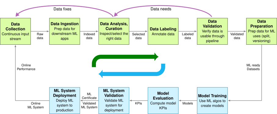](https://mlsysbook.ai/contents/core/workflow/03bbeaedbd5366f135a9b5e0ac5ecbb9aab154a3.svg "Figure 1: ML Lifecycle Stages: The prominent feedback arrows (shown as thick curved lines with bold colors) emphasize the iterative nature of machine learning development, where monitoring insights continuously inform data refinements, evaluation results trigger model improvements, and deployment experiences reshape data collection strategies. These visual feedback loops represent the primary drivers of the ML lifecycle, distinguishing it from linear development approaches where later stages rarely influence earlier phases.")
Figure 1: **ML Lifecycle Stages**: The prominent feedback arrows (shown as thick curved lines with bold colors) emphasize the iterative nature of machine learning development, where monitoring insights continuously inform data refinements, evaluation results trigger model improvements, and deployment experiences reshape data collection strategies. These visual feedback loops represent the primary drivers of the ML lifecycle, distinguishing it from linear development approaches where later stages rarely influence earlier phases.
This workflow framework serves as scaffolding for the technical chapters ahead. The data pipeline illustrated here receives comprehensive treatment in **[Chapter 6: Data Engineering](https://mlsysbook.ai/contents/core/data_engineering/data_engineering.html#sec-data-engineering)
**, which addresses how to ensure data quality and manage data throughout the ML lifecycle. Model training expands into **[Chapter 8: AI Training](https://mlsysbook.ai/contents/core/training/training.html#sec-ai-training)
**, covering how to efficiently train models at scale. The software frameworks that enable this iterative development process are detailed in **[Chapter 7: AI Frameworks](https://mlsysbook.ai/contents/core/frameworks/frameworks.html#sec-ai-frameworks)
**. Deployment and ongoing operations extend into **[Chapter 13: ML Operations](https://mlsysbook.ai/contents/core/ops/ops.html#sec-ml-operations)
**, addressing how systems maintain performance in production. This chapter establishes how these pieces interconnect before we explore each in depth—understanding the complete system makes the specialized components meaningful.
This chapter focuses on the conceptual stages of the ML lifecycle—the “what” and “why” of the development process. The operational implementation of this lifecycle through automation, tooling, and infrastructure—the “how”—is the domain of MLOps, which we will explore in detail in **[Chapter 13: ML Operations](https://mlsysbook.ai/contents/core/ops/ops.html#sec-ml-operations)
**. This distinction is crucial: the lifecycle provides the systematic framework for understanding ML development stages, while MLOps provides the operational practices for implementing these stages at scale. Understanding this lifecycle foundation makes the specialized MLOps tools and practices meaningful rather than appearing as disparate operational concerns.
**Self-Check: Question 1.2**
1. Which of the following best describes the role of feedback loops in the ML lifecycle?
1. They ensure that each stage of the lifecycle is completed before moving to the next.
2. They are used to validate the final model before deployment.
3. They allow for continuous improvement by informing earlier stages with insights from later stages.
4. They help in maintaining a linear development process.
2. Explain how systems thinking applies to the machine learning lifecycle and why it is important.
3. Order the following stages of the ML lifecycle from data collection to deployment: (1) Model Training, (2) Data Preparation, (3) Model Evaluation, (4) Data Collection, (5) ML System Deployment.
4. True or False: The ML lifecycle is a linear process where each stage is independent of the others.
[See Answers →](https://mlsysbook.ai/contents/core/workflow/workflow.html#quiz-answer-sec-ai-workflow-understanding-ml-lifecycle-8445)
ML vs Traditional Software Development
--------------------------------------
Machine learning requires specialized lifecycle approaches because ML development differs fundamentally from traditional software engineering. Traditional lifecycles consist of sequential phases: requirements gathering, system design, implementation, testing, and deployment ([Royce 1987](https://mlsysbook.ai/contents/core/workflow/workflow.html#ref-royce1970managing)
)[4](https://mlsysbook.ai/contents/core/workflow/workflow.html#fn4)
. Each phase produces specific artifacts that serve as inputs to subsequent phases. In financial software development, the requirements phase produces detailed specifications for transaction processing, security protocols, and regulatory compliance. These specifications translate directly into system behavior through explicit programming, contrasting sharply with the probabilistic nature of ML systems explored throughout **[Chapter 1: Introduction](https://mlsysbook.ai/contents/core/introduction/introduction.html#sec-introduction)
**.
Royce, W. W. 1987. “Managing the Development of Large Software Systems: Concepts and Techniques.” In _Proceedings of IEEE WESCON_, 26:328–39. IEEE. [http://dl.acm.org/citation.cfm?id=41801](http://dl.acm.org/citation.cfm?id=41801)
.
4 **Waterfall Model**: A sequential software development methodology introduced by Winston Royce in 1970, where development flows through distinct phases (requirements → design → implementation → testing → deployment) like water flowing down stairs. Each phase must be completed before the next begins, with formal documentation and approval gates. While criticized for inflexibility, waterfall dominated enterprise software development for decades and still suits projects with stable, well-understood requirements. The model’s linear approach contrasts starkly with ML development’s inherent uncertainty and need for experimentation.
5 **ML-Based Fraud Detection Evolution**: Traditional rule-based fraud systems had 60-80% accuracy and generated 10-40% false positives. Modern ML fraud detection achieves 85-95% accuracy with 1-5% false positive rates by analyzing hundreds of behavioral features ([Arsene, Dumitrache, and Mihu 2015](https://mlsysbook.ai/contents/core/workflow/workflow.html#ref-stripe2019machine)
). However, this improvement comes with new challenges: fraudsters adapt to ML patterns within 3-6 months, requiring continuous model retraining that rule-based systems never needed ([Arsene, Dumitrache, and Mihu 2015](https://mlsysbook.ai/contents/core/workflow/workflow.html#ref-stripe2019machine)
).
Machine learning systems require a fundamentally different approach. The deterministic nature of conventional software, where behavior is explicitly programmed, contrasts with the probabilistic nature of ML systems. Consider financial transaction processing: traditional systems follow predetermined rules (if account balance > transaction amount, then allow transaction), while ML-based fraud detection systems[5](https://mlsysbook.ai/contents/core/workflow/workflow.html#fn5)
learn to recognize suspicious patterns from historical transaction data. This shift from explicit programming to learned behavior reshapes the development lifecycle, altering how we approach system reliability and robustness as detailed in **[Chapter 16: Robust AI](https://mlsysbook.ai/contents/core/robust_ai/robust_ai.html#sec-robust-ai)
**.
These fundamental differences in system behavior introduce new dynamics that alter how lifecycle stages interact. These systems require ongoing refinement through continuous feedback loops that enable insights from deployment to inform earlier development phases. Machine learning systems are inherently dynamic and must adapt to changing data distributions and objectives through continuous deployment[6](https://mlsysbook.ai/contents/core/workflow/workflow.html#fn6)
practices.
6 **Continuous Deployment**: Software engineering practice where code changes are automatically deployed to production after passing automated tests, enabling multiple deployments per day instead of monthly releases. Popularized by companies like Netflix (2008) and Etsy (2009), continuous deployment reduces deployment risk through small, frequent changes rather than large, infrequent releases. However, ML systems require specialized continuous deployment because models need statistical validation, gradual rollouts with A/B testing, and rollback mechanisms based on performance metrics rather than just functional correctness.
7 **Data Versioning Challenges**: Unlike code, which changes through discrete edits, data can change gradually through drift, suddenly through schema changes, or subtly through quality degradation. Traditional version control systems like Git struggle with large datasets, leading to specialized tools like Git LFS and DVC.
These contrasts become clearer when we examine the specific differences across development lifecycle dimensions. The key distinctions are summarized in [Table 1](https://mlsysbook.ai/contents/core/workflow/workflow.html#tbl-sw-ml-cycles)
below. These differences reflect the core challenge of working with data as a first-class citizen in system design, something traditional software engineering methodologies were not designed to handle[7](https://mlsysbook.ai/contents/core/workflow/workflow.html#fn7)
.
Table 1: **Traditional vs ML Development**: Traditional software and machine learning systems diverge in their development processes due to the data-driven and iterative nature of ML. Machine learning lifecycles emphasize experimentation and evolving objectives, requiring feedback loops between stages, whereas traditional software follows a linear progression with predefined specifications.
| | | |
| --- | --- | --- |
| **Problem Definition** | Precise functional specifications are defined upfront. | Performance-driven objectives evolve as the problem space is explored. |
| **Development Process** | Linear progression of feature implementation. | Iterative experimentation with data, features and models. |
| **Testing and** | Deterministic, binary pass/fail | Statistical validation and metrics that |
| **Validation** | testing criteria. | involve uncertainty. |
| **Deployment** | Behavior remains static until explicitly updated. | Performance may change over time due to shifts in data distributions. |
| **Maintenance** | Maintenance involves modifying code to address bugs or add features. | Continuous monitoring, updating data pipelines, retraining models, and adapting to new data distributions. |
| **Feedback Loops** | Minimal; later stages rarely impact earlier phases. | Frequent; insights from deployment and monitoring often refine earlier stages like data preparation and model design. |
These six dimensions reveal a fundamental pattern: machine learning systems replace deterministic specifications with probabilistic optimization, static behavior with dynamic adaptation, and isolated development with continuous feedback. This shift explains why traditional project management approaches fail when applied to ML projects without modification.
Experimentation in machine learning differs fundamentally from testing in traditional software. In ML, experimentation constitutes the core development process itself, not simply bug detection. It involves systematically testing hypotheses about data sources, feature engineering approaches, model architectures, and hyperparameters to yield optimal performance. This represents a scientific process of discovery, not merely a quality assurance step. Traditional software testing verifies code behavior according to predetermined specifications, while ML experimentation explores uncertain spaces to discover optimal combinations producing the best empirical results.
These differences emphasize the need for robust ML lifecycle frameworks that accommodate iterative development, dynamic behavior, and data-driven decision-making. Understanding these distinctions enables examination of how ML projects unfold through their lifecycle stages, each presenting unique challenges that traditional software methodologies cannot adequately address.
This foundation enables exploration of the specific stages comprising the ML lifecycle and how they address these unique challenges.
**Self-Check: Question 1.3**
1. Which of the following best describes a key difference between traditional software development and machine learning development?
1. Traditional software development follows a linear progression with predefined specifications, whereas ML development involves iterative experimentation and evolving objectives.
2. ML development relies on deterministic specifications, while traditional development is probabilistic.
3. Traditional software development is iterative, while ML development is linear.
4. ML development does not require feedback loops, unlike traditional software development.
2. Explain why continuous feedback loops are crucial in the machine learning development lifecycle.
3. Order the following dimensions of development lifecycle differences between traditional software and ML systems: (1) Deployment, (2) Testing and Validation, (3) Feedback Loops.
[See Answers →](https://mlsysbook.ai/contents/core/workflow/workflow.html#quiz-answer-sec-ai-workflow-ml-vs-traditional-software-development-0f90)
Six Core Lifecycle Stages
-------------------------
AI systems require specialized development approaches. The specific stages that comprise the ML lifecycle provide this specialized framework. These stages operate as an integrated framework where each builds upon previous foundations while preparing for subsequent phases.
Moving from the detailed pipeline view in [Figure 1](https://mlsysbook.ai/contents/core/workflow/workflow.html#fig-ml-lifecycle)
, we now present a higher-level conceptual perspective. [Figure 2](https://mlsysbook.ai/contents/core/workflow/workflow.html#fig-lifecycle-overview)
consolidates these detailed pipelines into six major lifecycle stages, providing a simplified framework for understanding the overall progression of ML system development. This abstraction helps us reason about the broader phases without getting lost in pipeline-specific details. Where the earlier figure emphasized the parallel processing of data and models, this conceptual view emphasizes the sequential progression through major development phases—though as we’ll explore, these phases remain interconnected through continuous feedback.
[Figure 2](https://mlsysbook.ai/contents/core/workflow/workflow.html#fig-lifecycle-overview)
illustrates the six core stages that characterize successful AI system development: Problem Definition establishes objectives and constraints, Data Collection & Preparation encompasses the entire data pipeline, Model Development & Training covers model creation, Evaluation & Validation ensures quality, Deployment & Integration brings systems to production, and Monitoring & Maintenance ensures continued effectiveness. These stages operate through continuous feedback loops, with insights from later stages frequently informing refinements in earlier phases. This cyclical nature reflects the experimental and data-driven characteristics that distinguish ML development from conventional software engineering.
[](https://mlsysbook.ai/contents/core/workflow/9b58b3aa72de00d638019e0cdf45f488ecf3911f.svg "Figure 2: ML System Lifecycle: The continuous feedback loop (emphasized by the prominent return path from monitoring back to data collection) drives iterative development that defines successful machine learning systems. This cycle progresses through problem definition, data preparation, model building, evaluation, deployment, and ongoing monitoring, but the large feedback arrow illustrates how insights from later stages continuously inform and refine earlier phases, enabling adaptation to changing requirements and data distributions.")
Figure 2: **ML System Lifecycle**: The continuous feedback loop (emphasized by the prominent return path from monitoring back to data collection) drives iterative development that defines successful machine learning systems. This cycle progresses through problem definition, data preparation, model building, evaluation, deployment, and ongoing monitoring, but the large feedback arrow illustrates how insights from later stages continuously inform and refine earlier phases, enabling adaptation to changing requirements and data distributions.
The lifecycle begins with problem definition and requirements gathering, where teams clearly define the problem to be solved, establish measurable performance objectives, and identify key constraints. Precise problem definition ensures alignment between the system’s goals and the desired outcomes, setting the foundation for all subsequent work.
Building on this foundation, the next stage assembles the data resources needed to realize these objectives. Data collection and preparation includes gathering relevant data, cleaning it, and preparing it for model training. This process involves curating diverse datasets, ensuring high-quality labeling, and developing preprocessing pipelines to address variations in the data. The complexities of this stage are explored in **[Chapter 6: Data Engineering](https://mlsysbook.ai/contents/core/data_engineering/data_engineering.html#sec-data-engineering)
**.
With data resources in place, the development process creates models that can learn from these resources. Model development and training involves selecting appropriate algorithms, designing model architectures, and training models using the prepared data. Success depends on choosing techniques suited to the problem and iterating on the model design for optimal performance. Advanced training approaches and distributed training strategies are detailed in **[Chapter 8: AI Training](https://mlsysbook.ai/contents/core/training/training.html#sec-ai-training)
**, while the underlying architectures are covered in **[Chapter 4: DNN Architectures](https://mlsysbook.ai/contents/core/dnn_architectures/dnn_architectures.html#sec-dnn-architectures)
**.
Once models are trained, rigorous evaluation ensures they meet performance requirements before deployment. This evaluation and validation stage involves rigorously testing the model’s performance against predefined metrics and validating its behavior in different scenarios, ensuring the model is accurate, reliable, and robust in real-world conditions.
With validation complete, models transition from development environments to operational systems through careful deployment processes. Deployment and integration requires addressing practical challenges such as system compatibility, scalability, and operational constraints across different deployment contexts ranging from cloud to edge environments, as explored in **[Chapter 2: ML Systems](https://mlsysbook.ai/contents/core/ml_systems/ml_systems.html#sec-ml-systems)
**.
The final stage recognizes that deployed systems require ongoing oversight to maintain performance and adapt to changing conditions. This monitoring and maintenance stage focuses on continuously tracking the system’s performance in real-world environments and updating it as necessary. Effective monitoring ensures the system remains relevant and accurate over time, adapting to changes in data, requirements, or external conditions.
### Case Study: Diabetic Retinopathy Screening System
To ground these lifecycle principles in reality, we examine the development of diabetic retinopathy (DR) screening systems from initial research to widespread clinical deployment ([Gulshan et al. 2016](https://mlsysbook.ai/contents/core/workflow/workflow.html#ref-gulshan2016deep)
). Throughout this chapter, we use this case as a pedagogical vehicle to demonstrate how lifecycle stages interconnect in practice, showing how decisions in one phase influence subsequent stages.
_Note: While this narrative draws from documented experiences with diabetic retinopathy screening deployments, including Google’s work, we have adapted and synthesized details to illustrate common challenges encountered in healthcare AI systems. Our goal is educational—demonstrating lifecycle principles through a realistic example—rather than providing a documentary account of any specific project. The technical choices, constraints, and solutions presented represent typical patterns in medical AI development that illuminate broader systems thinking principles._
#### From Research Success to Clinical Reality
The DR screening challenge initially appeared straightforward: develop an AI system to analyze retinal images and detect signs of diabetic retinopathy with accuracy comparable to expert ophthalmologists. Initial research results achieved expert-level performance in controlled laboratory conditions. However, the journey from research success to clinical impact revealed AI lifecycle complexity, where technical excellence must integrate with operational realities, regulatory requirements, and real-world deployment constraints.
The scale of this medical challenge explains why AI-assisted screening became medically essential, not merely technically interesting. Diabetic retinopathy affects over 100 million people worldwide and represents a leading cause of preventable blindness[8](https://mlsysbook.ai/contents/core/workflow/workflow.html#fn8)
. [Figure 3](https://mlsysbook.ai/contents/core/workflow/workflow.html#fig-eye-dr)
shows the clinical challenge: distinguishing healthy retinas from those showing early signs of retinopathy, such as the characteristic hemorrhages visible as dark red spots. While this appears to be a straightforward image classification problem, the path from laboratory success to clinical deployment illustrates every aspect of the AI lifecycle complexity.
8 **Diabetic Retinopathy Global Impact**: Affects approximately 93-103 million people worldwide, with 22.27% to 35% of diabetic patients developing some form of retinopathy ([Steinmetz et al. 2024](https://mlsysbook.ai/contents/core/workflow/workflow.html#ref-who2019classification)
). In developing countries, up to 90% of vision loss from diabetes is preventable with early detection, but access to ophthalmologists remains severely limited: rural areas in India have approximately one ophthalmologist per 100,000-120,000 people, compared to the WHO recommendation of 1 per 20,000 ([Steinmetz et al. 2024](https://mlsysbook.ai/contents/core/workflow/workflow.html#ref-who2019classification)
). This stark disparity makes AI-assisted screening not just convenient but potentially life-changing for millions ([Rajkomar, Dean, and Kohane 2019](https://mlsysbook.ai/contents/core/workflow/workflow.html#ref-rajkomar2019machine)
).
Steinmetz, Jaimie D, Katrin Maria Seeher, Nicoline Schiess, Emma Nichols, Bochen Cao, Chiara Servili, Vanessa Cavallera, et al. 2024. “Global, Regional, and National Burden of Disorders Affecting the Nervous System, 1990–2021: A Systematic Analysis for the Global Burden of Disease Study 2021.” _The Lancet Neurology_ 23 (4): 344–81. [https://doi.org/10.1016/s1474-4422(24)00038-3](https://doi.org/10.1016/s1474-4422(24)00038-3)
.
[](https://mlsysbook.ai/contents/core/workflow/images/png/eye-dr.png "Figure 3: Retinal Hemorrhages: Diabetic retinopathy causes visible hemorrhages in retinal images, providing a key visual indicator for model training and evaluation in medical image analysis. these images represent the input data used to develop algorithms that automatically detect and classify retinal diseases, ultimately assisting in early diagnosis and treatment. Source: Google.")
Figure 3: **Retinal Hemorrhages**: Diabetic retinopathy causes visible hemorrhages in retinal images, providing a key visual indicator for model training and evaluation in medical image analysis. these images represent the input data used to develop algorithms that automatically detect and classify retinal diseases, ultimately assisting in early diagnosis and treatment. Source: Google.
#### Systems Engineering Lessons
DR system development illustrates fundamental AI systems principles across lifecycle stages. Challenges with data quality lead to innovations in distributed data validation. Infrastructure constraints in rural clinics drive breakthroughs in edge computing[9](https://mlsysbook.ai/contents/core/workflow/workflow.html#fn9)
optimization. Integration with clinical workflows reveals the importance of human-AI collaboration design. These experiences demonstrate that building robust AI systems requires more than accurate models; success demands systematic engineering approaches that address real-world deployment complexity.
9 **Edge Computing**: Distributed computing paradigm that processes data near the source rather than in centralized cloud data centers, reducing latency from 50-500ms (cloud) to 5-50ms (edge) depending on the application. Originally developed for CDNs (1990s), edge computing became essential for ML when real-time applications like autonomous vehicles and medical devices required sub-20ms response times that cloud computing couldn’t achieve ([Shi et al. 2016](https://mlsysbook.ai/contents/core/workflow/workflow.html#ref-shi2016edge)
). The edge AI market grew from approximately $1.12B in 2018 to $8.2B in 2023, driven by IoT devices generating an estimated 73-80 zettabytes of data annually by 2025 that cannot be efficiently transmitted to cloud servers.
Shi, Weisong, Jie Cao, Quan Zhang, Youhuizi Li, and Lanyu Xu. 2016. “Edge Computing: Vision and Challenges.” _IEEE Internet of Things Journal_ 3 (5): 637–46. [https://doi.org/10.1109/jiot.2016.2579198](https://doi.org/10.1109/jiot.2016.2579198)
.
10 **Healthcare AI Deployment Reality**: Studies show that 75-80% of healthcare AI projects never reach clinical deployment ([Chen and Asch 2017](https://mlsysbook.ai/contents/core/workflow/workflow.html#ref-chen2019machine)
), with the majority failing not due to algorithmic issues but due to integration challenges, regulatory hurdles, and workflow disruption. The “AI chasm” between research success and clinical adoption is particularly wide in healthcare: while medical AI papers show 95%+ accuracy rates, real-world implementation studies report significant performance drops due to data drift, equipment variations, and user acceptance issues ([Kelly et al. 2019](https://mlsysbook.ai/contents/core/workflow/workflow.html#ref-kelly2019key)
).
Chen, Jonathan H., and Steven M. Asch. 2017. “Machine Learning and Prediction in Medicine — Beyond the Peak of Inflated Expectations.” _New England Journal of Medicine_ 376 (26): 2507–9. [https://doi.org/10.1056/nejmp1702071](https://doi.org/10.1056/nejmp1702071)
.
Kelly, Christopher J., Alan Karthikesalingam, Mustafa Suleyman, Greg Corrado, and Dominic King. 2019. “Key Challenges for Delivering Clinical Impact with Artificial Intelligence.” _BMC Medicine_ 17 (1): 1–9. [https://doi.org/10.1186/s12916-019-1426-2](https://doi.org/10.1186/s12916-019-1426-2)
.
This comprehensive journey through real-world deployment challenges reflects broader patterns in healthcare AI development. Throughout each lifecycle stage, the DR case study demonstrates how decisions made in early phases influence later stages, how feedback loops drive continuous improvement, and how emergent system behaviors require holistic solutions. These deployment challenges reflect broader issues in healthcare AI[10](https://mlsysbook.ai/contents/core/workflow/workflow.html#fn10)
that affect most real-world medical ML applications.
This narrative thread demonstrates how the AI lifecycle’s integrated nature requires systems thinking from the beginning. The DR case shows that sustainable AI systems emerge from understanding and designing for complex interactions between all lifecycle stages, rather than from optimizing individual components in isolation.
With this framework and case study established, examination of each lifecycle stage begins with problem definition.
**Self-Check: Question 1.4**
1. Which of the following best describes the purpose of the ‘Problem Definition’ stage in the ML lifecycle?
1. To define objectives and constraints for the ML system.
2. To gather and clean data for model training.
3. To deploy the model into production environments.
4. To monitor the system’s performance post-deployment.
2. Order the following ML lifecycle stages from start to finish: (1) Deployment & Integration, (2) Model Development & Training, (3) Data Collection & Preparation, (4) Monitoring & Maintenance.
3. How does the feedback loop in the ML lifecycle contribute to the system’s adaptability and improvement?
4. In the context of the DR screening system, which lifecycle stage likely involves ensuring model performance in real-world conditions?
1. Problem Definition
2. Data Collection & Preparation
3. Evaluation & Validation
4. Monitoring & Maintenance
[See Answers →](https://mlsysbook.ai/contents/core/workflow/workflow.html#quiz-answer-sec-ai-workflow-six-core-lifecycle-stages-fab9)
Problem Definition Stage
------------------------
Machine learning system development begins with a challenge distinct from traditional software development: defining not just what the system should do, but how it should learn to do it. Conventional software requirements translate directly into implementation rules, while ML systems require teams to consider how the system will learn from data while operating within real-world constraints[11](https://mlsysbook.ai/contents/core/workflow/workflow.html#fn11)
. This first stage shown in [Figure 2](https://mlsysbook.ai/contents/core/workflow/workflow.html#fig-lifecycle-overview)
lays the foundation for all subsequent phases in the ML lifecycle.
11 **ML vs. Traditional Problem Definition**: Traditional software problems are defined by deterministic specifications (“if input X, then output Y”), but ML problems are defined by examples and desired behaviors. This shift means that Studies suggest 60-80% of ML projects fail, with many failures occurring during problem formulation and requirements phases, compared to lower failure rates in traditional software projects ([Maor 1987](https://mlsysbook.ai/contents/core/workflow/workflow.html#ref-standish2020chaos)
). The challenge lies in translating business objectives into learning objectives—something that didn’t exist in software engineering until the rise of data-driven systems in the 2000s ([Amershi et al. 2019](https://mlsysbook.ai/contents/core/workflow/workflow.html#ref-amershi2019software)
).
Maor, Eli. 1987. “CHAOS 2020: Beyond Infinity.” In _To Infinity and Beyond_, 60–65. Birkhäuser Boston. [https://doi.org/10.1007/978-1-4612-5394-5\\\_10](https://doi.org/10.1007/978-1-4612-5394-5/_10)
.
Amershi, Saleema, Andrew Begel, Christian Bird, Robert DeLine, Harald Gall, Ece Kamar, Nachiappan Nagappan, Besmira Nushi, and Thomas Zimmermann. 2019. “Software Engineering for Machine Learning: A Case Study.” In _2019 IEEE/ACM 41st International Conference on Software Engineering: Software Engineering in Practice (ICSE-SEIP)_, 291–300. IEEE. [https://doi.org/10.1109/icse-seip.2019.00042](https://doi.org/10.1109/icse-seip.2019.00042)
.
The DR screening example illustrates how this complexity manifests in practice. A diabetic retinopathy screening system’s problem definition reveals complexity beneath an apparently straightforward medical imaging task. What initially appeared straightforward computer vision actually required defining multiple interconnected objectives that shaped every subsequent lifecycle stage.
Development teams balance competing constraints in such systems: diagnostic accuracy for patient safety, computational efficiency for rural clinic hardware, workflow integration for clinical adoption, regulatory compliance for medical device approval, and cost-effectiveness for sustainable deployment. Each constraint influences the others, creating a complex optimization problem that traditional software development approaches cannot address. This multi-dimensional problem definition drives data collection strategies, model architecture choices, and deployment infrastructure decisions throughout the project lifecycle.
### Balancing Competing Constraints
Problem definition decisions cascade through system design. Requirements analysis in a DR screening system evolves from initial focus on diagnostic accuracy metrics to encompass deployment environment constraints and opportunities.
Achieving 90%+ sensitivity for detecting referable diabetic retinopathy prevents vision loss, while maintaining 80%+ specificity avoids overwhelming referral systems with false positives. These metrics must be achieved across diverse patient populations, camera equipment, and image quality conditions typical in resource-limited settings.
Rural clinic deployments impose strict constraints reflecting edge deployment challenges from **[Chapter 2: ML Systems](https://mlsysbook.ai/contents/core/ml_systems/ml_systems.html#sec-ml-systems)
**: models must run on devices with limited computational power, operate reliably with intermittent internet connectivity, and produce results within clinical workflow timeframes. These systems require operation by healthcare workers with minimal technical training.
Medical device regulations require extensive validation, audit trails, and performance monitoring capabilities that influence data collection, model development, and deployment strategies.
These interconnected requirements demonstrate how problem definition in ML systems requires understanding the complete ecosystem in which the system will operate. Early recognition of these constraints enables teams to make architecture decisions crucial for successful deployment, rather than discovering limitations after significant development investment.
### Collaborative Problem Definition Process
Establishing clear and actionable problem definitions involves a systematic workflow that bridges technical, operational, and user considerations. The process begins with identifying the core objective of the system: what tasks it must perform and what constraints it must satisfy. Teams collaborate with stakeholders to gather domain knowledge, outline requirements, and anticipate challenges that may arise in real-world deployment.
In a DR-type project, this phase involves close collaboration with clinicians to determine the diagnostic needs of rural clinics. Key decisions, such as balancing model complexity with hardware limitations and ensuring interpretability for healthcare providers, emerge during this phase. The approach must account for regulatory considerations, such as patient privacy and compliance with healthcare standards. This collaborative process ensures that the problem definition aligns with both technical feasibility and clinical relevance.
### Adapting Definitions for Scale
As ML systems scale, their problem definitions must adapt to new operational challenges[12](https://mlsysbook.ai/contents/core/workflow/workflow.html#fn12)
. A DR-type system might initially focus on a limited number of clinics with consistent imaging setups. However, as such a system expands to include clinics with varying equipment, staff expertise, and patient demographics[13](https://mlsysbook.ai/contents/core/workflow/workflow.html#fn13)
, the original problem definition requires adjustments to accommodate these variations.
12 **ML System Scaling Complexity**: Scaling ML systems is exponentially more complex than traditional software due to data heterogeneity, model drift, and infrastructure requirements. Studies show that ML systems typically require 5-10x more monitoring infrastructure than traditional applications ([Paleyes, Urma, and Lawrence 2022](https://mlsysbook.ai/contents/core/workflow/workflow.html#ref-paleyes2022challenges)
), with companies like Uber running 1,000+ model quality checks daily across their ML platform ([Hermann and Del Balso 2017](https://mlsysbook.ai/contents/core/workflow/workflow.html#ref-uber2017michelangelo)
). The “scaling wall” typically hits at 100+ models in production, where manual processes break down and teams need specialized MLOps platforms—explaining why the ML platform market grew from approximately $1.5B in 2019 to $15.5B in 2023, with MLOps tools representing a significant subset ([Kreuzberger, Kühl, and Hirschl 2023](https://mlsysbook.ai/contents/core/workflow/workflow.html#ref-kreuzberger2023machine)
).
Kreuzberger, Dominik, Niklas Kühl, and Sebastian Hirschl. 2023. “Machine Learning Operations (MLOps): Overview, Definition, and Architecture.” _IEEE Access_ 11: 31866–79. [https://doi.org/10.1109/access.2023.3262138](https://doi.org/10.1109/access.2023.3262138)
.
13 **Algorithmic Fairness in Healthcare**: Medical AI systems show significant performance disparities across demographic groups—dermatology AI systems show significant performance disparities, with some studies reporting 10-36% worse accuracy on darker skin tones depending on the specific condition and dataset ([Chin-Purcell and Chambers 2021](https://mlsysbook.ai/contents/core/workflow/workflow.html#ref-larson2017gender)
), while diabetic retinopathy models trained primarily on European populations show 15-25% accuracy drops for Asian and African populations ([Gulshan et al. 2016](https://mlsysbook.ai/contents/core/workflow/workflow.html#ref-gulshan2016deep)
). The FDA’s 2021 Action Plan for AI/ML-based medical devices now requires demographic performance reporting ([Food and Administration 2021](https://mlsysbook.ai/contents/core/workflow/workflow.html#ref-fda2021artificial)
), and companies like Google Health spend 20-30% of development resources on fairness testing and bias mitigation across racial, gender, and socioeconomic groups ([Rajkomar, Dean, and Kohane 2019](https://mlsysbook.ai/contents/core/workflow/workflow.html#ref-rajkomar2019machine)
).
Chin-Purcell, Lia, and America Chambers. 2021. “Investigating Accuracy Disparities for Gender Classification Using Convolutional Neural Networks.” In _2021 IEEE International Symposium on Technology and Society (ISTAS)_, 81:1–7. IEEE. [https://doi.org/10.1109/istas52410.2021.9629153](https://doi.org/10.1109/istas52410.2021.9629153)
.
Gulshan, Varun, Lily Peng, Marc Coram, Martin C. Stumpe, Derek Wu, Arunachalam Narayanaswamy, Subhashini Venugopalan, et al. 2016. “Development and Validation of a Deep Learning Algorithm for Detection of Diabetic Retinopathy in Retinal Fundus Photographs.” _JAMA_ 316 (22): 2402. [https://doi.org/10.1001/jama.2016.17216](https://doi.org/10.1001/jama.2016.17216)
.
Food, U. S., and Drug Administration. 2021. “Artificial Intelligence/Machine Learning (AI/ML)-Based Software as a Medical Device (SaMD) Action Plan.” U.S. Department of Health; Human Services. [https://www.fda.gov/media/145022/download](https://www.fda.gov/media/145022/download)
.
Rajkomar, Alvin, Jeffrey Dean, and Isaac Kohane. 2019. “Machine Learning in Medicine.” _New England Journal of Medicine_ 380 (14): 1347–58. [https://doi.org/10.1056/nejmra1814259](https://doi.org/10.1056/nejmra1814259)
.
Scaling also introduces data challenges. Larger datasets may include more diverse edge cases, which can expose weaknesses in the initial model design. Expanding deployment to new regions introduces variations in imaging equipment and patient populations that require further system tuning. Defining a problem that accommodates such diversity from the outset ensures the system can handle future expansion without requiring a complete redesign.
In our DR example, the problem definition process shapes data collection strategy. Requirements for multi-population validation drive the need for diverse training data, while edge deployment constraints influence data preprocessing approaches. Regulatory compliance needs determine annotation protocols and quality assurance standards. These interconnected requirements demonstrate how effective problem definition anticipates constraints that will emerge in subsequent lifecycle stages, establishing a foundation for integrated system development rather than sequential, isolated optimization.
With clear problem definition established, the development process transitions to assembling the data resources needed to achieve these objectives.
**Self-Check: Question 1.5**
1. How does problem definition in machine learning differ from traditional software development?
1. It involves defining how the system should learn from data.
2. It focuses solely on deterministic specifications.
3. It requires no consideration of real-world constraints.
4. It is based on fixed input-output rules.
2. Why is it crucial to align problem definition with real-world constraints in ML system development?
3. In ML systems, the process of translating business objectives into learning objectives is known as \_\_\_\_.
4. Which of the following best describes a key challenge in scaling ML systems?
1. Data homogeneity across all environments.
2. Consistent model performance without additional tuning.
3. Data heterogeneity and infrastructure requirements.
4. Simplified monitoring infrastructure compared to traditional applications.
5. In a production system, how might problem definition influence the choice of deployment infrastructure?
[See Answers →](https://mlsysbook.ai/contents/core/workflow/workflow.html#quiz-answer-sec-ai-workflow-problem-definition-stage-3e18)
Data Collection & Preparation Stage
-----------------------------------
Data collection and preparation represent the second stage in the ML lifecycle ([Figure 2](https://mlsysbook.ai/contents/core/workflow/workflow.html#fig-lifecycle-overview)
), where raw data is gathered, processed, and prepared for model development. This stage presents unique challenges extending beyond gathering sufficient training examples[14](https://mlsysbook.ai/contents/core/workflow/workflow.html#fn14)
. These challenges form the core focus of **[Chapter 6: Data Engineering](https://mlsysbook.ai/contents/core/data_engineering/data_engineering.html#sec-data-engineering)
**. For medical AI systems like DR screening, data collection must balance statistical rigor with operational feasibility while meeting the highest standards for diagnostic accuracy.
14 **The 80/20 Rule in ML**: Data scientists typically spend 60-80% of their time on data collection, cleaning, and preparation, with the remainder on modeling and analysis. This ratio, first documented by CrowdFlower ([CrowdFlower, n.d.](https://mlsysbook.ai/contents/core/workflow/workflow.html#ref-crowdflower2016data)
) in 2016, remains consistent across industries despite advances in automated tools. The “data preparation tax” includes handling missing values (present in 90% of real-world datasets), resolving inconsistencies (affecting 60% of data fields), and ensuring legal compliance (requiring 15+ different consent mechanisms for EU data). This explains why successful ML teams invest heavily in data engineering capabilities from day one.
CrowdFlower. n.d. “Supplemental Information 1: Source Code for Analysis in Matlab, Correlation Matrix, XML Code for Crowdflower Survey.” _CrowdFlower Inc_. PeerJ. [https://doi.org/10.7287/peerj.preprints.1069/supp-1](https://doi.org/10.7287/peerj.preprints.1069/supp-1)
.
Problem definition decisions shape data requirements in the DR example. The multi-dimensional success criteria established (accuracy across diverse populations, hardware efficiency, and regulatory compliance) demand a data collection strategy that goes beyond typical computer vision datasets.
Building this foundation in such a system might require assembling a development dataset of 128,000 retinal fundus photographs, each reviewed by 3-7 expert ophthalmologists from a panel of 54 specialists[15](https://mlsysbook.ai/contents/core/workflow/workflow.html#fn15)
. This expert consensus approach addresses the inherent subjectivity in medical diagnosis while establishing ground truth labels that can withstand regulatory scrutiny. The annotation process captures clinically relevant features like microaneurysms, hemorrhages, and hard exudates across the spectrum of disease severity.
15 **Medical Data Annotation Costs**: Expert medical annotation is extraordinarily expensive: ophthalmologists charge $200-500 per hour, meaning the DR dataset’s annotation cost exceeded $2.7 million in expert time alone. This represents one of the highest annotation costs per sample in ML history, driving interest in active learning and synthetic data generation.
High-resolution retinal scans typically generate files ranging from 10-120 megabytes depending on resolution and compression, creating substantial infrastructure challenges. A typical clinic processing 50 patients daily generates 5-15 GB of imaging data per week depending on image quality and compression, quickly exceeding the capacity of rural internet connections (often limited to 2-10 Mbps upload speeds). This data volume constraint forces architectural decisions toward edge-computing solutions rather than cloud-based processing.
### Bridging Laboratory and Real-World Data
Transitioning from laboratory-quality training data to real-world deployment reveals fundamental gaps when such a system moves to rural clinic settings.
When deployment begins in rural clinics across regions like Thailand and India, real-world data differs dramatically from carefully curated training sets. Images come from diverse camera equipment operated by staff with varying expertise levels, often under suboptimal lighting conditions and with inconsistent patient positioning. These variations threaten model performance and reveal the need for robust preprocessing and quality assurance systems.
This data volume constraint drives a fundamental architectural decision between the deployment paradigms discussed in **[Chapter 2: ML Systems](https://mlsysbook.ai/contents/core/ml_systems/ml_systems.html#sec-ml-systems)
**: edge computing deployment rather than cloud-based inference. Local preprocessing reduces bandwidth requirements by 95% (from 15 GB to 750 MB weekly transmission) but requires 10x more local computational resources, shaping both model optimization strategies and deployment hardware requirements using specialized edge devices like NVIDIA Jetson[16](https://mlsysbook.ai/contents/core/workflow/workflow.html#fn16)
.
16 **NVIDIA Jetson**: Series of embedded computing boards designed for AI edge computing, featuring GPU acceleration in power-efficient form factors (5-30 watts vs. 250+ watts for desktop GPUs). First released in 2014, Jetson modules enable real-time AI inference on devices like autonomous drones, medical equipment, and industrial robots. Popular models include Jetson Nano ($99, 472 GFLOPS), Jetson AGX Xavier ($699, 32 TOPS), and Jetson AGX Orin ($1,699, 275 TOPS), making high-performance AI accessible for edge deployment scenarios where cloud connectivity is unreliable or latency-critical.
A typical solution architecture emerges from data collection constraints: NVIDIA Jetson edge devices (2-32GB RAM, 64-2048 CUDA cores depending on model) for local inference, clinic aggregation servers (8-core CPUs, 32GB RAM) for data management, and cloud training infrastructure using 32-GPU clusters for weekly model updates. This distributed approach achieves sub-80ms inference latency with 94% uptime across deployments spanning 200+ clinic locations.
Patient privacy regulations require federated learning architecture, enabling model training without centralizing sensitive patient data. This approach adds complexity to both data collection workflows and model training infrastructure, but proves essential for regulatory approval and clinical adoption.
These experiences illustrate the constraint propagation principles we established earlier: lifecycle decisions in data collection create constraints and opportunities that propagate through the entire system development process, shaping everything from infrastructure design to model architecture.
### Data Infrastructure for Distributed Deployment
Understanding how data characteristics and deployment constraints drive architectural decisions becomes critical at scale. Each retinal image follows a complex journey: capture on clinic cameras, local storage and initial processing, quality validation, secure transmission to central systems, and integration with training datasets.
Different data access patterns demand different storage solutions. Teams typically implement tiered approaches balancing cost, performance, and availability: frequently accessed training data requires high-speed storage for rapid model iteration, while historical datasets can tolerate slower access times in exchange for cost efficiency. Intelligent caching systems optimize data access based on usage patterns, ensuring that relevant data remains readily available.
Rural clinic deployments face significant connectivity constraints, requiring flexible data transmission strategies. Real-time transmission works well for clinics with reliable internet, while store-and-forward systems enable operation in areas with intermittent connectivity. This adaptive approach ensures consistent system operation regardless of local infrastructure limitations.
Infrastructure design must anticipate growth from pilot deployments to hundreds of clinics. The architecture accommodates varying data volumes, different hardware configurations, and diverse operational requirements while maintaining data consistency and system reliability. This scalability foundation proves essential as systems expand to new regions.
### Managing Data at Scale
Applying systems thinking to scale, data collection challenges grow exponentially as ML systems expand. In our DR example, scaling from initial clinics to a broader network introduces emergent complexity: significant variability in equipment, workflows, and operating conditions. Each clinic effectively becomes an independent data node[17](https://mlsysbook.ai/contents/core/workflow/workflow.html#fn17)
, yet the system needs to ensure consistent performance across all locations. Following the collaborative coordination patterns established earlier, teams implement specialized orchestration with shared artifact repositories, versioned APIs, and automated testing pipelines that enable efficient management of large clinic networks.
17 **Federated Learning Architecture**: Federated learning ([McMahan et al. 2017](https://mlsysbook.ai/contents/core/workflow/workflow.html#ref-mcmahan2017communication)
), introduced by Google in 2016 for mobile keyboards, enables training across distributed data sources without centralizing data. Healthcare applications are particularly suited for federated learning due to privacy regulations: studies show federated medical models achieve 85-95% of centralized model accuracy while keeping data local. However, federated learning introduces new challenges: communication costs increase 100-1000x per training iteration, and statistical heterogeneity across sites can cause model convergence issues that centralized training doesn’t face.
McMahan, Brendan, Eider Moore, Daniel Ramage, Seth Hampson, and Blaise Agüera y Arcas. 2017. “Communication-Efficient Learning of Deep Networks from Decentralized Data.” In _Artificial Intelligence and Statistics_, 1273–82. PMLR. [http://proceedings.mlr.press/v54/mcmahan17a.html](http://proceedings.mlr.press/v54/mcmahan17a.html)
.
Scaling such systems to additional clinics also brings increasing data volumes, as higher-resolution imaging devices become standard, generating larger and more detailed images. These advances amplify the demands on storage and processing infrastructure, requiring optimizations to maintain efficiency without compromising quality. Differences in patient demographics, clinic workflows, and connectivity patterns further underscore the need for robust design to handle these variations gracefully.
Scaling challenges highlight how decisions made during the data collection phase ripple through the lifecycle, impacting subsequent stages like model development, deployment, and monitoring. For instance, accommodating higher-resolution data during collection directly influences computational requirements for training and inference, emphasizing the need for lifecycle thinking even at this early stage.
### Quality Assurance and Validation
Quality assurance is an integral part of the data collection process, ensuring that data meets the requirements for downstream stages. In our DR example, automated checks at the point of collection flag issues like poor focus or incorrect framing, allowing clinic staff to address problems immediately. These proactive measures ensure that low-quality data is not propagated through the pipeline.
Validation systems extend these efforts by verifying not just image quality but also proper labeling, patient association, and compliance with privacy regulations. Operating at both local and centralized levels, these systems ensure data reliability and robustness, safeguarding the integrity of the entire ML pipeline.
The data collection experiences in such systems directly inform model development approaches. The infrastructure constraints discovered during data collection (limited bandwidth, diverse hardware, intermittent connectivity) establish requirements for model efficiency that drive architectural decisions. The distributed federated learning approach required by privacy constraints influences training pipeline design. The quality variations observed across different clinic environments shape validation strategies and robustness requirements. This coupling between data collection insights and model development strategies exemplifies how integrated lifecycle planning trumps sequential stage optimization.
[Figure 4](https://mlsysbook.ai/contents/core/workflow/workflow.html#fig-ml-lifecycle-feedback)
illustrates these critical feedback loops that enable continuous system improvement. The foundation established during data collection both enables and constrains the technical approaches available for creating effective models—a dynamic that becomes apparent as we now transition to model development.
[](https://mlsysbook.ai/contents/core/workflow/5d4c6dbc2d5c776a4c56979510d7852864221bd3.svg "Figure 4: ML Lifecycle Dependencies: Iterative feedback loops connect data collection, preparation, model training, evaluation, and monitoring, emphasizing that each stage informs and influences subsequent stages in a continuous process. Effective machine learning system development requires acknowledging these dependencies to refine data, retrain models, and maintain performance over time.")
Figure 4: **ML Lifecycle Dependencies**: Iterative feedback loops connect data collection, preparation, model training, evaluation, and monitoring, emphasizing that each stage informs and influences subsequent stages in a continuous process. Effective machine learning system development requires acknowledging these dependencies to refine data, retrain models, and maintain performance over time.
**Self-Check: Question 1.6**
1. Which of the following best describes a major challenge in data collection for medical AI systems like diabetic retinopathy screening?
1. Ensuring high-resolution images are captured consistently.
2. Reducing the cost of expert annotation.
3. Balancing statistical rigor with operational feasibility.
4. Maximizing the number of images collected daily.
2. How does the data volume constraint in rural clinics influence architectural decisions in ML systems?
3. Order the following steps involved in the data collection process for a medical AI system: (1) Initial processing and storage, (2) Data capture, (3) Quality validation, (4) Secure transmission.
4. What is a key reason for using federated learning in the data collection strategy for medical AI systems?
1. To improve model accuracy by centralizing data.
2. To comply with patient privacy regulations.
3. To reduce the cost of data annotation.
4. To increase the speed of data processing.
[See Answers →](https://mlsysbook.ai/contents/core/workflow/workflow.html#quiz-answer-sec-ai-workflow-data-collection-preparation-stage-a0aa)
Model Development & Training Stage
----------------------------------
Model development and training (the third stage in [Figure 2](https://mlsysbook.ai/contents/core/workflow/workflow.html#fig-lifecycle-overview)
) form the core of machine learning systems, yet this stage presents unique challenges extending beyond selecting algorithms and tuning hyperparameters[18](https://mlsysbook.ai/contents/core/workflow/workflow.html#fn18)
. The training methodologies, infrastructure requirements, and distributed training strategies are covered in **[Chapter 8: AI Training](https://mlsysbook.ai/contents/core/training/training.html#sec-ai-training)
**. In high-stakes domains like healthcare, every design decision impacts clinical outcomes, making the integration of technical performance with operational constraints critical.
18 **Hyperparameter Optimization Complexity**: Modern deep learning models have 10-100+ hyperparameters (learning rate, batch size, architecture choices), creating search spaces with 10^20+ possible combinations. AutoML platforms like Google’s AutoML and H2O spend $10,000-100,000 in compute costs to find optimal configurations for complex models. Random search (2012) surprisingly outperforms grid search, while Bayesian optimization (2010s) and population-based training (2017) represent current state-of-the-art, reducing tuning time by 10-100x but still requiring substantial computational resources that didn’t exist in traditional software development.
Early lifecycle decisions cascade through model development in our DR example. The problem definition requirements established (expert-level accuracy combined with edge device compatibility) create an optimization challenge that demands innovative approaches to both model architecture and training strategies.
**Definition:** Transfer Learning
**_Transfer Learning_** is the technique of adapting models _pretrained_ on large-scale datasets to new tasks, dramatically reducing _training time_ and _data requirements_ by leveraging learned representations.
Using transfer learning from ImageNet[19](https://mlsysbook.ai/contents/core/workflow/workflow.html#fn19)
combined with a meticulously labeled dataset of 128,000 images, developers in such projects achieve F-scores[20](https://mlsysbook.ai/contents/core/workflow/workflow.html#fn20)
of 0.91-0.95, comparable to or exceeding ophthalmologist performance in controlled settings. This result validates approaches that combine large-scale pre-training with domain-specific fine-tuning—a training strategy leveraging the gradient-based optimization principles from **[Chapter 3: Deep Learning Primer](https://mlsysbook.ai/contents/core/dl_primer/dl_primer.html#sec-dl-primer)
** to adapt pre-trained convolutional architectures from **[Chapter 4: DNN Architectures](https://mlsysbook.ai/contents/core/dnn_architectures/dnn_architectures.html#sec-dnn-architectures)
** for medical imaging.
19 **Transfer Learning**: A technique where models pre-trained on large datasets (like ImageNet’s 14 million images) are adapted for specific tasks, dramatically reducing training time and data requirements ([Krizhevsky, Sutskever, and Hinton 2017](https://mlsysbook.ai/contents/core/workflow/workflow.html#ref-krizhevsky2012imagenet)
; [Deng et al. 2009](https://mlsysbook.ai/contents/core/workflow/workflow.html#ref-deng2009imagenet)
). Introduced by Yann LeCun’s team in the 1990s and popularized by the 2014 ImageNet competition, transfer learning became the foundation for most practical computer vision applications. Instead of training from scratch, practitioners can achieve expert-level performance with thousands rather than millions of training examples.
Krizhevsky, Alex, Ilya Sutskever, and Geoffrey E. Hinton. 2017. “ImageNet Classification with Deep Convolutional Neural Networks.” _Communications of the ACM_ 60 (6): 84–90. [https://doi.org/10.1145/3065386](https://doi.org/10.1145/3065386)
.
Deng, Jia, Wei Dong, Richard Socher, Li-Jia Li, Kai Li, and Li Fei-Fei. 2009. “ImageNet: A Large-Scale Hierarchical Image Database.” In _2009 IEEE Conference on Computer Vision and Pattern Recognition_, 248–55. IEEE; IEEE. [https://doi.org/10.1109/cvpr.2009.5206848](https://doi.org/10.1109/cvpr.2009.5206848)
.
20 **F-Score (F1 Score)**: The harmonic mean of precision and recall, calculated as 2 × (precision × recall) / (precision + recall), providing a single metric that balances both measures. Values range from 0 (worst) to 1 (perfect). Introduced in information retrieval (1979), F-score became essential for ML evaluation because accuracy alone can be misleading with imbalanced datasets—a model predicting “no disease” for all patients might achieve 95% accuracy in a population where only 5% have the condition, but would have an F-score near 0, revealing its clinical uselessness.
21 **Ensemble Learning**: A technique that combines predictions from multiple models to achieve better performance than any individual model. Common methods include bagging (training multiple models on different data subsets), boosting (sequentially training models to correct previous errors), and stacking (using a meta-model to combine base model predictions). Netflix’s recommendation system uses ensembles of 100+ algorithms, while winning entries in ML competitions typically ensemble 10-50 models. However, ensembles trade inference speed and memory usage for accuracy—a critical constraint in edge deployment scenarios.
Achieving high accuracy is only the first challenge. Data collection insights about edge deployment constraints impose strict efficiency requirements: models must operate under 98MB in size, achieve sub-50ms inference latency, and consume under 400MB RAM during operation. The initial research model (a 2.1GB ensemble[21](https://mlsysbook.ai/contents/core/workflow/workflow.html#fn21)
achieving 95.2% accuracy) violates all deployment constraints, requiring systematic optimization to reach a final 96MB model maintaining 94.8% accuracy while meeting all operational requirements.
These constraints drive architectural innovations including model optimization techniques for size reduction, inference acceleration, and efficient deployment scenarios—balancing the computational demands of deep convolutional networks from **[Chapter 4: DNN Architectures](https://mlsysbook.ai/contents/core/dnn_architectures/dnn_architectures.html#sec-dnn-architectures)
** with the resource limitations of edge devices detailed in **[Chapter 2: ML Systems](https://mlsysbook.ai/contents/core/ml_systems/ml_systems.html#sec-ml-systems)
**.
Following the iterative development framework established, the model development process requires continuous iteration between accuracy optimization and efficiency optimization. Each architectural decision (from the number of convolutional layers to the choice of activation functions covered in **[Chapter 3: Deep Learning Primer](https://mlsysbook.ai/contents/core/dl_primer/dl_primer.html#sec-dl-primer)
** to the overall network depth explored in **[Chapter 4: DNN Architectures](https://mlsysbook.ai/contents/core/dnn_architectures/dnn_architectures.html#sec-dnn-architectures)
**) must be validated against test set metrics and the infrastructure constraints identified during data collection. This multi-objective optimization approach exemplifies the interdependence principle where deployment constraints shape development decisions.
### Balancing Performance and Deployment Constraints
The model development experiences in our DR example illustrate fundamental trade-offs between clinical effectiveness and deployment feasibility that characterize real-world AI systems.
Medical applications demand specific performance metrics[22](https://mlsysbook.ai/contents/core/workflow/workflow.html#fn22)
that differ significantly from the standard classification metrics introduced in **[Chapter 3: Deep Learning Primer](https://mlsysbook.ai/contents/core/dl_primer/dl_primer.html#sec-dl-primer)
**. A DR system requires >90% sensitivity (to prevent vision loss from missed cases) and >80% specificity (to avoid overwhelming referral systems). These metrics must be maintained across diverse patient populations and image quality conditions.
22 **Medical AI Performance Metrics**: Medical AI requires different metrics than general ML: sensitivity (true positive rate) and specificity (true negative rate) are often more important than overall accuracy. For diabetic retinopathy screening, >90% sensitivity is crucial (missing cases causes blindness), while >80% specificity prevents unnecessary referrals. Medical AI also requires metrics like positive predictive value (PPV) and negative predictive value (NPV) that vary with disease prevalence in different populations—a model with 95% accuracy in a lab setting might have only 50% PPV in a low-prevalence population, making it clinically useless despite high technical performance.
23 **Model Compression Techniques**: Methods to reduce model size and computational requirements while preserving accuracy. **Quantization** reduces numerical precision from 32-bit floats to 8-bit integers, achieving 4x size reduction with minimal accuracy loss. **Pruning** removes unnecessary connections or entire neurons, potentially reducing parameters by 90-95%. **Knowledge distillation** trains a smaller “student” model to mimic a larger “teacher” model’s behavior, transferring learned knowledge to a more efficient architecture. These techniques, detailed in **[Chapter 10: Model Optimizations](https://mlsysbook.ai/contents/core/optimizations/optimizations.html#sec-model-optimizations)
**, are essential for edge deployment where memory and compute are severely constrained.
Optimizing for clinical performance alone proves insufficient. Edge deployment constraints from the data collection phase impose additional requirements: the model must run efficiently on resource-limited hardware while maintaining real-time inference speeds compatible with clinical workflows. This creates a multi-objective optimization problem where improvements in one dimension often come at the cost of others, a fundamental tension between model capacity (explored in **[Chapter 4: DNN Architectures](https://mlsysbook.ai/contents/core/dnn_architectures/dnn_architectures.html#sec-dnn-architectures)
**) and deployment feasibility (discussed in **[Chapter 2: ML Systems](https://mlsysbook.ai/contents/core/ml_systems/ml_systems.html#sec-ml-systems)
**). Teams discover that an original 2GB model with 95.2% accuracy can be optimized to 96MB with 94.8% accuracy through systematic application of quantization, pruning, and knowledge distillation[23](https://mlsysbook.ai/contents/core/workflow/workflow.html#fn23)
techniques, achieving deployment requirements while maintaining clinical utility.
The choice to use an ensemble of lightweight models rather than a single large model exemplifies how model development decisions propagate through the system lifecycle. This architectural decision reduces individual model complexity (enabling edge deployment) but increases inference pipeline complexity (affecting deployment and monitoring strategies). Teams must develop orchestration logic for model ensembles and create monitoring systems that can track performance across multiple model components.
These model development experiences reinforce the lifecycle integration principles we established earlier. Architecture decisions—from choosing CNN architectures for spatial feature extraction (**[Chapter 4: DNN Architectures](https://mlsysbook.ai/contents/core/dnn_architectures/dnn_architectures.html#sec-dnn-architectures)
**) to configuring training hyperparameters (**[Chapter 3: Deep Learning Primer](https://mlsysbook.ai/contents/core/dl_primer/dl_primer.html#sec-dl-primer)
**)—influence data preprocessing pipelines, training infrastructure requirements, and deployment strategies. This demonstrates how successful model development requires anticipating constraints from subsequent lifecycle stages rather than optimizing models in isolation, reflecting our systems thinking approach.
### Constraint-Driven Development Process
Real-world constraints shape the entire model development process from initial exploration through final optimization, demanding systematic approaches to experimentation.
Development begins with collaboration between data scientists and domain experts (like ophthalmologists in medical imaging) to identify characteristics indicative of the target conditions. This interdisciplinary approach ensures that model architectures capture clinically relevant features while meeting the computational constraints identified during data collection.
Computational constraints profoundly shape experimental approaches. Production ML workflows create multiplicative costs: 10 model variants × 5 hyperparameter sweeps (exploring learning rates from 1e-4 to 1e-2, batch sizes from 16 to 128, and optimization algorithms from **[Chapter 3: Deep Learning Primer](https://mlsysbook.ai/contents/core/dl_primer/dl_primer.html#sec-dl-primer)
**) × 3 preprocessing approaches (raw images, histogram equalization, adaptive filtering) = 150 training runs. At approximately $500-2000 per training run depending on hardware and duration, iteration costs can reach $150K per experiment cycle. This economic reality drives innovations in efficient experimentation: intelligent job scheduling reducing idle GPU time by 60%, caching of intermediate results saving 30% of preprocessing time, early stopping techniques terminating unpromising experiments after 20% completion, and automated resource optimization achieving 2.3x cost efficiency.
ML model development exhibits emergent behaviors that make outcomes inherently uncertain, demanding scientific methodology principles: controlled variables through fixed random seeds and environment versions, systematic ablation studies[24](https://mlsysbook.ai/contents/core/workflow/workflow.html#fn24)
to isolate component contributions, confounding factor analysis to separate architecture effects from optimization effects, and statistical significance testing across multiple runs using A/B testing[25](https://mlsysbook.ai/contents/core/workflow/workflow.html#fn25)
frameworks. This approach proves essential for distinguishing genuine performance improvements from statistical noise.
24 **Ablation Studies**: Systematic experiments that remove or modify individual components to understand their contribution to overall performance. In ML, ablation studies might remove specific layers, change activation functions, or exclude data augmentation techniques to isolate their effects. Named after medical ablation (surgical removal of tissue), this method became standard in ML research after the 2012 AlexNet paper used ablation to validate each architectural choice. Ablation studies are essential for complex models where component interactions make it difficult to determine which design decisions actually improve performance.
25 **A/B Testing in ML**: Statistical method for comparing two model versions by randomly assigning users to different groups and measuring performance differences. Originally developed for web optimization (2000s), A/B testing became crucial for ML deployment because models can perform differently in production than in development. Companies like Netflix run hundreds of concurrent experiments with users participating in multiple tests simultaneously, while Uber tests 100+ ML model improvements weekly ([Hermann and Del Balso 2017](https://mlsysbook.ai/contents/core/workflow/workflow.html#ref-uber2017michelangelo)
). A/B testing requires careful statistical design to avoid confounding variables and ensure sufficient sample sizes for reliable conclusions.
Throughout development, teams validate models against deployment constraints identified in earlier lifecycle stages. Each architectural innovation must be evaluated for accuracy improvements and compatibility with edge device limitations and clinical workflow requirements. This dual validation approach ensures that development efforts align with deployment goals rather than optimizing for laboratory conditions that don’t translate to real-world performance.
### From Prototype to Production-Scale Development
As projects like our DR example evolve from prototype to production systems, teams encounter emergent complexity across multiple dimensions: larger datasets, more sophisticated models, concurrent experiments, and distributed training infrastructure. These scaling challenges illustrate systems thinking principles that apply broadly to large-scale AI system development.
Moving from single-machine training to distributed systems introduces coordination requirements that demand balancing training speed improvements against increased system complexity. This leads to implementing fault tolerance mechanisms and automated failure recovery systems. Orchestration frameworks enable component-based pipeline construction with reusable stages, automatic resource scaling, and monitoring across distributed components.
Systematic tracking becomes critical as experiments generate artifacts[26](https://mlsysbook.ai/contents/core/workflow/workflow.html#fn26)
including model checkpoints, training logs, and performance metrics. Without structured organization, teams risk losing institutional knowledge from their experimentation efforts. Addressing this requires implementing systematic experiment identification, automated artifact versioning, and search capabilities to query experiments by performance characteristics and configuration parameters.
26 **ML Artifacts**: All digital outputs generated during ML development: trained models, datasets, preprocessing code, hyperparameter configurations, training logs, evaluation metrics, and documentation. Unlike traditional software artifacts (compiled binaries, documentation), ML artifacts are interdependent—model performance depends on specific data versions, preprocessing steps, and hyperparameter settings. Managing ML artifacts requires specialized tools like MLflow, Neptune, or Weights & Biases that track lineage between artifacts, enable reproducibility, and support comparison across experiments. A typical ML project generates 10-100x more artifacts than equivalent traditional software projects.
Large-scale model development demands resource allocation between training computation and supporting infrastructure. While effective experiment management requires computational overhead, this investment pays dividends in accelerated development cycles and improved model quality through systematic performance analysis and optimization.
The model development process establishes both capabilities and constraints that directly influence the next lifecycle stage. Edge-optimized ensemble architectures enable clinic deployment but require sophisticated serving infrastructure. Regulatory validation requirements shape deployment validation protocols. These interconnected requirements demonstrate how development decisions create the foundation and limitations for deployment approaches.
These model development achievements ultimately create new challenges for the deployment stage. An optimized ensemble architecture that meets edge device constraints still requires sophisticated serving infrastructure. The distributed training approach that enables rapid iteration demands model versioning and synchronization across clinic deployments. The regulatory validation requirements that guide model development inform deployment validation and monitoring strategies. These interconnections demonstrate how successful model development must anticipate deployment challenges, ensuring that technical innovations can be translated into operational systems that deliver value.
**Self-Check: Question 1.7**
1. Which of the following best describes the trade-off between model accuracy and deployment feasibility in the context of edge devices?
1. Increasing model accuracy always improves deployment feasibility.
2. Model accuracy and deployment feasibility are unrelated aspects of model development.
3. Deployment feasibility is independent of model accuracy.
4. Higher model accuracy often requires more computational resources, which can hinder deployment on edge devices.
2. Explain how model compression techniques like quantization and pruning help in meeting deployment constraints for edge devices.
3. The process of training a smaller model to mimic the behavior of a larger model is known as \_\_\_\_. This technique helps in reducing model size while maintaining accuracy.
4. Order the following steps in optimizing a model for edge deployment: (1) Initial model training, (2) Model compression, (3) Performance evaluation, (4) Deployment testing.
5. In a production system, how might the choice of model architecture impact the system’s operational constraints?
[See Answers →](https://mlsysbook.ai/contents/core/workflow/workflow.html#quiz-answer-sec-ai-workflow-model-development-training-stage-05ec)
Deployment & Integration Stage
------------------------------
At the deployment and integration stage (the fifth stage in [Figure 2](https://mlsysbook.ai/contents/core/workflow/workflow.html#fig-lifecycle-overview)
), the trained model is integrated into production systems and workflows. Deployment requires addressing practical challenges such as system compatibility, scalability, and operational constraints. Successful integration ensures that the model’s predictions are accurate and actionable in real-world settings, where resource limitations and workflow disruptions can pose barriers. The operational aspects of deployment and maintenance are covered in **[Chapter 13: ML Operations](https://mlsysbook.ai/contents/core/ops/ops.html#sec-ml-operations)
**.
In our DR example, deployment strategies are shaped by the diverse environments we identified earlier. Edge deployment enables local processing of retinal images in rural clinics with intermittent connectivity, while automated quality checks flag poor-quality images for recapture, ensuring reliable predictions. These measures demonstrate how deployment must bridge technological sophistication with usability and scalability across clinical settings.
### Technical and Operational Requirements
The requirements for deployment stem from both the technical specifications of the model and the operational constraints of its intended environment. In our DR-type system, the model must operate in rural clinics with limited computational resources and intermittent internet connectivity. It must fit into the existing clinical workflow, requiring rapid, interpretable results that assist healthcare providers without causing disruption.
These requirements influence deployment strategies. A cloud-based deployment, while technically simpler, may not be feasible due to unreliable connectivity in many clinics. Instead, teams often opt for edge deployment, where models run locally on clinic hardware. This approach requires model optimization to meet specific hardware constraints: target metrics might include under 98MB model size, sub-50ms inference latency, and under 400MB RAM usage on edge devices. Achieving these targets requires systematic application of optimization techniques that reduce model size and computational requirements while balancing accuracy trade-offs.
Integration with existing systems poses additional challenges. The ML system must interface with hospital information systems (HIS) for accessing patient records and storing results. Privacy regulations mandate secure data handling at every step, shaping deployment decisions. These considerations ensure that the system adheres to clinical and legal standards while remaining practical for daily use.
### Phased Rollout and Integration Process
The deployment and integration workflow in our DR example highlights the complex interplay between model functionality, infrastructure, and user experience. The process begins with thorough testing in simulated environments that replicate the technical constraints and workflows of the target clinics. These simulations help identify potential bottlenecks and incompatibilities early, allowing teams to refine the deployment strategy before full-scale rollout.
Once the deployment strategy is finalized, teams typically implement a phased rollout. Initial deployments are limited to a few pilot sites, allowing for controlled testing in real-world conditions. This approach provides valuable feedback from clinicians and technical staff, helping to identify issues that didn’t surface during simulations.
Integration efforts focus on ensuring seamless interaction between the ML system and existing tools. For example, such a DR system must pull patient information from the HIS, process retinal images from connected cameras, and return results in a format that clinicians can easily interpret. These tasks require the development of robust APIs, real-time data processing pipelines, and user-friendly interfaces tailored to the needs of healthcare providers.
### Multi-Site Deployment Challenges
Deploying our DR-type system across multiple clinic locations reveals the fundamental challenges of scaling AI systems beyond controlled laboratory environments. Each clinic presents unique constraints: different imaging equipment, varying network reliability, diverse operator expertise levels, and distinct workflow patterns.
The transition from development to deployment exposes significant performance challenges. Variations in imaging equipment and operator expertise create data quality inconsistencies that models can struggle to handle. Infrastructure constraints can force emergency model optimizations, demonstrating how deployment realities propagate backwards through the development process, influencing preprocessing strategies, architecture decisions, and validation approaches.
Teams discover that deployment architecture decisions create cascading effects throughout the system. Edge deployment minimizes latency for real-time clinical workflows but imposes strict constraints on model complexity. Cloud deployment enables model flexibility but can introduce latency that proves unacceptable for time-sensitive medical applications.
Successful deployment requires more than technical optimization. Clinician feedback often reveals that initial system interfaces need significant redesign to achieve widespread adoption. Teams must balance technical sophistication with clinical usability, recognizing that user trust and proficiency are as critical as algorithmic performance.
Managing improvements across distributed deployments requires sophisticated coordination mechanisms. Centralized version control systems and automated update pipelines ensure that performance improvements reach all deployment sites while minimizing disruption to clinical operations. As illustrated in [Figure 4](https://mlsysbook.ai/contents/core/workflow/workflow.html#fig-ml-lifecycle-feedback)
, deployment challenges create multiple feedback paths that drive continuous system improvement.
### Ensuring Clinical-Grade Reliability
In a clinical context, reliability is paramount. DR-type systems need to function seamlessly under a wide range of conditions, from high patient volumes to suboptimal imaging setups. To ensure robustness, teams implement fail-safes that can detect and handle common issues, such as incomplete or poor-quality data. These mechanisms include automated image quality checks and fallback workflows for cases where the system encounters errors.
Testing plays a central role in ensuring reliability. Teams conduct extensive stress testing to simulate peak usage scenarios, validating that the system can handle high throughput without degradation in performance. Redundancy is built into critical components to minimize the risk of downtime, and all interactions with external systems, such as the HIS, are rigorously tested for compatibility and security.
Deployment experiences in such systems reveal how this stage transitions from development-focused activities to operation-focused concerns. Real-world deployment feedback (from clinician usability concerns to hardware performance issues) generates insights that inform the final lifecycle stage: ongoing monitoring and maintenance strategies. The distributed edge deployment architecture creates new requirements for system-wide monitoring and coordinated updates. The integration challenges with hospital information systems establish protocols for managing system evolution without disrupting clinical workflows.
Successful deployment establishes the foundation for effective monitoring and maintenance, creating the operational infrastructure and feedback mechanisms that enable continuous improvement. The deployment experience demonstrates that this stage is not an endpoint but a transition into the continuous operations phase that exemplifies our systems thinking approach.
**Self-Check: Question 1.8**
1. Which of the following is a primary reason for choosing edge deployment over cloud deployment in rural clinics?
1. To increase model complexity
2. To leverage cloud computing resources
3. To reduce latency and ensure reliability despite intermittent connectivity
4. To simplify the deployment process
2. Explain how deployment requirements in rural clinics influence the choice of model optimization techniques.
3. Order the following steps in the deployment workflow: (1) Pilot site rollout, (2) Simulated environment testing, (3) Full-scale rollout.
4. What is a key challenge when integrating an ML system with existing hospital information systems (HIS)?
1. Maintaining secure data handling and compatibility
2. Ensuring the model is interpretable
3. Increasing the model’s accuracy
4. Reducing the model’s training time
[See Answers →](https://mlsysbook.ai/contents/core/workflow/workflow.html#quiz-answer-sec-ai-workflow-deployment-integration-stage-7f90)
Monitoring & Maintenance Stage
------------------------------
Once AI systems transition from deployment to production operation, they enter a fundamentally different operational phase than traditional software systems. As [Figure 2](https://mlsysbook.ai/contents/core/workflow/workflow.html#fig-lifecycle-overview)
illustrates with the feedback loop returning from the final stage back to data collection, monitoring and maintenance create the continuous cycle that keeps systems performing reliably. Conventional applications maintain static behavior until explicitly updated, while ML systems must account for evolving data distributions, changing usage patterns, and model performance drift.
Monitoring and maintenance represent ongoing, critical processes that ensure the continued effectiveness and reliability of deployed machine learning systems. Traditional software maintains static behavior, while ML systems must account for shifts in data distributions[27](https://mlsysbook.ai/contents/core/workflow/workflow.html#fn27)
, changing usage patterns, and evolving operational requirements[28](https://mlsysbook.ai/contents/core/workflow/workflow.html#fn28)
. Monitoring provides the feedback necessary to adapt to these challenges, while maintenance ensures the system evolves to meet new needs. These operational practices form the foundation of **[Chapter 13: ML Operations](https://mlsysbook.ai/contents/core/ops/ops.html#sec-ml-operations)
**.
27 **Data Drift Detection**: Data drift occurs when input data characteristics change over time: user behavior shifts, sensor calibration drifts, or population demographics evolve. Studies show that Studies suggest 50-80% of production ML models experience some form of data drift within 12-18 months ([Breck et al. 2017](https://mlsysbook.ai/contents/core/workflow/workflow.html#ref-breck2017ml)
), yet only 23% of organizations have automated drift detection ([Paleyes, Urma, and Lawrence 2022](https://mlsysbook.ai/contents/core/workflow/workflow.html#ref-paleyes2022challenges)
). Statistical tests like Kolmogorov-Smirnov and Population Stability Index can detect drift, but require setting thresholds and monitoring 100+ features continuously. Cloud providers now offer drift detection services (AWS SageMaker Model Monitor, Google AI Platform), but custom implementation remains necessary for domain-specific requirements.
Paleyes, Andrei, Raoul-Gabriel Urma, and Neil D. Lawrence. 2022. “Challenges in Deploying Machine Learning: A Survey of Case Studies.” _ACM Computing Surveys_ 55 (6): 1–29. [https://doi.org/10.1145/3533378](https://doi.org/10.1145/3533378)
.
28 **Model Drift Phenomenon**: ML models degrade over time without any code changes—a phenomenon unknown in traditional software. Studies show that Studies indicate that 40-70% of production ML models experience measurable performance degradation within 6-12 months due to data drift, concept drift, or infrastructure drift ([Polyzotis et al. 2017](https://mlsysbook.ai/contents/core/workflow/workflow.html#ref-polyzotis2019data)
). This “silent failure” problem led to the development of specialized monitoring tools like Evidently AI (2020) and Fiddler (2018), creating an entirely new category of ML infrastructure that has no equivalent in traditional software engineering.
Polyzotis, Neoklis, Sudip Roy, Steven Euijong Whang, and Martin Zinkevich. 2017. “Data Management Challenges in Production Machine Learning.” In _Proceedings of the 2017 ACM International Conference on Management of Data_, 1723–26. ACM. [https://doi.org/10.1145/3035918.3054782](https://doi.org/10.1145/3035918.3054782)
.
As we saw in [Figure 4](https://mlsysbook.ai/contents/core/workflow/workflow.html#fig-ml-lifecycle-feedback)
, monitoring serves as a central hub for system improvement, generating three critical feedback loops: “Performance Insights” flowing back to data collection to address gaps, “Data Quality Issues” triggering refinements in data preparation, and “Model Updates” initiating retraining when performance drifts. In our DR example, these feedback loops enable continuous system improvement: identifying underrepresented patient demographics (triggering new data collection), detecting image quality issues (improving preprocessing), and addressing model drift (initiating retraining).
For DR screening systems, continuous monitoring tracks system performance across diverse clinics, detecting issues such as changing patient demographics or new imaging technologies that could impact accuracy. Proactive maintenance includes plans to incorporate 3D imaging modalities like OCT, expanding the system’s capabilities to diagnose a wider range of conditions. This demonstrates the importance of designing systems that adapt to future challenges while maintaining compliance with rigorous healthcare regulations and the responsible AI principles explored in **[Chapter 17: Responsible AI](https://mlsysbook.ai/contents/core/responsible_ai/responsible_ai.html#sec-responsible-ai)
**.
### Production Monitoring for Dynamic Systems
The requirements for monitoring and maintenance emerge from both technical needs and operational realities. In our DR example, monitoring from a technical perspective requires continuous tracking of model performance, data quality, and system resource usage. However, operational constraints add layers of complexity: monitoring systems must align with clinical workflows, detect shifts in patient demographics, and provide actionable insights to both technical teams and healthcare providers.
Initial deployment often highlights several areas where systems fail to meet real-world needs, such as 15-25% accuracy decrease in clinics with equipment older than 5 years or images with resolution below 1024x1024 pixels. Monitoring systems detect performance drops in specific subgroups: 18% accuracy reduction for patients with proliferative diabetic retinopathy (affecting 2% of screening population), and 22% sensitivity loss for images with significant cataracts (affecting 12% of elderly patients over 65). These blind spots, invisible during laboratory validation but critical in clinical practice[29](https://mlsysbook.ai/contents/core/workflow/workflow.html#fn29)
, inform maintenance strategies including targeted data collection (adding 15,000 cataract-affected images) and architectural improvements (ensemble models with specialized pathology detectors).
29 **The Lab-to-Clinic Performance Gap**: Medical AI systems typically see 10-30% performance drops when deployed in real-world settings, a phenomenon known as the “deployment reality gap.” This occurs because training data, despite best efforts, cannot capture the full diversity of real-world conditions—different camera models, varying image quality, diverse patient populations, and operator skill levels all contribute to this gap. The gap is so consistent that regulatory bodies like the FDA now require “real-world performance studies” for medical AI approval, acknowledging that laboratory performance is insufficient to predict clinical utility.
30 **Population Stability Index (PSI)**: Statistical measure that quantifies how much a dataset’s distribution has shifted compared to a baseline, with values 0-0.1 indicating minimal shift, 0.1-0.2 moderate shift requiring investigation, and >0.2 significant shift requiring model retraining. Developed by credit risk analysts in the 1990s, PSI became standard for ML monitoring because distribution shifts often precede model performance degradation. PSI = Σ((actual% - expected%) × ln(actual%/expected%)), providing early warning of data drift before accuracy metrics decline, which is crucial since model retraining can take days or weeks. To prevent alert fatigue, teams limit alerts to 10 per day per team, implementing escalation hierarchies and alert suppression mechanisms. To support this, teams implement advanced logging and analytics pipelines to process large amounts of operational data from clinics without disrupting diagnostic workflows. Secure and efficient data handling is essential to transmit data across multiple clinics while preserving patient confidentiality.
These requirements influence system design significantly. The critical nature of such systems demands real-time monitoring capabilities rather than periodic offline evaluations. Teams typically establish quantitative performance thresholds with clear action triggers: P95 latency exceeding 2x baseline generates immediate alerts with 5-minute response SLAs, model accuracy drops greater than 5% trigger daily alerts with automated retraining workflows, data drift Population Stability Index (PSI)[30](https://mlsysbook.ai/contents/core/workflow/workflow.html#fn30)
scores above 0.2 initiate weekly alerts with data team notifications, and resource utilization exceeding 80% activates auto-scaling mechanisms with cost monitoring.
Monitoring requirements also affect model design, as teams incorporate mechanisms for granular performance tracking and anomaly detection. Even the system’s user interface is influenced, needing to present monitoring data in a clear, actionable manner for clinical and technical staff alike.
### Continuous Improvement Through Feedback Loops
The monitoring and maintenance workflow in our DR example reveals the intricate interplay between automated systems, human expertise, and evolving healthcare practices. This workflow begins with defining a complete monitoring framework, establishing key performance indicators (KPIs), and implementing dashboards and alert systems. This framework must balance depth of monitoring with system performance and privacy considerations, collecting sufficient data to detect issues without overburdening the system or violating patient confidentiality.
As systems mature, maintenance becomes an increasingly dynamic process. Model updates driven by new medical knowledge or performance improvements require careful validation and controlled rollouts. Teams employ A/B testing frameworks to evaluate updates in real-world conditions and implement rollback mechanisms[31](https://mlsysbook.ai/contents/core/workflow/workflow.html#fn31)
to address issues quickly when they arise. Unlike traditional software where continuous integration and deployment[32](https://mlsysbook.ai/contents/core/workflow/workflow.html#fn32)
handles code changes deterministically, ML systems must account for data evolution[33](https://mlsysbook.ai/contents/core/workflow/workflow.html#fn33)
that affects model behavior in ways traditional CI/CD pipelines were not designed to handle.
31 **Rollback Mechanisms**: Automated systems that quickly revert software to a previous stable version when issues are detected, essential for maintaining service reliability during deployments. In traditional software, rollbacks take 5-30 minutes and restore deterministic behavior, but ML rollbacks are more complex because model behavior depends on current data distributions. Companies like Uber maintain shadow deployments where old and new models run simultaneously, enabling instant rollbacks within 60 seconds while preserving prediction consistency ([Hermann and Del Balso 2017](https://mlsysbook.ai/contents/core/workflow/workflow.html#ref-uber2017michelangelo)
). ML rollbacks require careful consideration of data compatibility and feature dependencies.
Hermann, Jeremy, and Mike Del Balso. 2017. “Michelangelo: Uber’s Machine Learning Platform.” In _Data Engineering Bulletin_, 40:8–21. 4.
32 **CI/CD for Machine Learning**: Traditional continuous integration is designed for deterministic builds where code changes produce predictable outputs. ML systems violate this assumption because model behavior depends on training data, random initialization, and hardware differences. Google’s TFX and similar platforms had to reinvent CI/CD principles for ML, introducing concepts like “model validation” and “data validation” that have no equivalent in traditional software.
33 **Data Evolution in Production**: Unlike traditional software where inputs are static, ML system inputs evolve continuously: user behavior changes, market conditions shift, and sensor data drifts. Netflix and similar companies report that recommendation models see approximately 10-15% of features require updating monthly ([Gomez-Uribe and Hunt 2015](https://mlsysbook.ai/contents/core/workflow/workflow.html#ref-netflix2012recommendation)
), while financial fraud detection models experience 30-40% feature drift quarterly ([Arsene, Dumitrache, and Mihu 2015](https://mlsysbook.ai/contents/core/workflow/workflow.html#ref-stripe2019machine)
). This constant evolution means ML systems require “data testing” pipelines that validate 200+ statistical properties of incoming data, a complexity absent in traditional software where input validation involves simple type checking ([Breck et al. 2017](https://mlsysbook.ai/contents/core/workflow/workflow.html#ref-breck2017ml)
).
Gomez-Uribe, Carlos A., and Neil Hunt. 2015. “The Netflix Recommender System: Algorithms, Business Value, and Innovation.” _ACM Transactions on Management Information Systems_ 6 (4): 1–19. [https://doi.org/10.1145/2843948](https://doi.org/10.1145/2843948)
.
Arsene, Octavian, Ioan Dumitrache, and Ioana Mihu. 2015. “Expert System for Medicine Diagnosis Using Software Agents.” _Expert Systems with Applications_ 42 (4): 1825–34. [https://doi.org/10.1016/j.eswa.2014.10.026](https://doi.org/10.1016/j.eswa.2014.10.026)
.
Breck, Eric, Shanqing Cai, Eric Nielsen, Michael Salib, and D. Sculley. 2017. “The ML Test Score: A Rubric for ML Production Readiness and Technical Debt Reduction.” In _2017 IEEE International Conference on Big Data (Big Data)_, 1123–32. IEEE; IEEE. [https://doi.org/10.1109/bigdata.2017.8258038](https://doi.org/10.1109/bigdata.2017.8258038)
.
Monitoring and maintenance form an iterative cycle rather than discrete phases. Insights from monitoring inform maintenance activities, while maintenance efforts often necessitate updates to monitoring strategies. Teams develop workflows to transition seamlessly from issue detection to resolution, involving collaboration across technical and clinical domains.
### Distributed System Monitoring at Scale
As our DR example illustrates, scaling from 5 pilot sites to 200+ clinic deployment causes monitoring and maintenance complexities to grow exponentially. Each additional clinic generates 2-5 GB of operational logs weekly (including inference times, image quality metrics, error rates, and usage patterns), creating a system-wide data volume of 400-1000 GB per week that requires automated analysis. Each clinic also introduces environmental variables: 15+ different camera models (from 2-megapixel mobile devices to 12-megapixel professional systems), varying operator skill levels (from trained technicians to community health workers), and diverse demographic patterns (urban vs. rural, age distributions varying by 20+ years in median age).
The need to monitor both global performance metrics and site-specific behaviors requires sophisticated infrastructure. The monitoring system tracks stage-level metrics including processing time, error rates, and resource utilization across the distributed workflow, maintains complete data lineage[34](https://mlsysbook.ai/contents/core/workflow/workflow.html#fn34)
tracking with source-to-prediction audit trails for regulatory compliance, correlates production issues with specific training experiments to enable rapid root cause analysis, and provides cost attribution tracking resource usage across teams and projects.
34 **Data Lineage**: Complete record of data flow from source systems through transformations to final outputs, enabling traceability, debugging, and regulatory compliance. Originally developed for financial systems (1990s) to meet audit requirements, data lineage became crucial for ML because model predictions depend on complex data pipelines with 10+ transformation steps. Regulations like GDPR “right to explanation” require organizations to trace how individual data points influence ML decisions. Companies like Netflix track lineage for 100,000+ daily data transformations, while financial firms maintain 7+ years of lineage data for regulatory compliance. While global metrics provide an overview of system health, localized issues, including a hardware malfunction at a specific clinic or unexpected patterns in patient data, need targeted monitoring. Advanced analytics systems process data from all clinics to identify these localized anomalies while maintaining a system-wide perspective, enabling teams to detect subtle system-wide diagnostic pattern shifts that are invisible in individual clinics but evident in aggregated data.
Continuous adaptation adds further complexity. Real-world usage exposes the system to an ever-expanding range of scenarios. Capturing insights from these scenarios and using them to drive system updates requires efficient mechanisms for integrating new data into training pipelines and deploying improved models without disrupting clinical workflows.
### Anticipating and Preventing System Degradation
Reactive maintenance alone proves insufficient for dynamic operating environments. Proactive strategies become essential to anticipate and prevent issues before they affect clinical operations.
Predictive maintenance models identify potential problems based on patterns in operational data. Continuous learning pipelines allow the system to retrain and adapt based on new data, ensuring its relevance as clinical practices or patient demographics evolve. These capabilities require careful balancing to ensure safety and reliability while maintaining system performance.
Metrics assessing adaptability and resilience become as important as accuracy, reflecting the system’s ability to evolve alongside its operating environment. Proactive maintenance ensures the system can handle future challenges without sacrificing reliability.
These monitoring and maintenance experiences bring our lifecycle journey full circle, demonstrating the continuous feedback loops illustrated in [Figure 1](https://mlsysbook.ai/contents/core/workflow/workflow.html#fig-ml-lifecycle)
. Production insights inform refined problem definitions, data quality improvements, architectural enhancements, and infrastructure planning for subsequent iterations—closing the loop that distinguishes ML systems from traditional linear development.
This continuous feedback and improvement cycle embodies the systems thinking approach that distinguishes AI systems from traditional software development. Success emerges not from perfecting individual lifecycle stages in isolation, but from building systems that learn, adapt, and improve through understanding how all components interconnect.
**Self-Check: Question 1.9**
1. Which of the following best describes the primary purpose of monitoring in ML systems?
1. To maintain static behavior of the system.
2. To eliminate the need for human oversight.
3. To ensure deterministic outputs from the system.
4. To detect and adapt to data and model drift.
2. Explain how data drift can impact the performance of a machine learning model in production.
3. Order the following steps in a typical ML maintenance workflow: (1) Model Retraining, (2) Data Drift Detection, (3) Performance Monitoring, (4) Feedback Loop Initiation.
4. What are the benefits of implementing proactive maintenance strategies in ML systems?
[See Answers →](https://mlsysbook.ai/contents/core/workflow/workflow.html#quiz-answer-sec-ai-workflow-monitoring-maintenance-stage-c6f7)
Integrating Systems Thinking Principles
---------------------------------------
After examining each stage of the AI lifecycle via our diabetic retinopathy case study, systems-level patterns emerge that distinguish successful AI projects from those that struggle with integration challenges. The DR example demonstrates that building effective machine learning systems requires more than technical excellence; it demands understanding how technical decisions create interdependencies that cascade throughout the entire development and deployment process.
Four fundamental systems thinking patterns emerge from our analysis: constraint propagation, multi-scale feedback, emergent complexity, and resource optimization. These patterns provide the analytical framework for understanding how the technical chapters ahead interconnect, showing why specialized approaches to data engineering, frameworks, training, and operations collectively enable integrated systems that individual optimizations cannot achieve.
### How Decisions Cascade Through the System
Constraint propagation represents the most crucial systems thinking pattern in ML development: early decisions create cascading effects that shape every subsequent stage. Our DR example illustrates this pattern clearly: regulatory requirements for >90% sensitivity drive data collection strategies (requiring expert consensus labeling), which influence model architecture choices (demanding high-capacity networks), which determine deployment constraints (necessitating edge optimization), which shape monitoring approaches (requiring distributed performance tracking).
This propagation operates bidirectionally, creating dynamic constraint networks rather than linear dependencies. When rural clinic deployment reveals bandwidth limitations (averaging 2-10 Mbps), teams must redesign data preprocessing pipelines to achieve 95% compression ratios, which requires model architectures optimized for compressed inputs, which influences training strategies that account for data degradation. Understanding these cascading relationships enables teams to make architectural decisions that accommodate rather than fight against systemic constraints.
### Orchestrating Feedback Across Multiple Timescales
ML systems succeed through orchestrating feedback loops across multiple timescales, each serving different system optimization purposes. Our DR deployment exemplifies this pattern: minute-level loops (real-time quality checks, automated image validation), daily loops (model performance monitoring across 200+ clinics), weekly loops (aggregated accuracy analysis, drift detection), monthly loops (demographic bias assessment, hardware performance review), and quarterly loops (architecture evaluation, capacity planning for new regions).
The temporal structure of these feedback loops reflects the inherent dynamics of ML systems. Rapid loops enable quick correction of operational issues—a clinic’s misconfigured camera can be detected and corrected within minutes. Slower loops enable strategic adaptation—recognizing that population demographic shifts require expanded training data takes months of monitoring to detect reliably. This multi-scale approach prevents both reactionary changes (over-responding to daily fluctuations) and sluggish adaptation (under-responding to meaningful trends).
### Understanding System-Level Behaviors
Complex systems exhibit emergent behaviors that are invisible when analyzing individual components but become apparent at system scale. Our DR deployment reveals this pattern: individual clinics may show stable 94% accuracy, yet system-wide analysis detects subtle performance degradation affecting specific demographic groups—patterns invisible in single-site monitoring but critical for equitable healthcare delivery.
Emergent complexity in ML systems manifests differently than in traditional software. While conventional distributed systems fail through deterministic cascades (server crashes, network partitions), ML systems exhibit probabilistic degradation through data drift, model bias amplification, and subtle performance erosion across heterogeneous environments. Managing this complexity requires analytical frameworks that detect statistical patterns across distributed deployments, enabling proactive intervention before system-wide problems manifest.
### Multi-Dimensional Resource Trade-offs
Resource optimization in ML systems involves multi-dimensional trade-offs that create complex interdependencies absent in traditional software development. Our DR case illustrates these trade-offs: increasing model accuracy from 94.8% to 95.2% requires expanding from 96MB to 180MB model size, which forces deployment from edge devices ($200-600 each) to more powerful hardware ($800-2000 each), multiplied across 200+ clinics—a $160,000 infrastructure cost increase for 0.4% accuracy improvement.
These resource trade-offs exhibit non-linear relationships that defy simple optimization approaches. Training time scales quadratically with data size, but model accuracy improvements show diminishing returns. Edge deployment reduces inference latency by 85% but constrains model complexity by 90%. Cloud deployment enables unlimited model complexity but introduces 200ms+ latency that violates clinical workflow requirements. Understanding these trade-off relationships enables teams to make strategic architectural decisions rather than attempting to optimize individual components in isolation.
### Engineering Discipline for ML Systems
These four systems thinking patterns—constraint propagation, multi-scale feedback, emergent complexity, and resource optimization—converge to define a fundamentally different approach to engineering machine learning systems. Unlike traditional software where components can be optimized independently, ML systems demand integrated optimization that accounts for cross-component dependencies, temporal dynamics, and resource constraints simultaneously.
The DR case study demonstrates that this integrated approach yields systems that are more robust, adaptive, and effective than those developed through sequential optimization of individual stages. When teams design data collection strategies that anticipate deployment constraints, create model architectures that accommodate operational realities, and implement monitoring systems that drive continuous improvement, they achieve performance levels that isolated optimization approaches cannot reach. This systematic integration represents the core engineering discipline that transforms machine learning from experimental technique into reliable system engineering practice.
**Self-Check: Question 1.10**
1. Which of the following best illustrates the concept of constraint propagation in AI development?
1. Using high-capacity networks to improve model accuracy.
2. Deploying models on edge devices to reduce latency.
3. Adjusting data preprocessing pipelines due to bandwidth limitations.
4. Increasing model size to enhance performance.
2. Explain how multi-scale feedback loops contribute to the robustness of an AI system.
3. In managing emergent complexity, what is a key difference between ML systems and traditional software systems?
1. ML systems require monitoring for data drift and model bias.
2. Traditional systems exhibit probabilistic degradation.
3. ML systems rely on deterministic processes.
4. Traditional systems focus on hardware performance.
4. Discuss the trade-offs involved in resource optimization for ML systems, using the DR case study as an example.
[See Answers →](https://mlsysbook.ai/contents/core/workflow/workflow.html#quiz-answer-sec-ai-workflow-integrating-systems-thinking-principles-6bfc)
Fallacies and Pitfalls
----------------------
Machine learning development introduces unique complexities that differ from traditional software engineering, yet many teams attempt to apply familiar development patterns without recognizing these differences. The experimental nature of ML, the central role of data quality, and the probabilistic behavior of models create workflow challenges that traditional methodologies cannot address.
**Fallacy:** _ML development can follow traditional software engineering workflows without modification._
This misconception leads teams to apply conventional software development practices directly to machine learning projects. As established in our comparison of Traditional vs. AI Lifecycles, ML systems introduce fundamental uncertainties through data variability, algorithmic randomness, and evolving model performance that traditional deterministic approaches cannot handle. Forcing ML projects into rigid waterfall or standard agile methodologies often results in missed deadlines, inadequate model validation, and deployment failures. Successful ML workflows require specialized stages for data validation (**[Chapter 6: Data Engineering](https://mlsysbook.ai/contents/core/data_engineering/data_engineering.html#sec-data-engineering)
**), experiment tracking (**[Chapter 7: AI Frameworks](https://mlsysbook.ai/contents/core/frameworks/frameworks.html#sec-ai-frameworks)
**), and iterative model refinement (**[Chapter 8: AI Training](https://mlsysbook.ai/contents/core/training/training.html#sec-ai-training)
**).
**Pitfall:** _Treating data preparation as a one-time preprocessing step._
Many practitioners view data collection and preprocessing as initial workflow stages that, once completed, remain static throughout the project lifecycle. This approach fails to account for the dynamic nature of real-world data, where distribution shifts, quality changes, and new data sources continuously emerge. Production systems require ongoing data validation, monitoring for drift, and adaptive preprocessing pipelines as detailed in **[Chapter 6: Data Engineering](https://mlsysbook.ai/contents/core/data_engineering/data_engineering.html#sec-data-engineering)
**. Teams that treat data preparation as a completed milestone often encounter unexpected model degradation when deployed systems encounter data that differs from training conditions, highlighting the robustness challenges explored in **[Chapter 16: Robust AI](https://mlsysbook.ai/contents/core/robust_ai/robust_ai.html#sec-robust-ai)
**.
**Fallacy:** _Model performance in development environments accurately predicts production performance._
This belief assumes that achieving good metrics during development ensures successful deployment. Development environments typically use clean, well-curated datasets and controlled computational resources, creating artificial conditions that rarely match production realities. Production systems face data quality issues, latency constraints, resource limitations, and adversarial inputs not present during development. Models that excel in development can fail in production due to these environmental differences, requiring workflow stages specifically designed to bridge this gap through robust deployment practices covered in **[Chapter 13: ML Operations](https://mlsysbook.ai/contents/core/ops/ops.html#sec-ml-operations)
** and system design principles from **[Chapter 2: ML Systems](https://mlsysbook.ai/contents/core/ml_systems/ml_systems.html#sec-ml-systems)
**.
**Pitfall:** _Skipping systematic validation stages to accelerate development timelines._
Under pressure to deliver quickly, teams often bypass validation, testing, and documentation stages. This approach treats validation as overhead rather than essential engineering discipline. Inadequate validation leads to models with hidden biases, poor generalization, or unexpected failure modes that only manifest in production. The cost of fixing these issues after deployment exceeds the time investment required for systematic validation. Robust workflows embed validation throughout the development process rather than treating it as a final checkpoint, incorporating the benchmarking and evaluation principles detailed in **[Chapter 12: Benchmarking AI](https://mlsysbook.ai/contents/core/benchmarking/benchmarking.html#sec-benchmarking-ai)
**.
**Self-Check: Question 1.11**
1. True or False: Machine learning development can effectively follow traditional software engineering workflows without any modifications.
2. Which of the following is a common pitfall in ML development?
1. Using agile methodologies for iterative development.
2. Treating data preparation as a one-time preprocessing step.
3. Incorporating feedback loops in the ML lifecycle.
4. Ensuring continuous data validation and monitoring.
3. Explain why model performance in development environments may not accurately predict production performance.
4. The belief that achieving good metrics during development ensures successful deployment is a common \_\_\_\_. This assumption overlooks the differences between development and production environments.
5. In a production system, how might you address the pitfall of skipping systematic validation stages to accelerate development timelines?
[See Answers →](https://mlsysbook.ai/contents/core/workflow/workflow.html#quiz-answer-sec-ai-workflow-fallacies-pitfalls-6c5b)
Summary
-------
This chapter established the ML lifecycle as the systematic framework for engineering machine learning systems, the mental roadmap that organizes how data, models, and deployment infrastructure interconnect throughout development. [Figure 1](https://mlsysbook.ai/contents/core/workflow/workflow.html#fig-ml-lifecycle)
visualized this framework through two parallel pipelines: the data pipeline transforms raw inputs through collection, ingestion, analysis, labeling, validation, and preparation into ML-ready datasets, while the model development pipeline takes these datasets through training, evaluation, validation, and deployment to create production systems. The critical insight lies in their interconnections: the feedback arrows showing how deployment insights trigger data refinements, creating the continuous improvement cycles that distinguish ML from traditional linear development.
Understanding this framework explains why machine learning systems demand specialized approaches that differ fundamentally from traditional software. ML workflows replace deterministic specifications with probabilistic optimization, static behavior with dynamic adaptation, and isolated development with continuous feedback loops. This systematic perspective recognizes that success emerges not from perfecting individual stages in isolation, but from understanding how data quality affects model performance, how deployment constraints shape training strategies, and how production insights inform each subsequent development iteration.
Key Takeaways
* The ML lifecycle provides the scaffolding framework for understanding how subsequent technical chapters interconnect—data engineering, frameworks, training, and operations each address specific components within this complete system
* Two parallel pipelines characterize ML development: data processing (collection → preparation) and model development (training → deployment), unified by continuous feedback loops
* ML workflows differ fundamentally from traditional software through iterative experimentation, data-driven adaptation, and feedback mechanisms that enable continuous system improvement
* Systems thinking patterns—constraint propagation, multi-scale feedback, emergent complexity, and resource optimization—span all technical implementations explored in subsequent chapters
The workflow framework established here provides the organizing structure for Part II’s technical chapters. Data Engineering (**[Chapter 6: Data Engineering](https://mlsysbook.ai/contents/core/data_engineering/data_engineering.html#sec-data-engineering)
**) expands on the data pipeline stages we explored, addressing how to ensure quality and manage data throughout the lifecycle. Frameworks (**[Chapter 7: AI Frameworks](https://mlsysbook.ai/contents/core/frameworks/frameworks.html#sec-ai-frameworks)
**) examines the software tools that enable this iterative development process. Training (**[Chapter 8: AI Training](https://mlsysbook.ai/contents/core/training/training.html#sec-ai-training)
**) details how to efficiently train models at scale. Operations (**[Chapter 13: ML Operations](https://mlsysbook.ai/contents/core/ops/ops.html#sec-ml-operations)
**) explores how systems maintain performance in production through the feedback loops illustrated in [Figure 1](https://mlsysbook.ai/contents/core/workflow/workflow.html#fig-ml-lifecycle)
. Each subsequent chapter assumes you understand where its specific techniques fit within this complete workflow, building upon the systematic perspective developed here.
**Self-Check: Question 1.12**
1. Which of the following best describes the role of feedback loops in the ML lifecycle?
1. They enable continuous improvement by refining data and model performance.
2. They provide a mechanism for error correction in static systems.
3. They are used to validate models before deployment.
4. They ensure that the ML lifecycle is a linear process.
2. Explain how the interconnection between data and model pipelines contributes to the success of machine learning systems.
3. Order the following stages of the ML lifecycle from data collection to deployment: (1) Model Training, (2) Data Preparation, (3) Model Evaluation, (4) Data Collection, (5) Deployment.
4. True or False: The ML lifecycle is characterized by deterministic specifications and static behavior.
[See Answers →](https://mlsysbook.ai/contents/core/workflow/workflow.html#quiz-answer-sec-ai-workflow-summary-84ad)
Self-Check Answers
------------------
**Self-Check: Answer 1.1**
1. **How does the machine learning workflow differ from traditional software engineering processes?**
1. ML workflow is iterative and data-centric, involving experimentation and empirical validation.
2. ML workflow is deterministic and follows a strict requirement-to-implementation path.
3. ML workflow does not involve any feedback mechanisms.
4. ML workflow is identical to traditional software engineering.
_Answer_: The correct answer is A. ML workflow is iterative and data-centric, involving experimentation and empirical validation. Traditional software engineering is more deterministic, whereas ML systems evolve through iterative experimentation and data-driven insights.
_Learning Objective_: Understand the fundamental differences between ML workflows and traditional software engineering processes.
2. **Why is iterative experimentation crucial in the development of machine learning systems?**
_Answer_: Iterative experimentation is crucial because it allows ML systems to evolve by continuously testing and validating models against data, refining them based on performance metrics. This process accommodates uncertainty and enables the system to adapt to new data and deployment constraints, ensuring robust performance in real-world scenarios.
_Learning Objective_: Explain the importance of iterative experimentation in ML system development.
3. **What role do feedback mechanisms play in the ML system development workflow?**
1. They are unnecessary as ML systems are static once deployed.
2. They are used to finalize the initial model without further changes.
3. They only apply to traditional software engineering.
4. They inform earlier development phases and help refine models.
_Answer_: The correct answer is D. They inform earlier development phases and help refine models. Feedback mechanisms are essential in ML workflows as they provide insights that guide iterative improvements and model adjustments.
_Learning Objective_: Understand the function of feedback mechanisms in ML system workflows.
4. **How does the diabetic retinopathy screening system case study illustrate the iterative workflow principles and data-driven decision making discussed in this section?**
_Answer_: The diabetic retinopathy screening system illustrates iterative workflow principles by demonstrating how initial model development leads to discoveries about operational constraints (like hardware limitations in rural clinics), which then inform data collection strategies and model optimization decisions. This cycle of experimentation, validation, and refinement exemplifies the data-driven, empirical nature of ML workflows.
_Learning Objective_: Apply workflow principles to a real-world ML system case study.
[← Back to Questions](https://mlsysbook.ai/contents/core/workflow/workflow.html#quiz-question-sec-ai-workflow-systematic-framework-ml-development-1fc3)
**Self-Check: Answer 1.2**
1. **Which of the following best describes the role of feedback loops in the ML lifecycle?**
1. They ensure that each stage of the lifecycle is completed before moving to the next.
2. They are used to validate the final model before deployment.
3. They allow for continuous improvement by informing earlier stages with insights from later stages.
4. They help in maintaining a linear development process.
_Answer_: The correct answer is C. They allow for continuous improvement by informing earlier stages with insights from later stages. This iterative process is crucial for adapting to real-world conditions and improving system performance.
_Learning Objective_: Understand the role of feedback loops in the ML lifecycle and their impact on continuous improvement.
2. **Explain how systems thinking applies to the machine learning lifecycle and why it is important.**
_Answer_: Systems thinking in the ML lifecycle involves understanding how different stages interrelate and influence each other. This approach is important because it ensures that changes in one part of the system, such as data quality, are considered in the context of the entire lifecycle, leading to more robust and adaptable ML systems. For example, improving data quality can enhance model performance, which in turn affects deployment strategies.
_Learning Objective_: Apply systems thinking to the ML lifecycle to understand interdependencies and their implications.
3. **Order the following stages of the ML lifecycle from data collection to deployment: (1) Model Training, (2) Data Preparation, (3) Model Evaluation, (4) Data Collection, (5) ML System Deployment.**
_Answer_: The correct order is: (4) Data Collection, (2) Data Preparation, (1) Model Training, (3) Model Evaluation, (5) ML System Deployment. This sequence represents the flow from gathering raw data to deploying a validated ML system.
_Learning Objective_: Understand the sequential flow of stages in the ML lifecycle from data collection to deployment.
4. **True or False: The ML lifecycle is a linear process where each stage is independent of the others.**
_Answer_: False. The ML lifecycle is not linear; it is an iterative process where each stage is interconnected, and feedback from later stages can influence earlier ones.
_Learning Objective_: Recognize the iterative and interconnected nature of the ML lifecycle.
[← Back to Questions](https://mlsysbook.ai/contents/core/workflow/workflow.html#quiz-question-sec-ai-workflow-understanding-ml-lifecycle-8445)
**Self-Check: Answer 1.3**
1. **Which of the following best describes a key difference between traditional software development and machine learning development?**
1. Traditional software development follows a linear progression with predefined specifications, whereas ML development involves iterative experimentation and evolving objectives.
2. ML development relies on deterministic specifications, while traditional development is probabilistic.
3. Traditional software development is iterative, while ML development is linear.
4. ML development does not require feedback loops, unlike traditional software development.
_Answer_: The correct answer is A. Traditional software development follows a linear progression with predefined specifications, whereas ML development involves iterative experimentation and evolving objectives. This is correct because traditional methods rely on fixed requirements, while ML adapts to data-driven insights.
_Learning Objective_: Understand the fundamental differences in development approaches between traditional software and ML systems.
2. **Explain why continuous feedback loops are crucial in the machine learning development lifecycle.**
_Answer_: Continuous feedback loops are crucial in ML development because they allow insights from deployment to refine earlier stages such as data preparation and model design. For example, performance metrics from a deployed model can highlight areas for improvement in feature engineering. This is important because ML systems must adapt to changing data distributions and objectives, unlike traditional software.
_Learning Objective_: Analyze the role of feedback loops in adapting ML systems to dynamic environments.
3. **Order the following dimensions of development lifecycle differences between traditional software and ML systems: (1) Deployment, (2) Testing and Validation, (3) Feedback Loops.**
_Answer_: The correct order is: (2) Testing and Validation, (1) Deployment, (3) Feedback Loops. Testing in traditional software is deterministic, while ML requires statistical validation. Deployment in traditional systems is static, whereas ML systems adapt over time. Feedback loops are minimal in traditional development but frequent in ML to refine earlier stages.
_Learning Objective_: Understand the sequence and interaction of lifecycle dimensions in ML versus traditional software development.
[← Back to Questions](https://mlsysbook.ai/contents/core/workflow/workflow.html#quiz-question-sec-ai-workflow-ml-vs-traditional-software-development-0f90)
**Self-Check: Answer 1.4**
1. **Which of the following best describes the purpose of the ‘Problem Definition’ stage in the ML lifecycle?**
1. To define objectives and constraints for the ML system.
2. To gather and clean data for model training.
3. To deploy the model into production environments.
4. To monitor the system’s performance post-deployment.
_Answer_: The correct answer is A. To define objectives and constraints for the ML system. This stage sets the foundation for all subsequent work by ensuring alignment between the system’s goals and desired outcomes. Other options describe different stages of the lifecycle.
_Learning Objective_: Understand the role and importance of the ‘Problem Definition’ stage in the ML lifecycle.
2. **Order the following ML lifecycle stages from start to finish: (1) Deployment & Integration, (2) Model Development & Training, (3) Data Collection & Preparation, (4) Monitoring & Maintenance.**
_Answer_: The correct order is: (3) Data Collection & Preparation, (2) Model Development & Training, (1) Deployment & Integration, (4) Monitoring & Maintenance. This sequence reflects the progression from data preparation to model training, deployment, and ongoing maintenance.
_Learning Objective_: Understand the sequential order of ML lifecycle stages and their interdependencies.
3. **How does the feedback loop in the ML lifecycle contribute to the system’s adaptability and improvement?**
_Answer_: The feedback loop allows insights from later stages, such as Monitoring & Maintenance, to inform refinements in earlier stages like Data Collection & Preparation. For example, if monitoring reveals performance issues, data preprocessing can be adjusted to improve model accuracy. This is important because it enables the system to adapt to changing requirements and data distributions.
_Learning Objective_: Analyze the role of feedback loops in enhancing the adaptability and continuous improvement of ML systems.
4. **In the context of the DR screening system, which lifecycle stage likely involves ensuring model performance in real-world conditions?**
1. Problem Definition
2. Data Collection & Preparation
3. Evaluation & Validation
4. Monitoring & Maintenance
_Answer_: The correct answer is C. Evaluation & Validation. This stage involves testing the model’s performance against predefined metrics and validating its behavior in different scenarios to ensure it is accurate and robust in real-world conditions.
_Learning Objective_: Connect lifecycle stages to practical applications in real-world ML systems, such as the DR screening system.
[← Back to Questions](https://mlsysbook.ai/contents/core/workflow/workflow.html#quiz-question-sec-ai-workflow-six-core-lifecycle-stages-fab9)
**Self-Check: Answer 1.5**
1. **How does problem definition in machine learning differ from traditional software development?**
1. It involves defining how the system should learn from data.
2. It focuses solely on deterministic specifications.
3. It requires no consideration of real-world constraints.
4. It is based on fixed input-output rules.
_Answer_: The correct answer is A. It involves defining how the system should learn from data. ML problem definition requires understanding how a system learns from data, unlike traditional software which relies on deterministic rules.
_Learning Objective_: Understand the fundamental differences between ML and traditional software problem definitions.
2. **Why is it crucial to align problem definition with real-world constraints in ML system development?**
_Answer_: Aligning problem definition with real-world constraints ensures the system is practical and effective in its deployment environment. For example, a diabetic retinopathy screening system must consider diagnostic accuracy, hardware limitations, and regulatory compliance. This alignment is important because it influences data collection, model design, and deployment strategies.
_Learning Objective_: Explain the importance of considering real-world constraints in the problem definition of ML systems.
3. **In ML systems, the process of translating business objectives into learning objectives is known as \_\_\_\_.**
_Answer_: problem formulation. This process is crucial in defining how a system will learn and achieve business goals.
_Learning Objective_: Recall the term for translating business objectives into learning objectives in ML systems.
4. **Which of the following best describes a key challenge in scaling ML systems?**
1. Data homogeneity across all environments.
2. Consistent model performance without additional tuning.
3. Data heterogeneity and infrastructure requirements.
4. Simplified monitoring infrastructure compared to traditional applications.
_Answer_: The correct answer is C. Data heterogeneity and infrastructure requirements. Scaling ML systems involves managing diverse data and complex infrastructure, unlike traditional software.
_Learning Objective_: Identify challenges specific to scaling ML systems compared to traditional software.
5. **In a production system, how might problem definition influence the choice of deployment infrastructure?**
_Answer_: Problem definition influences deployment infrastructure by dictating requirements such as computational efficiency and reliability. For instance, a DR screening system in rural clinics must operate on limited hardware and intermittent internet. This is important because it ensures the system is feasible and effective in its intended environment.
_Learning Objective_: Analyze how problem definition impacts deployment infrastructure decisions in ML systems.
[← Back to Questions](https://mlsysbook.ai/contents/core/workflow/workflow.html#quiz-question-sec-ai-workflow-problem-definition-stage-3e18)
**Self-Check: Answer 1.6**
1. **Which of the following best describes a major challenge in data collection for medical AI systems like diabetic retinopathy screening?**
1. Ensuring high-resolution images are captured consistently.
2. Reducing the cost of expert annotation.
3. Balancing statistical rigor with operational feasibility.
4. Maximizing the number of images collected daily.
_Answer_: The correct answer is C. Balancing statistical rigor with operational feasibility. This is correct because medical AI systems require data that meets high standards for diagnostic accuracy while being practical to collect in real-world settings. Other options do not fully capture the dual challenge of rigor and feasibility.
_Learning Objective_: Understand the specific challenges of data collection in medical AI systems.
2. **How does the data volume constraint in rural clinics influence architectural decisions in ML systems?**
_Answer_: Data volume constraints in rural clinics necessitate edge-computing solutions to reduce bandwidth requirements. For example, local preprocessing can decrease weekly data transmission from 15 GB to 750 MB, but requires more local computational resources. This is important because it shapes the deployment strategy and hardware requirements.
_Learning Objective_: Analyze how infrastructure constraints drive architectural decisions in ML deployments.
3. **Order the following steps involved in the data collection process for a medical AI system: (1) Initial processing and storage, (2) Data capture, (3) Quality validation, (4) Secure transmission.**
_Answer_: The correct order is: (2) Data capture, (1) Initial processing and storage, (3) Quality validation, (4) Secure transmission. This sequence reflects the logical flow from capturing data to ensuring its quality and securely transmitting it for further use.
_Learning Objective_: Understand the sequential steps in the data collection workflow for medical AI systems.
4. **What is a key reason for using federated learning in the data collection strategy for medical AI systems?**
1. To improve model accuracy by centralizing data.
2. To comply with patient privacy regulations.
3. To reduce the cost of data annotation.
4. To increase the speed of data processing.
_Answer_: The correct answer is B. To comply with patient privacy regulations. This is correct because federated learning allows model training without centralizing sensitive patient data, which is crucial for meeting privacy requirements.
_Learning Objective_: Understand the role of federated learning in addressing privacy concerns in data collection.
[← Back to Questions](https://mlsysbook.ai/contents/core/workflow/workflow.html#quiz-question-sec-ai-workflow-data-collection-preparation-stage-a0aa)
**Self-Check: Answer 1.7**
1. **Which of the following best describes the trade-off between model accuracy and deployment feasibility in the context of edge devices?**
1. Increasing model accuracy always improves deployment feasibility.
2. Model accuracy and deployment feasibility are unrelated aspects of model development.
3. Deployment feasibility is independent of model accuracy.
4. Higher model accuracy often requires more computational resources, which can hinder deployment on edge devices.
_Answer_: The correct answer is D. Higher model accuracy often requires more computational resources, which can hinder deployment on edge devices. This is because edge devices have limited computational capacity, and optimizing for accuracy alone can lead to models that are too large or slow for practical deployment.
_Learning Objective_: Understand the trade-offs between model accuracy and deployment feasibility in edge device scenarios.
2. **Explain how model compression techniques like quantization and pruning help in meeting deployment constraints for edge devices.**
_Answer_: Model compression techniques such as quantization and pruning reduce the size and computational requirements of models, making them suitable for deployment on resource-constrained edge devices. Quantization reduces numerical precision, while pruning removes unnecessary parameters, both of which help maintain performance while fitting within hardware limits. In practice, these techniques enable models to run efficiently without sacrificing significant accuracy, crucial for real-time applications.
_Learning Objective_: Explain the role of model compression techniques in optimizing models for edge deployment.
3. **The process of training a smaller model to mimic the behavior of a larger model is known as \_\_\_\_. This technique helps in reducing model size while maintaining accuracy.**
_Answer_: knowledge distillation. This technique helps in reducing model size while maintaining accuracy by transferring learned knowledge from a large ‘teacher’ model to a smaller ‘student’ model.
_Learning Objective_: Recall the concept and purpose of knowledge distillation in model development.
4. **Order the following steps in optimizing a model for edge deployment: (1) Initial model training, (2) Model compression, (3) Performance evaluation, (4) Deployment testing.**
_Answer_: The correct order is: (1) Initial model training, (3) Performance evaluation, (2) Model compression, (4) Deployment testing. Initially, the model is trained, then its performance is evaluated. Compression techniques are applied to meet deployment constraints, followed by testing to ensure the model functions correctly in the deployment environment.
_Learning Objective_: Understand the sequence of steps involved in optimizing a model for deployment on edge devices.
5. **In a production system, how might the choice of model architecture impact the system’s operational constraints?**
_Answer_: The choice of model architecture directly affects the system’s operational constraints such as computational load, memory usage, and latency. For example, a complex architecture might offer high accuracy but require more resources, making it unsuitable for edge devices. Conversely, a simpler architecture might meet operational constraints but at the cost of reduced accuracy. Balancing these aspects is crucial for effective deployment. This is important because operational constraints dictate the feasibility and efficiency of deploying models in real-world environments.
_Learning Objective_: Analyze the impact of model architecture choices on operational constraints in production systems.
[← Back to Questions](https://mlsysbook.ai/contents/core/workflow/workflow.html#quiz-question-sec-ai-workflow-model-development-training-stage-05ec)
**Self-Check: Answer 1.8**
1. **Which of the following is a primary reason for choosing edge deployment over cloud deployment in rural clinics?**
1. To increase model complexity
2. To leverage cloud computing resources
3. To reduce latency and ensure reliability despite intermittent connectivity
4. To simplify the deployment process
_Answer_: The correct answer is C. To reduce latency and ensure reliability despite intermittent connectivity. Edge deployment allows models to run locally, which is crucial in environments with unreliable internet connectivity, ensuring timely and reliable model predictions.
_Learning Objective_: Understand the trade-offs between edge and cloud deployment in specific environments.
2. **Explain how deployment requirements in rural clinics influence the choice of model optimization techniques.**
_Answer_: Deployment in rural clinics requires models to be optimized for limited computational resources and intermittent connectivity. Techniques like model quantization and pruning reduce model size and computational load, ensuring that the model fits within hardware constraints while maintaining performance. This is important because it allows the model to operate effectively in resource-constrained environments.
_Learning Objective_: Analyze how environmental constraints dictate model optimization strategies.
3. **Order the following steps in the deployment workflow: (1) Pilot site rollout, (2) Simulated environment testing, (3) Full-scale rollout.**
_Answer_: The correct order is: (2) Simulated environment testing, (1) Pilot site rollout, (3) Full-scale rollout. Simulated testing helps identify potential issues, pilot rollouts provide real-world feedback, and full-scale rollout ensures widespread implementation.
_Learning Objective_: Understand the sequential steps involved in deploying a model to production.
4. **What is a key challenge when integrating an ML system with existing hospital information systems (HIS)?**
1. Maintaining secure data handling and compatibility
2. Ensuring the model is interpretable
3. Increasing the model’s accuracy
4. Reducing the model’s training time
_Answer_: The correct answer is A. Maintaining secure data handling and compatibility. Integration with HIS requires secure data management to comply with privacy regulations and ensure seamless data exchange.
_Learning Objective_: Identify integration challenges between ML systems and existing infrastructure.
[← Back to Questions](https://mlsysbook.ai/contents/core/workflow/workflow.html#quiz-question-sec-ai-workflow-deployment-integration-stage-7f90)
**Self-Check: Answer 1.9**
1. **Which of the following best describes the primary purpose of monitoring in ML systems?**
1. To maintain static behavior of the system.
2. To eliminate the need for human oversight.
3. To ensure deterministic outputs from the system.
4. To detect and adapt to data and model drift.
_Answer_: The correct answer is D. To detect and adapt to data and model drift. Monitoring is essential for identifying changes in data distributions and model performance, allowing the system to adapt and maintain reliability.
_Learning Objective_: Understand the role of monitoring in identifying and adapting to changes in ML systems.
2. **Explain how data drift can impact the performance of a machine learning model in production.**
_Answer_: Data drift impacts ML models by altering the input data distribution from what the model was trained on, leading to potential performance degradation. For example, if user behavior changes, the model may make less accurate predictions. This is important because it necessitates ongoing monitoring and potential model retraining to maintain accuracy.
_Learning Objective_: Analyze the effects of data drift on ML model performance and the need for continuous monitoring.
3. **Order the following steps in a typical ML maintenance workflow: (1) Model Retraining, (2) Data Drift Detection, (3) Performance Monitoring, (4) Feedback Loop Initiation.**
_Answer_: The correct order is: (3) Performance Monitoring, (2) Data Drift Detection, (4) Feedback Loop Initiation, (1) Model Retraining. Monitoring identifies performance issues, drift detection confirms the cause, feedback loops trigger necessary actions, and retraining updates the model.
_Learning Objective_: Understand the sequence of steps involved in maintaining ML systems in production.
4. **What are the benefits of implementing proactive maintenance strategies in ML systems?**
_Answer_: Proactive maintenance prevents issues before they impact operations by using predictive models to identify potential problems early. For example, continuous learning pipelines can adapt models to new data trends. This ensures system reliability and performance, reducing downtime and maintaining service quality.
_Learning Objective_: Evaluate the advantages of proactive maintenance in ensuring ML system reliability and performance.
[← Back to Questions](https://mlsysbook.ai/contents/core/workflow/workflow.html#quiz-question-sec-ai-workflow-monitoring-maintenance-stage-c6f7)
**Self-Check: Answer 1.10**
1. **Which of the following best illustrates the concept of constraint propagation in AI development?**
1. Using high-capacity networks to improve model accuracy.
2. Deploying models on edge devices to reduce latency.
3. Adjusting data preprocessing pipelines due to bandwidth limitations.
4. Increasing model size to enhance performance.
_Answer_: The correct answer is C. Adjusting data preprocessing pipelines due to bandwidth limitations. This illustrates constraint propagation because an initial constraint (bandwidth limitation) influences subsequent stages like data preprocessing.
_Learning Objective_: Understand how constraint propagation affects various stages of AI system development.
2. **Explain how multi-scale feedback loops contribute to the robustness of an AI system.**
_Answer_: Multi-scale feedback loops contribute to robustness by enabling quick correction of operational issues through rapid loops and strategic adaptation through slower loops. For example, minute-level loops can detect and correct misconfigured cameras, while monthly loops can identify demographic shifts requiring data expansion. This prevents both overreaction to daily fluctuations and underreaction to meaningful trends.
_Learning Objective_: Analyze the role of feedback loops in maintaining AI system robustness.
3. **In managing emergent complexity, what is a key difference between ML systems and traditional software systems?**
1. ML systems require monitoring for data drift and model bias.
2. Traditional systems exhibit probabilistic degradation.
3. ML systems rely on deterministic processes.
4. Traditional systems focus on hardware performance.
_Answer_: The correct answer is A. ML systems require monitoring for data drift and model bias. Unlike traditional systems, ML systems exhibit probabilistic degradation through data drift and bias, necessitating different monitoring approaches.
_Learning Objective_: Differentiate between emergent complexity in ML systems and traditional software systems.
4. **Discuss the trade-offs involved in resource optimization for ML systems, using the DR case study as an example.**
_Answer_: Resource optimization involves trade-offs like model accuracy versus deployment cost. In the DR case, increasing accuracy from 94.8% to 95.2% requires larger models, leading to higher hardware costs. This illustrates non-linear relationships where small accuracy gains can result in significant cost increases, highlighting the need for strategic decision-making.
_Learning Objective_: Evaluate resource optimization trade-offs in ML system development.
[← Back to Questions](https://mlsysbook.ai/contents/core/workflow/workflow.html#quiz-question-sec-ai-workflow-integrating-systems-thinking-principles-6bfc)
**Self-Check: Answer 1.11**
1. **True or False: Machine learning development can effectively follow traditional software engineering workflows without any modifications.**
_Answer_: False. ML development introduces uncertainties and requires specialized workflows for data validation and iterative model refinement.
_Learning Objective_: Understand the fallacy of applying traditional software engineering workflows to ML development.
2. **Which of the following is a common pitfall in ML development?**
1. Using agile methodologies for iterative development.
2. Treating data preparation as a one-time preprocessing step.
3. Incorporating feedback loops in the ML lifecycle.
4. Ensuring continuous data validation and monitoring.
_Answer_: The correct answer is B. Treating data preparation as a one-time preprocessing step. This is a pitfall because it ignores the dynamic nature of real-world data, leading to model degradation.
_Learning Objective_: Identify common pitfalls in ML development workflows.
3. **Explain why model performance in development environments may not accurately predict production performance.**
_Answer_: Development environments often use clean datasets and controlled resources, creating artificial conditions. In contrast, production systems face data quality issues, latency constraints, and adversarial inputs. For example, a model might perform well in a controlled setting but fail in production due to unexpected data variations. This is important because it highlights the need for robust deployment practices.
_Learning Objective_: Analyze the discrepancy between development and production performance in ML systems.
4. **The belief that achieving good metrics during development ensures successful deployment is a common \_\_\_\_. This assumption overlooks the differences between development and production environments.**
_Answer_: fallacy. This assumption overlooks the differences between development and production environments.
_Learning Objective_: Recall specific fallacies related to ML system development.
5. **In a production system, how might you address the pitfall of skipping systematic validation stages to accelerate development timelines?**
_Answer_: To address this pitfall, integrate validation throughout the development process rather than treating it as a final step. For example, incorporate benchmarking and evaluation at each stage. This is important because it prevents hidden biases and poor generalization, which are costly to fix post-deployment.
_Learning Objective_: Apply strategies to mitigate common pitfalls in ML development workflows.
[← Back to Questions](https://mlsysbook.ai/contents/core/workflow/workflow.html#quiz-question-sec-ai-workflow-fallacies-pitfalls-6c5b)
**Self-Check: Answer 1.12**
1. **Which of the following best describes the role of feedback loops in the ML lifecycle?**
1. They enable continuous improvement by refining data and model performance.
2. They provide a mechanism for error correction in static systems.
3. They are used to validate models before deployment.
4. They ensure that the ML lifecycle is a linear process.
_Answer_: The correct answer is A. They enable continuous improvement by refining data and model performance. Feedback loops are crucial for adapting and improving ML systems based on deployment insights, distinguishing ML from traditional software development.
_Learning Objective_: Understand the function and importance of feedback loops in the ML lifecycle.
2. **Explain how the interconnection between data and model pipelines contributes to the success of machine learning systems.**
_Answer_: The interconnection between data and model pipelines allows for continuous feedback and refinement, ensuring that data quality directly influences model performance. For example, insights from model deployment can trigger data collection adjustments, leading to improved model accuracy. This is important because it enables adaptive learning and system optimization.
_Learning Objective_: Analyze the relationship between data and model pipelines and its impact on system success.
3. **Order the following stages of the ML lifecycle from data collection to deployment: (1) Model Training, (2) Data Preparation, (3) Model Evaluation, (4) Data Collection, (5) Deployment.**
_Answer_: The correct order is: (4) Data Collection, (2) Data Preparation, (1) Model Training, (3) Model Evaluation, (5) Deployment. This sequence reflects the progression from gathering raw data to preparing it for use, training and evaluating models, and finally deploying them.
_Learning Objective_: Understand the sequential stages of the ML lifecycle and their logical progression.
4. **True or False: The ML lifecycle is characterized by deterministic specifications and static behavior.**
_Answer_: False. The ML lifecycle is characterized by probabilistic optimization and dynamic adaptation, which are essential for handling the complexities of machine learning systems.
_Learning Objective_: Differentiate between the characteristics of ML systems and traditional software systems.
[← Back to Questions](https://mlsysbook.ai/contents/core/workflow/workflow.html#quiz-question-sec-ai-workflow-summary-84ad)
Back to top
---
# ML Systems Textbook
Data Engineering
================
_DALL·E 3 Prompt: Create a rectangular illustration visualizing the concept of data engineering. Include elements such as raw data sources, data processing pipelines, storage systems, and refined datasets. Show how raw data is transformed through cleaning, processing, and storage to become valuable information that can be analyzed and used for decision-making._
Purpose
-------
_Why does data quality serve as the foundation that determines whether machine learning systems succeed or fail in production environments?_
Machine learning systems depend on data quality: no algorithm can overcome poor data, but excellent data engineering enables even simple models to achieve remarkable results. Unlike traditional software where logic is explicit, ML systems derive behavior from data patterns, making quality the primary determinant of system trustworthiness. Understanding data engineering principles provides the foundation for building ML systems that operate consistently across diverse production environments, maintain performance over time, and scale effectively as data volumes and complexity increase.
Learning Objectives
* Apply the four pillars framework (Quality, Reliability, Scalability, Governance) to evaluate data engineering decisions systematically
* Calculate infrastructure requirements for ML systems including storage capacity, processing throughput, and labeling costs
* Design data pipelines that maintain training-serving consistency to prevent the primary cause of production ML failures
* Evaluate acquisition strategies (existing datasets, web scraping, crowdsourcing, synthetic data) based on quality-cost-scale trade-offs
* Architect storage systems (databases, data warehouses, data lakes, feature stores) appropriate for different ML workload patterns
* Implement data governance practices including lineage tracking, privacy protection, and bias mitigation throughout the data lifecycle
Data Engineering as a Systems Discipline
----------------------------------------
The systematic methodologies examined in the previous chapter establish the procedural foundations of machine learning development, yet underlying each phase of these workflows exists a fundamental prerequisite: robust data infrastructure. In traditional software, computational logic is defined by code. In machine learning, system behavior is defined by data. This paradigm shift makes data a first-class citizen in the engineering process, akin to source code, requiring a new discipline, data engineering, to manage it with the same rigor we apply to code.
While workflow methodologies provide the organizational framework for constructing ML systems, data engineering provides the technical substrate that enables effective implementation of these methodologies. Advanced modeling techniques and rigorous validation procedures cannot compensate for deficient data infrastructure, whereas well-engineered data systems enable even conventional approaches to achieve substantial performance gains.
This chapter examines data engineering as a systematic engineering discipline focused on the design, construction, and maintenance of infrastructure that transforms heterogeneous raw information into reliable, high-quality datasets suitable for machine learning applications. In contrast to traditional software systems where computational logic remains explicit and deterministic, machine learning systems derive their behavioral characteristics from underlying data patterns, establishing data infrastructure quality as the principal determinant of system efficacy. Consequently, architectural decisions concerning data acquisition, processing, storage, and governance influence whether ML systems achieve expected performance in production environments.
**Definition:** Data Engineering
**_Data Engineering_** is the systematic discipline of designing and maintaining _data infrastructure_ that transforms _raw data_ into _reliable_, _accessible_, and _analysis-ready_ datasets through principled acquisition, processing, storage, and governance practices.
The critical importance of data engineering decisions becomes evident when examining how data quality issues propagate through machine learning systems. Traditional software systems typically generate predictable error responses or explicit rejections when encountering malformed input, enabling developers to implement immediate corrective measures. Machine learning systems present different challenges: data quality deficiencies manifest as subtle performance degradations that accumulate throughout the processing pipeline and frequently remain undetected until catastrophic system failures occur in production environments. While individual mislabeled training instances may appear inconsequential, systematic labeling inconsistencies systematically corrupt model behavior across entire feature spaces. Similarly, gradual data distribution shifts in production environments can progressively degrade system performance until comprehensive model retraining becomes necessary.
These challenges require systematic engineering approaches that transcend ad-hoc solutions and reactive interventions. Effective data engineering demands systematic analysis of infrastructure requirements that parallels the disciplined methodologies applied to workflow design. This chapter develops a principled theoretical framework for data engineering decision-making, organized around four foundational pillars (Quality, Reliability, Scalability, and Governance) that provide systematic guidance for technical choices spanning initial data acquisition through production deployment. We examine how these engineering principles manifest throughout the complete data lifecycle, clarifying the systems-level thinking required to construct data infrastructure that supports current ML workflows while maintaining adaptability and scalability as system requirements evolve.
Rather than analyzing individual technical components in isolation, we examine the systemic interdependencies among engineering decisions, demonstrating the inherently interconnected nature of data infrastructure systems. This integrated analytical perspective is particularly significant as we prepare to examine the computational frameworks that process these carefully engineered datasets, the primary focus of subsequent chapters.
**Self-Check: Question 1.1**
1. What is the primary role of data engineering in machine learning systems?
1. To write algorithms that process data efficiently.
2. To design, build, and maintain data infrastructure for reliable datasets.
3. To ensure the computational logic of the system is deterministic.
4. To develop user interfaces for data visualization.
2. True or False: In machine learning systems, data quality issues typically manifest as explicit error messages similar to traditional software systems.
3. Explain why data engineering is considered a first-class citizen in the machine learning development process.
4. Order the following data engineering processes in the sequence they typically occur: (1) Data Processing, (2) Data Acquisition, (3) Data Storage, (4) Data Governance.
[See Answers →](https://mlsysbook.ai/contents/core/data_engineering/data_engineering.html#quiz-answer-sec-data-engineering-data-engineering-systems-discipline-d23a)
Four Pillars Framework
----------------------
Building effective ML systems requires understanding not only what data engineering is but also implementing a structured framework for making principled decisions about data infrastructure. Choices regarding storage formats, ingestion patterns, processing architectures, and governance policies require systematic evaluation rather than ad-hoc selection. This framework organizes data engineering around four foundational pillars that ensure systems achieve functionality, robustness, scalability, and trustworthiness.
### The Four Foundational Pillars
Every data engineering decision, from choosing storage formats to designing ingestion pipelines, should be evaluated against four foundational principles. Each pillar contributes to system success through systematic decision-making.
First, data quality provides the foundation for system success. Quality issues compound throughout the ML lifecycle through a phenomenon termed “Data Cascades” ([Section 1.3](https://mlsysbook.ai/contents/core/data_engineering/data_engineering.html#sec-data-engineering-data-cascades-need-systematic-foundations-e6f5)
), wherein early failures propagate and amplify downstream. Quality includes accuracy, completeness, consistency, and fitness for the intended ML task. High-quality data is essential for model success, with the mathematical foundations of this relationship explored in **[Chapter 3: Deep Learning Primer](https://mlsysbook.ai/contents/core/dl_primer/dl_primer.html#sec-dl-primer)
** and **[Chapter 4: DNN Architectures](https://mlsysbook.ai/contents/core/dnn_architectures/dnn_architectures.html#sec-dnn-architectures)
**.
Building upon this quality foundation, ML systems require consistent, predictable data processing that handles failures gracefully. Reliability means building systems that continue operating despite component failures, data anomalies, or unexpected load patterns. This includes implementing comprehensive error handling, monitoring, and recovery mechanisms throughout the data pipeline.
While reliability ensures consistent operation, scalability addresses the challenge of growth. As ML systems grow from prototypes to production services, data volumes and processing requirements increase dramatically. Scalability involves designing systems that can handle growing data volumes, user bases, and computational demands without requiring complete system redesigns.
Finally, governance provides the framework within which quality, reliability, and scalability operate. Data governance ensures systems operate within legal, ethical, and business constraints while maintaining transparency and accountability. This includes privacy protection, bias mitigation, regulatory compliance, and establishing clear data ownership and access controls.
[](https://mlsysbook.ai/contents/core/data_engineering/dac0a5597957cb387fa11a2f90f71e31a07c7335.svg "Figure 1: The Four Pillars of Data Engineering: Quality, Reliability, Scalability, and Governance form the foundational framework for ML data systems. Each pillar contributes essential capabilities (solid arrows), while trade-offs between pillars (dashed lines) require careful balancing: validation overhead affects throughput, consistency constraints limit distributed scale, privacy requirements impact performance, and bias mitigation may reduce available training data. Effective data engineering requires managing these tensions systematically rather than optimizing any single pillar in isolation.")
Figure 1: **The Four Pillars of Data Engineering**: Quality, Reliability, Scalability, and Governance form the foundational framework for ML data systems. Each pillar contributes essential capabilities (solid arrows), while trade-offs between pillars (dashed lines) require careful balancing: validation overhead affects throughput, consistency constraints limit distributed scale, privacy requirements impact performance, and bias mitigation may reduce available training data. Effective data engineering requires managing these tensions systematically rather than optimizing any single pillar in isolation.
### Integrating the Pillars Through Systems Thinking
Although understanding each pillar individually provides important insights, recognizing their individual importance is only the first step toward effective data engineering. As illustrated in [Figure 1](https://mlsysbook.ai/contents/core/data_engineering/data_engineering.html#fig-four-pillars)
, these four pillars are not independent components but interconnected aspects of a unified system where decisions in one area affect all others. Quality improvements must account for scalability constraints, reliability requirements influence governance implementations, and governance policies shape quality metrics. This systems perspective guides our exploration of data engineering, examining how each technical topic supports and balances these foundational principles while managing their inherent tensions.
As [Figure 2](https://mlsysbook.ai/contents/core/data_engineering/data_engineering.html#fig-ds-time)
illustrates, data scientists spend 60-80% of their time on data preparation tasks according to various industry surveys[1](https://mlsysbook.ai/contents/core/data_engineering/data_engineering.html#fn1)
. This statistic reflects the current state where data engineering practices are often ad-hoc rather than systematic. By applying the four-pillar framework consistently to address this overhead, teams can reduce data preparation time while building more reliable and maintainable systems.
1 **Data Quality Reality**: The famous “garbage in, garbage out” principle was first coined by IBM computer programmer George Fuechsel in the 1960s, describing how flawed input data produces nonsense output. This principle remains critically relevant in modern ML systems.
[](https://mlsysbook.ai/contents/core/data_engineering/bfa17ab7428a59073217342626b3309e90c451c4.svg "Figure 2: Data Scientist Time Allocation: Data preparation consumes a majority of data science effort, up to 60%, underscoring the need for systematic data engineering practices to prevent downstream model failures and ensure project success. Prioritizing data quality and pipeline development yields greater returns than solely focusing on advanced algorithms. Source: Various industry reports.")
Figure 2: **Data Scientist Time Allocation**: Data preparation consumes a majority of data science effort, up to 60%, underscoring the need for systematic data engineering practices to prevent downstream model failures and ensure project success. Prioritizing data quality and pipeline development yields greater returns than solely focusing on advanced algorithms. Source: Various industry reports.
### Framework Application Across Data Lifecycle
This four-pillar framework guides our exploration of data engineering systems from problem definition through production operations. We begin by establishing clear problem definitions and governance principles that shape all subsequent technical decisions. The framework then guides us through data acquisition strategies, where quality and reliability requirements determine how we source and validate data. Processing and storage decisions follow naturally from scalability and governance constraints, while operational practices ensure all four pillars are maintained throughout the system lifecycle.
This framework guides our systematic exploration through each major component of data engineering. As we examine data acquisition, ingestion, processing, and storage in subsequent sections, we examine how these pillars manifest in specific technical decisions: sourcing techniques that balance quality with scalability, storage architectures that support performance within governance constraints, and processing pipelines that maintain reliability while handling massive scale.
[Table 1](https://mlsysbook.ai/contents/core/data_engineering/data_engineering.html#tbl-four-pillars-matrix)
provides a comprehensive view of how each pillar manifests across the major stages of the data pipeline. This matrix serves both as a planning tool for system design and as a reference for troubleshooting when issues arise at different pipeline stages.
Table 1: **Four Pillars Applied Across Data Pipeline Stages**: This matrix illustrates how Quality, Reliability, Scalability, and Governance principles manifest in each major stage of the data engineering pipeline. Each cell shows specific techniques and practices that implement the corresponding pillar at that stage, providing a comprehensive framework for systematic decision-making and troubleshooting.
| | | | | |
| --- | --- | --- | --- | --- |
| **Acquisition** | Representative sampling, bias detection | Diverse sources, redundant collection strategies | Web scraping, synthetic data generation | Consent, anonymization, ethical sourcing |
| **Ingestion** | Schema validation, data profiling | Dead letter queues, graceful degradation | Batch vs stream processing, autoscaling pipelines | Access controls, audit logs, data lineage |
| **Processing** | Consistency validation, training-serving parity | Idempotent transformations, retry mechanisms | Distributed frameworks, horizontal scaling | Lineage tracking, privacy preservation, bias monitoring |
| **Storage** | Data validation checks, freshness monitoring | Backups, replication, disaster recovery | Tiered storage, partitioning, compression optimization | Access audits, encryption, retention policies |
To ground these concepts in practical reality, we follow a Keyword Spotting (KWS) system throughout as our running case study, demonstrating how framework principles translate into engineering decisions.
**Self-Check: Question 1.2**
1. Which of the following best describes the role of ‘Quality’ in the Four Pillars Framework for data engineering?
1. Designing systems that can handle increasing data volumes.
2. Ensuring data is accurate, complete, and fit for the intended ML task.
3. Implementing privacy protection and regulatory compliance.
4. Building systems that continue operating despite failures.
2. Explain how the ‘Reliability’ pillar contributes to the robustness of an ML data system.
3. Order the following stages of the data pipeline according to how the Four Pillars Framework is applied: (1) Acquisition, (2) Ingestion, (3) Processing, (4) Storage.
4. What is a potential trade-off when prioritizing ‘Scalability’ over ‘Governance’ in an ML data system?
1. Increased validation overhead.
2. Reduced system reliability.
3. Decreased data quality.
4. Compromised data privacy and compliance.
[See Answers →](https://mlsysbook.ai/contents/core/data_engineering/data_engineering.html#quiz-answer-sec-data-engineering-four-pillars-framework-5cab)
Data Cascades and the Need for Systematic Foundations
-----------------------------------------------------
Machine learning systems face a unique failure pattern that distinguishes them from traditional software engineering: “Data Cascades,”[2](https://mlsysbook.ai/contents/core/data_engineering/data_engineering.html#fn2)
the phenomenon identified by Sambasivan et al. ([2021](https://mlsysbook.ai/contents/core/data_engineering/data_engineering.html#ref-sambasivan2021everyone)
) where poor data quality in early stages amplifies throughout the entire pipeline, causing downstream model failures, project termination, and potential user harm. Unlike traditional software where bad inputs typically produce immediate errors, ML systems degrade silently until quality issues become severe enough to necessitate complete system rebuilds.
2 **Data Cascades**: A systems failure pattern unique to ML where poor data quality in early stages amplifies throughout the entire pipeline, causing downstream model failures, project termination, and potential user harm. Unlike traditional software where bad inputs typically produce immediate errors, ML systems degrade silently until quality issues become severe enough to necessitate complete system rebuilds.
Data cascades occur when teams skip establishing clear quality criteria, reliability requirements, and governance principles before beginning data collection and processing work. This fundamental vulnerability motivates our Four Pillars framework: Quality, Reliability, Scalability, and Governance provide the systematic foundation needed to prevent cascade failures and build robust ML systems.
[Figure 3](https://mlsysbook.ai/contents/core/data_engineering/data_engineering.html#fig-cascades)
illustrates these potential data pitfalls at every stage and how they influence the entire process down the line. The influence of data collection errors is especially pronounced. As illustrated in the figure, any lapses in this initial stage will become apparent during model evaluation and deployment phases discussed in **[Chapter 8: AI Training](https://mlsysbook.ai/contents/core/training/training.html#sec-ai-training)
** and **[Chapter 13: ML Operations](https://mlsysbook.ai/contents/core/ops/ops.html#sec-ml-operations)
**, potentially leading to costly consequences such as abandoning the entire model and restarting anew. Therefore, investing in data engineering techniques from the onset will help us detect errors early, mitigating these cascading effects.
[](https://mlsysbook.ai/contents/core/data_engineering/42e7fff97c3a3c84a75ca00f3e1adc11fddbd994.svg "Figure 3: Data Quality Cascades: Errors introduced early in the machine learning workflow amplify across subsequent stages, increasing costs and potentially leading to flawed predictions or harmful outcomes. Recognizing these cascades motivates proactive investment in data engineering and quality control to mitigate risks and ensure reliable system performance. Source: [@sambasivan2021everyone].")
Figure 3: **Data Quality Cascades**: Errors introduced early in the machine learning workflow amplify across subsequent stages, increasing costs and potentially leading to flawed predictions or harmful outcomes. Recognizing these cascades motivates proactive investment in data engineering and quality control to mitigate risks and ensure reliable system performance. Source: ([Sambasivan et al. 2021](https://mlsysbook.ai/contents/core/data_engineering/data_engineering.html#ref-sambasivan2021everyone)
).
Sambasivan, Nithya, Shivani Kapania, Hannah Highfill, Diana Akrong, Praveen Paritosh, and Lora M Aroyo. 2021. “‘Everyone Wants to Do the Model Work, Not the Data Work’: Data Cascades in High-Stakes AI.” In _Proceedings of the 2021 CHI Conference on Human Factors in Computing Systems_, 1–15. ACM. [https://doi.org/10.1145/3411764.3445518](https://doi.org/10.1145/3411764.3445518)
.
### Establishing Governance Principles Early
With this understanding of how quality issues cascade through ML systems, we must establish governance principles that ensure our data engineering systems operate within ethical, legal, and business constraints. These principles are not afterthoughts to be applied later but foundational requirements that shape every technical decision from the outset.
Central to these governance principles, data systems must protect user privacy and maintain security throughout their lifecycle. This means implementing access controls, encryption, and data minimization practices from the initial system design, not adding them as later enhancements. Privacy requirements directly influence data collection methods, storage architectures, and processing approaches.
Beyond privacy protection, data engineering systems must actively work to identify and mitigate bias in data collection, labeling, and processing. This requires diverse data collection strategies, representative sampling approaches, and systematic bias detection throughout the pipeline. Technical choices about data sources, labeling methodologies, and quality metrics all impact system fairness. Hidden stratification in data—where subpopulations are underrepresented or exhibit different patterns, can cause systematic failures even in well-performing models ([Oakden-Rayner et al. 2020](https://mlsysbook.ai/contents/core/data_engineering/data_engineering.html#ref-oakden2020hidden)
), underscoring why demographic balance and representation requires engineering into data collection from the outset.
Oakden-Rayner, Luke, Jared Dunnmon, Gustavo Carneiro, and Christopher Re. 2020. “Hidden Stratification Causes Clinically Meaningful Failures in Machine Learning for Medical Imaging.” In _Proceedings of the ACM Conference on Health, Inference, and Learning_, 151–59. ACM. [https://doi.org/10.1145/3368555.3384468](https://doi.org/10.1145/3368555.3384468)
.
Complementing these fairness efforts, systems must maintain clear documentation about data sources, processing decisions, and quality criteria. This includes implementing data lineage tracking, maintaining processing logs, and establishing clear ownership and responsibility for data quality decisions.
Finally, data systems must comply with relevant regulations such as GDPR, CCPA, and domain-specific requirements. Compliance requirements influence data retention policies, user consent mechanisms, and cross-border data transfer protocols.
These governance principles work hand-in-hand with our technical pillars of quality, reliability, and scalability. A system cannot be truly reliable if it violates user privacy, and quality metrics are meaningless if they perpetuate unfair outcomes.
### Structured Approach to Problem Definition
Building on these governance foundations, we need a systematic approach to problem definition. As Sculley et al. ([2021](https://mlsysbook.ai/contents/core/data_engineering/data_engineering.html#ref-sculley2015hidden)
) emphasize, ML systems require problem framing that goes beyond traditional software development approaches. Whether developing recommendation engines processing millions of user interactions, computer vision systems analyzing medical images, or natural language models handling diverse text data, each system brings unique challenges that require careful consideration within our governance and technical framework.
Within this context, establishing clear objectives provides unified direction that guides the entire project, from data collection strategies through deployment operations. These objectives must balance technical performance with governance requirements, creating measurable outcomes that include both accuracy metrics and fairness criteria.
This systematic approach to problem definition ensures that governance principles and technical requirements are integrated from the start rather than retrofitted later. To achieve this integration, we identify the key steps that must precede any data collection effort:
1. Identify and clearly state the problem definition
2. Set clear objectives to meet
3. Establish success benchmarks
4. Understand end-user engagement/use
5. Understand the constraints and limitations of deployment
6. Perform data collection.
7. Iterate and refine.
### Framework Application Through Keyword Spotting Case Study
To demonstrate how these systematic principles work in practice, Keyword Spotting (KWS) systems provide an ideal case study for applying our four-pillar framework to real-world data engineering challenges. These systems, which power voice-activated devices like smartphones and smart speakers, must detect specific wake words (such as “OK, Google” or “Alexa”) within continuous audio streams while operating under strict resource constraints.
As shown in [Figure 4](https://mlsysbook.ai/contents/core/data_engineering/data_engineering.html#fig-keywords)
, KWS systems operate as lightweight, always-on front-ends that trigger more complex voice processing systems. These systems demonstrate the interconnected challenges across all four pillars of our framework ([Section 1.2](https://mlsysbook.ai/contents/core/data_engineering/data_engineering.html#sec-data-engineering-four-pillars-framework-5cab)
): Quality (accuracy across diverse environments), Reliability (consistent battery-powered operation), Scalability (severe memory constraints), and Governance (privacy protection). These constraints explain why many KWS systems support only a limited number of languages: collecting high-quality, representative voice data for smaller linguistic populations proves prohibitively difficult given governance and scalability challenges, demonstrating how all four pillars must work together to achieve successful deployment.
[](https://mlsysbook.ai/contents/core/data_engineering/images/png/data_engineering_kws.png "Figure 4: Keyword Spotting System: A typical deployment of keyword spotting (KWS) technology in a voice-activated device, where a constantly-listening system detects a wake word to initiate further processing. this example demonstrates how KWS serves as a lightweight, always-on front-end for more complex voice interfaces.")
Figure 4: **Keyword Spotting System**: A typical deployment of keyword spotting (KWS) technology in a voice-activated device, where a constantly-listening system detects a wake word to initiate further processing. this example demonstrates how KWS serves as a lightweight, always-on front-end for more complex voice interfaces.
With this framework understanding established, we can apply our problem definition approach to our KWS example, demonstrating how the four pillars guide practical engineering decisions:
1. **Identifying the Problem**: KWS detects specific keywords amidst ambient sounds and other spoken words. The primary problem is to design a system that can recognize these keywords with high accuracy, low latency, and minimal false positives or negatives, especially when deployed on devices with limited computational resources. A well-specified problem definition for developing a new KWS model should identify the desired keywords along with the envisioned application and deployment scenario.
2. **Setting Clear Objectives**: The objectives for a KWS system must balance multiple competing requirements. Performance targets include achieving high accuracy rates (98% accuracy in keyword detection) while ensuring low latency (keyword detection and response within 200 milliseconds). Resource constraints demand minimizing power consumption to extend battery life on embedded devices and ensuring the model size is optimized for available memory on the device.
3. **Benchmarks for Success**: Establish clear metrics to measure the success of the KWS system. Key performance indicators include true positive rate (the percentage of correctly identified keywords relative to all spoken keywords) and false positive rate (the percentage of non-keywords including silence, background noise, and out-of-vocabulary words incorrectly identified as keywords). Detection/error tradeoff curves evaluate KWS on streaming audio representative of real-world deployment scenarios by comparing false accepts per hour (false positives over total evaluation audio duration) against false rejection rate (missed keywords relative to spoken keywords in evaluation audio), as demonstrated by Nayak et al. ([2022](https://mlsysbook.ai/contents/core/data_engineering/data_engineering.html#ref-nayak2022improving)
). Operational metrics track response time (keyword utterance to system response) and power consumption (average power used during keyword detection).
4. **Stakeholder Engagement and Understanding**: Engage with stakeholders, which include device manufacturers, hardware and software developers, and end-users. Understand their needs, capabilities, and constraints. Different stakeholders bring competing priorities: device manufacturers might prioritize low power consumption, software developers might emphasize ease of integration, and end-users would prioritize accuracy and responsiveness. Balancing these competing requirements shapes system architecture decisions throughout development.
5. **Understanding the Constraints and Limitations of Embedded Systems**: Embedded devices come with their own set of challenges that shape KWS system design. Memory limitations require extremely lightweight models, typically as small as 16 KB to fit in the always-on island of the SoC[3](https://mlsysbook.ai/contents/core/data_engineering/data_engineering.html#fn3)
, with this constraint covering only model weights while preprocessing code must also fit within tight memory bounds. Processing power constraints from limited computational capabilities (a few hundred MHz of clock speed) demand aggressive model optimization for efficiency. Power consumption becomes critical since most embedded devices run on batteries, requiring the KWS system to achieve sub-milliwatt power consumption during continuous listening. Environmental challenges add another layer of complexity, as devices must function effectively across diverse deployment scenarios ranging from quiet bedrooms to noisy industrial settings.
Nayak, Prateeth, Takuya Higuchi, Anmol Gupta, Shivesh Ranjan, Stephen Shum, Siddharth Sigtia, Erik Marchi, et al. 2022. “Improving Voice Trigger Detection with Metric Learning.” _arXiv Preprint arXiv:2204.02455_, April. [http://arxiv.org/abs/2204.02455v2](http://arxiv.org/abs/2204.02455v2)
.
3 **System on Chip (SoC)**: An integrated circuit that combines all essential computer components (processor, memory, I/O interfaces) on a single chip. Modern SoCs include specialized “always-on” low-power domains that continuously monitor for triggers like wake words while the main processor sleeps, achieving power consumption under 1mW for continuous listening applications.
6. **Data Collection and Analysis**: For a KWS system, data quality and diversity determine success. The dataset must capture demographic diversity by including speakers with various accents across age and gender to ensure wide-ranging recognition support. Keyword variations require attention since people pronounce wake words differently, requiring the dataset to capture these pronunciation nuances and slight variations. Background noise diversity proves essential, necessitating data samples that include or are augmented with different ambient noises to train the model for real-world scenarios ranging from quiet environments to noisy conditions.
7. **Iterative Feedback and Refinement**: Finally, once a prototype KWS system is developed, teams must ensure the system remains aligned with the defined problem and objectives as deployment scenarios change over time and use-cases evolve. This requires testing in real-world scenarios, gathering feedback about whether some users or deployment scenarios encounter underperformance relative to others, and iteratively refining both the dataset and model based on observed failure patterns.
Building on this problem definition foundation, our KWS system demonstrates how different data collection approaches combine effectively across the project lifecycle. Pre-existing datasets like Google’s Speech Commands ([Warden 2018](https://mlsysbook.ai/contents/core/data_engineering/data_engineering.html#ref-warden2018speech)
) provide a foundation for initial development, offering carefully curated voice samples for common wake words. However, these datasets often lack diversity in accents, environments, and languages, necessitating additional strategies.
4 **Mechanical Turk Origins**: Named after the 18th-century chess-playing “automaton” (actually a human chess master hidden inside), Amazon’s MTurk (2005) pioneered human-in-the-loop AI by enabling distributed human computation at scale, ironically reversing the original Turk’s deception of AI capabilities.
To address coverage gaps, web scraping supplements baseline datasets by gathering diverse voice samples from video platforms and speech databases, capturing natural speech patterns and wake word variations. Crowdsourcing platforms like Amazon Mechanical Turk[4](https://mlsysbook.ai/contents/core/data_engineering/data_engineering.html#fn4)
enable targeted collection of wake word samples across different demographics and environments, particularly valuable for underrepresented languages or specific acoustic conditions.
Finally, synthetic data generation fills remaining gaps through speech synthesis ([Werchniak et al. 2021](https://mlsysbook.ai/contents/core/data_engineering/data_engineering.html#ref-werchniak2021exploring)
) and audio augmentation, creating unlimited wake word variations across acoustic environments, speaker characteristics, and background conditions. This comprehensive approach enables KWS systems that perform robustly across diverse real-world conditions while demonstrating how systematic problem definition guides data strategy throughout the project lifecycle.
With our framework principles established through the KWS case study, we now examine how these abstract concepts translate into operational reality through data pipeline architecture.
**Self-Check: Question 1.3**
1. What is a ‘data cascade’ in the context of machine learning systems?
1. A pattern where data quality issues are immediately visible and corrected.
2. A process of collecting and cleaning data to ensure high quality.
3. A failure pattern where poor data quality amplifies throughout the pipeline, causing downstream failures.
4. A method of deploying machine learning models in production environments.
2. True or False: Governance principles in data engineering are only necessary after data collection has begun.
3. Explain how governance principles can prevent data cascades in machine learning systems.
4. Which of the following is NOT a governance principle discussed in the section?
1. Data privacy and security
2. Model hyperparameter tuning
3. Bias mitigation
4. Regulatory compliance
5. In a production system, how might you apply the concept of data cascades to improve system reliability?
[See Answers →](https://mlsysbook.ai/contents/core/data_engineering/data_engineering.html#quiz-answer-sec-data-engineering-data-cascades-need-systematic-foundations-e6f5)
Data Pipeline Architecture
--------------------------
Data pipelines serve as the systematic implementation of our four-pillar framework, transforming raw data into ML-ready formats while maintaining quality, reliability, scalability, and governance standards. Rather than simple linear data flows, these are complex systems that must orchestrate multiple data sources, transformation processes, and storage systems while ensuring consistent performance under varying load conditions. Pipeline architecture translates our abstract framework principles into operational reality, where each pillar manifests as concrete engineering decisions about validation strategies, error handling mechanisms, throughput optimization, and observability infrastructure.
To illustrate these concepts, our KWS system pipeline architecture must handle continuous audio streams, maintain low-latency processing for real-time keyword detection, and ensure privacy-preserving data handling. The pipeline must scale from development environments processing sample audio files to production deployments handling millions of concurrent audio streams while maintaining strict quality and governance standards.
[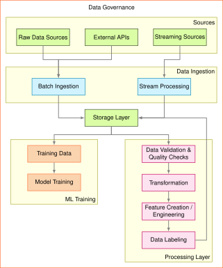](https://mlsysbook.ai/contents/core/data_engineering/4213eeaeb926472ac24f617144bb4a8344e1ec2b.svg "Figure 5: Data Pipeline Architecture: Modular pipelines ingest, process, and deliver data for machine learning tasks, enabling independent scaling of components and improved data quality control. Distinct stages (ingestion, storage, and preparation) transform raw data into a format suitable for model training and validation, forming the foundation of reliable ML systems.")
Figure 5: **Data Pipeline Architecture**: Modular pipelines ingest, process, and deliver data for machine learning tasks, enabling independent scaling of components and improved data quality control. Distinct stages (ingestion, storage, and preparation) transform raw data into a format suitable for model training and validation, forming the foundation of reliable ML systems.
As shown in the architecture diagram, ML data pipelines consist of several distinct layers: data sources, ingestion, processing, labeling, storage, and ML training ([Figure 5](https://mlsysbook.ai/contents/core/data_engineering/data_engineering.html#fig-pipeline-flow)
). Each layer plays a specific role in the data preparation workflow, and selecting appropriate technologies for each layer requires understanding how our four framework pillars manifest at each stage. Rather than treating these layers as independent components to be optimized separately, we examine how quality requirements at one stage affect scalability constraints at another, how reliability needs shape governance implementations, and how the pillars interact to determine overall system effectiveness.
Central to these design decisions, data pipeline design is constrained by storage hierarchies and I/O bandwidth limitations rather than CPU capacity. Understanding these constraints enables building efficient systems that can handle modern ML workloads. Storage hierarchy trade-offs, ranging from high-latency object storage (ideal for archival) to low-latency in-memory stores (essential for real-time serving), and bandwidth limitations (spinning disks at 100-200 MB/s versus RAM at 50-200 GB/s) shape every pipeline decision. Detailed storage architecture considerations are covered in [Section 1.9](https://mlsysbook.ai/contents/core/data_engineering/data_engineering.html#sec-data-engineering-strategic-storage-architecture-87b1)
.
Given these performance constraints, design decisions should align with specific requirements. For streaming data, consider whether you need message durability (ability to replay failed processing), ordering guarantees (maintaining event sequence), or geographic distribution. For batch processing, the key decision factors include data volume relative to memory, processing complexity, and whether computation must be distributed. Single-machine tools suffice for gigabyte-scale data, but terabyte-scale processing needs distributed frameworks that partition work across clusters. The interactions between these layers, viewed through our four-pillar lens, determine the system’s overall effectiveness and guide the specific engineering decisions we examine in the following subsections.
### Quality Through Validation and Monitoring
Quality represents the foundation of reliable ML systems, and pipelines implement quality through systematic validation and monitoring at every stage. Production experience shows that data pipeline issues represent a major source of ML failures, with studies citing 30-70% attribution rates for schema changes breaking downstream processing, distribution drift degrading model accuracy, or data corruption silently introducing errors ([Sculley et al. 2021](https://mlsysbook.ai/contents/core/data_engineering/data_engineering.html#ref-sculley2015hidden)
). These failures prove particularly insidious because they often don’t cause obvious system crashes but instead slowly degrade model performance in ways that become apparent only after affecting users. The quality pillar demands proactive monitoring and validation that catches issues before they cascade into model failures.
Understanding these metrics in practice requires examining how production teams implement monitoring at scale. Most organizations adopt severity-based alerting systems where different types of failures trigger different response protocols. The most critical alerts indicate complete system failure: the pipeline has stopped processing entirely, showing zero throughput for more than 5 minutes, or a primary data source has become completely unavailable. These situations demand immediate attention because they halt all downstream model training or serving. More subtle degradation patterns require different detection strategies. When throughput drops to 80% of baseline levels, or error rates climb above 5%, or quality metrics drift more than 2 standard deviations from training data characteristics, the system signals degradation requiring urgent but not immediate attention. These gradual failures often prove more dangerous than complete outages because they can persist undetected for hours or days, silently corrupting model inputs and degrading prediction quality.
Consider how these principles apply to a recommendation system processing user interaction events. With a baseline throughput of 50,000 records per second, the monitoring system tracks several interdependent signals. Instantaneous throughput alerts fire if processing drops below 40,000 records per second for more than 10 minutes, accounting for normal traffic variation while catching genuine capacity or processing problems. Each feature in the data stream has its own quality profile: if a feature like user\_age shows null values in more than 5% of records when the training data contained less than 1% nulls, something has likely broken in the upstream data source. Duplicate detection runs on sampled data, watching for the same event appearing multiple times—a pattern that might indicate retry logic gone wrong or a database query accidentally returning the same records repeatedly.
These monitoring dimensions become particularly important when considering end-to-end latency. The system must track not just whether data arrives, but how long it takes to flow through the entire pipeline from the moment an event occurs to when the resulting features become available for model inference. When 95th percentile[5](https://mlsysbook.ai/contents/core/data_engineering/data_engineering.html#fn5)
latency exceeds 30 seconds in a system with a 10-second service level agreement, the monitoring system needs to pinpoint which pipeline stage introduced the delay: ingestion, transformation, validation, or storage.
5 **95th percentile**: A statistical measure indicating that 95% of values fall below this threshold, commonly used in performance monitoring to capture typical worst-case behavior while excluding outliers. For latency monitoring, the 95th percentile provides more stable insights than maximum values (which may be anomalies) while revealing performance degradation that averages would hide.
6 **Kolmogorov-Smirnov test**: A non-parametric statistical test that quantifies whether two datasets come from the same distribution by measuring the maximum distance between their cumulative distribution functions. In ML systems, K-S tests detect data drift by comparing serving data against training baselines, producing p-values where values below 0.05 indicate statistically significant distribution shifts requiring investigation. When the test produces p-values below 0.05, it signals that serving and training data have diverged significantly—perhaps because user behavior has changed, or because an upstream system modification altered how features are computed.
Quality monitoring extends beyond simple schema validation to statistical properties that capture whether serving data resembles training data. Rather than just checking that values fall within valid ranges, production systems track rolling statistics over 24-hour windows. For numerical features like transaction\_amount or session\_duration, the system computes means and standard deviations continuously, then applies statistical tests like the Kolmogorov-Smirnov test[6](https://mlsysbook.ai/contents/core/data_engineering/data_engineering.html#fn6)
to compare serving distributions against training distributions.
Categorical features require different statistical approaches. Instead of comparing means and variances, monitoring systems track category frequency distributions. When new categories appear that never existed in training data, or when existing categories shift substantially in relative frequency—say, the proportion of “mobile” versus “desktop” traffic changes by more than 20%, the system flags potential data quality issues or genuine distribution shifts. This statistical vigilance catches subtle problems that simple schema validation misses entirely: imagine if age values remain in the valid range of 18-95, but the distribution shifts from primarily 25-45 year olds to primarily 65+ year olds, indicating the data source has changed in ways that will affect model performance.
Validation at the pipeline level encompasses multiple strategies working together. Schema validation executes synchronously as data enters the pipeline, rejecting malformed records immediately before they can propagate downstream. Modern tools like TensorFlow Data Validation (TFDV)[7](https://mlsysbook.ai/contents/core/data_engineering/data_engineering.html#fn7)
automatically infer schemas from training data, capturing expected data types, value ranges, and presence requirements.
7 **TensorFlow Data Validation (TFDV)**: A production-grade library for analyzing and validating ML data that automatically infers schemas, detects anomalies, and identifies training-serving skew. TFDV computes descriptive statistics, identifies data drift through distribution comparisons, and generates human-readable validation reports, integrating with TFX pipelines for automated data quality monitoring. For a feature vector containing user demographics, the inferred schema might specify that user\_age must be a 64-bit integer between 18 and 95 and cannot be null, user\_country must be a string from a specific set of country codes, and session\_duration must be a floating-point number between 0 and 7200 seconds but is optional. During serving, the validator checks each incoming record against these specifications, rejecting records with null required fields, out-of-range values, or type mismatches before they reach feature computation logic.
This synchronous validation necessarily remains simple and fast, checking properties that can be evaluated on individual records in microseconds. More sophisticated validation that requires comparing serving data against training data distributions or aggregating statistics across many records must run asynchronously to avoid blocking the ingestion pipeline. Statistical validation systems typically sample 1-10% of serving traffic—enough to detect meaningful shifts while avoiding the computational cost of analyzing every record. These samples accumulate in rolling windows, commonly 1 hour, 24 hours, and 7 days, with different windows revealing different patterns. Hourly windows detect sudden shifts like a data source failing over to a backup with different characteristics, while weekly windows reveal gradual drift in user populations or behavior.
Perhaps the most insidious validation challenge arises from training-serving skew[8](https://mlsysbook.ai/contents/core/data_engineering/data_engineering.html#fn8)
, where the same features get computed differently in training versus serving environments. This typically happens when training pipelines process data in batch using one set of libraries or logic, while serving systems compute features in real-time using different implementations. A recommendation system might compute “user\_lifetime\_purchases” in training by joining user profiles against complete transaction histories, while the serving system inadvertently uses a cached materialized view[9](https://mlsysbook.ai/contents/core/data_engineering/data_engineering.html#fn9)
updated only weekly.
8 **Training-Serving Skew**: A ML systems failure where identical features are computed differently during training versus serving, causing silent model degradation. Occurs when training uses batch processing with one implementation while serving uses real-time processing with different libraries, creating subtle differences that compound to degrade accuracy significantly without obvious errors.
9 **Materialized view**: A database optimization that pre-computes and stores query results as physical tables, trading storage space for query performance. Unlike standard views that compute results on-demand, materialized views cache expensive join and aggregation operations but require refresh strategies to maintain data freshness, creating potential training-serving skew when refresh schedules differ between environments. The resulting 15% discrepancy between training and serving features directly explains seemingly mysterious 12% accuracy drops observed in production A/B tests. Detecting training-serving skew requires infrastructure that can recompute training features on serving data for comparison. Production systems implement periodic validation where they sample raw serving data, process it through both training and serving feature pipelines, and measure discrepancies.
### Reliability Through Graceful Degradation
While quality monitoring detects issues, reliability ensures systems continue operating effectively when problems occur. Pipelines face constant challenges: data sources become temporarily unavailable, network partitions separate components, upstream schema changes break parsing logic, or unexpected load spikes exhaust resources. The reliability pillar demands systems that handle these failures gracefully rather than cascading into complete outage. This resilience comes from systematic failure analysis, intelligent error handling, and automated recovery strategies that maintain service continuity even under adverse conditions.
Systematic failure mode analysis for ML data pipelines reveals predictable patterns that require specific engineering countermeasures. Data corruption failures occur when upstream systems introduce subtle format changes, encoding issues, or field value modifications that pass basic validation but corrupt model inputs. A date field switching from “YYYY-MM-DD” to “MM/DD/YYYY” format might not trigger schema validation but will break any date-based feature computation. Schema evolution[10](https://mlsysbook.ai/contents/core/data_engineering/data_engineering.html#fn10)
failures happen when source systems add fields, rename columns, or change data types without coordination, breaking downstream processing assumptions that expected specific field names or types. Resource exhaustion manifests as gradually degrading performance when data volume growth outpaces capacity planning, eventually causing pipeline failures during peak load periods.
10 **Schema Evolution**: The challenge of managing changes to data structure over time as source systems add fields, rename columns, or modify data types. Critical for ML systems because model training expects consistent feature schemas, and schema changes can silently break feature computation or introduce training-serving skew.
11 **Dead Letter Queue**: A separate storage system for messages that fail processing after exhausting retry attempts, enabling later analysis and reprocessing without blocking the main pipeline. Essential for ML systems where data loss is unacceptable—malformed training examples can be fixed and reprocessed, while failed inference requests can be debugged to improve system robustness.
Kleppmann, Martin. 2016. _Designing Data-Intensive Applications: The Big Ideas Behind Reliable, Scalable, and Maintainable Systems_. O’Reilly Media. [http://shop.oreilly.com/product/0636920032175.do](http://shop.oreilly.com/product/0636920032175.do)
.
Building on this failure analysis, effective error handling strategies ensure problems are contained and recovered from systematically. Implementing intelligent retry logic for transient errors, such as network interruptions or temporary service outages, requires exponential backoff strategies to avoid overwhelming recovering services. A simple linear retry that attempts reconnection every second would flood a struggling service with connection attempts, potentially preventing its recovery. Exponential backoff—retrying after 1 second, then 2 seconds, then 4 seconds, doubling with each attempt—gives services breathing room to recover while still maintaining persistence. Many ML systems employ the concept of dead letter queues[11](https://mlsysbook.ai/contents/core/data_engineering/data_engineering.html#fn11)
, using separate storage for data that fails processing after multiple retry attempts. This allows for later analysis and potential reprocessing of problematic data without blocking the main pipeline ([Kleppmann 2016](https://mlsysbook.ai/contents/core/data_engineering/data_engineering.html#ref-kleppmann2017designing)
). A pipeline processing financial transactions that encounters malformed data can route it to a dead letter queue rather than losing critical records or halting all processing.
Moving beyond ad-hoc error handling, cascade failure prevention requires circuit breaker[12](https://mlsysbook.ai/contents/core/data_engineering/data_engineering.html#fn12)
patterns and bulkhead isolation to prevent single component failures from propagating throughout the system. When a feature computation service fails, the circuit breaker pattern stops calling that service after detecting repeated failures, preventing the caller from waiting on timeouts that would cascade into its own failure.
12 **Circuit Breaker**: A reliability pattern that monitors service failures and automatically stops calling a failing service after a threshold is reached, preventing cascade failures and system overload. Like an electrical circuit breaker, it has three states: closed (normal operation), open (failing service blocked), and half-open (testing if service has recovered).
Automated recovery engineering implements sophisticated strategies beyond simple retry logic. Progressive timeout increases prevent overwhelming struggling services while maintaining rapid recovery for transient issues—initial requests timeout after 1 second, but after detecting service degradation, timeouts extend to 5 seconds, then 30 seconds, giving the service time to stabilize. Multi-tier fallback systems provide degraded service when primary data sources fail: serving slightly stale cached features when real-time computation fails, or using approximate features when exact computation times out. A recommendation system unable to compute user preferences from the past 30 days might fall back to preferences from the past 90 days, providing somewhat less accurate but still useful recommendations rather than failing entirely. Comprehensive alerting and escalation procedures ensure human intervention occurs when automated recovery fails, with sufficient diagnostic information captured during the failure to enable rapid debugging.
These concepts become concrete when considering a financial ML system ingesting market data. Error handling might involve falling back to slightly delayed data sources if real-time feeds fail, while simultaneously alerting the operations team to the issue. Dead letter queues capture malformed price updates for investigation rather than dropping them silently. Circuit breakers prevent the system from overwhelming a struggling market data provider during recovery. This comprehensive approach to error management ensures that downstream processes have access to reliable, high-quality data for training and inference tasks, even in the face of the inevitable failures that occur in distributed systems at scale.
### Scalability Patterns
While quality and reliability ensure correct system operation, scalability addresses a different challenge: how systems evolve as data volumes grow and ML systems mature from prototypes to production services. Pipelines that work effectively at gigabyte scale often break at terabyte scale without architectural changes that enable distributed processing. Scalability involves designing systems that handle growing data volumes, user bases, and computational demands without requiring complete redesigns. The key insight is that scalability constraints manifest differently across pipeline stages, requiring different architectural patterns for ingestion, processing, and storage.
ML systems typically follow two primary ingestion patterns, each with distinct scalability characteristics. Batch ingestion involves collecting data in groups over a specified period before processing. This method proves appropriate when real-time data processing is not critical and data can be processed at scheduled intervals. A retail company might use batch ingestion to process daily sales data overnight, updating ML models for inventory prediction each morning. Batch processing enables efficient use of computational resources by amortizing startup costs across large data volumes—a job processing one terabyte might use 100 machines for 10 minutes, achieving better resource efficiency than maintaining always-on infrastructure.
In contrast to this scheduled approach, stream ingestion processes data in real-time as it arrives. This pattern proves crucial for applications requiring immediate data processing, scenarios where data loses value quickly, and systems that need to respond to events as they occur. A financial institution might use stream ingestion for real-time fraud detection, processing each transaction as it occurs to flag suspicious activity immediately. However, stream processing must handle backpressure[13](https://mlsysbook.ai/contents/core/data_engineering/data_engineering.html#fn13)
when downstream systems cannot keep pace—when a sudden traffic spike produces data faster than processing capacity, the system must either buffer data (requiring memory), sample (losing some data), or push back to producers (potentially causing failures). Data freshness Service Level Agreements (SLAs)[14](https://mlsysbook.ai/contents/core/data_engineering/data_engineering.html#fn14)
formalize these requirements, specifying maximum acceptable delays between data generation and availability for processing.
13 **Backpressure**: A flow control mechanism in streaming systems where downstream components signal upstream producers to slow data transmission when processing capacity is exceeded. Critical for preventing memory overflow and system crashes during traffic spikes, backpressure can be implemented through buffering, sampling, or direct producer throttling—each with different trade-offs between data loss and system stability.
14 **Service Level Agreement (SLA)**: A formal contract specifying measurable service quality metrics like latency (95th percentile response time under 100ms), availability (99.9% uptime), and throughput (process 50,000 records/second). In ML systems, SLAs often include data freshness (features available within 5 minutes of event), model accuracy (precision above 85%), and inference latency (predictions returned under 200ms).
Recognizing the limitations of either approach alone, many modern ML systems employ hybrid approaches, combining both batch and stream ingestion to handle different data velocities and use cases. This flexibility allows systems to process both historical data in batches and real-time data streams, providing a comprehensive view of the data landscape. Production systems must balance cost versus latency trade-offs: real-time processing can cost 10-100x more than batch processing. This cost differential arises from several factors: streaming systems require always-on infrastructure rather than schedulable resources, maintain redundant processing for fault tolerance, need low-latency networking and storage, and cannot benefit from the economies of scale that batch processing achieves by amortizing startup costs across large data volumes. Techniques for managing streaming systems at scale, including backpressure handling and cost optimization, are detailed in **[Chapter 13: ML Operations](https://mlsysbook.ai/contents/core/ops/ops.html#sec-ml-operations)
**.
Beyond ingestion patterns, distributed processing becomes necessary when single machines cannot handle data volumes or processing complexity. The challenge in distributed systems is that data must be partitioned across multiple computing resources, which introduces coordination overhead. Distributed coordination is limited by network round-trip times: local operations complete in microseconds while network coordination requires milliseconds, creating a 1000x latency difference. This constraint explains why operations requiring global coordination, like computing normalization statistics across 100 machines, create bottlenecks. Each partition computes local statistics quickly, but combining them requires information from all partitions, and the round-trip time for gathering results dominates total execution time.
Data locality becomes critical at this scale. Moving one terabyte of training data across the network takes 100+ seconds at 10GB/s, while local SSD access requires only 200 seconds at 5GB/s. This similar performance between network transfer and local storage drives ML system design toward compute-follows-data architectures where processing moves to data rather than data moving to processing. When processing nodes access local data at RAM speeds (50-200 GB/s) but must coordinate over networks limited to 1-10 GB/s, the bandwidth mismatch creates fundamental bottlenecks. Geographic distribution amplifies these challenges: cross-datacenter coordination must handle network latency (50-200ms between regions), partial failures during network partitions, and regulatory constraints preventing data from crossing borders. Understanding which operations parallelize easily versus those requiring expensive coordination determines system architecture and performance characteristics.
For our KWS system, these scalability patterns manifest concretely through quantitative capacity planning that dimensions infrastructure appropriately for workload requirements. Development uses batch processing on sample datasets to iterate on model architectures rapidly. Training scales to distributed processing across GPU clusters when model complexity or dataset size (23 million examples) exceeds single-machine capacity. Production deployment requires stream processing for real-time wake word detection on millions of concurrent devices. The system must handle traffic spikes when news events trigger synchronized usage—millions of users simultaneously asking about breaking news.
To make these scaling challenges concrete, consider the engineering calculations required to dimension our KWS training infrastructure. With 23 million audio samples averaging 1 second each at 16 kHz sampling rate (16-bit PCM[15](https://mlsysbook.ai/contents/core/data_engineering/data_engineering.html#fn15)
), raw storage requires approximately:
15 **Pulse Code Modulation (PCM)**: The standard digital audio representation that samples analog waveforms at regular intervals and quantizes amplitudes to discrete values. 16-bit PCM at 16 kHz captures speech adequately for recognition tasks, storing each sample as a 16-bit integer (65,536 possible values) sampled 16,000 times per second, yielding 32 KB/second of uncompressed audio data.
\\\[ \\text{Storage} = 23 \\times 10^6 \\text{ samples} \\times 1 \\text{ sec} \\times 16,000 \\text{ samples/sec} \\times 2 \\text{ bytes} = 736 \\text{ GB} \\\]
Processing these samples into MFCC features (13 coefficients, 100 frames per second) reduces storage but increases computational requirements. Feature extraction on a modern CPU processes approximately 100x real-time (100 seconds of audio per second of computation), requiring:
\\\[\\text{Processing time} = \\frac{23 \\times 10^6 \\text{ sec of audio}}{100 \\text{ speedup}} = 230,000 \\text{ sec} \\approx 64 \\text{ hours on single core}\\\]
Distributing across 64 cores reduces this to one hour, demonstrating how parallelization enables rapid iteration. Network bandwidth becomes the bottleneck when transferring training data from storage to GPU servers—at 10 GB/s network throughput, transferring 736 GB requires 74 seconds, comparable to the training epoch time itself. This analysis reveals why high-throughput storage (NVMe SSDs achieving 5-7 GB/s) and network infrastructure (25-100 Gbps interconnects) prove essential for ML workloads where data movement time rivals computation time.
Scalability architecture enables this range from development through production while maintaining efficiency at each stage, with capacity planning ensuring infrastructure appropriately dimensions for workload requirements.
### Governance Through Observability
Having addressed functional requirements through quality, reliability, and scalability, we turn to the governance pillar. The governance pillar manifests in pipelines as comprehensive observability—the ability to understand what data flows through the system, how it transforms, and who accesses it. Effective governance requires tracking data lineage from sources through transformations to final datasets, maintaining audit trails for compliance, and implementing access controls that enforce organizational policies. Unlike the other pillars that focus primarily on system functionality, governance ensures operations occur within legal, ethical, and business constraints while maintaining transparency and accountability.
Data lineage tracking captures the complete provenance of every dataset: which raw sources contributed data, what transformations were applied, when processing occurred, and what version of processing code executed. For ML systems, lineage becomes essential for debugging model behavior and ensuring reproducibility. When a model prediction proves incorrect, engineers need to trace back through the pipeline: which training data contributed to this prediction, what quality metrics did that data have, what transformations were applied, and can we recreate this exact scenario for investigation? Modern lineage systems like Apache Atlas, Amundsen, or commercial offerings instrument pipelines to automatically capture this flow. Each pipeline stage annotates data with metadata describing its provenance, creating an audit trail that enables both debugging and compliance.
Audit trails complement lineage by recording who accessed data and when. Regulatory frameworks like GDPR require organizations to demonstrate appropriate data handling, including tracking access to personal information. ML pipelines implement audit logging at data access points: when training jobs read datasets, when serving systems retrieve features, or when engineers query data for analysis. These logs typically capture user identity, timestamp, data accessed, and purpose. For a healthcare ML system, audit trails demonstrate compliance by showing that only authorized personnel accessed patient data, that access occurred for legitimate medical purposes, and that data wasn’t retained longer than allowed. The scale of audit logging in production systems can be substantial—a high-traffic recommendation system might generate millions of audit events daily—requiring efficient log storage and querying infrastructure.
Access controls enforce policies about who can read, write, or transform data at each pipeline stage. Rather than simple read/write permissions, ML systems often implement attribute-based access control where policies consider data sensitivity, user roles, and access context. A data scientist might access anonymized training data freely but require approval for raw data containing personal information. Production serving systems might read feature data but never write it, preventing accidental corruption. Access controls integrate with data catalogs that maintain metadata about data sensitivity, compliance requirements, and usage restrictions, enabling automated policy enforcement as data flows through pipelines.
Provenance metadata enables reproducibility essential for both debugging and compliance. When a model trained six months ago performed better than current models, teams need to recreate that training environment: exact data version, transformation parameters, and code versions. ML systems implement this through comprehensive metadata capture: training jobs record dataset checksums, transformation parameter values, random seeds for reproducibility, and code version hashes. Feature stores maintain historical feature values, enabling point-in-time reconstruction of training conditions. For our KWS system, this means tracking which version of forced alignment generated labels, what audio normalization parameters were applied, what synthetic data generation settings were used, and which crowdsourcing batches contributed to training data.
The integration of these governance mechanisms transforms pipelines from opaque data transformers into auditable, reproducible systems that can demonstrate appropriate data handling. This governance infrastructure proves essential not just for regulatory compliance but for maintaining trust in ML systems as they make increasingly consequential decisions affecting users’ lives.
With comprehensive pipeline architecture established—quality through validation and monitoring, reliability through graceful degradation, scalability through appropriate patterns, and governance through observability—we must now determine what actually flows through these carefully designed systems. The data sources we choose shape every downstream characteristic of our ML systems.
**Self-Check: Question 1.4**
1. Which of the following components is NOT typically part of a data pipeline architecture?
1. Model Deployment
2. Data Ingestion
3. Data Validation
4. Storage Layer
2. Explain how the four-pillar framework influences the design of data pipeline architectures in ML systems.
3. True or False: In data pipeline architecture, computational processing power is the primary constraint for system design.
4. Order the following stages of a data pipeline from initial data entry to final preparation for ML: (1) Data Validation, (2) Data Ingestion, (3) Feature Creation, (4) Storage Layer.
5. In a production system, what trade-offs would you consider when choosing between batch and stream ingestion methods?
[See Answers →](https://mlsysbook.ai/contents/core/data_engineering/data_engineering.html#quiz-answer-sec-data-engineering-data-pipeline-architecture-0005)
Strategic Data Acquisition
--------------------------
Data acquisition represents more than simply gathering training examples. It is a strategic decision that determines our system’s capabilities and limitations. The approaches we choose for sourcing training data directly shape our quality foundation, reliability characteristics, scalability potential, and governance compliance. Rather than treating data sources as independent options to be selected based on convenience or familiarity, we examine them as strategic choices that must align with our established framework requirements. Each sourcing strategy (existing datasets, web scraping, crowdsourcing, synthetic generation) offers different trade-offs across quality, cost, scale, and ethical considerations. The key insight is that no single approach satisfies all requirements; successful ML systems typically combine multiple strategies, balancing their complementary strengths against competing constraints.
Returning to our KWS system, data source decisions have profound implications across all our framework pillars, as demonstrated in our integrated case study in [Section 1.3.3](https://mlsysbook.ai/contents/core/data_engineering/data_engineering.html#sec-data-engineering-framework-application-keyword-spotting-case-study-21ff)
. Achieving 98% accuracy across diverse acoustic environments (quality pillar) requires representative data spanning accents, ages, and recording conditions. Maintaining consistent detection despite device variations (reliability pillar) demands data from varied hardware. Supporting millions of concurrent users (scalability pillar) requires data volumes that manual collection cannot economically provide. Protecting user privacy in always-listening systems (governance pillar) constrains collection methods and requires careful anonymization. These interconnected requirements demonstrate why acquisition strategy must be evaluated systematically rather than through ad-hoc source selection.
### Data Source Evaluation and Selection
Having established the strategic importance of data acquisition, we begin with quality as the primary driver. When quality requirements dominate acquisition decisions, the choice between curated datasets, expert crowdsourcing, and controlled web scraping depends on the accuracy targets, domain expertise needed, and benchmark requirements that guide model development. The quality pillar demands understanding not just that data appears correct but that it accurately represents the deployment environment and provides sufficient coverage of edge cases that might cause failures.
Platforms like [Kaggle](https://www.kaggle.com/)
and [UCI Machine Learning Repository](https://archive.ics.uci.edu/)
provide ML practitioners with ready-to-use datasets that can jumpstart system development. These pre-existing datasets are particularly valuable when building ML systems as they offer immediate access to cleaned, formatted data with established benchmarks. One of their primary advantages is cost efficiency, as creating datasets from scratch requires significant time and resources, especially when building production ML systems that need large amounts of high-quality training data. Building on this cost efficiency, many of these datasets, such as [ImageNet](https://www.image-net.org/)
, have become standard benchmarks in the machine learning community, enabling consistent performance comparisons across different models and architectures. For ML system developers, this standardization provides clear metrics for evaluating model improvements and system performance. The immediate availability of these datasets allows teams to begin experimentation and prototyping without delays in data collection and preprocessing.
Despite these advantages, ML practitioners must carefully consider the quality assurance aspects of pre-existing datasets. For instance, the ImageNet dataset was found to have label errors on 3.4% of the validation set ([Northcutt, Athalye, and Mueller 2021](https://mlsysbook.ai/contents/core/data_engineering/data_engineering.html#ref-northcutt2021pervasive)
). While popular datasets benefit from community scrutiny that helps identify and correct errors and biases, most datasets remain “untended gardens” where quality issues can significantly impact downstream system performance if not properly addressed. As ([Gebru et al. 2021](https://mlsysbook.ai/contents/core/data_engineering/data_engineering.html#ref-gebru2018datasheets)
) highlighted in her paper, simply providing a dataset without documentation can lead to misuse and misinterpretation, potentially amplifying biases present in the data.
Gebru, Timnit, Jamie Morgenstern, Briana Vecchione, Jennifer Wortman Vaughan, Hanna Wallach, Hal Daumé III, and Kate Crawford. 2021. “Datasheets for Datasets.” _Communications of the ACM_ 64 (12): 86–92. [https://doi.org/10.1145/3458723](https://doi.org/10.1145/3458723)
.
Pineau, Joelle, Philippe Vincent-Lamarre, Koustuv Sinha, Vincent Larivière, Alina Beygelzimer, Florence d’Alché-Buc, Emily Fox, and Hugo Larochelle. 2021. “Improving Reproducibility in Machine Learning Research (a Report from the Neurips 2019 Reproducibility Program).” _Journal of Machine Learning Research_ 22 (164): 1–20.
Henderson, Peter, Riashat Islam, Philip Bachman, Joelle Pineau, Doina Precup, and David Meger. 2018. “Deep Reinforcement Learning That Matters.” _Proceedings of the AAAI Conference on Artificial Intelligence_ 32 (1): 3207–14. [https://doi.org/10.1609/aaai.v32i1.11694](https://doi.org/10.1609/aaai.v32i1.11694)
.
Gudivada, Venkat N., Dhana Rao Rao, et al. 2017. “Data Quality Considerations for Big Data and Machine Learning: Going Beyond Data Cleaning and Transformations.” _IEEE Transactions on Knowledge and Data Engineering_.
Beyond quality concerns, supporting documentation accompanying existing datasets is invaluable, yet is often only present in widely-used datasets. Good documentation provides insights into the data collection process and variable definitions and sometimes even offers baseline model performances. This information not only aids understanding but also promotes reproducibility in research, a cornerstone of scientific integrity; currently, there is a crisis around improving reproducibility in machine learning systems ([Pineau et al. 2021](https://mlsysbook.ai/contents/core/data_engineering/data_engineering.html#ref-pineau2021improving)
; [Henderson et al. 2018](https://mlsysbook.ai/contents/core/data_engineering/data_engineering.html#ref-henderson2018deep)
). When other researchers have access to the same data, they can validate findings, test new hypotheses, or apply different methodologies, thus allowing us to build on each other’s work more rapidly. The challenges of data quality extend particularly to big data scenarios where volume and variety compound quality concerns ([Gudivada, Rao, et al. 2017](https://mlsysbook.ai/contents/core/data_engineering/data_engineering.html#ref-gudivada2017data)
), requiring systematic approaches to quality validation at scale.
Even with proper documentation, understanding the context in which the data was collected becomes necessary. Researchers must avoid potential overfitting when using popular datasets such as ImageNet ([Beyer et al. 2020](https://mlsysbook.ai/contents/core/data_engineering/data_engineering.html#ref-beyer2020we)
), which can lead to inflated performance metrics. Sometimes, these [datasets do not reflect the real-world data](https://venturebeat.com/uncategorized/3-big-problems-with-datasets-in-ai-and-machine-learning/)
.
Beyer, Lucas, Olivier J. Hénaff, Alexander Kolesnikov, Xiaohua Zhai, and Aäron van den Oord. 2020. “Are We Done with ImageNet?” _arXiv Preprint arXiv:2006.07159_, June. [http://arxiv.org/abs/2006.07159v1](http://arxiv.org/abs/2006.07159v1)
.
Central to these contextual concerns, a key consideration for ML systems is how well pre-existing datasets reflect real-world deployment conditions. Relying on standard datasets can create a concerning disconnect between training and production environments. This misalignment becomes particularly problematic when multiple ML systems are trained on the same datasets ([Figure 6](https://mlsysbook.ai/contents/core/data_engineering/data_engineering.html#fig-misalignment)
), potentially propagating biases and limitations throughout an entire ecosystem of deployed models.
[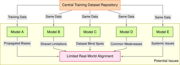](https://mlsysbook.ai/contents/core/data_engineering/468ba33927b8b88f56facc3c9e5a72db5d0773f0.svg "Figure 6: Dataset Convergence: Shared datasets can mask limitations and propagate biases across multiple machine learning systems, potentially leading to overoptimistic performance evaluations and reduced generalization to unseen data. Reliance on common datasets creates a false sense of progress within an ecosystem of models, hindering the development of robust and reliable AI applications.")
Figure 6: **Dataset Convergence**: Shared datasets can mask limitations and propagate biases across multiple machine learning systems, potentially leading to overoptimistic performance evaluations and reduced generalization to unseen data. Reliance on common datasets creates a false sense of progress within an ecosystem of models, hindering the development of robust and reliable AI applications.
For our KWS system, pre-existing datasets like Google’s Speech Commands ([Warden 2018](https://mlsysbook.ai/contents/core/data_engineering/data_engineering.html#ref-warden2018speech)
) provide essential starting points, offering carefully curated voice samples for common wake words. These datasets enable rapid prototyping and establish baseline performance metrics. However, evaluating them against our quality requirements immediately reveals coverage gaps: limited accent diversity, predominantly quiet recording environments, and support for only major languages. Quality-driven acquisition strategy recognizes these limitations and plans complementary approaches to address them, demonstrating how framework-based thinking guides source selection beyond simply choosing available datasets.
Warden, Pete. 2018. “Speech Commands: A Dataset for Limited-Vocabulary Speech Recognition.” _arXiv Preprint arXiv:1804.03209_, April. [http://arxiv.org/abs/1804.03209v1](http://arxiv.org/abs/1804.03209v1)
.
### Scalability and Cost Optimization
While quality-focused approaches excel at creating accurate, well-curated datasets, they face inherent scaling limitations. When scale requirements dominate—needing millions or billions of examples that manual curation cannot economically provide—web scraping and synthetic generation offer paths to massive datasets. The scalability pillar demands understanding the economic models underlying different acquisition strategies: cost per labeled example, throughput limitations, and how these scale with data volume. What proves cost-effective at thousand-example scale often becomes prohibitive at million-example scale, while approaches that require high setup costs amortize favorably across large volumes.
Web scraping offers a powerful approach to gathering training data at scale, particularly in domains where pre-existing datasets are insufficient. This automated technique for extracting data from websites has become essential for modern ML system development, enabling teams to build custom datasets tailored to their specific needs. When human-labeled data is scarce, web scraping demonstrates its value. Consider computer vision systems: major datasets like [ImageNet](https://www.image-net.org/)
and [OpenImages](https://storage.googleapis.com/openimages/web/index.html)
were built through systematic web scraping, significantly advancing the field of computer vision.
Expanding beyond these computer vision applications, the impact of web scraping extends well beyond image recognition systems. In natural language processing, web-scraped data has enabled the development of increasingly sophisticated ML systems. Large language models, such as ChatGPT and Claude, rely on vast amounts of text scraped from the public internet and media to learn language patterns and generate responses ([Groeneveld et al. 2024](https://mlsysbook.ai/contents/core/data_engineering/data_engineering.html#ref-groeneveld2024olmo)
). Similarly, specialized ML systems like GitHub’s Copilot demonstrate how targeted web scraping, in this case of code repositories, can create powerful domain-specific assistants ([Chen et al. 2021](https://mlsysbook.ai/contents/core/data_engineering/data_engineering.html#ref-chen2021evaluating)
).
Groeneveld, Dirk, Iz Beltagy, Pete Walsh, Akshita Bhagia, Rodney Kinney, Oyvind Tafjord, Ananya Harsh Jha, et al. 2024. “OLMo: Accelerating the Science of Language Models.” _arXiv Preprint arXiv:2402.00838_, February. [http://arxiv.org/abs/2402.00838v4](http://arxiv.org/abs/2402.00838v4)
.
Chen, Mark, Jerry Tworek, Heewoo Jun, Qiming Yuan, Henrique Ponde de Oliveira Pinto, Jared Kaplan, Harri Edwards, et al. 2021. “Evaluating Large Language Models Trained on Code.” _arXiv Preprint arXiv:2107.03374_, July. [http://arxiv.org/abs/2107.03374v2](http://arxiv.org/abs/2107.03374v2)
.
Building on these foundational developments, production ML systems often require continuous data collection to maintain relevance and performance. Web scraping facilitates this by gathering structured data like stock prices, weather patterns, or product information for analytical applications. This continuous collection introduces unique challenges for ML systems. Data consistency becomes crucial, as variations in website structure or content formatting can disrupt the data pipeline and affect model performance. Proper data management through databases or warehouses becomes essential not just for storage, but for maintaining data quality and enabling model updates.
However, alongside these powerful capabilities, web scraping presents several challenges that ML system developers must carefully consider. Legal and ethical constraints can limit data collection, as not all websites permit scraping, and violating these restrictions can have [serious consequences](https://hls.harvard.edu/today/does-chatgpt-violate-new-york-times-copyrights/)
. When building ML systems with scraped data, teams must carefully document data sources and ensure compliance with terms of service and copyright laws. Privacy considerations become important when dealing with user-generated content, often requiring systematic anonymization procedures.
Complementing these legal and ethical constraints, technical limitations also affect the reliability of web-scraped training data. Rate limiting by websites can slow data collection, while the dynamic nature of web content can introduce inconsistencies that impact model training. As shown in [Figure 7](https://mlsysbook.ai/contents/core/data_engineering/data_engineering.html#fig-traffic-light)
, web scraping can yield unexpected or irrelevant data, for example, historical images appearing in contemporary image searches, that can pollute training datasets and degrade model performance. These issues highlight the importance of thorough data validation and cleaning processes in ML pipelines built on web-scraped data.
[](https://mlsysbook.ai/contents/core/data_engineering/images/jpg/1914_traffic.jpeg "Figure 7: Data Source Noise: Web scraping introduces irrelevant or outdated data into training sets, requiring systematic data validation and cleaning to maintain model performance and prevent spurious correlations. Historical images appearing in contemporary searches exemplify this noise, underscoring the need for careful filtering and quality control in web-sourced datasets. Source: Vox.")
Figure 7: **Data Source Noise**: Web scraping introduces irrelevant or outdated data into training sets, requiring systematic data validation and cleaning to maintain model performance and prevent spurious correlations. Historical images appearing in contemporary searches exemplify this noise, underscoring the need for careful filtering and quality control in web-sourced datasets. Source: Vox.
Crowdsourcing offers another scalable approach, leveraging distributed human computation to accelerate dataset creation. Platforms like [Amazon Mechanical Turk](https://www.mturk.com/)
exemplify how crowdsourcing facilitates this process by distributing annotation tasks to a global workforce. This enables rapid collection of labels for complex tasks such as sentiment analysis, image recognition, and speech transcription, significantly expediting the data preparation phase. One of the most impactful examples of crowdsourcing in machine learning is the creation of the [ImageNet dataset](https://image-net.org/)
. ImageNet, which revolutionized computer vision, was built by distributing image labeling tasks to contributors via Amazon Mechanical Turk. The contributors categorized millions of images into thousands of classes, enabling researchers to train and benchmark models for a wide variety of visual recognition tasks.
Building on this massive labeling effort, the dataset’s availability spurred advancements in deep learning, including the breakthrough AlexNet model in 2012 ([Krizhevsky, Sutskever, and Hinton 2017](https://mlsysbook.ai/contents/core/data_engineering/data_engineering.html#ref-krizhevsky2012imagenet)
) that demonstrated the power of large-scale neural networks and showed how large-scale, crowdsourced datasets could drive innovation. ImageNet’s success highlights how leveraging a diverse group of contributors for annotation can enable machine learning systems to achieve unprecedented performance. Extending beyond academic research, another example of crowdsourcing’s potential is Google’s [Crowdsource](https://crowdsource.google.com/)
, a platform where volunteers contribute labeled data to improve AI systems in applications like language translation, handwriting recognition, and image understanding.
Beyond these static dataset creation efforts, crowdsourcing has also been instrumental in applications beyond traditional dataset annotation. For instance, the navigation app [Waze](https://www.waze.com/)
uses crowdsourced data from its users to provide real-time traffic updates, route suggestions, and incident reporting. These diverse applications highlight one of the primary advantages of crowdsourcing: its scalability. By distributing microtasks to a large audience, projects can process enormous volumes of data quickly and cost-effectively. This scalability is particularly beneficial for machine learning systems that require extensive datasets to achieve high performance. The diversity of contributors introduces a wide range of perspectives, cultural insights, and linguistic variations, enriching datasets and improving models’ ability to generalize across populations.
Complementing this scalability advantage, flexibility is a key benefit of crowdsourcing. Tasks can be adjusted dynamically based on initial results, allowing for iterative improvements in data collection. For example, Google’s [reCAPTCHA](https://www.google.com/recaptcha/about/)
system uses crowdsourcing to verify human users while simultaneously labeling datasets for training machine learning models.
Moving beyond human-generated data entirely, synthetic data generation represents the ultimate scalability solution, creating unlimited training examples through algorithmic generation rather than manual collection. This approach changes the economics of data acquisition by removing human labor from the equation. As [Figure 8](https://mlsysbook.ai/contents/core/data_engineering/data_engineering.html#fig-synthetic-data)
illustrates, synthetic data combines with historical datasets to create larger, more diverse training sets that would be impractical to collect manually.
[](https://mlsysbook.ai/contents/core/data_engineering/9bbc195613b2889c8434fe22b8cc694ba65e2f91.svg "Figure 8: Synthetic Data Augmentation: Combining algorithmically generated data with historical datasets expands training set size and diversity, mitigating limitations caused by scarce or biased real-world data and improving model generalization. This approach enables robust machine learning system development when acquiring sufficient real-world data is impractical or unethical. Source: anylogic.")
Figure 8: **Synthetic Data Augmentation**: Combining algorithmically generated data with historical datasets expands training set size and diversity, mitigating limitations caused by scarce or biased real-world data and improving model generalization. This approach enables robust machine learning system development when acquiring sufficient real-world data is impractical or unethical. Source: [anylogic](https://www.anylogic.com/features/artificial-intelligence/synthetic-data/)
.
Building on this foundation, advancements in generative modeling techniques have greatly enhanced the quality of synthetic data. Modern AI systems can produce data that closely resembles real-world distributions, making it suitable for applications ranging from computer vision to natural language processing. For example, generative models have been used to create synthetic images for object recognition tasks, producing diverse datasets that closely match real-world images. Similarly, synthetic data has been leveraged to simulate speech patterns, enhancing the robustness of voice recognition systems.
Beyond these quality improvements, synthetic data has become particularly valuable in domains where obtaining real-world data is either impractical or costly. The automotive industry has embraced synthetic data to train autonomous vehicle systems; there are only so many cars you can physically crash to get crash-test data that might help an ML system know how to avoid crashes in the first place. Capturing real-world scenarios, especially rare edge cases such as near-accidents or unusual road conditions, is inherently difficult. Synthetic data allows researchers to [simulate these scenarios in a controlled virtual environment](https://www.nvidia.com/en-us/use-cases/autonomous-vehicle-simulation/)
, ensuring that models are trained to handle a wide range of conditions. This approach has proven invaluable for advancing the capabilities of self-driving cars.
Complementing these safety-critical applications, another important application of synthetic data lies in augmenting existing datasets. Introducing variations into datasets enhances model robustness by exposing the model to diverse conditions. For instance, in speech recognition, data augmentation techniques like SpecAugment ([Park et al. 2019](https://mlsysbook.ai/contents/core/data_engineering/data_engineering.html#ref-park2019specaugment)
) introduce noise, shifts, or pitch variations, enabling models to generalize better across different environments and speaker styles. This principle extends to other domains as well, where synthetic data can fill gaps in underrepresented scenarios or edge cases.
Park, Daniel S., William Chan, Yu Zhang, Chung-Cheng Chiu, Barret Zoph, Ekin D. Cubuk, and Quoc V. Le. 2019. “SpecAugment: A Simple Data Augmentation Method for Automatic Speech Recognition.” _arXiv Preprint arXiv:1904.08779_, April. [http://arxiv.org/abs/1904.08779v3](http://arxiv.org/abs/1904.08779v3)
.
Werchniak, Andrew, Roberto Barra Chicote, Yuriy Mishchenko, Jasha Droppo, Jeff Condal, Peng Liu, and Anish Shah. 2021. “Exploring the Application of Synthetic Audio in Training Keyword Spotters.” In _ICASSP 2021 - 2021 IEEE International Conference on Acoustics, Speech and Signal Processing (ICASSP)_, 7993–96. IEEE; IEEE. [https://doi.org/10.1109/icassp39728.2021.9413448](https://doi.org/10.1109/icassp39728.2021.9413448)
.
For our KWS system, the scalability pillar drove the need for 23 million training examples across 50 languages—a volume that manual collection cannot economically provide. Web scraping supplements baseline datasets with diverse voice samples from video platforms. Crowdsourcing enables targeted collection for underrepresented languages. Synthetic data generation fills remaining gaps through speech synthesis ([Werchniak et al. 2021](https://mlsysbook.ai/contents/core/data_engineering/data_engineering.html#ref-werchniak2021exploring)
) and audio augmentation, creating unlimited wake word variations across acoustic environments, speaker characteristics, and background conditions. This comprehensive multi-source strategy demonstrates how scalability requirements shape acquisition decisions, with each approach contributing specific capabilities to the overall data ecosystem.
### Reliability Across Diverse Conditions
Beyond quality and scale considerations, the reliability pillar addresses a critical question: will our collected data enable models that perform consistently across the deployment environment’s full range of conditions? A dataset might achieve high quality by established metrics yet fail to support reliable production systems if it doesn’t capture the diversity encountered during deployment. Coverage requirements for robust models extend beyond simple volume to encompass geographic diversity, demographic representation, temporal variation, and edge case inclusion that stress-test model behavior.
Understanding coverage requirements requires examining potential failure modes. Geographic bias occurs when training data comes predominantly from specific regions, causing models to underperform in other areas. A study of image datasets found significant geographic skew, with image recognition systems trained on predominantly Western imagery performing poorly on images from other regions ([Wang et al. 2019](https://mlsysbook.ai/contents/core/data_engineering/data_engineering.html#ref-wang2019balanced)
). Demographic bias emerges when training data doesn’t represent the full user population, potentially causing discriminatory outcomes. Temporal variation matters when phenomena change over time—a fraud detection model trained only on historical data may fail against new fraud patterns. Edge case collection proves particularly challenging yet critical, as rare scenarios often represent high-stakes situations where failures cause the most harm.
The challenge of edge case collection becomes apparent in autonomous vehicle development. While normal driving conditions are easy to capture through test fleet operation, near-accidents, unusual pedestrian behavior, or rare weather conditions occur infrequently. Synthetic data generation helps address this by simulating rare scenarios, but validating that synthetic examples accurately represent real edge cases requires careful engineering. Some organizations employ targeted data collection where test drivers deliberately create edge cases or where engineers identify scenarios from incident reports that need better coverage.
Dataset convergence, illustrated in [Figure 6](https://mlsysbook.ai/contents/core/data_engineering/data_engineering.html#fig-misalignment)
earlier, represents another reliability challenge. When multiple systems train on identical datasets, they inherit identical blind spots and biases. An entire ecosystem of models may fail on the same edge cases because all trained on data with the same coverage gaps. This systemic risk motivates diverse data sourcing strategies where each organization collects supplementary data beyond common benchmarks, ensuring their models develop different strengths and weaknesses rather than shared failure modes.
For our KWS system, reliability manifests as consistent wake word detection across acoustic environments from quiet bedrooms to noisy streets, across accents from various geographic regions, and across age ranges from children to elderly speakers. The data sourcing strategy explicitly addresses these diversity requirements: web scraping captures natural speech variation from diverse video sources, crowdsourcing targets underrepresented demographics and environments, and synthetic data systematically explores the parameter space of acoustic conditions. Without this deliberate diversity in sourcing, the system might achieve high accuracy on test sets while failing unreliably in production deployment.
### Governance and Ethics in Sourcing
The governance pillar in data acquisition encompasses legal compliance, ethical treatment of data contributors, privacy protection, and transparency about data origins and limitations. Unlike the other pillars that focus on system capabilities, governance ensures data sourcing occurs within appropriate legal and ethical boundaries. The consequences of governance failures extend beyond system performance to reputational damage, legal liability, and potential harm to individuals whose data was improperly collected or used.
Legal constraints significantly limit data collection methods across different jurisdictions and domains. Not all websites permit scraping, and violating these restrictions can have serious consequences, as ongoing litigation around training data for large language models demonstrates. Copyright law governs what publicly available content can be used for training, with different standards emerging across jurisdictions. Terms of service agreements may prohibit using data for ML training even when technically accessible. Privacy regulations like GDPR in Europe and CCPA in California impose strict requirements on personal data collection, requiring consent, enabling deletion requests, and sometimes demanding explanations of algorithmic decisions ([Wachter, Mittelstadt, and Russell 2017](https://mlsysbook.ai/contents/core/data_engineering/data_engineering.html#ref-wachter2017counterfactual)
). Healthcare data falls under additional regulations like HIPAA in the United States, requiring specific safeguards for patient information. Organizations must carefully navigate these legal frameworks, documenting data sources and ensuring compliance throughout the acquisition process.
Wachter, Sandra, Brent Mittelstadt, and Chris Russell. 2017. “Counterfactual Explanations Without Opening the Black Box: Automated Decisions and the GDPR.” _SSRN Electronic Journal_ 31: 841. [https://doi.org/10.2139/ssrn.3063289](https://doi.org/10.2139/ssrn.3063289)
.
Beyond legal compliance, ethical sourcing requires fair treatment of human contributors. The crowdsourcing example we examined earlier—where [OpenAI outsourced data annotation to workers in Kenya](https://time.com/6247678/openai-chatgpt-kenya-workers/)
paying as little as $1.32 per hour for reviewing traumatic content—highlights governance failures that can occur when economic pressures override ethical considerations. Many workers reportedly suffered psychological harm from exposure to disturbing material without adequate mental health support. This case underscores power imbalances that can emerge when outsourcing data work to economically disadvantaged regions. The lack of fair compensation, inadequate support for workers dealing with traumatic content, and insufficient transparency about working conditions represent governance failures that affect human welfare beyond just system performance.
Industry-wide standards for ethical crowdsourcing have begun emerging in response to such concerns. Fair compensation means paying at least local minimum wages, ideally benchmarked against comparable work in workers’ regions. Worker wellbeing requires providing mental health resources for those dealing with sensitive content, limiting exposure to traumatic material, and ensuring reasonable working conditions. Transparency demands clear communication about task purposes, how contributions will be used, and worker rights. Organizations like the Partnership on AI have published guidelines for ethical crowdwork, establishing baselines for acceptable practices.
While quality, scalability, and reliability focus on system capabilities, the governance pillar ensures our data acquisition occurs within appropriate ethical and legal boundaries. Privacy protection forms another critical governance concern, particularly when sourcing data involving individuals who didn’t explicitly consent to ML training use. Anonymization emerges as a critical capability when handling sensitive data. From a systems engineering perspective, anonymization represents more than regulatory compliance; it constitutes a core design constraint affecting data pipeline architecture, storage strategies, and processing efficiency. ML systems must handle sensitive data throughout their lifecycle: during collection, storage, transformation, model training, and even in error logs and debugging outputs. A single privacy breach can compromise not just individual records but entire datasets, making the system unusable for future development.
Practitioners have developed a range of anonymization techniques to mitigate privacy risks. The most straightforward approach, masking, involves altering or obfuscating sensitive values so that they cannot be directly traced back to the original data subject. For instance, digits in financial account numbers or credit card numbers can be replaced with asterisks, fixed dummy characters, or hashed values to protect sensitive information during display or logging.
Building on this direct protection approach, generalization reduces the precision or granularity of data to decrease the likelihood of re-identification. Instead of revealing an exact date of birth or address, the data is aggregated into broader categories such as age ranges or zip code prefixes. For example, a user’s exact age of 37 might be generalized to an age range of 30-39, while their exact address might be bucketed to city-level granularity. This technique reduces re-identification risk by sharing data in aggregated form, though careful granularity selection is crucial—too coarse loses analytical value while too fine may still enable re-identification under certain conditions.
While generalization reduces data precision, pseudonymization takes a different approach by replacing direct identifiers—names, Social Security numbers, email addresses—with artificial identifiers or “pseudonyms.” These pseudonyms must not reveal or be easily traceable to the original data subject, enabling analysis that links records for the same individual without exposing their identity.
Moving beyond simple identifier replacement, k-anonymity provides a more formal approach, ensuring that each record in a dataset is indistinguishable from at least k-1 other records. This is achieved by suppressing or generalizing quasi-identifiers—attributes that in combination could be used to re-identify individuals, such as zip code, age, and gender. For example, if k=5, every record must share the same combination of quasi-identifiers with at least four other records, preventing attackers from pinpointing individuals simply by looking at these attributes. This approach provides formal privacy guarantees but may require significant data distortion and doesn’t protect against homogeneity or background knowledge attacks.
At the most sophisticated end of this spectrum, differential privacy ([Dwork, n.d.](https://mlsysbook.ai/contents/core/data_engineering/data_engineering.html#ref-dwork2008differential)
) adds carefully calibrated noise or randomized data perturbations to query results or datasets. The goal is to ensure that including or excluding any single individual’s data doesn’t significantly affect outputs, thereby concealing their presence. Introduced noise is controlled by the ε parameter in ε-Differential Privacy, balancing data utility and privacy guarantees. This approach provides strong mathematical privacy guarantees and sees wide use in academic and industrial settings, though added noise can affect data accuracy and model performance, requiring careful parameter tuning to balance privacy and usefulness.
Dwork, Cynthia. n.d. “Differential Privacy: A Survey of Results.” In _Theory and Applications of Models of Computation_, 1–19. Springer Berlin Heidelberg. [https://doi.org/10.1007/978-3-540-79228-4\\\_1](https://doi.org/10.1007/978-3-540-79228-4/_1)
.
[Table 2](https://mlsysbook.ai/contents/core/data_engineering/data_engineering.html#tbl-anonymization-comparison)
summarizes the key characteristics of each anonymization approach to help practitioners select appropriate techniques based on their specific privacy requirements and data utility needs.
Table 2: Anonymization Techniques Comparison
| | | | | |
| --- | --- | --- | --- | --- |
| **Masking** | High | Low-Medium | Simple | Displaying sensitive data |
| **Generalization** | Medium | Medium | Moderate | Age ranges, location bucketing |
| **Pseudonymization** | High | Medium | Moderate | Individual tracking needed |
| **K-anonymity** | Low-Medium | High | Complex | Formal privacy guarantees |
| **Differential Privacy** | Medium | Very High | Complex | Statistical guarantees |
As the comparison table illustrates, effective data anonymization balances privacy and utility. Techniques such as masking, generalization, pseudonymization, k-anonymity, and differential privacy each target different aspects of re-identification risk. By carefully selecting and combining these methods, organizations can responsibly derive value from sensitive datasets while respecting the privacy rights and expectations of the individuals represented within them.
For our KWS system, governance constraints shape acquisition throughout. Voice data inherently contains biometric information requiring privacy protection, driving decisions about anonymization, consent requirements, and data retention policies. Multilingual support raises equity concerns—will the system work only for commercially valuable languages or also serve smaller linguistic communities? Fair crowdsourcing practices ensure that annotators providing voice samples or labeling receive appropriate compensation and understand how their contributions will be used. Transparency about data sources and limitations enables users to understand system capabilities and potential biases. These governance considerations don’t just constrain acquisition but shape which approaches are ethically acceptable and legally permissible.
### Integrated Acquisition Strategy
Having examined how each pillar shapes acquisition choices, we now see why real-world ML systems rarely use a single acquisition method in isolation. Instead, they combine approaches strategically to balance competing pillar requirements, recognizing that each method contributes complementary strengths. The art of data acquisition lies in understanding how these sources work together to create datasets that satisfy quality, scalability, reliability, and governance constraints simultaneously.
Our KWS system exemplifies this integrated approach. Google’s Speech Commands dataset provides a quality-assured baseline enabling rapid prototyping and establishing performance benchmarks. However, evaluating this against our requirements reveals gaps: limited accent diversity, coverage of only major languages, predominantly clean recording environments. Web scraping addresses some gaps by gathering diverse voice samples from video platforms and speech databases, capturing natural speech patterns across varied acoustic conditions. This scales beyond what manual collection could provide while maintaining reasonable quality through automated filtering.
Crowdsourcing fills targeted gaps that neither existing datasets nor web scraping adequately address: underrepresented accents, specific demographic groups, or particular acoustic environments identified as weak points. By carefully designing crowdsourcing tasks with clear guidelines and quality control, the system balances scale with quality while ensuring ethical treatment of contributors. Synthetic data generation completes the picture by systematically exploring the parameter space: varying background noise levels, speaker ages, microphone characteristics, and wake word pronunciations. This addresses the long tail of rare conditions that are impractical to collect naturally while enabling controlled experiments about which acoustic variations most affect model performance.
The synthesis of these approaches demonstrates how our framework guides strategy. Quality requirements drive use of curated datasets and expert review. Scalability needs motivate synthetic generation and web scraping. Reliability demands mandate diverse sourcing across demographics and environments. Governance constraints shape consent requirements, anonymization practices, and fair compensation policies. Rather than selecting sources based on convenience, the integrated strategy systematically addresses each pillar’s requirements through complementary methods.
The diversity achieved through multi-source acquisition—crowdsourced audio with varying quality, synthetic data with perfect consistency, web-scraped content with unpredictable formats—creates specific challenges at the boundary where external data enters our controlled pipeline environment.
**Self-Check: Question 1.5**
1. Which of the following is a primary consideration when selecting a data acquisition strategy for an ML system?
1. The availability of pre-existing datasets
2. Alignment with framework requirements
3. The convenience of the data source
4. The familiarity of the data source
2. Explain the trade-offs between using web scraping and crowdsourcing for data acquisition in terms of scalability and ethical considerations.
3. True or False: Relying solely on pre-existing datasets can lead to a disconnect between training and production environments.
4. What is a potential drawback of using synthetic data generation as a data acquisition strategy?
1. Potential lack of real-world relevance
2. Limited control over data quality
3. High cost of data labeling
4. Inability to scale data collection
5. In a production system, how might you apply an integrated data acquisition strategy to ensure both scalability and reliability?
[See Answers →](https://mlsysbook.ai/contents/core/data_engineering/data_engineering.html#quiz-answer-sec-data-engineering-strategic-data-acquisition-9ff8)
Data Ingestion
--------------
Data ingestion represents the critical junction where carefully acquired data enters our ML systems, transforming from diverse external formats into standardized pipeline inputs. This boundary layer must handle the heterogeneity resulting from our multi-source acquisition strategy while maintaining the quality, reliability, scalability, and governance standards we’ve established. This transformation from external sources into controlled pipeline environments presents several challenges that manifest distinctly across our framework pillars. The quality pillar demands validation that catches issues at the entry point before they propagate downstream. The reliability pillar requires error handling that maintains operation despite source failures and data anomalies. The scalability pillar necessitates throughput optimization that handles growing data volumes and velocity. The governance pillar enforces access controls and audit trails at the system boundary where external data enters trusted environments. Ingestion represents a critical boundary where careful engineering prevents problems from entering the pipeline while enabling the data flow that ML systems require.
### Batch vs. Streaming Ingestion Patterns
To address these ingestion challenges systematically, ML systems typically follow two primary patterns that reflect different approaches to data flow timing and processing. Each pattern has distinct characteristics and use cases that shape how systems balance latency, throughput, cost, and complexity. Understanding when to apply batch versus streaming ingestion—or combinations thereof—requires analyzing workload characteristics against our framework requirements.
Batch ingestion involves collecting data in groups or batches over a specified period before processing. This method proves appropriate when real-time data processing is not critical and data can be processed at scheduled intervals. The batch approach enables efficient use of computational resources by amortizing startup costs across large data volumes and processing when resources are available or least expensive. For example, a retail company might use batch ingestion to process daily sales data overnight, updating their ML models for inventory prediction each morning ([Akidau et al. 2015](https://mlsysbook.ai/contents/core/data_engineering/data_engineering.html#ref-akidau2015dataflow)
). The batch job might process gigabytes of transaction data using dozens of machines for 30 minutes, then release those resources for other workloads. This scheduled processing proves far more cost-effective than maintaining always-on infrastructure, particularly when slight staleness in predictions doesn’t affect business outcomes.
Akidau, Tyler, Robert Bradshaw, Craig Chambers, Slava Chernyak, Rafael J. Fernández-Moctezuma, Reuven Lax, Sam McVeety, et al. 2015. “The Dataflow Model: A Practical Approach to Balancing Correctness, Latency, and Cost in Massive-Scale, Unbounded, Out-of-Order Data Processing.” _Proceedings of the VLDB Endowment_ 8 (12): 1792–1803. [https://doi.org/10.14778/2824032.2824076](https://doi.org/10.14778/2824032.2824076)
.
Batch processing also simplifies error handling and recovery. When a batch job fails midway, the system can retry the entire batch or resume from checkpoints without complex state management. Data scientists can easily inspect failed batches, understand what went wrong, and reprocess after fixes. The deterministic nature of batch processing—processing the same input data always produces the same output—simplifies debugging and validation. These characteristics make batch ingestion attractive for ML workflows even when real-time processing is technically feasible but not required.
In contrast to this scheduled approach, stream ingestion processes data in real-time as it arrives, consuming events continuously rather than waiting to accumulate batches. This pattern proves crucial for applications requiring immediate data processing, scenarios where data loses value quickly, and systems that need to respond to events as they occur. A financial institution might use stream ingestion for real-time fraud detection, processing each transaction as it occurs to flag suspicious activity immediately before completing the transaction. The value of fraud detection drops dramatically if detection occurs hours after the fraudulent transaction completes—by then money has been transferred and accounts compromised.
However, stream processing introduces complexity that batch processing avoids. The system must handle backpressure when downstream systems cannot keep pace with incoming data rates. During traffic spikes, when a sudden surge produces data faster than processing capacity, the system must either buffer data (requiring memory and introducing latency), sample (losing some data), or push back to producers (potentially causing their failures). Data freshness Service Level Agreements (SLAs) formalize these requirements, specifying maximum acceptable delays between data generation and availability for processing. Meeting a 100-millisecond freshness SLA requires different infrastructure than meeting a 1-hour SLA, affecting everything from networking to storage to processing architectures.
Recognizing the limitations of either approach alone, many modern ML systems employ hybrid approaches, combining both batch and stream ingestion to handle different data velocities and use cases. This flexibility allows systems to process both historical data in batches and real-time data streams, providing a comprehensive view of the data landscape. A recommendation system might use streaming ingestion for real-time user interactions—clicks, views, purchases—to update session-based recommendations immediately, while using batch ingestion for overnight processing of user profiles, item features, and collaborative filtering models that don’t require real-time updates.
Production systems must balance cost versus latency trade-offs when selecting patterns: real-time processing can cost 10-100x more than batch processing. This cost differential arises from several factors: streaming systems require always-on infrastructure rather than schedulable resources that can spin up and down based on workload; maintain redundant processing for fault tolerance to ensure no events are lost; need low-latency networking and storage to meet millisecond-scale SLAs; and cannot benefit from economies of scale that batch processing achieves by amortizing startup costs across large data volumes. A batch job processing one terabyte might use 100 machines for 10 minutes, while a streaming system processing the same data over 24 hours needs dedicated resources continuously available. This 100x difference in cost per byte processed drives many architectural decisions about which data truly requires real-time processing versus what can tolerate batch delays.
### ETL and ELT Comparison
Beyond choosing ingestion patterns based on timing requirements, designing effective data ingestion pipelines requires understanding the differences between Extract, Transform, Load (ETL)[16](https://mlsysbook.ai/contents/core/data_engineering/data_engineering.html#fn16)
and Extract, Load, Transform (ELT)[17](https://mlsysbook.ai/contents/core/data_engineering/data_engineering.html#fn17)
approaches, as illustrated in [Figure 9](https://mlsysbook.ai/contents/core/data_engineering/data_engineering.html#fig-etl-vs-elt)
. These paradigms determine when data transformations occur relative to the loading phase, significantly impacting the flexibility and efficiency of ML pipelines. The choice between ETL and ELT affects where computational resources are consumed, how quickly data becomes available for analysis, and how easily transformation logic can evolve as requirements change.
16 **Extract, Transform, Load (ETL)**: A data processing pattern where raw data is extracted from sources, transformed (cleaned, aggregated, validated) in a separate processing layer, then loaded into storage. For example, a traditional ETL pipeline might extract customer purchase logs, transform them by removing duplicates and aggregating daily totals in Apache Spark, then load only the aggregated results into a data warehouse. Ensures only high-quality data reaches storage but requires reprocessing all data when transformation logic changes.
17 **Extract, Load, Transform (ELT)**: A data processing pattern where raw data is extracted and immediately loaded into scalable storage, then transformed using the storage system’s computational resources. For example, an ELT pipeline might extract raw clickstream events directly into a data lake like S3, then use SQL queries in a system like Snowflake or BigQuery to create multiple transformed views: user sessions for analytics, feature vectors for ML models, and aggregated metrics for dashboards. Enables faster iteration and multiple transformation variants but requires more storage capacity and careful governance of raw data.
[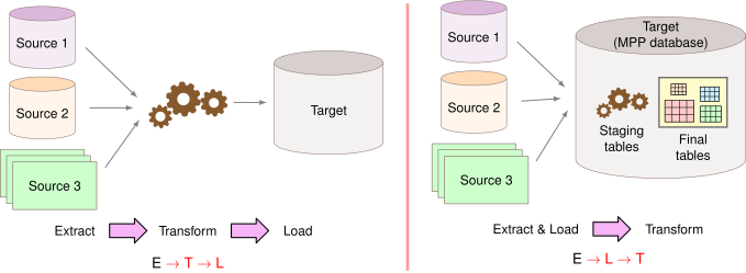](https://mlsysbook.ai/contents/core/data_engineering/ecff59fc5f0797ded4b8d4637d9036cc3e85ac9f.svg "Figure 9: Data Pipeline Architectures: ETL pipelines transform data before loading it into a data warehouse, while ELT pipelines load raw data first and transform it within the warehouse, impacting system flexibility and resource allocation for machine learning workflows. Choosing between ETL and ELT depends on data volume, transformation complexity, and the capabilities of the target data storage system.")
Figure 9: **Data Pipeline Architectures**: ETL pipelines transform data _before_ loading it into a data warehouse, while ELT pipelines load raw data first and transform it within the warehouse, impacting system flexibility and resource allocation for machine learning workflows. Choosing between ETL and ELT depends on data volume, transformation complexity, and the capabilities of the target data storage system.
ETL is a well-established paradigm in which data is first gathered from a source, then transformed to match the target schema or model, and finally loaded into a data warehouse or other repository. This approach typically results in data being stored in a ready-to-query format, which can be advantageous for ML systems that require consistent, pre-processed data. The transformation step occurs in a separate processing layer before data reaches the warehouse, enabling validation and standardization before persistence. For instance, an ML system predicting customer churn might use ETL to standardize and aggregate customer interaction data from multiple sources—converting different timestamp formats to UTC, normalizing text encodings to UTF-8, and computing aggregate features like “total purchases last 30 days”—before loading into a format suitable for model training ([Inmon 2005](https://mlsysbook.ai/contents/core/data_engineering/data_engineering.html#ref-inmon2005building)
).
Inmon, W. H. 2005. _Building the Data Warehouse_. John Wiley Sons.
The advantages of ETL become apparent in scenarios with well-defined schemas and transformation requirements. Only cleaned, validated, transformed data reaches the warehouse, reducing storage requirements and simplifying downstream queries. Security and privacy compliance can be enforced during transformation, ensuring sensitive data is masked or encrypted before reaching storage. Quality validation occurs before loading, preventing corrupted or invalid data from entering the warehouse. For ML systems with stable feature pipelines and clear data quality requirements, ETL provides a clean separation between messy source data and curated training data.
However, ETL can be less flexible when schemas or requirements change frequently, a common occurrence in evolving ML projects. When transformation logic changes—adding new features, modifying aggregations, or correcting bugs—all source data must be reprocessed through the ETL pipeline to update the warehouse. This reprocessing can take hours or days for large datasets, slowing iteration velocity during ML development. The transformation layer requires dedicated infrastructure and expertise, adding operational complexity and cost to the data pipeline.
This is where the ELT approach offers advantages. ELT reverses the order by first loading raw data and then applying transformations as needed within the target system. This method is often seen in modern data lake or schema-on-read environments, allowing for a more agile approach when addressing evolving analytical needs in ML systems. Raw source data is loaded quickly into scalable storage, with transformations applied using the warehouse’s computational resources. Modern cloud data warehouses like BigQuery, Snowflake, and Redshift provide massive computational capacity that can execute complex transformations on terabyte-scale data in minutes.
By deferring transformations, ELT can accommodate varying uses of the same dataset, which is particularly useful in exploratory data analysis phases of ML projects or when multiple models with different data requirements are being developed simultaneously. One team might compute daily aggregates while another computes hourly aggregates, each transforming the same raw data differently. When transformation logic bugs are discovered, teams can reprocess data by simply rerunning transformation queries rather than re-ingesting from sources. This flexibility accelerates ML experimentation where feature engineering requirements evolve rapidly.
However, ELT places greater demands on storage systems and query engines, which must handle large amounts of unprocessed information. Raw data storage grows larger than transformed data, increasing costs. Query performance may suffer when transformations execute repeatedly on the same raw data rather than reading pre-computed results. Privacy and compliance become more complex when raw sensitive data persists in storage rather than being masked during ingestion.
In practice, many ML systems employ hybrid approaches, selecting ETL or ELT on a case-by-case basis depending on the specific requirements of each data source or ML model. For example, a system might use ETL for structured data from relational databases where schemas are well-defined and stable, while employing ELT for unstructured data like text or images where transformation requirements may evolve as the ML models are refined. High-volume clickstream data might use ELT to enable rapid loading and flexible transformation, while sensitive financial data might use ETL to enforce encryption and masking before persistence.
When implementing streaming components within ETL/ELT architectures, distributed systems principles become critical. The CAP theorem[18](https://mlsysbook.ai/contents/core/data_engineering/data_engineering.html#fn18)
fundamentally constrains streaming system design choices. Apache Kafka[19](https://mlsysbook.ai/contents/core/data_engineering/data_engineering.html#fn19)
prioritizes consistency and partition tolerance, making it ideal for reliable event ordering but potentially experiencing availability issues during network partitions. Apache Pulsar emphasizes availability and partition tolerance, providing better fault tolerance but with relaxed consistency guarantees. Amazon Kinesis balances all three properties through careful configuration but requires understanding these trade-offs for proper deployment.
18 **CAP Theorem**: A fundamental distributed systems principle stating that any distributed data system can guarantee at most two of three properties: Consistency (all nodes see the same data simultaneously), Availability (system remains operational), and Partition tolerance (system continues despite network failures). Critical for ML systems where different workloads prioritize different properties.
19 **Apache Kafka**: A distributed streaming platform designed for high-throughput, low-latency data streaming with strong durability guarantees. Provides ordered, replicated logs that enable reliable event processing at scale, making it essential for ML systems requiring real-time data ingestion, feature serving, and model prediction logging.
### Multi-Source Integration Strategies
Regardless of whether ETL or ELT approaches are used, integrating diverse data sources represents a key challenge in data ingestion for ML systems. Data may originate from various sources including databases, APIs, file systems, and IoT devices. Each source may have its own data format, access protocol, and update frequency. The integration challenge lies not just in connecting to these sources but in normalizing their disparate characteristics into a unified pipeline that subsequent processing stages can consume reliably.
Given this source diversity, ML engineers must develop robust connectors or adapters for each data source to effectively integrate these sources. These connectors handle the specifics of data extraction, including authentication, rate limiting, and error handling. For example, when integrating with a REST API, the connector would manage API keys, respect rate limits specified in API documentation or HTTP headers, and handle HTTP status codes appropriately—retrying on transient errors (500, 503), aborting on authentication failures (401, 403), and backing off when rate limited (429). A well-designed connector abstracts these details from downstream processing, presenting a consistent interface regardless of whether data originates from APIs, databases, or file systems.
Beyond basic connectivity, source integration often involves data transformation at the ingestion point. This might include parsing JSON[20](https://mlsysbook.ai/contents/core/data_engineering/data_engineering.html#fn20)
or XML responses into structured formats, converting timestamps to a standard timezone and format (typically UTC and ISO 8601), or performing basic data cleaning operations like trimming whitespace or normalizing text encodings. The goal is to standardize the data format as it enters the ML pipeline, simplifying downstream processing. These transformations differ from the business logic transformations in ETL or ELT—they address technical format variations rather than semantic transformation of content.
20 **JavaScript Object Notation (JSON)**: A lightweight, text-based data interchange format using human-readable key-value pairs and arrays. Ubiquitous in web APIs and modern data systems due to its simplicity and language-agnostic parsing, though less storage-efficient than binary formats like Parquet for large-scale ML datasets.
In addition to data format standardization, it’s essential to consider the reliability and availability of data sources. Some sources may experience downtime or have inconsistent data quality. Implementing retry mechanisms with exponential backoff handles transient failures gracefully. Data quality checks at ingestion catch systematic problems early—if a source suddenly starts producing null values for previously required fields, immediate detection prevents corrupted data from flowing downstream. Fallback procedures enable continued operation when primary sources fail: switching to backup data sources, serving cached data, or degrading gracefully rather than failing completely. A stock price ingestion system might fall back to delayed prices if real-time feeds fail, maintaining service with slightly stale data rather than complete outage.
### Case Study: Selecting Ingestion Patterns for KWS
Applying these ingestion concepts to our KWS system, production implementations demonstrate both streaming and batch patterns working in concert, reflecting the dual operational modes we established during problem definition. The ingestion architecture directly implements requirements from our four-pillar framework: quality through validation of audio characteristics, reliability through consistent operation despite source diversity, scalability through handling millions of concurrent streams, and governance through source authentication and tracking.
The streaming ingestion pattern handles real-time audio data from active devices where wake words must be detected within our 200 millisecond latency requirement. This requires careful implementation of publish-subscribe mechanisms using systems like Apache Kafka that buffer incoming audio data and enable parallel processing across multiple inference servers. The streaming path prioritizes our reliability and scalability pillars: maintaining consistent low-latency operation despite varying device loads and network conditions while handling millions of concurrent audio streams from deployed devices.
Parallel to this real-time processing, batch ingestion handles data for model training and updates. This includes the diverse data sources we established during acquisition: new wake word recordings from crowdsourcing efforts discussed in [Section 1.5](https://mlsysbook.ai/contents/core/data_engineering/data_engineering.html#sec-data-engineering-strategic-data-acquisition-9ff8)
, synthetic data from voice generation systems that address coverage gaps we identified, and validated user interactions that provide real-world examples of both successful detections and false rejections. The batch processing typically follows an ETL pattern where audio data undergoes preprocessing—normalization to standard volume levels, filtering to remove extreme noise, and segmentation into consistent durations—before being stored in formats optimized for model training. This processing addresses our quality pillar by ensuring training data undergoes consistent transformations that preserve the acoustic characteristics distinguishing wake words from background speech.
Integrating these diverse data sources presents unique challenges for KWS systems. Real-time audio streams require rate limiting to prevent system overload during usage spikes—imagine millions of users simultaneously asking their voice assistants about breaking news. Crowdsourced data needs systematic validation to ensure recording quality meets the specifications we established during problem definition: adequate signal-to-noise ratios, appropriate speaker distances, and correct labeling. Synthetic data must be verified for realistic representation of wake word variations rather than generating acoustically implausible samples that would mislead model training.
The sophisticated error handling mechanisms required by voice interaction systems become apparent when processing real-time audio. Dead letter queues store failed recognition attempts for subsequent analysis, helping identify patterns in false negatives or system failures that might indicate acoustic conditions we didn’t adequately cover during data collection. For example, a smart home device processing the wake word “Alexa” must validate several audio quality metrics: signal-to-noise ratio above our minimum threshold established during requirements definition, appropriate sample rate matching training data specifications, recording duration within expected bounds of one to two seconds, and speaker proximity indicators suggesting the utterance was directed at the device rather than incidental speech. Invalid samples route to dead letter queues for analysis rather than discarding them entirely—these failures often reveal edge cases requiring attention in the next model iteration. Valid samples flow through to real-time processing for wake word detection while simultaneously being logged for potential inclusion in future training data, demonstrating how production systems continuously improve through careful data engineering.
This ingestion architecture completes the boundary layer where external data enters our controlled pipeline. With reliable ingestion established—validating data quality, handling errors gracefully, scaling to required throughput, and maintaining governance controls—we now turn to systematic data processing that transforms ingested raw data into ML-ready features while maintaining the training-serving consistency essential for production systems.
**Self-Check: Question 1.6**
1. Which of the following is a key advantage of batch ingestion in ML systems?
1. Real-time processing of data as it arrives
2. Immediate detection of data anomalies as they occur
3. Efficient use of computational resources by processing data at scheduled intervals
4. Handling data spikes by buffering or sampling data
2. Explain the trade-offs between using ETL and ELT approaches in ML data pipelines.
3. Order the following steps in a typical ETL pipeline: (1) Load data into storage, (2) Extract data from sources, (3) Transform data to match target schema.
4. What is a primary challenge of stream ingestion in ML systems?
1. High computational cost due to always-on infrastructure
2. Complex error handling and recovery
3. Inability to handle large data volumes
4. High latency in data processing
[See Answers →](https://mlsysbook.ai/contents/core/data_engineering/data_engineering.html#quiz-answer-sec-data-engineering-data-ingestion-5dfc)
Systematic Data Processing
--------------------------
With reliable data ingestion established, we enter the most technically challenging phase of the pipeline: systematic data processing. Here, a fundamental requirement—applying identical transformations during training and serving—becomes the source of approximately 70% of production ML failures ([Sculley et al. 2021](https://mlsysbook.ai/contents/core/data_engineering/data_engineering.html#ref-sculley2015hidden)
). This striking statistic underscores why training-serving consistency must serve as the central organizing principle for all processing decisions.
Sculley, David, Gary Holt, Daniel Golovin, Eugene Davydov, Todd Phillips, Dietmar Ebner, Vinay Chaudhary, Michael Young, Jean-Francois Crespo, and Dan Dennison. 2021. “Technical Debt in Machine Learning Systems.” In _Technical Debt in Practice_, 177–92. The MIT Press. [https://doi.org/10.7551/mitpress/12440.003.0011](https://doi.org/10.7551/mitpress/12440.003.0011)
.
Data processing implements the quality requirements defined in our problem definition phase, transforming raw data into ML-ready formats while maintaining reliability and scalability standards. Processing decisions must preserve data integrity while improving model readiness, all while adhering to governance principles throughout the transformation pipeline. Every transformation—from normalization parameters to categorical encodings to feature engineering logic—must be applied identically in both contexts. Consider a simple example: normalizing transaction amounts during training by removing currency symbols and converting to floats, but forgetting to apply identical preprocessing during serving. This seemingly minor inconsistency can degrade model accuracy by 20-40%, as the model receives differently formatted inputs than it was trained on. The severity of this problem makes training-serving consistency the central organizing principle for processing system design.
For our KWS system, processing decisions directly impact all four pillars as established in our problem definition ([Section 1.3.3](https://mlsysbook.ai/contents/core/data_engineering/data_engineering.html#sec-data-engineering-framework-application-keyword-spotting-case-study-21ff)
). Quality transformations must preserve acoustic characteristics essential for wake word detection while standardizing across diverse recording conditions. Reliability requires consistent processing despite varying audio formats collected through our multi-source acquisition strategy. Scalability demands efficient algorithms that handle millions of audio streams from deployed devices. Governance ensures privacy-preserving transformations that protect user voice data throughout processing.
### Ensuring Training-Serving Consistency
We begin with quality as the cornerstone of data processing. Here, the quality pillar manifests as ensuring that transformations applied during training match exactly those applied during serving. This consistency challenge extends beyond just applying the same code—it requires that parameters computed on training data (normalization constants, encoding dictionaries, vocabulary mappings) are stored and reused during serving. Without this discipline, models receive fundamentally different inputs during serving than they were trained on, causing performance degradation that’s often subtle and difficult to debug.
Data cleaning involves identifying and correcting errors, inconsistencies, and inaccuracies in datasets. Raw data frequently contains issues such as missing values, duplicates, or outliers that can significantly impact model performance if left unaddressed. The key insight is that cleaning operations must be deterministic and reproducible: given the same input, cleaning must produce the same output whether executed during training or serving. This requirement shapes which cleaning techniques are safe to use in production ML systems.
Data cleaning might involve removing duplicate records based on deterministic keys, handling missing values through imputation or deletion using rules that can be applied consistently, and correcting formatting inconsistencies systematically. For instance, in a customer database, names might be inconsistently capitalized or formatted. A data cleaning process would standardize these entries, ensuring that “John Doe,” “john doe,” and “DOE, John” are all treated as the same entity. The cleaning rules—convert to title case, reorder to “First Last” format—must be captured in code that executes identically in training and serving. As emphasized throughout this chapter, every cleaning operation must be applied identically in both contexts to maintain system reliability.
Outlier detection and treatment is another important aspect of data cleaning, but one that introduces consistency challenges. Outliers can sometimes represent valuable information about rare events, but they can also result from measurement errors or data corruption. ML practitioners must carefully consider the nature of their data and the requirements of their models when deciding how to handle outliers. Simple threshold-based outlier removal (removing values more than 3 standard deviations from the mean) maintains training-serving consistency if the mean and standard deviation are computed on training data and reused during serving. However, more sophisticated outlier detection methods that consider relationships between features or temporal patterns require careful engineering to ensure consistent application.
Quality assessment goes hand in hand with data cleaning, providing a systematic approach to evaluating the reliability and usefulness of data. This process involves examining various aspects of data quality, including accuracy, completeness, consistency, and timeliness. In production systems, data quality degrades in subtle ways that basic metrics miss: fields that never contain nulls suddenly show sparse patterns, numeric distributions drift from their training ranges, or categorical values appear that weren’t present during model development.
To address these subtle degradation patterns, production quality monitoring requires specific metrics beyond simple missing value counts as discussed in [Section 1.4.1](https://mlsysbook.ai/contents/core/data_engineering/data_engineering.html#sec-data-engineering-quality-validation-monitoring-5f2a)
. Critical indicators include null value patterns by feature (sudden increases suggest upstream failures), count anomalies (10x increases often indicate data duplication or pipeline errors), value range violations (prices becoming negative, ages exceeding realistic bounds), and join failure rates between data sources. Statistical drift detection[21](https://mlsysbook.ai/contents/core/data_engineering/data_engineering.html#fn21)
becomes essential by monitoring means, variances, and quantiles of features over time to catch gradual degradation before it impacts model performance. For example, in an e-commerce recommendation system, the average user session length might gradually increase from 8 minutes to 12 minutes over six months due to improved site design, but a sudden drop to 3 minutes suggests a data collection bug.
21 **Data Drift**: The phenomenon where statistical properties of production data change over time, diverging from training data distributions and silently degrading model performance. Can occur gradually (user behavior evolving) or suddenly (system changes), requiring continuous monitoring of feature distributions, means, variances, and categorical frequencies to detect before accuracy drops.
Supporting these monitoring requirements, quality assessment tools range from simple statistical measures to complex machine learning-based approaches. Data profiling tools provide summary statistics and visualizations that help identify potential quality issues, while advanced techniques employ unsupervised learning algorithms to detect anomalies or inconsistencies in large datasets. Establishing clear quality metrics and thresholds ensures that data entering the ML pipeline meets necessary standards for reliable model training and inference. The key is maintaining the same quality standards and validation logic across training and serving to prevent quality issues from creating training-serving skew.
Transformation techniques convert data from its raw form into a format more suitable for analysis and modeling. This process can include a wide range of operations, from simple conversions to complex mathematical transformations. Central to effective transformation, common transformation tasks include normalization and standardization, which scale numerical features to a common range or distribution. For example, in a housing price prediction model, features like square footage and number of rooms might be on vastly different scales. Normalizing these features ensures that they contribute more equally to the model’s predictions ([Bishop 2006](https://mlsysbook.ai/contents/core/data_engineering/data_engineering.html#ref-bishop2006pattern)
). Maintaining training-serving consistency requires that normalization parameters (mean, standard deviation) computed on training data be stored and applied identically during serving. This means persisting these parameters alongside the model itself—often in the model artifact or a separate parameter file—and loading them during serving initialization.
Bishop, Christopher M. 2006. _Pattern Recognition and Machine Learning_. Springer.
Beyond numerical scaling, other transformations might involve encoding categorical variables, handling date and time data, or creating derived features. For instance, one-hot encoding is often used to convert categorical variables into a format that can be readily understood by many machine learning algorithms. Categorical encodings must handle both the categories present during training and unknown categories encountered during serving. A robust approach computes the category vocabulary during training (the set of all observed categories), persists it with the model, and during serving either maps unknown categories to a special “unknown” token or uses default values. Without this discipline, serving encounters categories the model never saw during training, potentially causing errors or degraded performance.
Feature engineering is the process of using domain knowledge to create new features that make machine learning algorithms work more effectively. This step is often considered more of an art than a science, requiring creativity and deep understanding of both the data and the problem at hand. Feature engineering might involve combining existing features, extracting information from complex data types, or creating entirely new features based on domain insights. For example, in a retail recommendation system, engineers might create features that capture the recency, frequency, and monetary value of customer purchases, known as RFM analysis ([Kuhn and Johnson 2013](https://mlsysbook.ai/contents/core/data_engineering/data_engineering.html#ref-kuhn2013applied)
).
Kuhn, Max, and Kjell Johnson. 2013. _Applied Predictive Modeling_. Springer New York. [https://doi.org/10.1007/978-1-4614-6849-3](https://doi.org/10.1007/978-1-4614-6849-3)
.
Given these creative possibilities, the importance of feature engineering cannot be overstated. Well-engineered features can often lead to significant improvements in model performance, sometimes outweighing the impact of algorithm selection or hyperparameter tuning. However, the creativity required for feature engineering must be balanced against the consistency requirements of production systems. Every engineered feature must be computed identically during training and serving. This means that feature engineering logic should be implemented in libraries or modules that can be shared between training and serving code, rather than being reimplemented separately. Many organizations build feature stores, discussed in [Section 1.9.4](https://mlsysbook.ai/contents/core/data_engineering/data_engineering.html#sec-data-engineering-feature-stores-bridging-training-serving-fce5)
, specifically to ensure feature computation consistency across environments.
Applying these processing concepts to our KWS system, the audio recordings flowing through our ingestion pipeline—whether from crowdsourcing, synthetic generation, or real-world captures—require careful cleaning to ensure reliable wake word detection. Raw audio data often contains imperfections that our problem definition anticipated: background noise from various environments (quiet bedrooms to noisy industrial settings), clipped signals from recording level issues, varying volumes across different microphones and speakers, and inconsistent sampling rates from diverse capture devices. The cleaning pipeline must standardize these variations while preserving the acoustic characteristics that distinguish wake words from background speech—a quality-preservation requirement that directly impacts our 98% accuracy target.
Quality assessment for KWS extends the general principles with audio-specific metrics. Beyond checking for null values or schema conformance, our system tracks background noise levels (signal-to-noise ratio above 20 decibels), audio clarity scores (frequency spectrum analysis), and speaking rate consistency (wake word duration within 500-800 milliseconds). The quality assessment pipeline automatically flags recordings where background noise would prevent accurate detection, where wake words are spoken too quickly or unclearly for the model to distinguish them, or where clipping or distortion has corrupted the audio signal. This automated filtering ensures only high-quality samples reach model development, preventing the “garbage in, garbage out” cascade we identified in [Figure 3](https://mlsysbook.ai/contents/core/data_engineering/data_engineering.html#fig-cascades)
.
Transforming audio data for KWS involves converting raw waveforms into formats suitable for ML models while maintaining training-serving consistency. As shown in [Figure 10](https://mlsysbook.ai/contents/core/data_engineering/data_engineering.html#fig-spectrogram-example)
, the transformation pipeline converts audio signals into standardized feature representations—typically Mel-frequency cepstral coefficients (MFCCs)[22](https://mlsysbook.ai/contents/core/data_engineering/data_engineering.html#fn22)
or spectrograms[23](https://mlsysbook.ai/contents/core/data_engineering/data_engineering.html#fn23)
—that emphasize speech-relevant characteristics while reducing noise and variability across different recording conditions.
22 **Mel-frequency cepstral coefficients (MFCCs)**: A compact representation of audio that captures spectral envelope characteristics crucial for speech recognition. MFCCs model human auditory perception by applying mel-scale filtering (emphasizing frequencies humans hear best) followed by discrete cosine transformation, typically extracting 13-39 coefficients that encode timbral properties while discarding pitch information irrelevant for phoneme identification.
23 **Spectrogram**: A visual representation of audio showing frequency content over time, computed via Short-Time Fourier Transform (STFT) that applies FFT to overlapping windows. In ML systems, spectrograms serve as 2D image-like inputs where the x-axis represents time, y-axis represents frequency, and intensity shows amplitude, enabling convolutional neural networks to process audio as visual patterns. This transformation must be identical in training and serving: if training computes features with one FFT window size but serving uses another, the model receives fundamentally different inputs that degrade our accuracy target. Feature engineering focuses on extracting characteristics that help distinguish wake words from background speech: energy distribution across frequency bands, pitch contours that capture prosody, and duration patterns that differentiate deliberate wake word pronunciations from accidental similar sounds.
[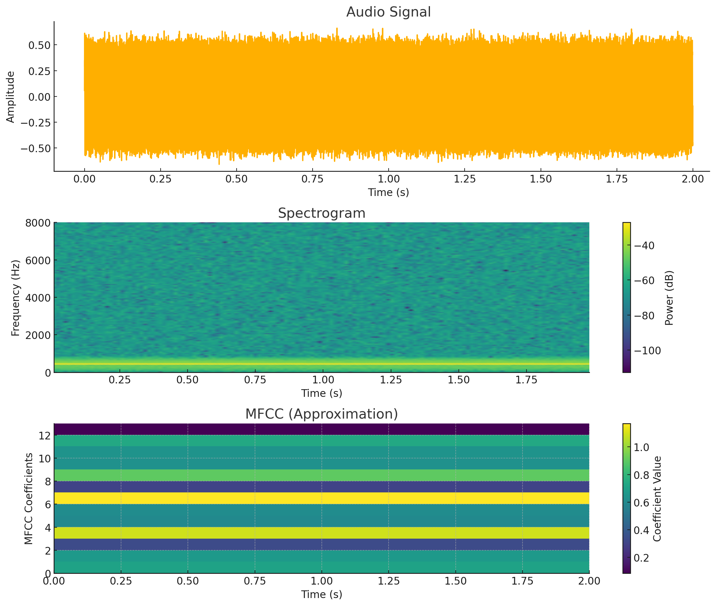](https://mlsysbook.ai/contents/core/data_engineering/images/png/kws_spectrogram.png "Figure 10: Audio Feature Transformation: Advanced audio features compress raw audio waveforms into representations that emphasize perceptually relevant characteristics for machine learning tasks. This transformation reduces noise and data dimensionality while preserving essential speech information, improving model performance in applications like keyword spotting.")
Figure 10: **Audio Feature Transformation**: Advanced audio features compress raw audio waveforms into representations that emphasize perceptually relevant characteristics for machine learning tasks. This transformation reduces noise and data dimensionality while preserving essential speech information, improving model performance in applications like keyword spotting.
### Building Idempotent Data Transformations
Building on quality foundations, we turn to reliability. While quality focuses on what transformations produce, reliability ensures how consistently they operate. Processing reliability means transformations produce identical outputs given identical inputs, regardless of when, where, or how many times they execute. This property, called idempotency, proves essential for production ML systems where processing may be retried due to failures, where data may be reprocessed to fix bugs, or where the same data flows through multiple processing paths.
To understand idempotency intuitively, consider a light switch. Flipping the switch to the “on” position turns the light on. Flipping it to “on” again leaves the light on; the operation can be repeated without changing the outcome. This is idempotent behavior. In contrast, a toggle switch that changes state with each press is not idempotent: pressing it repeatedly alternates between on and off states. In data processing, we want light switch behavior where reapplying the same transformation yields the same result, not toggle switch behavior where repeated application changes the outcome unpredictably.
Idempotent transformations enable reliable error recovery. When a processing job fails midway, the system can safely retry processing the same data without worrying about duplicate transformations or inconsistent state. A non-idempotent transformation might append data to existing records, so retrying would create duplicates. An idempotent transformation would upsert data (insert if not exists, update if exists), so retrying produces the same final state. This distinction becomes critical in distributed systems where partial failures are common and retries are the primary recovery mechanism.
Handling partial processing failures requires careful state management. Processing pipelines should be designed so that each stage can be retried independently without affecting other stages. Checkpoint-restart mechanisms enable recovery from the last successful processing state rather than restarting from scratch. For long-running data processing jobs operating on terabyte-scale datasets, checkpointing progress every few minutes means a failure near the end requires reprocessing only recent data rather than the entire dataset. The checkpoint logic must carefully track what data has been processed and what remains, ensuring no data is lost or processed twice.
Deterministic transformations are those that always produce the same output for the same input, without dependence on external factors like time, random numbers, or mutable global state. Transformations that depend on current time (e.g., computing “days since event” based on current date) break determinism—reprocessing historical data would produce different results. The solution is to capture temporal reference points explicitly: instead of “days since event,” compute “days from event to reference date” where reference date is fixed and persisted. Random operations should use seeded random number generators where the seed is derived deterministically from input data, ensuring reproducibility.
For our KWS system, reliability requires reproducible feature extraction. Audio preprocessing must be deterministic: given the same raw audio file, the same MFCC features are always computed regardless of when processing occurs or which server executes it. This enables debugging model behavior (can always recreate exact features for a problematic example), reprocessing data when bugs are fixed (produces consistent results), and distributed processing (different workers produce identical features from the same input). The processing code captures all parameters—FFT window size, hop length, number of MFCC coefficients—in configuration that’s versioned alongside the code, ensuring reproducibility across time and execution environments.
### Scaling Through Distributed Processing
With quality and reliability established, we face the challenge of scale. As datasets grow larger and ML systems become more complex, the scalability of data processing becomes the limiting factor. Consider the data processing stages we’ve discussed—cleaning, quality assessment, transformation, and feature engineering. When these operations must handle terabytes of data, a single machine becomes insufficient. The cleaning techniques that work on gigabytes of data in memory must be redesigned to work across distributed systems.
These challenges manifest when quality assessment must process data faster than it arrives, when feature engineering operations require computing statistics across entire datasets before transforming individual records, and when transformation pipelines create bottlenecks at massive volumes. Processing must scale from development (gigabytes on laptops) through production (terabytes across clusters) while maintaining consistent behavior.
To address these scaling bottlenecks, data must be partitioned across multiple computing resources, which introduces coordination challenges. Distributed coordination is fundamentally limited by network round-trip times: local operations complete in microseconds while network coordination requires milliseconds, creating a 1000x latency difference. This constraint explains why operations requiring global coordination (like computing normalization statistics across 100 machines) create bottlenecks. Each partition computes local statistics quickly, but combining them requires information from all partitions.
Data locality becomes critical at this scale. Moving one terabyte of training data across the network takes 100+ seconds at 10 gigabytes per second, while local SSD access requires only 200 seconds at 5 gigabytes per second, driving ML system design toward compute-follows-data architectures. When processing nodes access local data at RAM speeds (50-200 gigabytes per second) but must coordinate over networks limited to 1-10 gigabytes per second, the bandwidth mismatch creates fundamental bottlenecks. Geographic distribution amplifies these challenges: cross-datacenter coordination must handle network latency (50-200 milliseconds between regions), partial failures, and regulatory constraints preventing data from crossing borders. Understanding which operations parallelize easily versus those requiring expensive coordination determines system architecture and performance characteristics.
Single-machine processing suffices for surprisingly large workloads when engineered carefully. Modern servers with 256 gigabytes RAM can process datasets of several terabytes using out-of-core processing that streams data from disk. Libraries like Dask or Vaex enable pandas-like APIs that automatically stream and parallelize computations across multiple cores. Before investing in distributed processing infrastructure, teams should exhaust single-machine optimization: using efficient data formats (Parquet[24](https://mlsysbook.ai/contents/core/data_engineering/data_engineering.html#fn24)
instead of CSV), minimizing memory allocations, leveraging vectorized operations, and exploiting multi-core parallelism. The operational simplicity of single-machine processing—no network coordination, no partial failures, simple debugging—makes it preferable when performance is adequate.
24 **Parquet**: A columnar storage format optimized for analytical workloads, storing data by column rather than row to enable reading only required features and achieve superior compression. Critical for ML systems where training typically accesses subsets of columns from large datasets, delivering 5-10x I/O reduction compared to row-based formats like CSV.
Distributed processing frameworks become necessary when data volumes or computational requirements exceed single-machine capacity, but the speedup achievable through parallelization faces fundamental limits described by Amdahl’s Law:
\\\[\\text{Speedup} \\leq \\frac{1}{S + \\frac{P}{N}}\\\]
where \\(S\\) represents the serial fraction of work that cannot parallelize, \\(P\\) the parallel fraction, and \\(N\\) the number of processors. This explains why distributing our KWS feature extraction across 64 cores achieves only a 64x speedup when the work is embarrassingly parallel (\\(S \\approx 0\\)), but coordination-heavy operations like computing global normalization statistics might achieve only 10x speedup even with 64 cores due to the serial aggregation phase. Understanding this relationship guides architectural decisions: operations with high serial fractions should run on fewer, faster cores rather than many slower cores, while highly parallel workloads benefit from maximum distribution as examined further in **[Chapter 8: AI Training](https://mlsysbook.ai/contents/core/training/training.html#sec-ai-training)
**.
Apache Spark provides a distributed computing framework that parallelizes transformations across clusters of machines, handling data partitioning, task scheduling, and fault tolerance automatically. Beam provides a unified API for both batch and streaming processing, enabling the same transformation logic to run on multiple execution engines (Spark, Flink, Dataflow). TensorFlow’s tf.data API optimizes data loading pipelines for ML training, supporting distributed reading, prefetching, and transformation. The choice of framework depends on whether processing is batch or streaming, how transformations parallelize, and what execution environment is available.
Another important consideration is the balance between preprocessing and on-the-fly computation. While extensive preprocessing can speed up model training and inference, it can also lead to increased storage requirements and potential data staleness. Production systems often implement hybrid approaches, preprocessing computationally expensive features while computing rapidly changing features on-the-fly. This balance depends on storage costs, computation resources, and freshness requirements specific to each use case. Features that are expensive to compute but change slowly (user demographic summaries, item popularity scores) benefit from preprocessing. Features that change rapidly (current session state, real-time inventory levels) must be computed on-the-fly despite computational cost.
For our KWS system, scalability manifests at multiple stages. Development uses single-machine processing on sample datasets to iterate rapidly. Training at scale requires distributed processing when dataset size (23 million examples) exceeds single-machine capacity or when multiple experiments run concurrently. The processing pipeline parallelizes naturally: audio files are independent, so transforming them requires no coordination between workers. Each worker reads its assigned audio files from distributed storage, computes features, and writes results back—a trivially parallel pattern achieving near-linear scalability. Production deployment requires real-time processing on edge devices with severe resource constraints (our 16 kilobyte memory limit), necessitating careful optimization and quantization to fit processing within device capabilities.
### Tracking Data Transformation Lineage
Completing our four-pillar view of data processing, governance ensures accountability and reproducibility. The governance pillar requires tracking what transformations were applied, when they executed, which version of processing code ran, and what parameters were used. This transformation lineage enables reproducibility essential for debugging, compliance with regulations requiring explainability, and iterative improvement when transformation bugs are discovered. Without comprehensive lineage, teams cannot reproduce training data, cannot explain why models make specific predictions, and cannot safely fix processing bugs without risking inconsistency.
Transformation versioning captures which version of processing code produced each dataset. When transformation logic changes—fixing a bug, adding features, or improving quality—the version number increments. Datasets are tagged with the transformation version that created them, enabling identification of all data requiring reprocessing when bugs are fixed. This versioning extends beyond just code versions to capture the entire processing environment: library versions (different NumPy versions may produce slightly different numerical results), runtime configurations (environment variables affecting behavior), and execution infrastructure (CPU architecture affecting floating-point precision).
Parameter tracking maintains the specific values used during transformation. For normalization, this means storing the mean and standard deviation computed on training data. For categorical encoding, this means storing the vocabulary (set of all observed categories). For feature engineering, this means storing any constants, thresholds, or parameters used in feature computation. These parameters are typically serialized alongside model artifacts, ensuring serving uses identical parameters to training. Modern ML frameworks like TensorFlow and PyTorch provide mechanisms for bundling preprocessing parameters with models, simplifying deployment and ensuring consistency.
Processing lineage for reproducibility tracks the complete transformation history from raw data to final features. This includes which raw data files were read, what transformations were applied in what order, what parameters were used, and when processing occurred. Lineage systems like Apache Atlas, Amundsen, or commercial offerings instrument pipelines to automatically capture this flow. When model predictions prove incorrect, engineers can trace back through lineage: which training data contributed to this behavior, what quality scores did that data have, what transformations were applied, and can we recreate this exact scenario to investigate?
Code version ties processing results to the exact code that produced them. When processing code lives in version control (Git), each dataset should record the commit hash of the code that created it. This enables recreating the exact processing environment: checking out the specific code version, installing dependencies listed at that version, and running processing with identical parameters. Container technologies like Docker simplify this by capturing the entire processing environment (code, dependencies, system libraries) in an immutable image that can be rerun months or years later with identical results.
For our KWS system, transformation governance tracks audio processing parameters that critically affect model behavior. When audio is normalized to standard volume, the reference volume level is persisted. When FFT transforms audio to frequency domain, the window size, hop length, and window function (Hamming, Hanning, etc.) are recorded. When MFCCs are computed, the number of coefficients, frequency range, and mel filterbank parameters are captured. This comprehensive parameter tracking enables several critical capabilities: reproducing training data exactly when debugging model failures, validating that serving uses identical preprocessing to training, and systematically studying how preprocessing choices affect model accuracy. Without this governance infrastructure, teams resort to manual documentation that inevitably becomes outdated or incorrect, leading to subtle training-serving skew that degrades production performance.
### End-to-End Processing Pipeline Design
Integrating these cleaning, assessment, transformation, and feature engineering steps, processing pipelines bring together the various data processing steps into a coherent, reproducible workflow. These pipelines ensure that data is consistently prepared across training and inference stages, reducing the risk of data leakage and improving the reliability of ML systems. Pipeline design determines how easily teams can iterate on processing logic, how well processing scales as data grows, and how reliably systems maintain training-serving consistency.
Modern ML frameworks and tools often provide capabilities for building and managing data processing pipelines. For instance, Apache Beam and TensorFlow Transform allow developers to define data processing steps that can be applied consistently during both model training and serving. The choice of data processing framework must align with the broader ML framework ecosystem discussed in **[Chapter 7: AI Frameworks](https://mlsysbook.ai/contents/core/frameworks/frameworks.html#sec-ai-frameworks)
**, where framework-specific data loaders and preprocessing utilities can significantly impact development velocity and system performance.
Beyond tool selection, effective pipeline design involves considerations such as modularity, scalability, and version control. Modular pipelines allow for easy updates and maintenance of individual processing steps. Each transformation stage should be implemented as an independent module with clear inputs and outputs, enabling testing in isolation and replacement without affecting other stages. Version control for pipelines is crucial, ensuring that changes in data processing can be tracked and correlated with changes in model performance. When model accuracy drops, version control enables identifying whether processing changes contributed to the degradation.
This modular breakdown of pipeline components is well illustrated by TensorFlow Extended in [Figure 11](https://mlsysbook.ai/contents/core/data_engineering/data_engineering.html#fig-tfx-pipeline-example)
, which shows the complete flow from initial data ingestion through to final model deployment. The figure demonstrates how data flows through validation, transformation, and feature engineering stages before reaching model training. Each component in the pipeline can be versioned, tested, and scaled independently while maintaining overall system consistency.
[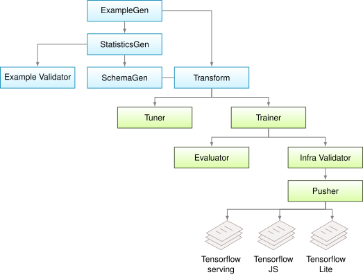](https://mlsysbook.ai/contents/core/data_engineering/9daff432776d54e821a3a38d383ac78f17ea1f27.svg "Figure 11: Data Processing Pipeline: A modular end-to-end ML pipeline, as implemented in TensorFlow extended, highlighting key stages from raw data ingestion to trained model deployment and serving. this decomposition enables independent development, versioning, and scaling of each component, improving maintainability and reproducibility of ML systems.")
Figure 11: **Data Processing Pipeline**: A modular end-to-end ML pipeline, as implemented in TensorFlow extended, highlighting key stages from raw data ingestion to trained model deployment and serving. this decomposition enables independent development, versioning, and scaling of each component, improving maintainability and reproducibility of ML systems.
Integrating these processing components, our KWS processing pipelines must handle both batch processing for training and real-time processing for inference while maintaining consistency between these modes. The pipeline design ensures that the same normalization parameters computed on training data—mean volume levels, frequency response curves, and duration statistics—are stored and applied identically during serving. This architectural decision reflects our reliability pillar: users expect consistent wake word detection regardless of when their device was manufactured or which model version it runs, requiring processing pipelines that maintain stable behavior across training iterations and deployment environments.
Effective data processing is the cornerstone of successful ML systems. By carefully cleaning, transforming, and engineering data through the lens of our four-pillar framework—quality through training-serving consistency, reliability through idempotent transformations, scalability through distributed processing, and governance through comprehensive lineage—practitioners can significantly improve the performance and reliability of their models. As the field of machine learning continues to evolve, so too do the techniques and tools for data processing, making this an exciting and dynamic area of study and practice. With systematic processing established, we now examine data labeling, which introduces human judgment into our otherwise automated pipelines while maintaining the same framework discipline across quality, reliability, scalability, and governance dimensions.
**Self-Check: Question 1.7**
1. Why is training-serving consistency crucial in data processing for ML systems?
1. It ensures that models receive the same input format during both training and serving.
2. It reduces the computational cost of data processing.
3. It allows for more diverse data transformations during training.
4. It enables faster model deployment.
2. True or False: Idempotent transformations in data processing ensure that repeated application of the same transformation yields the same result.
3. Explain how distributed processing can address scalability challenges in ML data pipelines.
4. In ML data processing, \_\_\_\_\_\_\_ ensures that transformations produce the same output for the same input, regardless of when or where they are executed.
5. In a production ML system, what is a potential consequence of failing to maintain training-serving consistency?
1. Increased model accuracy
2. Degraded model performance
3. Reduced data storage requirements
4. Simplified data governance
[See Answers →](https://mlsysbook.ai/contents/core/data_engineering/data_engineering.html#quiz-answer-sec-data-engineering-systematic-data-processing-e3d2)
Data Labeling
-------------
With systematic data processing established, data labeling emerges as a particularly complex systems challenge within the broader data engineering landscape. As training datasets grow to millions or billions of examples, the infrastructure supporting labeling operations becomes increasingly critical to system performance. Labeling represents human-in-the-loop system engineering where our four pillars guide infrastructure decisions in fundamentally different ways than in automated pipeline stages. The quality pillar manifests as ensuring label accuracy through consensus mechanisms and gold standard validation. The reliability pillar demands platform architecture that coordinates thousands of concurrent annotators without data loss or corruption. The scalability pillar drives AI assistance to amplify human judgment rather than replace it. The governance pillar requires fair compensation, bias mitigation, and ethical treatment of human contributors whose labor creates the training data enabling ML systems.
Modern machine learning systems must efficiently handle the creation, storage, and management of labels across their data pipeline. The systems architecture must support various labeling workflows while maintaining data consistency, ensuring quality, and managing computational resources effectively. These requirements compound when dealing with large-scale datasets or real-time labeling needs. The systematic challenges extend beyond just storing and managing labels—production ML systems need robust pipelines that integrate labeling workflows with data ingestion, preprocessing, and training components while maintaining high throughput and adapting to changing requirements.
### Label Types and Their System Requirements
To build effective labeling systems, we must first understand how different types of labels affect our system architecture and resource requirements. Consider a practical example: building a smart city system that needs to detect and track various objects like vehicles, pedestrians, and traffic signs from video feeds. Labels capture information about key tasks or concepts, with each label type imposing distinct storage, computation, and validation requirements.
Classification labels represent the simplest form, categorizing images with a specific tag or (in multi-label classification) tags such as labeling an image as “car” or “pedestrian.” While conceptually straightforward, a production system processing millions of video frames must efficiently store and retrieve these labels. Storage requirements are modest—a single integer or string per image—but retrieval patterns matter: training often samples random subsets while validation requires sequential access to all labels, driving different indexing strategies.
Bounding boxes extend beyond simple classification by identifying object locations, drawing a box around each object of interest. Our system now needs to track not just what objects exist, but where they are in each frame. This spatial information introduces new storage and processing challenges, especially when tracking moving objects across video frames. Each bounding box requires storing four coordinates (x, y, width, height) plus the object class, multiplying storage by 5x compared to classification. More importantly, bounding box annotation requires pixel-precise positioning that takes 10-20x longer than classification, dramatically affecting labeling throughput and cost.
Segmentation maps provide the most comprehensive information by classifying objects at the pixel level, highlighting each object in a distinct color. For our traffic monitoring system, this might mean precisely outlining each vehicle, pedestrian, and road sign. These detailed annotations significantly increase our storage and processing requirements. A segmentation mask for a 1920x1080 image requires 2 million labels (one per pixel), compared to perhaps 10 bounding boxes or a single classification label. This 100,000x storage increase and the hours required per image for manual segmentation make this approach suitable only when pixel-level precision is essential.
[](https://mlsysbook.ai/contents/core/data_engineering/images/png/cs249r_labels_new.png "Figure 12: Data Annotation Granularity: Increasing levels of detail in data labeling—from bounding boxes to pixel-level segmentation—impact both annotation cost and potential model accuracy. Fine-grained segmentation provides richer information for training but demands significantly more labeling effort and storage capacity than coarser annotations.")
Figure 12: **Data Annotation Granularity**: Increasing levels of detail in data labeling—from bounding boxes to pixel-level segmentation—impact both annotation cost and potential model accuracy. Fine-grained segmentation provides richer information for training but demands significantly more labeling effort and storage capacity than coarser annotations.
[Figure 12](https://mlsysbook.ai/contents/core/data_engineering/data_engineering.html#fig-labels)
illustrates these common label types and their increasing complexity. Given these increasing complexity levels, the choice of label format depends heavily on our system requirements and resource constraints ([Johnson-Roberson et al. 2017](https://mlsysbook.ai/contents/core/data_engineering/data_engineering.html#ref-10.1109/ICRA.2017.7989092)
). While classification labels might suffice for simple traffic counting, autonomous vehicles need detailed segmentation maps to make precise navigation decisions. Leading autonomous vehicle companies often maintain hybrid systems that store multiple label types for the same data, allowing flexible use across different applications. A single camera frame might have classification labels (scene type: highway, urban, rural), bounding boxes (vehicles and pedestrians for obstacle detection), and segmentation masks (road surface for path planning), with each label type serving distinct downstream models.
Johnson-Roberson, Matthew, Charles Barto, Rounak Mehta, Sharath Nittur Sridhar, Karl Rosaen, and Ram Vasudevan. 2017. “Driving in the Matrix: Can Virtual Worlds Replace Human-Generated Annotations for Real World Tasks?” In _2017 IEEE International Conference on Robotics and Automation (ICRA)_, 746–53. Singapore, Singapore: IEEE. [https://doi.org/10.1109/icra.2017.7989092](https://doi.org/10.1109/icra.2017.7989092)
.
Ardila, Rosana, Megan Branson, Kelly Davis, Michael Kohler, Josh Meyer, Michael Henretty, Reuben Morais, Lindsay Saunders, Francis Tyers, and Gregor Weber. 2020. “Common Voice: A Massively-Multilingual Speech Corpus.” In _Proceedings of the Twelfth Language Resources and Evaluation Conference_, 4218–22. Marseille, France: European Language Resources Association. [https://aclanthology.org/2020.lrec-1.520](https://aclanthology.org/2020.lrec-1.520)
.
Extending beyond these basic label types, production systems must also handle rich metadata essential for maintaining data quality and debugging model behavior. The Common Voice dataset ([Ardila et al. 2020](https://mlsysbook.ai/contents/core/data_engineering/data_engineering.html#ref-ardila2020common)
) exemplifies sophisticated metadata management in speech recognition: tracking speaker demographics for model fairness, recording quality metrics for data filtering, validation status for label reliability, and language information for multilingual support. If our traffic monitoring system performs poorly in rainy conditions, weather condition metadata during data collection helps identify and address the issue. Modern labeling platforms have built sophisticated metadata management systems that efficiently index and query this metadata alongside primary labels, enabling filtering during training data selection and post-hoc analysis when model failures are discovered.
These metadata requirements demonstrate how label type choice cascades through entire system design. A system built for simple classification labels would need significant modifications to handle segmentation maps efficiently. The infrastructure must optimize storage systems for the chosen label format, implement efficient data retrieval patterns for training, maintain quality control pipelines for validation as established in [Section 1.7.1](https://mlsysbook.ai/contents/core/data_engineering/data_engineering.html#sec-data-engineering-ensuring-trainingserving-consistency-f3b7)
, and manage version control for label updates. When labels are corrected or refined, the system must track which model versions used which label versions, enabling correlation between label quality improvements and model performance gains.
### Achieving Label Accuracy and Consensus
In the labeling domain, quality takes on unique challenges. The quality pillar here focuses on ensuring label accuracy despite the inherent subjectivity and ambiguity in many labeling tasks. Even with clear guidelines and careful system design, some fraction of labels will inevitably be incorrect Thyagarajan et al. ([2022](https://mlsysbook.ai/contents/core/data_engineering/data_engineering.html#ref-thyagarajan2023multilabel)
). The challenge is not eliminating labeling errors entirely—an impossible goal—but systematically measuring and managing error rates to keep them within bounds that don’t degrade model performance.
Thyagarajan, Aditya, Elías Snorrason, Curtis G. Northcutt, and Jonas Mueller 0001. 2022. “Identifying Incorrect Annotations in Multi-Label Classification Data.” _CoRR_. [https://doi.org/10.48550/ARXIV.2211.13895](https://doi.org/10.48550/ARXIV.2211.13895)
.
As [Figure 13](https://mlsysbook.ai/contents/core/data_engineering/data_engineering.html#fig-hard-labels)
illustrates, labeling failures arise from two distinct sources requiring different engineering responses. Some errors stem from data quality issues where the underlying data is genuinely ambiguous or corrupted—like the blurred frog image where even expert annotators cannot determine the species with certainty. Other errors require deep domain expertise where the correct label is determinable but only by experts with specialized knowledge, as with the black stork identification. These different failure modes drive architectural decisions about annotator qualification, task routing, and consensus mechanisms.
[](https://mlsysbook.ai/contents/core/data_engineering/images/png/label-errors-examples_new.png "Figure 13: Labeling Ambiguity: How subjective or difficult examples, such as blurry images or rare species, can introduce errors during data labeling, highlighting the need for careful quality control and potentially expert annotation. Source: [@northcutt2021pervasive].")
Figure 13: **Labeling Ambiguity**: How subjective or difficult examples, such as blurry images or rare species, can introduce errors during data labeling, highlighting the need for careful quality control and potentially expert annotation. Source: ([Northcutt, Athalye, and Mueller 2021](https://mlsysbook.ai/contents/core/data_engineering/data_engineering.html#ref-northcutt2021pervasive)
).
Northcutt, Curtis G, Anish Athalye, and Jonas Mueller. 2021. “Pervasive Label Errors in Test Sets Destabilize Machine Learning Benchmarks.” _arXiv_. https://doi.org/[https://doi.org/10.48550/arXiv.2103.14749 arXiv-issued DOI via DataCite](https://doi.org/10.48550/arXiv.2103.14749%20arXiv-issued%20DOI%20via%20DataCite)
.
Given these fundamental quality challenges, production ML systems implement multiple layers of quality control. Systematic quality checks continuously monitor the labeling pipeline through random sampling of labeled data for expert review and statistical methods to flag potential errors. The infrastructure must efficiently process these checks across millions of examples without creating bottlenecks. Sampling strategies typically validate 1-10% of labels, balancing detection sensitivity against review costs. Higher-risk applications like medical diagnosis or autonomous vehicles may validate 100% of labels through multiple independent reviews, while lower-stakes applications like product recommendations may validate only 1% through spot checks.
Beyond random sampling approaches, collecting multiple labels per data point, often referred to as “consensus labeling,” can help identify controversial or ambiguous cases. Professional labeling companies have developed sophisticated infrastructure for this process. For example, [Labelbox](https://labelbox.com/)
has consensus tools that track inter-annotator agreement rates and automatically route controversial cases for expert review. [Scale AI](https://scale.com/)
implements tiered quality control, where experienced annotators verify the work of newer team members. The consensus infrastructure typically collects 3-5 labels per example, computing inter-annotator agreement using metrics like Fleiss’ kappa which measures agreement beyond what would occur by chance. Examples with low agreement (kappa below 0.4) route to expert review rather than forcing consensus from genuinely ambiguous cases.
The consensus approach reflects an economic trade-off essential for scalable systems. Expert review costs 10-50x more per example than crowdsourced labeling, but forcing agreement on ambiguous examples through majority voting of non-experts produces systematically biased labels. By routing only genuinely ambiguous cases to experts—often 5-15% of examples identified through low inter-annotator agreement—systems balance cost against quality. This tiered approach enables processing millions of examples economically while maintaining quality standards through targeted expert intervention.
While technical infrastructure provides the foundation for quality control, successful labeling systems must also consider human factors. When working with annotators, organizations need robust systems for training and guidance. This includes good documentation with clear examples of correct labeling, visual demonstrations of edge cases and how to handle them, regular feedback mechanisms showing annotators their accuracy on gold standard examples, and calibration sessions where annotators discuss ambiguous cases to develop shared understanding. For complex or domain-specific tasks, the system might implement tiered access levels, routing challenging cases to annotators with appropriate expertise based on their demonstrated accuracy on similar examples.
Quality monitoring generates substantial data that must be efficiently processed and tracked. Organizations typically monitor inter-annotator agreement rates (tracking whether multiple annotators agree on the same example), label confidence scores (how certain annotators are about their labels), time spent per annotation (both too fast suggesting careless work and too slow suggesting confusion), error patterns and types (systematic biases or misunderstandings), annotator performance metrics (accuracy on gold standard examples), and bias indicators (whether certain annotator demographics systematically label differently). These metrics must be computed and updated efficiently across millions of examples, often requiring dedicated analytics pipelines that process labeling data in near real-time to catch quality issues before they affect large volumes of data.
### Building Reliable Labeling Platforms
Moving from label quality to system reliability, we examine how platform architecture supports consistent operations. While quality focuses on label accuracy, reliability ensures the platform architecture itself operates consistently at scale. Scaling labeling from hundreds to millions of examples while maintaining quality requires understanding how production labeling systems separate concerns across multiple architectural components. The fundamental challenge is that labeling represents a human-in-the-loop workflow where system performance depends not just on infrastructure but on managing human attention, expertise, and consistency.
At the foundation sits a durable task queue that stores labeling tasks persistently, ensuring no work gets lost when systems restart or annotators disconnect. Most production systems use message queues like Apache Kafka or RabbitMQ rather than databases for this purpose, since message queues provide natural ordering, parallel consumption, and replay capabilities that databases don’t easily support. Each task carries metadata beyond just the data to be labeled: what type of task it is (classification, bounding boxes, segmentation), what expertise level it requires, how urgent it is, and any context needed for accurate labeling—perhaps related examples or relevant documentation.
The assignment service that routes tasks to annotators implements matching logic that’s more sophisticated than simple round-robin distribution. Medical image labeling systems route chest X-rays specifically to annotators who have demonstrated radiology expertise, measured by their agreement with expert labels on gold standard examples. But expertise matching alone isn’t sufficient—annotators who see only chest images or only a specific pathology can develop blind spots, performing well on familiar examples but poorly on less common cases. Production systems therefore constraint assignment to ensure no annotator receives more than 30% of their tasks from a single category, maintaining breadth of exposure that prevents overspecialization from degrading quality on less-familiar examples.
When tasks require multiple annotations to ensure quality, the consensus engine determines both when sufficient labels have been collected and how to aggregate potentially conflicting opinions. Simple majority voting works for clear-cut classification tasks where most annotators naturally agree: identifying whether an image contains a car rarely produces disagreement. But more subjective tasks like sentiment analysis or identifying nuanced image attributes produce legitimate disagreement between thoughtful annotators. A common pattern addresses this by collecting 3-5 labels per example, computing inter-annotator agreement using Fleiss’ kappa (which measures agreement beyond chance), and routing examples with low agreement—typically kappa below 0.4—to expert review rather than forcing consensus from genuinely ambiguous cases.
This tiered approach reflects a fundamental economic trade-off that shapes platform architecture. Expert review costs 10-50x more per example than crowdsourced labeling, but forcing agreement on ambiguous examples through majority voting of non-experts produces systematically biased labels—biased toward easier-to-label patterns that may not reflect the complexity important for model robustness. By routing only genuinely ambiguous cases to experts—often 5-15% of examples identified through low inter-annotator agreement—systems balance cost against quality. The platform must implement this routing logic efficiently, tracking which examples need expert review and ensuring they’re delivered to appropriately qualified annotators without creating bottlenecks.
Maintaining quality at scale requires continuous measurement through gold standard injection. The system periodically inserts examples with known correct labels into the task stream without revealing which examples are gold standard. This enables computing per-annotator accuracy without the Hawthorne effect where measurement changes behavior—annotators can’t “try harder” on gold standard examples if they don’t know which ones they are. Annotators consistently scoring below 85% on gold standards receive additional training materials, more detailed guidelines, or removal from the pool if performance doesn’t improve. Beyond simple accuracy, systems track quality across multiple dimensions: agreement with peer annotators on the same tasks (detecting systematic disagreement suggesting misunderstanding of guidelines), time per task (both too fast suggesting careless work and too slow suggesting confusion), and consistency where the same annotator sees similar examples shown days apart to measure whether they apply labels reliably over time.
The performance requirements of these systems become demanding at scale. A labeling platform processing 10,000 annotations per hour must balance latency requirements against database write capacity. Writing each annotation immediately to a persistent database like PostgreSQL for durability would require 2-3 writes per second, well within database capacity. But task serving—delivering new tasks to 100,000 concurrent annotators requesting work—requires subsecond response times that databases struggle to provide when serving requests fan out across many annotators. Production systems therefore maintain a two-tier storage architecture: Redis caches active tasks enabling sub-100ms task assignment latency, while annotations batch write to PostgreSQL every 100 annotations (typically every 30-60 seconds), providing durability without overwhelming the database with small writes.
Horizontal scaling of these systems requires careful data partitioning. Tasks shard by task\_id enabling independent task queue scaling, annotator performance metrics shard by annotator\_id for fast lookup during assignment decisions, and aggregated labels shard by example\_id for efficient retrieval during model training. This partitioning strategy enables systems handling millions of tasks daily to support 100,000+ concurrent annotators with median task assignment latency under 50ms, proving that human-in-the-loop systems can scale to match fully automated pipelines when properly architected.
Beyond these architectural considerations, understanding the economics of labeling operations reveals why scalability through AI assistance becomes essential. Data labeling represents one of ML systems’ largest hidden costs, yet it is frequently overlooked in project planning that focuses primarily on compute infrastructure and model training expenses. While teams carefully optimize GPU utilization and track training costs measured in dollars per hour, labeling expenses measured in dollars per example often receive less scrutiny despite frequently exceeding compute costs by orders of magnitude. Understanding the full economic model reveals why scalability through AI assistance becomes not just beneficial but economically necessary as ML systems mature and data requirements grow to millions or billions of labeled examples, which **[Chapter 13: ML Operations](https://mlsysbook.ai/contents/core/ops/ops.html#sec-ml-operations)
** examines where operational costs compound across the ML lifecycle.
The cost structure of labeling operations follows a multiplicative model capturing both direct annotation costs and quality control overhead:
\\\[\\text{Total Cost} = N \\times \\text{Cost}\_{\\text{label}} \\times (1 + R\_{\\text{review}}) \\times (1 + R\_{\\text{rework}})\\\]
where \\(N\\) represents the number of examples, \\(\\text{Cost}\_{\\text{label}}\\) is the base cost per label, \\(R\_{\\text{review}}\\) is the fraction requiring expert review (typically 0.05-0.15), and \\(R\_{\\text{rework}}\\) accounts for labels requiring correction (typically 0.10-0.30). This equation reveals how quality requirements compound costs: a dataset requiring 1 million labels at $0.10 per label with 10% expert review (costing 5x more, or $0.50) and 20% rework reaches $138,000, not the $100,000 that naive calculation suggests. For comparison, training a ResNet-50 model on this data might cost only $50 for compute—nearly 3,000x less than labeling, demonstrating why labeling economics dominate total system costs yet receive insufficient attention during planning phases.
The cost per label varies dramatically by task complexity and required expertise. Simple image classification ranges from $0.01-0.05 per label when crowdsourced but rises to $0.50-2.00 when requiring expert verification. Bounding boxes cost $0.05-0.20 per box for straightforward cases but $1.00-5.00 for dense scenes with many overlapping objects. Semantic segmentation can reach $5-50 per image depending on precision requirements and object boundaries. Medical image annotation by radiologists costs $50-200 per study. When a computer vision system requires 10 million labeled images, the difference between $0.02 and $0.05 per label represents $300,000 in project costs—often more than the entire infrastructure budget yet frequently discovered only after labeling begins.
### Scaling with AI-Assisted Labeling
As labeling demands grow exponentially with modern ML systems, scalability becomes critical. The scalability pillar drives AI assistance as a force multiplier for human labeling rather than a replacement. Manual annotation alone cannot keep pace with modern ML systems’ data needs, while fully automated labeling lacks the nuanced judgment that humans provide. AI-assisted labeling finds the sweet spot: using automation to handle clear cases and accelerate annotation while preserving human judgment for ambiguous or high-stakes decisions. As illustrated in [Figure 14](https://mlsysbook.ai/contents/core/data_engineering/data_engineering.html#fig-weak-supervision)
, AI assistance offers several paths to scale labeling operations, each requiring careful system design to balance speed, quality, and resource usage.
[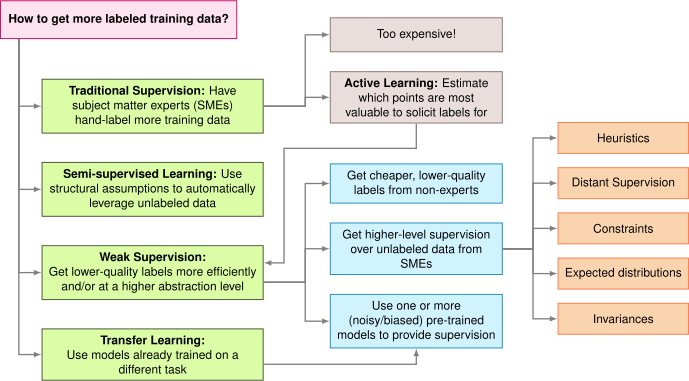](https://mlsysbook.ai/contents/core/data_engineering/a271bd786f6723a93e5e1b3dff59701d8362b9f2.svg "Figure 14: AI-Augmented Labeling: Programmatic labeling, distant supervision, and active learning scale data annotation by trading potential labeling errors for increased throughput, necessitating careful system design to balance labeling speed, cost, and model quality. These strategies enable machine learning systems to overcome limitations imposed by manual annotation alone, facilitating deployment in data-scarce environments. Source: Stanford AI Lab.")
Figure 14: **AI-Augmented Labeling**: Programmatic labeling, distant supervision, and active learning scale data annotation by trading potential labeling errors for increased throughput, necessitating careful system design to balance labeling speed, cost, and model quality. These strategies enable machine learning systems to overcome limitations imposed by manual annotation alone, facilitating deployment in data-scarce environments. Source: Stanford AI Lab.
Modern AI-assisted labeling typically employs a combination of approaches working together in the pipeline. Pre-annotation involves using AI models to generate preliminary labels for a dataset, which humans can then review and correct. Major labeling platforms have made significant investments in this technology. [Snorkel AI](https://snorkel.ai/)
uses programmatic labeling ([Ratner et al. 2018](https://mlsysbook.ai/contents/core/data_engineering/data_engineering.html#ref-ratner2018snorkel)
) to automatically generate initial labels at scale through rule-based heuristics and weak supervision signals. Scale AI deploys pre-trained models to accelerate annotation in specific domains like autonomous driving, where object detection models pre-label vehicles and pedestrians that humans then verify and refine. Companies like [SuperAnnotate](https://www.superannotate.com/)
provide automated pre-labeling tools that can reduce manual effort by 50-80% for computer vision tasks. This method, which often employs semi-supervised learning techniques ([Chapelle, Scholkopf, and Zien 2009](https://mlsysbook.ai/contents/core/data_engineering/data_engineering.html#ref-chapelle2009semisupervised)
), can save significant time, especially for extremely large datasets.
Ratner, Alex, Braden Hancock, Jared Dunnmon, Roger Goldman, and Christopher Ré. 2018. “Snorkel MeTaL: Weak Supervision for Multi-Task Learning.” In _Proceedings of the Second Workshop on Data Management for End-to-End Machine Learning_, 1–4. ACM. [https://doi.org/10.1145/3209889.3209898](https://doi.org/10.1145/3209889.3209898)
.
Chapelle, O., B. Scholkopf, and A. Zien Eds. 2009. “Semi-Supervised Learning (Chapelle, o. Et Al., Eds.; 2006) \[Book Reviews\].” _IEEE Transactions on Neural Networks_ 20 (3): 542–42. [https://doi.org/10.1109/tnn.2009.2015974](https://doi.org/10.1109/tnn.2009.2015974)
.
The emergence of Large Language Models (LLMs) like ChatGPT has further transformed labeling pipelines. Beyond simple classification, LLMs can generate rich text descriptions, create labeling guidelines from examples, and even explain their reasoning for label assignments. For instance, content moderation systems use LLMs to perform initial content classification and generate explanations for policy violations that human reviewers can validate. However, integrating LLMs introduces new system challenges around inference costs (API calls can cost $0.01-$1 per example depending on complexity), rate limiting (cloud APIs typically limit to 100-10,000 requests per minute), and output validation (LLMs occasionally produce confident but incorrect labels requiring systematic validation). Many organizations adopt a tiered approach, using smaller specialized models for routine cases while reserving larger LLMs for complex scenarios requiring nuanced judgment or rare domain expertise.
Methods such as active learning complement these approaches by intelligently prioritizing which examples need human attention ([Coleman et al. 2022](https://mlsysbook.ai/contents/core/data_engineering/data_engineering.html#ref-coleman2022similarity)
). These systems continuously analyze model uncertainty to identify valuable labeling candidates. Rather than labeling a random sample of unlabeled data, active learning selects examples where the current model is most uncertain or where labels would most improve model performance. The infrastructure must efficiently compute uncertainty metrics (often prediction entropy or disagreement between ensemble models), maintain task queues ordered by informativeness, and adapt prioritization strategies based on incoming labels. Consider a medical imaging system: active learning might identify unusual pathologies for expert review while handling routine cases through pre-annotation that experts merely verify. This approach can reduce required annotations by 50-90% compared to random sampling, though it requires careful engineering to prevent feedback loops where the model’s uncertainty biases which data gets labeled.
Coleman, Cody, Edward Chou, Julian Katz-Samuels, Sean Culatana, Peter Bailis, Alexander C. Berg, Robert Nowak, Roshan Sumbaly, Matei Zaharia, and I. Zeki Yalniz. 2022. “Similarity Search for Efficient Active Learning and Search of Rare Concepts.” _Proceedings of the AAAI Conference on Artificial Intelligence_ 36 (6): 6402–10. [https://doi.org/10.1609/aaai.v36i6.20591](https://doi.org/10.1609/aaai.v36i6.20591)
.
Quality control becomes increasingly crucial as these AI components interact. The system must monitor both AI and human performance through systematic metrics. Model confidence calibration matters: if the AI says it’s 95% confident but is actually only 75% accurate at that confidence level, pre-annotations mislead human reviewers. Human-AI agreement rates reveal whether AI assistance helps or hinders: when humans frequently override AI suggestions, the pre-annotations may be introducing bias rather than accelerating work. These metrics require careful instrumentation throughout the labeling pipeline, tracking not just final labels but the interaction between human and AI at each stage.
In safety-critical domains like self-driving cars, these systems must maintain particularly rigorous standards while processing massive streams of sensor data. Waymo’s labeling infrastructure reportedly processes millions of sensor frames daily, using AI pre-annotation to label common objects (vehicles, pedestrians, traffic signs) while routing unusual scenarios (construction zones, emergency vehicles, unusual road conditions) to human experts. The system must maintain real-time performance despite this scale, using distributed architectures where pre-annotation runs on GPU clusters while human review scales horizontally across thousands of annotators, with careful load balancing ensuring neither component becomes a bottleneck.
Real-world deployments demonstrate these principles at scale in diverse domains. Medical imaging systems ([Krishnan, Rajpurkar, and Topol 2022](https://mlsysbook.ai/contents/core/data_engineering/data_engineering.html#ref-krishnan2022selfsupervised)
) combine pre-annotation for common conditions (identifying normal tissue, standard anatomical structures) with active learning for unusual cases (rare pathologies, ambiguous findings), all while maintaining strict patient privacy through secure annotation platforms with comprehensive audit trails. Self-driving vehicle systems coordinate multiple AI models to label diverse sensor data: one model pre-labels camera images, another handles lidar point clouds, a third processes radar data, with fusion logic combining predictions before human review. Social media platforms process millions of items hourly using tiered approaches where simpler models handle clear violations (spam, obvious hate speech) while complex content routes to more sophisticated models or human reviewers when initial classification is uncertain.
Krishnan, Rayan, Pranav Rajpurkar, and Eric J. Topol. 2022. “Self-Supervised Learning in Medicine and Healthcare.” _Nature Biomedical Engineering_ 6 (12): 1346–52. [https://doi.org/10.1038/s41551-022-00914-1](https://doi.org/10.1038/s41551-022-00914-1)
.
### Ensuring Ethical and Fair Labeling
Unlike previous sections where governance focused on data and processes, labeling governance centers on human welfare. The governance pillar here addresses ethical treatment of human contributors, bias mitigation, and fair compensation—challenges that manifest distinctly from governance in automated pipeline stages because human welfare is directly at stake. While governance in processing focuses on data lineage and compliance, governance in labeling requires ensuring that the humans creating training data are treated ethically, compensated fairly, and protected from harm.
However, alongside these compelling advantages of crowdsourcing, the challenges highlighted by real-world examples demonstrate why governance cannot be an afterthought. The issue of fair compensation and ethical data sourcing was brought into sharp focus during the development of large-scale AI systems like OpenAI’s ChatGPT. Reports revealed that [OpenAI outsourced data annotation tasks to workers in Kenya](https://time.com/6247678/openai-chatgpt-kenya-workers/)
, employing them to moderate content and identify harmful or inappropriate material that the model might generate. This involved reviewing and labeling distressing content, such as graphic violence and explicit material, to train the AI in recognizing and avoiding such outputs. While this approach enabled OpenAI to improve the safety and utility of ChatGPT, significant ethical concerns arose around the working conditions, the nature of the tasks, and the compensation provided to Kenyan workers.
Many of the contributors were reportedly paid as little as $1.32 per hour for reviewing and labeling highly traumatic material. The emotional toll of such work, coupled with low wages, raised serious questions about the fairness and transparency of the crowdsourcing process. This controversy highlights a critical gap in ethical crowdsourcing practices. The workers, often from economically disadvantaged regions, were not adequately supported to cope with the psychological impact of their tasks. The lack of mental health resources and insufficient compensation underscored the power imbalances that can emerge when outsourcing data annotation tasks to lower-income regions.
Unfortunately, the challenges highlighted by the ChatGPT Kenya controversy are not unique to OpenAI. Many organizations that rely on crowdsourcing for data annotation face similar issues. As machine learning systems grow more complex and require larger datasets, the demand for annotated data will continue to increase. This shows the need for industry-wide standards and best practices to ensure ethical data sourcing. Fair compensation means paying at least local minimum wages, ideally benchmarked against comparable work in workers’ regions—not just the legally minimum but what would be considered fair for skilled work requiring sustained attention. For sensitive content moderation, this often means premium pay reflecting psychological burden, sometimes 2-3x base rates.
Worker wellbeing requires providing mental health resources for those dealing with sensitive content. Organizations like [Scale AI](https://scale.com/)
have implemented structured support including: limiting exposure to traumatic content (rotating annotators through different content types, capping hours per day on disturbing material), providing access to counseling services at no cost to workers, and offering immediate support channels when annotators encounter particularly disturbing content. These measures add operational cost but are essential for ethical operations. Transparency demands clear communication about task purposes, how contributions will be used, what kind of content workers might encounter, and worker rights including ability to skip tasks that cause distress.
Beyond working conditions, bias in data labeling represents another critical governance concern. Annotators bring their own cultural, personal, and professional biases to the labeling process, which can be reflected in the resulting dataset. For example, Wang et al. ([2019](https://mlsysbook.ai/contents/core/data_engineering/data_engineering.html#ref-wang2019balanced)
) found that image datasets labeled predominantly by annotators from one geographic region showed biases in object recognition tasks, performing poorly on images from other regions. This highlights the need for diverse annotator pools where demographic diversity among annotators helps counteract individual biases, though it doesn’t eliminate them. Regular bias audits examining whether label distributions differ systematically across annotator demographics, monitoring for patterns suggesting systematic bias (all images from certain regions receiving lower quality scores), and addressing identified biases through additional training or guideline refinement ensure labels support fair model behavior.
Wang, Tianlu, Jieyu Zhao, Mark Yatskar, Kai-Wei Chang, and Vicente Ordonez. 2019. “Balanced Datasets Are Not Enough: Estimating and Mitigating Gender Bias in Deep Image Representations.” In _2019 IEEE/CVF International Conference on Computer Vision (ICCV)_, 5309–18. IEEE. [https://doi.org/10.1109/iccv.2019.00541](https://doi.org/10.1109/iccv.2019.00541)
.
25 Chapter 13 covers Security and Privacy in depth, building upon the data governance foundations established here to address comprehensive protection strategies for ML systems.
Data privacy and ethical considerations also pose challenges in data labeling. Leading data labeling companies have developed specialized solutions for these challenges. Scale AI, for instance, maintains dedicated teams and secure infrastructure for handling sensitive data in healthcare and finance, with HIPAA-compliant annotation platforms and strict data access controls. Appen implements strict data access controls and anonymization protocols, ensuring annotators never see personally identifiable information when unnecessary. Labelbox offers private cloud deployments for organizations with strict security requirements, enabling annotation without data leaving organizational boundaries. These privacy-preserving techniques connect directly to the security considerations we explore in future chapters[25](https://mlsysbook.ai/contents/core/data_engineering/data_engineering.html#fn25)
, where comprehensive approaches to protecting sensitive data throughout the ML lifecycle are examined.
Beyond privacy and working conditions, the dynamic nature of real-world data presents another limitation. Labels that are accurate at the time of annotation may become outdated or irrelevant as the underlying distribution of data changes over time. This concept, known as concept drift, necessitates ongoing labeling efforts and periodic re-evaluation of existing labels. Governance frameworks must account for label versioning (tracking when labels were created and by whom), re-annotation policies (systematically re-labeling data when concepts evolve), and retirement strategies (identifying when old labels should be deprecated rather than used for training).
Finally, the limitations of current labeling approaches become apparent when dealing with edge cases or rare events. In many real-world applications, it’s the unusual or rare instances that are often most critical (e.g., rare diseases in medical diagnosis, or unusual road conditions in autonomous driving). However, these cases are, by definition, underrepresented in most datasets and may be overlooked or mislabeled in large-scale annotation efforts. Governance requires explicit strategies for handling rare events: targeted collection campaigns for underrepresented scenarios, expert review requirements for rare cases, and systematic tracking ensuring rare events receive appropriate attention despite their low frequency.
This case emphasizes the importance of considering the human labor behind AI systems. While crowdsourcing offers scalability and diversity, it also brings ethical responsibilities that cannot be overlooked. Organizations must prioritize the well-being and fair treatment of contributors as they build the datasets that drive AI innovation. Governance in labeling ultimately means recognizing that training data isn’t just bits and bytes but the product of human labor deserving respect, fair compensation, and ethical treatment.
### Case Study: Automated Labeling in KWS Systems
Continuing our KWS case study through the labeling stage—having established systematic problem definition ([Section 1.3.3](https://mlsysbook.ai/contents/core/data_engineering/data_engineering.html#sec-data-engineering-framework-application-keyword-spotting-case-study-21ff)
), diverse data collection strategies that address quality and coverage requirements, ingestion patterns handling both batch and streaming workflows, and processing pipelines ensuring training-serving consistency—we now confront a challenge unique to speech systems at scale. Generating millions of labeled wake word samples without proportional human annotation cost requires moving beyond the manual and crowdsourced approaches we examined earlier. The Multilingual Spoken Words Corpus (MSWC) ([Mazumder et al. 2021](https://mlsysbook.ai/contents/core/data_engineering/data_engineering.html#ref-mazumder2021multilingual)
) demonstrates how automated labeling addresses this challenge through its innovative approach to generating labeled wake word data, containing over 23.4 million one-second spoken examples across 340,000 keywords in 50 different languages.
Mazumder, Mark, Sharad Chitlangia, Colby Banbury, Yiping Kang, Juan Manuel Ciro, Keith Achorn, Daniel Galvez, et al. 2021. “Multilingual Spoken Words Corpus.” In _Thirty-Fifth Conference on Neural Information Processing Systems Datasets and Benchmarks Track (Round 2)_.
This scale directly reflects our framework pillars in practice. Achieving our quality target of 98% accuracy across diverse environments requires millions of training examples covering acoustic variations we identified during problem definition. Reliability demands representation across varied acoustic conditions—different background noises, speaking styles, and recording environments. Scalability necessitates automation rather than manual labeling because 23.4 million examples would require approximately 2,600 person-years of effort at even 10 seconds per label, making manual annotation economically infeasible. Governance requirements mandate transparent sourcing and language diversity, ensuring voice-activated technology serves speakers of many languages rather than concentrating on only the most commercially valuable markets.
As illustrated in [Figure 15](https://mlsysbook.ai/contents/core/data_engineering/data_engineering.html#fig-mswc)
, this automated system begins with paired sentence audio recordings and corresponding transcriptions from projects like [Common Voice](https://commonvoice.mozilla.org/en)
or multilingual captioned content platforms. The system processes these inputs through forced alignment[26](https://mlsysbook.ai/contents/core/data_engineering/data_engineering.html#fn26)
—a computational technique that identifies precise word boundaries within continuous speech by analyzing both audio and transcription simultaneously.
26 **Forced alignment**: An automated speech processing technique that determines precise time boundaries for words within continuous speech by aligning audio with its transcription using acoustic models. The system computes optimal alignment paths through dynamic programming, matching phonetic sequences to audio frames, enabling extraction of individual words with millisecond precision for training data generation. Tools such as the Montreal Forced Aligner ([McAuliffe et al. 2017](https://mlsysbook.ai/contents/core/data_engineering/data_engineering.html#ref-mcauliffe17_interspeech)
) map timing relationships between written words and spoken sounds at millisecond-level precision, enabling extraction of individual keywords as one-second segments suitable for KWS training.
McAuliffe, Michael, Michaela Socolof, Sarah Mihuc, Michael Wagner, and Morgan Sonderegger. 2017. “Montreal Forced Aligner: Trainable Text-Speech Alignment Using Kaldi.” In _Interspeech 2017_, 498–502. ISCA. [https://doi.org/10.21437/interspeech.2017-1386](https://doi.org/10.21437/interspeech.2017-1386)
.
[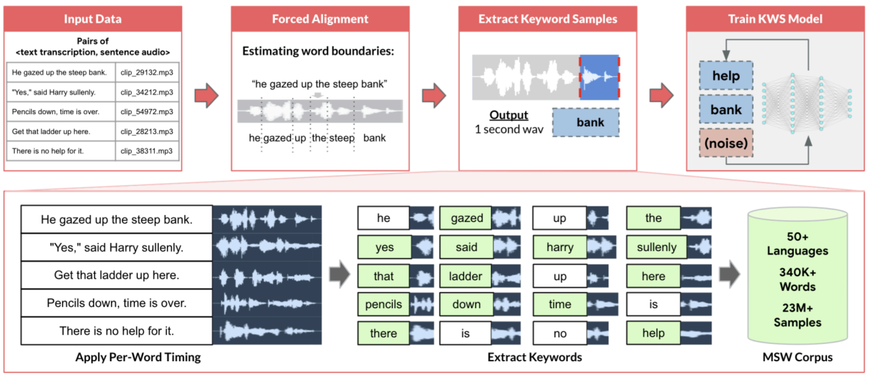](https://mlsysbook.ai/contents/core/data_engineering/images/png/data_engineering_kws2.png "Figure 15: Multilingual Data Preparation: Forced alignment and segmentation transform paired audio-text data into labeled one-second segments, creating a large-scale corpus for training keyword spotting models across 50+ languages. This automated process enables scalable development of KWS systems by efficiently generating training examples from readily available speech resources like common voice and multilingual captioned content.")
Figure 15: **Multilingual Data Preparation**: Forced alignment and segmentation transform paired audio-text data into labeled one-second segments, creating a large-scale corpus for training keyword spotting models across 50+ languages. This automated process enables scalable development of KWS systems by efficiently generating training examples from readily available speech resources like common voice and multilingual captioned content.
Building on these precise timing markers, the extraction system generates clean keyword samples while handling engineering challenges our problem definition anticipated: background noise interfering with word boundaries, speakers stretching or compressing words unexpectedly beyond our target 500-800 millisecond duration, and longer words exceeding the one-second boundary. MSWC provides automated quality assessment that analyzes audio characteristics to identify potential issues with recording quality, speech clarity, or background noise—crucial for maintaining consistent standards across 23 million samples without the manual review expenses that would make this scale prohibitive.
Modern voice assistant developers often build upon this automated labeling foundation. While automated corpora may not contain the specific wake words a product requires, they provide starting points for KWS prototyping, particularly in underserved languages where commercial datasets don’t exist. Production systems typically layer targeted human recording and verification for challenging cases—unusual accents, rare words, or difficult acoustic environments that automated systems struggle with—requiring infrastructure that gracefully coordinates between automated processing and human expertise. This demonstrates how the four pillars guide integration: quality through targeted human verification, reliability through automated consistency, scalability through forced alignment, and governance through transparent sourcing and multilingual coverage.
The sophisticated orchestration of forced alignment, extraction, and quality control demonstrates how thoughtful data engineering directly impacts production machine learning systems. When a voice assistant responds to its wake word, it draws upon this labeling infrastructure combined with the collection strategies, pipeline architectures, and processing transformations we’ve examined throughout this chapter. Storage architecture, which we turn to next, completes this picture by determining how these carefully labeled datasets are organized, accessed, and maintained throughout the ML lifecycle, enabling efficient training iterations and reliable serving at scale.
**Self-Check: Question 1.8**
1. Which of the following label types requires the most storage and processing resources in a data labeling system?
1. Segmentation maps
2. Bounding boxes
3. Classification labels
4. Metadata labels
2. Explain how the four pillars (quality, reliability, scalability, and governance) guide infrastructure decisions in data labeling systems.
3. In a production ML system, what is a potential trade-off when using consensus labeling to ensure quality?
1. Increased labeling speed
2. Reduced need for human annotators
3. Higher cost due to expert reviews
4. Simplified system architecture
4. True or False: In data labeling systems, using AI assistance can completely replace the need for human annotators.
5. Consider a scenario where a labeling system must handle both routine and rare cases in a medical imaging application. How might the system be designed to efficiently manage these different types of cases?
[See Answers →](https://mlsysbook.ai/contents/core/data_engineering/data_engineering.html#quiz-answer-sec-data-engineering-data-labeling-95e7)
Strategic Storage Architecture
------------------------------
After establishing systematic processing pipelines that transform raw data into ML-ready formats, we must design storage architectures that support the entire ML lifecycle while maintaining our four-pillar framework. Storage decisions determine how effectively we can maintain data quality over time, ensure reliable access under varying loads, scale to handle growing data volumes, and implement governance controls. The seemingly straightforward question of “where should we store this data” actually encompasses complex trade-offs between access patterns, cost constraints, consistency requirements, and performance characteristics that fundamentally shape how ML systems operate.
ML storage requirements differ fundamentally from transactional systems that power traditional applications. Rather than optimizing for frequent small writes and point lookups that characterize e-commerce or banking systems, ML workloads prioritize high-throughput sequential reads over frequent writes, large-scale scans over row-level updates, and schema flexibility over rigid structures. A database serving an e-commerce application performs well with millions of individual product lookups per second, but an ML training job that needs to scan that entire product catalog repeatedly across training epochs requires completely different storage optimization. This section examines how to match storage architectures to ML workload characteristics, comparing databases, data warehouses, and data lakes before exploring specialized ML infrastructure like feature stores and examining how storage requirements evolve across the ML lifecycle.
### ML Storage Systems Architecture Options
Storage system selection represents a critical architectural decision that affects all aspects of the ML lifecycle from development through production operations. The choice between databases, data warehouses, and data lakes determines not just where data resides but how quickly teams can iterate during development, how models access training data, and how serving systems retrieve features in production. Understanding these trade-offs requires examining both fundamental storage characteristics and the specific access patterns of different ML tasks.
The key insight is that different ML workloads have fundamentally different storage requirements based on their access patterns and latency needs:
* **Databases (OLTP)**: Excel for online feature serving where you need low-latency, random access to individual records. A recommendation system looking up a user’s profile during real-time inference exemplifies this pattern: millisecond lookups of specific user features (age, location, preferences) to generate personalized recommendations.
* **Data warehouses (OLAP)**: Optimize for model training on structured data where you need high-throughput, sequential scans over large, clean tables. Training a fraud detection model that processes millions of transactions with hundreds of features per transaction benefits from columnar storage that reads only relevant features efficiently.
* **Data lakes**: Handle exploratory data analysis and training on unstructured data (images, audio, text) where you need flexibility and low-cost storage for massive volumes. A computer vision system storing terabytes of raw images alongside metadata, annotations, and intermediate processing results requires the schema flexibility and cost efficiency that only data lakes provide.
Databases excel at operational and transactional purposes, maintaining product catalogs, user profiles, or transaction histories with strong consistency guarantees and low-latency point lookups. For ML workflows, databases serve specific roles well: storing feature metadata that changes frequently, managing experiment tracking where transactional consistency matters, or maintaining model registries that require atomic updates. A PostgreSQL database handling structured user attributes—user\_id, age, country, preferences—provides millisecond lookups for serving systems that need individual user features in real-time. However, databases struggle when ML training requires scanning millions of records repeatedly across multiple epochs. The row-oriented storage that optimizes transactional lookups becomes inefficient when training needs only 20 of 100 columns from each record but must read entire rows to extract those columns.
Data warehouses fill this analytical gap, optimized for complex queries across integrated datasets transformed into standardized schemas. Modern warehouses like Google BigQuery, Amazon Redshift, and Snowflake use columnar storage formats ([Stonebraker et al. 2018](https://mlsysbook.ai/contents/core/data_engineering/data_engineering.html#ref-stonebraker2005cstore)
) that enable reading specific features without loading entire records—essential when tables contain hundreds of columns but training needs only a subset. This columnar organization delivers five to ten times I/O reduction compared to row-based formats for typical ML workloads. Consider a fraud detection dataset with 100 columns where models typically use 20 features—columnar storage reads only needed columns, achieving 80% I/O reduction before even considering compression. Many successful ML systems draw training data from warehouses because the structured environment simplifies exploratory analysis and iterative development. Data analysts can quickly compute aggregate statistics, identify correlations between features, and validate data quality using familiar SQL interfaces.
Stonebraker, Mike, Daniel J. Abadi, Adam Batkin, Xuedong Chen, Mitch Cherniack, Miguel Ferreira, Edmond Lau, et al. 2018. “C-Store: A Column-Oriented DBMS.” In _Making Databases Work: The Pragmatic Wisdom of Michael Stonebraker_, 491–518. Association for Computing Machinery. [https://doi.org/10.1145/3226595.3226638](https://doi.org/10.1145/3226595.3226638)
.
However, warehouses assume relatively stable schemas and struggle with truly unstructured data—images, audio, free-form text—or rapidly evolving formats common in experimental ML pipelines. When a computer vision team wants to store raw images alongside extracted features, multiple annotation formats from different labeling vendors, intermediate model predictions, and embedding vectors, forcing all these into rigid warehouse schemas creates more friction than value. Schema evolution becomes painful: adding new feature types requires ALTER TABLE operations that may take hours on large datasets, blocking other operations and slowing iteration velocity.
Data lakes address these limitations by storing structured, semi-structured, and unstructured data in native formats, deferring schema definitions until the point of reading—a pattern called schema-on-read. This flexibility proves valuable during early ML development when teams experiment with diverse data sources and aren’t certain which features will prove useful. A recommendation system might store in the same data lake: transaction logs as JSON, product images as JPEGs, user reviews as text files, clickstream data as Parquet, and model embeddings as NumPy arrays. Rather than forcing these heterogeneous types into a common schema upfront, the data lake preserves them in their native formats. Applications impose schema only when reading, enabling different consumers to interpret the same data differently—one team extracts purchase amounts from transaction logs while another analyzes temporal patterns, each applying schemas suited to their analysis.
This flexibility comes with serious governance challenges. Without disciplined metadata management and cataloging, data lakes degrade into “data swamps”—disorganized repositories where finding relevant data becomes nearly impossible, undermining the productivity benefits that motivated their adoption. A data lake might contain thousands of datasets across hundreds of directories with names like “userdata\_v2\_final” and “userdata\_v2\_final\_ACTUALLY\_FINAL”, where only the original authors (who have since left the company) understand what distinguishes them. Successful data lake implementations maintain searchable metadata about data lineage, quality metrics, update frequencies, ownership, and access patterns—essentially providing warehouse-like discoverability over lake-scale data. Tools like AWS Glue Data Catalog, Apache Atlas, or Databricks Unity Catalog provide this metadata layer, enabling teams to discover and understand data before investing effort in processing it.
[Table 3](https://mlsysbook.ai/contents/core/data_engineering/data_engineering.html#tbl-storage)
summarizes these fundamental trade-offs across storage system types:
Table 3: **Storage System Characteristics**: Different storage systems suit distinct stages of machine learning workflows based on data structure and purpose; databases manage transactional data, data warehouses support analytical reporting, and data lakes accommodate diverse, raw data for future processing. Understanding these characteristics enables efficient data management and supports the scalability of machine learning applications.
| | | | |
| --- | --- | --- | --- |
| **Purpose** | Operational and transactional | Analytical and reporting | Storage for raw and diverse data for future processing |
| **Data type** | Structured | Structured | Structured, semi-structured, and unstructured |
| **Scale** | Small to medium volumes | Medium to large volumes | Large volumes of diverse data |
| **Performance Optimization** | Optimized for transactional queries (OLTP) | Optimized for analytical queries (OLAP) | Optimized for scalable storage and retrieval |
| **Examples** | MySQL, PostgreSQL, Oracle DB | Google BigQuery, Amazon Redshift, Microsoft Azure Synapse | Google Cloud Storage, AWS S3, Azure Data Lake Storage |
Choosing appropriate storage requires systematic evaluation of workload requirements rather than following technology trends. Databases are optimal when data volume remains under one terabyte, query patterns involve frequent updates and complex joins, latency requirements demand subsecond response, and strong consistency is mandatory. A user profile store serving real-time recommendations exemplifies this pattern: small per-user records measured in kilobytes, frequent reads and writes as preferences update, strict consistency ensuring users see their own updates immediately, and latency requirements under 10 milliseconds. Databases become inadequate when analytical queries must span large datasets requiring table scans, schema evolution occurs frequently as feature requirements change, or storage costs exceed $500 per terabyte per month—the point where cheaper alternatives become economically compelling.
Data warehouses excel when data volumes span one to 100 terabytes, analytical query patterns dominate transactional operations, batch processing latency measured in minutes to hours is acceptable, and structured data with relatively stable schemas represents the primary workload. Model training data preparation, batch feature engineering, and historical analysis fit this profile. The migration path from databases to warehouses typically occurs when query complexity increases—requiring aggregations or joins across tables totaling gigabytes rather than megabytes—or when analytical workloads start degrading transactional system performance. Warehouses become inadequate when real-time streaming ingestion is required with latency measured in seconds, or when unstructured data comprises more than 20% of workloads, as warehouse schema rigidity creates excessive friction for heterogeneous data.
Data lakes become essential when data volumes exceed 100 terabytes, schema flexibility is critical for evolving data sources or experimental features, cost optimization is paramount (often 10 times cheaper than warehouses at scale), and diverse data types must coexist. Large-scale model training, particularly for multimodal systems combining text, images, audio, and structured features, requires data lake flexibility. Consider a self-driving car system storing: terabytes of camera images and lidar point clouds from test vehicles, vehicle telemetry as time-series data, manually-labeled annotations identifying objects and behaviors, automatically-generated synthetic data for rare scenarios, and model predictions for comparison against ground truth. Forcing these diverse types into warehouse schemas would require substantial transformation effort and discard nuances that native formats preserve. However, data lakes demand sophisticated catalog management and metadata governance to prevent quality degradation—the critical distinction between a productive data lake and an unusable data swamp.
Migration patterns between storage types follow predictable trajectories as ML systems mature and scale. Early-stage projects often start with databases, drawn by familiar SQL interfaces and existing organizational infrastructure. As datasets grow beyond database efficiency thresholds or analytical queries start affecting operational performance, teams migrate to warehouses. The warehouse serves well during stable production phases with established feature pipelines and relatively fixed schemas. When teams need to incorporate new data types—images for computer vision augmentation, unstructured text for natural language features, or audio for voice applications—or when cost optimization becomes critical at terabyte or petabyte scale, migration to data lakes occurs. Mature ML organizations typically employ all three storage types orchestrated through unified data catalogs: databases for operational data and real-time serving, warehouses for curated analytical data and feature engineering, and data lakes for raw heterogeneous data and large-scale training datasets.
### ML Storage Requirements and Performance
Beyond the functional differences between storage systems, cost and performance characteristics directly impact ML system economics and iteration speed. Understanding these quantitative trade-offs enables informed architectural decisions based on workload requirements.
Table 4: **Storage Cost-Performance Trade-offs**: Different storage tiers provide distinct cost-performance characteristics that determine their suitability for specific ML workloads. Training data loading requires high-throughput sequential access, online serving needs low-latency random reads, while archival storage prioritizes cost over access speed for compliance and historical data.
| | | | | |
| --- | --- | --- | --- | --- |
| **NVME SSD (local)** | $100-300 | 5-7 GB/s | 10-100 μs | Training data loading, active feature serving |
| **Object Storage** **(S3, GCS)** | $20-25 | 100-500 MB/s (per connection) | 10-50 ms | Data lake raw storage, model artifacts |
| **Data Warehouse** **(BigQuery, Redshift)** | $20-40 | 1-5 GB/s (columnar scan) | 100-500 ms (query startup) | Training data queries, feature engineering |
| **In-Memory Cache** **(Redis, Memcached)** | $500-1000 | 20-50 GB/s | 1-10 μs | Online feature serving, real-time inference |
| **Archival Storage** **(Glacier, Nearline)** | $1-4 | 10-50 MB/s (after retrieval) | Hours (retrieval) | Historical retention, compliance archives |
As [Table 4](https://mlsysbook.ai/contents/core/data_engineering/data_engineering.html#tbl-storage-performance)
illustrates, these metrics reveal why ML systems employ tiered storage architectures. Consider the economics of storing our KWS training dataset (736 GB): object storage costs $15-18/month, enabling affordable long-term retention of raw audio, while maintaining working datasets on NVMe for active training costs $74-220/month but provides 50x faster data loading. The performance difference directly impacts iteration velocity—training that loads data at 5 GB/s completes dataset loading in 150 seconds, compared to 7,360 seconds at typical object storage speeds, a 50x difference that determines whether teams can iterate multiple times daily or must wait hours between experiments.
Beyond the fundamental storage capabilities we’ve examined, ML workloads introduce unique requirements that conventional databases and warehouses weren’t designed to handle. Understanding these ML-specific needs and their performance implications shapes infrastructure decisions that cascade through the entire development lifecycle, from experimental notebooks to production serving systems handling millions of requests per second.
Modern ML models contain millions to billions of parameters requiring efficient storage and retrieval patterns quite different from traditional data. GPT-3 ([Brown et al. 2020](https://mlsysbook.ai/contents/core/data_engineering/data_engineering.html#ref-brown2020language)
) requires approximately 700 gigabytes for model weights when stored as 32-bit floats—larger than many organization’s entire operational databases. The trajectory reveals accelerating scale: from AlexNet’s 60 million parameters in 2012 ([Krizhevsky, Sutskever, and Hinton 2017](https://mlsysbook.ai/contents/core/data_engineering/data_engineering.html#ref-krizhevsky2012imagenet)
) to GPT-3’s 175 billion parameters in 2020, model size grew ~2,900-fold in eight years. Storage systems must handle these dense numerical arrays efficiently for both capacity and access speed. During distributed training where multiple workers need coordinated access to model checkpoints, storage bandwidth becomes critical. Unlike typical files where sequential organization matters for readability, model weights benefit from block-aligned storage enabling parallel reads across parameter groups. When 64 GPUs simultaneously read different parameter shards from shared storage during distributed training initialization, storage systems must deliver aggregate bandwidth approaching the network interface limits—often 25 gigabits per second or higher—without introducing synchronization bottlenecks that would idle expensive compute resources.
Brown, Tom B., Benjamin Mann, Nick Ryder, Melanie Subbiah, Jared Kaplan, Prafulla Dhariwal, Arvind Neelakantan, et al. 2020. “Language Models Are Few-Shot Learners.” _Advances in Neural Information Processing Systems_ 33: 1877–1901.
Krizhevsky, Alex, Ilya Sutskever, and Geoffrey E. Hinton. 2017. “ImageNet Classification with Deep Convolutional Neural Networks.” _Communications of the ACM_ 60 (6): 84–90. [https://doi.org/10.1145/3065386](https://doi.org/10.1145/3065386)
.
The iterative nature of ML development introduces versioning requirements qualitatively different from traditional software. While Git excels at tracking code changes where files are predominantly text with small incremental modifications, it fails for large binary files where even small model changes result in entirely new checkpoints. Storing 10 versions of a 10 gigabyte model naively would consume 100 gigabytes, but most ML versioning systems store only deltas between versions, reducing storage proportionally to how much models actually change. Tools like DVC (Data Version Control) and MLflow maintain pointers to model artifacts rather than storing copies, enabling efficient versioning while preserving the ability to reproduce any historical model. A typical ML project generates hundreds of model versions during hyperparameter tuning—one version per training run as engineers explore learning rates, batch sizes, architectures, and regularization strategies. Without systematic versioning capturing training configuration, accuracy metrics, and training data version alongside model weights, reproducing results becomes impossible when yesterday’s model performed better than today’s but teams cannot identify which configuration produced it. This reproducibility challenge connects directly to the governance requirements [Section 1.10](https://mlsysbook.ai/contents/core/data_engineering/data_engineering.html#sec-data-engineering-data-governance-f561)
examines where regulatory compliance often requires demonstrating exactly which data and process produced specific model predictions.
Distributed training generates substantial intermediate data requiring storage systems to handle concurrent read/write operations at scale. When training ResNet-50 across 64 GPUs, each processing unit works on its portion of data, requiring storage systems to handle 64 simultaneous writes of approximately 100 megabytes of intermediate results every few seconds during synchronization. Memory optimization strategies that trade computation for storage space reduce memory requirements but increase storage I/O as intermediate values write to disk. Storage systems must provide low-latency access to support efficient synchronization—if workers spend more time waiting for storage than performing computations, distributed processing becomes counterproductive. The synchronization pattern varies by parallelization strategy: some approaches require gathering results from all workers, others require sequential communication between workers, and mixed strategies combine both patterns with complex data dependencies.
The bandwidth hierarchy fundamentally constrains ML system design, creating bottlenecks that no amount of compute optimization can overcome. While RAM delivers 50 to 200 gigabytes per second bandwidth on modern servers, network storage systems typically provide only one to 10 gigabytes per second, and even high-end NVMe SSDs max out at one to seven gigabytes per second sequential throughput. Modern GPUs can process data faster than storage can supply it, creating scenarios where expensive accelerators idle waiting for data. Consider ResNet-50 training where the model contains 25 million parameters totaling 100 megabytes, processing batches of 32 images consuming five megabytes of input data, performing four billion operations per forward pass. This yields 26 bytes moved per operation—extraordinarily high compared to traditional computing workloads operating below one byte per operation. When a GPU could theoretically process 10 gigabytes per second worth of computation but storage can only supply one gigabyte per second of data, the 10-fold bandwidth mismatch becomes the primary bottleneck limiting training throughput. No amount of GPU optimization—faster matrix multiplication kernels, improved memory access patterns, or better parallelization—can overcome this fundamental I/O constraint.
Understanding these quantitative relationships enables informed architectural decisions about storage system selection and data pipeline optimization, which become even more critical during distributed training as examined in **[Chapter 8: AI Training](https://mlsysbook.ai/contents/core/training/training.html#sec-ai-training)
**. The training throughput equation reveals the critical dependencies:
\\\[\\text{Training Throughput} = \\min(\\text{Compute Capacity}, \\text{Data Supply Rate})\\\]
\\\[\\text{Data Supply Rate} = \\text{Storage Bandwidth} \\times (1 - \\text{Overhead})\\\]
When storage bandwidth becomes the limiting factor, teams must either improve storage performance through faster media, parallelization, or caching, or reduce data movement requirements through compression, quantization, or architectural changes. Large language model training may require processing hundreds of gigabytes of text per hour, while computer vision models processing high-resolution imagery can demand sustained data rates exceeding 50 gigabytes per second across distributed clusters. These requirements explain the rise of specialized ML storage systems optimizing data loading pipelines: PyTorch DataLoader with multiple worker processes parallelizing I/O, TensorFlow tf.data API with prefetching and caching, and frameworks like NVIDIA DALI (Data Loading Library) that offload data augmentation to GPUs rather than loading pre-augmented data from storage.
File format selection dramatically impacts both throughput and latency through effects on I/O volume and decompression overhead. Columnar storage formats like Parquet or ORC deliver five to 10 times I/O reduction compared to row-based formats like CSV or JSON for typical ML workloads. The reduction comes from two mechanisms: reading only required columns rather than entire records, and column-level compression exploiting value patterns within columns. Consider a fraud detection dataset with 100 columns where models typically use 20 features—columnar formats read only needed columns, achieving 80% I/O reduction before compression. Column compression proves particularly effective for categorical features with limited cardinality: a country code column with 200 unique values in 100 million records compresses 20 to 50 times through dictionary encoding, while run-length encoding compresses sorted columns by storing only value changes. The combination can achieve total I/O reduction of 20 to 100 times compared to uncompressed row formats, directly translating to faster training iterations and reduced infrastructure costs.
Compression algorithm selection involves trade-offs between compression ratio and decompression speed. While gzip achieves higher compression ratios of six to eight times, Snappy achieves only two to three times compression but decompresses at 500 megabytes per second—roughly three to four times faster than gzip’s 120 megabytes per second. For ML training where throughput matters more than storage costs, Snappy’s speed advantage often outweighs gzip’s space savings. Training on a 100 gigabyte dataset compressed with gzip requires 17 minutes of decompression time, while Snappy requires only five minutes. When training iterates over data for 50 epochs, this 12-minute difference per epoch compounds to 10 hours total—potentially the difference between running experiments overnight versus waiting multiple days for results. The choice cascades through the system: faster decompression enables higher batch sizes (fitting more examples in memory after decompression), reduced buffering requirements (less decompressed data needs staging), and better GPU utilization (less time idle waiting for data).
Storage performance optimization extends beyond format and compression to data layout strategies. Data partitioning based on frequently used query parameters dramatically improves retrieval efficiency. A recommendation system processing user interactions might partition data by date and user demographic attributes, enabling training on recent data subsets or specific user segments without scanning the entire dataset. Partitioning strategies interact with distributed training patterns: range partitioning by user ID enables data parallel training where each worker processes a consistent user subset, while random partitioning ensures workers see diverse data distributions. The partitioning granularity matters—too few partitions limit parallelism, while too many partitions increase metadata overhead and reduce efficiency of sequential reads within partitions.
### Storage Across the ML Lifecycle
Storage requirements evolve substantially as ML systems progress from initial development through production deployment and ongoing maintenance. Understanding these changing requirements enables designing infrastructure that supports the full lifecycle efficiently rather than retrofitting storage later when systems scale or requirements change. The same dataset might be accessed very differently during exploratory analysis (random sampling for visualization), model training (sequential scanning for epochs), and production serving (random access for individual predictions), requiring storage architectures that accommodate these diverse patterns.
During development, storage systems must support exploratory data analysis and iterative model development where flexibility and collaboration matter more than raw performance. Data scientists work with various datasets simultaneously, experiment with feature engineering approaches, and rapidly iterate on model designs to refine approaches. The key challenge involves managing dataset versions without overwhelming storage capacity. A naive approach copying entire datasets for each experiment would exhaust storage quickly—10 experiments on a 100 gigabyte dataset would require one terabyte. Tools like DVC address this by tracking dataset versions through pointers and storing only deltas, enabling efficient experimentation. The system maintains lineage from raw data through transformations to final training datasets, supporting reproducibility when successful experiments need recreation months later.
Collaboration during development requires balancing data accessibility with security. Data scientists need efficient access to datasets for experimentation, but organizations must simultaneously safeguard sensitive information. Many teams implement tiered access controls where synthetic or anonymized datasets are broadly available for experimentation, while access to production data containing sensitive information requires approval and audit trails. This balances exploration velocity against governance requirements, enabling rapid iteration on representative data without exposing sensitive information unnecessarily.
Training phase requirements shift dramatically toward throughput optimization. Modern deep learning training processes massive datasets repeatedly across dozens or hundreds of epochs, making I/O efficiency critical for acceptable iteration speed. High-performance storage systems must provide throughput sufficient to feed data to multiple GPU or TPU accelerators simultaneously without creating bottlenecks. When training ResNet-50 on ImageNet’s 1.2 million images across 8 GPUs, each GPU processes approximately 4,000 images per epoch at 256 image batch size. At 30 seconds per epoch, this requires loading 40,000 images per second across all GPUs—approximately 500 megabytes per second of decompressed image data. Storage systems unable to sustain this throughput cause GPUs to idle waiting for data, directly reducing training efficiency and increasing infrastructure costs.
The balance between preprocessing and on-the-fly computation becomes critical during training. Extensive preprocessing reduces training-time computation but increases storage requirements and risks staleness. Feature extraction for computer vision might precompute ResNet features from images, converting 150 kilobyte images to five kilobyte feature vectors—achieving 30-fold storage reduction and eliminating repeated computation. However, precomputed features become stale when feature extraction logic changes, requiring recomputation across the entire dataset. Production systems often implement hybrid approaches: precomputing expensive, stable transformations like feature extraction while computing rapidly-changing features on-the-fly during training. This balances storage costs, computation time, and freshness based on each feature’s specific characteristics.
Deployment and serving requirements prioritize low-latency random access over high-throughput sequential scanning. Real-time inference demands storage solutions capable of retrieving model parameters and relevant features within millisecond timescales. For a recommendation system serving 10,000 requests per second with 10 millisecond latency budgets, feature storage must support 100,000 random reads per second. In-memory databases like Redis or sophisticated caching strategies become essential for meeting these latency requirements. Edge deployment scenarios introduce additional constraints: limited storage capacity on embedded devices, intermittent connectivity to central data stores, and the need for model updates without disrupting inference. Many edge systems implement tiered storage where frequently-updated models cache locally while infrequently-changing reference data pulls from cloud storage periodically.
Model versioning becomes operationally critical during deployment. Storage systems must facilitate smooth transitions between model versions, ensuring minimal service disruption while enabling rapid rollback if new versions underperform. Shadow deployment patterns, where new models run alongside existing ones for validation, require storage systems to efficiently serve multiple model versions simultaneously. A/B testing frameworks require per-request model version selection, necessitating fast model loading without maintaining dozens of model versions in memory simultaneously.
Monitoring and maintenance phases introduce long-term storage considerations centered on debugging, compliance, and system improvement. Capturing incoming data alongside prediction results enables ongoing analysis detecting data drift, identifying model failures, and maintaining regulatory compliance. For edge and mobile deployments, storage constraints complicate data collection—systems must balance gathering sufficient data for drift detection against limited device storage and network bandwidth for uploading to central analysis systems. Regulated industries often require immutable storage supporting auditing: healthcare ML systems must retain not just predictions but complete data provenance showing which training data and model version produced each diagnostic recommendation, potentially for years or decades.
Log and monitoring data volumes grow substantially in high-traffic production systems. A recommendation system serving 10 million users might generate terabytes of interaction logs daily. Storage strategies typically implement tiered retention: hot storage retains recent data (past week) for rapid analysis, warm storage keeps medium-term data (past quarter) for periodic analysis, and cold archive storage retains long-term data (past years) for compliance and rare deep analysis. The transitions between tiers involve trade-offs between access latency, storage costs, and retrieval complexity that systems must manage automatically as data ages.
### Feature Stores: Bridging Training and Serving
Feature stores[27](https://mlsysbook.ai/contents/core/data_engineering/data_engineering.html#fn27)
have emerged as critical infrastructure components addressing the unique challenge of maintaining consistency between training and serving environments while enabling feature reuse across models and teams. Traditional ML architectures often compute features differently offline during training versus online during serving, creating training-serving skew that silently degrades model performance.
27 **Feature Store**: A centralized infrastructure component that maintains consistent feature definitions and provides unified access for both training (batch, high-throughput) and serving (online, low-latency) environments. Eliminates training-serving skew by ensuring identical feature computation logic across ML lifecycle stages while enabling feature reuse across models and teams.
The fundamental problem feature stores address becomes clear when examining typical ML development workflows. During model development, data scientists write feature engineering logic in notebooks or scripts, often using different libraries and languages than production serving systems. Training might compute a user’s “total purchases last 30 days” using SQL aggregating historical data, while serving computes the same feature using a microservice that incrementally updates cached values. These implementations should produce identical results, but subtle differences—handling timezone conversions, dealing with missing data, or rounding numerical values—cause training and serving features to diverge. A study of production ML systems found that 30% to 40% of initial deployments at Uber suffered from training-serving skew, motivating development of their Michelangelo platform with integrated feature stores.
Feature stores provide a single source of truth for feature definitions, ensuring consistency across all stages of the ML lifecycle. When data scientists define a feature like “user\_purchase\_count\_30d”, the feature store maintains both the definition (SQL query, transformation logic, or computation graph) and executes it consistently whether providing historical feature values for training or real-time values for serving. This architectural pattern eliminates an entire class of subtle bugs that prove notoriously difficult to debug because models train successfully but perform poorly in production without obvious errors.
Beyond consistency, feature stores enable feature reuse across models and teams, significantly reducing redundant work. When multiple teams build models requiring similar features—customer lifetime value for churn prediction and upsell models, user demographic features for recommendations and personalization, product attributes for search ranking and related item suggestions—the feature store prevents each team from reimplementing identical features with subtle variations. Centralized feature computation reduces both development time and infrastructure costs while improving consistency across models. A recommendation system might compute user embedding vectors representing preferences across hundreds of dimensions—expensive computation requiring aggregating months of interaction history. Rather than each model team recomputing embeddings, the feature store computes them once and serves them to all consumers.
The architectural pattern typically implements dual storage modes optimized for different access patterns. The offline store uses columnar formats like Parquet on object storage, optimized for batch access during training where sequential scanning of millions of examples is common. The online store uses key-value systems like Redis, optimized for random access during serving where individual feature vectors must be retrieved in milliseconds. Synchronization between stores becomes critical: as training generates new models using current feature values, those models deploy to production expecting the online store to serve consistent features. Feature stores typically implement scheduled batch updates propagating new feature values from offline to online stores, with update frequencies depending on feature freshness requirements.
Time-travel capabilities distinguish sophisticated feature stores from simple caching layers. Training requires accessing feature values as they existed at specific points in time, not just current values. Consider training a churn prediction model: for users who churned on January 15th, the model should use features computed on January 14th, not current features reflecting their churned status. Point-in-time correctness ensures training data matches production conditions where predictions use currently-available features to forecast future outcomes. Implementing time-travel requires storing feature history, not just current values, substantially increasing storage requirements but enabling correct training on historical data.
Feature store performance characteristics directly impact both training throughput and serving latency. For training, the offline store must support high-throughput batch reads, typically loading millions of feature vectors per minute when training begins epochs. Columnar storage formats enable efficient reads of specific features from wide feature tables containing hundreds of potential columns. For serving, the online store must support thousands to millions of reads per second with single-digit millisecond latency. This dual-mode optimization reflects fundamentally different access patterns: training performs large sequential scans while serving performs small random lookups, requiring different storage technologies optimized for each pattern.
Production deployments face additional challenges around feature freshness and cost management. Real-time features requiring immediate updates create pressure on online store capacity and synchronization logic. When users add items to shopping carts, recommendation systems want updated features reflecting current cart contents within seconds, not hours. Streaming feature computation pipelines process events in real-time, updating online stores continuously rather than through periodic batch jobs. However, streaming introduces complexity around exactly-once processing semantics, handling late-arriving events, and managing computation costs for features updated millions of times per second.
Cost management for feature stores becomes significant at scale. Storing comprehensive feature history for time-travel capabilities multiplies storage requirements: retaining daily feature snapshots for one year requires 365 times the storage of keeping only current values. Production systems implement retention policies balancing point-in-time correctness against storage costs, perhaps retaining daily snapshots for one year, weekly snapshots for five years, and purging older history unless required for compliance. Online store costs grow with both feature dimensions and entity counts: storing 512-dimensional embedding vectors for 100 million users requires approximately 200 gigabytes at single-precision (32-bit floats), often replicated across regions for availability and low-latency access, multiplying costs substantially.
Feature store migration represents a significant undertaking for organizations with existing ML infrastructure. Legacy systems compute features ad-hoc across numerous repositories and pipelines, making centralization challenging. Successful migrations typically proceed incrementally: starting with new features in the feature store while gradually migrating high-value legacy features, prioritizing those used across multiple models or causing known training-serving skew issues. Maintaining abstraction layers that enable application-agnostic feature access prevents tight coupling to specific feature store implementations, facilitating future migrations when requirements evolve or better technologies emerge.
Modern feature store implementations include open-source projects like Feast and Tecton, commercial offerings from Databricks Feature Store and AWS SageMaker Feature Store, and custom-built solutions at major technology companies. Each makes different trade-offs between feature types supported (structured vs. unstructured), supported infrastructure (cloud-native vs. on-premise), and integration with ML frameworks. The convergence toward feature stores as essential ML infrastructure reflects recognition that feature engineering represents a substantial portion of ML development effort, and systematic infrastructure supporting features provides compounding benefits across an organization’s entire ML portfolio.
### Case Study: Storage Architecture for KWS Systems
\[Use the KWS storage section we already created - lines from earlier\]
Completing our comprehensive KWS case study—having traced the system from initial problem definition through data collection strategies, pipeline architectures, processing transformations, and labeling approaches—we now examine how storage architecture supports this entire data engineering lifecycle. The storage decisions made here directly reflect and enable choices made in earlier stages. Our crowdsourcing strategy established in [Section 1.3.3](https://mlsysbook.ai/contents/core/data_engineering/data_engineering.html#sec-data-engineering-framework-application-keyword-spotting-case-study-21ff)
determines raw audio volume and diversity requirements. Our processing pipeline designed in [Section 1.7](https://mlsysbook.ai/contents/core/data_engineering/data_engineering.html#sec-data-engineering-systematic-data-processing-e3d2)
defines what intermediate features must be stored and retrieved efficiently. Our quality metrics from [Section 1.7.1](https://mlsysbook.ai/contents/core/data_engineering/data_engineering.html#sec-data-engineering-ensuring-trainingserving-consistency-f3b7)
shape metadata storage needs for tracking data provenance and quality scores. Storage architecture weaves these threads together, enabling the system to function cohesively from development through production deployment.
A typical KWS storage architecture implements the tiered approach discussed earlier in this section, with each tier serving distinct purposes that emerged from our earlier engineering decisions. Raw audio files from various sources—crowd-sourced recordings collected through the campaigns we designed, synthetic data generated to fill coverage gaps, and real-world captures from deployed devices—reside in a data lake using cloud object storage services like S3 or Google Cloud Storage. This choice reflects our scalability pillar: audio files accumulate to hundreds of gigabytes or terabytes as we collect the millions of diverse examples needed for 98% accuracy across environments. The flexible schema of data lakes accommodates different sampling rates, audio formats, and recording conditions without forcing rigid structure on heterogeneous sources. Low cost per gigabyte that object storage provides—typically one-tenth the cost of database storage—enables retaining comprehensive data history for model improvement and debugging without prohibitive expense.
The data lake stores comprehensive provenance metadata required by our governance pillar, metadata that proved essential during earlier pipeline stages. For each audio file, the system maintains source type (crowdsourced, synthetic, or real-world), collection date, demographic information when ethically collected and consented to, quality assessment scores computed by our validation pipeline, and processing history showing which transformations have been applied. This metadata enables filtering during training data selection and supports compliance requirements for privacy regulations and ethical AI practices [Section 1.10](https://mlsysbook.ai/contents/core/data_engineering/data_engineering.html#sec-data-engineering-data-governance-f561)
examines.
Processed features—spectrograms, MFCCs, and other ML-ready representations computed by our processing pipeline—move into a structured data warehouse optimized for training access. This addresses different performance requirements from raw storage: while raw audio is accessed infrequently (primarily during processing pipeline execution when we transform new data), processed features are read repeatedly during training epochs as models iterate over the dataset dozens of times. The warehouse uses columnar formats like Parquet, enabling efficient loading of specific features during training. For a dataset of 23 million examples like MSWC, columnar storage reduces training I/O by five to 10 times compared to row-based formats, directly impacting iteration speed during model development—the difference between training taking hours versus days.
KWS systems benefit significantly from feature stores implementing the architecture patterns we’ve examined. Commonly used audio representations can be computed once and stored for reuse across different experiments or model versions, avoiding redundant computation. The feature store implements a dual architecture: an offline store using Parquet on object storage for training data, providing high throughput for sequential reads when training loads millions of examples, and an online store using Redis for low-latency inference, supporting our 200 millisecond latency requirement established during problem definition. This dual architecture addresses the fundamental tension between training’s batch access patterns—reading millions of examples sequentially—and serving’s random access patterns—retrieving features for individual audio snippets in real-time as users speak wake words.
In production, edge storage requirements become critical as our system deploys to resource-constrained devices. Models must be compact enough for devices with our 16 kilobyte memory constraint from the problem definition while maintaining quick parameter access for real-time wake word detection. Edge devices typically store quantized models using specialized formats like TensorFlow Lite’s FlatBuffers, which enable memory-mapped access without deserialization overhead that would violate latency requirements. Caching applies at multiple levels: frequently accessed model layers reside in SRAM for fastest access, the full model sits in flash storage for persistence across power cycles, and cloud-based model updates are fetched periodically to maintain current wake word detection patterns. This multi-tier caching ensures devices operate effectively even with intermittent network connectivity—a reliability requirement for consumer devices deployed in varied network environments from rural areas with limited connectivity to urban settings with congested networks.
**Self-Check: Question 1.9**
1. Which storage system is most suitable for high-throughput sequential reads needed during ML model training?
1. Conventional Database
2. Data Lake
3. Data Warehouse
4. In-Memory Cache
2. Explain the trade-offs between using a data lake and a data warehouse for storing ML training data.
3. True or False: In ML systems, databases are typically used for storing large-scale training datasets due to their efficient handling of high-throughput sequential reads.
4. Order the following storage systems based on their typical use case in an ML lifecycle: (1) Data Lake, (2) Data Warehouse, (3) Database.
5. In a production ML system, what storage considerations would you evaluate when choosing between different storage architectures for different phases of the ML lifecycle?
[See Answers →](https://mlsysbook.ai/contents/core/data_engineering/data_engineering.html#quiz-answer-sec-data-engineering-strategic-storage-architecture-87b1)
Data Governance
---------------
The storage architectures we’ve examined—data lakes, warehouses, feature stores—are not merely technical infrastructure but governance enforcement mechanisms that determine who accesses data, how usage is tracked, and whether systems comply with regulatory requirements. Every architectural decision we’ve made throughout this chapter, from acquisition strategies through processing pipelines to storage design, carries governance implications that manifest most clearly when systems face regulatory audits, privacy violations, or ethical challenges. Data governance transforms from abstract policy into concrete engineering: access control systems that enforce who can read training data, audit infrastructure that tracks every data access for compliance, privacy-preserving techniques that protect individuals while enabling model training, and lineage systems that document how raw audio recordings become production models.
Our KWS system exemplifies governance challenges that arise when sophisticated storage meets sensitive data. The always-listening architecture that enables convenient voice activation creates profound privacy concerns: devices continuously process audio in users’ homes, feature stores maintain voice pattern histories across millions of users, and edge storage caches acoustic models derived from population-wide training data. These technical capabilities that enable our quality, reliability, and scalability requirements simultaneously create governance obligations around consent management, data minimization, access auditing, and deletion rights that require equally sophisticated engineering solutions. As shown in [Figure 16](https://mlsysbook.ai/contents/core/data_engineering/data_engineering.html#fig-data-governance-pillars)
, effective governance addresses these interconnected challenges through systematic implementation of privacy protection, security controls, compliance mechanisms, and accountability infrastructure throughout the ML lifecycle.
[](https://mlsysbook.ai/contents/core/data_engineering/e3c6a2ccabeef85dbb9b6b8a216bebc15516b093.svg "Figure 16: Data Governance Pillars: Robust data governance establishes ethical and reliable machine learning systems by prioritizing privacy, fairness, transparency, and accountability throughout the data lifecycle. These interconnected pillars address unique challenges in ML workflows, ensuring responsible data usage and auditable decision-making processes.")
Figure 16: **Data Governance Pillars**: Robust data governance establishes ethical and reliable machine learning systems by prioritizing privacy, fairness, transparency, and accountability throughout the data lifecycle. These interconnected pillars address unique challenges in ML workflows, ensuring responsible data usage and auditable decision-making processes.
### Security and Access Control Architecture
Production ML systems implement layered security architectures where governance requirements translate into enforceable technical controls at each pipeline stage. Modern feature stores exemplify this integration by implementing role-based access control (RBAC) that maps organizational policies—data scientists can read training features, serving systems can read online features, but neither can modify raw source data—into database permissions that prevent unauthorized access. These access control systems operate across the storage tiers we examined: object storage like S3 enforces bucket policies that determine which services can read training data, data warehouses implement column-level security that hides sensitive fields like user identifiers from most queries, and feature stores maintain separate read/write paths with different permission requirements.
Our KWS system requires particularly sophisticated access controls because voice data flows across organizational and device boundaries. Edge devices store quantized models and cached audio features locally, requiring encryption to prevent extraction if devices are compromised—a voice assistant’s model parameters, though individually non-sensitive, could enable competitive reverse-engineering or reveal training data characteristics. The feature store maintains separate security zones: a production zone where serving systems retrieve real-time features using service credentials with read-only access, a training zone where data scientists access historical features using individual credentials tracked for audit purposes, and an operations zone where SRE teams can access pipeline health metrics without viewing actual voice data. This architectural separation, implemented through Kubernetes namespaces with separate IAM roles in cloud deployments, ensures that compromising one component—say, a serving system vulnerability—doesn’t expose training data or grant write access to production features.
Access control systems integrate with encryption throughout the data lifecycle. Training data stored in data lakes uses server-side encryption with keys managed through dedicated key management services (AWS KMS, Google Cloud KMS) that enforce separation: training job credentials can decrypt current training data but not historical versions already used, implementing data minimization by limiting access scope. Feature stores implement encryption both at rest—storage encrypted using platform-managed keys—and in transit—TLS 1.3 for all communication between pipeline components and feature stores. For KWS edge devices, model updates transmitted from cloud training systems to millions of distributed devices require end-to-end encryption and code signing that verifies model integrity, preventing adversarial model injection that could compromise device security or user privacy.
### Technical Privacy Protection Methods
While access controls determine who can use data, privacy-preserving techniques determine what information systems expose even to authorized users. Differential privacy, which we examine in depth in **[Chapter 17: Responsible AI](https://mlsysbook.ai/contents/core/responsible_ai/responsible_ai.html#sec-responsible-ai)
**, provides formal mathematical guarantees that individual training examples don’t leak through model behavior. Implementing differential privacy in production requires careful engineering: adding calibrated noise during model development, tracking privacy budgets across all data uses—each query or training run consumes budget, enforcing system-wide limits on total privacy loss—and validating that deployed models satisfy privacy guarantees through testing infrastructure that attempts to extract training data through membership inference attacks.
KWS systems face particularly acute privacy challenges because the always-listening architecture requires processing audio continuously while minimizing data retention and exposure. Production systems implement privacy through architectural choices: on-device processing where wake word detection runs entirely locally using models stored in edge flash memory, with audio never transmitted unless the wake word is detected; federated learning approaches where devices train on local audio to improve wake word detection but only share aggregated model updates, never raw audio, back to central servers; and automatic deletion policies where detected wake word audio is retained only briefly for quality monitoring before being permanently removed from storage. These aren’t just policy statements but engineering requirements that manifest in storage system design—data lakes implement lifecycle policies that automatically delete voice samples after 30 days unless explicitly tagged for long-term research use with additional consent, and feature stores implement time-to-live (TTL) fields that cause user voice patterns to expire and be purged from online serving stores.
The implementation complexity extends to handling deletion requests required by GDPR and similar regulations. When users invoke their “right to be forgotten,” systems must locate and remove not just source audio recordings but also derived features stored in feature stores, model embeddings that might encode voice characteristics, and audit logs that reference the user—while preserving audit integrity for compliance. This requires sophisticated data lineage tracking that we examine next, enabling systems to identify all data artifacts derived from a user’s voice samples across distributed storage tiers and pipeline stages.
### Architecting for Regulatory Compliance
Compliance requirements transform from legal obligations into system architecture constraints that shape pipeline design, storage choices, and operational procedures. GDPR’s data minimization principle requires limiting collection and retention to what’s necessary for stated purposes—for KWS systems, this means justifying why voice samples need retention beyond training, documenting retention periods in system design documents, and implementing automated deletion once periods expire. The “right to access” requires systems to retrieve all data associated with a user—in practice, querying distributed storage systems (data lakes, warehouses, feature stores) and consolidating results, a capability that necessitates consistent user identifiers across all storage tiers and indexes that enable efficient user-level queries rather than full table scans.
Voice assistants operating globally face particularly complex compliance landscapes because regulatory requirements vary by jurisdiction and apply differently based on user age, data sensitivity, and processing location. California’s CCPA grants deletion rights similar to GDPR but with different timelines and exceptions. Children’s voice data triggers COPPA requirements in the United States, requiring verifiable parental consent before collecting data from users under 13—a technical challenge when voice characteristics don’t reliably reveal age, requiring supplementary authentication mechanisms. European requirements for cross-border data transfer restrict storing EU users’ voice data on servers outside designated countries unless specific safeguards exist, driving architectural decisions about regional data lakes, feature store replication strategies, and processing localization.
Standardized documentation frameworks like data cards ([Pushkarna, Zaldivar, and Kjartansson 2022](https://mlsysbook.ai/contents/core/data_engineering/data_engineering.html#ref-pushkarna2022data)
) ([Figure 17](https://mlsysbook.ai/contents/core/data_engineering/data_engineering.html#fig-data-card)
) translate these compliance requirements into operational artifacts. Rather than legal documents maintained separately from systems, data cards become executable specifications: training pipelines check that input datasets have valid data cards before processing, model registries require data card references for all training data, and serving systems enforce that only models trained on compliant data can deploy to production. For our KWS training pipeline, data cards document not just the MSWC dataset characteristics but also consent basis (research use, commercial deployment), geographic restrictions (can train global models, cannot train region-specific models without additional consent), and retention commitments (audio deleted after feature extraction, features retained for model iteration).
Pushkarna, Mahima, Andrew Zaldivar, and Oddur Kjartansson. 2022. “Data Cards: Purposeful and Transparent Dataset Documentation for Responsible AI.” In _2022 ACM Conference on Fairness Accountability and Transparency_, 1776–826. ACM. [https://doi.org/10.1145/3531146.3533231](https://doi.org/10.1145/3531146.3533231)
.
[](https://mlsysbook.ai/contents/core/data_engineering/439ae551f4d955b988cae5c3b5ba56c989b15bfc.svg "Figure 17: Data Governance Documentation: Data cards standardize critical dataset information, enabling transparency and accountability required for regulatory compliance with laws like GDPR and HIPAA. By providing a structured overview of dataset characteristics, intended uses, and potential risks, data cards facilitate responsible AI practices and support data subject rights.")
Figure 17: **Data Governance Documentation**: Data cards standardize critical dataset information, enabling transparency and accountability required for regulatory compliance with laws like GDPR and HIPAA. By providing a structured overview of dataset characteristics, intended uses, and potential risks, data cards facilitate responsible AI practices and support data subject rights.
### Building Data Lineage Infrastructure
Data lineage transforms from compliance documentation into operational infrastructure that powers governance capabilities across the ML lifecycle. Modern lineage systems like Apache Atlas and DataHub[28](https://mlsysbook.ai/contents/core/data_engineering/data_engineering.html#fn28)
integrate with pipeline orchestrators (Airflow, Kubeflow) to automatically capture relationships: when an Airflow DAG reads audio files from S3, transforms them into spectrograms, and writes features to a warehouse, the lineage system records each step, creating a graph that traces any feature back to its source audio file and forward to all models trained using it. This automated tracking proves essential for deletion requests—when a user invokes GDPR rights, the lineage graph identifies all derived artifacts (extracted features, computed embeddings, trained model versions) that must be removed or retrained.
28 **Data Lineage Systems**: Apache Atlas (Hortonworks, now Apache, 2015) and DataHub (LinkedIn, 2020) enable lineage tracking at enterprise scale. These systems capture metadata about data flows automatically from pipeline execution logs, creating graphs where nodes represent datasets (tables, files, feature collections) and edges represent transformations (SQL queries, Python scripts, model training jobs). GDPR Article 30 requires detailed records of data processing activities, making automated lineage tracking essential for demonstrating compliance during regulatory audits.
Production KWS systems implement lineage tracking across all stages we’ve examined in this chapter. Source audio ingestion creates lineage records linking each audio file to its acquisition method (crowdsourced platform, web scraping source, synthetic generation parameters), enabling verification of consent requirements. Processing pipeline execution extends lineage graphs as audio becomes MFCC features, spectrograms, and embeddings—each transformation adds nodes that record not just output artifacts but also code versions, hyperparameters, and execution timestamps. Training jobs create lineage edges from feature collections to model artifacts, recording which data versions trained which model versions. When a voice assistant device downloads a model update, lineage tracking records the deployment, enabling recall if training data is later discovered to have quality or compliance issues.
The operational value extends beyond compliance to debugging and reproducibility. When KWS accuracy degrades for a specific accent, lineage systems enable tracing affected predictions back through deployed models to training features, identifying that the training data lacked sufficient representation of that accent. When research teams want to reproduce an experiment from six months ago, lineage graphs capture exact data versions, code commits, and hyperparameters that produced those results. Feature stores integrate lineage natively: each feature includes metadata about the source data, transformation logic, and computation time, enabling queries like “which models depend on user location data” to guide impact analysis when data sources change.
### Audit Infrastructure and Accountability
While lineage tracks what data exists and how it transforms, audit systems record who accessed data and when, creating accountability trails required by regulations like HIPAA and SOX[29](https://mlsysbook.ai/contents/core/data_engineering/data_engineering.html#fn29)
. Production ML systems generate enormous audit volumes—every training data access, feature store query, and model prediction can generate audit events, quickly accumulating to billions of events daily for large-scale systems. This scale necessitates specialized infrastructure: immutable append-only storage (often using cloud-native services like AWS CloudTrail or Google Cloud Audit Logs) that prevents tampering with historical records, efficient indexing (typically Elasticsearch or similar systems) that enables querying specific user or dataset accesses without full scans, and automated analysis that detects anomalous patterns indicating potential security breaches or policy violations.
29 **ML Audit Requirements**: SOX compliance requires immutable audit logs for financial ML models, while HIPAA mandates detailed access logs for healthcare AI systems. Modern ML platforms generate massive audit volumes—Uber’s Michelangelo platform logs over 50 billion events daily for compliance, debugging, and performance monitoring. Audit log retention periods vary by regulation: HIPAA requires six years, GDPR’s Article 30 doesn’t specify duration but implies logs must cover data subject access requests, and SOX requires seven years for financial data.
KWS systems implement multi-tier audit architectures that balance granularity against performance and cost. Edge devices log critical events locally—wake word detections, model updates, privacy setting changes—with logs periodically uploaded to centralized storage for compliance retention. Feature stores log every query with request metadata: which service requested features, which user IDs were accessed, and what features were retrieved, enabling analysis like “who accessed this specific user’s voice patterns” for security investigations. Training infrastructure logs dataset access, recording which jobs read which data partitions and when, implementing the accountability needed to demonstrate that deleted user data no longer appears in new model versions.
The integration of lineage and audit systems creates comprehensive governance observability. When regulators audit a voice assistant provider, the combination of lineage graphs showing how user audio becomes models and audit logs proving who accessed that audio provides the transparency needed to demonstrate compliance. When security teams investigate suspected data exfiltration, audit logs identify suspicious access patterns while lineage graphs reveal what data the compromised credentials could reach. When ML teams debug model quality issues, lineage traces problems to specific training data while audit logs confirm no unauthorized modifications occurred. This operational governance infrastructure, built systematically throughout the data engineering practices we’ve examined in this chapter, transforms abstract compliance requirements into enforceable technical controls that maintain trust as ML systems scale in complexity and impact.
As ML systems become increasingly embedded in high-stakes applications (healthcare diagnosis, financial decisions, autonomous vehicles), the engineering rigor applied to governance infrastructure will determine not just regulatory compliance but public trust and system accountability. Emerging approaches like blockchain-inspired tamper-evident logs[30](https://mlsysbook.ai/contents/core/data_engineering/data_engineering.html#fn30)
and automated policy enforcement through infrastructure-as-code promise to make governance controls more robust and auditable, though they introduce their own complexity and cost trade-offs that organizations must carefully evaluate against their specific requirements.
30 **Blockchain for ML Governance**: Immutable distributed ledgers provide tamper-proof audit trails for ML model decisions and data provenance. Ocean Protocol (2017) and similar projects use blockchain to track data usage rights and provide transparent data marketplaces. While promising for high-stakes applications like healthcare AI where audit integrity is paramount, blockchain’s energy costs (proof-of-work consensus), throughput limitations (thousands versus millions of transactions per second), and complexity limit widespread ML adoption. Most production systems use centralized append-only logging with cryptographic integrity checks as a pragmatic middle ground.
**Self-Check: Question 1.10**
1. Which of the following best describes the role of data governance in ML system architecture?
1. Facilitates compliance by embedding regulatory requirements into system design.
2. Ensures data quality by correcting errors in datasets.
3. Increases system performance by optimizing data processing speeds.
4. Reduces storage costs by minimizing data redundancy.
2. True or False: Data governance in ML systems only involves securing data access and storage.
3. Explain how regulatory compliance requirements can influence the design of ML data pipelines.
4. In ML systems, \_\_\_\_\_\_\_ ensures that transformations produce the same output for the same input, which is crucial for maintaining consistency.
5. In a production system, what trade-offs might you consider when implementing encryption for data governance?
[See Answers →](https://mlsysbook.ai/contents/core/data_engineering/data_engineering.html#quiz-answer-sec-data-engineering-data-governance-f561)
Fallacies and Pitfalls
----------------------
Data engineering underpins every ML system, yet it remains one of the most underestimated aspects of ML development. The complexity of managing data pipelines, ensuring quality, and maintaining governance creates numerous opportunities for costly mistakes that can undermine even the most sophisticated models.
**Fallacy:** _More data always leads to better model performance._
This widespread belief drives teams to collect massive datasets without considering data quality or relevance. While more data can improve performance when properly curated, raw quantity often introduces noise, inconsistencies, and irrelevant examples that degrade model performance. A smaller, high-quality dataset with proper labeling and representative coverage typically outperforms a larger dataset with quality issues. The computational costs and storage requirements of massive datasets also create practical constraints that limit experimentation and deployment options. Effective data engineering prioritizes data quality and representativeness over sheer volume.
**Pitfall:** _Treating data labeling as a simple mechanical task that can be outsourced without oversight._
Organizations often view data labeling as low-skill work that can be completed quickly by external teams or crowdsourcing platforms. This approach ignores the domain expertise, consistency requirements, and quality control necessary for reliable labels. Poor labeling guidelines, inadequate worker training, and insufficient quality validation lead to noisy labels that fundamentally limit model performance. The cost of correcting labeling errors after they affect model training far exceeds the investment in proper labeling infrastructure and oversight.
**Fallacy:** _Data engineering is a one-time setup that can be completed before model development begins._
This misconception treats data pipelines as static infrastructure rather than evolving systems that require continuous maintenance and adaptation. Real-world data sources change over time through schema evolution, quality degradation, and distribution shifts. Models deployed in production encounter new data patterns that require pipeline updates and quality checks. Teams that view data engineering as completed infrastructure rather than ongoing engineering practice often experience system failures when their pipelines cannot adapt to changing requirements.
**Fallacy:** _Training and test data splitting is sufficient to ensure model generalization._
While proper train/test splitting prevents overfitting to training data, it doesn’t guarantee real-world performance. Production data often differs significantly from development datasets due to temporal shifts, geographic variations, or demographic changes. A model achieving 95% accuracy on a carefully curated test set may fail catastrophically when deployed to new regions or time periods. Robust evaluation requires understanding data collection biases, implementing continuous monitoring, and maintaining representative validation sets that reflect actual deployment conditions.
**Pitfall:** _Building data pipelines without considering failure modes and recovery mechanisms._
Data pipelines are often designed for the happy path where everything works correctly, ignoring the reality that data sources fail, formats change, and quality degrades. Teams discover these issues only when production systems crash or silently produce incorrect results. A pipeline processing financial transactions that lacks proper error handling for malformed data could lose critical records or duplicate transactions. Robust data engineering requires explicit handling of failures including data validation, checkpointing, rollback capabilities, and alerting mechanisms that detect anomalies before they impact downstream systems.
**Self-Check: Question 1.11**
1. True or False: More data always leads to better model performance.
2. Explain why treating data labeling as a simple mechanical task can be detrimental to model performance.
3. Which of the following is a pitfall of viewing data engineering as a one-time setup?
1. Data pipelines require continuous maintenance and adaptation.
2. Data engineering is primarily concerned with initial data collection.
3. Once set up, data pipelines do not need further updates.
4. Data engineering only impacts the training phase of model development.
4. In ML systems, \_\_\_\_\_\_\_ ensures that data pipelines can handle changes in data sources and maintain performance.
5. In a production system, how might you address the issue of data pipelines lacking failure modes and recovery mechanisms?
[See Answers →](https://mlsysbook.ai/contents/core/data_engineering/data_engineering.html#quiz-answer-sec-data-engineering-fallacies-pitfalls-bf2e)
Summary
-------
Data engineering serves as the foundational infrastructure that transforms raw information into the foundation of machine learning systems, determining not just model performance but also system reliability, ethical compliance, and long-term maintainability. This chapter revealed how every stage of the data pipeline, from initial problem definition through acquisition, storage, and governance, requires careful engineering decisions that cascade through the entire ML lifecycle. The seemingly straightforward task of “getting data ready” actually encompasses complex trade-offs between data quality and acquisition cost, real-time processing and batch efficiency, storage flexibility and query performance, and privacy protection and data utility.
The technical architecture of data systems demonstrates how engineering decisions compound across the pipeline to create either robust, scalable foundations or brittle, maintenance-heavy technical debt. Data acquisition strategies must navigate the reality that perfect datasets rarely exist in nature, requiring sophisticated approaches ranging from crowdsourcing and synthetic generation to careful curation and active learning. Storage architectures from traditional databases to modern data lakes and feature stores represent fundamental choices about how data flows through the system, affecting everything from training speed to serving latency. The emergence of streaming data processing and real-time feature stores reflects the growing demand for ML systems that can adapt continuously to changing environments while maintaining consistency and reliability.
Key Takeaways
* The four pillars—Quality, Reliability, Scalability, and Governance—form an interconnected framework where optimizing one pillar creates trade-offs with others, requiring systematic balancing rather than isolated optimization.
* Training-serving consistency represents the most critical data engineering challenge, causing approximately 70% of production ML failures when transformation logic differs between training and serving environments.
* Data labeling costs frequently exceed model training costs by 1,000-3,000x, yet receive insufficient attention during project planning. Understanding the full economic model (base cost × review overhead × rework multiplier) is essential for realistic budgeting.
* Effective data acquisition requires strategically combining multiple approaches—existing datasets for quality baselines, web scraping for scale, crowdsourcing for coverage, and synthetic generation for edge cases—rather than relying on any single method.
* Storage architecture decisions cascade through the entire ML lifecycle, affecting training iteration speed, serving latency, feature consistency, and operational costs. Tiered storage strategies balance performance requirements against economic constraints.
* Data governance extends beyond compliance to enable technical capabilities: lineage tracking enables debugging and reproducibility, access controls enable privacy-preserving architectures, and bias monitoring enables fairness improvements throughout system evolution.
The integration of robust data governance practices throughout the pipeline ensures that ML systems remain trustworthy, compliant, and transparent as they scale in complexity and impact. Data cards, lineage tracking, and automated monitoring create the observability needed to detect data drift, privacy violations, and quality degradation before they affect model behavior. These engineering foundations enable the distributed training strategies in **[Chapter 8: AI Training](https://mlsysbook.ai/contents/core/training/training.html#sec-ai-training)
**, model optimization techniques in **[Chapter 10: Model Optimizations](https://mlsysbook.ai/contents/core/optimizations/optimizations.html#sec-model-optimizations)
**, and MLOps practices in **[Chapter 13: ML Operations](https://mlsysbook.ai/contents/core/ops/ops.html#sec-ml-operations)
**, where reliable data infrastructure becomes the prerequisite for scaling ML systems effectively.
**Self-Check: Question 1.12**
1. Which of the following best describes a trade-off faced in data engineering for ML systems?
1. Ensuring data privacy without considering utility.
2. Prioritizing data quality over acquisition cost.
3. Focusing solely on batch processing efficiency.
4. Optimizing storage flexibility without regard for query performance.
2. Explain how the four pillars—Quality, Reliability, Scalability, and Governance—interact in the context of data engineering for ML systems.
3. In a production system, what trade-offs would you consider when implementing a storage architecture for ML data?
[See Answers →](https://mlsysbook.ai/contents/core/data_engineering/data_engineering.html#quiz-answer-sec-data-engineering-summary-9702)
Self-Check Answers
------------------
**Self-Check: Answer 1.1**
1. **What is the primary role of data engineering in machine learning systems?**
1. To write algorithms that process data efficiently.
2. To design, build, and maintain data infrastructure for reliable datasets.
3. To ensure the computational logic of the system is deterministic.
4. To develop user interfaces for data visualization.
_Answer_: The correct answer is B. To design, build, and maintain data infrastructure for reliable datasets. Data engineering focuses on creating stable foundations for ML systems through principled data management, unlike options A, C, and D which focus on different aspects.
_Learning Objective_: Understand the primary role of data engineering in ML systems.
2. **True or False: In machine learning systems, data quality issues typically manifest as explicit error messages similar to traditional software systems.**
_Answer_: False. This is false because data quality issues in ML systems often result in subtle performance degradations rather than explicit error messages, making them harder to detect until significant failures occur.
_Learning Objective_: Recognize how data quality issues manifest differently in ML systems compared to traditional software systems.
3. **Explain why data engineering is considered a first-class citizen in the machine learning development process.**
_Answer_: Data engineering is crucial because ML system behavior is defined by data, not just code. This shift requires rigorous data management akin to software engineering to ensure reliable, high-quality datasets. For example, poor data infrastructure can lead to performance issues, whereas robust systems enable effective ML workflows. This is important because it directly impacts the system’s ability to perform as expected in production.
_Learning Objective_: Understand why data engineering is integral to ML development and its impact on system performance.
4. **Order the following data engineering processes in the sequence they typically occur: (1) Data Processing, (2) Data Acquisition, (3) Data Storage, (4) Data Governance.**
_Answer_: The correct order is: (2) Data Acquisition, (1) Data Processing, (3) Data Storage, (4) Data Governance. Data is first acquired, then processed to ensure quality, stored for accessibility, and finally governed to maintain compliance and security.
_Learning Objective_: Understand the typical sequence of data engineering processes in ML systems.
[← Back to Questions](https://mlsysbook.ai/contents/core/data_engineering/data_engineering.html#quiz-question-sec-data-engineering-data-engineering-systems-discipline-d23a)
**Self-Check: Answer 1.2**
1. **Which of the following best describes the role of ‘Quality’ in the Four Pillars Framework for data engineering?**
1. Designing systems that can handle increasing data volumes.
2. Ensuring data is accurate, complete, and fit for the intended ML task.
3. Implementing privacy protection and regulatory compliance.
4. Building systems that continue operating despite failures.
_Answer_: The correct answer is B. Ensuring data is accurate, complete, and fit for the intended ML task. Quality ensures data accuracy, completeness, and alignment with ML task requirements. Unlike scalability (handling volume), governance (compliance), or reliability (fault tolerance), quality specifically addresses whether data will produce valid model outputs.
_Learning Objective_: Understand the specific role and importance of data quality in the Four Pillars Framework.
2. **Explain how the ‘Reliability’ pillar contributes to the robustness of an ML data system.**
_Answer_: Reliability ensures that an ML data system can maintain consistent operation despite component failures, data anomalies, or unexpected load patterns. For example, implementing error handling and recovery mechanisms helps prevent system downtime. This is important because it ensures the system’s continuous availability and accuracy, which are critical for real-time ML applications.
_Learning Objective_: Understand the importance of reliability in maintaining robust ML data systems.
3. **Order the following stages of the data pipeline according to how the Four Pillars Framework is applied: (1) Acquisition, (2) Ingestion, (3) Processing, (4) Storage.**
_Answer_: The correct order is: (1) Acquisition, (2) Ingestion, (3) Processing, (4) Storage. This order reflects the typical flow of data through a pipeline, where each stage applies principles from the Four Pillars Framework to ensure quality, reliability, scalability, and governance.
_Learning Objective_: Understand the sequential application of the Four Pillars Framework across different stages of the data pipeline.
4. **What is a potential trade-off when prioritizing ‘Scalability’ over ‘Governance’ in an ML data system?**
1. Increased validation overhead.
2. Reduced system reliability.
3. Decreased data quality.
4. Compromised data privacy and compliance.
_Answer_: The correct answer is D. Compromised data privacy and compliance. Prioritizing scalability can lead to performance optimizations that overlook governance requirements, potentially violating privacy and compliance standards. Options A, B, and C relate to other pillars and their trade-offs with governance.
_Learning Objective_: Understand the trade-offs between scalability and governance in ML data systems.
[← Back to Questions](https://mlsysbook.ai/contents/core/data_engineering/data_engineering.html#quiz-question-sec-data-engineering-four-pillars-framework-5cab)
**Self-Check: Answer 1.3**
1. **What is a ‘data cascade’ in the context of machine learning systems?**
1. A pattern where data quality issues are immediately visible and corrected.
2. A process of collecting and cleaning data to ensure high quality.
3. A failure pattern where poor data quality amplifies throughout the pipeline, causing downstream failures.
4. A method of deploying machine learning models in production environments.
_Answer_: The correct answer is C. A failure pattern where poor data quality amplifies throughout the pipeline, causing downstream failures. This is correct because data cascades involve the amplification of initial data quality issues, leading to significant downstream impacts.
_Learning Objective_: Understand the concept and implications of data cascades in ML systems.
2. **True or False: Governance principles in data engineering are only necessary after data collection has begun.**
_Answer_: False. Governance principles must be established from the outset to ensure data systems operate within ethical, legal, and business constraints.
_Learning Objective_: Recognize the importance of integrating governance principles from the start of data engineering projects.
3. **Explain how governance principles can prevent data cascades in machine learning systems.**
_Answer_: Governance principles prevent data cascades by establishing clear quality criteria, privacy protections, and bias mitigation strategies from the outset. For example, implementing data lineage tracking and diverse sampling can identify and address quality issues early, reducing the risk of cascading failures. This is important because it ensures reliable system performance and compliance with ethical standards.
_Learning Objective_: Analyze the role of governance principles in preventing data cascades.
4. **Which of the following is NOT a governance principle discussed in the section?**
1. Data privacy and security
2. Model hyperparameter tuning
3. Bias mitigation
4. Regulatory compliance
_Answer_: The correct answer is B. Model hyperparameter tuning. This is not a governance principle but a technical aspect of model training. The other options relate to governance principles that ensure ethical and legal data handling.
_Learning Objective_: Identify key governance principles in data engineering for ML systems.
5. **In a production system, how might you apply the concept of data cascades to improve system reliability?**
_Answer_: In a production system, recognizing data cascades would involve implementing robust data quality checks and governance frameworks from the start. For instance, using automated data validation tools to catch errors early and employing diverse data collection strategies can prevent quality issues from escalating. This is important because it enhances system reliability and reduces the likelihood of costly failures.
_Learning Objective_: Apply the concept of data cascades to improve the reliability of ML systems in real-world scenarios.
[← Back to Questions](https://mlsysbook.ai/contents/core/data_engineering/data_engineering.html#quiz-question-sec-data-engineering-data-cascades-need-systematic-foundations-e6f5)
**Self-Check: Answer 1.4**
1. **Which of the following components is NOT typically part of a data pipeline architecture?**
1. Model Deployment
2. Data Ingestion
3. Data Validation
4. Storage Layer
_Answer_: The correct answer is A. Model Deployment. This is correct because model deployment is typically part of the serving infrastructure, not the data pipeline. Data Ingestion, Data Validation, and Storage Layer are integral parts of the data pipeline architecture.
_Learning Objective_: Identify components of data pipeline architecture and distinguish them from other ML system components.
2. **Explain how the four-pillar framework influences the design of data pipeline architectures in ML systems.**
_Answer_: The four-pillar framework influences data pipeline design by ensuring quality through validation, reliability through error handling, scalability through distributed processing, and governance through observability. Each pillar guides specific engineering decisions, such as implementing validation checks for quality or using distributed systems for scalability, ensuring the pipeline meets performance and compliance standards.
_Learning Objective_: Understand how the four-pillar framework guides the design of data pipeline architectures.
3. **True or False: In data pipeline architecture, computational processing power is the primary constraint for system design.**
_Answer_: False. This is false because data pipeline design is primarily constrained by data movement and access patterns rather than computational processing power. Understanding these resource constraints is crucial for building efficient systems.
_Learning Objective_: Recognize the primary constraints in data pipeline architecture design.
4. **Order the following stages of a data pipeline from initial data entry to final preparation for ML: (1) Data Validation, (2) Data Ingestion, (3) Feature Creation, (4) Storage Layer.**
_Answer_: The correct order is: (2) Data Ingestion, (4) Storage Layer, (1) Data Validation, (3) Feature Creation. Data enters through ingestion, is stored, validated for quality, and finally transformed into features for ML.
_Learning Objective_: Understand the sequence of operations in a data pipeline.
5. **In a production system, what trade-offs would you consider when choosing between batch and stream ingestion methods?**
_Answer_: Choosing between batch and stream ingestion involves trade-offs in latency, cost, and resource efficiency. Batch processing is cost-effective for large volumes of data processed at intervals, while stream processing is necessary for real-time applications but incurs higher costs due to always-on infrastructure and low-latency requirements. The decision depends on the application’s need for immediacy versus cost efficiency.
_Learning Objective_: Evaluate trade-offs between different data ingestion methods in ML systems.
[← Back to Questions](https://mlsysbook.ai/contents/core/data_engineering/data_engineering.html#quiz-question-sec-data-engineering-data-pipeline-architecture-0005)
**Self-Check: Answer 1.5**
1. **Which of the following is a primary consideration when selecting a data acquisition strategy for an ML system?**
1. The availability of pre-existing datasets
2. Alignment with framework requirements
3. The convenience of the data source
4. The familiarity of the data source
_Answer_: The correct answer is B. Alignment with framework requirements. This is correct because data acquisition should align with the system’s quality, scalability, reliability, and governance needs. Other options are less strategic and may not meet all system requirements.
_Learning Objective_: Understand the importance of aligning data acquisition strategies with system requirements.
2. **Explain the trade-offs between using web scraping and crowdsourcing for data acquisition in terms of scalability and ethical considerations.**
_Answer_: Web scraping offers scalability by automating data collection but raises ethical concerns regarding data ownership and privacy. Crowdsourcing provides ethical data collection through consent but may be less scalable due to human involvement. Balancing these trade-offs requires careful strategy selection based on system needs.
_Learning Objective_: Analyze the trade-offs between different data acquisition methods in terms of scalability and ethics.
3. **True or False: Relying solely on pre-existing datasets can lead to a disconnect between training and production environments.**
_Answer_: True. This is true because pre-existing datasets may not reflect real-world deployment conditions, leading to potential biases and limitations in the trained models.
_Learning Objective_: Understand the limitations of using pre-existing datasets in isolation.
4. **What is a potential drawback of using synthetic data generation as a data acquisition strategy?**
1. Potential lack of real-world relevance
2. Limited control over data quality
3. High cost of data labeling
4. Inability to scale data collection
_Answer_: The correct answer is A. Potential lack of real-world relevance. This is correct because synthetic data, while scalable and diverse, may not always accurately represent real-world conditions, potentially impacting model generalization.
_Learning Objective_: Evaluate the limitations of synthetic data in representing real-world scenarios.
5. **In a production system, how might you apply an integrated data acquisition strategy to ensure both scalability and reliability?**
_Answer_: An integrated strategy combines web scraping for scalable data collection, crowdsourcing for targeted data gaps, and synthetic data for rare conditions. This approach balances scale with reliability by ensuring diverse and representative datasets, addressing both common and edge-case scenarios.
_Learning Objective_: Apply integrated data acquisition strategies to meet multiple system requirements.
[← Back to Questions](https://mlsysbook.ai/contents/core/data_engineering/data_engineering.html#quiz-question-sec-data-engineering-strategic-data-acquisition-9ff8)
**Self-Check: Answer 1.6**
1. **Which of the following is a key advantage of batch ingestion in ML systems?**
1. Real-time processing of data as it arrives
2. Immediate detection of data anomalies as they occur
3. Efficient use of computational resources by processing data at scheduled intervals
4. Handling data spikes by buffering or sampling data
_Answer_: The correct answer is C. Efficient use of computational resources by processing data at scheduled intervals. This is correct because batch ingestion allows for processing large volumes of data at once, reducing the need for always-on infrastructure. Options A and B are characteristics of streaming ingestion, and D relates to handling spikes in streaming systems.
_Learning Objective_: Understand the advantages of batch ingestion in terms of resource efficiency.
2. **Explain the trade-offs between using ETL and ELT approaches in ML data pipelines.**
_Answer_: ETL processes data transformations before loading, ensuring only high-quality data reaches storage, which reduces storage needs and simplifies queries. However, it can be inflexible when requirements change. ELT stores raw data before transformation, enabling iterative analysis but requiring more storage and computational resources during query time. For example, ELT allows data scientists to experiment with different transformations without re-extracting data, while ETL optimizes for storage efficiency and query performance. This is important because the choice impacts system flexibility, cost, and data availability.
_Learning Objective_: Analyze the trade-offs between ETL and ELT in terms of flexibility, cost, and data processing efficiency.
3. **Order the following steps in a typical ETL pipeline: (1) Load data into storage, (2) Extract data from sources, (3) Transform data to match target schema.**
_Answer_: The correct order is: (2) Extract data from sources, (3) Transform data to match target schema, (1) Load data into storage. This sequence reflects the ETL process where data is first gathered, then transformed to ensure quality and consistency, and finally stored in a ready-to-query format. This order is critical for maintaining data integrity and efficiency in ML systems.
_Learning Objective_: Understand the sequence of operations in an ETL pipeline and their purpose.
4. **What is a primary challenge of stream ingestion in ML systems?**
1. High computational cost due to always-on infrastructure
2. Complex error handling and recovery
3. Inability to handle large data volumes
4. High latency in data processing
_Answer_: The correct answer is A. High computational cost due to always-on infrastructure. This is correct because streaming systems require continuous resource availability, which increases costs. Option D is incorrect as streaming is designed for low latency, option B is more relevant to batch processing, and option C is not a typical limitation of streaming systems.
_Learning Objective_: Identify the challenges associated with stream ingestion, particularly in terms of cost and infrastructure.
[← Back to Questions](https://mlsysbook.ai/contents/core/data_engineering/data_engineering.html#quiz-question-sec-data-engineering-data-ingestion-5dfc)
**Self-Check: Answer 1.7**
1. **Why is training-serving consistency crucial in data processing for ML systems?**
1. It ensures that models receive the same input format during both training and serving.
2. It reduces the computational cost of data processing.
3. It allows for more diverse data transformations during training.
4. It enables faster model deployment.
_Answer_: The correct answer is A. It ensures that models receive the same input format during both training and serving. This is crucial because inconsistencies can lead to degraded model performance.
_Learning Objective_: Understand the importance of maintaining consistency between training and serving data processing.
2. **True or False: Idempotent transformations in data processing ensure that repeated application of the same transformation yields the same result.**
_Answer_: True. Idempotent transformations are designed to produce identical outputs when applied multiple times, which is essential for reliable error recovery and consistent data processing.
_Learning Objective_: Recognize the role of idempotent transformations in reliable data processing.
3. **Explain how distributed processing can address scalability challenges in ML data pipelines.**
_Answer_: Distributed processing addresses scalability by partitioning data across multiple resources, allowing parallel execution of data transformations. This reduces bottlenecks and enables handling larger datasets than a single machine could manage. For example, distributed frameworks like Apache Spark allow for efficient parallel processing of large data volumes, improving throughput and reducing processing time. This is important because it enables ML systems to scale with growing data demands.
_Learning Objective_: Understand how distributed processing frameworks help scale data processing in ML systems.
4. **In ML data processing, \_\_\_\_\_\_\_ ensures that transformations produce the same output for the same input, regardless of when or where they are executed.**
_Answer_: determinism. Determinism ensures consistent outputs across different executions, crucial for debugging and reliable system behavior.
_Learning Objective_: Recall the concept of determinism in data processing transformations.
5. **In a production ML system, what is a potential consequence of failing to maintain training-serving consistency?**
1. Increased model accuracy
2. Degraded model performance
3. Reduced data storage requirements
4. Simplified data governance
_Answer_: The correct answer is B. Degraded model performance. Inconsistencies between training and serving can lead to models receiving differently formatted inputs than they were trained on, causing performance issues.
_Learning Objective_: Identify the consequences of failing to maintain consistency in data processing.
[← Back to Questions](https://mlsysbook.ai/contents/core/data_engineering/data_engineering.html#quiz-question-sec-data-engineering-systematic-data-processing-e3d2)
**Self-Check: Answer 1.8**
1. **Which of the following label types requires the most storage and processing resources in a data labeling system?**
1. Segmentation maps
2. Bounding boxes
3. Classification labels
4. Metadata labels
_Answer_: The correct answer is A. Segmentation maps. This is correct because segmentation maps classify objects at the pixel level, significantly increasing storage and processing requirements compared to other label types.
_Learning Objective_: Understand the resource implications of different label types in data labeling systems.
2. **Explain how the four pillars (quality, reliability, scalability, and governance) guide infrastructure decisions in data labeling systems.**
_Answer_: The four pillars guide infrastructure decisions by ensuring label accuracy (quality), coordinating large-scale annotator operations without data loss (reliability), using AI to enhance human judgment (scalability), and ensuring fair treatment and compensation of annotators (governance). For example, scalability might involve integrating AI-assisted labeling to handle large datasets efficiently. This is important because it helps maintain system performance and ethical standards.
_Learning Objective_: Analyze how the four pillars influence the design and operation of data labeling systems.
3. **In a production ML system, what is a potential trade-off when using consensus labeling to ensure quality?**
1. Increased labeling speed
2. Reduced need for human annotators
3. Higher cost due to expert reviews
4. Simplified system architecture
_Answer_: The correct answer is C. Higher cost due to expert reviews. This is correct because consensus labeling often requires routing ambiguous cases to experts, which increases costs compared to using non-expert annotators.
_Learning Objective_: Evaluate the trade-offs involved in implementing consensus labeling for quality assurance.
4. **True or False: In data labeling systems, using AI assistance can completely replace the need for human annotators.**
_Answer_: False. This is false because AI assistance is designed to amplify human judgment, not replace it, especially in ambiguous or high-stakes labeling decisions.
_Learning Objective_: Understand the role of AI assistance in data labeling systems and its limitations.
5. **Consider a scenario where a labeling system must handle both routine and rare cases in a medical imaging application. How might the system be designed to efficiently manage these different types of cases?**
_Answer_: The system could use AI pre-annotation for routine cases, reducing manual effort, while employing active learning to identify and prioritize rare cases for expert review. This approach balances efficiency with the need for expert judgment in complex scenarios. For example, common conditions could be pre-labeled by AI, with rare pathologies flagged for expert annotation. This is important because it optimizes resource allocation and improves labeling quality.
_Learning Objective_: Design a data labeling system that efficiently manages routine and complex cases using AI and human expertise.
[← Back to Questions](https://mlsysbook.ai/contents/core/data_engineering/data_engineering.html#quiz-question-sec-data-engineering-data-labeling-95e7)
**Self-Check: Answer 1.9**
1. **Which storage system is most suitable for high-throughput sequential reads needed during ML model training?**
1. Conventional Database
2. Data Lake
3. Data Warehouse
4. In-Memory Cache
_Answer_: The correct answer is C. Data Warehouse. This is correct because data warehouses optimize for analytical queries with high-throughput sequential scans, making them ideal for ML model training where large datasets are processed.
_Learning Objective_: Understand which storage systems align with specific ML workload requirements.
2. **Explain the trade-offs between using a data lake and a data warehouse for storing ML training data.**
_Answer_: Data lakes offer schema flexibility and cost efficiency, suitable for diverse and unstructured data, but can become disorganized without proper metadata management. Data warehouses provide structured environments with efficient columnar storage for structured data, but lack flexibility for unstructured data. This is important because choosing the wrong system can hinder data accessibility and processing efficiency.
_Learning Objective_: Analyze the trade-offs between different storage systems in terms of flexibility, cost, and organization.
3. **True or False: In ML systems, databases are typically used for storing large-scale training datasets due to their efficient handling of high-throughput sequential reads.**
_Answer_: False. This is false because databases are optimized for low-latency, random access to individual records, not for high-throughput sequential reads required by large-scale training datasets.
_Learning Objective_: Challenge misconceptions about the use of databases in ML storage architectures.
4. **Order the following storage systems based on their typical use case in an ML lifecycle: (1) Data Lake, (2) Data Warehouse, (3) Database.**
_Answer_: The correct order is: (1) Data Lake, (2) Data Warehouse, (3) Database. Data lakes are used for storing raw and diverse data, data warehouses for structured analytical queries, and databases for transactional operations and individual record access.
_Learning Objective_: Understand the sequential use of storage systems across the ML lifecycle.
5. **In a production ML system, what storage considerations would you evaluate when choosing between different storage architectures for different phases of the ML lifecycle?**
_Answer_: When choosing storage architectures for different ML lifecycle phases, consider access patterns, performance requirements, and cost constraints. For example, raw data collection might use cost-effective object storage, while feature engineering could benefit from columnar storage for analytical queries. Model training requires high-throughput sequential access, making data warehouses suitable. This is important because aligning storage architecture with workload characteristics optimizes both performance and cost.
_Learning Objective_: Evaluate storage architecture choices based on ML lifecycle phases and workload characteristics.
[← Back to Questions](https://mlsysbook.ai/contents/core/data_engineering/data_engineering.html#quiz-question-sec-data-engineering-strategic-storage-architecture-87b1)
**Self-Check: Answer 1.10**
1. **Which of the following best describes the role of data governance in ML system architecture?**
1. Facilitates compliance by embedding regulatory requirements into system design.
2. Ensures data quality by correcting errors in datasets.
3. Increases system performance by optimizing data processing speeds.
4. Reduces storage costs by minimizing data redundancy.
_Answer_: The correct answer is A. Facilitates compliance by embedding regulatory requirements into system design. This is correct because data governance in ML systems involves integrating compliance and ethical considerations into architectural decisions. Options B, C, and D focus on data quality, performance optimization, and cost efficiency respectively, which are not primary governance concerns.
_Learning Objective_: Understand the role of data governance in shaping ML system architecture.
2. **True or False: Data governance in ML systems only involves securing data access and storage.**
_Answer_: False. Data governance in ML systems encompasses privacy protection, regulatory compliance, access control, data lineage tracking, and ensuring ethical use of data throughout the ML lifecycle.
_Learning Objective_: Understand the comprehensive scope of data governance in ML systems.
3. **Explain how regulatory compliance requirements can influence the design of ML data pipelines.**
_Answer_: Regulatory compliance requirements influence ML data pipeline design by necessitating features like data minimization, user data access, and deletion capabilities. For instance, GDPR requires systems to justify data retention and implement automated deletion, impacting storage and processing strategies. This is important because it ensures that ML systems operate within legal frameworks, maintaining user trust and avoiding penalties.
_Learning Objective_: Understand the impact of regulatory compliance on ML data pipeline design.
4. **In ML systems, \_\_\_\_\_\_\_ ensures that transformations produce the same output for the same input, which is crucial for maintaining consistency.**
_Answer_: idempotency. Idempotency ensures that repeated application of a transformation yields the same result, which is critical for consistent data processing in ML systems.
_Learning Objective_: Recall the concept of idempotency in the context of ML data processing.
5. **In a production system, what trade-offs might you consider when implementing encryption for data governance?**
_Answer_: When implementing encryption, trade-offs include balancing security with performance, as encryption can introduce latency and increase computational overhead. Additionally, managing encryption keys securely adds complexity, and ensuring compatibility with existing systems may require architectural adjustments. This is important because while encryption enhances data protection, it must be carefully integrated to avoid degrading system performance or usability.
_Learning Objective_: Analyze the trade-offs involved in implementing encryption for data governance in ML systems.
[← Back to Questions](https://mlsysbook.ai/contents/core/data_engineering/data_engineering.html#quiz-question-sec-data-engineering-data-governance-f561)
**Self-Check: Answer 1.11**
1. **True or False: More data always leads to better model performance.**
_Answer_: False. More data can introduce noise and inconsistencies that degrade performance if not properly curated. Quality and representativeness are more important than sheer volume.
_Learning Objective_: Understand the misconception that more data automatically improves model performance.
2. **Explain why treating data labeling as a simple mechanical task can be detrimental to model performance.**
_Answer_: Treating data labeling as a simple task ignores the need for domain expertise and quality control, leading to noisy labels that limit model performance. Proper guidelines and oversight are necessary to ensure reliable labels.
_Learning Objective_: Recognize the importance of quality control and domain expertise in data labeling.
3. **Which of the following is a pitfall of viewing data engineering as a one-time setup?**
1. Data pipelines require continuous maintenance and adaptation.
2. Data engineering is primarily concerned with initial data collection.
3. Once set up, data pipelines do not need further updates.
4. Data engineering only impacts the training phase of model development.
_Answer_: The correct answer is A. Data pipelines require continuous maintenance and adaptation. Real-world data sources change over time, necessitating ongoing updates and checks.
_Learning Objective_: Understand the dynamic nature of data engineering and its continuous role in ML systems.
4. **In ML systems, \_\_\_\_\_\_\_ ensures that data pipelines can handle changes in data sources and maintain performance.**
_Answer_: adaptation. Adaptation ensures that data pipelines can handle changes in data sources and maintain performance.
_Learning Objective_: Recall the importance of adaptability in data pipelines for maintaining system performance.
5. **In a production system, how might you address the issue of data pipelines lacking failure modes and recovery mechanisms?**
_Answer_: Implement robust error handling, data validation, checkpointing, rollback capabilities, and alerting mechanisms. These ensure that anomalies are detected and addressed before impacting downstream systems.
_Learning Objective_: Apply concepts of robust data engineering to prevent failures in production systems.
[← Back to Questions](https://mlsysbook.ai/contents/core/data_engineering/data_engineering.html#quiz-question-sec-data-engineering-fallacies-pitfalls-bf2e)
**Self-Check: Answer 1.12**
1. **Which of the following best describes a trade-off faced in data engineering for ML systems?**
1. Ensuring data privacy without considering utility.
2. Prioritizing data quality over acquisition cost.
3. Focusing solely on batch processing efficiency.
4. Optimizing storage flexibility without regard for query performance.
_Answer_: The correct answer is B. Prioritizing data quality over acquisition cost. This is correct because data engineering often involves balancing the quality of data with the costs associated with acquiring it. Other options do not represent trade-offs but rather one-sided focuses.
_Learning Objective_: Understand the trade-offs involved in data engineering decisions for ML systems.
2. **Explain how the four pillars—Quality, Reliability, Scalability, and Governance—interact in the context of data engineering for ML systems.**
_Answer_: The four pillars form an interconnected framework where optimizing one often impacts the others. For example, improving data quality might increase acquisition costs, affecting scalability. Similarly, enhancing governance can improve reliability but may limit scalability due to compliance constraints. This interconnectedness requires a balanced approach to ensure system robustness and efficiency.
_Learning Objective_: Analyze the interaction between different pillars of data engineering and their impact on ML systems.
3. **In a production system, what trade-offs would you consider when implementing a storage architecture for ML data?**
_Answer_: When implementing a storage architecture, one must balance performance requirements with economic constraints. For instance, high-speed storage improves training iteration speed and serving latency but increases costs. Conversely, more economical storage options may slow down these processes. A tiered storage strategy can help balance these trade-offs by allocating resources based on access frequency and performance needs.
_Learning Objective_: Evaluate the trade-offs in storage architecture decisions and their implications for ML system performance.
[← Back to Questions](https://mlsysbook.ai/contents/core/data_engineering/data_engineering.html#quiz-question-sec-data-engineering-summary-9702)
Back to top
---
# ML Systems Textbook
Efficient AI
============
_DALL·E 3 Prompt: A conceptual illustration depicting efficiency in artificial intelligence using a shipyard analogy. The scene shows a bustling shipyard where containers represent bits or bytes of data. These containers are being moved around efficiently by cranes and vehicles, symbolizing the streamlined and rapid information processing in AI systems. The shipyard is meticulously organized, illustrating the concept of optimal performance within the constraints of limited resources. In the background, ships are docked, representing different platforms and scenarios where AI is applied. The atmosphere should convey advanced technology with an underlying theme of sustainability and wide applicability._

Purpose
-------
_What key trade-offs shape the pursuit of efficiency in machine learning systems, and why must engineers balance competing objectives?_
Machine learning system efficiency requires balancing trade-offs across algorithmic complexity, computational resources, and data utilization. Improvements in one dimension often degrade performance in others, creating engineering tensions that require systematic approaches. Understanding these interdependent relationships enables engineers to design systems achieving maximum performance within practical constraints of time, energy, and cost.
Learning Objectives
* Analyze scaling law relationships to determine optimal resource allocation strategies for computational budget, model size, and dataset requirements
* Compare and contrast algorithmic, compute, and data efficiency trade-offs across cloud, edge, mobile, and TinyML deployment contexts
* Evaluate machine learning systems using efficiency metrics including throughput, latency, energy consumption, and resource utilization
* Apply compression techniques such as pruning, quantization, and knowledge distillation to optimize model performance within resource constraints
* Design context-aware efficiency strategies by prioritizing optimization dimensions based on deployment requirements and operational constraints
* Critique scaling-based approaches by identifying saturation points and proposing efficiency-driven alternatives
* Assess the environmental and accessibility implications of efficiency choices in machine learning system design
The Efficiency Imperative
-------------------------
Machine learning efficiency has evolved from an afterthought to a fundamental discipline as models transitioned from simple statistical approaches to complex, resource-intensive architectures. The gap between theoretical capabilities and practical deployment has widened significantly, creating efficiency constraints that fundamentally affect system feasibility and scalability.
Large-scale language models exemplify this challenge. GPT-3 required training costs estimated at $4.6 million (Lambda Labs estimate) and energy consumption of 1,287 MWh ([Patterson et al. 2021](https://mlsysbook.ai/contents/core/efficient_ai/efficient_ai.html#ref-Patterson_et_al_2021)
). The operational requirements, including memory footprints exceeding 700GB for inference (350GB for half-precision), create deployment barriers in resource-constrained environments. These constraints reveal a tension between model expressiveness and system practicality that requires rigorous analysis and optimization strategies.
Efficiency research extends beyond resource optimization to encompass the theoretical foundations of learning system design. Engineers must understand how algorithmic complexity, computational architectures, and data utilization strategies interact to determine system viability. These interdependencies create multi-objective optimization problems where improvements in one dimension may degrade performance in others.
This chapter establishes the framework for analyzing efficiency in machine learning systems within Part III’s performance engineering curriculum. The efficiency principles here inform the optimization techniques in **[Chapter 10: Model Optimizations](https://mlsysbook.ai/contents/core/optimizations/optimizations.html#sec-model-optimizations)
**, where quantization and pruning methods realize algorithmic efficiency goals, the hardware acceleration strategies in **[Chapter 11: AI Acceleration](https://mlsysbook.ai/contents/core/hw_acceleration/hw_acceleration.html#sec-ai-acceleration)
** that maximize compute efficiency, and the measurement methodologies in **[Chapter 12: Benchmarking AI](https://mlsysbook.ai/contents/core/benchmarking/benchmarking.html#sec-benchmarking-ai)
** for validating efficiency improvements.
**Self-Check: Question 1.1**
1. What is a major challenge in deploying large-scale language models like GPT-3?
1. Lack of data availability
2. High training costs and energy consumption
3. Limited algorithmic complexity
4. Insufficient model expressiveness
2. Explain the tension between model expressiveness and system practicality in machine learning systems.
3. Which of the following is NOT a focus of efficiency research in machine learning systems?
1. Resource optimization
2. Algorithmic complexity
3. Data utilization strategies
4. Increasing model size indefinitely
[See Answers →](https://mlsysbook.ai/contents/core/efficient_ai/efficient_ai.html#quiz-answer-sec-efficient-ai-efficiency-imperative-d65c)
Defining System Efficiency
--------------------------
Consider building a photo search application for a smartphone. You face three competing pressures: the model must be small enough to fit in memory (an algorithmic challenge), it must run fast enough on the phone’s processor without draining the battery (a compute challenge), and it must learn from a user’s personal photos without requiring millions of examples (a data challenge). Efficient AI is the discipline of navigating these interconnected trade-offs.
Addressing these efficiency challenges requires coordinated optimization across three interconnected dimensions that determine system viability.
**Definition:** Machine Learning System Efficiency
**_Machine Learning System Efficiency_** is the optimization of ML systems to minimize _computational_, _memory_, and _energy_ demands while maintaining performance, achieved through improvements in _algorithms_, _hardware utilization_, and _data usage_.
Understanding these interdependencies is necessary for designing systems that achieve maximum performance within practical constraints. Examining how the three dimensions interact in practice reveals how scaling laws expose these constraints.
### Efficiency Interdependencies
The three efficiency dimensions are deeply intertwined, creating a complex optimization landscape. Algorithmic efficiency reduces computational requirements through better algorithms and architectures, but may increase development complexity or require specialized hardware. Compute efficiency maximizes hardware utilization through optimized implementations and specialized processors, but may limit model expressiveness or require specific algorithmic approaches. Data efficiency enables learning with fewer examples through improved training procedures and data utilization, but may require more sophisticated algorithms or additional computational resources.
A concrete example illustrates these interconnections through the design of a photo search application for smartphones. The system must fit in 2GB memory (compute constraint), achieve acceptable accuracy with limited training data (data constraint), and complete searches within 50ms (algorithmic constraint). Optimization of any single dimension in isolation proves inadequate:
**Algorithmic Efficiency** focuses on the model architecture. Using a compact vision-language model with 50 million parameters instead of a billion-parameter model reduces memory requirements from 4GB to 200MB and cuts inference time from 2 seconds to 100 milliseconds. However, accuracy decreases from 92% to 85%, necessitating careful evaluation of trade-off acceptability.
**Compute Efficiency** addresses hardware utilization. The optimized model runs efficiently on smartphone processors, consuming only 10% battery per hour. Techniques like 8-bit quantization reduce computation while maintaining quality, and batch processing[1](https://mlsysbook.ai/contents/core/efficient_ai/efficient_ai.html#fn1)
handles multiple queries simultaneously. However, these optimizations necessitate algorithmic modifications to support reduced precision operations.
1 **Batch Processing**: Processing multiple inputs together to amortize computational overhead and maximize GPU utilization. Mobile vision models achieve 3-5× speedup with batch size 8 vs. individual processing, but introduces 50-200ms latency as queries wait for batch completion—a classic throughput vs. latency trade-off in ML systems.
**Data Efficiency** shapes how the model learns. Rather than requiring millions of labeled image-text pairs, the system leverages pre-trained foundation models and adapts using only thousands of user-specific examples. Continuous learning from user interactions provides implicit feedback without explicit labeling. This data efficiency necessitates more sophisticated algorithmic approaches and careful management of computational resources during adaptation.
Synergy between these dimensions produces emergent benefits: the smaller model (algorithmic efficiency) enables on-device processing (compute efficiency), which facilitates learning from private user data (data efficiency) without transmitting personal images to remote servers. This integration provides enhanced performance and privacy protection, demonstrating how efficiency enables capabilities unattainable with less efficient approaches.
These interdependencies appear across all deployment contexts, from cloud systems with abundant resources to edge devices with severe constraints. As illustrated in [Figure 1](https://mlsysbook.ai/contents/core/efficient_ai/efficient_ai.html#fig-interdependece)
, understanding these relationships is essential before examining how scaling laws reveal fundamental efficiency limits.
[](https://mlsysbook.ai/contents/core/efficient_ai/0a1d2fa659071c598c859bdc07adfe7d1f646873.svg "Figure 1: : Efficiency Interdependencies: The three efficiency dimensions (algorithmic, compute, and data) overlap and influence one another, creating systemic trade-offs in machine learning systems. Optimizing for one efficiency dimension often requires careful consideration of its impact on the others, shaping overall system performance and resource utilization.")
Figure 1: : **Efficiency Interdependencies**: The three efficiency dimensions (algorithmic, compute, and data) overlap and influence one another, creating systemic trade-offs in machine learning systems. Optimizing for one efficiency dimension often requires careful consideration of its impact on the others, shaping overall system performance and resource utilization.
With this understanding of efficiency dimension interactions, we can examine why brute-force scaling alone cannot address real-world efficiency requirements. Scaling laws provide the quantitative framework for understanding these limitations.
**Self-Check: Question 1.2**
1. Which of the following best describes the goal of machine learning system efficiency?
1. Maximizing model accuracy regardless of resource constraints.
2. Optimizing hardware utilization without considering algorithmic complexity.
3. Focusing solely on reducing data requirements for training.
4. Minimizing computational, memory, and energy demands while maintaining or improving system performance.
2. How do the three dimensions of efficiency (algorithmic, compute, data) interact in the design of a smartphone photo search application?
3. True or False: Improving compute efficiency always leads to better algorithmic efficiency.
4. In the context of data efficiency, which strategy is used to reduce the need for large training datasets?
1. Increasing model parameters to improve learning capacity.
2. Relying solely on explicit labeling of large datasets.
3. Using pre-trained models and adapting them with fewer examples.
4. Focusing on hardware acceleration techniques.
[See Answers →](https://mlsysbook.ai/contents/core/efficient_ai/efficient_ai.html#quiz-answer-sec-efficient-ai-defining-system-efficiency-a4b7)
AI Scaling Laws
---------------
Machine learning systems have followed a consistent pattern: increasing model scale through parameters, training data, and computational resources typically improves performance. This empirical observation has driven progress across natural language processing, computer vision, and speech recognition, where larger models trained on extensive datasets consistently achieve state-of-the-art results.
These scaling laws can be seen as the quantitative expression of Richard Sutton’s “Bitter Lesson” from **[Chapter 1: Introduction](https://mlsysbook.ai/contents/core/introduction/introduction.html#sec-introduction)
**: performance in machine learning is primarily driven by leveraging general methods at massive scale. The predictable power-law relationships show _how_ computation, when scaled, yields better models.
This scaling trajectory raises critical questions about efficiency and sustainability. As computational demands grow exponentially and data requirements increase, questions emerge regarding when scaling costs outweigh performance benefits. Researchers have developed scaling laws[2](https://mlsysbook.ai/contents/core/efficient_ai/efficient_ai.html#fn2)
that quantify how model performance relates to training resources, revealing why efficiency becomes increasingly important as systems expand in complexity.
2 **Scaling Laws**: Empirical relationships discovered by OpenAI showing that language model performance follows predictable power-law relationships with model size (N), dataset size (D), and compute budget (C). These laws enable researchers to predict performance and optimal resource allocation before expensive training runs.
This section introduces scaling laws, examines their manifestation across different dimensions, and analyzes their implications for system design, establishing why the multi-dimensional efficiency optimization framework is a fundamental requirement.
### Empirical Evidence for Scaling Laws
The rapid evolution in AI capabilities over the past decade exemplifies this scaling trajectory. GPT-1 (2018) contained 117 million parameters and demonstrated basic sentence completion capabilities. GPT-2 (2019) scaled to 1.5 billion parameters and achieved coherent paragraph generation. GPT-3 (2020) expanded to 175 billion parameters and demonstrated sophisticated text generation across diverse domains. Each increase in model size brought dramatically improved capabilities, but at exponentially increasing costs.
This pattern extends beyond language models. In computer vision, doubling neural network size typically yields consistent accuracy gains when training data increases proportionally. AlexNet (2012) had 60 million parameters, VGG-16 (2014) scaled to 138 million, and large modern vision transformers can exceed 600 million parameters. Each generation achieved better image recognition accuracy, but required proportionally more computational resources and training data.
The scaling hypothesis underlies this progress: larger models possess increased capacity to capture intricate data patterns, facilitating improved accuracy and generalization. However, this scaling trajectory introduces critical resource constraints. Training GPT-3 required approximately 314 sextillion[3](https://mlsysbook.ai/contents/core/efficient_ai/efficient_ai.html#fn3)
floating-point operations (314 followed by 21 zeros), equivalent to running a modern gaming PC continuously for over 350 years, at substantial financial and environmental costs.
3 **Sextillion**: A number with 21 zeros (10²¹), representing an almost incomprehensible scale. To put this in perspective, there are estimated 10²² to 10²⁴ stars in the observable universe, making GPT-3’s training computation roughly 1/22nd of counting every star in the cosmos.
These resource demands reveal why understanding scaling laws is necessary for efficiency. [Figure 2](https://mlsysbook.ai/contents/core/efficient_ai/efficient_ai.html#fig-compute-trends)
shows computational demands of training state-of-the-art models escalating at an unsustainable rate, growing faster than Moore’s Law improvements in hardware.
[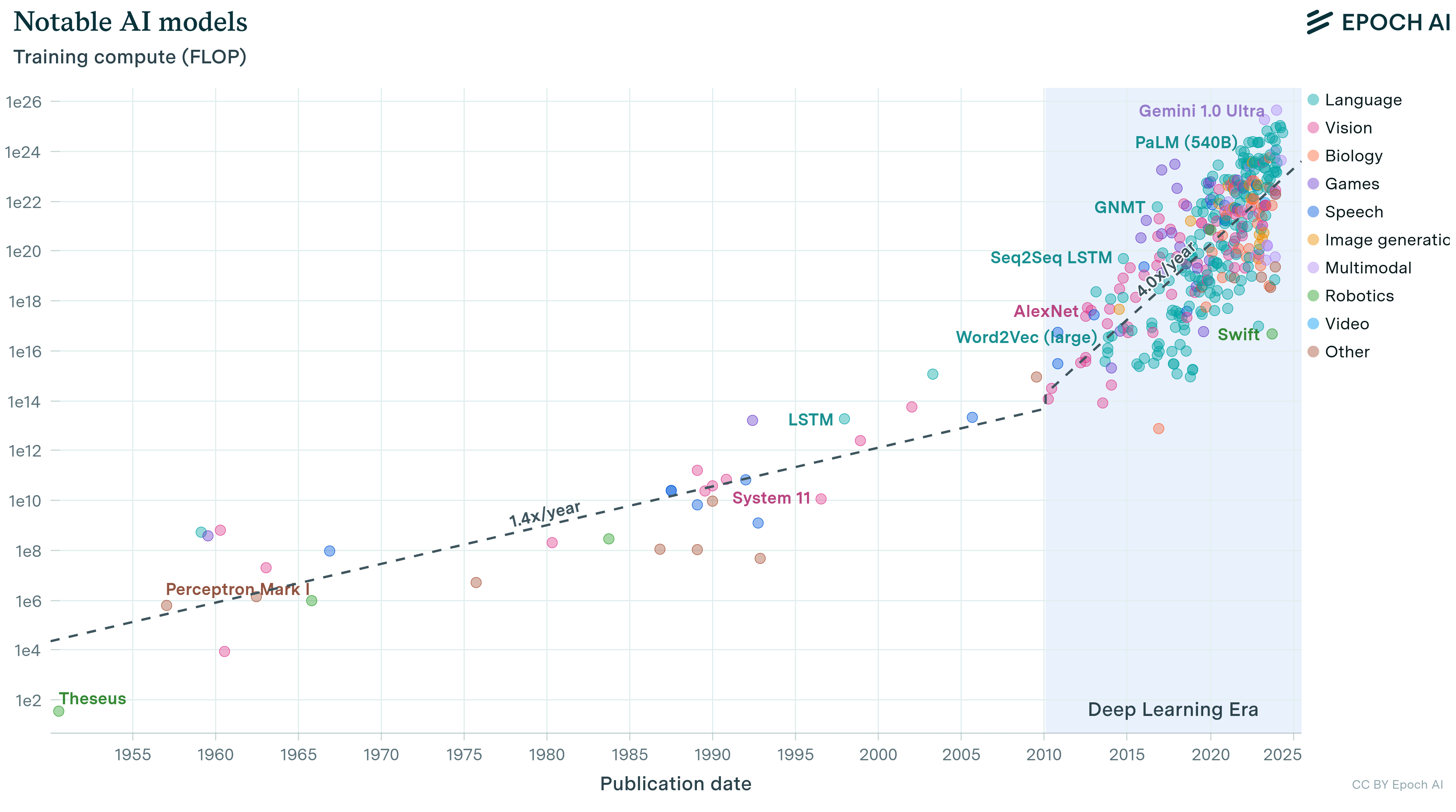](https://mlsysbook.ai/contents/core/efficient_ai/images/png/compute-trends.png "Figure 2: Model Training Compute Trends: Model training compute is growing at faster and faster rates, especially in the recent deep learning era. Source: [@Sevilla_Heim_Ho_Besiroglu_Hobbhahn_Villalobos_2022.]")
Figure 2: **Model Training Compute Trends**: Model training compute is growing at faster and faster rates, especially in the recent deep learning era. Source: ([Sevilla et al. 2022a](https://mlsysbook.ai/contents/core/efficient_ai/efficient_ai.html#ref-Sevilla_Heim_Ho_Besiroglu_Hobbhahn_Villalobos_2022)
.)
Sevilla, Jaime, Lennart Heim, Anson Ho, Tamay Besiroglu, Marius Hobbhahn, and Pablo Villalobos. 2022a. “Compute Trends Across Three Eras of Machine Learning.” In _2022 International Joint Conference on Neural Networks (IJCNN)_, 1–8. IEEE. [https://doi.org/10.1109/ijcnn55064.2022.9891914](https://doi.org/10.1109/ijcnn55064.2022.9891914)
.
Scaling laws provide a quantitative framework for understanding these trade-offs. They reveal that model performance exhibits predictable patterns as resources increase, following power-law relationships where performance improves consistently but with diminishing returns[4](https://mlsysbook.ai/contents/core/efficient_ai/efficient_ai.html#fn4)
. These laws show that optimal resource allocation requires coordinating model size, dataset size, and computational budget rather than scaling any single dimension in isolation.
4 **Diminishing Returns**: Economic principle where each additional input yields progressively smaller output gains. In ML, doubling compute from 1 to 2 hours might improve accuracy by 5%, but doubling from 100 to 200 hours might improve it by only 0.5%.
Refresher: Transformer Computational Characteristics
Recall from **[Chapter 4: DNN Architectures](https://mlsysbook.ai/contents/core/dnn_architectures/dnn_architectures.html#sec-dnn-architectures)
** that transformers process sequences using self-attention mechanisms that compute relationships between all token pairs. This architecture’s computational cost scales quadratically with sequence length, making resource allocation particularly critical for language models. The term “FLOPs” (floating-point operations) quantifies total computational work, while “tokens” represent the individual text units (typically subwords) that models process during training.
### Compute-Optimal Resource Allocation
Empirical studies of large language models (LLMs) reveal a key insight: for any fixed computational budget, there exists an optimal balance between model size and dataset size (measured in tokens[5](https://mlsysbook.ai/contents/core/efficient_ai/efficient_ai.html#fn5)
) that minimizes training loss.
5 **Tokens**: Individual units of text that language models process, created by breaking text into subword pieces using algorithms like Byte-Pair Encoding (BPE). GPT-3 trained on 300 billion tokens while PaLM used 780 billion tokens, requiring text corpora equivalent to millions of books from web crawls and digitized literature.
6 **FLOPs**: Floating-Point Operations, measuring computational work performed. Modern deep learning models require 10²²-10²⁴ FLOPs for training: GPT-3 used ~3.14 × 10²³ FLOPs (314 sextillion operations), equivalent to running a high-end gaming PC continuously for over 350 years.
7 **Transformer**: Neural network architecture introduced by Vaswani et al. ([Chen et al. 2018](https://mlsysbook.ai/contents/core/efficient_ai/efficient_ai.html#ref-vaswani2017attention)
) that revolutionized NLP through self-attention mechanisms. Unlike sequential RNNs, transformers enable parallel processing during training, forming the foundation of modern large language models including GPT, BERT, T5, and their derivatives.
Chen, Mia Xu, Orhan Firat, Ankur Bapna, Melvin Johnson, Wolfgang Macherey, George Foster, Llion Jones, et al. 2018. “The Best of Both Worlds: Combining Recent Advances in Neural Machine Translation.” In _Proceedings of the 56th Annual Meeting of the Association for Computational Linguistics (Volume 1: Long Papers)_, 5998–6008. Association for Computational Linguistics. [https://doi.org/10.18653/v1/p18-1008](https://doi.org/10.18653/v1/p18-1008)
.
8 **Autoregressive Models**: Language models that generate text by predicting each token based on all preceding tokens in the sequence. GPT-family models exemplify this approach, generating text left-to-right with causal attention masks to ensure each position only attends to previous positions.
[Figure 3](https://mlsysbook.ai/contents/core/efficient_ai/efficient_ai.html#fig-compute-optimal)
illustrates this principle through three related views. The left panel shows ‘IsoFLOP curves,’ where each curve corresponds to a constant number of floating-point operations (FLOPs[6](https://mlsysbook.ai/contents/core/efficient_ai/efficient_ai.html#fn6)
) during transformer[7](https://mlsysbook.ai/contents/core/efficient_ai/efficient_ai.html#fn7)
training. The valleys in these curves identify the most efficient model size for each computational budget when training autoregressive[8](https://mlsysbook.ai/contents/core/efficient_ai/efficient_ai.html#fn8)
language models. The center and right panels reveal how the optimal number of parameters and tokens scales predictably as computational budgets increase, demonstrating the necessity for coordinated scaling to maximize resource utilization.
[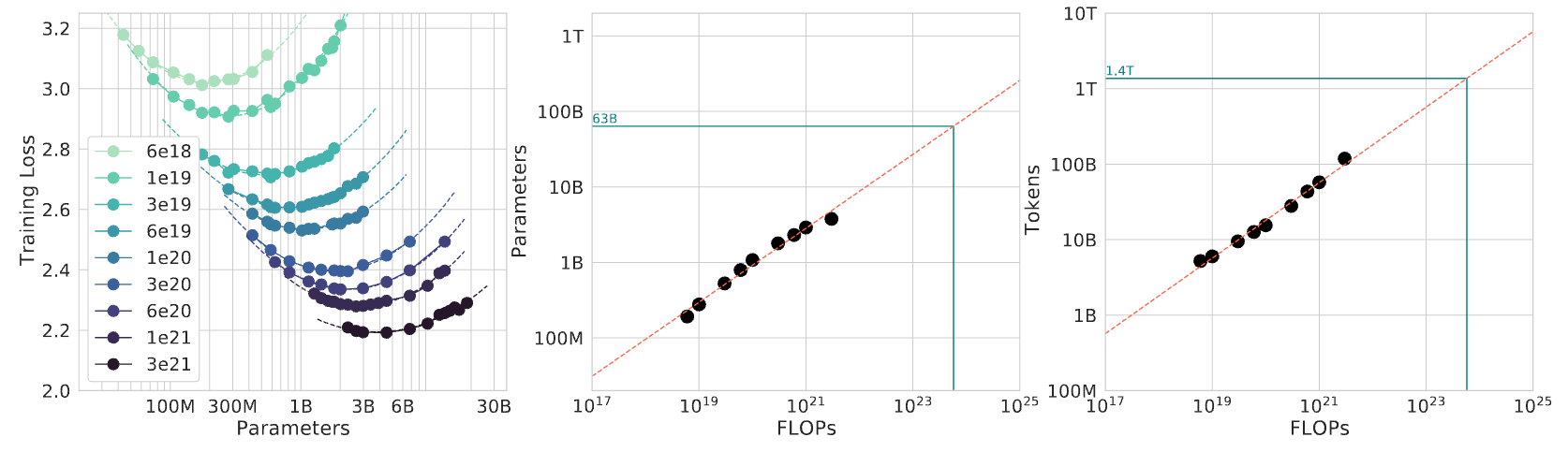](https://mlsysbook.ai/contents/core/efficient_ai/images/png/compute_optimal.png "Figure 3: Optimal Compute Allocation: For fixed computational budgets, language model performance depends on balancing model size and training data volume; the left panel maps training loss across parameter counts, identifying an efficiency sweet spot for each FLOP level. The center and right panels quantify how optimal parameter counts and token requirements scale predictably with increasing compute, demonstrating the need for coordinated scaling of both model and data to maximize resource utilization in large language models. Source: [@hoffmann2022training].")
Figure 3: **Optimal Compute Allocation**: For fixed computational budgets, language model performance depends on balancing model size and training data volume; the left panel maps training loss across parameter counts, identifying an efficiency sweet spot for each FLOP level. The center and right panels quantify how optimal parameter counts and token requirements scale predictably with increasing compute, demonstrating the need for coordinated scaling of both model and data to maximize resource utilization in large language models. Source: ([Hoffmann et al. 2022](https://mlsysbook.ai/contents/core/efficient_ai/efficient_ai.html#ref-hoffmann2022training)
).
Kaplan et al. ([2020](https://mlsysbook.ai/contents/core/efficient_ai/efficient_ai.html#ref-kaplan2020scaling)
) demonstrated that transformer-based language models scale predictably with three factors: the number of model parameters, the volume of the training dataset (measured in tokens), and the total computational budget (measured in floating-point operations). When these factors are augmented proportionally, models exhibit consistent performance improvements without requiring architectural modifications or task-specific tuning.
The practical manifestation of these patterns appears clearly in [Figure 4](https://mlsysbook.ai/contents/core/efficient_ai/efficient_ai.html#fig-kaplan-scaling)
, which presents test loss curves for models spanning from \\(10^3\\) to \\(10^9\\) parameters. The figure reveals two key insights. First, larger models demonstrate superior sample efficiency, achieving target performance levels with fewer training tokens. Second, as computational resources increase, the optimal model size correspondingly grows, with loss decreasing predictably when compute is allocated efficiently.
[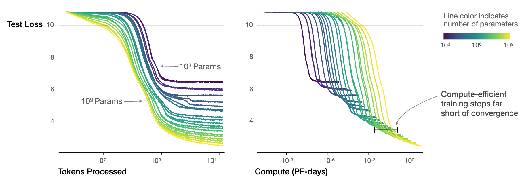](https://mlsysbook.ai/contents/core/efficient_ai/images/png/kaplan_scaling_data_compute.png "Figure 4: Scaling Laws & Compute Optimality: Larger models consistently achieve better performance with increased training data and compute, but diminishing returns necessitate careful resource allocation during training. Optimal model size and training duration depend on the available compute budget, as evidenced by the convergence of loss curves at different parameter scales and training token counts. Source: [@kaplan2020scaling].")
Figure 4: **Scaling Laws & Compute Optimality**: Larger models consistently achieve better performance with increased training data and compute, but diminishing returns necessitate careful resource allocation during training. Optimal model size and training duration depend on the available compute budget, as evidenced by the convergence of loss curves at different parameter scales and training token counts. Source: ([Kaplan et al. 2020](https://mlsysbook.ai/contents/core/efficient_ai/efficient_ai.html#ref-kaplan2020scaling)
).
Kaplan, Jared, Sam McCandlish, Tom Henighan, Tom B. Brown, Benjamin Chess, Rewon Child, Scott Gray, Alec Radford, Jeffrey Wu, and Dario Amodei. 2020. “Scaling Laws for Neural Language Models.” _arXiv Preprint arXiv:2001.08361_, January. [http://arxiv.org/abs/2001.08361v1](http://arxiv.org/abs/2001.08361v1)
.
This theoretical scaling relationship defines optimal compute allocation: for a fixed budget, the relationship \\(D \\propto N^{0.74}\\) ([Hoffmann et al. 2022](https://mlsysbook.ai/contents/core/efficient_ai/efficient_ai.html#ref-hoffmann2022training)
) shows that dataset size \\(D\\) and model size \\(N\\) must grow in coordinated proportions. This means that as model size increases, the dataset should grow at roughly three-quarters the rate to maintain compute-optimal efficiency.
These theoretical predictions assume perfect compute utilization, which becomes challenging in distributed training scenarios. Real-world implementations face communication overhead that scales unfavorably with system size, creating bandwidth bottlenecks that reduce effective utilization. Beyond 100 nodes, communication overhead can reduce expected performance gains by 20-40% depending on workload and interconnect, transforming predicted improvements into more modest real-world results.
### Mathematical Foundations and Operational Regimes
The predictable patterns observed in scaling behavior can be expressed mathematically using power-law relationships, though understanding the intuition behind these patterns proves more important than precise mathematical formulation for most practitioners.
Formal Mathematical Formulation
For readers interested in the formal mathematical framework, scaling laws can be expressed as power-law relationships. The general formulation is:
\\\[ \\mathcal{L}(N) = A N^{-\\alpha} + B \\\]
where loss \\(\\mathcal{L}\\) decreases as resource quantity \\(N\\) increases, following a power-law decay with rate \\(\\alpha\\), plus a baseline constant \\(B\\). Here, \\(\\mathcal{L}(N)\\) represents the loss achieved with resource quantity \\(N\\), \\(A\\) and \\(B\\) are task-dependent constants, and \\(\\alpha\\) is the scaling exponent that characterizes the rate of performance improvement. A larger value of \\(\\alpha\\) signifies more efficient performance improvements with respect to scaling.
These theoretical predictions find strong empirical support across multiple model configurations. [Figure 5](https://mlsysbook.ai/contents/core/efficient_ai/efficient_ai.html#fig-loss-vs-n-d)
shows that early-stopped test loss varies predictably with both dataset size and model size, and learning curves across configurations can be aligned through appropriate parameterization.
#### Resource-Constrained Scaling Regimes
Applying scaling laws in practice requires recognizing three distinct resource allocation regimes that emerge from trade-offs between compute budget, data availability, and optimal resource allocation. These regimes provide practical guidance for system designers navigating resource constraints.
Compute-limited regimes characterize scenarios where available computational resources restrict scaling potential despite abundant training data. Organizations with limited hardware budgets or strict training time constraints operate within this regime. The optimal strategy involves training smaller models for longer periods, maximizing utilization of available compute through extended training schedules rather than larger architectures. This approach proves particularly relevant for academic institutions, startups, or projects with constrained infrastructure access.
Data-limited regimes emerge when computational resources exceed what can be effectively utilized given dataset constraints. High-resource organizations working with specialized domains, proprietary datasets, or privacy-constrained data often encounter this regime. The optimal strategy involves training larger models for fewer optimization steps, leveraging model capacity to extract maximum information from limited training examples. This regime commonly appears in specialized applications like medical imaging or proprietary commercial datasets.
Optimal regimes (Chinchilla Frontier) represent the balanced allocation of compute and data resources following compute-optimal scaling laws. This regime achieves maximum performance efficiency by scaling model size and training data proportionally, as demonstrated by DeepMind’s Chinchilla model, which outperformed much larger models through optimal resource allocation ([Hoffmann et al. 2022](https://mlsysbook.ai/contents/core/efficient_ai/efficient_ai.html#ref-hoffmann2022training)
). Operating within this regime requires sophisticated resource planning but delivers superior performance per unit of computational investment.
Recognizing these regimes enables practitioners to make informed decisions about resource allocation strategies, avoiding common inefficiencies such as over-parameterized models with insufficient training data or under-parameterized models that fail to utilize available computational resources effectively.
[](https://mlsysbook.ai/contents/core/efficient_ai/de2e4205574ea268bcc1883053f7f000bba4f588.svg "Figure 5: : Loss vs Model and Dataset Size: Early-stopped test loss varies predictably with both dataset size and model size, highlighting the importance of balanced scaling for optimal performance under fixed compute budgets.")
Figure 5: : **Loss vs Model and Dataset Size**: Early-stopped test loss varies predictably with both dataset size and model size, highlighting the importance of balanced scaling for optimal performance under fixed compute budgets.
Scaling laws show that performance improvements follow predictable patterns that change depending on resource availability and exhibit distinct behaviors across different dimensions. Two important types of scaling regimes emerge: **data-driven regimes** that describe how performance changes with dataset size, and **temporal regimes** that describe when in the ML lifecycle we apply additional compute.
#### Data-Limited Scaling Regimes
The relationship between generalization error and dataset size exhibits three distinct regimes, as shown in [Figure 6](https://mlsysbook.ai/contents/core/efficient_ai/efficient_ai.html#fig-data-scaling-regimes)
. When limited examples are available, high generalization error results from inadequate statistical estimates. As data availability increases, generalization error decreases predictably as a function of dataset size, following a power-law relationship that provides the most practical benefit from data scaling. Eventually, performance reaches saturation, approaching a floor determined by inherent data limitations or model capacity, beyond which additional data yields negligible improvements.
[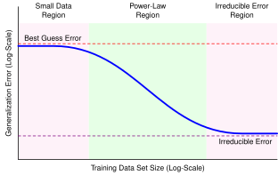](https://mlsysbook.ai/contents/core/efficient_ai/54926858636f497bd98ce136bee5c4785ec5dc9d.svg "Figure 6: : Data Scaling Regimes: The relationship between dataset size and generalization error follows distinct scaling regimes. Increasing dataset size initially reduces generalization error following a power-law relationship, but eventually plateaus at an irreducible error floor determined by inherent data limitations or model capacity [@hestness2017deep]. This behavior exposes diminishing returns from data scaling and informs practical decisions about data collection efforts in machine learning systems.")
Figure 6: : **Data Scaling Regimes**: The relationship between dataset size and generalization error follows distinct scaling regimes. Increasing dataset size initially reduces generalization error following a power-law relationship, but eventually plateaus at an irreducible error floor determined by inherent data limitations or model capacity ([Hestness et al. 2017](https://mlsysbook.ai/contents/core/efficient_ai/efficient_ai.html#ref-hestness2017deep)
). This behavior exposes diminishing returns from data scaling and informs practical decisions about data collection efforts in machine learning systems.
Hestness, Joel, Sharan Narang, Newsha Ardalani, Gregory Diamos, Heewoo Jun, Hassan Kianinejad, Md. Mostofa Ali Patwary, Yang Yang, and Yanqi Zhou. 2017. “Deep Learning Scaling Is Predictable, Empirically.” _arXiv Preprint arXiv:1712.00409_, December. [http://arxiv.org/abs/1712.00409v1](http://arxiv.org/abs/1712.00409v1)
.
This three-regime pattern manifests across different resource dimensions beyond data alone. Operating within the power-law region provides the most reliable return on resource investment. Reaching this regime requires minimum resource thresholds, while maintaining operation within it demands careful allocation to avoid premature saturation.
#### Temporal Scaling Regimes
While data-driven regimes characterize how performance varies with dataset size, a complementary perspective examines temporal allocation of compute resources within the ML lifecycle. Recent research has identified three distinct **temporal scaling regimes** characterizing different stages of model development and deployment.
**Pre-training scaling** encompasses the traditional domain of scaling laws, characterizing how model performance improves with larger architectures, expanded datasets, and increased compute during initial training. Extensive study in foundation models has established clear power-law relationships between resources and capabilities.
**Post-training scaling** characterizes improvements achieved after initial training through techniques including fine-tuning, prompt engineering, and task-specific adaptation. This regime has gained prominence with foundation models, where adaptation rather than retraining frequently provides the most efficient path to enhanced performance under moderate resource requirements.
**Test-time scaling** characterizes how performance improvements result from additional compute allocation during inference without modifying model parameters. This encompasses methods including ensemble prediction, chain-of-thought prompting, and iterative refinement, enabling models to allocate additional processing time per input.
[Figure 7](https://mlsysbook.ai/contents/core/efficient_ai/efficient_ai.html#fig-scaling-regimes)
shows these temporal regimes exhibit distinct characteristics in computational resource allocation for performance improvement. Pre-training demands massive resources while providing broad capabilities, post-training offers targeted enhancements under moderate requirements, and test-time scaling enables flexible performance-compute trade-offs adjustable per inference.
[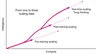](https://mlsysbook.ai/contents/core/efficient_ai/78391c07afda8b90af1af45f04f4817ba07d3d3e.svg "Figure 7: : Temporal Scaling Regimes: Different temporal scaling regimes offer distinct approaches to improving model performance with varying compute investments. Pre-training establishes broad capabilities through large-scale training from scratch, post-training refines existing models through additional training phases, and test-time scaling dynamically allocates compute during inference to enhance per-sample results. Understanding these regimes clarifies the trade-offs between upfront investment and flexible, on-demand resource allocation for optimal system performance.")
Figure 7: : **Temporal Scaling Regimes**: Different temporal scaling regimes offer distinct approaches to improving model performance with varying compute investments. Pre-training establishes broad capabilities through large-scale training from scratch, post-training refines existing models through additional training phases, and test-time scaling dynamically allocates compute during inference to enhance per-sample results. Understanding these regimes clarifies the trade-offs between upfront investment and flexible, on-demand resource allocation for optimal system performance.
Data-driven and temporal scaling regimes are crucial for system design, revealing multiple paths to performance improvement beyond scaling training resources alone. For resource-constrained deployments, post-training and test-time scaling may provide more practical approaches than complete model retraining, while data-efficient techniques enable effective system operation within the power-law regime using smaller datasets.
### Practical Applications in System Design
Scaling laws provide powerful insights for practical system design and resource planning. Consistent observation of power-law trends indicates that within well-defined operational regimes, model performance depends predominantly on scale rather than idiosyncratic architectural innovations. However, diminishing returns phenomena indicate that each additional improvement requires exponentially increased resources while delivering progressively smaller benefits.
OpenAI’s development of GPT-3 demonstrates this principle. Rather than conducting expensive architecture searches, the authors applied scaling laws derived from earlier experiments to determine optimal training dataset size and model parameter count ([Brown et al. 2020](https://mlsysbook.ai/contents/core/efficient_ai/efficient_ai.html#ref-brown2020language)
). They scaled an established transformer architecture along the compute-optimal frontier to 175 billion parameters and approximately 300 billion tokens, enabling advance prediction of model performance and resource requirements. This methodology demonstrated the practical application of scaling laws in large-scale system planning.
Brown, Tom B, Benjamin Mann, Nick Ryder, Melanie Subbiah, Jared Kaplan, Prafulla Dhariwal, Arvind Neelakantan, et al. 2020. “Language Models Are Few-Shot Learners.” _Advances in Neural Information Processing Systems_ 33: 1877–1901.
Scaling laws serve multiple practical functions in system design. They enable practitioners to estimate returns on investment for different resource allocations during resource budgeting. Under fixed computational budgets, designers can utilize empirical scaling curves to determine optimal performance improvement strategies across model size, dataset expansion, or training duration.
System designers can utilize scaling trends to identify when architectural changes yield significant improvements relative to gains achieved through scaling alone, thereby avoiding exhaustive architecture search. When a model family exhibits favorable scaling behavior, scaling the existing architecture may prove more effective than transitioning to more complex but unvalidated designs.
In edge and embedded environments with constrained resource budgets, understanding performance degradation under model scaling enables designers to select smaller configurations delivering acceptable accuracy within deployment constraints. By quantifying scale-performance trade-offs, scaling laws identify when brute-force scaling becomes inefficient and indicate the necessity for alternative approaches including model compression, efficient knowledge transfer, sparsity techniques, and hardware-aware design.
Scaling laws also function as diagnostic instruments. Performance plateaus despite increased resources may indicate dimensional saturation—such as inadequate data relative to model size—or inefficient computational resource utilization. This diagnostic capability renders scaling laws both predictive and prescriptive, facilitating systematic bottleneck identification and resolution.
### Sustainability and Cost Implications
Scaling laws illuminate pathways to performance enhancement while revealing rapidly escalating resource demands. As models expand, training and deployment resource requirements grow disproportionately, creating tension between performance gains through scaling and system efficiency.
Training large-scale models necessitates substantial processing power, typically requiring distributed infrastructures[9](https://mlsysbook.ai/contents/core/efficient_ai/efficient_ai.html#fn9)
comprising hundreds or thousands of accelerators. State-of-the-art language model training may require tens of thousands of GPU-days, consuming millions of kilowatt-hours of electricity. These distributed training systems introduce additional complexity around communication overhead, synchronization, and scaling efficiency, as detailed in **[Chapter 8: AI Training](https://mlsysbook.ai/contents/core/training/training.html#sec-ai-training)
**. Energy demands have outpaced Moore’s Law improvements, raising critical questions about long-term sustainability.
9 **Distributed Infrastructure**: Computing systems that spread ML workloads across multiple machines connected by high-speed networks. OpenAI’s GPT-4 training likely used thousands of NVIDIA A100 GPUs connected via InfiniBand, requiring careful orchestration to avoid communication bottlenecks.
Large models require extensive, high-quality, diverse datasets to achieve their full potential. Data collection, cleansing, and labeling processes consume considerable time and resources. As models approach saturation of available high-quality data, particularly in natural language processing, additional performance gains through data scaling become increasingly difficult to achieve. This reality underscores data efficiency as a necessary complement to brute-force scaling approaches.
The financial and environmental implications compound these challenges. Training runs for large foundation models can incur millions of dollars in computational expenses, and associated carbon footprints[10](https://mlsysbook.ai/contents/core/efficient_ai/efficient_ai.html#fn10)
have garnered increasing scrutiny. These costs limit accessibility to cutting-edge research and exacerbate disparities in access to advanced AI systems. The democratization challenges introduced by efficiency barriers connect directly to accessibility goals addressed in **[Chapter 19: AI for Good](https://mlsysbook.ai/contents/core/ai_for_good/ai_for_good.html#sec-ai-good)
**. Comprehensive approaches to environmental sustainability in ML systems, including carbon footprint measurement and green computing practices, are explored in **[Chapter 18: Sustainable AI](https://mlsysbook.ai/contents/core/sustainable_ai/sustainable_ai.html#sec-sustainable-ai)
**.
10 **Carbon Emissions**: Training GPT-3 generated approximately 502 tons of CO₂ equivalent, comparable to annual emissions of 123 gasoline-powered vehicles. Modern ML practices increasingly incorporate carbon tracking using tools like CodeCarbon and the ML CO2 Impact calculator.
These trade-offs demonstrate that scaling laws provide valuable frameworks for understanding performance growth but do not constitute unencumbered paths to improvement. Each incremental performance gain requires evaluation against corresponding resource requirements. As systems approach practical scaling limits, emphasis must transition from scaling alone to efficient scaling—a comprehensive approach balancing performance, cost, energy consumption, and environmental impact.
### Scaling Law Breakdown Conditions
Scaling laws exhibit remarkable consistency within specific operational regimes but possess inherent limitations. As systems expand, they inevitably encounter boundaries where underlying assumptions of smooth, predictable scaling cease to hold. These breakdown points expose critical inefficiencies and emphasize the necessity for refined system design approaches.
For scaling laws to remain valid, model size, dataset size, and computational budget must be augmented in coordinated fashion. Over-investment in one dimension while maintaining others constant often results in suboptimal outcomes. For example, increasing model size without expanding training datasets may induce overfitting, while increasing computational resources without model redesign may lead to inefficient utilization ([Hoffmann et al. 2022](https://mlsysbook.ai/contents/core/efficient_ai/efficient_ai.html#ref-hoffmann2022training)
).
Hoffmann, Jordan, Sebastian Borgeaud, Arthur Mensch, Elena Buchatskaya, Trevor Cai, Eliza Rutherford, Diego de Las Casas, et al. 2022. “Training Compute-Optimal Large Language Models.” _arXiv Preprint arXiv:2203.15556_, March. [http://arxiv.org/abs/2203.15556v1](http://arxiv.org/abs/2203.15556v1)
.
Large-scale models require carefully tuned training schedules and learning rates to fully utilize available resources. When compute is insufficiently allocated due to premature stopping, batch size misalignment, or ineffective parallelism, models may fail to reach performance potential despite significant infrastructure investment.
Scaling laws presuppose continued performance improvement with sufficient training data. However, in numerous domains, availability of high-quality, human-annotated data is finite. As models consume increasingly large datasets, they reach points of diminishing marginal utility where additional data contributes minimal new information. Beyond this threshold, larger models may exhibit memorization rather than generalization.
As models grow, they demand greater memory bandwidth[11](https://mlsysbook.ai/contents/core/efficient_ai/efficient_ai.html#fn11)
, interconnect capacity, and I/O throughput. These hardware limitations become increasingly challenging even with specialized accelerators. Distributing trillion-parameter models across clusters necessitates meticulous management of data parallelism, communication overhead, and fault tolerance.
11 **Memory Bandwidth**: The rate at which data can be read from or written to memory, measured in GB/s. NVIDIA H100 provides 3.35 TB/s memory bandwidth vs. typical DDR5 RAM’s 51 GB/s, a 65× difference critical for handling large model parameters.
At extreme scales, models may approach limits of what can be learned from training distributions. Performance on benchmarks may continue improving, but these improvements may no longer reflect meaningful gains in generalization or understanding. Models may become increasingly brittle, susceptible to adversarial examples, or prone to generating plausible but inaccurate outputs.
[Table 1](https://mlsysbook.ai/contents/core/efficient_ai/efficient_ai.html#tbl-scaling-breakdown)
synthesizes the primary causes of scaling failure, outlining typical breakdown types, underlying causes, and representative scenarios as a reference for anticipating inefficiencies and guiding balanced system design.
Table 1: **Scaling Breakdown Types**: Unbalanced scaling across model size, data volume, and compute resources leads to specific failure modes, such as overfitting or diminishing returns, impacting system performance and efficiency. The table categorizes these breakdowns, identifies their root causes, and provides representative scenarios to guide more effective system design and resource allocation.
| | | | |
| --- | --- | --- | --- |
| **Model Size** | Overfitting | Model capacity exceeds available data | Billion-parameter model on limited dataset |
| **Data Volume** | Diminishing Returns | Saturation of new or diverse information | Scaling web text beyond useful threshold |
| **Compute Budget** | Underutilized Resources | Insufficient training steps or inefficient use | Large model with truncated training duration |
| **Imbalanced Scaling** | Inefficiency | Uncoordinated increase in model/data/compute | Doubling model size without more data or time |
| **All Dimensions** | Semantic Saturation | Exhaustion of learnable patterns in the domain | No further gains despite scaling all inputs |
These breakdown points demonstrate that scaling laws describe empirical regularities under specific conditions that become increasingly difficult to maintain at scale. As machine learning systems continue evolving, discerning where and why scaling ceases to be effective becomes necessary, driving development of strategies that enhance performance without relying solely on scale.
### Integrating Efficiency with Scaling
The limitations exposed by scaling laws (data saturation, infrastructure bottlenecks, and diminishing returns) demonstrate that brute-force scaling alone cannot deliver sustainable AI systems. These constraints necessitate a shift from expanding scale to achieving greater efficiency with reduced resources.
This transition requires coordinated optimization across three interconnected dimensions: **algorithmic efficiency** addresses computational intensity through better model design, **compute efficiency** maximizes hardware utilization to translate algorithmic improvements into practical gains, and **data efficiency** extracts maximum information from limited examples as high-quality data becomes scarce. Together, these dimensions provide systematic approaches to achieving performance goals that scaling alone cannot sustainably deliver, while addressing broader concerns about equitable access to AI capabilities and environmental impact.
Having examined how scaling laws reveal fundamental constraints, we now turn to the efficiency framework that provides concrete strategies for operating effectively within these constraints. The following section details how the three efficiency dimensions work together to enable sustainable, accessible machine learning systems.
**Self-Check: Question 1.3**
1. What is a key insight from scaling laws in machine learning?
1. Model performance improves linearly with increased computational resources.
2. Larger models always require less training data to achieve state-of-the-art performance.
3. Performance improvements follow predictable power-law relationships with model size, dataset size, and compute budget.
4. Scaling laws suggest that model architecture is the primary driver of performance improvements.
2. Explain the trade-offs involved in scaling machine learning models in terms of computational resources and performance.
3. Order the following models by their parameter size: (1) GPT-1, (2) GPT-2, (3) GPT-3.
4. True or False: According to scaling laws, increasing model size without increasing dataset size can lead to overfitting.
[See Answers →](https://mlsysbook.ai/contents/core/efficient_ai/efficient_ai.html#quiz-answer-sec-efficient-ai-ai-scaling-laws-a043)
The Efficiency Framework
------------------------
The constraint identified through scaling laws (that continued progress requires systematic efficiency optimization) motivates three complementary efficiency dimensions. Each dimension addresses a specific limitation: algorithmic efficiency tackles computational intensity, compute efficiency addresses hardware utilization gaps, and data efficiency solves the data saturation problem.
Together, these three dimensions provide a systematic framework for addressing the constraints that scaling laws reveal. Targeted optimizations across algorithmic design, hardware utilization, and data usage can achieve what brute-force scaling cannot: sustainable, accessible, high-performance AI systems.
### Multi-Dimensional Efficiency Synergies
Optimal performance requires coordinated optimization across multiple dimensions. No single resource—whether model parameters, training data, or compute budget—can be scaled indefinitely to achieve efficiency. Modern techniques demonstrate the potential: 10-100x gains in algorithmic efficiency through optimized architectures, 5-50x improvements in hardware utilization through specialized processors, and 10-1000x reductions in data requirements through advanced learning methods.
The power of this framework emerges from interconnections between dimensions, as depicted in [Figure 8](https://mlsysbook.ai/contents/core/efficient_ai/efficient_ai.html#fig-evolution-efficiency)
. Algorithmic innovations often enable better hardware utilization, while hardware advances unlock new algorithmic possibilities. Data-efficient techniques reduce computational requirements, while compute-efficient methods enable training on larger datasets. Understanding these synergies is essential for building practical ML systems.
[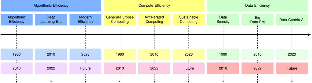](https://mlsysbook.ai/contents/core/efficient_ai/2abdd66045808c7d07317e46f41d4af3ac1aea8a.svg "Figure 8: : Historical Efficiency Trends: Algorithmic, computational, and data efficiency have each contributed to substantial gains in AI capabilities, though at different rates and with diminishing returns. Understanding these historical trends clarifies the interplay between these efficiency dimensions and informs strategies for scaling machine learning systems in data-limited environments.")
Figure 8: : **Historical Efficiency Trends**: Algorithmic, computational, and data efficiency have each contributed to substantial gains in AI capabilities, though at different rates and with diminishing returns. Understanding these historical trends clarifies the interplay between these efficiency dimensions and informs strategies for scaling machine learning systems in data-limited environments.
The specific priorities vary across deployment environments. Cloud systems with abundant resources prioritize scalability and throughput, while edge devices face severe memory and power constraints. Mobile applications must balance performance with battery life, and TinyML deployments demand extreme resource efficiency. Understanding these context-specific patterns enables designers to make informed decisions about which efficiency dimensions to prioritize and how to address inevitable trade-offs between them.
### Achieving Algorithmic Efficiency
Algorithmic efficiency achieves maximum performance per unit of computation through optimized model architectures and training procedures. Modern techniques achieve 10-100x improvements in computational requirements while maintaining or improving accuracy, providing the most direct path to practical AI deployment.
The foundation for these improvements lies in a key observation: most neural networks are dramatically overparameterized. The lottery ticket hypothesis reveals that networks contain sparse subnetworks, typically 10-20% of original parameters (though this varies significantly by architecture and task), that achieve comparable accuracy when trained in isolation ([Frankle and Carbin 2019](https://mlsysbook.ai/contents/core/efficient_ai/efficient_ai.html#ref-frankle2019lottery)
). This discovery transforms compression into a principled approach: large models serve as initialization strategies for finding efficient architectures.
Frankle, Jonathan, and Michael Carbin. 2019. “The Lottery Ticket Hypothesis: Finding Sparse, Trainable Neural Networks.” In _International Conference on Learning Representations_. [https://openreview.net/forum?id=rJl-b3RcF7](https://openreview.net/forum?id=rJl-b3RcF7)
.
#### Model Compression Fundamentals
Three major approaches dominate modern algorithmic efficiency, each targeting different aspects of model inefficiency:
**Model Compression** systematically removes redundant components from neural networks. Pruning techniques achieve 2-4x inference speedup with 1-3% accuracy loss by removing unnecessary weights and structures. Research demonstrates that ResNet-50 can be reduced to 20% of original parameters while maintaining 99% of ImageNet accuracy ([Gholami et al. 2021](https://mlsysbook.ai/contents/core/efficient_ai/efficient_ai.html#ref-gholami2021survey)
). The specific pruning algorithms—including magnitude-based selection, structured vs. unstructured approaches, and layer-wise sensitivity analysis—are covered in detail in **[Chapter 10: Model Optimizations](https://mlsysbook.ai/contents/core/optimizations/optimizations.html#sec-model-optimizations)
**.
Gholami, Amir, Sehoon Kim, Zhen Dong, Zhewei Yao, Michael W. Mahoney, and Kurt Keutzer. 2021. “A Survey of Quantization Methods for Efficient Neural Network Inference.” _arXiv Preprint arXiv:2103.13630_, March. [http://arxiv.org/abs/2103.13630v3](http://arxiv.org/abs/2103.13630v3)
.
Jacob, Benoit, Skirmantas Kligys, Bo Chen, Menglong Zhu, Matthew Tang, Andrew Howard, Hartwig Adam, and Dmitry Kalenichenko. 2018. “Quantization and Training of Neural Networks for Efficient Integer-Arithmetic-Only Inference.” In _2018 IEEE/CVF Conference on Computer Vision and Pattern Recognition_, 2704–13. IEEE. [https://doi.org/10.1109/cvpr.2018.00286](https://doi.org/10.1109/cvpr.2018.00286)
.
**Precision Optimization** reduces computational requirements through quantization, which maps high-precision floating-point values to lower-precision representations. Neural networks demonstrate inherent robustness to precision reduction, with INT8 quantization achieving 4x memory reduction and 2-4x inference speedup while typically maintaining 98-99% of FP32 accuracy ([Jacob et al. 2018](https://mlsysbook.ai/contents/core/efficient_ai/efficient_ai.html#ref-Jacob_et_al_2018)
). Modern techniques range from simple post-training quantization to sophisticated quantization-aware training. The specific quantization algorithms, calibration methods, and training procedures are detailed in **[Chapter 10: Model Optimizations](https://mlsysbook.ai/contents/core/optimizations/optimizations.html#sec-model-optimizations)
**.
**Knowledge Transfer** distills capabilities from large teacher models into efficient student models. Knowledge distillation[12](https://mlsysbook.ai/contents/core/efficient_ai/efficient_ai.html#fn12)
achieves 40-60% parameter reduction while retaining 95-97% of original performance, addressing both computational efficiency and data efficiency by requiring fewer training examples. The specific distillation algorithms, loss functions, and training procedures are covered in **[Chapter 10: Model Optimizations](https://mlsysbook.ai/contents/core/optimizations/optimizations.html#sec-model-optimizations)
**.
12 **Knowledge Distillation**: Technique where a large “teacher” model transfers knowledge to a smaller “student” model by training the student to mimic the teacher’s output probabilities. DistilBERT achieves ~97% of BERT’s performance on GLUE benchmark with 40% fewer parameters and 60% faster inference through distillation.
#### Hardware-Algorithm Co-Design
Algorithmic optimizations alone are insufficient; their practical benefits depend on hardware-software co-design. Optimization techniques must be tailored to target hardware characteristics (memory bandwidth, compute capabilities, and precision support) to achieve real-world speedups. For example, INT8 quantization achieves 2.3x speedup on NVIDIA V100 GPUs with tensor core support but may provide minimal benefit on hardware lacking specialized integer instructions.
Successful co-design requires understanding whether workloads are memory-bound (limited by data movement) or compute-bound (limited by processing capacity), then applying optimizations that address the actual bottleneck. Techniques like operator fusion reduce memory traffic by combining operations, while precision reduction exploits specialized hardware units. While **[Chapter 10: Model Optimizations](https://mlsysbook.ai/contents/core/optimizations/optimizations.html#sec-model-optimizations)
** covers the algorithmic aspects of hardware-aware optimization, **[Chapter 11: AI Acceleration](https://mlsysbook.ai/contents/core/hw_acceleration/hw_acceleration.html#sec-ai-acceleration)
** details how systematic co-design approaches leverage specific hardware architectures for maximum efficiency.
#### Architectural Innovation for Efficiency
Modern efficiency requires architectures designed for resource constraints. Models like MobileNet[13](https://mlsysbook.ai/contents/core/efficient_ai/efficient_ai.html#fn13)
, EfficientNet[14](https://mlsysbook.ai/contents/core/efficient_ai/efficient_ai.html#fn14)
, and SqueezeNet[15](https://mlsysbook.ai/contents/core/efficient_ai/efficient_ai.html#fn15)
demonstrate that compact designs can deliver high performance through architectural innovations rather than scaling up existing designs.
13 **MobileNet**: Efficient neural network architecture using depthwise separable convolutions, achieving ~50× fewer parameters than traditional models. MobileNet-v1 has only 4.2M parameters vs. VGG-16’s ~138M, enabling deployment on smartphones with <100MB memory.
14 **EfficientNet**: Architecture achieving state-of-the-art accuracy with superior parameter efficiency. EfficientNet-B7 achieves 84.3% ImageNet top-1 accuracy (84.4% in some reports) with 66M parameters, compared to ResNet-152’s 77.0% accuracy with approximately 60M parameters.
15 **SqueezeNet**: Compact CNN architecture achieving AlexNet-level accuracy with 50× fewer parameters (1.25M vs. 60M). Demonstrated that clever architecture design can dramatically reduce model size without sacrificing performance.
Different deployment contexts require different efficiency trade-offs. Cloud inference prioritizes throughput and can tolerate higher memory usage, favoring parallel-friendly operations. Edge deployment prioritizes latency and memory efficiency, requiring architectures that minimize memory access. Mobile deployment constrains energy usage, demanding architectures optimized for energy-efficient operations.
#### Parameter-Efficient Adaptation
Parameter-efficient fine-tuning[16](https://mlsysbook.ai/contents/core/efficient_ai/efficient_ai.html#fn16)
techniques demonstrate how the three efficiency dimensions work together. These methods update less than 1% of model parameters while achieving full fine-tuning performance, addressing all three efficiency pillars: algorithmic efficiency through reduced parameter updates, compute efficiency through lower memory requirements and faster training, and data efficiency by leveraging pre-trained representations that require fewer task-specific examples.
16 **Parameter-Efficient Fine-tuning**: Methods like LoRA and Adapters that update <1% of model parameters while achieving full fine-tuning performance. Reduces memory requirements from gigabytes to megabytes for large model adaptation.
The practical impact is transformative: fine-tuning GPT-3 traditionally requires storing gradients for 175 billion parameters, consuming over 700GB of GPU memory. LoRA reduces this to under 10GB by learning low-rank decompositions of weight updates, enabling efficient adaptation on single consumer GPUs while requiring only hundreds of examples rather than thousands for effective adaptation.
As [Figure 9](https://mlsysbook.ai/contents/core/efficient_ai/efficient_ai.html#fig-algo-efficiency)
shows, the computational resources needed to train a neural network to achieve AlexNet[17](https://mlsysbook.ai/contents/core/efficient_ai/efficient_ai.html#fn17)
\-level performance on ImageNet[18](https://mlsysbook.ai/contents/core/efficient_ai/efficient_ai.html#fn18)
classification decreased by approximately \\(44\\times\\) between 2012 and 2019. This improvement, which halved every 16 months, outpaced hardware efficiency gains of Moore’s Law[19](https://mlsysbook.ai/contents/core/efficient_ai/efficient_ai.html#fn19)
, demonstrating the role of algorithmic advancements in driving efficiency ([Hernandez, Brown, et al. 2020](https://mlsysbook.ai/contents/core/efficient_ai/efficient_ai.html#ref-Hernandez_et_al_2020)
).
17 **AlexNet**: Groundbreaking CNN by Krizhevsky, Sutskever, and Hinton (2012) that won ImageNet with 15.3% error rate, nearly halving the previous best of 26.2%. Used 60M parameters, two GPUs, and launched the deep learning revolution.
18 **ImageNet**: Large-scale visual recognition dataset with 14+ million images across 20,000+ categories. The annual ImageNet Large Scale Visual Recognition Challenge (ILSVRC) drove computer vision breakthroughs from 2010-2017.
19 **Moore’s Law**: Intel co-founder Gordon Moore’s 1965 observation that transistor density doubles every ~2 years. Traditional Moore’s Law predicted ~2x transistor density every 18-24 months, though this rate has slowed significantly since ~2015, while AI algorithmic efficiency improved 44x in 7 years (2012-2019).
[](https://mlsysbook.ai/contents/core/efficient_ai/42e5ca2c27671b95ab12272cb46750f6894ba650.svg "Figure 9: : Algorithmic Efficiency Progress: Neural network training compute requirements decreased 44× between 2012 and 2019, outpacing hardware improvements and demonstrating the significant impact of algorithmic advancements on model efficiency. Innovations in model architecture and optimization techniques can drive substantial gains in AI system sustainability via this halving of compute every 16 months. Source: [@Hernandez_et_al_2020].")
Figure 9: : **Algorithmic Efficiency Progress**: Neural network training compute requirements decreased 44× between 2012 and 2019, outpacing hardware improvements and demonstrating the significant impact of algorithmic advancements on model efficiency. Innovations in model architecture and optimization techniques can drive substantial gains in AI system sustainability via this halving of compute every 16 months. Source: ([Hernandez, Brown, et al. 2020](https://mlsysbook.ai/contents/core/efficient_ai/efficient_ai.html#ref-Hernandez_et_al_2020)
).
Hernandez, Danny, Tom B. Brown, et al. 2020. “Measuring the Algorithmic Efficiency of Neural Networks.” _OpenAI Blog_. [https://openai.com/research/ai-and-efficiency](https://openai.com/research/ai-and-efficiency)
.
The evolution of algorithmic efficiency, from basic compression to hardware-aware optimization and parameter-efficient adaptation, demonstrates the centrality of these techniques to machine learning progress. As the field advances, algorithmic efficiency will remain central to designing systems that are high-performing, scalable, and sustainable.
### Compute Efficiency
Compute efficiency focuses on the effective use of hardware and computational resources to train and deploy machine learning models. It encompasses strategies for reducing energy consumption, optimizing processing speed, and leveraging hardware capabilities to achieve scalable and sustainable system performance. While this chapter focuses on efficiency principles and trade-offs, the detailed technical implementation of hardware acceleration—including GPU architectures, TPU design, memory systems, and custom accelerators—is covered in **[Chapter 11: AI Acceleration](https://mlsysbook.ai/contents/core/hw_acceleration/hw_acceleration.html#sec-ai-acceleration)
**.
#### From CPUs to AI Accelerators
Compute efficiency’s evolution reveals why specialized hardware became essential. In the early days of machine learning, Central Processing Units (CPUs) shaped what was possible. CPUs excel at sequential processing and complex decision-making but have limited parallelism, typically 4-16 cores optimized for diverse tasks rather than the repetitive matrix operations that dominate machine learning. Training times for models were measured in days or weeks, as even relatively small datasets pushed hardware boundaries.
This CPU-constrained era ended as deep learning models like AlexNet and ResNet[20](https://mlsysbook.ai/contents/core/efficient_ai/efficient_ai.html#fn20)
demonstrated the potential of neural networks, quickly surpassing traditional CPU capabilities. As shown in [Figure 10](https://mlsysbook.ai/contents/core/efficient_ai/efficient_ai.html#fig-comp_efficiency)
, this marked the beginning of exponential growth in compute usage. OpenAI’s analysis reveals that compute used in AI training increased approximately 300,000 times from 2012 to 2018, doubling approximately every 3.4 months during this period—a rate far exceeding Moore’s Law ([Amodei, Hernandez, et al. 2018](https://mlsysbook.ai/contents/core/efficient_ai/efficient_ai.html#ref-Amodei_et_al_2018)
).
20 **ResNet**: Residual Network architecture by He et al. ([He et al. 2016](https://mlsysbook.ai/contents/core/efficient_ai/efficient_ai.html#ref-he2016deep)
) enabling training of very deep networks (152+ layers) through skip connections. Won ImageNet 2015 with 3.6% error rate, surpassing human-level performance for the first time.
He, Kaiming, Xiangyu Zhang, Shaoqing Ren, and Jian Sun. 2016. “Deep Residual Learning for Image Recognition.” In _2016 IEEE Conference on Computer Vision and Pattern Recognition (CVPR)_, 770–78. IEEE. [https://doi.org/10.1109/cvpr.2016.90](https://doi.org/10.1109/cvpr.2016.90)
.
[](https://mlsysbook.ai/contents/core/efficient_ai/33aa5f6d6d13074068a62908b481e9d47cfefd81.svg "Figure 10: : AI Training Compute Growth: AI training experienced a 300,000-fold increase in computational requirements from 2012 to 2019, exceeding the growth rate predicted by Moore’s Law and driving demand for specialized hardware [@Amodei_et_al_2018]. This exponential growth underscores the increasing complexity of AI models and the need for efficient computing infrastructure to support continued progress.")
Figure 10: : **AI Training Compute Growth**: AI training experienced a 300,000-fold increase in computational requirements from 2012 to 2019, exceeding the growth rate predicted by Moore’s Law and driving demand for specialized hardware ([Amodei, Hernandez, et al. 2018](https://mlsysbook.ai/contents/core/efficient_ai/efficient_ai.html#ref-Amodei_et_al_2018)
). This exponential growth underscores the increasing complexity of AI models and the need for efficient computing infrastructure to support continued progress.
Amodei, Dario, Danny Hernandez, et al. 2018. “AI and Compute.” _OpenAI Blog_. [https://openai.com/research/ai-and-compute](https://openai.com/research/ai-and-compute)
.
This rapid growth was driven by adoption of Graphics Processing Units (GPUs), which offered unparalleled parallel processing capabilities. While CPUs might have 16 cores, modern high-end GPUs like the NVIDIA H100 contain over 16,000 CUDA cores[21](https://mlsysbook.ai/contents/core/efficient_ai/efficient_ai.html#fn21)
. Specialized hardware accelerators such as Google’s Tensor Processing Units (TPUs) further revolutionized compute efficiency by designing chips specifically for machine learning workloads, optimizing for specific data types and operations most common in neural networks.
21 **CUDA Cores**: NVIDIA’s parallel processing units optimized for floating-point operations. Unlike CPU cores (designed for complex sequential tasks), CUDA cores are simpler and work together, enabling a single H100 GPU to perform 16,896 parallel operations simultaneously for massive speedup in matrix computations.
#### Sustainable Computing and Energy Awareness
As systems scale further, compute efficiency has become closely tied to sustainability. Training state-of-the-art large language models requires massive computational resources, leading to increased attention on environmental impact. The projected electricity usage of data centers, shown in [Figure 11](https://mlsysbook.ai/contents/core/efficient_ai/efficient_ai.html#fig-datacenter-energy-usage)
, highlights this concern. Between 2010 and 2030, electricity consumption is expected to rise sharply, particularly under worst-case scenarios where it could exceed 8,000 TWh by 2030 ([Jones 2018](https://mlsysbook.ai/contents/core/efficient_ai/efficient_ai.html#ref-jones2018much)
).
[](https://mlsysbook.ai/contents/core/efficient_ai/4c48abde203d26b69977df82d4ef3b8663e9e9d2.svg "Figure 11: : Data Center Energy Projections: Between 2010 and 2030, data center electricity usage is projected to increase sharply, particularly under worst-case scenarios where consumption could exceed 8,000 TWh by 2030 [@jones2018much]. This projection underscores the critical need for improved energy efficiency in AI systems.")
Figure 11: : **Data Center Energy Projections**: Between 2010 and 2030, data center electricity usage is projected to increase sharply, particularly under worst-case scenarios where consumption could exceed 8,000 TWh by 2030 ([Jones 2018](https://mlsysbook.ai/contents/core/efficient_ai/efficient_ai.html#ref-jones2018much)
). This projection underscores the critical need for improved energy efficiency in AI systems.
Jones, Nicola. 2018. “How to Stop Data Centres from Gobbling up the World’s Electricity.” _Nature_ 561 (7722): 163–66. [https://doi.org/10.1038/d41586-018-06610-y](https://doi.org/10.1038/d41586-018-06610-y)
.
This dramatic growth underscores urgency for compute efficiency, as even large data centers face energy constraints due to limitations in electrical grid capacity. Efficiency improvements alone may not guarantee environmental benefits due to a phenomenon known as Jevons Paradox.
Consider the invention of the fuel-efficient car. While each car uses less gas per mile, the lower cost of driving encourages people to drive more often and live further from work. The result can be an _increase_ in total gasoline consumption. This is Jevons Paradox: efficiency gains can be offset by increased consumption. In AI, this means making models 10x more efficient might lead to a 100x increase in their use, resulting in a net negative environmental impact if not managed carefully.
Addressing these challenges requires optimizing hardware utilization and minimizing energy consumption in both cloud and edge contexts while being mindful of potential rebound effects from increased deployment.
Key trends include adoption of energy-aware scheduling and resource allocation techniques that distribute workloads efficiently across available hardware ([Patterson et al. 2021](https://mlsysbook.ai/contents/core/efficient_ai/efficient_ai.html#ref-Patterson_et_al_2021)
). Researchers are also developing methods to dynamically adjust precision levels during training and inference, using lower precision operations (e.g., mixed-precision training) to reduce power consumption without sacrificing accuracy.
Patterson, David, Joseph Gonzalez, Quoc Le, Chen Liang, Lluis-Miquel Munguia, Daniel Rothchild, David So, Maud Texier, and Jeff Dean. 2021. “Carbon Emissions and Large Neural Network Training.” _arXiv Preprint arXiv:2104.10350_, April. [http://arxiv.org/abs/2104.10350v3](http://arxiv.org/abs/2104.10350v3)
.
22 **Model Parallelism**: Distributing model components across multiple processors due to memory constraints. GPT-3 (175B parameters) requires 350GB memory, exceeding A100’s 40GB capacity by 9×, necessitating tensor parallelism where each transformer layer splits across 8-16 GPUs with all-gather communication for activation synchronization.
23 **Data Parallelism**: Training method where the same model runs on multiple processors with different data batches. GPT-3 training used data parallelism across thousands of GPUs, processing multiple text sequences simultaneously.
Distributed systems achieve compute efficiency by splitting workloads across multiple machines. Techniques such as model parallelism[22](https://mlsysbook.ai/contents/core/efficient_ai/efficient_ai.html#fn22)
and data parallelism[23](https://mlsysbook.ai/contents/core/efficient_ai/efficient_ai.html#fn23)
allow large-scale models to be trained more efficiently, leveraging clusters of GPUs or TPUs to maximize throughput while minimizing idle time.
At the edge, compute efficiency addresses growing demand for real-time processing in energy-constrained environments. Innovations such as hardware-aware model optimization, lightweight inference engines, and adaptive computing architectures enable highly efficient edge systems critical for applications like autonomous vehicles and smart home devices.
#### Production Deployment Patterns
Real-world efficiency optimization demonstrates practical impact across deployment contexts. Production systems routinely achieve 5-10x efficiency gains through coordinated application of optimization techniques while maintaining 95%+ of original model performance.
Mobile applications achieve 4-7x model size reduction and 3-5x latency improvements through combined quantization, pruning, and distillation, enabling real-time inference on mid-range devices. Modern mobile AI systems distribute workloads across specialized processors (NPU for ultra-low power inference, GPU for parallel compute, CPU for control logic) based on power, performance, and real-time constraints.
Autonomous vehicle systems optimize for safety-critical <10ms latency requirements through hardware-aware architectural design and mixed-precision quantization, processing multiple high-bandwidth sensor streams within strict power and thermal constraints.
Cloud serving infrastructure reduces costs by 70-80% through systematic optimization combining dynamic batching, quantization, and knowledge distillation, serving 4-5x more requests at comparable quality levels.
Edge IoT deployments achieve month-long battery life through extreme model compression and duty-cycle optimization, operating on milliwatt power budgets while maintaining acceptable accuracy for practical applications.
These efficiency gains emerge from systematic optimization strategies that coordinate multiple techniques rather than applying individual optimizations in isolation. The specific optimization sequences, technique combinations, and engineering practices that enable these production results are detailed in **[Chapter 10: Model Optimizations](https://mlsysbook.ai/contents/core/optimizations/optimizations.html#sec-model-optimizations)
**.
Compute efficiency complements algorithmic and data efficiency. Compact models reduce computational requirements, while efficient data pipelines streamline hardware usage. The evolution of compute efficiency (from early reliance on CPUs through specialized accelerators to sustainable computing practices) remains central to building scalable, accessible, and environmentally responsible machine learning systems.
### Data Efficiency
Data efficiency focuses on optimizing the amount and quality of data required to train machine learning models effectively. Data efficiency has emerged as a pivotal dimension, driven by rising costs of data collection, storage, and processing, as well as the limits of available high-quality data.
#### Maximizing Learning from Limited Data
In early machine learning, data efficiency was not a primary focus, as datasets were relatively small and manageable. The challenge was often acquiring enough labeled data to train models effectively. Researchers relied on curated datasets such as [UCI’s Machine Learning Repository](https://archive.ics.uci.edu/)
[24](https://mlsysbook.ai/contents/core/efficient_ai/efficient_ai.html#fn24)
, using feature selection and dimensionality reduction techniques like principal component analysis (PCA)[25](https://mlsysbook.ai/contents/core/efficient_ai/efficient_ai.html#fn25)
to extract maximum value from limited data.
24 **UCI Machine Learning Repository**: Established in 1987 by the University of California, Irvine, one of the most widely-used resources for machine learning datasets. Contains over 600 datasets and has been cited in thousands of research papers.
25 **Principal Component Analysis (PCA)**: Dimensionality reduction technique invented by Karl Pearson in 1901, identifies the most important directions of variation in data. Reduces computational complexity while preserving 90%+ of data variance in many applications.
The advent of deep learning in the 2010s transformed data’s role. Models like AlexNet and GPT-3 demonstrated that larger datasets often led to better performance, marking the beginning of the “big data” era. However, this reliance introduced inefficiencies. Data collection became costly and time-consuming, requiring vast amounts of labeled data for supervised learning.
Researchers developed techniques enhancing data efficiency even as datasets grew. Transfer learning[26](https://mlsysbook.ai/contents/core/efficient_ai/efficient_ai.html#fn26)
allowed pre-trained models to be fine-tuned on smaller datasets, reducing task-specific data needs ([Yosinski et al. 2014](https://mlsysbook.ai/contents/core/efficient_ai/efficient_ai.html#ref-yosinski2014transferable)
). Data augmentation[27](https://mlsysbook.ai/contents/core/efficient_ai/efficient_ai.html#fn27)
artificially expanded datasets by creating new variations of existing samples. Active learning[28](https://mlsysbook.ai/contents/core/efficient_ai/efficient_ai.html#fn28)
prioritized labeling only the most informative data points ([Settles 2012a](https://mlsysbook.ai/contents/core/efficient_ai/efficient_ai.html#ref-Settles_2009)
).
26 **Transfer Learning**: Technique where models pre-trained on large datasets are fine-tuned for specific tasks. ImageNet pre-trained models can achieve high accuracy on new vision tasks with <1000 labeled examples vs. millions needed from scratch.
Yosinski, Jason, Jeff Clune, Yoshua Bengio, and Hod Lipson. 2014. “How Transferable Are Features in Deep Neural Networks?” _Advances in Neural Information Processing Systems_ 27.
27 **Data Augmentation**: Artificially expanding datasets through transformations like rotations, crops, or noise. Can improve model performance by 5-15% and reduce overfitting, especially when labeled data is scarce.
28 **Active Learning**: Iteratively selecting the most informative samples for labeling to maximize learning efficiency. Can achieve target performance with 50-90% less labeled data compared to random sampling.
Settles, Burr. 2012a. _Active Learning_. _Computer Sciences Technical Report_. University of Wisconsin–Madison; Springer International Publishing. [https://doi.org/10.1007/978-3-031-01560-1](https://doi.org/10.1007/978-3-031-01560-1)
.
29 **Data-Centric AI**: Paradigm shift from model-centric to data-centric development, popularized by Andrew Ng in 2021. Focuses on systematically improving data quality rather than just model architecture, often yielding greater performance gains.
As systems continue growing in scale, inefficiencies of large datasets have become apparent. Data-centric AI[29](https://mlsysbook.ai/contents/core/efficient_ai/efficient_ai.html#fn29)
has emerged as a key paradigm, emphasizing data quality over quantity. This approach focuses on enhancing preprocessing, removing redundancy, and improving labeling efficiency. Research shows that careful curation and filtering can achieve comparable or superior performance while using only a fraction of original data volume ([Penedo et al. 2024](https://mlsysbook.ai/contents/core/efficient_ai/efficient_ai.html#ref-penedo2024fineweb)
).
Several techniques support this transition. Self-supervised learning[30](https://mlsysbook.ai/contents/core/efficient_ai/efficient_ai.html#fn30)
enables models to learn meaningful representations from unlabeled data, reducing dependency on expensive human-labeled datasets. Active learning strategies selectively identify the most informative examples for labeling, while curriculum learning[31](https://mlsysbook.ai/contents/core/efficient_ai/efficient_ai.html#fn31)
structures training to progress from simple to complex examples, improving learning efficiency.
30 **Self-Supervised Learning**: Training method where models create their own labels from input data structure, like predicting masked words in BERT. Enables learning from billions of unlabeled examples.
31 **Curriculum Learning**: Training strategy where models learn from easy examples before progressing to harder ones, mimicking human education. Can improve convergence speed by 25-50% and final model performance.
32 **Foundation Models**: Large-scale, general-purpose AI models trained on broad data that can be adapted for many tasks. Term coined by Stanford HAI in 2021, includes models like GPT-3, BERT, and DALL-E.
Data efficiency is particularly important in foundation models[32](https://mlsysbook.ai/contents/core/efficient_ai/efficient_ai.html#fn32)
. As these models grow in scale and capability, they approach limits of available high-quality training data, especially for language tasks, as shown in [Figure 12](https://mlsysbook.ai/contents/core/efficient_ai/efficient_ai.html#fig-running-out-of-human-data)
. This scarcity drives innovation in data processing and curation techniques.
[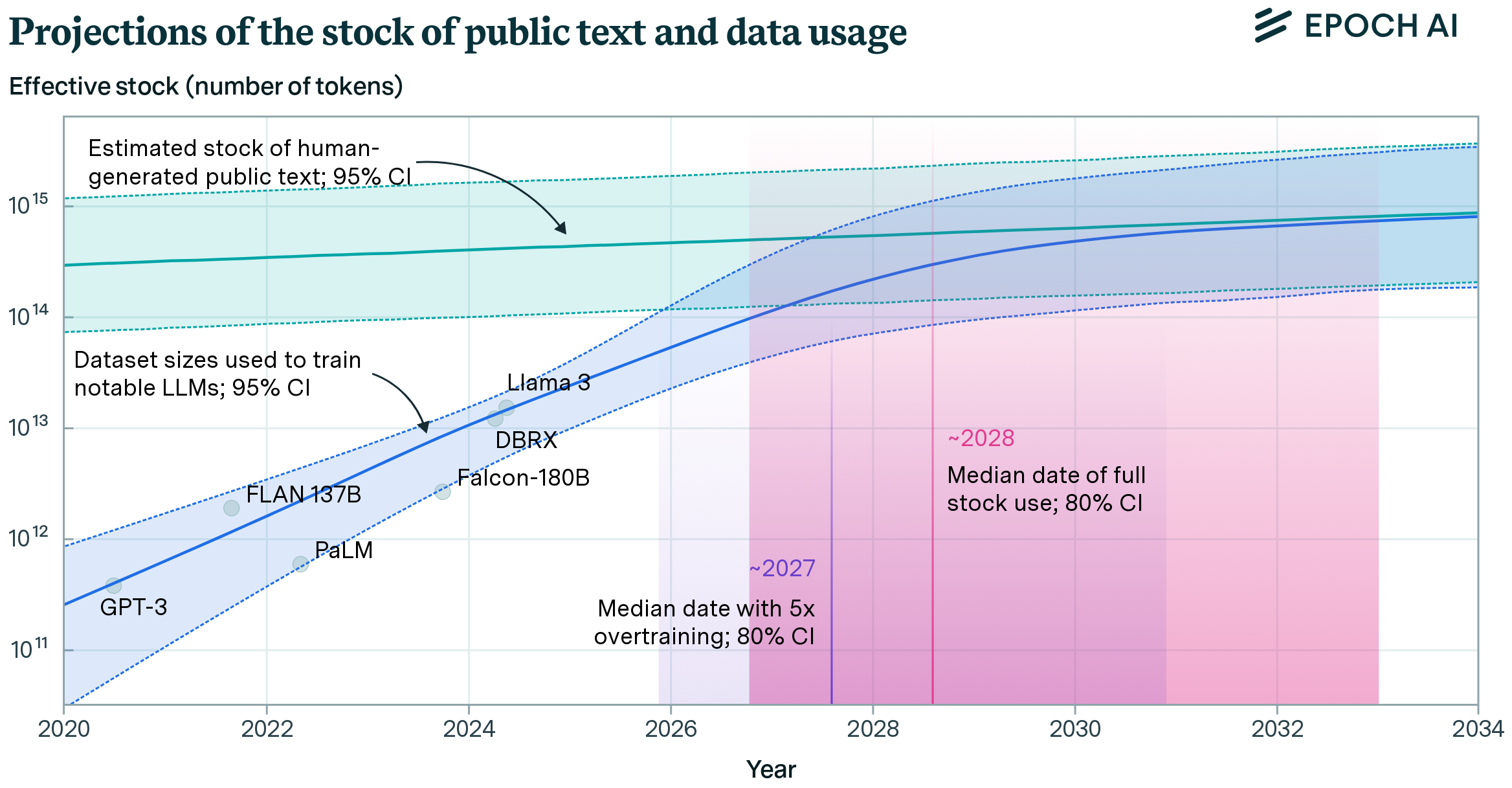](https://mlsysbook.ai/contents/core/efficient_ai/images/png/running_out_of_data.png "Figure 12: Dataset Growth: Foundation models are increasingly trained on vast datasets, reflecting the growing stock of human-generated text. This trend underscores the challenge of data scarcity in maintaining model performance as scale increases. Source: @villalobos_ho_sevilla_besiroglu_heim_hobbhahn_2024.")
Figure 12: **Dataset Growth**: Foundation models are increasingly trained on vast datasets, reflecting the growing stock of human-generated text. This trend underscores the challenge of data scarcity in maintaining model performance as scale increases. Source: Sevilla et al. ([2022b](https://mlsysbook.ai/contents/core/efficient_ai/efficient_ai.html#ref-villalobos_ho_sevilla_besiroglu_heim_hobbhahn_2024)
).
———. 2022b. “Compute Trends Across Three Eras of Machine Learning.” In _2022 International Joint Conference on Neural Networks (IJCNN)_, 1–8. IEEE. [https://doi.org/10.1109/ijcnn55064.2022.9891914](https://doi.org/10.1109/ijcnn55064.2022.9891914)
.
Evidence for data quality’s impact appears across different deployment scales. In Tiny ML[33](https://mlsysbook.ai/contents/core/efficient_ai/efficient_ai.html#fn33)
applications, datasets like Wake Vision demonstrate how performance critically depends on careful data curation ([Banbury et al. 2024](https://mlsysbook.ai/contents/core/efficient_ai/efficient_ai.html#ref-banbury2024wakevisiontailoreddataset)
). At larger scales, research on language models trained on web-scale datasets shows that intelligent filtering and selection strategies significantly improve performance on downstream tasks ([Penedo et al. 2024](https://mlsysbook.ai/contents/core/efficient_ai/efficient_ai.html#ref-penedo2024fineweb)
). **[Chapter 12: Benchmarking AI](https://mlsysbook.ai/contents/core/benchmarking/benchmarking.html#sec-benchmarking-ai)
** establishes rigorous methodologies for measuring these data quality improvements.
33 **TinyML**: Machine learning on microcontrollers and edge devices with <1KB-1MB memory and <1mW power consumption. Enables AI in IoT devices, wearables, and sensors where traditional ML deployment is impossible.
Banbury, Colby, Emil Njor, Andrea Mattia Garavagno, Mark Mazumder, Matthew Stewart, Pete Warden, Manjunath Kudlur, Nat Jeffries, Xenofon Fafoutis, and Vijay Janapa Reddi. 2024. “Wake Vision: A Tailored Dataset and Benchmark Suite for TinyML Computer Vision Applications,” May. [http://arxiv.org/abs/2405.00892v5](http://arxiv.org/abs/2405.00892v5)
.
Penedo, Guilherme, Hynek Kydlı́ček, Loubna Ben allal, Anton Lozhkov, Margaret Mitchell, Colin Raffel, Leandro Von Werra, and Thomas Wolf. 2024. “The FineWeb Datasets: Decanting the Web for the Finest Text Data at Scale.” _arXiv Preprint arXiv:2406.17557_, June. [http://arxiv.org/abs/2406.17557v2](http://arxiv.org/abs/2406.17557v2)
.
This modern era of data efficiency represents a shift in how systems approach data utilization. By focusing on quality over quantity and developing sophisticated techniques for data selection and processing, the field is moving toward more sustainable and effective approaches to model training and deployment. Data efficiency is integral to scalable systems, impacting both model and compute efficiency. Smaller, higher-quality datasets reduce training times and computational demands while enabling better generalization. These principles complement the privacy-preserving techniques explored in **[Chapter 15: Security & Privacy](https://mlsysbook.ai/contents/core/privacy_security/privacy_security.html#sec-security-privacy)
**, where minimizing data requirements enhances both efficiency and user privacy protection.
**Self-Check: Question 1.4**
1. Which of the following best describes the role of algorithmic efficiency in the efficiency framework?
1. Reducing the amount of data needed for training
2. Improving the utilization of hardware resources
3. Maximizing performance per unit of computation
4. Enhancing the scalability of cloud systems
2. Explain how coordinated optimization across algorithmic, compute, and data efficiency can lead to sustainable AI systems.
3. True or False: In mobile applications, data efficiency is prioritized over compute efficiency due to battery life constraints.
4. What is a common trade-off when optimizing for algorithmic efficiency in edge devices?
1. Increased data requirements
2. Reduced model accuracy
3. Higher computational intensity
4. Increased hardware utilization
5. How might you apply the efficiency framework in designing an ML system for autonomous vehicles?
[See Answers →](https://mlsysbook.ai/contents/core/efficient_ai/efficient_ai.html#quiz-answer-sec-efficient-ai-efficiency-framework-c0de)
Real-World Efficiency Strategies
--------------------------------
Having explored each efficiency dimension individually and their interconnections, we examine how these dimensions manifest across different deployment contexts. The efficiency of machine learning systems emerges from understanding relationships between algorithmic, compute, and data efficiency in specific operational environments.
### Context-Specific Efficiency Requirements
The specific priorities and trade-offs vary dramatically across deployment environments. As our opening examples illustrated, these range from cloud systems with abundant resources to edge devices with severe memory and power constraints. [Table 2](https://mlsysbook.ai/contents/core/efficient_ai/efficient_ai.html#tbl-deployment-efficiency-priorities)
maps how these constraints translate into efficiency optimization priorities.
Table 2: **Efficiency Optimization Priorities by Deployment Context**: Each environment demands different trade-offs between algorithmic, compute, and data optimization strategies based on unique constraints. Cloud systems prioritize scalability, edge deployments focus on real-time performance, mobile applications balance performance with battery life, and TinyML demands extreme resource efficiency.
| | | | |
| --- | --- | --- | --- |
| **Cloud** | Cost at scale, energy consumption | Throughput, scalability, operational efficiency | Large language model APIs, recommendation engines, video processing |
| **Edge** | Latency, local compute capacity, connectivity | Real-time performance, power efficiency | Autonomous vehicles, industrial automation, smart cameras |
| **Mobile** | Battery life, memory, thermal limits | Energy efficiency, model size, responsiveness | Voice assistants, photo enhancement, augmented reality |
| **TinyML** | Extreme power/memory constraints | Ultra-low power, minimal model size | IoT sensors, wearables, environmental monitoring |
Understanding these context-specific patterns enables designers to make informed decisions about which efficiency dimensions to prioritize and how to navigate inevitable trade-offs.
### Scalability and Sustainability
System efficiency serves as a driver of environmental sustainability. When systems are optimized for efficiency, they can be deployed at scale while minimizing environmental footprint. This relationship creates a positive feedback loop, as shown in [Figure 13](https://mlsysbook.ai/contents/core/efficient_ai/efficient_ai.html#fig-virtuous-efficiency-cycle)
.
[](https://mlsysbook.ai/contents/core/efficient_ai/8ff5d037eed695d0dcda2db19bf7a200a9084b98.svg "Figure 13: : Efficiency and Sustainability Feedback Loop: Optimized machine learning systems achieve greater scalability, which in turn incentivizes sustainable design practices and further efficiency improvements, creating a reinforcing feedback loop for long-term impact.")
Figure 13: : **Efficiency and Sustainability Feedback Loop**: Optimized machine learning systems achieve greater scalability, which in turn incentivizes sustainable design practices and further efficiency improvements, creating a reinforcing feedback loop for long-term impact.
Efficient systems are inherently scalable. Reducing resource demands through lightweight models, targeted datasets, and optimized compute utilization allows systems to deploy broadly. When efficient systems scale, they amplify their contribution to sustainability by reducing overall energy consumption and computational waste. Sustainability reinforces the need for efficiency, creating a feedback loop that strengthens the entire system.
**Self-Check: Question 1.5**
1. Which deployment context prioritizes real-time performance and power efficiency due to local compute capacity and connectivity constraints?
1. Edge
2. Cloud
3. Mobile
4. TinyML
2. Explain how system efficiency contributes to scalability and sustainability in machine learning deployments.
3. Order the following deployment contexts by their primary efficiency priority from highest to lowest: (1) Cloud, (2) Edge, (3) Mobile, (4) TinyML.
4. True or False: In TinyML deployments, model size is prioritized over power efficiency.
[See Answers →](https://mlsysbook.ai/contents/core/efficient_ai/efficient_ai.html#quiz-answer-sec-efficient-ai-realworld-efficiency-strategies-8387)
Efficiency Trade-offs and Challenges
------------------------------------
The three efficiency dimensions can work synergistically under favorable conditions, but real-world systems often face scenarios where improving one dimension degrades another. The same resource constraints that make efficiency necessary force difficult choices: reducing model size may sacrifice accuracy, optimizing for real-time performance may increase energy consumption, and curating smaller datasets may limit generalization.
### Fundamental Sources of Efficiency Trade-offs
These tensions manifest in various ways across machine learning systems. Understanding their root causes is essential for addressing design challenges. Each efficiency dimension influences the others, creating a dynamic interplay that shapes system performance.
#### Algorithmic Efficiency vs. Compute Requirements
Algorithmic efficiency focuses on designing compact models that minimize computational and memory demands. By reducing model size or complexity, deployment on resource-limited devices becomes feasible. Overly simplifying a model can reduce accuracy, especially for complex tasks. To compensate for this loss, additional computational resources may be required during training or deployment, placing strain on compute efficiency.
#### Compute Efficiency vs. Real-Time Needs
Compute efficiency aims to minimize resources required for training and inference, reducing energy consumption, processing time, and memory use. In scenarios requiring real-time responsiveness (autonomous vehicles, augmented reality), compute efficiency becomes harder to maintain. [Figure 14](https://mlsysbook.ai/contents/core/efficient_ai/efficient_ai.html#fig-efficiency-vs-latency)
illustrates this challenge: real-time systems often require high-performance hardware to process data instantly, conflicting with energy efficiency goals or increasing system costs.
[](https://mlsysbook.ai/contents/core/efficient_ai/1ed2becdb8c20bbfe74e21c91c64885a70a192ca.svg "Figure 14: : Real-Time System Constraints: Autonomous vehicles demand careful balance between computational efficiency and low latency. Increasing processing power to reduce delay can conflict with energy and cost limitations, yet sacrificing latency compromises safety by increasing reaction time and braking distance.")
Figure 14: : **Real-Time System Constraints**: Autonomous vehicles demand careful balance between computational efficiency and low latency. Increasing processing power to reduce delay can conflict with energy and cost limitations, yet sacrificing latency compromises safety by increasing reaction time and braking distance.
#### Data Efficiency vs. Model Generalization
Data efficiency seeks to minimize the amount of data required to train a model without sacrificing performance. By curating smaller, high-quality datasets, training becomes faster and less resource-intensive. Ideally, this reinforces both algorithmic and compute efficiency. However, reducing dataset size can limit diversity, making it harder for models to generalize to unseen scenarios. To address this, additional compute resources or model complexity may be required, creating tension between data efficiency and broader system goals.
### Recurring Trade-off Patterns in Practice
The trade-offs between efficiency dimensions become particularly evident when examining specific scenarios. Complex models with millions or billions of parameters can achieve higher accuracy by capturing intricate patterns, but require significant computational power and memory. A recommendation system in a cloud data center might use a highly complex model for better recommendations, but at the cost of higher energy consumption and operating costs. On resource-constrained devices like smartphones or autonomous vehicles, compact models may operate efficiently but require more sophisticated data preprocessing or training procedures to compensate for reduced capacity.
Energy efficiency and real-time performance often pull systems in opposite directions. Real-time systems like autonomous vehicles or augmented reality applications rely on high-performance hardware to process large volumes of data quickly, but this typically increases energy consumption. An autonomous vehicle must process sensor data from cameras, LiDAR, and radar in real time to make navigation decisions, requiring specialized accelerators that consume significant energy. In edge deployments with battery power or limited energy sources, this trade-off becomes even more critical.
Larger datasets generally provide greater diversity and coverage, enabling models to capture subtle patterns and reduce overfitting risk. However, computational and memory demands of training on large datasets can be substantial. In resource-constrained environments like TinyML deployments, an IoT device monitoring environmental conditions might need a model that generalizes well across varying conditions, but collecting extensive datasets may be impractical due to storage and computational limitations. Smaller, carefully curated datasets or synthetic data may be used to reduce computational strain, but this risks missing key edge cases.
These trade-offs are not merely academic concerns but practical realities that shape system design decisions across all deployment contexts.
**Self-Check: Question 1.6**
1. Which of the following best describes the trade-off between algorithmic efficiency and compute requirements?
1. Reducing model size always improves accuracy.
2. Simplifying models can reduce computational demands but may decrease accuracy.
3. Increasing model complexity always reduces energy consumption.
4. Deploying models on resource-limited devices requires no trade-offs.
2. Explain how real-time performance requirements can conflict with compute efficiency in ML systems.
3. In a production system where energy efficiency is critical, which strategy might be prioritized?
1. Using high-performance GPUs for all tasks.
2. Deploying complex models without considering energy consumption.
3. Ignoring latency requirements to save energy.
4. Optimizing models to run on low-power hardware.
4. In scenarios requiring real-time responsiveness, such as autonomous vehicles, the trade-off between computational efficiency and low latency often requires balancing \_\_\_\_\_\_\_\_ and energy consumption.
5. In your experience with ML systems, how might you address the trade-off between data efficiency and model generalization?
[See Answers →](https://mlsysbook.ai/contents/core/efficient_ai/efficient_ai.html#quiz-answer-sec-efficient-ai-efficiency-tradeoffs-challenges-946d)
Strategic Trade-off Management
------------------------------
The trade-offs inherent in machine learning system design require thoughtful strategies to navigate effectively. Achieving the right balance involves difficult decisions heavily influenced by specific goals and constraints of the deployment environment. Designers can adopt a range of strategies that address unique requirements of different contexts.
### Environment-Driven Efficiency Priorities
Efficiency goals are rarely universal. The specific demands of an application or deployment scenario heavily influence which dimension—algorithmic, compute, or data—takes precedence. Prioritizing the right dimensions based on context is the first step in effectively managing trade-offs.
In Mobile ML deployments, battery life is often the primary constraint, placing a premium on compute efficiency. Energy consumption must be minimized to preserve operational time, so lightweight models are prioritized even if it means sacrificing some accuracy or requiring additional data preprocessing.
In Cloud ML systems, scalability and throughput are paramount. These systems must process large volumes of data and serve millions of users simultaneously. While compute resources are more abundant, energy efficiency and operational costs remain important. Algorithmic efficiency plays a critical role in ensuring systems can scale without overwhelming infrastructure.
Edge ML systems present different priorities. Autonomous vehicles or real-time monitoring systems require low-latency processing for safe and reliable operation, making real-time performance and compute efficiency paramount, often at the expense of energy consumption. However, hardware constraints mean these systems must still carefully manage energy and computational resources.
**TinyML** deployments demand extreme efficiency due to severe hardware and energy limitations. Algorithmic and data efficiency are top priorities, with models highly compact and capable of operating on microcontrollers with minimal memory and compute power, while training relies on small, carefully curated datasets.
### Dynamic Resource Allocation at Inference
System adaptability can be enhanced through dynamic resource allocation during inference. This approach recognizes that resource needs may fluctuate even within specific deployment contexts. By adjusting computational effort at inference time, systems can fine-tune performance to meet immediate demands.
For example, a cloud-based video analysis system might process standard streams with a streamlined model to maintain high throughput, but when a critical event is detected, dynamically allocate more resources to a complex model for higher precision. Similarly, mobile voice assistants might use lightweight models for routine commands to conserve battery, but temporarily activate resource-intensive models for complex queries.
Implementing test-time compute introduces new challenges. Dynamic resource allocation requires sophisticated monitoring and control mechanisms. There are diminishing returns—increasing compute beyond certain thresholds may not yield significant performance improvements. The ability to dynamically increase compute can also create disparities in access to high-performance AI, raising equity concerns. Despite these challenges, test-time compute offers a valuable strategy for enhancing system adaptability.
### End-to-End Co-Design and Automated Optimization
Efficient machine learning systems are rarely the product of isolated optimizations. Achieving balance across efficiency dimensions requires an end-to-end co-design perspective, where each system component is designed in tandem with others. This holistic approach aligns model architectures, hardware platforms, and data pipelines to work seamlessly together.
Co-design becomes essential in resource-constrained environments. Models must align precisely with hardware capabilities—8-bit models require hardware support for efficient integer operations, while pruned models benefit from sparse tensor operations. Edge accelerators often optimize specific operations like convolutions, influencing model architecture choices. Detailed hardware architecture considerations are covered comprehensively in **[Chapter 11: AI Acceleration](https://mlsysbook.ai/contents/core/hw_acceleration/hw_acceleration.html#sec-ai-acceleration)
**.
**Automation and optimization tools** help manage the complexity of navigating trade-offs. Automated machine learning (AutoML)[34](https://mlsysbook.ai/contents/core/efficient_ai/efficient_ai.html#fn34)
enables exploration of different model architectures and hyperparameter configurations. Building on the systematic approach to ML workflows introduced in **[Chapter 5: AI Workflow](https://mlsysbook.ai/contents/core/workflow/workflow.html#sec-ai-workflow)
**, AutoML tools automate many efficiency optimization decisions that traditionally required extensive manual tuning.
34 **AutoML**: Automated machine learning that systematically searches through model architectures, hyperparameters, and data preprocessing options. Google’s AutoML achieved 84.3% ImageNet accuracy vs. human experts’ 78.5%, while reducing development time from months to hours.
35 **Neural Architecture Search (NAS)**: Automated method for discovering optimal neural network architectures. EfficientNet-B7, discovered via NAS, achieved 84.3% ImageNet accuracy with 37M parameters vs. hand-designed ResNeXt-101’s 80.9% with 84M parameters.
Neural architecture search (NAS)[35](https://mlsysbook.ai/contents/core/efficient_ai/efficient_ai.html#fn35)
takes automation further by designing model architectures tailored to specific hardware or deployment scenarios, evaluating a wide range of architectural possibilities to maximize performance while minimizing computational demands.
Data efficiency also benefits from automation. Tools that automate dataset curation, augmentation, and active learning reduce training dataset size without sacrificing performance, prioritizing high-value data points to speed up training and reduce computational overhead ([Settles 2012b](https://mlsysbook.ai/contents/core/efficient_ai/efficient_ai.html#ref-settles2009active)
). **[Chapter 7: AI Frameworks](https://mlsysbook.ai/contents/core/frameworks/frameworks.html#sec-ai-frameworks)
** explores how modern ML frameworks incorporate these automation capabilities.
———. 2012b. _Active Learning_. _University of Wisconsin-Madison Department of Computer Sciences_. Vol. 1648. Springer International Publishing. [https://doi.org/10.1007/978-3-031-01560-1](https://doi.org/10.1007/978-3-031-01560-1)
.
### Measuring and Monitoring Efficiency Trade-offs
Beyond technical automation lies the broader challenge of systematic evaluation. Efficiency optimization necessitates a structured approach assessing trade-offs that extends beyond purely technical considerations. As systems transition from research to production, success criteria must encompass algorithmic performance, economic viability, and operational sustainability.
Costs associated with efficiency improvements manifest across engineering effort (research, experimentation, integration), balanced against ongoing operational expenses of running less efficient systems. Benefits span multiple domains—beyond direct cost reductions, efficient systems often enable qualitatively new capabilities like real-time processing in resource-constrained environments or deployment to edge devices.
This evaluation framework must be complemented by ongoing assessment mechanisms. The dynamic nature of ML systems in production necessitates continuous monitoring of efficiency characteristics. As models evolve, data distributions shift, and infrastructure changes, efficiency properties can degrade. Real-time monitoring enables rapid detection of efficiency regressions, while historical analysis provides insight into longer-term trends, revealing whether efficiency improvements are sustainable under changing conditions.
**Self-Check: Question 1.7**
1. Which of the following is a primary concern in mobile ML deployments?
1. Algorithmic accuracy
2. Scalability
3. Data efficiency
4. Compute efficiency
2. Explain how flexible resource allocation can enhance system adaptability in cloud ML systems.
3. Order the following deployment contexts by their primary efficiency priority from highest to lowest: (1) Mobile ML, (2) Cloud ML, (3) Edge ML, (4) TinyML.
4. In TinyML deployments, the primary focus is on \_\_\_\_ efficiency due to severe hardware and energy limitations.
5. How does co-design contribute to managing trade-offs in resource-constrained ML environments?
[See Answers →](https://mlsysbook.ai/contents/core/efficient_ai/efficient_ai.html#quiz-answer-sec-efficient-ai-strategic-tradeoff-management-0ac8)
Engineering Principles for Efficient AI
---------------------------------------
Designing an efficient machine learning system requires a holistic approach. True efficiency emerges when the entire system is considered as a whole, ensuring trade-offs are balanced across all stages of the ML pipeline from data collection to deployment. This end-to-end perspective transforms system design.
### Holistic Pipeline Optimization
Efficiency is achieved not through isolated optimizations but by considering the entire pipeline as a unified whole. Each stage—data collection, model training, hardware deployment, and inference—contributes to overall system efficiency. Decisions at one stage ripple through the rest, influencing performance, resource use, and scalability.
Data collection and preprocessing are starting points. **[Chapter 6: Data Engineering](https://mlsysbook.ai/contents/core/data_engineering/data_engineering.html#sec-data-engineering)
** provides comprehensive coverage of how data pipeline design decisions cascade through the entire system. Curating smaller, high-quality datasets can reduce computational costs during training while simplifying model design. However, insufficient data diversity may affect generalization, necessitating compensatory measures.
Model training is another critical stage. Architecture choice, optimization techniques, and hyperparameters must consider deployment hardware constraints. A model designed for high-performance cloud systems may emphasize accuracy and scalability, while models for edge devices must balance accuracy with size and energy efficiency.
Deployment and inference demand precise hardware alignment. Each platform offers distinct capabilities—GPUs excel at parallel matrix operations, TPUs optimize specific neural network computations, and microcontrollers provide energy-efficient processing. A smartphone speech recognition system might leverage an NPU’s dedicated convolution units for millisecond-level inference at low power, while an autonomous vehicle’s FPGA processes multiple sensor streams with microsecond-level latency.
An end-to-end perspective ensures trade-offs are addressed holistically rather than shifting inefficiencies between pipeline stages. This systems thinking approach becomes particularly critical when deploying to resource-constrained environments, as explored in **[Chapter 14: On-Device Learning](https://mlsysbook.ai/contents/core/ondevice_learning/ondevice_learning.html#sec-ondevice-learning)
**.
### Lifecycle and Environment Considerations
Efficiency needs differ significantly depending on lifecycle stage and deployment environment—from research prototypes to production systems, from high-performance cloud to resource-constrained edge.
In research, the primary focus is often model performance, with efficiency taking a secondary role. Prototypes are trained using abundant compute resources, enabling exploration of large architectures and extensive hyperparameter tuning. Production systems must prioritize efficiency to operate within practical constraints, often involving significant optimization like model pruning, quantization, or retraining. Production also requires continuous monitoring of efficiency metrics and operational frameworks for managing trade-offs at scale—comprehensive production efficiency management strategies are detailed in **[Chapter 13: ML Operations](https://mlsysbook.ai/contents/core/ops/ops.html#sec-ml-operations)
**.
Cloud-based systems handle massive workloads with relatively abundant resources, though energy efficiency and operational costs remain critical. The ML systems design principles covered in **[Chapter 2: ML Systems](https://mlsysbook.ai/contents/core/ml_systems/ml_systems.html#sec-ml-systems)
** provide architectural foundations for building scalable, efficiency-optimized cloud deployments. In contrast, edge and mobile systems operate under strict constraints detailed in our efficiency framework, demanding solutions prioritizing efficiency over raw performance.
Some systems like recommendation engines require frequent retraining to remain effective, depending heavily on data efficiency with actively labeled datasets and sampling strategies. Other systems like embedded models in medical devices require long-term stability with minimal updates. **[Chapter 16: Robust AI](https://mlsysbook.ai/contents/core/robust_ai/robust_ai.html#sec-robust-ai)
** examines how reliability requirements in critical applications influence efficiency optimization strategies.
**Self-Check: Question 1.8**
1. Which of the following best describes the importance of system-level thinking in designing efficient ML systems?
1. Focusing on optimizing individual components separately.
2. Maximizing the performance of the model at any cost.
3. Prioritizing hardware-specific optimizations.
4. Considering the entire ML pipeline as a unified whole.
2. Explain how decisions made during data collection can impact other stages of the ML pipeline.
3. In a production ML system for edge devices, which trade-off is most critical?
1. Balancing model accuracy with size and energy efficiency.
2. Maximizing model accuracy at the expense of size.
3. Focusing solely on reducing computational costs.
4. Prioritizing extensive hyperparameter tuning.
4. Order the following ML pipeline stages by their typical sequence in achieving system-level efficiency: (1) Model Training, (2) Data Collection, (3) Deployment and Inference.
[See Answers →](https://mlsysbook.ai/contents/core/efficient_ai/efficient_ai.html#quiz-answer-sec-efficient-ai-engineering-principles-efficient-ai-1206)
Societal and Ethical Implications
---------------------------------
While efficiency in machine learning is often framed as a technical challenge, it is also deeply tied to broader questions about AI systems’ purpose and impact. Designing efficient systems involves navigating not only practical trade-offs but also complex ethical and philosophical considerations. **[Chapter 17: Responsible AI](https://mlsysbook.ai/contents/core/responsible_ai/responsible_ai.html#sec-responsible-ai)
** provides a comprehensive framework for addressing these ethical considerations.
### Equity and Access
Efficiency has the potential to reduce costs, improve scalability, and expand accessibility. However, resources needed to achieve efficiency—advanced hardware, curated datasets, state-of-the-art optimization techniques—are often concentrated in well-funded organizations, creating inequities in who can leverage efficiency gains.
Training costs for state-of-the-art models like GPT-4 and Gemini Ultra require tens to hundreds of millions of dollars worth of compute ([Maslej et al. 2024](https://mlsysbook.ai/contents/core/efficient_ai/efficient_ai.html#ref-perrault2024artificial)
). Research by [OECD.AI](https://oecd.ai/en/)
indicates that 90% of global AI computing capacity is centralized in only five countries ([OECD.AI 2021](https://mlsysbook.ai/contents/core/efficient_ai/efficient_ai.html#ref-oecd_ai_2021)
). Academic institutions often lack hardware needed to replicate state-of-the-art results, stifling innovation in underfunded sectors. Energy-efficient compute technologies like accelerators for TinyML or Mobile ML present promising avenues for democratization. By enabling powerful processing on low-cost, low-power devices, these technologies allow organizations without high-end infrastructure access to build impactful systems.
Maslej, Nestor, Loredana Fattorini, C. Raymond Perrault, Vanessa Parli, Anka Reuel, Erik Brynjolfsson, John Etchemendy, et al. 2024. “Artificial Intelligence Index Report 2024.” _CoRR_. [https://doi.org/10.48550/ARXIV.2405.19522](https://doi.org/10.48550/ARXIV.2405.19522)
.
OECD.AI. 2021. “Measuring the Geographic Distribution of AI Computing Capacity.” .
Data efficiency is essential where high-quality datasets are scarce, but achieving it is unequally distributed. NLP for low-resource languages suffers from lack of sufficient training data, leading to significant performance gaps. Efforts like the Masakhane project building open-source datasets for African languages show how collaborative initiatives can address this, though scaling globally requires greater investment. Democratizing data efficiency requires more open sharing of pre-trained models and datasets. Initiatives like Hugging Face’s open access to transformers or Meta’s No Language Left Behind aim to make state-of-the-art NLP models available worldwide, reducing barriers for data-scarce regions.
Algorithmic efficiency plays a crucial role in democratizing ML by enabling advanced capabilities on low-cost, resource-constrained devices. AI-powered diagnostic tools on smartphones are transforming healthcare in remote areas, while low-power TinyML models enable environmental monitoring in regions without reliable electricity.
Technologies like [TensorFlow Lite](https://ai.google.dev/edge/litert)
and [PyTorch Mobile](https://pytorch.org/mobile/home/)
allow developers to deploy lightweight models on everyday devices, expanding access in resource-constrained settings. Open-source efforts to share pre-optimized models like MobileNet or EfficientNet play a critical role by allowing under-resourced organizations to deploy state-of-the-art solutions.
### Balancing Innovation with Efficiency Demands
The pursuit of efficiency often brings tension between optimizing for what is known and exploring what is new. Equity concerns are intensified by this tension: resource concentration in well-funded organizations enables expensive exploratory research, while resource-constrained institutions must focus on incremental improvements.
Efficiency often favors established techniques proven to work well. Optimizing neural networks through pruning, quantization, or distillation typically refines existing architectures rather than developing entirely new ones. Consider the shift from traditional ML to deep learning: early neural network research in the 1990s-2000s required significant resources and often failed to outperform simpler methods, yet researchers persisted, eventually leading to breakthroughs defining modern AI.
Pioneering research often requires significant resources. Large language models like GPT-4 or PaLM are not inherently efficient—their training consumes enormous compute and energy. Yet these models have opened entirely new possibilities, prompting advancements that eventually lead to more efficient systems like smaller fine-tuned versions.
This reliance on resource-intensive innovation raises questions about who gets to participate. Well-funded organizations can afford to explore new frontiers, while smaller institutions may be constrained to incremental improvements prioritizing efficiency over novelty.
Efficiency-focused design often requires adhering to strict constraints like reducing model size or latency. While constraints can drive ingenuity, they can also limit exploration scope. However, the drive for efficiency can positively impact innovation—constraints force creative thinking, leading to new methods maximizing performance within tight resource budgets. Techniques like NAS and attention mechanisms arose partly from the need to balance performance and efficiency.
Organizations and researchers must recognize when to prioritize efficiency and when to embrace experimentation risks. Applied systems for real-world deployment may demand strict efficiency, while exploratory research labs can focus on pushing boundaries. The relationship between innovation and efficiency is not adversarial but complementary—efficient systems create foundations for scalable applications, while resource-intensive experimentation drives breakthroughs redefining what’s possible.
### Optimization Limits
The tensions between equity, innovation, and efficiency ultimately stem from a fundamental characteristic of optimization: diminishing returns. Optimization is central to building efficient ML systems, but it is not infinite. As systems become more refined, each additional improvement requires exponentially more effort, time, or resources while delivering increasingly smaller benefits.
The No Free Lunch (NFL) theorems[36](https://mlsysbook.ai/contents/core/efficient_ai/efficient_ai.html#fn36)
for optimization illustrate inherent limitations. According to NFL theorems, no single optimization algorithm can outperform all others across every possible problem, implying optimization technique effectiveness is highly problem-specific ([Wolpert and Macready 1997](https://mlsysbook.ai/contents/core/efficient_ai/efficient_ai.html#ref-wolpert1997no)
).
36 **No Free Lunch (NFL) Theorems**: Mathematical proof by Wolpert and Macready (1997) showing that averaged over all possible optimization problems, every algorithm performs equally well. In ML context, no universal optimization technique exists—methods must be tailored to specific problem domains.
Wolpert, D. H., and W. G. Macready. 1997. “No Free Lunch Theorems for Optimization.” _IEEE Transactions on Evolutionary Computation_ 1 (1): 67–82. [https://doi.org/10.1109/4235.585893](https://doi.org/10.1109/4235.585893)
.
For example, compressing an ML model can initially reduce memory and compute requirements significantly with minimal accuracy loss. However, as compression progresses, maintaining performance becomes increasingly challenging. Achieving additional gains may necessitate sophisticated techniques like hardware-specific optimizations or extensive retraining, increasing complexity and cost. These costs extend beyond financial investment to include time, expertise, iterative testing, and potential trade-offs in robustness and generalizability.
The NFL theorems highlight that no universal optimization solution exists, emphasizing need to balance efficiency pursuits with practical considerations. Over-optimization risks wasted resources and reduced adaptability, complicating future updates. Identifying when a system is “good enough” ensures resources are allocated effectively.
Similarly, optimizing datasets for training efficiency may initially save resources, but excessively reducing dataset size risks compromising diversity and weakening generalization. Pushing hardware to performance limits may improve metrics like latency, yet associated reliability concerns and engineering costs can outweigh gains.
Understanding optimization limits is essential for creating systems balancing efficiency with practicality and sustainability. This perspective helps avoid over-optimization and ensures resources are invested in areas with meaningful returns.
#### Moore’s Law Case Study
One of the most insightful examples of optimization limits appears in Moore’s Law and the economic curve underlying it. While Moore’s Law is celebrated as a predictor of exponential computational power growth, its success relied on intricate economic balance. The relationship between integration and cost provides a compelling analogy for diminishing returns in ML optimization.
[Figure 15](https://mlsysbook.ai/contents/core/efficient_ai/efficient_ai.html#fig-moores-law-plot)
shows relative manufacturing cost per component as the number of components in an integrated circuit increases. Initially, as more components are packed onto a chip, cost per component decreases due to economies of scale—higher integration reduces need for packaging and interconnects. Moving from hundreds to thousands of components drastically reduced costs and improved performance ([Moore 2021](https://mlsysbook.ai/contents/core/efficient_ai/efficient_ai.html#ref-moore2021cramming)
).
[](https://mlsysbook.ai/contents/core/efficient_ai/f9f984606d637e71ea667911c29735a879b2f63a.svg "Figure 15: : Moore’s Law Economics: Declining per-component manufacturing costs initially drove exponential growth in integrated circuit complexity, but diminishing returns eventually limited further cost reductions. This relationship mirrors optimization challenges in machine learning, where increasing model complexity yields diminishing gains in performance relative to computational expense. Source: [@moore2021cramming].")
Figure 15: : **Moore’s Law Economics**: Declining per-component manufacturing costs initially drove exponential growth in integrated circuit complexity, but diminishing returns eventually limited further cost reductions. This relationship mirrors optimization challenges in machine learning, where increasing model complexity yields diminishing gains in performance relative to computational expense. Source: ([Moore 2021](https://mlsysbook.ai/contents/core/efficient_ai/efficient_ai.html#ref-moore2021cramming)
).
Moore, Gordon. 2021. “Cramming More Components onto Integrated Circuits (1965).” In _Ideas That Created the Future_, 261–66. The MIT Press. [https://doi.org/10.7551/mitpress/12274.003.0027](https://doi.org/10.7551/mitpress/12274.003.0027)
.
However, as integration continues, the curve begins to rise. Components packed closer together face reliability issues like increased heat dissipation and signal interference. Addressing these requires more sophisticated manufacturing techniques—advanced lithography, error correction, improved materials—increasing complexity and cost. This U-shaped curve captures the fundamental trade-off: early improvements yield substantial benefits, but beyond a certain point, each additional gain comes at greater cost.
The dynamics mirror ML optimization challenges. Compressing a deep learning model to reduce size and energy consumption follows a similar trajectory. Initial optimizations like pruning redundant parameters or reducing precision often lead to significant savings with minimal accuracy impact. However, as compression progresses, performance losses become harder to recover. Techniques like quantization or hardware-specific tuning can restore some performance, but these add complexity and cost.
Similarly, in data efficiency, reducing training dataset size often improves computational efficiency initially. Yet as datasets shrink further, they may lose diversity, compromising generalization. Addressing this often involves synthetic data or sophisticated augmentation, demanding additional engineering effort.
The Moore’s Law plot serves as a visual reminder that optimization is not infinite. The cost-benefit balance is always context-dependent, and the point of diminishing returns varies based on system goals and constraints. ML practitioners, like semiconductor engineers, must identify when further optimization ceases to provide meaningful benefits. Over-optimization can lead to wasted resources, reduced adaptability, and systems overly specialized to initial conditions.
**Self-Check: Question 1.9**
1. Which of the following best describes a potential ethical challenge in achieving efficiency in AI systems?
1. Concentration of resources in well-funded organizations
2. Increased computational power
3. Improved model accuracy
4. Faster training times
2. Explain how algorithmic efficiency can contribute to democratizing AI access in resource-constrained environments.
3. The No Free Lunch (NFL) theorems suggest that no single optimization algorithm can outperform all others across every possible problem, implying optimization technique effectiveness is highly \_\_\_\_.
4. Order the following steps in addressing equity and access in AI systems: (1) Implementing energy-efficient compute technologies, (2) Sharing pre-trained models and datasets, (3) Building open-source datasets for low-resource languages.
5. In a production system where resource constraints are significant, which strategy might be prioritized to balance efficiency and innovation?
1. Investing in large-scale exploratory research
2. Focusing on incremental improvements
3. Developing entirely new architectures
4. Prioritizing high-cost infrastructure
[See Answers →](https://mlsysbook.ai/contents/core/efficient_ai/efficient_ai.html#quiz-answer-sec-efficient-ai-societal-ethical-implications-d0e5)
Fallacies and Pitfalls
----------------------
Efficiency in AI systems involves complex trade-offs between multiple competing objectives that often pull in different directions. The mathematical elegance of scaling laws can create false confidence about predictable optimization paths, while diverse deployment context requirements create misconceptions about universal efficiency strategies.
**Fallacy:** _Efficiency optimizations always improve system performance across all metrics._
This misconception leads teams to apply efficiency techniques without understanding trade-offs and side effects. Optimizing for computational efficiency might degrade accuracy, improving memory efficiency could increase latency, and reducing model size often requires more complex training procedures. Efficiency gains in one dimension frequently create costs in others that may be unacceptable for specific scenarios. Effective efficiency optimization requires careful analysis of which metrics matter most and acceptance that some performance aspects will necessarily be sacrificed.
**Pitfall:** _Assuming scaling laws predict efficiency requirements linearly across all model sizes._
Teams often extrapolate efficiency requirements based on scaling law relationships without considering breakdown points where these laws no longer apply. Scaling laws provide useful guidance for moderate increases, but fail to account for emergent behaviors, architectural constraints, and infrastructure limitations appearing at extreme scales. Applying scaling law predictions beyond validated ranges can lead to wildly inaccurate resource estimates and deployment failures. Successful efficiency planning requires understanding both utility and limits of scaling law frameworks.
**Fallacy:** _Edge deployment efficiency requirements are simply scaled-down versions of cloud requirements._
This belief assumes edge deployment is merely cloud deployment with smaller models and less computation. Edge environments introduce qualitatively different constraints including real-time processing requirements, power consumption limits, thermal management needs, and connectivity variability. Optimization strategies working in cloud environments often fail catastrophically in edge contexts. Edge efficiency requires different approaches prioritizing predictable performance, energy efficiency, and robust operation under varying conditions.
**Pitfall:** _Focusing on algorithmic efficiency while ignoring system-level efficiency factors._
Many practitioners optimize algorithmic complexity metrics like FLOPs or parameter counts without considering how improvements translate to actual system performance. Real system efficiency depends on memory access patterns, data movement costs, hardware utilization characteristics, and software stack overhead that may not correlate with theoretical complexity metrics. A model with fewer parameters might still perform worse due to irregular memory access patterns or poor hardware mapping. Comprehensive efficiency optimization requires measuring and optimizing actual system performance rather than relying solely on algorithmic complexity indicators.
**Self-Check: Question 1.10**
1. Which of the following statements is a common fallacy regarding efficiency optimizations in AI systems?
1. System-level efficiency requires consideration of hardware and software interactions.
2. Optimizing for one efficiency metric can impact other performance aspects.
3. Efficiency optimizations always improve system performance across all metrics.
4. Scaling laws are useful for predicting efficiency requirements within validated ranges.
2. Explain why assuming scaling laws predict efficiency requirements linearly across all model sizes is a pitfall.
3. In a production system where resource-constrained deployment is required, which efficiency consideration is most critical?
1. Maximizing computational power regardless of energy consumption.
2. Prioritizing predictable performance and energy efficiency.
3. Applying cloud-based optimization strategies directly to resource-constrained environments.
4. Assuming resource-constrained deployment is a scaled-down version of cloud deployment.
4. How might focusing solely on algorithmic efficiency metrics, like FLOPs, lead to suboptimal system performance?
[See Answers →](https://mlsysbook.ai/contents/core/efficient_ai/efficient_ai.html#quiz-answer-sec-efficient-ai-fallacies-pitfalls-f804)
Summary
-------
Efficiency has emerged as a design principle that transforms how we approach machine learning systems, moving beyond simple performance optimization toward comprehensive resource stewardship. This chapter revealed how scaling laws provide empirical insights into relationships between model performance and computational resources, establishing efficiency as a strategic advantage enabling broader accessibility, sustainability, and innovation. The interdependencies between algorithmic, compute, and data efficiency create a complex landscape where decisions in one dimension cascade throughout the entire system, requiring a holistic perspective balancing trade-offs across the complete ML pipeline.
The practical challenges of designing efficient systems highlight the importance of context-aware decision making, where deployment environments shape efficiency priorities. Cloud systems leverage abundant resources for scalability and throughput, while edge deployments optimize for real-time performance within strict power constraints, and TinyML applications push the boundaries of what’s achievable with minimal resources. These diverse requirements demand sophisticated strategies including end-to-end co-design, automated optimization tools, and careful prioritization based on operational constraints. The emergence of scaling law breakdowns and tension between innovation and efficiency underscore that optimal system design requires addressing not just technical trade-offs but broader considerations of equity, sustainability, and long-term impact.
Key Takeaways
* Efficiency is a strategic enabler that democratizes access to AI capabilities across diverse deployment contexts
* Scaling laws provide predictive frameworks for resource allocation, but their limits reveal opportunities for architectural innovation
* Trade-offs between algorithmic, compute, and data efficiency are interconnected and context-dependent, requiring holistic optimization strategies
* Automation tools and end-to-end co-design approaches can transform efficiency constraints into opportunities for system synergy
Having established the three-pillar efficiency framework and explored scaling laws as the quantitative foundation for resource allocation, the following chapters provide the specific engineering techniques to achieve efficiency in each dimension. **[Chapter 10: Model Optimizations](https://mlsysbook.ai/contents/core/optimizations/optimizations.html#sec-model-optimizations)
** focuses on algorithmic efficiency through systematic approaches to reducing model complexity while preserving performance. The chapter covers quantization techniques that reduce numerical precision, pruning methods that eliminate redundant parameters, and knowledge distillation approaches that transfer capabilities from large models to smaller ones.
**[Chapter 11: AI Acceleration](https://mlsysbook.ai/contents/core/hw_acceleration/hw_acceleration.html#sec-ai-acceleration)
** addresses compute efficiency by exploring how specialized hardware and optimized software implementations maximize performance per unit of computational resource. Topics include GPU optimization, AI accelerator architectures, and system-level optimizations that improve throughput and reduce latency. **[Chapter 12: Benchmarking AI](https://mlsysbook.ai/contents/core/benchmarking/benchmarking.html#sec-benchmarking-ai)
** provides the measurement methodologies essential for quantifying efficiency gains across all three dimensions, covering performance evaluation frameworks, energy measurement techniques, and comparative analysis methods.
This progression from principles to specific techniques to measurement methodologies reflects the systematic engineering approach necessary for achieving real-world efficiency in machine learning systems. Each subsequent chapter builds upon the foundational understanding established here, creating a comprehensive toolkit for performance engineering that addresses the complex, interconnected trade-offs that define efficient AI system design.
These efficiency principles establish the foundation for the specific optimization techniques explored in **[Chapter 10: Model Optimizations](https://mlsysbook.ai/contents/core/optimizations/optimizations.html#sec-model-optimizations)
**, where detailed algorithms for quantization, pruning, and knowledge distillation provide concrete tools for achieving the efficiency goals outlined here. As machine learning systems continue scaling in complexity and reach, the principles of efficient design will remain essential for creating systems that are not only performant but also sustainable, accessible, and aligned with broader societal goals of responsible AI development.
**Self-Check: Question 1.11**
1. Which of the following best describes the role of scaling laws in machine learning system efficiency?
1. They provide a theoretical framework for resource allocation.
2. They offer empirical insights into the relationship between performance and resources.
3. They establish a fixed set of rules for designing ML systems.
4. They ensure that all models perform optimally regardless of resources.
2. Explain how deployment environments influence the efficiency priorities of machine learning systems.
3. In the context of ML system design, what is a primary challenge when balancing algorithmic, compute, and data efficiency?
1. Managing trade-offs where improvements in one area may reduce efficiency in another.
2. Ensuring all three efficiencies increase simultaneously.
3. Focusing solely on algorithmic efficiency to solve all system issues.
4. Ignoring data efficiency as it is less important than compute efficiency.
4. How might you apply the principles of efficiency discussed in this section to design a sustainable ML system for resource-constrained deployment?
[See Answers →](https://mlsysbook.ai/contents/core/efficient_ai/efficient_ai.html#quiz-answer-sec-efficient-ai-summary-66bb)
Self-Check Answers
------------------
**Self-Check: Answer 1.1**
1. **What is a major challenge in deploying large-scale language models like GPT-3?**
1. Lack of data availability
2. High training costs and energy consumption
3. Limited algorithmic complexity
4. Insufficient model expressiveness
_Answer_: The correct answer is B. High training costs and energy consumption. This is correct because large-scale models like GPT-3 require significant resources for training and inference, making deployment challenging in resource-constrained environments. Options A, C, and D do not directly address the deployment challenges discussed.
_Learning Objective_: Understand the resource constraints associated with deploying large-scale language models.
2. **Explain the tension between model expressiveness and system practicality in machine learning systems.**
_Answer_: The tension arises because highly expressive models often require substantial computational and memory resources, which can limit their practicality in real-world deployments, especially in resource-constrained environments. For example, while a model like GPT-3 is expressive, its memory and energy demands pose significant deployment challenges. This is important because it necessitates optimization strategies to balance expressiveness with practical constraints.
_Learning Objective_: Analyze the trade-offs between model expressiveness and system practicality.
3. **Which of the following is NOT a focus of efficiency research in machine learning systems?**
1. Resource optimization
2. Algorithmic complexity
3. Data utilization strategies
4. Increasing model size indefinitely
_Answer_: The correct answer is D. Increasing model size indefinitely. This is correct because efficiency research aims to optimize resources and system design, not to increase model size without considering practical constraints. Options A, B, and C are legitimate focuses of efficiency research.
_Learning Objective_: Identify key areas of focus in efficiency research for ML systems.
[← Back to Questions](https://mlsysbook.ai/contents/core/efficient_ai/efficient_ai.html#quiz-question-sec-efficient-ai-efficiency-imperative-d65c)
**Self-Check: Answer 1.2**
1. **Which of the following best describes the goal of machine learning system efficiency?**
1. Maximizing model accuracy regardless of resource constraints.
2. Optimizing hardware utilization without considering algorithmic complexity.
3. Focusing solely on reducing data requirements for training.
4. Minimizing computational, memory, and energy demands while maintaining or improving system performance.
_Answer_: The correct answer is D. Minimizing computational, memory, and energy demands while maintaining or improving system performance. This is correct because system efficiency aims to balance resource usage with performance, ensuring scalability and sustainability.
_Learning Objective_: Understand the overarching goal of machine learning system efficiency.
2. **How do the three dimensions of efficiency (algorithmic, compute, data) interact in the design of a smartphone photo search application?**
_Answer_: The three dimensions interact by requiring trade-offs: algorithmic efficiency reduces model size but may decrease accuracy; compute efficiency optimizes hardware usage but might limit model expressiveness; data efficiency reduces training data needs but requires sophisticated algorithms. These interactions ensure the application is viable on constrained devices. For example, a smaller model allows on-device processing, enhancing privacy and reducing data transmission needs. This is important because balancing these efficiencies enables practical and sustainable ML applications.
_Learning Objective_: Analyze the interaction of efficiency dimensions in a practical ML system scenario.
3. **True or False: Improving compute efficiency always leads to better algorithmic efficiency.**
_Answer_: False. Improving compute efficiency focuses on hardware utilization and may require algorithmic modifications, but it does not inherently improve algorithmic efficiency, which is concerned with model architecture and complexity.
_Learning Objective_: Challenge misconceptions about the relationship between compute and algorithmic efficiency.
4. **In the context of data efficiency, which strategy is used to reduce the need for large training datasets?**
1. Increasing model parameters to improve learning capacity.
2. Relying solely on explicit labeling of large datasets.
3. Using pre-trained models and adapting them with fewer examples.
4. Focusing on hardware acceleration techniques.
_Answer_: The correct answer is C. Using pre-trained models and adapting them with fewer examples. This is correct because pre-trained models leverage existing knowledge, reducing the need for extensive new data.
_Learning Objective_: Understand strategies for achieving data efficiency in ML systems.
[← Back to Questions](https://mlsysbook.ai/contents/core/efficient_ai/efficient_ai.html#quiz-question-sec-efficient-ai-defining-system-efficiency-a4b7)
**Self-Check: Answer 1.3**
1. **What is a key insight from scaling laws in machine learning?**
1. Model performance improves linearly with increased computational resources.
2. Larger models always require less training data to achieve state-of-the-art performance.
3. Performance improvements follow predictable power-law relationships with model size, dataset size, and compute budget.
4. Scaling laws suggest that model architecture is the primary driver of performance improvements.
_Answer_: The correct answer is C. Performance improvements follow predictable power-law relationships with model size, dataset size, and compute budget. This is correct because scaling laws quantify how these factors affect model performance, showing consistent patterns. Options A, B, and D are incorrect as they misrepresent the nature of scaling laws.
_Learning Objective_: Understand the fundamental insights provided by scaling laws in ML systems.
2. **Explain the trade-offs involved in scaling machine learning models in terms of computational resources and performance.**
_Answer_: Scaling machine learning models involves trade-offs between computational resources and performance. While larger models can capture more complex patterns and improve accuracy, they require exponentially more computational power and data, leading to increased costs and environmental impacts. For example, training GPT-3 required significant computational resources, raising questions about sustainability. This is important because it highlights the need for efficient resource allocation to balance performance gains with practical constraints.
_Learning Objective_: Analyze the trade-offs between computational resources and performance when scaling ML models.
3. **Order the following models by their parameter size: (1) GPT-1, (2) GPT-2, (3) GPT-3.**
_Answer_: The correct order is: (1) GPT-1, (2) GPT-2, (3) GPT-3. GPT-1 had 117 million parameters, GPT-2 scaled to 1.5 billion parameters, and GPT-3 expanded to 175 billion parameters. This sequence illustrates the scaling trajectory in language models, showing how each successive model increased in size and capability.
_Learning Objective_: Understand the progression of model scaling in terms of parameter size in language models.
4. **True or False: According to scaling laws, increasing model size without increasing dataset size can lead to overfitting.**
_Answer_: True. This is true because scaling laws indicate that model performance depends on coordinated increases in model size, dataset size, and compute budget. Increasing model size alone can lead to overfitting if not matched with sufficient data to train effectively.
_Learning Objective_: Recognize the implications of unbalanced scaling in ML systems.
[← Back to Questions](https://mlsysbook.ai/contents/core/efficient_ai/efficient_ai.html#quiz-question-sec-efficient-ai-ai-scaling-laws-a043)
**Self-Check: Answer 1.4**
1. **Which of the following best describes the role of algorithmic efficiency in the efficiency framework?**
1. Reducing the amount of data needed for training
2. Improving the utilization of hardware resources
3. Maximizing performance per unit of computation
4. Enhancing the scalability of cloud systems
_Answer_: The correct answer is C. Maximizing performance per unit of computation. Algorithmic efficiency focuses on optimizing model architectures and training procedures to achieve maximum performance with minimal computational resources.
_Learning Objective_: Understand the role of algorithmic efficiency in the efficiency framework.
2. **Explain how coordinated optimization across algorithmic, compute, and data efficiency can lead to sustainable AI systems.**
_Answer_: Coordinated optimization leverages synergies between efficiency dimensions to achieve sustainable AI systems. Algorithmic innovations can enhance hardware utilization, while compute-efficient methods enable training on larger datasets. Data-efficient techniques reduce computational needs. Together, these optimizations overcome limitations of brute-force scaling, leading to high-performance, sustainable AI systems.
_Learning Objective_: Understand the importance of coordinated optimization in achieving sustainable AI systems.
3. **True or False: In mobile applications, data efficiency is prioritized over compute efficiency due to battery life constraints.**
_Answer_: False. In mobile applications, compute efficiency is prioritized due to battery life constraints, as it directly impacts energy consumption and device performance.
_Learning Objective_: Understand the trade-offs and priorities in different deployment environments.
4. **What is a common trade-off when optimizing for algorithmic efficiency in edge devices?**
1. Increased data requirements
2. Reduced model accuracy
3. Higher computational intensity
4. Increased hardware utilization
_Answer_: The correct answer is B. Reduced model accuracy. Optimizing for algorithmic efficiency often involves model compression and pruning, which can lead to a slight reduction in accuracy.
_Learning Objective_: Identify trade-offs involved in optimizing for algorithmic efficiency in different deployment contexts.
5. **How might you apply the efficiency framework in designing an ML system for autonomous vehicles?**
_Answer_: In designing an ML system for autonomous vehicles, apply the efficiency framework by optimizing algorithmic efficiency through compact model architectures for real-time processing. Enhance compute efficiency using hardware-aware designs to meet latency and power constraints. Improve data efficiency by using high-quality, curated datasets to reduce training time and ensure robust performance.
_Learning Objective_: Apply the efficiency framework to a real-world ML system scenario.
[← Back to Questions](https://mlsysbook.ai/contents/core/efficient_ai/efficient_ai.html#quiz-question-sec-efficient-ai-efficiency-framework-c0de)
**Self-Check: Answer 1.5**
1. **Which deployment context prioritizes real-time performance and power efficiency due to local compute capacity and connectivity constraints?**
1. Edge
2. Cloud
3. Mobile
4. TinyML
_Answer_: The correct answer is A. Edge. This is correct because edge deployments focus on real-time performance and power efficiency due to constraints like local compute capacity and connectivity. Cloud systems, on the other hand, prioritize throughput and scalability.
_Learning Objective_: Understand the efficiency priorities specific to edge deployment contexts.
2. **Explain how system efficiency contributes to scalability and sustainability in machine learning deployments.**
_Answer_: System efficiency contributes to scalability by reducing resource demands, allowing for broader deployment. Efficient systems minimize energy consumption and computational waste, enhancing sustainability. For example, optimized models require less power, supporting large-scale deployment while reducing environmental impact. This is important because it creates a reinforcing feedback loop that promotes sustainable design practices.
_Learning Objective_: Analyze the relationship between system efficiency, scalability, and sustainability.
3. **Order the following deployment contexts by their primary efficiency priority from highest to lowest: (1) Cloud, (2) Edge, (3) Mobile, (4) TinyML.**
_Answer_: The correct order is: (1) Cloud, (3) Mobile, (2) Edge, (4) TinyML. Cloud prioritizes throughput and scalability, Mobile focuses on energy efficiency and responsiveness, Edge emphasizes real-time performance, and TinyML requires ultra-low power and minimal model size due to extreme constraints.
_Learning Objective_: Classify deployment contexts based on their primary efficiency priorities.
4. **True or False: In TinyML deployments, model size is prioritized over power efficiency.**
_Answer_: False. This is false because in TinyML deployments, both ultra-low power and minimal model size are critical, but power efficiency is often prioritized due to severe power constraints.
_Learning Objective_: Challenge misconceptions about efficiency priorities in TinyML deployments.
[← Back to Questions](https://mlsysbook.ai/contents/core/efficient_ai/efficient_ai.html#quiz-question-sec-efficient-ai-realworld-efficiency-strategies-8387)
**Self-Check: Answer 1.6**
1. **Which of the following best describes the trade-off between algorithmic efficiency and compute requirements?**
1. Reducing model size always improves accuracy.
2. Simplifying models can reduce computational demands but may decrease accuracy.
3. Increasing model complexity always reduces energy consumption.
4. Deploying models on resource-limited devices requires no trade-offs.
_Answer_: The correct answer is B. Simplifying models can reduce computational demands but may decrease accuracy. This is correct because reducing model size or complexity can make deployment feasible on resource-limited devices, but often at the cost of accuracy. Options A, C, and D are incorrect as they do not accurately reflect the trade-offs involved.
_Learning Objective_: Understand the trade-offs between algorithmic efficiency and compute requirements.
2. **Explain how real-time performance requirements can conflict with compute efficiency in ML systems.**
_Answer_: Real-time performance requires high-speed data processing, often necessitating high-performance hardware, which increases energy consumption and system costs. For example, autonomous vehicles need to process sensor data instantly, demanding powerful processors that may not align with energy efficiency goals. This is important because balancing these requirements is critical for designing effective real-time systems.
_Learning Objective_: Analyze the conflict between real-time performance and compute efficiency.
3. **In a production system where energy efficiency is critical, which strategy might be prioritized?**
1. Using high-performance GPUs for all tasks.
2. Deploying complex models without considering energy consumption.
3. Ignoring latency requirements to save energy.
4. Optimizing models to run on low-power hardware.
_Answer_: The correct answer is D. Optimizing models to run on low-power hardware. This is correct because in energy-constrained environments, such as edge deployments, it is crucial to design models that can operate efficiently on low-power devices. Options A, B, and C do not appropriately address the need for energy efficiency.
_Learning Objective_: Apply energy efficiency strategies in system design.
4. **In scenarios requiring real-time responsiveness, such as autonomous vehicles, the trade-off between computational efficiency and low latency often requires balancing \_\_\_\_\_\_\_\_ and energy consumption.**
_Answer_: processing power. This balance is necessary because increasing processing power to achieve low latency can lead to higher energy consumption, impacting the overall system efficiency.
_Learning Objective_: Identify key factors in balancing computational efficiency and latency.
5. **In your experience with ML systems, how might you address the trade-off between data efficiency and model generalization?**
_Answer_: To address this trade-off, one could use techniques like data augmentation or transfer learning to enhance model generalization without needing large datasets. For example, augmenting training data with synthetic examples can improve diversity and generalization. This is important because it allows models to perform well in real-world scenarios with limited data.
_Learning Objective_: Explore strategies to balance data efficiency and model generalization.
[← Back to Questions](https://mlsysbook.ai/contents/core/efficient_ai/efficient_ai.html#quiz-question-sec-efficient-ai-efficiency-tradeoffs-challenges-946d)
**Self-Check: Answer 1.7**
1. **Which of the following is a primary concern in mobile ML deployments?**
1. Algorithmic accuracy
2. Scalability
3. Data efficiency
4. Compute efficiency
_Answer_: The correct answer is D. Compute efficiency. In mobile ML deployments, battery life is a primary constraint, making compute efficiency crucial to minimize energy consumption.
_Learning Objective_: Understand the primary trade-offs in mobile ML deployments.
2. **Explain how flexible resource allocation can enhance system adaptability in cloud ML systems.**
_Answer_: Flexible resource allocation enhances adaptability by adjusting computational resources based on current demands. For example, a cloud-based video analysis system might use a lightweight model for normal operations but switch to more computational resources during peak usage. This allows the system to balance throughput and performance effectively.
_Learning Objective_: Analyze the role of flexible resource allocation in adapting system performance to varying demands.
3. **Order the following deployment contexts by their primary efficiency priority from highest to lowest: (1) Mobile ML, (2) Cloud ML, (3) Edge ML, (4) TinyML.**
_Answer_: The correct order is: (4) TinyML, (1) Mobile ML, (3) Edge ML, (2) Cloud ML. TinyML prioritizes extreme efficiency due to hardware constraints, Mobile ML focuses on compute efficiency to conserve battery, Edge ML emphasizes low-latency processing, and Cloud ML prioritizes scalability and throughput.
_Learning Objective_: Classify deployment contexts based on their primary efficiency priorities.
4. **In TinyML deployments, the primary focus is on \_\_\_\_ efficiency due to severe hardware and energy limitations.**
_Answer_: algorithmic and data. TinyML requires highly compact models and efficient data usage because of limited memory and compute power.
_Learning Objective_: Recall the primary efficiency focus in TinyML deployments.
5. **How does co-design contribute to managing trade-offs in resource-constrained ML environments?**
_Answer_: Co-design aligns model architectures, hardware platforms, and data pipelines, ensuring each component is optimized for the others. In resource-constrained environments, this means designing lightweight models that match hardware capabilities, such as using compressed models optimized for efficient operations, thus optimizing overall system efficiency.
_Learning Objective_: Explain the role of co-design in optimizing ML systems for efficiency.
[← Back to Questions](https://mlsysbook.ai/contents/core/efficient_ai/efficient_ai.html#quiz-question-sec-efficient-ai-strategic-tradeoff-management-0ac8)
**Self-Check: Answer 1.8**
1. **Which of the following best describes the importance of system-level thinking in designing efficient ML systems?**
1. Focusing on optimizing individual components separately.
2. Maximizing the performance of the model at any cost.
3. Prioritizing hardware-specific optimizations.
4. Considering the entire ML pipeline as a unified whole.
_Answer_: The correct answer is D. Considering the entire ML pipeline as a unified whole. This is correct because system-level thinking ensures that trade-offs are balanced across all stages, leading to overall efficiency. Options A, B, and C focus on isolated or misaligned optimizations.
_Learning Objective_: Understand the significance of system-level thinking in ML system design for efficiency.
2. **Explain how decisions made during data collection can impact other stages of the ML pipeline.**
_Answer_: Decisions during data collection, such as dataset size and quality, affect computational costs and model design complexity. Smaller, high-quality datasets can reduce training costs and simplify models, but may require compensatory measures if diversity is insufficient. This impacts model training and deployment efficiency.
_Learning Objective_: Analyze the impact of data collection decisions on the entire ML pipeline.
3. **In a production ML system for edge devices, which trade-off is most critical?**
1. Balancing model accuracy with size and energy efficiency.
2. Maximizing model accuracy at the expense of size.
3. Focusing solely on reducing computational costs.
4. Prioritizing extensive hyperparameter tuning.
_Answer_: The correct answer is A. Balancing model accuracy with size and energy efficiency. This is critical because edge devices have limited resources, requiring models to be both accurate and efficient in terms of size and power consumption. Options B, C, and D do not address the constraints of edge devices.
_Learning Objective_: Understand trade-offs in designing ML systems for resource-constrained environments.
4. **Order the following ML pipeline stages by their typical sequence in achieving system-level efficiency: (1) Model Training, (2) Data Collection, (3) Deployment and Inference.**
_Answer_: The correct order is: (2) Data Collection, (1) Model Training, (3) Deployment and Inference. This sequence reflects the typical progression from gathering and preparing data, to training models, and finally deploying them for inference, each stage impacting the next.
_Learning Objective_: Reinforce understanding of the ML pipeline stages and their sequence.
[← Back to Questions](https://mlsysbook.ai/contents/core/efficient_ai/efficient_ai.html#quiz-question-sec-efficient-ai-engineering-principles-efficient-ai-1206)
**Self-Check: Answer 1.9**
1. **Which of the following best describes a potential ethical challenge in achieving efficiency in AI systems?**
1. Concentration of resources in well-funded organizations
2. Increased computational power
3. Improved model accuracy
4. Faster training times
_Answer_: The correct answer is A. Concentration of resources in well-funded organizations. This is correct because achieving efficiency often requires significant resources, which are typically concentrated in a few organizations, leading to inequities in access and innovation.
_Learning Objective_: Understand the ethical challenges associated with resource allocation in AI efficiency.
2. **Explain how algorithmic efficiency can contribute to democratizing AI access in resource-constrained environments.**
_Answer_: Algorithmic efficiency allows advanced AI capabilities to be deployed on low-cost, resource-constrained devices, such as smartphones or embedded systems. For example, AI-powered diagnostic tools on smartphones can provide healthcare access in remote areas. This is important because it enables organizations with limited resources to implement impactful AI solutions.
_Learning Objective_: Analyze how algorithmic efficiency can enhance accessibility in under-resourced regions.
3. **The No Free Lunch (NFL) theorems suggest that no single optimization algorithm can outperform all others across every possible problem, implying optimization technique effectiveness is highly \_\_\_\_.**
_Answer_: problem-specific. The NFL theorems indicate that optimization methods must be tailored to specific problem domains.
_Learning Objective_: Recall the implications of the No Free Lunch theorems in optimization.
4. **Order the following steps in addressing equity and access in AI systems: (1) Implementing energy-efficient compute technologies, (2) Sharing pre-trained models and datasets, (3) Building open-source datasets for low-resource languages.**
_Answer_: The correct order is: (3) Building open-source datasets for low-resource languages, (2) Sharing pre-trained models and datasets, (1) Implementing energy-efficient compute technologies. This sequence reflects the process of first addressing data scarcity, then facilitating access to models, and finally deploying efficient technologies.
_Learning Objective_: Understand the sequential approach to enhancing equity and access in AI systems.
5. **In a production system where resource constraints are significant, which strategy might be prioritized to balance efficiency and innovation?**
1. Investing in large-scale exploratory research
2. Focusing on incremental improvements
3. Developing entirely new architectures
4. Prioritizing high-cost infrastructure
_Answer_: The correct answer is B. Focusing on incremental improvements. This is correct because resource-constrained environments often require prioritizing efficiency through incremental advancements rather than costly exploratory research.
_Learning Objective_: Evaluate strategies for balancing efficiency and innovation in resource-constrained environments.
[← Back to Questions](https://mlsysbook.ai/contents/core/efficient_ai/efficient_ai.html#quiz-question-sec-efficient-ai-societal-ethical-implications-d0e5)
**Self-Check: Answer 1.10**
1. **Which of the following statements is a common fallacy regarding efficiency optimizations in AI systems?**
1. System-level efficiency requires consideration of hardware and software interactions.
2. Optimizing for one efficiency metric can impact other performance aspects.
3. Efficiency optimizations always improve system performance across all metrics.
4. Scaling laws are useful for predicting efficiency requirements within validated ranges.
_Answer_: The correct answer is C. Efficiency optimizations always improve system performance across all metrics. This is a fallacy because optimizing for one metric often involves trade-offs that can negatively impact other metrics. The other options are correct statements about efficiency considerations.
_Learning Objective_: Identify and understand common misconceptions about efficiency optimizations in AI systems.
2. **Explain why assuming scaling laws predict efficiency requirements linearly across all model sizes is a pitfall.**
_Answer_: Assuming scaling laws predict efficiency requirements linearly is a pitfall because these laws do not account for emergent behaviors and constraints at extreme scales. For example, architectural constraints and infrastructure limitations can lead to inaccurate resource estimates. This is important because relying solely on scaling laws can result in deployment failures.
_Learning Objective_: Understand the limitations of scaling laws in predicting efficiency requirements for AI systems.
3. **In a production system where resource-constrained deployment is required, which efficiency consideration is most critical?**
1. Maximizing computational power regardless of energy consumption.
2. Prioritizing predictable performance and energy efficiency.
3. Applying cloud-based optimization strategies directly to resource-constrained environments.
4. Assuming resource-constrained deployment is a scaled-down version of cloud deployment.
_Answer_: The correct answer is B. Prioritizing predictable performance and energy efficiency. This is critical because resource-constrained environments have unique constraints such as real-time processing and power limits. The other options overlook these specific requirements.
_Learning Objective_: Recognize the unique efficiency considerations required for resource-constrained deployments in AI systems.
4. **How might focusing solely on algorithmic efficiency metrics, like FLOPs, lead to suboptimal system performance?**
_Answer_: Focusing solely on algorithmic efficiency metrics can lead to suboptimal system performance because it ignores system-level factors like memory access patterns and hardware utilization. For example, a model with low FLOPs might perform poorly if it causes inefficient data movement. This highlights the need for comprehensive system-level optimization.
_Learning Objective_: Understand the importance of considering both algorithmic and system-level efficiency factors in AI systems.
[← Back to Questions](https://mlsysbook.ai/contents/core/efficient_ai/efficient_ai.html#quiz-question-sec-efficient-ai-fallacies-pitfalls-f804)
**Self-Check: Answer 1.11**
1. **Which of the following best describes the role of scaling laws in machine learning system efficiency?**
1. They provide a theoretical framework for resource allocation.
2. They offer empirical insights into the relationship between performance and resources.
3. They establish a fixed set of rules for designing ML systems.
4. They ensure that all models perform optimally regardless of resources.
_Answer_: The correct answer is B. They offer empirical insights into the relationship between performance and resources. Scaling laws help predict how changes in computational resources affect model performance, guiding efficiency strategies.
_Learning Objective_: Understand the role of scaling laws in informing efficiency strategies in ML systems.
2. **Explain how deployment environments influence the efficiency priorities of machine learning systems.**
_Answer_: Deployment environments dictate efficiency priorities based on their specific constraints and requirements. For instance, cloud systems prioritize scalability, while resource-constrained environments focus on power efficiency and real-time performance. This context-aware decision-making ensures that efficiency strategies align with operational needs.
_Learning Objective_: Analyze how different deployment contexts affect efficiency priorities in ML systems.
3. **In the context of ML system design, what is a primary challenge when balancing algorithmic, compute, and data efficiency?**
1. Managing trade-offs where improvements in one area may reduce efficiency in another.
2. Ensuring all three efficiencies increase simultaneously.
3. Focusing solely on algorithmic efficiency to solve all system issues.
4. Ignoring data efficiency as it is less important than compute efficiency.
_Answer_: The correct answer is A. Managing trade-offs where improvements in one area may reduce efficiency in another. Balancing these efficiencies requires careful consideration of how changes in one dimension affect the others.
_Learning Objective_: Understand the trade-offs involved in balancing different types of efficiency in ML systems.
4. **How might you apply the principles of efficiency discussed in this section to design a sustainable ML system for resource-constrained deployment?**
_Answer_: To design a sustainable ML system for resource-constrained deployment, prioritize power efficiency and real-time performance. Use end-to-end co-design and automated optimization tools to balance algorithmic, compute, and data efficiency. This approach ensures the system meets operational constraints while remaining sustainable and accessible.
_Learning Objective_: Apply efficiency principles to design sustainable ML systems for specific deployment contexts.
[← Back to Questions](https://mlsysbook.ai/contents/core/efficient_ai/efficient_ai.html#quiz-question-sec-efficient-ai-summary-66bb)
Back to top
---
# ML Systems Textbook
AI Frameworks
=============
_DALL·E 3 Prompt: Illustration in a rectangular format, designed for a professional textbook, where the content spans the entire width. The vibrant chart represents training and inference frameworks for ML. Icons for TensorFlow, Keras, PyTorch, ONNX, and TensorRT are spread out, filling the entire horizontal space, and aligned vertically. Each icon is accompanied by brief annotations detailing their features. The lively colors like blues, greens, and oranges highlight the icons and sections against a soft gradient background. The distinction between training and inference frameworks is accentuated through color-coded sections, with clean lines and modern typography maintaining clarity and focus._

Purpose
-------
_Why do machine learning frameworks represent the critical abstraction layer that determines system scalability, development velocity, and architectural flexibility in production AI systems?_
Machine learning frameworks serve as the critical abstraction layer that bridges theoretical concepts and practical implementation, transforming abstract mathematical concepts into efficient, executable code while providing standardized interfaces for hardware acceleration, distributed computing, and model deployment. Without frameworks, every ML project would require reimplementing core operations like automatic differentiation and parallel computation, making large-scale development economically infeasible. This abstraction layer enables two crucial capabilities: development acceleration through pre-optimized implementations and hardware portability across CPUs, GPUs, and specialized accelerators. Framework selection becomes one of the most consequential engineering decisions, determining system architecture constraints, performance characteristics, and deployment flexibility throughout the development lifecycle.
Learning Objectives
* Trace the evolutionary progression of ML frameworks from numerical computing libraries through deep learning platforms to specialized deployment variants
* Explain the architecture and implementation of computational graphs, automatic differentiation, and tensor operations in modern frameworks
* Compare static and dynamic execution models by analyzing their trade-offs in development flexibility, debugging capabilities, and production optimization
* Analyze the design philosophies underlying major frameworks (research-first, production-first, functional programming) and their impact on system architecture
* Evaluate framework selection criteria by systematically assessing model requirements, hardware constraints, and deployment contexts
* Design framework selection strategies for specific deployment scenarios including cloud, edge, mobile, and microcontroller environments
* Critique common framework selection fallacies and assess their impact on system performance and maintainability
Framework Abstraction and Necessity
-----------------------------------
The transformation of raw computational primitives into machine learning systems represents one of the most significant engineering challenges in modern computer science. Building upon the data pipelines established in the previous chapter, this chapter examines the software infrastructure that enables the efficient implementation of machine learning algorithms across diverse computational architectures. While the mathematical foundations of machine learning (linear algebra operations, optimization algorithms, and gradient computations) are well-established, their efficient realization in production systems demands software abstractions that bridge theoretical formulations with practical implementation constraints.
The computational complexity of modern machine learning algorithms illustrates the necessity of these abstractions. Training a contemporary language model involves orchestrating billions of floating-point operations across distributed hardware configurations, requiring precise coordination of memory hierarchies, communication protocols, and numerical precision management. Each algorithmic component, from forward propagation through backpropagation, must be decomposed into elementary operations that can be mapped to heterogeneous processing units while maintaining numerical stability and computational reproducibility. The engineering complexity of implementing these systems from basic computational primitives would render large-scale machine learning development economically prohibitive for most organizations.
This complexity becomes immediately apparent when considering specific implementation challenges. Implementing backpropagation for a simple 3-layer multilayer perceptron manually requires hundreds of lines of careful calculus and matrix manipulation code. A modern framework accomplishes this in a single line: `loss.backward()`. Frameworks don’t just make machine learning easier; they make modern deep learning _possible_ by managing the complexity of gradient computation, hardware optimization, and distributed execution across millions of parameters.
Machine learning frameworks constitute the essential software infrastructure that mediates between high-level algorithmic specifications and low-level computational implementations. These platforms address the core abstraction problem in computational machine learning: enabling algorithmic expressiveness while maintaining computational efficiency across diverse hardware architectures. By providing standardized computational graphs, automatic differentiation engines, and optimized operator libraries, frameworks enable researchers and practitioners to focus on algorithmic innovation rather than implementation details. This abstraction layer has proven instrumental in accelerating both research discovery and industrial deployment of machine learning systems.
**Definition:** Machine Learning Frameworks
**_Machine Learning Frameworks_** are software platforms that provide _abstractions_ and _tools_ for the complete ML lifecycle, bridging _application code_ with _computational infrastructure_ through standardized interfaces for model development, training, and deployment.
The evolutionary trajectory of machine learning frameworks reflects the broader maturation of the field from experimental research to industrial-scale deployment. Early computational frameworks addressed primarily the efficient expression of mathematical operations, focusing on optimizing linear algebra primitives and gradient computations. Contemporary platforms have expanded their scope to encompass the complete machine learning development lifecycle, integrating data preprocessing pipelines, distributed training orchestration, model versioning systems, and production deployment infrastructure. This architectural evolution demonstrates the field’s recognition that sustainable machine learning systems require engineering solutions that address not merely algorithmic performance, but operational concerns including scalability, reliability, maintainability, and reproducibility.
The architectural design decisions embedded within these frameworks exert profound influence on the characteristics and capabilities of machine learning systems built upon them. Design choices regarding computational graph representation, memory management strategies, parallelization schemes, and hardware abstraction layers directly determine system performance, scalability limits, and deployment flexibility. These architectural constraints propagate through every development phase, from initial research prototyping through production optimization, establishing the boundaries within which algorithmic innovations can be practically realized.
This chapter examines machine learning frameworks as both software engineering artifacts and enablers of contemporary artificial intelligence systems. We analyze the architectural principles governing these platforms, investigate the trade-offs that shape their design, and examine their role within the broader ecosystem of machine learning infrastructure. Through systematic study of framework evolution, architectural patterns, and implementation strategies, students will develop the technical understanding necessary to make informed framework selection decisions and effectively leverage these abstractions in the design and implementation of production machine learning systems.
**Self-Check: Question 1.1**
1. What is a primary role of machine learning frameworks in the development of ML systems?
1. To bridge high-level algorithmic specifications with low-level computational implementations.
2. To provide mathematical proofs for ML algorithms.
3. To replace the need for data preprocessing.
4. To eliminate the need for distributed training.
2. Explain why the abstraction provided by machine learning frameworks is critical for modern deep learning.
3. True or False: The evolution of ML frameworks has been primarily focused on improving the mathematical accuracy of algorithms.
4. Which of the following is NOT a design consideration that influences the capabilities of ML frameworks?
1. Computational graph representation.
2. Memory management strategies.
3. Parallelization schemes.
4. The color scheme of the user interface.
[See Answers →](https://mlsysbook.ai/contents/core/frameworks/frameworks.html#quiz-answer-sec-ai-frameworks-framework-abstraction-necessity-48f9)
Historical Development Trajectory
---------------------------------
To appreciate how modern frameworks achieved these capabilities, we can trace how they evolved from simple mathematical libraries into today’s platforms. The evolution of machine learning frameworks mirrors the broader development of artificial intelligence and computational capabilities, driven by three key factors: growing model complexity, increasing dataset sizes, and diversifying hardware architectures.
These driving forces shaped distinct evolutionary phases that reflect both technological advances and changing requirements of the AI community. This section explores how frameworks progressed from early numerical computing libraries to modern deep learning frameworks. This evolution builds upon the historical context of AI development introduced in **[Chapter 1: Introduction](https://mlsysbook.ai/contents/core/introduction/introduction.html#sec-introduction)
** and demonstrates how software infrastructure has enabled the practical realization of the theoretical advances in machine learning.
### Chronological Framework Development
The development of machine learning frameworks has been built upon decades of foundational work in computational libraries. From the early building blocks of BLAS and LAPACK to modern frameworks like TensorFlow, PyTorch, and JAX, this journey represents a steady progression toward higher-level abstractions that make machine learning more accessible and powerful.
The development trajectory becomes clear when examining the relationships between these foundational technologies. Looking at [Figure 1](https://mlsysbook.ai/contents/core/frameworks/frameworks.html#fig-mlfm-timeline)
, we can trace how these numerical computing libraries laid the groundwork for modern ML development. The mathematical foundations established by BLAS and LAPACK enabled the creation of more user-friendly tools like NumPy and SciPy, which in turn set the stage for today’s deep learning frameworks.
[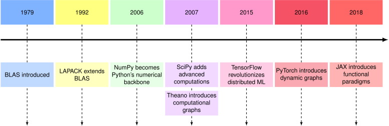](https://mlsysbook.ai/contents/core/frameworks/192c0bf590065201a107df4f3e5a3745ad474686.svg "Figure 1: Computational Library Evolution: Modern machine learning frameworks build upon decades of numerical computing advancements, transitioning from low-level routines like BLAS and LAPACK to high-level abstractions in numpy, scipy, and finally to deep learning frameworks such as TensorFlow and PyTorch. This progression reflects a shift toward increased developer productivity and accessibility in machine learning system development.")
Figure 1: **Computational Library Evolution**: Modern machine learning frameworks build upon decades of numerical computing advancements, transitioning from low-level routines like BLAS and LAPACK to high-level abstractions in numpy, scipy, and finally to deep learning frameworks such as TensorFlow and PyTorch. This progression reflects a shift toward increased developer productivity and accessibility in machine learning system development.
This progression demonstrates how frameworks achieve their capabilities through incremental innovation, building computational accessibility upon foundations established by their predecessors.
### Foundational Mathematical Computing Infrastructure
The foundation for modern ML frameworks begins at the core level of computation: matrix operations. Machine learning computations are primarily matrix-matrix and matrix-vector multiplications because neural networks process data through linear transformations[1](https://mlsysbook.ai/contents/core/frameworks/frameworks.html#fn1)
applied to multidimensional arrays. The Basic Linear Algebra Subprograms ([BLAS](https://www.netlib.org/blas/)
)[2](https://mlsysbook.ai/contents/core/frameworks/frameworks.html#fn2)
, developed in 1979, provided these essential matrix operations that would become the computational backbone of machine learning ([Kung and Leiserson 1979](https://mlsysbook.ai/contents/core/frameworks/frameworks.html#ref-kung1979systolic)
). These low-level operations, when combined and executed, enable the complex calculations required for training neural networks and other ML models.
1 **Linear Transformations**: Mathematical operations that preserve vector addition and scalar multiplication, typically implemented as matrix multiplication in neural networks. Each layer applies a learned linear transformation (weights matrix) followed by a non-linear activation function (like ReLU or sigmoid), enabling networks to learn complex patterns from simple mathematical building blocks.
2 **BLAS (Basic Linear Algebra Subprograms)**: Originally developed at Argonne National Laboratory, BLAS became the de facto standard for linear algebra operations, with Level 1 (vector-vector), Level 2 (matrix-vector), and Level 3 (matrix-matrix) operations that still underpin every modern ML framework.
Kung, Hsiang Tsung, and Charles E Leiserson. 1979. “Systolic Arrays (for VLSI).” In _Sparse Matrix Proceedings 1978_, 1:256–82. Society for industrial; applied mathematics Philadelphia, PA, USA.
3 **LAPACK (Linear Algebra Package)**: Succeeded LINPACK and EISPACK, introducing block algorithms that dramatically improved cache efficiency and parallel execution, innovations that became essential as datasets grew from megabytes to terabytes.
Building upon BLAS, the Linear Algebra Package ([LAPACK](https://www.netlib.org/lapack/)
)[3](https://mlsysbook.ai/contents/core/frameworks/frameworks.html#fn3)
emerged in 1992, extending these capabilities with advanced linear algebra operations such as matrix decompositions, eigenvalue problems, and linear system solutions. This layered approach of building increasingly complex operations from basic matrix computations became a defining characteristic of ML frameworks.
This foundation of optimized linear algebra operations set the stage for higher-level abstractions that would make numerical computing more accessible. The development of [NumPy](https://numpy.org/)
in 2006 marked an important milestone in this evolution, building upon its predecessors Numeric and Numarray to become the primary package for numerical computation in Python. NumPy introduced n-dimensional array objects and essential mathematical functions, providing an efficient interface to these underlying BLAS and LAPACK operations. This abstraction allowed developers to work with high-level array operations while maintaining the performance of optimized low-level matrix computations.
The trend continued with [SciPy](https://scipy.org/)
, which built upon NumPy’s foundations to provide specialized functions for optimization, linear algebra, and signal processing, with its first stable release in 2008. This layered architecture, progressing from basic matrix operations to numerical computations, established the blueprint for future ML frameworks.
### Early Machine Learning Platform Development
The next evolutionary phase represented a conceptual leap from general numerical computing to domain-specific machine learning tools. The transition from numerical libraries to dedicated machine learning frameworks marked an important evolution in abstraction. While the underlying computations remained rooted in matrix operations, frameworks began to encapsulate these operations into higher-level machine learning primitives. The University of Waikato introduced Weka in 1993 ([Witten and Frank 2002](https://mlsysbook.ai/contents/core/frameworks/frameworks.html#ref-witten2002data)
), one of the earliest ML frameworks, which abstracted matrix operations into data mining tasks, though it was limited by its Java implementation and focus on smaller-scale computations.
Witten, Ian H., and Eibe Frank. 2002. “Data Mining: Practical Machine Learning Tools and Techniques with Java Implementations.” _ACM SIGMOD Record_ 31 (1): 76–77. [https://doi.org/10.1145/507338.507355](https://doi.org/10.1145/507338.507355)
.
This paradigm shift became evident with [Scikit-learn](https://scikit-learn.org/stable/)
, emerging in 2007 as a significant advancement in machine learning abstraction. Building upon the NumPy and SciPy foundation, it transformed basic matrix operations into intuitive ML algorithms. For example, what amounts to a series of matrix multiplications and gradient computations became a simple `fit()` method call in a logistic regression model. This abstraction pattern, hiding complex matrix operations behind clean APIs, would become a defining characteristic of modern ML frameworks.
[Theano](https://github.com/Theano/Theano)
[4](https://mlsysbook.ai/contents/core/frameworks/frameworks.html#fn4)
, developed at the Montreal Institute for Learning Algorithms (MILA) and appearing in 2007, was a major advancement that introduced two revolutionary concepts: computational graphs[5](https://mlsysbook.ai/contents/core/frameworks/frameworks.html#fn5)
and GPU acceleration ([Team et al. 2016](https://mlsysbook.ai/contents/core/frameworks/frameworks.html#ref-al2016theano)
). Computational graphs represented mathematical operations as directed graphs, with matrix operations as nodes and data flowing between them. This graph-based approach allowed for automatic differentiation and optimization of the underlying matrix operations. More importantly, it enabled the framework to automatically route these operations to GPU hardware, dramatically accelerating matrix computations.
4 **Theano**: Named after the ancient Greek mathematician Theano of Croton, this framework pioneered the concept of symbolic mathematical expressions in Python, laying the groundwork for every modern deep learning framework.
5 **Computational Graphs**: First formalized in automatic differentiation literature by Wengert (1964), this representation became the backbone of modern ML frameworks, enabling both forward and reverse-mode differentiation at unprecedented scale.
Team, The Theano Development, Rami Al-Rfou, Guillaume Alain, Amjad Almahairi, Christof Angermueller, Dzmitry Bahdanau, Nicolas Ballas, et al. 2016. “Theano: A Python Framework for Fast Computation of Mathematical Expressions,” May. [http://arxiv.org/abs/1605.02688v1](http://arxiv.org/abs/1605.02688v1)
.
6 **Eager Execution**: An execution model where operations are evaluated immediately as they are called, similar to standard Python execution. Pioneered by Torch in 2002, this approach prioritizes developer productivity and debugging ease over performance optimization, becoming the default mode in modern frameworks like PyTorch and TensorFlow 2.x.
A parallel development track emerged with [Torch7](http://torch.ch/)
(the Lua-based predecessor to PyTorch), created at NYU in 2002, which took a different approach to handling matrix operations. It emphasized immediate execution of operations (eager execution[6](https://mlsysbook.ai/contents/core/frameworks/frameworks.html#fn6)
) and provided an adaptable interface for neural network implementations.
Torch’s design philosophy of prioritizing developer experience while maintaining high performance established design patterns that would later influence frameworks like PyTorch. Its architecture demonstrated how to balance high-level abstractions with efficient low-level matrix operations, introducing concepts that would prove crucial as deep learning complexity increased.
### Deep Learning Computational Platform Innovation
The emergence of deep learning created unprecedented computational demands that exposed the limitations of existing frameworks. The deep learning revolution required a major shift in how frameworks handled matrix operations, primarily due to three factors: the massive scale of computations, the complexity of gradient calculations through deep networks, and the need for distributed processing. Traditional frameworks, designed for classical machine learning algorithms, could not handle the billions of matrix operations required for training deep neural networks.
This computational challenge sparked innovation in academic research environments that would reshape framework development. The foundations for modern deep learning frameworks emerged from academic research. The University of Montreal’s [Theano](https://github.com/Theano/Theano)
, released in 2007, established the concepts that would shape future frameworks ([Bergstra et al. 2010](https://mlsysbook.ai/contents/core/frameworks/frameworks.html#ref-bergstra2010theano)
). It introduced key concepts such as computational graphs for automatic differentiation and GPU acceleration, demonstrating how to organize and optimize complex neural network computations.
Bergstra, James, Olivier Breuleux, Frédéric Bastien, Pascal Lamblin, Razvan Pascanu, Guillaume Desjardins, Joseph Turian, David Warde-Farley, and Yoshua Bengio. 2010. “Theano: A CPU and GPU Math Compiler in Python.” In _Proceedings of the 9th Python in Science Conference_, 4:18–24. 1. SciPy. [https://doi.org/10.25080/majora-92bf1922-003](https://doi.org/10.25080/majora-92bf1922-003)
.
Jia, Yangqing, Evan Shelhamer, Jeff Donahue, Sergey Karayev, Jonathan Long, Ross Girshick, Sergio Guadarrama, and Trevor Darrell. 2014. “Caffe: Convolutional Architecture for Fast Feature Embedding.” In _Proceedings of the 22nd ACM International Conference on Multimedia_, 675–78. ACM. [https://doi.org/10.1145/2647868.2654889](https://doi.org/10.1145/2647868.2654889)
.
[Caffe](https://caffe.berkeleyvision.org/)
, released by UC Berkeley in 2013, advanced this evolution by introducing specialized implementations of convolutional operations ([Jia et al. 2014](https://mlsysbook.ai/contents/core/frameworks/frameworks.html#ref-jia2014caffe)
). While convolutions are mathematically equivalent to specific patterns of matrix multiplication, Caffe optimized these patterns specifically for computer vision tasks, demonstrating how specialized matrix operation implementations could dramatically improve performance for specific network architectures.
The next breakthrough came from industry, where computational scale demands required new architectural approaches. Google’s [TensorFlow](https://www.tensorflow.org/)
[7](https://mlsysbook.ai/contents/core/frameworks/frameworks.html#fn7)
, introduced in 2015, revolutionized the field by treating matrix operations as part of a distributed computing problem ([Dean et al. 2012](https://mlsysbook.ai/contents/core/frameworks/frameworks.html#ref-dean2012large)
). It represented all computations, from individual matrix multiplications to entire neural networks, as a static computational graph[8](https://mlsysbook.ai/contents/core/frameworks/frameworks.html#fn8)
that could be split across multiple devices. This approach enabled training of unprecedented model sizes by distributing matrix operations across clusters of computers and specialized hardware. TensorFlow’s static graph approach, while initially constraining, allowed for aggressive optimization of matrix operations through techniques like kernel fusion[9](https://mlsysbook.ai/contents/core/frameworks/frameworks.html#fn9)
(combining multiple operations into a single kernel for efficiency) and memory planning[10](https://mlsysbook.ai/contents/core/frameworks/frameworks.html#fn10)
(pre-allocating memory for operations).
7 **TensorFlow**: Named after tensor operations flowing through computational graphs, this framework democratized distributed machine learning by open-sourcing Google’s internal DistBelief system, instantly giving researchers access to infrastructure that previously required massive corporate resources.
Dean, Jeffrey, Greg Corrado, Rajat Monga, Kai Chen 0010, Matthieu Devin, Quoc V. Le, Mark Z. Mao, et al. 2012. “Large Scale Distributed Deep Networks.” In _Advances in Neural Information Processing Systems 25: 26th Annual Conference on Neural Information Processing Systems 2012. Proceedings of a Meeting Held December 3-6, 2012, Lake Tahoe, Nevada, United States_, edited by Peter L. Bartlett, Fernando C. N. Pereira, Christopher J. C. Burges, Léon Bottou, and Kilian Q. Weinberger, 1232–40. [https://proceedings.neurips.cc/paper/2012/hash/6aca97005c68f1206823815f66102863-Abstract.html](https://proceedings.neurips.cc/paper/2012/hash/6aca97005c68f1206823815f66102863-Abstract.html)
.
8 **Static Computational Graph**: A pre-defined computation structure where the entire model architecture is specified before execution, enabling global optimizations and efficient memory planning. Pioneered by TensorFlow 1.x, this approach sacrifices runtime flexibility for maximum performance optimization, making it ideal for production deployments.
9 **Kernel Fusion**: An optimization technique that combines multiple separate operations (like matrix multiplication followed by bias addition and activation) into a single GPU kernel, reducing memory bandwidth requirements by up to 10x and eliminating intermediate memory allocations. This optimization is particularly crucial for complex deep learning models with thousands of operations.
10 **Memory Planning**: A framework optimization that pre-analyzes computational graphs to determine optimal memory allocation strategies, enabling techniques like in-place operations and memory reuse patterns that can reduce peak memory usage by 40-60% during training.
Seide, Frank, and Amit Agarwal. 2016. “CNTK: Microsoft’s Open-Source Deep-Learning Toolkit.” In _Proceedings of the 22nd ACM SIGKDD International Conference on Knowledge Discovery and Data Mining_, 2135–35. ACM. [https://doi.org/10.1145/2939672.2945397](https://doi.org/10.1145/2939672.2945397)
.
The deep learning framework ecosystem continued to diversify as distinct organizations addressed specific computational challenges. Microsoft’s [CNTK](https://learn.microsoft.com/en-us/cognitive-toolkit/)
entered the field in 2016, bringing implementations for speech recognition and natural language processing tasks ([Seide and Agarwal 2016](https://mlsysbook.ai/contents/core/frameworks/frameworks.html#ref-seide2016cntk)
). Its architecture emphasized scalability across distributed systems while maintaining efficient computation for sequence-based models.
Simultaneously, Facebook’s [PyTorch](https://pytorch.org/)
[11](https://mlsysbook.ai/contents/core/frameworks/frameworks.html#fn11)
, also launched in 2016, took a radically different approach to handling matrix computations. Instead of static graphs, PyTorch introduced dynamic computational graphs that could be modified on the fly ([Paszke et al. 2019](https://mlsysbook.ai/contents/core/frameworks/frameworks.html#ref-paszke2019pytorch)
). This dynamic approach, while potentially sacrificing optimization opportunities, simplified debugging and analysis of matrix operation flow in their models for researchers. PyTorch’s success demonstrated that the ability to introspect and modify computations dynamically was equally important as raw performance for research applications.
11 **PyTorch**: Inspired by the original Torch framework from NYU, PyTorch brought “define-by-run” semantics to Python, enabling researchers to modify models during execution, a breakthrough that accelerated research by making debugging as simple as using a standard Python debugger.
Paszke, Adam, Sam Gross, Francisco Massa, Adam Lerer, James Bradbury, Gregory Chanan, Trevor Killeen, et al. 2019. “PyTorch: An Imperative Style, High-Performance Deep Learning Library.” In _Advances in Neural Information Processing Systems_, 32:8024–35. [https://proceedings.neurips.cc/paper/2019/hash/bdbca288fee7f92f2bfa9f7012727740-Abstract.html](https://proceedings.neurips.cc/paper/2019/hash/bdbca288fee7f92f2bfa9f7012727740-Abstract.html)
.
Framework development continued to expand with Amazon’s [MXNet](https://mxnet.apache.org/)
, which approached the challenge of large-scale matrix operations by focusing on memory efficiency and scalability across different hardware configurations. It introduced a hybrid approach that combined aspects of both static and dynamic graphs, enabling adaptable model development while maintaining aggressive optimization of the underlying matrix operations.
These diverse approaches revealed that no single solution could address all deep learning requirements, leading to the development of specialized tools. As deep learning applications grew more diverse, the need for specialized and higher-level abstractions became apparent. [Keras](https://keras.io/)
emerged in 2015 to address this need, providing a unified interface that could run on top of multiple lower-level frameworks ([Chollet et al. 2015](https://mlsysbook.ai/contents/core/frameworks/frameworks.html#ref-chollet2015keras)
). This higher-level abstraction approach demonstrated how frameworks could focus on user experience while leveraging the computational power of existing systems.
Chollet, François et al. 2015. “Keras.” _GitHub Repository_. [https://github.com/fchollet/keras](https://github.com/fchollet/keras)
.
12 **JAX**: Stands for “Just After eXecution” and combines NumPy’s API with functional programming transforms (jit, grad, vmap, pmap), enabling researchers to write concise code that automatically scales to TPUs and GPU clusters while maintaining NumPy compatibility.
Bradbury, James, Roy Frostig, Peter Hawkins, Matthew James Johnson, Chris Leary, Dougal Maclaurin, George Necula, et al. 2018. “JAX: Composable Transformations of Python+NumPy Programs.” [http://github.com/google/jax](https://github.com/google/jax)
.
Howard, Jeremy, and Sylvain Gugger. 2020. “Fastai: A Layered API for Deep Learning.” _Information_ 11 (2): 108. [https://doi.org/10.3390/info11020108](https://doi.org/10.3390/info11020108)
.
Meanwhile, Google’s [JAX](https://github.com/google/jax)
[12](https://mlsysbook.ai/contents/core/frameworks/frameworks.html#fn12)
, introduced in 2018, brought functional programming principles to deep learning computations, enabling new patterns of model development ([Bradbury et al. 2018](https://mlsysbook.ai/contents/core/frameworks/frameworks.html#ref-jax2018github)
). [FastAI](https://www.fast.ai/)
built upon PyTorch to package common deep learning patterns into reusable components, making advanced techniques more accessible to practitioners ([Howard and Gugger 2020](https://mlsysbook.ai/contents/core/frameworks/frameworks.html#ref-howard2020fastai)
). These higher-level frameworks demonstrated how abstraction could simplify development while maintaining the performance benefits of their underlying implementations.
### Hardware-Driven Framework Architecture Evolution
The evolution of frameworks has been inextricably linked to advances in computational hardware, creating a dynamic relationship between software capabilities and hardware innovations. Hardware developments have significantly reshaped how frameworks implement and optimize matrix operations. The introduction of [NVIDIA’s CUDA platform](https://developer.nvidia.com/cuda-toolkit)
[13](https://mlsysbook.ai/contents/core/frameworks/frameworks.html#fn13)
in 2007 marked a critical moment in framework design by enabling general-purpose computing on GPUs ([Nickolls et al. 2008](https://mlsysbook.ai/contents/core/frameworks/frameworks.html#ref-nickolls2008scalable)
). This was transformative because GPUs excel at parallel matrix operations, offering orders of magnitude speedup for the computations in deep learning. While a CPU might process matrix elements sequentially, a GPU can process thousands of elements simultaneously, significantly changing how frameworks approach computation scheduling.
13 **CUDA (Compute Unified Device Architecture)**: NVIDIA’s parallel computing platform launched in 2007 that transformed ML by enabling general-purpose GPU computing. GPUs can execute thousands of threads simultaneously, providing 10-100x speedup for matrix operations compared to CPUs, fundamentally changing how ML frameworks approach computation scheduling.
Nickolls, John, Ian Buck, Michael Garland, and Kevin Skadron. 2008. “Scalable Parallel Programming with CUDA: Is CUDA the Parallel Programming Model That Application Developers Have Been Waiting For?” _Queue_ 6 (2): 40–53. [https://doi.org/10.1145/1365490.1365500](https://doi.org/10.1145/1365490.1365500)
.
Modern GPU architectures demonstrate quantifiable efficiency advantages for ML workloads. NVIDIA A100 GPUs provide 312 TFLOPS of tensor operations at FP16 precision with 1.6 TB/s memory bandwidth, compared to typical CPU configurations delivering 1-2 TFLOPS with 50-100 GB/s memory bandwidth. These hardware characteristics significantly change framework optimization strategies. Frameworks must design computational graphs that maximize GPU utilization by ensuring sufficient computational intensity (measured in FLOPS per byte transferred) to saturate the available memory bandwidth.
Memory bandwidth optimization becomes critical when frameworks target GPU acceleration. The memory bandwidth-to-compute ratio (bytes per FLOP) determines whether operations are compute-bound or memory-bound. Matrix multiplication operations with large dimensions (typically N×N where N > 1024) achieve high computational intensity and become compute-bound, enabling near-peak GPU utilization. However, element-wise operations like activation functions frequently become memory-bound, achieving only 10-20% of peak performance. Frameworks address this through operator fusion techniques, combining memory-bound operations into single kernels that reduce memory transfers.
Beyond general GPU acceleration, the development of hardware-specific accelerators further revolutionized framework design. [Google’s Tensor Processing Units (TPUs)](https://cloud.google.com/tpu/)
[14](https://mlsysbook.ai/contents/core/frameworks/frameworks.html#fn14)
, first deployed in 2016, were purpose-built for tensor operations, the essential building blocks of deep learning computations. TPUs introduced systolic array[15](https://mlsysbook.ai/contents/core/frameworks/frameworks.html#fn15)
architectures, which are particularly efficient for matrix multiplication and convolution operations. This hardware architecture prompted frameworks like TensorFlow to develop specialized compilation strategies that could map high-level operations directly to TPU instructions, bypassing traditional CPU-oriented optimizations.
14 **TPU (Tensor Processing Unit)**: Google’s first-generation TPU (v1) achieved 15-30x better performance-per-watt than contemporary GPUs and CPUs for neural networks, proving that domain-specific architectures could outperform general-purpose processors for ML workloads.
15 **Systolic Array**: A specialized parallel computing architecture invented by H.T. Kung (CMU) and Charles Leiserson (MIT) in 1978, where data flows through a grid of processing elements in a rhythmic, pipeline fashion. Each element performs simple operations on data flowing from neighbors, making it exceptionally efficient for matrix operations, which form the heart of neural network computations.
TPU architecture demonstrates specialized efficiency gains through quantitative metrics. TPU v4 chips achieve 275 TFLOPS of BF16 compute with 1.2 TB/s memory bandwidth while consuming 200W power, delivering 1.375 TFLOPS/W power efficiency. This represents a 3-5x energy efficiency improvement over contemporary GPUs for large matrix operations. However, TPUs optimize specifically for dense matrix operations and show reduced efficiency for sparse computations or operations requiring complex control flow. Frameworks targeting TPUs must design computational graphs that maximize dense matrix operation usage while minimizing data movement between on-chip high-bandwidth memory (32 GB at 1.2 TB/s) and off-chip memory.
Mobile hardware accelerators, such as [Apple’s Neural Engine (2017)](https://machinelearning.apple.com/research/neural-engine)
and Qualcomm’s Neural Processing Units, brought new constraints and opportunities to framework design. These devices emphasized power efficiency over raw computational speed, requiring frameworks to develop new strategies for quantization and operator fusion. Mobile frameworks like TensorFlow Lite (more recently rebranded to [LiteRT](https://ai.google.dev/edge/litert)
) and [PyTorch Mobile](https://pytorch.org/mobile/home/)
needed to balance model accuracy with energy consumption, leading to innovations in how matrix operations are scheduled and executed.
Mobile accelerators demonstrate the critical importance of mixed-precision computation for energy efficiency. Apple’s Neural Engine in the A17 Pro chip provides 35 TOPS (trillion operations per second) of INT8 performance while consuming approximately 5W, achieving 7.2 TOPS/W efficiency. This represents a 10-15x energy efficiency improvement over FP32 computation on the same chip. Frameworks targeting mobile hardware must provide automatic mixed-precision policies that determine optimal precision for each operation, balancing energy consumption against accuracy degradation.
Sparse computation frameworks address the memory bandwidth limitations of mobile hardware. Sparse neural networks can reduce memory traffic by 50-90% for networks with structured sparsity patterns, directly improving energy efficiency since memory access consumes 10-100x more energy than arithmetic operations on mobile processors. Frameworks like Neural Magic’s SparseML automatically generate sparse models that maintain accuracy while conforming to hardware sparsity support. Qualcomm’s Neural Processing SDK provides specialized kernels for 2:4 structured sparse operations, where 2 out of every 4 consecutive weights are zero, enabling 1.5-2x speedup with minimal accuracy loss.
The emergence of custom ASIC[16](https://mlsysbook.ai/contents/core/frameworks/frameworks.html#fn16)
(Application-Specific Integrated Circuit) solutions has further diversified the hardware landscape. Companies like [Graphcore](https://www.graphcore.ai/)
, [Cerebras](https://www.cerebras.net/)
, and [SambaNova](https://sambanova.ai/)
have developed unique architectures for matrix computation, each with different strengths and optimization opportunities. This growth in specialized hardware has driven frameworks to adopt more adaptable intermediate representations[17](https://mlsysbook.ai/contents/core/frameworks/frameworks.html#fn17)
of matrix operations, enabling target-specific optimization while maintaining a common high-level interface.
16 **ASIC (Application-Specific Integrated Circuit)**: Custom silicon chips designed for specific tasks, contrasting with general-purpose CPUs. In ML contexts, ASICs like Google’s TPUs and Tesla’s FSD chips sacrifice flexibility for 10-100x efficiency gains in matrix operations, though they require 2-4 years development time and millions in upfront costs.
17 **Intermediate Representation (IR)**: A framework-internal format that sits between high-level user code and hardware-specific machine code, enabling optimizations and cross-platform deployment. Modern ML frameworks use IRs like TensorFlow’s XLA or PyTorch’s TorchScript to compile the same model for CPUs, GPUs, TPUs, and mobile devices.
The emergence of reconfigurable hardware added another layer of complexity and opportunity. Field Programmable Gate Arrays (FPGAs) introduced yet another dimension to framework optimization. Unlike fixed-function ASICs, FPGAs allow for reconfigurable circuits that can be optimized for specific matrix operation patterns. Frameworks responding to this capability developed just-in-time compilation strategies that could generate optimized hardware configurations based on the specific needs of a model.
This hardware-driven evolution demonstrates how framework design must constantly adapt to leverage new computational capabilities. Having traced how frameworks evolved from simple numerical libraries to platforms driven by hardware innovations, we now turn to understanding the core concepts that enable modern frameworks to manage this computational complexity. These key concepts (computational graphs, execution models, and system architectures) form the foundation upon which all framework capabilities are built.
**Self-Check: Question 1.2**
1. Which of the following frameworks introduced the concept of computational graphs and GPU acceleration, significantly advancing ML framework capabilities?
1. Weka
2. NumPy
3. Scikit-learn
4. Theano
2. Explain how the introduction of NVIDIA’s CUDA platform in 2007 influenced the design of ML frameworks.
3. Order the following ML frameworks based on their introduction timeline: (1) TensorFlow, (2) NumPy, (3) PyTorch, (4) BLAS.
4. What was a key advantage of PyTorch’s dynamic computational graphs over TensorFlow’s static graphs?
1. Simplified debugging and model modification
2. Higher performance optimization
3. Better support for distributed computing
4. Lower memory usage
[See Answers →](https://mlsysbook.ai/contents/core/frameworks/frameworks.html#quiz-answer-sec-ai-frameworks-historical-development-trajectory-9519)
Fundamental Concepts
--------------------
Modern machine learning frameworks operate through the integration of four key layers: Fundamentals, Data Handling, Developer Interface, and Execution and Abstraction. These layers function together to provide a structured and efficient foundation for model development and deployment, as illustrated in [Figure 2](https://mlsysbook.ai/contents/core/frameworks/frameworks.html#fig-fm_blocks)
.
[](https://mlsysbook.ai/contents/core/frameworks/aec05a548b44fdacd94cab43040d6569f2b2b7f5.svg "Figure 2: Framework Layer Interaction: Modern machine learning frameworks organize functionality into distinct layers (fundamentals, data handling, developer interface, and execution & abstraction) that collaborate to streamline model building and deployment. This layered architecture enables modularity and allows developers to focus on specific aspects of the machine learning workflow without needing to manage low-level infrastructure.")
Figure 2: **Framework Layer Interaction**: Modern machine learning frameworks organize functionality into distinct layers (fundamentals, data handling, developer interface, and execution & abstraction) that collaborate to streamline model building and deployment. This layered architecture enables modularity and allows developers to focus on specific aspects of the machine learning workflow without needing to manage low-level infrastructure.
The Fundamentals layer establishes the structural basis of these frameworks through computational graphs. These graphs use the directed acyclic graph (DAG) representation, enabling automatic differentiation and optimization. By organizing operations and data dependencies, computational graphs provide the framework with the ability to distribute workloads and execute computations across a variety of hardware platforms.
Building upon this structural foundation, the Data Handling layer manages numerical data and parameters essential for machine learning workflows. Central to this layer are specialized data structures, such as tensors, which handle high-dimensional arrays while optimizing memory usage and device placement. Memory management and data movement strategies ensure that computational workloads are executed effectively, particularly in environments with diverse or limited hardware resources.
The Developer Interface layer provides the tools and abstractions through which users interact with the framework. Programming models allow developers to define machine learning algorithms in a manner suited to their specific needs. These are categorized as either imperative or symbolic. Imperative models offer flexibility and ease of debugging, while symbolic models prioritize performance and deployment efficiency. Execution models further shape this interaction by defining whether computations are carried out eagerly (immediately) or as pre-optimized static graphs.
At the bottom of this architectural stack, the Execution and Abstraction layer transforms these high-level representations into efficient hardware-executable operations. Core operations, encompassing everything from basic linear algebra to complex neural network layers, are optimized for diverse hardware platforms. This layer also includes mechanisms for allocating resources and managing memory dynamically, ensuring scalable performance in both training and inference settings.
These four layers work together through carefully designed interfaces and dependencies, creating a cohesive system that balances usability with performance. Understanding these interconnected layers is essential for leveraging machine learning frameworks effectively. Each layer plays a distinct yet interdependent role in facilitating experimentation, optimization, and deployment. By mastering these concepts, practitioners can make informed decisions about resource utilization, scaling strategies, and the suitability of specific frameworks for various tasks.
Our exploration begins with computational graphs because they form the structural foundation that enables all other framework capabilities. This core abstraction provides the mathematical representation underlying automatic differentiation, optimization, and hardware acceleration capabilities that distinguish modern frameworks from simple numerical libraries.
### Computational Graphs
The computational graph is the central abstraction that enables frameworks to transform intuitive model descriptions into efficient hardware execution. This representation organizes mathematical operations and their dependencies to enable automatic optimization, parallelization, and hardware specialization.
#### Computational Graph Fundamentals
Computational graphs emerged as a key abstraction in machine learning frameworks to address the growing complexity of deep learning models. As models grew larger and more complex, efficient execution across diverse hardware platforms became necessary. The computational graph transforms high-level model descriptions into efficient low-level hardware execution ([Baydin et al. 2017](https://mlsysbook.ai/contents/core/frameworks/frameworks.html#ref-baydin2018)
), representing a machine learning model as a directed acyclic graph[18](https://mlsysbook.ai/contents/core/frameworks/frameworks.html#fn18)
(DAG) where nodes represent operations and edges represent data flow. This DAG abstraction enables automatic differentiation and efficient optimization across diverse hardware platforms.
18 **Directed Acyclic Graph (DAG)**: In machine learning frameworks, DAGs represent computation where nodes are operations (like matrix multiplication or activation functions) and edges are data dependencies. Unlike general DAGs in computer science, ML computational graphs specifically optimize for automatic differentiation, enabling frameworks to compute gradients by traversing the graph in reverse order.
For example, a node might represent a matrix multiplication operation, taking two input matrices (or tensors) and producing an output matrix (or tensor). To visualize this, consider the simple example in [Figure 3](https://mlsysbook.ai/contents/core/frameworks/frameworks.html#fig-comp-graph)
. The directed acyclic graph computes \\(z = x \\times y\\), where each variable is just numbers.
[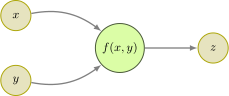](https://mlsysbook.ai/contents/core/frameworks/8de4c63fb10f7b924d681363ba33217504e7402e.svg "Figure 3: Computational Graph: Directed acyclic graphs represent machine learning models as a series of interconnected operations, enabling efficient computation and automatic differentiation. This example presents a simple computation, z = x \times y, where nodes define operations and edges specify the flow of data between them.")
Figure 3: **Computational Graph**: Directed acyclic graphs represent machine learning models as a series of interconnected operations, enabling efficient computation and automatic differentiation. This example presents a simple computation, \\(z = x \\times y\\), where nodes define operations and edges specify the flow of data between them.
This simple example illustrates the fundamental principle, but real machine learning models require much more complex graph structures. As shown in [Figure 4](https://mlsysbook.ai/contents/core/frameworks/frameworks.html#fig-mlfm-comp-graph)
, the structure of the computation graph involves defining interconnected layers, such as convolution, activation, pooling, and normalization, which are optimized before execution. The figure also demonstrates key system-level interactions, including memory management and device placement, showing how the static graph approach enables complete pre-execution analysis and resource allocation.
[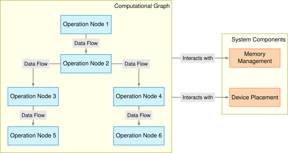](https://mlsysbook.ai/contents/core/frameworks/4d64429f98884a93daf67a671fb763bfd59d627b.svg "Figure 4: Computation Graph: This diagram represents a computation as a directed acyclic graph, where nodes denote variables and edges represent operations. By expressing computations in this form, systems can efficiently perform automatic differentiation, which is essential for training machine learning models through gradient-based optimization, and optimize resource allocation before execution.")
Figure 4: **Computation Graph**: This diagram represents a computation as a directed acyclic graph, where nodes denote variables and edges represent operations. By expressing computations in this form, systems can efficiently perform automatic differentiation, which is essential for training machine learning models through gradient-based optimization, and optimize resource allocation before execution.
##### Layers and Tensors
Modern machine learning frameworks implement neural network computations through two key abstractions: layers and tensors. Layers represent computational units that perform operations like convolution, pooling, or dense transformations. Each layer maintains internal states, including weights and biases, that evolve during model training. When data flows through these layers, it takes the form of tensors, immutable mathematical objects that hold and transmit numerical values.
The relationship between layers and tensors mirrors the distinction between operations and data in traditional programming. A layer defines how to transform input tensors into output tensors, much like a function defines how to transform its inputs into outputs. However, layers add an extra dimension: they maintain and update internal parameters during training. For example, a convolutional layer not only specifies how to perform convolution operations but also learns and stores the optimal convolution filters for a given task.
This abstraction becomes particularly powerful when frameworks automate the graph construction process. When a developer writes `tf.keras.layers.Conv2D`, the framework constructs the necessary graph nodes for convolution operations, parameter management, and data flow, shielding developers from implementation complexities.
##### Neural Network Construction
The power of computational graphs extends beyond basic layer operations. Activation functions, essential for introducing non-linearity in neural networks, become nodes in the graph. Functions like ReLU, sigmoid, and tanh transform the output tensors of layers, enabling networks to approximate complex mathematical functions. Frameworks provide optimized implementations of these activation functions, allowing developers to experiment with different non-linearities without worrying about implementation details.
Modern frameworks extend this modular approach by providing complete model architectures as pre-configured computational graphs. Models like ResNet and MobileNet come ready to use, allowing developers to customize specific layers and leverage transfer learning from pre-trained weights.
##### System-Level Consequences
Using the computational graph abstraction established earlier, frameworks can analyze and optimize entire computations before execution begins. The explicit representation of data dependencies enables automatic differentiation for gradient-based optimization.
Beyond optimization capabilities, this graph structure also provides flexibility in execution. The same model definition can run efficiently across different hardware platforms, from CPUs to GPUs to specialized accelerators. The framework handles the complexity of mapping operations to specific hardware capabilities, optimizing memory usage, and coordinating parallel execution. The graph structure also enables model serialization, allowing trained models to be saved, shared, and deployed across different environments.
These system benefits distinguish computational graphs from simpler visualization tools. While neural network diagrams help visualize model architecture, computational graphs serve a deeper purpose. They provide the precise mathematical representation needed to transform intuitive model design into efficient execution. Understanding this representation reveals how frameworks transform high-level model descriptions into optimized, hardware-specific implementations, making modern deep learning practical at scale.
It is important to differentiate computational graphs from neural network diagrams, such as those for multilayer perceptrons (MLPs), which depict nodes and layers. Neural network diagrams visualize the architecture and flow of data through nodes and layers, providing an intuitive understanding of the model’s structure. In contrast, computational graphs provide a low-level representation of the underlying mathematical operations and data dependencies required to implement and train these networks.
These representational capabilities have far-reaching implications for framework design and performance. From a systems perspective, computational graphs provide several key capabilities that influence the entire machine learning pipeline. They enable automatic differentiation, which we will examine next, provide clear structure for analyzing data dependencies and potential parallelism, and serve as an intermediate representation that can be optimized and transformed for different hardware targets. However, the power of computational graphs depends critically on how and when they are executed, which brings us to the fundamental distinction between static and dynamic graph execution models.
#### Pre-Defined Computational Structure
Static computation graphs, pioneered by early versions of TensorFlow, implement a “define-then-run” execution model. In this approach, developers must specify the entire computation graph before execution begins. This architectural choice has significant implications for both system performance and development workflow, as we will examine later.
A static computation graph implements a clear separation between the definition of operations and their execution. During the definition phase, each mathematical operation, variable, and data flow connection is explicitly declared and added to the graph structure. This graph is a complete specification of the computation but does not perform any actual calculations. Instead, the framework constructs an internal representation of all operations and their dependencies, which will be executed in a subsequent phase.
This upfront definition enables powerful system-level optimizations. The framework can analyze the complete structure to identify opportunities for operation fusion, eliminating unnecessary intermediate results and reducing memory traffic by 3-10x through kernel fusion. Memory requirements can be precisely calculated and optimized in advance, leading to efficient allocation strategies. Static graphs enable compilation frameworks like XLA[19](https://mlsysbook.ai/contents/core/frameworks/frameworks.html#fn19)
(Accelerated Linear Algebra) to perform aggressive optimizations. Graph rewriting can eliminate substantial numbers of redundant operations while hardware-specific kernel generation can provide significant speedups over generic implementations. This abstraction, while elegant, imposes fundamental constraints on expressible computations: static graphs achieve these performance gains by sacrificing flexibility in control flow and dynamic computation patterns. Once validated, the same computation can be run repeatedly with high confidence in its behavior and performance characteristics.
19 **XLA (Accelerated Linear Algebra)**: TensorFlow’s domain-specific compiler that optimizes tensor operations for CPUs, GPUs, and TPUs. Achieves 3-10x speedups through operation fusion, memory layout optimization, and hardware-specific code generation, demonstrating how ML workloads benefit from specialized compilation strategies.
[Figure 5](https://mlsysbook.ai/contents/core/frameworks/frameworks.html#fig-mlfm-static-graph)
illustrates this fundamental two-phase approach: first, the complete computational graph is constructed and optimized; then, during the execution phase, actual data flows through the graph to produce results. This separation enables the framework to perform thorough analysis and optimization of the entire computation before any execution begins.
[](https://mlsysbook.ai/contents/core/frameworks/d9504b9e114aa7738e92044e5eb3199608865c4a.svg "Figure 5: Static Computation Graph: Machine learning frameworks first define computations as a graph of operations, enabling global optimizations like operation fusion and efficient resource allocation before any data flows through the system. This two-phase approach separates graph construction and optimization from execution, improving performance and predictability.")
Figure 5: **Static Computation Graph**: Machine learning frameworks first define computations as a graph of operations, enabling global optimizations like operation fusion and efficient resource allocation before any data flows through the system. This two-phase approach separates graph construction and optimization from execution, improving performance and predictability.
#### Runtime-Adaptive Computational Structure
Dynamic computation graphs, popularized by PyTorch, implement a “define-by-run” execution model. This approach constructs the graph during execution, offering greater flexibility in model definition and debugging. Unlike static graphs, which rely on predefined memory allocation, dynamic graphs allocate memory as operations execute, making them susceptible to memory fragmentation in long-running tasks. While dynamic graphs trade efficiency for flexibility in expressing control flow, they significantly limit compiler optimization opportunities. The inability to analyze the complete computation before execution prevents aggressive kernel fusion and graph rewriting optimizations that static graphs enable.
As shown in [Figure 6](https://mlsysbook.ai/contents/core/frameworks/frameworks.html#fig-mlfm-dynamic-graph-flow)
, each operation is defined, executed, and completed before moving on to define the next operation. This contrasts sharply with static graphs, where all operations must be defined upfront. When an operation is defined, it is immediately executed, and its results become available for subsequent operations or for inspection during debugging. This cycle continues until all operations are complete.
[](https://mlsysbook.ai/contents/core/frameworks/126eb7310926807c4e6d798196330c47db92dd15.svg "Figure 6: Dynamic Graph Execution: Machine learning frameworks define and execute operations sequentially at runtime, enabling flexible model construction and immediate evaluation of intermediate results. This contrasts with static graphs which require complete upfront definition, and supports debugging and adaptive computation during model training and inference.")
Figure 6: **Dynamic Graph Execution**: Machine learning frameworks define and execute operations sequentially at runtime, enabling flexible model construction and immediate evaluation of intermediate results. This contrasts with static graphs which require complete upfront definition, and supports debugging and adaptive computation during model training and inference.
Dynamic graphs excel in scenarios that require conditional execution or dynamic control flow, such as when processing variable-length sequences or implementing complex branching logic. They provide immediate feedback during development, making it easier to identify and fix issues in the computational pipeline. This flexibility aligns naturally with imperative programming patterns familiar to most developers, allowing them to inspect and modify computations at runtime. These characteristics make dynamic graphs particularly valuable during the research and development phase of ML projects.
#### Framework Architecture Trade-offs
The architectural differences between static and dynamic computational graphs have multiple implications for how machine learning systems are designed and executed. These implications touch on various aspects of memory usage, device utilization, execution optimization, and debugging, all of which play important roles in determining the efficiency and scalability of a system. We focus on memory management and device placement as foundational concepts, with optimization techniques covered in detail in **[Chapter 8: AI Training](https://mlsysbook.ai/contents/core/training/training.html#sec-ai-training)
**. This allows us to build a clear understanding before exploring more complex topics like optimization and fault tolerance.
##### Memory Management
Memory management occurs when executing computational graphs. Static graphs benefit from their predefined structure, allowing for precise memory planning before execution. Frameworks can calculate memory requirements in advance, optimize allocation, and minimize overhead through techniques like memory reuse. This structured approach helps ensure consistent performance, particularly in resource-constrained environments, such as Mobile and Tiny ML systems. For large models, frameworks must efficiently handle memory bandwidth requirements that can range from 100GB/s for smaller models to over 1TB/s for large language models with billions of parameters, making memory planning critical for achieving optimal throughput.
Dynamic graphs, by contrast, allocate memory dynamically as operations are executed. While this flexibility is invaluable for handling dynamic control flows or variable input sizes, it can result in higher memory overhead and fragmentation. These trade-offs are often most apparent during development, where dynamic graphs enable rapid iteration and debugging but may require additional optimization for production deployment. The dynamic allocation overhead becomes particularly significant when memory bandwidth utilization drops below 50% of available capacity due to fragmentation and suboptimal access patterns.
##### Device Placement
Device placement, the process of assigning operations to hardware resources such as CPUs, GPUs, or specialized ASICS like TPUs, is another system-level consideration. Static graphs allow for detailed pre-execution analysis, enabling the framework to map computationally intensive operations to devices while minimizing communication overhead. This capability makes static graphs well-suited for optimizing execution on specialized hardware, where performance gains can be significant.
Dynamic graphs, in contrast, handle device placement at runtime. This allows them to adapt to changing conditions, such as hardware availability or workload demands. However, the lack of a complete graph structure before execution can make it challenging to optimize device utilization fully, potentially leading to inefficiencies in large-scale or distributed setups.
##### Broader Perspective
The trade-offs between static and dynamic graphs extend well beyond memory and device considerations. As shown in [Table 1](https://mlsysbook.ai/contents/core/frameworks/frameworks.html#tbl-mlfm-graphs)
, these architectures influence optimization potential, debugging capabilities, scalability, and deployment complexity. These broader implications are explored in detail in **[Chapter 8: AI Training](https://mlsysbook.ai/contents/core/training/training.html#sec-ai-training)
** for training workflows and **[Chapter 11: AI Acceleration](https://mlsysbook.ai/contents/core/hw_acceleration/hw_acceleration.html#sec-ai-acceleration)
** for system-level optimizations.
These hybrid solutions aim to provide the flexibility of dynamic graphs during development while enabling the performance optimizations of static graphs in production environments. The choice between static and dynamic graphs often depends on specific project requirements, balancing factors like development speed, production performance, and system complexity.
Table 1: **Graph Computation Modes**: Static graphs define the entire computation upfront, enabling optimization, while dynamic graphs construct the computation on-the-fly, offering flexibility for variable-length inputs and control flow. This distinction impacts both the efficiency of execution and the ease of model development and debugging.
| | | |
| --- | --- | --- |
| **Memory Management** | Precise allocation planning, optimized memory usage | Flexible but likely less efficient allocation |
| **Optimization Potential** | Comprehensive graph-level optimizations possible | Limited to local optimizations due to runtime |
| **Hardware Utilization** | Can generate highly optimized hardware-specific code | May sacrifice hardware-specific optimizations |
| **Development Experience** | Requires more upfront planning, harder to debug | Better debugging, faster iteration cycles |
| **Debugging Workflow** | Framework-specific tools, disconnected stack traces | Standard Python debugging (pdb, print, inspect) |
| **Error Reporting** | Execution-time errors disconnected from definition | Intuitive stack traces pointing to exact lines |
| **Research Velocity** | Slower iteration due to define-then-run requirement | Faster prototyping and model experimentation |
| **Runtime Flexibility** | Fixed computation structure | Can adapt to runtime conditions |
| **Production Performance** | Generally better performance at scale | May have overhead from graph construction |
| **Integration with Legacy Code** | More separation between definition and execution | Natural integration with imperative code |
| **Memory Overhead** | Lower memory overhead due to planned allocations | Higher overhead due to dynamic allocations |
| **Deployment Complexity** | Simpler deployment due to fixed structure | May require additional runtime support |
#### Graph-Based Gradient Computation Implementation
The computational graph serves as more than just an execution plan; it is the core data structure that makes reverse-mode automatic differentiation feasible and efficient. Understanding this connection reveals how frameworks compute gradients through arbitrarily complex neural networks.
During the forward pass, the framework constructs a computational graph where each node represents an operation and stores both the result and the information needed to compute gradients. This graph is not just a visualization tool but an actual data structure maintained in memory. When `loss.backward()` is called, the framework performs a reverse traversal of this graph in reverse topological order, systematically applying the chain rule at each node.
The key insight is that the graph structure encodes all the dependency relationships needed for the chain rule. Each edge in the graph represents a partial derivative, and reverse traversal automatically composes these partial derivatives according to the chain rule. The forward pass builds the computation history, and the backward pass is simply a graph traversal algorithm that accumulates gradients by following the recorded dependencies.
This design enables automatic differentiation to scale to networks with millions of parameters because the complexity is linear in the number of operations, not exponential in the number of variables. The graph structure ensures that each gradient computation is performed exactly once and that shared subcomputations are properly handled through the dependency tracking built into the graph representation.
### Automatic Differentiation
Machine learning frameworks must solve a core computational challenge: calculating derivatives through complex chains of mathematical operations accurately and efficiently. This capability enables the training of neural networks by computing how millions of parameters require adjustment to improve the model’s performance ([Baydin et al. 2017](https://mlsysbook.ai/contents/core/frameworks/frameworks.html#ref-baydin2018)
).
Baydin, Atilim Gunes, Barak A. Pearlmutter, Alexey Andreyevich Radul, and Jeffrey Mark Siskind. 2017. “Automatic Differentiation in Machine Learning: A Survey.” _J. Mach. Learn. Res._ 18 (153): 153:1–43. [https://jmlr.org/papers/v18/17-468.html](https://jmlr.org/papers/v18/17-468.html)
.
[Listing 1](https://mlsysbook.ai/contents/core/frameworks/frameworks.html#lst-auto_diff_intro)
shows a simple computation that illustrates this challenge.
Listing 1: **Automatic Differentiation**: Enables efficient computation of gradients for complex functions, crucial for optimizing neural network parameters.
def f(x):
a = x * x # Square
b = sin(x) # Sine
return a * b # Product
Even in this basic example, computing derivatives manually would require careful application of calculus rules - the product rule, the chain rule, and derivatives of trigonometric functions. Now imagine scaling this to a neural network with millions of operations. This is where automatic differentiation (AD)[20](https://mlsysbook.ai/contents/core/frameworks/frameworks.html#fn20)
becomes essential.
20 **Automatic Differentiation**: Invented by Robert Edwin Wengert in 1964, this technique achieves machine precision derivatives by applying the chain rule at the elementary operation level, making neural network training computationally feasible for networks with millions of parameters.
Automatic differentiation calculates derivatives of functions implemented as computer programs by decomposing them into elementary operations. In our example, AD breaks down `f(x)` into three basic steps:
1. Computing `a = x * x` (squaring)
2. Computing `b = sin(x)` (sine function)
3. Computing the final product `a * b`
For each step, AD knows the basic derivative rules:
* For squaring: `d(x²)/dx = 2x`
* For sine: `d(sin(x))/dx = cos(x)`
* For products: `d(uv)/dx = u(dv/dx) + v(du/dx)`
By tracking how these operations combine and systematically applying the chain rule, AD computes exact derivatives through the entire computation. When implemented in frameworks like PyTorch or TensorFlow, this enables automatic computation of gradients through arbitrary neural network architectures, which becomes essential for the training algorithms and optimization techniques detailed in **[Chapter 8: AI Training](https://mlsysbook.ai/contents/core/training/training.html#sec-ai-training)
**. This fundamental understanding of how AD decomposes and tracks computations sets the foundation for examining its implementation in machine learning frameworks. We will explore its mathematical principles, system architecture implications, and performance considerations that make modern machine learning possible.
#### Forward and Reverse Mode Differentiation
Automatic differentiation can be implemented using two primary computational approaches, each with distinct characteristics in terms of efficiency, memory usage, and applicability to different problem types. This section examines forward mode and reverse mode automatic differentiation, analyzing their mathematical foundations, implementation structures, performance characteristics, and integration patterns within machine learning frameworks.
##### Forward Mode
Forward mode automatic differentiation computes derivatives alongside the original computation, tracking how changes propagate from input to output. Building on the basic AD concepts introduced in [Section 1.3.2](https://mlsysbook.ai/contents/core/frameworks/frameworks.html#sec-ai-frameworks-automatic-differentiation-e286)
, forward mode mirrors manual derivative computation, making it intuitive to understand and implement.
Consider our previous example with a slight modification to show how forward mode works (see [Listing 2](https://mlsysbook.ai/contents/core/frameworks/frameworks.html#lst-forward_mode_ad)
).
Listing 2: **Forward Mode Automatic Differentiation**: Computes derivatives alongside function evaluations using the product rule, illustrating how changes in inputs propagate to outputs.
def f(x): # Computing both value and derivative
# Step 1: x -> x²
a = x * x # Value: x²
da = 2 * x # Derivative: 2x
# Step 2: x -> sin(x)
b = sin(x) # Value: sin(x)
db = cos(x) # Derivative: cos(x)
# Step 3: Combine using product rule
result = a * b # Value: x² * sin(x)
dresult = a * db + b * da # Derivative: x²*cos(x) + sin(x)*2x
return result, dresult
Forward mode achieves this systematic derivative computation by augmenting each number with its derivative value, creating what mathematicians call a “dual number.” The example in [Listing 3](https://mlsysbook.ai/contents/core/frameworks/frameworks.html#lst-forward_mode_dual)
shows how this works numerically when x = 2.0, the computation tracks both values and derivatives:
Listing 3: **Forward Mode**: The example computes derivatives alongside function values using dual numbers, showcasing how to track changes in both the result and its rate of change.
x = 2.0 # Initial value
dx = 1.0 # We're tracking derivative with respect to x
# Step 1: x²
a = 4.0 # (2.0)²
da = 4.0 # 2 * 2.0
# Step 2: sin(x)
b = 0.909 # sin(2.0)
db = -0.416 # cos(2.0)
# Final result
result = 3.637 # 4.0 * 0.909
dresult = 2.805 # 4.0 * (-0.416) + 0.909 * 4.0
###### Implementation Structure
Forward mode AD structures computations to track both values and derivatives simultaneously through programs. The structure of such computations can be seen again in [Listing 4](https://mlsysbook.ai/contents/core/frameworks/frameworks.html#lst-forward_structure)
, where each intermediate operation is made explicit.
Listing 4: **Forward Mode AD Structure**: Each operation tracks values and derivatives simultaneously, highlighting how computations are structured in forward mode automatic differentiation.
def f(x):
a = x * x
b = sin(x)
return a * b
When a framework executes this function in forward mode, it augments each computation to carry two pieces of information: the value itself and how that value changes with respect to the input. This paired movement of value and derivative mirrors how we think about rates of change as shown in [Listing 5](https://mlsysbook.ai/contents/core/frameworks/frameworks.html#lst-dual_tracking)
.
Listing 5: **Dual Tracking**: Each computation tracks both its value and derivative, illustrating how forward mode automatic differentiation works in practice. This example helps understand how values and their rates of change are simultaneously computed during function evaluation.
# Conceptually, each computation tracks (value, derivative)
x = (2.0, 1.0) # Input value and its derivative
a = (4.0, 4.0) # x² and its derivative 2x
b = (0.909, -0.416) # sin(x) and its derivative cos(x)
result = (3.637, 2.805) # Final value and derivative
This forward propagation of derivative information happens automatically within the framework’s computational machinery. The framework: 1. Enriches each value with derivative information 2. Transforms each basic operation to handle both value and derivative 3. Propagates this information forward through the computation
The beauty of this approach is that it follows the natural flow of computation - as values move forward through the program, their derivatives move with them. This makes forward mode particularly well-suited for functions with single inputs and multiple outputs, as the derivative information follows the same path as the regular computation.
###### Performance Characteristics
Forward mode AD exhibits distinct performance patterns that influence when and how frameworks employ it. Understanding these characteristics helps explain why frameworks choose different AD approaches for different scenarios.
Forward mode performs one derivative computation alongside each original operation. For a function with one input variable, this means roughly doubling the computational work - once for the value, once for the derivative. The cost scales linearly with the number of operations in the program, making it predictable and manageable for simple computations.
However, consider a neural network layer computing derivatives for matrix multiplication between weights and inputs. To compute derivatives with respect to all weights, forward mode would require performing the computation once for each weight parameter, potentially thousands of times. This reveals an important characteristic: forward mode’s efficiency depends on the number of input variables we need derivatives for.
Forward mode’s memory requirements are relatively modest. It needs to store the original value, a single derivative value, and temporary results during computation. The memory usage stays constant regardless of how complex the computation becomes. This predictable memory pattern makes forward mode particularly suitable for embedded systems with limited memory, real-time applications requiring consistent memory use, and systems where memory bandwidth is a bottleneck.
This combination of computational scaling with input variables but constant memory usage creates specific trade-offs that influence framework design decisions. Forward mode shines in scenarios with few inputs but many outputs, where its straightforward implementation and predictable resource usage outweigh the computational cost of multiple passes.
###### Use Cases
While forward mode automatic differentiation isn’t the primary choice for training full neural networks, it plays several important roles in modern machine learning frameworks. Its strength lies in scenarios where we need to understand how small changes in inputs affect a network’s behavior. Consider a data scientist seeking to understand why their model makes certain predictions. They may require analysis of how changing a single pixel in an image or a specific feature in their data affects the model’s output, as illustrated in [Listing 6](https://mlsysbook.ai/contents/core/frameworks/frameworks.html#lst-image_sensitivity)
.
Listing 6: **Sensitivity Analysis**: Small changes in input images affect a neural network’s predictions through forward mode automatic differentiation via This code. Understanding these effects helps in debugging models and improving their robustness.
def analyze_image_sensitivity(model, image):
# Forward mode tracks how changing one pixel
# affects the final classification
layer1 = relu(W1 @ image + b1)
layer2 = relu(W2 @ layer1 + b2)
predictions = softmax(W3 @ layer2 + b3)
return predictions
As the computation moves through each layer, forward mode carries both values and derivatives, making it straightforward to see how input perturbations ripple through to the final prediction. For each operation, we can track exactly how small changes propagate forward.
Neural network interpretation presents another compelling application. When researchers generate saliency maps or attribution scores, they typically compute how each input element influences the output as shown in [Listing 7](https://mlsysbook.ai/contents/core/frameworks/frameworks.html#lst-feature_importance)
.
Listing 7: **Forward Mode AD**: Efficiently computes feature importance by tracking input perturbations through network operations.
def compute_feature_importance(model, input_features):
# Track influence of each input feature
# through the network's computation
hidden = tanh(W1 @ input_features + b1)
logits = W2 @ hidden + b2
# Forward mode efficiently computes d(logits)/d(input)
return logits
In specialized training scenarios, particularly those involving online learning where models update on individual examples, forward mode offers advantages. The framework can track derivatives for a single example through the network, though this approach becomes less practical when dealing with batch training or updating multiple model parameters simultaneously.
Understanding these use cases helps explain why machine learning frameworks maintain forward mode capabilities alongside other differentiation strategies. While reverse mode handles the heavy lifting of full model training, forward mode provides an elegant solution for specific analytical tasks where its computational pattern matches the problem structure.
##### Reverse Mode
Reverse mode automatic differentiation forms the computational backbone of modern neural network training. This isn’t by accident - reverse mode’s structure perfectly matches what we need for training neural networks. During training, we have one scalar output (the loss function) and need derivatives with respect to millions of parameters (the network weights). Reverse mode is exceptionally efficient at computing exactly this pattern of derivatives.
A closer look at [Listing 8](https://mlsysbook.ai/contents/core/frameworks/frameworks.html#lst-reverse_simple)
reveals how reverse mode differentiation is structured.
Listing 8: Basic example of reverse mode automatic differentiation
def f(x):
a = x * x # First operation: square x
b = sin(x) # Second operation: sine of x
c = a * b # Third operation: multiply results
return c
In this function shown in [Listing 8](https://mlsysbook.ai/contents/core/frameworks/frameworks.html#lst-reverse_simple)
, we have three operations that create a computational chain. Notice how ‘x’ influences the final result ‘c’ through two different paths: once through squaring (a = x²) and once through sine (b = sin(x)). Both paths must be accounted for when computing derivatives.
First, the forward pass computes and stores values, as illustrated in [Listing 9](https://mlsysbook.ai/contents/core/frameworks/frameworks.html#lst-reverse_forward)
.
Listing 9: **Forward Pass**: Computes intermediate values that contribute to the final output through distinct paths.
x = 2.0 # Our input value
a = 4.0 # x * x = 2.0 * 2.0 = 4.0
b = 0.909 # sin(2.0) ≈ 0.909
c = 3.637 # a * b = 4.0 * 0.909 ≈ 3.637
Then comes the backward pass. This is where reverse mode shows its elegance. This process is demonstrated in [Listing 10](https://mlsysbook.ai/contents/core/frameworks/frameworks.html#lst-reverse_backward)
, where we compute the gradient starting from the output.
Listing 10: **Backward Pass**: Computes gradients through multiple paths to update model parameters. This caption directly informs students about the purpose of the backward pass in computing gradients for parameter updates, emphasizing its role in training machine learning models.
#| eval: false
dc/dc = 1.0 # Derivative of output with respect to itself is 1
# Moving backward through multiplication c = a * b
dc/da = b # ∂(a*b)/∂a = b = 0.909
dc/db = a # ∂(a*b)/∂b = a = 4.0
# Finally, combining derivatives for x through both paths
# Path 1: x -> x² -> c contribution: 2x * dc/da
# Path 2: x -> sin(x) -> c contribution: cos(x) * dc/db
dc/dx = (2 * x * dc/da) + (cos(x) * dc/db)
= (2 * 2.0 * 0.909) + (cos(2.0) * 4.0)
= 3.636 + (-0.416 * 4.0)
= 2.805
The power of reverse mode becomes clear when we consider what would happen if we added more operations that depend on x. Forward mode would require tracking derivatives through each new path, but reverse mode handles all paths in a single backward pass. This is exactly the scenario in neural networks, where each weight can affect the final loss through multiple paths in the network.
###### Implementation Structure
The implementation of reverse mode in machine learning frameworks requires careful orchestration of computation and memory. While forward mode simply augments each computation, reverse mode needs to maintain a record of the forward computation to enable the backward pass. Modern frameworks accomplish this through computational graphs and automatic gradient accumulation[21](https://mlsysbook.ai/contents/core/frameworks/frameworks.html#fn21)
.
21 **Gradient Accumulation**: A training technique where gradients from multiple mini-batches are computed and summed before updating model parameters, effectively simulating larger batch sizes without requiring additional memory. Essential for training large models where memory constraints limit batch size to as small as 1 sample per device.
We extend our previous example to a small neural network computation. See [Listing 11](https://mlsysbook.ai/contents/core/frameworks/frameworks.html#lst-reverse_simple_nn)
for the code structure.
Listing 11: **Reverse Mode**: Neural networks compute gradients through backward passes on layered computations.
def simple_network(x, w1, w2):
# Forward pass
hidden = x * w1 # First layer multiplication
activated = max(0, hidden) # ReLU activation
output = activated * w2 # Second layer multiplication
return output # Final output (before loss)
During the forward pass, the framework doesn’t just compute values. It builds a graph of operations while tracking intermediate results, as illustrated in [Listing 12](https://mlsysbook.ai/contents/core/frameworks/frameworks.html#lst-reverse_nn_forward)
.
Listing 12: **Forward Pass**: Computes intermediate states using linear and non-linear transformations to produce the final output. Training Pipeline: Partitions datasets into distinct sets for training, validation, and testing to ensure model robustness and unbiased evaluation.
x = 1.0
w1 = 2.0
w2 = 3.0
hidden = 2.0 # x * w1 = 1.0 * 2.0
activated = 2.0 # max(0, 2.0) = 2.0
output = 6.0 # activated * w2 = 2.0 * 3.0
Refer to [Listing 13](https://mlsysbook.ai/contents/core/frameworks/frameworks.html#lst-reverse_nn_backward)
for a step-by-step breakdown of gradient computation during the backward pass.
Listing 13: **Backward Pass**: This code calculates gradients for weights in a neural network, highlighting how changes propagate backward through layers to update parameters.
d_output = 1.0 # Start with derivative of output
d_w2 = activated # d_output * d(output)/d_w2
# = 1.0 * 2.0 = 2.0
d_activated = w2 # d_output * d(output)/d_activated
# = 1.0 * 3.0 = 3.0
# ReLU gradient: 1 if input was > 0, 0 otherwise
d_hidden = d_activated * (1 if hidden > 0 else 0)
# 3.0 * 1 = 3.0
d_w1 = x * d_hidden # 1.0 * 3.0 = 3.0
d_x = w1 * d_hidden # 2.0 * 3.0 = 6.0
This example illustrates several key implementation considerations: 1. The framework must track dependencies between operations 2. Intermediate values must be stored for the backward pass 3. Gradient computations follow the reverse topological order of the forward computation 4. Each operation needs both forward and backward implementations
###### Memory Management Strategies
Memory management represents one of the key challenges in implementing reverse mode differentiation in machine learning frameworks. Unlike forward mode where we can discard intermediate values as we go, reverse mode requires storing results from the forward pass to compute gradients during the backward pass.
This requirement is illustrated in [Listing 14](https://mlsysbook.ai/contents/core/frameworks/frameworks.html#lst-reverse_memory)
, which extends our neural network example to highlight how intermediate activations must be preserved for use during gradient computation.
Listing 14: **Reverse Mode Memory Management**: Stores intermediate values for gradient computation during backpropagation.
def deep_network(x, w1, w2, w3):
# Forward pass - must store intermediates
hidden1 = x * w1
activated1 = max(0, hidden1) # Store for backward
hidden2 = activated1 * w2
activated2 = max(0, hidden2) # Store for backward
output = activated2 * w3
return output
Each intermediate value needed for gradient computation must be kept in memory until its backward pass completes. As networks grow deeper, this memory requirement grows linearly with network depth. For a typical deep neural network processing a batch of images, this can mean gigabytes of stored activations.
Frameworks employ several strategies to manage this memory burden. One such approach is illustrated in [Listing 15](https://mlsysbook.ai/contents/core/frameworks/frameworks.html#lst-memory_strategies)
.
Listing 15: **Memory Management Strategies**: Training involves layered transformations where memory is managed to optimize performance. Checkpointing allows intermediate values to be freed during training, reducing memory usage while maintaining computational integrity via Explanation: The code. This emphasizes the trade-offs between memory management and model complexity in deep learning systems.
def training_step(model, input_batch):
# Strategy 1: Checkpointing
with checkpoint_scope():
hidden1 = activation(layer1(input_batch))
# Framework might free some memory here
hidden2 = activation(layer2(hidden1))
# More selective memory management
output = layer3(hidden2)
# Strategy 2: Gradient accumulation
loss = compute_loss(output)
# Backward pass with managed memory
loss.backward()
Modern frameworks automatically balance memory usage and computation speed. They might recompute some intermediate values during the backward pass rather than storing everything, particularly for memory-intensive operations. This trade-off between memory and computation becomes especially important in large-scale training scenarios.
###### Optimization Techniques
Reverse mode automatic differentiation in machine learning frameworks employs several key optimization techniques to enhance training efficiency. These optimizations become crucial when training large neural networks where computational and memory resources are pushed to their limits.
Modern frameworks implement gradient checkpointing[22](https://mlsysbook.ai/contents/core/frameworks/frameworks.html#fn22)
, a technique that strategically balances computation and memory. A simplified forward pass of such a network is shown in [Listing 16](https://mlsysbook.ai/contents/core/frameworks/frameworks.html#lst-deep_forward)
.
22 **Gradient Checkpointing**: A memory optimization technique that trades computation time for memory by selectively storing only certain intermediate activations during the forward pass, then recomputing discarded values during gradient computation. Can reduce memory usage by 50-90% for deep networks while increasing training time by only 20-33%.
Listing 16: **Forward Pass**: Neural networks process input through sequential layers of transformations to produce an output, highlighting the hierarchical nature of deep learning architectures.
def deep_network(input_tensor):
# A typical deep network computation
layer1 = large_dense_layer(input_tensor)
activation1 = relu(layer1)
layer2 = large_dense_layer(activation1)
activation2 = relu(layer2)
# ... many more layers
output = final_layer(activation_n)
return output
Instead of storing all intermediate activations, frameworks can strategically recompute certain values during the backward pass. [Listing 17](https://mlsysbook.ai/contents/core/frameworks/frameworks.html#lst-checkpoint_scheme)
demonstrates how frameworks achieve this memory saving. The framework might save activations only every few layers.
Listing 17: **Checkpointing**: Reduces memory usage by selectively storing intermediate activations during forward passes. Frameworks balance storage needs with computational efficiency to optimize model training.
# Conceptual representation of checkpointing
checkpoint1 = save_for_backward(activation1)
# Intermediate activations can be recomputed
checkpoint2 = save_for_backward(activation4)
# Framework balances storage vs recomputation
Another crucial optimization involves operation fusion[23](https://mlsysbook.ai/contents/core/frameworks/frameworks.html#fn23)
. Rather than treating each mathematical operation separately, frameworks combine operations that commonly occur together. Matrix multiplication followed by bias addition, for instance, can be fused into a single operation, reducing memory transfers and improving hardware utilization.
23 **Operation Fusion**: Compiler optimization that combines multiple sequential operations into a single kernel to reduce memory bandwidth and latency. For example, fusing matrix multiplication, bias addition, and ReLU activation can eliminate intermediate memory allocations and achieve 2-3x speedup on modern GPUs.
The backward pass itself can be optimized by reordering computations to maximize hardware efficiency. Consider the gradient computation for a convolution layer - rather than directly translating the mathematical definition into code, frameworks implement specialized backward operations that take advantage of modern hardware capabilities.
These optimizations work together to make the training of large neural networks practical. Without them, many modern architectures would be prohibitively expensive to train, both in terms of memory usage and computation time.
#### Framework Implementation of Automatic Differentiation
The integration of automatic differentiation into machine learning frameworks requires careful system design to balance flexibility, performance, and usability. Modern frameworks like PyTorch and TensorFlow expose AD capabilities through high-level APIs while maintaining the sophisticated underlying machinery.
Frameworks present AD to users through various interfaces. A typical example from PyTorch is shown in [Listing 18](https://mlsysbook.ai/contents/core/frameworks/frameworks.html#lst-ad_interface)
.
Listing 18: **Automatic Differentiation Interface**: PyTorch transparently tracks operations during neural network execution to enable efficient backpropagation. Training requires careful management of gradients and model parameters, highlighting the importance of automatic differentiation in achieving optimal performance.
# PyTorch-style automatic differentiation
def neural_network(x):
# Framework transparently tracks operations
layer1 = nn.Linear(784, 256)
layer2 = nn.Linear(256, 10)
# Each operation is automatically tracked
hidden = torch.relu(layer1(x))
output = layer2(hidden)
return output
# Training loop showing AD integration
for batch_x, batch_y in data_loader:
optimizer.zero_grad() # Clear previous gradients
output = neural_network(batch_x)
loss = loss_function(output, batch_y)
# Framework handles all AD machinery
loss.backward() # Automatic backward pass
optimizer.step() # Parameter updates
While this code appears straightforward, it masks considerable complexity. The framework must:
1. Track all operations during the forward pass
2. Build and maintain the computational graph
3. Manage memory for intermediate values
4. Schedule gradient computations efficiently
5. Interface with hardware accelerators
This integration extends beyond basic training. Frameworks must handle complex scenarios like higher-order gradients, where we compute derivatives of derivatives, and mixed-precision training. The ability to compute second-order derivatives is demonstrated in [Listing 19](https://mlsysbook.ai/contents/core/frameworks/frameworks.html#lst-higher_order)
.
Listing 19: **Higher-Order Gradients**: Second-order gradients reveal how changes in model parameters affect first-order gradients, essential for advanced optimization techniques.
# Computing higher-order gradients
with torch.set_grad_enabled(True):
# First-order gradient computation
output = model(input)
grad_output = torch.autograd.grad(output, model.parameters())
# Second-order gradient computation
grad2_output = torch.autograd.grad(
grad_output, model.parameters()
)
##### The Systems Engineering Breakthrough
While the mathematical foundations of automatic differentiation were established decades ago, the practical implementation in machine learning frameworks represents a significant systems engineering achievement. Understanding this perspective illuminates why automatic differentiation systems enabled the deep learning revolution.
Before automated systems, implementing gradient computation required manually deriving and coding gradients for every operation in a neural network. For a simple fully connected layer, this meant writing separate forward and backward functions, carefully tracking intermediate values, and ensuring mathematical correctness across dozens of operations. As architectures became more complex with convolutional layers, attention mechanisms, or custom operations, this manual process became error-prone and prohibitively time-consuming.
Addressing these challenges, the breakthrough in automatic differentiation lies not in mathematical innovation but in software engineering. Modern frameworks must handle memory management, operation scheduling, numerical stability, and optimization across diverse hardware while maintaining mathematical correctness. Consider the complexity: a single matrix multiplication requires different gradient computations depending on which inputs require gradients, tensor shapes, hardware capabilities, and memory constraints. Automatic differentiation systems handle these variations transparently, enabling researchers to focus on model architecture rather than gradient implementation details.
Beyond simplifying existing workflows, autograd systems enabled architectural innovations that would be impossible with manual gradient implementation. Modern architectures like Transformers involve hundreds of operations with complex dependencies. Computing gradients manually for complex architectural components, layer normalization, and residual connections would require months of careful derivation and debugging. Automatic differentiation systems compute these gradients correctly and efficiently, enabling rapid experimentation with novel architectures.
This systems perspective explains why deep learning accelerated dramatically after frameworks matured: not because the mathematics changed, but because software engineering finally made the mathematics practical to apply at scale. The computational graphs discussed earlier provide the infrastructure, but the automatic differentiation systems provide the intelligence to traverse these graphs correctly and efficiently.
#### Memory Management in Gradient Computation
The memory demands of automatic differentiation stem from a fundamental requirement: to compute gradients during the backward pass, we must remember what happened during the forward pass. This seemingly simple requirement creates interesting challenges for machine learning frameworks. Unlike traditional programs that can discard intermediate results as soon as they’re used, AD systems must carefully preserve computational history.
This necessity is illustrated in [Listing 20](https://mlsysbook.ai/contents/core/frameworks/frameworks.html#lst-forward_trace)
, which shows what happens during a neural network’s forward pass.
Listing 20: **Forward Pass**: Neural networks compute values sequentially, storing intermediate results for backpropagation to calculate gradients accurately.
def neural_network(x):
# Each operation creates values that must be remembered
a = layer1(x) # Must store for backward pass
b = relu(a) # Must store input to relu
c = layer2(b) # Must store for backward pass
return c
When this network processes data, each operation creates not just its output, but also a memory obligation. The multiplication in layer1 needs to remember its inputs because computing its gradient later will require them. Even the seemingly simple relu function must track which inputs were negative to correctly propagate gradients. As networks grow deeper, these memory requirements accumulate, as seen in [Listing 21](https://mlsysbook.ai/contents/core/frameworks/frameworks.html#lst-deep_memory)
.
This memory challenge becomes particularly interesting with deep neural networks.
Listing 21: **Memory Accumulation**: Each layer in a deep neural network retains information needed for backpropagation, highlighting the growing memory demands as networks deepen.
# A deeper network shows the accumulating memory needs
hidden1 = large_matrix_multiply(input, weights1)
activated1 = relu(hidden1)
hidden2 = large_matrix_multiply(activated1, weights2)
activated2 = relu(hidden2)
output = large_matrix_multiply(activated2, weights3)
Each layer’s computation adds to our memory burden. The framework must keep hidden1 in memory until gradients are computed through hidden2, after which it can be safely discarded. This creates a wave of memory usage that peaks when we start the backward pass and gradually recedes as we compute gradients.
Modern frameworks handle this memory choreography automatically. They track the lifetime of each intermediate value - how long it must remain in memory for gradient computation. When training large models, this careful memory management becomes as crucial as the numerical computations themselves. The framework frees memory as soon as it’s no longer needed for gradient computation, ensuring that our memory usage, while necessarily large, remains as efficient as possible.
#### Production System Integration Challenges
Automatic differentiation’s integration into machine learning frameworks raises important system-level considerations that affect both framework design and training performance. These considerations become particularly apparent when training large neural networks where efficiency at every level matters.
As illustrated in [Listing 22](https://mlsysbook.ai/contents/core/frameworks/frameworks.html#lst-train_loop)
, a typical training loop handles both computation and system-level interaction.
Listing 22: **Training Pipeline**: Machine learning workflows partition datasets into training, validation, and test sets to ensure robust model development and unbiased evaluation.
def train_epoch(model, data_loader):
for batch_x, batch_y in data_loader:
# Moving data between CPU and accelerator
batch_x = batch_x.to(device)
batch_y = batch_y.to(device)
# Forward pass builds computational graph
outputs = model(batch_x)
loss = criterion(outputs, batch_y)
# Backward pass computes gradients
loss.backward()
optimizer.step()
optimizer.zero_grad()
This simple loop masks complex system interactions. The AD system must coordinate with multiple framework components: the memory allocator, the device manager, the operation scheduler, and the optimizer. Each gradient computation potentially triggers data movement between devices, memory allocation, and kernel launches on accelerators.
The scheduling of AD operations on modern hardware accelerators is illustrated in [Listing 23](https://mlsysbook.ai/contents/core/frameworks/frameworks.html#lst-parallel_ad)
.
Listing 23: **Parallel Computation**: Operations can run concurrently in a neural network, illustrating the need for synchronization to combine results effectively. Via The code
def parallel_network(x):
# These operations could run concurrently
branch1 = conv_layer1(x)
branch2 = conv_layer2(x)
# Must synchronize for combination
combined = branch1 + branch2
return final_layer(combined)
The AD system must track dependencies not just for correct gradient computation, but also for efficient hardware utilization. It needs to determine which gradient computations can run in parallel and which must wait for others to complete. This dependency tracking extends across both forward and backward passes, creating a complex scheduling problem.
Modern frameworks handle these system-level concerns while maintaining a simple interface for users. Behind the scenes, they make sophisticated decisions about operation scheduling, memory allocation, and data movement, all while ensuring correct gradient computation through the computational graph.
These system-level concerns demonstrate the sophisticated engineering that modern frameworks handle automatically, enabling developers to focus on model design rather than low-level implementation details.
#### Framework-Specific Differentiation Strategies
While automatic differentiation principles remain consistent across frameworks, implementation approaches vary significantly and directly impact research workflows and development experience. Understanding these differences helps developers choose appropriate frameworks and explains performance characteristics they observe in practice.
#### PyTorch’s Dynamic Autograd System
PyTorch implements automatic differentiation through a dynamic tape-based system that constructs the computational graph during execution. This approach directly supports the research workflows and debugging capabilities discussed earlier in the dynamic graphs section.
[Listing 24](https://mlsysbook.ai/contents/core/frameworks/frameworks.html#lst-pytorch_autograd)
demonstrates PyTorch’s approach to gradient tracking, which occurs transparently during forward execution.
Listing 24: **PyTorch Autograd Implementation**: Dynamic tape construction during forward pass enables transparent gradient computation with immediate debugging capabilities.
import torch
# PyTorch builds computational graph during execution
x = torch.tensor(2.0, requires_grad=True)
y = torch.tensor(3.0, requires_grad=True)
# Each operation adds to the dynamic tape
z = x * y # Creates MulBackward node
w = z + x # Creates AddBackward node
loss = w**2 # Creates PowBackward node
# Graph exists only after forward pass completes
print(f"Computation graph: {loss.grad_fn}")
# Output:
# Backward pass traverses the dynamically built graph
loss.backward()
print(f"dx/dloss = {x.grad}") # Immediate access to gradients
print(f"dy/dloss = {y.grad}")
PyTorch’s dynamic approach provides several advantages for research workflows. Operations are tracked automatically without requiring upfront graph definition, enabling natural Python control flow like conditionals and loops. Gradients become available immediately after backward pass completion, supporting interactive debugging and experimentation.
The dynamic tape system also handles variable-length computations naturally. [Listing 25](https://mlsysbook.ai/contents/core/frameworks/frameworks.html#lst-pytorch_dynamic_length)
shows how PyTorch adapts to runtime-determined computation graphs.
Listing 25: **Dynamic Length Computation**: PyTorch’s autograd handles variable computation patterns naturally, enabling flexible model architectures that adapt to input characteristics.
def dynamic_model(x, condition):
# Computation graph varies based on runtime conditions
hidden = torch.relu(torch.mm(x, weights1))
if condition > 0.5: # Runtime decision affects graph structure
# More complex computation path
hidden = torch.relu(torch.mm(hidden, weights2))
hidden = torch.relu(torch.mm(hidden, weights3))
output = torch.mm(hidden, final_weights)
return output
# Different calls create different computational graphs
result1 = dynamic_model(input_data, 0.3) # Shorter graph
result2 = dynamic_model(input_data, 0.7) # Longer graph
# Both handle backpropagation correctly despite different structures
This flexibility comes with memory and computational overhead. PyTorch must maintain the entire computational graph in memory until backward pass completion, and gradient computation cannot benefit from global graph optimizations that require complete graph analysis.
#### TensorFlow’s Static Graph Optimization
TensorFlow’s traditional approach to automatic differentiation leverages static graph analysis to enable aggressive optimizations. While TensorFlow 2.x defaults to eager execution, understanding the static graph approach illuminates the trade-offs between flexibility and optimization.
Historical Context: TensorFlow 1.x Code
The following examples use TensorFlow 1.x style code with `placeholder`, `Session`, and `feed_dict` patterns. These APIs are deprecated in TensorFlow 2.x, which uses eager execution by default. We include these examples because (1) they clearly illustrate the conceptual difference between graph and eager execution, (2) you may encounter legacy codebases using these patterns, and (3) understanding graph execution helps explain why modern frameworks like `tf.function` exist.
[Listing 26](https://mlsysbook.ai/contents/core/frameworks/frameworks.html#lst-tensorflow_static_ad)
demonstrates TensorFlow’s static graph differentiation, which separates graph construction from execution.
Listing 26: **TensorFlow 1.x Static Graph AD**: Symbolic differentiation during graph construction enables global optimizations and efficient repeated execution.
import tensorflow.compat.v1 as tf
tf.disable_v2_behavior()
# Graph definition phase - no actual computation
x = tf.placeholder(tf.float32, shape=())
y = tf.placeholder(tf.float32, shape=())
# Define computation symbolically
z = x * y
w = z + x
loss = w**2
# Symbolic gradient computation during graph construction
gradients = tf.gradients(loss, [x, y])
# Execution phase - actual computation occurs
with tf.Session() as sess:
# Same graph can be executed multiple times efficiently
for step in range(1000):
grad_vals, loss_val = sess.run(
[gradients, loss], feed_dict={x: 2.0, y: 3.0}
)
# Optimized execution with compiled kernels
The static graph approach enables powerful optimizations unavailable to dynamic systems. TensorFlow can analyze the complete gradient computation graph and apply operation fusion, memory layout optimization, and parallel execution scheduling. These optimizations can provide 2-3x performance improvements for large models.
Static graphs also enable efficient repeated execution. Once compiled, the same graph can process multiple batches with minimal overhead, making static graphs particularly effective for production serving where the same model structure processes many requests.
However, this approach historically required more complex debugging workflows and limited flexibility for dynamic computation patterns. Modern TensorFlow addresses these limitations through eager execution while maintaining static graph capabilities through `tf.function` compilation.
#### JAX’s Functional Differentiation
JAX takes a fundamentally different approach to automatic differentiation based on functional programming principles and program transformation. This approach aligns with JAX’s functional programming philosophy, discussed further in the framework comparison section.
[Listing 27](https://mlsysbook.ai/contents/core/frameworks/frameworks.html#lst-jax_functional_ad)
demonstrates JAX’s transformation-based approach to differentiation.
Listing 27: **JAX Functional Differentiation**: Program transformation approach enables both forward and reverse mode differentiation with mathematical transparency and composability.
import jax
import jax.numpy as jnp
# Pure function definition
def compute_loss(params, x, y):
z = x * params["w1"] + y * params["w2"]
return z**2
# JAX transforms functions rather than tracking operations
grad_fn = jax.grad(compute_loss) # Returns gradient function
value_and_grad_fn = jax.value_and_grad(compute_loss)
# Multiple gradient modes available
forward_grad_fn = jax.jacfwd(compute_loss) # Forward mode
reverse_grad_fn = jax.jacrev(compute_loss) # Reverse mode
# Function transformations compose naturally
batched_grad_fn = jax.vmap(grad_fn) # Vectorized gradients
jit_grad_fn = jax.jit(grad_fn) # Compiled gradients
# Execution with immutable parameters
params = {"w1": 2.0, "w2": 3.0}
gradients = grad_fn(params, 1.0, 2.0)
print(f"Gradients: {gradients}")
JAX’s functional approach provides several unique advantages. The same function can be transformed for different differentiation modes, execution patterns, and optimization strategies. Forward and reverse mode differentiation are equally accessible, enabling optimal choice based on problem characteristics.
The transformation approach also enables powerful composition patterns. [Listing 28](https://mlsysbook.ai/contents/core/frameworks/frameworks.html#lst-jax_composition)
shows how different transformations combine naturally.
Listing 28: **JAX Transformation Composition**: Multiple program transformations compose naturally, enabling complex optimizations through simple function composition.
# Compose multiple transformations
def model_step(params, batch_x, batch_y):
predictions = model_forward(params, batch_x)
return compute_loss(predictions, batch_y)
# Build complex training function through composition
batch_grad_fn = jax.vmap(jax.grad(model_step), in_axes=(None, 0, 0))
compiled_batch_grad_fn = jax.jit(batch_grad_fn)
parallel_batch_grad_fn = jax.pmap(compiled_batch_grad_fn)
# Result: vectorized, compiled, parallelized gradient function
# Created through simple function transformations
This functional approach requires immutable data structures and pure functions but enables mathematical reasoning about program transformations that would be impossible with stateful systems.
#### Research Productivity and Innovation Acceleration
These implementation differences have direct implications for research productivity and development workflows. PyTorch’s dynamic approach accelerates experimentation and debugging but may require optimization for production deployment. TensorFlow’s static graph capabilities provide production-ready performance but historically required more structured development approaches. JAX’s functional transformations enable powerful mathematical abstractions but require functional programming discipline.
Understanding these trade-offs helps researchers choose appropriate frameworks for their specific use cases and explains the performance characteristics they observe during development and deployment. The choice between dynamic flexibility, static optimization, and functional transformation often depends on project priorities: rapid experimentation, production performance, or mathematical elegance.
#### Automatic Differentiation System Design Principles
Automatic differentiation systems transform the mathematical concept of derivatives into efficient implementations. By examining forward and reverse modes, we see how frameworks balance mathematical precision with computational efficiency for modern neural network training.
The implementation of AD systems reveals key design patterns in machine learning frameworks. One such pattern is shown in [Listing 29](https://mlsysbook.ai/contents/core/frameworks/frameworks.html#lst-ad_mechanics)
.
Listing 29: **AD Mechanism**: Frameworks track operations for efficient backward passes during training through The code. This example emphasizes the importance of tracking intermediate computations to enable effective gradient calculations, a core aspect of automatic differentiation in machine learning systems.
def computation(x, w):
# Framework tracks operations
hidden = x * w # Stored for backward pass
output = relu(hidden) # Tracks activation pattern
return output
This simple computation embodies several fundamental concepts:
1. Operation tracking for derivative computation
2. Memory management for intermediate values
3. System coordination for efficient execution
As shown in [Listing 30](https://mlsysbook.ai/contents/core/frameworks/frameworks.html#lst-ad_abstraction)
, modern frameworks abstract these complexities behind clean interfaces while maintaining high performance.
Listing 30: **Minimal API**: Simplifies automatic differentiation by tracking forward computations and efficiently computing gradients, enabling effective model optimization.
loss = model(input) # Forward pass tracks computation
loss.backward() # Triggers efficient reverse mode AD
optimizer.step() # Uses computed gradients
The effectiveness of automatic differentiation systems stems from their careful balance of competing demands. They must maintain sufficient computational history for accurate gradients while managing memory constraints, schedule operations efficiently while preserving correctness, and provide flexibility while optimizing performance.
Understanding these systems proves essential for both framework developers and practitioners. Framework developers must implement efficient AD to enable modern deep learning, while practitioners benefit from understanding AD’s capabilities and constraints when designing and training models.
While automatic differentiation provides the computational foundation for gradient-based learning, its practical implementation depends heavily on how frameworks organize and manipulate data. This brings us to our next topic: the data structures that enable efficient computation and memory management in machine learning frameworks. These structures must not only support AD operations but also provide efficient access patterns for the diverse hardware platforms that power modern machine learning.
##### Future Framework Architecture Directions
The automatic differentiation systems we’ve explored provide the computational foundation for neural network training, but they don’t operate in isolation. These systems require efficient ways to represent and manipulate the data flowing through them. This brings us to our next topic: the data structures that machine learning frameworks use to organize and process information.
Consider how our earlier examples handled numerical values ([Listing 31](https://mlsysbook.ai/contents/core/frameworks/frameworks.html#lst-numeric_interpretation)
).
Listing 31: **Layered Transformations**: Neural networks compute outputs through sequential operations on input data, illustrating how weights and activation functions influence final predictions. Numerical values are processed in neural network computations, highlighting the role of weight multiplications and activation functions. Via Data Flow: The code
def neural_network(x):
hidden = w1 * x # What exactly is x?
activated = relu(hidden) # How is hidden stored?
output = w2 * activated # What type of multiplication?
return output
These operations appear straightforward, but they raise important questions. How do frameworks represent these values? How do they organize data to enable efficient computation and automatic differentiation? How do they structure data to take advantage of modern hardware?
The next section examines how frameworks answer these questions through specialized data structures, particularly tensors, that form the basic building blocks of machine learning computations.
### Data Structures
Machine learning frameworks extend computational graphs with specialized data structures, bridging high-level computations with practical implementations. These data structures have two essential purposes: they provide containers for the numerical data that powers machine learning models, and they manage how this data is stored and moved across different memory spaces and devices.
While computational graphs specify the logical flow of operations, data structures determine how these operations actually access and manipulate data in memory. This dual role of organizing numerical data for model computations while handling the complexities of memory management and device placement shapes how frameworks translate mathematical operations into efficient executions across diverse computing platforms.
The effectiveness of machine learning frameworks depends heavily on their underlying data organization. While machine learning theory can be expressed through mathematical equations, turning these equations into practical implementations demands thoughtful consideration of data organization, storage, and manipulation. Modern machine learning models must process enormous amounts of data during training and inference, making efficient data access and memory usage critical across diverse hardware platforms.
A framework’s data structures must excel in three key areas. First, they must deliver high performance, supporting rapid data access and efficient memory use across different hardware. This includes optimizing memory layouts for cache efficiency and enabling smooth data transfer between memory hierarchies and devices. Second, they must offer flexibility, accommodating various model architectures and training approaches while supporting different data types and precision requirements. Third, they should provide clear and intuitive interfaces to developers while handling complex memory management and device placement behind the scenes.
These data structures bridge mathematical concepts and practical computing systems. The operations in machine learning, such as matrix multiplication, convolution, and activation functions, set basic requirements for how data must be organized. These structures must maintain numerical precision and stability while enabling efficient implementation of common operations and automatic gradient computation. However, they must also work within real-world computing constraints, dealing with limited memory bandwidth, varying hardware capabilities, and the needs of distributed computing.
The design choices made in implementing these data structures significantly influence what machine learning frameworks can achieve. Poor decisions in data structure design can result in excessive memory use, limiting model size and batch capabilities. They might create performance bottlenecks that slow down training and inference, or produce interfaces that make programming error-prone. On the other hand, thoughtful design enables automatic optimization of memory usage and computation, efficient scaling across hardware configurations, and intuitive programming interfaces that support rapid implementation of new techniques.
By exploring specific data structures, we’ll examine how frameworks address these challenges through careful design decisions and optimization approaches. This understanding proves essential for practitioners working with machine learning systems, whether developing new models, optimizing existing ones, or creating new framework capabilities. The analysis begins with tensor abstractions, the fundamental building blocks of modern machine learning frameworks, before exploring more specialized structures for parameter management, dataset handling, and execution control.
#### Tensors
**Definition:** Tensor
**_Tensors_** are multidimensional arrays that serve as the fundamental data structure in machine learning systems, providing _unified representation_ for scalars, vectors, matrices, and higher-dimensional data with _hardware-optimized operations_.
Machine learning frameworks process and store numerical data as tensors. Every computation in a neural network, from processing input data to updating model weights, operates on tensors. Training batches of images, activation maps in convolutional networks, and parameter gradients during backpropagation all take the form of tensors. This unified representation allows frameworks to implement consistent interfaces for data manipulation and optimize operations across different hardware architectures.
##### Tensor Structure and Dimensions
A tensor is a mathematical object that generalizes scalars, vectors, and matrices to higher dimensions. The dimensionality forms a natural hierarchy: a scalar is a zero-dimensional tensor containing a single value, a vector is a one-dimensional tensor containing a sequence of values, and a matrix is a two-dimensional tensor containing values arranged in rows and columns. Higher-dimensional tensors extend this pattern through nested structures; for instance, as illustrated in [Figure 7](https://mlsysbook.ai/contents/core/frameworks/frameworks.html#fig-tensor-data-structure-a)
, a three-dimensional tensor can be visualized as a stack of matrices. Therefore, vectors and matrices can be considered special cases of tensors with 1D and 2D dimensions, respectively.
[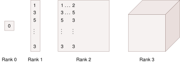](https://mlsysbook.ai/contents/core/frameworks/5a14326be5b802a50e34197aefbddc65a5cafdec.svg "Figure 7: Three-Dimensional Tensor: Higher-rank tensors extend the concepts of scalars, vectors, and matrices by arranging data in nested structures; this figure represents a three-dimensional tensor as a stack of matrices, enabling representation of complex, multi-dimensional data relationships. Tensors with rank greater than two are fundamental to representing data in areas like image processing and natural language processing, where data possesses inherent multi-dimensional structure.")
Figure 7: **Three-Dimensional Tensor**: Higher-rank tensors extend the concepts of scalars, vectors, and matrices by arranging data in nested structures; this figure represents a three-dimensional tensor as a stack of matrices, enabling representation of complex, multi-dimensional data relationships. Tensors with rank greater than two are fundamental to representing data in areas like image processing and natural language processing, where data possesses inherent multi-dimensional structure.
In practical applications, tensors naturally arise when dealing with complex data structures. As illustrated in [Figure 8](https://mlsysbook.ai/contents/core/frameworks/frameworks.html#fig-tensor-data-structure-b)
, image data exemplifies this concept particularly well. Color images comprise three channels, where each channel represents the intensity values of red, green, or blue as a distinct matrix. These channels combine to create the full colored image, forming a natural 3D tensor structure. When processing multiple images simultaneously, such as in batch operations, a fourth dimension can be added to create a 4D tensor, where each slice represents a complete three-channel image. This hierarchical organization demonstrates how tensors efficiently handle multidimensional data while maintaining clear structural relationships.
[](https://mlsysbook.ai/contents/core/frameworks/41ee5d842e2546a86bb5bd7ad4a245bd460a52e8.svg "Figure 8: Multidimensional Data Representation: Images naturally map to tensors with dimensions representing image height, width, and color channels, forming a three-dimensional array; stacking multiple images creates a fourth dimension for batch processing and efficient computation. credit: niklas lang https://towardsdatascience.com/what-are-tensors-in-machine-learning-5671814646ff.")
Figure 8: **Multidimensional Data Representation**: Images naturally map to tensors with dimensions representing image height, width, and color channels, forming a three-dimensional array; stacking multiple images creates a fourth dimension for batch processing and efficient computation. _credit: niklas lang [https://towardsdatascience.com/what-are-tensors-in-machine-learning-5671814646ff](https://towardsdatascience.com/what-are-tensors-in-machine-learning-5671814646ff)
_.
In machine learning frameworks, tensors take on additional properties beyond their mathematical definition to meet the demands of modern ML systems. While mathematical tensors provide a foundation as multi-dimensional arrays with transformation properties, machine learning introduces requirements for practical computation. These requirements shape how frameworks balance mathematical precision with computational performance.
Framework tensors combine numerical data arrays with computational metadata. The dimensional structure, or shape, ranges from simple vectors and matrices to higher-dimensional arrays that represent complex data like image batches or sequence models. This dimensional information plays a critical role in operation validation and optimization. Matrix multiplication operations, for example, depend on shape metadata to verify dimensional compatibility and determine optimal computation paths.
Memory layout implementation introduces distinct challenges in tensor design. While tensors provide an abstraction of multi-dimensional data, physical computer memory remains linear. Stride patterns address this disparity by creating mappings between multi-dimensional tensor indices and linear memory addresses. These patterns significantly impact computational performance by determining memory access patterns during tensor operations. [Figure 9](https://mlsysbook.ai/contents/core/frameworks/frameworks.html#fig-tensor-memory-layout)
demonstrates this concept using a 2×3 tensor, showing both row-major and column-major memory layouts with their corresponding stride calculations.
[](https://mlsysbook.ai/contents/core/frameworks/f78c7471ad0993e352f904eed876286c79655e7c.svg "Figure 9: Tensor Memory Layout: A 2×3 tensor can be stored in linear memory using either row-major (C-style) or column-major (Fortran-style) ordering. Strides define the number of elements to skip in each dimension when moving through memory, enabling frameworks to calculate memory addresses for tensor[i,j] as base_address + i×stride[0] + j×stride[1]. The choice of memory layout significantly impacts cache performance and computational efficiency.")
Figure 9: **Tensor Memory Layout**: A 2×3 tensor can be stored in linear memory using either row-major (C-style) or column-major (Fortran-style) ordering. Strides define the number of elements to skip in each dimension when moving through memory, enabling frameworks to calculate memory addresses for tensor\[i,j\] as base\_address + i×stride\[0\] + j×stride\[1\]. The choice of memory layout significantly impacts cache performance and computational efficiency.
Understanding these memory layout patterns is crucial for framework performance optimization. Row-major layout (used by NumPy, PyTorch) stores elements row by row, making row-wise operations more cache-friendly. Column-major layout (used by some BLAS libraries) stores elements column by column, optimizing column-wise access patterns. The stride values encode this layout information: in row-major layout for a 2×3 tensor, moving to the next row requires skipping 3 elements (stride\[0\]=3), while moving to the next column requires skipping 1 element (stride\[1\]=1).
Careful alignment of stride patterns with hardware memory hierarchies maximizes cache efficiency and memory throughput, with optimal layouts achieving 80-90% of theoretical memory bandwidth (typically 100-500GB/s on modern GPUs) compared to suboptimal patterns that may achieve only 20-30% utilization.
##### Type Systems and Precision
Tensor implementations use type systems to control numerical precision and memory consumption. The standard choice in machine learning has been 32-bit floating-point numbers (`float32`), offering a balance of precision and efficiency. Modern frameworks extend this with multiple numeric types for different needs. Integer types support indexing and embedding operations. Reduced-precision types like 16-bit floating-point numbers enable efficient mobile deployment. 8-bit integers allow fast inference on specialized hardware.
The choice of numeric type affects both model behavior and computational efficiency. Neural network training typically requires float32 precision to maintain stable gradient computations. Inference tasks can often use lower precision (`int8` or even `int4`), reducing memory usage and increasing processing speed. Mixed-precision training approaches combine these benefits by using float32 for critical accumulations while performing most computations at lower precision.
Type conversions between different numeric representations require careful management. Operating on tensors with different types demands explicit conversion rules to preserve numerical correctness. These conversions introduce computational costs and risk precision loss. Frameworks provide type casting capabilities but rely on developers to maintain numerical precision across operations.
##### Device and Memory Management
The rise of heterogeneous computing has transformed how machine learning frameworks manage tensor operations. Modern frameworks must seamlessly operate across CPUs, GPUs, TPUs, and various other accelerators, each offering different computational advantages and memory characteristics. This diversity creates a fundamental challenge: tensors must move efficiently between devices while maintaining computational coherency throughout the execution of machine learning workloads.
Device placement decisions significantly influence both computational performance and memory utilization. Moving tensors between devices introduces latency costs and consumes precious bandwidth on system interconnects. Keeping multiple copies of tensors across different devices can accelerate computation by reducing data movement, but this strategy increases overall memory consumption and requires careful management of consistency between copies. Frameworks must therefore implement sophisticated memory management systems that track tensor locations and orchestrate data movement while considering these tradeoffs.
These memory management systems maintain a dynamic view of available device memory and implement strategies for efficient data transfer. When operations require tensors that reside on different devices, the framework must either move data or redistribute computation. This decision process integrates deeply with the framework’s computational graph execution and operation scheduling. Memory pressure on individual devices, data transfer costs, and computational load all factor into placement decisions. Modern systems must optimize for data transfer rates that range from PCIe Gen4’s 32GB/s for CPU-GPU communication to NVLink’s 600GB/s for GPU-to-GPU transfers, with network interconnects typically providing 10-100Gbps for cross-node communication.
The interplay between device placement and memory management extends beyond simple data movement. Frameworks must anticipate future computational needs to prefetch data efficiently, manage memory fragmentation across devices, and handle cases where memory demands exceed device capabilities. This requires close coordination between the memory management system and the operation scheduler, especially in scenarios involving parallel computation across multiple devices or distributed training across machine boundaries. Efficient prefetching strategies can hide latency costs by overlapping data movement with computation, maintaining sustained throughput even when individual transfers operate at only 10-20% of peak bandwidth.
#### Domain-Specific Data Organizations
While tensors are the building blocks of machine learning frameworks, they are not the only structures required for effective system operation. Frameworks rely on a suite of specialized data structures tailored to address the distinct needs of data processing, model parameter management, and execution coordination. These structures ensure that the entire workflow, ranging from raw data ingestion to optimized execution on hardware, proceeds seamlessly and efficiently.
##### Dataset Structures
Dataset structures handle the critical task of transforming raw input data into a format suitable for machine learning computations. These structures seamlessly connect diverse data sources with the tensor abstractions required by models, automating the process of reading, parsing, and preprocessing data.
Dataset structures must support efficient memory usage while dealing with input data far larger than what can fit into memory at once. For example, when training on large image datasets, these structures load images from disk, decode them into tensor-compatible formats, and apply transformations like normalization or augmentation in real time. Frameworks implement mechanisms such as data streaming, caching, and shuffling to ensure a steady supply of preprocessed batches without bottlenecks.
The design of dataset structures directly impacts training performance. Poorly designed structures can create significant overhead, limiting data throughput to GPUs or other accelerators. In contrast, well-optimized dataset handling can leverage parallelism across CPU cores, disk I/O, and memory transfers to feed accelerators at full capacity. Modern training pipelines must sustain data loading rates of 1-10GB/s to match GPU computational throughput, requiring careful optimization of storage I/O patterns and preprocessing pipelines. Frameworks achieve this through techniques like parallel data loading, batch prefetching, and efficient data format selection (e.g., optimized formats can reduce loading overhead from 80% to under 10% of training time).
In large, multi-system distributed training scenarios, dataset structures also handle coordination between nodes, ensuring that each worker processes a distinct subset of data while maintaining consistency in operations like shuffling. This coordination prevents redundant computation and supports scalability across multiple devices and machines.
##### Parameter Structures
Parameter structures store the numerical values that define a machine learning model. These include the weights and biases of neural network layers, along with auxiliary data such as batch normalization statistics and optimizer state. Unlike datasets, which are transient, parameters persist throughout the lifecycle of model training and inference.
The design of parameter structures must balance efficient storage with rapid access during computation. For example, convolutional neural networks require parameters for filters, fully connected layers, and normalization layers, each with unique shapes and memory alignment requirements. Frameworks organize these parameters into compact representations that minimize memory consumption while enabling fast read and write operations.
A key challenge for parameter structures is managing memory efficiently across multiple devices ([Li et al. 2014](https://mlsysbook.ai/contents/core/frameworks/frameworks.html#ref-li2014communication)
). During distributed training, frameworks may replicate parameters across GPUs for parallel computation while keeping a synchronized master copy on the CPU. This strategy ensures consistency while reducing the latency of gradient updates. Parameter structures often leverage memory sharing techniques to minimize duplication, such as storing gradients and optimizer states in place to conserve memory. The communication costs for parameter synchronization can be substantial. Synchronizing a 7B parameter model across 8 GPUs requires transferring approximately 28GB of gradients (assuming FP32 precision), which at 25Gbps network speeds takes over 9 seconds without optimization, highlighting why frameworks implement gradient compression and efficient communication patterns like ring all-reduce.
Li, Mu, David G. Andersen, Jun Woo Park, Alexander J. Smola, Amr Ahmed, Vanja Josifovski, James Long, Eugene J. Shekita, and Bor-Yiing Su. 2014. “Communication Efficient Distributed Machine Learning with the Parameter Server.” In _Advances in Neural Information Processing Systems_, 27:19–27. [https://proceedings.neurips.cc/paper/2014/hash/a49e9411d64ff53eccfdd09ad10a15b3-Abstract.html](https://proceedings.neurips.cc/paper/2014/hash/a49e9411d64ff53eccfdd09ad10a15b3-Abstract.html)
.
Parameter structures must also adapt to various precision requirements. While training typically uses 32-bit floating-point precision for stability, reduced precision such as 16-bit floating-point or even 8-bit integers is increasingly used for inference and large-scale training. Frameworks implement type casting and mixed-precision management to enable these optimizations without compromising numerical accuracy.
##### Execution Structures
Execution structures coordinate how computations are performed on hardware, ensuring that operations execute efficiently while respecting device constraints. These structures work closely with computational graphs, determining how data flows through the system and how memory is allocated for intermediate results.
One of the primary roles of execution structures is memory management. During training or inference, intermediate computations such as activation maps or gradients can consume significant memory. Execution structures dynamically allocate and deallocate memory buffers to avoid fragmentation and maximize hardware utilization. For example, a deep neural network might reuse memory allocated for activation maps across layers, reducing the overall memory footprint.
These structures also handle operation scheduling, ensuring that computations are performed in the correct order and with optimal hardware utilization. On GPUs, for instance, execution structures can overlap computation and data transfer operations, hiding latency and improving throughput. When running on multiple devices, they synchronize dependent computations to maintain consistency without unnecessary delays.
Distributed training introduces additional complexity, as execution structures must manage data and computation across multiple nodes. This includes partitioning computational graphs, synchronizing gradients, and redistributing data as needed. Efficient execution structures minimize communication overhead, allowing distributed systems to scale linearly with additional hardware ([McMahan et al. 2017](https://mlsysbook.ai/contents/core/frameworks/frameworks.html#ref-mcmahan2023communicationefficient)
). [Figure 10](https://mlsysbook.ai/contents/core/frameworks/frameworks.html#fig-3d-parallelism)
shows how distributed training can be defined over a grid of accelerators to parallelize over multiple dimensions for faster throughput.
McMahan, Brendan, Eider Moore, Daniel Ramage, Seth Hampson, and Blaise Agüera y Arcas. 2017. “Communication-Efficient Learning of Deep Networks from Decentralized Data.” In _Proceedings of the 20th International Conference on Artificial Intelligence and Statistics, AISTATS 2017, 20-22 April 2017, Fort Lauderdale, FL, USA_, edited by Aarti Singh and Xiaojin (Jerry) Zhu, 54:1273–82. Proceedings of Machine Learning Research. PMLR. [http://proceedings.mlr.press/v54/mcmahan17a.html](http://proceedings.mlr.press/v54/mcmahan17a.html)
.
[](https://mlsysbook.ai/contents/core/frameworks/4c5f0685131801549fc8ff629df15c98025b87cc.svg "Figure 10: 3D Parallelism: Distributed training scales throughput by partitioning computation across multiple dimensions: data, pipeline stages, and model layers. This enables concurrent execution on a grid of accelerators. This approach minimizes communication overhead and maximizes hardware utilization by overlapping computation and communication across devices.")
Figure 10: **3D Parallelism**: Distributed training scales throughput by partitioning computation across multiple dimensions: data, pipeline stages, and model layers. This enables concurrent execution on a grid of accelerators. This approach minimizes communication overhead and maximizes hardware utilization by overlapping computation and communication across devices.
### Programming and Execution Models
The way developers _write_ code (the programming model) is closely tied to how frameworks _execute_ it (the execution model). Understanding this relationship reveals why different frameworks make different design trade-offs and how these decisions impact both development experience and system performance. This unified perspective shows how programming paradigms directly map to execution strategies, creating distinct framework characteristics that influence everything from debugging workflows to production optimization.
In machine learning frameworks, we can identify three primary paradigms that combine programming style with execution strategy: imperative programming with eager execution, symbolic programming with graph execution, and hybrid approaches with just-in-time (JIT) compilation. Each represents a different balance between developer flexibility and system optimization capabilities.
#### Declarative Model Definition and Optimized Execution
Symbolic programming involves constructing abstract representations of computations first and executing them later. This programming paradigm maps directly to graph execution, where the framework builds a complete computational graph before execution begins. The tight coupling between symbolic programming and graph execution enables powerful optimization opportunities while requiring developers to think in terms of complete computational workflows.
For instance, in symbolic programming, variables and operations are represented as symbols. These symbolic expressions are not evaluated until explicitly executed, allowing the framework to analyze and optimize the computation graph before running it.
Consider the symbolic programming example in [Listing 32](https://mlsysbook.ai/contents/core/frameworks/frameworks.html#lst-symbolic_example)
.
Listing 32: **Symbolic Computation (TensorFlow 1.x)**: Symbolic expressions are constructed without immediate evaluation, allowing for optimization before execution in machine learning workflows.
import tensorflow.compat.v1 as tf
tf.disable_v2_behavior()
# Expressions are constructed but not evaluated
weights = tf.Variable(tf.random.normal([784, 10]))
input_data = tf.placeholder(tf.float32, [None, 784])
output = tf.matmul(input_data, weights)
# Separate evaluation phase
with tf.Session() as sess:
sess.run(tf.global_variables_initializer())
result = sess.run(output, feed_dict={input_data: data})
This approach enables frameworks to apply global optimizations across the entire computation, making it efficient for deployment scenarios. Static graphs can be serialized and executed across different environments, enhancing portability. Predefined graphs also facilitate efficient parallel execution strategies. However, debugging can be challenging because errors often surface during execution rather than graph construction, and modifying a static graph dynamically is cumbersome.
#### Interactive Development with Immediate Execution
Imperative programming takes a more traditional approach, executing operations immediately as they are encountered. This programming paradigm maps directly to eager execution, where operations are computed as soon as they are called. The connection between imperative programming and eager execution creates dynamic computational graphs that evolve during execution, providing flexibility at the cost of optimization opportunities.
In this programming paradigm, computations are performed directly as the code executes, closely resembling the procedural style of most general-purpose programming languages. This is demonstrated in [Listing 33](https://mlsysbook.ai/contents/core/frameworks/frameworks.html#lst-imperative_example)
, where each operation is evaluated immediately.
Listing 33: **Imperative Execution**: Each operation is evaluated immediately as the code runs, highlighting how computations proceed step-by-step in dynamic computational graphs.
# Each expression evaluates immediately
weights = torch.randn(784, 10)
input = torch.randn(32, 784)
output = input @ weights # Computation occurs now
The immediate execution model is intuitive and aligns with common programming practices, making it easier to use. Errors can be detected and resolved immediately during execution, simplifying debugging. Dynamic graphs allow for adjustments on-the-fly, making them ideal for tasks requiring variable graph structures, such as reinforcement learning or sequence modeling. However, the creation of dynamic graphs at runtime can introduce computational overhead, and the framework’s ability to optimize the entire computation graph is limited due to the step-by-step execution process.
#### Performance versus Development Productivity Balance
The choice between symbolic and imperative programming models significantly influences how ML frameworks manage system-level features such as memory management and optimization strategies.
##### Performance Considerations
In symbolic programming, frameworks can analyze the entire computation graph upfront. This allows for efficient memory allocation strategies. For example, memory can be reused for intermediate results that are no longer needed during later stages of computation. This global view also enables advanced optimization techniques such as operation fusion, automatic differentiation, and hardware-specific kernel selection. These optimizations make symbolic programming highly effective for production environments where performance is critical.
In contrast, imperative programming makes memory management and optimization more challenging since decisions must be made at runtime. Each operation executes immediately, which prevents the framework from globally analyzing the computation. This trade-off, however, provides developers with greater flexibility and immediate feedback during development. Beyond system-level features, the choice of programming model also impacts the developer experience, particularly during model development and debugging.
##### Development and Debugging
Symbolic programming requires developers to conceptualize their models as complete computational graphs. This often involves extra steps to inspect intermediate values, as symbolic execution defers computation until explicitly invoked. For example, in TensorFlow 1.x, developers must use sessions and feed dictionaries to debug intermediate results, which can slow down the development process.
Imperative programming offers a more straightforward debugging experience. Operations execute immediately, allowing developers to inspect tensor values and shapes as the code runs. This immediate feedback simplifies experimentation and makes it easier to identify and fix issues in the model. As a result, imperative programming is well-suited for rapid prototyping and iterative model development.
##### Managing Trade-offs
The choice between symbolic and imperative programming models often depends on the specific needs of a project. Symbolic programming excels in scenarios where performance and optimization are critical, such as production deployments. In contrast, imperative programming provides the flexibility and ease of use necessary for research and development.
#### Adaptive Optimization Through Runtime Compilation
Modern frameworks have recognized that the choice between programming paradigms doesn’t need to be binary. Hybrid approaches combine the strengths of both paradigms through just-in-time (JIT) compilation, allowing developers to write code in an imperative style while achieving the performance benefits of graph execution.
JIT compilation represents the modern synthesis of programming and execution models. Developers write natural, imperative code that executes eagerly during development and debugging, but the framework can automatically convert frequently executed code paths into optimized static graphs for production deployment. This approach provides the best of both worlds: intuitive development experience with optimized execution performance.
Examples of this hybrid approach include TensorFlow’s `tf.function` decorator, which converts imperative Python functions into optimized graph execution, and PyTorch’s `torch.jit.script`, which compiles dynamic PyTorch models into static graphs. JAX takes this further with its `jit` transformation that provides automatic graph compilation and optimization.
These hybrid approaches demonstrate how modern frameworks have evolved beyond the traditional symbolic vs. imperative divide, recognizing that programming model and execution model can be decoupled to provide both developer productivity and system performance.
#### Execution Model Technical Implementation
Having established the three primary programming-execution paradigms, we can examine their implementation characteristics and performance implications. Each paradigm involves specific trade-offs in memory management, optimization capabilities, and development workflows that directly impact system performance and developer productivity.
#### Eager Execution
Eager execution is the most straightforward and intuitive execution paradigm. In this model, operations are executed immediately as they are called in the code. This approach closely mirrors the way traditional imperative programming languages work, making it familiar to many developers.
[Listing 34](https://mlsysbook.ai/contents/core/frameworks/frameworks.html#lst-eager_tf2)
demonstrates eager execution, where operations are evaluated immediately.
Listing 34: **Eager Execution**: Operations are evaluated immediately as they are called in the code, providing a more intuitive and flexible development experience.
import tensorflow as tf
x = tf.constant([[1.0, 2.0], [3.0, 4.0]])
y = tf.constant([[1, 2], [3, 4]])
z = tf.matmul(x, y)
print(z)
In this code snippet, each line is executed sequentially. When we create the tensors `x` and `y`, they are immediately instantiated in memory. The matrix multiplication `tf.matmul(x, y)` is computed right away, and the result is stored in `z`. When we print `z`, we see the output of the computation immediately.
Eager execution offers several advantages. It provides immediate feedback, allowing developers to inspect intermediate values easily. This makes debugging more straightforward and intuitive. It also allows for more dynamic and flexible code structures, as the computation graph can change with each execution.
However, eager execution has its trade-offs. Since operations are executed immediately, the framework has less opportunity to optimize the overall computation graph. This can lead to lower performance compared to more optimized execution paradigms, especially for complex models or when dealing with large datasets.
Eager execution is particularly well-suited for research, interactive development, and rapid prototyping. It allows data scientists and researchers to quickly iterate on their ideas and see results immediately. Many modern ML frameworks, including TensorFlow 2.x and PyTorch, use eager execution as their default mode due to its developer-friendly nature.
#### Graph Execution
Graph execution, also known as static graph execution, takes a different approach to computing operations in ML frameworks. In this paradigm, developers first define the entire computational graph, and then execute it as a separate step.
[Listing 35](https://mlsysbook.ai/contents/core/frameworks/frameworks.html#lst-tf1_graph_exec)
illustrates an example in TensorFlow 1.x style, which employs graph execution.
Listing 35: **Graph Execution (TensorFlow 1.x)**: Defines a computational graph and provides session-based evaluation to execute it, highlighting the separation between graph definition and execution.
import tensorflow.compat.v1 as tf
tf.disable_eager_execution()
# Define the graph
x = tf.placeholder(tf.float32, shape=(2, 2))
y = tf.placeholder(tf.float32, shape=(2, 2))
z = tf.matmul(x, y)
# Execute the graph
with tf.Session() as sess:
result = sess.run(
z,
feed_dict={x: [[1.0, 2.0], [3.0, 4.0]], y: [[1, 2], [3, 4]]},
)
print(result)
In this code snippet, we first define the structure of our computation. The `placeholder` operations create nodes in the graph for input data, while `tf.matmul` creates a node representing matrix multiplication. No actual computation occurs during this definition phase.
The execution of the graph happens when we create a session and call `sess.run()`. At this point, we provide the actual input data through the `feed_dict` parameter. The framework then has the complete graph and can perform optimizations before running the computation.
Graph execution offers several advantages. It allows the framework to see the entire computation ahead of time, enabling global optimizations that can improve performance, especially for complex models. Once defined, the graph can be easily saved and deployed across different environments, enhancing portability. It’s particularly efficient for scenarios where the same computation is repeated many times with different data inputs.
However, graph execution also has its trade-offs. It requires developers to think in terms of building a graph rather than writing sequential operations, which can be less intuitive. Debugging can be more challenging because errors often don’t appear until the graph is executed. Implementing dynamic computations can be more difficult with a static graph.
Graph execution is well-suited for production environments where performance and deployment consistency are crucial. It is commonly used in scenarios involving large-scale distributed training and when deploying models for predictions in high-throughput applications.
#### Dynamic Code Generation and Optimization
Just-In-Time compilation[24](https://mlsysbook.ai/contents/core/frameworks/frameworks.html#fn24)
is a middle ground between eager execution and graph execution. This paradigm aims to combine the flexibility of eager execution with the performance benefits of graph optimization.
24 **Just-In-Time (JIT) Compilation**: In ML frameworks, JIT compilation differs from traditional JIT by optimizing for tensor operations and hardware accelerators rather than general CPU instructions. ML JIT compilers like TensorFlow’s XLA and PyTorch’s TorchScript analyze computation patterns at runtime to generate optimized kernels for specific tensor shapes and device capabilities.
[Listing 36](https://mlsysbook.ai/contents/core/frameworks/frameworks.html#lst-jit_pytorch)
shows how scripted functions are compiled and reused in PyTorch.
Listing 36: **PyTorch JIT Compilation**: Compiles scripted functions for efficient reuse, illustrating how just-in-time compilation balances flexibility and performance in machine learning workflows.
import torch
@torch.jit.script
def compute(x, y):
return torch.matmul(x, y)
x = torch.randn(2, 2)
y = torch.randn(2, 2)
# First call compiles the function
result = compute(x, y)
print(result)
# Subsequent calls use the optimized version
result = compute(x, y)
print(result)
In this code snippet, we define a function `compute` and decorate it with `@torch.jit.script`. This decorator tells PyTorch to compile the function using its JIT compiler. The first time `compute` is called, PyTorch analyzes the function, optimizes it, and generates efficient machine code. This compilation process occurs just before the function is executed, hence the term “Just-In-Time”.
Subsequent calls to `compute` use the optimized version, potentially offering significant performance improvements, especially for complex operations or when called repeatedly.
JIT compilation provides a balance between development flexibility and runtime performance. It allows developers to write code in a natural, eager-style manner while still benefiting from many of the optimizations typically associated with graph execution.
This approach offers several advantages. It maintains the immediate feedback and intuitive debugging of eager execution, as most of the code still executes eagerly. At the same time, it can deliver performance improvements for critical parts of the computation. JIT compilation can also adapt to the specific data types and shapes being used, potentially resulting in more efficient code than static graph compilation.
However, JIT compilation also has some considerations. The first execution of a compiled function may be slower due to the overhead of the compilation process. Some complex Python constructs may not be easily JIT-compiled, requiring developers to be aware of what can be optimized effectively.
JIT compilation is particularly useful in scenarios where you need both the flexibility of eager execution for development and prototyping, and the performance benefits of compilation for production or large-scale training. It’s commonly used in research settings where rapid iteration is necessary but performance is still a concern.
Many modern ML frameworks incorporate JIT compilation to provide developers with a balance of ease-of-use and performance optimization, as shown in [Table 2](https://mlsysbook.ai/contents/core/frameworks/frameworks.html#tbl-mlfm-execmodes)
. This balance manifests across multiple dimensions, from the learning curve that gradually introduces optimization concepts to the runtime behavior that combines immediate feedback with performance enhancements. The table highlights how JIT compilation bridges the gap between eager execution’s programming simplicity and graph execution’s performance benefits, particularly in areas like memory usage and optimization scope.
Table 2: **Execution Model Trade-Offs**: Machine learning frameworks offer varying execution strategies (eager, graph, and JIT compilation) that balance programming flexibility with runtime performance. The table details how each approach differs in aspects like debugging ease, memory consumption, and the scope of optimization techniques applied during model training and inference.
| | | | |
| --- | --- | --- | --- |
| **Approach** | Computes each operation immediately when encountered | Builds entire computation plan first, then executes | Analyzes code at runtime, creates optimized version |
| **Memory Usage** | Holds intermediate results throughout computation | Optimizes memory by planning complete data flow | Adapts memory usage based on actual execution patterns |
| **Optimization Scope** | Limited to local operation patterns | Global optimization across entire computation chain | Combines runtime analysis with targeted optimizations |
| **Debugging Approach** | Examine values at any point during computation | Must set up specific monitoring points in graph | Initial runs show original behavior, then optimizes |
| **Speed vs Flexibility** | Prioritizes flexibility over speed | Prioritizes performance over flexibility | Balances flexibility and performance |
#### Distributed Execution
As machine learning models continue to grow in size and complexity, training them on a single device is often no longer feasible. Large models require significant computational power and memory, while massive datasets demand efficient processing across multiple machines. To address these challenges, modern AI frameworks provide built-in support for distributed execution, allowing computations to be split across multiple GPUs, TPUs, or distributed clusters. By abstracting the complexities of parallel execution, these frameworks enable practitioners to scale machine learning workloads efficiently while maintaining ease of use.
At the essence of distributed execution are two primary strategies: data parallelism[25](https://mlsysbook.ai/contents/core/frameworks/frameworks.html#fn25)
and model parallelism[26](https://mlsysbook.ai/contents/core/frameworks/frameworks.html#fn26)
. Data parallelism allows multiple devices to train the same model on different subsets of data, ensuring faster convergence without increasing memory requirements. Model parallelism, on the other hand, partitions the model itself across multiple devices, allowing the training of architectures too large to fit into a single device’s memory. While model parallelism comes in several variations explored in detail in **[Chapter 8: AI Training](https://mlsysbook.ai/contents/core/training/training.html#sec-ai-training)
**, both techniques are essential for training modern machine learning models efficiently. These distributed execution strategies become increasingly important as models scale to the sizes discussed in **[Chapter 9: Efficient AI](https://mlsysbook.ai/contents/core/efficient_ai/efficient_ai.html#sec-efficient-ai)
**, and their implementation requires the hardware acceleration techniques covered in **[Chapter 11: AI Acceleration](https://mlsysbook.ai/contents/core/hw_acceleration/hw_acceleration.html#sec-ai-acceleration)
**.
25 **Data Parallelism**: A distributed training strategy where identical model copies process different data subsets in parallel, then synchronize gradients. Enables near-linear speedup with additional devices but requires models that fit in single-device memory, making it ideal for training on datasets with billions of samples.
26 **Model Parallelism**: A strategy for training models too large for single devices by partitioning the model architecture across multiple processors. Essential for models like GPT-3 (175B parameters) that exceed GPU memory limits, though it requires careful optimization to minimize communication overhead between model partitions.
##### Data Parallelism
Data parallelism is the most widely used approach for distributed training, enabling machine learning models to scale across multiple devices while maintaining efficiency. In this method, each computing device holds an identical copy of the model but processes a unique subset of the training data, as illustrated in [Figure 11](https://mlsysbook.ai/contents/core/frameworks/frameworks.html#fig-data-fm-parallelism)
. Once the computations are complete, the gradients computed on each device are synchronized before updating the model parameters, ensuring consistency across all copies. This approach allows models to learn from larger datasets in parallel without increasing memory requirements per device.
[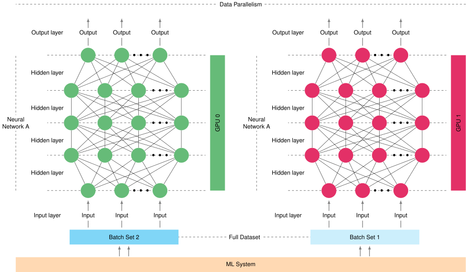](https://mlsysbook.ai/contents/core/frameworks/f35f3f52bd5ee07e1e3259618b5da5784969adae.svg "Figure 11: ")
Figure 11
Data parallelism distributes training data across multiple devices while maintaining identical model copies on each device, enabling significant speedup for large datasets. AI frameworks provide built-in mechanisms to manage the key challenges of data parallel execution, including data distribution, gradient synchronization, and performance optimization. In PyTorch, the `DistributedDataParallel (DDP)` module automates these tasks, ensuring efficient training across multiple GPUs or nodes. TensorFlow offers `tf.distribute.MirroredStrategy`, which enables seamless gradient synchronization for multi-GPU training. Similarly, JAX’s `pmap()` function facilitates parallel execution across multiple accelerators, optimizing inter-device communication to reduce overhead. These frameworks abstract the complexity of gradient aggregation, which can require 10-100Gbps network bandwidth for large models. For instance, synchronizing gradients for a 175B parameter model across 1024 GPUs requires communicating approximately 700GB of data per training step (FP32 precision), necessitating sophisticated algorithms to achieve near-linear scaling efficiency.
By handling synchronization and communication automatically, these frameworks make distributed training accessible to a wide range of users, from researchers exploring novel architectures to engineers deploying large-scale AI systems. The implementation details vary, but the fundamental goal remains the same: enabling efficient multi-device training without requiring users to manually manage low-level parallelization.
##### Model Parallelism
While data parallelism is effective for many machine learning workloads, some models are too large to fit within the memory of a single device. Model parallelism addresses this limitation by partitioning the model itself across multiple devices, allowing each to process a different portion of the computation. Unlike data parallelism, where the entire model is replicated on each device, model parallelism divides layers, tensors, or specific operations among available hardware resources, as shown in [Figure 12](https://mlsysbook.ai/contents/core/frameworks/frameworks.html#fig-fm-model-parallelism)
. This approach enables training of large-scale models that would otherwise be constrained by single-device memory limits.
[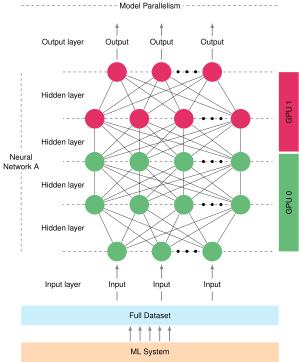](https://mlsysbook.ai/contents/core/frameworks/9cedc1b9fd9356814150321f0584b322a99f62bd.svg "Figure 12: ")
Figure 12
Model parallelism addresses memory constraints by distributing different parts of the model across multiple devices, enabling training of models too large for a single device. AI frameworks provide structured APIs to simplify model parallel execution, abstracting away much of the complexity associated with workload distribution and communication. PyTorch supports pipeline parallelism through `torch.distributed.pipeline.sync`, enabling different GPUs to process sequential layers of a model while maintaining efficient execution flow. TensorFlow’s `TPUStrategy` allows for automatic partitioning of large models across TPU cores, optimizing execution for high-speed interconnects. Frameworks like DeepSpeed and Megatron-LM extend PyTorch by implementing advanced model sharding techniques, including tensor parallelism, which splits model weights across multiple devices to reduce memory overhead. These techniques must manage substantial communication overhead. Tensor parallelism typically requires 100-400GB/s inter-device bandwidth to maintain efficiency, while pipeline parallelism can operate effectively with lower bandwidth (10-50Gbps) due to less frequent but larger activation transfers between pipeline stages.
There are multiple variations of model parallelism, each suited to different architectures and hardware configurations. Multiple parallelism strategies exist for different architectures and hardware configurations. The specific trade-offs and applications of these techniques are explored in **[Chapter 8: AI Training](https://mlsysbook.ai/contents/core/training/training.html#sec-ai-training)
** for distributed training strategies, and [Figure 13](https://mlsysbook.ai/contents/core/frameworks/frameworks.html#fig-tensor-vs-pipeline-parallelism)
shows some initial intuition in comparing parallelism strategies. Regardless of the exact approach, AI frameworks play an important role in managing workload partitioning, scheduling computations efficiently, and minimizing communication overhead, ensuring that even the largest models can be trained at scale.
[](https://mlsysbook.ai/contents/core/frameworks/27fdbfcc3a5ec88cce2f3cb453a3ef4be91985cb.svg "Figure 13: Parallelism Strategies: Tensor parallelism shards individual layers across multiple devices, reducing per-device memory requirements, while pipeline parallelism distributes consecutive layers to different devices, increasing throughput by overlapping computation and communication. This figure contrasts these approaches, highlighting how tensor parallelism replicates layer parameters across devices and pipeline parallelism partitions the model’s computational graph.")
Figure 13: **Parallelism Strategies**: Tensor parallelism shards individual layers across multiple devices, reducing per-device memory requirements, while pipeline parallelism distributes consecutive layers to different devices, increasing throughput by overlapping computation and communication. This figure contrasts these approaches, highlighting how tensor parallelism replicates layer parameters across devices and pipeline parallelism partitions the model’s computational graph.
### Core Operations
Machine learning frameworks employ a three-layer operational hierarchy that transforms high-level model descriptions into efficient hardware computations. [Figure 14](https://mlsysbook.ai/contents/core/frameworks/frameworks.html#fig-mlfm-core-ops)
illustrates how hardware abstraction operations manage computing platform complexity, basic numerical operations implement mathematical computations, and system-level operations coordinate resources and execution.
[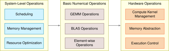](https://mlsysbook.ai/contents/core/frameworks/70f03560d31cd9df27454d9b2068f101cacd6b97.svg "Figure 14: Framework Operational Hierarchy: Machine learning frameworks abstract hardware complexities through layered operations (scheduling, memory management, and resource optimization), enabling efficient execution of mathematical models on diverse computing platforms. This hierarchical structure transforms high-level model descriptions into practical implementations by coordinating resources and managing computations.")
Figure 14: **Framework Operational Hierarchy**: Machine learning frameworks abstract hardware complexities through layered operations (scheduling, memory management, and resource optimization), enabling efficient execution of mathematical models on diverse computing platforms. This hierarchical structure transforms high-level model descriptions into practical implementations by coordinating resources and managing computations.
#### Hardware Abstraction Operations
Hardware abstraction operations form the foundation layer, isolating higher levels from platform-specific details while maintaining computational efficiency. This layer handles compute kernel management, memory system abstraction, and execution control across diverse computing platforms.
##### Compute Kernel Management
Compute kernel management involves selecting and dispatching optimal implementations of mathematical operations for different hardware architectures. This requires maintaining multiple implementations of core operations and sophisticated dispatch logic. For example, a matrix multiplication operation might be implemented using AVX-512 vector instructions on modern CPUs, [cuBLAS](https://developer.nvidia.com/cublas)
on NVIDIA GPUs, or specialized tensor processing instructions on AI accelerators. The kernel manager must consider input sizes, data layout, and hardware capabilities when selecting implementations. It must also handle fallback paths for when specialized implementations are unavailable or unsuitable.
##### Memory System Abstraction
Memory system abstractions manage data movement through complex memory hierarchies. These abstractions must handle various memory types (registered, pinned, unified) and their specific access patterns. Data layouts often require transformation between hardware-preferred formats - for instance, between row-major and column-major matrix layouts, or between interleaved and planar image formats. The memory system must also manage alignment requirements, which can vary from 4-byte alignment on CPUs to 128-byte alignment on some accelerators. Additionally, it handles cache coherency issues when multiple execution units access the same data.
##### Execution Control
Execution control operations coordinate computation across multiple execution units and memory spaces. This includes managing execution queues, handling event dependencies, and controlling asynchronous operations. Modern hardware often supports multiple execution streams that can operate concurrently. For example, independent GPU streams or CPU thread pools. The execution controller must manage these streams, handle synchronization points, and ensure correct ordering of dependent operations. It must also provide error handling and recovery mechanisms for hardware-specific failures.
#### Basic Numerical Operations
Building upon the hardware abstraction layer established above, frameworks implement fundamental numerical operations balancing mathematical precision with computational efficiency. General Matrix Multiply (GEMM) operations dominate ML computational costs, following the pattern C = \\(\\alpha\\)AB + \\(\\beta\\)C, where A, B, and C are matrices, and \\(\\alpha\\) and \\(\\beta\\) are scaling factors.
The implementation of GEMM operations requires sophisticated optimization techniques. These include blocking for cache efficiency, where matrices are divided into smaller tiles that fit in cache memory; loop unrolling to increase instruction-level parallelism; and specialized implementations for different matrix shapes and sparsity patterns. For example, fully-connected neural network layers typically use regular dense GEMM operations, while convolutional layers often employ specialized GEMM variants that exploit input locality patterns.
Beyond GEMM, frameworks must efficiently implement BLAS operations such as vector addition (AXPY), matrix-vector multiplication (GEMV), and various reduction operations. These operations require different optimization strategies. AXPY operations are typically memory-bandwidth limited, while GEMV operations must balance memory access patterns with computational efficiency.
Element-wise operations form another critical category, including both basic arithmetic operations (addition, multiplication) and transcendental functions (exponential, logarithm, trigonometric functions). While conceptually simpler than GEMM, these operations present significant optimization opportunities through vectorization and operation fusion. For example, multiple element-wise operations can often be fused into a single kernel to reduce memory bandwidth requirements. The efficiency of these operations becomes particularly important in neural network activation functions and normalization layers, where they process large volumes of data.
Modern frameworks must also handle operations with varying numerical precision requirements. For example, training often requires 32-bit floating-point precision for numerical stability, while inference can often use reduced precision formats like 16-bit floating-point or even 8-bit integers. Frameworks must therefore provide efficient implementations across multiple numerical formats while maintaining acceptable accuracy.
#### System-Level Operations
System-level operations build upon the computational graph foundation and hardware abstractions to manage overall computation flow and resource utilization through operation scheduling, memory management, and resource optimization.
Operation scheduling leverages the computational graph structure discussed earlier to determine execution ordering. Using the static or dynamic graph representation, the scheduler must identify parallelization opportunities while respecting dependencies. The implementation challenges differ between static graphs, where the entire dependency structure is known in advance, and dynamic graphs, where dependencies emerge during execution. The scheduler must also handle advanced execution patterns like conditional operations and loops that create dynamic control flow within the graph structure.
Memory management implements sophisticated strategies for allocating and deallocating memory resources across the computational graph. Different data types require different management strategies. Model parameters typically persist throughout execution and may require specific memory types for efficient access. Intermediate results have bounded lifetimes defined by the operation graph. For example, activation values are needed only during the backward pass. The memory manager employs techniques like reference counting for automatic cleanup, memory pooling to reduce allocation overhead, and workspace management for temporary buffers. It must also handle memory fragmentation, particularly in long-running training sessions where allocation patterns can change over time.
Resource optimization integrates scheduling and memory decisions to maximize performance within system constraints. A key optimization is gradient checkpointing, where some intermediate results are discarded and recomputed rather than stored, trading computation time for memory savings. The optimizer must also manage concurrent execution streams, balancing load across available compute units while respecting dependencies. For operations with multiple possible implementations, it selects between alternatives based on runtime conditions - for instance, choosing between matrix multiplication algorithms based on matrix shapes and system load.
Together, these operational layers build upon the computational graph foundation established in [Section 1.3.1](https://mlsysbook.ai/contents/core/frameworks/frameworks.html#sec-ai-frameworks-computational-graphs-f0ff)
to execute machine learning workloads efficiently while abstracting implementation complexity from model developers. The interaction between these layers determines overall system performance and sets the foundation for advanced optimization techniques discussed in **[Chapter 10: Model Optimizations](https://mlsysbook.ai/contents/core/optimizations/optimizations.html#sec-model-optimizations)
** and **[Chapter 11: AI Acceleration](https://mlsysbook.ai/contents/core/hw_acceleration/hw_acceleration.html#sec-ai-acceleration)
**.
Having explored the fundamental concepts enabling framework functionality, we now examine how these concepts are packaged into practical development interfaces. Framework architecture defines how the underlying computational machinery is exposed to developers through APIs and abstractions that balance usability with performance.
**Self-Check: Question 1.3**
1. Which layer in a machine learning framework is responsible for managing numerical data and optimizing memory usage?
1. Data Handling
2. Developer Interface
3. Fundamentals
4. Execution and Abstraction
2. Explain how the Developer Interface layer influences the behavior of machine learning models in a framework.
3. Order the following layers of a machine learning framework from top to bottom in terms of their position in the architecture: (1) Execution and Abstraction, (2) Fundamentals, (3) Developer Interface, (4) Data Handling.
[See Answers →](https://mlsysbook.ai/contents/core/frameworks/frameworks.html#quiz-answer-sec-ai-frameworks-fundamental-concepts-a6cf)
Framework Architecture
----------------------
While the fundamental concepts provide the computational foundation, practical framework usage depends on well-designed architectural interfaces that make this power accessible to developers. Framework architecture organizes the capabilities we have discussed (computational graphs, execution models, and optimized operations) into structured layers that serve different aspects of the development workflow. Understanding these architectural choices helps developers leverage frameworks effectively and select appropriate tools for their specific requirements.
### APIs and Abstractions
The API layer of machine learning frameworks provides the primary interface through which developers interact with the framework’s capabilities. This layer must balance multiple competing demands: it must be intuitive enough for rapid development, flexible enough to support diverse use cases, and efficient enough to enable high-performance implementations.
Modern framework APIs implement multiple abstraction levels to address competing requirements. Low-level APIs provide direct access to tensor operations and computational graph construction, exposing the fundamental operations discussed previously for fine-grained control over computation, as illustrated in [Listing 37](https://mlsysbook.ai/contents/core/frameworks/frameworks.html#lst-low_level_api)
.
Listing 37: **Manual Tensor Operations**: To perform custom computations using pytorch’s low-level API, highlighting the flexibility for defining complex transformations.
import torch
# Manual tensor operations
x = torch.randn(2, 3)
w = torch.randn(3, 4)
b = torch.randn(4)
y = torch.matmul(x, w) + b
# Manual gradient computation
y.backward(torch.ones_like(y))
Building on this low-level foundation, frameworks provide higher-level APIs that package common patterns into reusable components. Neural network layers exemplify this approach, where pre-built layer abstractions handle implementation details rather than requiring manual tensor operations, as shown in [Listing 38](https://mlsysbook.ai/contents/core/frameworks/frameworks.html#lst-mid_level_api)
.
Listing 38: **Mid-Level Abstraction**: Neural networks are constructed using layers like convolutions and fully connected layers, showcasing how high-level models build upon basic tensor operations for efficient implementation.
import torch.nn as nn
class SimpleNet(nn.Module):
def __init__(self):
super().__init__()
self.conv = nn.Conv2d(3, 64, kernel_size=3)
self.fc = nn.Linear(64, 10)
def forward(self, x):
x = self.conv(x)
x = torch.relu(x)
x = self.fc(x)
return x
This layered approach culminates in comprehensive workflow automation. At the highest level ([Listing 39](https://mlsysbook.ai/contents/core/frameworks/frameworks.html#lst-high_level_api)
), frameworks often provide model-level abstractions that automate common workflows. For example, the Keras API provides a highly abstract interface that hides most implementation details:
Listing 39: **High-level model definition**: Defines a convolutional neural network architecture using Keras, showcasing layer stacking for feature extraction and classification. Training workflow: Automates the training process by compiling the model with an optimizer and loss function, then fitting it to data over multiple epochs.
from tensorflow import keras
model = keras.Sequential(
[\
keras.layers.Conv2D(\
64, 3, activation="relu", input_shape=(32, 32, 3)\
),\
keras.layers.Flatten(),\
keras.layers.Dense(10),\
]
)
# Automated training workflow
model.compile(
optimizer="adam", loss="sparse_categorical_crossentropy"
)
model.fit(train_data, train_labels, epochs=10)
The organization of these API layers reflects fundamental trade-offs in framework design. Lower-level APIs provide maximum flexibility but require more expertise to use effectively. Higher-level APIs improve developer productivity but may constrain implementation choices. Framework APIs must therefore provide clear paths between abstraction levels, allowing developers to mix different levels of abstraction as needed for their specific use cases.
These carefully designed API layers provide the interface between developers and framework capabilities, but they represent only one component of the complete development experience. While APIs define how developers interact with frameworks, the complete development experience depends on the broader ecosystem of tools, libraries, and resources that surround the core framework. This ecosystem extends framework capabilities beyond basic model implementation to encompass the entire machine learning lifecycle.
**Self-Check: Question 1.4**
1. Which of the following best describes the role of low-level APIs in machine learning frameworks?
1. They provide direct access to tensor operations and computational graph construction.
2. They automate the entire training workflow.
3. They offer pre-built layer abstractions for common patterns.
4. They abstract away all implementation details for ease of use.
2. Explain how high-level APIs in machine learning frameworks improve developer productivity.
3. The API layer of machine learning frameworks must balance being intuitive, flexible, and \_\_\_\_ to enable high-performance implementations.
4. Order the following API layers from lowest to highest level of abstraction: (1) High-level model definition, (2) Low-level tensor operations, (3) Mid-level neural network layers.
5. In a production system, why might a developer choose to use a low-level API instead of a high-level API?
[See Answers →](https://mlsysbook.ai/contents/core/frameworks/frameworks.html#quiz-answer-sec-ai-frameworks-framework-architecture-0982)
Framework Ecosystem
-------------------
Machine learning frameworks organize their fundamental capabilities into distinct components that work together to provide a complete development and deployment environment. These components create layers of abstraction that make frameworks both usable for high-level model development and efficient for low-level execution. Understanding how these components interact helps developers choose and use frameworks effectively, particularly as they support the complete ML lifecycle from data preprocessing **[Chapter 6: Data Engineering](https://mlsysbook.ai/contents/core/data_engineering/data_engineering.html#sec-data-engineering)
** through training **[Chapter 8: AI Training](https://mlsysbook.ai/contents/core/training/training.html#sec-ai-training)
** to deployment **[Chapter 13: ML Operations](https://mlsysbook.ai/contents/core/ops/ops.html#sec-ml-operations)
**. This ecosystem approach bridges the theoretical foundations presented in **[Chapter 3: Deep Learning Primer](https://mlsysbook.ai/contents/core/dl_primer/dl_primer.html#sec-dl-primer)
** with the practical requirements of production ML systems described in **[Chapter 2: ML Systems](https://mlsysbook.ai/contents/core/ml_systems/ml_systems.html#sec-ml-systems)
**.
### Core Libraries
At the heart of every machine learning framework lies a set of core libraries, forming the foundation upon which all other components are built. These libraries provide the essential building blocks for machine learning operations, implementing fundamental tensor operations that serve as the backbone of numerical computations. Heavily optimized for performance, these operations often leverage low-level programming languages and hardware-specific optimizations to ensure efficient execution of tasks like matrix multiplication, a cornerstone of neural network computations.
These computational primitives support more sophisticated capabilities. Alongside these basic operations, core libraries implement automatic differentiation capabilities, enabling the efficient computation of gradients for complex functions. This feature is crucial for the gradient-based training that powers most neural network optimization. The implementation often involves intricate graph manipulation and symbolic computation techniques, abstracting away the complexities of gradient calculation from the end-user.
These foundational capabilities enable higher-level abstractions that accelerate development. Building upon these fundamental operations, core libraries typically provide pre-implemented neural network layers such as various neural network layer types. These ready-to-use components save developers from reinventing the wheel for common model architectures, allowing them to focus on higher-level model design rather than low-level implementation details. Similarly, optimization algorithms are provided out-of-the-box, further streamlining the model development process.
The integration of these components creates a cohesive development environment. A simplified example of how these components might be used in practice is shown in [Listing 40](https://mlsysbook.ai/contents/core/frameworks/frameworks.html#lst-integrated_example)
.
Listing 40: **Training Pipeline**: Machine learning workflows partition datasets into training, validation, and test sets to ensure robust model development and unbiased evaluation.
import torch
import torch.nn as nn
# Create a simple neural network
model = nn.Sequential(nn.Linear(10, 20), nn.ReLU(), nn.Linear(20, 1))
# Define loss function and optimizer
loss_fn = nn.MSELoss()
optimizer = torch.optim.Adam(model.parameters(), lr=0.01)
# Forward pass, compute loss, and backward pass
x = torch.randn(32, 10)
y = torch.randn(32, 1)
y_pred = model(x)
loss = loss_fn(y_pred, y)
loss.backward()
optimizer.step()
This example demonstrates how core libraries provide high-level abstractions for model creation, loss computation, and optimization, while handling low-level details internally. The seamless integration of these components exemplifies how core libraries create the foundation for the broader framework ecosystem.
### Extensions and Plugins
While core libraries offer essential functionality, the true power of modern machine learning frameworks often lies in their extensibility. Extensions and plugins expand the capabilities of frameworks, allowing them to address specialized needs and leverage recent research advances. Domain-specific libraries, for instance, cater to particular areas like computer vision or natural language processing, providing pre-trained models, specialized data augmentation techniques, and task-specific layers.
Beyond domain specialization, performance optimization drives another crucial category of extensions. Hardware acceleration plugins play an important role in performance optimization as it enables frameworks to take advantage of specialized hardware like GPUs or TPUs. These plugins dramatically speed up computations and allow seamless switching between different hardware backends, a key feature for scalability and flexibility in modern machine learning workflows.
The increasing scale of modern machine learning creates additional extension needs. As models and datasets grow in size and complexity, distributed computing extensions also become important. These tools enable training across multiple devices or machines, handling complex tasks like data parallelism, model parallelism, and synchronization between compute nodes. This capability is essential for researchers and companies tackling large-scale machine learning problems.
To support the research and development process, complementing these computational tools are visualization and experiment tracking extensions. Visualization tools provide invaluable insights into the training process and model behavior, displaying real-time metrics and even offering interactive debugging capabilities. Experiment tracking extensions help manage the complexity of machine learning research, allowing systematic logging and comparison of different model configurations and hyperparameters.
### Integrated Development and Debugging Environment
Beyond the core framework and its extensions, the ecosystem of development tools surrounding a machine learning framework further enhances its effectiveness and adoption. Interactive development environments, such as Jupyter notebooks, have become nearly ubiquitous in machine learning workflows, allowing for rapid prototyping and seamless integration of code, documentation, and outputs. Many frameworks provide custom extensions for these environments to enhance the development experience.
The complexity of machine learning systems requires specialized development support. Debugging and profiling tools address the unique challenges presented by machine learning models. Specialized debuggers allow developers to inspect the internal state of models during training and inference, while profiling tools identify bottlenecks in model execution, guiding optimization efforts. These tools are essential for developing efficient and reliable machine learning systems.
As projects grow in complexity, version control integration becomes increasingly important. Tools that allow versioning of not just code, but also model weights, hyperparameters, and training data, help manage the iterative nature of model development. This comprehensive versioning approach ensures reproducibility and facilitates collaboration in large-scale machine learning projects.
Finally, deployment utilities streamline the transition between development and production environments. These tools handle tasks like model compression, conversion to deployment-friendly formats, and integration with serving infrastructure, streamlining the process of moving models from experimental settings to real-world applications.
**Self-Check: Question 1.5**
1. Which component of a machine learning framework is primarily responsible for implementing fundamental tensor operations?
1. Development tools
2. Extensions and plugins
3. Core libraries
4. Deployment utilities
2. Explain how extensions and plugins enhance the capabilities of machine learning frameworks.
3. What is a key advantage of using hardware acceleration plugins in machine learning frameworks?
1. Improved user interface design
2. Enhanced visualization capabilities
3. Simplified data preprocessing
4. Faster computation on specialized hardware
4. How do development tools within a machine learning framework ecosystem support efficient model development?
[See Answers →](https://mlsysbook.ai/contents/core/frameworks/frameworks.html#quiz-answer-sec-ai-frameworks-framework-ecosystem-4f2e)
System Integration
------------------
Moving from development environments to production deployment requires careful consideration of system integration challenges. System integration is about implementing machine learning frameworks in real-world environments. This section explores how ML frameworks integrate with broader software and hardware ecosystems, addressing the challenges and considerations at each level of the integration process.
### Hardware Integration
Effective hardware integration is crucial for optimizing the performance of machine learning models. Modern ML frameworks must adapt to a diverse range of computing environments, from high-performance GPU clusters to resource-constrained edge devices.
This adaptation begins with accelerated computing platforms. For GPU acceleration, frameworks like TensorFlow and PyTorch provide robust support, allowing seamless utilization of NVIDIA’s CUDA platform. This integration enables significant speedups in both training and inference tasks. Similarly, support for Google’s TPUs in TensorFlow allows for even further acceleration of specific workloads.
In distributed computing scenarios, frameworks must efficiently manage multi-device and multi-node setups through sophisticated coordination abstractions. Data parallelism replicates the same model across devices and requires all-reduce communication patterns. Frameworks implement ring all-reduce algorithms that achieve O(N) communication complexity with optimal bandwidth utilization for large gradients, typically achieving 85-95% of theoretical network bandwidth on high-speed interconnects like InfiniBand (100-400Gbps). Model parallelism distributes different model partitions across hardware units, necessitating point-to-point communication between partitions and careful synchronization of forward and backward passes, with communication overhead often consuming 20-40% of total training time when network bandwidth falls below 25Gbps per node. At scale, failure becomes inevitable: Google reports TPU pod training jobs experience failures every few hours due to memory errors, hardware failures, and network partitions. Modern frameworks address this through elastic training capabilities that adapt to changing cluster sizes dynamically and checkpointing strategies that save model state every N iterations. Frameworks like Horovod[27](https://mlsysbook.ai/contents/core/frameworks/frameworks.html#fn27)
and specialized systems like DeepSpeed have emerged to abstract these distributed training complexities across different backend frameworks, optimizing communication patterns to sustain training throughput even when aggregate network bandwidth utilization exceeds 80% of available capacity.
27 **Horovod**: Uber’s distributed deep learning training framework that provides a single API for data-parallel training across TensorFlow, Keras, PyTorch, and MXNet. Implements ring-allreduce algorithms achieving 85-95% of theoretical network bandwidth utilization on high-speed interconnects.
For edge deployment, frameworks are increasingly offering lightweight versions optimized for mobile and IoT devices. TensorFlow Lite and PyTorch Mobile, for instance, provide tools for model compression and optimization, ensuring efficient execution on devices with limited computational resources and power constraints.
### Framework Infrastructure Dependencies
Integrating ML frameworks into existing software stacks presents unique challenges and opportunities. A key consideration is how the ML system interfaces with data processing pipelines. Frameworks often provide connectors to popular big data tools like Apache Spark or Apache Beam, allowing seamless data flow between data processing systems and ML training environments.
Containerization technologies like Docker have become essential in ML workflows, ensuring consistency between development and production environments. Kubernetes has emerged as a popular choice for orchestrating containerized ML workloads, providing scalability and manageability for complex deployments.
ML frameworks must also interface with other enterprise systems such as databases, message queues, and web services. For instance, TensorFlow Serving provides a flexible, high-performance serving system for machine learning models, which can be easily integrated into existing microservices architectures.
### Production Environment Integration Requirements
Deploying ML models to production environments involves several critical considerations. Model serving strategies must balance performance, scalability, and resource efficiency. Approaches range from batch prediction for large-scale offline processing to real-time serving for interactive applications.
Scaling ML systems to meet production demands often involves techniques like horizontal scaling of inference servers, caching of frequent predictions, and load balancing across multiple model versions. Frameworks like TensorFlow Serving and TorchServe provide built-in solutions for many of these scaling challenges.
Monitoring and logging are crucial for maintaining ML systems in production. This includes tracking model performance metrics, detecting concept drift, and logging prediction inputs and outputs for auditing purposes. Tools like Prometheus and Grafana are often integrated with ML serving systems to provide comprehensive monitoring solutions.
### End-to-End Machine Learning Pipeline Management
Managing end-to-end ML pipelines requires orchestrating multiple stages, from data preparation and model training to deployment and monitoring. MLOps practices have emerged to address these challenges, bringing DevOps principles to machine learning workflows.
Continuous Integration and Continuous Deployment (CI/CD) practices are being adapted for ML workflows. This involves automating model testing, validation, and deployment processes. Tools like Jenkins or GitLab CI can be extended with ML-specific stages to create robust CI/CD pipelines for machine learning projects.
Automated model retraining and updating is another critical aspect of ML workflow orchestration. This involves setting up systems to automatically retrain models on new data, evaluate their performance, and seamlessly update production models when certain criteria are met. Frameworks like Kubeflow provide end-to-end ML pipelines that can automate many of these processes. [Figure 15](https://mlsysbook.ai/contents/core/frameworks/frameworks.html#fig-workflow-orchestration)
shows an example orchestration flow, where a user submits DAGs, or directed acyclic graphs of workloads to process and train to be executed.
Version control for ML assets, including data, model architectures, and hyperparameters, is essential for reproducibility and collaboration. Tools like DVC (Data Version Control) and MLflow have emerged to address these ML-specific version control needs.
[](https://mlsysbook.ai/contents/core/frameworks/d321bea9bf11f492ca58987e8844cf6e67bd2722.svg "Figure 15: Workflow Orchestration: Data engineering and machine learning pipelines benefit from orchestration tools like Airflow, which automate task scheduling, distributed execution, and result monitoring for repeatable and scalable model training and deployment. Directed acyclic graphs (DAGs) define these workflows, enabling complex sequences of operations to be managed efficiently as part of a CI/CD system.")
Figure 15: **Workflow Orchestration**: Data engineering and machine learning pipelines benefit from orchestration tools like Airflow, which automate task scheduling, distributed execution, and result monitoring for repeatable and scalable model training and deployment. Directed acyclic graphs (DAGs) define these workflows, enabling complex sequences of operations to be managed efficiently as part of a CI/CD system.
**Self-Check: Question 1.6**
1. Which of the following is a key challenge when integrating ML frameworks with hardware systems?
1. Ensuring compatibility with all programming languages
2. Providing a user-friendly graphical interface
3. Optimizing performance across diverse computing environments
4. Supporting only CPU-based computations
2. True or False: TensorFlow and PyTorch provide support for GPU acceleration through NVIDIA’s CUDA platform.
3. Explain how distributed computing scenarios are managed by ML frameworks to optimize training performance.
4. Frameworks like TensorFlow Lite and PyTorch Mobile are designed for \_\_\_\_\_\_\_\_ deployment, optimizing models for devices with limited computational resources.
5. Order the following steps in a typical ML deployment process: (1) Model training, (2) Model serving, (3) Monitoring and logging, (4) Hardware integration.
[See Answers →](https://mlsysbook.ai/contents/core/frameworks/frameworks.html#quiz-answer-sec-ai-frameworks-system-integration-624f)
Major Framework Platform Analysis
---------------------------------
Having explored the fundamental concepts, architecture, and ecosystem components that define modern frameworks, we now examine how these principles manifest in real-world implementations. Machine learning frameworks exhibit considerable architectural complexity. Over the years, several machine learning frameworks have emerged, each with its unique strengths and ecosystem, but few have remained as industry standards. This section examines the established and dominant frameworks in the field, analyzing how their design philosophies translate the discussed concepts into practical development tools.
### TensorFlow Ecosystem
TensorFlow was developed by the Google Brain team and was released as an open-source software library on November 9, 2015. It was designed for numerical computation using data flow graphs and has since become popular for a wide range of machine learning applications.
This comprehensive design approach reflects TensorFlow’s production-oriented philosophy. TensorFlow is a training and inference framework that provides built-in functionality to handle everything from model creation and training to deployment, as shown in [Figure 16](https://mlsysbook.ai/contents/core/frameworks/frameworks.html#fig-tensorflow-architecture)
. Since its initial development, the TensorFlow ecosystem has grown to include many different “varieties” of TensorFlow, each intended to allow users to support ML on different platforms.
1. [TensorFlow Core](https://www.tensorflow.org/tutorials)
: primary package that most developers engage with. It provides a complete, flexible platform for defining, training, and deploying machine learning models. It includes [tf.keras](https://www.tensorflow.org/guide/keras)
as its high-level API.
2. [TensorFlow Lite](https://www.tensorflow.org/lite)
: designed for deploying lightweight models on mobile, embedded, and edge devices. It offers tools to convert TensorFlow models to a more compact format suitable for limited-resource devices and provides optimized pre-trained models for mobile.
3. [TensorFlow Lite Micro](https://www.tensorflow.org/lite/microcontrollers)
: designed for running machine learning models on microcontrollers with minimal resources. It operates without the need for operating system support, standard C or C++ libraries, or dynamic memory allocation, using only a few kilobytes of memory.
4. [TensorFlow.js](https://www.tensorflow.org/js)
: JavaScript library that allows training and deployment of machine learning models directly in the browser or on Node.js. It also provides tools for porting pre-trained TensorFlow models to the browser-friendly format.
5. [TensorFlow on Edge Devices (Coral)](https://developers.googleblog.com/2019/03/introducing-coral-our-platform-for.html)
: platform of hardware components and software tools from Google that allows the execution of TensorFlow models on edge devices, leveraging Edge TPUs for acceleration.
6. [TensorFlow Federated (TFF)](https://www.tensorflow.org/federated)
: framework for machine learning and other computations on decentralized data. TFF facilitates federated learning, allowing model training across many devices without centralizing the data.
7. [TensorFlow Graphics](https://www.tensorflow.org/graphics)
: library for using TensorFlow to carry out graphics-related tasks, including 3D shapes and point clouds processing, using deep learning.
8. [TensorFlow Hub](https://www.tensorflow.org/hub)
: repository of reusable machine learning model components to allow developers to reuse pre-trained model components, facilitating transfer learning and model composition.
9. [TensorFlow Serving](https://www.tensorflow.org/tfx/guide/serving)
: framework designed for serving and deploying machine learning models for inference in production environments. It provides tools for versioning and dynamically updating deployed models without service interruption.
10. [TensorFlow Extended (TFX)](https://www.tensorflow.org/tfx)
: end-to-end platform designed to deploy and manage machine learning pipelines in production settings. TFX encompasses data validation, preprocessing, model training, validation, and serving components.
[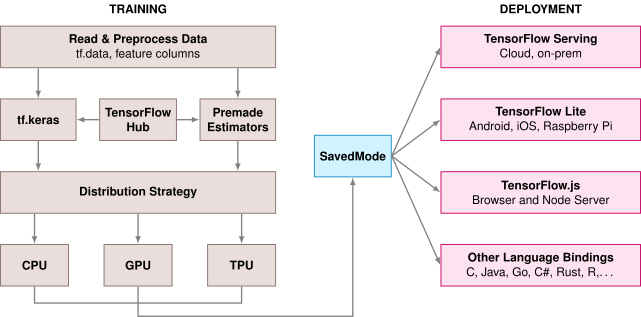](https://mlsysbook.ai/contents/core/frameworks/f56e78010ba72d3921b997fd36aecc250fb6646e.svg "Figure 16: TensorFlow 2.0 Architecture: This diagram outlines TensorFlow’s modular design, separating eager execution from graph construction for increased flexibility and ease of debugging. TensorFlow core provides foundational apis, while Keras serves as its high-level interface for simplified model building and training, supporting deployment across various platforms and hardware accelerators. Source: TensorFlow..")
Figure 16: **TensorFlow 2.0 Architecture**: This diagram outlines TensorFlow’s modular design, separating eager execution from graph construction for increased flexibility and ease of debugging. TensorFlow core provides foundational apis, while Keras serves as its high-level interface for simplified model building and training, supporting deployment across various platforms and hardware accelerators. Source: [TensorFlow.](https://blog.tensorflow.org/2019/01/whats-coming-in-tensorflow-2-0.html)
.
#### Production-Scale Deployment
Real-world production systems demonstrate how framework selection directly impacts system performance under operational constraints. Framework optimization often achieves dramatic improvements: production systems commonly see 4-10x latency reductions and 2-5x cost savings through systematic optimization including quantization, operator fusion, and hardware-specific acceleration.
However, these optimizations require significant engineering investment, typically 4-12 weeks of specialized effort for custom operator implementation, validation testing, and performance tuning. Framework selection emerges as a systems engineering decision that extends far beyond API preferences to encompass the entire optimization and deployment pipeline.
The detailed production deployment examples, optimization techniques, and quantitative trade-off analysis are covered comprehensively in **[Chapter 13: ML Operations](https://mlsysbook.ai/contents/core/ops/ops.html#sec-ml-operations)
**, where operational constraints and deployment strategies are systematically addressed.
### PyTorch
In contrast to TensorFlow’s production-first approach, PyTorch, developed by Facebook’s AI Research lab, has gained significant traction in the machine learning community, particularly among researchers and academics. Its design philosophy emphasizes ease of use, flexibility, and dynamic computation, which aligns well with the iterative nature of research and experimentation.
PyTorch’s research-oriented philosophy manifests in its dynamic computational graph system. Unlike TensorFlow’s traditional static graphs, PyTorch builds computational graphs on-the-fly during execution through its “define-by-run” approach. This enables intuitive model design, easier debugging, and standard Python control flow within models. The dynamic approach supports variable-length inputs and complex architectures while providing immediate execution and inspection capabilities.
PyTorch shares fundamental abstractions with other frameworks, including tensors as the core data structure and seamless CUDA integration for GPU acceleration. The autograd system automatically tracks operations for gradient-based optimization.
### JAX
JAX represents a third distinct approach, developed by Google Research for high-performance numerical computing and advanced machine learning research. Unlike TensorFlow’s static graphs or PyTorch’s dynamic execution, JAX centers on functional programming principles and composition of transformations.
Built as a NumPy-compatible library with automatic differentiation and just-in-time compilation, JAX feels familiar to scientific Python developers while providing powerful optimization tools. JAX can differentiate native Python and NumPy functions, including those with loops, branches, and recursion, extending beyond simple transformations to enable vectorization and JIT compilation.
JAX’s compilation strategy leverages XLA more centrally than TensorFlow, optimizing Python code for various hardware accelerators. The functional programming approach uses pure functions and immutable data, creating predictable, easily optimized code. JAX’s composable transformations include automatic differentiation (grad), vectorization (vmap), and parallel execution (pmap), enabling powerful operations that distinguish it from imperative frameworks.
### Quantitative Platform Performance Analysis
[Table 3](https://mlsysbook.ai/contents/core/frameworks/frameworks.html#tbl-mlfm-comparison)
provides a concise comparison of three major machine learning frameworks: TensorFlow, PyTorch, and JAX. These frameworks, while serving similar purposes, exhibit fundamental differences in their design philosophies and technical implementations.
Table 3: **Framework Characteristics**: TensorFlow, PyTorch, and JAX differ in their graph construction (static, dynamic, or functional), which influences programming style and execution speed. Core distinctions include data mutability (arrays in JAX are immutable) and automatic differentiation capabilities, with JAX supporting both forward and reverse modes. Performance characteristics shown are representative benchmarks that can vary significantly based on workload, hardware configuration, and optimization settings. JAX typically achieves higher GPU utilization and distributed scaling efficiency, while PyTorch offers the most intuitive debugging experience through dynamic graphs.
| | | | |
| --- | --- | --- | --- |
| **Graph Type** | Static (1.x), Dynamic (2.x) | Dynamic | Functional transformations |
| **Programming Model** | Imperative (2.x), Symbolic (1.x) | Imperative | Functional |
| **Core Data Structure** | Tensor (mutable) | Tensor (mutable) | Array (immutable) |
| **Execution Mode** | Eager (2.x default), Graph | Eager | Just-in-time compilation |
| **Automatic Differentiation** | Reverse mode | Reverse mode | Forward and Reverse mode |
| **Hardware Acceleration** | CPU, GPU, TPU | CPU, GPU | CPU, GPU, TPU |
| **Compilation Optimization** | XLA: 3-10x speedup | TorchScript: 2x | XLA: 3-10x speedup |
| **Memory Efficiency** | 85% GPU utilization | 82% GPU util. | 91% GPU utilization |
| **Distributed Scalability** | 92% efficiency (1024 GPUs) | 88% efficiency | 95% efficiency (1024 GPUs) |
These architectural differences manifest in distinct programming paradigms and API design choices. The following example illustrates how the same simple neural network (a single linear layer mapping 10 inputs to 1 output) varies dramatically across these major frameworks, revealing their fundamental design philosophies.
**Example:** Framework Comparison: Hello World
Here’s how the same simple neural network looks across major frameworks to illustrate syntax differences:
# PyTorch - Dynamic, Pythonic
import torch.nn as nn
class SimpleNet(nn.Module):
def __init__(self):
super().__init__()
self.fc = nn.Linear(10, 1)
def forward(self, x):
return self.fc(x)
# TensorFlow/Keras - High-level API
import tensorflow as tf
model = tf.keras.Sequential(
[tf.keras.layers.Dense(1, input_shape=(10,))]
)
# JAX - Functional approach
import jax.numpy as jnp
from jax import random
def simple_net(params, x):
return jnp.dot(x, params["w"]) + params["b"]
key = random.PRNGKey(0)
params = {
"w": random.normal(key, (10, 1)),
"b": random.normal(key, (1,)),
}
The PyTorch implementation exemplifies object-oriented design with explicit class inheritance from `nn.Module`. Developers define model architecture in `__init__()` and computation flow in `forward()`, providing clear separation between structure and execution. This imperative style allows dynamic graph construction where the computational graph is built during execution, enabling flexible control flow and debugging.
In contrast, TensorFlow/Keras demonstrates declarative programming through sequential layer composition. The `Sequential` API abstracts away implementation details, automatically handling layer connections, weight initialization, and forward pass orchestration behind the scenes. When instantiated, Sequential creates a container that manages the computational graph, automatically connecting each layer’s output to the next layer’s input. This approach reflects TensorFlow’s evolution toward eager execution while maintaining compatibility with graph-based optimization for production deployment.
JAX takes a fundamentally different approach, embracing functional programming principles with immutable data structures[28](https://mlsysbook.ai/contents/core/frameworks/frameworks.html#fn28)
and explicit parameter management. The `simple_net` function implements the linear transformation manually using `jnp.dot(x, params['w']) + params['b']`, explicitly performing the matrix multiplication and bias addition that PyTorch and TensorFlow handle automatically. Parameters are stored in a dictionary structure (`params`) containing weights `'w'` and bias `'b'`, initialized separately using JAX’s random number generation with explicit seeding (`random.PRNGKey(0)`). This separation means the model function is stateless[29](https://mlsysbook.ai/contents/core/frameworks/frameworks.html#fn29)
; it contains no parameters internally and depends entirely on external parameter passing. This design enables powerful program transformations like automatic vectorization[30](https://mlsysbook.ai/contents/core/frameworks/frameworks.html#fn30)
(`vmap`), just-in-time compilation[31](https://mlsysbook.ai/contents/core/frameworks/frameworks.html#fn31)
(`jit`), and automatic differentiation (`grad`) because the function remains mathematically pure[32](https://mlsysbook.ai/contents/core/frameworks/frameworks.html#fn32)
without hidden state or side effects.
28 **Immutable Data Structures**: Cannot be modified after creation. Any operation that appears to change the data actually creates a new copy, ensuring that the original data remains unchanged. This prevents accidental modifications and enables safe parallel processing.
29 **Stateless Function**: Produces the same output for the same inputs every time, without relying on or modifying any external state. This predictability is essential for mathematical optimization and parallel execution.
30 **Automatic Vectorization**: Transforms operations on single data points into operations on entire arrays or batches, significantly improving computational efficiency by leveraging SIMD (Single Instruction, Multiple Data) processor capabilities.
31 **Just-in-Time (JIT) Compilation**: Translates high-level code into optimized machine code at runtime, enabling performance optimizations based on actual data shapes and hardware characteristics.
32 **Pure Function**: Has no side effects and always returns the same output for the same inputs. Pure functions enable mathematical reasoning about code behavior and safe program transformations.
### Framework Design Philosophy
Beyond technical specifications, machine learning frameworks embody distinct design philosophies that reflect their creators’ priorities and intended use cases. Understanding these philosophical approaches helps developers choose frameworks that align with their project requirements and working styles. The design philosophy of a framework influences everything from API design to performance characteristics, ultimately affecting both developer productivity and system performance.
#### Research-First Philosophy: PyTorch
PyTorch exemplifies a research-first philosophy, prioritizing developer experience and experimental flexibility over performance optimization. Key design decisions include eager execution for immediate inspection capabilities, embracing Python’s native control structures rather than domain-specific languages, and exposing computational details for precise researcher control. This approach enables rapid prototyping and debugging, driving adoption in academic settings where exploration and experimentation are paramount.
#### Scalability and Deployment-Optimized Design
TensorFlow prioritizes production deployment and scalability, reflecting Google’s experience with massive-scale machine learning systems. This production-first approach emphasizes static graph optimization through XLA compilation, providing 3-10x performance improvements via operation fusion and hardware-specific code generation. The framework includes comprehensive production tools like TensorFlow Serving and TFX, designed for distributed deployment and serving at scale. Higher-level abstractions like Keras prioritize reliability over flexibility, while API evolution emphasizes backward compatibility and gradual migration paths for production stability.
#### Mathematical Transformation and Composability Focus
JAX represents a functional programming approach emphasizing mathematical purity and program transformation capabilities. Immutable arrays and pure functions enable automatic vectorization (`vmap`), parallelization (`pmap`), and differentiation (`grad`) without hidden state concerns. Rather than ML-specific abstractions, JAX provides general program transformations that compose to create complex behaviors, separating computation from execution strategy. While maintaining NumPy compatibility, the functional constraints enable powerful optimization capabilities that make research code mirror mathematical algorithm descriptions.
#### Framework Philosophy Alignment with Project Requirements
These philosophical differences have practical implications for framework selection. Teams engaged in exploratory research often benefit from PyTorch’s research-first philosophy. Organizations focused on deploying models at scale may prefer TensorFlow’s production-first approach. Research groups working on fundamental algorithmic development might choose JAX’s functional approach for program transformation and mathematical reasoning.
Understanding these philosophies helps teams anticipate both current capabilities and future evolution. PyTorch’s research focus suggests continued investment in developer experience. TensorFlow’s production orientation implies ongoing deployment and scaling tool development. JAX’s functional philosophy points toward continued program transformation exploration.
The choice of framework philosophy often has lasting implications for a project’s development trajectory, influencing everything from code organization to debugging workflows to deployment strategies. Teams that align their framework choice with their fundamental priorities and working styles typically achieve better long-term outcomes than those who focus solely on technical specifications.
**Self-Check: Question 1.7**
1. Which of the following frameworks emphasizes a research-first philosophy, prioritizing developer experience and experimental flexibility?
1. TensorFlow
2. JAX
3. PyTorch
4. ONNX
2. Explain how TensorFlow’s production-first philosophy influences its framework design and deployment capabilities.
3. Order the following TensorFlow ecosystem components based on their intended deployment environment: (1) TensorFlow Core, (2) TensorFlow Lite, (3) TensorFlow.js.
4. What is a key advantage of JAX’s functional programming approach over imperative frameworks like TensorFlow and PyTorch?
1. Dynamic computational graphs
2. Automatic vectorization and parallelization
3. High-level API for model building
4. Backward compatibility with earlier versions
[See Answers →](https://mlsysbook.ai/contents/core/frameworks/frameworks.html#quiz-answer-sec-ai-frameworks-major-framework-platform-analysis-6177)
Deployment Environment-Specific Frameworks
------------------------------------------
Beyond the core framework philosophies explored above, machine learning frameworks have evolved significantly to meet the diverse needs of different computational environments. As ML applications expand beyond traditional data centers to encompass edge devices, mobile platforms, and even tiny microcontrollers, the need for specialized frameworks has become increasingly apparent.
This diversification reflects the fundamental challenge of deployment heterogeneity. Framework specialization refers to the process of tailoring ML frameworks to optimize performance, efficiency, and functionality for specific deployment environments. This specialization is crucial because the computational resources, power constraints, and use cases vary dramatically across different platforms.
The proliferation of specialized frameworks creates potential fragmentation challenges that the ML community has addressed through standardization efforts. Machine learning frameworks have addressed interoperability challenges through standardized model formats, with the Open Neural Network Exchange (ONNX)[33](https://mlsysbook.ai/contents/core/frameworks/frameworks.html#fn33)
emerging as a widely adopted solution. ONNX defines a common representation for neural network models that enables seamless translation between different frameworks and deployment environments.
33 **ONNX (Open Neural Network Exchange)**: Industry standard for representing ML models that enables interoperability between frameworks. Supported by Microsoft, Facebook, AWS, and others, ONNX allows models trained in PyTorch to be deployed in TensorFlow Serving or optimized with TensorRT, solving the framework fragmentation problem.
This standardization addresses practical workflow needs. The ONNX format serves two primary purposes. First, it provides a framework-neutral specification for describing model architecture and parameters. Second, it includes runtime implementations that can execute these models across diverse hardware platforms. This standardization eliminates the need to manually convert or reimplement models when moving between frameworks.
In practice, ONNX facilitates important workflow patterns in production machine learning systems. For example, a research team may develop and train a model using PyTorch’s dynamic computation graphs, then export it to ONNX for deployment using TensorFlow’s production-optimized serving infrastructure. Similarly, models can be converted to ONNX format for execution on edge devices using specialized runtimes like ONNX Runtime. This interoperability, illustrated in [Figure 17](https://mlsysbook.ai/contents/core/frameworks/frameworks.html#fig-onnx)
, has become increasingly important as the machine learning ecosystem has expanded. Organizations frequently require leveraging different frameworks’ strengths at various stages of the machine learning lifecycle, from research and development.
[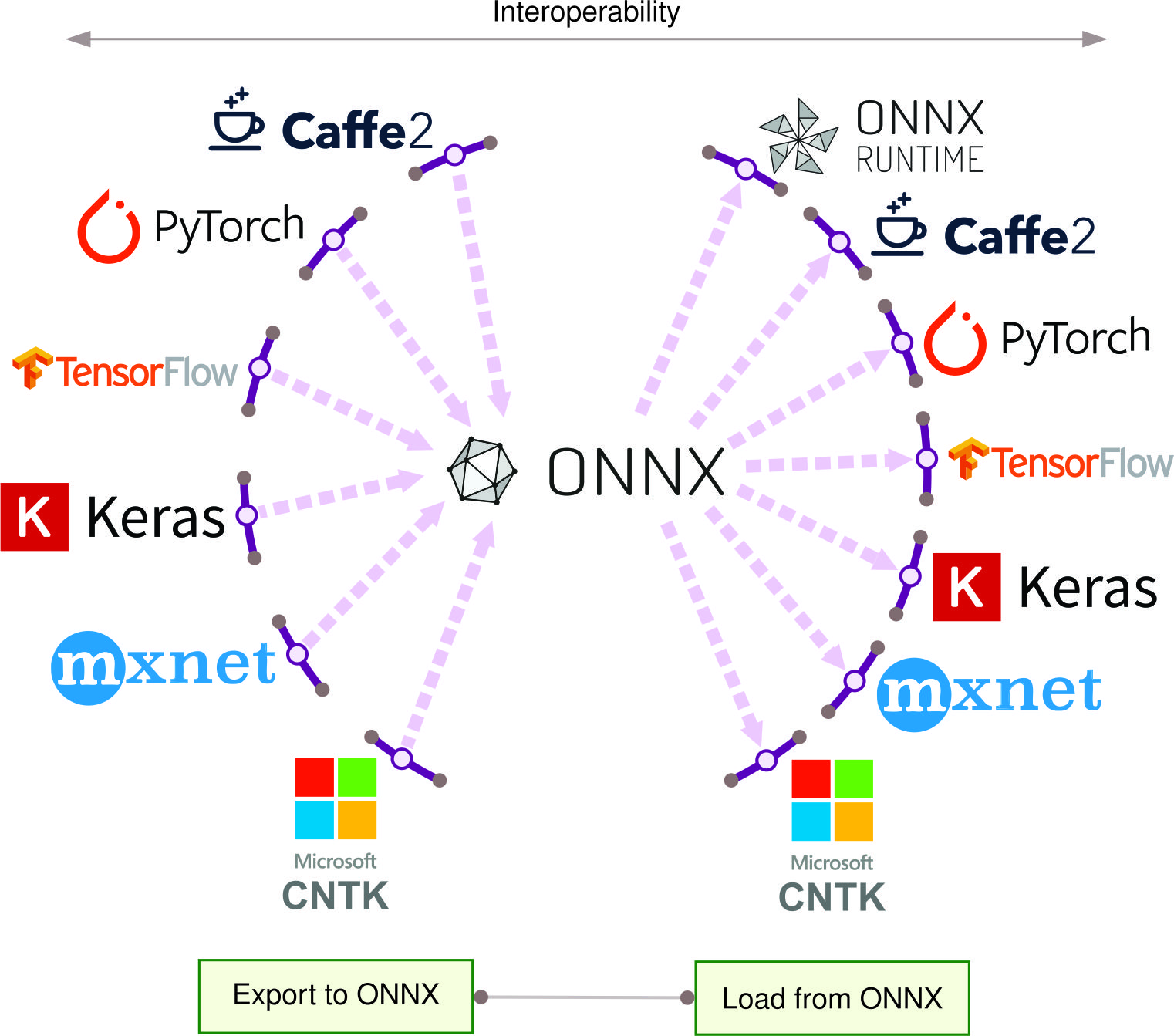](https://mlsysbook.ai/contents/core/frameworks/images/jpeg/onnx_new.jpg "Figure 17: Framework Interoperability: The open neural network exchange (ONNX) format enables model portability across machine learning frameworks, allowing researchers to train models in one framework (e.g., PyTorch) and deploy them using another (e.g., TensorFlow) without code rewriting. This standardization streamlines machine learning workflows and facilitates leveraging specialized runtimes like ONNX runtime for diverse hardware platforms.")
Figure 17: **Framework Interoperability**: The open neural network exchange (ONNX) format enables model portability across machine learning frameworks, allowing researchers to train models in one framework (e.g., PyTorch) and deploy them using another (e.g., TensorFlow) without code rewriting. This standardization streamlines machine learning workflows and facilitates leveraging specialized runtimes like ONNX runtime for diverse hardware platforms.
The diversity of deployment targets necessitates distinct specialization strategies for different environments. Machine learning deployment environments shape how frameworks specialize and evolve. Cloud ML environments leverage high-performance servers that offer abundant computational resources for complex operations. Edge ML operates on devices with moderate computing power, where real-time processing often takes priority. Mobile ML adapts to the varying capabilities and energy constraints of smartphones and tablets. Tiny ML functions within the strict limitations of microcontrollers and other highly constrained devices that possess minimal resources.
These environmental constraints drive specific architectural decisions. Each of these environments presents unique challenges that influence framework design. Cloud frameworks prioritize scalability and distributed computing. Edge frameworks focus on low-latency inference and adaptability to diverse hardware. Mobile frameworks emphasize energy efficiency and integration with device-specific features. TinyML frameworks specialize in extreme resource optimization for severely constrained environments.
We will explore how ML frameworks adapt to each of these environments. We will examine the specific techniques and design choices that enable frameworks to address the unique challenges of each domain, highlighting the trade-offs and optimizations that characterize framework specialization.
### Distributed Computing Platform Optimization
Cloud environments offer the most abundant computational resources, enabling frameworks to prioritize scalability and sophisticated optimizations over resource constraints. Cloud ML frameworks are sophisticated software infrastructures designed to leverage the vast computational resources available in cloud environments. These frameworks specialize in three primary areas: distributed computing architectures, management of large-scale data and models, and integration with cloud-native services.
The first specialization area reflects the scale advantages available in cloud deployments. Distributed computing is a fundamental specialization of cloud ML frameworks. These frameworks implement advanced strategies for partitioning and coordinating computational tasks across multiple machines or graphics processing units (GPUs). This capability is essential for training large-scale models on massive datasets. Both TensorFlow and PyTorch, two leading cloud ML frameworks, offer robust support for distributed computing. TensorFlow’s graph-based approach (in its 1.x version) was particularly well-suited for distributed execution, while PyTorch’s dynamic computational graph allows for more flexible distributed training strategies.
The ability to handle large-scale data and models is another key specialization. Cloud ML frameworks are optimized to work with datasets and models that far exceed the capacity of single machines. This specialization is reflected in the data structures of these frameworks. For instance, both TensorFlow and PyTorch use mutable Tensor objects as their primary data structure, allowing for efficient in-place operations on large datasets. JAX, a more recent framework, uses immutable arrays, which can provide benefits in terms of functional programming paradigms and optimization opportunities in distributed settings.
Integration with cloud-native services is the third major specialization area. This integration enables automated resource scaling, seamless access to cloud storage, and incorporation of cloud-based monitoring and logging systems. The execution modes of different frameworks play a role here. TensorFlow 2.x and PyTorch both default to eager execution, which allows for easier integration with cloud services and debugging. JAX’s just-in-time compilation offers potential performance benefits in cloud environments by optimizing computations for specific hardware.
Hardware acceleration is an important aspect of cloud ML frameworks. All major frameworks support CPU and GPU execution, with TensorFlow and JAX also offering native support for Google’s TPU. [NVIDIA’s TensorRT](https://developer.nvidia.com/tensorrt)
[34](https://mlsysbook.ai/contents/core/frameworks/frameworks.html#fn34)
is an optimization tool dedicated for GPU-based inference, providing sophisticated optimizations like layer fusion, precision calibration, and kernel auto-tuning to maximize throughput on NVIDIA GPUs. These hardware acceleration options allow cloud ML frameworks to efficiently utilize the diverse computational resources available in cloud environments.
34 **TensorRT**: NVIDIA’s inference optimization library that maximizes throughput and minimizes latency for deep learning applications. Achieves 2-5x inference speedup through layer fusion, precision calibration, and kernel auto-tuning, making it essential for production deployment on NVIDIA hardware.
The automatic differentiation capabilities of these frameworks are particularly important in cloud settings where complex models with millions of parameters are common. While TensorFlow and PyTorch primarily use reverse-mode differentiation, JAX’s support for both forward and reverse-mode differentiation can offer advantages in certain large-scale optimization scenarios.
These specializations enable cloud ML frameworks to fully utilize the scalability and computational power of cloud infrastructure. However, this capability comes with increased complexity in deployment and management, often requiring specialized knowledge to fully leverage these frameworks. The focus on scalability and integration makes cloud ML frameworks particularly suitable for large-scale research projects, enterprise-level ML applications, and scenarios requiring massive computational resources.
### Local Processing and Low-Latency Optimization
Moving from the resource-abundant cloud environment to edge deployments introduces significant new constraints that reshape framework priorities. Edge ML frameworks are specialized software tools designed to facilitate machine learning operations in edge computing environments, characterized by proximity to data sources, stringent latency requirements, and limited computational resources. Examples of popular edge ML frameworks include [TensorFlow Lite](https://www.tensorflow.org/lite)
and [Edge Impulse](https://www.edgeimpulse.com/)
. The specialization of these frameworks addresses three primary challenges: real-time inference optimization, adaptation to heterogeneous hardware, and resource-constrained operation. These challenges directly relate to the efficiency techniques discussed in **[Chapter 9: Efficient AI](https://mlsysbook.ai/contents/core/efficient_ai/efficient_ai.html#sec-efficient-ai)
** and require the hardware acceleration strategies covered in **[Chapter 11: AI Acceleration](https://mlsysbook.ai/contents/core/hw_acceleration/hw_acceleration.html#sec-ai-acceleration)
**.
Real-time inference optimization is a critical feature of edge ML frameworks. This often involves leveraging different execution modes and graph types. For instance, while TensorFlow Lite (the edge-focused version of TensorFlow) uses a static graph approach to optimize inference, frameworks like [PyTorch Mobile](https://pytorch.org/mobile/home/)
maintain a dynamic graph capability, allowing for more flexible model structures at the cost of some performance. The choice between static and dynamic graphs in edge frameworks often is a trade-off between optimization potential and model flexibility.
Adaptation to heterogeneous hardware is crucial for edge deployments. Edge ML frameworks extend the hardware acceleration capabilities of their cloud counterparts but with a focus on edge-specific hardware. For instance, TensorFlow Lite supports acceleration on mobile GPUs and edge TPUs, while frameworks like [ARM’s Compute Library](https://developer.arm.com/solutions/machine-learning-on-arm/developer-material/how-to-guides)
optimize for ARM-based processors. This specialization often involves custom operator implementations and low-level optimizations specific to edge hardware.
Operating within resource constraints is another aspect of edge ML framework specialization. This is reflected in the data structures and execution models of these frameworks. For instance, many edge frameworks use quantized tensors as their primary data structure, representing values with reduced precision (e.g., 8-bit integers instead of 32-bit floats) to decrease memory usage and computational demands. These quantization techniques, along with other optimization methods like pruning and knowledge distillation, are explored in detail in **[Chapter 10: Model Optimizations](https://mlsysbook.ai/contents/core/optimizations/optimizations.html#sec-model-optimizations)
**. The automatic differentiation capabilities, while crucial for training in cloud environments, are often stripped down or removed entirely in edge frameworks to reduce model size and improve inference speed.
Edge ML frameworks also often include features for model versioning and updates, allowing for the deployment of new models with minimal system downtime. Some frameworks support limited on-device learning, enabling models to adapt to local data without compromising data privacy. These on-device learning capabilities are explored in depth in **[Chapter 14: On-Device Learning](https://mlsysbook.ai/contents/core/ondevice_learning/ondevice_learning.html#sec-ondevice-learning)
**, while the privacy implications are thoroughly covered in **[Chapter 15: Security & Privacy](https://mlsysbook.ai/contents/core/privacy_security/privacy_security.html#sec-security-privacy)
**.
The specializations of edge ML frameworks collectively enable high-performance inference in resource-constrained environments. This capability expands the potential applications of AI in areas with limited cloud connectivity or where real-time processing is crucial. However, effective utilization of these frameworks requires careful consideration of target hardware specifications and application-specific requirements, necessitating a balance between model accuracy and resource utilization.
### Resource-Constrained Device Optimization
Mobile environments introduce additional constraints beyond those found in general edge computing, particularly regarding energy efficiency and user experience requirements. Mobile ML frameworks are specialized software tools designed for deploying and executing machine learning models on smartphones and tablets. Examples include TensorFlow Lite and [Apple’s Core ML](https://developer.apple.com/documentation/coreml/)
. These frameworks address the unique challenges of mobile environments, including limited computational resources, constrained power consumption, and diverse hardware configurations. The specialization of mobile ML frameworks primarily focuses on on-device inference optimization, energy efficiency, and integration with mobile-specific hardware and sensors.
On-device inference optimization in mobile ML frameworks often involves a careful balance between graph types and execution modes. For instance, TensorFlow Lite, also a popular mobile ML framework, uses a static graph approach to optimize inference performance. This contrasts with the dynamic graph capability of PyTorch Mobile, which offers more flexibility at the cost of some performance. The choice between static and dynamic graphs in mobile frameworks is a trade-off between optimization potential and model adaptability, crucial in the diverse and changing mobile environment.
The data structures in mobile ML frameworks are optimized for efficient memory usage and computation. While cloud-based frameworks like TensorFlow and PyTorch use mutable tensors, mobile frameworks often employ more specialized data structures. For example, many mobile frameworks use quantized tensors, representing values with reduced precision (e.g., 8-bit integers instead of 32-bit floats) to decrease memory footprint and computational demands. This specialization is critical given the limited RAM and processing power of mobile devices.
Energy efficiency, a key concern in mobile environments, influences the design of execution modes in mobile ML frameworks. Unlike cloud frameworks that may use eager execution for ease of development, mobile frameworks often prioritize graph-based execution for its potential energy savings. For instance, Apple’s Core ML uses a compiled model approach, converting ML models into a form that can be efficiently executed by iOS devices, optimizing for both performance and energy consumption.
Integration with mobile-specific hardware and sensors is another key specialization area. Mobile ML frameworks extend the hardware acceleration capabilities of their cloud counterparts but with a focus on mobile-specific processors. For example, TensorFlow Lite can leverage mobile GPUs and neural processing units (NPUs) found in many modern smartphones. Qualcomm’s Neural Processing SDK is designed to efficiently utilize the AI accelerators present in Snapdragon SoCs. This hardware-specific optimization often involves custom operator implementations and low-level optimizations tailored for mobile processors.
Automatic differentiation, while crucial for training in cloud environments, is often minimized or removed entirely in mobile frameworks to reduce model size and improve inference speed. Instead, mobile ML frameworks focus on efficient inference, with model updates typically performed off-device and then deployed to the mobile application.
Mobile ML frameworks also often include features for model updating and versioning, allowing for the deployment of improved models without requiring full app updates. Some frameworks support limited on-device learning, enabling models to adapt to user behavior or environmental changes without compromising data privacy. The technical approaches and implementation strategies for on-device learning are detailed in **[Chapter 14: On-Device Learning](https://mlsysbook.ai/contents/core/ondevice_learning/ondevice_learning.html#sec-ondevice-learning)
**, while privacy preservation techniques are covered in **[Chapter 15: Security & Privacy](https://mlsysbook.ai/contents/core/privacy_security/privacy_security.html#sec-security-privacy)
**.
The specializations of mobile ML frameworks collectively enable the deployment of sophisticated ML models on resource-constrained mobile devices. This expands the potential applications of AI in mobile environments, ranging from real-time image and speech recognition to personalized user experiences. However, effectively utilizing these frameworks requires careful consideration of the target device capabilities, user experience requirements, and privacy implications, necessitating a balance between model performance and resource utilization.
### Microcontroller and Embedded System Implementation
At the extreme end of the resource constraint spectrum, TinyML frameworks operate under conditions that push the boundaries of what is computationally feasible. TinyML frameworks are specialized software infrastructures designed for deploying machine learning models on extremely resource-constrained devices, typically microcontrollers and low-power embedded systems. These frameworks address the severe limitations in processing power, memory, and energy consumption characteristic of tiny devices. The specialization of TinyML frameworks primarily focuses on extreme model compression, optimizations for severely constrained environments, and integration with microcontroller-specific architectures.
Extreme model compression in TinyML frameworks takes the quantization techniques mentioned in mobile and edge frameworks to their logical conclusion. While mobile frameworks might use 8-bit quantization, TinyML often employs even more aggressive techniques, such as 4-bit, 2-bit, or even 1-bit (binary) representations of model parameters. Frameworks like TensorFlow Lite Micro exemplify this approach ([David et al. 2021](https://mlsysbook.ai/contents/core/frameworks/frameworks.html#ref-david2021tensorflow)
), pushing the boundaries of model compression to fit within the kilobytes of memory available on microcontrollers.
David, Robert, Jared Duke, Advait Jain, Vijay Janapa Reddi, Nat Jeffries, Jian Li, Nick Kreeger, et al. 2021. “Tensorflow Lite Micro: Embedded Machine Learning for Tinyml Systems.” _Proceedings of Machine Learning and Systems_ 3: 800–811.
The execution model in TinyML frameworks is highly specialized. Unlike the dynamic graph capabilities seen in some cloud and mobile frameworks, TinyML frameworks almost exclusively use static, highly optimized graphs. The just-in-time compilation approach seen in frameworks like JAX is typically not feasible in TinyML due to memory constraints. Instead, these frameworks often employ ahead-of-time compilation techniques to generate highly optimized, device-specific code.
Memory management in TinyML frameworks is far more constrained than in other environments. While edge and mobile frameworks might use dynamic memory allocation, TinyML frameworks like [uTensor](https://github.com/uTensor/uTensor)
often rely on static memory allocation to avoid runtime overhead and fragmentation. This approach requires careful planning of the memory layout at compile time, a stark contrast to the more flexible memory management in cloud-based frameworks.
Hardware integration in TinyML frameworks is highly specific to microcontroller architectures. Unlike the general GPU support seen in cloud frameworks or the mobile GPU/NPU support in mobile frameworks, TinyML frameworks often provide optimizations for specific microcontroller instruction sets. For example, ARM’s CMSIS-NN ([Lai, Suda, and Chandra 2018](https://mlsysbook.ai/contents/core/frameworks/frameworks.html#ref-lai2018cmsis)
) provides optimized neural network kernels for Cortex-M series microcontrollers, which are often integrated into TinyML frameworks.
Lai, Liangzhen, Naveen Suda, and Vikas Chandra. 2018. “CMSIS-NN: Efficient Neural Network Kernels for Arm Cortex-m CPUs.” _ArXiv Preprint_ abs/1801.06601 (January). [http://arxiv.org/abs/1801.06601v1](http://arxiv.org/abs/1801.06601v1)
.
The concept of automatic differentiation, central to cloud-based frameworks and present to some degree in edge and mobile frameworks, is typically absent in TinyML frameworks. The focus is almost entirely on inference, with any learning or model updates usually performed off-device due to the severe computational constraints.
TinyML frameworks also specialize in power management to a degree not seen in other ML environments. Features like duty cycling and ultra-low-power wake-up capabilities are often integrated directly into the ML pipeline, enabling always-on sensing applications that can run for years on small batteries.
The extreme specialization of TinyML frameworks enables ML deployments in previously infeasible environments, from smart dust sensors to implantable medical devices. However, this specialization comes with significant trade-offs in model complexity and accuracy, requiring careful consideration of the balance between ML capabilities and the severe resource constraints of target devices.
### Performance and Resource Optimization Platforms
Beyond deployment-specific specializations, modern machine learning frameworks increasingly incorporate efficiency as a first-class design principle. Efficiency-oriented frameworks are specialized tools that treat computational efficiency, memory optimization, and energy consumption as primary design constraints rather than secondary considerations. These frameworks address the growing demand for practical AI deployment where resource constraints fundamentally shape algorithmic choices.
Traditional frameworks often treat efficiency optimizations as optional add-ons, applied after model development. In contrast, efficiency-oriented frameworks integrate optimization techniques directly into the development workflow, enabling developers to train and deploy models with quantization, pruning, and compression constraints from the beginning. This efficiency-first approach enables deployment scenarios where traditional frameworks would be computationally infeasible.
The significance of efficiency-oriented frameworks has grown with the expansion of AI applications into resource-constrained environments. Modern production systems require models that balance accuracy with strict constraints on inference latency (often sub-10ms requirements), memory usage (fitting within GPU memory limits), energy consumption (extending battery life), and computational cost (reducing cloud infrastructure expenses). These constraints create substantially different framework requirements compared to research environments with abundant computational resources.
#### Model Size and Computational Reduction Techniques
Efficiency-oriented frameworks distinguish themselves through compression-aware computational graph design. Unlike traditional frameworks that optimize mathematical operations independently, these frameworks optimize for compressed representations throughout the computation pipeline. This integration affects every layer of the framework stack, from data structures to execution engines.
Neural network compression techniques require framework support for specialized data types and operations. Quantization-aware training demands frameworks that can simulate reduced precision arithmetic during training while maintaining full-precision gradients for stable optimization. Intel Neural Compressor exemplifies this approach, providing APIs that seamlessly integrate INT8 quantization into existing PyTorch and TensorFlow workflows. The framework automatically inserts fake quantization operations during training, allowing models to adapt to quantization constraints while preserving accuracy.
Structured pruning techniques require frameworks that can handle sparse tensor operations efficiently. This involves specialized storage formats (such as compressed sparse row representations), optimized sparse matrix operations, and runtime systems that can take advantage of structural zeros. Apache TVM demonstrates advanced sparse tensor compilation, automatically generating efficient code for sparse operations across different hardware backends.
Knowledge distillation workflows represent another efficiency-oriented framework capability. These frameworks must orchestrate teacher-student training pipelines, managing the computational overhead of running multiple models simultaneously while providing APIs for custom distillation losses. Hugging Face Optimum provides comprehensive distillation workflows that automatically configure teacher-student training for various model architectures, reducing the engineering complexity of implementing efficiency optimizations.
#### Integrated Hardware-Framework Performance Tuning
Efficiency-oriented frameworks excel at hardware-software co-design, where framework architecture and hardware capabilities are optimized together. This approach moves beyond generic hardware acceleration to target-specific optimization strategies that consider hardware constraints during algorithmic design.
Mixed-precision training frameworks demonstrate this co-design philosophy. NVIDIA’s Automatic Mixed Precision (AMP) in PyTorch automatically identifies operations that can use FP16 arithmetic while maintaining FP32 precision for numerical stability. The framework analyzes computational graphs to determine optimal precision policies, balancing training speed improvements (up to 1.5-2x speedup on modern GPUs) against numerical accuracy requirements. This analysis requires deep integration between framework scheduling and hardware capabilities.
Sparse computation frameworks extend this co-design approach to leverage hardware sparsity support. Modern hardware like NVIDIA A100 GPUs includes specialized sparse matrix multiplication units that can achieve 2:4 structured sparsity (50% zeros in specific patterns) with minimal performance degradation. Frameworks like Neural Magic’s SparseML provide automated tools for training models that conform to these hardware-specific sparsity patterns, achieving significant speedups without accuracy loss.
Compilation frameworks represent the most sophisticated form of hardware-software co-design. Apache TVM and MLIR provide domain-specific languages for expressing hardware-specific optimizations. These frameworks analyze computational graphs to automatically generate optimized kernels for specific hardware targets, including custom ASICs and specialized accelerators. The compilation process considers hardware memory hierarchies, instruction sets, and parallelization capabilities to generate code that often outperforms hand-optimized implementations.
#### Real-World Deployment Performance Requirements
Efficiency-oriented frameworks address production deployment challenges through systematic approaches to resource management and performance optimization. Production environments impose strict constraints that differ substantially from research settings: inference latency must meet real-time requirements, memory usage must fit within allocated resources, and energy consumption must stay within power budgets.
Inference optimization frameworks like NVIDIA TensorRT and ONNX Runtime provide comprehensive toolchains for production deployment. TensorRT applies aggressive optimization techniques including layer fusion (combining multiple operations into single kernels), precision calibration (automatically determining optimal quantization levels), and memory optimization (reducing memory transfers between operations). These optimizations can achieve 3-7x inference speedup compared to unoptimized frameworks while maintaining accuracy within acceptable bounds.
Memory optimization represents a critical production constraint. DeepSpeed and FairScale demonstrate advanced memory management techniques that enable training and inference of models that exceed GPU memory capacity. DeepSpeed’s ZeRO optimizer partitions optimizer states, gradients, and parameters across multiple devices, reducing memory usage by 4-8x compared to traditional data parallelism. These techniques enable training of models with hundreds of billions of parameters on standard hardware configurations.
Energy-aware frameworks address the growing importance of computational sustainability. Power consumption directly impacts deployment costs in cloud environments and battery life in mobile applications. Frameworks like NVIDIA’s Triton Inference Server provide power-aware scheduling that can dynamically adjust inference batching and frequency scaling to meet energy budgets while maintaining throughput requirements.
#### Systematic Performance Assessment Methodologies
Evaluating efficiency-oriented frameworks requires comprehensive metrics that capture the multi-dimensional trade-offs between accuracy, performance, and resource consumption. Traditional ML evaluation focuses primarily on accuracy metrics, but efficiency evaluation must consider computational efficiency (FLOPS reduction, inference speedup), memory efficiency (peak memory usage, memory bandwidth utilization), energy efficiency (power consumption, energy per inference), and deployment efficiency (model size reduction, deployment complexity).
Quantitative framework comparison requires standardized benchmarks that measure these efficiency dimensions across representative workloads. MLPerf Inference provides standardized benchmarks for measuring inference performance across different frameworks and hardware configurations. These benchmarks measure latency, throughput, and energy consumption for common model architectures, enabling direct comparison of framework efficiency characteristics.
Performance profiling frameworks enable developers to understand efficiency bottlenecks in their specific applications. NVIDIA Nsight Systems and Intel VTune provide detailed analysis of framework execution, identifying memory bandwidth limitations, computational bottlenecks, and opportunities for optimization. These tools integrate with efficiency-oriented frameworks to provide actionable insights for improving application performance.
The evolution of efficiency-oriented frameworks represents a fundamental shift in ML systems design, where computational constraints shape algorithmic choices from the beginning of development. This approach enables practical AI deployment across resource-constrained environments while maintaining the flexibility and expressiveness that makes modern ML frameworks powerful development tools.
**Self-Check: Question 1.8**
1. Which of the following best describes the primary purpose of framework specialization in machine learning?
1. To create a unified framework for all deployment environments
2. To optimize performance and efficiency for specific deployment environments
3. To simplify the development process by reducing the number of frameworks
4. To enhance the theoretical understanding of machine learning algorithms
2. Explain how ONNX addresses interoperability challenges in machine learning frameworks.
3. The \_\_\_\_\_\_\_\_ format enables model portability across machine learning frameworks, allowing seamless translation between different frameworks and deployment environments.
4. In a production system, what trade-offs might you consider when choosing between cloud-based and edge-based ML frameworks?
[See Answers →](https://mlsysbook.ai/contents/core/frameworks/frameworks.html#quiz-answer-sec-ai-frameworks-deployment-environmentspecific-frameworks-f333)
Systematic Framework Selection Methodology
------------------------------------------
Choosing the right machine learning framework requires a systematic evaluation that balances technical requirements with operational constraints. This decision-making process extends beyond simple feature comparisons to encompass the entire system lifecycle, from development through deployment and maintenance. Engineers must evaluate multiple interdependent factors: technical capabilities (supported operations, execution models, hardware targets), operational requirements (deployment constraints, performance needs, scalability demands), and organizational factors (team expertise, development timeline, maintenance resources).
The framework selection process follows a structured approach that considers three primary dimensions: model requirements determine which operations and architectures the framework must support, software dependencies define operating system and runtime requirements, and hardware constraints establish memory and processing limitations. These technical considerations must be balanced with practical factors like team expertise, learning curve, community support, and long-term maintenance commitments.
This decision-making process must also consider the broader system architecture principles outlined in **[Chapter 2: ML Systems](https://mlsysbook.ai/contents/core/ml_systems/ml_systems.html#sec-ml-systems)
** and align with the deployment patterns detailed in **[Chapter 13: ML Operations](https://mlsysbook.ai/contents/core/ops/ops.html#sec-ml-operations)
**. Different deployment scenarios often favor different framework architectures: cloud training requires high throughput and distributed capabilities, edge inference prioritizes low latency and minimal resource usage, mobile deployment balances performance with battery constraints, and embedded systems optimize for minimal memory footprint and real-time execution.
To illustrate how these factors interact in practice, we examine the TensorFlow ecosystem, which demonstrates the spectrum of trade-offs through its variants: TensorFlow, TensorFlow Lite, and TensorFlow Lite Micro. While TensorFlow serves as our detailed case study, the same selection methodology applies broadly across the framework landscape, including PyTorch for research-oriented workflows, ONNX for cross-platform deployment, JAX for functional programming approaches, and specialized frameworks for specific domains.
[Table 4](https://mlsysbook.ai/contents/core/frameworks/frameworks.html#tbl-tf-comparison)
illustrates key differences between TensorFlow variants. Each variant represents specific trade-offs between computational capability and resource requirements. These trade-offs manifest in supported operations, binary size, and integration requirements.
Table 4: **TensorFlow Variant Trade-Offs**: TensorFlow, TensorFlow lite, and TensorFlow lite micro represent a spectrum of design choices balancing model expressiveness, binary size, and resource constraints for diverse deployment scenarios. Supported operations decrease from approximately 1400 in full TensorFlow to 50 in TensorFlow lite micro, reflecting a shift from training capability to efficient inference on edge devices; native quantization tooling enables further optimization for resource-constrained environments.
| | | | |
| --- | --- | --- | --- |
| **Training** | Yes | No | No |
| **Inference** | Yes (_but inefficient on edge_) | Yes (_and efficient_) | Yes (_and even more efficient_) |
| **How Many Ops** | ~1400 | ~130 | ~50 |
| **Native Quantization Tooling** | No | Yes | Yes |
Engineers analyze three primary aspects when selecting a framework:
1. Model requirements determine which operations and architectures the framework must support
2. Software dependencies define operating system and runtime requirements
3. Hardware constraints establish memory and processing limitations
This systematic analysis enables engineers to select frameworks that align with their specific deployment requirements and organizational context. As we examine the TensorFlow variants in detail, we will explore how each selection dimension influences framework choice and shapes system capabilities, providing a methodology that can be applied to evaluate any framework ecosystem.
### Model Requirements
Model architecture capabilities vary significantly across TensorFlow variants, with clear trade-offs between functionality and efficiency. [Table 4](https://mlsysbook.ai/contents/core/frameworks/frameworks.html#tbl-tf-comparison)
quantifies these differences across four key dimensions: training capability, inference efficiency, operation support, and quantization features.
Dynamic vs Static Computational Graphs
A key architectural distinction between frameworks is their computational graph construction approach. Static graphs (TensorFlow 1.x) require defining the entire computation before execution, similar to compiling a program before running it. Dynamic graphs (PyTorch, TensorFlow 2.x eager mode) build the graph during execution, akin to interpreted languages. This affects debugging ease (dynamic graphs allow standard Python debugging), optimization opportunities (static graphs enable more aggressive optimization), and deployment complexity (static graphs simplify deployment but require more upfront design).
TensorFlow supports approximately 1,400 operations and enables both training and inference. However, as [Table 4](https://mlsysbook.ai/contents/core/frameworks/frameworks.html#tbl-tf-comparison)
indicates, its inference capabilities are inefficient for edge deployment. TensorFlow Lite reduces the operation count to roughly 130 operations while improving inference efficiency. It eliminates training support but adds native quantization tooling. TensorFlow Lite Micro further constrains the operation set to approximately 50 operations, achieving even higher inference efficiency through these constraints. Like TensorFlow Lite, it includes native quantization support but removes training capabilities.
This progressive reduction in operations enables deployment on increasingly constrained devices. The addition of native quantization in both TensorFlow Lite and TensorFlow Lite Micro provides essential optimization capabilities absent in the full TensorFlow framework. Quantization transforms models to use lower precision operations, reducing computational and memory requirements for resource-constrained deployments. These optimization techniques, detailed further in **[Chapter 10: Model Optimizations](https://mlsysbook.ai/contents/core/optimizations/optimizations.html#sec-model-optimizations)
**, must be considered alongside data pipeline requirements discussed in **[Chapter 6: Data Engineering](https://mlsysbook.ai/contents/core/data_engineering/data_engineering.html#sec-data-engineering)
** when selecting appropriate frameworks for specific deployment scenarios.
### Software Dependencies
[Table 5](https://mlsysbook.ai/contents/core/frameworks/frameworks.html#tbl-tf-sw-comparison)
reveals three key software considerations that differentiate TensorFlow variants: operating system requirements, memory management capabilities, and accelerator support. These differences reflect each variant’s optimization for specific deployment
Table 5: **TensorFlow Variant Trade-Offs**: TensorFlow, TensorFlow lite, and TensorFlow lite micro offer different capabilities regarding operating system dependence, memory management, and hardware acceleration, reflecting design choices for diverse deployment scenarios. These distinctions enable developers to select the variant best suited for resource-constrained devices or full-scale server deployments, balancing functionality with efficiency.
| | | | |
| --- | --- | --- | --- |
| **Needs an OS** | Yes | Yes | No |
| **Memory Mapping of Models** | No | Yes | Yes |
| **Delegation to accelerators** | Yes | Yes | No |
Operating system dependencies mark a fundamental distinction between variants. TensorFlow and TensorFlow Lite require an operating system, while TensorFlow Lite Micro operates without OS support. This enables TensorFlow Lite Micro to reduce memory overhead and startup time, though it can still integrate with real-time operating systems like FreeRTOS, Zephyr, and Mbed OS when needed.
Memory management capabilities also distinguish the variants. TensorFlow Lite and TensorFlow Lite Micro support model memory mapping, enabling direct model access from flash storage rather than loading into RAM. TensorFlow lacks this capability, reflecting its design for environments with abundant memory resources. Memory mapping becomes increasingly important as deployment moves toward resource-constrained devices.
Accelerator delegation capabilities further differentiate the variants. Both TensorFlow and TensorFlow Lite support delegation to accelerators, enabling efficient computation distribution. TensorFlow Lite Micro omits this feature, acknowledging the limited availability of specialized accelerators in embedded systems. This design choice maintains the framework’s minimal footprint while matching typical embedded hardware configurations.
### Hardware Constraints
[Table 6](https://mlsysbook.ai/contents/core/frameworks/frameworks.html#tbl-tf-hw-comparison)
quantifies the hardware requirements across TensorFlow variants through three metrics: base binary size, memory footprint, and processor architecture support. These metrics demonstrate the progressive optimization for constrained computing environments.
Table 6: **TensorFlow Hardware Optimization**: TensorFlow variants exhibit decreasing resource requirements (binary size and memory footprint) as they target increasingly constrained hardware architectures, enabling deployment on devices ranging from servers to microcontrollers. Optimized architectures reflect this trend, shifting from general-purpose cpus and gpus to arm cortex-m processors and digital signal processors for resource-limited environments.
| | | | |
| --- | --- | --- | --- |
| **Base Binary Size** | ~3-5 MB (varies by platform and build configuration) | 100 KB | ~10 KB |
| **Base Memory Footprint** | ~5+ MB (minimum runtime overhead) | 300 KB | 20 KB |
| **Optimized Architectures** | X86, TPUs, GPUs | Arm Cortex A, x86 | Arm Cortex M, DSPs, MCUs |
As established in [Table 4](https://mlsysbook.ai/contents/core/frameworks/frameworks.html#tbl-tf-comparison)
, binary size decreases dramatically across variants: from 3+ MB (TensorFlow) to 100 KB (TensorFlow Lite) to 10 KB (TensorFlow Lite Micro), reflecting progressive feature reduction and optimization.
Memory footprint follows a similar pattern of reduction. TensorFlow requires approximately 5 MB of base memory, while TensorFlow Lite operates within 300 KB. TensorFlow Lite Micro further reduces memory requirements to 20 KB, enabling deployment on highly constrained devices.
Processor architecture support aligns with each variant’s intended deployment environment. TensorFlow supports x86 processors and accelerators including TPUs and GPUs, enabling high-performance computing in data centers as detailed in **[Chapter 11: AI Acceleration](https://mlsysbook.ai/contents/core/hw_acceleration/hw_acceleration.html#sec-ai-acceleration)
**. TensorFlow Lite targets mobile and edge processors, supporting Arm Cortex-A and x86 architectures. TensorFlow Lite Micro specializes in microcontroller deployment, supporting Arm Cortex-M cores, digital signal processors (DSPs), and various microcontroller units (MCUs) including STM32, NXP Kinetis, and Microchip AVR. The hardware acceleration strategies and architectures discussed in **[Chapter 11: AI Acceleration](https://mlsysbook.ai/contents/core/hw_acceleration/hw_acceleration.html#sec-ai-acceleration)
** provide essential context for understanding these processor optimization choices.
### Production-Ready Evaluation Factors
Framework selection for embedded systems extends beyond technical specifications of model architecture, hardware requirements, and software dependencies. Additional factors affect development efficiency, maintenance requirements, and deployment success. Framework migration presents significant operational challenges including backward compatibility breaks, custom operator migration between versions, and production downtime risks. These migration concerns are addressed comprehensively in **[Chapter 13: ML Operations](https://mlsysbook.ai/contents/core/ops/ops.html#sec-ml-operations)
**, which covers migration planning, testing procedures, and rollback strategies. These factors require systematic evaluation to ensure optimal framework selection.
#### Performance Optimization
Performance in embedded systems encompasses multiple metrics beyond computational speed. Framework evaluation must consider quantitative trade-offs across efficiency dimensions:
Inference latency determines system responsiveness and real-time processing capabilities. For mobile applications, typical targets are 10-50ms for image classification and 1-5ms for keyword spotting. Edge deployments often require sub-millisecond response times for industrial control applications. TensorFlow Lite achieves 2-5x latency reduction compared to TensorFlow on mobile CPUs for typical inference workloads, while specialized frameworks like TensorRT can achieve 10-20x speedup on NVIDIA hardware through kernel fusion and precision optimization.
Memory utilization affects both static storage requirements and runtime efficiency. Framework memory overhead varies dramatically: TensorFlow requires 5+ MB baseline memory, TensorFlow Lite operates within 300KB, while TensorFlow Lite Micro runs in 20KB. Model memory scaling follows similar patterns: a MobileNetV2 model consumes approximately 14MB in TensorFlow but only 3.4MB when quantized in TensorFlow Lite, representing a 4x reduction while maintaining 95%+ accuracy.
Power consumption impacts battery life and thermal management requirements. Quantized INT8 inference consumes 4-8x less energy than FP32 operations on typical mobile processors. Apple’s Neural Engine achieves 7.2 TOPS/W efficiency for INT8 operations compared to 0.1-0.5 TOPS/W for CPU-based FP32 computation. Sparse computation can provide additional 2-3x energy savings when frameworks support structured sparsity patterns optimized for specific hardware.
Computational efficiency measured in FLOPS provides standardized performance comparison. Modern mobile frameworks achieve 10-50 GFLOPS on high-end smartphone processors, while specialized accelerators like Google’s Edge TPU deliver 4 TOPS (INT8) in 2W power budget. Framework optimization techniques including operator fusion can improve FLOPS utilization from 10-20% to 60-80% of theoretical peak performance on typical workloads.
#### Deployment Scalability
Scalability requirements span both technical capabilities and operational considerations. Framework support must extend across deployment scales and scenarios:
Device scaling enables consistent deployment from microcontrollers to more powerful embedded processors. Operational scaling supports the transition from development prototypes to production deployments. Version management facilitates model updates and maintenance across deployed devices. The framework must maintain consistent performance characteristics throughout these scaling dimensions.
The TensorFlow ecosystem demonstrates how framework design must balance competing requirements across diverse deployment scenarios. The systematic evaluation methodology illustrated through this case study (analyzing model requirements, software dependencies, and hardware constraints alongside operational factors) provides a template for evaluating any framework ecosystem. Whether comparing PyTorch’s dynamic execution model for research workflows, ONNX’s cross-platform standardization for deployment flexibility, JAX’s functional programming approach for performance optimization, or specialized frameworks for domain-specific applications, the same analytical framework guides informed decision-making that aligns technical capabilities with project requirements and organizational constraints.
### Development Support and Long-term Viability Assessment
Framework selection extends beyond technical capabilities to encompass the broader ecosystem that determines long-term viability and development velocity. The community and ecosystem surrounding a framework significantly influence its evolution, support quality, and integration possibilities. Understanding these ecosystem dynamics helps predict framework sustainability and development productivity over project lifecycles.
#### Developer Resources and Knowledge Sharing Networks
The vitality of a framework’s community affects multiple practical aspects of development and deployment. Active communities drive faster bug fixes, more comprehensive documentation, and broader hardware support. Community size and engagement metrics (such as GitHub activity, Stack Overflow question volume, and conference presence) provide indicators of framework momentum and longevity.
PyTorch’s academic community has driven rapid innovation in research-oriented features, contributing to extensive support for novel architectures and experimental techniques. This community focus has resulted in excellent educational resources, research reproducibility tools, and advanced feature development. However, production tooling has historically lagged behind research capabilities, though initiatives like PyTorch Lightning and TorchServe have addressed many operational gaps.
TensorFlow’s enterprise community has emphasized production-ready tools and scalable deployment solutions. This focus has produced robust serving infrastructure, comprehensive monitoring tools, and enterprise integration capabilities. The broader TensorFlow ecosystem includes specialized tools like TensorFlow Extended (TFX) for production ML pipelines, TensorBoard for visualization, and TensorFlow Model Analysis for model evaluation and validation.
JAX’s functional programming community has concentrated on mathematical rigor and program transformation capabilities. This specialized focus has led to powerful research tools and elegant mathematical abstractions, but with a steeper learning curve for developers not familiar with functional programming concepts.
#### Supporting Infrastructure and Third-Party Compatibility
The practical utility of a framework often depends more on its ecosystem tools than its core capabilities. These tools determine development velocity, debugging effectiveness, and deployment flexibility.
Hugging Face has become a de facto standard for natural language processing model libraries, providing consistent APIs across PyTorch, TensorFlow, and JAX backends. The availability of high-quality pretrained models and fine-tuning tools can dramatically accelerate project development. TensorFlow Hub and PyTorch Hub provide official model repositories, though third-party collections often offer broader selection and more recent architectures.
PyTorch Lightning has abstracted much of PyTorch’s training boilerplate while maintaining research flexibility, addressing one of PyTorch’s historical weaknesses in structured training workflows. Weights & Biases and MLflow provide experiment tracking across multiple frameworks, enabling consistent workflow management regardless of underlying framework choice. TensorBoard has evolved into a cross-framework visualization tool, though its integration remains tightest with TensorFlow.
TensorFlow Serving and TorchServe provide production-ready serving solutions, though their feature sets and operational characteristics differ significantly. ONNX Runtime has emerged as a framework-agnostic serving solution, enabling deployment flexibility at the cost of some framework-specific optimizations. Cloud provider ML services (AWS SageMaker, Google AI Platform, Azure ML) often provide native integration for specific frameworks while supporting others through containerized deployments.
Framework-specific optimization tools can provide significant performance advantages but create vendor lock-in. TensorFlow’s XLA compiler and PyTorch’s TorchScript offer framework-native optimization paths, while tools like Apache TVM provide cross-framework optimization capabilities. The choice between framework-specific and cross-framework optimization tools affects both performance and deployment flexibility.
#### Long-term Technology Investment Considerations
Long-term framework decisions must consider ecosystem evolution and sustainability. Framework popularity can shift rapidly in response to technical innovations, community momentum, or corporate strategy changes. Organizations should evaluate ecosystem health through multiple indicators: contributor diversity (avoiding single-company dependence), funding stability, roadmap transparency, and backward compatibility commitments.
The ecosystem perspective also influences hiring and team development strategies. Framework choice affects the available talent pool, training requirements, and knowledge transfer capabilities. Teams must consider whether their framework choice aligns with local expertise, educational institution curricula, and industry hiring trends.
Integration with existing organizational tools and processes represents another critical ecosystem consideration. Framework compatibility with continuous integration systems, deployment pipelines, monitoring infrastructure, and security tooling can significantly affect operational overhead. Some frameworks integrate more naturally with specific cloud providers or enterprise software stacks, creating operational advantages or vendor dependencies.
While deep ecosystem integration can provide development velocity advantages, teams should maintain awareness of migration paths and cross-framework compatibility. Using standardized model formats like ONNX, maintaining framework-agnostic data pipelines, and documenting framework-specific customizations can preserve flexibility for future framework transitions.
The ecosystem perspective reminds us that framework selection involves choosing not just a software library, but joining a community and committing to an evolving technological ecosystem. Understanding these broader implications helps teams make framework decisions that remain viable and advantageous throughout project lifecycles.
**Self-Check: Question 1.9**
1. Which of the following is a primary consideration when selecting a machine learning framework for deployment on resource-constrained devices?
1. Inference efficiency
2. Training capability
3. Number of supported operations
4. Community support
2. Explain how the choice between TensorFlow and TensorFlow Lite impacts deployment on mobile devices.
3. Order the following framework selection criteria from most to least important for deploying on an embedded system: (1) Hardware constraints, (2) Model requirements, (3) Software dependencies.
4. What is a key advantage of using TensorFlow Lite Micro over TensorFlow Lite for microcontroller deployments?
1. Supports more operations
2. Offers better community support
3. Includes training capabilities
4. Does not require an operating system
[See Answers →](https://mlsysbook.ai/contents/core/frameworks/frameworks.html#quiz-answer-sec-ai-frameworks-systematic-framework-selection-methodology-530e)
Systematic Framework Performance Assessment
-------------------------------------------
Systematic evaluation of framework efficiency requires comprehensive metrics that capture the multi-dimensional trade-offs between accuracy, performance, and resource consumption. Traditional machine learning evaluation focuses primarily on accuracy metrics, but production deployment demands systematic assessment of computational efficiency, memory utilization, energy consumption, and operational constraints.
Framework efficiency evaluation encompasses four primary dimensions that reflect real-world deployment requirements. Computational efficiency measures the framework’s ability to utilize available hardware resources effectively, typically quantified through FLOPS utilization, kernel efficiency, and parallelization effectiveness. Memory efficiency evaluates both peak memory usage and memory bandwidth utilization, critical factors for deployment on resource-constrained devices. Energy efficiency quantifies power consumption characteristics, essential for mobile applications and sustainable computing. Deployment efficiency assesses the operational characteristics including model size, initialization time, and integration complexity.
### Quantitative Multi-Dimensional Performance Analysis
Standardized comparison requires quantitative metrics across representative workloads and hardware configurations. [Table 7](https://mlsysbook.ai/contents/core/frameworks/frameworks.html#tbl-framework-efficiency-matrix)
provides systematic comparison of major frameworks across efficiency dimensions using benchmark workloads representative of production deployment scenarios.
Table 7: **Framework Efficiency Comparison**: Quantitative comparison of major machine learning frameworks across efficiency dimensions using ResNet-50 inference on representative hardware (NVIDIA A100 GPU for server frameworks, ARM Cortex-A78 for mobile frameworks). Metrics reflect production-representative workloads with accuracy maintained within 1% of baseline. Hardware utilization represents percentage of theoretical peak performance achieved on typical operations.
| | | | | | |
| --- | --- | --- | --- | --- | --- |
| **TensorFlow** | 45 | 2,100 | 850 | None | 35 |
| **TensorFlow Lite** | 12 | 180 | 120 | 4x (quantized) | 65 |
| **TensorFlow Lite Micro** | 8 | 32 | 45 | 8x (pruned+quant) | 75 |
| **PyTorch** | 52 | 1,800 | 920 | None | 32 |
| **PyTorch Mobile** | 18 | 220 | 180 | 3x (quantized) | 58 |
| **ONNX Runtime** | 15 | 340 | 210 | 2x (optimized) | 72 |
| **TensorRT** | 3 | 450 | 65 | 2x (precision opt) | 88 |
| **Apache TVM** | 6 | 280 | 95 | 3x (compiled) | 82 |
### Standardized Benchmarking Protocols
Systematic framework evaluation requires standardized benchmarking approaches that capture efficiency characteristics across diverse deployment scenarios. The evaluation methodology employs representative model architectures (ResNet-50 for vision, BERT-Base for language processing, MobileNetV2 for mobile deployment), standardized datasets (ImageNet for vision, GLUE for language), and consistent hardware configurations (NVIDIA A100 for server evaluation, ARM Cortex-A78 for mobile assessment).
Performance profiling uses instrumentation to measure framework overhead, kernel efficiency, and resource utilization patterns. Memory analysis includes peak allocation measurement, memory bandwidth utilization assessment, and garbage collection overhead quantification. Energy measurement employs hardware-level power monitoring (NVIDIA-SMI for GPU power, specialized mobile power measurement tools) to capture actual energy consumption during inference and training operations.
Accuracy preservation validation ensures that efficiency optimizations maintain model quality within acceptable bounds. Quantization-aware training validates that INT8 models achieve <1% accuracy degradation. Pruning techniques verify that sparse models maintain target accuracy while achieving specified compression ratios. Knowledge distillation confirms that compressed models preserve teacher model capability.
### Real-World Operational Performance Considerations
Framework efficiency evaluation must consider operational constraints that affect real-world deployment success. Latency analysis includes cold-start performance (framework initialization time), warm-up characteristics (performance stabilization requirements), and steady-state inference speed. Memory analysis encompasses both static requirements (framework binary size, model storage) and dynamic usage patterns (peak allocation, memory fragmentation, cleanup efficiency).
Scalability assessment evaluates framework behavior under production load conditions including concurrent request handling, batching efficiency, and resource sharing across multiple model instances. Integration testing validates framework compatibility with production infrastructure including container deployment, service mesh integration, monitoring system compatibility, and observability tool support.
Reliability evaluation assesses framework stability under extended operation, error handling capabilities, and recovery mechanisms. Performance consistency measurement identifies variance in execution time, memory usage stability, and thermal behavior under sustained load conditions.
### Structured Framework Selection Process
Systematic framework selection requires structured evaluation that balances efficiency metrics against operational requirements and organizational constraints. The decision framework evaluates technical capabilities (supported operations, hardware acceleration, optimization features), operational requirements (deployment flexibility, monitoring integration, maintenance overhead), and organizational factors (team expertise, development velocity, ecosystem compatibility).
Efficiency requirements specification defines acceptable trade-offs between accuracy and performance, establishes resource constraints (memory limits, power budgets, latency requirements), and identifies critical optimization features (quantization support, pruning capabilities, hardware-specific acceleration). These requirements guide framework evaluation priorities and eliminate options that cannot meet fundamental constraints.
Risk assessment considers framework maturity, ecosystem stability, and migration complexity. Vendor dependency evaluation assesses framework governance, licensing terms, and long-term support commitments. Migration cost analysis estimates effort required for framework adoption, team training requirements, and infrastructure modifications.
The systematic approach to framework efficiency evaluation provides quantitative foundation for deployment decisions while considering the broader operational context that determines production success. This methodology enables teams to select frameworks that optimize for their specific efficiency requirements while maintaining the flexibility needed for evolving deployment scenarios.
**Self-Check: Question 1.10**
1. Which of the following dimensions is NOT typically considered in framework efficiency evaluation?
1. Computational efficiency
2. Energy efficiency
3. Memory efficiency
4. User interface design
2. Explain why energy efficiency is a critical consideration for mobile applications in the context of framework efficiency evaluation.
3. Order the following efficiency metrics by their typical importance in a mobile deployment scenario: (1) Energy efficiency, (2) Memory efficiency, (3) Computational efficiency.
4. In the context of framework efficiency evaluation, what does ‘deployment efficiency’ primarily refer to?
1. The speed of training models
2. The accuracy of the models
3. The ease of integrating frameworks into existing systems
4. The number of models a framework can support
5. Consider a scenario where you need to deploy a machine learning model on a resource-constrained device. What trade-offs might you consider when selecting a framework?
[See Answers →](https://mlsysbook.ai/contents/core/frameworks/frameworks.html#quiz-answer-sec-ai-frameworks-systematic-framework-performance-assessment-30d3)
Common Framework Selection Misconceptions
-----------------------------------------
Machine learning frameworks represent complex software ecosystems that abstract significant computational complexity while making critical architectural decisions on behalf of developers. The diversity of available frameworks (each with distinct design philosophies and optimization strategies) often leads to misconceptions about their interchangeability and appropriate selection criteria. Understanding these common fallacies and pitfalls helps practitioners make more informed framework choices.
**Fallacy:** _All frameworks provide equivalent performance for the same model._
This misconception leads teams to select frameworks based solely on API convenience or familiarity without considering performance implications. Different frameworks implement operations using varying optimization strategies, memory management approaches, and hardware utilization patterns. A model that performs efficiently in PyTorch might execute poorly in TensorFlow due to different graph optimization strategies. Similarly, framework overhead, automatic differentiation implementation, and tensor operation scheduling can create significant performance differences even for identical model architectures. Framework selection requires benchmarking actual workloads rather than assuming performance equivalence.
**Pitfall:** _Choosing frameworks based on popularity rather than project requirements._
Many practitioners select frameworks based on community size, tutorial availability, or industry adoption without analyzing their specific technical requirements. Popular frameworks often target general-use cases rather than specialized deployment scenarios. A framework optimized for large-scale cloud training might be inappropriate for mobile deployment, while research-focused frameworks might lack production deployment capabilities. Effective framework selection requires matching technical capabilities to specific requirements rather than following popularity trends.
**Fallacy:** _Framework abstractions hide all system-level complexity from developers._
This belief assumes that frameworks automatically handle all performance optimization and hardware utilization without developer understanding. While frameworks provide convenient abstractions, achieving optimal performance requires understanding their underlying computational models, memory management strategies, and hardware mapping approaches. Developers who treat frameworks as black boxes often encounter unexpected performance bottlenecks, memory issues, or deployment failures. Effective framework usage requires understanding both the abstractions provided and their underlying implementation implications.
**Pitfall:** _Vendor lock-in through framework-specific model formats and APIs._
Teams often build entire development workflows around single frameworks without considering interoperability requirements. Framework-specific model formats, custom operators, and proprietary optimization techniques create dependencies that complicate migration, deployment, or collaboration across different tools. This lock-in becomes problematic when deployment requirements change, performance needs evolve, or framework development directions diverge from project goals. Maintaining model portability requires attention to standards-based formats and avoiding framework-specific features that cannot be translated across platforms. These considerations become particularly important when implementing responsible AI practices **[Chapter 17: Responsible AI](https://mlsysbook.ai/contents/core/responsible_ai/responsible_ai.html#sec-responsible-ai)
** that may require model auditing, fairness testing, or bias mitigation across different deployment environments.
**Pitfall:** _Overlooking production infrastructure requirements when selecting development frameworks._
Many teams choose frameworks based on ease of development without considering how they integrate with production infrastructure for model serving, monitoring, and lifecycle management. A framework excellent for research and prototyping may lack robust model serving capabilities, fail to integrate with existing monitoring systems, or provide inadequate support for A/B testing and gradual rollouts. Production deployment often requires additional components for load balancing, caching, model versioning, and rollback mechanisms that may not align well with the chosen development framework. Some frameworks excel at training but require separate serving systems, while others provide integrated pipelines that may not meet enterprise security or scalability requirements. Effective framework selection must consider the entire production ecosystem including container orchestration, API gateway integration, observability tools, and operational procedures rather than focusing solely on model development convenience.
**Self-Check: Question 1.11**
1. Which of the following is a common fallacy about machine learning frameworks?
1. Framework selection should be based on project requirements.
2. Frameworks automatically handle all performance optimization.
3. All frameworks provide equivalent performance for the same model.
4. Framework abstractions hide all system-level complexity.
2. True or False: Choosing a machine learning framework based on its popularity ensures optimal performance for all deployment scenarios.
3. Explain why understanding the underlying computational models of a framework is crucial for achieving optimal performance.
4. Order the following considerations for selecting a machine learning framework: (1) Framework popularity, (2) Technical requirements, (3) Production infrastructure compatibility.
5. In a production system, what trade-offs might you consider when choosing between a framework optimized for research and one optimized for deployment?
[See Answers →](https://mlsysbook.ai/contents/core/frameworks/frameworks.html#quiz-answer-sec-ai-frameworks-common-framework-selection-misconceptions-afb3)
Summary
-------
Machine learning frameworks represent software abstractions that transform mathematical concepts into practical computational tools for building and deploying AI systems. These frameworks encapsulate complex operations like automatic differentiation, distributed training, and hardware acceleration behind programmer-friendly interfaces that enable efficient development across diverse application domains. The evolution from basic numerical libraries to modern frameworks demonstrates how software infrastructure shapes the accessibility and capability of machine learning development.
This evolution has produced a diverse ecosystem with distinct optimization strategies. Contemporary frameworks embody different design philosophies that reflect varying priorities in machine learning development. Research-focused frameworks prioritize flexibility and rapid experimentation, enabling quick iteration on novel architectures and algorithms. Production-oriented frameworks emphasize scalability, reliability, and deployment efficiency for large-scale systems. Specialized frameworks target specific deployment contexts, from cloud-scale distributed systems to resource-constrained edge devices, each optimizing for distinct performance and efficiency requirements.
Key Takeaways
* Frameworks abstract complex computational operations like automatic differentiation and distributed training behind developer-friendly interfaces
* Different frameworks embody distinct design philosophies: research flexibility vs production scalability vs deployment efficiency
* Specialization across computing environments requires framework variants optimized for cloud, edge, mobile, and microcontroller deployments
* Framework architecture understanding enables informed tool selection, performance optimization, and effective debugging across diverse deployment contexts
Framework development continues evolving toward greater developer productivity, broader hardware support, and more flexible deployment options. Cross-platform compilation, dynamic optimization, and unified programming models aim to reduce the complexity of developing and deploying machine learning systems across diverse computing environments. Understanding framework capabilities and limitations enables developers to make informed architectural decisions for the model optimization techniques in **[Chapter 10: Model Optimizations](https://mlsysbook.ai/contents/core/optimizations/optimizations.html#sec-model-optimizations)
**, hardware acceleration strategies in **[Chapter 11: AI Acceleration](https://mlsysbook.ai/contents/core/hw_acceleration/hw_acceleration.html#sec-ai-acceleration)
**, and deployment patterns in **[Chapter 13: ML Operations](https://mlsysbook.ai/contents/core/ops/ops.html#sec-ml-operations)
**.
**Self-Check: Question 1.12**
1. Which of the following best describes the primary focus of production-oriented machine learning frameworks?
1. Flexibility and rapid experimentation
2. Scalability and deployment efficiency
3. Specialization for edge devices
4. Cross-platform compatibility
2. Explain how understanding the architecture of a machine learning framework can influence tool selection and performance optimization.
3. Order the following framework design philosophies based on their primary focus: (1) Research-focused, (2) Production-oriented, (3) Specialized for edge devices.
[See Answers →](https://mlsysbook.ai/contents/core/frameworks/frameworks.html#quiz-answer-sec-ai-frameworks-summary-c1f4)
Self-Check Answers
------------------
**Self-Check: Answer 1.1**
1. **What is a primary role of machine learning frameworks in the development of ML systems?**
1. To bridge high-level algorithmic specifications with low-level computational implementations.
2. To provide mathematical proofs for ML algorithms.
3. To replace the need for data preprocessing.
4. To eliminate the need for distributed training.
_Answer_: The correct answer is A. To bridge high-level algorithmic specifications with low-level computational implementations. This is correct because ML frameworks provide the necessary abstractions that allow for efficient implementation of algorithms across diverse hardware architectures. Options B, C, and D do not accurately describe the primary role of ML frameworks.
_Learning Objective_: Understand the fundamental role of ML frameworks in bridging algorithmic and computational aspects.
2. **Explain why the abstraction provided by machine learning frameworks is critical for modern deep learning.**
_Answer_: The abstraction provided by machine learning frameworks is critical because it allows developers to manage the complexity of gradient computation, hardware optimization, and distributed execution across millions of parameters. For example, frameworks enable a single line of code to handle backpropagation, which would otherwise require extensive manual coding. This is important because it makes large-scale deep learning feasible and economically viable.
_Learning Objective_: Analyze the importance of abstraction in ML frameworks for handling complexity in deep learning.
3. **True or False: The evolution of ML frameworks has been primarily focused on improving the mathematical accuracy of algorithms.**
_Answer_: False. This is false because the evolution of ML frameworks has been focused on providing comprehensive support for the entire ML development lifecycle, including scalability, reliability, and operational concerns, rather than just mathematical accuracy.
_Learning Objective_: Challenge the misconception that ML framework evolution is solely about mathematical accuracy improvements.
4. **Which of the following is NOT a design consideration that influences the capabilities of ML frameworks?**
1. Computational graph representation.
2. Memory management strategies.
3. Parallelization schemes.
4. The color scheme of the user interface.
_Answer_: The correct answer is D. The color scheme of the user interface. This is correct because design considerations like computational graph representation, memory management, and parallelization schemes directly impact the performance and scalability of ML frameworks, whereas the color scheme does not.
_Learning Objective_: Identify key design considerations that affect ML framework capabilities.
[← Back to Questions](https://mlsysbook.ai/contents/core/frameworks/frameworks.html#quiz-question-sec-ai-frameworks-framework-abstraction-necessity-48f9)
**Self-Check: Answer 1.2**
1. **Which of the following frameworks introduced the concept of computational graphs and GPU acceleration, significantly advancing ML framework capabilities?**
1. Weka
2. NumPy
3. Scikit-learn
4. Theano
_Answer_: The correct answer is D. Theano. This is correct because Theano introduced computational graphs and GPU acceleration, which were pivotal in advancing ML framework capabilities. Weka and Scikit-learn focused on higher-level abstractions without these innovations, and NumPy provided numerical computation foundations without specific ML enhancements.
_Learning Objective_: Understand the key innovations introduced by Theano and their impact on ML frameworks.
2. **Explain how the introduction of NVIDIA’s CUDA platform in 2007 influenced the design of ML frameworks.**
_Answer_: The introduction of NVIDIA’s CUDA platform enabled general-purpose computing on GPUs, which significantly influenced ML framework design by allowing frameworks to leverage the parallel processing capabilities of GPUs. This transformation led to orders of magnitude speedup in matrix operations, prompting frameworks to optimize computational graphs for GPU utilization. For example, frameworks began to focus on maximizing computational intensity and operator fusion to fully utilize GPU memory bandwidth. This is important because it allowed the training of more complex models at scale.
_Learning Objective_: Analyze the impact of CUDA on the optimization strategies of ML frameworks.
3. **Order the following ML frameworks based on their introduction timeline: (1) TensorFlow, (2) NumPy, (3) PyTorch, (4) BLAS.**
_Answer_: The correct order is: (4) BLAS, (2) NumPy, (1) TensorFlow, (3) PyTorch. BLAS was introduced in 1979, providing foundational matrix operations. NumPy followed in 2006, building on BLAS for numerical computation in Python. TensorFlow was released in 2015, revolutionizing distributed ML with static computational graphs. PyTorch emerged in 2016, introducing dynamic graphs for flexible model development.
_Learning Objective_: Understand the chronological development of key ML frameworks and their contributions.
4. **What was a key advantage of PyTorch’s dynamic computational graphs over TensorFlow’s static graphs?**
1. Simplified debugging and model modification
2. Higher performance optimization
3. Better support for distributed computing
4. Lower memory usage
_Answer_: The correct answer is A. Simplified debugging and model modification. PyTorch’s dynamic computational graphs allowed researchers to modify models during execution, simplifying debugging and enabling more flexible experimentation. While static graphs in TensorFlow allow for optimization, they are less flexible for model changes during runtime.
_Learning Objective_: Compare the advantages of dynamic versus static computational graphs in ML frameworks.
[← Back to Questions](https://mlsysbook.ai/contents/core/frameworks/frameworks.html#quiz-question-sec-ai-frameworks-historical-development-trajectory-9519)
**Self-Check: Answer 1.3**
1. **Which layer in a machine learning framework is responsible for managing numerical data and optimizing memory usage?**
1. Data Handling
2. Developer Interface
3. Fundamentals
4. Execution and Abstraction
_Answer_: The correct answer is A. Data Handling. This layer manages numerical data and optimizes memory usage through specialized data structures like tensors. Other layers focus on different aspects such as user interaction or computational graph execution.
_Learning Objective_: Understand the specific role of the Data Handling layer in ML frameworks.
2. **Explain how the Developer Interface layer influences the behavior of machine learning models in a framework.**
_Answer_: The Developer Interface layer provides programming models that define how developers interact with the framework. It influences model behavior by determining whether computations are executed eagerly or as pre-optimized static graphs, affecting flexibility and performance. For example, imperative models offer ease of debugging, while symbolic models prioritize efficiency.
_Learning Objective_: Analyze how programming models within the Developer Interface layer impact model development and execution.
3. **Order the following layers of a machine learning framework from top to bottom in terms of their position in the architecture: (1) Execution and Abstraction, (2) Fundamentals, (3) Developer Interface, (4) Data Handling.**
_Answer_: The correct order is: (3) Developer Interface, (2) Fundamentals, (4) Data Handling, (1) Execution and Abstraction. The Developer Interface is at the top, providing user interaction tools, followed by Fundamentals which includes computational graphs. Data Handling manages data structures, and Execution and Abstraction transforms high-level representations into hardware-executable operations.
_Learning Objective_: Understand the hierarchical structure of ML framework layers and their interactions.
[← Back to Questions](https://mlsysbook.ai/contents/core/frameworks/frameworks.html#quiz-question-sec-ai-frameworks-fundamental-concepts-a6cf)
**Self-Check: Answer 1.4**
1. **Which of the following best describes the role of low-level APIs in machine learning frameworks?**
1. They provide direct access to tensor operations and computational graph construction.
2. They automate the entire training workflow.
3. They offer pre-built layer abstractions for common patterns.
4. They abstract away all implementation details for ease of use.
_Answer_: The correct answer is A. They provide direct access to tensor operations and computational graph construction. This is correct because low-level APIs allow developers fine-grained control over computations, unlike high-level APIs which abstract these details.
_Learning Objective_: Understand the purpose and functionality of low-level APIs in ML frameworks.
2. **Explain how high-level APIs in machine learning frameworks improve developer productivity.**
_Answer_: High-level APIs improve developer productivity by providing abstractions that automate common workflows, such as model training and evaluation. For example, Keras allows developers to define and train models with minimal code, reducing the need for manual implementation of complex operations. This is important because it allows developers to focus on model design rather than low-level details.
_Learning Objective_: Analyze the impact of high-level API abstractions on development efficiency.
3. **The API layer of machine learning frameworks must balance being intuitive, flexible, and \_\_\_\_ to enable high-performance implementations.**
_Answer_: efficient. The API layer needs to be efficient to ensure that the implementations can perform well in various use cases.
_Learning Objective_: Recall the key characteristics that API layers must balance in ML frameworks.
4. **Order the following API layers from lowest to highest level of abstraction: (1) High-level model definition, (2) Low-level tensor operations, (3) Mid-level neural network layers.**
_Answer_: The correct order is: (2) Low-level tensor operations, (3) Mid-level neural network layers, (1) High-level model definition. Low-level APIs provide direct access to computations, mid-level APIs offer reusable components, and high-level APIs automate workflows.
_Learning Objective_: Understand the hierarchy of API layers in ML frameworks.
5. **In a production system, why might a developer choose to use a low-level API instead of a high-level API?**
_Answer_: A developer might choose a low-level API to gain fine-grained control over computations, which is necessary for optimizing performance or implementing custom operations not supported by high-level abstractions. For example, in a system requiring specialized tensor operations for a novel algorithm, low-level APIs allow precise implementation. This is important because it enables customization and optimization beyond the capabilities of high-level APIs.
_Learning Objective_: Evaluate the trade-offs between using low-level and high-level APIs in real-world scenarios.
[← Back to Questions](https://mlsysbook.ai/contents/core/frameworks/frameworks.html#quiz-question-sec-ai-frameworks-framework-architecture-0982)
**Self-Check: Answer 1.5**
1. **Which component of a machine learning framework is primarily responsible for implementing fundamental tensor operations?**
1. Development tools
2. Extensions and plugins
3. Core libraries
4. Deployment utilities
_Answer_: The correct answer is C. Core libraries. Core libraries provide the essential building blocks for machine learning operations, implementing fundamental tensor operations crucial for numerical computations. Extensions, development tools, and deployment utilities serve different purposes.
_Learning Objective_: Understand the role of core libraries in machine learning frameworks.
2. **Explain how extensions and plugins enhance the capabilities of machine learning frameworks.**
_Answer_: Extensions and plugins allow frameworks to address specialized needs by adding domain-specific libraries and performance optimizations. They enable hardware acceleration and distributed computing, which are crucial for scalability and handling large-scale ML problems. This is important because it allows frameworks to remain flexible and powerful across various applications.
_Learning Objective_: Analyze the role of extensions and plugins in extending framework functionality.
3. **What is a key advantage of using hardware acceleration plugins in machine learning frameworks?**
1. Improved user interface design
2. Enhanced visualization capabilities
3. Simplified data preprocessing
4. Faster computation on specialized hardware
_Answer_: The correct answer is D. Faster computation on specialized hardware. Hardware acceleration plugins enable frameworks to leverage GPUs or TPUs, significantly speeding up computations. This is crucial for handling complex models and large datasets efficiently.
_Learning Objective_: Understand the benefits of hardware acceleration plugins in ML frameworks.
4. **How do development tools within a machine learning framework ecosystem support efficient model development?**
_Answer_: Development tools like interactive environments, debuggers, and profilers support efficient model development by enabling rapid prototyping, inspecting model states, and identifying execution bottlenecks. This is important because it helps developers optimize models and streamline the transition from development to production.
_Learning Objective_: Evaluate the role of development tools in enhancing the framework ecosystem.
[← Back to Questions](https://mlsysbook.ai/contents/core/frameworks/frameworks.html#quiz-question-sec-ai-frameworks-framework-ecosystem-4f2e)
**Self-Check: Answer 1.6**
1. **Which of the following is a key challenge when integrating ML frameworks with hardware systems?**
1. Ensuring compatibility with all programming languages
2. Providing a user-friendly graphical interface
3. Optimizing performance across diverse computing environments
4. Supporting only CPU-based computations
_Answer_: The correct answer is C. Optimizing performance across diverse computing environments. This is correct because ML frameworks must adapt to different hardware platforms, such as GPUs and edge devices, to optimize performance. Ensuring compatibility with all programming languages is not a primary challenge, and ML frameworks support more than just CPU computations.
_Learning Objective_: Understand the challenges of integrating ML frameworks with hardware systems.
2. **True or False: TensorFlow and PyTorch provide support for GPU acceleration through NVIDIA’s CUDA platform.**
_Answer_: True. This is true because both TensorFlow and PyTorch have robust support for GPU acceleration, which allows for significant speedups in training and inference tasks using NVIDIA’s CUDA platform.
_Learning Objective_: Recognize the role of GPU acceleration in ML frameworks.
3. **Explain how distributed computing scenarios are managed by ML frameworks to optimize training performance.**
_Answer_: ML frameworks manage distributed computing by implementing data parallelism and model parallelism. Data parallelism involves replicating the model across devices with all-reduce communication patterns, while model parallelism distributes model partitions across hardware units. Frameworks use ring all-reduce algorithms for optimal bandwidth utilization and implement elastic training to handle failures. For example, frameworks like Horovod optimize communication patterns to sustain training throughput. This is important because it allows efficient scaling of ML models across multiple devices and nodes.
_Learning Objective_: Understand the strategies used by ML frameworks to manage distributed computing scenarios.
4. **Frameworks like TensorFlow Lite and PyTorch Mobile are designed for \_\_\_\_\_\_\_\_ deployment, optimizing models for devices with limited computational resources.**
_Answer_: edge. Edge deployment involves optimizing models for execution on devices with limited computational resources and power constraints, such as mobile and IoT devices.
_Learning Objective_: Identify the purpose and challenges of edge deployment in ML frameworks.
5. **Order the following steps in a typical ML deployment process: (1) Model training, (2) Model serving, (3) Monitoring and logging, (4) Hardware integration.**
_Answer_: The correct order is: (4) Hardware integration, (1) Model training, (2) Model serving, (3) Monitoring and logging. Hardware integration must occur first to ensure the environment is ready for training. After training, the model is served, and finally, monitoring and logging are set up to track performance and detect issues.
_Learning Objective_: Understand the sequence of steps involved in deploying ML models to production environments.
[← Back to Questions](https://mlsysbook.ai/contents/core/frameworks/frameworks.html#quiz-question-sec-ai-frameworks-system-integration-624f)
**Self-Check: Answer 1.7**
1. **Which of the following frameworks emphasizes a research-first philosophy, prioritizing developer experience and experimental flexibility?**
1. TensorFlow
2. JAX
3. PyTorch
4. ONNX
_Answer_: The correct answer is C. PyTorch. This is correct because PyTorch is designed with a research-first philosophy, focusing on ease of use and flexibility, which is ideal for experimentation and rapid prototyping. TensorFlow and JAX have different design priorities.
_Learning Objective_: Understand the design philosophy of PyTorch and its implications for research and experimentation.
2. **Explain how TensorFlow’s production-first philosophy influences its framework design and deployment capabilities.**
_Answer_: TensorFlow’s production-first philosophy emphasizes scalability and optimization for large-scale deployments. This approach includes static graph optimization, XLA compilation for performance improvements, and comprehensive tools like TensorFlow Serving and TFX for managing production pipelines. This is important because it allows for efficient deployment and management of models at scale, aligning with Google’s experience in large-scale systems.
_Learning Objective_: Analyze how TensorFlow’s design philosophy supports production-scale deployment.
3. **Order the following TensorFlow ecosystem components based on their intended deployment environment: (1) TensorFlow Core, (2) TensorFlow Lite, (3) TensorFlow.js.**
_Answer_: The correct order is: (1) TensorFlow Core, (3) TensorFlow.js, (2) TensorFlow Lite. TensorFlow Core is used for general model development and deployment, TensorFlow.js is intended for browser and Node.js environments, and TensorFlow Lite is optimized for mobile and embedded devices.
_Learning Objective_: Understand the deployment environments for different TensorFlow components.
4. **What is a key advantage of JAX’s functional programming approach over imperative frameworks like TensorFlow and PyTorch?**
1. Dynamic computational graphs
2. Automatic vectorization and parallelization
3. High-level API for model building
4. Backward compatibility with earlier versions
_Answer_: The correct answer is B. Automatic vectorization and parallelization. This is correct because JAX’s functional programming approach allows for powerful program transformations such as automatic vectorization (vmap) and parallel execution (pmap), which are facilitated by its use of pure functions and immutable data structures.
_Learning Objective_: Identify the advantages of JAX’s functional programming approach in ML framework design.
[← Back to Questions](https://mlsysbook.ai/contents/core/frameworks/frameworks.html#quiz-question-sec-ai-frameworks-major-framework-platform-analysis-6177)
**Self-Check: Answer 1.8**
1. **Which of the following best describes the primary purpose of framework specialization in machine learning?**
1. To create a unified framework for all deployment environments
2. To optimize performance and efficiency for specific deployment environments
3. To simplify the development process by reducing the number of frameworks
4. To enhance the theoretical understanding of machine learning algorithms
_Answer_: The correct answer is B. To optimize performance and efficiency for specific deployment environments. Framework specialization tailors ML frameworks to meet the diverse needs of different computational environments, optimizing them for specific use cases and constraints.
_Learning Objective_: Understand the rationale behind framework specialization in ML systems.
2. **Explain how ONNX addresses interoperability challenges in machine learning frameworks.**
_Answer_: ONNX provides a framework-neutral specification for model architecture and parameters, allowing models to be seamlessly transferred between different frameworks and deployment environments. This standardization eliminates the need for manual conversion, facilitating interoperability and streamlining workflows. For example, a model trained in PyTorch can be deployed using TensorFlow’s serving infrastructure via ONNX. This is important because it allows leveraging different frameworks’ strengths at various stages of the ML lifecycle.
_Learning Objective_: Analyze how ONNX facilitates interoperability across different ML frameworks.
3. **The \_\_\_\_\_\_\_\_ format enables model portability across machine learning frameworks, allowing seamless translation between different frameworks and deployment environments.**
_Answer_: ONNX. The ONNX format provides a common representation for neural network models, enabling interoperability and model portability across various ML frameworks.
_Learning Objective_: Recall the role of ONNX in enabling model interoperability.
4. **In a production system, what trade-offs might you consider when choosing between cloud-based and edge-based ML frameworks?**
_Answer_: When choosing between cloud-based and edge-based ML frameworks, consider trade-offs such as computational resources, latency requirements, and deployment costs. Cloud-based frameworks offer abundant resources and scalability but may incur higher latency and costs. Edge-based frameworks provide low-latency inference and reduced data transfer costs but are constrained by limited resources. For example, real-time applications may prioritize edge frameworks for immediate processing, while large-scale data analysis might leverage cloud resources. This is important because selecting the right framework impacts system performance and cost-effectiveness.
_Learning Objective_: Evaluate trade-offs in framework selection for different deployment environments.
[← Back to Questions](https://mlsysbook.ai/contents/core/frameworks/frameworks.html#quiz-question-sec-ai-frameworks-deployment-environmentspecific-frameworks-f333)
**Self-Check: Answer 1.9**
1. **Which of the following is a primary consideration when selecting a machine learning framework for deployment on resource-constrained devices?**
1. Inference efficiency
2. Training capability
3. Number of supported operations
4. Community support
_Answer_: The correct answer is A. Inference efficiency is crucial for resource-constrained devices to ensure low latency and minimal resource usage. Training capability and number of supported operations are less critical in such scenarios.
_Learning Objective_: Understand the key considerations for framework selection in specific deployment contexts.
2. **Explain how the choice between TensorFlow and TensorFlow Lite impacts deployment on mobile devices.**
_Answer_: TensorFlow Lite is optimized for mobile deployment, offering reduced binary size and enhanced inference efficiency compared to TensorFlow. This makes it more suitable for mobile devices with limited resources. TensorFlow’s larger size and resource demands are better suited for environments with abundant computational resources.
_Learning Objective_: Analyze the impact of framework selection on deployment efficiency for mobile devices.
3. **Order the following framework selection criteria from most to least important for deploying on an embedded system: (1) Hardware constraints, (2) Model requirements, (3) Software dependencies.**
_Answer_: The correct order is: (1) Hardware constraints, (3) Software dependencies, (2) Model requirements. Hardware constraints are most critical due to limited resources in embedded systems. Software dependencies come next as they affect compatibility and performance. Model requirements are least critical as they can often be adjusted to fit the system.
_Learning Objective_: Prioritize framework selection criteria based on deployment environment constraints.
4. **What is a key advantage of using TensorFlow Lite Micro over TensorFlow Lite for microcontroller deployments?**
1. Supports more operations
2. Offers better community support
3. Includes training capabilities
4. Does not require an operating system
_Answer_: The correct answer is D. TensorFlow Lite Micro does not require an operating system, which reduces memory overhead and startup time, making it ideal for microcontroller deployments.
_Learning Objective_: Identify the advantages of specific framework variants for constrained environments.
[← Back to Questions](https://mlsysbook.ai/contents/core/frameworks/frameworks.html#quiz-question-sec-ai-frameworks-systematic-framework-selection-methodology-530e)
**Self-Check: Answer 1.10**
1. **Which of the following dimensions is NOT typically considered in framework efficiency evaluation?**
1. Computational efficiency
2. Energy efficiency
3. Memory efficiency
4. User interface design
_Answer_: The correct answer is D. User interface design. This is correct because framework efficiency evaluation focuses on computational, memory, and energy efficiency, not user interface design, which is unrelated to performance metrics.
_Learning Objective_: Understand the key dimensions involved in evaluating framework efficiency.
2. **Explain why energy efficiency is a critical consideration for mobile applications in the context of framework efficiency evaluation.**
_Answer_: Energy efficiency is critical for mobile applications because it directly impacts battery life and device sustainability. For example, frameworks that consume less energy can extend the operational time of mobile devices, making them more practical for real-world use. This is important because it ensures that mobile applications can function effectively without frequent recharging.
_Learning Objective_: Analyze the importance of energy efficiency in mobile application deployment.
3. **Order the following efficiency metrics by their typical importance in a mobile deployment scenario: (1) Energy efficiency, (2) Memory efficiency, (3) Computational efficiency.**
_Answer_: The correct order is: (1) Energy efficiency, (2) Memory efficiency, (3) Computational efficiency. Energy efficiency is often the most critical due to battery constraints, followed by memory efficiency to handle limited resources, and computational efficiency to ensure performance.
_Learning Objective_: Prioritize efficiency metrics based on deployment context.
4. **In the context of framework efficiency evaluation, what does ‘deployment efficiency’ primarily refer to?**
1. The speed of training models
2. The accuracy of the models
3. The ease of integrating frameworks into existing systems
4. The number of models a framework can support
_Answer_: The correct answer is C. The ease of integrating frameworks into existing systems. This is correct because deployment efficiency focuses on operational characteristics like model size, initialization time, and integration complexity, which are crucial for seamless deployment.
_Learning Objective_: Understand the concept of deployment efficiency and its implications.
5. **Consider a scenario where you need to deploy a machine learning model on a resource-constrained device. What trade-offs might you consider when selecting a framework?**
_Answer_: When deploying on a resource-constrained device, trade-offs include balancing memory usage with computational efficiency, as limited resources require efficient utilization. For example, choosing a framework with lower memory footprint might reduce computational power. This is important because it ensures the model can run effectively within the device’s constraints while maintaining acceptable performance.
_Learning Objective_: Evaluate trade-offs in framework selection for resource-constrained environments.
[← Back to Questions](https://mlsysbook.ai/contents/core/frameworks/frameworks.html#quiz-question-sec-ai-frameworks-systematic-framework-performance-assessment-30d3)
**Self-Check: Answer 1.11**
1. **Which of the following is a common fallacy about machine learning frameworks?**
1. Framework selection should be based on project requirements.
2. Frameworks automatically handle all performance optimization.
3. All frameworks provide equivalent performance for the same model.
4. Framework abstractions hide all system-level complexity.
_Answer_: The correct answer is C. All frameworks provide equivalent performance for the same model. This is a fallacy because different frameworks have varying optimization strategies and hardware utilization patterns, leading to different performance outcomes.
_Learning Objective_: Understand common misconceptions about machine learning frameworks and their performance implications.
2. **True or False: Choosing a machine learning framework based on its popularity ensures optimal performance for all deployment scenarios.**
_Answer_: False. This is false because popular frameworks may not meet specific technical requirements for certain deployment scenarios, such as mobile or cloud environments.
_Learning Objective_: Recognize the pitfalls of selecting frameworks based on popularity rather than technical requirements.
3. **Explain why understanding the underlying computational models of a framework is crucial for achieving optimal performance.**
_Answer_: Understanding the underlying computational models is crucial because it allows developers to optimize performance by tailoring model implementations to the framework’s strengths, such as memory management and hardware utilization strategies. For example, knowing how a framework schedules tensor operations can help avoid bottlenecks. This is important because treating frameworks as black boxes can lead to unexpected performance issues.
_Learning Objective_: Analyze the importance of understanding framework internals for optimizing performance.
4. **Order the following considerations for selecting a machine learning framework: (1) Framework popularity, (2) Technical requirements, (3) Production infrastructure compatibility.**
_Answer_: The correct order is: (2) Technical requirements, (3) Production infrastructure compatibility, (1) Framework popularity. This order reflects the priority of matching framework capabilities to project needs and ensuring compatibility with production systems over choosing based on popularity.
_Learning Objective_: Prioritize considerations for selecting a machine learning framework based on project needs and system compatibility.
5. **In a production system, what trade-offs might you consider when choosing between a framework optimized for research and one optimized for deployment?**
_Answer_: When choosing between a research-optimized framework and a deployment-optimized one, consider trade-offs such as ease of prototyping versus production readiness. Research frameworks often provide flexibility and rapid iteration, while deployment frameworks offer robust serving capabilities and integration with monitoring tools. For example, a research framework might lack built-in support for A/B testing, which is crucial for deployment. This is important because aligning framework capabilities with deployment needs ensures efficient and scalable system operation.
_Learning Objective_: Evaluate trade-offs between research and deployment-optimized frameworks in production environments.
[← Back to Questions](https://mlsysbook.ai/contents/core/frameworks/frameworks.html#quiz-question-sec-ai-frameworks-common-framework-selection-misconceptions-afb3)
**Self-Check: Answer 1.12**
1. **Which of the following best describes the primary focus of production-oriented machine learning frameworks?**
1. Flexibility and rapid experimentation
2. Scalability and deployment efficiency
3. Specialization for edge devices
4. Cross-platform compatibility
_Answer_: The correct answer is B. Scalability and deployment efficiency. Production-oriented frameworks emphasize scalability and reliability for large-scale systems, prioritizing efficient deployment over experimental flexibility.
_Learning Objective_: Understand the primary focus and priorities of production-oriented machine learning frameworks.
2. **Explain how understanding the architecture of a machine learning framework can influence tool selection and performance optimization.**
_Answer_: Understanding framework architecture helps developers select the right tools and optimize performance by aligning framework capabilities with project requirements. For example, choosing a framework optimized for distributed training can enhance scalability in cloud deployments. This is important because it ensures efficient resource use and meets specific deployment needs.
_Learning Objective_: Analyze how framework architecture knowledge impacts tool selection and optimization strategies.
3. **Order the following framework design philosophies based on their primary focus: (1) Research-focused, (2) Production-oriented, (3) Specialized for edge devices.**
_Answer_: The correct order is: (1) Research-focused, (2) Production-oriented, (3) Specialized for edge devices. Research-focused frameworks prioritize flexibility, production-oriented frameworks focus on scalability, and specialized frameworks optimize for specific deployment contexts like edge devices.
_Learning Objective_: Differentiate between various framework design philosophies and their primary focuses.
[← Back to Questions](https://mlsysbook.ai/contents/core/frameworks/frameworks.html#quiz-question-sec-ai-frameworks-summary-c1f4)
Back to top
---
# ML Systems Textbook
AI Training
===========
_DALL·E 3 Prompt: An illustration for AI training, depicting a neural network with neurons that are being repaired and firing. The scene includes a vast network of neurons, each glowing and firing to represent activity and learning. Among these neurons, small figures resembling engineers and scientists are actively working, repairing and tweaking the neurons. These miniature workers symbolize the process of training the network, adjusting weights and biases to achieve convergence. The entire scene is a visual metaphor for the intricate and collaborative effort involved in AI training, with the workers representing the continuous optimization and learning within a neural network. The background is a complex array of interconnected neurons, creating a sense of depth and complexity._

Purpose
-------
_Why do modern machine learning problems require new approaches to distributed computing and system architecture?_
Machine learning training creates computational demands that exceed single machine capabilities, requiring distributed systems that coordinate computation across multiple devices and data centers. Training workloads have unique characteristics: massive datasets that cannot fit in memory, models with billions of parameters requiring coordinated updates, and iterative algorithms requiring continuous synchronization across distributed resources. These scale requirements create systems challenges in memory management, communication efficiency, fault tolerance, and resource scheduling that traditional systems were not designed to handle. As model complexity grows exponentially, understanding distributed training systems becomes necessary for any machine learning application of practical significance. The systems engineering principles developed for training at scale directly influence deployment architectures, cost structures, and feasibility of solutions across industries.
Learning Objectives
* Explain how mathematical operations in neural networks (matrix multiplications, activation functions, backpropagation) translate to computational and memory system requirements
* Analyze performance bottlenecks in training pipelines including data loading, memory bandwidth limitations, and compute utilization patterns
* Design training pipeline architectures integrating data preprocessing, computation passes, and parameter updates efficiently
* Apply single-machine optimization techniques including mixed-precision training, gradient accumulation, and activation checkpointing to maximize resource utilization
* Compare distributed training strategies (data parallelism, model parallelism, pipeline parallelism) and select appropriate approaches based on model characteristics and hardware constraints
* Evaluate specialized hardware platforms (GPUs, TPUs, FPGAs, ASICs) for training workloads and optimize code for specific architectural features
* Implement optimization algorithms (SGD, Adam, AdamW) within training frameworks while understanding their memory and computational implications
* Critique common training system design decisions to avoid performance pitfalls and scaling bottlenecks
Training Systems Evolution and Architecture
-------------------------------------------
Training represents the most demanding phase in machine learning systems, where theoretical constructs become practical reality through computational optimization. Building upon the system design methodologies established in **[Chapter 2: ML Systems](https://mlsysbook.ai/contents/core/ml_systems/ml_systems.html#sec-ml-systems)
**, data pipeline architectures explored in **[Chapter 6: Data Engineering](https://mlsysbook.ai/contents/core/data_engineering/data_engineering.html#sec-data-engineering)
**, and computational frameworks examined in **[Chapter 7: AI Frameworks](https://mlsysbook.ai/contents/core/frameworks/frameworks.html#sec-ai-frameworks)
**, this chapter examines how algorithmic theory, data processing, and hardware architecture converge in the iterative refinement of intelligent systems.
Training constitutes the most computationally demanding phase in the machine learning systems lifecycle, requiring careful orchestration of mathematical optimization processes with distributed systems engineering principles. Contemporary training workloads impose computational requirements that exceed conventional computing paradigms: models with billions of parameters demand terabytes of memory capacity, training corpora span petabyte-scale storage systems, and gradient-based optimization algorithms require synchronized computation across thousands of processing units. These computational scales create systems engineering challenges in memory hierarchy management, inter-node communication efficiency, and resource allocation strategies that distinguish training infrastructure from general-purpose computing architectures.
The design methodologies established in preceding chapters serve as architectural foundations during the training phase. The modular system architectures from **[Chapter 2: ML Systems](https://mlsysbook.ai/contents/core/ml_systems/ml_systems.html#sec-ml-systems)
** enable distributed training orchestration, the engineered data pipelines from **[Chapter 6: Data Engineering](https://mlsysbook.ai/contents/core/data_engineering/data_engineering.html#sec-data-engineering)
** provide continuous training sample streams, and the computational frameworks from **[Chapter 7: AI Frameworks](https://mlsysbook.ai/contents/core/frameworks/frameworks.html#sec-ai-frameworks)
** supply necessary algorithmic abstractions. Training systems integration represents where theoretical design principles meet performance engineering constraints, establishing the computational foundation for the optimization techniques investigated in Part III.
This chapter develops systems engineering foundations for scalable training infrastructure. We examine the translation of mathematical operations in parametric models into concrete computational requirements, analyze performance bottlenecks within training pipelines including memory bandwidth limitations and computational throughput constraints, and architect systems that achieve high efficiency while maintaining fault tolerance guarantees. Through exploration of single-node optimization strategies, distributed training methodologies, and specialized hardware utilization patterns, this chapter develops the systems engineering perspective needed for constructing training infrastructure capable of scaling from experimental prototypes to production-grade deployments.
Lighthouse Example: Training GPT-2
This chapter uses **training GPT-2 (1.5 billion parameters)** as a consistent reference point to ground abstract concepts in concrete reality. GPT-2 represents an ideal teaching example because it:
* **Spans the scale spectrum**: Large enough to require serious optimization, small enough to train without massive infrastructure
* **Has well-documented architecture**: 48 transformer layers, 1280 hidden dimensions, 20 attention heads
* **Exhibits all key training challenges**: Memory pressure, computational intensity, data pipeline complexity
* **Represents modern ML systems**: Transformer-based models dominate contemporary machine learning
**Transformer Architecture Primer:**
GPT-2 uses a transformer architecture (detailed in **[Chapter 4: DNN Architectures](https://mlsysbook.ai/contents/core/dnn_architectures/dnn_architectures.html#sec-dnn-architectures)
**) that processes text through self-attention mechanisms. Understanding these key computational patterns provides essential context for the training examples throughout this chapter:
* **Self-attention**: Computes relationships between all words in a sequence through matrix operations (Query × Key^T), producing attention scores that weight how much each word should influence others
* **Multi-head attention**: Parallelizes attention across multiple “heads” (GPT-2 uses 20), each learning different relationship patterns
* **Transformer layers**: Stack attention with feed-forward networks (GPT-2 has 48 layers), enabling hierarchical feature learning
* **Key computational pattern**: Dominated by large matrix multiplications (attention score calculation, feed-forward networks) that benefit from GPU parallelization
This architecture’s heavy reliance on matrix multiplication and sequential dependencies creates the specific training system challenges we explore: massive activation memory requirements, communication bottlenecks in distributed training, and opportunities for mixed-precision optimization.
**Key GPT-2 Specifications:**
* **Parameters**: 1.542B (1,558,214,656 exact count)
* **Training Data**: OpenWebText (~40GB text, ~9B tokens)
* **Batch Configuration**: Typically 512 effective batch size across 8-32 GPUs
* **Memory Footprint**: ~3GB parameters (FP16: 16-bit floating point, using 2 bytes per value vs 4 bytes for FP32), ~18GB activations (batch\_size=32)
* **Training Time**: ~2 weeks on 32 V100 GPUs
**Note on precision formats**: Throughout this chapter, we reference **FP32** (32-bit) and **FP16** (16-bit) floating-point formats. FP16 halves memory requirements and enables faster computation on modern GPUs with Tensor Cores. **Mixed-precision training** (detailed in [Section 1.5.4](https://mlsysbook.ai/contents/core/training/training.html#sec-ai-training-mixedprecision-training-77ad)
) strategically combines FP16 for most operations with FP32 for numerical stability, achieving 2× memory savings and 2-3× speedups while maintaining accuracy.
**🔄 GPT-2 Example Markers** appear at strategic points where this specific model illuminates the concept under discussion. Each example provides quantitative specifications, performance tradeoffs, and concrete implementation decisions encountered in training this model.
**Self-Check: Question 1.1**
1. Which of the following best describes the primary computational challenge during the training phase of machine learning systems?
1. Limited data availability
2. Lack of algorithmic frameworks
3. High memory and computational requirements
4. Insufficient model interpretability
2. Explain how the modular system architectures and data pipelines established in earlier chapters support the training phase in machine learning systems.
3. What is a key benefit of using different numerical precisions during training?
1. Increased model interpretability
2. Improved algorithmic complexity
3. Enhanced data privacy
4. Reduced training time and memory usage
4. True or False: The training phase in ML systems is less computationally demanding than the deployment phase.
5. Consider a scenario where you are tasked with training a model similar to GPT-2. What are some system design considerations you must address to handle the computational demands?
[See Answers →](https://mlsysbook.ai/contents/core/training/training.html#quiz-answer-sec-ai-training-training-systems-evolution-architecture-0293)
Training Systems
----------------
The development of modern machine learning models relies on specialized computational frameworks that manage the complex process of iterative optimization. These systems differ from traditional computing infrastructures, requiring careful orchestration of data processing, gradient computation, parameter updates, and distributed coordination across potentially thousands of devices. Understanding what constitutes a training system and how it differs from general-purpose computing provides the foundation for the architectural decisions and optimization strategies that follow.
**Definition:** Training Systems
**_Machine Learning Training Systems_** are computational frameworks that execute the _iterative optimization_ of model parameters through coordinated _data processing_, _gradient computation_, and _distributed computation_ across hardware and software infrastructure.
Designing effective training architectures requires recognizing that machine learning training systems represent a distinct class of computational workload with unique demands on hardware and software infrastructure. When you execute training commands in frameworks like PyTorch or TensorFlow, these systems must efficiently orchestrate repeated computations over large datasets while managing memory requirements and data movement patterns that exceed the capabilities of general-purpose computing architectures.
Training workloads exhibit three characteristics that distinguish them from traditional computing: extreme computational intensity from iterative gradient computations across massive models, substantial memory pressure from storing parameters, activations, and optimizer states simultaneously, and complex data dependencies requiring synchronized parameter updates across distributed resources. A single training run for large language models requires approximately \\(10^{23}\\) floating-point operations ([Brown et al. 2020](https://mlsysbook.ai/contents/core/training/training.html#ref-brown2020language)
), memory footprints reaching terabytes when including activation storage, and coordination across thousands of devices—demands that general-purpose systems were never designed to handle.
Understanding why contemporary training systems evolved their current architectures requires examining how computing systems progressively adapted to increasingly demanding workloads. While training focuses on iterative optimization for learning, inference systems (detailed throughout this book) optimize for low-latency prediction serving. These represent two complementary but distinct computational paradigms. The architectural progression from general-purpose computing to specialized training systems reveals systems principles that inform modern training infrastructure design. Unlike traditional high-performance computing workloads, training systems exhibit specific characteristics that influence their design and implementation.
### Computing Architecture Evolution for ML Training
Computing system architectures have evolved through distinct generations, with each new era building upon previous advances while introducing specialized optimizations for emerging application requirements ([Figure 1](https://mlsysbook.ai/contents/core/training/training.html#fig-evolution-systems)
). This evolution parallels the development of ML frameworks and software stacks detailed in **[Chapter 7: AI Frameworks](https://mlsysbook.ai/contents/core/frameworks/frameworks.html#sec-ai-frameworks)
**, which have co-evolved with hardware to enable efficient utilization of these computational resources. This progression demonstrates how hardware adaptation to application needs shapes modern machine learning systems.
[](https://mlsysbook.ai/contents/core/training/35563a37b9afa45acd068bd925d967953cfbf705.svg "Figure 1: Computing System Evolution: Hardware advancements continuously adapt to the increasing demands of machine learning workloads, transitioning from centralized mainframes to specialized architectures like gpus and AI hypercomputing systems optimized for parallel processing and massive datasets. This progression reflects a shift toward accelerating model training and inference through increased computational power and memory bandwidth.")
Figure 1: **Computing System Evolution**: Hardware advancements continuously adapt to the increasing demands of machine learning workloads, transitioning from centralized mainframes to specialized architectures like gpus and AI hypercomputing systems optimized for parallel processing and massive datasets. This progression reflects a shift toward accelerating model training and inference through increased computational power and memory bandwidth.
Electronic computation began with the mainframe era. ENIAC[1](https://mlsysbook.ai/contents/core/training/training.html#fn1)
(1945) established the viability of electronic computation at scale, while the IBM System/360[2](https://mlsysbook.ai/contents/core/training/training.html#fn2)
(1964) introduced architectural principles of standardized instruction sets and memory hierarchies. These basic concepts provided the foundation for all subsequent computing systems.
1 **ENIAC (Electronic Numerical Integrator and Computer)**: Completed in 1946 at the University of Pennsylvania, ENIAC weighed 30 tons, consumed 150kW of power, and performed 5,000 operations per second. Its 17,468 vacuum tubes required constant maintenance, but it demonstrated electronic computation could be 1,000x faster than mechanical calculators.
2 **IBM System/360**: Launched in 1964 as a $5 billion gamble (equivalent to $40 billion today), System/360 introduced the revolutionary concept of backward compatibility across different computer models. Its standardized instruction set architecture became the foundation for modern computing, enabling software portability that drives today’s cloud computing.
Thornton, James E. 1965. “Design of a Computer: The Control Data 6600.” _Communications of the ACM_ 8 (6): 330–35.
3 **CDC 6600**: Designed by Seymour Cray and released in 1964, the CDC 6600 achieved 3 MFLOPS (million floating-point operations per second) using innovative parallel processing with 10 peripheral processors. Costing $8 million ($65 million today), it was the world’s fastest computer until 1969 and established supercomputing as a field.
4 **Connection Machine CM-5**: Released by Thinking Machines in 1991, the CM-5 featured up to 16,384 processors connected by a fat-tree network, delivering over 100 GFLOPS. Its $10-50 million price tag and specialized parallel architecture made it a favorite for scientific computing but ultimately commercially unsuccessful as commodity clusters emerged.
Corporation, Thinking Machines. 1992. _CM-5 Technical Summary_. Thinking Machines Corporation.
Building upon these foundational computing principles, high-performance computing (HPC) systems ([Thornton 1965](https://mlsysbook.ai/contents/core/training/training.html#ref-thornton1965cdc)
) specialized for scientific computation. The CDC 6600[3](https://mlsysbook.ai/contents/core/training/training.html#fn3)
and later systems like the CM-5[4](https://mlsysbook.ai/contents/core/training/training.html#fn4)
([Corporation 1992](https://mlsysbook.ai/contents/core/training/training.html#ref-thinking_machines_cm5)
) optimized for dense matrix operations and floating-point calculations.
HPC systems implemented specific architectural features for scientific workloads: high-bandwidth memory systems for array operations, vector processing units for mathematical computations, and specialized interconnects for collective communication patterns. Scientific computing demanded emphasis on numerical precision and stability, with processors and memory systems designed for regular, predictable access patterns. The interconnects supported tightly synchronized parallel execution, enabling efficient collective operations across computing nodes.
As the demand for internet-scale processing grew, warehouse-scale computing marked the next evolutionary step. Google’s data center implementations[5](https://mlsysbook.ai/contents/core/training/training.html#fn5)
([Barroso and Hölzle 2007](https://mlsysbook.ai/contents/core/training/training.html#ref-barroso2003web)
) introduced new optimizations for internet-scale data processing. Unlike HPC systems focused on tightly coupled scientific calculations, warehouse computing handled loosely coupled tasks with irregular data access patterns.
5 **Google Data Centers**: Starting in 1998 with commodity PCs, Google pioneered warehouse-scale computing by 2003, managing over 100,000 servers across multiple facilities. By 2020, Google operated over 20 data centers consuming 12 TWh annually, equivalent to entire countries, while achieving industry-leading PUE (Power Usage Effectiveness) of 1.10 through innovative cooling.
Barroso, Luiz André, and Urs Hölzle. 2007. “The Case for Energy-Proportional Computing.” _Computer_ 40 (12): 33–37. [https://doi.org/10.1109/mc.2007.443](https://doi.org/10.1109/mc.2007.443)
.
WSC systems introduced architectural changes to support high throughput for independent tasks, with robust fault tolerance and recovery mechanisms. The storage and memory systems adapted to handle sparse data structures efficiently, moving away from the dense array optimizations of HPC. Resource management systems evolved to support multiple applications sharing the computing infrastructure, contrasting with HPC’s dedicated application execution model.
Neither HPC nor warehouse-scale systems fully addressed the unique demands of machine learning training. Each computing era optimized for distinct workload characteristics that only partially matched AI training requirements:
* **High-Performance Computing**: Optimized for dense, floating-point heavy, tightly-coupled simulations. HPC established the foundation for high-bandwidth interconnects and parallel numerical computation essential for AI training, but focused on regular, predictable access patterns unsuited to the dynamic memory requirements of neural network training.
* **Warehouse-Scale Computing**: Optimized for sparse, integer-heavy, loosely-coupled data processing. WSC demonstrated fault tolerance and massive scale essential for production AI systems, but emphasized independent parallel tasks that contrasted with the synchronized gradient updates required in distributed training.
* **AI Training**: Presents the unique challenge of requiring **both** dense FP16/FP32 computation (like HPC) **and** massive data scale (like WSC), while adding the complexity of iterative, synchronized gradient updates. This unique combination of requirements—intensive parameter updates, complex memory access patterns, and coordinated distributed computation—drove the development of today’s specialized AI hypercomputing systems.
AlexNet’s[6](https://mlsysbook.ai/contents/core/training/training.html#fn6)
([Krizhevsky, Sutskever, and Hinton 2017](https://mlsysbook.ai/contents/core/training/training.html#ref-krizhevsky2012imagenet)
) success in 2012 demonstrated that existing systems could not efficiently handle this convergence of requirements. Neural network training demanded new approaches to memory management and inter-device communication that neither HPC’s tightly-coupled scientific focus nor warehouse computing’s loosely-coupled data processing had addressed.
6 **AlexNet**: Developed by Alex Krizhevsky, Ilya Sutskever, and Geoffrey Hinton, AlexNet won ImageNet 2012 with 15.3% error rate (vs. 26.2% for second place), using two GTX 580 GPUs for 5-6 days of training. This breakthrough launched the deep learning revolution and demonstrated that GPUs could accelerate neural network training by 10-50x over CPUs.
Krizhevsky, Alex, Ilya Sutskever, and Geoffrey E. Hinton. 2017. “ImageNet Classification with Deep Convolutional Neural Networks.” _Communications of the ACM_ 60 (6): 84–90. [https://doi.org/10.1145/3065386](https://doi.org/10.1145/3065386)
.
7 **NVIDIA AI GPUs**: From the 2012 GTX 580 (1.58 TFLOPS) used for AlexNet to the 2023 H100 (989 TFLOPS for sparse AI workloads, 312 TFLOPS dense), NVIDIA GPUs increased AI performance by over 300x in a decade. The H100 costs $25,000-40,000 but enables training models that would be impossible on older hardware, demonstrating specialized silicon’s critical role in AI advancement.
8 **Google TPUs**: First deployed internally in 2015, TPUs deliver 15-30x better price-performance than GPUs for specific AI workloads. The TPU v4 (2021) achieves 275 TFLOPS (bfloat16) with 32GB memory per chip, while TPU pods can scale to 1 exaFLOP. Google’s $billions investment in custom silicon has enabled training models like PaLM (540B parameters) cost-effectively.
This need for specialization ushered in the AI hypercomputing era, beginning in 2015, which represents the latest step in this evolutionary chain. NVIDIA GPUs[7](https://mlsysbook.ai/contents/core/training/training.html#fn7)
and Google TPUs[8](https://mlsysbook.ai/contents/core/training/training.html#fn8)
introduced hardware designs specifically optimized for neural network computations, moving beyond adaptations of existing architectures. These systems implemented new approaches to parallel processing, memory access, and device communication to handle the distinct patterns of model training. The resulting architectures balanced the numerical precision needs of scientific computing with the scale requirements of warehouse systems, while adding specialized support for the iterative nature of neural network optimization. The comprehensive design principles, architectural details, and optimization strategies for these specialized training accelerators are explored in detail in **[Chapter 11: AI Acceleration](https://mlsysbook.ai/contents/core/hw_acceleration/hw_acceleration.html#sec-ai-acceleration)
**, while this chapter focuses on training system orchestration and pipeline optimization.
This architectural progression illuminates why traditional computing systems proved insufficient for neural network training. As shown in [Table 1](https://mlsysbook.ai/contents/core/training/training.html#tbl-computing-eras)
, while HPC systems provided the foundation for parallel numerical computation and warehouse-scale systems demonstrated distributed processing at scale, neither fully addressed the computational patterns of model training. Modern neural networks combine intensive parameter updates, complex memory access patterns, and coordinated distributed computation in ways that demanded new architectural approaches.
Understanding these distinct characteristics and their evolution from previous computing eras explains why modern AI training systems require dedicated hardware features and optimized system designs. This historical context provides the foundation for examining machine learning training system architectures in detail.
Table 1: **Computing Era Evolution**: System architectures progressively adapted to meet the demands of evolving workloads, transitioning from general-purpose computation to specialized designs optimized for neural network training. High-performance computing (HPC) established parallel processing foundations, while warehouse-scale systems enabled distributed computation; however, modern neural networks require architectures that balance intensive parameter updates, complex memory access, and coordinated distributed computation.
| | | | | |
| --- | --- | --- | --- | --- |
| **Mainframe** | Sequential batch processing | Simple memory hierarchy | Single instruction stream | General-purpose computation |
| **HPC** | Scientific simulation | Regular array access | Synchronized parallel | Numerical precision, collective operations |
| **Warehouse-scale** | Internet services | Sparse, irregular access | Independent parallel tasks | Throughput, fault tolerance |
| **AI Hypercomputing** | Neural network training | Parameter-heavy, mixed access | Hybrid parallel, distributed | Training optimization, model scale |
### Training Systems in the ML Development Lifecycle
Training systems function through specialized computational frameworks. The development of modern machine learning models relies on specialized systems for training and optimization. These systems combine hardware and software components that must efficiently handle massive datasets while maintaining numerical precision and computational stability. Training systems share common characteristics and requirements that distinguish them from traditional computing infrastructures, despite their rapid evolution and diverse implementations.
These training systems provide the core infrastructure required for developing predictive models. They execute the mathematical optimization of model parameters, converting input data into computational representations for tasks such as pattern recognition, language understanding, and decision automation. The training process involves systematic iteration over datasets to minimize error functions and achieve optimal model performance.
Training systems function as integral components within the broader machine learning pipeline, building upon the foundational concepts introduced in **[Chapter 1: Introduction](https://mlsysbook.ai/contents/core/introduction/introduction.html#sec-introduction)
**. They interface with preprocessing frameworks that standardize and transform raw data, while connecting to deployment architectures that enable model serving. The computational efficiency and reliability of training systems directly influence the development cycle, from initial experimentation through model validation to production deployment. This end-to-end perspective connects training optimization with the broader AI system lifecycle considerations explored in **[Chapter 13: ML Operations](https://mlsysbook.ai/contents/core/ops/ops.html#sec-ml-operations)
**.
This operational scope has expanded with recent architectural advances. The emergence of transformer architectures[9](https://mlsysbook.ai/contents/core/training/training.html#fn9)
and large-scale models has introduced new requirements for training systems. Current implementations must efficiently process petabyte-scale datasets, orchestrate distributed training across multiple accelerators, and optimize memory utilization for models containing billions of parameters. The management of data parallelism[10](https://mlsysbook.ai/contents/core/training/training.html#fn10)
, model parallelism[11](https://mlsysbook.ai/contents/core/training/training.html#fn11)
, and inter-device communication presents technical challenges in modern training architectures. These distributed system complexities motivate the specialized AI workflow management tools (**[Chapter 5: AI Workflow](https://mlsysbook.ai/contents/core/workflow/workflow.html#sec-ai-workflow)
**) that automate many aspects of large-scale training orchestration.
9 **Transformer Architectures**: Detailed in **[Chapter 4: DNN Architectures](https://mlsysbook.ai/contents/core/dnn_architectures/dnn_architectures.html#sec-dnn-architectures)
**. Transformer models use attention mechanisms to process sequences without recurrence, enabling parallel computation and capturing long-range dependencies more effectively than RNNs.
10 **Data Parallelism Scaling**: Linear scaling works until communication becomes the bottleneck, typically around 64-128 GPUs for most models. BERT-Large typically achieves 60-80x speedup on 128 GPUs (45-65% efficiency), while GPT-3 required 1,024 GPUs with only 45% efficiency. The key constraint is AllReduce communication cost scales as O(n) with number of devices, requiring high-bandwidth interconnects like InfiniBand.
11 **Model Parallelism Memory Scaling**: Enables training models too large for single GPUs. GPT-3 (175B parameters) needs 350GB for weights in FP16 (700GB in FP32), far exceeding any single GPU’s 80GB maximum. Model parallelism often achieves only 20-60% compute efficiency due to sequential dependencies between model partitions and communication overhead between devices.
Training systems also impact the operational considerations of machine learning development. System design must address multiple technical constraints: computational throughput, energy consumption, hardware compatibility, and scalability with increasing model complexity. While this chapter focuses on the computational and architectural aspects of training systems, energy efficiency and sustainability considerations are explored in **[Chapter 18: Sustainable AI](https://mlsysbook.ai/contents/core/sustainable_ai/sustainable_ai.html#sec-sustainable-ai)
**. These factors determine the technical feasibility and operational viability of machine learning implementations across different scales and applications.
### System Design Principles for Training Infrastructure
Training implementation requires a systems perspective. The practical execution of training models is deeply tied to system design. Training is not merely a mathematical optimization problem; it is a system-driven process that requires careful orchestration of computing hardware, memory, and data movement.
Training workflows consist of interdependent stages: data preprocessing, forward and backward passes, and parameter updates, extending the basic neural network concepts from **[Chapter 3: Deep Learning Primer](https://mlsysbook.ai/contents/core/dl_primer/dl_primer.html#sec-dl-primer)
**. Each stage imposes specific demands on system resources. The data preprocessing stage, for instance, relies on storage and I/O subsystems to provide computing hardware with continuous input. The quality and reliability of this input data are critical—data validation, corruption detection, feature engineering, schema enforcement, and pipeline reliability strategies are covered in **[Chapter 6: Data Engineering](https://mlsysbook.ai/contents/core/data_engineering/data_engineering.html#sec-data-engineering)
**. While **[Chapter 6: Data Engineering](https://mlsysbook.ai/contents/core/data_engineering/data_engineering.html#sec-data-engineering)
** focuses on ensuring data quality and consistency, this chapter examines the systems-level efficiency of data movement, transformation throughput, and delivery to computational resources during training.
While traditional processors like CPUs handle many training tasks effectively, increasingly complex models have driven the adoption of hardware accelerators. Graphics Processing Units (GPUs) and specialized machine learning processors can process mathematical operations in parallel, offering substantial speedups for matrix-heavy computations. These accelerators, alongside CPUs, handle operations like gradient computation and parameter updates, enabling the training of hierarchical representations whose theoretical foundations are explored in **[Chapter 4: DNN Architectures](https://mlsysbook.ai/contents/core/dnn_architectures/dnn_architectures.html#sec-dnn-architectures)
**. The performance of these stages depends on how well the system manages bottlenecks such as memory bandwidth and communication latency.
These interconnected workflow stages reveal how system architecture directly impacts training efficiency. System constraints often dictate the performance limits of training workloads. Modern accelerators are frequently bottlenecked by memory bandwidth, as data movement between memory hierarchies can be slower and more energy-intensive than the computations themselves ([Patterson and Hennessy 2021a](https://mlsysbook.ai/contents/core/training/training.html#ref-patterson2021hardware)
). In distributed setups, synchronization across devices introduces additional latency, with the performance of interconnects (e.g., NVLink, InfiniBand) playing an important role.
Patterson, David A., and John L. Hennessy. 2021a. _Computer Architecture: A Quantitative Approach_. 6th ed. Morgan Kaufmann.
Optimizing training workflows overcomes these limitations through systematic approaches detailed in [Section 1.5.1](https://mlsysbook.ai/contents/core/training/training.html#sec-ai-training-systematic-optimization-framework-9f23)
. Techniques like overlapping computation with data loading, mixed-precision training ([Micikevicius et al. 2017](https://mlsysbook.ai/contents/core/training/training.html#ref-micikevicius2017mixed)
), and efficient memory allocation address the three primary bottlenecks that constrain training performance. These low-level optimizations complement the higher-level model compression strategies covered in **[Chapter 10: Model Optimizations](https://mlsysbook.ai/contents/core/optimizations/optimizations.html#sec-model-optimizations)
**, creating an integrated approach to training efficiency.
Systems thinking extends beyond infrastructure optimization to design decisions. System-level constraints often guide the development of new model architectures and training approaches. The hardware-software co-design principles discussed in **[Chapter 11: AI Acceleration](https://mlsysbook.ai/contents/core/hw_acceleration/hw_acceleration.html#sec-ai-acceleration)
** demonstrate how understanding system capabilities can inspire entirely new architectural innovations. For example, memory limitations have motivated research into more efficient neural network architectures ([M. X. Chen et al. 2018](https://mlsysbook.ai/contents/core/training/training.html#ref-vaswani2017attention)
), while communication overhead in distributed systems has influenced the design of optimization algorithms. These adaptations demonstrate how practical system considerations shape the evolution of machine learning approaches within given computational bounds.
Chen, Mia Xu, Orhan Firat, Ankur Bapna, Melvin Johnson, Wolfgang Macherey, George Foster, Llion Jones, et al. 2018. “The Best of Both Worlds: Combining Recent Advances in Neural Machine Translation.” In _Proceedings of the 56th Annual Meeting of the Association for Computational Linguistics (Volume 1: Long Papers)_, 30:5998–6008. Association for Computational Linguistics. [https://doi.org/10.18653/v1/p18-1008](https://doi.org/10.18653/v1/p18-1008)
.
12 **Transformer Training**: Large transformer models like GPT and BERT require specialized training techniques covered in **[Chapter 4: DNN Architectures](https://mlsysbook.ai/contents/core/dnn_architectures/dnn_architectures.html#sec-dnn-architectures)
**, including attention computation optimization and sequence parallelism strategies.
For example, training large Transformer models[12](https://mlsysbook.ai/contents/core/training/training.html#fn12)
requires partitioning data and model parameters across multiple devices. This introduces synchronization challenges, particularly during gradient updates. Communication libraries such as [NVIDIA’s Collective Communications Library (NCCL)](https://docs.nvidia.com/deeplearning/nccl/user-guide/docs/overview.html)
enable efficient gradient sharing, providing the foundation for distributed training optimization techniques. The benchmarking methodologies in **[Chapter 12: Benchmarking AI](https://mlsysbook.ai/contents/core/benchmarking/benchmarking.html#sec-benchmarking-ai)
** provide systematic approaches for evaluating these distributed training performance characteristics. These examples illustrate how system-level considerations influence the feasibility and efficiency of modern training workflows.
**Self-Check: Question 1.2**
1. Which of the following characteristics is NOT typical of machine learning training systems?
1. Extreme computational intensity
2. Substantial memory pressure
3. Low-latency prediction serving
4. Complex data dependencies
2. True or False: High-performance computing systems are fully optimized for the unique demands of machine learning training.
3. Explain why modern machine learning training systems require specialized hardware features.
4. Order the following computing eras by their introduction: (1) Mainframe, (2) High-Performance Computing, (3) Warehouse-Scale Computing, (4) AI Hypercomputing.
5. Consider a scenario where you are designing a training system for a large neural network. What trade-offs would you consider between computational intensity and memory usage?
[See Answers →](https://mlsysbook.ai/contents/core/training/training.html#quiz-answer-sec-ai-training-training-systems-45a3)
Mathematical Foundations
------------------------
The systems perspective established above reveals why understanding the mathematical operations at the heart of training is essential. These operations are not abstract concepts but concrete computations that dictate every aspect of training system design. The computational characteristics of neural network mathematics directly determine hardware requirements, memory architectures, and parallelization constraints. When system architects choose GPUs over CPUs, design memory hierarchies, or select distributed training strategies, they are responding to the specific demands of these mathematical operations.
The specialized training systems discussed above are designed specifically to execute these operations efficiently. Understanding these mathematical foundations is essential because they directly determine system requirements: the type of operations dictates hardware specialization needs (why matrix multiplication units dominate modern accelerators), the memory access patterns influence cache design (why activation storage becomes a bottleneck), and the computational dependencies shape parallelization strategies (why some operations cannot be trivially distributed). When we discussed how AI hypercomputing differs from HPC systems earlier, the distinction emerges from differences in the mathematical operations each must perform.
Training systems must execute three categories of operations repeatedly. First, forward propagation computes predictions through matrix multiplications and activation functions. Second, gradient computation via backpropagation calculates parameter updates using stored activations and the chain rule. Third, parameter updates apply gradients using optimization algorithms that maintain momentum and adaptive learning rate state. Each category exhibits distinct computational patterns and system requirements that training architectures must accommodate.
The computational characteristics of these operations directly inform the system design decisions discussed previously. Matrix multiplications dominate forward and backward passes, accounting for 60-90% of training time ([He et al. 2016](https://mlsysbook.ai/contents/core/training/training.html#ref-he2016residual)
), which explains why specialized matrix units (GPU tensor cores, TPU systolic arrays) became central to training hardware. This computational dominance shapes modern training architectures, from hardware design choices to software optimization strategies. Activation storage for gradient computation creates memory pressure proportional to batch size and network depth, motivating the memory hierarchies and optimization techniques like gradient checkpointing we will explore. The iterative dependencies between forward passes, gradient computations, and parameter updates prevent arbitrary parallelization, constraining the distributed training strategies available for scaling. Understanding these mathematical operations and their system-level implications provides the foundation for understanding how modern training systems achieve efficiency.
He, Kaiming, Xiangyu Zhang, Shaoqing Ren, and Jian Sun. 2016. “Deep Residual Learning for Image Recognition.” In _2016 IEEE Conference on Computer Vision and Pattern Recognition (CVPR)_, 770–78. IEEE. [https://doi.org/10.1109/cvpr.2016.90](https://doi.org/10.1109/cvpr.2016.90)
.
### Neural Network Computation
Neural network training consists of repeated matrix operations and nonlinear transformations. These operations, while conceptually simple, create the system-level challenges that dominate modern training infrastructure. Foundational works by Rumelhart, Hinton, and Williams ([1986](https://mlsysbook.ai/contents/core/training/training.html#ref-rumelhart1986learning)
) through the introduction of backpropagation and the development of efficient matrix computation libraries, e.g., BLAS ([Dongarra et al. 1988](https://mlsysbook.ai/contents/core/training/training.html#ref-dongarra1988extended)
), laid the groundwork for modern training architectures.
Rumelhart, David E., Geoffrey E. Hinton, and Ronald J. Williams. 1986. “Learning Representations by Back-Propagating Errors.” _Nature_ 323 (6088): 533–36. [https://doi.org/10.1038/323533a0](https://doi.org/10.1038/323533a0)
.
Dongarra, Jack J., Jeremy Du Croz, Sven Hammarling, and Richard J. Hanson. 1988. “An Extended Set of FORTRAN Basic Linear Algebra Subprograms.” _ACM Transactions on Mathematical Software_ 14 (1): 1–17. [https://doi.org/10.1145/42288.42291](https://doi.org/10.1145/42288.42291)
.
#### Mathematical Operations in Neural Networks
At the heart of a neural network is the process of forward propagation, which in its simplest case involves two primary operations: matrix multiplication and the application of an activation function. Matrix multiplication forms the basis of the linear transformation in each layer of the network. This equation represents how information flows through each layer of a neural network:
At layer \\(l\\), the computation can be described as: \\\[ A^{(l)} = f\\left(W^{(l)} A^{(l-1)} + b^{(l)}\\right) \\\] Where:
* \\(A^{(l-1)}\\) represents the activations from the previous layer (or the input layer for the first layer),
* \\(W^{(l)}\\) is the weight matrix at layer \\(l\\), which contains the parameters learned by the network,
* \\(b^{(l)}\\) is the bias vector for layer \\(l\\),
* \\(f(\\cdot)\\) is the activation function applied element-wise (e.g., ReLU, sigmoid) to introduce non-linearity.
#### Matrix Operations
Understanding how these mathematical operations translate to system requirements requires examining the computational patterns in neural networks, which revolve around various types of matrix operations. Understanding these operations and their evolution reveals the reasons why specific system designs and optimizations emerged in machine learning training systems.
##### Dense Matrix-Matrix Multiplication
Building on the matrix multiplication dominance established above, the evolution of these computational patterns has driven both algorithmic and hardware innovations. Early neural network implementations relied on standard CPU-based linear algebra libraries, but the scale of modern training demanded specialized optimizations. From Strassen’s algorithm[13](https://mlsysbook.ai/contents/core/training/training.html#fn13)
, which reduced the naive \\(O(n^3)\\) complexity to approximately \\(O(n^{2.81})\\) ([Strassen 1969](https://mlsysbook.ai/contents/core/training/training.html#ref-strassen1969gauss)
), to contemporary hardware-accelerated libraries like [cuBLAS](https://developer.nvidia.com/cublas)
, these innovations have continually pushed the limits of computational efficiency.
13 **Strassen’s Algorithm**: Developed by Volker Strassen in 1969, this breakthrough reduced matrix multiplication from O(n³) to O(n^2.807) by using clever algebraic tricks with 7 multiplications instead of 8. While theoretically faster, it’s only practical for matrices larger than 500×500 due to overhead. Modern implementations in libraries like Intel MKL switch between algorithms based on matrix size, demonstrating how theoretical advances require careful engineering for practical impact.
Strassen, Volker. 1969. “Gaussian Elimination Is Not Optimal.” _Numerische Mathematik_ 13 (4): 354–56. [https://doi.org/10.1007/bf02165411](https://doi.org/10.1007/bf02165411)
.
This computational dominance has driven system-level optimizations. Modern systems implement blocked matrix computations for parallel processing across multiple units. As neural architectures grew in scale, these multiplications began to demand significant memory resources, since weight matrices and activation matrices must both remain accessible for the backward pass during training. Hardware designs adapted to optimize for these dense multiplication patterns while managing growing memory requirements.
GPT-2 Attention Layer Computation
Each GPT-2 layer performs attention computations that exemplify dense matrix multiplication demands. For a single attention head with batch\_size=32, sequence\_length=1024, hidden\_dim=1280:
**Query, Key, Value Projections** (3 separate matrix multiplications): \\\[ \\text{FLOPS} = 3 \\times (\\text{batch} \\times \\text{seq} \\times \\text{hidden} \\times \\text{hidden}) \\\] \\\[ = 3 \\times (32 \\times 1024 \\times 1280 \\times 1280) = 161 \\text{ billion FLOPS} \\\]
**Attention Score Computation** (Q × K^T): \\\[ \\text{FLOPS} = \\text{batch} \\times \\text{heads} \\times \\text{seq} \\times \\text{seq} \\times \\text{hidden/heads} \\\] \\\[ = 32 \\times 20 \\times 1024 \\times 1024 \\times 64 = 42.9 \\text{ billion FLOPS} \\\]
**Computation Scale**
* Total for one attention layer: ~204B FLOPS forward pass
* With 48 layers in GPT-2: ~9.8 trillion FLOPS per training step
* At 50K training steps: ~490 petaFLOPS total training computation
**System Implication:** A V100 GPU (125 TFLOPS peak FP16 with Tensor Cores, 28 TFLOPS without) would require 79 seconds just for the attention computations per step at 100% utilization. Actual training steps take 180 to 220ms, requiring 8 to 32 GPUs to achieve this throughput.
##### Matrix-Vector Operations
Beyond matrix-matrix operations, matrix-vector multiplication became essential with the introduction of normalization techniques in neural architectures. Although computationally simpler than matrix-matrix multiplication, these operations present system challenges. They exhibit lower hardware utilization due to their limited parallelization potential. This characteristic influences hardware design and model architecture decisions, particularly in networks processing sequential inputs or computing layer statistics.
##### Batched Operations
Recognizing the limitations of matrix-vector operations, the introduction of batching[14](https://mlsysbook.ai/contents/core/training/training.html#fn14)
transformed matrix computation in neural networks. By processing multiple inputs simultaneously, training systems convert matrix-vector operations into more efficient matrix-matrix operations. This approach improves hardware utilization but increases memory demands for storing intermediate results. Modern implementations must balance batch sizes against available memory, leading to specific optimizations in memory management and computation scheduling.
14 **Batching in Neural Networks**: Unlike traditional programming where data is processed one item at a time, ML systems process multiple examples simultaneously to maximize GPU utilization. A single example might achieve only 5-10% GPU utilization, while batches of 32-256 can reach 80-95%. This shift from scalar to tensor operations explains why ML systems require different programming patterns and hardware optimizations than traditional applications.
Hardware accelerators like Google’s TPU ([Jouppi et al. 2017](https://mlsysbook.ai/contents/core/training/training.html#ref-jouppi2017tpu)
) reflect this evolution, incorporating specialized matrix units and memory hierarchies for these diverse multiplication patterns. These hardware adaptations enable training of large-scale models like GPT-3 ([Brown et al. 2020](https://mlsysbook.ai/contents/core/training/training.html#ref-brown2020language)
) through efficient handling of varied matrix operations.
Systems Implication: Why GPUs Dominate Training
The matrix operations described above directly explain modern training hardware architecture. GPUs dominate training because:
* **Massive parallelism**: Matrix multiplication’s independent element calculations map perfectly to GPU’s thousands of cores (NVIDIA A100: 6,912 CUDA cores)
* **Specialized hardware units**: Tensor Cores accelerate matrix operations by 10-20× through dedicated hardware for the dominant workload
* **Memory bandwidth optimization**: Blocked matrix computation patterns enable efficient use of GPU memory hierarchy (L1/L2 cache → shared memory → global memory)
When GPT-2 examples later show why V100 GPUs achieve 2.4× speedup with mixed precision (line 2018), this acceleration comes from Tensor Cores executing the matrix multiplications we just analyzed. Understanding matrix operation characteristics is prerequisite for appreciating why pipeline optimizations like mixed-precision training provide such substantial benefits.
#### Activation Functions
In **[Chapter 3: Deep Learning Primer](https://mlsysbook.ai/contents/core/dl_primer/dl_primer.html#sec-dl-primer)
**, we established that activation functions—sigmoid, tanh, ReLU, and softmax—provide the nonlinearity essential for neural networks to learn complex patterns. We examined their mathematical properties: sigmoid’s \\((0,1)\\) bounded output, tanh’s zero-centered \\((-1,1)\\) range, ReLU’s gradient flow advantages, and softmax’s probability distributions. Recall from **?@fig-activation-functions** how each function transforms inputs differently, with distinct implications for gradient behavior and learning dynamics.
While activation functions are applied element-wise and contribute only 5-10% of total computation time compared to matrix operations, their implementation characteristics significantly impact training system performance. The question facing ML systems engineers is not _what_ activation functions do mathematically—that foundation is established—but rather _how_ to implement them efficiently at scale. Why does ReLU train 3× faster than sigmoid on CPUs but show different relative performance on GPUs? How do hardware accelerators optimize these operations? What memory access patterns do different activation functions create during backpropagation?
This section examines activation functions from a systems perspective, analyzing computational costs, hardware implementation strategies, and performance trade-offs that determine real-world training efficiency. Understanding these practical constraints enables informed architectural decisions when designing training systems for specific hardware environments.
##### Benchmarking Activation Functions
Activation functions in neural networks significantly impact both mathematical properties and system-level performance. The selection of an activation function directly influences training time, model scalability, and hardware efficiency through three primary factors: computational cost, gradient behavior, and memory usage.
Benchmarking common activation functions on an Apple M2 single-threaded CPU reveals meaningful performance differences, as illustrated in [Figure 2](https://mlsysbook.ai/contents/core/training/training.html#fig-activation-perf)
. The data demonstrates that Tanh and ReLU execute more efficiently than Sigmoid on CPU architectures, making them particularly suitable for real-time applications and large-scale systems.
[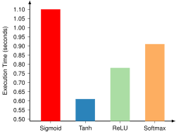](https://mlsysbook.ai/contents/core/training/dd9ebdd67961d212dfc551766d75c7c3bac5d682.svg "Figure 2: Activation Function Performance: CPU execution time varies significantly across common activation functions, with tanh and relu offering substantial speed advantages over sigmoid on this architecture. These differences impact system-level considerations such as training time and real-time inference capabilities, guiding activation function selection for performance-critical applications.")
Figure 2: **Activation Function Performance**: CPU execution time varies significantly across common activation functions, with tanh and relu offering substantial speed advantages over sigmoid on this architecture. These differences impact system-level considerations such as training time and real-time inference capabilities, guiding activation function selection for performance-critical applications.
While these benchmark results provide valuable insights, they represent CPU-only performance without hardware acceleration. In production environments, modern hardware accelerators like GPUs can substantially alter the relative performance characteristics of activation functions. System architects must therefore consider their specific hardware environment and deployment context when evaluating computational efficiency.
Recall from **[Chapter 3: Deep Learning Primer](https://mlsysbook.ai/contents/core/dl_primer/dl_primer.html#sec-dl-primer)
** that each activation function exhibits different gradient behavior, sparsity characteristics, and computational complexity. The question now is: how do these mathematical properties translate into hardware constraints and system performance? The following subsections examine each function’s implementation characteristics, focusing on software versus hardware trade-offs that determine real-world training efficiency:
###### Sigmoid
Sigmoid’s smooth \\((0,1)\\) bounded output makes it useful for probabilistic interpretation, but its vanishing gradient problem and non-zero-centered outputs present optimization challenges. From a systems perspective, the exponential function computation becomes the critical bottleneck. In software, this computation is expensive and inefficient[15](https://mlsysbook.ai/contents/core/training/training.html#fn15)
, particularly for deep networks or large datasets where millions of sigmoid evaluations occur per forward pass.
15 **Sigmoid Computational Cost**: Computing sigmoid requires expensive exponential operations. On CPU, `exp()` takes 10-20 clock cycles vs. 1 cycle for basic arithmetic. GPU implementations use 32-entry lookup tables with linear interpolation, reducing cost to 3-4 cycles but still 3x slower than ReLU. This overhead compounds in deep networks with millions of activations per forward pass.
These computational challenges are addressed differently in hardware. Modern accelerators like GPUs and TPUs typically avoid direct computation of the exponential function, instead using lookup tables (LUTs) or piece-wise linear approximations to balance accuracy with speed. While these hardware optimizations help, the multiple memory lookups and interpolation calculations still make sigmoid more resource-intensive than simpler functions like ReLU, even on highly parallel architectures.
###### Tanh
While tanh improves upon sigmoid with its \\((-1,1)\\) zero-centered outputs, it shares sigmoid’s computational burden. The exponential computations required for tanh create similar performance bottlenecks in both software and hardware implementations. In software, this computational overhead can slow training, particularly when working with large datasets or deep models.
In hardware, tanh uses its mathematical relationship with sigmoid (a scaled and shifted version) to optimize implementation. Modern hardware often implements tanh using a hybrid approach: lookup tables for common input ranges combined with piece-wise approximations for edge cases. This approach helps balance accuracy with computational efficiency, though tanh remains more resource-intensive than simpler functions. Despite these challenges, tanh remains common in RNNs and LSTMs[16](https://mlsysbook.ai/contents/core/training/training.html#fn16)
where balanced gradients are necessary.
16 **RNNs and LSTMs**: Long Short-Term Memory networks are specialized RNN variants designed to handle long-range dependencies. Both architectures are detailed in **[Chapter 4: DNN Architectures](https://mlsysbook.ai/contents/core/dnn_architectures/dnn_architectures.html#sec-dnn-architectures)
**.
###### ReLU
ReLU represents a shift in activation function design. Its mathematical simplicity—\\(\\max(0,x)\\)—avoids vanishing gradients and introduces beneficial sparsity, though it can suffer from dying neurons. This straightforward form has profound implications for system performance. In software, ReLU’s simple thresholding operation results in dramatically faster computation compared to sigmoid or tanh, requiring only a single comparison rather than exponential calculations.
The hardware implementation of ReLU showcases why it has become the dominant activation function in modern neural networks. Its simple \\(\\max(0,x)\\) operation requires just a single comparison and conditional set, translating to minimal circuit complexity[17](https://mlsysbook.ai/contents/core/training/training.html#fn17)
. Modern GPUs and TPUs can implement ReLU using a simple multiplexer that checks the input’s sign bit, allowing for extremely efficient parallel processing. This hardware efficiency, combined with the sparsity it introduces, results in both reduced computation time and lower memory bandwidth requirements.
17 **ReLU Hardware Efficiency**: ReLU requires just 1 instruction (`max(0,x)`) vs. sigmoid’s 10+ operations including exponentials. On NVIDIA GPUs, ReLU runs at 95% of peak FLOPS while sigmoid achieves only 30-40%. ReLU’s sparsity (typically 50% zeros) enables additional optimizations: sparse matrix operations, reduced memory bandwidth, and compressed gradients during backpropagation.
###### Softmax
Softmax differs from the element-wise functions above. Rather than processing inputs independently, softmax converts logits into probability distributions through global normalization, creating unique computational challenges. Its computation involves exponentiating each input value and normalizing by their sum, a process that becomes increasingly complex with larger output spaces. In software, this creates significant computational overhead for tasks like natural language processing, where vocabulary sizes can reach hundreds of thousands of terms. The function also requires keeping all values in memory during computation, as each output probability depends on the entire input vector.
At the hardware level, softmax faces unique challenges because it can’t process each value independently like other activation functions. Unlike ReLU’s simple threshold or even sigmoid’s per-value computation, softmax needs access to all values to perform normalization. This becomes particularly demanding in modern transformer architectures[18](https://mlsysbook.ai/contents/core/training/training.html#fn18)
, where softmax computations in attention mechanisms process thousands of values simultaneously. To manage these demands, hardware implementations often use approximation techniques or simplified versions of softmax, especially when dealing with large vocabularies or attention mechanisms.
18 **Transformer Attention**: The attention mechanism in transformers computes weighted relationships between all positions in a sequence simultaneously. This architecture is covered in **[Chapter 4: DNN Architectures](https://mlsysbook.ai/contents/core/dnn_architectures/dnn_architectures.html#sec-dnn-architectures)
**.
[Table 2](https://mlsysbook.ai/contents/core/training/training.html#tbl-compare-activations)
summarizes the trade-offs of these commonly used activation functions and highlights how these choices affect system performance.
Table 2: **Activation Function Trade-Offs**: Comparing activation functions exposes inherent advantages and disadvantages impacting system performance; for example, softmax’s normalization requirement poses hardware challenges in large-scale transformer models, while relu offers computational efficiency but can suffer from dying neurons. This table clarifies how activation function choices influence both model behavior and the practical constraints of machine learning system design.
| | | | |
| --- | --- | --- | --- |
| **Sigmoid** | Smooth gradients; bounded output in \\((0, 1)\\). | Vanishing gradients; non-zero-centered output. | Exponential computation adds overhead; limited scalability for deep networks on modern accelerators. |
| **Tanh** | Zero-centered output in \\((-1, 1)\\); stabilizes gradients. | Vanishing gradients for large inputs. | More expensive than ReLU; still commonly used in RNNs/LSTMs but less common in CNNs and Transformers. |
| **ReLU** | Computationally efficient; avoids vanishing gradients; introduces sparsity. | Dying neurons; unbounded output. | Simple operations optimize well on GPUs/TPUs; sparse activations reduce memory and computation needs. |
| **Softmax** | Converts logits into probabilities; sums to \\(1\\). | Computationally expensive for large outputs. | High cost for large vocabularies; hierarchical or sampled softmax needed for scalability in NLP tasks. |
The choice of activation function should balance computational considerations with their mathematical properties, such as handling vanishing gradients or introducing sparsity in neural activations. This data emphasizes the importance of evaluating both theoretical and practical performance when designing neural networks. For large-scale networks or real-time applications, ReLU is often the best choice due to its efficiency and scalability. However, for tasks requiring probabilistic outputs, such as classification, softmax remains indispensable despite its computational cost. Ultimately, the ideal activation function depends on the specific task, network architecture, and hardware environment.
GPT-2 GELU Activation Function
While the table above covers classical activation functions, GPT-2 uses the Gaussian Error Linear Unit (GELU), defined as: \\\[ \\text{GELU}(x) = x \\cdot \\Phi(x) = x \\cdot \\frac{1}{2}\\left\[1 + \\text{erf}\\left(\\frac{x}{\\sqrt{2}}\\right)\\right\] \\\]
where \\(\\Phi(x)\\) is the cumulative distribution function of the standard normal distribution.
**Why GELU for GPT-2?**
* Smoother gradients than ReLU, reducing the dying neuron problem
* Stochastic regularization effect: acts like dropout by probabilistically dropping inputs
* Better empirical performance on language modeling tasks
**System Performance Tradeoff**
* Computational cost: ~3 to 4x more expensive than ReLU (requires erf function evaluation)
* Memory: Same as ReLU (element-wise operation)
* Training time impact: For GPT-2’s 48 layers, GELU adds ~5 to 8% to total forward pass time
* Worth it: The improved model quality (lower perplexity) offsets the computational overhead
**Fast Approximation:** Modern frameworks (PyTorch, TensorFlow) implement GELU with optimized approximations:
# Fast GELU approximation (used in practice)
GELU(x) ≈ 0.5 * x * (1 + tanh(sqrt(2/π) * (x + 0.044715 * x³)))
This approximation reduces computational cost to ~1.5x ReLU while maintaining GELU’s benefits, demonstrating how production systems balance mathematical properties with implementation efficiency.
Systems Implication: Memory Bandwidth Bottlenecks
Activation functions reveal a critical systems principle: not all operations are compute-bound. While matrix multiplications saturate GPU compute units, activation functions often become **memory-bandwidth-bound**:
* **Low arithmetic intensity**: Element-wise operations perform few calculations per memory access (ReLU: 1 operation per load)
* **Limited parallelism benefit**: Simple operations complete faster than memory transfer time
* **Bandwidth constraints**: Modern GPUs have 10-100× more compute throughput than memory bandwidth
This explains why activation function choice matters less than expected—ReLU vs sigmoid shows only 2-3× difference despite vastly different computational complexity, because both are bottlenecked by memory access. The forward pass must carefully manage activation storage to prevent memory bandwidth from limiting overall training throughput.
### Optimization Algorithms
Optimization algorithms play an important role in neural network training by guiding the adjustment of model parameters to minimize a loss function. This process enables neural networks to learn from data, and it involves finding the optimal set of parameters that yield the best model performance on a given task. Broadly, these algorithms can be divided into two categories: classical methods, which provide the theoretical foundation, and advanced methods, which introduce enhancements for improved performance and efficiency.
These algorithms explore the complex, high-dimensional loss function surface, identifying regions where the function achieves its lowest values. This task is challenging because the loss function surface is rarely smooth or simple, often characterized by local minima, saddle points, and sharp gradients. Effective optimization algorithms are designed to overcome these challenges, ensuring convergence to a solution that generalizes well to unseen data. While this section covers optimization algorithms used during training, advanced optimization techniques including quantization, pruning, and knowledge distillation are detailed in **[Chapter 10: Model Optimizations](https://mlsysbook.ai/contents/core/optimizations/optimizations.html#sec-model-optimizations)
**.
The selection and design of optimization algorithms have significant system-level implications, such as computation efficiency, memory requirements, and scalability to large datasets or models. Systematic approaches to hyperparameter optimization, including grid search, Bayesian optimization, and automated machine learning workflows, are covered in **[Chapter 5: AI Workflow](https://mlsysbook.ai/contents/core/workflow/workflow.html#sec-ai-workflow)
**. A deeper understanding of these algorithms is essential for addressing the trade-offs between accuracy, speed, and resource usage.
#### Gradient-Based Optimization Methods
Modern neural network training relies on variations of gradient descent for parameter optimization. These approaches differ in how they process training data, leading to distinct system-level implications.
##### Gradient Descent
Gradient descent is the mathematical foundation of neural network training, iteratively adjusting parameters to minimize a loss function. The basic gradient descent algorithm computes the gradient of the loss with respect to each parameter, then updates parameters in the opposite direction of the gradient: \\\[ \\theta\_{t+1} = \\theta\_t - \\alpha \\nabla L(\\theta\_t) \\\]
The effectiveness of gradient descent in training systems reveals deep questions in optimization theory. Unlike convex optimization where gradient descent guarantees finding the global minimum, neural network loss surfaces contain exponentially many local minima. Yet gradient descent consistently finds solutions that generalize well, suggesting the optimization process has implicit biases toward solutions with desirable properties. Modern overparameterized networks, with more parameters than training examples, paradoxically achieve better generalization than smaller models, challenging traditional optimization intuitions.
In training systems, this mathematical operation translates into specific computational patterns. For each iteration, the system must:
1. Compute forward pass activations
2. Calculate loss value
3. Compute gradients through backpropagation
4. Update parameters using the gradient values
The computational demands of gradient descent scale with both model size and dataset size. Consider a neural network with \\(M\\) parameters training on \\(N\\) examples. Computing gradients requires storing intermediate activations during the forward pass for use in backpropagation. These activations consume memory proportional to the depth of the network and the number of examples being processed.
Traditional gradient descent processes the entire dataset in each iteration. For a training set with 1 million examples, computing gradients requires evaluating and storing results for each example before performing a parameter update. This approach poses significant system challenges: \\\[ \\text{Memory Required} = N \\times \\text{(Activation Memory + Gradient Memory)} \\\]
The memory requirements often exceed available hardware resources on modern hardware. A ResNet-50 model processing ImageNet-scale datasets would require hundreds of gigabytes of memory using this approach. Processing the full dataset before each update creates long iteration times, reducing the rate at which the model can learn from the data.
###### Stochastic Gradient Descent
These system constraints led to the development of variants that better align with hardware capabilities. The key insight was that exact gradient computation, while mathematically appealing, is not necessary for effective learning. This realization opened the door to methods that trade gradient accuracy for improved system efficiency.
These system limitations motivated the development of more efficient optimization approaches. SGD[19](https://mlsysbook.ai/contents/core/training/training.html#fn19)
is a big shift in the optimization strategy. Rather than computing gradients over the entire dataset, SGD estimates gradients using individual training examples: \\\[ \\theta\_{t+1} = \\theta\_t - \\alpha \\nabla L(\\theta\_t; x\_i, y\_i) \\\] where \\((x\_i, y\_i)\\) represents a single training example. This approach drastically reduces memory requirements since only one example’s activations and gradients need storage at any time.
19 **Stochastic Gradient Descent**: Originally developed by Robbins and Monro in 1951 for statistical optimization, SGD was first applied to neural networks by Rosenblatt for the perceptron in 1958. The method remained largely theoretical until the 1980s when computational constraints made full-batch gradient descent impractical for larger networks. Today’s “mini-batch SGD” (processing 32-512 examples) represents a compromise between the original single-example approach and full-batch methods, enabling parallel processing on modern GPUs. The stochastic nature of these updates introduces noise into the optimization process, but this noise often helps escape local minima and reach better solutions.
However, processing single examples creates new system challenges. Modern accelerators achieve peak performance through parallel computation, processing multiple data elements simultaneously. Single-example updates leave most computing resources idle, resulting in poor hardware utilization. The frequent parameter updates also increase memory bandwidth requirements, as weights must be read and written for each example rather than amortizing these operations across multiple examples.
##### Mini-batch Processing
**Definition:** Batch Processing
**_Batch Processing_** is the technique of computing gradients over _groups of training examples_ simultaneously, enabling efficient _parallel computation_ and improved _hardware utilization_ during model training.
Mini-batch gradient descent emerges as a practical compromise between full-batch and stochastic methods. It computes gradients over small batches of examples, enabling parallel computations that align well with modern GPU architectures ([Dean and Ghemawat 2008](https://mlsysbook.ai/contents/core/training/training.html#ref-dean2012large)
). \\\[ \\theta\_{t+1} = \\theta\_t - \\alpha \\frac{1}{B} \\sum\_{i=1}^B \\nabla L(\\theta\_t; x\_i, y\_i) \\\]
Dean, Jeffrey, and Sanjay Ghemawat. 2008. “MapReduce: Simplified Data Processing on Large Clusters.” _Communications of the ACM_ 51 (1): 107–13. [https://doi.org/10.1145/1327452.1327492](https://doi.org/10.1145/1327452.1327492)
.
Mini-batch processing aligns well with modern hardware capabilities. Consider a training system using GPU hardware. These devices contain thousands of cores designed for parallel computation. Mini-batch processing allows these cores to simultaneously compute gradients for multiple examples, improving hardware utilization. The batch size B becomes a key system parameter, influencing both computational efficiency and memory requirements.
The relationship between batch size and system performance follows clear patterns that reveal hardware-software trade-offs. Memory requirements scale linearly with batch size, but the specific costs vary dramatically by model architecture: \\\[ \\begin{aligned} \\text{Memory Required} = B \\times (&\\text{Activation Memory} \\\\ &+ \\text{Gradient Memory} \\\\ &+ \\text{Parameter Memory}) \\end{aligned} \\\]
For concrete understanding, consider ResNet-50 training with different batch sizes. At batch size 32, the model requires approximately 8GB of activation memory, 4GB for gradients, and 200MB for parameters per GPU. Doubling to batch size 64 doubles these memory requirements to 16GB activations and 8GB gradients. This linear scaling quickly exhausts GPU memory, with high-end training GPUs typically providing 40-80GB of HBM.
Larger batches enable more efficient computation through improved parallelism and better memory access patterns. GPU utilization efficiency demonstrates this trade-off: batch sizes of 256 or higher typically achieve over 90% hardware utilization on modern training accelerators, while smaller batches of 16-32 may only achieve 60-70% utilization due to insufficient parallelism to saturate the hardware.
This establishes a central theme in training systems: the hardware-software trade-off between memory constraints and computational efficiency. Training systems must select batch sizes that maximize hardware utilization while fitting within available memory. The optimal choice often requires gradient accumulation when memory constraints prevent using efficiently large batches, trading increased computation for the same effective batch size.
#### Adaptive and Momentum-Based Optimizers
Advanced optimization algorithms introduce mechanisms like momentum and adaptive learning rates to improve convergence. These methods have been instrumental in addressing the inefficiencies of classical approaches ([Kingma and Ba 2014](https://mlsysbook.ai/contents/core/training/training.html#ref-kingma2014adam)
).
Kingma, Diederik P., and Jimmy Ba. 2014. “Adam: A Method for Stochastic Optimization.” _ICLR_, December. [http://arxiv.org/abs/1412.6980v9](http://arxiv.org/abs/1412.6980v9)
.
##### Momentum-Based Methods
Momentum methods enhance gradient descent by accumulating a velocity vector across iterations. The momentum update equations introduce an additional term to track the history of parameter updates: \\\[\\begin{gather\*} v\_{t+1} = \\beta v\_t + \\nabla L(\\theta\_t) \\\\ \\theta\_{t+1} = \\theta\_t - \\alpha v\_{t+1} \\end{gather\*}\\\] where \\(\\beta\\) is the momentum coefficient, typically set between 0.9 and 0.99. From a systems perspective, momentum introduces additional memory requirements. The training system must maintain a velocity vector with the same dimensionality as the parameter vector, effectively doubling the memory needed for optimization state.
##### Adaptive Learning Rate Methods
RMSprop modifies the basic gradient descent update by maintaining a moving average of squared gradients for each parameter: \\\[\\begin{gather\*} s\_t = \\gamma s\_{t-1} + (1-\\gamma)\\big(\\nabla L(\\theta\_t)\\big)^2 \\\\ \\theta\_{t+1} = \\theta\_t - \\alpha \\frac{\\nabla L(\\theta\_t)}{\\sqrt{s\_t + \\epsilon}} \\end{gather\*}\\\]
This per-parameter adaptation requires storing the moving average \\(s\_t\\), creating memory overhead similar to momentum methods. The element-wise operations in RMSprop also introduce additional computational steps compared to basic gradient descent.
##### Adam Optimization
Adam combines concepts from both momentum and RMSprop, maintaining two moving averages for each parameter: \\\[\\begin{gather\*} m\_t = \\beta\_1 m\_{t-1} + (1-\\beta\_1)\\nabla L(\\theta\_t) \\\\ v\_t = \\beta\_2 v\_{t-1} + (1-\\beta\_2)\\big(\\nabla L(\\theta\_t)\\big)^2 \\\\ \\theta\_{t+1} = \\theta\_t - \\alpha \\frac{m\_t}{\\sqrt{v\_t + \\epsilon}} \\end{gather\*}\\\]
The system implications of Adam are more substantial than previous methods. The optimizer must store two additional vectors (\\(m\_t\\) and \\(v\_t\\)) for each parameter, tripling the memory required for optimization state. For a model with 100 million parameters using 32-bit floating-point numbers, the additional memory requirement is approximately 800 MB.
#### Optimization Algorithm System Implications
The practical implementation of both classical and advanced optimization methods requires careful consideration of system resources and hardware capabilities. Understanding these implications helps inform algorithm selection and system design choices.
##### Optimization Trade-offs
The choice of optimization algorithm creates specific patterns of computation and memory access that influence training efficiency. Memory requirements increase progressively from basic gradient descent to more sophisticated methods: \\\[\\begin{gather\*} \\text{Memory}\_{\\text{SGD}} = \\text{Size}\_{\\text{params}} \\\\ \\text{Memory}\_{\\text{Momentum}} = 2 \\times \\text{Size}\_{\\text{params}} \\\\ \\text{Memory}\_{\\text{Adam}} = 3 \\times \\text{Size}\_{\\text{params}} \\end{gather\*}\\\]
These memory costs must be balanced against convergence benefits. While Adam often requires fewer iterations to reach convergence, its per-iteration memory and computation overhead may impact training speed on memory-constrained systems.
GPT-2 Adam Optimizer Memory Requirements
GPT-2 training uses the Adam optimizer with these hyperparameters:
* β₁ = 0.9 (momentum decay)
* β₂ = 0.999 (second moment decay)
* Learning rate: Warmed up from 0 to 2.5e-4 over first 500 steps, then cosine decay
* Weight decay: 0.01
* Gradient clipping: Global norm clipping at 1.0
**Memory Overhead Calculation**
For GPT-2’s 1.5B parameters in FP32 (4 bytes each):
* Parameters: 1.5B × 4 bytes = 6.0 GB
* Gradients: 1.5B × 4 bytes = 6.0 GB
* Adam first moment (m): 1.5B × 4 bytes = 6.0 GB
* Adam second moment (v): 1.5B × 4 bytes = 6.0 GB
* Total optimizer state: 24 GB
This explains why GPT-2 training requires 32GB+ V100 GPUs even before considering activation memory.
**System Decisions Driven by Optimizer**
1. Mixed precision training (FP16 params, FP32 optimizer state) cuts this to ~15GB
2. Gradient accumulation (splitting effective batches into smaller micro-batches, accumulating gradients across multiple forward/backward passes before updating, detailed in [Section 1.5.5](https://mlsysbook.ai/contents/core/training/training.html#sec-ai-training-gradient-accumulation-checkpointing-26ab)
) allows effective batch\_size=512 despite memory limits
3. Optimizer state sharding (ZeRO-2) distributes Adam state across GPUs in distributed training
**Convergence Tradeoff:** Adam’s memory overhead is worth it. GPT-2 converges in ~50K steps vs. ~150K+ steps with SGD+Momentum, saving weeks of training time despite higher per-step cost.
##### Implementation Considerations
The efficient implementation of optimization algorithms in training frameworks hinges on strategic system-level considerations that directly influence performance. Key factors include memory bandwidth management, operation fusion techniques, and numerical precision optimization. These elements collectively determine the computational efficiency, memory utilization, and scalability of optimizers across diverse hardware architectures.
Memory bandwidth presents the primary bottleneck in optimizer implementation. Modern frameworks address this through operation fusion, which reduces memory access overhead by combining multiple operations into a single kernel. For example, the Adam optimizer’s memory access requirements can grow linearly with parameter size when operations are performed separately: \\\[ \\text{Bandwidth}\_{\\text{separate}} = 5 \\times \\text{Size}\_{\\text{params}} \\\]
However, fusing these operations into a single computational kernel significantly reduces the bandwidth requirement: \\\[ \\text{Bandwidth}\_{\\text{fused}} = 2 \\times \\text{Size}\_{\\text{params}} \\\]
These techniques have been effectively demonstrated in systems like cuDNN and other GPU-accelerated frameworks that optimize memory bandwidth usage and operation fusion ([Chetlur et al. 2014](https://mlsysbook.ai/contents/core/training/training.html#ref-chetlur2014cudnn)
; [Jouppi et al. 2017](https://mlsysbook.ai/contents/core/training/training.html#ref-jouppi2017tpu)
).
Chetlur, Sharan, Cliff Woolley, Philippe Vandermersch, Jonathan Cohen, John Tran, Bryan Catanzaro, and Evan Shelhamer. 2014. “cuDNN: Efficient Primitives for Deep Learning.” _arXiv Preprint arXiv:1410.0759_, October. [http://arxiv.org/abs/1410.0759v3](http://arxiv.org/abs/1410.0759v3)
.
Memory access patterns also play an important role in determining the efficiency of cache utilization. Sequential access to parameter and optimizer state vectors maximizes cache hit rates and effective memory bandwidth. This principle is evident in hardware such as GPUs and tensor processing units (TPUs), where optimized memory layouts significantly improve performance ([Jouppi et al. 2017](https://mlsysbook.ai/contents/core/training/training.html#ref-jouppi2017tpu)
).
Numerical precision represents another important tradeoff in implementation. Empirical studies have shown that optimizer states remain stable even when reduced precision formats, such as 16-bit floating-point (FP16), are used. Transitioning from 32-bit to 16-bit formats reduces memory requirements, as illustrated for the Adam optimizer: \\\[ \\text{Memory}\_{\\text{Adam-FP16}} = \\frac{3}{2} \\times \\text{Size}\_{\\text{params}} \\\]
Mixed-precision training[20](https://mlsysbook.ai/contents/core/training/training.html#fn20)
has been shown to achieve comparable accuracy while significantly reducing memory consumption and computational overhead ([Micikevicius et al. 2017](https://mlsysbook.ai/contents/core/training/training.html#ref-micikevicius2017mixed)
; [Krishnamoorthi 2018](https://mlsysbook.ai/contents/core/training/training.html#ref-krishnamoorthi2018quantizing)
).
20 **Mixed-Precision Training**: Introduced by NVIDIA in 2018, this technique uses FP16 for forward/backward passes while maintaining FP32 precision for loss scaling, enabling 2x memory savings and 1.6x speedups on Tensor Core GPUs while maintaining model accuracy.
Krishnamoorthi, Raghuraman. 2018. “Quantizing Deep Convolutional Networks for Efficient Inference: A Whitepaper.” _arXiv Preprint arXiv:1806.08342_, June. [http://arxiv.org/abs/1806.08342v1](http://arxiv.org/abs/1806.08342v1)
.
Chen, Tianqi, Mu Li, Yutian Li, Min Lin, Naiyan Wang, Minjie Wang, Tianjun Xiao, Bing Xu, Chiyuan Zhang, and Zheng Zhang. 2015. “MXNet: A Flexible and Efficient Machine Learning Library for Heterogeneous Distributed Systems.” _arXiv Preprint arXiv:1512.01274_, December. [http://arxiv.org/abs/1512.01274v1](http://arxiv.org/abs/1512.01274v1)
.
The above implementation factors determine the practical performance of optimization algorithms in deep learning systems, emphasizing the importance of tailoring memory, computational, and numerical strategies to the underlying hardware architecture ([T. Chen et al. 2015](https://mlsysbook.ai/contents/core/training/training.html#ref-chen2015mxnet)
).
##### Optimizer Trade-offs
The evolution of optimization algorithms in neural network training reveals an intersection between algorithmic efficiency and system performance. While optimizers were primarily developed to improve model convergence, their implementation significantly impacts memory usage, computational requirements, and hardware utilization.
A deeper examination of popular optimization algorithms reveals their varying impacts on system resources. As shown in [Table 3](https://mlsysbook.ai/contents/core/training/training.html#tbl-optimizer-properties)
, each optimizer presents distinct trade-offs between memory usage, computational patterns, and convergence behavior. SGD maintains minimal memory overhead, requiring storage only for model parameters and current gradients. This lightweight memory footprint comes at the cost of slower convergence and potentially poor hardware utilization due to its sequential update nature.
Table 3: **Optimizer Memory Footprint**: Different optimization algorithms impose varying memory costs due to the storage of intermediate values like gradients, velocities, and squared gradients; understanding these trade-offs is important for resource-constrained deployments and large-scale model training. Selecting an optimizer involves balancing convergence speed with available memory and computational resources.
| | | | | |
| --- | --- | --- | --- | --- |
| **Memory Overhead** | None | Velocity terms | Squared gradients | Both velocity and squared gradients |
| **Memory Cost** | \\(1\\times\\) | \\(2\\times\\) | \\(2\\times\\) | \\(3\\times\\) |
| **Access Pattern** | Sequential | Sequential | Random | Random |
| **Operations/Parameter** | 2 | 3 | 4 | 5 |
| **Hardware Efficiency** | Low | Medium | High | Highest |
| **Convergence Speed** | Slowest | Medium | Fast | Fastest |
Momentum methods introduce additional memory requirements by storing velocity terms for each parameter, doubling the memory footprint compared to SGD. This increased memory cost brings improved convergence through better gradient estimation, while maintaining relatively efficient memory access patterns. The sequential nature of momentum updates allows for effective hardware prefetching and cache utilization.
RMSprop adapts learning rates per parameter by tracking squared gradient statistics. Its memory overhead matches momentum methods, but its computation patterns become more irregular. The algorithm requires additional arithmetic operations for maintaining running averages and computing adaptive learning rates, increasing computational intensity from 3 to 4 operations per parameter.
Adam combines the benefits of momentum and adaptive learning rates, but at the highest system resource cost. [Table 3](https://mlsysbook.ai/contents/core/training/training.html#tbl-optimizer-properties)
reveals that it maintains both velocity terms and squared gradient statistics, tripling the memory requirements compared to SGD. The algorithm’s computational patterns involve 5 operations per parameter update, though these operations often utilize hardware more effectively due to their regular structure and potential for parallelization.
Training system designers must balance these trade-offs when selecting optimization strategies. Modern hardware architectures influence these decisions. GPUs excel at the parallel computations required by adaptive methods, while memory-constrained systems might favor simpler optimizers. The choice of optimizer affects not only training dynamics but also maximum feasible model size, achievable batch size, hardware utilization efficiency, and overall training time to convergence. Beyond optimizer selection, learning rate scheduling strategies, including cosine annealing, linear warmup, and cyclical schedules, further influence convergence behavior and final model performance, with large-batch training requiring careful scaling adjustments as detailed in distributed training discussions.
Modern training frameworks continue to evolve, developing techniques like optimizer state sharding, mixed-precision storage, and fused operations to better balance these competing demands. Understanding these system implications helps practitioners make informed decisions about optimization strategies based on their specific hardware constraints and training requirements.
#### Framework Optimizer Interface
While the mathematical formulations of SGD, momentum, and Adam establish the theoretical foundations for parameter optimization, frameworks provide standardized interfaces that abstract these algorithms into practical training loops. Understanding how frameworks like PyTorch implement optimizer APIs demonstrates how complex mathematical operations become accessible through clean abstractions.
The framework optimizer interface follows a consistent pattern that separates gradient computation from parameter updates. This separation enables the mathematical algorithms to be applied systematically across diverse model architectures and training scenarios.
Framework optimizers implement a four-step training cycle that encapsulates the mathematical operations within a clean API. The following example demonstrates how Adam optimization integrates into a standard training loop:
import torch
import torch.nn as nn
import torch.optim as optim
# Initialize Adam optimizer with model parameters
# and learning rate
optimizer = optim.Adam(
model.parameters(), lr=0.001, betas=(0.9, 0.999)
)
loss_function = nn.CrossEntropyLoss()
# Standard training loop implementing the four-step optimization cycle
for epoch in range(num_epochs):
for batch_idx, (data, targets) in enumerate(dataloader):
# Step 1: Clear accumulated gradients from previous iteration
optimizer.zero_grad()
# Step 2: Forward pass - compute model predictions
predictions = model(data)
loss = loss_function(predictions, targets)
# Step 3: Backward pass - compute gradients via
# automatic differentiation
loss.backward()
# Step 4: Parameter update - apply Adam optimization equations
optimizer.step()
The `optimizer.zero_grad()` call addresses a critical framework implementation detail: gradients accumulate across calls to `backward()`, requiring explicit clearing between batches. This behavior enables gradient accumulation patterns for large effective batch sizes but requires careful management in standard training loops.
The `optimizer.step()` method encapsulates the mathematical update equations. For Adam optimization, this single call implements the momentum estimation, squared gradient tracking, bias correction, and parameter update computation automatically. The following code illustrates the mathematical operations that occur within the optimizer:
# Mathematical operations implemented by optimizer.step() for Adam
# These computations happen automatically within the framework
# Adam hyperparameters (typically β₁=0.9, β₂=0.999, ε=1e-8)
beta_1, beta_2, epsilon = 0.9, 0.999, 1e-8
learning_rate = 0.001
# For each parameter tensor in the model:
for param in model.parameters():
if param.grad is not None:
grad = param.grad.data # Current gradient
# Step 1: Update biased first moment estimate
# (momentum)
# m_t = β₁ * m_{t-1} + (1-β₁) * ∇L(θₜ)
momentum_buffer = (
beta_1 * momentum_buffer + (1 - beta_1) * grad
)
# Step 2: Update biased second moment estimate
# (squared gradients)
# v_t = β₂ * v_{t-1} + (1-β₂) * (∇L(θₜ))²
variance_buffer = beta_2 * variance_buffer + (
1 - beta_2
) * grad.pow(2)
# Step 3: Compute bias-corrected estimates
momentum_corrected = momentum_buffer / (
1 - beta_1**step_count
)
variance_corrected = variance_buffer / (
1 - beta_2**step_count
)
# Step 4: Apply parameter update
# θ_{t+1} = θₜ - α * m_t / (√v_t + ε)
param.data -= (
learning_rate
* momentum_corrected
/ (variance_corrected.sqrt() + epsilon)
)
Framework implementations also handle the memory management challenges in optimizer trade-offs. The optimizer automatically allocates storage for momentum terms and squared gradient statistics, managing the 2-3x memory overhead transparently while providing efficient memory access patterns optimized for the underlying hardware.
##### Learning Rate Scheduling Integration
Frameworks integrate learning rate scheduling directly into the optimizer interface, enabling dynamic adjustment of the learning rate α during training. This integration demonstrates how frameworks compose multiple optimization techniques through modular design patterns.
Learning rate schedulers modify the optimizer’s learning rate according to predefined schedules, such as cosine annealing, exponential decay, or step-wise reductions. The following example demonstrates how to integrate cosine annealing with Adam optimization:
import torch
import torch.optim as optim
import torch.optim.lr_scheduler as lr_scheduler
import math
# Initialize optimizer with initial learning rate
optimizer = optim.Adam(
model.parameters(), lr=0.001, weight_decay=1e-4
)
# Configure cosine annealing scheduler
# T_max: number of epochs for one complete cosine cycle
# eta_min: minimum learning rate (default: 0)
scheduler = lr_scheduler.CosineAnnealingLR(
optimizer,
T_max=100, # Complete cycle over 100 epochs
eta_min=1e-6, # Minimum learning rate
)
# Training loop with integrated learning rate scheduling
for epoch in range(num_epochs):
# Track learning rate for monitoring
current_lr = optimizer.param_groups[0]["lr"]
print(f"Epoch {epoch}: Learning Rate = {current_lr:.6f}")
# Standard training loop
for batch_idx, (data, targets) in enumerate(dataloader):
optimizer.zero_grad()
predictions = model(data)
loss = loss_function(predictions, targets)
loss.backward()
optimizer.step()
# Update learning rate at end of epoch
# Implements: lr = eta_min + (eta_max - eta_min) * (1 + cos(π * epoch / T_max)) / 2
scheduler.step()
This composition pattern allows practitioners to combine base optimization algorithms (SGD, Adam) with scheduling strategies (cosine annealing, linear warmup) without modifying the core mathematical implementations. The framework handles the coordination between components while maintaining the mathematical properties of each algorithm.
The optimizer interface exemplifies how frameworks balance mathematical rigor with practical usability. The underlying algorithms implement the precise mathematical formulations we studied, while the API design enables practitioners to focus on model architecture and training dynamics rather than optimization implementation details.
### Backpropagation Mechanics
The backpropagation algorithm[21](https://mlsysbook.ai/contents/core/training/training.html#fn21)
computes gradients by systematically moving backward through a neural network’s computational graph. While earlier discussions introduced backpropagation’s mathematical principles, implementing this algorithm in training systems requires careful management of memory, computation, and data flow.
21 **Backpropagation Algorithm**: Independently rediscovered multiple times, backpropagation was popularized by Rumelhart, Hinton, and Williams in 1986 (though similar ideas appeared in Werbos 1974). This breakthrough enabled training of deep networks by efficiently computing gradients in O(n) time vs. naive O(n²) approaches. Modern implementations require careful memory management since storing all activations for a ResNet-50 consumes 1.2GB per image.
#### Backpropagation Algorithm Mechanics
Neural networks learn by adjusting their parameters to reduce errors through the backpropagation algorithm, which computes how much each parameter contributed to the error by systematically moving backward through the network’s computational graph.
During the forward pass, each layer performs computations and produces activations that must be stored for the backward pass: \\\[\\begin{gather\*} z^{(l)} = W^{(l)}a^{(l-1)} + b^{(l)} \\\\ a^{(l)} = f(z^{(l)}) \\end{gather\*}\\\] where \\(z^{(l)}\\) represents the pre-activation values and \\(a^{(l)}\\) represents the activations at layer \\(l\\). The storage of these intermediate values creates specific memory requirements that scale with network depth and batch size.
The backward pass computes gradients by applying the chain rule, starting from the network’s output and moving toward the input: \\\[\\begin{gather\*} \\frac{\\partial L}{\\partial z^{(l)}}=\\frac{\\partial L}{\\partial a^{(l)}} \\odot f'(z^{(l)}) \\\\ \\frac{\\partial L}{\\partial W^{(l)}}=\\frac{\\partial L}{\\partial z^{(l)}}\\big(a^{(l-1)}\\big)^T \\end{gather\*}\\\]
For a network with parameters \\(W\_i\\) at each layer, computing \\(\\frac{\\partial L}{\\partial W\_i}\\) determines how much the loss L changes when adjusting each parameter. The chain rule provides a systematic way to organize these computations: \\\[ \\frac{\\partial L\_{full}}{\\partial L\_{i}} = \\frac{\\partial A\_{i}}{\\partial L\_{i}} \\frac{\\partial L\_{i+1}}{\\partial A\_{i}} ... \\frac{\\partial A\_{n}}{\\partial L\_{n}} \\frac{\\partial L\_{full}}{\\partial A\_{n}} \\\]
This equation reveals key requirements for training systems. Computing gradients for early layers requires information from all later layers, creating specific patterns in data storage and access. Each gradient computation requires access to stored activations from the forward pass, creating a specific pattern of memory access and computation that training systems must manage efficiently. These patterns directly influence the efficiency of optimization algorithms like SGD or Adam discussed earlier. Modern training systems use autodifferentiation[22](https://mlsysbook.ai/contents/core/training/training.html#fn22)
to handle these computations automatically, but the underlying system requirements remain the same.
22 **Automatic Differentiation**: Not to be confused with symbolic or numerical differentiation, autodiff constructs a computational graph at runtime and applies the chain rule systematically. PyTorch uses “define-by-run” (dynamic graphs built during forward pass) while TensorFlow v1 used static graphs. This enables complex architectures like RNNs and transformers where graph structure changes dynamically, but requires careful memory management since the entire forward computation graph must be preserved for the backward pass.
#### Activation Memory Requirements
Training systems must maintain intermediate values (activations) from the forward pass to compute gradients during the backward pass. This requirement compounds the memory demands of optimization algorithms. For each layer l, the system must store:
* Input activations from the forward pass
* Output activations after applying layer operations
* Layer parameters being optimized
* Computed gradients for parameter updates
Consider a batch of training examples passing through a network. The forward pass computes and stores: \\\[\\begin{gather\*} z^{(l)} = W^{(l)}a^{(l-1)} + b^{(l)} \\\\ a^{(l)} = f(z^{(l)}) \\end{gather\*}\\\]
Both \\(z^{(l)}\\) and \\(a^{(l)}\\) must be cached for the backward pass. This creates a multiplicative effect on memory usage: each layer’s memory requirement is multiplied by the batch size, and the optimizer’s memory overhead (discussed in the previous section) applies to each parameter.
The total memory needed scales with:
* Network depth (number of layers)
* Layer widths (number of parameters per layer)
* Batch size (number of examples processed together)
* Optimizer state (additional memory for algorithms like Adam)
This creates a complex set of trade-offs. Larger batch sizes enable more efficient computation and better gradient estimates for optimization, but require proportionally more memory for storing activations. More sophisticated optimizers like Adam can achieve faster convergence but require additional memory per parameter.
GPT-2 Activation Memory Breakdown
For GPT-2 with batch\_size=32, seq\_len=1024, hidden\_dim=1280, 48 layers:
**Per-Layer Activation Memory**
* Attention activations: `batch × seq × hidden × 4` (Q, K, V, output) = 32 × 1024 × 1280 × 4 × 2 bytes (FP16) = 335 MB
* FFN activations: `batch × seq × (hidden × 4)` (intermediate expansion) = 32 × 1024 × 5120 × 2 bytes = 335 MB
* Layer norm states: Minimal (~10 MB per layer)
* Total per layer: ~680 MB
**Full Model Activation Memory**
* 48 layers × 680 MB = **32.6 GB** just for activations
* Parameters (FP16): 3 GB
* Gradients: 3 GB
* Optimizer state (Adam, FP32): 12 GB
* Peak memory during training: **~51 GB**
This exceeds a single V100’s 32GB capacity.
**System Solutions Applied**
1. Gradient checkpointing: Recompute activations during backward pass, reducing activation memory by 75% (to ~8 GB) at cost of 33% more compute
2. Activation CPU offloading: Store some activations in CPU RAM, transfer during backward pass
3. Mixed precision: FP16 activations (already applied above) vs FP32 (would be 65 GB)
4. Reduced batch size: Use batch\_size=16 per GPU + gradient accumulation over 2 steps = effective batch\_size=32
**Training Configuration:** Most GPT-2 implementations use gradient checkpointing + batch\_size=16 per GPU, fitting comfortably in 32GB V100s while maintaining training efficiency.
#### Memory-Computation Trade-offs
Training systems must balance memory usage against computational efficiency. Each forward pass through the network generates a set of activations that must be stored for the backward pass. For a neural network with \\(L\\) layers, processing a batch of \\(B\\) examples requires storing: \\\[ \\text{Memory per batch} = B \\times \\sum\_{l=1}^L (s\_l + a\_l) \\\] where \\(s\_l\\) represents the size of intermediate computations (like \\(z^{(l)}\\)) and \\(a\_l\\) represents the activation outputs at layer l.
This memory requirement compounds with the optimizer’s memory needs discussed in the previous section. The total memory consumption of a training system includes both the stored activations and the optimizer state: \\\[ \\text{Total Memory} = \\text{Memory per batch} + \\text{Memory}\_{\\text{optimizer}} \\\]
To manage these substantial memory requirements, training systems use several sophisticated strategies. Gradient checkpointing is a basic approach, strategically recomputing some intermediate values during the backward pass rather than storing them. While this increases computational work, it can significantly reduce memory usage, enabling training of deeper networks or larger batch sizes on memory-constrained hardware ([T. Chen et al. 2016](https://mlsysbook.ai/contents/core/training/training.html#ref-chen2016training)
).
Chen, Tianqi, Bing Xu, Chiyuan Zhang, and Carlos Guestrin. 2016. “Training Deep Nets with Sublinear Memory Cost.” _CoRR_ abs/1604.06174 (April). [http://arxiv.org/abs/1604.06174v2](http://arxiv.org/abs/1604.06174v2)
.
The efficiency of these memory management strategies depends heavily on the underlying hardware architecture. GPU systems, with their high computational throughput but limited memory bandwidth, often encounter different bottlenecks than CPU systems. Memory bandwidth limitations on GPUs mean that even when sufficient storage exists, moving data between memory and compute units can become the primary performance constraint ([Jouppi et al. 2017](https://mlsysbook.ai/contents/core/training/training.html#ref-jouppi2017tpu)
).
These hardware considerations naturally guide the implementation of backpropagation in modern training systems. Responding to these constraints, specialized memory-efficient algorithms for operations like convolutions compute gradients in tiles or chunks, adapting to available memory bandwidth. Dynamic memory management tracks the lifetime of intermediate values throughout the computation graph, deallocating memory as soon as tensors become unnecessary for subsequent computations ([Paszke et al. 2019](https://mlsysbook.ai/contents/core/training/training.html#ref-paszke2019pytorch)
).
Paszke, Adam, Sam Gross, Francisco Massa, and et al. 2019. “PyTorch: An Imperative Style, High-Performance Deep Learning Library.” _Advances in Neural Information Processing Systems (NeurIPS)_ 32: 8026–37.
### Mathematical Foundations System Implications
The mathematical operations we have examined—forward propagation, gradient computation, and parameter updates—define what training systems must compute. Understanding these operations in mathematical terms provides essential knowledge, but implementing them in practical training systems requires translating mathematical abstractions into orchestrated computational workflows. This translation introduces distinct challenges centered on resource coordination, timing, and data movement.
Efficiently executing training requires coordinating these mathematical operations with data loading pipelines, preprocessing workflows, hardware accelerators, and monitoring systems. The matrix multiplications that dominate forward and backward passes must be scheduled to overlap with data transfer operations to prevent GPU idle time. Activation storage requirements from forward propagation influence batch size selection and memory allocation strategies. The sequential dependencies imposed by backpropagation constrain parallelization opportunities and shape distributed training architectures. These system-level considerations transform mathematical operations into concrete computational pipelines.
**Self-Check: Question 1.3**
1. Which of the following operations is most computationally dominant in neural network training?
1. Matrix-vector multiplication
2. Matrix-matrix multiplication
3. Element-wise activation functions
4. Batch normalization
2. Explain how the choice of activation function can impact system performance in neural network training.
3. Order the following steps in the backpropagation process: (1) Compute gradients, (2) Forward pass, (3) Update parameters.
4. What is a primary system-level challenge when using advanced optimization algorithms like Adam?
1. High computational intensity
2. Limited convergence speed
3. Increased memory overhead
4. Poor hardware utilization
5. Consider a scenario where you are designing a training system for a large neural network. What trade-offs would you consider when selecting an optimization algorithm?
[See Answers →](https://mlsysbook.ai/contents/core/training/training.html#quiz-answer-sec-ai-training-mathematical-foundations-71a8)
Pipeline Architecture
---------------------
The mathematical operations examined above define what training systems must compute. Pipeline architecture determines how to orchestrate these computations efficiently across real hardware with finite memory and bandwidth constraints. A training pipeline provides the organizational framework that coordinates mathematical operations with data movement, system resources, and operational monitoring. This architectural perspective enables optimization not just of individual operations, but their orchestration across the entire training process.
As shown in [Figure 3](https://mlsysbook.ai/contents/core/training/training.html#fig-training-pipeline)
, the training pipeline consists of three main components: the data pipeline for ingestion and preprocessing, the training loop that handles model updates, and the evaluation pipeline for assessing performance. These components work together in a coordinated manner, with processed batches flowing from the data pipeline to the training loop, and evaluation metrics providing feedback to guide the training process.
[](https://mlsysbook.ai/contents/core/training/a10a3b3d8979ed157f8a6b3d6845e87e7c9ca6f9.svg "Figure 3: Pipeline Architecture: Machine learning systems organize training through interconnected data, training, and evaluation pipelines, enabling iterative model refinement and performance assessment. Data flows sequentially through these components, with evaluation metrics providing feedback to optimize the training process and ensure reproducible results.")
Figure 3: **Pipeline Architecture**: Machine learning systems organize training through interconnected data, training, and evaluation pipelines, enabling iterative model refinement and performance assessment. Data flows sequentially through these components, with evaluation metrics providing feedback to optimize the training process and ensure reproducible results.
### Architectural Overview
To understand how these mathematical operations translate into practical systems, the architecture of a training pipeline is organized around three interconnected components: the data pipeline, the training loop, and the evaluation pipeline. These components collectively process raw data, train the model, and assess its performance, ensuring that the training process is efficient and effective.
This modular organization enables efficient resource utilization and clear separation of concerns. The data pipeline initiates the process by ingesting raw data and transforming it into a format suitable for the model. This data is passed to the training loop, where the model performs its core computations to learn from the inputs. Periodically, the evaluation pipeline assesses the model’s performance using a separate validation dataset. This modular structure ensures that each stage operates efficiently while contributing to the overall workflow.
#### Data Pipeline
Understanding each component’s role begins with the data pipeline, which manages the ingestion, preprocessing, and batching of data for training. Raw data is typically loaded from local storage and transformed dynamically during training to avoid redundancy and enhance diversity. For instance, image datasets may undergo preprocessing steps like normalization, resizing, and augmentation to improve the robustness of the model. These operations are performed in real time to minimize storage overhead and adapt to the specific requirements of the task ([LeCun et al. 1998](https://mlsysbook.ai/contents/core/training/training.html#ref-lecun1998efficient)
). Once processed, the data is packaged into batches and handed off to the training loop.
LeCun, Yann, Leon Bottou, Genevieve B. Orr, and Klaus -Robert Müller. 1998. “Efficient BackProp.” In _Neural Networks: Tricks of the Trade_, 1524:9–50. Springer Berlin Heidelberg. [https://doi.org/10.1007/3-540-49430-8\\\_2](https://doi.org/10.1007/3-540-49430-8/_2)
.
#### Training Loop
The training loop is the computational core of the pipeline, where the model learns from the prepared data. [Figure 4](https://mlsysbook.ai/contents/core/training/training.html#fig-training-loop)
illustrates this process, highlighting the forward pass, loss computation, and parameter updates on a single GPU:
[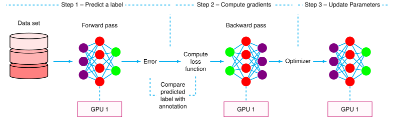](https://mlsysbook.ai/contents/core/training/768b8af793e9b0fefe5cb2ca2a4b8f2771220715.svg "Figure 4: GPU-Accelerated Training: Modern deep learning relies on gpus to parallelize matrix operations, significantly accelerating the forward and backward passes required for parameter updates during training. This single-GPU workflow iteratively refines model parameters by computing gradients from loss functions and applying them to minimize prediction errors.")
Figure 4: **GPU-Accelerated Training**: Modern deep learning relies on gpus to parallelize matrix operations, significantly accelerating the forward and backward passes required for parameter updates during training. This single-GPU workflow iteratively refines model parameters by computing gradients from loss functions and applying them to minimize prediction errors.
Each iteration of the training loop involves several key steps:
1. **Step 1 – Forward Pass**: A batch of data from the dataset is passed through the neural network on the GPU to generate predictions. The model applies matrix multiplications and activation functions to transform the input into meaningful outputs.
2. **Step 2 – Compute Gradients**: The predicted values are compared with the ground truth labels to compute the error using a loss function. The loss function outputs a scalar value that quantifies the model’s performance. This error signal is then propagated backward through the network using backpropagation, which applies the chain rule of differentiation to compute gradients for each layer’s parameters. These gradients indicate the necessary adjustments required to minimize the loss.
3. **Step 3 – Update Parameters**: The computed gradients are passed to an optimizer, which updates the model’s parameters to minimize the loss. Different optimization algorithms, such as SGD or Adam, influence how the parameters are adjusted. The choice of optimizer impacts convergence speed and stability.
This process repeats iteratively across multiple batches and epochs, gradually refining the model to improve its predictive accuracy.
#### Evaluation Pipeline
Completing the pipeline architecture, the evaluation pipeline provides periodic feedback on the model’s performance during training. Using a separate validation dataset, the model’s predictions are compared against known outcomes to compute metrics such as accuracy or loss. These metrics help to monitor progress and detect issues like overfitting or underfitting. Evaluation is typically performed at regular intervals, such as at the end of each epoch, ensuring that the training process aligns with the desired objectives.
#### Component Integration
Having examined each component individually, we can now understand how they work together. The data pipeline, training loop, and evaluation pipeline are tightly integrated to ensure a smooth and efficient workflow. Data preparation often overlaps with computation, such as when preprocessing the next batch while the current batch is being processed in the training loop. Similarly, the evaluation pipeline operates in tandem with training, providing insights that inform adjustments to the model or training procedure. This integration minimizes idle time for the system’s resources and ensures that training proceeds without interruptions.
### Data Pipeline
We can now examine each component in detail, starting with the data pipeline. The data pipeline moves data from storage to computational devices during training. Like a highway system moving vehicles from neighborhoods to city centers, the data pipeline transports training data through multiple stages to reach computational resources.
While this section focuses on the systems aspects of data movement and preprocessing for training efficiency, the upstream data engineering practices—including data quality assurance, feature engineering, schema validation, and dataset versioning—are covered in **[Chapter 6: Data Engineering](https://mlsysbook.ai/contents/core/data_engineering/data_engineering.html#sec-data-engineering)
**. Together, these practices ensure both high-quality training data and efficient data delivery to computational resources. This chapter examines how to optimize the throughput, memory usage, and coordination of data pipelines once data engineering has prepared validated, properly formatted datasets.
[](https://mlsysbook.ai/contents/core/training/5ecb1981b041a4d5c17d85538a76cea1960c113d.svg "Figure 5: Data Pipeline Architecture: Modern machine learning systems utilize pipelines to efficiently move data from storage to gpus for parallel processing, enabling faster model training and inference. This diagram presents a typical pipeline with stages for formatting, preprocessing, batching, and distributing data across multiple GPU workers.")
Figure 5: **Data Pipeline Architecture**: Modern machine learning systems utilize pipelines to efficiently move data from storage to gpus for parallel processing, enabling faster model training and inference. This diagram presents a typical pipeline with stages for formatting, preprocessing, batching, and distributing data across multiple GPU workers.
The data pipeline running on the CPU serves as a bridge between raw data storage and GPU computation. As shown in [Figure 5](https://mlsysbook.ai/contents/core/training/training.html#fig-data-pipeline)
, the pipeline consists of three main zones: storage, CPU preprocessing, and GPU training. Each zone plays a distinct role in preparing and delivering data for model training.
In the storage zone, raw data resides on disk, typically in formats like image files for computer vision tasks or text files for natural language processing. The CPU preprocessing zone handles the transformation of this raw data through multiple stages. For example, in an image recognition model, these stages include:
1. Format conversion: Reading image files and converting them to standardized formats
2. Processing: Applying operations like resizing, normalization, and data augmentation
3. Batching: Organizing processed examples into batches for efficient GPU computation
The final zone shows multiple GPUs receiving preprocessed batches for training. This organization ensures that each GPU maintains a steady supply of data, maximizing computational efficiency and minimizing idle time. The effectiveness of this pipeline directly impacts training performance, as any bottleneck in data preparation can leave expensive GPU resources underutilized.
#### Core Components
The performance of machine learning systems is primarily constrained by storage access speed, which determines the rate at which training data can be retrieved. The data engineering practices described in **[Chapter 6: Data Engineering](https://mlsysbook.ai/contents/core/data_engineering/data_engineering.html#sec-data-engineering)
**—including data format selection (Parquet, TFRecord, Arrow), data partitioning strategies, and data locality optimization—directly impact these storage performance characteristics. This section examines the systems-level implications of data access patterns and throughput constraints during training.
This access speed is governed by two primary hardware constraints: disk bandwidth and network bandwidth. The maximum theoretical throughput is determined by the following relationship: \\\[T\_{\\text{storage}} =\\min(B\_{\\text{disk}}, B\_{\\text{network}})\\\] where \\(B\_{\\text{disk}}\\) is the physical disk bandwidth (the rate at which data can be read from storage devices) and \\(B\_{\\text{network}}\\) represents the network bandwidth (the rate of data transfer across distributed storage systems). Both quantities are measured in bytes per second.
The actual throughput achieved during training operations falls below this theoretical maximum due to non-sequential data access patterns. The effective throughput can be expressed as: \\\[T\_{\\text{effective}} = T\_{\\text{storage}} \\times F\_{\\text{access}}\\\] where \\(F\_{\\text{access}}\\) represents the access pattern factor. In typical training scenarios, \\(F\_{\\text{access}}\\) approximates 0.1, indicating that effective throughput achieves only 10% of the theoretical maximum. This significant reduction occurs because storage systems are optimized for sequential access patterns rather than the random access patterns common in training procedures.
This relationship between theoretical and effective throughput has important implications for system design and training optimization. Understanding these constraints allows practitioners to make informed decisions about data pipeline architecture and training methodology.
#### Preprocessing
As the data becomes available, data preprocessing transforms raw input data into a format suitable for model training. This process, traditionally implemented through Extract-Transform-Load (ETL) or Extract-Load-Transform (ELT) pipelines[23](https://mlsysbook.ai/contents/core/training/training.html#fn23)
, is a critical determinant of training system performance. The throughput of preprocessing operations can be expressed mathematically as: \\\[T\_{\\text{preprocessing}} = \\frac{N\_{\\text{workers}}}{t\_{\\text{transform}}}\\\]
23 **ETL vs ELT in ML**: Traditional data warehousing used ETL (extract, transform, load) with expensive transformation on powerful central servers. Modern ML systems often prefer ELT (extract, load, transform) where raw data is loaded first, then transformed on-demand during training. This shift enables data augmentation (rotating images, adding noise) to create virtually unlimited training variations from the same source data, a technique impossible in traditional ETL where transformations are fixed. The broader data pipeline design patterns, including data quality validation, feature engineering strategies, and schema enforcement that precede training-time preprocessing, are detailed in **[Chapter 6: Data Engineering](https://mlsysbook.ai/contents/core/data_engineering/data_engineering.html#sec-data-engineering)
**.
This equation captures two key factors:
* \\(N\_{\\text{workers}}\\) represents the number of parallel processing threads
* \\(t\_{\\text{transform}}\\) represents the time required for each transformation operation
Modern training architectures employ multiple processing threads to ensure preprocessing keeps pace with the consumption rates. This parallel processing approach is essential for maintaining efficient high processor utilization.
The final stage of preprocessing involves transferring the processed data to computational devices (typically GPUs). The overall training throughput is constrained by three factors, expressed as: \\\[T\_{\\text{training}} =\\min(T\_{\\text{preprocessing}}, B\_{\\text{GPU\\\_transfer}}, B\_{\\text{GPU\\\_compute}})\\\] where:
* \\(B\_{\\text{GPU\\\_transfer}}\\) represents GPU memory bandwidth
* \\(B\_{\\text{GPU\\\_compute}}\\) represents GPU computational throughput
This relationship illustrates a key principle in training system design: the system’s overall performance is limited by its slowest component. Whether preprocessing speed, data transfer rates, or computational capacity, the bottleneck stage determines the effective training throughput of the entire system. Understanding these relationships enables system architects to design balanced training pipelines where preprocessing capacity aligns with computational resources, ensuring optimal resource utilization.
GPT-2 Language Model Data Pipeline
Training language models like GPT-2 requires a specialized data pipeline optimized for text processing.
**Pipeline Stages**
1. Raw Text Storage (Storage Zone)
* OpenWebText dataset: ~40GB raw text files
* Stored on NVMe SSD: 3.5 GB/s sequential read bandwidth
* Random access to different documents: ~0.35 GB/s effective (F\_access ≈ 0.1)
2. Tokenization (CPU Preprocessing Zone)
* BPE (Byte-Pair Encoding) tokenizer (50,257 vocabulary) converts text to token IDs
* BPE segments text into subword units (e.g., “unbreakable” → \[“un”, “break”, “able”\])
* Processing rate: ~500K tokens/second per CPU core
* For batch\_size=32, seq\_len=1024: need 32K tokens/batch
* Single core: 32K tokens ÷ 500K tokens/s = 64ms per batch
* Bottleneck: GPU forward pass only takes 80ms
3. Batching & Padding (CPU)
* Pad sequences to uniform length (1024 tokens)
* Pack into tensors: \[32, 1024\] int64 = 256KB per batch
* Trivial time: <5ms
4. GPU Transfer (PCIe)
* PCIe Gen3 x16: 15.75 GB/s theoretical
* 256KB per batch ÷ 15.75 GB/s = 0.016ms (negligible)
**Bottleneck Analysis**
* Tokenization: 64ms
* GPU compute: 80ms
* Transfer: <1ms
System is balanced (tokenization ≈ GPU compute), but tokenization becomes bottleneck with faster GPUs (A100: 45ms compute means tokenization limits throughput).
**Optimization Applied**
* Multi-worker dataloading: 8 CPU workers tokenize in parallel → 64ms ÷ 8 = 8ms
* Prefetching: Tokenize next batch while GPU processes current batch
* Result: GPU utilization >95%, training throughput: 380 samples/second on 8×V100
**Key Insight:** Text tokenization is CPU-bound (unlike image preprocessing which is I/O-bound). Language model training requires different pipeline optimizations than vision models.
Byte-Pair Encoding is a subword tokenization algorithm that segments text into frequent subword units rather than complete words, enabling efficient representation with fixed vocabulary size while handling rare words through composition. This preprocessing step transforms variable-length text into fixed-length integer sequences suitable for neural network processing.
#### System Implications
The relationship between data pipeline architecture and computational resources directly determines the performance of machine learning training systems. This relationship can be simply expressed through a basic throughput equation: \\\[T\_{\\text{system}} =\\min(T\_{\\text{pipeline}}, T\_{\\text{compute}})\\\] where \\(T\_{\\text{system}}\\) represents the overall system throughput, constrained by both pipeline throughput (\\(T\_{\\text{pipeline}}\\)) and computational speed (\\(T\_{\\text{compute}}\\)).
To illustrate these constraints, consider image classification systems. The performance dynamics can be analyzed through two critical metrics. The GPU Processing Rate (\\(R\_{\\text{GPU}}\\)) represents the maximum number of images a GPU can process per second, determined by model architecture complexity and GPU hardware capabilities. The Pipeline Delivery Rate (\\(R\_{\\text{pipeline}}\\)) is the rate at which the data pipeline can deliver preprocessed images to the GPU.
In this case, at a high level, the system’s effective training speed is governed by the lower of these two rates. When \\(R\_{\\text{pipeline}}\\) is less than \\(R\_{\\text{GPU}}\\), the system experiences underutilization of GPU resources. The degree of GPU utilization can be expressed as: \\\[\\text{GPU Utilization} = \\frac{R\_{\\text{pipeline}}}{R\_{\\text{GPU}}} \\times 100\\%\\\]
Consider an example. A ResNet-50 model implemented on modern GPU hardware might achieve a processing rate of 1000 images per second. However, if the data pipeline can only deliver 200 images per second, the GPU utilization would be merely 20%, meaning the GPU remains idle 80% of the time. This results in significantly reduced training efficiency. This inefficiency persists even with more powerful GPU hardware, as the pipeline throughput becomes the limiting factor in system performance. This demonstrates why balanced system design, where pipeline and computational capabilities are well-matched, is necessary for optimal training performance.
#### Data Flows
Machine learning systems manage complex data flows through multiple memory tiers[24](https://mlsysbook.ai/contents/core/training/training.html#fn24)
while coordinating pipeline operations. The interplay between memory bandwidth constraints and pipeline execution directly impacts training performance. The maximum data transfer rate through the memory hierarchy is bounded by: \\\[T\_{\\text{memory}} =\\min(B\_{\\text{storage}}, B\_{\\text{system}}, B\_{\\text{accelerator}})\\\] Where bandwidth varies significantly across tiers:
24 **Memory Hierarchy in ML**: Unlike traditional CPU programs that focus on cache locality, ML training creates massive data flows between storage (TB datasets), system RAM (GB models), and GPU memory (GB activations). The 1000x bandwidth gap between storage (1-2 GB/s) and GPU memory (900+ GB/s) forces ML systems to use sophisticated prefetching and caching strategies. Traditional cache optimization (spatial/temporal locality) is less relevant than managing bulk data transfers efficiently.
* Storage (\\(B\_{\\text{storage}}\\)): NVMe storage devices provide 1-2 GB/s
* System (\\(B\_{\\text{system}}\\)): Main memory transfers data at 50-100 GB/s
* Accelerator (\\(B\_{\\text{accelerator}}\\)): GPU memory achieves 900 GB/s or higher
These order-of-magnitude differences create distinct performance characteristics that must be carefully managed. The total time required for each training iteration comprises multiple pipelined operations: \\\[t\_{\\text{iteration}} =\\max(t\_{\\text{fetch}}, t\_{\\text{process}}, t\_{\\text{transfer}})\\\]
This equation captures three components: storage read time (\\(t\_{\\text{fetch?}}\\)), preprocessing time (\\(t\_{\\text{process}}\\)), and accelerator transfer time (\\(t\_{\\text{transfer}}\\)).
Modern training architectures optimize performance by overlapping these operations. When one batch undergoes preprocessing, the system simultaneously fetches the next batch from storage while transferring the previously processed batch to accelerator memory.
This coordinated movement requires precise management of system resources, particularly memory buffers and processing units. The memory hierarchy must account for bandwidth disparities while maintaining continuous data flow. Effective pipelining minimizes idle time and maximizes resource utilization through careful buffer sizing and memory allocation strategies. The successful orchestration of these components enables efficient training across the memory hierarchy while managing the inherent bandwidth constraints of each tier.
#### Practical Architectures
The ImageNet dataset serves as a canonical example for understanding data pipeline requirements in modern machine learning systems. This analysis examines system performance characteristics when training vision models on large-scale image datasets.
Storage performance in practical systems follows a defined relationship between theoretical and practical throughput: \\\[T\_{\\text{practical}} = 0.5 \\times B\_{\\text{theoretical}}\\\]
To illustrate this relationship, consider an NVMe storage device with 3GB/s theoretical bandwidth. Such a device achieves approximately 1.5GB/s sustained read performance. However, the random access patterns required for training data shuffling further reduce this effective bandwidth by 90%. System designers must account for this reduction through careful memory buffer design.
The total memory requirements for the system scale with batch size according to the following relationship: \\\[M\_{\\text{required}} = (B\_{\\text{prefetch}} + B\_{\\text{processing}} + B\_{\\text{transfer}}) \\times S\_{\\text{batch}}\\\]
In this equation, \\(B\_{\\text{prefetch}}\\) represents memory allocated for data prefetching, \\(B\_{\\text{processing}}\\) represents memory required for active preprocessing operations, \\(B\_{\\text{transfer}}\\) represents memory allocated for accelerator transfers, and \\(S\_{\\text{batch}}\\) represents the training batch size.
Preprocessing operations introduce additional computational requirements. Common operations such as image resizing, augmentation, and normalization consume CPU resources. These preprocessing operations must satisfy a basic time constraint: \\\[t\_{\\text{preprocessing}} < t\_{\\text{GPU\\\_compute}}\\\]
This inequality determines system efficiency. When preprocessing time exceeds GPU computation time, accelerator utilization decreases proportionally. The relationship between preprocessing and computation time thus establishes efficiency limits in training system design.
### Forward Pass
With the data pipeline providing prepared batches, we can now examine how the training loop processes this data. The forward pass implements the mathematical operations described in [Section 1.3.1.1](https://mlsysbook.ai/contents/core/training/training.html#sec-ai-training-mathematical-operations-neural-networks-abbd)
, where input data propagates through the model to generate predictions. While the conceptual flow follows the layer-by-layer transformation \\(A^{(l)} = f\\left(W^{(l)} A^{(l-1)} + b^{(l)}\\right)\\) established earlier, the system-level implementation poses several challenges critical for efficient execution.
#### Compute Operations
The forward pass orchestrates the computational patterns introduced in [Section 1.3.1.2](https://mlsysbook.ai/contents/core/training/training.html#sec-ai-training-matrix-operations-d7e9)
, optimizing them for specific neural network operations. Building on the matrix multiplication foundations, the system must efficiently execute the \\(N \\times M \\times B\\) floating-point operations required for each layer, where typical layers with dimensions of \\(512\\times1024\\) processing batches of 64 samples execute over 33 million operations.
Modern neural architectures extend beyond these basic matrix operations to include specialized computational patterns. Convolutional networks[25](https://mlsysbook.ai/contents/core/training/training.html#fn25)
, for instance, perform systematic kernel operations across input tensors. Consider a typical input tensor of dimensions \\(64 \\times 224 \\times 224 \\times 3\\) (batch size \\(\\times\\) height \\(\\times\\) width \\(\\times\\) channels) processed by \\(7 \\times 7\\) kernels. Each position requires 147 multiply-accumulate operations, and with 64 filters operating across \\(218 \\times 218\\) spatial dimensions, the computational demands become substantial.
25 **Convolutional Operations**: Convolution operations apply learned filters across spatial dimensions to detect features. The mathematical details and implementation considerations are covered in **[Chapter 4: DNN Architectures](https://mlsysbook.ai/contents/core/dnn_architectures/dnn_architectures.html#sec-dnn-architectures)
**.
26 **Attention Mechanisms**: Attention allows models to focus on relevant parts of input sequences when making predictions. The mathematical formulation and architectural implementations are detailed in **[Chapter 4: DNN Architectures](https://mlsysbook.ai/contents/core/dnn_architectures/dnn_architectures.html#sec-dnn-architectures)
**.
Transformer architectures introduce attention mechanisms[26](https://mlsysbook.ai/contents/core/training/training.html#fn26)
, which compute similarity scores between sequences. These operations combine matrix multiplications with softmax normalization, requiring efficient broadcasting and reduction operations across varying sequence lengths. The computational pattern here differs significantly from convolutions, demanding flexible execution strategies from hardware accelerators.
Throughout these networks, element-wise operations play an important supporting role. Activation functions like ReLU and sigmoid transform values independently. While conceptually simple, these operations can become bottlenecked by memory bandwidth rather than computational capacity, as they perform relatively few calculations per memory access. Batch normalization presents similar challenges, computing statistics and normalizing values across batch dimensions while creating synchronization points in the computation pipeline.
Modern hardware accelerators, particularly GPUs, optimize these diverse computations through massive parallelization. Achieving peak performance requires careful attention to hardware architecture. GPUs process data in fixed-size blocks of threads called warps (in NVIDIA architectures) or wavefronts (in AMD architectures). Peak efficiency occurs when matrix dimensions align with these hardware-specific sizes. For instance, NVIDIA GPUs typically achieve optimal performance when processing matrices aligned to \\(32\\times32\\) dimensions.
Libraries like [cuDNN](https://developer.nvidia.com/cudnn)
address these challenges by providing optimized implementations for each operation type. These systems dynamically select algorithms based on input dimensions, hardware capabilities, and memory constraints. The selection process balances computational efficiency with memory usage, often requiring empirical measurement to determine optimal configurations for specific hardware setups.
These hardware utilization patterns reinforce the efficiency principles established earlier. When batch size decreases from 32 to 16, GPU utilization often drops due to incomplete warp occupation. The tension between larger batch sizes (better utilization) and memory constraints (forcing smaller batches) exemplifies how the central hardware-software trade-offs permeate all levels of training system design.
#### Memory Management
Memory management is a critical challenge in general, but it is particularly important during the forward pass when intermediate activations must be stored for subsequent backward propagation. The total memory footprint grows with both network depth and batch size, following a basic relationship. \\\[ \\text{Total Memory} \\sim B \\times \\sum\_{l=1}^{L} A\_l \\\] where \\(B\\) represents the batch size, \\(L\\) is the number of layers, and \\(A\_l\\) represents the activation size at layer \\(l\\). This simple equation masks considerable complexity in practice.
Consider a representative large model like ResNet-50 (a widely-used image classification architecture) processing images at \\(224\\times224\\) resolution with a batch size of 32. The initial convolutional layer produces activation maps of dimension \\(112\\times112\\times64\\). Using single-precision floating-point format (4 bytes per value), this single layer’s activation storage requires approximately 98 MB. As the network progresses through its 50 layers, the cumulative memory demands grow substantially: the complete forward pass activations total approximately 8GB, gradients require an additional 4GB, and model parameters consume 200MB. This 12.2GB total represents over 30% of a high-end A100 GPU’s 40GB memory capacity for a single batch.
The memory scaling patterns reveal critical hardware utilization trade-offs. Doubling the batch size to 64 increases activation memory to 16GB and gradient memory to 8GB, totaling 24.2GB and approaching memory limits. Training larger models at the scale of GPT-3 (175B parameters, representing current large language models) requires approximately 700GB just for parameters in FP32 (350GB in FP16), necessitating distributed memory strategies across multiple high-memory nodes.
Modern GPUs typically provide between 40-80 GB of memory in high-end training configurations, which must accommodate not just these activations but also model parameters, gradients, and optimization states. This constraint has motivated several memory management strategies:
Activation checkpointing trades computational cost for memory efficiency by strategically discarding and recomputing activations during the backward pass. Rather than storing all intermediate values, the system maintains checkpoints at selected layers. During backpropagation, it regenerates necessary activations from these checkpoints. While this approach can reduce memory usage by 50% or more, it typically increases computation time by 20-30%.
Mixed precision training offers another approach to memory efficiency. By storing activations in half-precision (FP16) format instead of single-precision (FP32), memory requirements are immediately halved. Modern hardware architectures provide specialized support for these reduced-precision operations, often maintaining computational throughput while saving memory.
The relationship between batch size and memory usage creates practical trade-offs in training regimes. While larger batch sizes can improve computational efficiency, they proportionally increase memory demands. A machine learning practitioner might start with large batch sizes during initial development on smaller networks, then adjust downward when scaling to deeper architectures or when working with memory-constrained hardware.
This memory management challenge becomes particularly acute in state-of-the-art models. Recent transformer architectures can require tens of gigabytes just for activations, necessitating sophisticated memory management strategies or distributed training approaches. Understanding these memory constraints and management strategies proves essential for designing and deploying machine learning systems effectively.
### Backward Pass
Following the forward pass’s computation of predictions and loss, the backward pass implements the backpropagation algorithm detailed in [Section 1.3.3.1](https://mlsysbook.ai/contents/core/training/training.html#sec-ai-training-backpropagation-algorithm-mechanics-d1a4)
. This computationally intensive phase propagates gradients through the network using the chain rule formulations established earlier. The system-level implementation involves complex interactions between computation and memory systems, requiring careful analysis of both computational demands and data movement patterns.
#### Compute Operations
The backward pass executes the gradient computations described in [Section 1.3.3.1](https://mlsysbook.ai/contents/core/training/training.html#sec-ai-training-backpropagation-algorithm-mechanics-d1a4)
, processing parameter gradients in reverse order through the network’s layers. As established in the algorithm mechanics section, computing gradients requires matrix operations that combine stored activations with gradient signals, demanding twice the memory compared to forward computation.
The gradient computation \\(\\frac{\\partial L}{\\partial W^{(l)}} = \\delta^{(l)} \\cdot \\left(a^{(l-1)}\\right)^T\\) forms the primary computational load, where gradient signals multiply with transposed activations as detailed in the mathematical framework. For layers with 1000 input features and 100 output features, this results in millions of floating-point operations as calculated in the algorithm mechanics analysis.
#### Memory Operations
The backward pass moves large amounts of data between memory and compute units. Each time a layer computes gradients, it orchestrates a sequence of memory operations. The GPU first loads stored activations from memory, then reads incoming gradient signals, and finally writes the computed gradients back to memory.
To understand the scale of these memory transfers, consider a convolutional layer processing a batch of 64 images. Each image measures \\(224\\times 224\\) pixels with 3 color channels. The activation maps alone occupy 0.38 GB of memory, storing 64 copies of the input images. The gradient signals expand this memory usage significantly - they require 8.1 GB to hold gradients for each of the layer’s 64 filters. Even the weight gradients, which only store updates for the convolutional kernels, need 0.037 GB.
The backward pass in neural networks requires coordinated data movement through a hierarchical memory system. During backpropagation, each computation requires specific activation values from the forward pass, creating a pattern of data movement between memory levels. This movement pattern shapes the performance characteristics of neural network training.
These backward pass computations operate across a memory hierarchy that balances speed and capacity requirements. When computing gradients, the processor must retrieve activation values stored in HBM or system memory, transfer them to fast static RAM (SRAM) for computation, and write results back to larger storage. Each gradient calculation triggers this sequence of memory transfers, making memory access patterns a key factor in backward pass performance. The frequent transitions between memory levels introduce latency that accumulates across the backward pass computation chain.
#### Production Considerations
Consider training a ResNet-50 model on the ImageNet dataset with a batch of 64 images. The first convolutional layer applies 64 filters of size \\(7 \\times 7\\) to RGB images sized \\(224\\times 224\\). During the backward pass, this single layer’s computation requires: \\\[ \\text{Memory per image} = 224 \\times 224 \\times 64 \\times 4 \\text{ bytes} \\\]
The total memory requirement multiplies by the batch size of 64, reaching approximately 3.2 GB just for storing gradients. When we add memory for activations, weight updates, and intermediate computations, a single layer approaches the memory limits of many GPUs.
Deeper in the network, layers with more filters demand even greater resources. A mid-network convolutional layer might use 256 filters, quadrupling the memory and computation requirements. The backward pass must manage these resources while maintaining efficient computation. Each layer’s computation can only begin after receiving gradient signals from the subsequent layer, creating a strict sequential dependency in memory usage and computation patterns.
This dependency means the GPU must maintain a large working set of memory throughout the backward pass. As gradients flow backward through the network, each layer temporarily requires peak memory usage during its computation phase. The system cannot release this memory until the layer completes its gradient calculations and passes the results to the previous layer.
### Parameter Updates and Optimizers
Completing the training loop cycle, the process of updating model parameters is a core operation in machine learning systems. During training, after gradients are computed in the backward pass, the system must allocate and manage memory for both the parameters and their gradients, then perform the update computations. The choice of optimizer determines not only the mathematical update rule, but also the system resources required for training.
[Listing 1](https://mlsysbook.ai/contents/core/training/training.html#lst-param_update)
shows the parameter update process in a machine learning framework.
Listing 1: **Parameter Update**: Computes gradients and applies optimization to adjust model parameters based on loss function. Training requires computing gradients through backpropagation and then updating weights using an optimizer to minimize loss, ensuring model performance improves over epochs.
loss.backward() # Compute gradients
optimizer.step() # Update parameters
These operations initiate a sequence of memory accesses and computations. The system must load parameters from memory, compute updates using the stored gradients, and write the modified parameters back to memory. Different optimizers vary in their memory requirements and computational patterns, directly affecting system performance and resource utilization.
#### Optimizer Memory Requirements
The choice of optimizer is not just an algorithmic decision; it is a primary driver of memory consumption and system resource allocation. While advanced optimizers like Adam can accelerate convergence, they do so at the cost of a 2-3x increase in memory usage compared to simpler methods like SGD, as they must store historical gradient information. This trade-off becomes critical in memory-constrained environments where optimizer state can exceed model parameter memory requirements.
Gradient descent, the most basic optimization algorithm that we discussed earlier, illustrates the core memory and computation patterns in parameter updates. From a systems perspective, each parameter update must:
1. Read the current parameter value from memory
2. Access the computed gradient from memory
3. Perform the multiplication and subtraction operations
4. Write the new parameter value back to memory
Because gradient descent only requires memory for storing parameters and gradients, it has relatively low memory overhead compared to more complex optimizers. However, more advanced optimizers introduce additional memory requirements and computational complexity that directly impact system design. For example, as we discussed previously, Adam maintains two extra vectors for each parameter: one for the first moment (the moving average of gradients) and one for the second moment (the moving average of squared gradients). This triples the memory usage but can lead to faster convergence—a classic systems trade-off between memory efficiency and training speed. Consider the situation where there are 100,000 parameters, and each gradient requires 4 bytes (32 bits):
* Gradient Descent: 100,000 \\(\\times\\) 4 bytes = 400,000 bytes = 0.4 MB
* Adam: 3 \\(\\times\\) 100,000 \\(\\times\\) 4 bytes = 1,200,000 bytes = 1.2 MB
This problem becomes especially apparent for billion parameter models, as model sizes (without counting optimizer states and gradients) alone can already take up significant portions of GPU memory. As one way of solving this problem, the authors of GaLoRE tackle this by compressing optimizer state and gradients and computing updates in this compressed space ([Zhao et al. 2024](https://mlsysbook.ai/contents/core/training/training.html#ref-zhao2024galorememoryefficientllmtraining)
), greatly reducing memory footprint as shown below in [Figure 6](https://mlsysbook.ai/contents/core/training/training.html#fig-galore-llm-memory-breakdown)
.
Zhao, Jiawei, Zhenyu Zhang, Beidi Chen, Zhangyang Wang, Anima Anandkumar, and Yuandong Tian. 2024. “GaLore: Memory-Efficient LLM Training by Gradient Low-Rank Projection,” March. [http://arxiv.org/abs/2403.03507v2](http://arxiv.org/abs/2403.03507v2)
.
[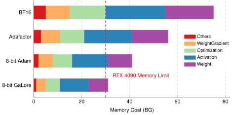](https://mlsysbook.ai/contents/core/training/033a8078b470c1eafa5c3b0c8c2396db97016ced.svg "Figure 6: Memory Footprint Breakdown: Large language models require substantial memory, with optimizer states and gradients often exceeding the size of model weights themselves. This figure quantifies the memory usage of the llama-7B model, revealing how techniques like compression can significantly reduce the overall footprint by minimizing the storage requirements for optimizer data.")
Figure 6: **Memory Footprint Breakdown**: Large language models require substantial memory, with optimizer states and gradients often exceeding the size of model weights themselves. This figure quantifies the memory usage of the llama-7B model, revealing how techniques like compression can significantly reduce the overall footprint by minimizing the storage requirements for optimizer data.
#### Computational Load
The computational cost of parameter updates also depends on the optimizer’s complexity. For gradient descent, each update involves simple gradient calculation and application. More sophisticated optimizers like Adam require additional calculations, such as computing running averages of gradients and their squares. This increases the computational load per parameter update.
The efficiency of these computations on modern hardware like GPUs and TPUs depends on how well the optimizer’s operations can be parallelized. While matrix operations in Adam may be efficiently handled by these accelerators, some operations in complex optimizers might not parallelize well, potentially leading to hardware underutilization.
the choice of optimizer directly impacts both system memory requirements and computational load. More sophisticated optimizers often trade increased memory usage and computational complexity for potentially faster convergence, presenting important considerations for system design and resource allocation in ML systems.
#### Batch Size and Parameter Updates
Batch size, a critical hyperparameter in machine learning systems, significantly influences the parameter update process, memory usage, and hardware efficiency. It determines the number of training examples processed in a single iteration before the model parameters are updated.
Larger batch sizes generally provide more accurate gradient estimates, potentially leading to faster convergence and more stable parameter updates. However, they also increase memory demands proportionally: \\\[ \\text{Memory for Batch} = \\text{Batch Size} \\times \\text{Size of One Training Example} \\\]
This increase in memory usage directly affects the parameter update process, as it determines how much data is available for computing gradients in each iteration.
Building on the efficiency patterns established in previous sections, larger batches improve hardware utilization, particularly on GPUs and TPUs optimized for parallel processing. This leads to more efficient parameter updates and faster training times, provided sufficient memory is available.
As discussed earlier, this computational efficiency comes with memory costs. Systems with limited memory must reduce batch size, creating the same fundamental trade-offs that shape training system architecture throughout.
The choice of batch size interacts with various aspects of the optimization process. For instance, it affects the frequency of parameter updates: larger batches result in less frequent but potentially more impactful updates. Batch size influences the behavior of adaptive optimization algorithms, which may need to be tuned differently depending on the batch size. In distributed training scenarios, batch size often determines the degree of data parallelism, impacting how gradient computations and parameter updates are distributed across devices.
Determining the optimal batch size involves balancing these factors within hardware constraints. It often requires experimentation to find the sweet spot that maximizes both learning efficiency and hardware utilization while ensuring effective parameter updates.
**Self-Check: Question 1.4**
1. Which component of the pipeline architecture is primarily responsible for transforming raw data into a format suitable for model training?
1. Data Pipeline
2. Training Loop
3. Evaluation Pipeline
4. Optimizer
2. Explain how the integration of the data pipeline, training loop, and evaluation pipeline contributes to the efficiency of an ML training system.
3. True or False: The evaluation pipeline operates independently of the training loop and does not impact the training process.
4. The throughput of preprocessing operations can be expressed mathematically as: \_\_\_\_.
5. Order the following stages in the data pipeline: (1) Batching, (2) Format Conversion, (3) Processing.
[See Answers →](https://mlsysbook.ai/contents/core/training/training.html#quiz-answer-sec-ai-training-pipeline-architecture-622a)
Pipeline Optimizations
----------------------
Even well-designed pipeline architectures rarely achieve optimal performance without targeted optimization. The gap between theoretical hardware capability and realized training throughput often reaches 50-70%: GPUs advertised at 300 TFLOPS may deliver only 90-150 TFLOPS for training workloads, and distributed systems with aggregate 1000 TFLOPS capacity frequently achieve under 500 TFLOPS effective throughput ([L. Wang et al. 2018](https://mlsysbook.ai/contents/core/training/training.html#ref-wang2019superneurons)
). This efficiency gap stems from systematic bottlenecks that optimization techniques can address.
Wang, Linnan, Jinmian Ye, Yiyang Zhao, Wei Wu, Ang Li, Shuaiwen Leon Song, Zenglin Xu, and Tim Kraska. 2018. “Superneurons: Dynamic GPU Memory Management for Training Deep Neural Networks.” In _Proceedings of the 23rd ACM SIGPLAN Symposium on Principles and Practice of Parallel Programming_, 41–53. ACM. [https://doi.org/10.1145/3178487.3178491](https://doi.org/10.1145/3178487.3178491)
.
The following table provides a roadmap for matching optimization techniques to the bottlenecks they solve, serving as a practical guide for systematic performance improvement:
Table 4: **Optimization Technique Roadmap**: Each primary bottleneck category has targeted solutions that address specific performance constraints. This mapping guides systematic optimization by matching techniques to profiling results.
| | |
| --- | --- |
| **Data Movement Latency** | Prefetching & Pipeline Overlapping |
| **Compute Throughput** | Mixed-Precision Training |
| **Memory Capacity** | Gradient Accumulation & Activation Checkpointing |
Training pipeline performance is constrained by three primary bottlenecks that determine overall system efficiency ([Table 4](https://mlsysbook.ai/contents/core/training/training.html#tbl-optimization-roadmap)
): data movement latency, computational throughput limitations, and memory capacity constraints. Data movement latency emerges when training batches cannot flow from storage through preprocessing to compute units fast enough to keep accelerators utilized. Computational throughput limitations occur when mathematical operations execute below hardware peak performance due to suboptimal parallelization, precision choices, or kernel inefficiencies. Memory capacity constraints restrict both the model sizes we can train and the batch sizes we can process, directly limiting both model complexity and training efficiency. These bottlenecks manifest differently across system scales—a 100GB model faces different constraints than a 1GB model—but their systematic identification and mitigation follows consistent principles.
These bottlenecks interact in complex ways. When data loading becomes a bottleneck, GPUs sit idle waiting for batches. When computation is suboptimal, memory bandwidth goes underutilized. When memory is constrained, we resort to smaller batches that reduce GPU efficiency. The optimization challenge involves identifying which bottleneck currently limits performance, then selecting techniques that address that specific constraint without introducing new bottlenecks elsewhere.
### Systematic Optimization Framework
The pipeline architecture established above creates opportunities for targeted optimizations. Effective optimization follows a systematic methodology that applies regardless of system scale or model architecture. This three-phase framework provides the foundation for all optimization work: profile to identify bottlenecks, select appropriate techniques for the identified constraints, and compose solutions that address multiple bottlenecks simultaneously without creating conflicts.
The profiling phase employs tools like PyTorch Profiler, TensorFlow Profiler, or NVIDIA Nsight Systems to reveal where time is spent during training iterations. These are the same profiling approaches introduced in the overview—now applied systematically to quantify which bottleneck dominates. A profile might show 40% of time in data loading, 35% in computation, and 25% in memory operations—clearly indicating data loading as the primary target for optimization.
The selection phase matches optimization techniques to identified bottlenecks. Each technique we examine targets specific constraints: prefetching addresses data movement latency, mixed-precision training tackles both computational throughput and memory constraints, and gradient accumulation manages memory limitations. Selection requires understanding not just which bottleneck exists, but the characteristics of the hardware, model architecture, and training configuration that influence technique effectiveness.
The composition phase combines multiple techniques to achieve cumulative benefits. Prefetching and mixed-precision training complement each other—one addresses data loading, the other computation and memory—allowing simultaneous application. However, some combinations create conflicts: aggressive prefetching increases memory pressure, potentially conflicting with memory-constrained configurations. Successful composition requires understanding technique interactions and dependencies.
This systematic framework—profile, select, compose—applies three core optimization techniques to the primary bottleneck categories. Prefetching and overlapping targets data movement latency by coordinating data transfer with computation. Mixed-precision training addresses both computational throughput and memory constraints through reduced precision arithmetic. Gradient accumulation and checkpointing manages memory constraints by trading computation for memory usage. These techniques are not mutually exclusive; effective optimization often combines multiple approaches to achieve cumulative benefits.
### Production Optimization Decision Framework
While the systematic framework establishes methodology, production environments introduce additional operational constraints. The production decision framework extends the systematic approach with operational factors that influence technique selection in real deployment contexts.
Production optimization decisions must balance performance improvements against implementation complexity, operational monitoring requirements, and system reliability. Four factors guide technique selection: performance impact potential quantifies expected speedup or memory savings, implementation complexity assesses development and debugging effort required, operational overhead evaluates ongoing monitoring and maintenance needs, and system reliability implications examines how techniques affect fault tolerance and reproducibility.
High-impact, low-complexity optimizations like data prefetching should be implemented first, providing immediate benefits with minimal risk. Complex optimizations such as gradient checkpointing require careful cost-benefit analysis including development time, debugging complexity, and ongoing maintenance requirements. We examine each optimization technique through this production lens, providing specific guidance on implementation priorities, monitoring requirements, and operational considerations that enable practitioners to make informed decisions for their specific deployment environments.
### Data Prefetching and Pipeline Overlapping
To illustrate the systematic framework in action, we begin with prefetching and overlapping techniques that target data movement latency bottlenecks by coordinating data transfer with computation. This optimization proves most effective when profiling reveals that computational units remain idle while waiting for data transfers to complete.
Training machine learning models involves significant data movement between storage, memory, and computational units. The data pipeline consists of sequential transfers: from disk storage to CPU memory, CPU memory to GPU memory, and through the GPU processing units. In standard implementations, each transfer must complete before the next begins, as shown in [Figure 7](https://mlsysbook.ai/contents/core/training/training.html#fig-fetching-naive)
, resulting in computational inefficiencies.
[](https://mlsysbook.ai/contents/core/training/2fb59ac417cf992e9d61cf8625d17b2dd1779086.svg "Figure 7: Sequential Data Transfer: Standard data fetching pipelines execute transfers from disk to CPU, CPU to GPU, and through GPU processing one at a time, creating bottlenecks and limiting computational throughput during model training. This serial approach prevents overlapping computation and data movement, hindering efficient resource utilization.")
Figure 7: **Sequential Data Transfer**: Standard data fetching pipelines execute transfers from disk to CPU, CPU to GPU, and through GPU processing one at a time, creating bottlenecks and limiting computational throughput during model training. This serial approach prevents overlapping computation and data movement, hindering efficient resource utilization.
Prefetching addresses these inefficiencies by loading data into memory before its scheduled computation time. During the processing of the current batch, the system loads and prepares subsequent batches, maintaining a consistent supply of ready data ([Abadi et al. 2015](https://mlsysbook.ai/contents/core/training/training.html#ref-tensorflow_data_2015)
).
Abadi, Martín, Ashish Agarwal, Paul Barham, et al. 2015. “TensorFlow: Large-Scale Machine Learning on Heterogeneous Systems.” Google Brain.
Overlapping builds upon prefetching by coordinating multiple pipeline stages to execute concurrently. The system processes the current batch while simultaneously preparing future batches through data loading and preprocessing operations. This coordination establishes a continuous data flow through the training pipeline, as illustrated in [Figure 8](https://mlsysbook.ai/contents/core/training/training.html#fig-fetching-optimized)
.
[](https://mlsysbook.ai/contents/core/training/e12fcc2d3c87925de0cc91f4d3b8536053e523f7.svg "Figure 8: Pipeline Parallelism: Overlapping computation and data fetching reduces overall job completion time by concurrently processing data and preparing subsequent batches. This optimization achieves a 40% speedup, finishing in 00:40 seconds compared to 01:30 seconds with naive sequential fetching.")
Figure 8: **Pipeline Parallelism**: Overlapping computation and data fetching reduces overall job completion time by concurrently processing data and preparing subsequent batches. This optimization achieves a 40% speedup, finishing in 00:40 seconds compared to 01:30 seconds with naive sequential fetching.
These optimization techniques demonstrate particular value in scenarios involving large-scale datasets, preprocessing-intensive data, multi-GPU training configurations, or high-latency storage systems. The following section examines the specific mechanics of implementing these techniques in modern training systems.
#### Prefetching Mechanics
Prefetching and overlapping optimize the training pipeline by enabling different stages of data processing and computation to operate concurrently rather than sequentially. These techniques maximize resource utilization by addressing bottlenecks in data transfer and preprocessing.
As you recall, training data undergoes three main stages: retrieval from storage, transformation into a suitable format, and utilization in model training. An unoptimized pipeline executes these stages sequentially. The GPU remains idle during data fetching and preprocessing, waiting for data preparation to complete. This sequential execution creates significant inefficiencies in the training process.
Prefetching eliminates waiting time by loading data asynchronously during model computation. Data loaders operate as separate threads or processes, preparing the next batch while the current batch trains. This ensures immediate data availability for the GPU when the current batch completes.
Overlapping extends this efficiency by coordinating all three pipeline stages simultaneously. As the GPU processes one batch, preprocessing begins on the next batch, while data fetching starts for the subsequent batch. This coordination maintains constant activity across all pipeline stages.
Modern machine learning frameworks implement these techniques through built-in utilities. PyTorch’s `DataLoader` class demonstrates this implementation. An example of this usage is shown in [Listing 2](https://mlsysbook.ai/contents/core/training/training.html#lst-dataloader_usage)
.
Listing 2: **Pipeline Optimization**: Machine learning workflows benefit from efficient data handling through batching and prefetching to maintain constant GPU utilization.
loader = DataLoader(
dataset, batch_size=32, num_workers=4, prefetch_factor=2
)
The parameters `num_workers` and `prefetch_factor` control parallel processing and data buffering. Multiple worker processes handle data loading and preprocessing concurrently, while prefetch\_factor determines the number of batches prepared in advance.
Buffer management plays a key role in pipeline efficiency. The prefetch buffer size requires careful tuning to balance resource utilization. A buffer that is too small causes the GPU to wait for data preparation, reintroducing the idle time these techniques aim to eliminate. Conversely, allocating an overly large buffer consumes memory that could otherwise store model parameters or larger batch sizes.
The implementation relies on effective CPU-GPU coordination. The CPU manages data preparation tasks while the GPU handles computation. This division of labor, combined with storage I/O operations, creates an efficient pipeline that minimizes idle time across hardware resources.
These optimization techniques yield particular benefits in scenarios involving slow storage access, complex data preprocessing, or large datasets. These techniques offer specific advantages in different training contexts depending on the computational and data characteristics.
#### Prefetching Benefits
Prefetching and overlapping are techniques that significantly enhance the efficiency of training pipelines by addressing key bottlenecks in data handling and computation. To illustrate the impact of these benefits, [Table 5](https://mlsysbook.ai/contents/core/training/training.html#tbl-prefetching)
presents the following comparison:
Table 5: **Pipeline Optimization**: Prefetching and overlapping maximize hardware utilization and reduce training time by enabling parallel data loading and computation, overcoming bottlenecks inherent in sequential pipelines. Increased resource usage and adaptability to varying bottlenecks demonstrate the scalability advantages of these techniques.
| | | |
| --- | --- | --- |
| **GPU Utilization** | Frequent idle periods | Near-constant utilization |
| **Training Time** | Longer due to sequential operations | Reduced through parallelism |
| **Resource Usage** | Often suboptimal | Maximized across available hardware |
| **Scalability** | Limited by slowest component | Adaptable to various bottlenecks |
One of the most critical advantages of these methods is the improvement in GPU utilization. In traditional, unoptimized pipelines, the GPU often remains idle while waiting for data to be fetched and preprocessed. This idle time creates inefficiencies, especially in workflows where data augmentation or preprocessing involves complex transformations. By introducing asynchronous data loading and overlapping, these techniques ensure that the GPU consistently has data ready to process, eliminating unnecessary delays.
Another important benefit is the reduction in overall training time. Prefetching and overlapping allow the computational pipeline to operate continuously, with multiple stages working simultaneously rather than sequentially. For example, while the GPU processes the current batch, the data loader fetches and preprocesses the next batch, ensuring a steady flow of data through the system. This parallelism minimizes latency between training iterations, allowing for faster completion of training cycles, particularly in scenarios involving large-scale datasets.
These techniques are highly scalable and adaptable to various hardware configurations. Prefetching buffers and overlapping mechanisms can be tuned to match the specific requirements of a system, whether the bottleneck lies in slow storage, limited network bandwidth, or computational constraints. By aligning the data pipeline with the capabilities of the underlying hardware, prefetching and overlapping maximize resource utilization, making them invaluable for large-scale machine learning workflows.
Overall, prefetching and overlapping directly address some of the most common inefficiencies in training pipelines. By optimizing data flow and computation, these methods not only improve hardware efficiency but also enable the training of more complex models within shorter timeframes.
#### Data Pipeline Optimization Applications
Prefetching and overlapping are highly versatile techniques that can be applied across various machine learning domains and tasks to enhance pipeline efficiency. Their benefits are most evident in scenarios where data handling and preprocessing are computationally expensive or where large-scale datasets create potential bottlenecks in data transfer and loading.
One of the primary use cases is in computer vision, where datasets often consist of high-resolution images requiring extensive preprocessing. Tasks such as image classification, object detection, or semantic segmentation typically involve operations like resizing, normalization, and data augmentation, all of which can significantly increase preprocessing time. By employing prefetching and overlapping, these operations can be carried out concurrently with computation, ensuring that the GPU remains busy during the training process.
For example, a typical image classification pipeline might include random cropping (10 ms), color jittering (15 ms), and normalization (5 ms). Without prefetching, these 30 ms of preprocessing would delay each training step. Prefetching allows these operations to occur during the previous batch’s computation.
NLP workflows also benefit from these techniques, particularly when working with large corpora of text data. For instance, preprocessing text data involves tokenization (converting words to numbers), padding sequences to equal length, and potentially subword tokenization. In a BERT model training pipeline, these steps might process thousands of sentences per batch. Prefetching allows this text processing to happen concurrently with model training. Prefetching ensures that these transformations occur in parallel with training, while overlapping optimizes data transfer and computation. This is especially useful in transformer-based models like BERT or GPT, which require consistent throughput to maintain efficiency given their high computational demand.
Distributed training systems involve multiple GPUs or nodes, present another critical application for prefetching and overlapping. In distributed setups, network latency and data transfer rates often become the primary bottleneck. Prefetching mitigates these issues by ensuring that data is ready and available before it is required by any specific GPU. Overlapping further optimizes distributed training pipelines by coordinating the data preprocessing on individual nodes while the central computation continues, thus reducing overall synchronization delays.
Beyond these domains, prefetching and overlapping are particularly valuable in workflows involving large-scale datasets stored on remote or cloud-based systems. When training on cloud platforms, the data may need to be fetched over a network or from distributed storage, which introduces additional latency. Using prefetching and overlapping in such cases helps minimize the impact of these delays, ensuring that training proceeds smoothly despite slower data access speeds.
These use cases illustrate how prefetching and overlapping address inefficiencies in various machine learning pipelines. By optimizing the flow of data and computation, these techniques enable faster, more reliable training workflows across a wide range of applications.
#### Pipeline Optimization Implementation Challenges
While prefetching and overlapping are useful techniques for optimizing training pipelines, their implementation comes with certain challenges and trade-offs. Understanding these limitations is important for effectively applying these methods in real-world machine learning workflows.
One of the primary challenges is the increased memory usage that accompanies prefetching and overlapping. By design, these techniques rely on maintaining a buffer of prefetched data batches, which requires additional memory resources. For large datasets or high-resolution inputs, this memory demand can become significant, especially when training on GPUs with limited memory capacity. If the buffer size is not carefully tuned, it may lead to out-of-memory errors, forcing practitioners to reduce batch sizes or adjust other parameters, which can impact overall efficiency.
For example, with a prefetch factor of 2 and batch size of 256 high-resolution images (\\(1024\\times1024\\) pixels), the buffer might require an additional 2 GB of GPU memory. This becomes particularly challenging when training vision models that already require significant memory for their parameters and activations.
Another difficulty lies in tuning the parameters that control prefetching and overlapping. Settings such as `num_workers` and `prefetch_factor` in PyTorch, or buffer sizes in other frameworks, need to be optimized for the specific hardware and workload. For instance, increasing the number of worker threads can improve throughput up to a point, but beyond that, it may lead to contention for CPU resources or even degrade performance due to excessive context switching. Determining the optimal configuration often requires empirical testing, which can be time-consuming. A common starting point is to set `num_workers` to the number of CPU cores available. However, on a 16-core system processing large images, using all cores for data loading might leave insufficient CPU resources for other essential operations, potentially slowing down the entire pipeline.
Debugging also becomes more complex in pipelines that employ prefetching and overlapping. Asynchronous data loading and multithreading or multiprocessing introduce potential race conditions, deadlocks, or synchronization issues. Diagnosing errors in such systems can be challenging because the execution flow is no longer straightforward. Developers may need to invest additional effort into monitoring, logging, and debugging tools to ensure that the pipeline operates reliably.
There are scenarios where prefetching and overlapping may offer minimal benefits. For instance, in systems where storage access or network bandwidth is significantly faster than the computation itself, these techniques might not noticeably improve throughput. In such cases, the additional complexity and memory overhead introduced by prefetching may not justify its use.
Finally, prefetching and overlapping require careful coordination across different components of the training pipeline, such as storage, CPUs, and GPUs. Poorly designed pipelines can lead to imbalances where one stage becomes a bottleneck, negating the advantages of these techniques. For example, if the data loading process is too slow to keep up with the GPU’s processing speed, the benefits of overlapping will be limited.
Despite these challenges, prefetching and overlapping remain essential tools for optimizing training pipelines when used appropriately. By understanding and addressing their trade-offs, practitioners can implement these techniques effectively, ensuring smoother and more efficient machine learning workflows.
### Mixed-Precision Training
While prefetching optimizes data movement, mixed-precision training addresses both computational throughput limitations and memory capacity constraints by strategically using reduced precision arithmetic where possible while maintaining numerical stability. This technique proves most effective when profiling reveals that training is constrained by GPU memory capacity or when computational units are not fully utilized due to memory bandwidth limitations.
Mixed-precision training combines different numerical precisions during model training to optimize computational efficiency. This approach uses combinations of FP32, 16-bit floating-point (FP16), and brain floating-point (bfloat16) formats to reduce memory usage and speed up computation while preserving model accuracy ([Micikevicius et al. 2017](https://mlsysbook.ai/contents/core/training/training.html#ref-micikevicius2017mixed)
; [Y. Wang and Kanwar 2019](https://mlsysbook.ai/contents/core/training/training.html#ref-wang_bfloat16_2019)
).
Wang, Y., and P. Kanwar. 2019. “BFloat16: The Secret to High Performance on Cloud TPUs.” _Google Cloud Blog_.
A neural network trained in FP32 requires 4 bytes per parameter, while both FP16 and bfloat16 use 2 bytes. For a model with \\(10^9\\) parameters, this reduction cuts memory usage from 4 GB to 2 GB. This memory reduction enables larger batch sizes and deeper architectures on the same hardware.
The numerical precision differences between these formats shape their use cases. FP32 represents numbers from approximately \\(\\pm1.18 \\times 10^{-38}\\) to \\(\\pm3.4 \\times 10^{38}\\) with 7 decimal digits of precision. FP16 ranges from \\(\\pm6.10 \\times 10^{-5}\\) to \\(\\pm65,504\\) with 3-4 decimal digits of precision. Bfloat16, developed by Google Brain, maintains the same dynamic range as FP32 (\\(\\pm1.18 \\times 10^{-38}\\) to \\(\\pm3.4 \\times 10^{38}\\)) but with reduced precision (3-4 decimal digits). This range preservation makes bfloat16 particularly suited for deep learning training, as it handles large and small gradients more effectively than FP16.
The hybrid approach proceeds in three main phases, as illustrated in [Figure 9](https://mlsysbook.ai/contents/core/training/training.html#fig-mixed-precision)
. During the forward pass, input data converts to reduced precision (FP16 or bfloat16), and matrix multiplications execute in this format, including activation function computations. In the gradient computation phase, the backward pass calculates gradients in reduced precision, but results are stored in FP32 master weights. Finally, during weight updates, the optimizer updates the main weights in FP32, and these updated weights convert back to reduced precision for the next forward pass.
[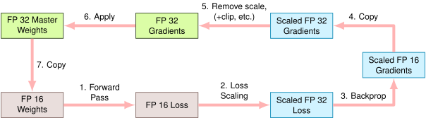](https://mlsysbook.ai/contents/core/training/26cb3e67d0a38aec9cc98301abf8863c9e8e89ea.svg "Figure 9: Mixed Precision Training: Reduced precision formats (FP16, bfloat16) accelerate deep learning by decreasing memory bandwidth and computational requirements during both forward and backward passes. Master weights stored in FP32 precision accumulate updates from reduced precision gradients, preserving accuracy while leveraging performance gains from lower precision arithmetic.")
Figure 9: **Mixed Precision Training**: Reduced precision formats (FP16, bfloat16) accelerate deep learning by decreasing memory bandwidth and computational requirements during both forward and backward passes. Master weights stored in FP32 precision accumulate updates from reduced precision gradients, preserving accuracy while leveraging performance gains from lower precision arithmetic.
Modern hardware architectures are specifically designed to accelerate reduced precision computations. GPUs from NVIDIA include Tensor Cores optimized for FP16 and bfloat16 operations ([Jia et al. 2018](https://mlsysbook.ai/contents/core/training/training.html#ref-nvidia_tensors_fp16_2017)
). Google’s TPUs natively support bfloat16, as this format was specifically designed for machine learning workloads. These architectural optimizations typically enable an order of magnitude higher computational throughput for reduced precision operations compared to FP32, making mixed-precision training particularly efficient on modern hardware.
Jia, Xianyan, Shutao Song, Wei He, Yangzihao Wang, Haidong Rong, Feihu Zhou, Liqiang Xie, et al. 2018. “Highly Scalable Deep Learning Training System with Mixed-Precision: Training ImageNet in Four Minutes.” _arXiv Preprint arXiv:1807.11205_, July. [http://arxiv.org/abs/1807.11205v1](http://arxiv.org/abs/1807.11205v1)
.
#### FP16 Computation
The majority of operations in mixed-precision training, such as matrix multiplications and activation functions, are performed in FP16. The reduced precision allows these calculations to be executed faster and with less memory consumption compared to FP32. FP16 operations are particularly effective on modern GPUs equipped with Tensor Cores, which are designed to accelerate computations involving half-precision values. These cores perform FP16 operations natively, resulting in significant speedups.
#### FP32 Accumulation
While FP16 is efficient, its limited precision can lead to numerical instability, especially in critical operations like gradient updates. To mitigate this, mixed-precision training retains FP32 precision for certain steps, such as weight updates and gradient accumulation. By maintaining higher precision for these calculations, the system avoids the risk of gradient underflow or overflow, ensuring the model converges correctly during training.
#### Loss Scaling
One of the key challenges with FP16 is its reduced dynamic range[27](https://mlsysbook.ai/contents/core/training/training.html#fn27)
, which increases the likelihood of gradient values becoming too small to be represented accurately. Loss scaling addresses this issue by temporarily amplifying gradient values during backpropagation. Specifically, the loss value is scaled by a large factor (e.g., \\(2^{10}\\)) before gradients are computed, ensuring they remain within the representable range of FP16.
27 **FP16 Dynamic Range**: IEEE 754 half-precision (FP16) has only 5 exponent bits vs. 8 in FP32, limiting its range to ±65,504 (vs. ±3.4×10³⁸ for FP32). More critically, FP16’s smallest representable positive number is 6×10⁻⁸, while gradients in deep networks often fall below 10⁻¹⁰. This mismatch causes gradient underflow, where tiny but important gradients become zero, stalling training, hence the need for loss scaling techniques. Once the gradients are computed, the scaling factor is reversed during the weight update step to restore the original gradient magnitude. This process allows FP16 to be used effectively without sacrificing numerical stability.
Modern machine learning frameworks, such as PyTorch and TensorFlow, provide built-in support for mixed-precision training. These frameworks abstract the complexities of managing different precisions, enabling practitioners to implement mixed-precision workflows with minimal effort. For instance, PyTorch’s `torch.cuda.amp` (Automatic Mixed Precision) library automates the process of selecting which operations to perform in FP16 or FP32, as well as applying loss scaling when necessary.
Combining FP16 computation, FP32 accumulation, and loss scaling allows us to achieve mixed-precision training, resulting in a significant reduction in memory usage and computational overhead without compromising the accuracy or stability of the training process. The following sections will explore the practical advantages of this approach and its impact on modern machine learning workflows.
#### Mixed-Precision Benefits
Mixed-precision training offers advantages that make it an optimization technique for modern machine learning workflows. By reducing memory usage and computational load, it enables practitioners to train larger models, process bigger batches, and achieve faster results, all while maintaining model accuracy and convergence.
Mixed-precision training reduces memory consumption. FP16 computations require only half the memory of FP32 computations, which directly reduces the storage required for activations, weights, and gradients during training. For instance, a transformer model with 1 billion parameters requires 4 GB of memory for weights in FP32, but only 2 GB in FP16. This memory efficiency allows for larger batch sizes, which can lead to more stable gradient estimates and faster convergence. With less memory consumed per operation, practitioners can train deeper and more complex models on the same hardware, unlocking capabilities that were previously limited by memory constraints.
Mixed-precision training also accelerates computations. Modern GPUs, such as those equipped with Tensor Cores, are specifically optimized for FP16 operations. These cores enable hardware to process more operations per cycle compared to FP32, resulting in faster training times. Leveraging the matrix multiplication patterns detailed earlier, FP16 can achieve 2-3\\(\\times\\) speedup compared to FP32 for these dominant operations. This computational speedup becomes noticeable in large-scale models, such as transformers and convolutional neural networks, where these patterns concentrate the computational workload.
Mixed-precision training also improves hardware utilization by better matching the capabilities of modern accelerators. In traditional FP32 workflows, the computational throughput of GPUs is often underutilized due to their design for parallel processing. FP16 operations, being less demanding, allow more computations to be performed simultaneously, ensuring that the hardware operates closer to its full capacity.
Finally, mixed-precision training aligns well with the requirements of distributed and cloud-based systems. In distributed training, where large-scale models are trained across multiple GPUs or nodes, memory and bandwidth become critical constraints. By reducing the size of tensors exchanged between devices, mixed precision not only speeds up inter-device communication but also decreases overall resource demands. This makes it particularly effective in environments where scalability and cost-efficiency are priorities.
Overall, the benefits of mixed-precision training extend beyond performance improvements. By optimizing memory usage and computation, this technique enables machine learning practitioners to train advanced models more efficiently, making it a cornerstone of modern machine learning.
GPT-2 Mixed Precision Training Impact
GPT-2 training heavily relies on mixed-precision (FP16) to fit within GPU memory constraints.
**Memory Savings**
FP32 Baseline:
* Parameters: 1.5B × 4 bytes = 6.0 GB
* Activations (batch=32): ~65 GB
* Gradients: 6.0 GB
* Total: ~77 GB (exceeds any single GPU)
FP16 Mixed Precision:
* Parameters (FP16): 1.5B × 2 bytes = 3.0 GB
* Activations (FP16): ~32.6 GB
* Gradients (FP16): 3.0 GB
* Optimizer state (FP32 master weights): 12.0 GB (Adam m, v)
* Total: ~51 GB (still tight, but manageable with optimizations)
With Mixed Precision + Gradient Checkpointing:
* Activations reduced to ~8 GB (recompute during backward)
* Total: ~26 GB → fits comfortably in 32GB V100
**Computational Speedup**
On NVIDIA V100 (Tensor Cores enabled):
* FP32 throughput: ~90 samples/sec
* FP16 throughput: ~220 samples/sec
* Speedup: 2.4× faster training
**Critical Implementation Details**
1. Loss Scaling: Start with scale=2^15, dynamically reduce if overflow detected. Gradients in attention layers can range from 10^-6 to 10^3, so loss scaling prevents underflow.
2. FP32 Master Weights: Optimizer updates in FP32 prevent weight stagnation. Small learning rate (2.5e-4) × FP16 gradient might round to zero; FP32 accumulation preserves these tiny updates.
3. Selective FP32 Operations:
* LayerNorm: Computed in FP32 (requires high precision for variance calculation)
* Softmax: Computed in FP32 (exponentials need full range)
* All else: FP16
**Training Cost Impact**
* FP32: ~$50,000 for 2 weeks on 32 V100s
* FP16: ~$28,000 for 1.2 weeks on 32 V100s
* Savings: $22,000 + 6 days faster iteration
**Quality Impact:** Minimal. GPT-2 perplexity within 0.5% of FP32 baseline, well within noise margin.
#### Mixed-Precision Training Applications
Mixed-precision training has become essential in machine learning workflows, particularly in domains and scenarios where computational efficiency and memory optimization are critical. Its ability to enable faster training and larger model capacities makes it highly applicable across a variety of machine learning tasks and architectures.
One of the most prominent use cases is in training large-scale machine learning models. In natural language processing, models such as BERT (345M parameters), GPT-3 (175B parameters), and Transformer-based architectures exemplify the computational patterns discussed throughout this chapter. Mixed-precision training allows these models to operate with larger batch sizes or deeper configurations, facilitating faster convergence and improved accuracy on massive datasets.
In computer vision, tasks such as image classification, object detection, and segmentation often require handling high-resolution images and applying computationally intensive convolutional operations. By leveraging mixed-precision training, these workloads can be executed more efficiently, enabling the training of advanced architectures like ResNet, EfficientNet, and vision transformers within practical resource limits.
Mixed-precision training is also particularly valuable in reinforcement learning (RL), where models interact with environments to optimize decision-making policies. RL often involves high-dimensional state spaces and requires substantial computational resources for both model training and simulation. Mixed precision reduces the overhead of these processes, allowing researchers to focus on larger environments and more complex policy networks.
Another critical application is in distributed training systems. When training models across multiple GPUs or nodes, memory and bandwidth become limiting factors for scalability. Mixed precision addresses these issues by reducing the size of activations, weights, and gradients exchanged between devices. For example, in a distributed training setup with 8 GPUs, reducing tensor sizes from FP32 to FP16 can halve the communication bandwidth requirements from 320 GB/s to 160 GB/s. This optimization is beneficial in cloud-based environments, where resource allocation and cost efficiency are critical.
Mixed-precision training is increasingly used in areas such as speech processing, generative modeling, and scientific simulations. Models in these fields often have large data and parameter requirements that can push the limits of traditional FP32 workflows. By optimizing memory usage and leveraging the speedups provided by Tensor Cores, practitioners can train advanced models faster and more cost-effectively.
The adaptability of mixed-precision training to diverse tasks and domains underscores its importance in modern machine learning. Whether applied to large-scale natural language models, computationally intensive vision architectures, or distributed training environments, this technique empowers researchers and engineers to push the boundaries of what is computationally feasible.
#### Mixed-Precision Training Limitations
While mixed-precision training offers significant advantages in terms of memory efficiency and computational speed, it also introduces several challenges and trade-offs that must be carefully managed to ensure successful implementation.
One of the primary challenges lies in the reduced precision of FP16. While FP16 computations are faster and require less memory, their limited dynamic range \\((\\pm65,504)\\) can lead to numerical instability, particularly during gradient computations. Small gradient values below \\(6 \\times 10^{-5}\\) become too small to be represented accurately in FP16, resulting in underflow. While loss scaling addresses this by multiplying gradients by factors like \\(2^{8}\\) to \\(2^{14}\\), implementing and tuning this scaling factor adds complexity to the training process.
Another trade-off involves the increased risk of convergence issues. While many modern machine learning tasks perform well with mixed-precision training, certain models or datasets may require higher precision to achieve stable and reliable results. For example, recurrent neural networks with long sequences often accumulate numerical errors in FP16, requiring careful gradient clipping and precision management. In such cases, practitioners may need to experiment with selectively enabling or disabling FP16 computations for specific operations, which can complicate the training workflow.
Debugging and monitoring mixed-precision training also require additional attention. Numerical issues such as NaN (Not a Number) values in gradients or activations are more common in FP16 workflows and may be difficult to trace without proper tools and logging. For instance, gradient explosions in deep networks might manifest differently in mixed precision, appearing as infinities in FP16 before they would in FP32. Frameworks like PyTorch and TensorFlow provide utilities for debugging mixed-precision training, but these tools may not catch every edge case, especially in custom implementations.
Another challenge is the dependency on specialized hardware. Mixed-precision training relies heavily on GPU architectures optimized for FP16 operations, such as Tensor Cores in NVIDIA’s GPUs. While these GPUs are becoming increasingly common, not all hardware supports mixed-precision operations, limiting the applicability of this technique in some environments.
Finally, there are scenarios where mixed-precision training may not provide significant benefits. Models with relatively low computational demand (less than 10M parameters) or small parameter sizes may not fully utilize the speedups offered by FP16 operations. In such cases, the additional complexity of mixed-precision workflows may outweigh their potential advantages.
Despite these challenges, mixed-precision training remains a highly effective optimization technique for most large-scale machine learning tasks. By understanding and addressing its trade-offs, practitioners can use its benefits while minimizing potential drawbacks, ensuring efficient and reliable training workflows.
### Gradient Accumulation and Checkpointing
Complementing mixed-precision’s approach to memory optimization, gradient accumulation and checkpointing techniques address memory capacity constraints by trading computational time for reduced memory usage. These techniques prove most effective when profiling reveals that training is limited by available memory rather than computational throughput, enabling larger models or batch sizes on memory-constrained hardware.
Training large machine learning models often requires significant memory resources, particularly for storing three key components: activations (intermediate layer outputs), gradients (parameter updates), and model parameters (weights and biases) during forward and backward passes. However, memory constraints on GPUs can limit the batch size or the complexity of models that can be trained on a given device.
Gradient accumulation and activation checkpointing are two techniques designed to address these limitations by optimizing how memory is utilized during training. Both techniques enable researchers and practitioners to train larger and more complex models, making them indispensable tools for modern deep learning workflows. Understanding when to apply these techniques requires careful analysis of memory usage patterns and performance bottlenecks in specific training scenarios.
#### Gradient Accumulation and Checkpointing Mechanics
Gradient accumulation and activation checkpointing operate on distinct principles, but both aim to optimize memory usage during training by modifying how forward and backward computations are handled.
##### Gradient Accumulation
Gradient accumulation simulates larger batch sizes by splitting a single effective batch into smaller “micro-batches.” As illustrated in [Figure 10](https://mlsysbook.ai/contents/core/training/training.html#fig-grad-accumulation)
, during each forward and backward pass, the gradients for a micro-batch are computed and added to an accumulated gradient buffer. Instead of immediately applying the gradients to update the model parameters, this process repeats for several micro-batches. Once the gradients from all micro-batches in the effective batch are accumulated, the parameters are updated using the combined gradients.
[](https://mlsysbook.ai/contents/core/training/f6c84d8a5dfe9bec3ca0992c024cbc508ef3bb1c.svg "Figure 10: Gradient Accumulation: Effective batch size increases without increasing per-step memory requirements by accumulating gradients from multiple micro-batches before updating model parameters, simulating training with a larger batch. This technique enables training with large models or datasets when memory is limited, improving training stability and potentially generalization performance.")
Figure 10: **Gradient Accumulation**: Effective batch size increases without increasing per-step memory requirements by accumulating gradients from multiple micro-batches before updating model parameters, simulating training with a larger batch. This technique enables training with large models or datasets when memory is limited, improving training stability and potentially generalization performance.
This process allows models to achieve the benefits of training with larger batch sizes, such as improved gradient estimates and convergence stability, without requiring the memory to store an entire batch at once. For instance, in PyTorch, this can be implemented by adjusting the learning rate proportionally to the number of accumulated micro-batches and calling `optimizer.step()` only after processing the entire effective batch.
The key steps in gradient accumulation are:
1. Perform the forward pass for a micro-batch.
2. Compute the gradients during the backward pass.
3. Accumulate the gradients into a buffer without updating the model parameters.
4. Repeat steps 1-3 for all micro-batches in the effective batch.
5. Update the model parameters using the accumulated gradients after all micro-batches are processed.
##### Activation Checkpointing
Activation checkpointing reduces memory usage during the backward pass by discarding and selectively recomputing activations. In standard training, activations from the forward pass are stored in memory for use in gradient computations during backpropagation. However, these activations can consume significant memory, particularly in deep networks.
With checkpointing, only a subset of the activations is retained during the forward pass. When gradients need to be computed during the backward pass, the discarded activations are recomputed on demand by re-executing parts of the forward pass, as illustrated in [Figure 11](https://mlsysbook.ai/contents/core/training/training.html#fig-activation-checkpointing)
. This approach trades computational efficiency for memory savings, as the recomputation increases training time but allows deeper models to be trained within limited memory constraints. The figure shows how memory is saved by avoiding storage of unnecessarily large intermediate tensors from the forward pass, and simply recomputing them on demand in the backwards pass.
The implementation involves:
1. Splitting the model into segments.
2. Retaining activations only at the boundaries of these segments during the forward pass.
3. Recomputing activations for intermediate layers during the backward pass when needed.
[](https://mlsysbook.ai/contents/core/training/8e56b9e21c7aea39122553ec6ad59f6d805c06b0.svg "Figure 11: Activation Checkpointing: Trading memory usage for recomputation during backpropagation enables training deeper neural networks. By storing only a subset of activations from the forward pass and recomputing others on demand, this technique reduces peak memory requirements at the cost of increased training time.")
Figure 11: **Activation Checkpointing**: Trading memory usage for recomputation during backpropagation enables training deeper neural networks. By storing only a subset of activations from the forward pass and recomputing others on demand, this technique reduces peak memory requirements at the cost of increased training time.
Frameworks like PyTorch provide tools such as `torch.utils.checkpoint` to simplify this process. Checkpointing is particularly effective for very deep architectures, such as transformers or large convolutional networks, where the memory required for storing activations can exceed the GPU’s capacity.
The synergy between gradient accumulation and checkpointing enables training of larger, more complex models. Gradient accumulation manages memory constraints related to batch size, while checkpointing optimizes memory usage for intermediate activations. Together, these techniques expand the range of models that can be trained on available hardware.
#### Memory and Computational Benefits
Gradient accumulation[28](https://mlsysbook.ai/contents/core/training/training.html#fn28)
and activation checkpointing[29](https://mlsysbook.ai/contents/core/training/training.html#fn29)
provide solutions to the memory limitations often encountered in training large-scale machine learning models. By optimizing how memory is used during training, these techniques enable the development and deployment of complex architectures, even on hardware with constrained resources.
28 **Gradient Accumulation Impact**: Enables effective batch sizes of 2048+ on single GPUs with only 32-64 mini-batch size, essential for transformer training. BERT-Large training uses effective batch size of 256 (accumulated over 8 steps) achieving 99.5% of full-batch performance while reducing memory requirements by 8x. The technique trades 10-15% compute overhead for massive memory savings.
29 **Activation Checkpointing Trade-offs**: Reduces memory usage by 50-90% at the cost of 15-30% additional compute time due to recomputation. For training GPT-3 on V100s, checkpointing enables 2.8x larger models (from 1.3B to 3.7B parameters) within 32GB memory constraints, making it essential for memory-bound large model training despite the compute penalty.
One of the primary benefits of gradient accumulation is its ability to simulate larger batch sizes without increasing the memory requirements for storing the full batch. Larger batch sizes are known to improve gradient estimates, leading to more stable convergence and faster training. With gradient accumulation, practitioners can achieve these benefits while working with smaller micro-batches that fit within the GPU’s memory. This flexibility is useful when training models on high-resolution data, such as large images or 3D volumetric data, where even a single batch may exceed available memory.
Activation checkpointing, on the other hand, significantly reduces the memory footprint of intermediate activations during the forward pass. This allows for the training of deeper models, which would otherwise be infeasible due to memory constraints. By discarding and recomputing activations as needed, checkpointing frees up memory that can be used for larger models, additional layers, or higher resolution data. This is especially important in advanced architectures, such as transformers or dense convolutional networks, which require substantial memory to store intermediate computations.
Both techniques enhance the scalability of machine learning workflows. In resource-constrained environments, such as cloud-based platforms or edge devices, these methods provide a means to train models efficiently without requiring expensive hardware upgrades. They enable researchers to experiment with larger and more complex architectures, pushing the boundaries of what is computationally feasible.
Beyond memory optimization, these techniques also contribute to cost efficiency. By reducing the hardware requirements for training, gradient accumulation and checkpointing lower the overall cost of development, making them valuable for organizations working within tight budgets. This is particularly relevant for startups, academic institutions, or projects running on shared computing resources.
Gradient accumulation and activation checkpointing provide both technical and practical advantages. These techniques create a more flexible, scalable, and cost-effective approach to training large-scale models, empowering practitioners to tackle increasingly complex machine learning challenges.
GPT-2 Gradient Accumulation Strategy
GPT-2’s training configuration demonstrates the essential role of gradient accumulation.
**Memory Constraints**
* V100 32GB GPU with gradient checkpointing: Can fit batch\_size=16 (as shown in activation memory example)
* Desired effective batch\_size: 512 (optimal for transformer convergence)
* Problem: 512 ÷ 16 = 32 GPUs needed just for batch size
**Gradient Accumulation Solution**
Instead of 32 GPUs, use 8 GPUs with gradient accumulation:
Configuration:
* Per-GPU micro-batch: 16
* Accumulation steps: 4
* Effective batch per GPU: 16 × 4 = 64
* Global effective batch: 8 GPUs × 64 = **512** ✓
Training Loop:
optimizer.zero_grad()
for step in range(4): # Accumulation steps
micro_batch = next(dataloader) # 16 samples
loss = model(micro_batch) / 4 # Scale loss
loss.backward() # Accumulate gradients
# Now gradients represent 64 samples
all_reduce(gradients) # Sync across 8 GPUs
optimizer.step() # Update with effective batch=512
**Performance Impact**
Without Accumulation (naive approach):
* 32 GPUs × batch\_size=16 = 512 effective batch
* Gradient sync: 32 GPUs → high communication overhead
* Cost: $16/hour × 32 GPUs = $512/hour
With Accumulation (actual GPT-2 approach):
* 8 GPUs × (16 × 4 accumulation) = 512 effective batch
* Gradient sync: Only every 4 steps, only 8 GPUs
* Cost: $16/hour × 8 GPUs = $128/hour
* Savings: $384/hour = 75% cost reduction
**Tradeoff Analysis**
* Compute overhead: 4× forward passes per update = ~8% slower (pipeline overlaps some cost)
* Memory overhead: Gradient accumulation buffer = negligible (gradients already needed)
* Communication benefit: Sync frequency reduced by 4× → communication time drops by 75%
* Cost benefit: Training 2 weeks on 8 GPUs = $21.5K vs. 32 GPUs = $86K
**Convergence Quality**
* Effective batch 512 with accumulation: Perplexity 18.3
* True batch 512 without accumulation: Perplexity 18.2
* Difference: 0.5% (within noise margin)
**Why This Works:** Gradient accumulation is mathematically equivalent to larger batches because gradients are additive: \\\[ \\nabla L\_{\\text{batch}} = \\frac{1}{N}\\sum\_{i=1}^N \\nabla L(x\_i) = \\frac{1}{4}\\sum\_{j=1}^4 \\left\[\\frac{1}{16}\\sum\_{k=1}^{16} \\nabla L(x\_{jk})\\right\] \\\]
**Key Insight:** For memory-bound models like GPT-2, gradient accumulation + moderate GPU count is more cost-effective than scaling to many GPUs with small batches.
#### Gradient Accumulation and Checkpointing Applications
Gradient accumulation and activation checkpointing are particularly valuable in scenarios where hardware memory limitations present significant challenges during training. These techniques are widely used in training large-scale models, working with high-resolution data, and optimizing workflows in resource-constrained environments.
A common use case for gradient accumulation is in training models that require large batch sizes to achieve stable convergence. For example, models like GPT, BERT, and other transformer architectures[30](https://mlsysbook.ai/contents/core/training/training.html#fn30)
often benefit from larger batch sizes due to their improved gradient estimates. However, these batch sizes can quickly exceed the memory capacity of GPUs, especially when working with high-dimensional inputs or multiple GPUs. By accumulating gradients over multiple smaller micro-batches, gradient accumulation enables the use of effective large batch sizes without exceeding memory limits. This is particularly beneficial for tasks like language modeling, sequence-to-sequence learning, and image classification, where batch size significantly impacts training dynamics.
30 **Transformer Batch Size Scaling**: Research shows transformers achieve optimal performance with batch sizes of 256-4096 tokens, requiring gradient accumulation on most hardware. GPT-2 training improved perplexity by 0.3-0.5 points when increasing from batch size 32 to 512, demonstrating the critical importance of large effective batch sizes for language model convergence.
Activation checkpointing enables training of deep neural networks with numerous layers or complex computations. In computer vision, architectures like ResNet-152, EfficientNet, and DenseNet require substantial memory to store intermediate activations during training. Checkpointing reduces this memory requirement through strategic recomputation of activations, making it possible to train these deeper architectures within GPU memory constraints.
In the domain of natural language processing, models like GPT-3 or T5, with hundreds of layers and billions of parameters, rely heavily on checkpointing to manage memory usage. These models often exceed the memory capacity of a single GPU, making checkpointing a necessity for efficient training. Similarly, in generative adversarial networks (GANs), which involve both generator and discriminator models, checkpointing helps manage the combined memory requirements of both networks during training.
Another critical application is in resource-constrained environments, such as edge devices or cloud-based platforms. In these scenarios, memory is often a limiting factor, and upgrading hardware may not always be a viable option. Gradient accumulation and checkpointing provide a cost-effective solution for training models on existing hardware, enabling efficient workflows without requiring additional investment in resources.
These techniques are also indispensable in research and experimentation. They allow practitioners to prototype and test larger and more complex models, exploring novel architectures that would otherwise be infeasible due to memory constraints. This is particularly valuable for academic researchers and startups operating within limited budgets.
Gradient accumulation and activation checkpointing solve core challenges in training large-scale models within memory-constrained environments. These techniques have become essential tools for practitioners in natural language processing, computer vision, generative modeling, and edge computing, enabling broader adoption of advanced machine learning architectures.
#### Memory-Computation Trade-off Challenges
While gradient accumulation and activation checkpointing are useful tools for optimizing memory usage during training, their implementation introduces several challenges and trade-offs that must be carefully managed to ensure efficient and reliable workflows.
One of the primary trade-offs of activation checkpointing is the additional computational overhead it introduces. By design, checkpointing saves memory by discarding and recomputing intermediate activations during the backward pass. This recomputation increases the training time, as portions of the forward pass must be executed multiple times. For example, in a transformer model with 12 layers, if checkpoints are placed every 4 layers, each intermediate activation would need to be recomputed up to three times during the backward pass. The extent of this overhead depends on how the model is segmented for checkpointing and the computational cost of each segment. Practitioners must strike a balance between memory savings and the additional time spent on recomputation, which may affect overall training efficiency.
Gradient accumulation, while effective at simulating larger batch sizes, can lead to slower parameter updates. Since gradients are accumulated over multiple micro-batches, the model parameters are updated less frequently compared to training with full batches. This delay in updates can impact the speed of convergence, particularly in models sensitive to batch size dynamics. Gradient accumulation requires careful tuning of the learning rate. For instance, if accumulating gradients over 4 micro-batches to simulate a batch size of 128, the learning rate typically needs to be scaled up by a factor of 4 to maintain the same effective learning rate as training with full batches. The effective batch size increases with accumulation, necessitating proportional adjustments to the learning rate to maintain stable training.
Debugging and monitoring are also more complex when using these techniques. In activation checkpointing, errors may arise during recomputation, making it more difficult to trace issues back to their source. Similarly, gradient accumulation requires ensuring that gradients are correctly accumulated and reset after each effective batch, which can introduce bugs if not handled properly.
Another challenge is the increased complexity in implementation. While modern frameworks like PyTorch provide utilities to simplify gradient accumulation and checkpointing, effective use still requires understanding the underlying principles. For instance, activation checkpointing demands segmenting the model appropriately to minimize recomputation overhead while achieving meaningful memory savings. Improper segmentation can lead to suboptimal performance or excessive computational cost.
These techniques may also have limited benefits in certain scenarios. For example, if the computational cost of recomputation in activation checkpointing is too high relative to the memory savings, it may negate the advantages of the technique. Similarly, for models or datasets that do not require large batch sizes, the complexity introduced by gradient accumulation may not justify its use.
Despite these challenges, gradient accumulation and activation checkpointing remain indispensable for training large-scale models under memory constraints. By carefully managing their trade-offs and tailoring their application to specific workloads, practitioners can maximize the efficiency and effectiveness of these techniques.
### Optimization Technique Comparison
As summarized in [Table 6](https://mlsysbook.ai/contents/core/training/training.html#tbl-optimization)
, these techniques vary in their implementation complexity, hardware requirements, and impact on computation speed and memory usage. The selection of an appropriate optimization strategy depends on factors such as the specific use case, available hardware resources, and the nature of performance bottlenecks in the training process.
Table 6: **Optimization Strategies**: Prefetching, mixed-precision training, and gradient accumulation address distinct bottlenecks in AI training pipelines—data transfer, memory consumption, and backpropagation—to improve computational efficiency and enable larger models. Selecting an appropriate strategy balances implementation complexity against gains in speed and resource utilization, depending on hardware and workload characteristics.
| | | | |
| --- | --- | --- | --- |
| **Primary Goal** | Minimize data transfer delays and maximize GPU utilization | Reduce memory consumption and computational overhead | Overcome memory limitations during backpropagation and parameter updates |
| **Key Mechanism** | Asynchronous data loading and parallel processing | Combining FP16 and FP32 computations | Simulating larger batch sizes and selective activation storage |
| **Memory Impact** | Increases memory usage for prefetch buffer | Reduces memory usage by using FP16 | Reduces memory usage for activations and gradients |
| **Computation Speed** | Improves by reducing idle time | Accelerates computations using FP16 | May slow down due to recomputations in checkpointing |
| **Scalability** | Highly scalable, especially for large datasets | Enables training of larger models | Allows training deeper models on limited hardware |
| **Hardware Requirements** | Benefits from fast storage and multi-core CPUs | Requires GPUs with FP16 support (e.g., Tensor Cores) | Works on standard hardware |
| **Implementation Complexity** | Moderate (requires tuning of prefetch parameters) | Low to moderate (with framework support) | Moderate (requires careful segmentation and accumulation) |
| **Main Benefits** | Reduces training time, improves hardware utilization | Faster training, larger models, reduced memory usage | Enables larger batch sizes and deeper models |
| **Primary Challenges** | Tuning buffer sizes, increased memory usage | Potential numerical instability, loss scaling needed | Increased computational overhead, slower parameter updates |
| **Ideal Use Cases** | Large datasets, complex preprocessing | Large-scale models, especially in NLP and computer vision | Very deep networks, memory-constrained environments |
While these three techniques represent core optimization strategies in machine learning, they are part of broader optimization approaches that extend beyond single-machine boundaries. At some point, even perfectly optimized single-machine training reaches limits: memory capacity constraints prevent larger models, computational throughput bounds limit training speed, and dataset sizes exceed single-machine storage capabilities.
The systematic profiling methodology established for single-machine optimization extends to determining when distributed approaches become necessary. When profiling reveals that bottlenecks cannot be resolved through single-machine techniques, scaling to multiple machines becomes the logical next step.
### Multi-Machine Scaling Fundamentals
The transition from single-machine to distributed training represents a shift in optimization strategy and system complexity. While single-machine optimization focuses on efficiently utilizing available resources through techniques we have explored—prefetching, mixed precision, gradient accumulation—distributed training introduces qualitatively different challenges that require new conceptual frameworks and engineering approaches.
#### Multi-Machine Training Requirements
Three concrete signals indicate that distributed training has become necessary rather than merely beneficial. First, memory exhaustion occurs when model parameters, optimizer states, and activation storage exceed single-device capacity even after applying gradient checkpointing and mixed precision. For transformer models, this threshold typically occurs around 10-20 billion parameters on current generation GPUs with 40-80GB memory ([Rajbhandari et al. 2020](https://mlsysbook.ai/contents/core/training/training.html#ref-rajbhandari2020zero)
). Second, unacceptable training duration emerges when single-device training would require weeks or months to converge, making iteration impossible. Training GPT-3 on a single V100 GPU would require approximately 355 years ([Brown et al. 2020](https://mlsysbook.ai/contents/core/training/training.html#ref-brown2020language)
), making distributed approaches not optional but essential. Third, dataset scale exceeds single-machine storage when training data reaches multiple terabytes, as occurs in large-scale vision or language modeling tasks.
Rajbhandari, Samyam, Jeff Rasley, Olatunji Ruwase, and Yuxiong He. 2020. “ZeRO: Memory Optimizations Toward Training Trillion Parameter Models.” In _SC20: International Conference for High Performance Computing, Networking, Storage and Analysis_, 1–16. IEEE. [https://doi.org/10.1109/sc41405.2020.00024](https://doi.org/10.1109/sc41405.2020.00024)
.
#### Distributed Training Complexity Trade-offs
Distributed training introduces three primary complexity dimensions absent from single-machine scenarios. Communication overhead emerges from gradient synchronization, where each training step must aggregate gradients across all devices. For a model with \\(N\\) parameters distributed across \\(D\\) devices, all-reduce operations must transfer approximately \\(2N(D-1)/D\\) bytes per step. On commodity network infrastructure (10-100 Gbps), this communication can dominate computation time for models under 1 billion parameters ([Sergeev and Balso 2018](https://mlsysbook.ai/contents/core/training/training.html#ref-sergeev2018horovod)
). Fault tolerance requirements increase exponentially with cluster size: a 100-node cluster with 99.9% per-node reliability experiences failures every few hours on average, necessitating checkpoint and recovery mechanisms. Algorithmic considerations change because distributed training alters optimization dynamics—large batch sizes from data parallelism affect convergence behavior, requiring learning rate scaling and warmup strategies that single-machine training does not require ([Goyal et al. 2017](https://mlsysbook.ai/contents/core/training/training.html#ref-goyal2017accurate)
).
Sergeev, Alexander, and Mike Del Balso. 2018. “Horovod: Fast and Easy Distributed Deep Learning in TensorFlow.” _CoRR_ abs/1802.05799 (February). [http://arxiv.org/abs/1802.05799v3](http://arxiv.org/abs/1802.05799v3)
.
Goyal, Priya, Piotr Dollár, Ross Girshick, Pieter Noordhuis, Lukasz Wesolowski, Aapo Kyrola, Andrew Tulloch, Yangqing Jia, and Kaiming He. 2017. “Accurate, Large Minibatch SGD: Training ImageNet in 1 Hour.” _CoRR_ abs/1706.02677 (June). [http://arxiv.org/abs/1706.02677v2](http://arxiv.org/abs/1706.02677v2)
.
#### Single-Machine to Distributed Transition
The systematic optimization methodology established for single-machine training extends to distributed environments with important adaptations. Profiling must now capture inter-device communication patterns and synchronization overhead in addition to computation and memory metrics. Tools like NVIDIA Nsight Systems and PyTorch’s distributed profiler reveal whether training is communication-bound or computation-bound, guiding the choice between parallelization strategies. The solution space expands from single-machine techniques to include data parallelism (distributing training examples), model parallelism (distributing model parameters), pipeline parallelism (distributing model layers), and hybrid approaches that combine multiple strategies. The principles remain consistent—identify bottlenecks, select appropriate techniques, compose solutions—but the implementation complexity increases substantially.
**Self-Check: Question 1.5**
1. Which optimization technique is primarily used to address data movement latency in ML training pipelines?
1. Mixed-Precision Training
2. Gradient Accumulation
3. Activation Checkpointing
4. Prefetching & Pipeline Overlapping
2. Explain how mixed-precision training improves both computational throughput and memory usage in ML systems.
3. Order the following steps in the systematic optimization framework: (1) Select techniques, (2) Profile bottlenecks, (3) Compose solutions.
4. True or False: Activation checkpointing primarily aims to reduce computational overhead during training.
5. In a production system with limited memory but high computational capacity, which optimization techniques would you prioritize and why?
[See Answers →](https://mlsysbook.ai/contents/core/training/training.html#quiz-answer-sec-ai-training-pipeline-optimizations-3397)
Distributed Systems
-------------------
Building upon our single-machine optimization foundation, distributed training extends our systematic optimization framework to multiple machines. When single-machine techniques have been exhausted—prefetching eliminates data loading bottlenecks, mixed-precision maximizes memory efficiency, and gradient accumulation reaches practical limits—distributed approaches provide the next level of scaling capability.
**Definition:** Distributed Training
**_Distributed Training_** is the parallelization of model training across _multiple compute devices_ through coordinated _data partitioning_ and _gradient synchronization_, enabling training of models that exceed single-device memory or time constraints.
The progression from single-machine to distributed training follows a natural scaling path: optimize locally first, then scale horizontally. This progression ensures that distributed systems operate efficiently at each node while adding the coordination mechanisms necessary for multi-machine training. Training machine learning models often requires scaling beyond a single machine due to increasing model complexity and dataset sizes. The demand for computational power, memory, and storage can exceed the capacity of individual devices, especially in domains like natural language processing, computer vision, and scientific computing. Distributed training[31](https://mlsysbook.ai/contents/core/training/training.html#fn31)
addresses this challenge by spreading the workload across multiple machines, which coordinate to train a single model efficiently.
31 **Distributed Training**: Google’s DistBelief (2012) pioneered large-scale distributed neural network training, enabling models with billions of parameters across thousands of machines. This breakthrough led to modern frameworks like Horovod (2017) and PyTorch’s DistributedDataParallel, democratizing distributed training for researchers worldwide.
This coordination relies on consensus protocols and synchronization primitives to ensure parameter updates remain consistent across nodes. While basic barrier synchronization suffices for research, production deployments require careful fault tolerance, checkpointing, and recovery mechanisms covered in later chapters on operational practices.
The path from single-device to distributed training involves distinct complexity stages, each building upon the previous level’s challenges. Single GPU training requires only local memory management and straightforward forward/backward passes, establishing the baseline computational patterns. Scaling to multiple GPUs within a single node introduces high-bandwidth communication requirements, typically handled through NVLink[32](https://mlsysbook.ai/contents/core/training/training.html#fn32)
or PCIe connections with NCCL[33](https://mlsysbook.ai/contents/core/training/training.html#fn33)
optimization, while preserving the single-machine simplicity of fault tolerance and scheduling.
32 **NVLink**: NVIDIA’s proprietary high-speed interconnect providing up to 600 GB/s bidirectional bandwidth between GPUs, roughly 10x faster than PCIe Gen4. Essential for efficient multi-GPU training as it enables rapid gradient synchronization and tensor exchanges between devices.
33 **NCCL (NVIDIA Collective Communications Library)**: Optimized library implementing efficient collective operations (AllReduce, Broadcast, etc.) for multi-GPU and multi-node communication. Automatically selects optimal communication patterns based on hardware topology, critical for distributed training performance. The leap to multi-node distributed training brings substantially greater complexity: network communication overhead, fault tolerance requirements, and cluster orchestration challenges. Each scaling stage compounds the previous challenges—communication bottlenecks intensify, synchronization overhead grows, and failure probability increases. This progression underscores why practitioners should optimize single-GPU performance before scaling, ensuring efficient resource utilization at each level.
Practical Distributed Training Complexity
While frameworks like PyTorch (FSDP) and DeepSpeed abstract away much of the complexity, implementing distributed training efficiently remains a significant engineering challenge. Production deployments require careful network configuration (e.g., InfiniBand), infrastructure management (e.g., Kubernetes, Slurm), and debugging of complex, non-local issues like synchronization hangs or communication bottlenecks. For most teams, leveraging managed cloud services is often more practical than building and maintaining this infrastructure from scratch.
The distributed training process itself involves splitting the dataset into non-overlapping subsets, assigning each subset to a different GPU, and performing forward and backward passes independently on each device. Once gradients are computed on each GPU, they are synchronized and aggregated before updating the model parameters, ensuring that all devices learn in a consistent manner. [Figure 12](https://mlsysbook.ai/contents/core/training/training.html#fig-distributed-training)
illustrates this process, showing how input data is divided, assigned to multiple GPUs for computation, and later synchronized to update the model collectively.
[](https://mlsysbook.ai/contents/core/training/8f58d7af19a842ea6a9b80429b6da3369b100602.svg "Figure 12: Data-Parallel Training: Distributed machine learning scales model training by partitioning datasets across multiple gpus, enabling concurrent computation of gradients, and then aggregating these gradients to update shared model parameters. This approach accelerates training by leveraging parallel processing while maintaining a consistent model across all devices.")
Figure 12: **Data-Parallel Training**: Distributed machine learning scales model training by partitioning datasets across multiple gpus, enabling concurrent computation of gradients, and then aggregating these gradients to update shared model parameters. This approach accelerates training by leveraging parallel processing while maintaining a consistent model across all devices.
This coordination introduces several key challenges that distributed training systems must address. A distributed training system must orchestrate multi-machine computation by splitting up the work, managing communication between machines, and maintaining synchronization throughout the training process. Understanding these basic requirements provides the foundation for examining the main approaches to distributed training: data parallelism, which divides the training data across machines; model parallelism, which splits the model itself; pipeline parallelism, which combines aspects of both; and hybrid approaches that integrate multiple strategies.
### Distributed Training Efficiency Metrics
Before examining specific parallelism strategies, understanding the quantitative metrics that govern distributed training efficiency is essential. These metrics provide the foundation for making informed decisions about scaling strategies, hardware selection, and optimization approaches.
Communication overhead represents the primary bottleneck in distributed training systems. AllReduce operations consume 10-40% of total training time in data parallel systems, with this overhead increasing significantly at scale. For BERT-Large on 128 GPUs, communication overhead reaches 35% of total runtime, while GPT-3 scale models experience 55% overhead on 1,024 GPUs. The communication time scales as O(n) for ring-AllReduce and O(log n) for tree-based reduction, making interconnect selection critical for large-scale deployments.
The bandwidth requirements for efficient distributed training are substantial, particularly for transformer models. Efficient systems require 100-400 GB/s aggregate bandwidth per node for transformer architectures. BERT-Base needs 8 GB parameter synchronization per iteration across 64 GPUs, demanding 200 GB/s sustained bandwidth for <50ms synchronization latency. Language models with 175B parameters require 700 GB/s aggregate bandwidth to maintain 80% parallel efficiency, necessitating InfiniBand HDR or equivalent interconnects.
Synchronization frequency presents a trade-off between communication efficiency and convergence behavior. Gradient accumulation reduces synchronization frequency but increases memory requirements and may impact convergence. Synchronizing every 4 steps reduces communication overhead by 60% while increasing memory usage by 3x for gradient storage. Asynchronous methods eliminate synchronization costs entirely but introduce staleness that degrades convergence by 15-30% for large learning rates.
Scaling efficiency follows predictable patterns across different GPU counts. In the linear scaling regime of 2-32 GPUs, systems typically achieve 85-95% parallel efficiency as communication overhead remains minimal. The communication bound regime emerges at 64-256 GPUs, where efficiency drops to 60-80% even with optimal interconnects. Beyond 512 GPUs, coordination overhead becomes dominant, limiting efficiency to 40-60% due to collective operation latency.
Hardware selection critically impacts these scaling characteristics. NVIDIA DGX systems with NVLink achieve 600 GB/s bisection bandwidth, enabling 90% parallel efficiency up to 8 GPUs per node. Multi-node scaling requires InfiniBand networks, where EDR (100 Gbps) supports efficient training up to 64 nodes, while HDR (200 Gbps) enables scaling to 256+ nodes with >70% efficiency.
These efficiency metrics directly influence the choice of parallelism strategy. Data parallelism works well in the linear scaling regime but becomes communication-bound at scale. Model parallelism addresses memory constraints but introduces sequential dependencies that limit efficiency. Pipeline parallelism reduces device idle time but introduces complexity in managing microbatches. Understanding these trade-offs enables architects to select appropriate strategies for their specific workloads.
### Data Parallelism
Building on the efficiency characteristics outlined above, data parallelism represents the most straightforward distributed approach, particularly effective in the linear scaling regime where communication overhead remains manageable. This method distributes the training process across multiple devices by splitting the dataset into smaller subsets. Each device trains a complete copy of the model using its assigned subset of the data. For example, when training an image classification model on 1 million images using 4 GPUs, each GPU would process 250,000 images while maintaining an identical copy of the model architecture.
It is particularly effective when the dataset size is large but the model size is manageable, as each device must store a full copy of the model in memory. This method is widely used in scenarios such as image classification and natural language processing, where the dataset can be processed in parallel without dependencies between data samples. For instance, when training a ResNet model on ImageNet, each GPU can independently process its portion of images since the classification of one image doesn’t depend on the results of another.
The effectiveness of data parallelism stems from a property of stochastic gradient descent established in our optimization foundations. Gradients computed on different minibatches can be averaged while preserving mathematical equivalence to single-device training. This property enables parallel computation across devices, with the mathematical foundation following directly from the linearity of expectation.
Consider a model with parameters \\(θ\\) training on a dataset \\(D\\). The loss function for a single data point \\(x\_i\\) is \\(L(θ, x\_i)\\). In standard SGD with batch size \\(B\\), the gradient update for a minibatch is: \\\[ g = \\frac{1}{B} \\sum\_{i=1}^B \\nabla\_θ L(θ, x\_i) \\\]
In data parallelism with \\(N\\) devices, each device \\(k\\) computes gradients on its own minibatch \\(B\_k\\): \\\[ g\_k = \\frac{1}{|B\_k|} \\sum\_{x\_i \\in B\_k} \\nabla\_θ L(θ, x\_i) \\\]
The global update averages these local gradients: \\\[ g\_{\\text{global}} = \\frac{1}{N} \\sum\_{k=1}^N g\_k \\\]
This averaging is mathematically equivalent to computing the gradient on the combined batch \\(B\_{\\text{total}} = \\bigcup\_{k=1}^N B\_k\\): \\\[ g\_{\\text{global}} = \\frac{1}{|B\_{\\text{total}}|} \\sum\_{x\_i \\in B\_{\\text{total}}} \\nabla\_θ L(θ, x\_i) \\\]
This equivalence shows why data parallelism maintains the statistical properties of SGD training. The approach distributes distinct data subsets across devices, computes local gradients independently, and averages these gradients to approximate the full-batch gradient.
The method parallels gradient accumulation, where a single device accumulates gradients over multiple forward passes before updating parameters. Both techniques use the additive properties of gradients to process large batches efficiently.
Production Reality: Data Parallelism at Scale
Data parallelism in production environments involves several operational considerations beyond the theoretical framework:
* **Communication efficiency**: AllReduce operations for gradient synchronization become the bottleneck at scale. Production systems use optimized libraries like NCCL with ring or tree communication patterns to minimize overhead
* **Fault tolerance**: Node failures during large-scale training require checkpoint/restart strategies. Production systems implement hierarchical checkpointing with both local and distributed storage
* **Dynamic scaling**: Cloud environments require elastic scaling capabilities to add/remove workers based on demand and cost constraints, complicated by the need to maintain gradient synchronization
* **Cost optimization**: Production data parallelism considers cost per GPU-hour across different instance types and preemptible instances, balancing training time against infrastructure costs
* **Network bandwidth requirements**: Large models require careful network topology planning as gradient communication can consume 10-50% of training time depending on model size and batch size
Production teams typically benchmark communication patterns and scaling efficiency before deploying large distributed training jobs to identify optimal configurations.
#### Data Parallelism Implementation
The process of data parallelism can be broken into a series of distinct steps, each with its role in ensuring the system operates efficiently. These steps are illustrated in [Figure 13](https://mlsysbook.ai/contents/core/training/training.html#fig-train-data-parallelism)
.
[](https://mlsysbook.ai/contents/core/training/61517aa2f929d778d4fee9657218bd1ea61c5d29.svg "Figure 13: Data Parallelism: Distributed training replicates the model across multiple devices, each processing a subset of the data before aggregating gradients to update model parameters, thereby accelerating the training process. This approach contrasts with model parallelism, where the model itself is partitioned across devices.")
Figure 13: **Data Parallelism**: Distributed training replicates the model across multiple devices, each processing a subset of the data before aggregating gradients to update model parameters, thereby accelerating the training process. This approach contrasts with model parallelism, where the model itself is partitioned across devices.
##### Dataset Splitting
The first step in data parallelism involves dividing the dataset into smaller, non-overlapping subsets. This ensures that each device processes a unique portion of the data, avoiding redundancy and enabling efficient utilization of available hardware. For instance, with a dataset of 100,000 training examples and 4 GPUs, each GPU would be assigned 25,000 examples. Modern frameworks like PyTorch’s DistributedSampler handle this distribution automatically, implementing prefetching and caching mechanisms to ensure data is readily available for processing.
##### Device Forward Pass
Once the data subsets are distributed, each device performs the forward pass independently. During this stage, the model processes its assigned batch of data, generating predictions and calculating the loss. For example, in a ResNet-50 model, each GPU would independently compute the convolutions, activations, and final loss for its batch. The forward pass is computationally intensive and benefits from hardware accelerators like NVIDIA V100 GPUs or Google TPUs, which are optimized for matrix operations.
##### Backward Pass and Calculation
Following the forward pass, each device computes the gradients of the loss with respect to the model’s parameters during the backward pass. Modern frameworks like PyTorch and TensorFlow handle this automatically through their autograd systems. For instance, if a model has 50 million parameters, each device calculates gradients for all parameters but based only on its local data subset.
##### Gradient Synchronization
To maintain consistency across the distributed system, the gradients computed by each device must be synchronized. This coordination represents a distributed systems challenge: achieving global consensus while minimizing communication complexity. The ring all-reduce algorithm exemplifies this trade-off, organizing devices in a logical ring where each GPU communicates only with its neighbors. The algorithm complexity is O(n) in communication rounds but requires sequential dependencies that can limit parallelism.
For example, with 8 GPUs sharing gradients for a 100 MB model, ring all-reduce requires only 7 communication steps instead of the 56 steps needed for naive all-to-all synchronization. The ring topology creates bottlenecks: the slowest link in the ring determines the overall synchronization time, and network partitions can halt the entire training process. Alternative algorithms like tree-reduce achieve O(log n) latency at the cost of increased bandwidth requirements on root nodes. Modern systems often implement hierarchical topologies, using high-speed links within nodes and lower-bandwidth connections between nodes to optimize these trade-offs.
##### Parameter Updating
After gradient aggregation, each device independently updates model parameters using the chosen optimization algorithm, such as SGD with momentum or Adam. This decentralized update strategy, implemented in frameworks like PyTorch’s DistributedDataParallel (DDP), enables efficient parameter updates without requiring a central coordination server. Since all devices have identical gradient values after synchronization, they perform mathematically equivalent updates to maintain model consistency across the distributed system.
For example, in a system with 8 GPUs training a ResNet model, each GPU computes local gradients based on its data subset. After gradient averaging via ring all-reduce, every GPU has the same global gradient values. Each device then independently applies these gradients using the optimizer’s update rule. If using SGD with learning rate 0.1, the update would be `weights = weights - 0.1 * gradients`. This process maintains mathematical equivalence to single-device training while enabling distributed computation.
This process, which involves splitting data, performing computations, synchronizing results, and updating parameters, repeats for each batch of data. Modern frameworks automate this cycle, allowing developers to focus on model architecture and hyperparameter tuning rather than distributed computing logistics.
#### Data Parallelism Advantages
Data parallelism offers several key benefits that make it the predominant approach for distributed training. By splitting the dataset across multiple devices and allowing each device to train an identical copy of the model, this approach effectively addresses the core challenges in modern AI training systems.
The primary advantage of data parallelism is its linear scaling capability with large datasets. As datasets grow into the terabyte range, processing them on a single machine becomes prohibitively time-consuming. For example, training a vision transformer on ImageNet (1.2 million images) might take weeks on a single GPU, but only days when distributed across 8 GPUs. This scalability is particularly valuable in domains like language modeling, where datasets can exceed billions of tokens.
Hardware utilization efficiency represents another important benefit. Data parallelism maintains high GPU utilization rates, typically, above 85%, by ensuring each device actively processes its data portion. Modern implementations achieve this through asynchronous data loading and gradient computation overlapping with communication. For instance, while one batch computes gradients, the next batch’s data is already being loaded and preprocessed.
Implementation simplicity sets data parallelism apart from other distribution strategies. Modern frameworks have reduced complex distributed training to just a few lines of code. For example, converting a PyTorch model to use data parallelism often requires only wrapping it in `DistributedDataParallel` and initializing a distributed environment. This accessibility has contributed significantly to its widespread adoption in both research and industry.
The approach also offers flexibility across model architectures. Whether training a ResNet (vision), BERT (language), or Graph Neural Network (graph data), the same data parallelism principles apply without modification. This universality makes it particularly valuable as a default choice for distributed training.
Training time reduction is perhaps the most immediate benefit. Given proper implementation, data parallelism can achieve near-linear speedup with additional devices. Training that takes 100 hours on a single GPU might complete in roughly 13 hours on 8 GPUs, assuming efficient gradient synchronization and minimal communication overhead.
While these benefits make data parallelism compelling, achieving these advantages requires careful system design. Several challenges must be addressed to fully realize these benefits.
GPT-2 Data Parallel Scaling: 1→8→32 GPUs
This example demonstrates how data parallelism scales in practice, including efficiency degradation.
**Single GPU Baseline**
* Batch size: 16 (with gradient checkpointing, fits in 32GB)
* Time per step: 1.8 seconds
* Training throughput: ~9 samples/second
* Time to 50K steps: **25 hours**
**8 GPUs: Single Node with NVLink**
Configuration:
* Per-GPU batch: 16, global batch: 128
* Gradient synchronization: 3GB @ 600 GB/s (NVLink) = 5ms
Performance results:
* Computation: 180ms per step
* Communication: 5ms per step
* Total: 185ms per step
* Speedup: 1.8s ÷ 0.185s = 9.7× (not quite 8×)
* Parallel efficiency: 9.7 ÷ 8 = 121%
Why over 100% efficiency? Larger global batch (128 vs 16) improves GPU utilization from 72% to 89%. This “super-linear” speedup is common in ML at small scales when the baseline has poor utilization.
Training time: 25 hours ÷ 9.7 = **2.6 hours**
**32 GPUs: 4 Nodes with InfiniBand**
Configuration:
* Per-GPU batch: 16, global batch: 512
* Intra-node communication: 5ms (NVLink)
* Inter-node communication: 3GB @ 12.5 GB/s (InfiniBand) = 240ms
Performance results:
* Computation: 180ms (42% of time)
* Communication: 245ms (58% of time)
* Total: 425ms per step
* Speedup: 1.8s ÷ 0.425s = 4.2× faster → 5.9 hours
* Parallel efficiency: 4.2 ÷ 32 = 13%
Communication dominates and becomes the bottleneck.
**Better Approach: 8 GPUs with Gradient Accumulation**
* Configuration: 8 GPUs × batch 16 × 4 accumulation steps = 512 effective batch
* Communication overhead: 5ms ÷ (4 × 180ms) = 0.7%
* Training time: 3.8 hours
* Cost: $128/hour × 3.8 hours = $486 vs. $3,021 for 32 GPUs
* Savings: $2,535 (84% reduction) with only 1 hour longer training
**Key Insights**
1. NVLink enables efficient scaling within single nodes (97% efficiency)
2. Inter-node communication kills efficiency (drops to 13%)
3. Gradient accumulation beats naive scaling for memory-bound models
4. Sweet spot for GPT-2: 8 GPUs per node with gradient accumulation, not naive scaling to 32+ GPUs
OpenAI’s GPT-2 paper reports training on 32 V100s across 4 nodes using optimized communication (likely gradient accumulation combined with pipeline parallelism), not pure data parallelism.
#### Data Parallelism Limitations
While data parallelism is an effective approach for distributed training, it introduces several challenges that must be addressed to achieve efficient and scalable training systems. These challenges stem from the inherent trade-offs between computation and communication, as well as the limitations imposed by hardware and network infrastructures.
Communication overhead represents the most significant bottleneck in data parallelism. During gradient synchronization, each device must exchange gradient updates, often hundreds of megabytes per step for large models. With 8 GPUs training a 1-billion-parameter model, each synchronization step might require transferring several gigabytes of data across the network. While high-speed interconnects like NVLink (300 GB/s) or InfiniBand (200 Gb/s) help, the overhead remains substantial. NCCL’s ring-allreduce algorithm[34](https://mlsysbook.ai/contents/core/training/training.html#fn34)
reduces this burden by organizing devices in a ring topology, but communication costs still grow with model size and device count.
34 **AllReduce Algorithm**: A collective communication primitive where each process contributes data and all processes receive the same combined result (typically a sum). Naive implementations require O(n²) messages for n devices. The ring-allreduce algorithm, developed for high-performance computing in the 1980s, reduces this to O(n) by organizing devices in a logical ring where each device communicates only with its neighbors, making it scalable for modern ML with hundreds of GPUs.
Scalability limitations become apparent as device count increases. While 8 GPUs might achieve \\(7\\times\\) speedup (87.5% scaling efficiency), scaling to 64 GPUs typically yields only 45-50\\(\\times\\) speedup (70-78% efficiency) due to growing synchronization costs. Scaling efficiency, calculated as speedup divided by the number of devices—quantifies how effectively additional hardware translates to reduced training time. Perfect linear scaling would yield 100% efficiency, but communication overhead and synchronization barriers typically degrade efficiency as device count grows. This non-linear scaling means that doubling the number of devices rarely halves the training time, particularly in configurations exceeding 16-32 devices.
Memory constraints present a hard limit for data parallelism. Consider a transformer model with 175 billion parameters, which requires approximately 350 GB just to store model parameters in FP32. When accounting for optimizer states and activation memories, the total requirement often exceeds 1 TB per device. Since even high-end GPUs typically offer 80 GB or less, such models cannot use pure data parallelism.
Workload imbalance affects heterogeneous systems significantly. In a cluster mixing A100 and V100 GPUs, the A100s might process batches \\(1.7\\times\\) faster, forcing them to wait for the V100s to catch up. This idle time can reduce cluster utilization by 20-30% without proper load balancing mechanisms.
Finally, there are critical challenges related to fault tolerance and reliability in distributed training systems. Node failures become inevitable at scale: with 100 GPUs running continuously, hardware failures occur multiple times per week as detailed in **[Chapter 16: Robust AI](https://mlsysbook.ai/contents/core/robust_ai/robust_ai.html#sec-robust-ai)
**. A training run that costs millions of dollars cannot restart from scratch each time a single GPU fails. Modern distributed training systems implement sophisticated checkpointing strategies, storing model state every N iterations to minimize lost computation. Checkpoint frequency creates trade-offs: frequent checkpointing reduces the potential loss from failures but increases storage I/O overhead and training latency. Production systems typically checkpoint every 100-1000 iterations, balancing fault tolerance against performance.
Implementation complexity compounds these reliability challenges. While modern frameworks abstract much of the complexity, implementing robust distributed training systems requires significant engineering expertise. Graceful degradation when subsets of nodes fail, consistent gradient synchronization despite network partitions, and automatic recovery from transient failures demand deep understanding of both machine learning and distributed systems principles.
Despite these challenges, data parallelism remains an important technique for distributed training, with many strategies available to address its limitations. Monitoring these distributed systems requires specialized tooling for tracking gradient norms, communication patterns, and hardware utilization across nodes—production monitoring strategies are covered in **[Chapter 13: ML Operations](https://mlsysbook.ai/contents/core/ops/ops.html#sec-ml-operations)
**, while system-level failure handling and training reliability are addressed in **[Chapter 16: Robust AI](https://mlsysbook.ai/contents/core/robust_ai/robust_ai.html#sec-robust-ai)
**. Model parallelism provides another strategy for scaling training that is particularly well-suited for handling extremely large models that cannot fit on a single device.
### Model Parallelism
While data parallelism scales dataset processing, some models themselves exceed the memory capacity of individual devices. Model parallelism splits neural networks across multiple computing devices when the model’s parameters exceed single-device memory limits. Unlike data parallelism, where each device contains a complete model copy, model parallelism assigns different model components to different devices ([Shazeer et al. 2017](https://mlsysbook.ai/contents/core/training/training.html#ref-shazeer_mixture_of_experts_2017)
).
Shazeer, Noam, Azalia Mirhoseini, Krzysztof Maziarz, Andy Davis, Quoc Le, Geoffrey Hinton, and Jeff Dean. 2017. “Outrageously Large Neural Networks: The Sparsely-Gated Mixture-of-Experts Layer.” _arXiv Preprint arXiv:1701.06538_, January. [http://arxiv.org/abs/1701.06538v1](http://arxiv.org/abs/1701.06538v1)
.
Several implementations of model parallelism exist. In layer-based splitting, devices process distinct groups of layers sequentially. For instance, the first device might compute layers 1-4 while the second handles layers 5-8. Channel-based splitting divides the channels within each layer across devices, such as the first device processing 512 channels while the second manages the remaining ones. For transformer architectures, attention head splitting distributes different attention heads to separate devices.
This distribution method enables training of large-scale models. GPT-3, with 175 billion parameters, relies on model parallelism for training. Vision transformers processing high-resolution 16k \\(\\times\\) 16k pixel images use model parallelism to manage memory constraints. Mixture-of-Expert architectures use this approach to distribute their conditional computation paths across hardware.
Device coordination follows a specific pattern during training. In the forward pass, data flows sequentially through model segments on different devices. The backward pass propagates gradients in reverse order through these segments. During parameter updates, each device modifies only its assigned portion of the model. This coordination ensures mathematical equivalence to training on a single device while enabling the handling of models that exceed individual device memory capacities.
#### Model Parallelism Implementation
Model parallelism divides neural networks across multiple computing devices, with each device computing a distinct portion of the model’s operations. This division allows training of models whose parameter counts exceed single-device memory capacity. The technique encompasses device coordination, data flow management, and gradient computation across distributed model segments. The mechanics of model parallelism are illustrated in [Figure 14](https://mlsysbook.ai/contents/core/training/training.html#fig-model-parallelism)
. These steps are described next:
[](https://mlsysbook.ai/contents/core/training/1f537eec066add14e7639d02ba60639295632226.svg "Figure 14: Model Partitioning: Distributing a neural network across multiple devices enables training models larger than the memory capacity of a single device. This approach requires careful coordination of data flow and gradient computation between devices to maintain training efficiency.")
Figure 14: **Model Partitioning**: Distributing a neural network across multiple devices enables training models larger than the memory capacity of a single device. This approach requires careful coordination of data flow and gradient computation between devices to maintain training efficiency.
##### Model Partitioning
The first step in model parallelism is dividing the model into smaller segments. For instance, in a deep neural network, layers are often divided among devices. In a system with two GPUs, the first half of the layers might reside on GPU 1, while the second half resides on GPU 2. Another approach is to split computations within a single layer, such as dividing matrix multiplications in transformer models across devices.
##### Model Forward Pass
During the forward pass, data flows sequentially through the partitions. For example, data processed by the first set of layers on GPU 1 is sent to GPU 2 for processing by the next set of layers. This sequential flow ensures that the entire model is used, even though it is distributed across multiple devices. Efficient inter-device communication is important to minimize delays during this step ([Research 2021](https://mlsysbook.ai/contents/core/training/training.html#ref-deepspeed_training_system_2021)
).
Research, Microsoft. 2021. _DeepSpeed: Extreme-Scale Model Training for Everyone_.
##### Backward Pass and Calculation
The backward pass computes gradients through the distributed model segments in reverse order. Each device calculates local gradients for its parameters and propagates necessary gradient information to previous devices. In transformer models, this means backpropagating through attention computations and feed-forward networks across device boundaries.
For example, in a two-device setup with attention mechanisms split between devices, the backward computation works as follows: The second device computes gradients for the final feed-forward layers and attention heads. It then sends the gradient tensors for the attention output to the first device. The first device uses these received gradients to compute updates for its attention parameters and earlier layer weights.
##### Parameter Updates
Parameter updates occur independently on each device using the computed gradients and an optimization algorithm. A device holding attention layer parameters applies updates using only the gradients computed for those specific parameters. This localized update approach differs from data parallelism, which requires gradient averaging across devices.
The optimization step proceeds as follows: Each device applies its chosen optimizer (such as Adam or AdaFactor) to update its portion of the model parameters. A device holding the first six transformer layers updates only those layers’ weights and biases. This local parameter update eliminates the need for cross-device synchronization during the optimization step, reducing communication overhead.
##### Iterative Process
Like other training strategies, model parallelism repeats these steps for every batch of data. As the dataset is processed over multiple iterations, the distributed model converges toward optimal performance.
##### Parallelism Variations
Model parallelism can be implemented through different strategies for dividing the model across devices. The three primary approaches are layer-wise partitioning, operator-level partitioning, and pipeline parallelism, each suited to different model structures and computational needs.
###### Layer-wise Partitioning
Layer-wise partitioning assigns distinct model layers to separate computing devices. In transformer architectures, this translates to specific devices managing defined sets of attention and feed-forward blocks. As illustrated in [Figure 15](https://mlsysbook.ai/contents/core/training/training.html#fig-layers-blocks)
, a 24-layer transformer model distributed across four devices assigns six consecutive transformer blocks to each device. Device 1 processes blocks 1-6, device 2 handles blocks 7-12, and so forth.
[](https://mlsysbook.ai/contents/core/training/f029dbda402733387fa860bf55b820dce764544e.svg "Figure 15: Layer-Wise Model Parallelism: Distributing a transformer model across multiple gpus assigns consecutive layers to each device, enabling parallel processing of input data and accelerating training. This partitioning strategy allows each GPU to operate on a subset of the model’s layers, reducing the memory footprint and computational load per device.")
Figure 15: **Layer-Wise Model Parallelism**: Distributing a transformer model across multiple gpus assigns consecutive layers to each device, enabling parallel processing of input data and accelerating training. This partitioning strategy allows each GPU to operate on a subset of the model’s layers, reducing the memory footprint and computational load per device.
This sequential processing introduces device idle time, as each device must wait for the previous device to complete its computation before beginning work. For example, while device 1 processes the initial blocks, devices 2, 3, and 4 remain inactive. Similarly, when device 2 begins its computation, device 1 sits idle. This pattern of waiting and idle time reduces hardware utilization efficiency compared to other parallelization strategies.
Layer-wise partitioning assigns distinct model layers to separate computing devices. In transformer architectures, this translates to specific devices managing defined sets of attention and feed-forward blocks. A 24-layer transformer model distributed across four devices assigns six consecutive transformer blocks to each device. Device 1 processes blocks 1-6, device 2 handles blocks 7-12, and so forth.
###### Pipeline Parallelism
Pipeline parallelism extends layer-wise partitioning by introducing microbatching to minimize device idle time, as illustrated in [Figure 16](https://mlsysbook.ai/contents/core/training/training.html#fig-pipline-parallelism)
. Instead of waiting for an entire batch to sequentially pass through all devices, the computation is divided into smaller segments called microbatches ([Narayanan et al. 2019](https://mlsysbook.ai/contents/core/training/training.html#ref-harlap2018pipedream)
). Each device, as represented by the rows in the drawing, processes its assigned model layers for different microbatches simultaneously. For example, the forward pass involves devices passing activations to the next stage (e.g., \\(F\_{0,0}\\) to \\(F\_{1,0}\\)). The backward pass transfers gradients back through the pipeline (e.g., \\(B\_{3,3}\\) to \\(B\_{2,3}\\)). This overlapping computation reduces idle time and increases throughput while maintaining the logical sequence of operations across devices.
Narayanan, Deepak, Aaron Harlap, Amar Phanishayee, Vivek Seshadri, Nikhil R. Devanur, Gregory R. Ganger, Phillip B. Gibbons, and Matei Zaharia. 2019. “PipeDream: Generalized Pipeline Parallelism for DNN Training.” In _Proceedings of the 27th ACM Symposium on Operating Systems Principles_, 1–15. ACM. [https://doi.org/10.1145/3341301.3359646](https://doi.org/10.1145/3341301.3359646)
.
[](https://mlsysbook.ai/contents/core/training/d2dcdaba25dad3b1589c3e63d79b33779462d696.svg "Figure 16: Pipeline Parallelism: Microbatching distributes model layers across devices, enabling concurrent computation and minimizing idle time during both forward and backward passes to accelerate training. Activations flow sequentially between devices during the forward pass, while gradients propagate in reverse during backpropagation, effectively creating a pipeline for efficient resource utilization.")
Figure 16: **Pipeline Parallelism**: Microbatching distributes model layers across devices, enabling concurrent computation and minimizing idle time during both forward and backward passes to accelerate training. Activations flow sequentially between devices during the forward pass, while gradients propagate in reverse during backpropagation, effectively creating a pipeline for efficient resource utilization.
In a transformer model distributed across four devices, device 1 would process blocks 1-6 for microbatch \\(N+1\\) while device 2 computes blocks 7-12 for microbatch \\(N\\). Simultaneously, device 3 executes blocks 13-18 for microbatch \\(N-1\\), and device 4 processes blocks 19-24 for microbatch \\(N-2\\). Each device maintains its assigned transformer blocks but operates on a different microbatch, creating a continuous flow of computation.
The transfer of hidden states between devices occurs continuously rather than in distinct phases. When device 1 completes processing a microbatch, it immediately transfers the output tensor of shape \[microbatch\_size, sequence\_length, hidden\_dimension\] to device 2 and begins processing the next microbatch. This overlapping computation pattern maintains full hardware utilization while preserving the model’s mathematical properties.
###### Operator-level Parallelism
Operator-level parallelism divides individual neural network operations across devices. In transformer models, this often means splitting attention computations. Consider a transformer with 64 attention heads and a hidden dimension of 4096. Two devices might split this computation as follows: Device 1 processes attention heads 1-32, computing queries, keys, and values for its assigned heads. Device 2 simultaneously processes heads 33-64. Each device handles attention computations for \[batch\_size, sequence\_length, 2048\] dimensional tensors.
Matrix multiplication operations in feed-forward networks also benefit from operator-level splitting. A feed-forward layer with input dimension 4096 and intermediate dimension 16384 can split across devices along the intermediate dimension. Device 1 computes the first 8192 intermediate features, while device 2 computes the remaining 8192 features. This division reduces peak memory usage while maintaining mathematical equivalence to the original computation.
###### Summary
Each of these partitioning methods addresses specific challenges in training large models, and their applicability depends on the model architecture and the resources available. By selecting the appropriate strategy, practitioners can train models that exceed the limits of individual devices, enabling the development of advanced machine learning systems.
#### Model Parallelism Advantages
Model parallelism offers several significant benefits, making it an essential strategy for training large-scale models that exceed the capacity of individual devices. These advantages stem from its ability to partition the workload across multiple devices, enabling the training of more complex and resource-intensive architectures.
Memory scaling represents the primary advantage of model parallelism. Current transformer architectures contain up to hundreds of billions of parameters. A 175 billion parameter model with 32-bit floating point precision requires 700 GB of memory just to store its parameters. When accounting for activations, optimizer states, and gradients during training, the memory requirement multiplies several fold. Model parallelism makes training such architectures feasible by distributing these memory requirements across devices.
Another key advantage is the efficient utilization of device memory and compute power. Since each device only needs to store and process a portion of the model, memory usage is distributed across the system. This allows practitioners to work with larger batch sizes or more complex layers without exceeding memory limits, which can also improve training stability and convergence.
Model parallelism also provides flexibility for different model architectures. Whether the model is sequential, as in many natural language processing tasks, or composed of computationally intensive operations, as in attention-based models or convolutional networks, there is a partitioning strategy that fits the architecture. This adaptability makes model parallelism applicable to a wide variety of tasks and domains.
Finally, model parallelism is a natural complement to other distributed training strategies, such as data parallelism and pipeline parallelism. By combining these approaches, it becomes possible to train models that are both large in size and require extensive data. This hybrid flexibility is especially valuable in advanced research and production environments, where scaling models and datasets simultaneously is critical for achieving optimal performance.
While model parallelism offers these benefits, its effectiveness depends on careful partitioning strategy design, with specific challenges addressed in the following sections and the trade-offs involved in its use.
#### Model Parallelism Limitations
While model parallelism provides an effective approach for training large-scale models, it also introduces unique challenges. These challenges arise from the complexity of partitioning the model and the dependencies between partitions during training. Addressing these issues requires careful system design and optimization.
One major challenge in model parallelism is balancing the workload across devices. Not all parts of a model require the same amount of computation. For instance, in layer-wise partitioning, some layers may perform significantly more operations than others, leading to an uneven distribution of work. Devices responsible for the heavier computations may become bottlenecks, leaving others underutilized. This imbalance reduces overall efficiency and slows down training. Identifying optimal partitioning strategies is critical to ensuring all devices contribute evenly.
Another challenge is data dependency between devices. During the forward pass, activation tensors of shape \[batch\_size, sequence\_length, hidden\_dimension\] must transfer between devices. For a typical transformer model with batch size 32, sequence length 2048, and hidden dimension 2048, each transfer moves approximately 512 MB of data at float32 precision. With gradient transfers in the backward pass, a single training step can require several gigabytes of inter-device communication. On systems using PCIe interconnects with 64 GB/s theoretical bandwidth, these transfers introduce significant latency.
Model parallelism also increases the complexity of implementation and debugging. Partitioning the model, ensuring proper data flow, and synchronizing gradients across devices require detailed coordination. Errors in any of these steps can lead to incorrect gradient updates or even model divergence. Debugging such errors is often more difficult in distributed systems, as issues may arise only under specific conditions or workloads.
A further challenge is pipeline bubbles in pipeline parallelism. With m pipeline stages, the first \\(m-1\\) steps operate at reduced efficiency as the pipeline fills. For example, in an 8-device pipeline, the first device begins processing immediately, but the eighth device remains idle for 7 steps. This warmup period reduces hardware utilization by approximately \\((m-1)/b\\) percent, where \\(b\\) is the number of batches in the training step.
Finally, model parallelism may be less effective for certain architectures, such as models with highly interdependent operations. In these cases, splitting the model may lead to excessive communication overhead, outweighing the benefits of parallel computation. For such models, alternative strategies like data parallelism or hybrid approaches might be more suitable.
Despite these challenges, model parallelism remains an indispensable tool for training large models. With careful optimization and the use of modern frameworks, many of these issues can be mitigated, enabling efficient distributed training at scale.
### Hybrid Parallelism
Recognizing that both data and model constraints can occur simultaneously, hybrid parallelism combines model parallelism and data parallelism when training neural networks ([Narayanan et al. 2021](https://mlsysbook.ai/contents/core/training/training.html#ref-narayanan_pipeline_parallelism_2021)
). A model might be too large to store on one GPU (requiring model parallelism) while simultaneously needing to process large batches of data efficiently (requiring data parallelism).
Narayanan, Deepak, Mohammad Shoeybi, Jared Casper, Patrick LeGresley, Mostofa Patwary, Vijay Korthikanti, Dmitri Vainbrand, et al. 2021. “Efficient Large-Scale Language Model Training on GPU Clusters Using Megatron-LM.” In _Proceedings of the International Conference for High Performance Computing, Networking, Storage and Analysis_, 1–15. ACM. [https://doi.org/10.1145/3458817.3476209](https://doi.org/10.1145/3458817.3476209)
.
Training a 175-billion parameter language model on a dataset of 300 billion tokens demonstrates hybrid parallelism in practice. The neural network layers distribute across multiple GPUs through model parallelism, while data parallelism enables different GPU groups to process separate batches. The hybrid approach coordinates these two forms of parallelization.
This strategy addresses two key constraints. First, memory constraints arise when model parameters exceed single-device memory capacity. Second, computational demands increase when dataset size necessitates distributed processing.
#### Hybrid Parallelism Implementation
Hybrid parallelism operates by combining the processes of model partitioning and dataset splitting, ensuring efficient utilization of both memory and computation across devices. This integration allows large-scale machine learning systems to overcome the constraints imposed by individual parallelism strategies.
##### Model and Data Partitioning
Hybrid parallelism divides both model architecture and training data across devices. The model divides through layer-wise or operator-level partitioning, where GPUs process distinct neural network segments. Simultaneously, the dataset splits into subsets, allowing each device group to train on different batches. A transformer model might distribute its attention layers across four GPUs, while each GPU group processes a unique 1,000-example batch. This dual partitioning distributes memory requirements and computational workload.
##### Forward Pass
During the forward pass, input data flows through the distributed model. Each device processes its assigned portion of the model using the data subset it holds. For example, in a hybrid system with four devices, two devices might handle different layers of the model (model parallelism) while simultaneously processing distinct data batches (data parallelism). Communication between devices ensures that intermediate outputs from model partitions are passed seamlessly to subsequent partitions.
##### Backward Pass and Gradient Calculation
During the backward pass, gradients are calculated for the model partitions stored on each device. Data-parallel devices that process the same subset of the model but different data batches aggregate their gradients, ensuring that updates reflect contributions from the entire dataset. For model-parallel devices, gradients are computed locally and passed to the next layer in reverse order. In a two-device model-parallel configuration, for example, the first device computes gradients for layers 1-3, then transmits these to the second device for layers 4-6. This combination of gradient synchronization and inter-device communication ensures consistency across the distributed system.
##### Parameter Updates
After gradient synchronization, model parameters are updated using the chosen optimization algorithm. Devices working in data parallelism update their shared model partitions consistently, while model-parallel devices apply updates to their local segments. Efficient communication is critical in this step to minimize delays and ensure that updates are correctly propagated across all devices.
##### Iterative Process
Hybrid parallelism follows an iterative process similar to other training strategies. The combination of model and data distribution allows the system to process large datasets and complex models efficiently over multiple training epochs. By balancing the computational workload and memory requirements, hybrid parallelism enables the training of advanced machine learning models that would otherwise be infeasible.
##### Parallelism Variations
Hybrid parallelism can be implemented in different configurations, depending on the model architecture, dataset characteristics, and available hardware. These variations allow for tailored solutions that optimize performance and scalability for specific training requirements.
###### Hierarchical Parallelism
Hierarchical hybrid parallelism applies model parallelism to divide the model across devices first and then layers data parallelism on top to handle the dataset distribution. For example, in a system with eight devices, four devices may hold different partitions of the model, while each partition is replicated across the other four devices for data parallel processing. This approach is well-suited for large models with billions of parameters, where memory constraints are a primary concern.
Hierarchical hybrid parallelism ensures that the model size is distributed across devices, reducing memory requirements, while data parallelism ensures that multiple data samples are processed simultaneously, improving throughput. This dual-layered approach is particularly effective for models like transformers, where each layer may have a significant memory footprint.
###### Intra-layer Parallelism
Intra-layer hybrid parallelism combines model and data parallelism within individual layers of the model. For instance, in a transformer architecture, the attention mechanism can be split across multiple devices (model parallelism), while each device processes distinct batches of data (data parallelism). This fine-grained integration allows the system to optimize resource usage at the level of individual operations, enabling training for models with extremely large intermediate computations.
This variation is particularly useful in scenarios where specific layers, such as attention or feedforward layers, have computationally intensive operations that are difficult to distribute effectively using model or data parallelism alone. Intra-layer hybrid parallelism addresses this challenge by applying both strategies simultaneously.
###### Inter-layer Parallelism
Inter-layer hybrid parallelism focuses on distributing the workload between model and data parallelism at the level of distinct model layers. For example, early layers of a neural network may be distributed using model parallelism, while later layers use data parallelism. This approach aligns with the observation that certain layers in a model may be more memory-intensive, while others benefit from increased data throughput.
This configuration allows for dynamic allocation of resources, adapting to the specific demands of different layers in the model. By tailoring the parallelism strategy to the unique characteristics of each layer, inter-layer hybrid parallelism achieves an optimal balance between memory usage and computational efficiency.
#### Hybrid Parallelism Advantages
The adoption of hybrid parallelism in machine learning systems addresses some of the most significant challenges posed by the ever-growing scale of models and datasets. By blending the strengths of model parallelism and data parallelism, this approach provides a solution to scaling modern machine learning workloads.
One of the most prominent benefits of hybrid parallelism is its ability to scale seamlessly across both the model and the dataset. Modern neural networks, particularly transformers used in natural language processing and vision applications, often contain billions of parameters. These models, paired with massive datasets, make training on a single device impractical or even impossible. Hybrid parallelism enables the division of the model across multiple devices to manage memory constraints while simultaneously distributing the dataset to process vast amounts of data efficiently. This dual capability ensures that training systems can handle the computational and memory demands of the largest models and datasets without compromise.
Another critical advantage lies in hardware utilization. In many distributed training systems, inefficiencies can arise when devices sit idle during different stages of computation or synchronization. Hybrid parallelism mitigates this issue by ensuring that all devices are actively engaged. Whether a device is computing forward passes through its portion of the model or processing data batches, hybrid strategies maximize resource usage, leading to faster training times and improved throughput.
Flexibility is another hallmark of hybrid parallelism. Machine learning models vary widely in architecture and computational demands. For instance, convolutional neural networks prioritize spatial data processing, while transformers require intensive operations like matrix multiplications in attention mechanisms. Hybrid parallelism adapts to these diverse needs by allowing practitioners to apply model and data parallelism selectively. This adaptability ensures that hybrid approaches can be tailored to the specific requirements of a given model, making it a versatile solution for diverse training scenarios.
Hybrid parallelism reduces communication bottlenecks, a common issue in distributed systems. By striking a balance between distributing model computations and spreading data processing, hybrid strategies minimize the amount of inter-device communication required during training. This efficient coordination not only speeds up the training process but also enables the effective use of large-scale distributed systems where network latency might otherwise limit performance.
Finally, hybrid parallelism supports the ambitious scale of modern AI research and development. It provides a framework for leveraging advanced hardware infrastructures, including clusters of GPUs or TPUs, to train models that push the boundaries of what’s possible. Without hybrid parallelism, many of the breakthroughs in AI, including large language models and advanced vision systems, would remain unattainable due to resource limitations.
By enabling scalability, maximizing hardware efficiency, and offering flexibility, hybrid parallelism has become an essential strategy for training the most complex machine learning systems. It is not just a solution to today’s challenges but also a foundation for the future of AI, where models and datasets will continue to grow in complexity and size.
#### Hybrid Parallelism Limitations
While hybrid parallelism provides a robust framework for scaling machine learning training, it also introduces complexities that require careful consideration. These challenges stem from the intricate coordination needed to integrate both model and data parallelism effectively. Understanding these obstacles is crucial for designing efficient hybrid systems and avoiding potential bottlenecks.
One of the primary challenges of hybrid parallelism is communication overhead. Both model and data parallelism involve significant inter-device communication. In model parallelism, devices must exchange intermediate outputs and gradients to maintain the sequential flow of computation. In data parallelism, gradients computed on separate data subsets must be synchronized across devices. Hybrid parallelism compounds these demands, as it requires efficient communication for both processes simultaneously. If not managed properly, the resulting overhead can negate the benefits of parallelization, particularly in large-scale systems with slower interconnects or high network latency.
Another critical challenge is the complexity of implementation. Hybrid parallelism demands a nuanced understanding of both model and data parallelism techniques, as well as the underlying hardware and software infrastructure. Designing efficient hybrid strategies involves making decisions about how to partition the model, how to distribute data, and how to synchronize computations across devices. This process often requires extensive experimentation and optimization, particularly for custom architectures or non-standard hardware setups. While modern frameworks like PyTorch and TensorFlow provide tools for distributed training, implementing hybrid parallelism at scale still requires significant engineering expertise.
Workload balancing also presents a challenge in hybrid parallelism. In a distributed system, not all devices may have equal computational capacity. Some devices may process data or compute gradients faster than others, leading to inefficiencies as faster devices wait for slower ones to complete their tasks. Additionally, certain model layers or operations may require more resources than others, creating imbalances in computational load. Managing this disparity requires careful tuning of partitioning strategies and the use of dynamic workload distribution techniques.
Memory constraints remain a concern, even in hybrid setups. While model parallelism addresses the issue of fitting large models into device memory, the additional memory requirements for data parallelism, such as storing multiple data batches and gradient buffers, can still exceed available capacity. This is especially true for models with extremely large intermediate computations, such as transformers with high-dimensional attention mechanisms. Balancing memory usage across devices is essential to prevent resource exhaustion during training.
Lastly, hybrid parallelism poses challenges related to fault tolerance and debugging. Distributed systems are inherently more prone to hardware failures and synchronization errors. Debugging issues in hybrid setups can be significantly more complex than in standalone model or data parallelism systems, as errors may arise from interactions between the two approaches. Ensuring robust fault-tolerance mechanisms and designing tools for monitoring and debugging distributed systems are essential for maintaining reliability.
Despite these challenges, hybrid parallelism remains an indispensable strategy for training large-scale machine learning models. By addressing these obstacles through optimized communication protocols, intelligent partitioning strategies, and robust fault-tolerance systems, practitioners can unlock the full potential of hybrid parallelism and drive innovation in AI research and applications.
### Parallelism Strategy Comparison
The features of data parallelism, model parallelism, pipeline parallelism, and hybrid parallelism are summarized in [Table 7](https://mlsysbook.ai/contents/core/training/training.html#tbl-parallelism-compare)
. This comparison highlights their respective focuses, memory requirements, communication overheads, scalability, implementation complexity, and ideal use cases. By examining these factors, practitioners can determine the most suitable approach for their training needs.
Table 7: **Parallel Training Strategies**: Data, model, pipeline, and hybrid parallelism each address the challenges of scaling machine learning training by distributing workload across devices, differing in how they partition data and model parameters to optimize memory usage, communication, and scalability. Understanding these trade-offs enables practitioners to select the most effective approach for their specific model and infrastructure.
| | | | | |
| --- | --- | --- | --- | --- |
| **Focus** | Distributes dataset across devices, each with a full model copy | Distributes the model across devices, each handling a portion of the model | Distributes model stages in pipeline, processing microbatches concurrently | Combines multiple parallelism strategies for balanced scalability |
| **Memory Requirement per Device** | High (entire model on each device) | Low (model split across devices) | Low to Moderate (stages split across devices) | Moderate (splits model and dataset across devices) |
| **Communication Overhead** | Moderate to High (gradient synchronization across devices) | High (communication for intermediate activations and gradients) | Moderate (activation passing between stages) | Very High (requires synchronization for both model and data) |
| **Scalability** | Good for large datasets with moderate model sizes | Good for very large models with smaller datasets | Good for deep models with many layers | Excellent for extremely large models and datasets |
| **Implementation Complexity** | Low to Moderate (relatively straightforward with existing tools) | Moderate to High (requires careful partitioning and coordination) | Moderate to High (requires pipeline scheduling and microbatch management) | High (complex integration of multiple parallelism strategies) |
| **Ideal Use Case** | Large datasets where model fits within a single device | Extremely large models that exceed single-device memory limits | Deep models with sequential stages that can tolerate microbatch latency | Training massive models on vast datasets in large-scale systems |
[Figure 17](https://mlsysbook.ai/contents/core/training/training.html#fig-parallelism-flowchart)
provides a general guideline for selecting parallelism strategies in distributed training systems. While the chart offers a structured decision-making process based on model size, dataset size, and scaling constraints, it is intentionally simplified. Real-world scenarios often involve additional complexities such as hardware heterogeneity, communication bandwidth, and workload imbalance, which may influence the choice of parallelism techniques. The chart is best viewed as a foundational tool for understanding the trade-offs and decision points in parallelism strategy selection. Practitioners should consider this guideline as a starting point and adapt it to the specific requirements and constraints of their systems to achieve optimal performance.
[](https://mlsysbook.ai/contents/core/training/a326edcb4fecf163c3b9dda854545568b3807fff.svg "Figure 17: Parallelism Strategy Selection: Distributed training systems use data, model, or hybrid parallelism based on model size, dataset size, and scaling constraints to accelerate training and efficiently utilize resources. This flowchart guides practitioners through a decision process, recognizing that real-world deployments often require adaptation due to factors like hardware heterogeneity and workload imbalance.")
Figure 17: **Parallelism Strategy Selection**: Distributed training systems use data, model, or hybrid parallelism based on model size, dataset size, and scaling constraints to accelerate training and efficiently utilize resources. This flowchart guides practitioners through a decision process, recognizing that real-world deployments often require adaptation due to factors like hardware heterogeneity and workload imbalance.
### Framework Integration
While the theoretical foundations of distributed training establish the mathematical principles for scaling across multiple devices, modern frameworks provide abstractions that make these concepts accessible to practitioners. Understanding how frameworks like PyTorch translate distributed training theory into practical APIs bridges the gap between mathematical concepts and implementation.
#### Data Parallel Framework APIs
The data parallelism mechanisms we explored earlier—gradient averaging, AllReduce communication, and parameter synchronization—are abstracted through framework APIs that handle the complex coordination automatically. PyTorch provides two primary approaches that demonstrate different trade-offs between simplicity and performance.
`torch.nn.DataParallel` represents the simpler approach, automatically replicating the model across available GPUs within a single node. This API abstracts the gradient collection and averaging process, requiring minimal code changes to existing single-GPU training scripts. However, this simplicity comes with performance limitations, as the implementation uses a parameter server approach that can create communication bottlenecks when scaling beyond 4-8 GPUs.
# Simple data parallelism - framework handles gradient synchronization
model = torch.nn.DataParallel(model)
# Training loop remains unchanged - framework automatically:
# 1. Splits batch across GPUs
# 2. Replicates model on each device
# 3. Gathers gradients and averages them
# 4. Broadcasts updated parameters
For production scale training, `torch.distributed` provides the high-performance alternative that implements the efficient AllReduce communication patterns discussed earlier. This API requires explicit initialization of process groups and distributed coordination but enables the linear scaling characteristics essential for large-scale training.
# Production distributed training - explicit control over communication
import torch.distributed as dist
dist.init_process_group(backend="nccl") # NCCL for GPU communication
model = torch.nn.parallel.DistributedDataParallel(model)
# Framework now uses optimized AllReduce instead of parameter server
The key insight is that `DistributedDataParallel` implements the efficient ring AllReduce algorithm automatically, transforming the O(n) communication complexity we discussed into practical code that achieves 90%+ parallel efficiency at scale. The framework handles device placement, gradient bucketing for efficient communication, and overlapping computation with communication.
#### Model Parallel Framework Support
Model parallelism requires more explicit coordination since frameworks must manage cross-device tensor placement and data flow. PyTorch addresses this through manual device placement and the emerging `torch.distributed.pipeline` API for pipeline parallelism.
# Manual model parallelism - explicit device placement
class ModelParallelNet(nn.Module):
def __init__(self):
super().__init__()
self.layers_gpu0 = nn.Sequential(...).to("cuda:0")
self.layers_gpu1 = nn.Sequential(...).to("cuda:1")
def forward(self, x):
x = self.layers_gpu0(x.to("cuda:0"))
x = self.layers_gpu1(
x.to("cuda:1")
) # Cross-GPU data transfer
return x
This manual approach exposes the sequential dependencies and communication overhead inherent in model parallelism, requiring careful management of tensor movement between devices. The framework automatically handles the backward pass gradient flow across device boundaries, but practitioners must consider the performance implications of frequent device transfers.
#### Communication Primitives
Modern frameworks expose the communication operations that enable distributed training through high-level APIs. These primitives abstract the low-level NCCL operations while maintaining performance:
# Framework-provided collective operations
dist.all_reduce(tensor) # Gradient averaging across all devices
dist.broadcast(tensor, src=0) # Parameter broadcasting from master
dist.all_gather(
tensor_list, tensor
) # Collecting tensors from all devices
These APIs translate directly to the NCCL collective operations that implement the efficient communication patterns discussed earlier, demonstrating how frameworks provide accessible interfaces to complex distributed systems concepts while maintaining the performance characteristics essential for production training.
The framework abstractions enable practitioners to focus on model architecture and training dynamics while leveraging sophisticated distributed systems optimizations. This separation of concerns—mathematical foundations handled by the framework, model design controlled by the practitioner—exemplifies how modern ML systems balance accessibility with performance.
**Self-Check: Question 1.6**
1. What is the primary reason for transitioning from single-machine to distributed training in machine learning systems?
1. To reduce the cost of training
2. To avoid using GPUs
3. To simplify the training process
4. To manage increasing model complexity and dataset sizes
2. Explain the trade-offs between data parallelism and model parallelism in distributed training systems.
3. True or False: In distributed training, communication overhead is a minor concern and does not significantly impact system performance.
4. Order the following stages in the transition from single-GPU to multi-node distributed training: (1) Optimize single-GPU performance, (2) Scale to multiple GPUs within a node, (3) Move to multi-node distributed training.
[See Answers →](https://mlsysbook.ai/contents/core/training/training.html#quiz-answer-sec-ai-training-distributed-systems-8fe8)
Performance Optimization
------------------------
Building upon our understanding of pipeline optimizations and distributed training approaches, efficient training of machine learning models relies on identifying and addressing the factors that limit performance and scalability. This section explores a range of optimization techniques designed to improve the efficiency of training systems. By targeting specific bottlenecks, optimizing hardware and software interactions, and employing scalable training strategies, these methods help practitioners build systems that effectively utilize resources while minimizing training time.
### Bottleneck Analysis
Effective optimization of training systems requires a systematic approach to identifying and addressing performance bottlenecks. Bottlenecks can arise at various levels, including computation, memory, and data handling, and they directly impact the efficiency and scalability of the training process.
Computational bottlenecks can significantly impact training efficiency. One common bottleneck occurs when computational resources, such as GPUs or TPUs, are underutilized. This can happen due to imbalanced workloads or inefficient parallelization strategies. For example, if one device completes its assigned computation faster than others, it remains idle while waiting for the slower devices to catch up. Such inefficiencies reduce the overall training throughput.
Memory-related bottlenecks are particularly challenging when dealing with large models. Insufficient memory can lead to frequent swapping of data between device memory and slower storage, significantly slowing down the training process. In some cases, the memory required to store intermediate activations during the forward and backward passes can exceed the available capacity, forcing the system to employ techniques such as gradient checkpointing, which trade off computational efficiency for memory savings.
Data handling bottlenecks can severely limit the utilization of computational resources. Training systems often rely on a continuous supply of data to keep computational resources fully utilized. If data loading and preprocessing are not optimized, computational devices may sit idle while waiting for new batches of data to arrive. This issue is particularly prevalent when training on large datasets stored on networked file systems or remote storage solutions. As illustrated in [Figure 18](https://mlsysbook.ai/contents/core/training/training.html#fig-tf-bottleneck-trace)
, profiling traces can reveal cases where the GPU remains underutilized due to slow data loading, highlighting the importance of efficient input pipelines.
[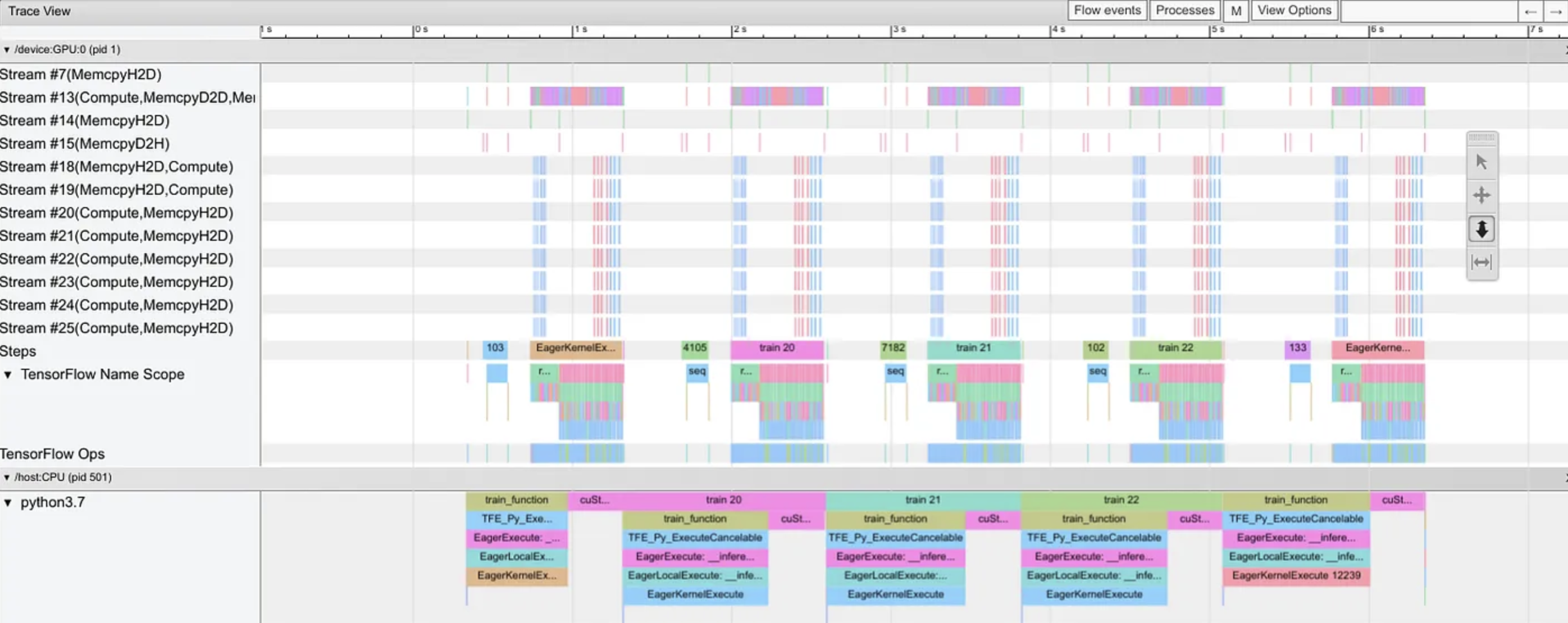](https://mlsysbook.ai/contents/core/training/images/png/tf_profiler.png "Figure 18: GPU Underutilization: Profiling reveals identify data loading as a bottleneck, preventing full GPU utilization during training and increasing overall training time. The gaps in GPU activity indicate the device frequently waits for input data, suggesting optimization of the data pipeline is necessary to maximize computational throughput.")
Figure 18: **GPU Underutilization**: Profiling reveals identify data loading as a bottleneck, preventing full GPU utilization during training and increasing overall training time. The gaps in GPU activity indicate the device frequently waits for input data, suggesting optimization of the data pipeline is necessary to maximize computational throughput.
Identifying these bottlenecks typically involves using profiling tools to analyze the performance of the training system. Tools integrated into machine learning frameworks, such as PyTorch’s `torch.profiler` or TensorFlow’s `tf.data` analysis utilities, can provide detailed insights into where time and resources are being spent during training. By pinpointing the specific stages or operations that are causing delays, practitioners can design targeted optimizations to address these issues effectively.
### System-Level Techniques
After identifying the bottlenecks in a training system, the next step is to implement optimizations at the system level. These optimizations target the underlying hardware, data flow, and resource allocation to improve overall performance and scalability.
One essential technique is profiling training workloads[35](https://mlsysbook.ai/contents/core/training/training.html#fn35)
. Profiling involves collecting detailed metrics about the system’s performance during training, such as computation times, memory usage, and communication overhead. These metrics help reveal inefficiencies, such as imbalanced resource usage or excessive time spent in specific stages of the training pipeline. Profiling tools such as NVIDIA Nsight Systems or TensorFlow Profiler can provide actionable insights, enabling developers to make informed adjustments to their training configurations.
35 **Training Profiling Tools**: NVIDIA Nsight Systems can identify that data loading consumes 20-40% of training time in poorly optimized pipelines, while TensorFlow Profiler reveals GPU utilization rates (optimal: >90%). Intel VTune showed that memory bandwidth often limits performance more than raw compute—typical deep learning workloads achieve only 30-50% of peak FLOPS due to memory bottlenecks.
Leveraging hardware-specific features is another critical aspect of system-level optimization. Modern accelerators, such as GPUs and TPUs, include specialized capabilities that can significantly enhance performance when utilized effectively. For instance, mixed precision training, which uses lower-precision floating-point formats like FP16 or bfloat16 for computations, can dramatically reduce memory usage and improve throughput without sacrificing model accuracy. Similarly, tensor cores in NVIDIA GPUs are designed to accelerate matrix operations, a common computational workload in deep learning, making them ideal for optimizing forward and backward passes.
Data pipeline optimization is also an important consideration at the system level. Ensuring that data is loaded, preprocessed, and delivered to the training devices efficiently can eliminate potential bottlenecks caused by slow data delivery. Techniques such as caching frequently used data, prefetching batches to overlap computation and data loading, and using efficient data storage formats like TFRecord or RecordIO can help maintain a steady flow of data to computational devices.
### Software-Level Techniques
In addition to system-level adjustments, software-level optimizations focus on improving the efficiency of training algorithms and their implementation within machine learning frameworks.
One effective software-level optimization is the use of fused kernels. In traditional implementations, operations like matrix multiplications, activation functions, and gradient calculations are often executed as separate steps. Fused kernels combine these operations into a single optimized routine, reducing the overhead associated with launching multiple operations and improving cache utilization. Many frameworks, such as PyTorch and TensorFlow, automatically apply kernel fusion where possible, but developers can further optimize custom operations by explicitly using libraries like cuBLAS or cuDNN.
Dynamic graph execution is another useful technique for software-level optimization. In frameworks that support dynamic computation graphs, such as PyTorch, the graph of operations is constructed on-the-fly during each training iteration. This flexibility allows for fine-grained optimizations based on the specific inputs and outputs of a given iteration. Dynamic graphs also enable more efficient handling of variable-length sequences, such as those encountered in natural language processing tasks.
Gradient accumulation is an additional strategy that can be implemented at the software level to address memory constraints. Instead of updating model parameters after every batch, gradient accumulation allows the system to compute gradients over multiple smaller batches and update parameters only after aggregating them. This approach effectively increases the batch size without requiring additional memory, enabling training on larger datasets or models.
### Scale-Up Strategies
Scaling techniques aim to extend the capabilities of training systems to handle larger datasets and models by optimizing the training configuration and resource allocation.
One common scaling technique is batch size scaling. Increasing the batch size can reduce the number of synchronization steps required during training, as fewer updates are needed to process the same amount of data. This approach contrasts with the dynamic batching strategies used in inference serving, where the goal is optimizing throughput for variable-length requests rather than training convergence. However, larger batch sizes may introduce challenges, such as slower convergence or reduced generalization. Techniques like learning rate scaling and warmup schedules[36](https://mlsysbook.ai/contents/core/training/training.html#fn36)
can help mitigate these issues, ensuring stable and effective training even with large batches.
36 **Learning Rate Schedules**: Critical for training stability and convergence. Cosine annealing (introduced in 2016) and linear warmup (from BERT 2018) became standard after showing 2-5% accuracy improvements. Large batch training requires linear scaling rule: multiply learning rate by batch size ratio (batch 512 → LR 0.1, batch 4096 → LR 0.8), discovered through extensive experimentation by Facebook and Google teams.
Layer-freezing strategies provide another method for scaling training systems efficiently. In many scenarios, particularly in transfer learning, the lower layers of a model capture general features and do not need frequent updates. By freezing these layers and allowing only the upper layers to train, memory and computational resources can be conserved, enabling the system to focus its efforts on fine-tuning the most critical parts of the model.
While distributed training techniques provide one dimension of scaling, the computational efficiency of individual devices within distributed systems determines overall performance. The optimization techniques and parallelization strategies we have explored achieve their full potential only when executed on hardware architectures designed to maximize throughput for machine learning workloads. This motivates our examination of specialized hardware platforms that accelerate the mathematical operations underlying all training scenarios.
Hardware Acceleration
---------------------
The optimization techniques we have discussed operate within the constraints imposed by underlying hardware architectures. The evolution of specialized machine learning hardware represents an important development in addressing the computational demands of modern training systems. Each hardware architecture, such as GPUs, TPUs, FPGAs, and ASICs, embodies distinct design philosophies and engineering trade-offs that optimize for specific aspects of the training process. These specialized processors have significantly altered the scalability and efficiency constraints of machine learning systems, enabling advances in model complexity and training speed. This hardware evolution builds upon the foundational understanding of ML system design principles established in **[Chapter 2: ML Systems](https://mlsysbook.ai/contents/core/ml_systems/ml_systems.html#sec-ml-systems)
**. We briefly examine the architectural principles, performance characteristics, and practical applications of each hardware type, highlighting their important role in shaping the future capabilities of machine learning training systems.
### GPUs
Machine learning training systems demand immense computational power to process large datasets, perform gradient computations, and update model parameters efficiently. GPUs have emerged as a critical technology to meet these requirements ([Figure 19](https://mlsysbook.ai/contents/core/training/training.html#fig-training-gpus)
), primarily due to their highly parallelized architecture and ability to execute the dense linear algebra operations central to neural network training ([Dally, Keckler, and Kirk 2021](https://mlsysbook.ai/contents/core/training/training.html#ref-dally2021evolution)
).
Dally, William J., Stephen W. Keckler, and David B. Kirk. 2021. “Evolution of the Graphics Processing Unit (GPU).” _IEEE Micro_ 41 (6): 42–51. [https://doi.org/10.1109/mm.2021.3113475](https://doi.org/10.1109/mm.2021.3113475)
.
[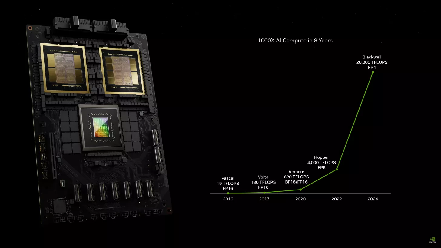](https://mlsysbook.ai/contents/core/training/images/png/acc_gpus.png "Figure 19: GPU Acceleration Trends: Successive GPU generations deliver exponential increases in FLOPS, enabling training of increasingly large and complex machine learning models and driving breakthroughs in areas like natural language processing. These advancements, spanning from pascal to blackwell, showcase the critical role of specialized hardware in overcoming the computational demands of modern AI.")
Figure 19: **GPU Acceleration Trends**: Successive GPU generations deliver exponential increases in FLOPS, enabling training of increasingly large and complex machine learning models and driving breakthroughs in areas like natural language processing. These advancements, spanning from pascal to blackwell, showcase the critical role of specialized hardware in overcoming the computational demands of modern AI.
From the perspective of training pipeline architecture, GPUs address several key bottlenecks. The large number of cores in GPUs allows for simultaneous processing of thousands of matrix multiplications, accelerating the forward and backward passes of training. In systems where data throughput limits GPU utilization, prefetching and caching mechanisms help maintain a steady flow of data. These optimizations, previously discussed in training pipeline design, are critical to unlocking the full potential of GPUs ([Patterson and Hennessy 2021b](https://mlsysbook.ai/contents/core/training/training.html#ref-Patterson2021)
).
———. 2021b. _Computer Organization and Design RISC-v Edition: The Hardware Software Interface_. 2nd ed. San Francisco, CA: Morgan Kaufmann.
37 **NVIDIA NCCL (Collective Communications Library)**: Optimized for multi-GPU communication, NCCL achieves 90-95% of theoretical bandwidth on modern interconnects. On DGX systems with NVLink, NCCL can transfer 600 GB/s between 8 GPUs—50x faster than PCIe—making efficient distributed training possible. It implements optimized AllReduce algorithms that reduce communication from O(n²) to O(n).
38 **GPT-3 Training Scale**: Used 10,000 NVIDIA V100 GPUs for 3-4 months, consuming an estimated 1,287 MWh of energy (roughly equivalent to 120 US homes for a year). The training cost was estimated at $4-12 million (varying by infrastructure and energy costs), demonstrating how specialized hardware and distributed systems enable training at previously impossible scales while highlighting the enormous resource requirements.
In distributed training systems, GPUs enable scalable strategies such as data parallelism and model parallelism. NVIDIA’s ecosystem, including tools like [NCCL](https://developer.nvidia.com/nccl)
[37](https://mlsysbook.ai/contents/core/training/training.html#fn37)
for multi-GPU communication, facilitates efficient parameter synchronization, a frequent challenge in large-scale setups. For example, in training large models like GPT-3[38](https://mlsysbook.ai/contents/core/training/training.html#fn38)
, GPUs were used in tandem with distributed frameworks to split computations across thousands of devices while addressing memory and compute scaling issues ([Brown et al. 2020](https://mlsysbook.ai/contents/core/training/training.html#ref-brown2020language)
).
Hardware-specific features further enhance GPU performance. NVIDIA’s tensor cores[39](https://mlsysbook.ai/contents/core/training/training.html#fn39)
, for instance, are optimized for mixed-precision training, which reduces memory usage while maintaining numerical stability ([Micikevicius et al. 2017](https://mlsysbook.ai/contents/core/training/training.html#ref-micikevicius2017mixed)
). This directly addresses memory constraints, a common bottleneck in training massive models. Combined with software-level optimizations like fused kernels, GPUs deliver substantial speedups in both single-device and multi-device configurations.
39 **Tensor Cores**: Introduced with NVIDIA’s Volta architecture (2017), Tensor Cores deliver 4x speedup for mixed-precision training by performing 4x4 matrix operations in a single clock cycle. The H100’s 4th-gen Tensor Cores achieve 989 TFLOPS for FP16 operations—roughly 6x faster than traditional CUDA cores—enabling training of larger models with the same hardware budget.
Micikevicius, Paulius, Sharan Narang, Jonah Alben, Gregory Diamos, Erich Elsen, David Garcia, Boris Ginsburg, et al. 2017. “Mixed Precision Training.” _arXiv Preprint arXiv:1710.03740_, October. [http://arxiv.org/abs/1710.03740v3](http://arxiv.org/abs/1710.03740v3)
.
A case study that exemplifies the role of GPUs in machine learning training is OpenAI’s use of NVIDIA hardware for large language models. Training GPT-3, with its 175 billion parameters, required distributed processing across thousands of V100 GPUs. The combination of GPU-optimized frameworks, advanced communication protocols, and hardware features enabled OpenAI to achieve this ambitious scale efficiently ([Brown et al. 2020](https://mlsysbook.ai/contents/core/training/training.html#ref-brown2020language)
). The privacy and security implications of such large-scale training—including data governance and model security—are addressed integratedly in **[Chapter 15: Security & Privacy](https://mlsysbook.ai/contents/core/privacy_security/privacy_security.html#sec-security-privacy)
**.
Despite their advantages, GPUs are not without challenges. Effective utilization of GPUs demands careful attention to workload balancing and inter-device communication. Training systems must also consider the cost implications, as GPUs are resource-intensive and require optimized data centers to operate at scale. However, with innovations like [NVLink](https://www.nvidia.com/en-us/data-center/nvlink/)
and [CUDA-X libraries](https://developer.nvidia.com/cuda-zone)
[40](https://mlsysbook.ai/contents/core/training/training.html#fn40)
, these challenges are continually being addressed.
40 **CUDA Programming Model**: Introduced by NVIDIA in 2007, CUDA (Compute Unified Device Architecture) transformed GPUs from graphics processors into general-purpose parallel computing platforms. Unlike CPU programming with 4-16 cores, CUDA enables programming thousands of lightweight threads (32 threads per “warp”). ML frameworks like PyTorch and TensorFlow abstract away CUDA complexity, but understanding concepts like memory coalescing, shared memory, and occupancy remains crucial for optimizing custom ML operations.
GPUs are indispensable for modern machine learning training systems due to their versatility, scalability, and integration with advanced software frameworks. The architectural principles discussed here extend beyond training to influence inference deployment strategies, as detailed in **[Chapter 11: AI Acceleration](https://mlsysbook.ai/contents/core/hw_acceleration/hw_acceleration.html#sec-ai-acceleration)
**, where similar parallelization concepts apply to production environments. By addressing key bottlenecks in computation, memory, and distribution, GPUs play a foundational role in enabling large-scale training pipelines.
GPT-2 GPU Hardware Comparison
Hardware selection significantly impacts GPT-2 training economics and timeline. This comparison shows real-world performance differences.
**Training Throughput (samples/second)**
| | | | | |
| --- | --- | --- | --- | --- |
| V100 (2017) | 90 | 220 | 32GB | $3.06 |
| A100 (2020) | 180 | 450 | 80GB | $4.10 |
| H100 (2022) | 320 | 820 | 80GB | $8.00 |
**Training Time to 50K Steps (8 GPUs)**
* V100: 14 days, cost: approximately $10,252
* A100: 7 days, cost: approximately $6,877
* H100: 3.5 days, cost: approximately $6,720
_Note: Cloud pricing varies significantly and changes frequently by provider._
**Key Hardware-Driven Tradeoffs**
1. Memory capacity enables larger batches: V100’s 32GB limits batch\_size=16, while A100’s 80GB allows batch\_size=32 → faster convergence
2. Tensor Core generations: H100’s 4th-gen Tensor Cores provide 3.7× speedup over V100 for FP16 operations
3. NVLink bandwidth: H100’s 900 GB/s (vs V100’s 300 GB/s) reduces gradient synchronization time by 65%
**Why H100 Wins Despite Higher $/hour**
* Total cost lower due to 4× faster training
* Frees GPUs for other workloads sooner
* Reduced energy consumption (3.5 vs 14 days runtime)
**Hardware Selection Heuristic:** For models like GPT-2 where training runs take days/weeks, newer GPUs with higher throughput typically offer better total cost of ownership despite higher hourly rates. For quick experiments (<1 hour), older GPUs may be more cost-effective.
### TPUs
Tensor Processing Units (TPUs) and other custom accelerators have been purpose-built to address the unique challenges of large-scale machine learning training. Unlike GPUs, which are versatile and serve a wide range of applications, TPUs are specifically optimized for the computational patterns found in deep learning, such as matrix multiplications and convolutional operations ([Jouppi et al. 2017](https://mlsysbook.ai/contents/core/training/training.html#ref-jouppi2017tpu)
). These devices mitigate training bottlenecks by offering high throughput, specialized memory handling, and tight integration with machine learning frameworks.
As illustrated in [Figure 20](https://mlsysbook.ai/contents/core/training/training.html#fig-training-tpus)
, TPUs have undergone significant architectural evolution, with each generation introducing enhancements tailored for increasingly demanding AI workloads. The first-generation TPU, introduced in 2015, was designed for internal inference acceleration. Subsequent iterations have focused on large-scale distributed training, memory optimizations, and efficiency improvements, culminating in the most recent Trillium architecture. These advancements illustrate how domain-specific accelerators continue to push the boundaries of AI performance and efficiency.
[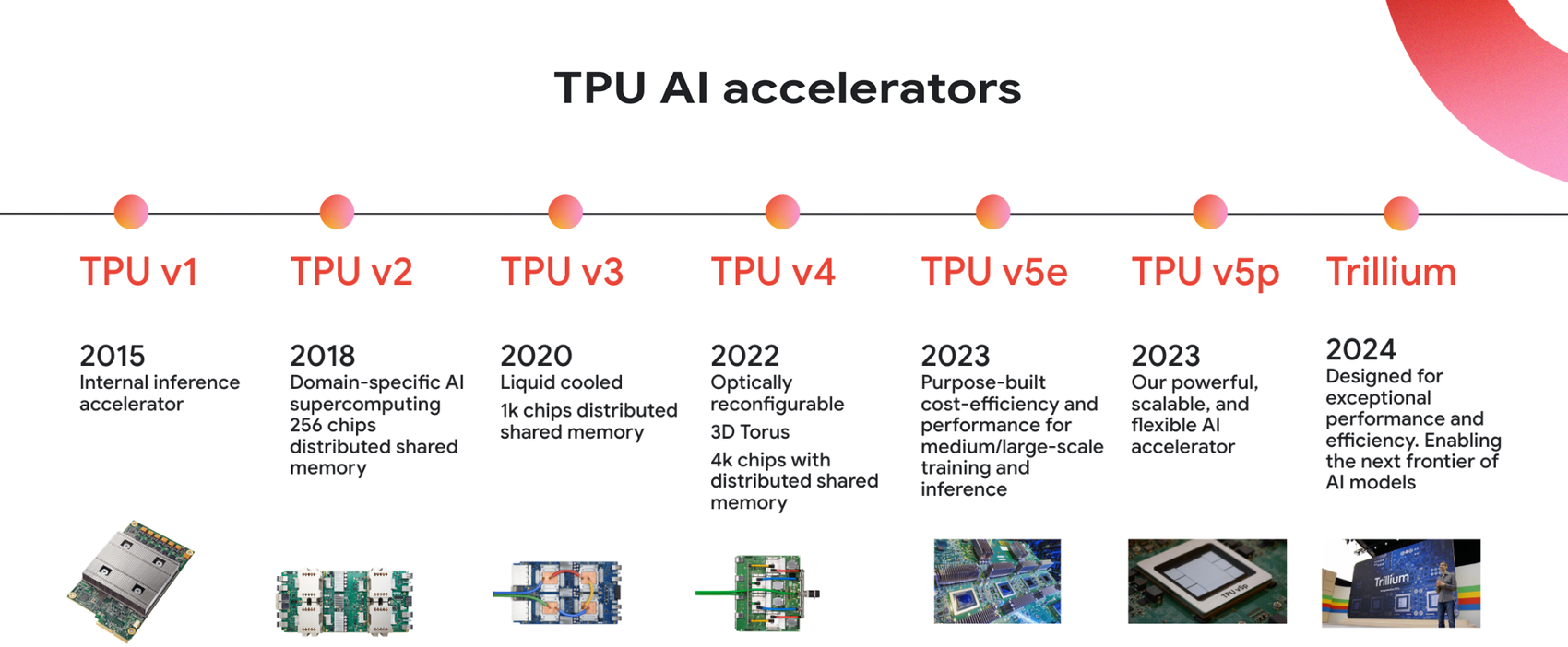](https://mlsysbook.ai/contents/core/training/images/png/acc_tpus.png "Figure 20: TPU Evolution: Successive generations of tensor processing units demonstrate architectural advancements optimized for deep learning workloads, transitioning from inference acceleration to large-scale distributed training and culminating in the trillium architecture. These specialized accelerators address the computational demands of modern AI by enhancing memory handling, increasing throughput, and integrating tightly with machine learning frameworks.")
Figure 20: **TPU Evolution**: Successive generations of tensor processing units demonstrate architectural advancements optimized for deep learning workloads, transitioning from inference acceleration to large-scale distributed training and culminating in the trillium architecture. These specialized accelerators address the computational demands of modern AI by enhancing memory handling, increasing throughput, and integrating tightly with machine learning frameworks.
Machine learning frameworks can achieve substantial gains in training efficiency through purpose-built AI accelerators such as TPUs. However, maximizing these benefits requires careful attention to hardware-aware optimizations, including memory layout, dataflow orchestration, and computational efficiency.
Google developed TPUs with a primary goal: to accelerate machine learning workloads at scale while reducing the energy and infrastructure costs associated with traditional hardware. Their architecture is optimized for tasks that benefit from batch processing, making them particularly effective in distributed training systems where large datasets are split across multiple devices. A key feature of TPUs is their systolic array architecture[41](https://mlsysbook.ai/contents/core/training/training.html#fn41)
, which performs efficient matrix multiplications by streaming data through a network of processing elements. This design minimizes data movement overhead, reducing latency and energy consumption—critical factors for training large-scale models like transformers ([Jouppi et al. 2017](https://mlsysbook.ai/contents/core/training/training.html#ref-jouppi2017tpu)
).
41 **Systolic Array Architecture**: Developed at Carnegie Mellon in 1978, systolic arrays excel at matrix operations by streaming data through a grid of processing elements. Google’s TPU v4 achieves 275 TFLOPS (bfloat16) with ~200W typical power consumption—achieving approximately 1.38 TFLOPS/W efficiency, roughly 2-3x more energy-efficient than comparable GPUs for ML workloads.
Jouppi, Norman P., Cliff Young, Nishant Patil, David Patterson, Gaurav Agrawal, Raminder Bajwa, Sarah Bates, et al. 2017. “In-Datacenter Performance Analysis of a Tensor Processing Unit.” In _Proceedings of the 44th Annual International Symposium on Computer Architecture_, 1–12. ACM. [https://doi.org/10.1145/3079856.3080246](https://doi.org/10.1145/3079856.3080246)
.
Abadi, Martín, Ashish Agarwal, Paul Barham, Eugene Brevdo, Zhifeng Chen, Craig Citro, Greg S. Corrado, et al. 2016. “TensorFlow: Large-Scale Machine Learning on Heterogeneous Distributed Systems.” _arXiv Preprint arXiv:1603.04467_, March. [http://arxiv.org/abs/1603.04467v2](http://arxiv.org/abs/1603.04467v2)
.
From the perspective of training pipeline optimization, TPUs simplify integration with data pipelines in the TensorFlow ecosystem. Features such as the TPU runtime and TensorFlow’s [`tf.data` API](https://www.tensorflow.org/guide/data)
enable seamless preprocessing, caching, and batching of data to feed the accelerators efficiently ([Abadi et al. 2016](https://mlsysbook.ai/contents/core/training/training.html#ref-abadi2016tensorflow)
). TPUs are designed to work in pods—clusters of interconnected TPU devices that allow for massive parallelism. In such setups, TPU pods enable hybrid parallelism strategies by combining data parallelism across devices with model parallelism within devices, addressing memory and compute constraints simultaneously.
TPUs have been instrumental in training large-scale models, such as BERT and T5. For example, Google’s use of TPUs to train BERT demonstrates their ability to handle both the memory-intensive requirements of large transformer models and the synchronization challenges of distributed setups ([Devlin et al. 2018](https://mlsysbook.ai/contents/core/training/training.html#ref-Devlin2019)
). By splitting the model across TPU cores and optimizing communication patterns, Google achieved excellent results while significantly reducing training time compared to traditional hardware.
Devlin, Jacob, Ming-Wei Chang, Kenton Lee, and Kristina Toutanova. 2018. “BERT: Pre-Training of Deep Bidirectional Transformers for Language Understanding,” October, 4171–86. [http://arxiv.org/abs/1810.04805v2](http://arxiv.org/abs/1810.04805v2)
.
Beyond TPUs, custom accelerators such as [AWS Trainium](https://aws.amazon.com/machine-learning/trainium/)
and [Intel Gaudi](https://www.intel.com/content/www/us/en/artificial-intelligence/gaudi-deep-learning.html)
chips are also gaining traction in the machine learning ecosystem. These devices are designed to compete with TPUs by offering similar performance benefits while catering to diverse cloud and on-premise environments. For example, AWS Trainium provides deep integration with the AWS ecosystem, allowing users to seamlessly scale their training pipelines with services like [Amazon SageMaker](https://aws.amazon.com/sagemaker/)
.
While TPUs and custom accelerators excel in throughput and energy efficiency, their specialized nature introduces limitations. The trade-offs between specialized hardware performance and deployment flexibility become particularly important when considering edge deployment scenarios, as explored in **[Chapter 14: On-Device Learning](https://mlsysbook.ai/contents/core/ondevice_learning/ondevice_learning.html#sec-ondevice-learning)
**. TPUs, for example, are tightly coupled with Google’s ecosystem, making them less accessible to practitioners using alternative frameworks. Similarly, the high upfront investment required for TPU pods may deter smaller organizations or those with limited budgets. Despite these challenges, the performance gains offered by custom accelerators make them a compelling choice for large-scale training tasks.
TPUs and custom accelerators address many of the key challenges in machine learning training systems, from handling massive datasets to optimizing distributed training. Their unique architectures and deep integration with specific ecosystems make them powerful tools for organizations seeking to scale their training workflows. As machine learning models and datasets continue to grow, these accelerators are likely to play an increasingly central role in shaping the future of AI training.
### FPGAs
Field-Programmable Gate Arrays (FPGAs) are versatile hardware solutions that allow developers to tailor their architecture for specific machine learning workloads. Unlike GPUs or TPUs, which are designed with fixed architectures, FPGAs can be reconfigured dynamically, offering a unique level of flexibility. This adaptability makes them particularly valuable for applications that require customized optimizations, low-latency processing, or experimentation with novel algorithms.
Microsoft had been exploring the use of FPGAs for a while, as seen in [Figure 21](https://mlsysbook.ai/contents/core/training/training.html#fig-inference-fpgas)
, with one prominent example being [Project Brainwave](https://www.microsoft.com/en-us/research/project/project-brainwave/)
. This initiative uses FPGAs to accelerate machine learning workloads in the Azure cloud. Microsoft chose FPGAs for their ability to provide low-latency inference (not training) while maintaining high throughput. This approach benefits scenarios where real-time predictions are critical, such as search engine queries or language translation services. By integrating FPGAs directly into their data center network[42](https://mlsysbook.ai/contents/core/training/training.html#fn42)
, Microsoft has achieved significant performance gains while minimizing power consumption.
42 **Microsoft FPGA Deployment**: Project Catapult deployed FPGAs across Microsoft’s entire datacenter fleet by 2016, with one FPGA per server (>1 million total). This $1 billion investment improved Bing search latency by 50% and Azure ML inference by 2x, while reducing power consumption by 10-15% through specialized acceleration of specific algorithms.
[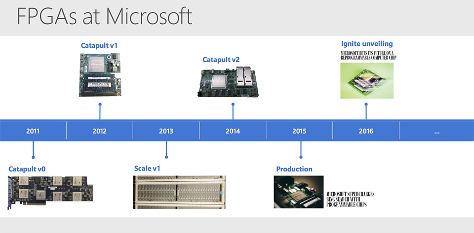](https://mlsysbook.ai/contents/core/training/images/png/acc_fpgas.png "Figure 21: FPGA Evolution for Inference: Microsoft progressively developed field-programmable gate arrays (fpgas) to accelerate machine learning inference in cloud services, shifting from initial project catapult designs to more advanced iterations and ultimately project brainwave. These reconfigurable hardware solutions offer low-latency processing and high throughput, particularly valuable for real-time applications like search and language translation.")
Figure 21: **FPGA Evolution for Inference**: Microsoft progressively developed field-programmable gate arrays (fpgas) to accelerate machine learning inference in cloud services, shifting from initial project catapult designs to more advanced iterations and ultimately project brainwave. These reconfigurable hardware solutions offer low-latency processing and high throughput, particularly valuable for real-time applications like search and language translation.
From a training perspective, FPGAs offer unique advantages in optimizing training pipelines. Their reconfigurability allows them to implement custom dataflow architectures tailored to specific model requirements. While this training-focused customization differs from the inference-oriented FPGA applications more commonly deployed, both approaches use the flexibility that distinguishes FPGAs from fixed-function accelerators. For instance, data preprocessing and augmentation steps, which can often become bottlenecks in GPU-based systems, can be offloaded to FPGAs, freeing up GPUs for core training tasks. FPGAs can be programmed to perform operations such as sparse matrix multiplications, which are common in recommendation systems and graph-based models but are less efficient on traditional accelerators ([Putnam et al. 2014](https://mlsysbook.ai/contents/core/training/training.html#ref-Putnam2014)
).
Putnam, Andrew, Adrian M. Caulfield, Eric S. Chung, Derek Chiou, Kypros Constantinides, John Demme, Hadi Esmaeilzadeh, et al. 2014. “A Reconfigurable Fabric for Accelerating Large-Scale Datacenter Services.” _ACM SIGARCH Computer Architecture News_ 42 (3): 13–24. [https://doi.org/10.1145/2678373.2665678](https://doi.org/10.1145/2678373.2665678)
.
In distributed training systems, FPGAs provide fine-grained control over communication patterns. This control allows developers to optimize inter-device communication and memory access, addressing challenges such as parameter synchronization overheads. For example, FPGAs can be configured to implement custom all-reduce algorithms for gradient aggregation, reducing latency compared to general-purpose hardware.
Despite their benefits, FPGAs come with challenges. Programming FPGAs requires expertise in hardware description languages (HDLs) like Verilog or VHDL, which can be a barrier for many machine learning practitioners. To address this, frameworks like [Xilinx’s Vitis AI](https://www.xilinx.com/products/design-tools/vitis/vitis-ai.html)
and [Intel’s OpenVINO](https://www.intel.com/content/www/us/en/developer/tools/openvino-toolkit/overview.html)
have simplified FPGA programming by providing tools and libraries tailored for AI workloads. However, the learning curve remains steep compared to the well-established ecosystems of GPUs and TPUs.
Microsoft’s use of FPGAs highlights their potential to integrate seamlessly into existing machine learning workflows. This approach demonstrates the versatility of FPGAs, which serve different but complementary roles in training acceleration compared to their more common application in inference optimization, particularly in edge deployments. By incorporating FPGAs into Azure, Microsoft has demonstrated how these devices can complement other accelerators, optimizing end-to-end pipelines for both training and inference. This hybrid approach uses the strengths of FPGAs for specific tasks while relying on GPUs or CPUs for others, creating a balanced and efficient system.
FPGAs offer a compelling solution for machine learning training systems that require customization, low latency, or novel optimizations. While their adoption may be limited by programming complexity, advancements in tooling and real-world implementations like Microsoft’s Project Brainwave demonstrate their growing relevance in the AI hardware ecosystem.
### ASICs
Application-Specific Integrated Circuits (ASICs) represent a class of hardware designed for specific tasks, offering unparalleled efficiency and performance by eschewing the general-purpose flexibility of GPUs or FPGAs. Among the most innovative examples of ASICs for machine learning training is the [Cerebras Wafer-Scale Engine (WSE)](https://www.cerebras.net/)
, as shown in [Figure 22](https://mlsysbook.ai/contents/core/training/training.html#fig-training-wse)
, which stands apart for its unique approach to addressing the computational and memory challenges of training massive machine learning models.
[](https://mlsysbook.ai/contents/core/training/images/png/acc_wse.png "Figure 22: Wafer-Scale Integration: This 300mm silicon wafer contains 2.6 trillion transistors, enabling a single chip to house an entire AI training system and overcome memory bandwidth limitations common in distributed training setups. By integrating massive computational resources onto a single die, the WSE significantly reduces data transfer bottlenecks and accelerates model training for large-scale machine learning applications.")
Figure 22: **Wafer-Scale Integration**: This 300mm silicon wafer contains 2.6 trillion transistors, enabling a single chip to house an entire AI training system and overcome memory bandwidth limitations common in distributed training setups. By integrating massive computational resources onto a single die, the WSE significantly reduces data transfer bottlenecks and accelerates model training for large-scale machine learning applications.
The Cerebras WSE is unlike traditional chips in that it is a single wafer-scale processor, spanning the entire silicon wafer rather than being cut into smaller chips. This architecture enables Cerebras to pack 2.6 trillion transistors and 850,000 cores onto a single device[43](https://mlsysbook.ai/contents/core/training/training.html#fn43)
. These cores are connected via a high-bandwidth, low-latency interconnect, allowing data to move across the chip without the bottlenecks associated with external communication between discrete GPUs or TPUs ([Feldman et al. 2020](https://mlsysbook.ai/contents/core/training/training.html#ref-Feldman2020)
).
43 **Wafer-Scale Engine Specifications**: The WSE-2 (2021) contains 2.6 trillion transistors on a 21cm x 21cm wafer—the largest chip ever manufactured. With 850,000 cores and 40GB on-chip memory, it delivers 15-20x speedup vs. GPU clusters for large language models while consuming 15kW (comparable to 16-20 V100 GPUs but with orders of magnitude less communication overhead).
Feldman, Andrew, Sean Lie, Michael James, et al. 2020. “The Cerebras Wafer-Scale Engine: Opportunities and Challenges of Building an Accelerator at Wafer Scale.” _IEEE Micro_ 40 (2): 20–29. [https://doi.org/10.1109/MM.2020.2975796](https://doi.org/10.1109/MM.2020.2975796)
.
From a machine learning training perspective, the WSE addresses several critical bottlenecks:
1. **Data Movement**: In traditional distributed systems, significant time is spent transferring data between devices. The WSE eliminates this by keeping all computations and memory on a single wafer, drastically reducing communication overhead.
2. **Memory Bandwidth**: The WSE integrates 40 GB of high-speed on-chip memory directly adjacent to its processing cores. This proximity allows for near-instantaneous access to data, overcoming the latency challenges that GPUs often face when accessing off-chip memory.
3. **Scalability**: While traditional distributed systems rely on complex software frameworks to manage multiple devices, the WSE simplifies scaling by consolidating all resources into one massive chip. This design is particularly well-suited for training large language models and other deep learning architectures that require significant parallelism.
A key example of Cerebras’ impact is its application in natural language processing. Organizations using the WSE have demonstrated substantial speedups in training transformer models, which are notoriously compute-intensive due to their reliance on attention mechanisms. The responsible deployment of such powerful training capabilities—including considerations of energy consumption, accessibility, and societal impact—is explored in **[Chapter 17: Responsible AI](https://mlsysbook.ai/contents/core/responsible_ai/responsible_ai.html#sec-responsible-ai)
**. By leveraging the chip’s massive parallelism and memory bandwidth, training times for models like BERT have been significantly reduced compared to GPU-based systems ([Brown et al. 2020](https://mlsysbook.ai/contents/core/training/training.html#ref-brown2020language)
).
Brown, Tom B., Benjamin Mann, Nick Ryder, Melanie Subbiah, Jared Kaplan, Prafulla Dhariwal, Arvind Neelakantan, et al. 2020. “Language Models Are Few-Shot Learners.” _Advances in Neural Information Processing Systems (NeurIPS)_ 33: 1877–1901.
However, the Cerebras WSE also comes with limitations. Its single-chip design is optimized for specific use cases, such as dense matrix computations in deep learning, but may not be as versatile as multi-purpose hardware like GPUs or FPGAs. The cost of acquiring and integrating such a specialized device can be prohibitive for smaller organizations or those with diverse workloads.
Cerebras’ strategy of targeting the largest models aligns with previously discussed trends, such as the growing emphasis on scaling techniques and hybrid parallelism strategies. The WSE’s unique design addresses challenges like memory bottlenecks and inter-device communication overhead, making it a pioneering solution for next-generation AI workloads.
The Cerebras Wafer-Scale Engine exemplifies how ASICs can push the boundaries of what is possible in machine learning training. By addressing key bottlenecks in computation and data movement, the WSE offers a glimpse into the future of specialized hardware for AI, where the integration of highly optimized, task-specific architectures unlocks unprecedented performance.
Fallacies and Pitfalls
----------------------
Training represents the most computationally intensive phase of machine learning system development, where complex optimization algorithms, distributed computing challenges, and resource management constraints intersect. The scale and complexity of modern training workloads create numerous opportunities for misconceptions about performance optimization, resource utilization, and system design choices.
**Fallacy:** _Training larger models always yields better performance._
This widespread belief drives teams to continuously scale model size without considering the relationship between model capacity and available data. While larger models can capture more complex patterns, they also require exponentially more data and computation to train effectively. Beyond certain thresholds, increasing model size leads to overfitting on limited datasets, diminishing returns in performance improvements, and unsustainable computational costs. Effective training requires matching model capacity to data availability and computational resources rather than pursuing size for its own sake.
**Pitfall:** _Assuming that distributed training automatically accelerates model development._
Many practitioners expect that adding more devices will proportionally reduce training time without considering communication overhead and synchronization costs. Distributed training introduces coordination complexity, gradient aggregation bottlenecks, and potential convergence issues that can actually slow down training. Small models or datasets might train faster on single devices than distributed systems due to communication overhead. Successful distributed training requires careful analysis of model size, batch size requirements, and communication patterns to achieve actual speedup benefits.
**Fallacy:** _Learning rate schedules that work for small models apply directly to large-scale training._
This misconception assumes that hyperparameters, particularly learning rates, scale linearly with model size or dataset size. Large-scale training often requires different optimization dynamics due to gradient noise characteristics, batch size effects, and convergence behavior changes. Learning rate schedules optimized for small-scale experiments frequently cause instability or poor convergence when applied to distributed training scenarios. Effective large-scale training requires hyperparameter adaptation specific to the scale and distributed nature of the training environment.
**Pitfall:** _Neglecting training reproducibility and experimental tracking._
Under pressure to achieve quick results, teams often sacrifice training reproducibility by using random seeds inconsistently, failing to track hyperparameters, or running experiments without proper versioning. This approach makes it impossible to reproduce successful results, compare experiments fairly, or debug training failures. Complex distributed training setups amplify these issues, where subtle differences in device configuration, data loading order, or software versions can create significant result variations. Systematic experiment tracking and reproducibility practices are essential engineering disciplines, not optional overhead.
**Pitfall:** _Underestimating infrastructure complexity and failure modes in distributed training systems._
Many teams approach distributed training as a straightforward scaling exercise without adequately planning for the infrastructure challenges that emerge at scale. Distributed training systems introduce complex failure modes including node failures, network partitions, memory pressure from unbalanced load distribution, and synchronization deadlocks that can cause entire training runs to fail hours or days into execution. Hardware heterogeneity across training clusters creates performance imbalances where slower nodes become bottlenecks, while network topology and bandwidth limitations can make communication costs dominate computation time. Effective distributed training requires robust checkpoint and recovery mechanisms, load balancing strategies, health monitoring systems, and fallback procedures for handling partial failures. The infrastructure must also account for dynamic resource allocation, spot instance interruptions in cloud environments, and the operational complexity of maintaining consistent software environments across distributed workers.
Summary
-------
Training represents the computational heart of machine learning systems, where mathematical algorithms, memory management strategies, and distributed computing architectures converge to transform data into intelligent models. Throughout this chapter, we have seen how the seemingly simple concept of iterative parameter optimization requires careful engineering solutions to handle the scale and complexity of modern machine learning workloads. The operations of forward and backward propagation become orchestrations of matrix operations, memory allocations, and gradient computations that must be carefully balanced against hardware constraints and performance requirements.
Our exploration from single-device training to distributed systems demonstrates how computational bottlenecks drive architectural innovation rather than simply limiting capabilities. Data parallelism enables scaling across multiple devices by distributing training examples, while model parallelism addresses memory limitations by partitioning model parameters across hardware resources. Advanced techniques like gradient accumulation, mixed precision training, and pipeline parallelism showcase how training systems can optimize memory usage, computational throughput, and convergence stability simultaneously. The interplay between these strategies reveals that effective training system design requires deep understanding of both algorithmic properties and hardware characteristics to achieve optimal resource utilization.
This co-design principle—where algorithms, software frameworks, and hardware architectures evolve together—shapes modern training infrastructure. Matrix operation patterns drove GPU Tensor Core development, which frameworks exposed through mixed-precision APIs, enabling algorithmic techniques like FP16 training that further influenced next-generation hardware design. Understanding this feedback loop between computational requirements and system capabilities enables practitioners to make informed architectural decisions that leverage the full potential of modern training systems.
The training optimizations explored throughout this chapter provide the foundation for the model-level efficiency techniques and deployment strategies examined in subsequent chapters. These systems principles extend naturally from training infrastructure to production inference systems, demonstrating how the engineering insights gained from optimizing training workflows inform the broader machine learning system lifecycle.
Key Takeaways
* Training efficiency depends on optimizing the entire pipeline from data loading through gradient computation and parameter updates
* Distributed training strategies must balance communication overhead against computational parallelism to achieve scaling benefits
* Memory management techniques like gradient checkpointing and mixed precision are essential for training large models within hardware constraints
* Successful training systems require co-design of algorithms, software frameworks, and hardware architectures
These principles and techniques provide the foundation for understanding how model optimization, hardware acceleration, and deployment strategies build upon training infrastructure to create complete machine learning systems. As models continue growing in size and complexity, these training techniques become increasingly critical for making advanced AI capabilities accessible and practical across diverse application domains and computational environments.
Self-Check Answers
------------------
**Self-Check: Answer 1.1**
1. **Which of the following best describes the primary computational challenge during the training phase of machine learning systems?**
1. Limited data availability
2. Lack of algorithmic frameworks
3. High memory and computational requirements
4. Insufficient model interpretability
_Answer_: The correct answer is C. High memory and computational requirements. Training involves models with billions of parameters, requiring extensive memory and computational resources.
_Learning Objective_: Understand the primary computational challenges in the training phase of ML systems.
2. **Explain how the modular system architectures and data pipelines established in earlier chapters support the training phase in machine learning systems.**
_Answer_: Modular system architectures enable distributed training orchestration, while engineered data pipelines provide continuous streams of training samples. This integration supports efficient training by ensuring scalable and reliable data flow and computation.
_Learning Objective_: Understand the role of system components in supporting the training phase of ML systems.
3. **What is a key benefit of using different numerical precisions during training?**
1. Increased model interpretability
2. Improved algorithmic complexity
3. Enhanced data privacy
4. Reduced training time and memory usage
_Answer_: The correct answer is D. Reduced training time and memory usage. Using lower precision for certain operations can reduce memory requirements and increase computational speed while maintaining training stability.
_Learning Objective_: Understand the benefits of precision optimization in ML training systems.
4. **True or False: The training phase in ML systems is less computationally demanding than the deployment phase.**
_Answer_: False. The training phase is the most computationally demanding part of ML systems, requiring extensive resources for optimization and model refinement.
_Learning Objective_: Recognize the computational demands of the training phase compared to other phases.
5. **Consider a scenario where you are tasked with training a model similar to GPT-2. What are some system design considerations you must address to handle the computational demands?**
_Answer_: You must consider memory hierarchy management, efficient inter-node communication, and resource allocation strategies. Additionally, leveraging distributed training and specialized hardware like GPUs for matrix operations is crucial.
_Learning Objective_: Identify system design considerations for handling computational demands in training large-scale models.
[← Back to Questions](https://mlsysbook.ai/contents/core/training/training.html#quiz-question-sec-ai-training-training-systems-evolution-architecture-0293)
**Self-Check: Answer 1.2**
1. **Which of the following characteristics is NOT typical of machine learning training systems?**
1. Extreme computational intensity
2. Substantial memory pressure
3. Low-latency prediction serving
4. Complex data dependencies
_Answer_: The correct answer is C. Low-latency prediction serving. Training systems focus on iterative optimization, not low-latency serving, which is a characteristic of inference systems.
_Learning Objective_: Differentiate between the demands of training and inference systems.
2. **True or False: High-performance computing systems are fully optimized for the unique demands of machine learning training.**
_Answer_: False. HPC systems are optimized for dense, floating-point heavy computations but do not fully address the dynamic memory and synchronization requirements of ML training.
_Learning Objective_: Understand the limitations of traditional HPC systems in the context of ML training.
3. **Explain why modern machine learning training systems require specialized hardware features.**
_Answer_: Modern ML training systems require specialized hardware to handle the intensive parameter updates, complex memory access patterns, and coordinated distributed computation inherent in neural network training. For example, NVIDIA GPUs and Google TPUs are designed to optimize these tasks, providing the necessary computational power and efficiency. This is important because traditional systems cannot meet these demands effectively.
_Learning Objective_: Understand the necessity of specialized hardware in training systems.
4. **Order the following computing eras by their introduction: (1) Mainframe, (2) High-Performance Computing, (3) Warehouse-Scale Computing, (4) AI Hypercomputing.**
_Answer_: The correct order is: (1) Mainframe, (2) High-Performance Computing, (3) Warehouse-Scale Computing, (4) AI Hypercomputing. This sequence reflects the historical progression of computing systems adapting to increasing workload demands.
_Learning Objective_: Understand the historical evolution of computing systems relevant to ML training.
5. **Consider a scenario where you are designing a training system for a large neural network. What trade-offs would you consider between computational intensity and memory usage?**
_Answer_: When designing a training system for a large neural network, trade-offs between computational intensity and memory usage include balancing the need for fast computations with the ability to store large model parameters and activations. For example, using GPUs can provide significant computational power but may require optimizing memory usage through techniques like mixed-precision training. This is important because efficient resource management directly impacts training speed and cost.
_Learning Objective_: Analyze trade-offs in training system design for large neural networks.
[← Back to Questions](https://mlsysbook.ai/contents/core/training/training.html#quiz-question-sec-ai-training-training-systems-45a3)
**Self-Check: Answer 1.3**
1. **Which of the following operations is most computationally dominant in neural network training?**
1. Matrix-vector multiplication
2. Matrix-matrix multiplication
3. Element-wise activation functions
4. Batch normalization
_Answer_: The correct answer is B. Matrix-matrix multiplication. This is correct because matrix-matrix multiplication accounts for the majority of computational workload during both forward and backward passes in neural network training.
_Learning Objective_: Understand the computational dominance of matrix-matrix multiplication in neural network training.
2. **Explain how the choice of activation function can impact system performance in neural network training.**
_Answer_: Activation functions like ReLU are computationally efficient and introduce beneficial sparsity, reducing memory and computation needs compared to functions like sigmoid, which require expensive exponential calculations. This impacts system performance by affecting training speed and hardware utilization. For example, ReLU’s simplicity allows for faster execution on GPUs, while sigmoid’s computational cost can slow down training.
_Learning Objective_: Analyze the impact of activation function choice on system performance and computational efficiency.
3. **Order the following steps in the backpropagation process: (1) Compute gradients, (2) Forward pass, (3) Update parameters.**
_Answer_: The correct order is: (2) Forward pass, (1) Compute gradients, (3) Update parameters. During backpropagation, the forward pass calculates activations, gradients are computed using these activations, and parameters are updated using the computed gradients.
_Learning Objective_: Understand the sequence of operations in the backpropagation process.
4. **What is a primary system-level challenge when using advanced optimization algorithms like Adam?**
1. High computational intensity
2. Limited convergence speed
3. Increased memory overhead
4. Poor hardware utilization
_Answer_: The correct answer is C. Increased memory overhead. Advanced optimizers like Adam require storing additional state information, which increases memory requirements compared to simpler algorithms like SGD.
_Learning Objective_: Identify system-level challenges associated with using advanced optimization algorithms.
5. **Consider a scenario where you are designing a training system for a large neural network. What trade-offs would you consider when selecting an optimization algorithm?**
_Answer_: When selecting an optimization algorithm, consider trade-offs between memory usage, convergence speed, and computational efficiency. For example, Adam offers faster convergence but requires more memory, while SGD uses less memory but may converge more slowly. The choice depends on available hardware resources and the specific training requirements.
_Learning Objective_: Evaluate trade-offs in optimization algorithm selection for system design.
[← Back to Questions](https://mlsysbook.ai/contents/core/training/training.html#quiz-question-sec-ai-training-mathematical-foundations-71a8)
**Self-Check: Answer 1.4**
1. **Which component of the pipeline architecture is primarily responsible for transforming raw data into a format suitable for model training?**
1. Data Pipeline
2. Training Loop
3. Evaluation Pipeline
4. Optimizer
_Answer_: The correct answer is A. Data Pipeline. This component manages the ingestion, preprocessing, and batching of data for training. The other components focus on different aspects of the training process.
_Learning Objective_: Understand the role of the data pipeline in preparing data for training.
2. **Explain how the integration of the data pipeline, training loop, and evaluation pipeline contributes to the efficiency of an ML training system.**
_Answer_: The integration ensures that data preparation overlaps with computation, minimizing idle time. The evaluation pipeline provides feedback that informs adjustments to the model, optimizing the training process. This coordination maximizes resource utilization and maintains a continuous flow of data and computations.
_Learning Objective_: Analyze the benefits of integrating different pipeline components in a training system.
3. **True or False: The evaluation pipeline operates independently of the training loop and does not impact the training process.**
_Answer_: False. The evaluation pipeline provides feedback on model performance, which is crucial for guiding the training process and making necessary adjustments.
_Learning Objective_: Recognize the interdependence of pipeline components in ML systems.
4. **The throughput of preprocessing operations can be expressed mathematically as: \_\_\_\_.**
_Answer_: T\_preprocessing = N\_workers / t\_transform. This equation captures the relationship between the number of parallel processing threads and the time required for each transformation operation.
_Learning Objective_: Recall the mathematical expression for preprocessing throughput.
5. **Order the following stages in the data pipeline: (1) Batching, (2) Format Conversion, (3) Processing.**
_Answer_: The correct order is: (2) Format Conversion, (3) Processing, (1) Batching. Data is first converted into a standard format, then processed, and finally organized into batches.
_Learning Objective_: Understand the sequence of operations in the data pipeline.
[← Back to Questions](https://mlsysbook.ai/contents/core/training/training.html#quiz-question-sec-ai-training-pipeline-architecture-622a)
**Self-Check: Answer 1.5**
1. **Which optimization technique is primarily used to address data movement latency in ML training pipelines?**
1. Mixed-Precision Training
2. Gradient Accumulation
3. Activation Checkpointing
4. Prefetching & Pipeline Overlapping
_Answer_: The correct answer is D. Prefetching & Pipeline Overlapping. This technique addresses data movement latency by coordinating data transfer with computation to maintain a consistent flow of data.
_Learning Objective_: Understand which optimization techniques address specific bottlenecks in training pipelines.
2. **Explain how mixed-precision training improves both computational throughput and memory usage in ML systems.**
_Answer_: Mixed-precision training uses reduced precision formats like FP16 to decrease memory usage and increase computational speed. Modern hardware, such as GPUs with Tensor Cores, is optimized for these operations, allowing faster execution and larger batch sizes while maintaining model accuracy through FP32 master weights.
_Learning Objective_: Analyze the benefits of mixed-precision training in terms of computational efficiency and memory optimization.
3. **Order the following steps in the systematic optimization framework: (1) Select techniques, (2) Profile bottlenecks, (3) Compose solutions.**
_Answer_: The correct order is: (2) Profile bottlenecks, (1) Select techniques, (3) Compose solutions. Profiling identifies bottlenecks, selection matches techniques to constraints, and composition combines techniques for cumulative benefits.
_Learning Objective_: Understand the systematic approach to optimizing ML training pipelines.
4. **True or False: Activation checkpointing primarily aims to reduce computational overhead during training.**
_Answer_: False. Activation checkpointing primarily aims to reduce memory usage by recomputing activations on demand, trading off increased computational time for memory savings.
_Learning Objective_: Clarify misconceptions about the purpose and trade-offs of activation checkpointing.
5. **In a production system with limited memory but high computational capacity, which optimization techniques would you prioritize and why?**
_Answer_: In such a system, prioritizing activation checkpointing and gradient accumulation would be beneficial. Activation checkpointing reduces memory usage by recomputing activations, and gradient accumulation allows larger effective batch sizes without exceeding memory limits. These techniques leverage high computational capacity to manage memory constraints.
_Learning Objective_: Evaluate and prioritize optimization techniques based on specific system constraints and capabilities.
[← Back to Questions](https://mlsysbook.ai/contents/core/training/training.html#quiz-question-sec-ai-training-pipeline-optimizations-3397)
**Self-Check: Answer 1.6**
1. **What is the primary reason for transitioning from single-machine to distributed training in machine learning systems?**
1. To reduce the cost of training
2. To avoid using GPUs
3. To simplify the training process
4. To manage increasing model complexity and dataset sizes
_Answer_: The correct answer is D. To manage increasing model complexity and dataset sizes. Distributed training allows for scaling computational resources to handle large models and datasets that exceed the capacity of a single machine.
_Learning Objective_: Understand the motivation for distributed training in machine learning systems.
2. **Explain the trade-offs between data parallelism and model parallelism in distributed training systems.**
_Answer_: Data parallelism distributes datasets across devices, allowing each device to train a full model copy, which is efficient for large datasets but limited by model size. Model parallelism splits the model across devices, suitable for large models but introduces communication overhead and complexity. The choice depends on model size, dataset size, and available resources.
_Learning Objective_: Analyze the trade-offs between different parallelism strategies in distributed systems.
3. **True or False: In distributed training, communication overhead is a minor concern and does not significantly impact system performance.**
_Answer_: False. Communication overhead is a major concern in distributed training, as it can significantly impact system performance, especially when synchronizing gradients across multiple devices.
_Learning Objective_: Understand the impact of communication overhead on distributed training performance.
4. **Order the following stages in the transition from single-GPU to multi-node distributed training: (1) Optimize single-GPU performance, (2) Scale to multiple GPUs within a node, (3) Move to multi-node distributed training.**
_Answer_: The correct order is: (1) Optimize single-GPU performance, (2) Scale to multiple GPUs within a node, (3) Move to multi-node distributed training. This progression ensures efficient resource utilization at each stage before adding complexity.
_Learning Objective_: Understand the logical progression in scaling machine learning training from single-GPU to distributed systems.
[← Back to Questions](https://mlsysbook.ai/contents/core/training/training.html#quiz-question-sec-ai-training-distributed-systems-8fe8)
Back to top
---
# ML Systems Textbook
Model Optimizations
===================
_DALL·E 3 Prompt: Illustration of a neural network model represented as a busy construction site, with a diverse group of construction workers, both male and female, of various ethnicities, labeled as ‘pruning’, ‘quantization’, and ‘sparsity’. They are working together to make the neural network more efficient and smaller, while maintaining high accuracy. The ‘pruning’ worker, a Hispanic female, is cutting unnecessary connections from the middle of the network. The ‘quantization’ worker, a Caucasian male, is adjusting or tweaking the weights all over the place. The ‘sparsity’ worker, an African female, is removing unnecessary nodes to shrink the model. Construction trucks and cranes are in the background, assisting the workers in their tasks. The neural network is visually transforming from a complex and large structure to a more streamlined and smaller one._

Purpose
-------
_How does the mismatch between research-optimized models and production deployment constraints create critical engineering challenges in machine learning systems?_
Machine learning research prioritizes accuracy above all considerations, producing models with remarkable performance that cannot deploy where needed most: resource-constrained mobile devices, cost-sensitive cloud environments, or latency-critical edge applications. Model optimization bridges theoretical capability and practical deployment, transforming computationally intensive research models into efficient systems preserving performance while meeting stringent constraints on memory, energy, latency, and cost. Without systematic optimization techniques, advanced AI capabilities remain trapped in research laboratories. Understanding optimization principles enables engineers to democratize AI capabilities by making sophisticated models accessible across diverse deployment contexts, from billion-parameter language models running on mobile devices to embedded sensors.
Learning Objectives
* Compare model optimization techniques including pruning, quantization, knowledge distillation, and neural architecture search in terms of their mechanisms and applications
* Evaluate trade-offs between numerical precision levels and their effects on model accuracy, energy consumption, and hardware compatibility
* Apply the tripartite optimization framework (model representation, numerical precision, architectural efficiency) to design deployment strategies for specific hardware constraints
* Analyze how hardware-aware design principles influence model architecture decisions and computational efficiency across different deployment platforms
* Implement sparsity exploitation and dynamic computation techniques to improve inference performance while managing accuracy preservation
* Design integrated optimization pipelines that combine multiple techniques to achieve specific deployment objectives within resource constraints
* Assess automated optimization approaches and their role in discovering novel optimization strategies beyond manual tuning
Model Optimization Fundamentals
-------------------------------
Successful deployment of machine learning systems requires addressing the tension between model sophistication and computational feasibility. Contemporary research in machine learning has produced increasingly powerful models whose resource demands often exceed the practical constraints of real-world deployment environments. This represents the classic engineering challenge of translating theoretical advances into viable systems, affecting the accessibility and scalability of machine learning applications.
The magnitude of this resource gap is substantial and multifaceted. State-of-the-art language models may require several hundred gigabytes of memory for full-precision parameter storage ([Brown et al. 2020](https://mlsysbook.ai/contents/core/optimizations/optimizations.html#ref-brown2020gpt3)
; [Chowdhery et al. 2022](https://mlsysbook.ai/contents/core/optimizations/optimizations.html#ref-chowdhery2022palm)
), while target deployment platforms such as mobile devices typically provide only a few gigabytes of available memory. This disparity extends beyond memory constraints to encompass computational throughput, energy consumption, and latency requirements. The challenge is further compounded by the heterogeneous nature of deployment environments, each imposing distinct constraints and performance requirements.
Brown, Tom B., Benjamin Mann, Nick Ryder, Melanie Subbiah, Jared Kaplan, Prafulla Dhariwal, Arvind Neelakantan, et al. 2020. “Language Models Are Few-Shot Learners.” _Advances in Neural Information Processing Systems_ 33: 1877–1901.
Chowdhery, Aakanksha, Sharan Narang, Jacob Devlin, Maarten Bosma, Gaurav Mishra, Adam Roberts, Paul Barham, et al. 2022. “PaLM: Scaling Language Modeling with Pathways.” _arXiv Preprint arXiv:2204.02311_, April. [http://arxiv.org/abs/2204.02311v5](http://arxiv.org/abs/2204.02311v5)
.
Production machine learning systems operate within a complex optimization landscape characterized by multiple, often conflicting, performance objectives. Real-time applications impose strict latency bounds, mobile deployments require energy efficiency to preserve battery life, embedded systems must operate within thermal constraints, and cloud services demand cost-effective resource utilization at scale. These constraints collectively define a multi-objective optimization problem that requires systematic approaches to achieve satisfactory solutions across all relevant performance dimensions.
**Definition:** Model Optimization
**_Model Optimization_** is the systematic transformation of machine learning models to maximize _computational efficiency_ while preserving _task performance_, enabling deployment across _diverse hardware constraints_.
The engineering discipline of model optimization has evolved to address these challenges through systematic methodologies that integrate algorithmic innovation with hardware-aware design principles. Effective optimization strategies require deep understanding of the interactions between model architecture, numerical precision, computational patterns, and target hardware characteristics. This interdisciplinary approach transforms optimization from an ad hoc collection of techniques into a principled engineering discipline guided by theoretical foundations and empirical validation.
This chapter establishes a comprehensive theoretical and practical framework for model optimization organized around three interconnected dimensions: structural efficiency in model representation, numerical efficiency through precision optimization, and computational efficiency via hardware-aware implementation. Through this framework, we examine how established techniques such as quantization achieve memory reduction and inference acceleration, how pruning methods eliminate parameter redundancy while preserving model accuracy, and how knowledge distillation enables capability transfer from complex models to efficient architectures. The overarching objective transcends simple performance metrics to enable the deployment of sophisticated machine learning capabilities across the complete spectrum of computational environments and application domains.
**Self-Check: Question 1.1**
1. Which of the following best describes the primary goal of model optimization in machine learning systems?
1. Maximize model accuracy regardless of resource constraints.
2. Reduce the size of the model to the smallest possible footprint.
3. Achieve efficient execution in target environments while maintaining accuracy and functionality.
4. Increase the complexity of the model to improve performance.
2. Explain how model optimization techniques like quantization and pruning contribute to efficient deployment of machine learning models.
3. What is a common challenge when deploying sophisticated machine learning models on mobile devices?
1. Excessive computational throughput
2. Unlimited thermal constraints
3. High latency requirements
4. Limited memory and energy resources
4. True or False: Model optimization only focuses on reducing the computational complexity of machine learning models.
5. In a production system, what trade-offs might you consider when implementing model optimization techniques?
[See Answers →](https://mlsysbook.ai/contents/core/optimizations/optimizations.html#quiz-answer-sec-model-optimizations-model-optimization-fundamentals-064e)
Optimization Framework
----------------------
The optimization process operates through three interconnected dimensions that bridge software algorithms and hardware execution, as illustrated in [Figure 1](https://mlsysbook.ai/contents/core/optimizations/optimizations.html#fig-3-sections)
. Understanding these dimensions and their relationships provides the conceptual foundation for all techniques explored in this chapter.
[](https://mlsysbook.ai/contents/core/optimizations/b90a96a6d4772b4b8898ad11c262e3e7ea987b3d.svg "Figure 1: Optimization Stack: Model optimization progresses through three layers (efficient model representation, efficient numerics representation, and efficient hardware implementation), each addressing distinct aspects of system performance and resource utilization. These layers allow structured trade-offs between model accuracy, computational cost, and memory footprint to meet the demands of different deployment environments.")
Figure 1: **Optimization Stack**: Model optimization progresses through three layers (efficient model representation, efficient numerics representation, and efficient hardware implementation), each addressing distinct aspects of system performance and resource utilization. These layers allow structured trade-offs between model accuracy, computational cost, and memory footprint to meet the demands of different deployment environments.
Understanding these layer interactions reveals the systematic nature of optimization engineering. Model representation techniques (pruning, distillation, structured approximations) reduce computational complexity while creating opportunities for numerical precision optimization. Quantization and reduced-precision arithmetic exploit hardware capabilities for faster execution, while architectural efficiency techniques align computation patterns with processor designs. Software optimizations establish the foundation for hardware acceleration by creating structured, predictable workloads that specialized processors can execute efficiently.
This chapter examines each optimization layer through an engineering lens, providing specific algorithms for quantization (post-training and quantization-aware training), pruning strategies (magnitude-based, structured, and dynamic), and distillation procedures (temperature scaling, feature transfer). We explore how these techniques combine synergistically and how their effectiveness depends on target hardware characteristics. The framework guides systematic optimization decisions, ensuring that model transformations align with deployment constraints while preserving essential capabilities.
This chapter transforms the efficiency concepts from earlier foundations into actionable engineering practices through systematic application of optimization principles. Mastery of quantization, pruning, and distillation techniques provides practitioners with the essential tools for deploying sophisticated machine learning models across diverse computational environments. The optimization framework presented bridges the gap between theoretical model capabilities and practical deployment requirements, enabling machine learning systems that deliver both performance and efficiency in real-world applications.
**Self-Check: Question 1.2**
1. Which of the following layers in the optimization stack primarily focuses on aligning computation patterns with processor designs?
1. Efficient Model Representation
2. Efficient Numerics Representation
3. Efficient Data Handling
4. Efficient Hardware Implementation
2. Explain how model representation techniques such as pruning and distillation can create opportunities for numerical precision optimization.
3. In the context of the optimization framework, what is the primary benefit of using quantization techniques?
1. Increasing model accuracy
2. Reducing computational cost
3. Enhancing data privacy
4. Improving data collection
4. True or False: The optimization framework’s effectiveness is independent of the target hardware characteristics.
[See Answers →](https://mlsysbook.ai/contents/core/optimizations/optimizations.html#quiz-answer-sec-model-optimizations-optimization-framework-1c8e)
Deployment Context
------------------
Machine learning models operate as part of larger systems with complex constraints, dependencies, and trade-offs. Model optimization cannot be treated as a purely algorithmic problem; it must be viewed as a systems-level challenge that considers computational efficiency, scalability, deployment feasibility, and overall system performance. Operational principles from **[Chapter 13: ML Operations](https://mlsysbook.ai/contents/core/ops/ops.html#sec-ml-operations)
** provide the foundation for understanding the systems perspective on model optimization, highlighting why optimization is important, the key constraints that drive optimization efforts, and the principles that define an effective optimization strategy.
### Practical Deployment
Modern machine learning models often achieve impressive accuracy on benchmark datasets, but making them practical for real-world use is far from trivial. Machine learning systems operate under computational, memory, latency, and energy constraints that significantly impact both training and inference ([Choudhary et al. 2020](https://mlsysbook.ai/contents/core/optimizations/optimizations.html#ref-choudhary2020comprehensive)
). Models that perform well in research settings may prove impractical when integrated into broader systems, regardless of deployment context including cloud environments, smartphone integration, or microcontroller implementation.
Choudhary, Tejalal, Vipul Mishra, Anurag Goswami, and Jagannathan Sarangapani. 2020. “A Comprehensive Survey on Model Compression and Acceleration.” _Artificial Intelligence Review_ 53 (7): 5113–55. [https://doi.org/10.1007/s10462-020-09816-7](https://doi.org/10.1007/s10462-020-09816-7)
.
1 **Microcontroller Constraints**: Arduino Uno has 2KB SRAM vs. 32KB flash storage. ARM Cortex-M4 implementations typically have 256KB flash, 64KB RAM, running at up to 168MHz vs. modern GPUs with 3000+ MHz clocks and 16-80GB memory, representing a 10,000x+ resource gap.
Beyond these deployment complexities, real-world feasibility encompasses efficiency in training, storage, and execution rather than accuracy alone.[1](https://mlsysbook.ai/contents/core/optimizations/optimizations.html#fn1)
Efficiency requirements manifest differently across deployment contexts. In large-scale cloud ML settings, optimizing models helps minimize training time, computational cost, and power consumption, making large-scale AI workloads more efficient ([Dean, Patterson, and Young 2018](https://mlsysbook.ai/contents/core/optimizations/optimizations.html#ref-dean2018new)
). In contrast, edge ML[2](https://mlsysbook.ai/contents/core/optimizations/optimizations.html#fn2)
requires models to run with limited compute resources, necessitating optimizations that reduce memory footprint and computational complexity. Mobile ML introduces additional constraints, such as battery life and real-time responsiveness, while tiny ML[3](https://mlsysbook.ai/contents/core/optimizations/optimizations.html#fn3)
pushes efficiency to the extreme, requiring models to fit within the memory and processing limits of ultra-low-power devices ([Banbury et al. 2020](https://mlsysbook.ai/contents/core/optimizations/optimizations.html#ref-banbury2020benchmarking)
).
Dean, Jeff, David Patterson, and Cliff Young. 2018. “A New Golden Age in Computer Architecture: Empowering the Machine-Learning Revolution.” _IEEE Micro_ 38 (2): 21–29. [https://doi.org/10.1109/mm.2018.112130030](https://doi.org/10.1109/mm.2018.112130030)
.
2 **Edge ML**: Computing paradigm where ML inference occurs on local devices (smartphones, IoT sensors, autonomous vehicles) rather than cloud servers. Reduces latency from 100-500ms cloud round-trip to <10ms local processing, but constrains models to 10-500MB vs. multi-GB cloud models.
3 **Tiny ML**: Ultra-low-power ML systems operating under 1mW power budget with <1MB memory. Enables always-on AI in hearing aids, smart sensors, and wearables. Models typically 10-100KB vs. GB-scale cloud models, representing 10,000x size reduction.
Banbury, Colby R., Vijay Janapa Reddi, Max Lam, William Fu, Amin Fazel, Jeremy Holleman, Xinyuan Huang, et al. 2020. “Benchmarking TinyML Systems: Challenges and Direction.” _arXiv Preprint arXiv:2003.04821_, March. [http://arxiv.org/abs/2003.04821v4](http://arxiv.org/abs/2003.04821v4)
.
Optimization contributes to sustainable and accessible AI deployment, following sustainability principles established in **[Chapter 18: Sustainable AI](https://mlsysbook.ai/contents/core/sustainable_ai/sustainable_ai.html#sec-sustainable-ai)
**. Reducing a model’s energy footprint is important as AI workloads scale, helping mitigate the environmental impact of large-scale ML training and inference ([Patterson et al. 2021](https://mlsysbook.ai/contents/core/optimizations/optimizations.html#ref-patterson2021carbon)
). At the same time, optimized models can expand the reach of machine learning, supporting applications in low-resource environments, from rural healthcare to autonomous systems operating in the field.
### Balancing Trade-offs
The tension between accuracy and efficiency drives optimization decisions across all dimensions. Increasing model capacity generally enhances predictive performance while increasing computational cost, resulting in slower, more resource-intensive inference. These improvements introduce challenges related to memory footprint[4](https://mlsysbook.ai/contents/core/optimizations/optimizations.html#fn4)
, inference latency, power consumption, and training efficiency. As machine learning systems are deployed across a wide range of hardware platforms, balancing accuracy and efficiency becomes a key challenge in model optimization.
4 **Memory Bandwidth**: Modern GPUs achieve 3.0 TB/s memory bandwidth (H100 SXM5) vs. 25-50 GB/s for high-end mobile SoCs. Large language models require 1-2x model size in GPU memory for training (16GB model needs 32GB+ GPU memory), creating the “memory wall” bottleneck.
This tension manifests differently across deployment contexts. Training requires computational resources that scale with model size, while inference demands strict latency and power constraints in real-time applications.
**Self-Check: Question 1.3**
1. Which of the following is a primary constraint when deploying machine learning models on microcontrollers?
1. High memory bandwidth
2. Limited computational resources
3. Large storage capacity
4. Unlimited power supply
2. True or False: In cloud environments, optimizing machine learning models primarily focuses on reducing the model’s memory footprint.
3. Explain why balancing accuracy and efficiency is crucial when deploying machine learning models on edge devices.
4. In the context of deployment, the term ‘\_\_\_\_’ refers to the computational paradigm where ML inference occurs on local devices rather than cloud servers.
5. In a production system, how might you address the trade-off between model complexity and energy efficiency?
[See Answers →](https://mlsysbook.ai/contents/core/optimizations/optimizations.html#quiz-answer-sec-model-optimizations-deployment-context-c1b0)
Framework Application and Navigation
------------------------------------
This section provides practical guidance for applying optimization techniques to real-world problems, examining how system constraints map to optimization dimensions and offering navigation strategies for technique selection.
### Mapping Constraints
Understanding how system constraints map to optimization dimensions provides a navigation framework before examining specific techniques. When facing deployment challenges, this mapping guides practitioners toward the most relevant approaches. Memory bandwidth limitations indicate focus areas in model representation and numerical precision optimizations, while latency bottlenecks suggest examination of model representation and architectural efficiency techniques.
[Table 1](https://mlsysbook.ai/contents/core/optimizations/optimizations.html#tbl-constraint-opt-mapping)
summarizes how different system constraints map to the three core dimensions of model optimization.
Table 1: **Optimization Dimensions**: System constraints drive optimization along three core dimensions—model representation, numerical precision, and architectural efficiency—each addressing different resource limitations and performance goals. The table maps computational cost to precision and efficiency, memory/storage to representation and precision, and latency/throughput to representation and efficiency, guiding the selection of appropriate optimization techniques.
| | | | |
| --- | --- | --- | --- |
| **Computational Cost** | ✗ | ✓ | ✓ |
| **Memory and Storage** | ✓ | ✓ | ✗ |
| **Latency and Throughput** | ✓ | ✗ | ✓ |
| **Energy Efficiency** | ✗ | ✓ | ✓ |
| **Scalability** | ✓ | ✗ | ✓ |
This systematic mapping builds on the efficiency principles established in **[Chapter 9: Efficient AI](https://mlsysbook.ai/contents/core/efficient_ai/efficient_ai.html#sec-efficient-ai)
**. Here we focus specifically on model-level optimizations that implement these efficiency principles through concrete techniques. Although each system constraint primarily aligns with one or more optimization dimensions, the relationships are not strictly one-to-one. Many optimization techniques affect multiple constraints simultaneously. Structuring model optimization along these three dimensions and mapping techniques to specific system constraints allows practitioners to analyze trade-offs more effectively and select optimizations that best align with deployment requirements.
### Navigation Strategies
This chapter presents a comprehensive toolkit of optimization techniques spanning model representation, numerical precision, and architectural efficiency. However, not all techniques apply to every problem, and the sheer variety can feel overwhelming. This navigation guide helps you determine where to start based on your specific constraints and objectives.
[Table 1](https://mlsysbook.ai/contents/core/optimizations/optimizations.html#tbl-constraint-opt-mapping)
identifies which optimization dimension addresses specific bottlenecks. Memory or model size limitations indicate focus on model representation and numerical precision techniques that reduce parameter count and bit-width. Inference latency requirements suggest examination of model representation and architectural efficiency approaches that reduce computational workload and improve hardware utilization. Training or inference cost constraints prioritize numerical precision and architectural efficiency methods that minimize computational cost per operation. Unacceptable accuracy degradation indicates training-aware optimization techniques integrated into the training process rather than post-hoc application.
Production systems typically follow established patterns rather than random technique exploration. Quick deployment approaches apply post-training modifications that require minimal code changes, achieving 4-8x compression with 1-2% accuracy loss in hours ([Gholami et al. 2021](https://mlsysbook.ai/contents/core/optimizations/optimizations.html#ref-gholami2021survey)
; [Nagel et al. 2021a](https://mlsysbook.ai/contents/core/optimizations/optimizations.html#ref-nagel2021white)
). Production-grade optimization combines multiple techniques sequentially (reducing parameters, recovering accuracy through training refinement, then applying quantization), achieving 8-15x compression with <1% accuracy loss over weeks. Extreme constraint scenarios targeting sub-1MB models require architectural changes from the start, including automated architecture discovery and ultra-low precision, necessitating months of specialized engineering.
Model optimization represents a systems engineering challenge rather than a universal solution. Optimization benefits depend heavily on target hardware, with identical quantization techniques achieving 4x speedup on specialized accelerators versus 1.5x on general-purpose processors ([Jacob et al. 2018a](https://mlsysbook.ai/contents/core/optimizations/optimizations.html#ref-jacob2018quantization)
; [Krishnamoorthi 2018](https://mlsysbook.ai/contents/core/optimizations/optimizations.html#ref-krishnamoorthi2018quantizing)
). Accuracy preservation varies by model architecture and task, as vision models often tolerate aggressive optimization more effectively than language models. Optimization requires iterative measurement rather than single application. System-level bottlenecks may limit benefits when data preprocessing or network I/O dominate latency, rendering model optimization minimally effective. System-wide profiling before optimization investment remains essential (detailed in the Strategy and Implementation section).
This comprehensive chapter supports non-linear reading approaches. ML engineers deploying existing models benefit from focusing on post-training techniques in the numerical precision section, which provide rapid improvements with minimal code changes. Researchers and advanced practitioners require thorough examination, with particular attention to mathematical formulations and integration principles. Students new to optimization benefit from following progressive complexity markers, advancing from foundational techniques to advanced methods and from basic concepts to specialized algorithms. Each major section builds systematically from accessible to sophisticated approaches.
**Self-Check: Question 1.4**
1. Which optimization dimension should be prioritized when addressing memory and storage constraints?
1. Architectural Efficiency only
2. Numerical Precision and Architectural Efficiency
3. Model Representation and Architectural Efficiency
4. Model Representation and Numerical Precision
2. True or False: Inference latency requirements are best addressed by focusing solely on numerical precision techniques.
3. Explain why system-wide profiling is essential before investing in model optimization.
4. Order the following optimization strategies based on their typical application sequence in production systems: (1) Quantization, (2) Reducing Parameters, (3) Training Refinement.
[See Answers →](https://mlsysbook.ai/contents/core/optimizations/optimizations.html#quiz-answer-sec-model-optimizations-framework-application-navigation-03d4)
Optimization Dimensions
-----------------------
Each optimization dimension merits detailed examination. As shown in [Figure 1](https://mlsysbook.ai/contents/core/optimizations/optimizations.html#fig-3-sections)
, model representation optimization reduces what computations are performed, numerical precision optimization changes how computations are executed, and architectural efficiency optimization ensures operations run efficiently on target hardware.
### Model Representation
The first dimension, model representation optimization, focuses on eliminating redundancy in the structure of machine learning models. Large models often contain excessive parameters[5](https://mlsysbook.ai/contents/core/optimizations/optimizations.html#fn5)
that contribute little to overall performance but significantly increase memory footprint and computational cost. Optimizing model representation involves techniques that remove unnecessary components while maintaining predictive accuracy. These include pruning, knowledge distillation, and automated architecture search methods that refine model structures to balance efficiency and accuracy. These optimizations primarily impact how models are designed at an algorithmic level, ensuring that they remain effective while being computationally manageable.
5 **Overparameterization**: Modern neural networks typically have 10-100x more parameters than theoretically needed. GPT-3’s 175B parameters could theoretically be compressed to 1-10B while maintaining 95% performance, but overparameterization enables faster training convergence and better generalization during the learning process.
### Numerical Precision
While representation techniques modify what computations are performed, precision optimization changes how those computations are executed by reducing the numerical fidelity of weights, activations, and arithmetic operations. The second dimension, numerical precision optimization, addresses how numerical values are represented and processed within machine learning models. The precision optimization techniques detailed in this section address these efficiency challenges. Quantization techniques map high-precision weights and activations to lower-bit representations, enabling efficient execution on hardware accelerators such as GPUs, TPUs, and specialized AI chips (**[Chapter 11: AI Acceleration](https://mlsysbook.ai/contents/core/hw_acceleration/hw_acceleration.html#sec-ai-acceleration)
**). Mixed-precision training[6](https://mlsysbook.ai/contents/core/optimizations/optimizations.html#fn6)
dynamically adjusts precision levels during training to strike a balance between efficiency and accuracy.
6 **Mixed-Precision Training**: Uses FP16 for forward pass and FP32 for gradient computation, achieving 1.5-2x training speedup with ~50% memory reduction. NVIDIA’s automatic mixed precision (AMP) maintains FP32 accuracy while delivering approximately 1.6x speedup on V100 and up to 2.2x on A100 GPUs.
Careful numerical precision optimization enables significant computational cost reductions while maintaining acceptable accuracy levels, providing sophisticated model access in resource-constrained environments.
### Architectural Efficiency
The third dimension, architectural efficiency, addresses efficient computation performance during training and inference. Well-designed model structure proves insufficient when execution remains suboptimal. Many machine learning models contain redundancies in their computational graphs, leading to inefficiencies in how operations are scheduled and executed. Sparsity[7](https://mlsysbook.ai/contents/core/optimizations/optimizations.html#fn7)
represents a key architectural efficiency technique where models exploit zero-valued parameters to reduce computation.
7 **Sparsity**: Percentage of zero-valued parameters in a model. 90% sparse models have only 10% non-zero weights, reducing memory by 10x and computation by 10x (with specialized hardware). Modern transformers naturally exhibit 80-95% activation sparsity during inference.
8 **Matrix Factorization**: Decomposes large weight matrices (e.g., 4096×4096) into smaller matrices (4096×256 × 256×4096), reducing parameters from 16M to 2M (8x reduction). SVD and low-rank approximations maintain 95%+ accuracy while enabling 3-5x speedup on mobile hardware.
Architectural efficiency involves techniques that exploit sparsity in both model weights and activations, factorize large computational components into more efficient forms[8](https://mlsysbook.ai/contents/core/optimizations/optimizations.html#fn8)
, and dynamically adjust computation based on input complexity.
These architectural optimization methods improve execution efficiency across different hardware platforms, reducing latency and power consumption. These efficiency principles extend naturally to training scenarios, where techniques such as gradient checkpointing and low-rank adaptation[9](https://mlsysbook.ai/contents/core/optimizations/optimizations.html#fn9)
help reduce memory overhead and computational demands.
9 **LoRA (Low-Rank Adaptation)**: Fine-tuning technique that freezes pretrained weights and adds small trainable matrices, reducing trainable parameters by over 99% (from 175B to approximately 1.2M for GPT-3 scale). Achieves comparable performance while reducing training memory and computation by 3x.
### Three-Dimensional Optimization Framework
The interconnected nature of this three-dimensional framework emerges when examining technique interactions. Pruning primarily addresses model representation but also affects architectural efficiency by reducing inference operations. Quantization focuses on numerical precision but impacts memory footprint and execution efficiency. Understanding these interdependencies enables optimal optimization combinations.
This interconnected nature means that the choice of optimizations is driven by system constraints, which define the practical limitations within which models must operate. A machine learning model deployed in a data center has different constraints from one running on a mobile device or an embedded system. Computational cost, memory usage, inference latency, and energy efficiency all influence which optimizations are most appropriate for a given scenario. A model that is too large for a resource-constrained device may require aggressive pruning and quantization, while a latency-sensitive application may benefit from operator fusion[10](https://mlsysbook.ai/contents/core/optimizations/optimizations.html#fn10)
and hardware-aware scheduling.
10 **Operator Fusion**: Graph-level optimization that combines multiple operations into single kernels, reducing memory bandwidth by 30-50%. In ResNet-50, fusing Conv+BatchNorm+ReLU operations achieves 1.8x speedup on V100 GPUs, while BERT transformer blocks show 25% latency reduction through attention fusion.
The constraint-dimension mapping established in [Table 1](https://mlsysbook.ai/contents/core/optimizations/optimizations.html#tbl-constraint-opt-mapping)
demonstrates interdependence between optimization strategies and real-world constraints. These relationships extend beyond one-to-one correspondence, as many optimization techniques affect multiple constraints simultaneously.
Systematic examination of each dimension begins with model representation optimization, encompassing techniques that modify neural network structure and parameters to eliminate redundancy while preserving accuracy.
**Self-Check: Question 1.5**
1. Which optimization dimension primarily focuses on reducing the redundancy in the structure of machine learning models?
1. Architectural Efficiency Optimization
2. Numerical Precision Optimization
3. Model Representation Optimization
4. Operational Scheduling Optimization
2. Explain how numerical precision optimization can impact the execution efficiency of machine learning models on hardware accelerators.
3. What is a key benefit of architectural efficiency optimization in machine learning models?
1. Reduced inference latency
2. Increased model accuracy
3. Higher memory usage
4. Greater model complexity
4. In a production system with strict memory constraints, how would you apply the three-dimensional optimization framework to deploy an efficient machine learning model?
[See Answers →](https://mlsysbook.ai/contents/core/optimizations/optimizations.html#quiz-answer-sec-model-optimizations-optimization-dimensions-e571)
Structural Model Optimization Methods
-------------------------------------
Model representation optimization modifies neural network structure and parameters to improve efficiency while preserving accuracy. Modern models often prioritize accuracy over efficiency, containing excessive parameters that increase costs and slow inference. This optimization addresses inefficiencies through two objectives: eliminating redundancy (exploiting overparameterization where models achieve similar performance with fewer parameters) and structuring computations for efficient hardware execution through techniques like gradient checkpointing[11](https://mlsysbook.ai/contents/core/optimizations/optimizations.html#fn11)
and parallel processing patterns[12](https://mlsysbook.ai/contents/core/optimizations/optimizations.html#fn12)
.
11 **Gradient Checkpointing**: Memory optimization technique that trades computation for memory by recomputing intermediate activations during backpropagation instead of storing them. Reduces memory usage by 20-50% in transformer models, enabling larger batch sizes or model sizes within same GPU memory.
12 **Parallel Processing in ML**: High-end datacenter GPUs have 5,000-10,000+ cores vs. CPU’s 8-64 cores. NVIDIA H100 delivers 989 TFLOPS tensor performance vs. Intel Xeon 3175-X’s ~1.5 TFLOPS (double precision), representing a 650x compute density advantage for parallelizable ML workloads.
13 **Pareto Frontier**: In model optimization, the curve where improving one metric (speed) requires sacrificing another (accuracy). EfficientNet family demonstrates optimal accuracy-FLOPS trade-offs: EfficientNet-B0 (77.1% ImageNet, 390M FLOPs) to B7 (84.4%, 37B FLOPs), showing diminishing returns at scale.
The optimization challenge lies in balancing competing constraints[13](https://mlsysbook.ai/contents/core/optimizations/optimizations.html#fn13)
. Aggressive compression risks accuracy degradation that renders models unreliable for production use, while insufficient optimization leaves models too large or slow for target deployment environments. Selecting appropriate techniques requires understanding trade-offs between model size, computational complexity, and generalization performance.
Three key techniques address this challenge: pruning eliminates low-impact parameters, knowledge distillation transfers capabilities to smaller models, and NAS automates architecture design for specific constraints. Each technique offers distinct optimization pathways while maintaining model performance.
These three techniques represent distinct but complementary approaches within our optimization framework. Pruning and knowledge distillation reduce redundancy in existing models, while NAS addresses building optimized architectures from the ground up. In many cases, they can be combined to achieve even greater optimization.
### Pruning
The memory wall constrains system performance: as models grow larger, memory bandwidth becomes the bottleneck rather than computational capacity. Pruning directly addresses this constraint by lowering memory requirements through parameter elimination. State-of-the-art machine learning models often contain millions or billions of parameters, many of which contribute minimally to final predictions. While large models enhance representational power and generalization, they also introduce inefficiencies in memory footprint, computational cost, and scalability that impact both training and deployment across cloud, edge, and mobile environments.
Parameter necessity for accuracy maintenance varies considerably. Many weights contribute minimally to decision-making processes, enabling significant efficiency improvements through removal without substantial performance degradation. This redundancy exists because modern neural networks are heavily overparameterized, meaning they have far more weights than are strictly necessary to solve a task. This overparameterization serves important purposes during training by providing multiple optimization paths and helping avoid poor local minima, but it creates opportunities for compression during deployment. Model compression preserves performance through information-theoretic principles from **[Chapter 3: Deep Learning Primer](https://mlsysbook.ai/contents/core/dl_primer/dl_primer.html#sec-dl-primer)
**, where neural networks’ overparameterization creates compression opportunities. This observation motivates pruning, a class of optimization techniques that systematically removes redundant parameters while preserving model accuracy.
**Definition:** Pruning
**_Pruning_** is a model optimization technique that removes _redundant parameters_ from neural networks while preserving _performance_, reducing _model size_ and _computational cost_ for efficient deployment.
Pruning enables models to become smaller, faster, and more efficient without requiring architectural redesign. By eliminating redundancy, pruning directly addresses the memory, computation, and scalability constraints of machine learning systems, making it essential for deploying models across diverse hardware platforms.
Modern frameworks provide built-in APIs that make these optimization techniques readily accessible. PyTorch offers `torch.nn.utils.prune` for pruning operations, while TensorFlow provides the Model Optimization Toolkit[14](https://mlsysbook.ai/contents/core/optimizations/optimizations.html#fn14)
with functions like `tfmot.sparsity.keras.prune_low_magnitude()`. These tools transform complex research algorithms into practical function calls, making optimization achievable for practitioners at all levels.
14 **TensorFlow Model Optimization**: TensorFlow Model Optimization Toolkit provides production-ready quantization (achieving 4x model size reduction), pruning (up to 90% sparsity), and clustering techniques. Used by YouTube, Gmail, and Google Photos to deploy models on 4+ billion devices worldwide.
#### Pruning Example
Pruning can be illustrated through systematic example. Pruning identifies weights contributing minimally to model predictions and removes them while maintaining accuracy. The most intuitive approach examines weight magnitudes, as weights with small absolute values typically have minimal impact on outputs, making them candidates for removal.
[Listing 1](https://mlsysbook.ai/contents/core/optimizations/optimizations.html#lst-pruning_example)
demonstrates magnitude-based pruning on a 3×3 weight matrix, showing how a simple threshold rule creates sparsity.
Listing 1: **Magnitude-Based Pruning**: Removes weights below a threshold to create sparse matrices, reducing the number of nonzero parameters from 9 to 4.
import torch
import torch.nn.utils.prune as prune
# Original dense weight matrix
weights = torch.tensor(
[[0.8, 0.1, -0.7], [0.05, -0.9, 0.03], [-0.6, 0.02, 0.4]]
)
# Simple magnitude-based pruning: remove weights with magnitude < 0.5
threshold = 0.5
mask = torch.abs(weights) >= threshold
pruned_weights = weights * mask
print("Original:", weights)
print("Pruned:", pruned_weights)
# Result: 4 out of 9 weights remain (56% sparsity)
This example illustrates the core pruning objective: minimize the number of parameters while maintaining model performance. We reduced nonzero parameters from 9 to 4 (keeping only 4 weights, hence a budget of \\(k=4\\)). The weights with smallest magnitudes (0.4, 0.1, 0.05, 0.03, 0.02) were removed, while the four largest magnitude weights (0.8, -0.7, -0.9, -0.6) were preserved.
Extending this intuition to full neural networks requires considering both how many parameters to remove (the sparsity level) and which parameters to remove (the selection criterion). The next visualization shows this applied to larger weight matrices.
As illustrated in [Figure 2](https://mlsysbook.ai/contents/core/optimizations/optimizations.html#fig-sparse-matrix)
, pruning reduces the number of nonzero weights by eliminating small-magnitude values, transforming a dense weight matrix into a sparse representation. This explicit enforcement of sparsity aligns with the \\(\\ell\_0\\)\-norm constraint in our optimization formulation.
[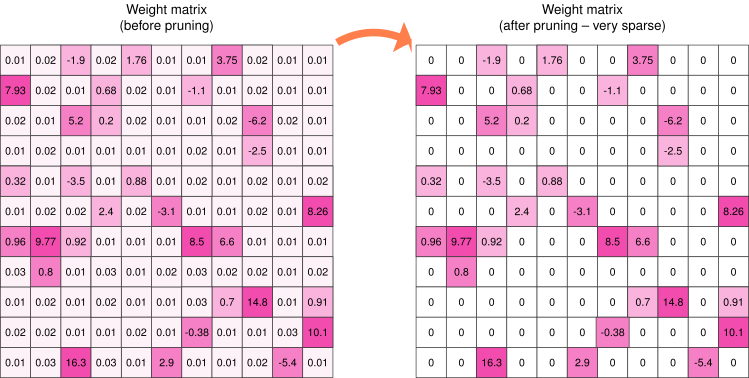](https://mlsysbook.ai/contents/core/optimizations/a89a4ba7c99fed29c85450f3d327e3056354e1f0.svg "Figure 2: Sparse Matrix Transformation: Pruning removes small-magnitude weights (shown as white/zero in the right matrix) while preserving large-magnitude weights (shown in color), creating a sparse representation that reduces both memory usage and computation while maintaining model accuracy.")
Figure 2: **Sparse Matrix Transformation**: Pruning removes small-magnitude weights (shown as white/zero in the right matrix) while preserving large-magnitude weights (shown in color), creating a sparse representation that reduces both memory usage and computation while maintaining model accuracy.
#### Mathematical Formulation
The goal of pruning can be stated simply: we want to find the version of our model that has the fewest non-zero weights (the smallest size) while causing the smallest possible increase in the prediction error (the loss). This intuitive goal translates into a mathematical optimization problem that guides practical pruning algorithms.
The pruning process can be formalized as an optimization problem. Given a trained model with parameters \\(W\\), we seek a sparse version \\(\\hat{W}\\) that retains only the most important parameters. The objective is expressed as:
\\\[ \\min\_{\\hat{W}} \\mathcal{L}(\\hat{W}) \\quad \\text{subject to} \\quad \\|\\hat{W}\\|\_0 \\leq k \\\]
where \\(\\mathcal{L}(\\hat{W})\\) represents the model’s loss function after pruning, \\(\\hat{W}\\) denotes the pruned model’s parameters, \\(\\|\\hat{W}\\|\_0\\) is the L0-norm (number of nonzero parameters), and \\(k\\) is the parameter budget constraining maximum model size.
The L0-norm directly measures model size by counting nonzero parameters, which determines memory usage and computational cost. However, L0-norm minimization is NP-hard, making this optimization challenging. Practical pruning algorithms use heuristics like magnitude-based selection, gradient-based importance, or second-order sensitivity to approximate solutions efficiently.
In [Listing 1](https://mlsysbook.ai/contents/core/optimizations/optimizations.html#lst-pruning_example)
, this constraint becomes concrete: we reduced \\(\\|\\hat{W}\\|\_0\\) from 9 to 4 (satisfying \\(k=4\\)), with the magnitude threshold acting as our selection heuristic. Alternative formulations using L1 or L2 norms encourage small weights but don’t guarantee exact zeros, failing to reduce actual memory or computation without explicit thresholding.
To make pruning computationally feasible, practical methods replace the hard constraint with a soft regularization term: \\\[ \\min\_W \\mathcal{L}(W) + \\lambda \\| W \\|\_1 \\\] where \\(\\lambda\\) controls sparsity degree. The \\(\\ell\_1\\)\-norm encourages smaller weight values and promotes sparsity but does not strictly enforce zero values. Other methods use iterative heuristics, where parameters with smallest magnitudes are pruned in successive steps, followed by fine-tuning to recover lost accuracy ([Gale, Elsen, and Hooker 2019a](https://mlsysbook.ai/contents/core/optimizations/optimizations.html#ref-gale2020sparse)
; [Labarge, n.d.](https://mlsysbook.ai/contents/core/optimizations/optimizations.html#ref-blalock2020state)
).
———. 2019a. “The State of Sparsity in Deep Neural Networks.” _arXiv Preprint arXiv:1902.09574_, February. [http://arxiv.org/abs/1902.09574v1](http://arxiv.org/abs/1902.09574v1)
.
#### Target Structures
Pruning methods vary based on which structures within a neural network are removed. The primary targets include neurons, channels, and layers, each with distinct implications for the model’s architecture and performance.
* **Neuron pruning** removes entire neurons along with their associated weights and biases, reducing the width of a layer. This technique is often applied to fully connected layers.
* **Channel pruning** (or filter pruning), commonly used in convolutional neural networks, eliminates entire channels or filters. This reduces the depth of feature maps, which impacts the network’s ability to extract certain features. Channel pruning is particularly valuable in image-processing tasks where computational efficiency is a priority.
* **Layer pruning** removes entire layers from the network, significantly reducing depth. While this approach can yield significant efficiency gains, it requires careful balance to ensure the model retains sufficient capacity to capture complex patterns.
[Figure 3](https://mlsysbook.ai/contents/core/optimizations/optimizations.html#fig-channel-layer-pruning)
illustrates the differences between channel pruning and layer pruning. When a channel is pruned, the model’s architecture must be adjusted to accommodate the structural change. Specifically, the number of input channels in subsequent layers must be modified, requiring alterations to the depths of the filters applied to the layer with the removed channel. In contrast, layer pruning removes all channels within a layer, necessitating more significant architectural modifications. In this case, connections between remaining layers must be reconfigured to bypass the removed layer. Regardless of the pruning approach, fine-tuning is important to adapt the remaining network and restore performance.
[](https://mlsysbook.ai/contents/core/optimizations/c119c964bcc3ea8df03d4b0eae20702de43d77d8.svg "Figure 3: Pruning Strategies: Channel pruning adjusts filter sizes within layers, while layer pruning removes entire layers and necessitates reconnection of remaining network components. These approaches reduce model size and computational cost, but require fine-tuning to mitigate performance loss due to reduced model capacity.")
Figure 3: **Pruning Strategies**: Channel pruning adjusts filter sizes within layers, while layer pruning removes entire layers and necessitates reconnection of remaining network components. These approaches reduce model size and computational cost, but require fine-tuning to mitigate performance loss due to reduced model capacity.
#### Unstructured Pruning
Unstructured pruning removes individual weights while preserving the overall network architecture. During training, some connections become redundant, contributing little to the final computation. Pruning these weak connections reduces memory requirements while preserving most of the model’s accuracy.
The mathematical foundation for unstructured pruning helps understand how sparsity is systematically introduced. Mathematically, unstructured pruning introduces sparsity into the weight matrices of a neural network. Let \\(W \\in \\mathbb{R}^{m \\times n}\\) represent a weight matrix in a given layer of a network. Pruning removes a subset of weights by applying a binary mask \\(M \\in \\{0,1\\}^{m \\times n}\\), yielding a pruned weight matrix: \\\[ \\hat{W} = M \\odot W \\\] where \\(\\odot\\) represents the element-wise Hadamard product. The mask \\(M\\) is constructed based on a pruning criterion, typically weight magnitude. A common approach is magnitude-based pruning, which removes a fraction \\(s\\) of the lowest-magnitude weights. This is achieved by defining a threshold \\(\\tau\\) such that: \\\[ M\_{i,j} = \\begin{cases} 1, & \\text{if } |W\_{i,j}| > \\tau \\\\ 0, & \\text{otherwise} \\end{cases} \\\] where \\(\\tau\\) is chosen to ensure that only the largest \\((1 - s)\\) fraction of weights remain. This method assumes that larger-magnitude weights contribute more to the network’s function, making them preferable for retention.
The primary advantage of unstructured pruning is memory efficiency. By reducing the number of nonzero parameters, pruned models require less storage, which is particularly beneficial when deploying models to embedded or mobile devices with limited memory.
However, unstructured pruning does not necessarily improve computational efficiency on modern machine learning hardware. Standard GPUs and TPUs are optimized for dense matrix multiplications, and a sparse weight matrix often cannot fully utilize hardware acceleration unless specialized sparse computation kernels are available. Therefore, unstructured pruning primarily benefits model storage rather than inference acceleration. While unstructured pruning improves model efficiency at the parameter level, it does not alter the structural organization of the network.
#### Structured Pruning
While unstructured pruning removes individual weights from a neural network, structured pruning[15](https://mlsysbook.ai/contents/core/optimizations/optimizations.html#fn15)
eliminates entire computational units, such as neurons, filters, channels, or layers. This approach is particularly beneficial for hardware efficiency, as it produces smaller dense models that can be directly mapped to modern machine learning accelerators. Unlike unstructured pruning, which results in sparse weight matrices that require specialized execution kernels to exploit computational benefits, structured pruning leads to more efficient inference on general-purpose hardware by reducing the overall size of the network architecture.
15 **Structured Pruning**: Filter pruning in ResNet-34 achieves 50% FLOP reduction with only 1.0% accuracy loss on CIFAR-10. Channel pruning in MobileNetV2 reduces parameters by 73% while maintaining 96.5% of original accuracy, enabling 3.2x faster inference on ARM processors.
Structured pruning is motivated by the observation that not all neurons, filters, or layers contribute equally to a model’s predictions. Some units primarily carry redundant or low-impact information, and removing them does not significantly degrade model performance. The challenge lies in identifying which structures can be pruned while preserving accuracy.
[Figure 4](https://mlsysbook.ai/contents/core/optimizations/optimizations.html#fig-structured-unstructured)
illustrates the key differences between unstructured and structured pruning. On the left, unstructured pruning removes individual weights (depicted as dashed connections), creating a sparse weight matrix. This can disrupt the original network structure, as shown in the fully connected network where certain connections have been randomly pruned. While this reduces the number of active parameters, the resulting sparsity requires specialized execution kernels to fully utilize computational benefits.
In contrast, structured pruning (depicted in the middle and right sections of the figure) removes entire neurons or filters while preserving the network’s overall structure. In the middle section, a pruned fully connected network retains its fully connected nature but with fewer neurons. On the right, structured pruning is applied to a CNN by removing convolutional kernels or entire channels (dashed squares). This method maintains the CNN’s core convolutional operations while reducing the computational load, making it more compatible with hardware accelerators.
[](https://mlsysbook.ai/contents/core/optimizations/03511cbb93a9ca744f76c0f625e9aee09f8a8f06.svg "Figure 4: Pruning Strategies: Unstructured pruning achieves sparsity by removing individual weights, requiring specialized hardware for efficient computation, while structured pruning removes entire neurons or filters, preserving network structure and enabling acceleration on standard hardware. This figure contrasts the resulting weight matrices and network architectures from both approaches, highlighting the trade-offs between sparsity level and computational efficiency. Source: [@qi2021efficient].")
Figure 4: **Pruning Strategies**: Unstructured pruning achieves sparsity by removing individual weights, requiring specialized hardware for efficient computation, while structured pruning removes entire neurons or filters, preserving network structure and enabling acceleration on standard hardware. This figure contrasts the resulting weight matrices and network architectures from both approaches, highlighting the trade-offs between sparsity level and computational efficiency. Source: ([Qi et al. 2021](https://mlsysbook.ai/contents/core/optimizations/optimizations.html#ref-qi2021efficient)
).
Qi, Chen, Shibo Shen, Rongpeng Li, Zhifeng Zhao, Qing Liu, Jing Liang, and Honggang Zhang. 2021. “An Efficient Pruning Scheme of Deep Neural Networks for Internet of Things Applications.” _EURASIP Journal on Advances in Signal Processing_ 2021 (1): 31. [https://doi.org/10.1186/s13634-021-00744-4](https://doi.org/10.1186/s13634-021-00744-4)
.
A common approach to structured pruning is magnitude-based pruning, where entire neurons or filters are removed based on the magnitude of their associated weights. The intuition behind this method is that parameters with smaller magnitudes contribute less to the model’s output, making them prime candidates for elimination. The importance of a neuron or filter is often measured using a norm function, such as the \\(\\ell\_1\\)\-norm or \\(\\ell\_2\\)\-norm, applied to the weights associated with that unit. If the norm falls below a predefined threshold, the corresponding neuron or filter is pruned. This method is straightforward to implement and does not require additional computational overhead beyond computing norms across layers.
Another strategy is activation-based pruning, which evaluates the average activation values of neurons or filters over a dataset. Neurons that consistently produce low activations contribute less information to the network’s decision process and can be safely removed. This method captures the dynamic behavior of the network rather than relying solely on static weight values. Activation-based pruning requires profiling the model over a representative dataset to estimate the average activation magnitudes before making pruning decisions.
Gradient-based pruning uses information from the model’s training process to identify less significant neurons or filters. The key idea is that units with smaller gradient magnitudes contribute less to reducing the loss function, making them less important for learning. By ranking neurons based on their gradient values, structured pruning can remove those with the least impact on model optimization. Unlike magnitude-based or activation-based pruning, which rely on static properties of the trained model, gradient-based pruning requires access to gradient computations and is typically applied during training rather than as a post-processing step.
Each of these methods presents trade-offs in terms of computational complexity and effectiveness. Magnitude-based pruning is computationally inexpensive and easy to implement but does not account for how neurons behave across different data distributions. Activation-based pruning provides a more data-driven pruning approach but requires additional computations to estimate neuron importance. Gradient-based pruning leverages training dynamics but may introduce additional complexity if applied to large-scale models. The choice of method depends on the specific constraints of the target deployment environment and the performance requirements of the pruned model.
#### Dynamic Pruning
Traditional pruning methods, whether unstructured or structured, typically involve static pruning, where parameters are permanently removed after training or at fixed intervals during training. However, this approach assumes that the importance of parameters is fixed, which is not always the case. In contrast, dynamic pruning adapts pruning decisions based on the input data or training dynamics, allowing the model to adjust its structure in real time.
Dynamic pruning can be implemented using runtime sparsity techniques, where the model actively determines which parameters to utilize based on input characteristics. Activation-conditioned pruning exemplifies this approach by selectively deactivating neurons or channels that exhibit low activation values for specific inputs ([J. Hu et al. 2023](https://mlsysbook.ai/contents/core/optimizations/optimizations.html#ref-dynamicpruning2023)
). This method introduces input-dependent sparsity patterns, effectively reducing the computational workload during inference without permanently modifying the model architecture.
Hu, Jie, Peng Lin, Huajun Zhang, Zining Lan, Wenxin Chen, Kailiang Xie, Siyun Chen, Hao Wang, and Sheng Chang. 2023. “A Dynamic Pruning Method on Multiple Sparse Structures in Deep Neural Networks.” _IEEE Access_ 11: 38448–57. [https://doi.org/10.1109/access.2023.3267469](https://doi.org/10.1109/access.2023.3267469)
.
For instance, consider a convolutional neural network processing images with varying complexity. During inference of a simple image containing mostly uniform regions, many convolutional filters may produce negligible activations. Dynamic pruning identifies these low-impact filters and temporarily excludes them from computation, improving efficiency while maintaining accuracy for the current input. This adaptive behavior is particularly advantageous in latency-sensitive applications, where computational resources must be allocated judiciously based on input complexity, connecting to performance measurement strategies (**[Chapter 12: Benchmarking AI](https://mlsysbook.ai/contents/core/benchmarking/benchmarking.html#sec-benchmarking-ai)
**).
Another class of dynamic pruning operates during training, where sparsity is gradually introduced and adjusted throughout the optimization process. Methods such as gradual magnitude pruning start with a dense network and progressively increase the fraction of pruned parameters as training progresses. Instead of permanently removing parameters, these approaches allow the network to recover from pruning-induced capacity loss by regrowing connections that prove to be important in later stages of training.
Dynamic pruning presents several advantages over static pruning. It allows models to adapt to different workloads, potentially improving efficiency while maintaining accuracy. Unlike static pruning, which risks over-pruning and degrading performance, dynamic pruning provides a mechanism for selectively reactivating parameters when necessary. However, implementing dynamic pruning requires additional computational overhead, as pruning decisions must be made in real-time, either during training or inference. This makes it more complex to integrate into standard machine learning pipelines compared to static pruning, requiring sophisticated production deployment strategies and monitoring frameworks covered in **[Chapter 13: ML Operations](https://mlsysbook.ai/contents/core/ops/ops.html#sec-ml-operations)
**.
Despite its challenges, dynamic pruning is particularly useful in edge computing and adaptive AI systems (**[Chapter 14: On-Device Learning](https://mlsysbook.ai/contents/core/ondevice_learning/ondevice_learning.html#sec-ondevice-learning)
**), where resource constraints and real-time efficiency requirements vary across different inputs. The next section explores the practical considerations and trade-offs involved in choosing the right pruning method for a given machine learning system.
#### Pruning Trade-offs
Pruning techniques offer different trade-offs in terms of memory efficiency, computational efficiency, accuracy retention, hardware compatibility, and implementation complexity. The choice of pruning strategy depends on the specific constraints of the machine learning system and the deployment environment, integrating with operational considerations (**[Chapter 13: ML Operations](https://mlsysbook.ai/contents/core/ops/ops.html#sec-ml-operations)
**).
Unstructured pruning is particularly effective in reducing model size and memory footprint, as it removes individual weights while keeping the overall model architecture intact. However, since machine learning accelerators are optimized for dense matrix operations, unstructured pruning does not always translate to significant computational speed-ups unless specialized sparse execution kernels are used.
Structured pruning, in contrast, eliminates entire neurons, channels, or layers, leading to a more hardware-friendly model. This technique provides direct computational savings, as it reduces the number of floating-point operations (FLOPs)[16](https://mlsysbook.ai/contents/core/optimizations/optimizations.html#fn16)
required during inference.
16 **FLOPs (Floating-Point Operations)**: Computational complexity metric counting multiply-add operations. ResNet-50 requires approximately 3.8 billion FLOPs per inference ([K. He et al. 2015](https://mlsysbook.ai/contents/core/optimizations/optimizations.html#ref-he2016deep)
), GPT-3 training required an estimated 3.14E23 FLOPs ([Patterson et al. 2021](https://mlsysbook.ai/contents/core/optimizations/optimizations.html#ref-patterson2021carbon)
). Modern GPUs achieve 100-300 TFLOPS (trillion FLOPs/second), making FLOP reduction important for efficiency.
He, Kaiming, Xiangyu Zhang, Shaoqing Ren, and Jian Sun. 2015. “Deep Residual Learning for Image Recognition,” December, 770–78. [https://doi.org/10.1109/CVPR.2016.90](https://doi.org/10.1109/CVPR.2016.90)
.
Patterson, David, Joseph Gonzalez, Quoc Le, Chen Liang, Lluis-Miquel Munguia, Daniel Rothchild, David So, Maud Texier, and Jeff Dean. 2021. “Carbon Emissions and Large Neural Network Training.” _arXiv Preprint arXiv:2104.10350_, April. [http://arxiv.org/abs/2104.10350v3](http://arxiv.org/abs/2104.10350v3)
.
The downside is that modifying the network structure can lead to a greater accuracy drop, requiring careful fine-tuning to recover lost performance.
Dynamic pruning introduces adaptability into the pruning process by adjusting which parameters are pruned at runtime based on input data or training dynamics. This allows for a better balance between accuracy and efficiency, as the model retains the flexibility to reintroduce previously pruned parameters if needed. However, dynamic pruning increases implementation complexity, as it requires additional computations to determine which parameters to prune on-the-fly.
[Table 2](https://mlsysbook.ai/contents/core/optimizations/optimizations.html#tbl-pruning)
summarizes the key structural differences between these pruning approaches, outlining how each method modifies the model and impacts its execution.
Table 2: **Pruning Strategies**: Unstructured, structured, and dynamic pruning each modify model weights differently, impacting both model size and computational efficiency; unstructured pruning offers the greatest compression but requires specialized hardware, while dynamic pruning adapts to input data for a balance between accuracy and resource usage.
| | | | |
| --- | --- | --- | --- |
| **What is removed?** | Individual weights in the model | Entire neurons, channels, filters, or layers | Adjusts pruning based on runtime conditions |
| **Model structure** | Sparse weight matrices; original architecture remains unchanged | Model architecture is modified; pruned layers are fully removed | Structure adapts dynamically |
| **Impact on memory** | Reduces model storage by eliminating nonzero weights | Reduces model storage by removing entire components | Varies based on real-time pruning |
| **Impact on computation** | Limited; dense matrix operations still required unless specialized sparse computation is used | Directly reduces FLOPs and speeds up inference | Balances accuracy and efficiency dynamically |
| **Hardware compatibility** | Sparse weight matrices require specialized execution support for efficiency | Works efficiently with standard deep learning hardware | Requires adaptive inference engines |
| **Fine-tuning required?** | Often necessary to recover accuracy after pruning | More likely to require fine-tuning due to larger structural modifications | Adjusts dynamically, reducing the need for retraining |
| **Use cases** | Memory-efficient model compression, particularly for cloud deployment | Real-time inference optimization, mobile/edge AI, and efficient training | Adaptive AI applications, real-time systems |
#### Pruning Strategies
Beyond the broad categories of unstructured, structured, and dynamic pruning, different pruning workflows can impact model efficiency and accuracy retention. Two widely used pruning strategies are iterative pruning and one-shot pruning, each with its own benefits and trade-offs.
##### Iterative Pruning
Iterative pruning implements a gradual approach to structure removal through multiple cycles of pruning followed by fine-tuning. During each cycle, the algorithm removes a small subset of structures based on predefined importance metrics. The model then undergoes fine-tuning to adapt to these structural modifications before proceeding to the next pruning iteration. This methodical approach helps prevent sudden drops in accuracy while allowing the network to progressively adjust to reduced complexity.
To illustrate this process, consider pruning six channels from a convolutional neural network as shown in [Figure 5](https://mlsysbook.ai/contents/core/optimizations/optimizations.html#fig-iterative-pruning)
. Rather than removing all channels simultaneously, iterative pruning eliminates two channels per iteration over three cycles. Following each pruning step, the model undergoes fine-tuning to recover performance. The first iteration, which removes two channels, results in an accuracy decrease from 0.995 to 0.971, but subsequent fine-tuning restores accuracy to 0.992. After completing two additional pruning-tuning cycles, the final model achieves 0.991 accuracy, which represents only a 0.4% reduction from the original, while operating with 27% fewer channels. By distributing structural modifications across multiple iterations, the network maintains its performance capabilities while achieving improved computational efficiency.
[](https://mlsysbook.ai/contents/core/optimizations/b4f4852e7bfe246bb537f3af5ec1e584289eac85.svg "Figure 5: Iterative Pruning Performance: Gradual channel removal with interleaved fine-tuning maintains high accuracy while reducing model size; this figure provides a 0.4% accuracy drop with a 27% reduction in channels, showcasing the benefits of distributing structural modifications across multiple iterations. This approach contrasts with one-shot pruning, which often leads to significant performance degradation.")
Figure 5: **Iterative Pruning Performance**: Gradual channel removal with interleaved fine-tuning maintains high accuracy while reducing model size; this figure provides a 0.4% accuracy drop with a 27% reduction in channels, showcasing the benefits of distributing structural modifications across multiple iterations. This approach contrasts with one-shot pruning, which often leads to significant performance degradation.
##### One-shot Pruning
One-shot pruning removes multiple architectural components in a single step, followed by an extensive fine-tuning phase to recover model accuracy. This aggressive approach compresses the model quickly but risks greater accuracy degradation, as the network must adapt to significant structural changes simultaneously.
Consider applying one-shot pruning to the same network from the iterative pruning example. Instead of removing two channels at a time over multiple iterations, one-shot pruning eliminates all six channels simultaneously, as illustrated in [Figure 6](https://mlsysbook.ai/contents/core/optimizations/optimizations.html#fig-oneshot-pruning)
. Removing 27% of the network’s channels simultaneously causes the accuracy to drop significantly, from 0.995 to 0.914. Even after fine-tuning, the network only recovers to an accuracy of 0.943, which is a 5% degradation from the original unpruned network. While both iterative and one-shot pruning ultimately produce identical network structures, the gradual approach of iterative pruning better preserves model performance.
[](https://mlsysbook.ai/contents/core/optimizations/0a60b8e71484b67b7d2e37ef7bdc4e8f900c7ba1.svg "Figure 6: One-Shot Pruning Impact: Aggressive removal of architectural components, like the 27% of channels shown, causes significant initial accuracy loss because the network struggles to adapt to significant structural changes simultaneously. Fine-tuning partially recovers performance, but establishes that iterative pruning preserves accuracy more effectively than single-step approaches.")
Figure 6: **One-Shot Pruning Impact**: Aggressive removal of architectural components, like the 27% of channels shown, causes significant initial accuracy loss because the network struggles to adapt to significant structural changes simultaneously. Fine-tuning partially recovers performance, but establishes that iterative pruning preserves accuracy more effectively than single-step approaches.
The choice of pruning strategy requires careful consideration of several key factors that influence both model efficiency and performance. The desired level of parameter reduction, or sparsity target, directly impacts strategy selection. Higher reduction targets often necessitate iterative approaches to maintain accuracy, while moderate sparsity goals may be achievable through simpler one-shot methods.
Available computational resources significantly influence strategy choice. Iterative pruning demands significant resources for multiple fine-tuning cycles, whereas one-shot approaches require fewer resources but may sacrifice accuracy. This resource consideration connects to performance requirements, where applications with strict accuracy requirements typically benefit from gradual, iterative pruning to carefully preserve model capabilities. Use cases with more flexible performance constraints may accommodate more aggressive one-shot approaches.
Development timeline also impacts pruning decisions. One-shot methods enable faster deployment when time is limited, though iterative approaches generally achieve superior results given sufficient optimization periods. Finally, target platform capabilities significantly influence strategy selection, as certain hardware architectures may better support specific sparsity patterns, making particular pruning approaches more advantageous for deployment.
The choice between pruning strategies requires careful evaluation of project requirements and constraints. One-shot pruning enables rapid model compression by removing multiple parameters simultaneously, making it suitable for scenarios where deployment speed is prioritized over accuracy. However, this aggressive approach often results in greater performance degradation compared to more gradual methods. Iterative pruning, on the other hand, while computationally intensive and time-consuming, typically achieves superior accuracy retention through structured parameter reduction across multiple cycles. This methodical approach enables the network to adapt progressively to structural modifications, preserving important connections that maintain model performance. The trade-off is increased optimization time and computational overhead. By evaluating these factors systematically, practitioners can select a pruning approach that optimally balances efficiency gains with model performance for their specific use case.
#### Lottery Ticket Hypothesis
Pruning is widely used to reduce the size and computational cost of neural networks, but the process of determining which parameters to remove is not always straightforward. While traditional pruning methods eliminate weights based on magnitude, structure, or dynamic conditions, recent research suggests that pruning is not just about reducing redundancy; it may also reveal inherently efficient subnetworks that exist within the original model.
This perspective leads to the Lottery Ticket Hypothesis[17](https://mlsysbook.ai/contents/core/optimizations/optimizations.html#fn17)
(LTH), which challenges conventional pruning workflows by proposing that within large neural networks, there exist small, well-initialized subnetworks, referred to as ‘winning tickets’, that can achieve comparable accuracy to the full model when trained in isolation. Rather than viewing pruning as just a post-training compression step, LTH suggests it can serve as a discovery mechanism to identify these efficient subnetworks early in training.
17 **Lottery Ticket Hypothesis**: The lottery ticket hypothesis ([Frankle and Carbin 2018](https://mlsysbook.ai/contents/core/optimizations/optimizations.html#ref-frankle2018lottery)
) demonstrates that ResNet-18 subnetworks at 10-20% original size achieve 93.2% accuracy vs. 94.1% for full model on CIFAR-10. BERT-base winning tickets retain 97% performance with 90% fewer parameters, requiring 5-8x less training time to converge.
Frankle, Jonathan, and Michael Carbin. 2018. “The Lottery Ticket Hypothesis: Finding Sparse, Trainable Neural Networks.” _arXiv Preprint arXiv:1803.03635_, March. [http://arxiv.org/abs/1803.03635v5](http://arxiv.org/abs/1803.03635v5)
.
LTH is validated through an iterative pruning process, illustrated in [Figure 7](https://mlsysbook.ai/contents/core/optimizations/optimizations.html#fig-winning-ticket)
. A large network is first trained to convergence. The lowest-magnitude weights are then pruned, and the remaining weights are reset to their original initialization rather than being re-randomized. This process is repeated iteratively, gradually reducing the network’s size while preserving performance. After multiple iterations, the remaining subnetwork, referred to as the ‘winning ticket’, proves capable of training to the same or higher accuracy as the original full model.
[](https://mlsysbook.ai/contents/core/optimizations/29c8368c161464faafe599cd9811aa1fee3484fc.svg "Figure 7: Winning Ticket Discovery: Iterative pruning and weight resetting identify subnetworks within larger models that, when trained in isolation, achieve comparable or superior accuracy, challenging the conventional view of pruning as solely a compression technique. This process establishes that well-initialized subnetworks exist and can be efficiently trained, suggesting that much of a large network’s capacity may be redundant.")
Figure 7: **Winning Ticket Discovery**: Iterative pruning and weight resetting identify subnetworks within larger models that, when trained in isolation, achieve comparable or superior accuracy, challenging the conventional view of pruning as solely a compression technique. This process establishes that well-initialized subnetworks exist and can be efficiently trained, suggesting that much of a large network’s capacity may be redundant.
The implications of the Lottery Ticket Hypothesis extend beyond conventional pruning techniques. Instead of training large models and pruning them later, LTH suggests that compact, high-performing subnetworks could be trained directly from the start, eliminating the need for overparameterization. This insight challenges the traditional assumption that model size is necessary for effective learning. It also emphasizes the importance of initialization, as winning tickets only retain their performance when reset to their original weight values. This finding raises deeper questions about the role of initialization in shaping a network’s learning trajectory.
The hypothesis further reinforces the effectiveness of iterative pruning over one-shot pruning. Gradually refining the model structure allows the network to adapt at each stage, preserving accuracy more effectively than removing large portions of the model in a single step. This process aligns well with practical pruning strategies used in deployment, where preserving accuracy while reducing computation is important.
Despite its promise, applying LTH in practice remains computationally expensive, as identifying winning tickets requires multiple cycles of pruning and retraining. Ongoing research explores whether winning subnetworks can be detected early without full training, potentially leading to more efficient sparse training techniques. If such methods become practical, LTH could corely reshape how machine learning models are trained, shifting the focus from pruning large networks after training to discovering and training only the important components from the beginning.
While LTH presents a compelling theoretical perspective on pruning, practical implementations rely on established framework-level tools to integrate structured and unstructured pruning techniques.
#### Pruning Practice
Several machine learning frameworks provide built-in tools to apply structured and unstructured pruning, fine-tune pruned models, and optimize deployment for cloud, edge, and mobile environments.
Machine learning frameworks such as PyTorch, TensorFlow, and ONNX offer dedicated pruning utilities that allow practitioners to efficiently implement these techniques while ensuring compatibility with deployment hardware.
In PyTorch, pruning is available through the `torch.nn.utils.prune` module, which provides functions to apply magnitude-based pruning to individual layers or the entire model. Users can perform unstructured pruning by setting a fraction of the smallest-magnitude weights to zero or apply structured pruning to remove entire neurons or filters. PyTorch also allows for custom pruning strategies, where users define pruning criteria beyond weight magnitude, such as activation-based or gradient-based pruning. Once a model is pruned, it can be fine-tuned to recover lost accuracy before being exported for inference.
TensorFlow provides pruning support through the TensorFlow Model Optimization Toolkit (TF-MOT). This toolkit integrates pruning directly into the training process by applying sparsity-inducing regularization. TensorFlow’s pruning API supports global and layer-wise pruning, dynamically selecting parameters for removal based on weight magnitudes. Unlike PyTorch, TensorFlow’s pruning is typically applied during training, allowing models to learn sparse representations from the start rather than pruning them post-training. TF-MOT also provides export tools to convert pruned models into TFLite format, making them compatible with mobile and edge devices.
ONNX[18](https://mlsysbook.ai/contents/core/optimizations/optimizations.html#fn18)
, an open standard for model representation, does not implement pruning directly but provides export and compatibility support for pruned models from PyTorch and TensorFlow. Since ONNX is designed to be hardware-agnostic, it allows models that have undergone pruning in different frameworks to be optimized for inference engines such as TensorRT[19](https://mlsysbook.ai/contents/core/optimizations/optimizations.html#fn19)
, OpenVINO, and EdgeTPU. These inference engines can further leverage structured and dynamic pruning for execution efficiency, particularly on specialized hardware accelerators.
18 **ONNX Deployment**: ONNX Runtime achieves 1.3-2.9x speedup over TensorFlow and 1.1-1.7x over PyTorch across various models on CPU platforms. ResNet-50 inference drops from 7.2ms to 2.8ms on CPU, while BERT-Base reduces from 45ms to 23ms with ONNX Runtime optimizations including graph fusion and memory pooling.
19 **TensorRT Optimization**: NVIDIA TensorRT delivers up to 40x speedup for inference compared to CPU baselines, with typical GPU optimization improvements of 5-8x on V100. ResNet-50 INT8 inference achieves 1.2ms vs. 4.8ms FP32, while BERT-Large drops from 10.4ms to 2.1ms. Layer fusion reduces kernel launches by 80%, memory bandwidth by 50%.
Although framework-level support for pruning has advanced significantly, applying pruning in practice requires careful consideration of hardware compatibility and software optimizations. Standard CPUs and GPUs often do not natively accelerate sparse matrix operations, meaning that unstructured pruning may reduce memory usage without providing significant computational speed-ups. In contrast, structured pruning is more widely supported in inference engines, as it directly reduces the number of computations needed during execution. Dynamic pruning, when properly integrated with inference engines, can optimize execution based on workload variations and hardware constraints, making it particularly beneficial for adaptive AI applications.
At a practical level, choosing the right pruning strategy depends on several key trade-offs, including memory efficiency, computational performance, accuracy retention, and implementation complexity. These trade-offs impact how pruning methods are applied in real-world machine learning workflows, influencing deployment choices based on resource constraints and system requirements.
To help guide these decisions, [Table 3](https://mlsysbook.ai/contents/core/optimizations/optimizations.html#tbl-pruning-tradeoffs)
provides a high-level comparison of these trade-offs, summarizing the key efficiency and usability factors that practitioners must consider when selecting a pruning method.
These trade-offs underscore the importance of aligning pruning methods with practical deployment needs. Frameworks such as PyTorch, TensorFlow, and ONNX enable developers to implement these strategies, but the effectiveness of a pruning approach depends on the underlying hardware and application requirements.
Table 3: **Pruning Trade-Offs**: Different pruning strategies balance memory efficiency, computational speed, accuracy retention, and hardware compatibility, impacting practical model deployment choices and system performance. Unstructured pruning offers high memory savings but requires specialized hardware, while structured pruning prioritizes computational efficiency at the cost of reduced accuracy.
| | | | |
| --- | --- | --- | --- |
| **Memory Efficiency** | ↑↑ High | ↑ Moderate | ↑ Moderate |
| **Computational Efficiency** | → Neutral | ↑↑ High | ↑ High |
| **Accuracy Retention** | ↑ Moderate | ↓↓ Low | ↑↑ High |
| **Hardware Compatibility** | ↓ Low | ↑↑ High | → Neutral |
| **Implementation Complexity** | → Neutral | ↑ Moderate | ↓↓ High |
For example, structured pruning is commonly used in mobile and edge applications because of its compatibility with standard inference engines, whereas dynamic pruning is better suited for adaptive AI workloads that need to adjust sparsity levels on the fly. Unstructured pruning, while useful for reducing memory footprints, requires specialized sparse execution kernels to fully realize computational savings.
Understanding these trade-offs is important when deploying pruned models in real-world settings. Several high-profile models have successfully integrated pruning to optimize performance. MobileNet, a lightweight convolutional neural network designed for mobile and embedded applications, has been pruned to reduce inference latency while preserving accuracy ([Howard et al. 2017](https://mlsysbook.ai/contents/core/optimizations/optimizations.html#ref-howard2017mobilenets)
). BERT[20](https://mlsysbook.ai/contents/core/optimizations/optimizations.html#fn20)
, a widely used transformer model for natural language processing, has undergone structured pruning of attention heads and intermediate layers to create efficient versions such as DistilBERT[21](https://mlsysbook.ai/contents/core/optimizations/optimizations.html#fn21)
and TinyBERT, which retain much of the original performance while reducing computational overhead ([Sanh et al. 2019](https://mlsysbook.ai/contents/core/optimizations/optimizations.html#ref-sanh2019distilbert)
). In computer vision, EfficientNet[22](https://mlsysbook.ai/contents/core/optimizations/optimizations.html#fn22)
has been pruned to remove unnecessary filters, optimizing it for deployment in resource-constrained environments ([Tan and Le 2019a](https://mlsysbook.ai/contents/core/optimizations/optimizations.html#ref-tan2019efficientnet)
).
20 **BERT Compression**: BERT-Base (110M params) can be compressed to 67M params (39% reduction) with only 1.2% GLUE score drop. Attention head pruning removes 144 of 192 heads with minimal impact, while layer pruning reduces 12 layers to 6 layers maintaining 97.8% performance.
21 **DistilBERT**: Achieves 97% of BERT-Base performance with 40% fewer parameters (66M vs. 110M) and 60% faster inference. On SQuAD v1.1, DistilBERT scores 86.9 F1 vs. BERT’s 88.5 F1, while reducing memory from 1.35GB to 0.54GB and latency from 85ms to 34ms.
22 **EfficientNet Pruning**: EfficientNet-B0 with 70% structured pruning maintains 75.8% ImageNet accuracy (vs. 77.1% original) with 2.8x speedup on mobile devices. Channel pruning reduces FLOPs from 390M to 140M while keeping inference under 20ms on Pixel 4.
Tan, Mingxing, and Quoc V Le. 2019a. “EfficientNet: Rethinking Model Scaling for Convolutional Neural Networks.” In _International Conference on Machine Learning (ICML)_, 6105–14.
### Knowledge Distillation
Imagine a world-class professor (the teacher model) who has read thousands of books and has a deep, nuanced understanding of a subject. Now, imagine a bright student (the student model) who needs to learn the subject quickly. Instead of just giving the student the textbook answers (the hard labels), the professor provides rich explanations, pointing out why one answer is better than another and how different concepts relate (the soft labels). The student learns much more effectively from this rich guidance than from the textbook alone. This is the essence of knowledge distillation.
Knowledge distillation trains a smaller student model using guidance from a larger pre-trained teacher, learning from the teacher’s rich output distributions rather than simple correct/incorrect labels. This distinction matters because teacher models provide richer learning signals than ground-truth labels. Consider image classification: a ground-truth label might say “this is a dog” (one-hot encoding: \[0, 1, 0, 0, …\]). But a trained teacher model might output \[0.02, 0.85, 0.08, 0.05, …\], revealing that while “dog” is most likely, the image shares some features with “wolf” (0.08) and “fox” (0.05). This inter-class similarity information helps the student learn feature relationships that hard labels cannot convey.
Knowledge distillation differs from pruning. While pruning removes parameters from an existing model, distillation trains a separate, smaller architecture using guidance from a larger pre-trained teacher ([Gou et al. 2021](https://mlsysbook.ai/contents/core/optimizations/optimizations.html#ref-gou2021knowledge)
). The student model optimizes to match the teacher’s soft predictions (probability distributions over classes) rather than simply learning from labeled data ([Jiong Lin et al. 2020](https://mlsysbook.ai/contents/core/optimizations/optimizations.html#ref-tang2020understanding)
).
Lin, Jiong, Qing Gao, Yungui Gong, Yizhou Lu, Chao Zhang, and Fengge Zhang. 2020. “Primordial Black Holes and Secondary Gravitational Waves from k/g Inflation.” _arXiv Preprint arXiv:2001.05909_, January. [http://arxiv.org/abs/2001.05909v2](http://arxiv.org/abs/2001.05909v2)
.
[Figure 8](https://mlsysbook.ai/contents/core/optimizations/optimizations.html#fig-kd-overview)
illustrates the distillation process. The teacher model produces probability distributions using a softened softmax function with temperature \\(T\\), and the student model trains using both these soft targets and ground truth labels.
[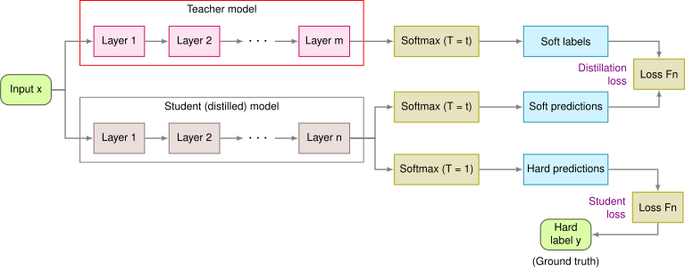](https://mlsysbook.ai/contents/core/optimizations/c4367bac55316f316802a7a1637be0c499035346.svg "Figure 8: Knowledge Distillation: A student model learns from the softened probability distributions generated by a pre-trained teacher model, transferring knowledge beyond hard labels. This process enables the student to achieve comparable performance to the teacher with fewer parameters by using the teacher’s generalization capabilities and inter-class relationships.")
Figure 8: **Knowledge Distillation**: A student model learns from the softened probability distributions generated by a pre-trained teacher model, transferring knowledge beyond hard labels. This process enables the student to achieve comparable performance to the teacher with fewer parameters by using the teacher’s generalization capabilities and inter-class relationships.
The training process for the student model incorporates two loss terms:
* **Distillation loss**: A loss function (often based on Kullback-Leibler (KL) divergence[23](https://mlsysbook.ai/contents/core/optimizations/optimizations.html#fn23)
) that minimizes the difference between the student’s and teacher’s soft label distributions.
* **Student loss**: A standard cross-entropy loss that ensures the student model correctly classifies the hard labels.
23 **Kullback-Leibler (KL) Divergence**: Information-theoretic measure quantifying difference between probability distributions, introduced by Kullback & Leibler ([Kullback and Leibler 1951](https://mlsysbook.ai/contents/core/optimizations/optimizations.html#ref-kullback1951information)
). In knowledge distillation, typical KL divergence values range 0.1-2.0 nats; values >3.0 indicate poor teacher-student alignment requiring temperature adjustment or architecture modification.
Kullback, S., and R. A. Leibler. 1951. “On Information and Sufficiency.” _The Annals of Mathematical Statistics_ 22 (1): 79–86. [https://doi.org/10.1214/aoms/1177729694](https://doi.org/10.1214/aoms/1177729694)
.
The combination of these two loss functions enables the student model to absorb both structured knowledge from the teacher and label supervision from the dataset. This approach allows smaller models to reach accuracy levels close to their larger teacher models, making knowledge distillation a key technique for model compression and efficient deployment.
Knowledge distillation allows smaller models to reach a level of accuracy that would be difficult to achieve through standard training alone. This makes it particularly useful in ML systems where inference efficiency is a priority, such as real-time applications, cloud-to-edge model compression, and low-power AI systems ([Sun et al. 2019](https://mlsysbook.ai/contents/core/optimizations/optimizations.html#ref-sun2019patient)
).
Sun, Siqi, Yu Cheng, Zhe Gan, and Jingjing Liu. 2019. “Patient Knowledge Distillation for BERT Model Compression.” In _Proceedings of the 2019 Conference on Empirical Methods in Natural Language Processing and the 9th International Joint Conference on Natural Language Processing (EMNLP-IJCNLP)_. Association for Computational Linguistics. [https://doi.org/10.18653/v1/d19-1441](https://doi.org/10.18653/v1/d19-1441)
.
#### Distillation Theory
Knowledge distillation is based on the idea that a well-trained teacher model encodes more information about the data distribution than just the correct class labels. In conventional supervised learning, a model is trained to minimize the cross-entropy loss[24](https://mlsysbook.ai/contents/core/optimizations/optimizations.html#fn24)
between its predictions and the ground truth labels. However, this approach only provides a hard decision boundary for each class, discarding potentially useful information about how the model relates different classes to one another ([Hinton, Vinyals, and Dean 2015](https://mlsysbook.ai/contents/core/optimizations/optimizations.html#ref-hinton2015distilling)
).
24 **Cross-Entropy Loss**: Standard loss function for classification tasks measuring difference between predicted and true probability distributions. For binary classification, ranges 0-∞ (lower is better); values >2.3 indicate poor performance (worse than random guessing). Computed as -log(predicted probability for true class).
Hinton, Geoffrey, Oriol Vinyals, and Jeff Dean. 2015. “Distilling the Knowledge in a Neural Network,” March. [https://doi.org/10.1002/0471743984.vse0673](https://doi.org/10.1002/0471743984.vse0673)
.
Gou, Jianping, Baosheng Yu, Stephen J. Maybank, and Dacheng Tao. 2021. “Knowledge Distillation: A Survey.” _International Journal of Computer Vision_ 129 (6): 1789–819. [https://doi.org/10.1007/s11263-021-01453-z](https://doi.org/10.1007/s11263-021-01453-z)
.
Knowledge distillation addresses this limitation by transferring additional information through the soft probability distributions produced by the teacher model. Instead of training the student model to match only the correct label, it is trained to match the teacher’s full probability distribution over all possible classes. This is achieved by introducing a temperature-scaled softmax function, which smooths the probability distribution, making it easier for the student model to learn from the teacher’s outputs ([Gou et al. 2021](https://mlsysbook.ai/contents/core/optimizations/optimizations.html#ref-gou2021knowledge)
).
#### Distillation Mathematics
To formalize this temperature-based approach, let \\(z\_i\\) be the logits (pre-softmax outputs) of the model for class \\(i\\). The standard softmax function computes class probabilities as: \\\[ p\_i = \\frac{\\exp(z\_i)}{\\sum\_j \\exp(z\_j)} \\\] where higher logits correspond to higher confidence in a class prediction.
In knowledge distillation, we introduce a temperature parameter[25](https://mlsysbook.ai/contents/core/optimizations/optimizations.html#fn25)
\\(T\\) that scales the logits before applying softmax: \\\[ p\_i(T) = \\frac{\\exp(z\_i / T)}{\\sum\_j \\exp(z\_j / T)} \\\] where a higher temperature produces a softer probability distribution, revealing more information about how the model distributes uncertainty across different classes.
25 **Temperature Parameter**: Controls softness of probability distributions in knowledge distillation. T=1 gives standard softmax, T=3-5 typical for distillation (revealing inter-class relationships), T=20+ creates nearly uniform distributions. Optimal temperatures: T=3 for CIFAR-10, T=4 for ImageNet, T=6 for language models like BERT.
The student model is then trained using a loss function that minimizes the difference between its output distribution and the teacher’s softened output distribution. The most common formulation combines two loss terms: \\\[ \\mathcal{L}\_{\\text{distill}} = (1 - \\alpha) \\mathcal{L}\_{\\text{CE}}(y\_s, y) + \\alpha T^2 \\sum\_i p\_i^T \\log p\_{i, s}^T \\\] where:
* \\(\\mathcal{L}\_{\\text{CE}}(y\_s, y)\\) is the standard cross-entropy loss between the student’s predictions \\(y\_s\\) and the ground truth labels \\(y\\).
* The second term minimizes the Kullback-Leibler (KL) divergence between the teacher’s softened predictions \\(p\_i^T\\) and the student’s predictions \\(p\_{i, s}^T\\).
* The factor \\(T^2\\) ensures that gradients remain appropriately scaled when using high-temperature values.
* The hyperparameter \\(\\alpha\\) balances the importance of the standard training loss versus the distillation loss.
By learning from both hard labels and soft teacher outputs, the student model benefits from the generalization power of the teacher, improving its ability to distinguish between similar classes even with fewer parameters.
#### Distillation Intuition
By learning from both hard labels and soft teacher outputs, the student model benefits from the generalization power of the teacher, improving its ability to distinguish between similar classes even with fewer parameters. Unlike conventional training, where a model learns only from binary correctness signals, knowledge distillation allows the student to absorb a richer understanding of the data distribution from the teacher’s predictions.
A key advantage of soft targets is that they provide relative confidence levels rather than just a single correct answer. Consider an image classification task where the goal is to distinguish between different animal species. A standard model trained with hard labels will only receive feedback on whether its prediction is right or wrong. If an image contains a cat, the correct label is “cat,” and all other categories, such as “dog” and “fox,” are treated as equally incorrect. However, a well-trained teacher model naturally understands that a cat is more visually similar to a dog than to a fox, and its soft output probabilities might look like [Figure 9](https://mlsysbook.ai/contents/core/optimizations/optimizations.html#fig-targets)
, where the relative confidence levels indicate that while “cat” is the most likely category, “dog” is still a plausible alternative, whereas “fox” is much less likely.
[](https://mlsysbook.ai/contents/core/optimizations/656290b9f3c16c4655946cc22beb8eda047bdaa7.svg "Figure 9: Soft Target Distribution: Relative confidence levels indicate which classes are more likely for a given input, showing that a model can express uncertainty and provide nuanced outputs beyond simple correct or incorrect labels.")
Figure 9: **Soft Target Distribution**: Relative confidence levels indicate which classes are more likely for a given input, showing that a model can express uncertainty and provide nuanced outputs beyond simple correct or incorrect labels.
Rather than simply forcing the student model to classify the image strictly as a cat, the teacher model provides a more nuanced learning signal, indicating that while “dog” is incorrect, it is a more reasonable mistake than “fox.” This subtle information helps the student model build better decision boundaries between similar classes, making it more robust to ambiguity in real-world data.
This effect is particularly useful in cases where training data is limited or noisy. A large teacher model trained on extensive data has already learned to generalize well, capturing patterns that might be difficult to discover with smaller datasets. The student benefits by inheriting this structured knowledge, acting as if it had access to a larger training signal than what is explicitly available.
Another key benefit of knowledge distillation is its regularization effect. Because soft targets distribute probability mass across multiple classes, they prevent the student model from overfitting to specific hard labels. This regularization improves model generalization and reduces sensitivity to adversarial inputs. Instead of confidently assigning a probability of 1.0 to the correct class and 0.0 to all others, the student learns to make more calibrated predictions, which improves its generalization performance. This is especially important when the student model has fewer parameters, as smaller networks are more prone to overfitting.
Finally, distillation helps compress large models into smaller, more efficient versions without major performance loss. This compression capability directly enables the sustainable AI practices **[Chapter 18: Sustainable AI](https://mlsysbook.ai/contents/core/sustainable_ai/sustainable_ai.html#sec-sustainable-ai)
** by reducing the environmental impact of model deployment while maintaining performance standards. Training a small model from scratch often results in lower accuracy because the model lacks the capacity to learn the complex representations that a larger network can capture. However, by using the knowledge of a well-trained teacher, the student can reach a higher accuracy than it would have on its own, making it a more practical choice for real-world ML deployments, particularly in edge computing, mobile applications, and other resource-constrained environments explored in **[Chapter 14: On-Device Learning](https://mlsysbook.ai/contents/core/ondevice_learning/ondevice_learning.html#sec-ondevice-learning)
**.
#### Efficiency Gains
Knowledge distillation’s efficiency benefits span three key areas: memory efficiency, computational efficiency, and deployment flexibility. Unlike pruning which modifies trained models, distillation trains compact models from the start using teacher guidance, enabling accuracy levels difficult to achieve through standard training alone ([Sanh et al. 2019](https://mlsysbook.ai/contents/core/optimizations/optimizations.html#ref-sanh2019distilbert)
), supporting structured evaluation approaches in **[Chapter 12: Benchmarking AI](https://mlsysbook.ai/contents/core/benchmarking/benchmarking.html#sec-benchmarking-ai)
**.
##### Memory and Model Compression
A key advantage of knowledge distillation is that it enables smaller models to retain much of the predictive power of larger models, significantly reducing memory footprint. This is particularly useful in resource-constrained environments such as mobile and embedded AI systems, where model size directly impacts storage requirements and load times.
For instance, models such as DistilBERT ([Sanh et al. 2019](https://mlsysbook.ai/contents/core/optimizations/optimizations.html#ref-sanh2019distilbert)
) in NLP and MobileNet distillation variants ([Howard et al. 2017](https://mlsysbook.ai/contents/core/optimizations/optimizations.html#ref-howard2017mobilenets)
) in computer vision have been shown to retain up to 97% of the accuracy of their larger teacher models while using only half the number of parameters. This level of compression is often superior to pruning, where aggressive parameter reduction can lead to deterioration in representational power.
Howard, Andrew G., Menglong Zhu, Bo Chen, Dmitry Kalenichenko, Weijun Wang, Tobias Weyand, Marco Andreetto, and Hartwig Adam. 2017. “MobileNets: Efficient Convolutional Neural Networks for Mobile Vision Applications.” _ArXiv Preprint_ abs/1704.04861 (April). [http://arxiv.org/abs/1704.04861v1](http://arxiv.org/abs/1704.04861v1)
.
Another key benefit of knowledge distillation is its ability to transfer robustness and generalization from the teacher to the student. Large models are often trained with extensive datasets and develop strong generalization capabilities, meaning they are less sensitive to noise and data shifts. A well-trained student model inherits these properties, making it less prone to overfitting and more stable across diverse deployment conditions. This is particularly useful in low-data regimes, where training a small model from scratch may result in poor generalization due to insufficient training examples.
##### Computation and Inference Speed
By training the student model to approximate the teacher’s knowledge in a more compact representation, distillation results in models that require fewer FLOPs per inference, leading to faster execution times. Unlike unstructured pruning, which may require specialized hardware support for sparse computation, a distilled model remains densely structured, making it more compatible with existing machine learning accelerators such as GPUs, TPUs, and edge AI chips ([Jiao et al. 2020](https://mlsysbook.ai/contents/core/optimizations/optimizations.html#ref-jiao2020tinybert)
).
Jiao, Xiaoqi, Yichun Yin, Lifeng Shang, Xin Jiang, Xiao Chen, Linlin Li, Fang Wang, and Qun Liu. 2020. “TinyBERT: Distilling BERT for Natural Language Understanding.” In _Findings of the Association for Computational Linguistics: EMNLP 2020_. Association for Computational Linguistics. [https://doi.org/10.18653/v1/2020.findings-emnlp.372](https://doi.org/10.18653/v1/2020.findings-emnlp.372)
.
In real-world deployments, this translates to:
* Reduced inference latency, which is important for real-time AI applications such as speech recognition, recommendation systems, and self-driving perception models.
* Lower energy consumption, making distillation particularly relevant for low-power AI on mobile devices and IoT systems.
* Higher throughput in cloud inference, where serving a distilled model allows large-scale AI applications to reduce computational cost while maintaining model quality.
For example, when deploying transformer models for NLP, organizations often use teacher-student distillation to create models that achieve similar accuracy at 2-4\\(\\times\\) lower latency, making it feasible to serve billions of requests per day with significantly lower computational overhead.
##### Deployment and System Considerations
Knowledge distillation is also effective in multi-task learning scenarios, where a single teacher model can guide multiple student models for different tasks. For example, in multi-lingual NLP models, a large teacher trained on multiple languages can transfer language-specific knowledge to smaller, task-specific student models, enabling efficient deployment across different languages without retraining from scratch. Similarly, in computer vision, a teacher trained on diverse object categories can distill knowledge into specialized students optimized for tasks such as face recognition, medical imaging, or autonomous driving.
Once a student model is distilled, it can be further optimized for hardware-specific acceleration using techniques such as pruning, quantization, and graph optimization. This ensures that compressed models remain inference-efficient across multiple hardware environments, particularly in edge AI and mobile deployments ([Gordon, Duh, and Andrews 2020](https://mlsysbook.ai/contents/core/optimizations/optimizations.html#ref-gordon2020compressing)
).
Gordon, Mitchell, Kevin Duh, and Nicholas Andrews. 2020. “Compressing BERT: Studying the Effects of Weight Pruning on Transfer Learning.” In _Proceedings of the 5th Workshop on Representation Learning for NLP_. Association for Computational Linguistics. [https://doi.org/10.18653/v1/2020.repl4nlp-1.18](https://doi.org/10.18653/v1/2020.repl4nlp-1.18)
.
Despite its advantages, knowledge distillation has some limitations. The effectiveness of distillation depends on the quality of the teacher model, a poorly trained teacher may transfer incorrect biases to the student. Distillation introduces an additional training phase, where both the teacher and student must be used together, increasing computational costs during training. In some cases, designing an appropriate student model architecture that can fully benefit from the teacher’s knowledge remains a challenge, as overly small student models may not have enough capacity to absorb all the relevant information.
#### Trade-offs
Compared to pruning, knowledge distillation preserves accuracy better but requires higher training complexity through training a new model rather than modifying an existing one. However, pruning provides a more direct computational efficiency gain, especially when structured pruning is used. In practice, combining pruning and distillation often yields the best trade-off, as seen in models like DistilBERT and MobileBERT, where pruning first reduces unnecessary parameters before distillation optimizes a final student model. [Table 4](https://mlsysbook.ai/contents/core/optimizations/optimizations.html#tbl-kd-pruning)
summarizes the key trade-offs between knowledge distillation and pruning.
Table 4: **Model Compression Trade-Offs**: Knowledge distillation and pruning represent distinct approaches to reducing model size and improving efficiency, each with unique strengths and weaknesses regarding accuracy, computational cost, and implementation complexity. Distillation prioritizes preserving accuracy through knowledge transfer, while pruning directly reduces computational demands by eliminating redundant parameters, making their combined use a common strategy for optimal performance.
| | | |
| --- | --- | --- |
| **Accuracy retention** | High – Student learns from teacher, better generalization | Varies – Can degrade accuracy if over-pruned |
| **Training cost** | Higher – Requires training both teacher and student | Lower – Only fine-tuning needed |
| **Inference speed** | High – Produces dense, optimized models | Depends – Structured pruning is efficient, unstructured needs special support |
| **Hardware compatibility** | High – Works on standard accelerators | Limited – Sparse models may need specialized execution |
| **Ease of implementation** | Complex – Requires designing a teacher-student pipeline | Simple – Applied post-training |
Knowledge distillation remains an important technique in ML systems optimization, often used alongside pruning and quantization for deployment-ready models. Understanding how distillation interacts with these complementary techniques is essential for building effective multi-stage optimization pipelines.
### Structured Approximations
Approximation-based compression techniques restructure model representations to reduce complexity while maintaining expressive power, complementing the pruning and distillation methods discussed earlier.
Rather than eliminating individual parameters, approximation methods decompose large weight matrices and tensors into lower-dimensional components, allowing models to be stored and executed more efficiently. These techniques leverage the observation that many high-dimensional representations can be well-approximated by lower-rank structures, thereby reducing the number of parameters without a significant loss in performance. Unlike pruning, which selectively removes connections, or distillation, which transfers learned knowledge, factorization-based approaches optimize the internal representation of a model through structured approximations.
Among the most widely used approximation techniques are:
* **Low-Rank Matrix Factorization (LRMF)**: A method for decomposing weight matrices into products of lower-rank matrices, reducing storage and computational complexity.
* **Tensor Decomposition**: A generalization of LRMF to higher-dimensional tensors, enabling more efficient representations of multi-way interactions in neural networks.
Both methods improve model efficiency in machine learning, particularly in resource-constrained environments such as edge ML and Tiny ML. Low-rank factorization and tensor decomposition accelerate model training and inference by reducing the number of required operations. The following sections will provide a detailed examination of low-rank matrix factorization and tensor decomposition, including their mathematical foundations, applications, and associated trade-offs.
#### Low-Rank Factorization
Many machine learning models contain a significant degree of redundancy in their weight matrices, leading to inefficiencies in computation, storage, and deployment. In the previous sections, pruning and knowledge distillation were introduced as methods to reduce model size, pruning by selectively removing parameters and distillation by transferring knowledge from a larger model to a smaller one. However, these techniques do not alter the structure of the model’s parameters. Instead, they focus on reducing redundant weights or optimizing training processes.
Low-Rank Matrix Factorization (LRMF) provides an alternative approach by approximating a model’s weight matrices with lower-rank representations, rather than explicitly removing or transferring information. This technique restructures large parameter matrices into compact, lower-dimensional components, preserving most of the original information while significantly reducing storage and computational costs. Unlike pruning, which creates sparse representations, or distillation, which requires an additional training process, LRMF is a purely mathematical transformation that decomposes a weight matrix into two or more smaller matrices.
This structured compression is particularly useful in machine learning systems where efficiency is a primary concern, such as edge computing, cloud inference, and hardware-accelerated ML execution. By using low-rank approximations, models can achieve significant reductions in parameter storage while maintaining predictive accuracy, making LRMF a valuable tool for optimizing machine learning architectures.
##### Training Mathematics
LRMF is a mathematical technique used in linear algebra and machine learning systems to approximate a high-dimensional matrix by decomposing it into the product of lower-dimensional matrices. This factorization enables a more compact representation of model parameters, reducing both memory footprint and computational complexity while preserving important structural information. In the context of machine learning systems, LRMF plays a important role in optimizing model efficiency, particularly for resource-constrained environments such as edge AI and embedded deployments.
Formally, given a matrix \\(A \\in \\mathbb{R}^{m \\times n}\\), LRMF seeks two matrices \\(U \\in \\mathbb{R}^{m \\times k}\\) and \\(V \\in \\mathbb{R}^{k \\times n}\\) such that: \\\[ A \\approx UV \\\] where \\(k\\) is the rank of the approximation, typically much smaller than both \\(m\\) and \\(n\\). This approximation is commonly obtained through singular value decomposition (SVD), where \\(A\\) is factorized as: \\\[ A = U \\Sigma V^T \\\] where \\(\\Sigma\\) is a diagonal matrix containing singular values, and \\(U\\) and \\(V\\) are orthogonal matrices. By retaining only the top \\(k\\) singular values, a low-rank approximation of \\(A\\) is obtained.
[Figure 10](https://mlsysbook.ai/contents/core/optimizations/optimizations.html#fig-matrix-factorization)
illustrates the decrease in parameterization enabled by low-rank matrix factorization. Observe how the matrix \\(M\\) can be approximated by the product of matrices \\(L\_k\\) and \\(R\_k^T\\). For intuition, most fully connected layers in networks are stored as a projection matrix \\(M\\), which requires \\(m \\times n\\) parameters to be loaded during computation. However, by decomposing and approximating it as the product of two lower-rank matrices, we only need to store \\(m \\times k + k \\times n\\) parameters in terms of storage while incurring an additional compute cost of the matrix multiplication. So long as \\(k < n/2\\), this factorization has fewer total parameters to store while adding a computation of runtime \\(O(mkn)\\) ([Gu 2023](https://mlsysbook.ai/contents/core/optimizations/optimizations.html#ref-gu2023deep)
).
Gu, Ivy. 2023. “Deep Learning Model Compression (Ii) by Ivy Gu Medium.” [https://ivygdy.medium.com/deep-learning-model-compression-ii-546352ea9453](https://ivygdy.medium.com/deep-learning-model-compression-ii-546352ea9453)
.
[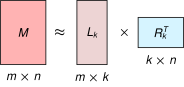](https://mlsysbook.ai/contents/core/optimizations/dcbd6535b09a28528559354f928838baaae7644b.svg "Figure 10: Low-Rank Factorization: Decomposing a matrix into lower-rank approximations reduces the number of parameters needed for storage and computation, enabling efficient model representation. By expressing a matrix a as the product of two smaller matrices, u and v, we transition from storing m \times n parameters to m \times k + k \times n parameters, with k representing the reduced rank. Source: The Clever Machine.")
Figure 10: **Low-Rank Factorization**: Decomposing a matrix into lower-rank approximations reduces the number of parameters needed for storage and computation, enabling efficient model representation. By expressing a matrix \\(a\\) as the product of two smaller matrices, \\(u\\) and \\(v\\), we transition from storing \\(m \\times n\\) parameters to \\(m \\times k + k \\times n\\) parameters, with \\(k\\) representing the reduced rank. Source: The Clever Machine.
LRMF is widely used to enhance the efficiency of machine learning models by reducing parameter redundancy, particularly in fully connected and convolutional layers. In the broader context of machine learning systems, factorization techniques contribute to optimizing model inference speed, storage efficiency, and adaptability to specialized hardware accelerators.
Fully connected layers often contain large weight matrices, making them ideal candidates for factorization. Instead of storing a dense \\(m \\times n\\) weight matrix, LRMF allows for a more compact representation with two smaller matrices of dimensions \\(m \\times k\\) and \\(k \\times n\\), significantly reducing storage and computational costs. This reduction is particularly valuable in cloud-to-edge ML pipelines, where minimizing model size can facilitate real-time execution on embedded devices.
Convolutional layers can also benefit from LRMF by decomposing convolutional filters into separable structures. Techniques such as depthwise-separable convolutions leverage factorization principles to achieve computational efficiency without significant loss in accuracy. These methods align well with hardware-aware optimizations used in modern AI acceleration frameworks.
LRMF has been extensively used in collaborative filtering for recommendation systems. By factorizing user-item interaction matrices, latent factors corresponding to user preferences and item attributes can be extracted, enabling efficient and accurate recommendations. Within large-scale machine learning systems, such optimizations directly impact scalability and performance in production environments.
##### Factorization Efficiency and Challenges
By factorizing a weight matrix into lower-rank components, the number of parameters required for storage is reduced from \\(O(mn)\\) to \\(O(mk + kn)\\), where \\(k\\) is significantly smaller than \\(m, n\\). However, this reduction comes at the cost of an additional matrix multiplication operation during inference, potentially increasing computational latency. In machine learning systems, this trade-off is carefully managed to balance storage efficiency and real-time inference speed.
Choosing an appropriate rank \\(k\\) is a key challenge in LRMF. A smaller \\(k\\) results in greater compression but may lead to significant information loss, while a larger \\(k\\) retains more information but offers limited efficiency gains. Methods such as cross-validation and heuristic approaches are often employed to determine the optimal rank, particularly in large-scale ML deployments where compute and storage constraints vary.
In real-world machine learning applications, datasets may contain noise or missing values, which can affect the quality of factorization. Regularization techniques, such as adding an \\(L\_2\\) penalty, can help mitigate overfitting and improve the robustness of LRMF, ensuring stable performance across different ML system architectures.
Low-rank matrix factorization provides an effective approach for reducing the complexity of machine learning models while maintaining their expressive power. By approximating weight matrices with lower-rank representations, LRMF facilitates efficient inference and model deployment, particularly in resource-constrained environments such as edge computing. Within machine learning systems, factorization techniques contribute to scalable, hardware-aware optimizations that enhance real-world model performance. Despite challenges such as rank selection and computational overhead, LRMF remains a valuable tool for improving efficiency in ML system design and deployment.
#### Tensor Decomposition
While low-rank matrix factorization provides an effective method for compressing large weight matrices in machine learning models, many modern architectures rely on multi-dimensional tensors rather than two-dimensional matrices. Convolutional layers, attention mechanisms, and embedding representations commonly involve multi-way interactions that cannot be efficiently captured using standard matrix factorization techniques. In such cases, tensor decomposition provides a more general approach to reducing model complexity while preserving structural relationships within the data.
[](https://mlsysbook.ai/contents/core/optimizations/85c221e23822ef6d4d0ea443a3a4aec3c3dd5e09.svg "Figure 11: Tensor Decomposition: Multi-dimensional tensors enable compact representations of high-dimensional data by factorizing them into lower-rank components, reducing computational costs and memory requirements compared to direct manipulation of the original tensor. This technique extends matrix factorization to handle the multi-way interactions common in modern machine learning models like convolutional neural networks. Source: [@xinyu].")
Figure 11: **Tensor Decomposition**: Multi-dimensional tensors enable compact representations of high-dimensional data by factorizing them into lower-rank components, reducing computational costs and memory requirements compared to direct manipulation of the original tensor. This technique extends matrix factorization to handle the multi-way interactions common in modern machine learning models like convolutional neural networks. Source: ([Richter and Zhao 2021](https://mlsysbook.ai/contents/core/optimizations/optimizations.html#ref-xinyu)
).
Richter, Joel D., and Xinyu Zhao. 2021. “The Molecular Biology of FMRP: New Insights into Fragile x Syndrome.” _Nature Reviews Neuroscience_ 22 (4): 209–22. [https://doi.org/10.1038/s41583-021-00432-0](https://doi.org/10.1038/s41583-021-00432-0)
.
Tensor decomposition (TD) extends the principles of low-rank factorization to higher-order tensors, allowing large multi-dimensional arrays to be expressed in terms of lower-rank components (see [Figure 11](https://mlsysbook.ai/contents/core/optimizations/optimizations.html#fig-tensor-decomposition)
). Given that tensors frequently appear in machine learning systems as representations of weight parameters, activations, and input features, their direct storage and computation often become impractical. By decomposing these tensors into a set of smaller factors, tensor decomposition significantly reduces memory requirements and computational overhead while maintaining the integrity of the original structure.
Tensor decomposition improves efficiency across various machine learning architectures. In convolutional neural networks, it enables approximation of convolutional kernels with lower-dimensional factors, reducing parameters while preserving representational power. In natural language processing, high-dimensional embeddings can be factorized into more compact representations, leading to faster inference and reduced memory consumption. In hardware acceleration, tensor decomposition helps optimize tensor operations for execution on specialized processors, ensuring efficient utilization of computational resources.
##### Training Mathematics
A tensor is a multi-dimensional extension of a matrix, representing data across multiple axes rather than being confined to two-dimensional structures. In machine learning, tensors naturally arise in various contexts, including the representation of weight parameters, activations, and input features. Given the high dimensionality of these tensors, direct storage and computation often become impractical, necessitating efficient factorization techniques.
Tensor decomposition generalizes the principles of low-rank matrix factorization by approximating a high-order tensor with a set of lower-rank components. Formally, for a given tensor \\(\\mathcal{A} \\in \\mathbb{R}^{m \\times n \\times p}\\), the goal of decomposition is to express \\(\\mathcal{A}\\) in terms of factorized components that require fewer parameters to store and manipulate. This decomposition reduces the memory footprint and computational requirements while retaining the structural relationships present in the original tensor.
Several factorization methods have been developed for tensor decomposition, each suited to different applications in machine learning. One common approach is CANDECOMP/PARAFAC (CP) decomposition, which expresses a tensor as a sum of rank-one components. In CP decomposition, a tensor \\(\\mathcal{A} \\in \\mathbb{R}^{m \\times n \\times p}\\) is approximated as \\\[ \\mathcal{A} \\approx \\sum\_{r=1}^{k} u\_r \\otimes v\_r \\otimes w\_r \\\] where \\(u\_r \\in \\mathbb{R}^{m}\\), \\(v\_r \\in \\mathbb{R}^{n}\\), and \\(w\_r \\in \\mathbb{R}^{p}\\) are factor vectors and \\(k\\) is the rank of the approximation.
Another widely used approach is Tucker decomposition, which generalizes singular value decomposition to tensors by introducing a core tensor \\(\\mathcal{G} \\in \\mathbb{R}^{k\_1 \\times k\_2 \\times k\_3}\\) and factor matrices \\(U \\in \\mathbb{R}^{m \\times k\_1}\\), \\(V \\in \\mathbb{R}^{n \\times k\_2}\\), and \\(W \\in \\mathbb{R}^{p \\times k\_3}\\), such that \\\[ \\mathcal{A} \\approx \\mathcal{G} \\times\_1 U \\times\_2 V \\times\_3 W \\\] where \\(\\times\_i\\) denotes the mode-\\(i\\) tensor-matrix multiplication.
Another method, Tensor-Train (TT) decomposition, factorizes high-order tensors into a sequence of lower-rank matrices, reducing both storage and computational complexity. Given a tensor \\(\\mathcal{A} \\in \\mathbb{R}^{m\_1 \\times m\_2 \\times \\dots \\times m\_d}\\), TT decomposition represents it as a product of lower-dimensional tensor cores \\(\\mathcal{G}^{(i)}\\), where each core \\(\\mathcal{G}^{(i)}\\) has dimensions \\(\\mathbb{R}^{r\_{i-1} \\times m\_i \\times r\_i}\\), and the full tensor is reconstructed as \\\[ \\mathcal{A} \\approx \\mathcal{G}^{(1)} \\times \\mathcal{G}^{(2)} \\times \\dots \\times \\mathcal{G}^{(d)} \\\] where \\(r\_i\\) are the TT ranks.
These tensor decomposition methods play a important role in optimizing machine learning models by reducing parameter redundancy while maintaining expressive power. The next section will examine how these techniques are applied to machine learning architectures and discuss their computational trade-offs.
##### Tensor Decomposition Applications
Tensor decomposition methods are widely applied in machine learning systems to improve efficiency and scalability. By factorizing high-dimensional tensors into lower-rank representations, these methods reduce memory usage and computational requirements while preserving the model’s expressive capacity. This section examines several key applications of tensor decomposition in machine learning, focusing on its impact on convolutional neural networks, natural language processing, and hardware acceleration.
In convolutional neural networks (CNNs), tensor decomposition is used to compress convolutional filters and reduce the number of required operations during inference. A standard convolutional layer contains a set of weight tensors that define how input features are transformed. These weight tensors often exhibit redundancy, meaning they can be decomposed into smaller components without significantly degrading performance. Techniques such as CP decomposition and Tucker decomposition enable convolutional filters to be approximated using lower-rank tensors, reducing the number of parameters and computational complexity of the convolution operation. This form of structured compression is particularly valuable in edge and mobile machine learning applications, where memory and compute resources are constrained.
In natural language processing (NLP), tensor decomposition is commonly applied to embedding layers and attention mechanisms. Many NLP models, including transformers, rely on high-dimensional embeddings to represent words, sentences, or entire documents. These embeddings can be factorized using tensor decomposition to reduce storage requirements without compromising their ability to capture semantic relationships. Similarly, in transformer-based architectures, the self-attention mechanism requires large tensor multiplications, which can be optimized using decomposition techniques to lower the computational burden and accelerate inference.
Hardware acceleration for machine learning also benefits from tensor decomposition by enabling more efficient execution on specialized processors such as GPUs, tensor processing units (TPUs), and field-programmable gate arrays (FPGAs). Many machine learning frameworks include optimizations that leverage tensor decomposition to improve model execution speed and reduce energy consumption. Decomposing tensors into structured low-rank components aligns well with the memory hierarchy of modern hardware accelerators, facilitating more efficient data movement and parallel computation.
Despite these advantages, tensor decomposition introduces certain trade-offs that must be carefully managed. The choice of decomposition method and rank significantly influences model accuracy and computational efficiency. Selecting an overly aggressive rank reduction may lead to excessive information loss, while retaining too many components diminishes the efficiency gains. The factorization process itself can introduce a computational overhead, requiring careful consideration when applying tensor decomposition to large-scale machine learning systems.
##### TD Trade-offs and Challenges
While tensor decomposition provides significant efficiency gains in machine learning systems, it introduces trade-offs that must be carefully managed to maintain model accuracy and computational feasibility. These trade-offs primarily involve the selection of decomposition rank, the computational complexity of factorization, and the stability of factorized representations.
One of the primary challenges in tensor decomposition is determining an appropriate rank for the factorized representation. In low-rank matrix factorization, the rank defines the dimensionality of the factorized matrices, directly influencing the balance between compression and information retention. In tensor decomposition, rank selection becomes even more complex, as different decomposition methods define rank in varying ways. For instance, in CANDECOMP/PARAFAC (CP) decomposition, the rank corresponds to the number of rank-one tensors used to approximate the original tensor. In Tucker decomposition, the rank is determined by the dimensions of the core tensor, while in Tensor-Train (TT) decomposition, the ranks of the factorized components dictate the level of compression. Selecting an insufficient rank can lead to excessive information loss, degrading the model’s predictive performance, whereas an overly conservative rank reduction results in limited compression benefits.
Another key challenge is the computational overhead associated with performing tensor decomposition. The factorization process itself requires solving an optimization problem, often involving iterative procedures such as alternating least squares (ALS) or optimization algorithms such as stochastic gradient descent. These methods can be computationally expensive, particularly for large-scale tensors used in machine learning models. During inference, the need to reconstruct tensors from their factorized components introduces additional matrix and tensor multiplications, which may increase computational latency. The efficiency of tensor decomposition in practice depends on striking a balance between reducing parameter storage and minimizing the additional computational cost incurred by factorized representations.
Numerical stability is another concern when applying tensor decomposition to machine learning models. Factorized representations can suffer from numerical instability, particularly when the original tensor contains highly correlated structures or when decomposition methods introduce ill-conditioned factors. Regularization techniques, such as adding constraints on factor matrices or applying low-rank approximations incrementally, can help mitigate these issues. The optimization process used for decomposition must be carefully tuned to avoid convergence to suboptimal solutions that fail to preserve the important properties of the original tensor.
Despite these challenges, tensor decomposition remains a valuable tool for optimizing machine learning models, particularly in applications where reducing memory footprint and computational complexity is a priority. Advances in adaptive decomposition methods, automated rank selection strategies, and hardware-aware factorization techniques continue to improve the practical utility of tensor decomposition in machine learning. The following section will summarize the key insights gained from low-rank matrix factorization and tensor decomposition, highlighting their role in designing efficient machine learning systems.
##### LRMF vs. TD
Both low-rank matrix factorization and tensor decomposition serve as core techniques for reducing the complexity of machine learning models by approximating large parameter structures with lower-rank representations. While they share the common goal of improving storage efficiency and computational performance, their applications, computational trade-offs, and structural assumptions differ significantly. This section provides a comparative analysis of these two techniques, highlighting their advantages, limitations, and practical use cases in machine learning systems.
One of the key distinctions between LRMF and tensor decomposition lies in the dimensionality of the data they operate on. LRMF applies to two-dimensional matrices, making it particularly useful for compressing weight matrices in fully connected layers or embeddings. Tensor decomposition, on the other hand, extends factorization to multi-dimensional tensors, which arise naturally in convolutional layers, attention mechanisms, and multi-modal learning. This generalization allows tensor decomposition to exploit additional structural properties of high-dimensional data that LRMF cannot capture.
Computationally, both methods introduce trade-offs between storage savings and inference speed. LRMF reduces the number of parameters in a model by factorizing a weight matrix into two smaller matrices, thereby reducing memory footprint while incurring an additional matrix multiplication during inference. In contrast, tensor decomposition further reduces storage by decomposing tensors into multiple lower-rank components, but at the cost of more complex tensor contractions, which may introduce higher computational overhead. The choice between these methods depends on whether the primary constraint is memory storage or inference latency.
[Table 5](https://mlsysbook.ai/contents/core/optimizations/optimizations.html#tbl-lrmf-tensor)
summarizes the key differences between LRMF and tensor decomposition:
Table 5: **Dimensionality & Factorization**: Low-rank matrix factorization (LRMF) and tensor decomposition reduce model storage requirements by representing data with fewer parameters, but introduce computational trade-offs during inference; LRMF applies to two-dimensional matrices, while tensor decomposition extends this approach to multi-dimensional tensors for greater compression potential.
| | | |
| --- | --- | --- |
| **Applicable Data Structure** | Two-dimensional matrices | Multi-dimensional tensors |
| **Compression Mechanism** | Factorizes a matrix into two or more lower-rank matrices | Decomposes a tensor into multiple lower-rank components |
| **Common Methods** | Singular Value Decomposition (SVD), Alternating Least Squares (ALS) | CP Decomposition, Tucker Decomposition, Tensor-Train (TT) |
| **Computational Complexity** | Generally lower, often $ O(mnk) $ for a rank-$ k $ approximation | Higher, due to iterative optimization and tensor contractions |
| **Storage Reduction** | Reduces storage from $ O(mn) $ to $ O(mk + kn) $ | Achieves higher compression but requires more complex storage representations |
| **Inference Overhead** | Requires additional matrix multiplication | Introduces additional tensor operations, potentially increasing inference latency |
| **Primary Use Cases** | Fully connected layers, embeddings, recommendation systems | Convolutional filters, attention mechanisms, multi-modal learning |
| **Implementation Complexity** | Easier to implement, often involves direct factorization methods | More complex, requiring iterative optimization and rank selection |
Despite these differences, LRMF and tensor decomposition are not mutually exclusive. In many machine learning models, both methods can be applied together to optimize different components of the architecture. For example, fully connected layers may be compressed using LRMF, while convolutional kernels and attention tensors undergo tensor decomposition. The choice of technique ultimately depends on the specific characteristics of the model and the trade-offs between storage efficiency and computational complexity.
### Neural Architecture Search
Pruning, knowledge distillation, and other techniques explored in previous sections rely on human expertise to determine optimal model configurations. While these manual approaches have led to significant advancements, selecting optimal architectures requires extensive experimentation, and even experienced practitioners may overlook more efficient designs ([Elsken, Metzen, and Hutter 2019a](https://mlsysbook.ai/contents/core/optimizations/optimizations.html#ref-elsken2019neural)
). Neural Architecture Search (NAS) automates this process by systematically exploring large spaces of possible architectures to identify those that best balance accuracy, computational cost, memory efficiency, and inference latency.
———. 2019a. “Neural Architecture Search.” In _Automated Machine Learning_, 20:63–77. 55. Springer International Publishing. [https://doi.org/10.1007/978-3-030-05318-5\\\_3](https://doi.org/10.1007/978-3-030-05318-5/_3)
.
26 **Hardware-Aware NAS**: MnasNet achieves 78.1% ImageNet accuracy with 315M FLOPs vs. MobileNetV2’s 72.0% with 300M FLOPs. EfficientNet-B0 delivers 77.1% accuracy with 390M FLOPs, 23% better accuracy/FLOP ratio than ResNet-50, enabling 4.9x faster mobile inference.
Zoph, Barret, and Quoc V Le. 2017a. “Neural Architecture Search with Reinforcement Learning.” In _International Conference on Learning Representations (ICLR)_.
[Figure 12](https://mlsysbook.ai/contents/core/optimizations/optimizations.html#fig-nas-flow)
illustrates the NAS process. NAS[26](https://mlsysbook.ai/contents/core/optimizations/optimizations.html#fn26)
operates through three interconnected stages: defining the search space (architectural components and constraints), applying search strategies (reinforcement learning([Zoph and Le 2017a](https://mlsysbook.ai/contents/core/optimizations/optimizations.html#ref-zoph2017neural)
), evolutionary algorithms, or gradient-based methods) to explore candidate architectures, and evaluating performance to ensure discovered designs satisfy accuracy and efficiency objectives. This automation enables the discovery of novel architectures that often match or surpass human-designed models while requiring substantially less expert effort.
[](https://mlsysbook.ai/contents/core/optimizations/7a4cfdd5ac778f9b190c672532e117e4f08f5e23.svg "Figure 12: Neural Architecture Search Flow: Automated NAS techniques iteratively refine model architectures and their weights, jointly optimizing for performance and efficiency, a departure from manual design approaches that rely on human expertise and extensive trial-and-error. This process enables the discovery of novel, high-performing architectures tailored to specific computational constraints.")
Figure 12: **Neural Architecture Search Flow**: Automated NAS techniques iteratively refine model architectures and their weights, jointly optimizing for performance and efficiency, a departure from manual design approaches that rely on human expertise and extensive trial-and-error. This process enables the discovery of novel, high-performing architectures tailored to specific computational constraints.
NAS search strategies employ diverse optimization techniques. Reinforcement learning[27](https://mlsysbook.ai/contents/core/optimizations/optimizations.html#fn27)
treats architecture selection as a sequential decision problem, using accuracy as reward signal. Evolutionary algorithms[28](https://mlsysbook.ai/contents/core/optimizations/optimizations.html#fn28)
evolve populations of architectures through mutation and crossover. Gradient-based methods enable differentiable architecture search, reducing computational cost.
27 **Reinforcement Learning NAS**: Uses RL controller networks to generate architectures, with accuracy as reward signal. Google’s NASNet controller was trained for 22,400 GPU-hours on 800 GPUs, but discovered architectures achieving 82.7% ImageNet accuracy—28% better than human-designed ResNet at similar FLOP budgets.
28 **Evolutionary NAS**: Treats architectures as genes, evolving populations through mutation and crossover. AmoebaNet required 3,150 GPU-days but achieved 83.9% ImageNet accuracy. Real et al.’s evolution approach discovered architectures that matched manually tuned models with 7,000x less human effort.
#### Model Efficiency Encoding
NAS operates in three key stages: defining the search space, exploring candidate architectures, and evaluating their performance. The search space defines the architectural components and constraints that NAS can modify. The search strategy determines how NAS explores possible architectures, selecting promising candidates based on past observations. The evaluation process ensures that the discovered architectures satisfy multiple objectives, including accuracy, efficiency, and hardware suitability.
1. Search Space Definition: This stage establishes the architectural components and constraints NAS can modify, such as the number of layers, convolution types, activation functions, and hardware-specific optimizations. A well-defined search space balances innovation with computational feasibility.
2. Search Strategy: NAS explores the search space using methods such as reinforcement learning, evolutionary algorithms, or gradient-based techniques. These approaches guide the search toward architectures that maximize performance while meeting resource constraints.
3. Evaluation Criteria: Candidate architectures are assessed based on multiple metrics, including accuracy, FLOPs, memory consumption, inference latency, and power efficiency. NAS ensures that the selected architectures align with deployment requirements.
NAS unifies structural design and optimization into a singular, automated framework. The result is the discovery of architectures that are not only highly accurate but also computationally efficient and well-suited for target hardware platforms.
#### Search Space Definition
The first step in NAS is determining the set of architectures it is allowed to explore, known as the search space. The size and structure of this space directly affect how efficiently NAS can discover optimal models. A well-defined search space must be broad enough to allow innovation while remaining narrow enough to prevent unnecessary computation on impractical designs.
A typical NAS search space consists of modular building blocks that define the structure of the model. These include the types of layers available for selection, such as standard convolutions, depthwise separable convolutions, attention mechanisms, and residual blocks. The search space also defines constraints on network depth and width, specifying how many layers the model can have and how many channels each layer should include. NAS considers activation functions, such as ReLU, Swish, or GELU, which influence both model expressiveness and computational efficiency.
Other architectural decisions within the search space include kernel sizes, receptive fields, and skip connections, which impact both feature extraction and model complexity. Some NAS implementations also incorporate hardware-aware optimizations, ensuring that the discovered architectures align with specific hardware, such as GPUs, TPUs, or mobile CPUs.
The choice of search space determines the extent to which NAS can optimize a model. If the space is too constrained, the search algorithm may fail to discover novel and efficient architectures. If it is too large, the search becomes computationally expensive, requiring extensive resources to explore a vast number of possibilities. Striking the right balance ensures that NAS can efficiently identify architectures that improve upon human-designed models.
#### Search Space Exploration
Once the search space is defined, NAS must determine how to explore different architectures effectively. The search strategy guides this process by selecting which architectures to evaluate based on past observations. An effective search strategy must balance exploration (testing new architectures) with exploitation (refining promising designs).
Several methods have been developed to explore the search space efficiently. Reinforcement learning-based NAS formulates the search process as a decision-making problem, where an agent sequentially selects architectural components and receives a reward signal based on the performance of the generated model. Over time, the agent learns to generate better architectures by maximizing this reward. While effective, reinforcement learning-based NAS can be computationally expensive because it requires training many candidate models before converging on an optimal design.
An alternative approach uses evolutionary algorithms, which maintain a population of candidate architectures and iteratively improve them through mutation and selection. Stronger architectures, which possess higher accuracy and efficiency, are retained, while modifications such as changing layer types or filter sizes introduce new variations. This approach has been shown to balance exploration and computational feasibility more effectively than reinforcement learning-based NAS.
More recent methods, such as gradient-based NAS, introduce differentiable parameters that represent architectural choices. Instead of treating architectures as discrete entities, gradient-based methods optimize both model weights and architectural parameters simultaneously using standard gradient descent. This significantly reduces the computational cost of the search, making NAS more practical for real-world applications.
The choice of search strategy has a direct impact on the feasibility of NAS. Early NAS methods that relied on reinforcement learning required weeks of GPU computation to discover a single architecture. More recent methods, particularly those based on gradient-based search, have significantly reduced this cost, making NAS more efficient and accessible.
#### Candidate Architecture Evaluation
Every architecture explored by NAS must be evaluated based on a set of predefined criteria. While accuracy is a core metric, NAS also optimizes for efficiency constraints to ensure that models are practical for deployment. The evaluation process determines whether an architecture should be retained for further refinement or discarded in favor of more promising designs.
The primary evaluation metrics include computational complexity, memory consumption, inference latency, and energy efficiency[29](https://mlsysbook.ai/contents/core/optimizations/optimizations.html#fn29)
. Computational complexity, often measured in FLOPs, determines the overall resource demands of a model. NAS favors architectures that achieve high accuracy while reducing unnecessary computations. Memory consumption, which includes both parameter count and activation storage, ensures that models fit within hardware constraints. For real-time applications, inference latency is a key factor, with NAS selecting architectures that minimize execution time on specific hardware platforms. Finally, some NAS implementations explicitly optimize for power consumption, ensuring that models are suitable for mobile and edge devices.
29 **NAS Evaluation Metrics**: Multi-objective optimization considers accuracy (top-1/top-5), latency (ms on target hardware), memory (MB activations + parameters), and energy (mJ per inference). Pareto-optimal architectures provide 15-40% better efficiency frontiers than manual designs.
30 **FBNet**: Achieves 74.9% ImageNet accuracy with 375M FLOPs and 23ms latency on Samsung S8, 15% faster than MobileNetV2 with comparable accuracy. The latency-aware search uses device-specific lookup tables for actual hardware performance measurement ([B. Wu et al. 2019](https://mlsysbook.ai/contents/core/optimizations/optimizations.html#ref-wu2019fbnet)
).
Wu, Bichen, Kurt Keutzer, Xiaoliang Dai, Peizhao Zhang, Yanghan Wang, Fei Sun, Yiming Wu, Yuandong Tian, Peter Vajda, and Yangqing Jia. 2019. “FBNet: Hardware-Aware Efficient ConvNet Design via Differentiable Neural Architecture Search.” In _2019 IEEE/CVF Conference on Computer Vision and Pattern Recognition (CVPR)_, 10726–34. IEEE. [https://doi.org/10.1109/cvpr.2019.01099](https://doi.org/10.1109/cvpr.2019.01099)
.
For example, FBNet[30](https://mlsysbook.ai/contents/core/optimizations/optimizations.html#fn30)
, a NAS-generated architecture optimized for mobile inference, incorporated latency constraints into the search process.
By integrating these constraints into the search process, NAS systematically discovers architectures that balance accuracy, efficiency, and hardware adaptability. Instead of manually fine-tuning these trade-offs, NAS automates the selection of optimal architectures, ensuring that models are well-suited for real-world deployment scenarios.
#### The NAS Optimization Problem
Neural Architecture Search can be formulated as a bi-level optimization problem that simultaneously searches for the optimal architecture while evaluating its performance. The outer loop searches the architecture space, while the inner loop trains candidate architectures to measure their quality.
Formally, NAS seeks to find the optimal architecture \\(\\alpha^\*\\) from a search space \\(\\mathcal{A}\\) that minimizes validation loss \\(\\mathcal{L}\_{\\text{val}}\\) while respecting deployment constraints \\(C\\) (latency, memory, energy):
\\\[ \\alpha^\* = \\arg\\min\_{\\alpha \\in \\mathcal{A}} \\mathcal{L}\_{\\text{val}}(w^\*(\\alpha), \\alpha) \\quad \\text{subject to} \\quad C(\\alpha) \\leq C\_{\\text{max}} \\\]
where \\(w^\*(\\alpha)\\) represents the optimal weights for architecture \\(\\alpha\\), obtained by minimizing training loss:
\\\[ w^\*(\\alpha) = \\arg\\min\_{w} \\mathcal{L}\_{\\text{train}}(w, \\alpha) \\\]
This formulation reveals the core challenge of NAS: evaluating each candidate architecture requires expensive training to convergence, making exhaustive search infeasible. A search space with just 10 design choices per layer across 20 layers yields \\(10^{20}\\) possible architectures. Training each for 100 epochs would require millions of GPU-years. Efficient NAS methods address this challenge through three key design decisions: defining a tractable search space, employing efficient search strategies, and accelerating architecture evaluation.
#### Search Space Design
The search space defines what architectures NAS can discover. Well-designed search spaces incorporate domain knowledge to focus search on promising regions while remaining flexible enough to discover novel patterns.
**Cell-Based Search Spaces**
Rather than searching entire network architectures, cell-based NAS searches for reusable computational blocks (cells) that can be stacked to form complete networks. For example, a convolutional cell might choose from operations like 3×3 convolution, 5×5 convolution, depthwise separable convolution, max pooling, or identity connections. A simplified cell with 4 nodes and 2 operations per edge yields roughly 10,000 possible cell designs, far more tractable than searching full architectures. EfficientNet uses this approach to discover scalable cell designs that generalize across different model sizes.
**Hardware-Aware Search Spaces**
Hardware-aware NAS extends search spaces to include deployment constraints as first-class objectives. Rather than optimizing solely for accuracy and FLOPs, the search explicitly minimizes actual latency on target hardware (mobile CPUs, GPUs, edge accelerators). MobileNetV3’s search space includes a latency prediction model that estimates inference time for each candidate architecture on Pixel phones without actually deploying them. This hardware-in-the-loop approach ensures discovered architectures run efficiently on real devices rather than just achieving low theoretical FLOP counts.
#### Search Strategies
Search strategies determine how to navigate the architecture space efficiently without exhaustive enumeration. Different strategies make different trade-offs between search cost, architectural diversity, and optimality guarantees, as summarized in [Table 6](https://mlsysbook.ai/contents/core/optimizations/optimizations.html#tbl-nas-strategies)
.
Table 6: **NAS Search Strategy Comparison**: Trade-offs between search efficiency, use cases, and limitations for different NAS approaches. Reinforcement learning offers unconstrained exploration at high cost, evolutionary methods leverage parallelism, and gradient-based approaches achieve dramatic speedups with potential optimality trade-offs.
| | | | |
| --- | --- | --- | --- |
| Reinforcement Learning | 400-1000 GPU-days | Novel domains, unconstrained search | High computational cost |
| Evolutionary Algorithms | 200-500 GPU-days | Parallel infrastructure available | Requires large populations |
| Gradient-Based (DARTS) | 1-4 GPU-days | Limited compute budget | May converge to suboptimal local minima |
Reinforcement learning based NAS treats architecture search as a sequential decision problem where a controller generates architectures and receives accuracy as reward. The controller (typically an LSTM) learns to propose better architectures over time through policy gradient optimization. While this approach discovered groundbreaking architectures like NASNet, the sequential nature limits parallelism and requires hundreds of GPU-days.
Evolutionary algorithms maintain a population of candidate architectures and iteratively apply mutations (changing operations, adding connections) and crossover (combining parent architectures) to generate offspring. Fitness-based selection retains high-performing architectures for the next generation. AmoebaNet used evolution to achieve state-of-the-art results, with massive parallelism amortizing the cost across thousands of workers.
Gradient-based methods like DARTS (Differentiable Architecture Search) represent the search space as a continuous relaxation where all possible operations are weighted combinations. Rather than discrete sampling, DARTS optimizes architecture weights and model weights jointly using gradient descent. By making the search differentiable, DARTS reduces search cost from hundreds to just 1-4 GPU-days, though the continuous relaxation may miss discrete architectural patterns that discrete search methods discover.
#### NAS in Practice
Hardware-aware NAS moves beyond FLOPs as a proxy for efficiency, directly optimizing for actual deployment metrics. MnasNet’s search incorporates a latency prediction model trained on thousands of architecture-latency pairs measured on actual mobile phones. The search objective combines accuracy and latency through a weighted product:
\\\[ \\text{Reward}(\\alpha) = \\text{Accuracy}(\\alpha) \\times \\left(\\frac{L(\\alpha)}{L\_{\\text{target}}}\\right)^\\beta \\\]
where \\(L(\\alpha)\\) is measured latency, \\(L\_{\\text{target}}\\) is the latency constraint, and \\(\\beta\\) controls the accuracy-latency trade-off. This formulation penalizes architectures that exceed latency targets while rewarding those that achieve high accuracy within the budget. MnasNet discovered that inverted residuals with varying expansion ratios achieve better accuracy-latency trade-offs than uniform expansion, a design insight that manual exploration likely would have missed.
#### When to Use NAS
Neural Architecture Search is a powerful tool, but its significant computational cost demands careful consideration of when the investment is justified.
NAS becomes worthwhile when dealing with novel hardware platforms with unique constraints (new accelerator architectures, extreme edge devices) where existing architectures are poorly optimized. It also makes sense for deployment at massive scale (billions of inferences) where even 1-2% efficiency improvements justify the upfront search cost, or when multiple deployment configurations require architecture families (cloud, edge, mobile) that can amortize one search across many variants.
Conversely, avoid NAS when working with standard deployment constraints (e.g., ResNet-50 accuracy on NVIDIA GPUs) where well-optimized architectures already exist. Similarly, if the compute budget is limited (less than 100 GPU-days available), even efficient NAS methods like DARTS become infeasible. Rapidly changing requirements also make NAS impractical, as architecture selection may become obsolete before the search completes.
For most practitioners, starting with existing NAS-discovered architectures (EfficientNet, MobileNetV3, MnasNet) provides better ROI than running NAS from scratch. These architectures are highly tuned and generalize well across tasks. Reserve custom NAS for scenarios with truly novel constraints or deployment scales that justify the investment.
#### Architecture Examples
NAS has been successfully used to design several state-of-the-art architectures that outperform manually designed models in terms of efficiency and accuracy. These architectures illustrate how NAS integrates scaling optimization, computation reduction, memory efficiency, and hardware-aware design into an automated process.
One of the most well-known NAS-generated models is EfficientNet, which was discovered using a NAS framework that searched for the most effective combination of depth, width, and resolution scaling. Unlike traditional scaling strategies that independently adjust these factors, NAS optimized the model using compound scaling, which applies a fixed set of scaling coefficients to ensure that the network grows in a balanced way. EfficientNet achieves higher accuracy with fewer parameters and lower FLOPs than previous architectures, making it ideal for both cloud and mobile deployment.
Another key example is MobileNetV3, which used NAS to optimize its network structure for mobile hardware. The search process led to the discovery of inverted residual blocks with squeeze-and-excitation layers, which improve accuracy while reducing computational cost. NAS also selected optimized activation functions and efficient depthwise separable convolutions, leading to a \\(5\\times\\) reduction in FLOPs compared to earlier MobileNet versions.
FBNet, another NAS-generated model, was specifically optimized for real-time inference on mobile CPUs. Unlike architectures designed for general-purpose acceleration, FBNet’s search process explicitly considered latency constraints during training, ensuring that the final model runs efficiently on low-power hardware. Similar approaches have been used in TPU-optimized NAS models, where the search process is guided by hardware-aware cost functions to maximize parallel execution efficiency.
NAS has also been applied beyond convolutional networks. NAS-BERT explores transformer-based architectures, searching for efficient model structures that retain strong natural language understanding capabilities while reducing compute and memory overhead. NAS has been particularly useful in designing efficient vision transformers (ViTs) by automatically discovering lightweight attention mechanisms tailored for edge AI applications.
Each of these NAS-generated models demonstrates how automated architecture search can uncover novel efficiency trade-offs that may not be immediately intuitive to human designers. Explicit encoding of efficiency constraints into the search process enables NAS to systematically produce architectures that are more computationally efficient, memory-friendly, and hardware-adapted than those designed manually ([Radosavovic et al. 2020](https://mlsysbook.ai/contents/core/optimizations/optimizations.html#ref-radosavovic2020designing)
).
Radosavovic, Ilija, Raj Prateek Kosaraju, Ross Girshick, Kaiming He, and Piotr Dollar. 2020. “Designing Network Design Spaces.” In _2020 IEEE/CVF Conference on Computer Vision and Pattern Recognition (CVPR)_, 10428–36. IEEE. [https://doi.org/10.1109/cvpr42600.2020.01044](https://doi.org/10.1109/cvpr42600.2020.01044)
.
Model representation optimization has delivered substantial improvements. Through structured pruning and knowledge distillation, we transformed a 440MB BERT-Base model ([Devlin et al. 2018](https://mlsysbook.ai/contents/core/optimizations/optimizations.html#ref-devlin2018bert)
) into a 110MB variant, decreasing memory footprint by 75% with only 0.8% accuracy loss. The pruned model eliminates 40% of attention heads and intermediate dimensions, significantly reducing parameter count. This success creates a natural question: with the model structurally optimized, why does mobile deployment still fail to meet our 50ms latency target, consistently running at 120ms?
Profiling reveals the answer. While we eliminated 75% of parameters, each remaining matrix multiplication still uses 32-bit floating-point operations (FP32). The 27.5 million remaining parameters consume excessive memory bandwidth: loading weights from DRAM to compute units dominates execution time. The model structure is optimized, but numerical representation is not. Each parameter occupies 4 bytes, and limited mobile memory bandwidth (25-35 GB/s versus 900 GB/s on server GPUs) creates a bottleneck that structural optimization alone cannot resolve.
This illustrates why model representation optimization represents only the first dimension of a comprehensive efficiency strategy. Representation techniques modify what computations are performed (which operations, which parameters, which layers execute). Numerical precision optimization, the second dimension, changes how those computations are executed by reducing the numerical fidelity of weights, activations, and arithmetic operations. Moving from 32-bit to 8-bit representations reduces memory traffic by 4x and enables specialized integer arithmetic units that execute 4-8x faster than floating-point equivalents on mobile processors.
These precision optimizations work synergistically with representation optimizations. The pruned 110MB BERT model, when further quantized to INT8 precision, shrinks to 28MB while inference latency drops to 45ms, finally meeting the deployment target. The quantization provides the missing piece: structural efficiency (fewer parameters) combined with numerical efficiency (lower precision per parameter) delivers compound benefits that neither technique achieves alone.
**Self-Check: Question 1.6**
1. Which of the following best describes the purpose of gradient checkpointing in neural network optimization?
1. To reduce memory usage by recomputing intermediate activations during backpropagation.
2. To improve model accuracy by increasing the number of parameters.
3. To enhance computational speed by parallelizing model training.
4. To eliminate redundant parameters through pruning.
2. Explain the trade-offs involved in model pruning and how it affects deployment in different environments.
3. The process of systematically removing redundant parameters from a neural network while preserving accuracy is known as \_\_\_\_. This technique reduces model size and computational cost.
4. What is a primary advantage of using parallel processing patterns in machine learning model optimization?
1. It increases the number of parameters in the model.
2. It reduces the need for gradient checkpointing.
3. It allows for faster training by utilizing multiple cores simultaneously.
4. It eliminates the need for model pruning.
[See Answers →](https://mlsysbook.ai/contents/core/optimizations/optimizations.html#quiz-answer-sec-model-optimizations-structural-model-optimization-methods-ca9e)
Quantization and Precision Optimization
---------------------------------------
**Definition:** Quantization
**_Quantization_** is a model compression technique that reduces _numerical precision_ of weights and activations from floating-point to lower-bit representations, decreasing _model size_ and _computational cost_ with minimal accuracy loss.
While model representation optimization determines what computations are performed, the efficiency of those computations depends critically on numerical precision—the second dimension of our optimization framework.
Numerical precision determines how weights and activations are represented during computation, directly affecting memory usage, computational efficiency, and power consumption. Many state-of-the-art models use high-precision floating-point formats like FP32 (32-bit floating point), which offer numerical stability and high accuracy ([Gupta et al. 2015](https://mlsysbook.ai/contents/core/optimizations/optimizations.html#ref-gupta2015deep)
) but increase storage requirements, memory bandwidth usage, and power consumption. Modern AI accelerators include dedicated hardware for low-precision computation, allowing FP16 and INT8 operations to run at significantly higher throughput than FP32 ([Y. E. Wang, Wei, and Brooks 2019](https://mlsysbook.ai/contents/core/optimizations/optimizations.html#ref-wang2019benchmarking)
). Reducing precision introduces quantization error that can degrade accuracy, with tolerance depending on model architecture, dataset properties, and hardware support.
Gupta, Suyog, Ankur Agrawal, Kailash Gopalakrishnan, and Pritish Narayanan. 2015. “Deep Learning with Limited Numerical Precision.” In _International Conference on Machine Learning_, 1737–46. PMLR.
Wang, Yu Emma, Gu-Yeon Wei, and David Brooks. 2019. “Benchmarking TPU, GPU, and CPU Platforms for Deep Learning.” _arXiv Preprint arXiv:1907.10701_, July. [http://arxiv.org/abs/1907.10701v4](http://arxiv.org/abs/1907.10701v4)
.
The relationship between precision reduction and system performance proves more complex than hardware specifications suggest. While aggressive precision reduction (e.g., INT8) can deliver impressive chip-level performance improvements (often 4x higher TOPS compared to FP32), these micro-benchmarks may not translate to end-to-end system benefits. Ultra-low precision training often requires longer convergence times, complex mixed-precision orchestration, and sophisticated accuracy recovery techniques that can offset hardware speedups. Precision conversions between numerical formats introduce computational overhead and memory bandwidth pressure that chip-level benchmarks typically ignore. Balanced approaches, such as FP16 mixed-precision training, often provide optimal compromise between hardware efficiency and training convergence, avoiding the systems-level complexity that accompanies more aggressive quantization strategies.
This section examines precision optimization techniques across three complexity tiers: post-training quantization for rapid deployment, quantization-aware training for production systems, and extreme quantization (binarization and ternarization) for resource-constrained environments. We explore trade-offs between precision formats, hardware-software co-design considerations, and methods for minimizing accuracy degradation while maximizing efficiency gains.
### Precision and Energy
Efficient numerical representations enable significant reductions in storage requirements, computation latency, and power usage, making them particularly beneficial for mobile AI, embedded systems, and cloud inference. Precision levels can be tuned to specific hardware capabilities, maximizing throughput on AI accelerators such as GPUs, TPUs, NPUs, and edge AI chips.
#### Energy Costs
Beyond computational and memory benefits, the energy costs associated with different numerical precisions further highlight the benefits of reducing precision. As shown in [Figure 13](https://mlsysbook.ai/contents/core/optimizations/optimizations.html#fig-quantized-energy)
, performing a 32-bit floating-point addition (FAdd) consumes approximately 0.9 pJ, whereas a 16-bit floating-point addition only requires 0.4 pJ. Similarly, a 32-bit integer addition costs 0.1 pJ, while an 8-bit integer addition is significantly lower at just 0.03 pJ. These savings compound when considering large-scale models operating across billions of operations, supporting the sustainability goals outlined in **[Chapter 18: Sustainable AI](https://mlsysbook.ai/contents/core/sustainable_ai/sustainable_ai.html#sec-sustainable-ai)
**. The energy efficiency gained through quantization also enhances the security posture discussed in **[Chapter 15: Security & Privacy](https://mlsysbook.ai/contents/core/privacy_security/privacy_security.html#sec-security-privacy)
** by reducing the computational resources available to potential attackers.
[](https://mlsysbook.ai/contents/core/optimizations/de8d00428fde3659252984b9b52801e879672837.svg "Figure 13: Energy Costs: Lower precision reduces computational energy, illustrating trade-offs in model accuracy. Machine learning systems can optimize efficiency by reducing floating-point operations from 32-bit to 16-bit or even lower for significant savings. Source: IEEE spectrum.")
Figure 13: **Energy Costs**: Lower precision reduces computational energy, illustrating trade-offs in model accuracy. Machine learning systems can optimize efficiency by reducing floating-point operations from 32-bit to 16-bit or even lower for significant savings. Source: IEEE spectrum.
Beyond direct compute savings, reducing numerical precision has a significant impact on memory energy consumption, which often dominates total system power. Lower-precision representations reduce data storage requirements and memory bandwidth usage, leading to fewer and more efficient memory accesses. This is important because accessing memory, particularly off-chip DRAM, is far more energy-intensive than performing arithmetic operations. For instance, DRAM accesses require orders of magnitude more energy (1.3–2.6 nJ) compared to cache accesses (e.g., 10 pJ for an 8 KB L1 cache access). The breakdown of instruction energy underscores the cost of moving data within the memory hierarchy, where an instruction’s total energy can be significantly impacted by memory access patterns[31](https://mlsysbook.ai/contents/core/optimizations/optimizations.html#fn31)
.
31 **Energy Efficiency Metrics**: INT8 quantization reduces energy consumption by 4-8x over FP32 on supported hardware. MobileNetV2 INT8 consumes 47mJ vs. 312mJ FP32 per inference on Cortex-A75. ResNet-50 on TPU v4 achieves 0.9 TOPS/Watt vs. 0.3 TOPS/Watt on V100 GPU.
By reducing numerical precision, models can not only execute computations more efficiently but also reduce data movement, leading to lower overall energy consumption. This is particularly important for hardware accelerators and edge devices, where memory bandwidth and power efficiency are key constraints.
#### Performance Gains
[Figure 14](https://mlsysbook.ai/contents/core/optimizations/optimizations.html#fig-quantization_impact)
illustrates the impact of quantization on both inference time and model size using a stacked bar chart with a dual-axis representation. The left bars in each category show inference time improvements when moving from FP32 to INT8, while the right bars depict the corresponding reduction in model size. The results indicate that quantized models achieve up to \\(4\\times\\) faster inference while reducing storage requirements by a factor of \\(4\\times\\), making them highly suitable for deployment in resource-constrained environments.
[](https://mlsysbook.ai/contents/core/optimizations/2469f7946d97ab5c299210f470f87a52928b1e16.svg "Figure 14: Quantization Impact: Moving from FP32 to INT8 reduces inference time by up to 4 times while decreasing model size by a factor of 4, making models more efficient for resource-constrained environments.")
Figure 14: **Quantization Impact**: Moving from FP32 to INT8 reduces inference time by up to 4 times while decreasing model size by a factor of 4, making models more efficient for resource-constrained environments.
However, reducing numerical precision introduces trade-offs. Lower-precision formats can lead to numerical instability and quantization noise, potentially affecting model accuracy. Some architectures, such as large transformer-based NLP models, tolerate quantization well, whereas others may experience significant degradation. Thus, selecting the appropriate numerical precision requires balancing accuracy constraints, hardware support, and efficiency gains.
[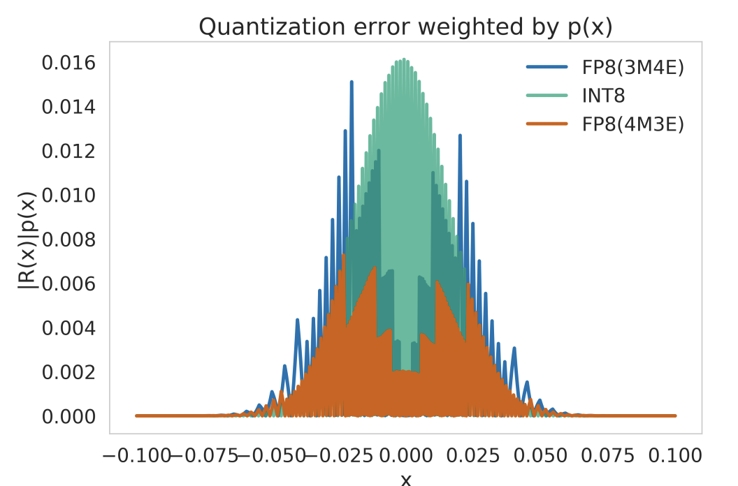](https://mlsysbook.ai/contents/core/optimizations/images/png/modeloptimization_quant_hist.png "Figure 15: Quantization error weighted by p(x).")
Figure 15: Quantization error weighted by p(x).
[Figure 15](https://mlsysbook.ai/contents/core/optimizations/optimizations.html#fig-quantization)
illustrates the quantization error weighted by the probability distribution of values, comparing different numerical formats (FP8 variants and INT8). The error distribution highlights how different formats introduce varying levels of quantization noise across the range of values, which in turn influences model accuracy and stability.
### Numeric Encoding and Storage
The representation of numerical data in machine learning systems extends beyond precision levels to encompass encoding formats and storage mechanisms, both of which significantly influence computational efficiency. The encoding of numerical values determines how floating-point and integer representations are stored in memory and processed by hardware, directly affecting performance in machine learning workloads. As machine learning models grow in size and complexity, optimizing numeric encoding becomes increasingly important for ensuring efficiency, particularly on specialized hardware accelerators ([Mellempudi et al. 2019](https://mlsysbook.ai/contents/core/optimizations/optimizations.html#ref-mellempudi2019mixed)
).
Mellempudi, Naveen, Sudarshan Srinivasan, Dipankar Das, and Bharat Kaul. 2019. “Mixed Precision Training with 8-Bit Floating Point.” _arXiv Preprint arXiv:1905.12334_, May. [http://arxiv.org/abs/1905.12334v1](http://arxiv.org/abs/1905.12334v1)
.
Floating-point representations, which are widely used in machine learning, follow the [IEEE 754 standard](https://standards.ieee.org/standard/754-2019.html)
, defining how numbers are represented using a combination of sign, exponent, and mantissa (fraction) bits. Standard formats such as FP32 (single precision) and FP64 (double precision) provide high accuracy but demand significant memory and computational resources. To enhance efficiency, reduced-precision formats such as FP16, [bfloat16](https://cloud.google.com/tpu/docs/bfloat16)
, and [FP8](https://arxiv.org/abs/2209.05433)
have been introduced, offering lower storage requirements while maintaining sufficient numerical range for machine learning computations. Unlike FP16, which allocates more bits to the mantissa, bfloat16 retains the same exponent size as FP32, allowing it to represent a wider dynamic range while reducing precision in the fraction. This characteristic makes bfloat16 particularly effective for machine learning training, where maintaining dynamic range is important for stable gradient updates.
Integer-based representations, including INT8 and INT4, further reduce storage and computational overhead by eliminating the need for exponent and mantissa encoding. These formats are commonly used in quantized inference, where model weights and activations are converted to discrete integer values to accelerate computation and reduce power consumption. The deterministic nature of integer arithmetic simplifies execution on hardware, making it particularly well-suited for edge AI and mobile devices. At the extreme end, binary and ternary representations restrict values to just one or two bits, leading to significant reductions in memory footprint and power consumption. However, such aggressive quantization can degrade model accuracy unless complemented by specialized training techniques or architectural adaptations.
Emerging numeric formats seek to balance the trade-off between efficiency and accuracy. [TF32](https://blogs.nvidia.com/blog/2020/05/14/tensorfloat-32-precision-format/)
, introduced by NVIDIA for Ampere GPUs, modifies FP32 by reducing the mantissa size while maintaining the exponent width, allowing for faster computations with minimal precision loss. Similarly, FP8, which is gaining adoption in AI accelerators, provides an even lower-precision floating-point alternative while retaining a structure that aligns well with machine learning workloads ([Micikevicius et al. 2022](https://mlsysbook.ai/contents/core/optimizations/optimizations.html#ref-micikevicius2022fp8)
). Alternative formats such as [Posit](https://ieeexplore.ieee.org/document/9399648)
, [Flexpoint](https://arxiv.org/abs/1711.02213)
, and [BF16ALT](https://developer.arm.com/documentation/ddi0596/2020-12/SIMD-FP-Instructions/BFMLALB--BFMLALT--vector---BFloat16-floating-point-widening-multiply-add-long--vector--)
are also being explored for their potential advantages in numerical stability and hardware adaptability.
Micikevicius, Paulius, Dusan Stosic, Neil Burgess, Marius Cornea, Pradeep Dubey, Richard Grisenthwaite, Sangwon Ha, et al. 2022. “FP8 Formats for Deep Learning.” _arXiv Preprint arXiv:2209.05433_, September. [http://arxiv.org/abs/2209.05433v2](http://arxiv.org/abs/2209.05433v2)
.
The efficiency of numeric encoding is further influenced by how data is stored and accessed in memory. AI accelerators optimize memory hierarchies to maximize the benefits of reduced-precision formats, using specialized hardware such as tensor cores, matrix multiply units (MMUs), and vector processing engines to accelerate lower-precision computations. On these platforms, data alignment, memory tiling, and compression techniques play a important role in ensuring that reduced-precision computations deliver tangible performance gains.
As machine learning systems evolve, numeric encoding and storage strategies will continue to adapt to meet the demands of large-scale models and diverse hardware environments. The ongoing development of precision formats tailored for AI workloads highlights the importance of co-designing numerical representations with underlying hardware capabilities, ensuring that machine learning models achieve optimal performance while minimizing computational costs.
### Numerical Format Comparison
[Table 7](https://mlsysbook.ai/contents/core/optimizations/optimizations.html#tbl-numerics)
compares commonly used numerical precision formats in machine learning, highlighting their trade-offs in storage efficiency, computational speed, and energy consumption. Emerging formats like FP8 and TF32 have been introduced to further optimize performance, particularly on AI accelerators.
Table 7: Comparison of numerical precision formats.
| | | | | | |
| --- | --- | --- | --- | --- | --- |
| **FP32 (Single-Precision Floating Point)** | 32-bit | Baseline (1×) | Baseline (1×) | High | Training & inference (general-purpose) |
| **FP16 (Half-Precision Floating Point)** | 16-bit | 2× smaller | 2× faster on FP16-optimized hardware | Lower | Accelerated training, inference (NVIDIA Tensor Cores, TPUs) |
| **bfloat16 (Brain Floating Point)** | 16-bit | 2× smaller | Similar speed to FP16, better dynamic range | Lower | Training on TPUs, transformer-based models |
| **TF32 (TensorFloat-32)** | 19-bit | Similar to FP16 | Up to 8× faster on NVIDIA Ampere GPUs | Lower | Training on NVIDIA GPUs |
| **FP8 (Floating-Point 8-bit)** | 8-bit | 4× smaller | Faster than INT8 in some cases | Significantly lower | Efficient training/inference (H100, AI accelerators) |
| **INT8 (8-bit Integer)** | 8-bit | 4× smaller | 4–8× faster than FP32 | Significantly lower | Quantized inference (Edge AI, mobile AI, NPUs) |
| **INT4 (4-bit Integer)** | 4-bit | 8× smaller | Hardware-dependent | Extremely low | Ultra-low-power AI, experimental quantization |
| **Binary/Ternary (1-bit / 2-bit)** | 1–2-bit | 16–32× smaller | Highly hardware-dependent | Lowest | Extreme efficiency (binary/ternary neural networks) |
FP16 and bfloat16 formats provide moderate efficiency gains while preserving model accuracy. Many AI accelerators, such as NVIDIA Tensor Cores and TPUs, include dedicated support for FP16 computations, enabling \\(2\\times\\) faster matrix operations compared to FP32. BFloat16, in particular, retains the same 8-bit exponent as FP32 but with a reduced 7-bit mantissa, allowing it to maintain a similar dynamic range (~\\(10^{-38}\\) to \\(10^{38}\\)) while sacrificing precision. In contrast, FP16, with its 5-bit exponent and 10-bit mantissa, has a significantly reduced dynamic range (~\\(10^{-5}\\) to \\(10^5\\)), making it more suitable for inference rather than training. Since BFloat16 preserves the exponent size of FP32, it better handles extreme values encountered during training, whereas FP16 may struggle with underflow or overflow. This makes BFloat16 a more robust alternative for deep learning workloads that require a wide dynamic range.
[Figure 16](https://mlsysbook.ai/contents/core/optimizations/optimizations.html#fig-3float)
highlights these differences, showing how bit-width allocations impact the trade-offs between precision and numerical range.
[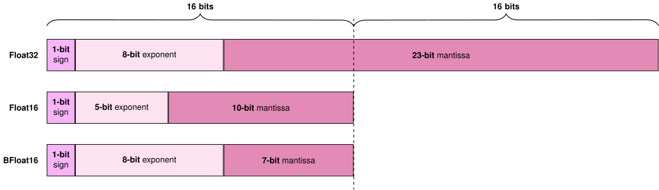](https://mlsysbook.ai/contents/core/optimizations/0c495c39d993058d2b044c479e53d3e31ca18513.svg "Figure 16: Floating-Point Precision: Reduced-precision formats like FP16 and bfloat16 trade off numerical range for computational efficiency and memory savings. Bfloat16 maintains the exponent size of FP32, preserving its dynamic range and suitability for training, while FP16’s smaller exponent limits its use to inference or carefully scaled training scenarios.")
Figure 16: **Floating-Point Precision**: Reduced-precision formats like FP16 and bfloat16 trade off numerical range for computational efficiency and memory savings. Bfloat16 maintains the exponent size of FP32, preserving its dynamic range and suitability for training, while FP16’s smaller exponent limits its use to inference or carefully scaled training scenarios.
INT8 precision offers more aggressive efficiency improvements, particularly for inference workloads. Many quantized models use INT8 for inference, reducing storage by \\(4\\times\\) while accelerating computation by 4–8\\(\\times\\) on optimized hardware. INT8 is widely used in mobile and embedded AI, where energy constraints are significant.
Binary and ternary networks represent the extreme end of quantization, where weights and activations are constrained to 1-bit (binary) or 2-bit (ternary) values. This results in massive storage and energy savings, but model accuracy often degrades significantly unless specialized architectures are used.
### Precision Reduction Trade-offs
Reducing numerical precision in machine learning systems offers significant gains in efficiency, including lower memory requirements, reduced power consumption, and increased computational throughput. However, these benefits come with trade-offs, as lower-precision representations introduce numerical error and quantization noise, which can affect model accuracy. The extent of this impact depends on multiple factors, including the model architecture, the dataset, and the specific precision format used.
Models exhibit varying levels of tolerance to quantization. Large-scale architectures, such as convolutional neural networks and transformer-based models, often retain high accuracy even when using reduced-precision formats such as bfloat16 or INT8. In contrast, smaller models or those trained on tasks requiring high numerical precision may experience greater degradation in performance. Not all layers within a neural network respond equally to precision reduction. Certain layers, such as batch normalization and attention mechanisms, may be more sensitive to numerical precision than standard feedforward layers. As a result, techniques such as mixed-precision training, where different layers operate at different levels of precision, can help maintain accuracy while optimizing computational efficiency.
Hardware support is another important factor in determining the effectiveness of precision reduction. AI accelerators, including GPUs, TPUs, and NPUs, are designed with dedicated low-precision arithmetic units that enable efficient computation using FP16, bfloat16, INT8, and, more recently, FP8. These architectures exploit reduced precision to perform high-throughput matrix operations, improving both speed and energy efficiency. In contrast, general-purpose CPUs often lack specialized hardware for low-precision computations, limiting the potential benefits of numerical quantization. The introduction of newer floating-point formats, such as TF32 for NVIDIA GPUs and FP8 for AI accelerators, seeks to optimize the trade-off between precision and efficiency, offering an alternative for hardware that is not explicitly designed for extreme quantization.
In addition to hardware constraints, reducing numerical precision impacts power consumption. Lower-precision arithmetic reduces the number of required memory accesses and simplifies computational operations, leading to lower overall energy use. This is particularly advantageous for energy-constrained environments such as mobile devices and edge AI systems. At the extreme end, ultra-low precision formats, including INT4 and binary/ternary representations, provide significant reductions in power and memory usage. However, these formats often require specialized architectures to compensate for the accuracy loss associated with such aggressive quantization.
To mitigate accuracy loss associated with reduced precision, various quantization strategies can be employed. Ultimately, selecting the appropriate numerical precision for a given machine learning model requires balancing efficiency gains against accuracy constraints. This selection depends on the model’s architecture, the computational requirements of the target application, and the underlying hardware’s support for low-precision operations. By using advancements in both hardware and software optimization techniques, practitioners can effectively integrate lower-precision numerics into machine learning pipelines, maximizing efficiency while maintaining performance.
### Precision Reduction Strategies
Reducing numerical precision is an important optimization technique for improving the efficiency of machine learning models. By lowering the bit-width of weights and activations, models can reduce memory footprint, improve computational throughput, and decrease power consumption. However, naive quantization can introduce quantization errors, leading to accuracy degradation. To address this, different precision reduction strategies have been developed, allowing models to balance efficiency gains while preserving predictive performance.
Quantization techniques can be applied at different stages of a model’s lifecycle. Post-training quantization reduces precision after training, making it a simple and low-cost approach for optimizing inference. Quantization-aware training incorporates quantization effects into the training process, enabling models to adapt to lower precision and retain higher accuracy. Mixed-precision training leverages hardware support to dynamically assign precision levels to different computations, optimizing execution efficiency without sacrificing accuracy.
To help navigate this increasing complexity, [Figure 17](https://mlsysbook.ai/contents/core/optimizations/optimizations.html#fig-quantization-roadmap)
organizes quantization techniques into three progressive tiers based on implementation complexity, resource requirements, and target use cases.
[](https://mlsysbook.ai/contents/core/optimizations/21a6d5d2509cd55f72c710456c91e3ffca6ba718.svg "Figure 17: Quantization Complexity Roadmap: Three progressive tiers of quantization techniques, from foundational approaches suitable for quick deployment to research frontier methods for extreme resource constraints, reflecting increasing implementation effort, resource requirements, and potential accuracy trade-offs.")
Figure 17: **Quantization Complexity Roadmap**: Three progressive tiers of quantization techniques, from foundational approaches suitable for quick deployment to research frontier methods for extreme resource constraints, reflecting increasing implementation effort, resource requirements, and potential accuracy trade-offs.
#### Post-Training Quantization
Quantization is the specific algorithmic technique that enables significant memory bandwidth reduction when addressing the memory wall. These quantization methods provide standardized APIs across different platforms, showing exactly how to implement the efficiency principles established earlier.
Post-training quantization (PTQ) reduces numerical precision after training, converting weights and activations from high-precision formats (FP32) to lower-precision representations (INT8 or FP16) without retraining ([Jacob et al. 2018a](https://mlsysbook.ai/contents/core/optimizations/optimizations.html#ref-jacob2018quantization)
). This achieves smaller model sizes, faster computation, and reduced energy consumption, making it practical for resource-constrained environments such as mobile devices, edge AI systems, and cloud inference platforms ([H. Wu et al. 2020](https://mlsysbook.ai/contents/core/optimizations/optimizations.html#ref-wu2020integer)
).
PTQ’s key advantage is low computational cost—it requires no retraining or access to training data. However, reducing precision introduces quantization error that can degrade accuracy, particularly for tasks requiring fine-grained numerical precision. Machine learning frameworks (TensorFlow Lite, ONNX Runtime, PyTorch) provide built-in PTQ support.
##### PTQ Functionality
PTQ converts a trained model’s weights and activations from high-precision floating-point representations (e.g., FP32) to lower-precision formats (e.g., INT8 or FP16). This process reduces the memory footprint of the model, accelerates inference, and lowers power consumption. However, since lower-precision formats have a smaller numerical range, quantization introduces rounding errors, which can impact model accuracy.
The core mechanism behind PTQ is scaling and mapping high-precision values into a reduced numerical range. A widely used approach is uniform quantization, which maps floating-point values to discrete integer levels using a consistent scaling factor. In uniform quantization, the interval between each quantized value is constant, simplifying implementation and ensuring efficient execution on hardware. The quantized value \\(q\\) is computed as: \\\[ q = \\text{round} \\left(\\frac{x}{s} \\right) \\\] where:
* \\(q\\) is the quantized integer representation,
* \\(x\\) is the original floating-point value,
* \\(s\\) is a scaling factor that maps the floating-point range to the available integer range.
[Listing 2](https://mlsysbook.ai/contents/core/optimizations/optimizations.html#lst-quantization_example)
demonstrates uniform quantization from FP32 to INT8.
Listing 2: **Uniform Quantization**: Converts FP32 weights to INT8 format, achieving 4x memory reduction while measuring quantization error.
import torch
# Original FP32 weights
weights_fp32 = torch.tensor(
[0.127, -0.084, 0.392, -0.203], dtype=torch.float32
)
print(f"Original FP32: {weights_fp32}")
print(f"Memory per weight: 32 bits")
# Simple uniform quantization to INT8 (-128 to 127)
# Step 1: Find scale factor
max_val = weights_fp32.abs().max()
scale = max_val / 127 # 127 is max positive INT8 value
# Step 2: Quantize using our formula q = round(x/s)
weights_int8 = torch.round(weights_fp32 / scale).to(torch.int8)
print(f"Quantized INT8: {weights_int8}")
print(f"Memory per weight: 8 bits (reduced from 32)")
# Step 3: Dequantize to verify
weights_dequantized = weights_int8.float() * scale
print(f"Dequantized: {weights_dequantized}")
print(
f"Quantization error: "
f"{(weights_fp32 - weights_dequantized).abs().mean():.6f}"
)
This example demonstrates the compression from 32 bits to 8 bits per weight, with minimal quantization error.
For example, in INT8 quantization, the model’s floating-point values (typically ranging from \\(\[-r, r\]\\)) are mapped to an integer range of \\(\[-128, 127\]\\). The scaling factor ensures that the most significant information is retained while reducing precision loss. Once the model has been quantized, inference is performed using integer arithmetic, which is significantly more efficient than floating-point operations on many hardware platforms ([Gholami et al. 2021](https://mlsysbook.ai/contents/core/optimizations/optimizations.html#ref-gholami2021survey)
). However, due to rounding errors and numerical approximation, quantized models may experience slight accuracy degradation compared to their full-precision counterparts.
Once the model has been quantized, inference is performed using integer arithmetic, which is significantly more efficient than floating-point operations on many hardware platforms. However, due to rounding errors and numerical approximation, quantized models may experience slight accuracy degradation compared to their full-precision counterparts.
In addition to uniform quantization, non-uniform quantization can be employed to preserve accuracy in certain scenarios. Unlike uniform quantization, which uses a consistent scaling factor, non-uniform quantization assigns finer-grained precision to numerical ranges that are more densely populated. This approach can be beneficial for models with weight distributions that concentrate around certain values, as it allows more details to be retained where it matters most. However, non-uniform quantization typically requires more complex calibration and may involve additional computational overhead. While it is not as commonly used as uniform quantization in production environments, non-uniform techniques can be effective for preserving accuracy in models that are particularly sensitive to precision changes.
PTQ is particularly effective for computer vision models, where CNNs often tolerate quantization well. However, models that rely on small numerical differences, such as NLP transformers or speech recognition models, may require additional tuning or alternative quantization techniques, including non-uniform strategies, to retain performance.
##### Calibration
An important aspect of PTQ is the calibration step, which involves selecting the most effective clipping range \[\\(\\alpha\\), \\(\\beta\\)\] for quantizing model weights and activations. During PTQ, the model’s weights and activations are converted to lower-precision formats (e.g., INT8), but the effectiveness of this reduction depends heavily on the chosen quantization range. Without proper calibration, the quantization process may cause significant accuracy degradation, even if the overall precision is reduced. Calibration ensures that the chosen range minimizes loss of information and helps preserve the model’s performance after precision reduction.
The overall workflow of post-training quantization is illustrated in [Figure 18](https://mlsysbook.ai/contents/core/optimizations/optimizations.html#fig-ptq-calibration)
. The process begins with a pre-trained model, which serves as the starting point for optimization. To determine an effective quantization range, a calibration dataset, which is a representative subset of training or validation data, is passed through the model. This step allows the calibration process to estimate the numerical distribution of activations and weights, which is then used to define the clipping range for quantization. Following calibration, the quantization step converts the model parameters to a lower-precision format, producing the final quantized model, which is more efficient in terms of memory and computation.
[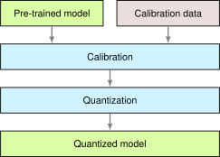](https://mlsysbook.ai/contents/core/optimizations/8d8ca5f84b74881f635a2f9142ea8774f3c82e7e.svg "Figure 18: Post-Training Quantization: Calibration with a representative dataset determines optimal quantization ranges for model weights and activations, minimizing information loss during quantization to create efficient, lower-precision models. This process converts a pre-trained model into a quantized version suitable for deployment on resource-constrained devices.")
Figure 18: **Post-Training Quantization**: Calibration with a representative dataset determines optimal quantization ranges for model weights and activations, minimizing information loss during quantization to create efficient, lower-precision models. This process converts a pre-trained model into a quantized version suitable for deployment on resource-constrained devices.
For example, consider quantizing activations that originally have a floating-point range between –6 and 6 to 8-bit integers. Simply using the full integer range of –128 to 127 for quantization might not be the most effective approach. Instead, calibration involves passing a representative dataset through the model and observing the actual range of the activations. The observed range can then be used to set a more effective quantization range, reducing information loss.
###### Calibration Methods
There are several commonly used calibration methods:
* **Max**: This method uses the maximum absolute value seen during calibration as the clipping range. While simple, it is susceptible to outlier data. For example, in the activation distribution shown in [Figure 19](https://mlsysbook.ai/contents/core/optimizations/optimizations.html#fig-resnet-activations-histogram)
, we see an outlier cluster around 2.1, while the rest of the values are clustered around smaller values. The Max method could lead to an inefficient range if the outliers significantly influence the quantization.
* **Entropy**: This method minimizes information loss between the original floating-point values and the values that could be represented by the quantized format, typically using KL divergence. This is the default calibration method used by TensorRT and works well when trying to preserve the distribution of the original values.
* **Percentile**: This method sets the clipping range to a percentile of the distribution of absolute values seen during calibration. For example, a 99% calibration would clip the top 1% of the largest magnitude values. This method helps avoid the impact of outliers, which are not representative of the general data distribution.
[](https://mlsysbook.ai/contents/core/optimizations/images/png/efficientnumerics_calibrationcopy.png "Figure 19: Activation Distribution: Resnet50 layer activations exhibit a long tail, with a small percentage of values significantly larger than the majority; this distribution impacts quantization range selection, as outlier values can lead to inefficient use of precision if not handled carefully. Source: [@wu2020integer].")
Figure 19: **Activation Distribution**: Resnet50 layer activations exhibit a long tail, with a small percentage of values significantly larger than the majority; this distribution impacts quantization range selection, as outlier values can lead to inefficient use of precision if not handled carefully. Source: ([H. Wu et al. 2020](https://mlsysbook.ai/contents/core/optimizations/optimizations.html#ref-wu2020integer)
).
The quality of calibration directly affects the performance of the quantized model. A poor calibration could lead to a model that suffers from significant accuracy loss, while a well-calibrated model can retain much of its original performance after quantization. There are two types of calibration ranges to consider:
* **Symmetric Calibration**: The clipping range is symmetric around zero, meaning both the positive and negative ranges are equally scaled.
* **Asymmetric Calibration**: The clipping range is not symmetric, which means the positive and negative ranges may have different scaling factors. This can be useful when the data is not centered around zero.
Choosing the right calibration method and range is important for maintaining model accuracy while benefiting from the efficiency gains of reduced precision.
###### Calibration Ranges
A key challenge in post-training quantization is selecting the appropriate calibration range \\(\[\\alpha, \\beta\]\\) to map floating-point values into a lower-precision representation. The choice of this range directly affects the quantization error and, consequently, the accuracy of the quantized model. As illustrated in [Figure 20](https://mlsysbook.ai/contents/core/optimizations/optimizations.html#fig-calibration-ranges)
, there are two primary calibration strategies: symmetric calibration and asymmetric calibration.
[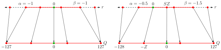](https://mlsysbook.ai/contents/core/optimizations/3c174b55a58765f9e634d15b256323ab81990b40.svg "Figure 20: Calibration Range Selection: Symmetric calibration uses a fixed range around zero, while asymmetric calibration adapts the range to the data distribution, potentially minimizing quantization error and preserving model accuracy. Choosing an appropriate calibration strategy balances precision with the risk of saturation for outlier values.")
Figure 20: **Calibration Range Selection**: Symmetric calibration uses a fixed range around zero, while asymmetric calibration adapts the range to the data distribution, potentially minimizing quantization error and preserving model accuracy. Choosing an appropriate calibration strategy balances precision with the risk of saturation for outlier values.
On the left side of [Figure 20](https://mlsysbook.ai/contents/core/optimizations/optimizations.html#fig-calibration-ranges)
, symmetric calibration is depicted, where the clipping range is centered around zero. The range extends from \\(\\alpha = -1\\) to \\(\\beta = 1\\), mapping these values to the integer range \\(\[-127, 127\]\\). This method ensures that positive and negative values are treated equally, preserving zero-centered distributions. A key advantage of symmetric calibration is its simplified implementation, as the same scale factor is applied to both positive and negative values. However, this approach may not be optimal for datasets where the activation distributions are skewed, leading to poor representation of significant portions of the data.
On the right side, asymmetric calibration is shown, where \\(\\alpha = -0.5\\) and \\(\\beta = 1.5\\). Here, zero is mapped to a shifted quantized value \\(-Z\\), and the range extends asymmetrically. In this case, the quantization scale is adjusted to account for non-zero mean distributions. Asymmetric calibration is particularly useful when activations or weights exhibit skew, ensuring that the full quantized range is effectively utilized. However, it introduces additional computational complexity in determining the optimal offset and scaling factors.
The choice between these calibration strategies depends on the model and dataset characteristics:
* Symmetric calibration is commonly used when weight distributions are centered around zero, which is often the case for well-initialized machine learning models. It simplifies computation and hardware implementation but may not be optimal for all scenarios.
* Asymmetric calibration is useful when the data distribution is skewed, ensuring that the full quantized range is effectively utilized. It can improve accuracy retention but may introduce additional computational complexity in determining the optimal quantization parameters.
Many machine learning frameworks, including TensorRT and PyTorch, support both calibration modes, enabling practitioners to empirically evaluate the best approach. Selecting an appropriate calibration range is important for PTQ, as it directly influences the trade-off between numerical precision and efficiency, ultimately affecting the performance of quantized models.
##### Granularity
After determining the clipping range, the next step in optimizing quantization involves adjusting the granularity of the clipping range to ensure that the model retains as much accuracy as possible. In CNNs, for instance, the input activations of a layer undergo convolution with multiple convolutional filters, each of which may have a unique range of values. The quantization process, therefore, must account for these differences in range across filters to preserve the model’s performance.
As illustrated in [Figure 21](https://mlsysbook.ai/contents/core/optimizations/optimizations.html#fig-quantization-granularity)
, the range for Filter 1 is significantly smaller than that for Filter 3, demonstrating the variation in the magnitude of values across different filters. The precision with which the clipping range \[\\(\\alpha\\), \\(\\beta\\)\] is determined for the weights becomes a important factor in effective quantization. This variability in ranges is a key reason why different quantization strategies, based on granularity, are employed.
[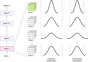](https://mlsysbook.ai/contents/core/optimizations/99152f77f78dd8f02445a6892fc5bf3a4ec98ed0.svg "Figure 21: Quantization Range Variation: Different convolutional filters exhibit unique activation ranges, necessitating per-filter quantization to minimize accuracy loss during quantization. Adjusting the granularity of clipping ranges—as shown by the differing scales for each filter—optimizes the trade-off between model size and performance. Source: [@gholami2021survey].")
Figure 21: **Quantization Range Variation**: Different convolutional filters exhibit unique activation ranges, necessitating per-filter quantization to minimize accuracy loss during quantization. Adjusting the granularity of clipping ranges—as shown by the differing scales for each filter—optimizes the trade-off between model size and performance. Source: ([Gholami et al. 2021](https://mlsysbook.ai/contents/core/optimizations/optimizations.html#ref-gholami2021survey)
).
Several methods are commonly used to determine the granularity of quantization, each with its own trade-offs in terms of accuracy, efficiency, and computational cost.
###### Layerwise Quantization
In this approach, the clipping range is determined by considering all weights in the convolutional filters of a layer. The same clipping range is applied to all filters within the layer. While this method is simple to implement, it often leads to suboptimal accuracy due to the wide range of values across different filters. For example, if one convolutional kernel has a narrower range of values than another in the same layer, the quantization resolution of the narrower range may be compromised, resulting in a loss of information.
###### Groupwise Quantization
Groupwise quantization divides the convolutional filters into groups and calculates a shared clipping range for each group. This method can be beneficial when the distribution of values within a layer is highly variable. For example, the Q-BERT model ([Shen et al. 2019](https://mlsysbook.ai/contents/core/optimizations/optimizations.html#ref-sheng2019qbert)
) applied this technique when quantizing Transformer models ([Chen et al. 2018](https://mlsysbook.ai/contents/core/optimizations/optimizations.html#ref-vaswani2017attention)
), particularly for the fully-connected attention layers. While groupwise quantization offers better accuracy than layerwise quantization, it incurs additional computational cost due to the need to account for multiple scaling factors.
Shen, Sheng, Zhen Dong, Jiayu Ye, Linjian Ma, Zhewei Yao, Amir Gholami, Michael W. Mahoney, and Kurt Keutzer. 2019. “Q-BERT: Hessian Based Ultra Low Precision Quantization of BERT.” _Proceedings of the AAAI Conference on Artificial Intelligence_ 34 (05): 8815–21. [https://doi.org/10.1609/aaai.v34i05.6409](https://doi.org/10.1609/aaai.v34i05.6409)
.
Chen, Mia Xu, Orhan Firat, Ankur Bapna, Melvin Johnson, Wolfgang Macherey, George Foster, Llion Jones, et al. 2018. “The Best of Both Worlds: Combining Recent Advances in Neural Machine Translation.” In _Proceedings of the 56th Annual Meeting of the Association for Computational Linguistics (Volume 1: Long Papers)_, 30:5998–6008. Association for Computational Linguistics. [https://doi.org/10.18653/v1/p18-1008](https://doi.org/10.18653/v1/p18-1008)
.
###### Channelwise Quantization
Channelwise quantization assigns a dedicated clipping range and scaling factor to each convolutional filter. This approach ensures a higher resolution in quantization, as each channel is quantized independently. Channelwise quantization is widely used in practice, as it often yields better accuracy compared to the previous methods. By allowing each filter to have its own clipping range, this method ensures that the quantization process is tailored to the specific characteristics of each filter.
###### Sub-channelwise Quantization
Sub-channelwise quantization subdivides each convolutional filter into smaller groups, each with its own clipping range. Although it provides very fine-grained control over quantization, it introduces significant computational overhead as multiple scaling factors must be managed for each group within a filter. As a result, sub-channelwise quantization is generally only used in scenarios where maximum precision is required, despite the increased computational cost.
Among these methods, channelwise quantization is the current standard for quantizing convolutional filters. It strikes a balance between the accuracy gains from finer granularity and the computational efficiency needed for practical deployment. Adjusting the clipping range for each individual kernel provides significant improvements in model accuracy with minimal overhead, making it the most widely adopted approach in machine learning applications.
##### Weights vs. Activations
Weight Quantization involves converting the continuous, high-precision weights of a model into lower-precision values, such as converting 32-bit floating-point (Float32) weights to 8-bit integer (INT8) weights. As illustrated in [Figure 22](https://mlsysbook.ai/contents/core/optimizations/optimizations.html#fig-weight-activations-quantization)
, weight quantization occurs in the second step (red squares) during the multiplication of inputs. This process significantly reduces the model size, decreasing both the memory required to store the model and the computational resources needed for inference. For example, a weight matrix in a neural network layer with Float32 weights like \\(\[0.215, -1.432, 0.902,\\ldots\]\\) might be mapped to INT8 values such as \\(\[27, -183, 115, \\ldots\]\\), leading to a significant reduction in memory usage.
[](https://mlsysbook.ai/contents/core/optimizations/ba3ce40aa09ea580e4583ff539ba290a72f03357.svg "Figure 22: Quantization and Weight Precision: Reducing weight and activation precision from float32 to INT8 significantly lowers model size and computational cost during inference by representing values with fewer bits, though it may introduce a trade-off with model accuracy. This process alters the numerical representation of model parameters and intermediate results, impacting both memory usage and processing speed. Source: HarvardX.")
Figure 22: **Quantization and Weight Precision**: Reducing weight and activation precision from float32 to INT8 significantly lowers model size and computational cost during inference by representing values with fewer bits, though it may introduce a trade-off with model accuracy. This process alters the numerical representation of model parameters and intermediate results, impacting both memory usage and processing speed. Source: HarvardX.
Activation Quantization refers to the process of quantizing the activation values, or outputs of the layers, during model inference. This quantization can reduce the computational resources required during inference, particularly when targeting hardware optimized for integer arithmetic. It introduces challenges related to maintaining model accuracy, as the precision of intermediate computations is reduced. For instance, in a CNN, the activation maps (or feature maps) produced by convolutional layers, originally represented in Float32, may be quantized to INT8 during inference. This can significantly accelerate computation on hardware capable of efficiently processing lower-precision integers.
Recent advancements have explored Activation-aware Weight Quantization (AWQ) for the compression and acceleration of large language models (LLMs). This approach focuses on protecting only a small fraction of the most salient weights, approximately 1%, by observing the activations rather than the weights themselves. This method has been shown to improve model efficiency while preserving accuracy, as discussed in ([Ji Lin et al. 2023](https://mlsysbook.ai/contents/core/optimizations/optimizations.html#ref-lin2023awq)
).
Lin, Ji, Jiaming Tang, Haotian Tang, Shang Yang, Wei-Ming Chen, Wei-Chen Wang, Guangxuan Xiao, Xingyu Dang, Chuang Gan, and Song Han. 2023. “AWQ: Activation-Aware Weight Quantization for LLM Compression and Acceleration.” _arXiv Preprint arXiv:2306.00978_ abs/2306.00978 (June). [http://arxiv.org/abs/2306.00978v5](http://arxiv.org/abs/2306.00978v5)
.
##### Static vs. Dynamic Quantization
After determining the type and granularity of the clipping range, practitioners must decide when the clipping ranges are calculated in their quantization algorithms. Two primary approaches exist for quantizing activations: static quantization and dynamic quantization.
Static Quantization is the more commonly used approach. In static quantization, the clipping range is pre-calculated and remains fixed during inference. This method does not introduce any additional computational overhead during runtime, which makes it efficient in terms of computational resources. However, the fixed range can lead to lower accuracy compared to dynamic quantization. A typical implementation of static quantization involves running a series of calibration inputs to compute the typical range of activations ([Jacob et al. 2018a](https://mlsysbook.ai/contents/core/optimizations/optimizations.html#ref-jacob2018quantization)
; [Yao et al. 2021](https://mlsysbook.ai/contents/core/optimizations/optimizations.html#ref-yao2021hawq)
).
Yao, Zhewei, Amir Gholami, Sheng Shen, Kurt Keutzer, and Michael W. Mahoney. 2021. “HAWQ-V3: Dyadic Neural Network Quantization.” In _Proceedings of the 38th International Conference on Machine Learning (ICML)_, 11875–86. PMLR.
In contrast, Dynamic Quantization dynamically calculates the range for each activation map during runtime. This approach allows the quantization process to adjust in real time based on the input, potentially yielding higher accuracy since the range is specifically calculated for each input activation. However, dynamic quantization incurs higher computational overhead because the range must be recalculated at each step. Although this often results in higher accuracy, the real-time computations can be expensive, particularly when deployed at scale.
The following table, [Table 8](https://mlsysbook.ai/contents/core/optimizations/optimizations.html#tbl-quantization_methods)
, summarizes the characteristics of post-training quantization, quantization-aware training, and dynamic quantization, providing an overview of their respective strengths, limitations, and trade-offs. These methods are widely deployed across machine learning systems of varying scales, and understanding their pros and cons is important for selecting the appropriate approach for a given application.
Table 8: **Quantization Trade-Offs**: Post-training quantization, quantization-aware training, and dynamic quantization represent distinct approaches to model compression, each balancing accuracy, computational cost, and implementation complexity for machine learning systems. Understanding these trade-offs is important for selecting the optimal quantization strategy based on application requirements and resource constraints.
| | | | |
| --- | --- | --- | --- |
| **Pros** | | | |
| **Simplicity** | ✓ | ✗ | ✗ |
| **Accuracy Preservation** | ✗ | ✓ | ✓ |
| **Adaptability** | ✗ | ✗ | ✓ |
| **Optimized Performance** | ✗ | ✓ | Potentially |
| **Cons** | | | |
| **Accuracy Degradation** | ✓ | ✗ | Potentially |
| **Computational Overhead** | ✗ | ✓ | ✓ |
| **Implementation Complexity** | ✗ | ✓ | ✓ |
| **Tradeoffs** | | | |
| **Speed vs. Accuracy** | ✓ | ✗ | ✗ |
| **Accuracy vs. Cost** | ✗ | ✓ | ✗ |
| **Adaptability vs. Overhead** | ✗ | ✗ | ✓ |
##### PTQ Advantages
One of the key advantages of PTQ is its low computational cost, as it does not require retraining the model. This makes it an attractive option for the rapid deployment of trained models, particularly when retraining is computationally expensive or infeasible. Since PTQ only modifies the numerical representation of weights and activations, the underlying model architecture remains unchanged, allowing it to be applied to a wide range of pre-trained models without modification.
PTQ also provides significant memory and storage savings by reducing the bit-width of model parameters. For instance, converting a model from FP32 to INT8 results in a \\(4\\times\\) reduction in storage size, making it feasible to deploy larger models on resource-constrained devices such as mobile phones, edge AI hardware, and embedded systems. These reductions in memory footprint also lead to lower bandwidth requirements when transferring models across networked systems.
In terms of computational efficiency, PTQ allows inference to be performed using integer arithmetic, which is inherently faster than floating-point operations on many hardware platforms. AI accelerators such as TPUs and Neural Processing Units (NPUs) are optimized for lower-precision computations, enabling higher throughput and reduced power consumption when executing quantized models. This makes PTQ particularly useful for applications requiring real-time inference, such as object detection in autonomous systems or speech recognition on mobile devices.
##### PTQ Challenges and Limitations
Despite its advantages, PTQ introduces quantization errors due to rounding effects when mapping floating-point values to discrete lower-precision representations. While some models remain robust to these changes, others may experience notable accuracy degradation, especially in tasks that rely on small numerical differences.
The extent of accuracy loss depends on both the model architecture and the task domain. CNNs for image classification are generally tolerant to PTQ, often maintaining near-original accuracy even with aggressive INT8 quantization. Transformer-based models used in NLP and speech recognition tend to be more sensitive, as these architectures rely on the precision of numerical relationships in attention mechanisms.
To mitigate accuracy loss, calibration techniques such as KL divergence-based scaling or per-channel quantization are commonly applied to fine-tune the scaling factor and minimize information loss. Some frameworks, including TensorFlow Lite and PyTorch, provide automated quantization tools with built-in calibration methods to improve accuracy retention.
Another limitation of PTQ is that not all hardware supports efficient integer arithmetic. While GPUs, TPUs, and specialized edge AI chips often include dedicated support for INT8 inference, general-purpose CPUs may lack the optimized instructions for low-precision execution, resulting in suboptimal performance improvements.
PTQ is not always suitable for training purposes. Since PTQ applies quantization after training, models that require further fine-tuning or adaptation may benefit more from alternative approaches, such as quantization-aware training (discussed next), to ensure that precision constraints are adequately considered during the learning process.
Post-training quantization remains one of the most practical and widely used techniques for improving inference efficiency. It provides significant memory and computational savings with minimal overhead, making it an ideal choice for deploying machine learning models in resource-constrained environments. However, the success of PTQ depends on model architecture, task sensitivity, and hardware compatibility. In scenarios where accuracy degradation is unacceptable, alternative quantization strategies, such as quantization-aware training, may be required.
Post-training quantization provides the foundation for more advanced quantization methods. The core concepts—quantization workflows, numerical format trade-offs, and calibration methods—remain essential throughout all precision optimization techniques. For rapid deployment scenarios with production deadlines under two weeks and acceptable accuracy loss of 1-2%, PTQ with min-max calibration often provides a complete solution. Production systems requiring less than 1% accuracy loss should consider Quantization-Aware Training, which recovers accuracy through fine-tuning with quantization simulation at the cost of 20-50% additional training time. Extreme constraints like sub-1MB models or sub-10mW power budgets may require INT4 or binary quantization, accepting 5-20% accuracy degradation that necessitates architectural changes.
#### Quantization-Aware Training
QAT integrates quantization constraints directly into the training process, simulating low-precision arithmetic during forward passes to allow the model to adapt to quantization effects ([Jacob et al. 2018a](https://mlsysbook.ai/contents/core/optimizations/optimizations.html#ref-jacob2018quantization)
). This approach proves particularly important for models requiring fine-grained numerical precision, such as transformers used in NLP and speech recognition systems ([Nagel et al. 2021b](https://mlsysbook.ai/contents/core/optimizations/optimizations.html#ref-nagel2021whitepaper)
). [Figure 23](https://mlsysbook.ai/contents/core/optimizations/optimizations.html#fig-qat)
illustrates the QAT process: quantization is applied to a pre-trained model, followed by fine-tuning to adapt weights to low-precision constraints.
———. 2018a. “Quantization and Training of Neural Networks for Efficient Integer-Arithmetic-Only Inference.” In _2018 IEEE/CVF Conference on Computer Vision and Pattern Recognition_, 2704–13. IEEE. [https://doi.org/10.1109/cvpr.2018.00286](https://doi.org/10.1109/cvpr.2018.00286)
.
———. 2021b. “A White Paper on Neural Network Quantization.” _arXiv Preprint arXiv:2106.08295_, June. [http://arxiv.org/abs/2106.08295v1](http://arxiv.org/abs/2106.08295v1)
.
[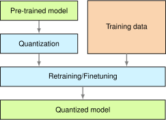](https://mlsysbook.ai/contents/core/optimizations/8b5682dff49bc4715df9b14d4a3e6ed9c70c325a.svg "Figure 23: Quantization-Aware Training: Retraining a pre-trained model with simulated low-precision arithmetic adapts weights to mitigate accuracy loss during deployment with reduced numerical precision, enabling efficient inference on resource-constrained devices. This process refines the model to become robust to the effects of quantization, maintaining performance despite lower precision representations.")
Figure 23: **Quantization-Aware Training**: Retraining a pre-trained model with simulated low-precision arithmetic adapts weights to mitigate accuracy loss during deployment with reduced numerical precision, enabling efficient inference on resource-constrained devices. This process refines the model to become robust to the effects of quantization, maintaining performance despite lower precision representations.
In many cases, QAT can also build off PTQ (discussed in detail in the previous section), as shown in [Figure 24](https://mlsysbook.ai/contents/core/optimizations/optimizations.html#fig-ptq-qat)
. Instead of starting from a full-precision model, PTQ is first applied to produce an initial quantized model using calibration data. This quantized model then serves as the starting point for QAT, where additional fine-tuning with training data helps the model better adapt to low-precision constraints. This hybrid approach combines PTQ’s efficiency with QAT’s accuracy preservation, reducing the degradation typically associated with post-training approaches alone.
[](https://mlsysbook.ai/contents/core/optimizations/346c0a0d25f22b314c8a749395cd79e069a3c62c.svg "Figure 24: Hybrid Quantization Approach: Post-training quantization (PTQ) generates an initial quantized model that serves as a warm start for quantization-aware training (QAT), accelerating convergence and mitigating accuracy loss compared to quantizing a randomly initialized network. This two-stage process leverages the efficiency of PTQ while refining the model with training data to optimize performance under low-precision constraints.")
Figure 24: **Hybrid Quantization Approach**: Post-training quantization (PTQ) generates an initial quantized model that serves as a warm start for quantization-aware training (QAT), accelerating convergence and mitigating accuracy loss compared to quantizing a randomly initialized network. This two-stage process leverages the efficiency of PTQ while refining the model with training data to optimize performance under low-precision constraints.
##### Training Mathematics
During forward propagation, weights and activations are quantized and dequantized to mimic reduced precision. This process is typically represented as: \\\[ q = \\text{round} \\left(\\frac{x}{s} \\right) \\times s \\\] where \\(q\\) represents the simulated quantized value, \\(x\\) denotes the full-precision weight or activation, and \\(s\\) is the scaling factor mapping floating-point values to lower-precision integers.
Although the forward pass utilizes quantized values, gradient calculations during backpropagation remain in full precision. This is achieved using the Straight-Through Estimator (STE)[32](https://mlsysbook.ai/contents/core/optimizations/optimizations.html#fn32)
, which approximates the gradient of the quantized function by treating the rounding operation as if it had a derivative of one. This approach prevents the gradient from being obstructed due to the non-differentiable nature of the quantization operation, thereby allowing effective model training ([Y. Bengio, Léonard, and Courville 2013a](https://mlsysbook.ai/contents/core/optimizations/optimizations.html#ref-bengio2013estimating)
).
32 **Straight-Through Estimator (STE)**: Gradient approximation technique for non-differentiable functions, introduced by Bengio et al. ([Y. Bengio, Léonard, and Courville 2013a](https://mlsysbook.ai/contents/core/optimizations/optimizations.html#ref-bengio2013estimating)
). Sets gradient of step function to 1 everywhere, enabling backpropagation through quantization layers. Crucial for training binarized neural networks and quantization-aware training, despite theoretical limitations around zero.
———. 2013a. “Estimating or Propagating Gradients Through Stochastic Neurons for Conditional Computation.” _arXiv Preprint arXiv:1308.3432_, August. [http://arxiv.org/abs/1308.3432v1](http://arxiv.org/abs/1308.3432v1)
.
Krishnamoorthi, Raghuraman. 2018. “Quantizing Deep Convolutional Networks for Efficient Inference: A Whitepaper.” _arXiv Preprint arXiv:1806.08342_ abs/1806.08342 (June). [http://arxiv.org/abs/1806.08342v1](http://arxiv.org/abs/1806.08342v1)
.
Integrating quantization effects during training enables the model to learn an optimal distribution of weights and activations that minimizes the impact of numerical precision loss. The resulting model, when deployed using true low-precision arithmetic (e.g., INT8 inference), maintains significantly higher accuracy than one that is quantized post hoc ([Krishnamoorthi 2018](https://mlsysbook.ai/contents/core/optimizations/optimizations.html#ref-krishnamoorthi2018quantizing)
).
##### QAT Advantages
A primary advantage of QAT[33](https://mlsysbook.ai/contents/core/optimizations/optimizations.html#fn33)
is its ability to maintain model accuracy, even under low-precision inference conditions. Incorporating quantization during training helps the model to compensate for precision loss, reducing the impact of rounding errors and numerical instability. This is important for quantization-sensitive models commonly used in NLP, speech recognition, and high-resolution computer vision ([Gholami et al. 2021](https://mlsysbook.ai/contents/core/optimizations/optimizations.html#ref-gholami2021survey)
).
33 **Quantization-Aware Training**: QAT enables INT8 inference with minimal accuracy loss - ResNet-50 maintains 76.1% vs. 76.2% FP32 ImageNet accuracy, while MobileNetV2 achieves 71.8% vs. 72.0%. BERT-Base INT8 retains 99.1% of FP32 performance on GLUE, compared to 96.8% with post-training quantization alone.
Gholami, Amir, Sehoon Kim, Zhen Dong, Zhewei Yao, Michael W. Mahoney, and Kurt Keutzer. 2021. “A Survey of Quantization Methods for Efficient Neural Network Inference.” _arXiv Preprint arXiv:2103.13630_ abs/2103.13630 (March). [http://arxiv.org/abs/2103.13630v3](http://arxiv.org/abs/2103.13630v3)
.
Wu, Hao, Patrick Judd, Xiaojie Zhang, Mikhail Isaev, and Paulius Micikevicius. 2020. “Integer Quantization for Deep Learning Inference: Principles and Empirical Evaluation.” _arXiv Preprint arXiv:2004.09602_ abs/2004.09602 (April). [http://arxiv.org/abs/2004.09602v1](http://arxiv.org/abs/2004.09602v1)
.
Another major benefit is that QAT permits low-precision inference on hardware accelerators without significant accuracy degradation. AI processors such as TPUs, NPUs, and specialized edge devices include dedicated hardware for integer operations, permitting INT8 models to run much faster and with lower energy consumption compared to FP32 models. Training with quantization effects in mind ensures that the final model can fully leverage these hardware optimizations ([H. Wu et al. 2020](https://mlsysbook.ai/contents/core/optimizations/optimizations.html#ref-wu2020integer)
).
##### QAT Challenges and Trade-offs
Despite its benefits, QAT introduces additional computational overhead during training. Simulated quantization at every forward pass slows down training relative to full-precision methods. The process adds complexity to the training schedule, making QAT less practical for very large-scale models where the additional training time might be prohibitive.
QAT introduces extra hyperparameters and design considerations, such as choosing appropriate quantization schemes and scaling factors. Unlike PTQ, which applies quantization after training, QAT requires careful tuning of the training dynamics to ensure that the model suitably adapts to low-precision constraints ([Gong et al. 2019](https://mlsysbook.ai/contents/core/optimizations/optimizations.html#ref-choukroun2019low)
).
Gong, Ruihao, Xianglong Liu, Shenghu Jiang, Tianxiang Li, Peng Hu, Jiazhen Lin, Fengwei Yu, and Junjie Yan. 2019. “Differentiable Soft Quantization: Bridging Full-Precision and Low-Bit Neural Networks.” _arXiv Preprint arXiv:1908.05033_, August. [http://arxiv.org/abs/1908.05033v1](http://arxiv.org/abs/1908.05033v1)
.
[Table 9](https://mlsysbook.ai/contents/core/optimizations/optimizations.html#tbl-qat)
summarizes the key trade-offs of QAT compared to PTQ:
Table 9: **Quantization Trade-Offs**: Quantization-aware training (QAT) minimizes accuracy loss from reduced numerical precision by incorporating quantization into the training process, while post-training quantization (PTQ) offers faster deployment but may require calibration to mitigate accuracy degradation. QAT’s retraining requirement increases training complexity compared to the simplicity of applying PTQ to a pre-trained model.
| | | |
| --- | --- | --- |
| **Accuracy Retention** | Minimizes accuracy loss from quantization | May suffer from accuracy degradation |
| **Inference Efficiency** | Optimized for low-precision hardware (e.g., INT8 on TPUs) | Optimized but may require calibration |
| **Training Complexity** | Requires retraining with quantization constraints | No retraining required |
| **Training Time** | Slower due to simulated quantization in forward pass | Faster, as quantization is applied post hoc |
| **Deployment Readiness** | Best for models sensitive to quantization errors | Fastest way to optimize models for inference |
Integrating quantization into the training process preserves model accuracy more effectively than post-training quantization, although it requires additional training resources and time.
##### PTQ vs. QAT
The choice between PTQ and QAT depends on trade-offs between accuracy, computational cost, and deployment constraints. PTQ provides computationally inexpensive optimization requiring only post-training conversion, making it ideal for rapid deployment. However, effectiveness varies by architecture—CNNs tolerate PTQ well while NLP and speech models may experience degradation due to reliance on precise numerical representations.
QAT proves necessary when high accuracy retention is critical. Integrating quantization effects during training allows models to adapt to lower-precision arithmetic, reducing quantization errors ([Jacob et al. 2018b](https://mlsysbook.ai/contents/core/optimizations/optimizations.html#ref-Jacob2018)
). While achieving higher low-precision accuracy, QAT requires additional training time and computational resources. In practice, a hybrid approach starting with PTQ and selectively applying QAT for accuracy-critical models provides optimal balance between efficiency and performance.
### Extreme Quantization
Beyond INT8 and INT4 quantization, extreme quantization techniques use 1-bit (binarization) or 2-bit (ternarization) representations to achieve dramatic reductions in memory usage and computational requirements ([Courbariaux, Bengio, and David 2016](https://mlsysbook.ai/contents/core/optimizations/optimizations.html#ref-Courbariaux2016)
). Binarization constrains weights and activations to two values (typically -1 and +1, or 0 and 1), drastically reducing model size and accelerating inference on specialized hardware like binary neural networks ([Rastegari et al. 2016](https://mlsysbook.ai/contents/core/optimizations/optimizations.html#ref-Rastegari2016)
). However, this constraint severely limits model expressiveness, often degrading accuracy on tasks requiring high precision such as image recognition or natural language processing ([Hubara et al. 2018](https://mlsysbook.ai/contents/core/optimizations/optimizations.html#ref-Hubara2018)
).
Courbariaux, Matthieu, Yoshua Bengio, and Jean-Pierre David. 2016. “BinaryConnect: Training Deep Neural Networks with Binary Weights During Propagations.” _Advances in Neural Information Processing Systems (NeurIPS)_ 28: 3123–31.
Rastegari, Mohammad, Vicente Ordonez, Joseph Redmon, and Ali Farhadi. 2016. “XNOR-Net: ImageNet Classification Using Binary Convolutional Neural Networks.” In _Computer Vision – ECCV 2016_, 525–42. Springer International Publishing. [https://doi.org/10.1007/978-3-319-46493-0\\\_32](https://doi.org/10.1007/978-3-319-46493-0/_32)
.
Hubara, Itay, Matthieu Courbariaux, Daniel Soudry, Ran El-Yaniv, and Yoshua Bengio. 2018. “Quantized Neural Networks: Training Neural Networks with Low Precision Weights and Activations.” _Journal of Machine Learning Research (JMLR)_ 18: 1–30.
Zhu, Chenzhuo, Song Han, Huizi Mao, and William J. Dally. 2017. “Trained Ternary Quantization.” _International Conference on Learning Representations (ICLR)_.
Bengio, Yoshua, Nicholas Léonard, and Aaron Courville. 2013b. “Estimating or Propagating Gradients Through Stochastic Neurons for Conditional Computation.” _arXiv Preprint_, August. [http://arxiv.org/abs/1308.3432v1](http://arxiv.org/abs/1308.3432v1)
.
Choi, Jungwook, Zhuo Wang, Swagath Venkataramani, Pierce I-Jen Chuang, Vijayalakshmi Srinivasan, and Kailash Gopalakrishnan. 2018. “PACT: Parameterized Clipping Activation for Quantized Neural Networks.” _arXiv Preprint_, May. [http://arxiv.org/abs/1805.06085v2](http://arxiv.org/abs/1805.06085v2)
.
Ternarization extends binarization by allowing three values (-1, 0, +1), providing additional flexibility that slightly improves accuracy over pure binarization ([Zhu et al. 2017](https://mlsysbook.ai/contents/core/optimizations/optimizations.html#ref-Zhu2017)
). The zero value enables greater sparsity while maintaining more representational power. Both techniques require gradient approximation methods like Straight-Through Estimator (STE) to handle non-differentiable quantization operations during training ([Y. Bengio, Léonard, and Courville 2013b](https://mlsysbook.ai/contents/core/optimizations/optimizations.html#ref-Bengio2013)
), with QAT integration helping mitigate accuracy loss ([Choi et al. 2018](https://mlsysbook.ai/contents/core/optimizations/optimizations.html#ref-Choi2019)
).
##### Challenges and Limitations
Despite enabling ultra-low-power machine learning for embedded systems and mobile devices, binarization and ternarization face significant challenges. Performance maintenance proves difficult with such drastic quantization, requiring specialized hardware capable of efficiently handling binary or ternary operations ([Umuroglu et al. 2017](https://mlsysbook.ai/contents/core/optimizations/optimizations.html#ref-Umuroglu2017)
). Traditional processors lack optimization for these computations, necessitating custom hardware accelerators.
Umuroglu, Yaman, Nicholas J. Fraser, Giulio Gambardella, Michaela Blott, Philip Leong, Magnus Jahre, and Kees Vissers. 2017. “FINN: A Framework for Fast, Scalable Binarized Neural Network Inference.” In _Proceedings of the 2017 ACM/SIGDA International Symposium on Field-Programmable Gate Arrays_, 65–74. ACM. [https://doi.org/10.1145/3020078.3021744](https://doi.org/10.1145/3020078.3021744)
.
Jacob, Benoit, Skirmantas Kligys, Bo Chen, Menglong Zhu, Matthew Tang, Andrew Howard, Hartwig Adam, and Dmitry Kalenichenko. 2018b. “Quantization and Training of Neural Networks for Efficient Integer-Arithmetic-Only Inference.” In _2018 IEEE/CVF Conference on Computer Vision and Pattern Recognition_, 2704–13. IEEE. [https://doi.org/10.1109/cvpr.2018.00286](https://doi.org/10.1109/cvpr.2018.00286)
.
Accuracy loss remains a critical concern. These methods suit tasks where high precision is not critical or where QAT can compensate for precision constraints. Despite challenges, the ability to drastically reduce model size while maintaining acceptable accuracy makes them attractive for edge AI and resource-constrained environments ([Jacob et al. 2018b](https://mlsysbook.ai/contents/core/optimizations/optimizations.html#ref-Jacob2018)
). Future advances in specialized hardware and training techniques will likely enhance their role in efficient, scalable AI.
### Multi-Technique Optimization Strategies
Having explored quantization techniques (PTQ, QAT, binarization, and ternarization), pruning methods, and knowledge distillation, we now examine how these complementary approaches can be systematically combined to achieve superior optimization results. Rather than applying techniques in isolation, integrated strategies leverage the synergies between different optimization dimensions to maximize efficiency gains while preserving model accuracy.
Each optimization technique addresses distinct aspects of model efficiency: quantization reduces numerical precision, pruning eliminates redundant parameters, knowledge distillation transfers capabilities to compact architectures, and NAS optimizes structural design. These techniques exhibit complementary characteristics that enable powerful combinations.
Pruning and quantization create synergistic effects because pruning reduces parameter count while quantization reduces precision, creating multiplicative compression effects. Applying pruning first reduces the parameter set, making subsequent quantization more effective and reducing the search space for optimal quantization strategies. This sequential approach can achieve compression ratios exceeding either technique alone.
Knowledge distillation integrates effectively with quantization by mitigating accuracy loss from aggressive quantization. This approach trains student models to match teacher behavior rather than just minimizing task loss, proving particularly effective for extreme quantization scenarios where direct quantization would cause unacceptable accuracy degradation.
Neural architecture search enables co-design approaches that optimize model structures specifically for quantization constraints, identifying architectures that maintain accuracy under low-precision operations. This co-design approach produces models inherently suited for subsequent optimization, improving the effectiveness of both quantization and pruning techniques.
As shown in [Figure 25](https://mlsysbook.ai/contents/core/optimizations/optimizations.html#fig-compression-methods)
, different compression strategies such as pruning, quantization, and singular value decomposition (SVD) exhibit varying trade-offs between model size and accuracy loss. While pruning combined with quantization (red circles) achieves high compression ratios with minimal accuracy loss, quantization alone (yellow squares) also provides a reasonable balance. In contrast, SVD (green diamonds) requires a larger model size to maintain accuracy, illustrating how different techniques can impact compression effectiveness.
[](https://mlsysbook.ai/contents/core/optimizations/9933162e32a3b8b5e0c07c0485a8ece150a8f4ee.svg "Figure 25: Compression Trade-Offs: Combining pruning and quantization achieves superior compression ratios with minimal accuracy loss compared to quantization or singular value decomposition (SVD) alone, demonstrating the impact of different numerical precision optimization techniques on model size and performance. Architectural and numerical optimizations can complement each other to efficiently deploy machine learning models via this figure. Source: [@han2015deep].")
Figure 25: **Compression Trade-Offs**: Combining pruning and quantization achieves superior compression ratios with minimal accuracy loss compared to quantization or singular value decomposition (SVD) alone, demonstrating the impact of different numerical precision optimization techniques on model size and performance. Architectural and numerical optimizations can complement each other to efficiently deploy machine learning models via this figure. Source: ([Han, Mao, and Dally 2015](https://mlsysbook.ai/contents/core/optimizations/optimizations.html#ref-han2015deep)
).
Han, Song, Huizi Mao, and William J. Dally. 2015. “Deep Compression: Compressing Deep Neural Networks with Pruning, Trained Quantization and Huffman Coding.” _arXiv Preprint arXiv:1510.00149_, October. [http://arxiv.org/abs/1510.00149v5](http://arxiv.org/abs/1510.00149v5)
.
Quantization differs from pruning, knowledge distillation, and NAS in that it specifically focuses on reducing the numerical precision of weights and activations. While quantization alone can provide significant computational benefits, its effectiveness can be amplified when combined with the complementary techniques of pruning, distillation, and NAS. These methods, each targeting a different aspect of model efficiency, work together to create more compact, faster, and energy-efficient models, enabling better performance in constrained environments.
Our optimization journey continues. We pruned BERT-Base from 440MB to 110MB through structured pruning and knowledge distillation, then quantized it to INT8, reducing the model to 28MB with inference latency dropping from 120ms to 45ms on mobile hardware. These optimizations transformed an unusable model into one approaching deployment viability. Yet profiling reveals a puzzling inefficiency: theoretical FLOP count suggests inference should complete in 25ms, yet actual execution takes 45ms. Where does the remaining 20ms disappear?
Detailed profiling exposes the answer. While quantization reduced precision, the model still computes zeros unnecessarily. Structured pruning removed entire attention heads, but the remaining sparse weight matrices are stored in dense format, wasting both memory bandwidth and computation on zero-valued elements. Layer normalization operations run sequentially despite their inherent parallelism. The model processes all tokens identically, even though simple inputs could exit early from shallow layers. The GPU spends 40% of execution time idle, waiting for memory transfers rather than executing operations.
These observations reveal why model representation and numerical precision optimizations, while necessary, are insufficient. Representation techniques determine what computations are performed. Precision techniques determine how individual operations execute. But neither addresses how computations are organized and scheduled to maximize hardware utilization. This is the domain of architectural efficiency optimization, the third dimension of our framework.
Architectural efficiency techniques transform the execution pattern itself. Exploiting sparsity through specialized kernels eliminates computation on pruned weights. Operator fusion combines sequential operations (layer norm, attention, feedforward) into single GPU kernels, reducing memory traffic by 40%. Dynamic computation enables simple inputs to exit after 6 layers rather than processing all 12 layers. Hardware-aware scheduling parallelizes operations to maintain high GPU utilization. Applying these techniques to our optimized BERT model reduces inference from 45ms to 22ms, finally achieving the 25ms theoretical target and making deployment truly viable.
This progression illustrates why all three optimization dimensions must work in concert. Model representation provides structural efficiency (fewer parameters). Numerical precision provides computational efficiency (lower precision arithmetic). Architectural efficiency provides execution efficiency (optimized scheduling and hardware utilization). The compound effect, 440MB/120ms → 28MB/22ms (16x memory reduction, 5.5x latency improvement), emerges only when all dimensions are addressed systematically.
**Self-Check: Question 1.7**
1. Which of the following precision formats offers the best balance between computational speed and accuracy for training on AI accelerators?
1. BFloat16
2. FP16
3. INT8
4. FP32
2. Explain the trade-offs involved in using INT8 precision for inference in machine learning models.
3. The process of reducing numerical precision to improve computational efficiency is known as \_\_\_\_. This technique is essential for optimizing machine learning models for deployment in resource-constrained environments.
4. True or False: Reducing precision from FP32 to FP16 always leads to a proportional decrease in power consumption.
5. Order the following precision formats by their typical storage reduction compared to FP32: (1) FP16, (2) INT8, (3) BFloat16.
[See Answers →](https://mlsysbook.ai/contents/core/optimizations/optimizations.html#quiz-answer-sec-model-optimizations-quantization-precision-optimization-e90a)
Architectural Efficiency Techniques
-----------------------------------
Architectural efficiency optimization ensures that computations execute efficiently on target hardware by aligning model operations with processor capabilities and memory hierarchies. Unlike representation optimization (which determines what computations to perform) and precision optimization (which determines numerical fidelity), architectural efficiency addresses how operations are scheduled, how memory is accessed, and how workloads adapt to input characteristics and hardware constraints.
This optimization dimension proves particularly important for resource-constrained scenarios (**[Chapter 14: On-Device Learning](https://mlsysbook.ai/contents/core/ondevice_learning/ondevice_learning.html#sec-ondevice-learning)
**), where theoretical FLOP reductions from pruning and quantization may not translate to actual speedups without architectural modifications. Sparse weight matrices stored in dense format waste memory bandwidth. Sequential operations that could execute in parallel underutilize GPU cores. Fixed computation graphs process simple and complex inputs identically, wasting resources on unnecessary work.
This section examines four complementary approaches to architectural efficiency: hardware-aware design principles that proactively integrate deployment constraints during model development, sparsity exploitation techniques that accelerate computation on pruned models, dynamic computation strategies that adapt workload to input complexity, and operator fusion methods that reduce memory traffic by combining operations. These techniques transform algorithmic optimizations into realized performance gains.
### Hardware-Aware Design
Hardware-aware design incorporates target platform constraints—memory bandwidth, processing power, parallelism capabilities, and energy budgets—directly into model architecture decisions. Rather than optimizing models after training, this approach ensures computational patterns, memory access, and operation types match hardware capabilities from the outset, maximizing efficiency across diverse deployment platforms.
#### Efficient Design Principles
Designing machine learning models for hardware efficiency requires structuring architectures to account for computational cost, memory usage, inference latency, and power consumption, all while maintaining strong predictive performance. Unlike post-training optimizations, which attempt to recover efficiency after training, hardware-aware model design proactively integrates hardware considerations from the outset. This ensures that models are computationally efficient and deployable across diverse hardware environments with minimal adaptation.
Central to this proactive approach, a key aspect of hardware-aware design is using the strengths of specific hardware platforms (e.g., GPUs, TPUs, mobile or edge devices) to maximize parallelism, optimize memory hierarchies, and minimize latency through hardware-optimized operations. As summarized in [Table 10](https://mlsysbook.ai/contents/core/optimizations/optimizations.html#tbl-hardware-efficient-design)
, hardware-aware model design can be categorized into several principles, each addressing a core aspect of computational and system constraints.
Table 10: **Hardware-Aware Design Principles**: Categorizing model design choices by their impact on computational cost, memory usage, and inference latency enables structured optimization for diverse hardware platforms and deployment scenarios. The table outlines key principles—such as minimizing data movement and exploiting parallelism—along with representative network architectures that embody these concepts.
| | | |
| --- | --- | --- |
| **Scaling Optimization** | Adjust model depth, width, and resolution to balance efficiency and hardware constraints. | EfficientNet, RegNet |
| **Computation Reduction** | Minimize redundant operations to reduce computational cost, utilizing hardware-specific optimizations (e.g., using depthwise separable convolutions on mobile chips). | MobileNet, ResNeXt |
| **Memory Optimization** | Ensure efficient memory usage by reducing activation and parameter storage requirements, using hardware-specific memory hierarchies (e.g., local and global memory in GPUs). | DenseNet, SqueezeNet |
| **Hardware-Aware Design** | Optimize architectures for specific hardware constraints (e.g., low power, parallelism, high throughput). | TPU-optimized models, MobileNet |
The principles in [Table 10](https://mlsysbook.ai/contents/core/optimizations/optimizations.html#tbl-hardware-efficient-design)
work synergistically: scaling optimization sizes models appropriately for available resources, computation reduction eliminates redundant operations through techniques like depthwise separable convolutions[34](https://mlsysbook.ai/contents/core/optimizations/optimizations.html#fn34)
, memory optimization aligns access patterns with hardware hierarchies, and hardware-aware design ensures architectural decisions match platform capabilities. Together, these principles enable models that balance accuracy with efficiency while maintaining consistent behavior across deployment environments.
34 **Depthwise Separable Convolutions**: Factorizes standard convolution into depthwise (per-channel) and pointwise (1×1) operations, reducing computation by 8-9x. MobileNetV2 achieves 72% ImageNet accuracy with 300M FLOPs vs. ResNet-50’s 76% with 4.1B FLOPs (13.7x fewer operations). Enables real-time inference on mobile devices.
#### Scaling Optimization
Scaling a model’s architecture involves balancing accuracy with computational cost, and optimizing it to align with the capabilities of the target hardware. Each component of a model, whether its depth, width, or input resolution, impacts resource consumption. In hardware-aware design, these dimensions should not only be optimized for accuracy but also for efficiency in memory usage, processing power, and energy consumption, especially when the model is deployed on specific hardware like GPUs, TPUs, or edge devices.
From a hardware-aware perspective, it is important to consider how different hardware platforms, such as GPUs, TPUs, or edge devices, interact with scaling dimensions. For instance, deeper models can capture more complex representations, but excessive depth can lead to increased inference latency, longer training times, and higher memory consumption, issues that are particularly problematic on resource-constrained platforms. Similarly, increasing the width of the model to process more parallel information may be beneficial for GPUs and TPUs with high parallelism, but it requires careful management of memory usage. In contrast, increasing the input resolution can provide finer details for tasks like image classification, but it exponentially increases computational costs, potentially overloading hardware memory or causing power inefficiencies on edge devices.
Mathematically, the total FLOPs for a convolutional model can be approximated as: \\\[ \\text{FLOPs} \\propto d \\cdot w^2 \\cdot r^2, \\\] where \\(d\\) is depth, \\(w\\) is width, and \\(r\\) is the input resolution. Increasing all three dimensions without considering the hardware limitations can result in suboptimal performance, especially on devices with limited computational power or memory bandwidth.
For efficient model scaling, managing these parameters in a balanced way becomes essential, ensuring that the model remains within the limits of the hardware while maximizing performance. This is where compound scaling comes into play. Instead of adjusting depth, width, and resolution independently, compound scaling balances all three dimensions together by applying fixed ratios \\((\\alpha, \\beta, \\gamma)\\) relative to a base model: \\\[ d = \\alpha^\\phi d\_0, \\quad w = \\beta^\\phi w\_0, \\quad r = \\gamma^\\phi r\_0 \\\] Here, \\(\\phi\\) is a scaling coefficient, and \\(\\alpha\\), \\(\\beta\\), and \\(\\gamma\\) are scaling factors determined based on hardware constraints and empirical data. This approach ensures that models grow in a way that optimizes hardware resource usage, keeping them efficient while improving accuracy.
For example, EfficientNet, which employs compound scaling, demonstrates how carefully balancing depth, width, and resolution results in models that are both computationally efficient and high-performing. Compound scaling reduces computational cost while preserving accuracy, making it a key consideration for hardware-aware model design. This approach is particularly beneficial when deploying models on GPUs or TPUs, where parallelism can be fully leveraged, but memory and power usage need to be carefully managed, connecting to the performance evaluation methods in **[Chapter 12: Benchmarking AI](https://mlsysbook.ai/contents/core/benchmarking/benchmarking.html#sec-benchmarking-ai)
**.
This principle extends beyond convolutional models to other architectures like transformers. Adjusting the number of layers, attention heads, or embedding dimensions impacts computational efficiency similarly. Hardware-aware scaling has become central to optimizing model performance across various computational constraints, particularly when working with large models or resource-constrained devices.
#### Computation Reduction
Modern architectures leverage factorized computations to decompose complex operations into simpler components, reducing computational overhead while maintaining representational power. Standard convolutions apply filters uniformly across all spatial locations and channels, creating computational bottlenecks on resource-constrained hardware. Factorization techniques address this inefficiency by restructuring operations to minimize redundant computation.
Depthwise separable convolutions, introduced in MobileNet, exemplify this approach by decomposing standard convolutions into two stages: depthwise convolution (applying separate filters to each input channel independently) and pointwise convolution (1×1 convolution mixing outputs across channels). The computational complexity of standard convolution with input size \\(h \\times w\\), \\(C\_{\\text{in}}\\) input channels, and \\(C\_{\\text{out}}\\) output channels is: \\\[ \\mathcal{O}(h w C\_{\\text{in}} C\_{\\text{out}} k^2) \\\] where \\(k\\) is kernel size. Depthwise separable convolutions reduce this to: \\\[ \\mathcal{O}(h w C\_{\\text{in}} k^2) + \\mathcal{O}(h w C\_{\\text{in}} C\_{\\text{out}}) \\\] eliminating the \\(k^2\\) factor from channel-mixing operations, achieving 5×-10× FLOP reduction. This directly translates to reduced memory bandwidth requirements and improved inference latency on mobile and edge devices.
Complementary factorization techniques extend these benefits. Grouped convolutions (ResNeXt) partition feature maps into independent groups processed separately before merging, maintaining accuracy while reducing redundant operations. Bottleneck layers (ResNet) apply 1×1 convolutions to reduce feature dimensionality before expensive operations, concentrating computation where it provides maximum value. Combined with sparsity and hardware-aware scheduling, these techniques maximize accelerator utilization across GPUs, TPUs, and specialized edge processors.
#### Memory Optimization
Memory optimization[35](https://mlsysbook.ai/contents/core/optimizations/optimizations.html#fn35)
addresses performance bottlenecks arising when memory demands for activations, feature maps, and parameters exceed hardware capacity on resource-constrained devices. Modern architectures employ memory-efficient strategies to reduce storage requirements while maintaining performance, ensuring computational tractability and energy efficiency on GPUs, TPUs, and edge AI platforms.
35 **Memory Optimization**: DenseNet-121 reduces memory consumption by 50% compared to ResNet-50 through feature reuse, requiring only 7.9MB vs. 15.3MB activation memory on ImageNet. MobileNetV3 achieves 73% memory reduction with depth-wise separable convolutions, enabling deployment on 2GB mobile devices.
One effective technique for memory optimization is feature reuse, a strategy employed in DenseNet. In traditional convolutional networks, each layer typically computes a new set of feature maps, increasing the model’s memory footprint. However, DenseNet reduces the need for redundant activations by reusing feature maps from previous layers and selectively applying transformations. This method reduces the total number of feature maps that need to be stored, which in turn lowers the memory requirements without sacrificing accuracy. In a standard convolutional network with \\(L\\) layers, if each layer generates \\(k\\) new feature maps, the total number of feature maps grows linearly: \\\[ \\mathcal{O}(L k) \\\]
In contrast, DenseNet reuses feature maps from earlier layers, reducing the number of feature maps stored. This leads to improved parameter efficiency and a reduced memory footprint, which is important for hardware with limited memory resources.
Another useful technique is activation checkpointing[36](https://mlsysbook.ai/contents/core/optimizations/optimizations.html#fn36)
, which is especially beneficial during training. In a typical neural network, backpropagation requires storing all forward activations for the backward pass. This can lead to a significant memory overhead, especially for large models. Activation checkpointing reduces memory consumption by only storing a subset of activations and recomputing the remaining ones when needed.
36 **Activation Checkpointing**: Memory-time trade-off technique that stores only selected activations during forward pass, recomputing others during backpropagation. Reduces memory usage by 20-50% in large transformers with only 15-20% training time overhead. Essential for training models like GPT-3 on limited GPU memory.
If an architecture requires storing \\(A\_{\\text{total}}\\) activations, the standard backpropagation method requires the full storage: \\\[ \\mathcal{O}(A\_{\\text{total}}) \\\]
With activation checkpointing, however, only a fraction of activations is stored, and the remaining ones are recomputed on-the-fly, reducing storage requirements to: \\\[ \\mathcal{O}\\Big(\\sqrt{A\_{\\text{total}}}\\Big) \\\]
Feature reuse can significantly reduce peak memory consumption, making it particularly useful for training large models on hardware with limited memory.
Parameter reduction is another important technique, particularly for models that use large filters. For instance, SqueezeNet uses a novel architecture where it applies \\(1\\times 1\\) convolutions to reduce the number of input channels before applying standard convolutions. By first reducing the number of channels with \\(1\\times 1\\) convolutions, SqueezeNet reduces the model size significantly without compromising the model’s expressive power. The number of parameters in a standard convolutional layer is: \\\[ \\mathcal{O}(C\_{\\text{in}} C\_{\\text{out}} k^2) \\\]
By reducing \\(C\_{\\text{in}}\\) using \\(1\\times 1\\) convolutions, SqueezeNet[37](https://mlsysbook.ai/contents/core/optimizations/optimizations.html#fn37)
reduces the number of parameters, achieving a 50x reduction in model size compared to AlexNet while maintaining similar performance. This method is particularly valuable for edge devices that have strict memory and storage constraints.
37 **SqueezeNet**: DeepScale/Berkeley architecture using fire modules (squeeze + expand layers) achieves AlexNet-level accuracy (57.5% top-1 ImageNet) with 50x fewer parameters (1.25M vs 60M). Model size drops from 240MB to 0.5MB uncompressed, enabling deployment on smartphones and embedded systems with limited storage.
Feature reuse, activation checkpointing, and parameter reduction form key components of hardware-aware model design, allowing models to fit within memory limits of modern accelerators while reducing power consumption through fewer memory accesses. Specialized accelerators like TPUs and GPUs leverage memory hierarchies, caching, and high bandwidth memory to efficiently handle sparse or reduced-memory representations, enabling faster inference with minimal overhead.
### Adaptive Computation Methods
Dynamic computation enables models to adapt computational load based on input complexity, allocating resources more effectively than traditional fixed-architecture approaches. While conventional models apply uniform processing to all inputs regardless of complexity—wasting resources on simple cases and increasing power consumption—dynamic computation allows models to skip layers or operations for simple inputs while processing deeper networks for complex cases.
This adaptive approach optimizes computational efficiency, reduces energy consumption, minimizes latency, and preserves predictive performance. Dynamic adjustment based on input complexity proves essential for resource-constrained hardware in mobile devices, embedded systems, and autonomous vehicles where computational efficiency and real-time processing are critical.
#### Dynamic Schemes
Dynamic schemes enable models to selectively reduce computation when inputs are simple, preserving resources while maintaining predictive performance. The approaches discussed below, beginning with early exit architectures, illustrate how to implement this adaptive strategy effectively.
##### Early Exit Architectures
Early exit architectures allow a model to make predictions at intermediate points in the network rather than completing the full forward pass for every input. This approach is particularly effective for real-time applications and energy-efficient inference, as it enables selective computation based on the complexity of individual inputs ([Teerapittayanon, McDanel, and Kung 2017](https://mlsysbook.ai/contents/core/optimizations/optimizations.html#ref-teerapittayanon2016branchynet)
).
The core mechanism in early exit architectures involves multiple exit points embedded within the network. Simpler inputs, which can be classified with high confidence early in the model, exit at an intermediate layer, reducing unnecessary computations. Conversely, more complex inputs continue processing through deeper layers to ensure accuracy.
A well-known example is BranchyNet[38](https://mlsysbook.ai/contents/core/optimizations/optimizations.html#fn38)
, which introduces multiple exit points throughout the network. For each input, the model evaluates intermediate predictions using confidence thresholds. If the prediction confidence exceeds a predefined threshold at an exit point, the model terminates further computations and outputs the result. Otherwise, it continues processing until the final layer ([Teerapittayanon, McDanel, and Kung 2017](https://mlsysbook.ai/contents/core/optimizations/optimizations.html#ref-teerapittayanon2016branchynet)
). This approach minimizes inference time without compromising performance on challenging inputs.
38 **BranchyNet**: Pioneered adaptive inference with early exit branches at multiple network depths, achieving 2-5x speedup on CIFAR-10 with <1% accuracy loss. Reduces average inference time from 100% to 20-40% for simple inputs while maintaining full computation for complex cases, enabling real-time processing on mobile devices.
Teerapittayanon, Surat, Bradley McDanel, and H. T. Kung. 2017. “BranchyNet: Fast Inference via Early Exiting from Deep Neural Networks.” _arXiv Preprint arXiv:1709.01686_, September, 2464–69. [https://doi.org/10.1109/icpr.2016.7900006](https://doi.org/10.1109/icpr.2016.7900006)
.
Scardapane, Simone, Ye Wang, and Massimo Panella. 2020. “Why Should i Trust You? A Survey of Explainability of Machine Learning for Healthcare.” _Pattern Recognition Letters_ 140: 47–57.
Another example is multi-exit vision transformers, which extend early exits to transformer-based architectures. These models use lightweight classifiers at various transformer layers, allowing predictions to be generated early when possible ([Scardapane, Wang, and Panella 2020](https://mlsysbook.ai/contents/core/optimizations/optimizations.html#ref-scardapane2020should)
). This technique significantly reduces inference time while maintaining robust performance for complex samples.
Early exit models are particularly advantageous for resource-constrained devices, such as mobile processors and edge accelerators. By dynamically adjusting computational effort, these architectures reduce power consumption and processing latency, making them ideal for real-time decision-making ([B. Hu, Zhang, and Fu 2021](https://mlsysbook.ai/contents/core/optimizations/optimizations.html#ref-hu2021triple)
).
Hu, Bowen, Zhiqiang Zhang, and Yun Fu. 2021. “Triple Wins: Boosting Accuracy, Robustness and Efficiency Together by Enabling Input-Adaptive Inference.” _Advances in Neural Information Processing Systems_ 34: 18537–50.
Yu, Jun, Peng Li, and Zhenhua Wang. 2023. “Efficient Early Exiting Strategies for Neural Network Acceleration.” _IEEE Transactions on Neural Networks and Learning Systems_.
When deployed on hardware accelerators such as GPUs and TPUs, early exit architectures can be further optimized by exploiting parallelism. For instance, different exit paths can be evaluated concurrently, thereby improving throughput while preserving the benefits of adaptive computation ([Yu, Li, and Wang 2023](https://mlsysbook.ai/contents/core/optimizations/optimizations.html#ref-yu2023efficient)
). This approach is illustrated in [Figure 26](https://mlsysbook.ai/contents/core/optimizations/optimizations.html#fig-early-exit-transformers)
, where each transformer layer is followed by a classifier and an optional early exit mechanism based on confidence estimation or latency-to-accuracy trade-offs (LTE). At each stage, the system may choose to exit early if sufficient confidence is achieved, or continue processing through deeper layers, enabling dynamic allocation of computational resources.
[](https://mlsysbook.ai/contents/core/optimizations/09451566a7bbc5ee1ff16efaf279574df7aab4c9.svg "Figure 26: Early Exit Architecture: Transformer layers dynamically adjust computation by classifying each layer’s output and enabling early termination if sufficient confidence is reached, reducing latency and power consumption for resource-constrained devices. This approach allows for parallel evaluation of different exit paths, improving throughput on hardware accelerators like gpus and tpus. Source: [@xin-etal-2021-berxit].")
Figure 26: **Early Exit Architecture**: Transformer layers dynamically adjust computation by classifying each layer’s output and enabling early termination if sufficient confidence is reached, reducing latency and power consumption for resource-constrained devices. This approach allows for parallel evaluation of different exit paths, improving throughput on hardware accelerators like gpus and tpus. Source: ([Xin et al. 2021](https://mlsysbook.ai/contents/core/optimizations/optimizations.html#ref-xin-etal-2021-berxit)
).
Xin, Ji, Raphael Tang, Yaoliang Yu, and Jimmy Lin. 2021. “BERxiT: Early Exiting for BERT with Better Fine-Tuning and Extension to Regression.” In _Proceedings of the 16th Conference of the European Chapter of the Association for Computational Linguistics: Main Volume_, edited by Paola Merlo, Jorg Tiedemann, and Reut Tsarfaty, 91–104. Online: Association for Computational Linguistics. [https://doi.org/10.18653/v1/2021.eacl-main.8](https://doi.org/10.18653/v1/2021.eacl-main.8)
.
##### Conditional Computation
Conditional computation refers to the ability of a neural network to decide which parts of the model to activate based on the input, thereby reducing unnecessary computation. This approach can be highly beneficial in resource-constrained environments, such as mobile devices or real-time systems, where reducing the number of operations directly translates to lower computational cost, power consumption, and inference latency ([E. Bengio et al. 2015](https://mlsysbook.ai/contents/core/optimizations/optimizations.html#ref-bengio2015conditional)
).
Bengio, Emmanuel, Pierre-Luc Bacon, Joelle Pineau, and Doina Precup. 2015. “Conditional Computation in Neural Networks for Faster Models.” _arXiv Preprint arXiv:1511.06297_, November. [http://arxiv.org/abs/1511.06297v2](http://arxiv.org/abs/1511.06297v2)
.
In contrast to Early Exit Architectures, where the decision to exit early is typically made once a threshold confidence level is met, conditional computation works by dynamically selecting which layers, units, or paths in the network should be computed based on the characteristics of the input. This can be achieved through mechanisms such as gating functions or dynamic routing, which “turn off” parts of the network that are not needed for a particular input, allowing the model to focus computational resources where they are most required.
One example of conditional computation is SkipNet, which uses a gating mechanism to skip layers in a CNN when the input is deemed simple enough. The gating mechanism uses a lightweight classifier to predict if the layer should be skipped. This prediction is made based on the input, and the model adjusts the number of layers used during inference accordingly ([X. Wang et al. 2018](https://mlsysbook.ai/contents/core/optimizations/optimizations.html#ref-wang2018skipnet)
). If the gating function determines that the input is simple, certain layers are bypassed, resulting in faster inference. However, for more complex inputs, the model uses the full depth of the network to achieve the necessary accuracy.
Wang, Xin, Fisher Yu, Zi-Yi Dou, Trevor Darrell, and Joseph E. Gonzalez. 2018. “SkipNet: Learning Dynamic Routing in Convolutional Networks.” In _Computer Vision – ECCV 2018_, 420–36. Springer; Springer International Publishing. [https://doi.org/10.1007/978-3-030-01261-8\\\_25](https://doi.org/10.1007/978-3-030-01261-8/_25)
.
Sabour, Sara, Nicholas Frosst, and Geoffrey E Hinton. 2017. “Dynamic Routing Between Capsules.” In _Advances in Neural Information Processing Systems_. Vol. 30.
Another example is Dynamic Routing Networks, such as in the Capsule Networks (CapsNets), where routing mechanisms dynamically choose the path that activations take through the network. In these networks, the decision-making process involves selecting specific pathways for information flow based on the input’s complexity, which can significantly reduce the number of operations and computations required ([Sabour, Frosst, and Hinton 2017](https://mlsysbook.ai/contents/core/optimizations/optimizations.html#ref-sabour2017dynamic)
). This mechanism introduces adaptability by using different routing strategies, providing computational efficiency while preserving the quality of predictions.
These conditional computation strategies have significant advantages in real-world applications where computational resources are limited. For example, in autonomous driving, the system must process a variety of inputs (e.g., pedestrians, traffic signs, road lanes) with varying complexity. In cases where the input is straightforward, a simpler, less computationally demanding path can be taken, whereas more complex scenarios (such as detecting obstacles or performing detailed scene understanding) will require full use of the model’s capacity. Conditional computation ensures that the system adapts its computation based on the real-time complexity of the input, leading to improved speed and efficiency ([Huang, Chen, and Zhang 2023](https://mlsysbook.ai/contents/core/optimizations/optimizations.html#ref-huang2023adaptive)
).
Huang, Wei, Jie Chen, and Lei Zhang. 2023. “Adaptive Neural Networks for Real-Time Processing in Autonomous Systems.” _IEEE Transactions on Intelligent Transportation Systems_.
##### Gate-Based Computation
Gate-based conditional computation introduces learned gating mechanisms that dynamically control which parts of a neural network are activated based on input complexity. Unlike static architectures that process all inputs with the same computational effort, this approach enables dynamic activation of sub-networks or layers by learning decision boundaries during training ([Shazeer et al. 2017](https://mlsysbook.ai/contents/core/optimizations/optimizations.html#ref-shazeer2017outrageously)
).
Gating mechanisms are typically implemented using binary or continuous gating functions, wherein a lightweight control module (often called a router or gating network) predicts whether a particular layer or path should be executed. This decision-making occurs dynamically at inference time, allowing the model to allocate computational resources adaptively.
A well-known example of this paradigm is the Dynamic Filter Network (DFN), which applies input-dependent filtering by selecting different convolutional kernels at runtime. DFN reduces unnecessary computation by avoiding uniform filter application across inputs, tailoring its computations based on input complexity ([Jia et al. 2016](https://mlsysbook.ai/contents/core/optimizations/optimizations.html#ref-jia2016dynamic)
).
Jia, Xu, Bert De Brabandere, Tinne Tuytelaars, and Luc Van Gool. 2016. “Dynamic Filter Networks.” _Advances in Neural Information Processing Systems_ 29.
Shazeer, Noam, Azalia Mirhoseini, Piotr Maziarz, et al. 2017. “Outrageously Large Neural Networks: The Sparsely-Gated Mixture-of-Experts Layer.” In _International Conference on Learning Representations_.
Another widely adopted strategy is the Mixture of Experts (MoE) framework. In this architecture, a gating network selects a subset of specialized expert subnetworks to process each input ([Shazeer et al. 2017](https://mlsysbook.ai/contents/core/optimizations/optimizations.html#ref-shazeer2017outrageously)
). This allows only a small portion of the total model to be active for any given input, significantly improving computational efficiency without sacrificing model capacity. A notable instantiation of this idea is Google’s Switch Transformer, which extends the transformer architecture with expert-based conditional computation ([Fedus, Zoph, and Shazeer 2021](https://mlsysbook.ai/contents/core/optimizations/optimizations.html#ref-fedus2021switch)
).
[](https://mlsysbook.ai/contents/core/optimizations/bef91be2d7bcdb03be89c55164c510f0cab9fa95.svg "Figure 27: Conditional Computation: Switch transformers enhance efficiency by dynamically routing tokens to specialized expert subnetworks, enabling parallel processing and reducing the computational load per input. this architecture implements a form of mixture of experts where a gating network selects which experts process each token, allowing for increased model capacity without a proportional increase in computation. source [@fedus2021switch].")
Figure 27: **Conditional Computation**: Switch transformers enhance efficiency by dynamically routing tokens to specialized expert subnetworks, enabling parallel processing and reducing the computational load per input. this architecture implements a form of mixture of experts where a gating network selects which experts process each token, allowing for increased model capacity without a proportional increase in computation. _source ([Fedus, Zoph, and Shazeer 2021](https://mlsysbook.ai/contents/core/optimizations/optimizations.html#ref-fedus2021switch)
)_.
Fedus, William, Barret Zoph, and Noam Shazeer. 2021. “Switch Transformers: Scaling to Trillion Parameter Models with Simple and Efficient Sparsity.” _Journal of Machine Learning Research_.
As shown in [Figure 27](https://mlsysbook.ai/contents/core/optimizations/optimizations.html#fig-switch-transformer)
, the Switch Transformer replaces the traditional feedforward layer with a Switching FFN Layer. For each token, a lightweight router selects a single expert from a pool of feedforward networks. The router outputs a probability distribution over available experts, and the highest-probability expert is activated per token. This design enables large models to scale parameter count without proportionally increasing inference cost.
Gate-based conditional computation is particularly effective for multi-task and transfer learning settings, where inputs may benefit from specialized processing pathways. By enabling fine-grained control over model execution, such mechanisms allow for adaptive specialization across tasks while maintaining efficiency.
However, these benefits come at the cost of increased architectural complexity. The routing and gating operations themselves introduce additional overhead, both in terms of latency and memory access. Efficient deployment, particularly on hardware accelerators such as GPUs, TPUs, or edge devices, requires careful attention to the scheduling and batching of expert activations ([Lepikhin et al. 2020](https://mlsysbook.ai/contents/core/optimizations/optimizations.html#ref-lepikhin2020gshard)
).
Lepikhin, Dmitry et al. 2020. “GShard: Scaling Giant Models with Conditional Computation.” In _Proceedings of the International Conference on Learning Representations_.
##### Adaptive Inference
Adaptive inference refers to a model’s ability to dynamically adjust its computational effort during inference based on input complexity. Unlike earlier approaches that rely on predefined exit points or discrete layer skipping, adaptive inference continuously modulates computational depth and resource allocation based on real-time confidence and task complexity ([Yang et al. 2020](https://mlsysbook.ai/contents/core/optimizations/optimizations.html#ref-yang2020resolution)
).
Yang, Le, Yizeng Han, Xi Chen, Shiji Song, Jifeng Dai, and Gao Huang. 2020. “Resolution Adaptive Networks for Efficient Inference.” In _2020 IEEE/CVF Conference on Computer Vision and Pattern Recognition (CVPR)_, 2366–75. IEEE. [https://doi.org/10.1109/cvpr42600.2020.00244](https://doi.org/10.1109/cvpr42600.2020.00244)
.
This flexibility allows models to make on-the-fly decisions about how much computation is required, balancing efficiency and accuracy without rigid thresholds. Instead of committing to a fixed computational path, adaptive inference enables models to dynamically allocate layers, operations, or specialized computations based on intermediate assessments of the input ([Yang et al. 2020](https://mlsysbook.ai/contents/core/optimizations/optimizations.html#ref-yang2020resolution)
).
One example of adaptive inference is Fast Neural Networks (FNNs), which adjust the number of active layers based on real-time complexity estimation. If an input is deemed straightforward, only a subset of layers is activated, reducing inference time. However, if early layers produce low-confidence outputs, additional layers are engaged to refine the prediction ([Jian Wu, Cheng, and Zhang 2019](https://mlsysbook.ai/contents/core/optimizations/optimizations.html#ref-wu2019fast)
).
Wu, Jian, Hao Cheng, and Yifan Zhang. 2019. “Fast Neural Networks: Efficient and Adaptive Computation for Inference.” In _Advances in Neural Information Processing Systems_.
Contro, Filippo, Marco Crosara, Mariano Ceccato, and Mila Dalla Preda. 2021. “EtherSolve: Computing an Accurate Control-Flow Graph from Ethereum Bytecode.” _arXiv Preprint arXiv:2103.09113_, March. [http://arxiv.org/abs/2103.09113v1](http://arxiv.org/abs/2103.09113v1)
.
A related approach is dynamic layer scaling, where models progressively increase computational depth based on uncertainty estimates. This technique is particularly useful for fine-grained classification tasks, where some inputs require only coarse-grained processing while others need deeper feature extraction ([Contro et al. 2021](https://mlsysbook.ai/contents/core/optimizations/optimizations.html#ref-wang2021glam)
).
Adaptive inference is particularly effective in latency-sensitive applications where resource constraints fluctuate dynamically. For instance, in autonomous systems, tasks such as lane detection may require minimal computation, while multi-object tracking in dense environments demands additional processing power. By adjusting computational effort in real-time, adaptive inference ensures that models operate within strict timing constraints without unnecessary resource consumption.
On hardware accelerators such as GPUs and TPUs, adaptive inference leverages parallel processing capabilities by distributing workloads dynamically. This adaptability maximizes throughput while minimizing energy expenditure, making it ideal for real-time, power-sensitive applications.
#### Implementation Challenges
Dynamic computation introduces flexibility and efficiency by allowing models to adjust their computational workload based on input complexity. However, this adaptability comes with several challenges that must be addressed to make dynamic computation practical and scalable. These challenges arise in training, inference efficiency, hardware execution, generalization, and evaluation, each presenting unique difficulties that impact model design and deployment.
##### Training and Optimization Difficulties
Unlike standard neural networks, which follow a fixed computational path for every input, dynamic computation requires additional control mechanisms, such as gating networks, confidence estimators, or expert selection strategies. These mechanisms determine which parts of the model should be activated or skipped, adding complexity to the training process. One major difficulty is that many of these decisions are discrete, meaning they cannot be optimized using standard backpropagation. Instead, models often rely on techniques like reinforcement learning or continuous approximations, but these approaches introduce additional computational costs and can slow down convergence.
Training dynamic models also presents instability because different inputs follow different paths, leading to inconsistent gradient updates across training examples. This variability can make optimization less efficient, requiring careful regularization strategies to maintain smooth learning dynamics. Dynamic models introduce new hyperparameters, such as gating thresholds or confidence scores for early exits. Selecting appropriate values for these parameters is important to ensuring the model effectively balances accuracy and efficiency, but it significantly increases the complexity of the training process.
##### Overhead and Latency Variability
Although dynamic computation reduces unnecessary operations, the process of determining which computations to perform introduces additional overhead. Before executing inference, the model must first decide which layers, paths, or subnetworks to activate. This decision-making process, often implemented through lightweight gating networks, adds computational cost and can partially offset the savings gained by skipping computations. While these overheads are usually small, they become significant in resource-constrained environments where every operation matters.
An even greater challenge is the variability in inference time. In static models, inference follows a fixed sequence of operations, leading to predictable execution times. In contrast, dynamic models exhibit variable processing times depending on input complexity. For applications with strict real-time constraints, such as autonomous driving or robotics, this unpredictability can be problematic. A model that processes some inputs in milliseconds but others in significantly longer time frames may fail to meet strict latency requirements, limiting its practical deployment.
##### Hardware Execution Inefficiencies
Modern hardware accelerators, such as GPUs and TPUs, are optimized for [uniform, parallel computation patterns](https://pytorch.org/xla/master/perf/recompilation.html)
. These accelerators achieve maximum efficiency by executing identical operations across large batches of data simultaneously. However, dynamic computation introduces conditional branching, which can disrupt this parallel execution model. When different inputs follow different computational paths, some processing units may remain idle while others are active, leading to suboptimal hardware utilization.
This divergent execution pattern creates significant challenges for hardware efficiency. For example, in a GPU where multiple threads process data in parallel, conditional branches cause thread divergence, where some threads must wait while others complete their operations. Similarly, TPUs are designed for large matrix operations and achieve peak performance when all processing units are fully utilized. Dynamic computation can prevent these accelerators from maintaining high throughput, potentially reducing the cost-effectiveness of deployment at scale.
The impact is particularly pronounced in scenarios requiring real-time processing or high-throughput inference. When hardware resources are not fully utilized, the theoretical computational benefits of dynamic computation may not translate into practical performance gains. This inefficiency becomes more significant in large-scale deployments where maximizing hardware utilization is important for managing operational costs and maintaining service-level agreements.
Memory access patterns also become less predictable in dynamic models. Standard machine learning models process data in a structured manner, optimizing for efficient memory access. In contrast, dynamic models require frequent branching, leading to irregular memory access and increased latency. Optimizing these models for hardware execution requires specialized scheduling strategies and compiler optimizations to mitigate these inefficiencies, but such solutions add complexity to deployment.
##### Generalization and Robustness
Because dynamic computation allows different inputs to take different paths through the model, there is a risk that certain data distributions receive less computation than necessary. If the gating functions are not carefully designed, the model may learn to consistently allocate fewer resources to specific types of inputs, leading to biased predictions. This issue is particularly concerning in safety-important applications, where failing to allocate enough computation to rare but important inputs can result in catastrophic failures.
Another concern is overfitting to training-time computational paths. If a model is trained with a certain distribution of computational choices, it may struggle to generalize to new inputs where different paths should be taken. Ensuring that a dynamic model remains adaptable to unseen data requires additional robustness mechanisms, such as entropy-based regularization or uncertainty-driven gating, but these introduce additional training complexities.
Dynamic computation also creates new vulnerabilities to adversarial attacks. In standard models, an attacker might attempt to modify an input in a way that alters the final prediction. In dynamic models, an attacker could manipulate the gating mechanisms themselves, forcing the model to choose an incorrect or suboptimal computational path. Defending against such attacks requires additional security measures that further complicate model design and deployment.
##### Evaluation and Benchmarking
Most machine learning benchmarks assume a fixed computational budget, making it difficult to evaluate the performance of dynamic models. Traditional metrics such as FLOPs or latency do not fully capture the adaptive nature of these models, where computation varies based on input complexity. As a result, standard benchmarks fail to reflect the true trade-offs between accuracy and efficiency in dynamic architectures.
Another issue is reproducibility. Because dynamic models make input-dependent decisions, running the same model on different hardware or under slightly different conditions can lead to variations in execution paths. This variability complicates fair comparisons between models and requires new evaluation methodologies to accurately assess the benefits of dynamic computation. Without standardized benchmarks that account for adaptive scaling, it remains challenging to measure and compare dynamic models against their static counterparts in a meaningful way.
Despite these challenges, dynamic computation remains a promising direction for optimizing efficiency in machine learning. Addressing these limitations requires more robust training techniques, hardware-aware execution strategies, and improved evaluation frameworks that properly account for dynamic scaling. As machine learning continues to scale and computational constraints become more pressing, solving these challenges will be key to unlocking the full potential of dynamic computation.
### Sparsity Exploitation
Sparsity in machine learning refers to the condition where a significant portion of the elements within a tensor, such as weight matrices or activation tensors, are zero or nearly zero. More formally, for a tensor \\(T \\in \\mathbb{R}^{m \\times n}\\) (or higher dimensions), the sparsity \\(S\\) can be expressed as: \\\[ S = \\frac{\\Vert \\mathbf{1}\_{\\{T\_{ij} = 0\\}} \\Vert\_0}{m \\times n} \\\] where \\(\\mathbf{1}\_{\\{T\_{ij} = 0\\}}\\) is an indicator function that yields 1 if \\(T\_{ij} = 0\\) and 0 otherwise, and \\(\\Vert \\cdot \\Vert\_0\\) represents the L0 norm, which counts the number of non-zero elements.
Due to the nature of floating-point representations, we often extend this definition to include elements that are close to zero. This leads to: \\\[ S\_{\\epsilon} = \\frac{\\Vert \\mathbf{1}\_{\\{|T\_{ij}| < \\epsilon\\}} \\Vert\_0}{m \\times n} \\\] where \\(\\epsilon\\) is a small threshold value.
Sparsity can emerge naturally during training, often as a result of regularization techniques, or be deliberately introduced through methods like pruning, where elements below a specific threshold are forced to zero. Effectively exploiting sparsity leads to significant computational efficiency, memory savings, and reduced power consumption, which are particularly valuable when deploying models on devices with limited resources, such as mobile phones, embedded systems, and edge devices.
#### Sparsity Types
Sparsity in neural networks can be broadly classified into two types: unstructured sparsity and structured sparsity.
Unstructured sparsity occurs when individual weights are set to zero without any specific pattern. This type of sparsity can be achieved through techniques like pruning, where weights that are considered less important (often based on magnitude or other criteria) are removed. While unstructured sparsity is highly flexible and can be applied to any part of the network, it can be less efficient on hardware since it lacks a predictable structure. In practice, exploiting unstructured sparsity requires specialized hardware or software optimizations to make the most of it.
In contrast, structured sparsity involves removing entire components of the network, such as filters, neurons, or channels, in a more structured manner. By eliminating entire parts of the network, structured sparsity is more efficient on hardware accelerators like GPUs or TPUs, which can leverage this structure for faster computations. Structured sparsity is often used when there is a need for predictability and efficiency in computational resources, as it enables the hardware to fully exploit regular patterns in the network.
#### Sparsity Utilization Methods
Exploiting sparsity effectively requires specialized techniques and hardware support to translate theoretical parameter reduction into actual performance gains ([Hoefler, Alistarh, Ben-Nun, Dryden, and Peste 2021](https://mlsysbook.ai/contents/core/optimizations/optimizations.html#ref-Hoefler2021)
). Pruning introduces sparsity by removing less important weights (unstructured) or entire components like filters, channels, or layers (structured) ([Han et al. 2015](https://mlsysbook.ai/contents/core/optimizations/optimizations.html#ref-Han2015)
). Structured pruning proves more hardware-efficient, enabling accelerators like GPUs and TPUs to fully exploit regular patterns.
Han, Song, Jeff Pool, John Tran, and William J. Dally. 2015. “Learning Both Weights and Connections for Efficient Neural Networks.” _CoRR_ abs/1506.02626 (June): 1135–43. [http://arxiv.org/abs/1506.02626v3](http://arxiv.org/abs/1506.02626v3)
.
Sparse matrix operations skip zero elements during computation, significantly reducing arithmetic operations. For example, multiplying a dense \\(4\\times 4\\) matrix with a vector typically requires 16 multiplications, while a sparse-aware implementation computes only the 6 nonzero operations: \\\[ \\begin{bmatrix} 2 & 0 & 0 & 1 \\\\ 0 & 3 & 0 & 0 \\\\ 4 & 0 & 5 & 0 \\\\ 0 & 0 & 0 & 6 \\end{bmatrix} \\begin{bmatrix} x\_1 \\\\ x\_2 \\\\ x\_3 \\\\ x\_4 \\end{bmatrix} = \\begin{bmatrix} 2x\_1 + x\_4 \\\\ 3x\_2 \\\\ 4x\_1 + 5x\_3 \\\\ 6x\_4 \\end{bmatrix} \\\]
A third important technique for exploiting sparsity is low-rank approximation. In this approach, large, dense weight matrices are approximated by smaller, lower-rank matrices that capture the most important information while discarding redundant components. This reduces both the storage requirements and computational cost. For instance, a weight matrix of size \\(1000 \\times 1000\\) with one million parameters can be factorized into two smaller matrices, say \\(U\\) (size \\(1000 \\times 50\\)) and \\(V\\) (size \\(50 \\times 1000\\)), which results in only 100,000 parameters, much fewer than the original one million. This smaller representation retains the key features of the original matrix while significantly reducing the computational burden ([Denton, Chintala, and Fergus 2014](https://mlsysbook.ai/contents/core/optimizations/optimizations.html#ref-Denton2014)
).
Denton, Emily L, Soumith Chintala, and Rob Fergus. 2014. “Exploiting Linear Structure Within Convolutional Networks for Efficient Evaluation.” In _Advances in Neural Information Processing Systems (NeurIPS)_, 1269–77.
Joulin, Armand, Edouard Grave, Piotr Bojanowski, and Tomas Mikolov. 2017. “Bag of Tricks for Efficient Text Classification.” In _Proceedings of the 15th Conference of the European Chapter of the Association for Computational Linguistics: Volume 2, Short Papers_, 18:1–42. Association for Computational Linguistics. [https://doi.org/10.18653/v1/e17-2068](https://doi.org/10.18653/v1/e17-2068)
.
Low-rank approximations, such as Singular Value Decomposition, are commonly used to compress weight matrices in neural networks. These approximations are widely applied in recommendation systems and natural language processing models to reduce computational complexity and memory usage without a significant loss in performance ([Joulin et al. 2017](https://mlsysbook.ai/contents/core/optimizations/optimizations.html#ref-Joulin2017)
).
In addition to these core methods, other techniques like sparsity-aware training can also help models to learn sparse representations during training. For instance, using sparse gradient descent, where the training algorithm updates only non-zero elements, can help the model operate with fewer active parameters. While pruning and low-rank approximations directly reduce parameters or factorize weight matrices, sparsity-aware training helps maintain efficient models throughout the training process ([Liu et al. 2018](https://mlsysbook.ai/contents/core/optimizations/optimizations.html#ref-Bellec2018)
).
Liu, Chen, Guillaume Bellec, Bernhard Vogginger, David Kappel, Johannes Partzsch, Felix Neumärker, Sebastian Höppner, et al. 2018. “Memory-Efficient Deep Learning on a SpiNNaker 2 Prototype.” _Frontiers in Neuroscience_ 12 (November): 840. [https://doi.org/10.3389/fnins.2018.00840](https://doi.org/10.3389/fnins.2018.00840)
.
#### Sparsity Hardware Support
While sparsity theoretically reduces computational cost, memory usage, and power consumption, achieving actual speedups requires overcoming hardware-software mismatches. General-purpose processors like CPUs lack optimization for sparse matrix operations ([Han, Mao, and Dally 2016](https://mlsysbook.ai/contents/core/optimizations/optimizations.html#ref-Han2016)
), while modern accelerators (GPUs, TPUs, FPGAs) face architectural challenges in efficiently processing irregular sparse data patterns. Hardware support proves integral to model optimization—specialized accelerators must efficiently process sparse data to translate theoretical compression into actual performance gains during training and inference.
———. 2016. “Deep Compression: Compressing Deep Neural Networks with Pruning, Trained Quantization and Huffman Coding.” _International Conference on Learning Representations (ICLR)_.
Gale, Trevor, Deepak Narayanan, Cliff Young, and Matei Zaharia. 2022. “MegaBlocks: Efficient Sparse Training with Mixture-of-Experts,” November. [http://arxiv.org/abs/2211.15841v1](http://arxiv.org/abs/2211.15841v1)
.
Sparse operations can also be well mapped onto hardware via software. For example, MegaBlocks ([Gale et al. 2022](https://mlsysbook.ai/contents/core/optimizations/optimizations.html#ref-gale2022megablocksefficientsparsetraining)
) reformulates sparse Mixture of Experts training into block-sparse operations and develops GPU specific kernels to efficiently handle the sparsity of these computations on hardware and maintain high accelerator utilization.
#### Structured Patterns
Various sparsity formats have been developed, each with unique structural characteristics and implications. Two of the most prominent are block sparse matrices and N:M sparsity patterns. Block sparse matrices generally have isolated blocks of zero and non-zero dense submatrices such that a matrix operation on the large sparse matrix can be easily re-expressed as a smaller (overall arithmetic-wise) number of dense operations on submatrices. This sparsity allows more efficient storage of the dense submatricies while maintaining shape compatibility for operations like matrix or vector products. For example, [Figure 28](https://mlsysbook.ai/contents/core/optimizations/optimizations.html#fig-block-sparse-gemm)
shows how NVIDIA’s [cuSPARSE](https://developer.nvidia.com/blog/accelerating-matrix-multiplication-with-block-sparse-format-and-nvidia-tensor-cores/)
library supports sparse block matrix operations and storage. Several other works, such as Monarch matrices ([Dao et al. 2022](https://mlsysbook.ai/contents/core/optimizations/optimizations.html#ref-dao2022monarchexpressivestructuredmatrices)
), have extended on this block-sparsity to strike an improved balance between matrix expressivity and compute/memory efficiency.
Dao, Tri, Beidi Chen, Nimit Sohoni, Arjun Desai, Michael Poli, Jessica Grogan, Alexander Liu, Aniruddh Rao, Atri Rudra, and Christopher Ré. 2022. “Monarch: Expressive Structured Matrices for Efficient and Accurate Training,” April. [http://arxiv.org/abs/2204.00595v1](http://arxiv.org/abs/2204.00595v1)
.
[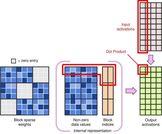](https://mlsysbook.ai/contents/core/optimizations/8ac206f360f289b450ef2f7d051d197eedcfc31b.svg "Figure 28: Block Sparse Representation: NVIDIA’s cusparse library efficiently stores block sparse matrices by exploiting dense submatrix structures, enabling accelerated matrix operations while maintaining compatibility with dense matrix computations through block indexing. this approach reduces memory footprint and arithmetic complexity for sparse linear algebra, important for scaling machine learning models. source: NVIDIA..")
Figure 28: **Block Sparse Representation**: NVIDIA’s cusparse library efficiently stores block sparse matrices by exploiting dense submatrix structures, enabling accelerated matrix operations while maintaining compatibility with dense matrix computations through block indexing. this approach reduces memory footprint and arithmetic complexity for sparse linear algebra, important for scaling machine learning models. _source: NVIDIA._.
Similarly, the \\(N\\):\\(M\\) sparsity pattern is a structured sparsity format where, in every set of \\(M\\) consecutive elements (e.g., weights or activations), exactly \\(N\\) are non-zero, and the other two are zero ([Zhou et al. 2021](https://mlsysbook.ai/contents/core/optimizations/optimizations.html#ref-zhou2021learningnmfinegrainedstructured)
). This deterministic pattern facilitates efficient hardware acceleration, as it allows for predictable memory access patterns and optimized computations. By enforcing this structure, models can achieve a balance between sparsity-induced efficiency gains and maintaining sufficient capacity for learning complex representations. [Figure 29](https://mlsysbook.ai/contents/core/optimizations/optimizations.html#fig-2-4-gemm)
below shows a comparison between accelerating dense versus 2:4 sparsity matrix multiplication, a common sparsity pattern used in model training. Later works like STEP ([Lu et al. 2023](https://mlsysbook.ai/contents/core/optimizations/optimizations.html#ref-lu2023steplearningnmstructured)
) have examined learning more general \\(N\\):\\(M\\) sparsity masks for accelerating deep learning inference under the same principles.
Zhou, Aojun, Yukun Ma, Junnan Zhu, Jianbo Liu, Zhijie Zhang, Kun Yuan, Wenxiu Sun, and Hongsheng Li. 2021. “Learning n:m Fine-Grained Structured Sparse Neural Networks from Scratch,” February. [http://arxiv.org/abs/2102.04010v2](http://arxiv.org/abs/2102.04010v2)
.
Lu, Yucheng, Shivani Agrawal, Suvinay Subramanian, Oleg Rybakov, Christopher De Sa, and Amir Yazdanbakhsh. 2023. “STEP: Learning n:m Structured Sparsity Masks from Scratch with Precondition,” February. [http://arxiv.org/abs/2302.01172v1](http://arxiv.org/abs/2302.01172v1)
.
[](https://mlsysbook.ai/contents/core/optimizations/d34ae57d8b9cb0954a8645a52a87c4036b1ab621.svg "Figure 29: Sparse Matrix Multiplication: Block sparsity optimizes matrix operations by storing only non-zero elements and using structured indexing, enabling efficient GPU acceleration for neural network computations. this technique maintains compatibility with dense matrix operations while reducing memory access and computational cost, particularly beneficial for large-scale models. source: PyTorch blog.")
Figure 29: **Sparse Matrix Multiplication**: Block sparsity optimizes matrix operations by storing only non-zero elements and using structured indexing, enabling efficient GPU acceleration for neural network computations. this technique maintains compatibility with dense matrix operations while reducing memory access and computational cost, particularly beneficial for large-scale models. source: [PyTorch blog](https://pytorch.org/blog/accelerating-neural-network-training/)
.
##### GPUs and Sparse Operations
Graphics Processing Units (GPUs) are widely recognized for their ability to perform highly parallel computations, making them ideal for handling the large-scale matrix operations that are common in machine learning. Modern GPUs, such as NVIDIA’s Ampere architecture, include specialized Sparse Tensor Cores that accelerate sparse matrix multiplications. These tensor cores are designed to recognize and skip over zero elements in sparse matrices, thereby reducing the number of operations required ([Abdelkhalik et al. 2022](https://mlsysbook.ai/contents/core/optimizations/optimizations.html#ref-NVIDIA2020)
). This is particularly advantageous for structured pruning techniques, where entire filters, channels, or layers are pruned, resulting in a significant reduction in the amount of computation. By skipping over the zero values, GPUs can speed up matrix multiplications by a factor of two or more, resulting in lower processing times and reduced power consumption for sparse networks.
Abdelkhalik, Hamdy, Yehia Arafa, Nandakishore Santhi, and Abdel-Hameed A. Badawy. 2022. “Demystifying the Nvidia Ampere Architecture Through Microbenchmarking and Instruction-Level Analysis.” In _2022 IEEE High Performance Extreme Computing Conference (HPEC)_. IEEE. [https://doi.org/10.1109/hpec55821.2022.9926299](https://doi.org/10.1109/hpec55821.2022.9926299)
.
Hoefler, Torsten, Dan Alistarh, Tal Ben-Nun, Nikoli Dryden, and Alexandra Peste. 2021. “Sparsity in Deep Learning: Pruning and Growth for Efficient Inference and Training in Neural Networks.” _arXiv Preprint arXiv:2102.00554_ 22 (January): 1–124. [http://arxiv.org/abs/2102.00554v1](http://arxiv.org/abs/2102.00554v1)
.
GPUs leverage their parallel architecture to handle multiple operations simultaneously. This parallelism is especially beneficial for sparse operations, as it allows the hardware to exploit the inherent sparsity in the data more efficiently. However, the full benefit of sparse operations on GPUs requires that the sparsity is structured in a way that aligns with the underlying hardware architecture, making structured pruning more advantageous for optimization ([Hoefler, Alistarh, Ben-Nun, Dryden, and Peste 2021](https://mlsysbook.ai/contents/core/optimizations/optimizations.html#ref-Hoefler2021)
).
##### TPUs and Sparse Optimization
TPUs, developed by Google, are custom-built hardware accelerators specifically designed to handle tensor computations at a much higher efficiency than traditional processors. TPUs, such as TPU v4, have built-in support for sparse weight matrices, which is particularly beneficial for models like transformers, including BERT and GPT, that rely on large-scale matrix multiplications ([Jouppi et al. 2021](https://mlsysbook.ai/contents/core/optimizations/optimizations.html#ref-Jouppi2021)
). TPUs optimize sparse weight matrices by reducing the computational load associated with zero elements, enabling faster processing and improved energy efficiency.
Jouppi, Norman P., Doe Hyun Yoon, Matthew Ashcraft, Mark Gottscho, Thomas B. Jablin, George Kurian, James Laudon, et al. 2021. “Ten Lessons from Three Generations Shaped Google’s TPUv4i : Industrial Product.” In _2021 ACM/IEEE 48th Annual International Symposium on Computer Architecture (ISCA)_, 1–14. IEEE. [https://doi.org/10.1109/isca52012.2021.00010](https://doi.org/10.1109/isca52012.2021.00010)
.
The efficiency of TPUs comes from their ability to perform operations at high throughput and low latency, thanks to their custom-designed matrix multiply units. These units are able to accelerate sparse matrix operations by directly processing the non-zero elements, making them well-suited for models that incorporate significant sparsity, whether through pruning or low-rank approximations. As the demand for larger models increases, TPUs continue to play a important role in maintaining performance while minimizing the energy and computational cost associated with dense computations.
##### FPGAs and Sparse Computations
Field-Programmable Gate Arrays (FPGAs) are another important class of hardware accelerators for sparse networks. Unlike GPUs and TPUs, FPGAs are highly customizable, offering flexibility in their design to optimize specific computational tasks. This makes them particularly suitable for sparse operations that require fine-grained control over hardware execution. FPGAs can be programmed to perform sparse matrix-vector multiplications and other sparse matrix operations with minimal overhead, delivering high performance for models that use unstructured pruning or require custom sparse patterns.
One of the main advantages of FPGAs in sparse networks is their ability to be tailored for specific applications, which allows for optimizations that general-purpose hardware cannot achieve. For instance, an FPGA can be designed to skip over zero elements in a matrix by customizing the data path and memory management, providing significant savings in both computation and memory usage. FPGAs also allow for low-latency execution, making them well-suited for real-time applications that require efficient processing of sparse data streams.
##### Memory and Energy Optimization
One of the key challenges in sparse networks is managing memory bandwidth, as matrix operations often require significant memory access. Sparse networks offer a solution by reducing the number of elements that need to be accessed, thus minimizing memory traffic. Hardware accelerators detailed in **[Chapter 11: AI Acceleration](https://mlsysbook.ai/contents/core/hw_acceleration/hw_acceleration.html#sec-ai-acceleration)
** are optimized for these sparse matrices, utilizing specialized memory access patterns that skip zero values, reducing the total amount of memory bandwidth used ([Baraglia and Konno 2019](https://mlsysbook.ai/contents/core/optimizations/optimizations.html#ref-Gale2020)
).
Baraglia, David, and Hokuto Konno. 2019. “On the Bauer-Furuta and Seiberg-Witten Invariants of Families of \\(4\\)\-Manifolds.” _arXiv Preprint arXiv:1903.01649_, March, 8955–67. [http://arxiv.org/abs/1903.01649v3](http://arxiv.org/abs/1903.01649v3)
.
For example, GPUs and TPUs are designed to minimize memory access latency by taking advantage of their high memory bandwidth. By accessing only non-zero elements, these accelerators ensure that memory is used more efficiently. The memory hierarchies in these devices are also optimized for sparse computations, allowing for faster data retrieval and reduced power consumption.
The reduction in the number of computations and memory accesses directly translates into energy savings[39](https://mlsysbook.ai/contents/core/optimizations/optimizations.html#fn39)
. Sparse operations require fewer arithmetic operations and fewer memory fetches, leading to a decrease in the energy consumption required for both training and inference. This energy efficiency is particularly important for applications that run on edge devices, where power constraints are important, as explored in **[Chapter 14: On-Device Learning](https://mlsysbook.ai/contents/core/ondevice_learning/ondevice_learning.html#sec-ondevice-learning)
**.
39 **Sparse Energy Savings**: 90% sparsity in BERT reduces training energy by 2.3x and inference energy by 4.1x on V100. Structured 2:4 sparsity patterns deliver 1.6x energy savings on A100 GPUs while maintaining 99% of dense model accuracy. Hardware accelerators like TPUs and GPUs are optimized to handle these operations efficiently, making sparse networks not only faster but also more energy-efficient ([Cheng et al. 2022](https://mlsysbook.ai/contents/core/optimizations/optimizations.html#ref-Cheng2022)
).
Cheng, Yu et al. 2022. “Memory-Efficient Deep Learning: Advances in Model Compression and Sparsification.” _ACM Computing Surveys_.
##### Future: Hardware and Sparse Networks
As hardware continues to evolve, we can expect more innovations tailored specifically for sparse networks. Future hardware accelerators may offer deeper integration with sparsity-aware training and optimization algorithms, allowing even greater reductions in computational and memory costs. Emerging fields like neuromorphic computing, inspired by the brain’s structure, may provide new avenues for processing sparse networks in energy-efficient ways ([Davies et al. 2021](https://mlsysbook.ai/contents/core/optimizations/optimizations.html#ref-Davies2021)
). These advancements promise to further enhance the efficiency and scalability of machine learning models, particularly in applications that require real-time processing and run on power-constrained devices, connecting to the sustainable AI principles in **[Chapter 18: Sustainable AI](https://mlsysbook.ai/contents/core/sustainable_ai/sustainable_ai.html#sec-sustainable-ai)
**.
Davies, Mike et al. 2021. “Advancing Neuromorphic Computing with Sparse Networks.” _Nature Electronics_.
#### Challenges and Limitations
While exploiting sparsity offers significant advantages in reducing computational cost and memory usage, several challenges and limitations must be considered for the effective implementation of sparse networks. [Table 11](https://mlsysbook.ai/contents/core/optimizations/optimizations.html#tbl-sparsity-optimization)
summarizes some of the challenges and limitations associated with sparsity optimizations.
Table 11: **Sparsity Optimization Challenges**: Unstructured sparsity, while reducing model size, hinders hardware acceleration due to irregular memory access patterns, limiting potential computational savings and requiring specialized hardware or software to realize efficiency gains. This table summarizes key challenges in effectively deploying sparse neural networks.
| | | |
| --- | --- | --- |
| **Unstructured Sparsity Optimization** | Irregular sparse patterns make it difficult to exploit sparsity on hardware. | Limited hardware acceleration and reduced computational savings. |
| **Algorithmic Complexity** | Sophisticated pruning and sparse matrix operations require complex algorithms. | High computational overhead and algorithmic complexity for large models. |
| **Hardware Support** | Hardware accelerators are optimized for structured sparsity, making unstructured sparsity harder to optimize. | Suboptimal hardware utilization and lower performance for unstructured sparsity. |
| **Accuracy Trade-off** | Aggressive sparsity may degrade model accuracy if not carefully balanced. | Potential loss in performance, requiring careful tuning and validation. |
| **Energy Efficiency** | Overhead from sparse matrix storage and management can offset the energy savings from reduced computation. | Power consumption may not improve if the overhead surpasses savings from sparse computations. |
| **Limited Applicability** | Sparsity may not benefit all models or tasks, especially in domains requiring dense representations. | Not all models or hardware benefit equally from sparsity. |
One of the main challenges of sparsity is the optimization of unstructured sparsity. In unstructured pruning, individual weights are removed based on their importance, leading to an irregular sparse pattern. This irregularity makes it difficult to fully exploit the sparsity on hardware, as most hardware accelerators (like GPUs and TPUs) are designed to work more efficiently with structured data. Without a regular structure, these accelerators may not be able to skip zero elements as effectively, which can limit the computational savings.
Another challenge is the algorithmic complexity involved in pruning and sparse matrix operations. The process of deciding which weights to prune, particularly in an unstructured manner, requires sophisticated algorithms that must balance model accuracy with computational efficiency. These pruning algorithms can be computationally expensive themselves, and applying them across large models can result in significant overhead. The optimization of sparse matrices also requires specialized techniques that may not always be easy to implement or generalize across different architectures.
Hardware support is another important limitation. Although modern GPUs, TPUs, and FPGAs have specialized features designed to accelerate sparse operations, fully optimizing sparse networks on hardware requires careful alignment between the hardware architecture and the sparsity format. While structured sparsity is easier to leverage on these accelerators, unstructured sparsity remains a challenge, as hardware accelerators may struggle to efficiently handle irregular sparse patterns. Even when hardware is optimized for sparse operations, the overhead associated with sparse matrix storage formats and the need for specialized memory management can still result in suboptimal performance.
There is always a trade-off between sparsity and accuracy. Aggressive pruning or low-rank approximation techniques that aggressively reduce the number of parameters can lead to accuracy degradation. Finding the right balance between reducing parameters and maintaining high model performance is a delicate process that requires extensive experimentation. In some cases, introducing too much sparsity can result in a model that is too small or too underfit to achieve high performance.
While sparsity can lead to energy savings, energy efficiency is not always guaranteed. Although sparse operations require fewer floating-point operations, the overhead of managing sparse data and ensuring that hardware optimally skips over zero values can introduce additional power consumption. In edge devices or mobile environments with tight power budgets, the benefits of sparsity may be less clear if the overhead associated with sparse data structures and hardware utilization outweighs the energy savings.
There is a limited applicability of sparsity to certain types of models or tasks. Not all models benefit equally from sparsity, especially those where dense representations are important for performance. For example, models in domains such as image segmentation or some types of reinforcement learning may not show significant gains when sparsity is introduced. Sparsity may not be effective for all hardware platforms, particularly for older or lower-end devices that lack the computational power or specialized features required to take advantage of sparse matrix operations.
#### Combined Optimizations
While sparsity in neural networks is a powerful technique for improving computational efficiency and reducing memory usage, its full potential is often realized when it is used alongside other optimization strategies. These optimizations include techniques like pruning, quantization, and efficient model design. Understanding how sparsity interacts with these methods is important for effectively combining them to achieve optimal performance ([Hoefler, Alistarh, Ben-Nun, Dryden, and Ziogas 2021](https://mlsysbook.ai/contents/core/optimizations/optimizations.html#ref-hoefler2021sparsity)
).
Hoefler, Torsten, Dan Alistarh, Tal Ben-Nun, Nikoli Dryden, and Alexandros Nikolaos Ziogas. 2021. “Sparsity in Deep Learning: Pruning and Growth for Efficient Inference and Training in Neural Networks.” _Journal of Machine Learning Research_ 22 (241): 1–124.
##### Sparsity and Pruning
Pruning and sparsity are closely related techniques. When pruning is applied, the resulting model may become sparse, but the sparsity pattern, such as whether it is structured or unstructured, affects how effectively the model can be optimized for hardware. For example, structured pruning (e.g., pruning entire filters or layers) typically results in more efficient sparsity, as hardware accelerators like GPUs and TPUs are better equipped to handle regular patterns in sparse matrices ([Elsen et al. 2020](https://mlsysbook.ai/contents/core/optimizations/optimizations.html#ref-elsen2020fast)
). Unstructured pruning, on the other hand, can introduce irregular sparsity patterns, which may not be as efficiently processed by hardware, especially when combined with other techniques like quantization.
Pruning-generated sparse patterns must align with underlying hardware architecture to achieve computational savings ([Gale, Elsen, and Hooker 2019b](https://mlsysbook.ai/contents/core/optimizations/optimizations.html#ref-gale2019state)
). Structured pruning proves particularly effective for hardware optimization.
##### Sparsity and Quantization
Combining sparsity and quantization yields significant reductions in memory usage and computation, but presents unique challenges ([Nagel et al. 2021a](https://mlsysbook.ai/contents/core/optimizations/optimizations.html#ref-nagel2021white)
). Unstructured sparsity exacerbates low-precision weight processing challenges, particularly on hardware lacking efficient support for irregular sparse matrices. GPUs and TPUs amplify sparse matrix acceleration when combined with low-precision arithmetic, while CPUs struggle with combined overhead ([Zhang et al. 2021](https://mlsysbook.ai/contents/core/optimizations/optimizations.html#ref-zhang2021learning)
).
Nagel, Markus, Marios Fournarakis, Rana Ali Amjad, Yelysei Bondarenko, Mart van Baalen, and Tijmen Blankevoort. 2021a. “A White Paper on Neural Network Quantization.” _arXiv Preprint arXiv:2106.08295_, June. [http://arxiv.org/abs/2106.08295v1](http://arxiv.org/abs/2106.08295v1)
.
Zhang, Yi, Jianlei Yang, Linghao Song, Yiyu Shi, Yu Wang, and Yuan Xie. 2021. “Learning-Based Efficient Sparsity and Quantization for Neural Network Compression.” _IEEE Transactions on Neural Networks and Learning Systems_ 32 (9): 3980–94.
##### Sparsity and Model Design
Efficient model design creates inherently efficient architectures through techniques like depthwise separable convolutions, low-rank approximation, and dynamic computation. Sparsity amplifies these benefits by further reducing memory and computation requirements ([Dettmers and Zettlemoyer 2019](https://mlsysbook.ai/contents/core/optimizations/optimizations.html#ref-dettmers2019sparse)
). However, efficient sparse models require hardware support for sparse operations to avoid suboptimal performance. Hardware alignment ensures both computational cost and memory usage minimization ([Elsen et al. 2020](https://mlsysbook.ai/contents/core/optimizations/optimizations.html#ref-elsen2020fast)
).
Dettmers, Tim, and Luke Zettlemoyer. 2019. “Sparse Networks from Scratch: Faster Training Without Losing Performance.” _arXiv Preprint arXiv:1907.04840_, July. [http://arxiv.org/abs/1907.04840v2](http://arxiv.org/abs/1907.04840v2)
.
Elsen, Erich, Marat Dukhan, Trevor Gale, and Karen Simonyan. 2020. “Fast Sparse ConvNets.” In _2020 IEEE/CVF Conference on Computer Vision and Pattern Recognition (CVPR)_, 14617–26. IEEE. [https://doi.org/10.1109/cvpr42600.2020.01464](https://doi.org/10.1109/cvpr42600.2020.01464)
.
##### Sparsity and Optimization Challenges
Coordinating sparsity with pruning, quantization, and efficient design involves managing accuracy trade-offs ([Labarge, n.d.](https://mlsysbook.ai/contents/core/optimizations/optimizations.html#ref-blalock2020state)
). Hardware accelerators like GPUs and TPUs optimize for structured sparsity but struggle with unstructured patterns or sparsity-quantization combinations. Optimal performance requires selecting appropriate technique combinations aligned with hardware capabilities ([Gale, Elsen, and Hooker 2019b](https://mlsysbook.ai/contents/core/optimizations/optimizations.html#ref-gale2019state)
), carefully balancing model accuracy, computational cost, memory usage, and hardware efficiency.
Labarge, Isaac E. n.d. “Neural Network Pruning for ECG Arrhythmia Classification.” _Proceedings of Machine Learning and Systems (MLSys)_. PhD thesis, California Polytechnic State University. [https://doi.org/10.15368/theses.2020.76](https://doi.org/10.15368/theses.2020.76)
.
Gale, Trevor, Erich Elsen, and Sara Hooker. 2019b. “The State of Sparsity in Deep Neural Networks.” _arXiv Preprint arXiv:1902.09574_, February. [http://arxiv.org/abs/1902.09574v1](http://arxiv.org/abs/1902.09574v1)
.
**Self-Check: Question 1.8**
1. Which of the following best describes the goal of architectural efficiency optimization in machine learning systems?
1. Aligning model operations with hardware capabilities
2. Improving numerical precision of computations
3. Increasing the number of model parameters
4. Enhancing the theoretical accuracy of models
2. Explain how hardware-aware design principles can improve the deployment efficiency of machine learning models.
3. Which architectural efficiency technique involves reducing memory traffic by combining operations?
1. Dynamic computation strategies
2. Sparsity exploitation techniques
3. Operator fusion methods
4. Hardware-aware design
4. In a production system, what trade-offs would you consider when implementing dynamic computation strategies?
[See Answers →](https://mlsysbook.ai/contents/core/optimizations/optimizations.html#quiz-answer-sec-model-optimizations-architectural-efficiency-techniques-ba84)
Implementation Strategy and Evaluation
--------------------------------------
We now examine systematic application strategies. The individual techniques we have studied rarely succeed in isolation; production systems typically employ coordinated optimization strategies that balance multiple constraints simultaneously. Effective deployment requires structured approaches for profiling systems, measuring optimization impact, and combining techniques to achieve deployment goals.
This section provides methodological guidance for moving from theoretical understanding to practical implementation, addressing three critical questions: Where should optimization efforts focus? How do we measure whether optimizations achieve their intended goals? How do we combine multiple techniques without introducing conflicts or diminishing returns?
### Profiling and Opportunity Analysis
The foundation of optimization lies in thorough profiling to identify where computational resources are being consumed and which components offer the greatest optimization potential. However, a critical first step is determining whether model optimization will actually improve system performance, as model computation often represents only a fraction of total system overhead in production environments.
Modern machine learning models exhibit heterogeneous resource consumption patterns, where specific layers, operations, or data paths contribute disproportionately to memory usage, computational cost, or latency. Understanding these patterns is important for prioritizing optimization efforts and achieving maximum impact with minimal accuracy degradation.
Effective profiling begins with establishing baseline measurements across all relevant performance dimensions. Memory profiling reveals both static memory consumption (model parameters and buffers) and dynamic memory allocation patterns during training and inference. Computational profiling identifies bottleneck operations, typically measured in FLOPS and actual wall-clock execution time. Energy profiling becomes important for battery-powered and edge deployment scenarios, where power consumption directly impacts operational feasibility. Latency profiling measures end-to-end response times and identifies which operations contribute most to inference delay.
Consider profiling a Vision Transformer (ViT) for edge deployment. Using PyTorch Profiler reveals attention layers consuming 65% of total FLOPs (highly amenable to structured pruning), layer normalization consuming 8% of latency despite only 2% of FLOPs (memory-bound operation), and the final classification head consuming 1% of computation but 15% of parameter memory. This profile suggests applying magnitude-based pruning to attention layers as priority one (high FLOP reduction potential), quantizing the classification head to INT8 as priority two (large memory savings, minimal accuracy impact), and fusing layer normalization operations as priority three (reduces memory bandwidth bottleneck).
Extending beyond these baseline measurements, modern optimization requires understanding model sensitivity to different types of modifications. Not all parameters contribute equally to model accuracy, and structured sensitivity analysis helps identify which components can be optimized aggressively versus those that require careful preservation. Layer-wise sensitivity analysis reveals which network components are most important for maintaining accuracy, guiding decisions about where to apply aggressive pruning or quantization versus where to use conservative approaches.
### Measuring Optimization Effectiveness
Optimization requires rigorous measurement frameworks that go beyond simple accuracy metrics to capture the full impact of optimization decisions. Effective measurement considers multiple objectives simultaneously, including accuracy preservation, computational efficiency gains, memory reduction, latency improvement, and energy savings. The challenge lies in balancing these often-competing objectives while maintaining structured decision-making processes.
The measurement framework should establish clear baselines before applying any optimizations, capturing thorough performance profiles across all relevant metrics. Accuracy baselines include not only top-line metrics like classification accuracy but also more nuanced measures such as calibration, fairness across demographic groups, and robustness to input variations. Efficiency baselines capture computational cost (FLOPS, memory bandwidth), actual execution time across different hardware platforms, peak memory consumption during training and inference, and energy consumption profiles.
When quantizing ResNet-50 from FP32 to INT8, baseline metrics show Top-1 accuracy of 76.1%, inference latency on V100 of 4.2ms, model size of 98MB, and energy per inference of 0.31J. Post-quantization metrics reveal Top-1 accuracy of 75.8% (0.3% degradation), inference latency of 1.3ms (3.2x speedup), model size of 25MB (3.9x reduction), and energy per inference of 0.08J (3.9x improvement). Additional analysis shows per-class accuracy degradation ranging from 0.1% to 1.2% with highest impact on fine-grained categories, calibration error increasing from 2.1% to 3.4%, and INT8 quantization providing 3.2x speedup on GPU but only 1.8x on CPU, demonstrating hardware-dependent gains.
With these comprehensive baselines in place, the measurement framework must track optimization impact systematically. Rather than evaluating techniques in isolation, applying our three-dimensional framework requires understanding how different approaches interact when combined. Sequential application can lead to compounding benefits or unexpected interactions that diminish overall effectiveness.
### Multi-Technique Integration Strategies
The most significant optimization gains emerge from combining multiple techniques across our three-dimensional framework. Model representation techniques (pruning) reduce parameter count, numerical precision techniques (quantization) reduce computational cost per operation, and architectural efficiency techniques (operator fusion, dynamic computation) reduce execution overhead. These techniques operate at different optimization dimensions, providing multiplicative benefits when sequenced appropriately.
Sequencing critically impacts results. Consider deploying BERT-Base on mobile devices through three stages. Stage one applies structured pruning, removing 30% of attention heads and 40% of intermediate FFN dimensions, resulting in 75% parameter reduction with accuracy dropping from 76.2% to 75.1%. Stage two uses knowledge distillation to recover accuracy to 75.9%. Stage three applies quantization-aware training with INT8 quantization, achieving 4x additional memory reduction with final accuracy of 75.6%. The combined impact shows 16x memory reduction (440MB to 28MB), 12x inference speedup on mobile CPU, and 0.6% final accuracy loss versus 2.1% if quantization had been applied before pruning.
This example illustrates why sequencing matters: pruning first concentrates important weights into smaller ranges, making subsequent quantization more effective. Applying quantization before pruning reduces numerical precision available for importance-based pruning decisions, degrading final accuracy. Effective combination requires understanding these dependencies and developing application sequences that maximize cumulative benefits. Modern automated approaches, explored in the following AutoML section, leverage our dimensional framework to discover effective technique combinations systematically.
**Self-Check: Question 1.9**
1. Which of the following is a critical first step in the optimization process for machine learning systems?
1. Applying quantization to reduce model size
2. Conducting sensitivity analysis on model parameters
3. Implementing structured pruning techniques
4. Establishing baseline measurements through profiling
2. True or False: In a production environment, model computation often represents the majority of system overhead.
3. Explain how a systematic measurement framework can help balance competing optimization objectives in ML systems.
4. Order the following stages of deploying BERT-Base on mobile devices: (1) Quantization-aware training, (2) Structured pruning, (3) Knowledge distillation.
5. In a production system, what trade-offs would you consider when integrating multiple optimization techniques?
[See Answers →](https://mlsysbook.ai/contents/core/optimizations/optimizations.html#quiz-answer-sec-model-optimizations-implementation-strategy-evaluation-a052)
AutoML and Automated Optimization Strategies
--------------------------------------------
As machine learning models grow in complexity, optimizing them for real-world deployment requires balancing multiple factors, including accuracy, efficiency, and hardware constraints. We have explored various optimization techniques, including pruning, quantization, and neural architecture search, each of which targets specific aspects of model efficiency. However, applying these optimizations effectively often requires extensive manual effort, domain expertise, and iterative experimentation.
Automated Machine Learning (AutoML) aims to streamline this process by automating the search for optimal model configurations, building on the training methodologies from **[Chapter 8: AI Training](https://mlsysbook.ai/contents/core/training/training.html#sec-ai-training)
**. AutoML frameworks leverage machine learning algorithms to optimize architectures, hyperparameters, model compression techniques, and other important parameters, reducing the need for human intervention ([Hutter, Kotthoff, and Vanschoren 2019](https://mlsysbook.ai/contents/core/optimizations/optimizations.html#ref-Hutter2019)
). By systematically exploring the vast design space of possible models, AutoML can improve efficiency while maintaining competitive accuracy, often discovering novel solutions that may be overlooked through manual tuning ([Zoph and Le 2017b](https://mlsysbook.ai/contents/core/optimizations/optimizations.html#ref-Zoph2017)
).
Hutter, Frank, Lars Kotthoff, and Joaquin Vanschoren. 2019. _Automated Machine Learning: Methods, Systems, Challenges_. Springer International Publishing. [https://doi.org/10.1007/978-3-030-05318-5](https://doi.org/10.1007/978-3-030-05318-5)
.
AutoML does not replace the need for human expertise but rather enhances it by providing a structured and scalable approach to model optimization. As illustrated in [Figure 30](https://mlsysbook.ai/contents/core/optimizations/optimizations.html#fig-automl-comparison)
, the key difference between traditional workflows and AutoML is that preprocessing, training and evaluation are automated in the latter. Instead of manually adjusting pruning thresholds, quantization strategies, or architecture designs, practitioners can define high-level objectives, including latency constraints, memory limits, and accuracy targets, and allow AutoML systems to explore configurations that best satisfy these constraints ([Feurer et al. 2019](https://mlsysbook.ai/contents/core/optimizations/optimizations.html#ref-Feurer2015)
), enabling the robust deployment strategies detailed in **[Chapter 16: Robust AI](https://mlsysbook.ai/contents/core/robust_ai/robust_ai.html#sec-robust-ai)
**.
[](https://mlsysbook.ai/contents/core/optimizations/f028f47c9cc1c052d91008292eb3505f15e4ad88.svg "Figure 30: AutoML Workflow: Automated machine learning (automl) streamlines model development by structurally automating data preprocessing, model selection, and hyperparameter tuning, contrasting with traditional workflows requiring extensive manual effort for each stage. This automation enables practitioners to define high-level objectives and constraints, allowing automl systems to efficiently explore a vast design space and identify optimal model configurations.")
Figure 30: **AutoML Workflow**: Automated machine learning (automl) streamlines model development by structurally automating data preprocessing, model selection, and hyperparameter tuning, contrasting with traditional workflows requiring extensive manual effort for each stage. This automation enables practitioners to define high-level objectives and constraints, allowing automl systems to efficiently explore a vast design space and identify optimal model configurations.
This section explores the core aspects of AutoML, starting with the key dimensions of optimization, followed by the methodologies used in AutoML systems, and concluding with challenges and limitations. This examination reveals how AutoML serves as an integrative framework that unifies many of the optimization strategies discussed earlier.
### AutoML Optimizations
AutoML is designed to optimize multiple aspects of a machine learning model, ensuring efficiency, accuracy, and deployability. Unlike traditional approaches that focus on individual techniques, such as quantization for reducing numerical precision or pruning for compressing models, AutoML takes a holistic approach by jointly considering these factors. This enables a more thorough search for optimal model configurations, balancing performance with real-world constraints ([Y. He et al. 2018](https://mlsysbook.ai/contents/core/optimizations/optimizations.html#ref-He2018)
).
He, Yihui, Ji Lin, Zhijian Liu, Hanrui Wang, Li-Jia Li, and Song Han. 2018. “AMC: AutoML for Model Compression and Acceleration on Mobile Devices.” In _Computer Vision – ECCV 2018_, 815–32. Springer International Publishing. [https://doi.org/10.1007/978-3-030-01234-2\\\_48](https://doi.org/10.1007/978-3-030-01234-2/_48)
.
Elsken, Thomas, Jan Hendrik Metzen, and Frank Hutter. 2019b. “Neural Architecture Search.” In _Automated Machine Learning_, 63–77. Springer International Publishing. [https://doi.org/10.1007/978-3-030-05318-5\\\_3](https://doi.org/10.1007/978-3-030-05318-5/_3)
.
Tan, Mingxing, and Quoc V. Le. 2019b. “EfficientNet: Rethinking Model Scaling for Convolutional Neural Networks.” In _International Conference on Machine Learning_.
One of the primary optimization targets of AutoML is neural network architecture search. Designing an efficient model architecture is a complex process that requires balancing layer configurations, connectivity patterns, and computational costs. NAS automates this by structuredally exploring different network structures, evaluating their efficiency, and selecting the most optimal design ([Elsken, Metzen, and Hutter 2019b](https://mlsysbook.ai/contents/core/optimizations/optimizations.html#ref-Elsken2019)
). This process has led to the discovery of architectures such as MobileNetV3 and EfficientNet, which outperform manually designed models on key efficiency metrics ([Tan and Le 2019b](https://mlsysbook.ai/contents/core/optimizations/optimizations.html#ref-Tan2019)
).
Beyond architecture design, AutoML also focuses on hyperparameter optimization[40](https://mlsysbook.ai/contents/core/optimizations/optimizations.html#fn40)
, which plays a important role in determining a model’s performance. Parameters such as learning rate, batch size[41](https://mlsysbook.ai/contents/core/optimizations/optimizations.html#fn41)
, weight decay, and activation functions must be carefully tuned for stability and efficiency.
40 **Hyperparameter Optimization**: Learning rate search alone can improve model accuracy by 5-15%. Grid search over 4 hyperparameters with 10 values each requires 10,000 training runs. Bayesian optimization reduces this to 100-200 runs while achieving comparable results, saving weeks of computation.
41 **Batch Size Effects**: Large batches (512-2048) improve throughput by 2-4x but require gradient accumulation for memory constraints. Linear scaling rule maintains convergence: learning rate scales linearly with batch size, enabling ImageNet training in 1 hour with batch size 8192.
42 **Bayesian Optimization**: Uses probabilistic models to guide hyperparameter search, modeling objective function uncertainty. Requires 10-50x fewer evaluations than random search. GPyOpt and Optuna frameworks enable practical Bayesian optimization for neural networks with multi-objective constraints.
Bardenet, Rémi, Olivier Cappé, Gersende Fort, and Balázs Kégl. 2015. “Adaptive MCMC with Online Relabeling.” _Bernoulli_ 21 (3). [https://doi.org/10.3150/13-bej578](https://doi.org/10.3150/13-bej578)
.
Instead of relying on trial and error, AutoML frameworks employ structured search strategies, including Bayesian optimization[42](https://mlsysbook.ai/contents/core/optimizations/optimizations.html#fn42)
, evolutionary algorithms, and adaptive heuristics, to efficiently identify the best hyperparameter settings for a given model and dataset ([Bardenet et al. 2015](https://mlsysbook.ai/contents/core/optimizations/optimizations.html#ref-Bergstra2011)
).
Another important aspect of AutoML is model compression. Techniques such as pruning and quantization help reduce the memory footprint and computational requirements of a model, making it more suitable for deployment on resource-constrained hardware. AutoML frameworks automate the selection of pruning thresholds, sparsity patterns, and quantization levels, optimizing models for both speed and energy efficiency ([Jiaxiang Wu et al. 2016](https://mlsysbook.ai/contents/core/optimizations/optimizations.html#ref-Wu2016)
). This is particularly important for edge AI applications, where models need to operate with minimal latency and power consumption ([Chowdhery et al. 2021](https://mlsysbook.ai/contents/core/optimizations/optimizations.html#ref-Chowdhery2021)
).
Wu, Jiaxiang, Cong Leng, Yuhang Wang, Qinghao Hu, and Jian Cheng. 2016. “Quantized Convolutional Neural Networks for Mobile Devices.” In _2016 IEEE Conference on Computer Vision and Pattern Recognition (CVPR)_, 4820–28. IEEE. [https://doi.org/10.1109/cvpr.2016.521](https://doi.org/10.1109/cvpr.2016.521)
.
Chowdhery, Aakanksha, Anatoli Noy, Gaurav Misra, Zhuyun Dai, Quoc V. Le, and Jeff Dean. 2021. “Edge TPU: An Edge-Optimized Inference Accelerator for Deep Learning.” In _International Symposium on Computer Architecture_.
Cai, Han, Chuang Gan, and Song Han. 2020. “Once-for-All: Train One Network and Specialize It for Efficient Deployment.” In _International Conference on Learning Representations_.
Finally, AutoML considers deployment-aware optimization, ensuring that the final model is suited for real-world execution. Different hardware platforms impose varying constraints on model execution, such as memory bandwidth limitations, computational throughput, and energy efficiency requirements. AutoML frameworks incorporate hardware-aware optimization techniques, tailoring models to specific devices by adjusting computational workloads, memory access patterns, and execution strategies ([Cai, Gan, and Han 2020](https://mlsysbook.ai/contents/core/optimizations/optimizations.html#ref-Cai2020)
).
Optimization across these dimensions enables AutoML to provide a unified framework for enhancing machine learning models, streamlining the process to achieve efficiency without sacrificing accuracy. This holistic approach ensures that models are not only theoretically optimal but also practical for real-world deployment across diverse applications and hardware platforms.
### Optimization Strategies
AutoML systems systematically explore different configurations to identify optimal combinations of architectures, hyperparameters, and compression strategies. Unlike manual tuning requiring extensive domain expertise, AutoML leverages algorithmic search methods to navigate the vast design space while balancing accuracy, efficiency, and deployment constraints.
NAS forms the foundation of AutoML by automating architecture design through reinforcement learning, evolutionary algorithms, and gradient-based optimization ([Zoph and Le 2017b](https://mlsysbook.ai/contents/core/optimizations/optimizations.html#ref-Zoph2017)
). By systematically evaluating candidate architectures, NAS identifies structures that outperform manually designed models ([Real et al. 2019](https://mlsysbook.ai/contents/core/optimizations/optimizations.html#ref-Real2019)
). Hyperparameter optimization (HPO) complements this by fine-tuning training parameters—learning rate, batch size, weight decay—using Bayesian optimization and adaptive heuristics that converge faster than grid search ([Feurer et al. 2019](https://mlsysbook.ai/contents/core/optimizations/optimizations.html#ref-Feurer2015)
).
Zoph, Barret, and Quoc V. Le. 2017b. “Neural Architecture Search with Reinforcement Learning.” In _International Conference on Learning Representations_.
Real, Esteban, Alok Aggarwal, Yanping Huang, and Quoc V. Le. 2019. “Regularized Evolution for Image Classifier Architecture Search.” _Proceedings of the AAAI Conference on Artificial Intelligence_ 33 (01): 4780–89. [https://doi.org/10.1609/aaai.v33i01.33014780](https://doi.org/10.1609/aaai.v33i01.33014780)
.
Feurer, Matthias, Aaron Klein, Katharina Eggensperger, Jost Tobias Springenberg, Manuel Blum, and Frank Hutter. 2019. “Auto-Sklearn: Efficient and Robust Automated Machine Learning.” In _Automated Machine Learning_, 113–34. Springer International Publishing. [https://doi.org/10.1007/978-3-030-05318-5\\\_6](https://doi.org/10.1007/978-3-030-05318-5/_6)
.
Model compression optimization automatically selects pruning and quantization strategies based on deployment requirements, evaluating trade-offs between model size, latency, and accuracy. This enables efficient deployment on resource-constrained devices (**[Chapter 14: On-Device Learning](https://mlsysbook.ai/contents/core/ondevice_learning/ondevice_learning.html#sec-ondevice-learning)
**) without manual tuning. Data processing strategies further enhance performance through automated feature selection, adaptive augmentation policies, and dataset balancing that improve robustness (**[Chapter 16: Robust AI](https://mlsysbook.ai/contents/core/robust_ai/robust_ai.html#sec-robust-ai)
**) without computational overhead.
Meta-learning approaches represent recent advances where knowledge from previous optimization tasks accelerates searches for new models ([Vanschoren 2018](https://mlsysbook.ai/contents/core/optimizations/optimizations.html#ref-Vanschoren2019)
). By learning from prior experiments, AutoML systems intelligently explore the optimization space, reducing training and evaluation costs while enabling faster adaptation to new tasks and datasets.
Vanschoren, Joaquin. 2018. “Meta-Learning: A Survey.” _ArXiv Preprint arXiv:1810.03548_, October. [http://arxiv.org/abs/1810.03548v1](http://arxiv.org/abs/1810.03548v1)
.
Li, Lisha, Kevin G. Jamieson, Giulia DeSalvo, Afshin Rostamizadeh, and Ameet Talwalkar. 2017. “Hyperband: A Novel Bandit-Based Approach to Hyperparameter Optimization.” _J. Mach. Learn. Res._ 18: 185:1–52. [https://jmlr.org/papers/v18/16-558.html](https://jmlr.org/papers/v18/16-558.html)
.
Finally, many modern AutoML frameworks offer end-to-end automation, integrating architecture search, hyperparameter tuning, and model compression into a single pipeline. Platforms such as Google AutoML, Amazon SageMaker Autopilot, and Microsoft Azure AutoML provide fully automated workflows that streamline the entire model optimization process ([Li et al. 2017](https://mlsysbook.ai/contents/core/optimizations/optimizations.html#ref-Li2021)
).
The integration of these strategies enables AutoML systems to provide a scalable and efficient approach to model optimization, reducing the reliance on manual experimentation. This automation not only accelerates model development but also enables the discovery of novel architectures and configurations that might otherwise be overlooked, supporting the structured evaluation methods in **[Chapter 12: Benchmarking AI](https://mlsysbook.ai/contents/core/benchmarking/benchmarking.html#sec-benchmarking-ai)
**.
### AutoML Optimization Challenges
While AutoML offers a powerful framework for optimizing machine learning models, it also introduces several challenges and trade-offs that must be carefully considered. Despite its ability to automate model design and hyperparameter tuning, AutoML is not a one-size-fits-all solution. The effectiveness of AutoML depends on computational resources, dataset characteristics, and the specific constraints of a given application.
One of the most significant challenges in AutoML is computational cost. The process of searching for optimal architectures, hyperparameters, and compression strategies requires evaluating numerous candidate models, each of which must be trained and validated. Methods like NAS can be particularly expensive, often requiring thousands of GPU hours to explore a large search space. While techniques such as early stopping, weight sharing, and surrogate models help reduce search costs, the computational overhead remains a major limitation, especially for organizations with limited access to high-performance computing resources.
Another challenge is bias in search strategies, which can influence the final model selection. The optimization process in AutoML is guided by heuristics and predefined objectives, which may lead to biased results depending on how the search space is defined. If the search algorithm prioritizes certain architectures or hyperparameters over others, it may fail to discover alternative configurations that could be more effective for specific tasks. Biases in training data can propagate through the AutoML process, reinforcing unwanted patterns in the final model.
Generalization and transferability present additional concerns. AutoML-generated models are optimized for specific datasets and deployment conditions, but their performance may degrade when applied to new tasks or environments. Unlike manually designed models, where human intuition can guide the selection of architectures that generalize well, AutoML relies on empirical evaluation within a constrained search space. This limitation raises questions about the robustness of AutoML-optimized models when faced with real-world variability.
Interpretability is another key consideration. Many AutoML-generated architectures and configurations are optimized for efficiency but lack transparency in their design choices. Understanding why a particular AutoML-discovered model performs well can be challenging, making it difficult for practitioners to debug issues or adapt models for specific needs. The black-box nature of some AutoML techniques limits human insight into the underlying optimization process.
Beyond technical challenges, there is also a trade-off between automation and control. While AutoML reduces the need for manual intervention, it also abstracts away many decision-making processes that experts might otherwise fine-tune for specific applications. In some cases, domain knowledge is important for guiding model optimization, and fully automated systems may not always account for subtle but important constraints imposed by the problem domain.
Despite these challenges, AutoML continues to evolve, with ongoing research focused on reducing computational costs, improving generalization, and enhancing interpretability. As these improvements emerge, AutoML is expected to play an increasingly prominent role in the development of optimized machine learning models, making AI systems more accessible and efficient for a wide range of applications.
The optimization techniques explored—spanning model representation, numerical precision, architectural efficiency, and automated selection—provide a comprehensive toolkit for efficient machine learning systems. However, practical implementation requires robust software infrastructure bridging the gap between optimization research and deployment through easy-to-use APIs, efficient implementations, and seamless workflow integration.
**Self-Check: Question 1.10**
1. Which of the following best describes the role of AutoML in machine learning model optimization?
1. It completely replaces the need for human expertise in model design.
2. It automates the search for optimal model configurations, reducing manual effort.
3. It focuses solely on improving model accuracy without considering efficiency.
4. It is primarily used for data collection and preprocessing.
2. Explain how AutoML frameworks balance accuracy and efficiency in model optimization.
3. True or False: AutoML can fully eliminate the need for domain expertise in model optimization.
4. The process of automatically selecting pruning thresholds and quantization levels in AutoML is known as \_\_\_\_.
5. In a production system, what trade-offs might you consider when implementing AutoML for model optimization?
[See Answers →](https://mlsysbook.ai/contents/core/optimizations/optimizations.html#quiz-answer-sec-model-optimizations-automl-automated-optimization-strategies-329f)
Implementation Tools and Software Frameworks
--------------------------------------------
The theoretical understanding of model optimization techniques like pruning, quantization, and efficient numerics is important, but their practical implementation relies heavily on robust software support. Without extensive framework development and tooling, these optimization methods would remain largely inaccessible to practitioners. Implementing quantization would require manual modification of model definitions and careful insertion of quantization operations throughout the network. Pruning would involve direct manipulation of weight tensors, tasks that become prohibitively complex as models scale.
Modern machine learning frameworks provide high-level APIs and automated workflows that abstract away implementation complexity, making sophisticated optimization techniques accessible to practitioners. Frameworks address key challenges: providing pre-built modules for common optimization techniques, assisting with hyperparameter tuning (pruning schedules, quantization bit-widths), managing accuracy-compression trade-offs through automated evaluation, and ensuring hardware compatibility through device-specific code generation.
This software infrastructure transforms theoretical optimization techniques into practical tools readily applied in production environments (**[Chapter 13: ML Operations](https://mlsysbook.ai/contents/core/ops/ops.html#sec-ml-operations)
**). Production optimization workflows involve additional considerations including model versioning strategies, monitoring optimization impact on data pipelines, managing optimization artifacts across development and deployment environments, and establishing rollback procedures when optimizations fail. This accessibility bridges the gap between academic research and industrial applications, enabling widespread deployment of efficient machine learning models.
### Model Optimization APIs and Tools
Leading frameworks such as TensorFlow, PyTorch, and MXNet provide comprehensive APIs enabling practitioners to apply optimization techniques without implementing complex algorithms from scratch (**[Chapter 7: AI Frameworks](https://mlsysbook.ai/contents/core/frameworks/frameworks.html#sec-ai-frameworks)
**). These built-in optimizations enhance model efficiency while ensuring adherence to established best practices.
TensorFlow’s Model Optimization Toolkit facilitates quantization, pruning, and clustering. QAT converts floating-point models to lower-precision formats (INT8) while preserving accuracy, systematically managing both weight and activation quantization across diverse architectures. Pruning algorithms introduce sparsity by removing redundant connections at varying granularity levels—individual weights to entire layers—allowing practitioners to tailor strategies to specific requirements. Weight clustering groups similar weights for compression while preserving functionality, providing multiple pathways for improving model efficiency.
Similarly, PyTorch offers thorough optimization support through built-in modules for quantization and pruning. The `torch.quantization` package provides tools for converting models to lower-precision representations, supporting both post-training quantization and quantization-aware training, as shown in [Listing 3](https://mlsysbook.ai/contents/core/optimizations/optimizations.html#lst-qat_example)
.
Listing 3: **Quantization-Aware Training**: Prepares a model to be trained in lower-precision formats, ensuring that quantization errors are accounted for during training.
import torch
from torch.quantization import QuantStub, DeQuantStub,
prepare_qat
# Define a model with quantization support
class QuantizedModel(torch.nn.Module):
def __init__(self):
super().__init__()
self.quant = QuantStub()
self.conv = torch.nn.Conv2d(3, 64, 3)
self.dequant = DeQuantStub()
def forward(self, x):
x = self.quant(x)
x = self.conv(x)
return self.dequant(x)
# Prepare model for quantization-aware training
model = QuantizedModel()
model.qconfig = torch.quantization.get_default_qat_qconfig()
model_prepared = prepare_qat(model)
For pruning, PyTorch provides the `torch.nn.utils.prune` module, which supports both unstructured and structured pruning. An example of both pruning strategies is given in [Listing 4](https://mlsysbook.ai/contents/core/optimizations/optimizations.html#lst-pytorch_pruning)
.
Listing 4: **PyTorch Pruning APIs**: Applies unstructured and structured pruning techniques to reduce model complexity while maintaining performance. _Source: PyTorch Documentation_
import torch.nn.utils.prune as prune
# Apply unstructured pruning
module = torch.nn.Linear(10, 10)
prune.l1_unstructured(module, name="weight", amount=0.3)
# Prune 30% of weights
# Apply structured pruning
prune.ln_structured(module, name="weight", amount=0.5, n=2, dim=0)
These tools integrate seamlessly into PyTorch’s training pipelines, enabling efficient experimentation with different optimization strategies.
Built-in optimization APIs offer significant benefits that make model optimization more accessible and reliable. By providing pre-tested, production-ready tools, these APIs dramatically reduce the implementation complexity that practitioners face when optimizing their models. Rather than having to implement complex optimization algorithms from scratch, developers can leverage standardized interfaces that have been thoroughly vetted.
The consistency provided by these built-in APIs is particularly valuable when working across different model architectures. The standardized interfaces ensure that optimization techniques are applied uniformly, reducing the risk of implementation errors or inconsistencies that could arise from custom solutions. This standardization helps maintain reliable and reproducible results across different projects and teams.
These frameworks also serve as a bridge between cutting-edge research and practical applications. As new optimization techniques emerge from the research community, framework maintainers incorporate these advances into their APIs, making state-of-the-art methods readily available to practitioners. This continuous integration of research advances ensures that developers have access to the latest optimization strategies without needing to implement them independently.
The comprehensive nature of built-in APIs enables rapid experimentation with different optimization approaches. Developers can easily test various strategies, compare their effectiveness, and iterate quickly to find the optimal configuration for their specific use case. This ability to experiment efficiently is important for finding the right balance between model performance and resource constraints.
As model optimization continues to evolve, major frameworks maintain and expand their built-in support, further reducing barriers to efficient model deployment. The standardization of these APIs has played a important role in democratizing access to model efficiency techniques while ensuring high-quality implementations remain consistent and reliable.
### Hardware-Specific Optimization Libraries
Hardware optimization libraries in modern machine learning frameworks covered in **[Chapter 7: AI Frameworks](https://mlsysbook.ai/contents/core/frameworks/frameworks.html#sec-ai-frameworks)
** enable efficient deployment of optimized models across different hardware platforms. These libraries integrate directly with training and deployment pipelines to provide hardware-specific acceleration for various optimization techniques across model representation, numerical precision, and architectural efficiency dimensions.
For model representation optimizations like pruning, libraries such as TensorRT, XLA[43](https://mlsysbook.ai/contents/core/optimizations/optimizations.html#fn43)
, and OpenVINO provide sparsity-aware acceleration through optimized kernels that efficiently handle sparse computations. TensorRT specifically supports structured sparsity patterns, allowing models trained with techniques like two-out-of-four structured pruning to run efficiently on NVIDIA GPUs. Similarly, TPUs leverage XLA’s sparse matrix optimizations, while FPGAs enable custom sparse execution through frameworks like Vitis AI.
43 **XLA (Accelerated Linear Algebra)**: Google’s domain-specific compiler achieves 1.15-1.4x speedup on ResNet-50 inference and 1.2-1.7x on BERT-Large training through operator fusion and memory optimization. XLA reduces HBM traffic by 25-40% through aggressive kernel fusion, delivering 15-30% energy savings on TPUs.
44 **TVM (Tensor Virtual Machine)**: Apache TVM’s auto-tuning delivers 1.2-2.8x speedup over vendor libraries on ARM CPUs and 1.5-3.2x on mobile GPUs. TVM’s graph-level optimizations reduce inference latency by 40-60% on edge devices through operator scheduling and memory planning.
Knowledge distillation benefits from hardware-aware optimizations that help compact student models achieve high inference efficiency. Libraries like TensorRT, OpenVINO, and SNPE optimize distilled models for low-power execution, often combining distillation with quantization or architectural restructuring to meet hardware constraints. For models discovered through neural architecture search (NAS), frameworks such as TVM[44](https://mlsysbook.ai/contents/core/optimizations/optimizations.html#fn44)
and TIMM provide compiler support to tune the architectures for various hardware backends.
In terms of numerical precision optimization, these libraries offer extensive support for both PTQ and QAT. TensorRT and TensorFlow Lite implement INT8 and INT4 quantization during model conversion, reducing computational complexity while using specialized hardware acceleration on mobile SoCs and edge AI chips. NVIDIA TensorRT incorporates calibration-based quantization using representative datasets to optimize weight and activation scaling.
More granular quantization approaches like channelwise and groupwise quantization are supported in frameworks such as SNPE and OpenVINO. Dynamic quantization capabilities in PyTorch and ONNX Runtime enable runtime activation quantization, making models adaptable to varying hardware conditions. For extreme quantization, techniques like binarization and ternarization are optimized through libraries such as CMSIS-NN, enabling efficient execution of binary-weight models on ARM Cortex-M microcontrollers.
Architectural efficiency techniques integrate tightly with hardware-specific execution frameworks. TensorFlow XLA and TVM provide operator-level tuning through aggressive fusion and kernel reordering, improving efficiency across GPUs, TPUs, and edge devices.
The widespread support for sparsity-aware execution spans multiple hardware platforms. NVIDIA GPUs utilize specialized sparse tensor cores for accelerating structured sparse models, while TPUs implement hardware-level sparse matrix optimizations. On FPGAs, vendor-specific compilers like Vitis AI enable custom sparse computations to be highly optimized.
This thorough integration of hardware optimization libraries with machine learning frameworks enables developers to effectively implement pruning, quantization, NAS, dynamic computation, and sparsity-aware execution while ensuring optimal adaptation to target hardware, supporting the deployment strategies detailed in **[Chapter 13: ML Operations](https://mlsysbook.ai/contents/core/ops/ops.html#sec-ml-operations)
**. The ability to optimize across multiple dimensions, including model representation, numerical precision, and architectural efficiency, is important for deploying machine learning models efficiently across diverse platforms.
### Optimization Process Visualization
Model optimization techniques alter model structure and numerical representations, but their impact can be difficult to interpret without visualization tools. Dedicated frameworks help practitioners understand how pruning, quantization, and other optimizations affect model behavior through graphical representations of sparsity patterns, quantization error distributions, and activation changes.
#### Visualizing Quantization Effects
Quantization reduces numerical precision, introducing rounding errors that can impact model accuracy. Visualization tools provide direct insight into how these errors are distributed, helping diagnose and mitigate precision-related performance degradation.
One commonly used technique is quantization error histograms, which depict the distribution of errors across weights and activations. These histograms reveal whether quantization errors follow a Gaussian distribution or contain outliers, which could indicate problematic layers. TensorFlow’s Quantization Debugger and PyTorch’s FX Graph Mode Quantization tools allow users to analyze such histograms and compare error patterns between different quantization methods.
Activation visualizations also help detect overflow issues caused by reduced numerical precision. Tools such as ONNX Runtime’s quantization visualization utilities and NVIDIA’s TensorRT Inspector allow practitioners to color-map activations before and after quantization, making saturation and truncation issues visible. This enables calibration adjustments to prevent excessive information loss, preserving numerical stability. For example, [Figure 31](https://mlsysbook.ai/contents/core/optimizations/optimizations.html#fig-color-mapping)
is a color mapping of the AlexNet convolutional kernels.
[](https://mlsysbook.ai/contents/core/optimizations/images/jpeg/color-mapping_9f68f817.jpeg "Figure 31: Convolutional Kernel Weights: Color mapping exposes patterns within learned convolutional filters, indicating feature detectors for edges, textures, or specific shapes within input images. Analyzing these weight distributions helps practitioners understand what features a neural network prioritizes and diagnose potential issues like dead or saturated filters—important for model calibration and performance optimization. Source: [@alexnet2012].")
Figure 31: **Convolutional Kernel Weights**: Color mapping exposes patterns within learned convolutional filters, indicating feature detectors for edges, textures, or specific shapes within input images. Analyzing these weight distributions helps practitioners understand what features a neural network prioritizes and diagnose potential issues like dead or saturated filters—important for model calibration and performance optimization. Source: ([Krizhevsky, Sutskever, and Hinton 2017](https://mlsysbook.ai/contents/core/optimizations/optimizations.html#ref-alexnet2012)
).
Krizhevsky, Alex, Ilya Sutskever, and Geoffrey E. Hinton. 2017. “ImageNet Classification with Deep Convolutional Neural Networks.” Edited by F. Pereira, C. J. Burges, L. Bottou, and K. Q. Weinberger. _Communications of the ACM_ 60 (6): 84–90. [https://doi.org/10.1145/3065386](https://doi.org/10.1145/3065386)
.
Beyond static visualizations, tracking quantization error over the training process is important. Monitoring mean squared quantization error (MSQE) during quantization-aware training (QAT) helps identify divergence points where numerical precision significantly impacts learning. TensorBoard and PyTorch’s quantization debugging APIs provide real-time tracking, highlighting instability during training.
By integrating these visualization tools into optimization workflows, practitioners can identify and correct issues early, ensuring optimized models maintain both accuracy and efficiency. These empirical insights provide a deeper understanding of how sparsity, quantization, and architectural optimizations affect models, guiding effective model compression and deployment strategies.
#### Visualizing Sparsity Patterns
Sparsity visualization tools provide detailed insight into pruned models by mapping out which weights have been removed and how sparsity is distributed across different layers. Frameworks such as TensorBoard (for TensorFlow) and Netron (for ONNX) allow users to inspect pruned networks at both the layer and weight levels.
One common visualization technique is sparsity heat maps, where color gradients indicate the proportion of weights removed from each layer. Layers with higher sparsity appear darker, revealing the model regions most impacted by pruning, as shown in [Figure 32](https://mlsysbook.ai/contents/core/optimizations/optimizations.html#fig-sprase-heat-map)
. This type of visualization transforms pruning from a black-box operation into an interpretable process, enabling practitioners to better understand and control sparsity-aware optimizations.
[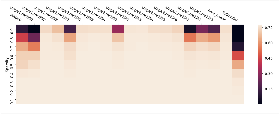](https://mlsysbook.ai/contents/core/optimizations/images/png/sprase-heat-map_a50fe5a9.png "Figure 32: Sparsity Distribution: Pruned neural networks exhibit varying degrees of weight removal across layers; darker shades indicate higher sparsity, revealing which parts of the model were most affected by the pruning process. Analyzing this distribution helps practitioners understand and refine sparsity-aware optimization strategies for model compression and efficiency. Source: numenta")
Figure 32: **Sparsity Distribution**: Pruned neural networks exhibit varying degrees of weight removal across layers; darker shades indicate higher sparsity, revealing which parts of the model were most affected by the pruning process. Analyzing this distribution helps practitioners understand and refine sparsity-aware optimization strategies for model compression and efficiency. Source: [numenta](https://www.numenta.com/blog/)
Beyond static snapshots, trend plots track sparsity progression across multiple pruning iterations. These visualizations illustrate how global model sparsity evolves, often showing an initial rapid increase followed by more gradual refinements. Tools like TensorFlow’s Model Optimization Toolkit and SparseML’s monitoring utilities provide such tracking capabilities, displaying per-layer pruning levels over time. These insights allow practitioners to fine-tune pruning strategies by adjusting sparsity constraints for individual layers.
Libraries such as DeepSparse’s visualization suite and PyTorch’s pruning utilities enable the generation of these visualization tools, helping analyze how pruning decisions affect different model components. By making sparsity data visually accessible, these tools help practitioners optimize their models more effectively.
**Self-Check: Question 1.11**
1. Which of the following best describes the role of modern machine learning frameworks in model optimization?
1. They provide theoretical insights into optimization techniques.
2. They replace the need for model optimization entirely.
3. They automate the implementation of complex optimization algorithms.
4. They focus solely on hardware-specific optimizations.
2. Explain how built-in optimization APIs in frameworks like TensorFlow and PyTorch enhance model efficiency.
3. True or False: Visualization tools are unnecessary in understanding the impact of model optimization techniques like pruning and quantization.
4. In machine learning frameworks, the process of reducing numerical precision to improve computational efficiency is known as \_\_\_\_. This process involves converting models to lower-precision formats while maintaining accuracy.
5. In a production system, what trade-offs might you consider when choosing between different optimization techniques provided by software frameworks?
[See Answers →](https://mlsysbook.ai/contents/core/optimizations/optimizations.html#quiz-answer-sec-model-optimizations-implementation-tools-software-frameworks-5681)
Technique Comparison
--------------------
Having explored the three major optimization approaches in depth, a comparative analysis reveals how different techniques address distinct aspects of the efficiency-accuracy trade-off. This comparison guides technique selection based on deployment constraints and available resources.
Table 12: **Optimization Technique Trade-offs**: Comparison of the three major optimization approaches across key performance dimensions, highlighting how each technique addresses different constraints and deployment scenarios. Pruning excels for computational reduction but requires sparse hardware support, quantization provides balanced size and speed improvements with wide hardware compatibility, while distillation produces high-quality compressed models at higher training cost.
| | | | | | |
| --- | --- | --- | --- | --- | --- |
| **Pruning** | Reduce FLOPs/Size | Moderate | Low (fine-tuning) | High (for sparse ops) | Latency-critical apps |
| **Quantization** | Reduce Size/Latency | Low | Low (PTQ) / High (QAT) | High (INT8 support) | Edge/Mobile deployment |
| **Distillation** | Reduce Size | Low-Moderate | High (retraining) | Low | Creating smaller, high-quality models |
Understanding these trade-offs enables systematic technique selection ([Table 12](https://mlsysbook.ai/contents/core/optimizations/optimizations.html#tbl-optimization-comparison)
). Pruning works best when sparse computation hardware is available and when reducing floating-point operations is critical. Quantization provides the most versatile approach with broad hardware support, making it ideal for diverse deployment scenarios. Knowledge distillation requires significant computational investment but produces consistently high-quality compressed models, making it valuable when accuracy preservation is paramount.
These techniques combine synergistically, with quantization often applied after pruning or distillation to achieve compound compression benefits. Production systems frequently employ sequential application: initial pruning reduces parameter count, quantization optimizes numerical representation, and fine-tuning through distillation principles recovers any accuracy loss. Sequential application enables compression ratios of 10-50x while maintaining competitive accuracy across diverse deployment scenarios.
**Self-Check: Question 1.12**
1. Which optimization technique is best suited for latency-critical applications where sparse computation hardware is available?
1. Pruning
2. Quantization
3. Distillation
4. All of the above
2. True or False: Quantization is the most versatile optimization technique due to its broad hardware support.
3. Explain why knowledge distillation might be preferred when accuracy preservation is paramount in a production system.
4. Order the following optimization techniques based on their typical application sequence in a production system: (1) Pruning, (2) Quantization, (3) Distillation.
[See Answers →](https://mlsysbook.ai/contents/core/optimizations/optimizations.html#quiz-answer-sec-model-optimizations-technique-comparison-5bec)
Fallacies and Pitfalls
----------------------
Model optimization represents one of the most technically complex areas in machine learning systems, where multiple techniques must be coordinated to achieve efficiency gains without sacrificing accuracy. The sophisticated nature of pruning, quantization, and distillation techniques—combined with their complex interdependencies—creates numerous opportunities for misapplication and suboptimal results that can undermine deployment success.
**Fallacy:** _Optimization techniques can be applied independently without considering their interactions._
This misconception leads teams to apply multiple optimization techniques simultaneously without understanding how they interact. Combining pruning with aggressive quantization might compound accuracy losses beyond acceptable levels, while knowledge distillation from heavily pruned models may transfer suboptimal behaviors to student networks. Different optimization approaches can interfere with each other’s effectiveness, creating complex trade-offs that require careful orchestration. Successful optimization requires understanding technique interactions and applying them in coordinated strategies rather than as independent modifications.
**Pitfall:** _Optimizing for theoretical metrics rather than actual deployment performance._
Many practitioners focus on reducing parameter counts, FLOPs, or model size without measuring actual deployment performance improvements. A model with fewer parameters might still have poor cache locality, irregular memory access patterns, or inefficient hardware utilization that negates theoretical efficiency gains. Quantization that reduces model size might increase inference latency on certain hardware platforms due to format conversion overhead. Effective optimization requires measuring and optimizing for actual deployment metrics rather than relying on theoretical complexity reductions.
**Fallacy:** _Aggressive quantization maintains model performance with minimal accuracy loss._
This belief drives teams to apply extreme quantization levels without understanding the relationship between numerical precision and model expressiveness. While many models tolerate moderate quantization well, extreme quantization can cause catastrophic accuracy degradation, numerical instability, or training divergence. Different model architectures and tasks have varying sensitivity to quantization, requiring careful analysis rather than assuming universal applicability. Some operations like attention mechanisms or normalization layers may require higher precision to maintain functionality.
**Pitfall:** _Using post-training optimization without considering training-aware alternatives._
Teams often apply optimization techniques after training completion to avoid modifying existing training pipelines. Post-training optimization is convenient but typically achieves inferior results compared to optimization-aware training approaches. Quantization-aware training, gradual pruning during training, and distillation-integrated training can achieve better accuracy-efficiency trade-offs than applying these techniques post-hoc. The convenience of post-training optimization comes at the cost of suboptimal results that may not meet deployment requirements.
**Pitfall:** _Focusing on individual model optimization without considering system-level performance bottlenecks._
Many optimization efforts concentrate solely on reducing model complexity without analyzing the broader system context where models operate, requiring the structured profiling approaches detailed in **[Chapter 12: Benchmarking AI](https://mlsysbook.ai/contents/core/benchmarking/benchmarking.html#sec-benchmarking-ai)
**. A highly optimized model may provide minimal benefit if data preprocessing pipelines, I/O operations, or network communication dominate overall system latency. Memory bandwidth limitations, cache misses, or inefficient batch processing can negate the advantages of aggressive model optimization. Similarly, optimizing for single-model inference may miss opportunities for throughput improvements through batch processing, model parallelism, or request pipelining. Effective optimization requires profiling the entire system to identify actual bottlenecks and ensuring that model-level improvements translate to measurable system-level performance gains. This systems perspective is particularly important in multi-model ensembles, real-time serving systems, or edge deployments where resource constraints extend beyond individual model efficiency. The holistic optimization approach connects directly to the operational excellence principles **[Chapter 13: ML Operations](https://mlsysbook.ai/contents/core/ops/ops.html#sec-ml-operations)
** by ensuring that optimizations contribute to overall system reliability and maintainability.
**Self-Check: Question 1.13**
1. True or False: Optimization techniques like pruning and quantization can be applied independently without considering their interactions.
2. Which of the following is a potential pitfall when optimizing machine learning models?
1. Profiling the entire system for bottlenecks
2. Measuring actual deployment performance
3. Applying optimization-aware training
4. Focusing solely on reducing parameter counts
3. Explain why aggressive quantization might not always maintain model performance.
4. What is a disadvantage of using post-training optimization techniques?
1. They require modification of existing training pipelines
2. They are more complex to implement than training-aware techniques
3. They typically achieve inferior results compared to training-aware approaches
4. They always result in higher inference latency
5. In a production system, why is it important to consider system-level performance bottlenecks when optimizing models?
[See Answers →](https://mlsysbook.ai/contents/core/optimizations/optimizations.html#quiz-answer-sec-model-optimizations-fallacies-pitfalls-97f2)
Summary
-------
Model optimization represents the important bridge between theoretical machine learning advances and practical deployment realities, where computational constraints, memory limitations, and energy efficiency requirements demand sophisticated engineering solutions. This chapter demonstrated how the core tension between model accuracy and resource efficiency drives a rich ecosystem of optimization techniques that operate across multiple dimensions simultaneously. Rather than simply reducing model size or complexity, modern optimization approaches strategically reorganize model representations, numerical precision, and computational patterns to preserve important capabilities while dramatically improving efficiency characteristics.
Our optimization framework demonstrates how different aspects of model design can be systematically refined to meet deployment constraints. The journey from a 440MB BERT-Base model ([Devlin et al. 2018](https://mlsysbook.ai/contents/core/optimizations/optimizations.html#ref-devlin2018bert)
) to a 28MB deployment-ready version exemplifies the power of combining complementary techniques: structural pruning shrinks the model to 110MB, knowledge distillation with DistilBERT ([Sanh et al. 2019](https://mlsysbook.ai/contents/core/optimizations/optimizations.html#ref-sanh2019distilbert)
) maintains performance while further reducing size, and INT8 quantization achieves the final 28MB target. The integration of hardware-aware design principles ensures that optimization strategies align with underlying computational architectures, maximizing practical benefits across different deployment environments.
Devlin, Jacob, Ming-Wei Chang, Kenton Lee, and Kristina Toutanova. 2018. “BERT: Pre-Training of Deep Bidirectional Transformers for Language Understanding.” _arXiv Preprint arXiv:1810.04805_, October. [http://arxiv.org/abs/1810.04805v2](http://arxiv.org/abs/1810.04805v2)
.
Sanh, Victor, Lysandre Debut, Julien Chaumond, and Thomas Wolf. 2019. “DistilBERT, a Distilled Version of BERT: Smaller, Faster, Cheaper and Lighter.” _arXiv Preprint arXiv:1910.01108_, October. [http://arxiv.org/abs/1910.01108v4](http://arxiv.org/abs/1910.01108v4)
.
Key Takeaways
* Model optimization requires coordinated approaches across representation, precision, and architectural efficiency—as demonstrated by BERT’s 16x compression through combined pruning, distillation, and quantization
* Hardware-aware optimization aligns model characteristics with computational architectures to maximize practical performance benefits
* Automated optimization through AutoML can discover novel combinations of techniques that outperform manual optimization strategies
* Optimization techniques must balance accuracy preservation with deployment constraints—DistilBERT retains 97% of BERT’s performance with 40% fewer parameters
* Success requires understanding that no single technique provides a universal solution; the optimal strategy depends on specific deployment constraints, hardware characteristics, and application requirements
The emergence of AutoML frameworks for optimization represents a paradigm shift toward automated discovery of optimization strategies that can adapt to specific deployment contexts and performance requirements. These automated approaches build on training methodologies while pointing toward the emerging frontiers of self-optimizing systems. Such systems enable practitioners to explore vast optimization spaces more systematically than manual approaches, often uncovering novel combinations of techniques that achieve superior efficiency-accuracy trade-offs. As models grow larger and deployment contexts become more diverse, mastering these optimization techniques becomes increasingly critical for bridging the gap between research accuracy and production efficiency.
**Self-Check: Question 1.14**
1. Which of the following best illustrates the trade-off between model accuracy and resource efficiency in optimization?
1. Increasing model size to improve accuracy
2. Applying structural pruning to reduce model size
3. Using more complex algorithms without considering deployment
4. Focusing solely on reducing computational time
2. Explain how combining structural pruning, knowledge distillation, and quantization can achieve significant model size reduction while maintaining performance.
3. True or False: AutoML frameworks can discover optimization strategies that outperform manual methods by exploring vast optimization spaces.
4. The process of reducing numerical precision to improve computational efficiency is known as \_\_\_\_. This technique helps in minimizing model size and computational load.
5. In a production system, what trade-offs might you consider when implementing hardware-aware optimization strategies?
[See Answers →](https://mlsysbook.ai/contents/core/optimizations/optimizations.html#quiz-answer-sec-model-optimizations-summary-98df)
Self-Check Answers
------------------
**Self-Check: Answer 1.1**
1. **Which of the following best describes the primary goal of model optimization in machine learning systems?**
1. Maximize model accuracy regardless of resource constraints.
2. Reduce the size of the model to the smallest possible footprint.
3. Achieve efficient execution in target environments while maintaining accuracy and functionality.
4. Increase the complexity of the model to improve performance.
_Answer_: The correct answer is C. Achieve efficient execution in target environments while maintaining accuracy and functionality. This is correct because model optimization focuses on balancing efficiency with performance across various constraints.
_Learning Objective_: Understand the primary goal of model optimization in ML systems.
2. **Explain how model optimization techniques like quantization and pruning contribute to efficient deployment of machine learning models.**
_Answer_: Quantization reduces memory usage and speeds up inference by using lower precision data types. Pruning removes redundant parameters, maintaining model accuracy while reducing computational load. These techniques enable deployment in resource-constrained environments by optimizing resource utilization.
_Learning Objective_: Describe how specific optimization techniques improve model deployment efficiency.
3. **What is a common challenge when deploying sophisticated machine learning models on mobile devices?**
1. Excessive computational throughput
2. Unlimited thermal constraints
3. High latency requirements
4. Limited memory and energy resources
_Answer_: The correct answer is D. Limited memory and energy resources. Mobile devices often have limited memory and battery life, making it challenging to deploy large, sophisticated models without optimization.
_Learning Objective_: Identify challenges associated with deploying ML models on resource-constrained devices.
4. **True or False: Model optimization only focuses on reducing the computational complexity of machine learning models.**
_Answer_: False. Model optimization also addresses memory utilization, inference latency, and energy efficiency, balancing multiple performance objectives.
_Learning Objective_: Recognize the multi-faceted nature of model optimization beyond computational complexity.
5. **In a production system, what trade-offs might you consider when implementing model optimization techniques?**
_Answer_: Consider trade-offs between model accuracy and resource usage, such as memory and energy consumption. Balancing these can affect performance metrics like latency and throughput, impacting user experience and operational costs.
_Learning Objective_: Analyze trade-offs involved in applying model optimization techniques in production systems.
[← Back to Questions](https://mlsysbook.ai/contents/core/optimizations/optimizations.html#quiz-question-sec-model-optimizations-model-optimization-fundamentals-064e)
**Self-Check: Answer 1.2**
1. **Which of the following layers in the optimization stack primarily focuses on aligning computation patterns with processor designs?**
1. Efficient Model Representation
2. Efficient Numerics Representation
3. Efficient Data Handling
4. Efficient Hardware Implementation
_Answer_: The correct answer is D. Efficient Hardware Implementation. This layer focuses on aligning computation patterns with processor designs to enhance execution efficiency. Other options address different aspects of optimization.
_Learning Objective_: Understand the role of efficient hardware implementation in the optimization stack.
2. **Explain how model representation techniques such as pruning and distillation can create opportunities for numerical precision optimization.**
_Answer_: Model representation techniques like pruning and distillation reduce computational complexity, which allows for numerical precision optimization by freeing up resources. For example, pruning reduces model size, enabling the use of quantization techniques that exploit hardware capabilities for faster execution. This is important because it enhances model efficiency while maintaining performance.
_Learning Objective_: Analyze the interaction between model representation techniques and numerical precision optimization.
3. **In the context of the optimization framework, what is the primary benefit of using quantization techniques?**
1. Increasing model accuracy
2. Reducing computational cost
3. Enhancing data privacy
4. Improving data collection
_Answer_: The correct answer is B. Reducing computational cost. Quantization techniques primarily reduce computational cost by using reduced-precision arithmetic, which exploits hardware capabilities for faster execution. Other options do not directly relate to the primary benefit of quantization.
_Learning Objective_: Understand the primary benefit of quantization techniques in the optimization framework.
4. **True or False: The optimization framework’s effectiveness is independent of the target hardware characteristics.**
_Answer_: False. The effectiveness of the optimization framework depends on the target hardware characteristics, as the techniques must align with the hardware’s capabilities to maximize performance and efficiency.
_Learning Objective_: Recognize the dependency of optimization effectiveness on hardware characteristics.
[← Back to Questions](https://mlsysbook.ai/contents/core/optimizations/optimizations.html#quiz-question-sec-model-optimizations-optimization-framework-1c8e)
**Self-Check: Answer 1.3**
1. **Which of the following is a primary constraint when deploying machine learning models on microcontrollers?**
1. High memory bandwidth
2. Limited computational resources
3. Large storage capacity
4. Unlimited power supply
_Answer_: The correct answer is B. Limited computational resources. Microcontrollers have limited computational power and memory, which constrain the complexity of models that can be deployed.
_Learning Objective_: Understand the constraints specific to deploying ML models on microcontrollers.
2. **True or False: In cloud environments, optimizing machine learning models primarily focuses on reducing the model’s memory footprint.**
_Answer_: False. In cloud environments, optimization focuses on minimizing training time, computational cost, and power consumption, not just memory footprint.
_Learning Objective_: Recognize the primary optimization goals in different deployment contexts.
3. **Explain why balancing accuracy and efficiency is crucial when deploying machine learning models on edge devices.**
_Answer_: Balancing accuracy and efficiency is crucial on edge devices because these devices have limited computational resources and must process data locally to reduce latency. For example, a highly accurate model that is too resource-intensive cannot run effectively on a smartphone. This balance ensures real-time responsiveness while maintaining acceptable performance.
_Learning Objective_: Analyze the trade-offs between accuracy and efficiency in edge ML deployments.
4. **In the context of deployment, the term ‘\_\_\_\_’ refers to the computational paradigm where ML inference occurs on local devices rather than cloud servers.**
_Answer_: Edge ML. Edge ML refers to performing machine learning inference on local devices, reducing latency and dependency on cloud resources.
_Learning Objective_: Recall specific terminology related to deployment contexts.
5. **In a production system, how might you address the trade-off between model complexity and energy efficiency?**
_Answer_: In a production system, addressing the trade-off between model complexity and energy efficiency might involve techniques such as model pruning, quantization, or using more efficient algorithms. For example, pruning can reduce the number of parameters, lowering energy consumption while maintaining acceptable accuracy. This is important to ensure the model operates effectively within the energy constraints of the deployment environment.
_Learning Objective_: Evaluate strategies for balancing model complexity with energy efficiency in practical deployments.
[← Back to Questions](https://mlsysbook.ai/contents/core/optimizations/optimizations.html#quiz-question-sec-model-optimizations-deployment-context-c1b0)
**Self-Check: Answer 1.4**
1. **Which optimization dimension should be prioritized when addressing memory and storage constraints?**
1. Architectural Efficiency only
2. Numerical Precision and Architectural Efficiency
3. Model Representation and Architectural Efficiency
4. Model Representation and Numerical Precision
_Answer_: The correct answer is D. Model Representation and Numerical Precision. These dimensions help reduce parameter count and bit-width, addressing memory and storage constraints effectively.
_Learning Objective_: Understand how specific system constraints map to optimization dimensions.
2. **True or False: Inference latency requirements are best addressed by focusing solely on numerical precision techniques.**
_Answer_: False. Inference latency is best addressed by focusing on model representation and architectural efficiency, which reduce computational workload and improve hardware utilization.
_Learning Objective_: Identify the appropriate optimization strategies for specific system constraints.
3. **Explain why system-wide profiling is essential before investing in model optimization.**
_Answer_: System-wide profiling identifies bottlenecks that may limit the effectiveness of model optimization. For example, if data preprocessing or network I/O dominate latency, model optimization may have minimal impact. This is important because it ensures optimization efforts are targeted and effective.
_Learning Objective_: Understand the importance of system-level analysis in the optimization process.
4. **Order the following optimization strategies based on their typical application sequence in production systems: (1) Quantization, (2) Reducing Parameters, (3) Training Refinement.**
_Answer_: The correct order is: (2) Reducing Parameters, (3) Training Refinement, (1) Quantization. This sequence achieves compression and accuracy recovery before applying final quantization for deployment.
_Learning Objective_: Recognize the typical sequence of optimization strategies in production systems.
[← Back to Questions](https://mlsysbook.ai/contents/core/optimizations/optimizations.html#quiz-question-sec-model-optimizations-framework-application-navigation-03d4)
**Self-Check: Answer 1.5**
1. **Which optimization dimension primarily focuses on reducing the redundancy in the structure of machine learning models?**
1. Architectural Efficiency Optimization
2. Numerical Precision Optimization
3. Model Representation Optimization
4. Operational Scheduling Optimization
_Answer_: The correct answer is C. Model Representation Optimization. This dimension focuses on eliminating unnecessary parameters and components in models to enhance efficiency. The other options address different aspects of optimization.
_Learning Objective_: Understand the primary focus of model representation optimization.
2. **Explain how numerical precision optimization can impact the execution efficiency of machine learning models on hardware accelerators.**
_Answer_: Numerical precision optimization reduces the bit-width of weights and activations, allowing models to execute more efficiently on hardware accelerators like GPUs and TPUs. For example, quantization maps high-precision values to lower-bit representations, reducing computational load and memory usage. This is important because it enables faster execution and lower power consumption in resource-constrained environments.
_Learning Objective_: Analyze the impact of numerical precision optimization on hardware efficiency.
3. **What is a key benefit of architectural efficiency optimization in machine learning models?**
1. Reduced inference latency
2. Increased model accuracy
3. Higher memory usage
4. Greater model complexity
_Answer_: The correct answer is A. Reduced inference latency. Architectural efficiency optimization techniques, such as exploiting sparsity, help reduce the computational demands and improve execution speed, thus lowering latency. The other options do not align with the primary benefits of architectural efficiency.
_Learning Objective_: Identify the benefits of architectural efficiency optimization.
4. **In a production system with strict memory constraints, how would you apply the three-dimensional optimization framework to deploy an efficient machine learning model?**
_Answer_: In a memory-constrained production system, I would apply model representation optimization to reduce the model size through pruning and architecture search. Numerical precision optimization would be used to lower the bit-width of weights and activations, reducing memory usage. Finally, architectural efficiency techniques like exploiting sparsity would minimize computational overhead. This holistic approach ensures the model is both efficient and effective within the given constraints.
_Learning Objective_: Apply the three-dimensional optimization framework to address specific system constraints.
[← Back to Questions](https://mlsysbook.ai/contents/core/optimizations/optimizations.html#quiz-question-sec-model-optimizations-optimization-dimensions-e571)
**Self-Check: Answer 1.6**
1. **Which of the following best describes the purpose of gradient checkpointing in neural network optimization?**
1. To reduce memory usage by recomputing intermediate activations during backpropagation.
2. To improve model accuracy by increasing the number of parameters.
3. To enhance computational speed by parallelizing model training.
4. To eliminate redundant parameters through pruning.
_Answer_: The correct answer is A. To reduce memory usage by recomputing intermediate activations during backpropagation. Gradient checkpointing trades computation for memory, allowing larger models or batch sizes to fit into the same GPU memory.
_Learning Objective_: Understand the role of gradient checkpointing in optimizing memory usage during model training.
2. **Explain the trade-offs involved in model pruning and how it affects deployment in different environments.**
_Answer_: Pruning reduces model size by removing redundant parameters, improving memory and computational efficiency. However, aggressive pruning can degrade accuracy, making models unreliable for production. In cloud environments, pruning helps scale models efficiently, while on edge devices, it ensures models fit within resource constraints. Balancing pruning extent is crucial to maintain performance across diverse deployment scenarios.
_Learning Objective_: Analyze the trade-offs of model pruning in various deployment environments.
3. **The process of systematically removing redundant parameters from a neural network while preserving accuracy is known as \_\_\_\_. This technique reduces model size and computational cost.**
_Answer_: pruning. Pruning eliminates unnecessary parameters, making models more efficient for storage, inference, and deployment.
_Learning Objective_: Recall the definition and purpose of pruning in neural network optimization.
4. **What is a primary advantage of using parallel processing patterns in machine learning model optimization?**
1. It increases the number of parameters in the model.
2. It reduces the need for gradient checkpointing.
3. It allows for faster training by utilizing multiple cores simultaneously.
4. It eliminates the need for model pruning.
_Answer_: The correct answer is C. It allows for faster training by utilizing multiple cores simultaneously. Parallel processing leverages high core counts in GPUs to speed up model training and inference.
_Learning Objective_: Understand the benefits of parallel processing in accelerating model training and deployment.
[← Back to Questions](https://mlsysbook.ai/contents/core/optimizations/optimizations.html#quiz-question-sec-model-optimizations-structural-model-optimization-methods-ca9e)
**Self-Check: Answer 1.7**
1. **Which of the following precision formats offers the best balance between computational speed and accuracy for training on AI accelerators?**
1. BFloat16
2. FP16
3. INT8
4. FP32
_Answer_: The correct answer is A. BFloat16. BFloat16 retains the same exponent size as FP32, allowing it to maintain a wider dynamic range while reducing precision in the fraction, making it effective for training on AI accelerators.
_Learning Objective_: Understand the balance between computational speed and accuracy provided by different precision formats.
2. **Explain the trade-offs involved in using INT8 precision for inference in machine learning models.**
_Answer_: Using INT8 precision significantly reduces storage and computational requirements, leading to faster inference and lower power consumption. However, it may introduce quantization noise and accuracy degradation, especially in models sensitive to precision loss. Balancing these trade-offs involves ensuring hardware support and employing techniques like quantization-aware training to mitigate accuracy loss.
_Learning Objective_: Analyze the trade-offs of using INT8 precision in terms of efficiency and accuracy.
3. **The process of reducing numerical precision to improve computational efficiency is known as \_\_\_\_. This technique is essential for optimizing machine learning models for deployment in resource-constrained environments.**
_Answer_: quantization. Quantization reduces the bit-width of numerical representations, enhancing computational efficiency and reducing power consumption, particularly in resource-constrained environments.
_Learning Objective_: Recall the term used for reducing numerical precision to enhance computational efficiency.
4. **True or False: Reducing precision from FP32 to FP16 always leads to a proportional decrease in power consumption.**
_Answer_: False. While reducing precision from FP32 to FP16 can lead to significant power savings, the relationship is not always proportional due to factors such as hardware support and the need for additional techniques to manage quantization errors.
_Learning Objective_: Understand the non-linear relationship between precision reduction and power consumption.
5. **Order the following precision formats by their typical storage reduction compared to FP32: (1) FP16, (2) INT8, (3) BFloat16.**
_Answer_: The correct order is: (2) INT8, (1) FP16, (3) BFloat16. INT8 offers the most significant storage reduction, followed by FP16, and then BFloat16, which maintains a larger exponent for dynamic range.
_Learning Objective_: Sequence precision formats based on their storage efficiency compared to FP32.
[← Back to Questions](https://mlsysbook.ai/contents/core/optimizations/optimizations.html#quiz-question-sec-model-optimizations-quantization-precision-optimization-e90a)
**Self-Check: Answer 1.8**
1. **Which of the following best describes the goal of architectural efficiency optimization in machine learning systems?**
1. Aligning model operations with hardware capabilities
2. Improving numerical precision of computations
3. Increasing the number of model parameters
4. Enhancing the theoretical accuracy of models
_Answer_: The correct answer is A. Aligning model operations with hardware capabilities. This is correct because architectural efficiency focuses on optimizing how operations are scheduled and executed on specific hardware, rather than altering the computations themselves. Other options do not address the system-level optimization focus of architectural efficiency.
_Learning Objective_: Understand the primary goal of architectural efficiency optimization in ML systems.
2. **Explain how hardware-aware design principles can improve the deployment efficiency of machine learning models.**
_Answer_: Hardware-aware design principles improve deployment efficiency by ensuring that model architectures are tailored to the specific capabilities and constraints of the target hardware. This includes optimizing for memory bandwidth, processing power, and parallelism, which reduces latency and increases throughput. For example, using depthwise separable convolutions on mobile chips can significantly reduce computational cost while maintaining performance. This is important because it allows models to be efficiently deployed across diverse hardware environments.
_Learning Objective_: Analyze the impact of hardware-aware design principles on model deployment efficiency.
3. **Which architectural efficiency technique involves reducing memory traffic by combining operations?**
1. Dynamic computation strategies
2. Sparsity exploitation techniques
3. Operator fusion methods
4. Hardware-aware design
_Answer_: The correct answer is C. Operator fusion methods. This is correct because operator fusion reduces memory traffic by combining multiple operations into a single operation, thereby minimizing the need for intermediate data storage and transfer. Other options focus on different aspects of architectural efficiency.
_Learning Objective_: Identify techniques that reduce memory traffic in ML systems.
4. **In a production system, what trade-offs would you consider when implementing dynamic computation strategies?**
_Answer_: When implementing dynamic computation strategies, trade-offs include balancing computational efficiency with predictive performance. These strategies allow models to adapt computational load based on input complexity, which can reduce energy consumption and latency. However, this may introduce variability in inference time and require additional control mechanisms, potentially complicating deployment. For example, in real-time applications, ensuring consistent latency while maintaining accuracy is crucial. This is important because it affects the system’s ability to meet performance requirements under varying conditions.
_Learning Objective_: Evaluate trade-offs involved in implementing dynamic computation strategies in production systems.
[← Back to Questions](https://mlsysbook.ai/contents/core/optimizations/optimizations.html#quiz-question-sec-model-optimizations-architectural-efficiency-techniques-ba84)
**Self-Check: Answer 1.9**
1. **Which of the following is a critical first step in the optimization process for machine learning systems?**
1. Applying quantization to reduce model size
2. Conducting sensitivity analysis on model parameters
3. Implementing structured pruning techniques
4. Establishing baseline measurements through profiling
_Answer_: The correct answer is D. Establishing baseline measurements through profiling. This is correct because profiling identifies where resources are consumed and which components offer optimization potential. Other options are specific techniques applied after profiling.
_Learning Objective_: Understand the importance of profiling as the foundational step in optimization.
2. **True or False: In a production environment, model computation often represents the majority of system overhead.**
_Answer_: False. This is false because model computation typically represents only a fraction of total system overhead, highlighting the importance of profiling to identify optimization opportunities.
_Learning Objective_: Challenge the misconception about the role of model computation in system overhead.
3. **Explain how a systematic measurement framework can help balance competing optimization objectives in ML systems.**
_Answer_: A systematic measurement framework helps balance competing objectives by establishing clear baselines across multiple metrics, such as accuracy, computational efficiency, and energy consumption. For example, quantizing a model may reduce latency but affect accuracy, so a framework ensures trade-offs are evaluated comprehensively. This is important because it guides informed decision-making in optimization.
_Learning Objective_: Understand the role of measurement frameworks in balancing optimization objectives.
4. **Order the following stages of deploying BERT-Base on mobile devices: (1) Quantization-aware training, (2) Structured pruning, (3) Knowledge distillation.**
_Answer_: The correct order is: (2) Structured pruning, (3) Knowledge distillation, (1) Quantization-aware training. Pruning first concentrates important weights, making subsequent quantization more effective. Knowledge distillation helps recover accuracy before final quantization.
_Learning Objective_: Understand the importance of sequencing in multi-technique optimization strategies.
5. **In a production system, what trade-offs would you consider when integrating multiple optimization techniques?**
_Answer_: When integrating multiple optimization techniques, consider trade-offs between accuracy, computational efficiency, and resource consumption. For instance, pruning may reduce model size but affect accuracy, while quantization reduces computational cost but may impact precision. Balancing these requires understanding dependencies and sequencing techniques to maximize cumulative benefits. This is important because it ensures that optimizations do not introduce conflicts or diminish returns.
_Learning Objective_: Evaluate trade-offs in integrating multiple optimization techniques in production systems.
[← Back to Questions](https://mlsysbook.ai/contents/core/optimizations/optimizations.html#quiz-question-sec-model-optimizations-implementation-strategy-evaluation-a052)
**Self-Check: Answer 1.10**
1. **Which of the following best describes the role of AutoML in machine learning model optimization?**
1. It completely replaces the need for human expertise in model design.
2. It automates the search for optimal model configurations, reducing manual effort.
3. It focuses solely on improving model accuracy without considering efficiency.
4. It is primarily used for data collection and preprocessing.
_Answer_: The correct answer is B. It automates the search for optimal model configurations, reducing manual effort. AutoML enhances human expertise by providing a structured approach to optimization, balancing accuracy and efficiency.
_Learning Objective_: Understand the primary function and benefits of AutoML in the context of model optimization.
2. **Explain how AutoML frameworks balance accuracy and efficiency in model optimization.**
_Answer_: AutoML frameworks employ techniques like neural architecture search and hyperparameter optimization to explore a vast design space, selecting configurations that meet predefined accuracy and efficiency objectives. This structured approach allows for the discovery of novel solutions that balance these factors effectively.
_Learning Objective_: Analyze the methods AutoML uses to optimize machine learning models while balancing multiple objectives.
3. **True or False: AutoML can fully eliminate the need for domain expertise in model optimization.**
_Answer_: False. AutoML enhances but does not replace domain expertise. It provides a structured approach to optimization, allowing experts to focus on high-level objectives while automating routine tasks.
_Learning Objective_: Challenge misconceptions about the role of AutoML in replacing human expertise.
4. **The process of automatically selecting pruning thresholds and quantization levels in AutoML is known as \_\_\_\_.**
_Answer_: model compression. This process reduces the memory footprint and computational requirements of a model, making it suitable for deployment on resource-constrained hardware.
_Learning Objective_: Recall specific optimization techniques used in AutoML for efficient model deployment.
5. **In a production system, what trade-offs might you consider when implementing AutoML for model optimization?**
_Answer_: Consider trade-offs between computational cost and optimization quality. AutoML requires significant computational resources, but can yield highly optimized models. Balancing these factors involves assessing the available infrastructure and the importance of achieving optimal performance versus resource expenditure.
_Learning Objective_: Evaluate the practical considerations and trade-offs involved in deploying AutoML in real-world systems.
[← Back to Questions](https://mlsysbook.ai/contents/core/optimizations/optimizations.html#quiz-question-sec-model-optimizations-automl-automated-optimization-strategies-329f)
**Self-Check: Answer 1.11**
1. **Which of the following best describes the role of modern machine learning frameworks in model optimization?**
1. They provide theoretical insights into optimization techniques.
2. They replace the need for model optimization entirely.
3. They automate the implementation of complex optimization algorithms.
4. They focus solely on hardware-specific optimizations.
_Answer_: The correct answer is C. They automate the implementation of complex optimization algorithms. This is correct because modern frameworks offer high-level APIs and automated workflows that simplify the application of optimization techniques. Option A is incorrect as frameworks focus on practical implementation, not theoretical insights. Option A is incorrect as frameworks assist but do not replace optimization. Option D is incorrect as frameworks address a broader range of optimization challenges.
_Learning Objective_: Understand the role of machine learning frameworks in simplifying the implementation of optimization techniques.
2. **Explain how built-in optimization APIs in frameworks like TensorFlow and PyTorch enhance model efficiency.**
_Answer_: Built-in optimization APIs provide pre-tested modules for techniques like quantization and pruning, reducing the need for manual implementation. For example, TensorFlow’s Model Optimization Toolkit facilitates quantization by converting models to lower-precision formats while preserving accuracy. This is important because it enables practitioners to apply complex optimizations reliably and consistently across different architectures.
_Learning Objective_: Explain the benefits of using built-in optimization APIs for enhancing model efficiency.
3. **True or False: Visualization tools are unnecessary in understanding the impact of model optimization techniques like pruning and quantization.**
_Answer_: False. Visualization tools are essential for understanding the impact of optimization techniques. They provide insights into sparsity patterns and quantization errors, helping practitioners diagnose and mitigate issues. For example, quantization error histograms reveal error distributions, guiding adjustments to maintain model accuracy.
_Learning Objective_: Recognize the importance of visualization tools in interpreting the effects of optimization techniques.
4. **In machine learning frameworks, the process of reducing numerical precision to improve computational efficiency is known as \_\_\_\_. This process involves converting models to lower-precision formats while maintaining accuracy.**
_Answer_: quantization. This process involves converting models to lower-precision formats while maintaining accuracy.
_Learning Objective_: Recall the term for reducing numerical precision in model optimization.
5. **In a production system, what trade-offs might you consider when choosing between different optimization techniques provided by software frameworks?**
_Answer_: When choosing optimization techniques, consider trade-offs between model accuracy and computational efficiency. For example, quantization can reduce precision and computational load but may introduce rounding errors affecting accuracy. Pruning reduces model size but may impact performance if not carefully managed. Balancing these factors is crucial for optimal deployment.
_Learning Objective_: Evaluate trade-offs in selecting optimization techniques for production systems.
[← Back to Questions](https://mlsysbook.ai/contents/core/optimizations/optimizations.html#quiz-question-sec-model-optimizations-implementation-tools-software-frameworks-5681)
**Self-Check: Answer 1.12**
1. **Which optimization technique is best suited for latency-critical applications where sparse computation hardware is available?**
1. Pruning
2. Quantization
3. Distillation
4. All of the above
_Answer_: The correct answer is A. Pruning. This is correct because pruning reduces floating-point operations and is most effective when sparse computation hardware is available. Quantization and distillation do not specifically target latency-critical applications in the same way.
_Learning Objective_: Understand the specific use cases and hardware dependencies of different optimization techniques.
2. **True or False: Quantization is the most versatile optimization technique due to its broad hardware support.**
_Answer_: True. This is true because quantization can be applied to a wide range of hardware platforms, making it ideal for diverse deployment scenarios.
_Learning Objective_: Recognize the versatility and hardware compatibility of quantization as an optimization technique.
3. **Explain why knowledge distillation might be preferred when accuracy preservation is paramount in a production system.**
_Answer_: Knowledge distillation is preferred when accuracy preservation is paramount because it produces high-quality compressed models. For example, in scenarios where model size needs to be reduced without significant loss of accuracy, distillation can provide a balance between compression and performance. This is important because maintaining model accuracy is crucial in applications where precision is critical.
_Learning Objective_: Analyze the trade-offs involved in using knowledge distillation for accuracy-sensitive applications.
4. **Order the following optimization techniques based on their typical application sequence in a production system: (1) Pruning, (2) Quantization, (3) Distillation.**
_Answer_: The correct order is: (1) Pruning, (3) Distillation, (2) Quantization. Pruning is typically applied first to reduce the parameter count, distillation is used to recover accuracy, and quantization is applied last to optimize numerical representation. This sequence maximizes compression while maintaining accuracy.
_Learning Objective_: Understand the sequential application of optimization techniques in production systems.
[← Back to Questions](https://mlsysbook.ai/contents/core/optimizations/optimizations.html#quiz-question-sec-model-optimizations-technique-comparison-5bec)
**Self-Check: Answer 1.13**
1. **True or False: Optimization techniques like pruning and quantization can be applied independently without considering their interactions.**
_Answer_: False. Applying optimization techniques independently without considering their interactions can lead to compounded accuracy losses and suboptimal results.
_Learning Objective_: Understand the importance of coordinating optimization techniques to avoid negative interactions.
2. **Which of the following is a potential pitfall when optimizing machine learning models?**
1. Profiling the entire system for bottlenecks
2. Measuring actual deployment performance
3. Applying optimization-aware training
4. Focusing solely on reducing parameter counts
_Answer_: The correct answer is D. Focusing solely on reducing parameter counts. This is a pitfall because it may not translate to actual deployment performance improvements.
_Learning Objective_: Identify common pitfalls in model optimization and their impact on deployment.
3. **Explain why aggressive quantization might not always maintain model performance.**
_Answer_: Aggressive quantization can lead to catastrophic accuracy degradation and numerical instability, as different model architectures and tasks have varying sensitivity to quantization. For example, operations like attention mechanisms may require higher precision to function correctly. This is important because it highlights the need for careful analysis rather than assuming universal applicability.
_Learning Objective_: Analyze the limitations and risks associated with aggressive quantization in model optimization.
4. **What is a disadvantage of using post-training optimization techniques?**
1. They require modification of existing training pipelines
2. They are more complex to implement than training-aware techniques
3. They typically achieve inferior results compared to training-aware approaches
4. They always result in higher inference latency
_Answer_: The correct answer is C. They typically achieve inferior results compared to training-aware approaches. This is because post-training optimization does not integrate optimization techniques during the training process, which can lead to suboptimal results.
_Learning Objective_: Understand the trade-offs between post-training and training-aware optimization techniques.
5. **In a production system, why is it important to consider system-level performance bottlenecks when optimizing models?**
_Answer_: Considering system-level performance bottlenecks is crucial because model-level optimizations may not translate to overall system improvements. For example, a highly optimized model might offer minimal benefit if data preprocessing or network communication dominates system latency. This is important because it ensures that optimizations lead to measurable system-level performance gains.
_Learning Objective_: Emphasize the importance of a holistic approach to optimization that considers the entire system.
[← Back to Questions](https://mlsysbook.ai/contents/core/optimizations/optimizations.html#quiz-question-sec-model-optimizations-fallacies-pitfalls-97f2)
**Self-Check: Answer 1.14**
1. **Which of the following best illustrates the trade-off between model accuracy and resource efficiency in optimization?**
1. Increasing model size to improve accuracy
2. Applying structural pruning to reduce model size
3. Using more complex algorithms without considering deployment
4. Focusing solely on reducing computational time
_Answer_: The correct answer is B. Applying structural pruning to reduce model size. This illustrates the trade-off by maintaining essential model capabilities while reducing resource demands. Options A and C increase resource use, and D overlooks accuracy.
_Learning Objective_: Understand the trade-offs involved in model optimization techniques.
2. **Explain how combining structural pruning, knowledge distillation, and quantization can achieve significant model size reduction while maintaining performance.**
_Answer_: Combining these techniques allows for a layered approach: pruning reduces unnecessary parameters, distillation transfers knowledge to a smaller model, and quantization reduces numerical precision. Together, they maintain performance while significantly reducing size, as seen in BERT’s compression.
_Learning Objective_: Analyze the integration of multiple optimization techniques for effective model size reduction.
3. **True or False: AutoML frameworks can discover optimization strategies that outperform manual methods by exploring vast optimization spaces.**
_Answer_: True. This is true because AutoML frameworks systematically explore optimization spaces, often uncovering novel combinations of techniques that achieve superior efficiency-accuracy trade-offs compared to manual methods.
_Learning Objective_: Recognize the advantages of using AutoML for discovering optimization strategies.
4. **The process of reducing numerical precision to improve computational efficiency is known as \_\_\_\_. This technique helps in minimizing model size and computational load.**
_Answer_: quantization. This technique helps in minimizing model size and computational load by reducing the number of bits used for representing numbers.
_Learning Objective_: Recall specific optimization techniques and their impact on model efficiency.
5. **In a production system, what trade-offs might you consider when implementing hardware-aware optimization strategies?**
_Answer_: When implementing hardware-aware optimization, consider the balance between maximizing performance benefits and the compatibility with existing hardware. For example, aligning model characteristics with specific computational architectures can enhance efficiency but may limit flexibility across different platforms.
_Learning Objective_: Evaluate trade-offs in applying hardware-aware optimization strategies in real-world scenarios.
[← Back to Questions](https://mlsysbook.ai/contents/core/optimizations/optimizations.html#quiz-question-sec-model-optimizations-summary-98df)
Back to top
---
# ML Systems Textbook
Benchmarking AI
===============
_DALL·E 3 Prompt: Photo of a podium set against a tech-themed backdrop. On each tier of the podium, there are AI chips with intricate designs. The top chip has a gold medal hanging from it, the second one has a silver medal, and the third has a bronze medal. Banners with ‘AI Olympics’ are displayed prominently in the background._

Purpose
-------
_Why does systematic measurement form the foundation of engineering progress in machine learning systems, and how does standardized benchmarking enable scientific advancement in this emerging field?_
Engineering disciplines advance through measurement and comparison, establishing benchmarking as essential to machine learning systems development. Without systematic evaluation frameworks, optimization claims lack scientific rigor, hardware investments proceed without evidence, and system improvements cannot be verified or reproduced. Benchmarking transforms subjective impressions into objective data, enabling engineers to distinguish genuine advances from implementation artifacts. This measurement discipline is essential because ML systems involve complex interactions between algorithms, hardware, and data that defy intuitive performance prediction. Standardized benchmarks establish shared baselines allowing meaningful comparison across research groups, enable cumulative progress through reproducible results, and provide empirical foundations necessary for engineering decision-making. Understanding benchmarking principles enables systematic evaluation driving continuous improvement and establishes machine learning systems engineering as rigorous scientific discipline.
Learning Objectives
* Analyze the evolution of ML benchmarking and explain how benchmark gaming lessons inform current design
* Distinguish between the three dimensions of ML benchmarking (algorithmic, systems, and data) and evaluate how each dimension contributes to comprehensive system assessment
* Compare training and inference benchmarking methodologies, identifying specific metrics and evaluation protocols appropriate for each phase of the ML lifecycle
* Apply MLPerf benchmarking standards to evaluate solutions and guide optimization decisions
* Design statistically rigorous experimental protocols that account for ML system variability, including appropriate sample sizes and confidence interval reporting
* Critique existing benchmark results for common fallacies and pitfalls, distinguishing between benchmark performance and real-world deployment effectiveness
* Implement production monitoring strategies that extend benchmarking principles to operational environments, including A/B testing and continuous model validation
* Evaluate performance trade-offs across accuracy, latency, energy, and fairness for deployment optimization
Machine Learning Benchmarking Framework
---------------------------------------
The systematic evaluation of machine learning systems presents a critical methodological challenge within the broader discipline of performance engineering. While previous chapters have established comprehensive optimization frameworks, particularly hardware acceleration strategies (**[Chapter 11: AI Acceleration](https://mlsysbook.ai/contents/core/hw_acceleration/hw_acceleration.html#sec-ai-acceleration)
**), the validation of these approaches requires rigorous measurement methodologies that extend beyond traditional computational benchmarking.
Consider the challenge facing engineers evaluating competing AI hardware solutions. A vendor might demonstrate impressive performance gains on carefully selected benchmarks, yet fail to deliver similar improvements in production workloads. Without comprehensive evaluation frameworks, distinguishing genuine advances from implementation artifacts becomes nearly impossible. This challenge illustrates why systematic measurement forms the foundation of engineering progress in machine learning systems.
This chapter examines benchmarking as an essential empirical discipline that enables quantitative assessment of machine learning system performance across diverse operational contexts. Benchmarking establishes the methodological foundation for evidence-based engineering decisions, providing systematic evaluation frameworks that allow practitioners to compare competing approaches, validate optimization strategies, and ensure reproducible performance claims in both research and production environments.
Machine learning benchmarking presents unique challenges that distinguish it from conventional systems evaluation. The probabilistic nature of machine learning algorithms introduces inherent performance variability that traditional deterministic benchmarks cannot adequately characterize. ML system performance exhibits complex dependencies on data characteristics, model architectures, and computational resources, creating multidimensional evaluation spaces that require specialized measurement approaches.
Contemporary machine learning systems demand evaluation frameworks that accommodate multiple, often competing, performance objectives. Beyond computational efficiency, these systems must be assessed across dimensions including predictive accuracy, convergence properties, energy consumption, fairness, and robustness. This multi-objective evaluation paradigm necessitates sophisticated benchmarking methodologies that can characterize trade-offs and guide system design decisions within specific operational constraints.
The field has evolved to address these challenges through comprehensive evaluation approaches that operate across three core dimensions:
**Definition:** Machine Learning Benchmarking
**_Machine Learning Benchmarking_** is the systematic evaluation of ML systems across three dimensions: _computational performance_, _algorithmic accuracy_, and _data quality_, enabling objective comparison and reproducible assessment of system capabilities.
This chapter provides a systematic examination of machine learning benchmarking methodologies, beginning with the historical evolution of computational evaluation frameworks and their adaptation to address the unique requirements of probabilistic systems. We analyze standardized evaluation frameworks such as MLPerf that establish comparative baselines across diverse hardware architectures and implementation strategies. The discussion subsequently examines the essential distinctions between training and inference evaluation, exploring the specialized metrics and methodologies required to characterize their distinct computational profiles and operational requirements.
The analysis extends to specialized evaluation contexts, including resource-constrained mobile and edge deployment scenarios that present unique measurement challenges. We conclude by investigating production monitoring methodologies that extend benchmarking principles beyond controlled experimental environments into dynamic operational contexts. This comprehensive treatment demonstrates how rigorous measurement validates the performance improvements achieved through the optimization techniques and hardware acceleration strategies examined in preceding chapters, while establishing the empirical foundation essential for the deployment strategies explored in Part IV.
**Self-Check: Question 1.1**
1. What is the primary purpose of benchmarking in machine learning systems?
1. To optimize algorithmic theory
2. To focus solely on computational efficiency
3. To establish empirical baselines for performance evaluation
4. To replace traditional computational benchmarking
2. True or False: Traditional deterministic benchmarks are sufficient for evaluating the performance of machine learning systems.
3. Why is it challenging to evaluate machine learning systems using conventional performance metrics?
4. Which of the following is NOT a dimension that contemporary ML systems must be evaluated on?
1. Predictive accuracy
2. Convergence properties
3. Energy consumption
4. Aesthetic design
[See Answers →](https://mlsysbook.ai/contents/core/benchmarking/benchmarking.html#quiz-answer-sec-benchmarking-ai-machine-learning-benchmarking-framework-3968)
Historical Context
------------------
The evolution from simple performance metrics to comprehensive ML benchmarking reveals three critical methodological shifts, each addressing failures of previous evaluation paradigms that directly inform our current approach.
### Performance Benchmarks
The evolution from synthetic operations to representative workloads emerged when early benchmark gaming undermined evaluation validity. Mainframe benchmarks like Whetstone (1964) and LINPACK (1979) measured isolated operations, enabling vendors to optimize for narrow tests rather than practical performance. SPEC CPU (1989) pioneered using real application workloads to ensure evaluation reflects actual deployment scenarios. This lesson directly shapes ML benchmarking, as optimization claims from **[Chapter 10: Model Optimizations](https://mlsysbook.ai/contents/core/optimizations/optimizations.html#sec-model-optimizations)
** require validation on representative tasks. MLPerf’s inclusion of real models like ResNet-50 and BERT ensures benchmarks capture deployment complexity rather than idealized test cases.
As deployment contexts diversified, benchmarks evolved from single-dimension to multi-objective evaluation. Graphics benchmarks measured quality alongside speed; mobile benchmarks evaluated battery life with performance. The multi-objective challenges from **[Chapter 9: Efficient AI](https://mlsysbook.ai/contents/core/efficient_ai/efficient_ai.html#sec-efficient-ai)
**, balancing accuracy, latency, and energy, manifest directly in modern ML evaluation where no single metric captures deployment viability.
The shift from isolated components to integrated systems occurred when distributed computing revealed that component optimization fails to predict system performance. ML training depends not just on accelerator compute (**[Chapter 11: AI Acceleration](https://mlsysbook.ai/contents/core/hw_acceleration/hw_acceleration.html#sec-ai-acceleration)
**) but on data pipelines, gradient synchronization, and storage throughput. MLPerf evaluates complete workflows, recognizing that performance emerges from component interactions.
These lessons culminate in MLPerf (2018), which synthesizes representative workloads, multi-objective evaluation, and integrated measurement while addressing ML-specific challenges ([Ranganathan and Hölzle 2024](https://mlsysbook.ai/contents/core/benchmarking/benchmarking.html#ref-ranganathan2024twenty)
).
Ranganathan, Parthasarathy, and Urs Hölzle. 2024. “Twenty Five Years of Warehouse-Scale Computing.” _IEEE Micro_ 44 (5): 11–22. [https://doi.org/10.1109/mm.2024.3409469](https://doi.org/10.1109/mm.2024.3409469)
.
### Energy Benchmarks
The multi-objective evaluation paradigm naturally extended to energy efficiency as computing diversified beyond mainframes with unlimited power budgets. Mobile devices demanded battery life optimization, while warehouse-scale systems faced energy costs rivaling hardware expenses. This shift established energy as a first-class metric alongside performance, spawning benchmarks like SPEC Power[1](https://mlsysbook.ai/contents/core/benchmarking/benchmarking.html#fn1)
for servers, Green500[2](https://mlsysbook.ai/contents/core/benchmarking/benchmarking.html#fn2)
for supercomputers, and ENERGY STAR[3](https://mlsysbook.ai/contents/core/benchmarking/benchmarking.html#fn3)
for consumer systems.
1 **SPEC Power**: Introduced in 2007 to address the growing importance of energy efficiency in server design, SPEC Power measures performance per watt across 10 different load levels from 10% to 100%. Results show that modern servers achieve 8-12 SPECpower\_ssj2008 scores per watt, compared to 1-3 for systems from the mid-2000s, representing approximately 3-4x efficiency improvement.
2 **Green500**: Started in 2007 as a counterpart to the Top500 supercomputer list, Green500 ranks systems by FLOPS per watt rather than raw performance. The most efficient systems achieve over 60 gigaFLOPS per watt compared to less than 1 gigaFLOPS/watt for early 2000s supercomputers, demonstrating improvements in computational efficiency.
3 **ENERGY STAR**: Launched by the EPA in 1992, this voluntary program has prevented over 4 billion tons of greenhouse gas emissions and saved consumers $450 billion on energy bills. Computing equipment must meet strict efficiency requirements: ENERGY STAR computers typically consume 30-65% less energy than standard models during operation and sleep modes.
Despite these advances, power benchmarking faces ongoing challenges in accounting for diverse workload patterns and system configurations across computing environments. Recent advancements, such as the [MLPerf Power](https://mlcommons.org/)
benchmark, have introduced specialized methodologies for measuring the energy impact of machine learning workloads, directly addressing the growing importance of energy efficiency in AI-driven computing.
Energy benchmarking extends beyond hardware energy measurement alone. Algorithmic energy optimization represents an equally critical dimension of modern AI benchmarking, where energy-efficient algorithms achieve performance improvements through computational reduction rather than purely hardware enhancement. Neural network pruning reduces energy consumption by eliminating unnecessary computations: pruned BERT models can achieve 90% of original task accuracy with 10x fewer parameters, delivering 4-8x inference speedup and 8-12x energy reduction depending on pruning method and hardware ([Han, Mao, and Dally 2015](https://mlsysbook.ai/contents/core/benchmarking/benchmarking.html#ref-han2016deep)
). Quantization techniques achieve similar gains by reducing precision requirements: INT8 quantization typically provides 4x inference speedup with 4x energy reduction while maintaining 99%+ accuracy preservation ([Jacob et al. 2018](https://mlsysbook.ai/contents/core/benchmarking/benchmarking.html#ref-jacob2018quantization)
).
Han, Song, Huizi Mao, and William J. Dally. 2015. “Deep Compression: Compressing Deep Neural Networks with Pruning, Trained Quantization and Huffman Coding,” October. [http://arxiv.org/abs/1510.00149v5](http://arxiv.org/abs/1510.00149v5)
.
Jacob, Benoit, Skirmantas Kligys, Bo Chen, Menglong Zhu, Matthew Tang, Andrew Howard, Hartwig Adam, and Dmitry Kalenichenko. 2018. “Quantization and Training of Neural Networks for Efficient Integer-Arithmetic-Only Inference.” In _2018 IEEE/CVF Conference on Computer Vision and Pattern Recognition_, 2704–13. CVPR ’18. IEEE. [https://doi.org/10.1109/cvpr.2018.00286](https://doi.org/10.1109/cvpr.2018.00286)
.
Howard, Andrew G., Menglong Zhu, Bo Chen, Dmitry Kalenichenko, Weijun Wang, Tobias Weyand, Marco Andreetto, and Hartwig Adam. 2017. “MobileNets: Efficient Convolutional Neural Networks for Mobile Vision Applications.” _arXiv Preprint arXiv:1704.04861_, April. [http://arxiv.org/abs/1704.04861v1](http://arxiv.org/abs/1704.04861v1)
.
Knowledge distillation offers another algorithmic energy optimization pathway, where smaller “student” models learn from larger “teacher” models. MobileNet architectures demonstrate this principle, achieving 10x energy reduction versus ResNet while maintaining similar accuracy through depthwise separable convolutions and width multipliers ([Howard et al. 2017](https://mlsysbook.ai/contents/core/benchmarking/benchmarking.html#ref-howard2017mobilenets)
). Model compression techniques collectively enable deployment of sophisticated AI capabilities within severe energy constraints, making techniques essential for mobile and edge computing scenarios.
Energy-aware benchmarking must evaluate not just hardware power consumption, but also algorithmic efficiency metrics including FLOP reduction through sparsity, memory access reduction through compression, and computational energy benefits from quantization. These algorithmic optimizations often achieve greater energy savings than hardware improvements alone, providing a critical dimension for energy benchmarking frameworks.
As artificial intelligence and edge computing evolve, power benchmarking will drive energy-efficient hardware and software innovations. This connects directly to sustainable AI practices discussed in **[Chapter 18: Sustainable AI](https://mlsysbook.ai/contents/core/sustainable_ai/sustainable_ai.html#sec-sustainable-ai)
**, where energy-aware design principles guide environmentally responsible AI development.
### Domain-Specific Benchmarks
Computing diversification necessitated specialized benchmarks tailored to domain-specific requirements that generic metrics cannot capture. Domain-specific benchmarks address three categories of specialization:
Deployment constraints shape core metric priorities. Datacenter workloads optimize for throughput with kilowatt-scale power budgets, while mobile AI operates within 2-5W thermal envelopes, and IoT devices require milliwatt-scale operation. These constraints, rooted in efficiency principles from **[Chapter 9: Efficient AI](https://mlsysbook.ai/contents/core/efficient_ai/efficient_ai.html#sec-efficient-ai)
**, determine whether benchmarks prioritize total throughput or energy per operation.
Application requirements impose functional and regulatory constraints beyond performance. Healthcare AI demands interpretability metrics alongside accuracy; financial systems require microsecond latency with audit compliance; autonomous vehicles need safety-critical reliability (ASIL-D: <10^-8 failure/hour). These requirements, connecting to responsible AI principles in **[Chapter 17: Responsible AI](https://mlsysbook.ai/contents/core/responsible_ai/responsible_ai.html#sec-responsible-ai)
**, extend evaluation beyond traditional performance metrics.
Operational conditions determine real-world viability. Autonomous vehicles face -40°C to +85°C temperatures and degraded sensor inputs; datacenters handle millions of concurrent requests with network partitions; industrial IoT endures years-long deployment without maintenance. Hardware capabilities from **[Chapter 11: AI Acceleration](https://mlsysbook.ai/contents/core/hw_acceleration/hw_acceleration.html#sec-ai-acceleration)
** only deliver value when validated under these conditions.
Machine learning presents a prominent example of this transition toward domain-specific evaluation. Traditional CPU and GPU benchmarks prove insufficient for assessing ML workloads, which involve complex interactions between computation, memory bandwidth, and data movement patterns. MLPerf has standardized performance measurement for machine learning models across these three categories: MLPerf Training addresses datacenter deployment constraints with multi-node scaling benchmarks, MLPerf Inference evaluates latency-critical application requirements across server to edge deployments, and MLPerf Tiny assesses ultra-constrained operational conditions for microcontroller deployments. This tiered structure reflects the systematic application of our three-category framework to ML-specific evaluation needs.
The strength of domain-specific benchmarks lies in their ability to capture these specialized requirements that general benchmarks overlook. By systematically addressing deployment constraints, application requirements, and operational conditions, these benchmarks provide insights that drive targeted optimizations in both hardware and software while ensuring that improvements translate to real-world deployment success rather than merely optimizing for narrow laboratory conditions.
This historical progression from general computing benchmarks through energy-aware measurement to domain-specific evaluation frameworks provides the foundation for understanding contemporary ML benchmarking challenges. The lessons learned (representative workloads over synthetic tests, multi-objective over single metrics, and integrated systems over isolated components) directly shape how we approach AI system evaluation today.
**Self-Check: Question 1.2**
1. Which of the following represents a key shift in the evolution of performance benchmarks from early computing to modern ML systems?
1. Focus on isolated operations rather than integrated systems
2. Evaluation based on single metrics instead of multi-objective evaluation
3. Use of synthetic tests over representative workloads
4. Optimization for narrow tests rather than practical performance
2. True or False: The shift from isolated component evaluation to integrated system evaluation was driven by the realization that component optimization alone does not predict overall system performance.
3. How does the inclusion of real models like ResNet-50 and BERT in MLPerf benchmarks ensure more accurate evaluation of ML systems?
4. What is a primary challenge in energy benchmarking for AI systems?
1. Accounting for diverse workload patterns and system configurations
2. Measuring only hardware energy consumption
3. Focusing solely on algorithmic energy optimization
4. Ignoring the impact of neural network pruning
[See Answers →](https://mlsysbook.ai/contents/core/benchmarking/benchmarking.html#quiz-answer-sec-benchmarking-ai-historical-context-1c54)
Machine Learning Benchmarks
---------------------------
The historical evolution culminates in machine learning benchmarking, where the complexity exceeds all previous computing domains. Unlike traditional workloads with deterministic behavior, ML systems introduce inherent uncertainty through their probabilistic nature. A CPU benchmark produces identical results given the same inputs; an ML model’s performance varies with training data, initialization, and even the order of operations. This inherent variability, combined with the lessons from decades of benchmark evolution, necessitates our three-dimensional evaluation framework.
Building on the framework and optimization techniques from previous chapters, ML benchmarks must evaluate not just computational efficiency but the intricate interplay between algorithms, hardware, and data. The evolution of benchmarks reaches its current apex in machine learning, where our established three-dimensional framework reflects decades of computing measurement evolution. Early machine learning benchmarks focused primarily on algorithmic performance, measuring how well models could perform specific tasks ([Lecun et al. 1998](https://mlsysbook.ai/contents/core/benchmarking/benchmarking.html#ref-lecun1998gradient)
). However, as machine learning applications scaled dramatically and computational demands grew exponentially, the focus naturally expanded to include system performance and hardware efficiency ([Jouppi et al. 2017](https://mlsysbook.ai/contents/core/benchmarking/benchmarking.html#ref-jouppi2017datacenter)
). Recently, the role of data quality has emerged as the third dimension of evaluation ([Gebru et al. 2021](https://mlsysbook.ai/contents/core/benchmarking/benchmarking.html#ref-gebru2021datasheets)
).
Jouppi, Norman P., Cliff Young, Nishant Patil, David Patterson, Gaurav Agrawal, Raminder Bajwa, Sarah Bates, et al. 2017. “In-Datacenter Performance Analysis of a Tensor Processing Unit.” In _Proceedings of the 44th Annual International Symposium on Computer Architecture_, 45:1–12. 2. ACM. [https://doi.org/10.1145/3079856.3080246](https://doi.org/10.1145/3079856.3080246)
.
AI benchmarks differ from traditional performance metrics through their inherent variability, which introduces accuracy as a new evaluation dimension alongside deterministic characteristics like computational speed or energy consumption. The probabilistic nature of machine learning models means the same system can produce different results depending on the data it encounters, making accuracy a defining factor in performance assessment. This distinction adds complexity: benchmarking AI systems requires measuring not only raw computational efficiency but also understanding trade-offs between accuracy, generalization, and resource constraints.
Energy efficiency emerges as a cross-cutting concern that influences all three dimensions of our framework: algorithmic choices affect computational complexity and power requirements, hardware capabilities determine energy-performance trade-offs, and dataset characteristics influence training energy costs. This multifaceted evaluation approach represents a departure from earlier benchmarks that focused on isolated aspects like computational speed or energy efficiency ([Hernandez and Brown 2020](https://mlsysbook.ai/contents/core/benchmarking/benchmarking.html#ref-hernandez2020measuring)
).
Hernandez, Danny, and Tom B. Brown. 2020. “Measuring the Algorithmic Efficiency of Neural Networks.” _arXiv Preprint arXiv:2007.03051_, May. [https://doi.org/10.48550/arxiv.2005.04305](https://doi.org/10.48550/arxiv.2005.04305)
.
Jouppi, Norman P., Doe Hyun Yoon, Matthew Ashcraft, Mark Gottscho, Thomas B. Jablin, George Kurian, James Laudon, et al. 2021. “Ten Lessons from Three Generations Shaped Google’s TPUv4i : Industrial Product.” In _2021 ACM/IEEE 48th Annual International Symposium on Computer Architecture (ISCA)_, 64:1–14. 5. IEEE. [https://doi.org/10.1109/isca52012.2021.00010](https://doi.org/10.1109/isca52012.2021.00010)
.
Bender, Emily M., Timnit Gebru, Angelina McMillan-Major, and Shmargaret Shmitchell. 2021. “On the Dangers of Stochastic Parrots: Can Language Models Be Too Big? 🦜.” In _Proceedings of the 2021 ACM Conference on Fairness, Accountability, and Transparency_, 610–23. ACM. [https://doi.org/10.1145/3442188.3445922](https://doi.org/10.1145/3442188.3445922)
.
This evolution in benchmark complexity directly mirrors the field’s evolving understanding of what truly drives machine learning system success. While algorithmic innovations initially dominated progress metrics throughout the research phase, the practical challenges of deploying models at scale revealed the critical importance of hardware efficiency ([Jouppi et al. 2021](https://mlsysbook.ai/contents/core/benchmarking/benchmarking.html#ref-jouppi2021ten)
). Subsequently, high-profile failures of machine learning systems in real-world deployments highlighted how data quality and representation directly determine system reliability and fairness ([Bender et al. 2021](https://mlsysbook.ai/contents/core/benchmarking/benchmarking.html#ref-bender2021stochastic)
). Understanding how these dimensions interact has become necessary for accurately assessing machine learning system performance, informing development decisions, and measuring technological progress in the field.
### ML Measurement Challenges
The unique characteristics of ML systems create measurement challenges that traditional benchmarks never faced. Unlike deterministic algorithms that produce identical outputs given the same inputs, ML systems exhibit inherent variability from multiple sources: algorithmic randomness from weight initialization and data shuffling, hardware thermal states affecting clock speeds, system load variations from concurrent processes, and environmental factors including network conditions and power management. This variability requires rigorous statistical methodology to distinguish genuine performance improvements from measurement noise.
To address this variability, effective benchmark protocols require multiple experimental runs with different random seeds. Running each benchmark 5-10 times and reporting statistical measures beyond simple means (including standard deviations or 95% confidence intervals) quantifies result stability and allows practitioners to distinguish genuine performance improvements from measurement noise.
Recent studies have highlighted how inadequate statistical rigor can lead to misleading conclusions. Many reinforcement learning papers report improvements that fall within statistical noise ([Henderson et al. 2018](https://mlsysbook.ai/contents/core/benchmarking/benchmarking.html#ref-henderson2018deep)
), while GAN comparisons often lack proper experimental protocols, leading to inconsistent rankings across different random seeds ([Lucic et al. 2018](https://mlsysbook.ai/contents/core/benchmarking/benchmarking.html#ref-lucic2018gans)
). These findings underscore the importance of establishing comprehensive measurement protocols that account for ML’s probabilistic nature.
Henderson, Peter, Riashat Islam, Philip Bachman, Joelle Pineau, Doina Precup, and David Meger. 2018. “Deep Reinforcement Learning That Matters.” _Proceedings of the AAAI Conference on Artificial Intelligence_ 32 (1). [https://doi.org/10.1609/aaai.v32i1.11694](https://doi.org/10.1609/aaai.v32i1.11694)
.
Lucic, Mario, Karol Kurach, Marcin Michalski, Sylvain Gelly, and Olivier Bousquet. 2018. “Are GANs Created Equal? A Large-Scale Study.” In _Advances in Neural Information Processing Systems_. Vol. 31. [https://proceedings.neurips.cc/paper/2018/file/e46e7bb42968e44f4b3e72f703b6de8f-Paper.pdf](https://proceedings.neurips.cc/paper/2018/file/e46e7bb42968e44f4b3e72f703b6de8f-Paper.pdf)
.
Representative workload selection critically determines benchmark validity. Synthetic microbenchmarks often fail to capture the complexity of real ML workloads where data movement, memory allocation, and dynamic batching create performance patterns not visible in simplified tests. Comprehensive benchmarking requires workloads that reflect actual deployment patterns: variable sequence lengths in language models, mixed precision training regimes, and realistic data loading patterns that include preprocessing overhead. The distinction between statistical significance and practical significance requires careful interpretation. A small performance improvement might achieve statistical significance across hundreds of trials but prove operationally irrelevant if it falls within measurement noise or costs exceed benefits.
Addressing this requires careful benchmark design that prioritizes representative workloads over synthetic tests. Effective system evaluation relies on end-to-end application benchmarks like MLPerf that incorporate data preprocessing and reflect realistic deployment patterns. When developing custom evaluation frameworks, profiling production workloads helps identify the representative data distributions, batch sizes, and computational patterns essential for meaningful assessment.
Current benchmarking paradigms often fall short by measuring narrow task performance while missing characteristics that determine real-world system effectiveness. Most existing benchmarks evaluate supervised learning performance on static datasets, primarily testing pattern recognition capabilities rather than the adaptability and resilience required for production deployment. This limitation becomes apparent when models achieve excellent benchmark performance yet fail when deployed in slightly different conditions or domains. To address these shortcomings, comprehensive system evaluation must measure learning efficiency, continual learning capability, and out-of-distribution generalization alongside traditional metrics.
### Algorithmic Benchmarks
Algorithmic benchmarks focus specifically on the first dimension of our framework: measuring model performance, accuracy, and efficiency. While hardware systems and training data quality certainly influence results, algorithmic benchmarks deliberately isolate model capabilities to enable clear understanding of the trade-offs between accuracy, computational complexity, and generalization.
AI algorithms face the complex challenge of balancing multiple performance objectives simultaneously, including accuracy, speed, resource efficiency, and generalization capability. As machine learning applications continue to span diverse domains, including computer vision, natural language processing, speech recognition, and reinforcement learning, evaluating these competing objectives requires carefully standardized methodologies tailored to each domain’s unique challenges. Algorithmic benchmarks, such as ImageNet[4](https://mlsysbook.ai/contents/core/benchmarking/benchmarking.html#fn4)
([Deng et al. 2009](https://mlsysbook.ai/contents/core/benchmarking/benchmarking.html#ref-deng2009imagenet)
), establish these evaluation frameworks, providing a consistent basis for comparing different machine learning approaches.
4 **ImageNet**: Created by Fei-Fei Li at Stanford starting in 2007, this dataset contains 14 million images across 20,000 categories, with 1.2 million images used for the annual classification challenge (ILSVRC). ImageNet’s impact is profound: it sparked the deep learning revolution when AlexNet achieved 15.3% top-5 error in 2012, compared to 25.8% for traditional methods, the largest single-year improvement in computer vision.
**Definition:** Machine Learning Algorithmic Benchmarks
**_ML Algorithmic Benchmarks_** are standardized evaluations of machine learning _model performance_ on _predefined tasks_ and _datasets_, enabling objective comparison of _accuracy_, _efficiency_, and _generalization_ across different approaches.
Algorithmic benchmarks advance AI through several functions. They establish clear performance baselines, enabling objective comparisons between competing approaches. By systematically evaluating trade-offs between model complexity, computational requirements, and task performance, they help researchers and practitioners identify optimal design choices. They track technological progress by documenting improvements over time, guiding the development of new techniques while exposing limitations in existing methodologies.
The graph in [Figure 1](https://mlsysbook.ai/contents/core/benchmarking/benchmarking.html#fig-imagenet-challenge)
illustrates the reduction in error rates on the [ImageNet Large Scale Visual Recognition Challenge (ILSVRC)](https://www.image-net.org/challenges/LSVRC/)
classification task over the years. Starting from the baseline models in 2010 and 2011, the introduction of AlexNet[5](https://mlsysbook.ai/contents/core/benchmarking/benchmarking.html#fn5)
in 2012 marked an improvement, reducing the error rate from 25.8% to 16.4%. Subsequent models like ZFNet, VGGNet, GoogleNet, and ResNet[6](https://mlsysbook.ai/contents/core/benchmarking/benchmarking.html#fn6)
continued this trend, with ResNet achieving an error rate of 3.57% by 2015 ([Russakovsky et al. 2015](https://mlsysbook.ai/contents/core/benchmarking/benchmarking.html#ref-russakovsky2015imagenet)
). This progression highlights how algorithmic benchmarks measure current capabilities and drive advancements in AI performance.
5 **AlexNet**: Developed by Alex Krizhevsky, Ilya Sutskever, and Geoffrey Hinton at the University of Toronto, this 8-layer neural network revolutionized computer vision in 2012. With 60 million parameters trained on two GTX 580 GPUs, AlexNet introduced key innovations in neural network design that became standard techniques in modern AI.
6 **ResNet**: Microsoft’s Residual Networks, introduced in 2015 by Kaiming He and colleagues, solved the vanishing gradient problem with skip connections, enabling networks with 152+ layers. ResNet-50 became the de facto standard for transfer learning, while ResNet-152 achieved superhuman performance on ImageNet with 3.57% top-5 error, exceeding the estimated 5% human error rate.
Russakovsky, Olga, Jia Deng, Hao Su, Jonathan Krause, Sanjeev Satheesh, Sean Ma, Zhiheng Huang, et al. 2015. “ImageNet Large Scale Visual Recognition Challenge.” _International Journal of Computer Vision_ 115 (3): 211–52. [https://doi.org/10.1007/s11263-015-0816-y](https://doi.org/10.1007/s11263-015-0816-y)
.
[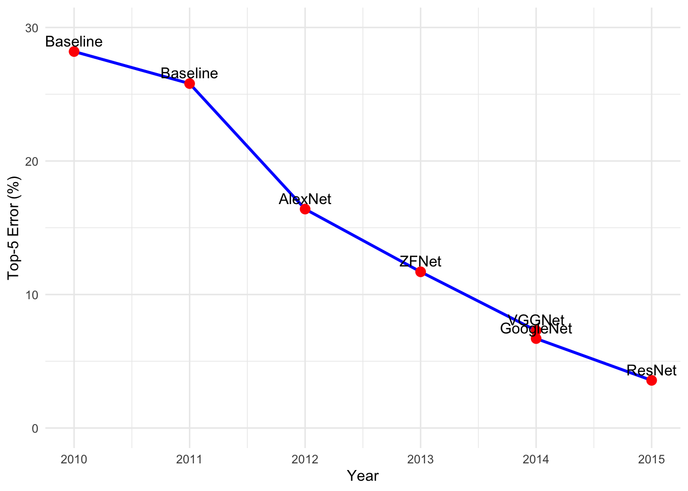](https://mlsysbook.ai/contents/core/benchmarking/benchmarking_files/figure-html/fig-imagenet-challenge-1.png "Figure 1: ImageNet Challenge Progression: Neural networks have reduced error rates from 25.8% in 2010 to 3.57% by 2015, highlighting the impact of architectural advancements on classification accuracy.")
Figure 1: **ImageNet Challenge Progression**: Neural networks have reduced error rates from 25.8% in 2010 to 3.57% by 2015, highlighting the impact of architectural advancements on classification accuracy.
### System Benchmarks
Moving to the second dimension of our framework, we address hardware performance: how efficiently different computational systems execute machine learning workloads. System benchmarks measure the computational foundation that enables algorithmic capabilities, systematically examining how hardware architectures, memory systems, and interconnects affect overall performance. Understanding these hardware limitations and capabilities proves necessary for optimizing the algorithm-system interaction.
AI computations place significant demands on computational resources, far exceeding traditional computing workloads. The underlying hardware infrastructure, encompassing general-purpose CPUs, graphics processing units (GPUs), tensor processing units (TPUs)[7](https://mlsysbook.ai/contents/core/benchmarking/benchmarking.html#fn7)
, and application-specific integrated circuits (ASICs)[8](https://mlsysbook.ai/contents/core/benchmarking/benchmarking.html#fn8)
, determines the speed, efficiency, and scalability of AI solutions. System benchmarks establish standardized methodologies for evaluating hardware performance across AI workloads, measuring metrics including computational throughput, memory bandwidth, power efficiency, and scaling characteristics ([Reddi et al. 2019](https://mlsysbook.ai/contents/core/benchmarking/benchmarking.html#ref-reddi2020mlperf)
; [Mattson et al. 2020](https://mlsysbook.ai/contents/core/benchmarking/benchmarking.html#ref-mattson2020mlperf)
).
7 **Tensor Processing Unit (TPU)**: Google’s custom ASIC designed specifically for neural network workloads, first deployed secretly in 2015 and announced in 2016. The first-generation TPU achieved 15-30x better performance per watt than contemporary GPUs for inference, while TPU v4 pods deliver 1.1 exaFLOPS of BF16 computing power (full pod configuration), demonstrating the capabilities of specialized AI hardware.
8 **Application-Specific Integrated Circuit (ASIC)**: Custom chips designed for specific computational tasks, offering superior performance and energy efficiency compared to general-purpose processors. AI ASICs like Google’s TPUs, Tesla’s FSD chips, and Bitcoin mining ASICs can achieve 100-1000x better efficiency than CPUs for their target applications, but lack the flexibility for other workloads.
Mattson, Peter, Vijay Janapa Reddi, Christine Cheng, Cody Coleman, Greg Diamos, David Kanter, Paulius Micikevicius, et al. 2020. “MLPerf: An Industry Standard Benchmark Suite for Machine Learning Performance.” _IEEE Micro_ 40 (2): 8–16. [https://doi.org/10.1109/mm.2020.2974843](https://doi.org/10.1109/mm.2020.2974843)
.
These system benchmarks perform two critical functions in the AI ecosystem. First, they enable developers and organizations to make informed decisions when selecting hardware platforms for their AI applications by providing comparative performance data across system configurations. Evaluation factors include training speed, inference latency, energy efficiency, and cost-effectiveness. Second, hardware manufacturers rely on these benchmarks to quantify generational improvements and guide the development of specialized AI accelerators, driving advancement in computational capabilities.
**Definition:** Machine Learning System Benchmarks
**_ML System Benchmarks_** are standardized evaluations of _computational infrastructure_ for ML workloads, measuring _performance_, _energy efficiency_, and _scalability_ to enable objective comparison across hardware and software configurations.
However, effective benchmark interpretation requires deep understanding of the performance characteristics inherent to target hardware. Critically, understanding whether specific AI workloads are compute-bound or memory-bound provides essential insight for optimization decisions. Computational intensity, measured as FLOPS[9](https://mlsysbook.ai/contents/core/benchmarking/benchmarking.html#fn9)
per byte of data movement, determines performance limits. Consider an NVIDIA A100 GPU with 312 TFLOPS of tensor performance and 1.6 TB/s memory bandwidth, yielding an arithmetic intensity threshold of 195 FLOPS/byte. The architectural foundations for understanding these hardware characteristics are established in **[Chapter 11: AI Acceleration](https://mlsysbook.ai/contents/core/hw_acceleration/hw_acceleration.html#sec-ai-acceleration)
**, which provides context for interpreting system benchmark results.
9 **FLOPS**: Floating-Point Operations Per Second, a measure of computational performance indicating how many floating-point calculations a processor can execute in one second. Modern AI accelerators achieve high FLOPS ratings: NVIDIA A100 delivers 312 TFLOPS (trillion FLOPS) for tensor operations, while high-end CPUs achieve 1-10 TFLOPS. FLOPS measurements help compare hardware capabilities and determine computational bottlenecks in ML workloads.
Choquette, Jack, Wishwesh Gandhi, Olivier Giroux, Nick Stam, and Ronny Krashinsky. 2021. “NVIDIA A100 Tensor Core GPU: Performance and Innovation.” _IEEE Micro_ 41 (2): 29–35. [https://doi.org/10.1109/mm.2021.3061394](https://doi.org/10.1109/mm.2021.3061394)
.
High-intensity operations like dense matrix multiplication in certain AI model operations (typically >200 FLOPS/byte) achieve near-peak computational throughput on the A100. For example, a ResNet-50 forward pass on large batch sizes (256+) achieves arithmetic intensity of ~300 FLOPS/byte, enabling 85-90% of peak tensor performance (approximately 280 TFLOPS achieved vs 312 TFLOPS theoretical) ([Choquette et al. 2021](https://mlsysbook.ai/contents/core/benchmarking/benchmarking.html#ref-nvidia2020a100)
). Conversely, low-intensity operations like activation functions and certain lightweight operations (<10 FLOPS/byte) become memory bandwidth limited, utilizing only a fraction of the GPU’s computational capacity. A BERT inference with batch size 1 achieves only 8 FLOPS/byte arithmetic intensity, limiting performance to 12.8 TFLOPS (1.6 TB/s × 8 FLOPS/byte), representing just 4% of peak computational capability.
This quantitative analysis, formalized in roofline models[10](https://mlsysbook.ai/contents/core/benchmarking/benchmarking.html#fn10)
, provides a systematic framework that guides both algorithm design and hardware selection by clearly identifying the dominant performance constraints for specific workloads. Understanding these quantitative relationships allows engineers to predict performance bottlenecks accurately and optimize both model architectures and deployment strategies accordingly. For instance, increasing batch size from 1 to 32 for transformer inference can shift operations from memory-bound (8 FLOPS/byte) to compute-bound (150 FLOPS/byte), improving GPU utilization from 4% to 65% ([Pope et al. 2022](https://mlsysbook.ai/contents/core/benchmarking/benchmarking.html#ref-pope2022efficiently)
).
10 **Roofline Model**: A visual performance model developed at UC Berkeley that plots computational intensity (FLOPS/byte) against performance (FLOPS/second) to identify whether algorithms are compute-bound or memory-bound. The “roofline” represents theoretical peak performance limits, with flat sections indicating memory bandwidth constraints and sloped sections showing compute capacity limits. This model helps optimize both algorithms and hardware selection by revealing performance bottlenecks.
Pope, Reiner, Sholto Douglas, Aakanksha Chowdhery, Jacob Devlin, James Bradbury, Anselm Levskaya, Jonathan Heek, Kefan Xiao, Shivani Agrawal, and Jeff Dean. 2022. “Efficiently Scaling Transformer Inference.” _arXiv Preprint arXiv:2211.05102_, November. [http://arxiv.org/abs/2211.05102v1](http://arxiv.org/abs/2211.05102v1)
.
System benchmarks evaluate performance across scales, ranging from single-chip configurations to large distributed systems, and AI workloads including both training and inference tasks. This evaluation approach ensures that benchmarks accurately reflect real-world deployment scenarios and deliver insights that inform both hardware selection decisions and system architecture design. [Figure 2](https://mlsysbook.ai/contents/core/benchmarking/benchmarking.html#fig-imagenet-gpus)
illustrates the correlation between ImageNet classification error rates and GPU adoption from 2010 to 2014. These results highlight how improved hardware capabilities, combined with algorithmic advances, drove progress in computer vision performance.
[](https://mlsysbook.ai/contents/core/benchmarking/511cedd345ba6d417355c7cc4a89ab4230ceebb3.svg "Figure 2: ImageNet Benchmark: Advancements in GPU technology have driven improvements in ImageNet classification accuracy since 2012, showcasing the interplay between hardware and algorithmic progress.")
Figure 2: **ImageNet Benchmark**: Advancements in GPU technology have driven improvements in ImageNet classification accuracy since 2012, showcasing the interplay between hardware and algorithmic progress.
The ImageNet example above demonstrates how hardware advances enable algorithmic breakthroughs, but effective system benchmarking requires understanding the nuanced relationship between workload characteristics and hardware utilization. Modern AI systems rarely achieve theoretical peak performance due to complex interactions between computational patterns, memory hierarchies, and system architectures. This reality gap between theoretical and achieved performance shapes how we design meaningful system benchmarks.
Understanding realistic hardware utilization patterns becomes essential for actionable benchmark design. Different AI workloads interact with hardware architectures in distinctly different ways, creating utilization patterns that vary dramatically based on model architecture, batch size, and precision choices. GPU utilization varies from 85% for well-optimized ResNet-50 training with batch size 64 to only 15% with batch size 1 ([You et al. 2019](https://mlsysbook.ai/contents/core/benchmarking/benchmarking.html#ref-you2019scaling)
) due to insufficient parallelism. Memory bandwidth utilization ranges from 20% for parameter-heavy transformer models to 90% for activation-heavy convolutional networks, directly impacting achievable performance across different precision levels.
You, Yang, Zhao Zhang, Cho-Jui Hsieh, James Demmel, and Kurt Keutzer. 2019. “Scaling SGD Batch Size to 32K for ImageNet Training.” In _Proceedings of Machine Learning and Systems_.
Energy efficiency considerations add another critical dimension to system benchmarking. Performance per watt varies by three orders of magnitude across computing platforms, making energy efficiency a critical benchmark dimension for production deployments. Utilization significantly impacts efficiency: underutilized GPUs consume disproportionate power while delivering minimal performance, creating substantial efficiency penalties that affect operational costs and environmental impact.
Distributed system performance introduces additional complexity that system benchmarks must capture. Traditional roofline models extend to multi-GPU and multi-node scenarios, but distributed training introduces communication bottlenecks that often dominate performance. Inter-node bandwidth limitations, NUMA topology effects, and network congestion create performance variations that single-node benchmarks cannot reveal.
Production distributed systems face challenges that require specialized benchmarking methodologies addressing real-world deployment scenarios. Network partitions during multi-node training affect gradient synchronization and model consistency, requiring fault tolerance evaluation under partial connectivity conditions. Clock synchronization becomes critical for accurate distributed performance measurement across geographically distributed nodes, where timestamp drift can invalidate benchmark results.
Scaling efficiency measurement reveals critical distributed systems bottlenecks in production ML workloads. Linear scaling efficiency degrades significantly beyond 64-128 nodes for most models due to communication overhead: ResNet-50 training achieves 90% scaling efficiency up to 32 nodes but only 60% efficiency at 128 nodes. Gradient aggregation latency increases quadratically with cluster size in traditional parameter server architectures, while all-reduce communication patterns achieve better scaling but require high-bandwidth interconnects.
Consensus mechanisms for benchmark completion across distributed nodes introduce coordination challenges absent from single-node evaluation. Determining benchmark completion requires distributed agreement on convergence criteria, handling node failures during benchmark execution, and ensuring consistent state across all participating nodes. Byzantine fault tolerance becomes necessary for benchmarks spanning multiple administrative domains or cloud providers.
Network topology effects significantly impact distributed training performance in production environments. InfiniBand interconnects achieve 200 Gbps per link with microsecond latency, enabling near-linear scaling for communication-intensive workloads. Ethernet-based clusters with 100 Gbps links experience 10-100x higher latency, limiting scaling efficiency for gradient-heavy models. NUMA topology within nodes creates memory bandwidth contention that affects local gradient computation before network communication.
Dynamic resource allocation in production distributed systems requires benchmarking frameworks that account for resource heterogeneity and temporal variations. Cloud instances with different memory capacities, CPU speeds, and network bandwidth create load imbalance that degrades overall training performance. Spot instance availability fluctuations require fault-tolerant benchmarking that measures recovery time from node failures and resource scaling responsiveness.
These distributed systems considerations highlight the gap between idealized single-node benchmarks and production deployment realities. Effective distributed ML benchmarking must therefore evaluate communication patterns, fault tolerance, resource heterogeneity, and coordination overhead to guide real-world system design decisions.
These hardware utilization insights directly inform benchmark design principles. Effective system benchmarks must evaluate performance across realistic utilization scenarios rather than focusing solely on peak theoretical capabilities. This approach ensures that benchmark results translate to practical deployment guidance, enabling engineers to make informed decisions about hardware selection, system configuration, and optimization strategies.
This transition from computational infrastructure evaluation naturally leads us to the third and equally critical dimension of comprehensive ML system benchmarking: data quality assessment.
### Data Benchmarks
The third dimension of our framework systematically examines data quality, representativeness, and bias in machine learning evaluation. Data benchmarks assess how dataset characteristics affect model performance and reveal critical limitations that may not be apparent from algorithmic or system metrics alone. This dimension is particularly critical because data quality constraints often determine real-world deployment success regardless of algorithmic sophistication or hardware capability.
Data quality, scale, and diversity shape machine learning system performance, directly influencing how effectively algorithms learn and generalize to new situations. To address this dependency, data benchmarks establish standardized datasets and evaluation methodologies that enable consistent comparison of different approaches. These frameworks assess critical aspects of data quality, including domain coverage, potential biases, and resilience to real-world variations in input data ([Gebru et al. 2021](https://mlsysbook.ai/contents/core/benchmarking/benchmarking.html#ref-gebru2021datasheets)
). The data engineering practices necessary for creating reliable benchmarks are detailed in **[Chapter 6: Data Engineering](https://mlsysbook.ai/contents/core/data_engineering/data_engineering.html#sec-data-engineering)
**, while fairness considerations in benchmark design connect to broader responsible AI principles covered in **[Chapter 17: Responsible AI](https://mlsysbook.ai/contents/core/responsible_ai/responsible_ai.html#sec-responsible-ai)
**.
Gebru, Timnit, Jamie Morgenstern, Briana Vecchione, Jennifer Wortman Vaughan, Hanna Wallach, Hal Daumé III, and Kate Crawford. 2021. “Datasheets for Datasets.” _Communications of the ACM_ 64 (12): 86–92. [https://doi.org/10.1145/3458723](https://doi.org/10.1145/3458723)
.
**Definition:** Machine Learning Data Benchmarks
**_ML Data Benchmarks_** are standardized evaluations of _dataset quality_, assessing _coverage_, _bias_, _representativeness_, and _robustness_ to enable objective comparison of data’s impact on model performance.
Data benchmarks serve an essential function in understanding AI system behavior under diverse data conditions. Through systematic evaluation, they help identify common failure modes, expose critical gaps in data coverage, and reveal underlying biases that could significantly impact model behavior in deployment. By providing common frameworks for data evaluation, these benchmarks enable the AI community to systematically improve data quality and address potential issues before deploying systems in production environments. This proactive approach to data quality assessment has become increasingly critical as AI systems take on more complex and consequential tasks across different domains.
### Community-Driven Standardization
Building on our three-dimensional framework, we face a critical challenge created by the proliferation of benchmarks spanning performance, energy efficiency, and domain-specific applications: establishing industry-wide standards. While early computing benchmarks primarily measured simple metrics like processor speed and memory bandwidth, modern benchmarks must evaluate sophisticated aspects of system performance, from complex power consumption profiles to highly specialized application-specific capabilities. This evolution in scope and complexity necessitates comprehensive validation and consensus from the computing community, particularly in rapidly evolving fields like machine learning where performance must be evaluated across multiple interdependent dimensions.
The lasting impact of any benchmark depends critically on its acceptance by the broader research community, where technical excellence alone is insufficient for adoption. Benchmarks developed without broad community input often fail to gain meaningful traction, frequently missing critical metrics that leading research groups consider essential. Successful benchmarks emerge through collaborative development involving academic institutions, industry partners, and domain experts. This inclusive approach ensures benchmarks evaluate capabilities most crucial for advancing the field, while balancing theoretical and practical considerations.
In contrast, benchmarks developed through extensive collaboration among respected institutions carry the authority necessary to drive widespread adoption, while those perceived as advancing particular corporate interests face skepticism and limited acceptance. The remarkable success of ImageNet demonstrates how sustained community engagement through workshops and challenges establishes long-term viability and lasting impact. This community-driven development creates a foundation for formal standardization, where organizations like IEEE and ISO transform these benchmarks into official standards.
The standardization process provides crucial infrastructure for benchmark formalization and adoption. [IEEE working groups](https://standards.ieee.org/develop/wg/)
transform community-developed benchmarking methodologies into formal industry standards, establishing precise specifications for measurement and reporting. The [IEEE 2416-2019](https://standards.ieee.org/ieee/2416/7065/)
standard for system power modeling exemplifies this process, codifying best practices developed through community consensus. Similarly, [ISO/IEC technical committees](https://www.iso.org/committee/45020.html)
develop international standards for benchmark validation and certification, ensuring consistent evaluation across global research and industry communities. These organizations bridge the gap between community-driven innovation and formal standardization, providing frameworks that enable reliable comparison of results across different institutions and geographic regions.
Successful community benchmarks establish clear governance structures for managing their evolution. Through rigorous version control systems and detailed change documentation, benchmarks maintain backward compatibility while incorporating new advances. This governance includes formal processes for proposing, reviewing, and implementing changes, ensuring that benchmarks remain relevant while maintaining stability. Modern benchmarks increasingly emphasize reproducibility requirements, incorporating automated verification systems and standardized evaluation environments.
Open access accelerates benchmark adoption and ensures consistent implementation. Projects that provide open-source reference implementations, comprehensive documentation, validation suites, and containerized evaluation environments reduce barriers to entry. This standardization enables research groups to evaluate solutions using uniform methods and metrics. Without such coordinated implementation frameworks, organizations might interpret benchmarks inconsistently, compromising result reproducibility and meaningful comparison across studies.
The most successful benchmarks strike a careful balance between academic rigor and industry practicality. Academic involvement ensures theoretical soundness and comprehensive evaluation methodology, while industry participation grounds benchmarks in practical constraints and real-world applications. This balance proves particularly crucial in machine learning benchmarks, where theoretical advances must translate to practical improvements in deployed systems ([Patterson et al. 2021](https://mlsysbook.ai/contents/core/benchmarking/benchmarking.html#ref-patterson2021carbon)
). These evaluation methodology principles guide both training and inference benchmark design throughout this chapter.
Community consensus establishes enduring benchmark relevance, while fragmentation impedes scientific progress. Through collaborative development and transparent operation, benchmarks evolve into authoritative standards for measuring advancement. The most successful benchmarks in energy efficiency and domain-specific applications share this foundation of community development and governance, demonstrating how collective expertise and shared purpose create lasting impact in rapidly advancing fields.
**Self-Check: Question 1.3**
1. What is a key difference between traditional benchmarks and AI benchmarks?
1. AI benchmarks focus solely on computational speed.
2. Traditional benchmarks include data quality as a primary factor.
3. AI benchmarks incorporate variability and accuracy as evaluation dimensions.
4. Traditional benchmarks are more complex than AI benchmarks.
2. Explain why energy efficiency is considered a cross-cutting concern in the three-dimensional evaluation framework for ML benchmarks.
3. True or False: The inherent variability in ML systems makes it unnecessary to run multiple experimental trials when benchmarking.
4. Order the following steps for effective ML benchmarking: (1) Evaluate algorithmic performance, (2) Measure system performance, (3) Assess data quality.
[See Answers →](https://mlsysbook.ai/contents/core/benchmarking/benchmarking.html#quiz-answer-sec-benchmarking-ai-machine-learning-benchmarks-6b88)
Benchmarking Granularity
------------------------
The three-dimensional framework and measurement foundations established above provide the conceptual structure for benchmarking. However, implementing these principles requires choosing the appropriate level of detail for evaluation, from individual tensor operations to complete ML applications. Just as the optimization techniques from **[Chapter 10: Model Optimizations](https://mlsysbook.ai/contents/core/optimizations/optimizations.html#sec-model-optimizations)
** operate at different granularities, benchmarks must adapt their evaluation scope to match specific optimization goals. This hierarchical perspective allows practitioners to isolate performance bottlenecks at the micro level or assess system-wide behavior at the macro level.
System level benchmarking provides a structured and systematic approach to assessing a ML system’s performance across various dimensions. Given the complexity of ML systems, we can dissect their performance through different levels of granularity and obtain a comprehensive view of the system’s efficiency, identify potential bottlenecks, and pinpoint areas for improvement. To this end, various types of benchmarks have evolved over the years and continue to persist.
[Figure 3](https://mlsysbook.ai/contents/core/benchmarking/benchmarking.html#fig-granularity)
shows the different layers of granularity of an ML system. At the application level, end-to-end benchmarks assess the overall system performance, considering factors like data preprocessing, model training, and inference. While at the model layer, benchmarks focus on assessing the efficiency and accuracy of specific models. This includes evaluating how well models generalize to new data and their computational efficiency during training and inference. Benchmarking can extend to hardware and software infrastructure, examining the performance of individual components like GPUs or TPUs.
[](https://mlsysbook.ai/contents/core/benchmarking/1c82424cb3c277044c442f5efd75773e1f848e30.svg "Figure 3: Benchmarking Granularity: ML system performance assessment occurs at multiple levels, from end-to-end application metrics to individual model and hardware component efficiency, enabling targeted optimization and bottleneck identification. This hierarchical approach allows practitioners to systematically analyze system performance and prioritize improvements based on specific component limitations.")
Figure 3: **Benchmarking Granularity**: ML system performance assessment occurs at multiple levels, from end-to-end application metrics to individual model and hardware component efficiency, enabling targeted optimization and bottleneck identification. This hierarchical approach allows practitioners to systematically analyze system performance and prioritize improvements based on specific component limitations.
### Micro Benchmarks
Micro-benchmarks are specialized evaluation tools that assess distinct components or specific operations within a broader machine learning process. These benchmarks isolate individual tasks to provide detailed insights into the computational demands of particular system elements, from neural network layers to optimization techniques to activation functions. For example, micro-benchmarks might measure the time required to execute a convolutional layer in a deep learning model or evaluate the speed of data preprocessing operations that prepare training data.
A key area of micro-benchmarking focuses on tensor operations[11](https://mlsysbook.ai/contents/core/benchmarking/benchmarking.html#fn11)
, which are the computational core of deep learning. Libraries like [cuDNN](https://developer.nvidia.com/cudnn)
[12](https://mlsysbook.ai/contents/core/benchmarking/benchmarking.html#fn12)
by NVIDIA provide benchmarks for measuring fundamental computations such as convolutions and matrix multiplications across different hardware configurations. These measurements help developers understand how their hardware handles the core mathematical operations that dominate ML workloads.
11 **Tensor Operations**: Multi-dimensional array computations that form the backbone of neural networks, including matrix multiplication (GEMM), convolution, and element-wise operations. Modern AI accelerators optimize these primitives: NVIDIA’s Tensor Cores can achieve 312 TFLOPS for mixed-precision matrix multiplications (BF16), compared to 15-20 TFLOPS for traditional FP32 computations, representing approximately 15-20x speedup.
12 **cuDNN**: CUDA Deep Neural Network library, NVIDIA’s GPU-accelerated library of primitives for deep neural networks. Released in 2014, cuDNN provides highly optimized implementations for convolutions, pooling, normalization, and activation layers, delivering up to 10x performance improvements over naive implementations and becoming the de facto standard for GPU-accelerated deep learning.
13 **Sigmoid Function**: A mathematical activation function S(x) = 1/(1+e^(-x)) that maps any real number to a value between 0 and 1, historically important in early neural networks. Despite being computationally expensive due to exponential operations and suffering from vanishing gradient problems, sigmoid functions remain relevant for binary classification output layers and gates in LSTM cells.
14 **Tanh Function**: Hyperbolic tangent activation function tanh(x) = (e^x - e(-x))/(ex + e^(-x)) that maps inputs to values between -1 and 1, providing zero-centered outputs unlike sigmoid. While computationally intensive and still subject to vanishing gradients, tanh often performs better than sigmoid in hidden layers due to stronger gradients and symmetric output range.
15 **LSTM (Long Short-Term Memory)**: A type of recurrent neural network architecture introduced by Hochreiter and Schmidhuber in 1997, designed to solve the vanishing gradient problem in traditional RNNs. LSTMs use gates (forget, input, output) to control information flow, enabling them to learn dependencies over hundreds of time steps, making them crucial for sequence modeling before the Transformer era.
Micro-benchmarks also examine activation functions and neural network layers in isolation. This includes measuring the performance of various activation functions like ReLU, Sigmoid[13](https://mlsysbook.ai/contents/core/benchmarking/benchmarking.html#fn13)
, and Tanh[14](https://mlsysbook.ai/contents/core/benchmarking/benchmarking.html#fn14)
under controlled conditions, as well as evaluating the computational efficiency of distinct neural network components such as LSTM[15](https://mlsysbook.ai/contents/core/benchmarking/benchmarking.html#fn15)
cells or Transformer blocks when processing standardized inputs.
[DeepBench](https://github.com/baidu-research/DeepBench)
, developed by Baidu, was one of the first to demonstrate the value of comprehensive micro-benchmarking. It evaluates these fundamental operations across different hardware platforms, providing detailed performance data that helps developers optimize their deep learning implementations. By isolating and measuring individual operations, DeepBench enables precise comparison of hardware platforms and identification of potential performance bottlenecks.
### Macro Benchmarks
While micro-benchmarks examine individual operations like tensor computations and layer performance, macro benchmarks evaluate complete machine learning models. This shift from component-level to model-level assessment provides insights into how architectural choices and component interactions affect overall model behavior. For instance, while micro-benchmarks might show optimal performance for individual convolutional layers, macro-benchmarks reveal how these layers work together within a complete convolutional neural network.
Macro-benchmarks measure multiple performance dimensions that emerge only at the model level. These include prediction accuracy, which shows how well the model generalizes to new data; memory consumption patterns across different batch sizes and sequence lengths; throughput under varying computational loads; and latency across different hardware configurations. Understanding these metrics helps developers make informed decisions about model architecture, optimization strategies, and deployment configurations.
The assessment of complete models occurs under standardized conditions using established datasets and tasks. For example, computer vision models might be evaluated on [ImageNet](https://www.image-net.org/)
, measuring both computational efficiency and prediction accuracy. Natural language processing models might be assessed on translation tasks, examining how they balance quality and speed across different language pairs.
Several industry-standard benchmarks enable consistent model evaluation across platforms. [MLPerf Inference](https://github.com/mlcommons/inference)
provides comprehensive testing suites adapted for different computational environments ([Reddi et al. 2019](https://mlsysbook.ai/contents/core/benchmarking/benchmarking.html#ref-reddi2020mlperf)
). [MLPerf Mobile](https://github.com/mlcommons/mobile_app_open)
focuses on mobile device constraints ([Janapa Reddi et al. 2022](https://mlsysbook.ai/contents/core/benchmarking/benchmarking.html#ref-janapa2022mlperf)
), while [MLPerf Tiny](https://github.com/mlcommons/tiny)
addresses microcontroller deployments ([Banbury et al. 2021](https://mlsysbook.ai/contents/core/benchmarking/benchmarking.html#ref-banbury2021mlperf)
). For embedded systems, [EEMBC’s MLMark](https://github.com/eembc/mlmark)
emphasizes both performance and power efficiency. The [AI-Benchmark](https://ai-benchmark.com/)
suite specializes in mobile platforms, evaluating models across diverse tasks from image recognition to face parsing.
Janapa Reddi, Vijay et al. 2022. “MLPerf Mobile V2. 0: An Industry-Standard Benchmark Suite for Mobile Machine Learning.” In _Proceedings of Machine Learning and Systems_, 4:806–23.
Banbury, Colby, Vijay Janapa Reddi, Peter Torelli, Jeremy Holleman, Nat Jeffries, Csaba Kiraly, Pietro Montino, et al. 2021. “MLPerf Tiny Benchmark.” _arXiv Preprint arXiv:2106.07597_, June. [http://arxiv.org/abs/2106.07597v4](http://arxiv.org/abs/2106.07597v4)
.
### End-to-End Benchmarks
End-to-end benchmarks provide an all-inclusive evaluation that extends beyond the boundaries of the ML model itself. Rather than focusing solely on a machine learning model’s computational efficiency or accuracy, these benchmarks encompass the entire pipeline of an AI system. This includes initial ETL (Extract-Transform-Load) or ELT (Extract-Load-Transform) data processing, the core model’s performance, post-processing of results, and critical infrastructure components like storage and network systems.
Data processing is the foundation of all AI systems, transforming raw data into a format suitable for model training or inference. In ETL pipelines, data undergoes extraction from source systems, transformation through cleaning and feature engineering, and loading into model-ready formats. These preprocessing steps’ efficiency, scalability, and accuracy significantly impact overall system performance. End-to-end benchmarks must assess standardized datasets through these pipelines to ensure data preparation doesn’t become a bottleneck.
The post-processing phase plays an equally important role. This involves interpreting the model’s raw outputs, converting scores into meaningful categories, filtering results based on predefined tasks, or integrating with other systems. For instance, a computer vision system might need to post-process detection boundaries, apply confidence thresholds, and format results for downstream applications. In real-world deployments, this phase proves crucial for delivering actionable insights.
Beyond core AI operations, infrastructure components heavily influence overall performance and user experience. Storage solutions, whether cloud-based, on-premises, or hybrid, can significantly impact data retrieval and storage times, especially with vast AI datasets. Network interactions, vital for distributed systems, can become performance bottlenecks if not optimized. End-to-end benchmarks must evaluate these components under specified environmental conditions to ensure reproducible measurements of the entire system.
To date, there are no public, end-to-end benchmarks that fully account for data storage, network, and compute performance. While MLPerf Training and Inference approach end-to-end evaluation, they primarily focus on model performance rather than real-world deployment scenarios. Nonetheless, they provide valuable baseline metrics for assessing AI system capabilities.
Given the inherent specificity of end-to-end benchmarking, organizations typically perform these evaluations internally by instrumenting production deployments. This allows engineers to develop result interpretation guidelines based on realistic workloads, but given the sensitivity and specificity of the information, these benchmarks rarely appear in public settings.
### Granularity Trade-offs and Selection Criteria
As shown in [Table 1](https://mlsysbook.ai/contents/core/benchmarking/benchmarking.html#tbl-benchmark-comparison)
, different challenges emerge at different stages of an AI system’s lifecycle. Each benchmarking approach provides unique insights: micro-benchmarks help engineers optimize specific components like GPU kernel implementations or data loading operations, macro-benchmarks guide model architecture decisions and algorithm selection, while end-to-end benchmarks reveal system-level bottlenecks in production environments.
Table 1: **Benchmarking Granularity Levels**: Different benchmark scopes (micro, macro, and end-to-end) target distinct stages of ML system development and reveal unique performance bottlenecks. Micro-benchmarks isolate individual operations for low-level optimization, macro-benchmarks evaluate complete models to guide architectural choices, and end-to-end benchmarks assess full system performance in production environments.
| | | | |
| --- | --- | --- | --- |
| **Focus** | Individual operations | Complete models | Full system pipeline |
| **Scope** | Tensor ops, layers, activations | Model architecture, training, inference | ETL, model, infrastructure |
| **Example** | Conv layer performance on cuDNN | ResNet-50 on ImageNet | Production recommendation system |
| **Advantages** | Precise bottleneck identification, Component optimization | Model architecture comparison, Standardized evaluation | Realistic performance assessment, System-wide insights |
| **Challenges** | May miss interaction effects | Limited infrastructure insights | Complex to standardize, Often proprietary |
| **Typical Use** | Hardware selection, Operation optimization | Model selection, Research comparison | Production system evaluation |
[Figure 4](https://mlsysbook.ai/contents/core/benchmarking/benchmarking.html#fig-benchmark-tradeoffs)
visualizes the core trade-off between diagnostic power and real-world representativeness across benchmark granularity levels. This relationship illustrates why comprehensive ML system evaluation requires multiple benchmark types: micro-benchmarks provide precise optimization guidance for isolated components, while end-to-end benchmarks capture the complex interactions that emerge in production systems. The optimal benchmarking strategy combines insights from all three levels to balance detailed component analysis with realistic system-wide assessment.
[](https://mlsysbook.ai/contents/core/benchmarking/14c89654f94afa5679667542ce6b75fe1027c825.svg "Figure 4: Benchmark Granularity Trade-offs: The core trade-off in benchmarking granularity between isolation/diagnostic power and real-world representativeness. Micro-benchmarks provide high diagnostic precision but limited real-world relevance, while end-to-end benchmarks capture realistic system behavior but offer less precise component-level insights. Effective ML system evaluation requires strategic combination of all three levels.")
Figure 4: **Benchmark Granularity Trade-offs**: The core trade-off in benchmarking granularity between isolation/diagnostic power and real-world representativeness. Micro-benchmarks provide high diagnostic precision but limited real-world relevance, while end-to-end benchmarks capture realistic system behavior but offer less precise component-level insights. Effective ML system evaluation requires strategic combination of all three levels.
Component interaction often produces unexpected behaviors. For example, while micro-benchmarks might show excellent performance for individual convolutional layers, and macro-benchmarks might demonstrate strong accuracy for the complete model, end-to-end evaluation could reveal that data preprocessing creates unexpected bottlenecks during high-traffic periods. These system-level insights often remain hidden when components undergo isolated testing.
With benchmarking granularity established, understanding which level of evaluation serves specific optimization goals, we now examine the concrete components that constitute benchmark implementations at any granularity level.
**Self-Check: Question 1.4**
1. Which of the following best describes the purpose of micro-benchmarks in ML systems?
1. To evaluate the entire ML pipeline for production readiness.
2. To assess individual operations like tensor computations for optimization.
3. To compare different ML models on standard datasets.
4. To evaluate the performance of storage and network systems.
2. Discuss the trade-offs between micro-benchmarks and end-to-end benchmarks in ML systems.
3. Order the following benchmarking levels from most isolated to most comprehensive: (1) Macro-benchmarks, (2) Micro-benchmarks, (3) End-to-end benchmarks.
4. What is a primary challenge of using end-to-end benchmarks in ML systems?
1. They provide too much detail on individual operations.
2. They often miss system-level bottlenecks.
3. They focus only on model accuracy, ignoring infrastructure.
4. They are complex to standardize and often proprietary.
[See Answers →](https://mlsysbook.ai/contents/core/benchmarking/benchmarking.html#quiz-answer-sec-benchmarking-ai-benchmarking-granularity-771c)
Benchmark Components
--------------------
Using our established framework, we now examine the practical components that constitute any benchmark implementation. These components provide the concrete structure for measuring performance across all three dimensions simultaneously. Whether evaluating model accuracy (algorithmic dimension), measuring inference latency (system dimension), or assessing dataset quality (data dimension), benchmarks share common structural elements that ensure systematic and reproducible evaluation.
The granularity level established in the previous section directly shapes how these components are instantiated. Micro-benchmarks measuring tensor operations require synthetic inputs that isolate specific computational patterns, enabling precise performance characterization of individual kernels as discussed in **[Chapter 11: AI Acceleration](https://mlsysbook.ai/contents/core/hw_acceleration/hw_acceleration.html#sec-ai-acceleration)
**. Macro-benchmarks evaluating complete models demand representative datasets like ImageNet that capture realistic task complexity while enabling standardized comparison across architectures. End-to-end benchmarks assessing production systems must incorporate real-world data characteristics including distribution shift, noise, and edge cases absent from curated evaluation sets. Similarly, evaluation metrics shift focus across granularity levels: micro-benchmarks emphasize FLOPS and memory bandwidth utilization, macro-benchmarks balance accuracy and inference speed, while end-to-end benchmarks prioritize system reliability and operational efficiency under load. Understanding this systematic variation ensures that component choices align with evaluation objectives rather than applying uniform approaches across different benchmarking scales.
Having established how benchmark granularity shapes evaluation scope (from micro-benchmarks isolating tensor operations to end-to-end assessments of complete systems), we now examine how these conceptual levels translate into concrete benchmark implementations. The components discussed abstractly above must be instantiated through specific choices about tasks, datasets, models, and metrics. This implementation process follows a systematic workflow that ensures reproducible and meaningful evaluation regardless of the chosen granularity level.
An AI benchmark provides this structured framework for systematically evaluating artificial intelligence systems. While individual benchmarks vary significantly in their specific focus and granularity, they share common implementation components that enable consistent evaluation and comparison across different approaches.
[Figure 5](https://mlsysbook.ai/contents/core/benchmarking/benchmarking.html#fig-benchmark-components)
illustrates this structured workflow, showcasing how the essential components (task definition, dataset selection, model selection, and evaluation metrics) interconnect to form a complete evaluation pipeline. Each component builds upon the previous one, creating a systematic progression from problem specification through deployment assessment.
[](https://mlsysbook.ai/contents/core/benchmarking/e5884436bf0c353082158de1ad5aacf03a570eef.svg "Figure 5: Benchmark Workflow: AI benchmarks standardize evaluation through a structured pipeline, enabling reproducible performance comparisons across different models and systems. This workflow systematically assesses AI capabilities by defining tasks, selecting datasets, training models, and rigorously evaluating results.")
Figure 5: **Benchmark Workflow**: AI benchmarks standardize evaluation through a structured pipeline, enabling reproducible performance comparisons across different models and systems. This workflow systematically assesses AI capabilities by defining tasks, selecting datasets, training models, and rigorously evaluating results.
Effective benchmark design must account for the optimization techniques established in preceding chapters. Quantization and pruning affect model accuracy-efficiency trade-offs, requiring benchmarks that measure both speedup and accuracy preservation simultaneously. Hardware acceleration techniques influence arithmetic intensity and memory bandwidth utilization, necessitating roofline model analysis to interpret results correctly. Understanding these optimization foundations enables benchmark selection that validates claimed improvements rather than measuring artificial scenarios.
### Problem Definition
As illustrated in [Figure 5](https://mlsysbook.ai/contents/core/benchmarking/benchmarking.html#fig-benchmark-components)
, a benchmark implementation begins with a formal specification of the machine learning task and its evaluation criteria. In machine learning, tasks represent well-defined problems that AI systems must solve. Consider an anomaly detection system that processes audio signals to identify deviations from normal operation patterns, as shown in [Figure 5](https://mlsysbook.ai/contents/core/benchmarking/benchmarking.html#fig-benchmark-components)
. This industrial monitoring application exemplifies how formal task specifications translate into practical implementations.
The formal definition of any benchmark task encompasses both the computational problem and its evaluation framework. While the specific tasks vary significantly by domain, well-established categories have emerged across major fields of AI research. Natural language processing tasks, for example, include machine translation, question answering ([Hirschberg and Manning 2015](https://mlsysbook.ai/contents/core/benchmarking/benchmarking.html#ref-hirschberg2015advances)
), and text classification. Computer vision similarly employs standardized tasks such as object detection, image segmentation, and facial recognition ([Everingham et al. 2009](https://mlsysbook.ai/contents/core/benchmarking/benchmarking.html#ref-everingham2010pascal)
).
Hirschberg, Julia, and Christopher D. Manning. 2015. “Advances in Natural Language Processing.” _Science_ 349 (6245): 261–66. [https://doi.org/10.1126/science.aaa8685](https://doi.org/10.1126/science.aaa8685)
.
Everingham, Mark, Luc Van Gool, Christopher K. I. Williams, John Winn, and Andrew Zisserman. 2009. “The Pascal Visual Object Classes (VOC) Challenge.” _International Journal of Computer Vision_ 88 (2): 303–38. [https://doi.org/10.1007/s11263-009-0275-4](https://doi.org/10.1007/s11263-009-0275-4)
.
Every benchmark task specification must define three essential elements. The input specification determines what data the system processes. In [Figure 5](https://mlsysbook.ai/contents/core/benchmarking/benchmarking.html#fig-benchmark-components)
, this consists of audio waveform data. The output specification describes the required system response, such as the binary classification of normal versus anomalous patterns. The performance specification establishes quantitative requirements for accuracy, processing speed, and resource utilization.
Task design directly impacts the benchmark’s ability to evaluate AI systems effectively. The audio anomaly detection example clearly illustrates this relationship through its specific requirements: processing continuous signal data, adapting to varying noise conditions, and operating within strict time constraints. These practical constraints create a detailed framework for assessing model performance, ensuring evaluations reflect real-world operational demands.
The implementation of a benchmark proceeds systematically from this foundational task definition. Each subsequent phase, from dataset selection through deployment, builds directly upon these initial specifications, ensuring that evaluations maintain consistency while addressing the defined requirements across different approaches and implementations.
### Standardized Datasets
Building directly upon the problem definition established in the previous phase, standardized datasets provide the essential foundation for training and evaluating models. These carefully curated collections ensure all models undergo testing under identical conditions, enabling direct comparisons across different approaches and architectures. [Figure 5](https://mlsysbook.ai/contents/core/benchmarking/benchmarking.html#fig-benchmark-components)
demonstrates this through an audio anomaly detection example, where waveform data serves as the standardized input for evaluating detection performance.
In computer vision, datasets such as [ImageNet](http://www.image-net.org/)
([Deng et al. 2009](https://mlsysbook.ai/contents/core/benchmarking/benchmarking.html#ref-deng2009imagenet)
), [COCO](https://cocodataset.org/)
([Lin et al. 2014](https://mlsysbook.ai/contents/core/benchmarking/benchmarking.html#ref-lin2014microsoft)
), and [CIFAR-10](https://www.cs.toronto.edu/~kriz/cifar.html)
[16](https://mlsysbook.ai/contents/core/benchmarking/benchmarking.html#fn16)
([Krizhevsky, Hinton, et al. 2009](https://mlsysbook.ai/contents/core/benchmarking/benchmarking.html#ref-krizhevsky2009learning)
) serve as reference standards. For natural language processing, collections such as [SQuAD](https://rajpurkar.github.io/SQuAD-explorer/)
[17](https://mlsysbook.ai/contents/core/benchmarking/benchmarking.html#fn17)
([Rajpurkar et al. 2016](https://mlsysbook.ai/contents/core/benchmarking/benchmarking.html#ref-rajpurkar2016squad)
), [GLUE](https://gluebenchmark.com/)
[18](https://mlsysbook.ai/contents/core/benchmarking/benchmarking.html#fn18)
([Wang et al. 2018](https://mlsysbook.ai/contents/core/benchmarking/benchmarking.html#ref-wang2018glue)
), and [WikiText](https://www.salesforce.com/blog/the-wikitext-long-term-dependency-language-modeling-dataset/)
([Merity et al. 2016](https://mlsysbook.ai/contents/core/benchmarking/benchmarking.html#ref-merity2016pointer)
) fulfill similar functions. These datasets encompass a range of complexities and edge cases to thoroughly evaluate machine learning systems.
16 **CIFAR-10**: A dataset of 60,000 32×32 color images across 10 classes (airplane, automobile, bird, cat, deer, dog, frog, horse, ship, truck), collected by Alex Krizhevsky and Geoffrey Hinton at the University of Toronto in 2009. Despite its small image size, CIFAR-10 became fundamental for comparing deep learning architectures, with top-1 error rates improving from 18.5% with traditional methods to 2.6% with modern deep networks.
Krizhevsky, Alex, Geoffrey Hinton, et al. 2009. “Learning Multiple Layers of Features from Tiny Images.”
17 **SQuAD**: Stanford Question Answering Dataset, introduced in 2016, containing 100,000+ question-answer pairs based on Wikipedia articles. SQuAD became the gold standard for evaluating reading comprehension, with human performance at 87.4% F1 score and leading AI systems achieving over 90% by 2018, marking the first time machines exceeded human performance on this benchmark.
Rajpurkar, Pranav, Jian Zhang, Konstantin Lopyrev, and Percy Liang. 2016. “SQuAD: 100,000+ Questions for Machine Comprehension of Text.” _arXiv Preprint arXiv:1606.05250_, June, 2383–92. [https://doi.org/10.18653/v1/d16-1264](https://doi.org/10.18653/v1/d16-1264)
.
18 **GLUE**: General Language Understanding Evaluation, a collection of nine English sentence understanding tasks including sentiment analysis, textual entailment, and similarity. Introduced in 2018, GLUE provided standardized evaluation with a human baseline of 87.1% and became obsolete when BERT achieved 80.5% in 2019, leading to the more challenging SuperGLUE benchmark.
Merity, Stephen, Caiming Xiong, James Bradbury, and Richard Socher. 2016. “Pointer Sentinel Mixture Models.” _arXiv Preprint arXiv:1609.07843_, September. [http://arxiv.org/abs/1609.07843v1](http://arxiv.org/abs/1609.07843v1)
.
The strategic selection of datasets, shown early in the workflow of [Figure 5](https://mlsysbook.ai/contents/core/benchmarking/benchmarking.html#fig-benchmark-components)
, shapes all subsequent implementation steps and ultimately determines the benchmark’s effectiveness. In the audio anomaly detection example, the dataset must include representative waveform samples of normal operation alongside comprehensive examples of various anomalous conditions. Notable examples include datasets like ToyADMOS for industrial manufacturing anomalies and Google Speech Commands for general sound recognition. Regardless of the specific dataset chosen, the data volume must suffice for both model training and validation, while incorporating real-world signal characteristics and noise patterns that reflect deployment conditions.
The selection of benchmark datasets directly shapes experimental outcomes and model evaluation. Effective datasets must balance two key requirements: accurately representing real-world challenges while maintaining sufficient complexity to differentiate model performance meaningfully. While research often utilizes simplified datasets like ToyADMOS[19](https://mlsysbook.ai/contents/core/benchmarking/benchmarking.html#fn19)
([Koizumi et al. 2019](https://mlsysbook.ai/contents/core/benchmarking/benchmarking.html#ref-koizumi2019toyadmos)
), these controlled environments, though valuable for methodological development, may not fully capture real-world deployment complexities.
19 **ToyADMOS**: A dataset for anomaly detection in machine operating sounds, developed by NTT Communications in 2019 containing audio recordings from toy car and toy conveyor belt operations. The dataset includes 1,000+ normal samples and 300+ anomalous samples per machine type, designed to standardize acoustic anomaly detection research with reproducible experimental conditions.
Koizumi, Yuma, Shoichiro Saito, Hisashi Uematsu, Noboru Harada, and Keisuke Imoto. 2019. “ToyADMOS: A Dataset of Miniature-Machine Operating Sounds for Anomalous Sound Detection.” In _2019 IEEE Workshop on Applications of Signal Processing to Audio and Acoustics (WASPAA)_, 313–17. IEEE; IEEE. [https://doi.org/10.1109/waspaa.2019.8937164](https://doi.org/10.1109/waspaa.2019.8937164)
.
### Model Selection
Following dataset specification, the benchmark process advances systematically to model architecture selection and implementation. This critical phase establishes performance baselines and determines the optimal modeling approach for the specific task at hand. The selection process directly builds upon the architectural foundations established in **[Chapter 4: DNN Architectures](https://mlsysbook.ai/contents/core/dnn_architectures/dnn_architectures.html#sec-dnn-architectures)
** and must account for the framework-specific considerations discussed in **[Chapter 7: AI Frameworks](https://mlsysbook.ai/contents/core/frameworks/frameworks.html#sec-ai-frameworks)
**. [Figure 5](https://mlsysbook.ai/contents/core/benchmarking/benchmarking.html#fig-benchmark-components)
illustrates this progression through the model selection stage and subsequent training code development.
Baseline models serve as the reference points for evaluating novel approaches. These span from basic implementations, including linear regression for continuous predictions and logistic regression for classification tasks, to advanced architectures with proven success in comparable domains. The choice of baseline depends critically on the deployment framework—a PyTorch implementation may exhibit different performance characteristics than its TensorFlow equivalent due to framework-specific optimizations and operator implementations. In natural language processing applications, advanced language models like BERT[20](https://mlsysbook.ai/contents/core/benchmarking/benchmarking.html#fn20)
have emerged as standard benchmarks for comparative analysis. The architectural details of transformers and their performance characteristics are thoroughly covered in **[Chapter 4: DNN Architectures](https://mlsysbook.ai/contents/core/dnn_architectures/dnn_architectures.html#sec-dnn-architectures)
**.
20 **BERT**: Bidirectional Encoder Representations from Transformers, introduced by Google in 2018, revolutionized natural language processing by pre-training on vast text corpora using masked language modeling. BERT-Large contains 340 million parameters and achieved state-of-the-art results on 11 NLP tasks, establishing the foundation for modern language models like GPT and ChatGPT.
Selecting the right baseline model requires careful evaluation of architectures against benchmark requirements. This selection process directly informs the development of training code, which is the cornerstone of benchmark reproducibility. The training implementation must thoroughly document all aspects of the model pipeline, from data preprocessing through training procedures, enabling precise replication of model behavior across research teams.
With model architecture selected, model development follows two primary optimization paths: training and inference. During training optimization, efforts concentrate on achieving target accuracy metrics while operating within computational constraints. The training implementation must demonstrate consistent achievement of performance thresholds under specified conditions.
In parallel, the inference optimization path addresses deployment considerations, particularly the critical transition from development to production environments. A key example involves precision reduction through numerical optimization techniques, progressing from high-precision to lower-precision representations to enhance deployment efficiency. This process demands careful calibration to maintain model accuracy while reducing resource requirements. The benchmark must detail both the quantization methodology and verification procedures that confirm preserved performance.
The intersection of these two optimization paths with real-world constraints shapes overall deployment strategy. Comprehensive benchmarks must therefore specify requirements for both training and inference scenarios, ensuring models maintain consistent performance from development through deployment. This crucial connection between development and production metrics naturally leads to the establishment of evaluation criteria.
The optimization process must balance four key objectives: model accuracy, computational speed, memory utilization, and energy efficiency. Following our three-dimensional benchmarking framework, this complex optimization landscape necessitates robust evaluation metrics that can effectively quantify performance across algorithmic, system, and data dimensions. As models transition from development to deployment, these metrics serve as critical tools for guiding optimization decisions and validating performance enhancements.
### Evaluation Metrics
Building upon the optimization framework established through model selection, evaluation metrics provide the quantitative measures needed to assess machine learning model performance. These metrics establish objective standards for comparing different approaches, allowing researchers and practitioners to gauge solution effectiveness. The selection of appropriate metrics represents a critical aspect of benchmark design, as they must align with task objectives while providing meaningful insights into model behavior across both training and deployment scenarios. Importantly, metric computation can vary between frameworks—the training methodologies from **[Chapter 8: AI Training](https://mlsysbook.ai/contents/core/training/training.html#sec-ai-training)
** demonstrate how different frameworks handle loss computation and gradient accumulation differently, affecting reported metrics.
Task-specific metrics quantify a model’s performance on its intended function. For example, classification tasks employ metrics including accuracy (overall correct predictions), precision (positive prediction accuracy), recall (positive case detection rate), and F1 score (precision-recall harmonic mean) ([Sokolova and Lapalme 2009](https://mlsysbook.ai/contents/core/benchmarking/benchmarking.html#ref-sokolova2009systematic)
). Regression problems utilize error measurements like Mean Squared Error (MSE) and Mean Absolute Error (MAE) to assess prediction accuracy. Domain-specific applications often require specialized metrics - for example, machine translation uses the BLEU score[21](https://mlsysbook.ai/contents/core/benchmarking/benchmarking.html#fn21)
to evaluate the semantic and syntactic similarity between machine-generated and human reference translations ([Papineni et al. 2001](https://mlsysbook.ai/contents/core/benchmarking/benchmarking.html#ref-papineni2002bleu)
).
Sokolova, Marina, and Guy Lapalme. 2009. “A Systematic Analysis of Performance Measures for Classification Tasks.” _Information Processing &Amp; Management_ 45 (4): 427–37. [https://doi.org/10.1016/j.ipm.2009.03.002](https://doi.org/10.1016/j.ipm.2009.03.002)
.
21 **BLEU Score**: Bilingual Evaluation Understudy, introduced by IBM in 2002, measures machine translation quality by comparing n-gram overlap between machine and human reference translations. BLEU scores range from 0-100, with scores above 30 considered useful, above 50 good, and above 60 high quality. Google Translate achieved BLEU scores of 40+ on major language pairs by 2016.
Papineni, Kishore, Salim Roukos, Todd Ward, and Wei-Jing Zhu. 2001. “BLEU: A Method for Automatic Evaluation of Machine Translation.” In _Proceedings of the 40th Annual Meeting on Association for Computational Linguistics - ACL ’02_, 311. Association for Computational Linguistics. [https://doi.org/10.3115/1073083.1073135](https://doi.org/10.3115/1073083.1073135)
.
However, as models transition from research to production deployment, implementation metrics become equally important. Model size, measured in parameters or memory footprint, directly affects deployment feasibility across different hardware platforms. Processing latency, typically measured in milliseconds per inference, determines whether the model meets real-time requirements. Energy consumption, measured in watts or joules per inference, indicates operational efficiency. These practical considerations reflect the growing need for solutions that balance accuracy with computational efficiency. The operational challenges of maintaining these metrics in production environments are explored in deployment strategies (**[Chapter 13: ML Operations](https://mlsysbook.ai/contents/core/ops/ops.html#sec-ml-operations)
**).
Consequently, the selection of appropriate metrics requires careful consideration of both task requirements and deployment constraints. A single metric rarely captures all relevant aspects of performance in real-world scenarios. For instance, in anomaly detection systems, high accuracy alone may not indicate good performance if the model generates frequent false alarms. Similarly, a fast model with poor accuracy fails to provide practical value.
[Figure 5](https://mlsysbook.ai/contents/core/benchmarking/benchmarking.html#fig-benchmark-components)
demonstrates this multi-metric evaluation approach. The anomaly detection system reports performance across multiple dimensions: model size (270 Kparameters), processing speed (10.4 ms/inference), and detection accuracy (0.86 AUC[22](https://mlsysbook.ai/contents/core/benchmarking/benchmarking.html#fn22)
). This combination of metrics ensures the model meets both technical and operational requirements in real-world deployment scenarios.
22 **AUC (Area Under the Curve)**: A performance metric for binary classification that measures the area under the Receiver Operating Characteristic (ROC) curve, representing the trade-off between true positive and false positive rates. AUC values range from 0 to 1, where 0.5 indicates random performance, 0.7-0.8 is acceptable, 0.8-0.9 is excellent, and above 0.9 is outstanding discrimination ability.
### Benchmark Harness
While evaluation metrics provide the measurement framework, a benchmark harness implements the systematic infrastructure for evaluating model performance under controlled conditions. This critical component ensures reproducible testing by managing how inputs are delivered to the system under test and how measurements are collected, effectively transforming theoretical metrics into quantifiable measurements.
The harness design should align with the intended deployment scenario and usage patterns. For server deployments, the harness implements request patterns that simulate real-world traffic, typically generating inputs using a Poisson distribution[23](https://mlsysbook.ai/contents/core/benchmarking/benchmarking.html#fn23)
to model random but statistically consistent server workloads. The harness manages concurrent requests and varying load intensities to evaluate system behavior under different operational conditions.
23 **Poisson Distribution**: A mathematical model that describes the frequency of events occurring independently at a constant average rate, named after French mathematician Siméon Denis Poisson in 1837. In server workloads, Poisson distributions accurately model request arrivals with average rates of 10-1000 requests per second, where the probability of exactly k requests in time t follows P(k) = (λt)^k \* e^(-λt) / k!.
For embedded and mobile applications, the harness generates input patterns that reflect actual deployment conditions. This might involve sequential image injection for mobile vision applications or synchronized multi-sensor streams for autonomous systems. Such precise input generation and timing control ensures the system experiences realistic operational patterns, revealing performance characteristics that would emerge in actual device deployment.
The harness must also accommodate different throughput models. Batch processing scenarios require the ability to evaluate system performance on large volumes of parallel inputs, while real-time applications need precise timing control for sequential processing. [Figure 5](https://mlsysbook.ai/contents/core/benchmarking/benchmarking.html#fig-benchmark-components)
illustrates this in the embedded implementation phase, where the harness must support precise measurement of inference time and energy consumption per operation.
Reproducibility demands that the harness maintain consistent testing conditions across different evaluation runs. This includes controlling environmental factors such as background processes, thermal conditions, and power states that might affect performance measurements. The harness must also provide mechanisms for collecting and logging performance metrics without significantly impacting the system under test.
### System Specifications
Complementing the benchmark harness that controls test execution, system specifications are fundamental components of machine learning benchmarks that directly impact model performance, training time, and experimental reproducibility. These specifications encompass the complete computational environment, ensuring that benchmarking results can be properly contextualized, compared, and reproduced by other researchers.
Hardware specifications typically include:
1. Processor type and speed (e.g., CPU model, clock rate)
2. GPUs, or TPUs, including model, memory capacity, and quantity if used for distributed training
3. Memory capacity and type (e.g., RAM size, DDR4)
4. Storage type and capacity (e.g., SSD, HDD)
5. Network configuration, if relevant for distributed computing
Software specifications generally include:
1. Operating system and version
2. Programming language and version
3. Machine learning frameworks and libraries (e.g., TensorFlow, PyTorch) with version numbers
4. Compiler information and optimization flags
5. Custom software or scripts used in the benchmark process
6. Environment management tools and configuration (e.g., Docker containers[24](https://mlsysbook.ai/contents/core/benchmarking/benchmarking.html#fn24)
, virtual environments)
24 **Docker**: Containerization platform that packages applications and their dependencies into lightweight, portable containers ensuring consistent execution across different environments. Widely adopted in ML benchmarking since 2013, Docker eliminates “works on my machine” problems by providing identical runtime environments, with MLPerf and other benchmark suites distributing official Docker images to guarantee reproducible results.
The precise documentation of these specifications is essential for experimental validity and reproducibility. This documentation enables other researchers to replicate the benchmark environment with high fidelity, provides critical context for interpreting performance metrics, and facilitates understanding of resource requirements and scaling characteristics across different models and tasks.
In many cases, benchmarks may include results from multiple hardware configurations to provide a more comprehensive view of model performance across different computational environments. This approach is particularly valuable as it highlights the trade-offs between model complexity, computational resources, and performance.
As the field evolves, hardware and software specifications increasingly incorporate detailed energy consumption metrics and computational efficiency measures, such as FLOPS/watt and total power usage over training time. This expansion reflects growing concerns about the environmental impact of large-scale machine learning models and supports the development of more sustainable AI practices. Comprehensive specification documentation thus serves multiple purposes: enabling reproducibility, supporting fair comparisons, and advancing both the technical and environmental aspects of machine learning research.
### Run Rules
Beyond the technical infrastructure, run rules establish the procedural framework that ensures benchmark results can be reliably replicated by researchers and practitioners, complementing the technical environment defined by system specifications. These guidelines are essential for validating research claims, building upon existing work, and advancing machine learning. Central to reproducibility in AI benchmarks is the management of controlled randomness, the systematic handling of stochastic processes such as weight initialization and data shuffling that ensures consistent, verifiable results.
Comprehensive documentation of hyperparameters forms a critical component of reproducibility. Hyperparameters are configuration settings that control how models learn, such as learning rates and batch sizes, which must be documented for reproducibility. Given that minor hyperparameter adjustments can significantly impact model performance, their precise documentation is essential. Benchmarks mandate the preservation and sharing of training and evaluation datasets. When direct data sharing is restricted by privacy or licensing constraints, benchmarks must provide detailed specifications for data preprocessing and selection criteria, enabling researchers to construct comparable datasets or understand the characteristics of the original experimental data.
Code provenance and availability constitute another vital aspect of reproducibility guidelines. Contemporary benchmarks typically require researchers to publish implementation code in version-controlled repositories, encompassing not only the model implementation but also comprehensive scripts for data preprocessing, training, and evaluation. Advanced benchmarks often provide containerized environments that encapsulate all dependencies and configurations. Detailed experimental logging is mandatory, including systematic recording of training metrics, model checkpoints, and documentation of any experimental adjustments.
These reproducibility guidelines serve multiple crucial functions: they enhance transparency, enable rigorous peer review, and accelerate scientific progress in AI research. By following these protocols, the research community can effectively verify results, iterate on successful approaches, and identify methodological limitations. In the rapidly evolving landscape of machine learning, these robust reproducibility practices form the foundation for reliable and progressive research.
### Result Interpretation
Building on the foundation established by run rules, result interpretation guidelines provide the essential framework for understanding and contextualizing benchmark outcomes. These guidelines help researchers and practitioners draw meaningful conclusions from benchmark results, ensuring fair and informative comparisons between different models or approaches. A critical aspect is understanding the statistical significance of performance differences. Benchmarks typically specify protocols for conducting statistical tests and reporting confidence intervals, enabling practitioners to distinguish between meaningful improvements and variations attributable to random factors.
However, result interpretation requires careful consideration of real-world applications and context. While a 1% improvement in accuracy might be crucial for medical diagnostics or financial systems, other applications might prioritize inference speed or model efficiency over marginal accuracy gains. Understanding these context-specific requirements is essential for meaningful interpretation of benchmark results. Users must also recognize inherent benchmark limitations, as no single evaluation framework can encompass all possible use cases. Common limitations include dataset biases, task-specific characteristics, and constraints of evaluation metrics.
Modern benchmarks often necessitate multi-dimensional analysis across various performance metrics. For instance, when a model demonstrates superior accuracy but requires substantially more computational resources, interpretation guidelines help practitioners evaluate these trade-offs based on their specific constraints and requirements. The guidelines also address the critical issue of benchmark overfitting, where models might be excessively optimized for specific benchmark tasks at the expense of real-world generalization. To mitigate this risk, guidelines often recommend evaluating model performance on related but distinct tasks and considering practical deployment scenarios.
These comprehensive interpretation frameworks ensure that benchmarks serve their intended purpose: providing standardized performance measurements while enabling nuanced understanding of model capabilities. This balanced approach supports evidence-based decision-making in both research contexts and practical machine learning applications.
### Example Benchmark
To illustrate how these components work together in practice, a complete benchmark run evaluates system performance by synthesizing multiple components under controlled conditions to produce reproducible measurements. [Figure 5](https://mlsysbook.ai/contents/core/benchmarking/benchmarking.html#fig-benchmark-components)
illustrates this integration through an audio anomaly detection system. It shows how performance metrics are systematically measured and reported within a framework that encompasses problem definition, datasets, model selection, evaluation criteria, and standardized run rules.
The benchmark measures several key performance dimensions. For computational resources, the system reports a model size of 270 Kparameters and requires 10.4 milliseconds per inference. For task effectiveness, it achieves a detection accuracy of 0.86 AUC (Area Under Curve) in distinguishing normal from anomalous audio patterns. For operational efficiency, it consumes 516 µJ of energy per inference.
The relative importance of these metrics varies by deployment context. Energy consumption per inference is critical for battery-powered devices but less consequential for systems with constant power supply. Model size constraints differ significantly between cloud deployments with abundant resources and embedded devices with limited memory. Processing speed requirements depend on whether the system must operate in real-time or can process data in batches.
The benchmark reveals inherent trade-offs between performance metrics in machine learning systems. For instance, reducing the model size from 270 Kparameters might improve processing speed and energy efficiency but could decrease the 0.86 AUC detection accuracy. [Figure 5](https://mlsysbook.ai/contents/core/benchmarking/benchmarking.html#fig-benchmark-components)
illustrates how these interconnected metrics contribute to overall system performance in the deployment phase.
Ultimately, whether these measurements constitute a “passing” benchmark depends on the specific requirements of the intended application. The benchmark framework provides the structure and methodology for consistent evaluation, while the acceptance criteria must align with deployment constraints and performance requirements.
### Compression Benchmarks
Extending beyond general benchmarking principles, as machine learning models continue to grow in size and complexity, neural network compression has emerged as a critical optimization technique for deployment across resource-constrained environments. Compression benchmarking methodologies evaluate the effectiveness of techniques including pruning, quantization, knowledge distillation, and architecture optimization. These specialized benchmarks measure the core trade-offs between model size reduction, accuracy preservation, and computational efficiency improvements.
Model compression benchmarks assess multiple dimensions simultaneously. The primary dimension involves size reduction metrics that evaluate parameters (counting), memory footprint (bytes), and storage requirements (compressed file size). Effective compression achieves significant reduction while maintaining accuracy: MobileNetV2 achieves approximately 72% ImageNet top-1 accuracy with 3.4 million parameters versus ResNet-50’s 76% accuracy with 25.6 million parameters, representing a 7.5x efficiency improvement in the parameter-to-accuracy ratio.
Beyond basic size metrics, sparsity evaluation frameworks distinguish between structured and unstructured pruning efficiency. Structured pruning removes entire neurons or filters, achieving consistent speedups but typically lower compression ratios (2-4x). Unstructured pruning eliminates individual weights, achieving higher compression ratios (10-100x) but requiring specialized sparse computation support for speedup realization. Benchmark protocols must specify hardware platform and software implementation to ensure meaningful sparse acceleration measurements.
Complementing sparsity techniques, quantization benchmarking protocols evaluate precision reduction techniques across multiple data types. INT8 quantization typically provides 4x memory reduction and 2-4x inference speedup while maintaining 99%+ accuracy preservation for most computer vision models. Mixed-precision approaches achieve optimal efficiency by applying different precision levels to different layers: critical layers retain FP16 precision while computation-heavy layers utilize INT8 or INT4, enabling fine-grained efficiency optimization.
Another critical dimension involves knowledge transfer effectiveness metrics that measure performance relationships between different model sizes. Successful knowledge transfer achieves 90-95% of larger model accuracy while reducing model size by 5-10x. Compact models can demonstrate this approach, achieving high performance with significantly fewer parameters and faster inference, illustrating the potential for efficiency without significant capability loss.
Finally, acceleration factor measurements for optimized models reveal the practical benefits across different hardware platforms. Optimized models achieve varying speedup factors: sparse models deliver 2-5x speedup on CPUs, reduced-precision models achieve 2-8x speedup on mobile processors, and efficient architectures provide 5-20x speedup on specialized edge accelerators. These hardware-specific measurements ensure efficiency benchmarks reflect real deployment scenarios.
Efficiency-aware benchmarking addresses critical gaps in traditional evaluation frameworks. Current benchmark suites like MLPerf focus primarily on dense, unoptimized models that do not represent production deployments, where optimized models are ubiquitous. Future benchmarking frameworks should include efficiency model divisions specifically evaluating optimized architectures, reduced-precision inference, and compact models to accurately reflect real deployment practices and guide efficiency research toward practical impact.
### Mobile and Edge Benchmarks
Mobile SoCs integrate heterogeneous processors (CPU, GPU, DSP, NPU) requiring specialized benchmarking that captures workload distribution complexity while accounting for thermal and battery constraints. Effective processor coordination achieves 3-5x performance improvements, but sustained workloads trigger thermal throttling. Snapdragon 8 Gen 3 drops from 35 TOPS peak to 20 TOPS sustained. Battery impact varies dramatically: computational photography consumes 2-5W while background AI requires 5-50mW for acceptable endurance.
Mobile benchmarking must also evaluate 5G/WiFi edge-cloud coordination, with URLLC[25](https://mlsysbook.ai/contents/core/benchmarking/benchmarking.html#fn25)
demanding <1ms latency for critical applications. Automotive deployments add ASIL validation, multi-sensor fusion, and -40°C to +85°C environmental testing. These unique requirements necessitate comprehensive frameworks evaluating sustained performance under thermal constraints, battery efficiency across usage patterns, and connectivity-dependent behavior, extending beyond isolated peak measurements.
25 **URLLC**: 5G service category requiring 99.999% reliability and <1ms latency for mission-critical applications.
**Self-Check: Question 1.5**
1. Which of the following components is NOT typically part of a benchmark implementation in machine learning systems?
1. Task definition
2. Dataset selection
3. Evaluation metrics
4. User interface design
2. True or False: Micro-benchmarks focus on evaluating the entire system performance rather than individual components.
3. Explain how the selection of a dataset influences the effectiveness of a benchmark in evaluating machine learning models.
4. Order the following components in the benchmark workflow: (1) Model selection, (2) Problem definition, (3) Evaluation metrics, (4) Dataset selection.
5. In a production system, what trade-offs might you consider when selecting evaluation metrics for a benchmark?
[See Answers →](https://mlsysbook.ai/contents/core/benchmarking/benchmarking.html#quiz-answer-sec-benchmarking-ai-benchmark-components-1bf1)
Training vs. Inference Evaluation
---------------------------------
The benchmark components and granularity levels apply differently to ML systems’ two primary operational phases: training and inference. While both phases process data through neural networks, their contrasting objectives create distinct benchmarking requirements. The training methodologies from **[Chapter 8: AI Training](https://mlsysbook.ai/contents/core/training/training.html#sec-ai-training)
** focus on iterative optimization over large datasets, while deployment strategies from **[Chapter 13: ML Operations](https://mlsysbook.ai/contents/core/ops/ops.html#sec-ml-operations)
** prioritize consistent, low-latency serving. These differences cascade through metric selection, resource allocation, and scaling behavior.
Training involves iterative optimization with bidirectional computation (forward and backward passes), while inference performs single forward passes with fixed model parameters. ResNet-50 training requires 8GB GPU memory for gradients and optimizer states compared to 0.5GB for inference-only forward passes. Training GPT-3 utilized 1024 A100 GPUs for months, while inference deploys single models across thousands of concurrent requests with millisecond response requirements.
Training prioritizes throughput and convergence speed, measured in samples processed per unit time and training completion time. BERT-Large training achieves optimal performance at batch size 512 with 32-hour convergence time, while BERT inference optimizes for <10ms latency per query with batch size 1-4. Training can sacrifice latency for throughput (processing 10,000 samples/second), while inference sacrifices throughput for latency consistency.
Training can leverage extensive computational resources with batch processing, accepting longer completion times for better resource efficiency. Multi-node training scales efficiently with batch sizes 4096-32,768, achieving 90% compute utilization. Inference must respond to individual requests with minimal latency, constraining batch sizes to 1-16 for real-time applications, resulting in 15-40% GPU utilization but meeting strict latency requirements.
Training requires simultaneous access to parameters, gradients, optimizer states, and activations, creating 3-4x memory overhead compared to inference. Mixed-precision training (FP16/FP32) reduces memory usage by 50% while maintaining convergence, whereas inference can utilize INT8 quantization for 4x memory reduction with minimal accuracy loss.
Training employs gradient compression, mixed-precision training, and progressive pruning during optimization, achieving 1.8x speedup with 0.1% accuracy loss. Inference optimization utilizes post-training quantization (4x speedup), knowledge distillation (5-10x model size reduction), and neural architecture search, delivering 4x inference speedup with 0.5% accuracy degradation.
Training energy costs are amortized across model lifetime and measured in total energy per trained model. GPT-3 training consumed approximately 1,287 MWh over several months. Inference energy costs accumulate per query and directly impact operational efficiency: transformer inference consumes 0.01-0.1 Wh per query, making energy optimization critical for billion-query services.
This comparative framework guides benchmark design by highlighting which metrics matter most for each phase and how evaluation methodologies should differ to capture phase-specific performance characteristics. Training benchmarks emphasize convergence time and scaling efficiency, while inference benchmarks prioritize latency consistency and resource efficiency across diverse deployment scenarios.
**Self-Check: Question 1.6**
1. What is a key difference between the training and inference phases in ML systems regarding computational processes?
1. Training involves only forward passes with fixed model parameters.
2. Inference requires bidirectional computation with forward and backward passes.
3. Training requires bidirectional computation with forward and backward passes.
4. Inference involves iterative optimization over large datasets.
2. Explain why training can afford to sacrifice latency for throughput, while inference prioritizes latency consistency.
3. Which of the following optimization strategies is unique to the inference phase in ML systems?
1. Post-training quantization
2. Mixed-precision training
3. Gradient compression
4. Progressive pruning
4. During the training phase, mixed-precision training can reduce memory usage by \_\_\_\_ while maintaining convergence.
5. In a production system, what considerations would you make when deciding between optimizing for training throughput versus inference latency?
[See Answers →](https://mlsysbook.ai/contents/core/benchmarking/benchmarking.html#quiz-answer-sec-benchmarking-ai-training-vs-inference-evaluation-cee8)
Training Benchmarks
-------------------
Building on our three-dimensional benchmarking framework, training benchmarks focus on evaluating the efficiency, scalability, and resource demands during model training. They allow practitioners to assess how different design choices, including model architectures, data loading mechanisms, hardware configurations, and distributed training strategies, impact performance across the system dimension of our framework. These benchmarks are particularly vital as machine learning systems grow in scale, requiring billions of parameters, terabytes of data, and distributed computing environments.
For instance, large-scale models like [OpenAI’s GPT-3](https://arxiv.org/abs/2005.14165)
[26](https://mlsysbook.ai/contents/core/benchmarking/benchmarking.html#fn26)
([Brown et al. 2020](https://mlsysbook.ai/contents/core/benchmarking/benchmarking.html#ref-brown2020language)
), which consists of 175 billion parameters trained on 45 terabytes of data, highlight the immense computational demands of modern training. Training benchmarks provide systematic evaluation of the underlying systems to ensure that hardware and software configurations can meet these unprecedented demands efficiently.
26 **GPT-3**: OpenAI’s 2020 language model with 175 billion parameters, trained on 300 billion tokens using 10,000 NVIDIA V100 GPUs for several months at an estimated cost of $4.6 million (Lambda Labs estimate). GPT-3 demonstrated emergent abilities like few-shot learning and in-context reasoning, establishing the paradigm of scaling laws where larger models consistently outperform smaller ones across diverse language tasks.
**Definition:** ML Training Benchmarks
**_ML Training Benchmarks_** are standardized evaluations of the _training phase_, measuring _time-to-accuracy_, _scaling efficiency_, and _resource utilization_ to assess training infrastructure and distributed training performance.
Beyond computational demands, efficient data storage and delivery during training also play a major role in the training process. For instance, in a machine learning model that predicts bounding boxes around objects in an image, thousands of images may be required. However, loading an entire image dataset into memory is typically infeasible, so practitioners rely on data loaders from ML frameworks. Successful model training depends on timely and efficient data delivery, making it essential to benchmark tools like data pipelines, preprocessing speed, and storage retrieval times to understand their impact on training performance.
In addition to data pipeline efficiency, hardware selection represents another key factor in training machine learning systems, as it can significantly impact training time. Training benchmarks evaluate CPU, GPU, memory, and network utilization during the training phase to guide system optimizations. Understanding how resources are used is essential: Are GPUs being fully leveraged? Is there unnecessary memory overhead? Benchmarks can uncover bottlenecks or inefficiencies in resource utilization, leading to cost savings and performance improvements.
In many cases, using a single hardware accelerator, such as a single GPU, is insufficient to meet the computational demands of large-scale model training. Machine learning models are often trained in data centers with multiple GPUs or TPUs, where distributed computing enables parallel processing across nodes. Training benchmarks assess how efficiently the system scales across multiple nodes, manages data sharding, and handles challenges like node failures or drop-offs during training.
To illustrate these benchmarking principles, we will reference [MLPerf Training](https://mlcommons.org/benchmarks/training/)
throughout this section. MLPerf, introduced earlier in [Section 1.2](https://mlsysbook.ai/contents/core/benchmarking/benchmarking.html#sec-benchmarking-ai-historical-context-1c54)
, provides the standardized framework we reference throughout this analysis of training benchmarks.
### Training Benchmark Motivation
From a systems perspective, training machine learning models represents a computationally intensive process that requires careful optimization of resources. Training benchmarks serve as essential tools for evaluating system efficiency, identifying bottlenecks, and ensuring that machine learning systems can scale effectively. They provide a standardized approach to measuring how various system components, including hardware accelerators, memory, storage, and network infrastructure, affect training performance.
Consequently, training benchmarks allow researchers and engineers to push the state-of-the-art, optimize configurations, improve scalability, and reduce overall resource consumption by systematically evaluating these factors. As shown in [Figure 6](https://mlsysbook.ai/contents/core/benchmarking/benchmarking.html#fig-mlperf-training-improve)
, the performance improvements in progressive versions of MLPerf Training benchmarks have consistently outpaced Moore’s Law, which demonstrates that what gets measured gets improved. Using standardized benchmarking trends allows us to rigorously showcase the rapid evolution of ML computing.
[](https://mlsysbook.ai/contents/core/benchmarking/e1d6b0a658657fd9898f19b84595bffca981d789.svg "Figure 6: MLPerf Training Progress: Standardized benchmarks reveal that machine learning training performance consistently surpasses moore’s law, indicating substantial gains from systems-level optimizations. These trends emphasize how focused measurement and iterative improvement drive rapid advancements in ML training efficiency and scalability. Source: [@tschand2024mlperf].")
Figure 6: **MLPerf Training Progress**: Standardized benchmarks reveal that machine learning training performance consistently surpasses moore’s law, indicating substantial gains from systems-level optimizations. These trends emphasize how focused measurement and iterative improvement drive rapid advancements in ML training efficiency and scalability. Source: ([Tschand et al. 2024](https://mlsysbook.ai/contents/core/benchmarking/benchmarking.html#ref-tschand2024mlperf)
).
#### Importance of Training Benchmarks
As machine learning models grow in complexity, training becomes increasingly demanding in terms of compute power, memory, and data storage. The ability to measure and compare training efficiency is critical to ensuring that systems can effectively handle large-scale workloads. Training benchmarks provide a structured methodology for assessing performance across different hardware platforms, software frameworks, and optimization techniques.
One of the primary challenges in training machine learning models is the efficient allocation of computational resources. Training a large-scale language model such as GPT-3, which consists of 175 billion parameters and requires processing terabytes of data, places an enormous burden on modern computing infrastructure. Without standardized benchmarks, it becomes difficult to determine whether a system is fully utilizing its resources or whether inefficiencies, including slow data loading, underutilized accelerators, and excessive memory overhead, are limiting performance.
Training benchmarks help uncover such inefficiencies by measuring key performance indicators, including system throughput, time-to-accuracy, and hardware utilization. Recall from **[Chapter 11: AI Acceleration](https://mlsysbook.ai/contents/core/hw_acceleration/hw_acceleration.html#sec-ai-acceleration)
** that GPUs achieve approximately 15,700 GFLOPS for mixed-precision operations while TPUs deliver 275,000 INT8 operations per second for specialized tensor workloads. Training benchmarks allow us to measure whether these theoretical hardware capabilities translate to actual training speedups under realistic conditions. These benchmarks allow practitioners to analyze whether accelerators are being leveraged effectively or whether specific bottlenecks, such as memory bandwidth constraints from hardware limitations (**[Chapter 11: AI Acceleration](https://mlsysbook.ai/contents/core/hw_acceleration/hw_acceleration.html#sec-ai-acceleration)
**), are reducing overall system performance. For example, a system using TF32 precision1 may achieve higher throughput than one using FP32, but if TF32 introduces numerical instability that increases the number of iterations required to reach the target accuracy, the overall training time may be longer. By providing insights into these factors, benchmarks support the design of more efficient training workflows that maximize hardware potential while minimizing unnecessary computation.
#### Hardware & Software Optimization
The performance of machine learning training is heavily influenced by the choice of hardware and software. Training benchmarks guide system designers in selecting optimal configurations by measuring how different architectures, including GPUs, TPUs, and emerging AI accelerators, handle computational workloads. These benchmarks also evaluate how well deep learning frameworks, such as TensorFlow and PyTorch, optimize performance across different hardware setups.
For example, the MLPerf Training benchmark suite is widely used to compare the performance of different accelerator architectures on tasks such as image classification, natural language processing, and recommendation systems. By running standardized benchmarks across multiple hardware configurations, engineers can determine whether certain accelerators are better suited for specific training workloads. This information is particularly valuable in large-scale data centers and cloud computing environments, where selecting the right combination of hardware and software can lead to significant performance gains and cost savings.
Beyond hardware selection, training benchmarks also inform software optimizations. Machine learning frameworks implement various low-level optimizations, including mixed-precision training[27](https://mlsysbook.ai/contents/core/benchmarking/benchmarking.html#fn27)
, memory-efficient data loading, and distributed training strategies, that can significantly impact system performance. Benchmarks help quantify the impact of these optimizations, ensuring that training systems are configured for maximum efficiency.
27 **Mixed-Precision Training**: A training technique that uses both 16-bit (FP16) and 32-bit (FP32) floating-point representations to accelerate training while maintaining model accuracy. Introduced by NVIDIA in 2017, mixed precision can achieve 1.5-2x speedups on modern GPUs with Tensor Cores while reducing memory usage by ~40%, enabling larger batch sizes and faster convergence for large models.
#### Scalability & Efficiency
As machine learning workloads continue to grow, efficient scaling across distributed computing environments has become a key concern. Many modern deep learning models are trained across multiple GPUs or TPUs, requiring efficient parallelization strategies to ensure that additional computing resources lead to meaningful performance improvements. Training benchmarks measure how well a system scales by evaluating system throughput, memory efficiency, and overall training time as additional computational resources are introduced.
Effective scaling is not always guaranteed. While adding more GPUs or TPUs should, in theory, reduce training time, issues such as communication overhead, data synchronization latency, and memory bottlenecks can limit scaling efficiency. Training benchmarks help identify these challenges by quantifying how performance scales with increasing hardware resources. A well-designed system should exhibit near-linear scaling, where doubling the number of GPUs results in a near-halving of training time. However, real-world inefficiencies often prevent perfect scaling, and benchmarks provide the necessary insights to optimize system design accordingly.
Another crucial factor in training efficiency is time-to-accuracy, which measures how quickly a model reaches a target accuracy level. This metric bridges the algorithmic and system dimensions of our framework, connecting model convergence characteristics with computational efficiency. By leveraging training benchmarks, system designers can assess whether their infrastructure is capable of handling large-scale workloads efficiently while maintaining training stability and accuracy.
#### Cost & Energy Factors
The computational cost of training large-scale models has risen sharply in recent years, making cost-efficiency a critical consideration. Training a model such as GPT-3 can require millions of dollars in cloud computing resources, making it imperative to evaluate cost-effectiveness across different hardware and software configurations. Training benchmarks provide a means to quantify the cost per training run by analyzing computational expenses, cloud pricing models, and energy consumption.
Beyond financial cost, energy efficiency has become an increasingly important metric. Large-scale training runs consume vast amounts of electricity, contributing to significant carbon emissions. Benchmarks help evaluate energy efficiency by measuring power consumption per unit of training progress, allowing organizations to identify sustainable approaches to AI development.
For example, MLPerf includes an energy benchmarking component that tracks the power consumption of various hardware accelerators during training. This allows researchers to compare different computing platforms not only in terms of raw performance but also in terms of their environmental impact. By integrating energy efficiency metrics into benchmarking studies, organizations can design AI systems that balance computational power with sustainability goals.
#### Fair ML Systems Comparison
One of the primary functions of training benchmarks is to establish a standardized framework for comparing ML systems. Given the wide variety of hardware architectures, deep learning frameworks, and optimization techniques available today, ensuring fair and reproducible comparisons is essential.
Standardized benchmarks provide a common evaluation methodology, allowing researchers and practitioners to assess how different training systems perform under identical conditions. MLPerf Training benchmarks enable vendor-neutral comparisons by defining strict evaluation criteria for deep learning tasks such as image classification, language modeling, and recommendation systems. This ensures that performance results are meaningful and not skewed by differences in dataset preprocessing, hyperparameter tuning, or implementation details.
This standardized approach addresses reproducibility concerns in machine learning research by providing clearly defined evaluation methodologies. Results can be consistently reproduced across different computing environments, enabling researchers to make informed decisions when selecting hardware, software, and training methodologies while driving systematic progress in AI systems development.
### Training Metrics
Evaluating the performance of machine learning training requires a set of well-defined metrics that go beyond conventional algorithmic measures. From a systems perspective, training benchmarks assess how efficiently and effectively a machine learning model can be trained to a predefined accuracy threshold. Metrics such as throughput, scalability, and energy efficiency are only meaningful in relation to whether the model successfully reaches its target accuracy. Without this constraint, optimizing for raw speed or resource utilization may lead to misleading conclusions.
Training benchmarks, such as MLPerf Training, define specific accuracy targets for different machine learning tasks, ensuring that performance measurements are made in a fair and reproducible manner. A system that trains a model quickly but fails to reach the required accuracy is not considered a valid benchmark result. Conversely, a system that achieves the best possible accuracy but takes an excessive amount of time or resources may not be practically useful. Effective benchmarking requires balancing speed, efficiency, and accuracy convergence.
#### Time and Throughput
One of the primary metrics for evaluating training efficiency is the time required to reach a predefined accuracy threshold. Training time (\\(T\_{\\text{train}}\\)) measures how long a model takes to converge to an acceptable performance level, reflecting the overall computational efficiency of the system. It is formally defined as: \\\[ T\_{\\text{train}} = \\arg\\min\_{t} \\big\\{ \\text{accuracy}(t) \\geq \\text{target accuracy} \\big\\} \\\]
This metric ensures that benchmarking focuses on how quickly and effectively a system can achieve meaningful results.
Throughput, often expressed as the number of training samples processed per second, provides an additional measure of system performance: \\\[ \\text{Throughput} = \\frac{N\_{\\text{samples}}}{T\_{\\text{train}}} \\\] where \\(N\_{\\text{samples}}\\) is the total number of training samples processed. However, throughput alone does not guarantee meaningful results, as a model may process a large number of samples quickly without necessarily reaching the desired accuracy.
For example, in MLPerf Training, the benchmark for ResNet-50 may require reaching an accuracy target like 75.9% top-1 on the ImageNet dataset. A system that processes 10,000 images per second but fails to achieve this accuracy is not considered a valid benchmark result, while a system that processes fewer images per second but converges efficiently is preferable. This highlights why throughput must always be evaluated in relation to time-to-accuracy rather than as an independent performance measure.
#### Scalability & Parallelism
As machine learning models increase in size, training workloads often require distributed computing across multiple processors or accelerators. Scalability measures how effectively training performance improves as more computational resources are added. An ideal system should exhibit near-linear scaling, where doubling the number of GPUs or TPUs leads to a proportional reduction in training time. However, real-world performance is often constrained by factors such as communication overhead, memory bandwidth limitations, and inefficiencies in parallelization strategies.
When training large-scale models such as GPT-3, OpenAI employed approximately 10,000 NVIDIA V100 GPUs in a distributed training setup. Google’s systems have demonstrated similar scaling challenges with their 4,096-node TPU v4 clusters, where adding computational resources provides more raw power but performance improvements are constrained by network communication overhead between nodes. Benchmarks such as MLPerf quantify how well a system scales across multiple GPUs, providing insights into where inefficiencies arise in distributed training.
Parallelism in training is categorized into data parallelism[28](https://mlsysbook.ai/contents/core/benchmarking/benchmarking.html#fn28)
, model parallelism[29](https://mlsysbook.ai/contents/core/benchmarking/benchmarking.html#fn29)
, and pipeline parallelism, each presenting distinct challenges. Data parallelism, the most commonly used strategy, involves splitting the training dataset across multiple compute nodes. The efficiency of this approach depends on synchronization mechanisms and gradient communication overhead. In contrast, model parallelism partitions the neural network itself, requiring efficient coordination between processors. Benchmarks evaluate how well a system manages these parallelism strategies without degrading accuracy convergence.
28 **Data Parallelism**: The most common distributed training strategy where each GPU processes a different subset of the training batch, then synchronizes gradients across all nodes. Modern implementations use techniques like gradient accumulation and all-reduce operations to achieve near-linear scaling up to hundreds of GPUs, though communication overhead typically limits efficiency beyond 1000+ GPUs.
29 **Model Parallelism**: A distributed training approach where different parts of the neural network are placed on different GPUs, essential for models too large to fit in a single GPU’s memory. GPT-3’s 175B parameters required model parallelism across multiple nodes, as even high-memory GPUs can only hold ~40B parameters in mixed precision.
#### Resource Utilization
The efficiency of machine learning training depends not only on speed and scalability but also on how well available hardware resources are utilized. Compute utilization measures the extent to which processing units, such as GPUs or TPUs, are actively engaged during training. Low utilization may indicate bottlenecks in data movement, memory access, or inefficient workload scheduling.
For instance, when training BERT on a TPU cluster, researchers observed that input pipeline inefficiencies were limiting overall throughput. Although the TPUs had high raw compute power, the system was not keeping them fully utilized due to slow data retrieval from storage. By profiling the resource utilization, engineers identified the bottleneck and optimized the input pipeline using TFRecord and data prefetching, leading to improved performance.
Memory bandwidth is another critical factor, as deep learning models require frequent access to large volumes of data during training. If memory bandwidth becomes a limiting factor, increasing compute power alone will not improve training speed. Benchmarks assess how well models leverage available memory, ensuring that data transfer rates between storage, main memory, and processing units do not become performance bottlenecks.
I/O performance also plays a significant role in training efficiency, particularly when working with large datasets that cannot fit entirely in memory. Benchmarks evaluate the efficiency of data loading pipelines, including preprocessing operations, caching mechanisms, and storage retrieval speeds. Systems that fail to optimize data loading can experience significant slowdowns, regardless of computational power.
#### Energy Efficiency & Cost
Training large-scale machine learning models requires substantial computational resources, leading to significant energy consumption and financial costs. Energy efficiency metrics quantify the power usage of training workloads, helping identify systems that optimize computational efficiency while minimizing energy waste. The increasing focus on sustainability has led to the inclusion of energy-based benchmarks, such as those in MLPerf Training, which measure power consumption per training run.
Training GPT-3 was estimated to consume 1,287 MWh of electricity ([Patterson et al. 2021](https://mlsysbook.ai/contents/core/benchmarking/benchmarking.html#ref-patterson2021carbon)
), which is comparable to the yearly energy usage of 100 US households. If a system can achieve the same accuracy with fewer training iterations, it directly reduces energy consumption. Energy-aware benchmarks help guide the development of hardware and training strategies that optimize power efficiency while maintaining accuracy targets.
Patterson, David, Joseph Gonzalez, Quoc Le, Chen Liang, Lluis-Miquel Munguia, Daniel Rothchild, David So, Maud Texier, and Jeff Dean. 2021. “Carbon Emissions and Large Neural Network Training.” _arXiv Preprint arXiv:2104.10350_, April. [http://arxiv.org/abs/2104.10350v3](http://arxiv.org/abs/2104.10350v3)
.
Cost considerations extend beyond electricity usage to include hardware expenses, cloud computing costs, and infrastructure maintenance. Training benchmarks provide insights into the cost-effectiveness of different hardware and software configurations by measuring training time in relation to resource expenditure. Organizations can use these benchmarks to balance performance and budget constraints when selecting training infrastructure.
#### Fault Tolerance & Robustness
Training workloads often run for extended periods, sometimes spanning days or weeks, making fault tolerance an essential consideration. A robust system must be capable of handling unexpected failures, including hardware malfunctions, network disruptions, and memory errors, without compromising accuracy convergence.
In large-scale cloud-based training, node failures are common due to hardware instability. If a GPU node in a distributed cluster fails, training must continue without corrupting the model. MLPerf Training includes evaluations of fault-tolerant training strategies, such as checkpointing, where models periodically save their progress. This ensures that failures do not require restarting the entire training process.
#### Reproducibility & Standardization
For benchmarks to be meaningful, results must be reproducible across different runs, hardware platforms, and software frameworks. Variability in training results can arise due to stochastic processes, hardware differences, and software optimizations. Ensuring reproducibility requires standardizing evaluation protocols, controlling for randomness in model initialization, and enforcing consistency in dataset processing.
MLPerf Training enforces strict reproducibility requirements, ensuring that accuracy results remain stable across multiple training runs. When NVIDIA submitted benchmark results for MLPerf, they had to demonstrate that their ResNet-50 ImageNet training time remained consistent across different GPUs. This ensures that benchmarks measure true system performance rather than noise from randomness.
### Training Performance Evaluation
Evaluating the performance of machine learning training systems involves more than just measuring how fast a model can be trained. A comprehensive benchmarking approach considers multiple dimensions, each capturing a different aspect of system behavior. The specific metrics used depend on the goals of the evaluation, whether those are optimizing speed, improving resource efficiency, reducing energy consumption, or ensuring robustness and reproducibility.
[Table 2](https://mlsysbook.ai/contents/core/benchmarking/benchmarking.html#tbl-training-metrics)
provides an overview of the core categories and associated metrics commonly used to benchmark system-level training performance. These categories serve as a framework for understanding how training systems behave under different workloads and configurations.
Table 2: **Training Benchmark Dimensions**: Key categories and metrics for comprehensively evaluating machine learning training systems, moving beyond simple speed to assess resource efficiency, reproducibility, and overall performance tradeoffs. understanding these dimensions enables systematic comparison of different training approaches and infrastructure configurations.
| | | |
| --- | --- | --- |
| **Training Time and Throughput** | Time-to-accuracy (seconds, minutes, hours); Throughput (samples/sec) | Comparing training speed across different GPU architectures |
| **Scalability and Parallelism** | Scaling efficiency (% of ideal speedup); Communication overhead (latency, bandwidth) | Analyzing distributed training performance for large models |
| **Resource Utilization** | Compute utilization (% GPU/TPU usage); Memory bandwidth (GB/s); I/O efficiency (data loading speed) | Optimizing data pipelines to improve GPU utilization |
| **Energy Efficiency and Cost** | Energy consumption per run (MWh, kWh); Performance per watt (TOPS/W) | Evaluating energy-efficient training strategies |
| **Fault Tolerance and Robustness** | Checkpoint overhead (time per save); Recovery success rate (%) | Assessing failure recovery in cloud-based training systems |
| **Reproducibility and Standardization** | Variance across runs (% difference in accuracy, training time); Framework consistency (TensorFlow vs. PyTorch vs. JAX) | Ensuring consistency in benchmark results across hardware |
Training time and throughput are often the first metrics considered when evaluating system performance. Time-to-accuracy, the duration required for a model to achieve a specified accuracy level, is a practical and widely used benchmark. Throughput, typically measured in samples per second, provides insight into how efficiently data is processed during training. For example, when comparing a ResNet-50 model trained on NVIDIA A100 versus V100 GPUs, the A100 generally offers higher throughput and faster convergence. However, it is important to ensure that increased throughput does not come at the expense of convergence quality, especially when reduced numerical precision (e.g., TF32) is used to speed up computation.
As model sizes continue to grow, scalability becomes a critical performance dimension. Efficient use of multiple GPUs or TPUs is essential for training large models such as GPT-3 or T5. In this context, scaling efficiency and communication overhead are key metrics. A system might scale linearly up to 64 GPUs, but beyond that, performance gains may taper off due to increased synchronization and communication costs. Benchmarking tools that monitor interconnect bandwidth and gradient aggregation latency can reveal how well a system handles distributed training.
Resource utilization complements these measures by examining how effectively a system leverages its compute and memory resources. Metrics such as GPU utilization, memory bandwidth, and data loading efficiency help identify performance bottlenecks. For instance, a BERT pretraining task that exhibits only moderate GPU utilization may be constrained by an underperforming data pipeline. Optimizations like sharding input files or prefetching data into device memory can often resolve these inefficiencies.
In addition to raw performance, energy efficiency and cost have become increasingly important considerations. Training large models at scale can consume significant power, raising environmental and financial concerns. Metrics such as energy consumed per training run and performance per watt (e.g., TOPS/W) help evaluate the sustainability of different hardware and system configurations. For example, while two systems may reach the same accuracy in the same amount of time, the one that uses significantly less energy may be preferred for long-term deployment.
Fault tolerance and robustness address how well a system performs under non-ideal conditions, which are common in real-world deployments. Training jobs frequently encounter hardware failures, preemptions, or network instability. Metrics like checkpoint overhead and recovery success rate provide insight into the resilience of a training system. In practice, checkpointing can introduce non-trivial overhead. For example, pausing training every 30 minutes to write a full checkpoint may reduce overall throughput by 5-10%. Systems must strike a balance between failure recovery and performance impact.
Finally, reproducibility and standardization ensure that benchmark results are consistent, interpretable, and transferable. Even minor differences in software libraries, initialization seeds, or floating-point behavior can affect training outcomes. Comparing the same model across frameworks, such as comparing PyTorch with Automatic Mixed Precision to TensorFlow with XLA, can reveal variation in convergence rates or final accuracy. Reliable benchmarking requires careful control of these variables, along with repeated runs to assess statistical variance.
Together, these dimensions provide a holistic view of training performance. They help researchers, engineers, and system designers move beyond simplistic comparisons and toward a more nuanced understanding of how machine learning systems behave under realistic conditions. As established in our statistical rigor framework earlier, measuring these dimensions accurately requires systematic methodology that distinguishes between true performance differences and statistical noise, accounting for factors like GPU boost clock[30](https://mlsysbook.ai/contents/core/benchmarking/benchmarking.html#fn30)
behavior and thermal throttling[31](https://mlsysbook.ai/contents/core/benchmarking/benchmarking.html#fn31)
that can significantly impact measurements.
30 **GPU Boost Clock**: NVIDIA’s dynamic frequency scaling technology that automatically increases GPU core and memory clocks above base frequencies when thermal and power conditions allow. Boost clocks can increase performance by 10-30% in cool conditions but decrease under sustained workloads, causing benchmark variability. For example, RTX 4090 base clock is 2230 MHz but can boost to 2520 MHz when cool.
31 **Thermal Throttling**: A protection mechanism that reduces processor frequency when temperatures exceed safe operating limits (typically 83-90°C for GPUs, 100-105°C for CPUs). Thermal throttling can reduce performance by 20-50% during sustained AI workloads, making thermal management crucial for consistent benchmark results. Modern systems implement sophisticated thermal monitoring with temperature sensors every few millimeters across the chip.
#### Training Benchmark Pitfalls
Despite the availability of well-defined benchmarking methodologies, certain misconceptions and flawed evaluation practices often lead to misleading conclusions. Understanding these pitfalls is important for interpreting benchmark results correctly.
##### Overemphasis on Raw Throughput
A common mistake in training benchmarks is assuming that higher throughput always translates to better training performance. It is possible to artificially increase throughput by using lower numerical precision, reducing synchronization, or even bypassing certain computations. However, these optimizations do not necessarily lead to faster convergence.
For example, a system using TF32 precision may achieve higher throughput than one using FP32, but if TF32 introduces numerical instability that increases the number of iterations required to reach the target accuracy, the overall training time may be longer. The correct way to evaluate throughput is in relation to time-to-accuracy, ensuring that speed optimizations do not come at the expense of convergence efficiency.
##### Isolated Single-Node Performance
Benchmarking training performance on a single node without considering distributed scaling can lead to misleading conclusions. A GPU may demonstrate excellent throughput when used independently, but when deployed in large clusters like Google’s 4,096-node TPU v4 configurations, communication overhead and synchronization constraints significantly diminish these efficiency gains.
For instance, a system optimized for single-node performance may employ memory optimizations that do not generalize to multi-node environments. Large-scale models such as GPT-3 require efficient gradient synchronization across thousands of nodes, making comprehensive scalability assessment essential. Google’s experience with 4,096-node TPU clusters demonstrates that gradient synchronization challenges become dominant performance factors at this scale.
##### Ignoring Failures & Interference
Many benchmarks assume an idealized training environment where hardware failures, memory corruption, network instability, or interference from other processes do not occur. However, real-world training jobs often experience unexpected failures and workload interference that require checkpointing, recovery mechanisms, and resource management.
A system optimized for ideal-case performance but lacking fault tolerance and interference handling may achieve impressive benchmark results under controlled conditions, but frequent failures, inefficient recovery, and resource contention could make it impractical for large-scale deployment. Effective benchmarking should consider checkpointing overhead, failure recovery efficiency, and the impact of interference from other processes rather than assuming perfect execution conditions.
##### Linear Scaling Assumption
When evaluating distributed training, it is often assumed that increasing the number of GPUs or TPUs will result in proportional speedups. In practice, communication bottlenecks, memory contention, and synchronization overheads lead to diminishing returns as more compute nodes are added.
For example, training a model across 1,000 GPUs does not necessarily provide 100 times the speed of training on 10 GPUs. At a certain scale, gradient communication costs become a limiting factor, offsetting the benefits of additional parallelism. Proper benchmarking should assess scalability efficiency rather than assuming idealized linear improvements.
##### Ignoring Reproducibility
Benchmark results are often reported without verifying their reproducibility across different hardware and software frameworks. Even minor variations in floating-point arithmetic, memory layouts, or optimization strategies can introduce statistical differences in training time and accuracy.
For example, a benchmark run on TensorFlow with XLA optimizations may exhibit different convergence characteristics compared to the same model trained using PyTorch with Automatic Mixed Precision (AMP). Proper benchmarking requires evaluating results across multiple frameworks to ensure that software-specific optimizations do not distort performance comparisons.
#### Training Benchmark Synthesis
Training benchmarks provide valuable insights into machine learning system performance, but their interpretation requires careful consideration of real-world constraints. High throughput does not necessarily mean faster training if it compromises accuracy convergence. Similarly, scaling efficiency must be evaluated holistically, taking into account both computational efficiency and communication overhead.
Avoiding common benchmarking pitfalls and employing structured evaluation methodologies allows machine learning practitioners to gain a deeper understanding of how to optimize training workflows, design efficient AI systems, and develop scalable machine learning infrastructure. As models continue to increase in complexity, benchmarking methodologies must evolve to reflect real-world challenges, ensuring that benchmarks remain meaningful and actionable in guiding AI system development.
**Self-Check: Question 1.7**
1. Which of the following is a primary focus of ML training benchmarks?
1. Evaluating inference latency
2. Measuring model accuracy on test data
3. Assessing training time-to-accuracy
4. Analyzing data preprocessing speed
2. Explain why scalability is a critical consideration in training benchmarks for large-scale models.
3. Training benchmarks help identify bottlenecks in \_\_\_\_, gradient computation, and parameter synchronization.
4. True or False: Training benchmarks only focus on hardware performance and ignore software optimizations.
5. In a production system, what trade-offs would you consider when selecting hardware for training large-scale models?
[See Answers →](https://mlsysbook.ai/contents/core/benchmarking/benchmarking.html#quiz-answer-sec-benchmarking-ai-training-benchmarks-7533)
Inference Benchmarks
--------------------
Complementing training benchmarks within our framework, inference benchmarks focus on evaluating the efficiency, latency, and resource demands during model deployment and serving. Unlike training, where the focus is on optimizing large-scale computations over extensive datasets, inference involves deploying trained models to make real-time or batch predictions efficiently. These benchmarks help assess how various factors, including model architectures, hardware configurations, precision optimization techniques, and runtime optimizations, impact inference performance.
As deep learning models grow exponentially in complexity and size, efficient inference becomes an increasingly critical challenge, particularly for applications requiring real-time decision-making, such as autonomous driving, healthcare diagnostics, and conversational AI. For example, serving large-scale language models involves handling billions of parameters while maintaining acceptably low latency. Inference benchmarks provide systematic evaluation of the underlying hardware and software stacks to ensure that models can be deployed efficiently across different environments, from cloud data centers to edge devices.
**Definition:** ML Inference Benchmarks
**_ML Inference Benchmarks_** are standardized evaluations of the _inference phase_, measuring _latency_, _throughput_, _energy consumption_, and _memory footprint_ to assess deployment performance across hardware and software configurations.
Unlike training, which is typically conducted in large-scale data centers with ample computational resources, inference must be optimized for dramatically diverse deployment scenarios, including mobile devices, IoT systems, and embedded processors. Efficient inference depends on multiple interconnected factors, such as optimized data pipelines, model optimization techniques, and hardware acceleration. Benchmarks help evaluate how well these optimizations improve real-world deployment performance.
Building on these optimization requirements, hardware selection plays an increasingly important role in inference efficiency. While GPUs and TPUs are widely used for training, inference workloads often require specialized accelerators like NPUs (Neural Processing Units)[32](https://mlsysbook.ai/contents/core/benchmarking/benchmarking.html#fn32)
, FPGAs[33](https://mlsysbook.ai/contents/core/benchmarking/benchmarking.html#fn33)
, and dedicated inference chips such as Google’s Edge TPU[34](https://mlsysbook.ai/contents/core/benchmarking/benchmarking.html#fn34)
. Inference benchmarks evaluate the utilization and performance of these hardware components, helping practitioners choose the right configurations for their deployment needs.
32 **Neural Processing Unit (NPU)**: Specialized processors designed specifically for AI workloads, featuring optimized architectures for neural network operations. Modern smartphones include NPUs capable of 1-15 TOPS (Tera Operations Per Second), enabling on-device AI while consuming 100-1000x less power than GPUs for the same ML tasks.
33 **Field-Programmable Gate Array (FPGA)**: Reconfigurable silicon chips that can be programmed after manufacturing to implement custom digital circuits. Unlike fixed ASICs, FPGAs offer flexibility to optimize for different algorithms, achieving 10-100x better energy efficiency than CPUs for specific ML workloads while maintaining adaptability to algorithm changes.
34 **Edge TPU**: Google’s ultra-low-power AI accelerator designed for edge devices, consuming only 2 watts while delivering 4 TOPS of performance. Each Edge TPU is optimized for TensorFlow Lite models and costs around $25, making distributed AI deployment economically viable at massive scale.
Scaling inference workloads across cloud servers, edge platforms, mobile devices, and tinyML systems introduces additional complexity. As illustrated in [Figure 7](https://mlsysbook.ai/contents/core/benchmarking/benchmarking.html#fig-power-differentials)
, there is a significant differential in power consumption among these systems, ranging from microwatts to megawatts. Inference benchmarks evaluate the trade-offs between latency, cost, and energy efficiency, thereby assisting organizations in making informed deployment decisions.
[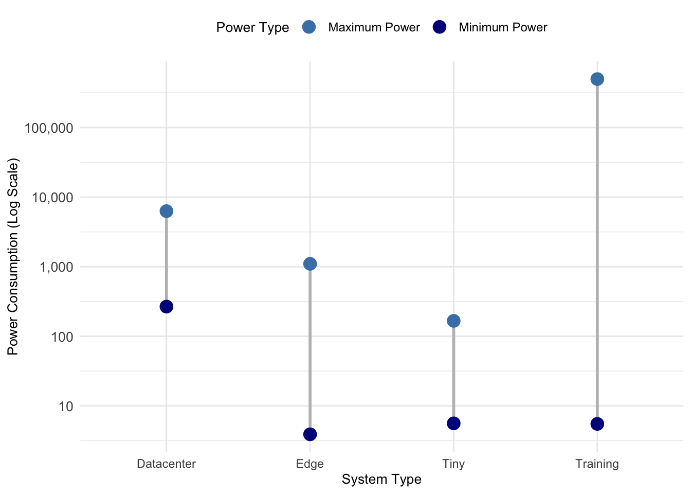](https://mlsysbook.ai/contents/core/benchmarking/benchmarking_files/figure-html/fig-power-differentials-1.png "Figure 7: Energy Consumption: The figure emphasizes the significant differences in power usage across various system types, from microwatts to megawatts, emphasizing the trade-offs between latency, cost, and energy efficiency in inference benchmarks.")
Figure 7: **Energy Consumption**: The figure emphasizes the significant differences in power usage across various system types, from microwatts to megawatts, emphasizing the trade-offs between latency, cost, and energy efficiency in inference benchmarks.
As with training, we will reference MLPerf Inference throughout this section to illustrate benchmarking principles. MLPerf’s inference benchmarks, building on the foundation established in [Section 1.2](https://mlsysbook.ai/contents/core/benchmarking/benchmarking.html#sec-benchmarking-ai-historical-context-1c54)
, provide standardized evaluation across deployment scenarios from cloud to edge devices.
### Inference Benchmark Motivation
Deploying machine learning models for inference introduces a unique set of challenges distinct from training. While training optimizes large-scale computation over extensive datasets, inference must deliver predictions efficiently and at scale in real-world environments. Inference benchmarks evaluate deployment-specific performance challenges, identifying bottlenecks that emerge when models transition from development to production serving.
Unlike training, which typically runs on dedicated high-performance hardware, inference must adapt to varying constraints. A model deployed in a cloud server might prioritize high-throughput batch processing, while the same model running on a mobile device must operate under strict latency and power constraints. On edge devices with limited compute and memory, model optimization techniques become critical. Benchmarks help assess these trade-offs, ensuring that inference systems maintain the right balance between accuracy, speed, and efficiency across different platforms.
Inference benchmarks help answer essential questions about model deployment. How quickly can a model generate predictions in real-world conditions? What are the trade-offs between inference speed and accuracy? Can an inference system handle increasing demand while maintaining low latency? By evaluating these factors, benchmarks guide optimizations in both hardware and software to improve overall efficiency ([Reddi et al. 2019](https://mlsysbook.ai/contents/core/benchmarking/benchmarking.html#ref-reddi2020mlperf)
).
#### Importance of Inference Benchmarks
Inference plays a critical role in AI applications, where performance directly affects usability and cost. Unlike training, which is often performed offline, inference typically operates in real-time or near real-time, making latency a primary concern. A self-driving car processing camera feeds must react within milliseconds, while a voice assistant generating responses should feel instantaneous to users.
Different applications impose varying constraints on inference. Some workloads require single-instance inference, where predictions must be made as quickly as possible for each individual input. This is crucial in real-time systems such as robotics, augmented reality, and conversational AI, where even small delays can impact responsiveness. Other workloads, such as large-scale recommendation systems or search engines, process massive batches of queries simultaneously, prioritizing throughput over per-query latency. Benchmarks allow engineers to evaluate both scenarios and ensure models are optimized for their intended use case.
A key difference between training and inference is that inference workloads often run continuously in production, meaning that small inefficiencies can compound over time. Unlike a training job that runs once and completes, an inference system deployed in the cloud may serve millions of queries daily, and a model running on a smartphone must manage battery consumption over extended use. Benchmarks provide a structured way to measure inference efficiency under these real-world constraints, helping developers make informed choices about model optimization, hardware selection, and deployment strategies.
#### Hardware & Software Optimization
Efficient inference depends on both hardware acceleration and software optimizations. While GPUs and TPUs dominate training, inference is more diverse in its hardware needs. A cloud-based AI service might leverage powerful accelerators for large-scale workloads, whereas mobile devices rely on specialized inference chips like NPUs or optimized CPU execution. On embedded systems, where resources are constrained, achieving high performance requires careful memory and compute efficiency. Benchmarks help evaluate how well different hardware platforms handle inference workloads, guiding deployment decisions.
Software optimizations are just as important. Frameworks like TensorRT[35](https://mlsysbook.ai/contents/core/benchmarking/benchmarking.html#fn35)
, ONNX Runtime[36](https://mlsysbook.ai/contents/core/benchmarking/benchmarking.html#fn36)
, and TVM[37](https://mlsysbook.ai/contents/core/benchmarking/benchmarking.html#fn37)
apply optimizations such as operator fusion[38](https://mlsysbook.ai/contents/core/benchmarking/benchmarking.html#fn38)
, numerical precision adjustments, and kernel tuning to improve inference speed and reduce computational overhead. These optimizations can make a significant difference, especially in environments with limited resources. Benchmarks allow developers to measure the impact of such techniques on latency, throughput, and power efficiency, ensuring that optimizations translate into real-world improvements without degrading model accuracy.
35 **TensorRT**: NVIDIA’s high-performance inference optimizer and runtime library that accelerates deep learning models on NVIDIA GPUs. Introduced in 2016, TensorRT applies graph optimizations, kernel fusion, and precision calibration to achieve 1.5-7x speedups over naive implementations, supporting FP16, INT8, and sparse matrix operations.
36 **ONNX Runtime**: Microsoft’s cross-platform, high-performance ML inferencing and training accelerator supporting the Open Neural Network Exchange (ONNX) format. Released in 2018, it enables models trained in any framework to run efficiently across different hardware (CPU, GPU, NPU) with optimizations like graph fusion and memory pattern optimization.
37 **TVM**: An open-source deep learning compiler stack that optimizes tensor programs for diverse hardware backends including CPUs, GPUs, and specialized accelerators. Developed at the University of Washington, TVM uses machine learning to automatically generate optimized code, achieving performance competitive with hand-tuned libraries while supporting new hardware architectures.
38 **Operator Fusion**: A compiler optimization technique that combines multiple neural network operations into single kernels to reduce memory bandwidth requirements and improve cache efficiency. For example, fusing convolution with batch normalization and ReLU can eliminate intermediate memory writes, achieving 20-40% speedups in inference workloads.
#### Scalability & Efficiency
Inference workloads vary significantly in their scaling requirements. A cloud-based AI system handling millions of queries per second must ensure that increasing demand does not cause delays, while a mobile application running a model locally must execute quickly even under power constraints. Unlike training, which is typically performed on a fixed set of high-performance machines, inference must scale dynamically based on usage patterns and available computational resources.
Benchmarks evaluate how inference systems scale under different conditions. They measure how well performance holds up under increasing query loads, whether additional compute resources improve inference speed, and how efficiently models run across different deployment environments. Large-scale inference deployments often involve distributed inference servers, where multiple copies of a model process incoming requests in parallel. Benchmarks assess how efficiently this scaling occurs and whether additional resources lead to meaningful improvements in latency and throughput.
Another key factor in inference efficiency is cold-start performance, the time it takes for a model to load and begin processing queries. This is especially relevant for applications that do not run inference continuously but instead load models on demand. Benchmarks help determine whether a system can quickly transition from idle to active execution without significant overhead.
#### Cost & Energy Factors
Because inference workloads run continuously, operational cost and energy efficiency are critical factors. Unlike training, where compute costs are incurred once, inference costs accumulate over time as models are deployed in production. Running an inefficient model at scale can significantly increase cloud compute expenses, while an inefficient mobile inference system can drain battery life quickly. Benchmarks provide insights into cost per inference request, helping organizations optimize for both performance and affordability.
Energy efficiency is also a growing concern, particularly for mobile and edge AI applications. Many inference workloads run on battery-powered devices, where excessive computation can impact usability. A model running on a smartphone, for example, must be optimized to minimize power consumption while maintaining responsiveness. Benchmarks help evaluate inference efficiency per watt, ensuring that models can operate sustainably across different platforms.
#### Fair ML Systems Comparison
Applying the standardized evaluation principles established for training benchmarks, inference evaluation requires the same rigorous comparison methodologies. MLPerf Inference extends these principles to deployment scenarios, defining evaluation criteria for tasks such as image classification, object detection, and speech recognition across different hardware platforms and optimization techniques. This ensures that inference performance comparisons remain meaningful and reproducible while accounting for deployment-specific constraints like latency requirements and energy efficiency.
### Inference Metrics
Evaluating the performance of inference systems requires a distinct set of metrics from those used for training. While training benchmarks emphasize throughput, scalability, and time-to-accuracy, inference benchmarks must focus on latency, efficiency, and resource utilization in practical deployment settings. These metrics ensure that machine learning models perform well across different environments, from cloud data centers handling millions of requests to mobile and edge devices operating under strict power and memory constraints.
Unlike training benchmarks that emphasize throughput and time-to-accuracy as established earlier, inference benchmarks evaluate how efficiently a trained model can process inputs and generate predictions at scale. The following sections describe the most important inference benchmarking metrics, explaining their relevance and how they are used to compare different systems.
#### Latency & Tail Latency
Latency is one of the most critical performance metrics for inference, particularly in real-time applications where delays can negatively impact user experience or system safety. Latency refers to the time taken for an inference system to process an input and produce a prediction. While the average latency of a system is useful, it does not capture performance in high-demand scenarios where occasional delays can degrade reliability.
To account for this, benchmarks often measure tail latency[39](https://mlsysbook.ai/contents/core/benchmarking/benchmarking.html#fn39)
, which reflects the worst-case delays in a system. These are typically reported as the 95th percentile (p95) or 99th percentile (p99) latency, meaning that 95% or 99% of inferences are completed within a given time. For applications such as autonomous driving or real-time trading, maintaining low tail latency is essential to avoid unpredictable delays that could lead to catastrophic outcomes.
39 **Tail Latency**: The worst-case response times (typically 95th or 99th percentile) that determine user experience in production systems. While average latency might be 50ms, 99th percentile could be 500ms due to garbage collection, thermal throttling, or resource contention. Production SLAs are set based on tail latency, not averages.
Tail latency’s connection to user experience at scale becomes critical in production systems serving millions of users. Even small P99 latency degradations create compounding effects across large user bases: if 1% of requests experience 10x latency (e.g., 1000ms instead of 100ms), this affects 10,000 users per million requests, potentially leading to timeout errors, poor user experience, and customer churn. Search engines and recommendation systems demonstrate this sensitivity: Google found that 500ms additional latency reduces search traffic by 20%, while Amazon discovered that 100ms latency increase decreases sales by 1%.
Service level objectives (SLOs) in production systems therefore focus on tail latency rather than mean latency to ensure consistent user experience. Typical production SLOs specify P95 < 100ms and P99 < 500ms for interactive services, recognizing that occasional slow responses have disproportionate impact on user satisfaction. Large-scale systems like Netflix and Uber optimize for P99.9 latency to handle traffic spikes and infrastructure variations that affect service reliability.
#### Throughput & Batch Efficiency
While latency measures the speed of individual inference requests, throughput measures how many inference requests a system can process per second. It is typically expressed in queries per second (QPS) or frames per second (FPS) for vision tasks. Some inference systems operate on a single-instance basis, where each input is processed independently as soon as it arrives. Other systems process multiple inputs in parallel using batch inference, which can significantly improve efficiency by leveraging hardware optimizations.
For example, cloud-based services handling millions of queries per second benefit from batch inference, where large groups of inputs are processed together to maximize computational efficiency. In contrast, applications like robotics, interactive AI, and augmented reality require low-latency single-instance inference, where the system must respond immediately to each new input.
Benchmarks must consider both single-instance and batch throughput to provide a comprehensive understanding of inference performance across different deployment scenarios.
#### Precision & Accuracy Trade-offs
Optimizing inference performance often involves reducing numerical precision, which can significantly accelerate computation while reducing memory and energy consumption. However, lower-precision calculations can introduce accuracy degradation, making it essential to benchmark the trade-offs between speed and predictive quality.
Inference benchmarks evaluate how well models perform under different numerical settings, such as FP32[40](https://mlsysbook.ai/contents/core/benchmarking/benchmarking.html#fn40)
, FP16[41](https://mlsysbook.ai/contents/core/benchmarking/benchmarking.html#fn41)
, and INT8[42](https://mlsysbook.ai/contents/core/benchmarking/benchmarking.html#fn42)
. Many modern AI accelerators support mixed-precision inference, allowing systems to dynamically adjust numerical representation based on workload requirements. Model compression techniques[43](https://mlsysbook.ai/contents/core/benchmarking/benchmarking.html#fn43)
further improve efficiency, but their impact on model accuracy varies depending on the task and dataset. Benchmarks help determine whether these optimizations are viable for deployment, ensuring that improvements in efficiency do not come at the cost of unacceptable accuracy loss.
40 **FP32**: 32-bit floating-point format providing high numerical precision with approximately 7 decimal digits of accuracy. Standard for research and training, FP32 operations consume maximum memory and computational resources but ensure numerical stability. Modern GPUs achieve 15-20 TFLOPS in FP32, serving as the baseline for precision comparisons.
41 **FP16**: 16-bit floating-point format that halves memory usage compared to FP32 while maintaining reasonable numerical precision. Widely supported by modern AI accelerators, FP16 can achieve 2-4x speedups over FP32 with minimal accuracy loss for most deep learning models, making it the preferred format for inference and mixed-precision training.
42 **INT8**: 8-bit integer format providing maximum memory and computational efficiency, requiring only 25% of FP32 storage. Post-training precision reduction to INT8 can achieve 4x memory reduction and 2-4x speedup on specialized hardware, but requires careful calibration to minimize accuracy degradation, typically maintaining 95-99% of original model performance.
43 **Model Compression**: Techniques to reduce model size and computational requirements including precision reduction (reducing numerical precision), structural optimization (removing unnecessary parameters), knowledge transfer (training smaller models to mimic larger ones), and tensor decomposition. These methods can achieve 10-100x size reduction while maintaining 90-99% of original accuracy.
#### Memory Footprint & Model Size
Beyond computational optimizations, memory footprint is another critical consideration for inference systems, particularly for devices with limited resources. Efficient inference depends not only on speed but also on memory usage. Unlike training, where large models can be distributed across powerful GPUs or TPUs, inference often requires models to run within strict memory budgets. The total model size determines how much storage is required for deployment, while RAM usage reflects the working memory needed during execution. Some models require large memory bandwidth to efficiently transfer data between processing units, which can become a bottleneck if the hardware lacks sufficient capacity.
Inference benchmarks evaluate these factors to ensure that models can be deployed effectively across a range of devices. A model that achieves high accuracy but exceeds memory constraints may be impractical for real-world use. To address this, various compression techniques are often applied to reduce model size while maintaining accuracy. Benchmarks help assess whether these optimizations strike the right balance between memory efficiency and predictive performance.
#### Cold-Start & Model Load Time
Once memory requirements are optimized, cold-start performance becomes critical for ensuring inference systems are ready to respond quickly upon deployment. In many deployment scenarios, models are not always kept in memory but instead loaded on demand when needed. This can introduce significant delays, particularly in serverless AI environments[44](https://mlsysbook.ai/contents/core/benchmarking/benchmarking.html#fn44)
, where resources are allocated dynamically based on incoming requests. Cold-start performance measures how quickly a system can transition from idle to active execution, ensuring that inference is available without excessive wait times.
44 **Serverless AI**: Cloud computing paradigm where ML models are deployed as functions that automatically scale from zero to handle incoming requests, with users paying only for actual inference time. Popular platforms like AWS Lambda, Google Cloud Functions, and Azure Functions support serverless AI, but cold-start latencies of 1-10 seconds for large models can impact user experience compared to always-on deployments.
Model load time refers to the duration required to load a trained model into memory before it can process inputs. In some cases, particularly on resource-limited devices, models must be reloaded frequently to free up memory for other applications. The time taken for the first inference request is also an important consideration, as it reflects the total delay users experience when interacting with an AI-powered service. Benchmarks help quantify these delays, ensuring that inference systems can meet real-world responsiveness requirements.
#### Dynamic Workload Scaling
While cold-start latency addresses initial responsiveness, scalability ensures that inference systems can handle fluctuating workloads and concurrent demands over time Inference workloads must scale effectively across different usage patterns. In cloud-based AI services, this means efficiently handling millions of concurrent users, while on mobile or embedded devices, it involves managing multiple AI models running simultaneously without overloading the system.
Scalability measures how well inference performance improves when additional computational resources are allocated. In some cases, adding more GPUs or TPUs increases throughput significantly, but in other scenarios, bottlenecks such as memory bandwidth limitations or network latency may limit scaling efficiency. Benchmarks also assess how well a system balances multiple concurrent models in real-world deployment, where different AI-powered features may need to run at the same time without interference.
For cloud-based AI, benchmarks evaluate how efficiently a system handles fluctuating demand, ensuring that inference servers can dynamically allocate resources without compromising latency. In mobile and embedded AI, efficient multi-model execution is essential for running multiple AI-powered features simultaneously without degrading system performance.
#### Energy Consumption & Efficiency
Since inference workloads run continuously in production, power consumption and energy efficiency are critical considerations. This is particularly important for mobile and edge devices, where battery life and thermal constraints limit available computational resources. Even in large-scale cloud environments, power efficiency directly impacts operational costs and sustainability goals.
The energy required for a single inference is often measured in joules per inference, reflecting how efficiently a system processes inputs while minimizing power draw. In cloud-based inference, efficiency is commonly expressed as queries per second per watt (QPS/W) to quantify how well a system balances performance and energy consumption. For mobile AI applications, optimizing inference power consumption extends battery life and allows models to run efficiently on resource-constrained devices. Reducing energy use also plays a key role in making large-scale AI systems more environmentally sustainable, ensuring that computational advancements align with energy-conscious deployment strategies. By balancing power consumption with performance, energy-efficient inference systems enable AI to scale sustainably across diverse applications, from data centers to edge devices.
### Inference Performance Evaluation
Evaluating inference performance is a critical step in understanding how well machine learning systems meet the demands of real-world applications. Unlike training, which is typically conducted offline, inference systems must process inputs and generate predictions efficiently across a wide range of deployment scenarios. Metrics such as latency, throughput, memory usage, and energy efficiency provide a structured way to measure system performance and identify areas for improvement.
[Table 3](https://mlsysbook.ai/contents/core/benchmarking/benchmarking.html#tbl-inference-metrics)
below summarizes the key metrics used to evaluate inference systems, highlighting their relevance to different contexts. While each metric offers unique insights, it is important to approach inference benchmarking holistically. Trade-offs between metrics, including speed versus accuracy and throughput versus power consumption, are common, and understanding these trade-offs is essential for effective system design.
Table 3: **Inference Performance Metrics**: Evaluating latency, throughput, and resource usage provides a quantitative basis for optimizing deployed machine learning systems and selecting appropriate hardware configurations. Understanding these metrics and the trade-offs between them is crucial for balancing speed, cost, and accuracy in real-world applications.
| | | |
| --- | --- | --- |
| **Latency and Tail Latency** | Mean latency (ms/request); Tail latency (p95, p99, p99.9) | Evaluating real-time performance for safety-critical AI |
| **Throughput and Efficiency** | Queries per second (QPS); Frames per second (FPS); Batch throughput | Comparing large-scale cloud inference systems |
| **Numerical Precision Impact** | Accuracy degradation (FP32 vs. INT8); Speedup from reduced precision | Balancing accuracy vs. efficiency in optimized inference |
| **Memory Footprint** | Model size (MB/GB); RAM usage (MB); Memory bandwidth utilization | Assessing feasibility for edge and mobile deployments |
| **Cold-Start and Load Time** | Model load time (s); First inference latency (s) | Evaluating responsiveness in serverless AI |
| **Scalability** | Efficiency under load; Multi-model serving performance | Measuring robustness for dynamic, high-demand systems |
| **Power and Energy Efficiency** | Power consumption (Watts); Performance per Watt (QPS/W) | Optimizing energy use for mobile and sustainable AI |
#### Inference Systems Considerations
Inference systems face unique challenges depending on where and how they are deployed. Real-time applications, such as self-driving cars or voice assistants, require low latency to ensure timely responses, while large-scale cloud deployments focus on maximizing throughput to handle millions of queries. Edge devices, on the other hand, are constrained by memory and power, making efficiency critical.
One of the most important aspects of evaluating inference performance is understanding the trade-offs between metrics. For example, optimizing for high throughput might increase latency, making a system unsuitable for real-time applications. Similarly, reducing numerical precision improves power efficiency and speed but may lead to minor accuracy degradation. A thoughtful evaluation must balance these trade-offs to align with the intended application.
The deployment environment also plays a significant role in determining evaluation priorities. Cloud-based systems often prioritize scalability and adaptability to dynamic workloads, while mobile and edge systems require careful attention to memory usage and energy efficiency. These differing priorities mean that benchmarks must be tailored to the context of the system’s use, rather than relying on one-size-fits-all evaluations.
Ultimately, evaluating inference performance requires a holistic approach. Focusing on a single metric, such as latency or energy efficiency, provides an incomplete picture. Instead, all relevant dimensions must be considered together to ensure that the system meets its functional, resource, and performance goals in a balanced way.
#### Context-Dependent Metrics
Different deployment scenarios require distinctly different metric priorities, as the operational constraints and success criteria vary dramatically across contexts. Understanding these priorities allows engineers to focus benchmarking efforts effectively and interpret results within appropriate decision frameworks. [Table 4](https://mlsysbook.ai/contents/core/benchmarking/benchmarking.html#tbl-metric-priorities)
illustrates how performance priorities shift across five major deployment contexts, revealing the systematic relationship between operational constraints and optimization targets.
Table 4: **Performance Metric Priorities by Deployment Context**: Different operational environments demand distinct optimization focuses, reflecting varying constraints and success criteria. Understanding these priorities guides both benchmark selection and result interpretation within appropriate decision frameworks.
| | | | | |
| --- | --- | --- | --- | --- |
| **Real-Time Applications** | Latency (p95 < 50ms) | Reliability (99.9%) | Memory Footprint | User experience demands immediate response |
| **Cloud-Scale Services** | Throughput (QPS) | Cost Efficiency | Average Latency | Business viability requires massive scale |
| **Edge/Mobile Devices** | Power Consumption | Memory Footprint | Latency | Battery life and resource limits dominate |
| **Training Workloads** | Training Time | GPU Utilization | Memory Efficiency | Research velocity enables faster experimentation |
| **Scientific/Medical** | Accuracy | Reliability | Explainability | Correctness cannot be compromised for performance |
The hierarchy shown in [Table 4](https://mlsysbook.ai/contents/core/benchmarking/benchmarking.html#tbl-metric-priorities)
reflects how operational constraints drive performance optimization strategies. Real-time applications exemplify latency-critical deployments where user experience depends on immediate system response. Autonomous vehicle perception systems must process sensor data within strict timing deadlines, making p95 latency more important than peak throughput. The table shows reliability as the secondary priority because system failures in autonomous vehicles carry safety implications that transcend performance concerns.
Conversely, cloud-scale services prioritize aggregate throughput to handle millions of concurrent users, accepting higher average latency in exchange for improved cost efficiency per query. The progression from throughput to cost efficiency to latency reflects economic realities: cloud providers must optimize for revenue per server while maintaining acceptable user experience. Notice how the same metric (latency) ranks as primary for real-time applications but tertiary for cloud services, demonstrating the context-dependent nature of performance evaluation.
Edge and mobile deployments face distinctly different constraints, where battery life and thermal limitations dominate design decisions. A smartphone AI assistant that improves throughput by 50% but increases power consumption by 30% represents a net regression, as reduced battery life directly impacts user satisfaction. Training workloads present another distinct optimization landscape, where research productivity depends on experiment turnaround time, making GPU utilization efficiency and memory bandwidth critical for enabling larger model exploration.
Scientific and medical applications establish accuracy and reliability as non-negotiable requirements, with performance optimization serving these primary objectives rather than substituting for them. A medical diagnostic system achieving 99.2% accuracy at 10ms latency provides superior value compared to 98.8% accuracy at 5ms latency, demonstrating how context-specific priorities guide meaningful performance evaluation.
This prioritization framework fundamentally shapes benchmark interpretation and optimization strategies. Achieving 2x throughput improvement represents significant value for cloud deployments but provides minimal benefit for battery-powered edge devices where 20% power reduction delivers superior operational impact.
#### Inference Benchmark Pitfalls
Even with well-defined metrics, benchmarking inference systems can be challenging. Missteps during the evaluation process often lead to misleading conclusions. Below are common pitfalls that students and practitioners should be aware of when analyzing inference performance.
##### Overemphasis on Average Latency
While average latency provides a baseline measure of response time, it fails to capture how a system performs under peak load. In real-world scenarios, worst-case latency, which is captured through metrics such as p95[45](https://mlsysbook.ai/contents/core/benchmarking/benchmarking.html#fn45)
or p99[46](https://mlsysbook.ai/contents/core/benchmarking/benchmarking.html#fn46)
tail latency, can significantly impact system reliability. For instance, a conversational AI system may fail to provide timely responses if occasional latency spikes exceed acceptable thresholds.
45 **P95 Latency**: The 95th percentile latency measurement, meaning 95% of requests complete within this time while 5% take longer. For example, if p95 latency is 100ms, then 19 out of 20 requests finish within 100ms. P95 is widely used in SLA agreements because it captures typical user experience while acknowledging that some requests will naturally take longer due to system variability.
46 **P99 Latency**: The 99th percentile latency measurement, indicating that 99% of requests complete within this time while only 1% experience longer delays. P99 latency is crucial for user-facing applications where even rare slow responses significantly impact user satisfaction. For instance, if a web service handles 1 million requests daily, p99 latency determines the experience for 10,000 users.
##### Ignoring Memory & Energy Constraints
A model with excellent throughput or latency may be unsuitable for mobile or edge deployments if it requires excessive memory or power. For example, an inference system designed for cloud environments might fail to operate efficiently on a battery-powered device. Proper benchmarks must consider memory footprint and energy consumption to ensure practicality across deployment contexts.
##### Ignoring Cold-Start Performance
In serverless environments, where models are loaded on demand, cold-start latency[47](https://mlsysbook.ai/contents/core/benchmarking/benchmarking.html#fn47)
is a critical factor. Ignoring the time it takes to initialize a model and process the first request can result in unrealistic expectations for responsiveness. Evaluating both model load time and first-inference latency ensures that systems are designed to meet real-world responsiveness requirements.
47 **Cold-Start Latency**: The initialization time required when a system or service starts from a completely idle state, including time to load libraries, initialize models, and allocate memory. In serverless AI deployments, cold-start latencies range from 100ms for simple models to 10+ seconds for large language models, significantly impacting user experience compared to warm instances that respond in milliseconds.
##### Isolated Metrics Evaluation
Benchmarking inference systems often involves balancing competing metrics. For example, maximizing batch throughput might degrade latency, while aggressive precision reduction could reduce accuracy. Focusing on a single metric without considering its impact on others can lead to incomplete or misleading evaluations.
Numerical precision optimization exemplifies this challenge particularly well. Individual accelerator benchmarks show INT8 operations achieving 4x higher TOPS[48](https://mlsysbook.ai/contents/core/benchmarking/benchmarking.html#fn48)
(Tera Operations Per Second) compared to FP32, creating compelling performance narratives.
48 **TOPS (Tera Operations Per Second)**: A measure of computational throughput indicating trillions of operations per second, commonly used for AI accelerator performance. Modern AI chips achieve 100-1000 TOPS for INT8 operations: NVIDIA H100 delivers 2000 TOPS INT8, Apple M2 Neural Engine provides 15.8 TOPS, while edge devices like Google Edge TPU achieve 4 TOPS. Higher TOPS enable faster AI inference and training. However, when these accelerators deploy in complete training systems, the chip-level advantage often disappears due to increased convergence time, precision conversion overhead, and mixed-precision coordination complexity. The “4x faster” micro-benchmark translates into slower end-to-end training, demonstrating why isolated hardware metrics cannot substitute for holistic system evaluation. Balanced approaches like FP16 mixed-precision often provide superior system-level performance despite lower peak TOPS measurements. Comprehensive benchmarks must account for these cross-metric interactions and system-level complexities.
##### Linear Scaling Assumption
Inference performance does not always scale proportionally with additional resources. Bottlenecks such as memory bandwidth, thermal limits, or communication overhead can limit the benefits of adding more GPUs or TPUs. As discussed in **[Chapter 11: AI Acceleration](https://mlsysbook.ai/contents/core/hw_acceleration/hw_acceleration.html#sec-ai-acceleration)
**, these scaling limitations arise from fundamental hardware constraints and interconnect architectures. Benchmarks that assume linear scaling behavior may overestimate system performance, particularly in distributed deployments.
##### Ignoring Application Requirements
Generic benchmarking results may fail to account for the specific needs of an application. For instance, a benchmark optimized for cloud inference might be irrelevant for edge devices, where energy and memory constraints dominate. Tailoring benchmarks to the deployment context ensures that results are meaningful and actionable.
##### Statistical Significance & Noise
Distinguishing meaningful performance improvements from measurement noise requires proper statistical analysis. Following the evaluation methodology principles established earlier, MLPerf addresses measurement variability by requiring multiple benchmark runs and reporting percentile-based metrics rather than single measurements ([Reddi et al. 2019](https://mlsysbook.ai/contents/core/benchmarking/benchmarking.html#ref-reddi2020mlperf)
). For instance, MLPerf Inference reports 99th percentile latency alongside mean performance, capturing both typical behavior and worst-case scenarios that single-run measurements might miss. This approach recognizes that system performance naturally varies due to factors like thermal throttling, memory allocation patterns, and background processes.
Reddi, Vijay Janapa, Christine Cheng, David Kanter, Peter Mattson, Guenther Schmuelling, Carole-Jean Wu, Brian Anderson, et al. 2019. “MLPerf Inference Benchmark.” _arXiv Preprint arXiv:1911.02549_, November, 446–59. [https://doi.org/10.1109/isca45697.2020.00045](https://doi.org/10.1109/isca45697.2020.00045)
.
#### Inference Benchmark Synthesis
Inference benchmarks are essential tools for understanding system performance, but their utility depends on careful and holistic evaluation. Metrics like latency, throughput, memory usage, and energy efficiency provide valuable insights, but their importance varies depending on the application and deployment context. Students should approach benchmarking as a process of balancing multiple priorities, rather than optimizing for a single metric.
Avoiding common pitfalls and considering the trade-offs between different metrics allows practitioners to design inference systems that are reliable, efficient, and suitable for real-world deployment. The ultimate goal of benchmarking is to guide system improvements that align with the demands of the intended application.
### MLPerf Inference Benchmarks
The MLPerf Inference benchmark, developed by MLCommons[49](https://mlsysbook.ai/contents/core/benchmarking/benchmarking.html#fn49)
, provides a standardized framework for evaluating machine learning inference performance across a range of deployment environments. Initially, MLPerf started with a single inference benchmark, but as machine learning systems expanded into diverse applications, it became clear that a one-size-fits-all benchmark was insufficient. Different inference scenarios, including cloud-based AI services and resource-constrained embedded devices, demanded tailored evaluations. This realization led to the development of a family of MLPerf inference benchmarks, each designed to assess performance within a specific deployment setting.
49 **MLCommons**: Non-profit organization founded in 2018 (originally MLPerf) to develop ML benchmarking standards. Governed by 40+ industry leaders including Google, NVIDIA, Intel, and Facebook, MLCommons has established the de facto standards for AI performance measurement across cloud to edge deployments.
#### MLPerf Inference
[MLPerf Inference](https://mlcommons.org/en/inference-datacenter/)
serves as the baseline benchmark, originally designed to evaluate large-scale inference systems. It primarily focuses on data center and cloud-based inference workloads, where high throughput, low latency, and efficient resource utilization are essential. The benchmark assesses performance across a range of deep learning models, including image classification, object detection, natural language processing, and recommendation systems. This version of MLPerf remains the gold standard for comparing AI accelerators, GPUs, TPUs, and CPUs in high-performance computing environments.
Major technology companies regularly reference MLPerf results for hardware procurement decisions. When evaluating hardware for recommendation systems infrastructure, MLPerf benchmark scores on DLRM[50](https://mlsysbook.ai/contents/core/benchmarking/benchmarking.html#fn50)
(Deep Learning Recommendation Model) workloads directly inform choices between different accelerator generations. Benchmarks consistently show that newer GPU architectures deliver 2-3x higher throughput on recommendation inference compared to previous generations, often justifying premium costs for production deployment at scale. This demonstrates how standardized benchmarks translate directly into multi-million dollar infrastructure decisions across the industry.
50 **DLRM (Deep Learning Recommendation Model)**: Facebook’s neural network architecture for personalized recommendations, released in 2019, combining categorical features through embedding tables with continuous features through multi-layer perceptrons. DLRM models can contain 100+ billion parameters with embedding tables consuming terabytes of memory, requiring specialized hardware optimization for the sparse matrix operations that dominate recommendation system workloads.
The Cost of Comprehensive Benchmarking
While benchmarking is essential for ML system development, it comes with substantial costs that limit participation to well-resourced organizations. Submitting to MLPerf can require significant engineering effort and hundreds of thousands of dollars in hardware and cloud compute time. A comprehensive MLPerf Training submission involves months of engineering time for optimization, tuning, and validation across multiple hardware configurations. The computational costs alone can exceed $100,000 for a full submission covering multiple workloads and system scales.
This cost barrier explains why MLPerf submissions are dominated by major technology companies and hardware vendors, while smaller organizations rely on published results rather than conducting their own comprehensive evaluations. The high barrier to entry motivates the need for more lightweight, internal benchmarking practices that organizations can use to make informed decisions without the expense of full-scale standardized benchmarking.
#### MLPerf Mobile
[MLPerf Mobile](https://mlcommons.org/en/mlperf-mobile/)
extends MLPerf’s evaluation framework to smartphones and other mobile devices. Unlike cloud-based inference, mobile inference operates under strict power and memory constraints, requiring models to be optimized for efficiency without sacrificing responsiveness. The benchmark measures latency and responsiveness for real-time AI tasks, such as camera-based scene detection, speech recognition, and augmented reality applications. MLPerf Mobile has become an industry standard for assessing AI performance on flagship smartphones and mobile AI chips, helping developers optimize models for on-device AI workloads.
#### MLPerf Client
[MLPerf Client](https://mlcommons.org/en/inference-edge/)
focuses on inference performance on consumer computing devices, such as laptops, desktops, and workstations. This benchmark addresses local AI workloads that run directly on personal devices, eliminating reliance on cloud inference. Tasks such as real-time video editing, speech-to-text transcription, and AI-enhanced productivity applications fall under this category. Unlike cloud-based benchmarks, MLPerf Client evaluates how AI workloads interact with general-purpose hardware, such as CPUs, discrete GPUs, and integrated Neural Processing Units (NPUs), making it relevant for consumer and enterprise AI applications.
#### MLPerf Tiny
[MLPerf Tiny](https://mlcommons.org/en/inference-tiny/)
was created to benchmark embedded and ultra-low-power AI systems, such as IoT devices, wearables, and microcontrollers. Unlike other MLPerf benchmarks, which assess performance on powerful accelerators, MLPerf Tiny evaluates inference on devices with limited compute, memory, and power resources. This benchmark is particularly relevant for applications such as smart sensors, AI-driven automation, and real-time industrial monitoring, where models must run efficiently on hardware with minimal processing capabilities. MLPerf Tiny plays a crucial role in the advancement of AI at the edge, helping developers optimize models for constrained environments.
#### Evolution and Future Directions
The evolution of MLPerf Inference from a single benchmark to a spectrum of benchmarks reflects the diversity of AI deployment scenarios. Different environments, including cloud, mobile, desktop, and embedded environments, have unique constraints and requirements, and MLPerf provides a structured way to evaluate AI models accordingly.
MLPerf is an essential tool for:
* Understanding how inference performance varies across deployment settings.
* Learning which performance metrics are most relevant for different AI applications.
* Optimizing models and hardware choices based on real-world usage constraints.
Recognizing the necessity of tailored inference benchmarks deepens our understanding of AI deployment challenges and highlights the importance of benchmarking in developing efficient, scalable, and practical machine learning systems.
Energy efficiency considerations are integrated throughout Training (Section 8.2) and Inference (Section 8.3) benchmark methodologies, recognizing that power consumption affects both phases differently. Training energy costs are amortized across model lifetime, while inference energy costs accumulate per query and directly impact operational efficiency. The following analysis of power measurement techniques supports the energy metrics covered within each benchmarking phase.
**Self-Check: Question 1.8**
1. Which of the following metrics is most critical for evaluating real-time inference performance?
1. Tail Latency
2. Mean Latency
3. Throughput
4. Memory Footprint
2. Explain why precision optimization techniques are important in inference benchmarks and what trade-offs they might involve.
3. True or False: Inference benchmarks primarily focus on the training phase of machine learning models.
4. Order the following factors in terms of their impact on inference efficiency: (1) Model architecture, (2) Hardware configuration, (3) Precision optimization.
5. What is a key consideration when deploying inference systems on edge devices?
1. Maximizing throughput
2. Maximizing model size
3. Minimizing power consumption
4. Minimizing training time
[See Answers →](https://mlsysbook.ai/contents/core/benchmarking/benchmarking.html#quiz-answer-sec-benchmarking-ai-inference-benchmarks-433b)
Power Measurement Techniques
----------------------------
Energy efficiency benchmarking requires specialized measurement techniques that account for the diverse power scales across ML deployment environments. Building upon energy considerations established in training and inference sections, these techniques enable systematic validation of optimization claims from **[Chapter 10: Model Optimizations](https://mlsysbook.ai/contents/core/optimizations/optimizations.html#sec-model-optimizations)
** and hardware efficiency improvements from **[Chapter 11: AI Acceleration](https://mlsysbook.ai/contents/core/hw_acceleration/hw_acceleration.html#sec-ai-acceleration)
**.
While performance benchmarks help optimize speed and accuracy, they do not always account for energy efficiency, which has become an increasingly critical factor in real-world deployment. The energy efficiency principles from **[Chapter 9: Efficient AI](https://mlsysbook.ai/contents/core/efficient_ai/efficient_ai.html#sec-efficient-ai)
**, balancing computational complexity, memory access patterns, and hardware utilization, require quantitative validation through standardized energy benchmarks. These benchmarks enable us to verify whether architectural optimizations from **[Chapter 10: Model Optimizations](https://mlsysbook.ai/contents/core/optimizations/optimizations.html#sec-model-optimizations)
** and hardware-aware designs from **[Chapter 11: AI Acceleration](https://mlsysbook.ai/contents/core/hw_acceleration/hw_acceleration.html#sec-ai-acceleration)
** actually deliver promised energy savings in practice.
However, measuring power consumption in machine learning systems presents fundamentally unique challenges. The energy demands of ML models vary dramatically across deployment environments, spanning multiple orders of magnitude as shown in [Table 5](https://mlsysbook.ai/contents/core/benchmarking/benchmarking.html#tbl-power)
. This wide spectrum, spanning from TinyML devices consuming mere microwatts to data center racks requiring kilowatts, illustrates the fundamental challenge in creating standardized benchmarking methodologies ([Henderson et al. 2020](https://mlsysbook.ai/contents/core/benchmarking/benchmarking.html#ref-henderson2020towards)
).
Henderson, Peter, Jieru Hu, Joshua Romoff, Emma Brunskill, Dan Jurafsky, and Joelle Pineau. 2020. “Towards the Systematic Reporting of the Energy and Carbon Footprints of Machine Learning.” _CoRR_ abs/2002.05651 (248): 1–43. [https://doi.org/10.48550/arxiv.2002.05651](https://doi.org/10.48550/arxiv.2002.05651)
.
Table 5: **Power Consumption Spectrum**: Machine learning deployments exhibit a wide range of power demands, from microwatt-scale TinyML devices to milliwatt-scale microcontrollers; this variability challenges the development of standardized energy efficiency benchmarks. Understanding these differences is crucial for optimizing model deployment across resource-constrained and high-performance computing environments.
| | | |
| --- | --- | --- |
| **Tiny** | Neural Decision Processor (NDP) | 150 µW |
| **Tiny** | M7 Microcontroller | 25 mW |
| **Mobile** | Raspberry Pi 4 | 3.5 W |
| **Mobile** | Smartphone | 4 W |
| **Edge** | Smart Camera | 10-15 W |
| **Edge** | Edge Server | 65-95 W |
| **Cloud** | ML Server Node | 300-500 W |
| **Cloud** | ML Server Rack | 4-10 kW |
This dramatic range in power requirements, which spans over four orders of magnitude, presents significant challenges for measurement and benchmarking. Consequently, creating a unified methodology requires careful consideration of each scale’s unique characteristics. For example, accurately measuring microwatt-level consumption in TinyML devices demands different instrumentation and techniques than monitoring kilowatt-scale server racks. Any comprehensive benchmarking framework must accommodate these vastly different scales while ensuring measurements remain consistent, fair, and reproducible across diverse hardware configurations.
### Power Measurement Boundaries
To address these measurement challenges, [Figure 8](https://mlsysbook.ai/contents/core/benchmarking/benchmarking.html#fig-power-diagram)
illustrates how power consumption is measured at different system scales, from TinyML devices to full-scale data center inference nodes. Each scenario highlights distinct measurement boundaries, shown in green, which indicate the components included in energy accounting. Components outside these boundaries, shown with red dashed outlines, are excluded from power measurements.
[](https://mlsysbook.ai/contents/core/benchmarking/5fc9fcd7ee5d5add57deb446f637cb84d8f9b7dc.svg "Figure 8: Power Measurement Boundaries: MLPerf defines system boundaries for power measurement, ranging from single-chip devices to full data center nodes, to enable fair comparisons of energy efficiency across diverse hardware platforms. these boundaries delineate which components’ power consumption is included in reported metrics, impacting the interpretation of performance results. Source: [@tschand2024mlperf].")
Figure 8: **Power Measurement Boundaries**: MLPerf defines system boundaries for power measurement, ranging from single-chip devices to full data center nodes, to enable fair comparisons of energy efficiency across diverse hardware platforms. these boundaries delineate which components’ power consumption is included in reported metrics, impacting the interpretation of performance results. Source: ([Tschand et al. 2024](https://mlsysbook.ai/contents/core/benchmarking/benchmarking.html#ref-tschand2024mlperf)
).
The diagram is organized into three categories, Tiny, Inference, and Training examples, each reflecting different measurement scopes based on system architecture and deployment environment. In TinyML systems, the entire low-power SoC, including compute, memory, and basic interconnects, typically falls within the measurement boundary. Inference nodes introduce more complexity, incorporating multiple SoCs, local storage, accelerators, and memory, while often excluding remote storage and off-chip components. Training deployments span multiple racks, where only selected elements, including compute nodes and network switches, are measured, while storage systems, cooling infrastructure, and parts of the interconnect fabric are often excluded.
System-level power measurement offers a more holistic view than measuring individual components in isolation. While component-level metrics (e.g., accelerator or processor power) are valuable for performance tuning, real-world ML workloads involve intricate interactions between compute units, memory systems, and supporting infrastructure. For instance, analysis of Google’s TensorFlow Mobile workloads shows that data movement accounts for 57.3% of total inference energy consumption ([Boroumand et al. 2018](https://mlsysbook.ai/contents/core/benchmarking/benchmarking.html#ref-BoroumandASPLOS2018)
), highlighting how memory-bound operations can dominate system power usage.
Boroumand, Amirali, Saugata Ghose, Youngsok Kim, Rachata Ausavarungnirun, Eric Shiu, Rahul Thakur, Daehyun Kim, et al. 2018. “Google Workloads for Consumer Devices: Mitigating Data Movement Bottlenecks.” In _Proceedings of the Twenty-Third International Conference on Architectural Support for Programming Languages and Operating Systems_, 316–31. ASPLOS ’18. ACM. [https://doi.org/10.1145/3173162.3173177](https://doi.org/10.1145/3173162.3173177)
.
Barroso, Luiz André, Jimmy Clidaras, and Urs Hölzle. 2013. _The Datacenter as a Computer: An Introduction to the Design of Warehouse-Scale Machines_. Springer International Publishing. [https://doi.org/10.1007/978-3-031-01741-4](https://doi.org/10.1007/978-3-031-01741-4)
.
Shared infrastructure presents additional challenges. In data centers, resources such as cooling systems and power delivery are shared across workloads, complicating attribution of energy use to specific ML tasks. Cooling alone can account for 20-30% of total facility power consumption, making it a major factor in energy efficiency assessments ([Barroso, Clidaras, and Hölzle 2013](https://mlsysbook.ai/contents/core/benchmarking/benchmarking.html#ref-barroso2022datacenter)
). Even at the edge, components like memory and I/O interfaces may serve both ML and non-ML functions, further blurring measurement boundaries.
Shared infrastructure complexity is further compounded by dynamic power management techniques that modern systems employ to optimize energy efficiency. Dynamic voltage and frequency scaling (DVFS) adjusts processor voltage and clock frequency based on workload demands, enabling significant power reductions during periods of lower computational intensity. Advanced DVFS implementations using on-chip switching regulators can achieve substantial energy savings ([Kim et al. 2008](https://mlsysbook.ai/contents/core/benchmarking/benchmarking.html#ref-kim2008system)
), causing power consumption to vary by 30-50% for the same ML model depending on system load and concurrent activity. This variability affects not only the compute components but also the supporting infrastructure, as reduced processor activity can lower cooling requirements and overall facility power draw.
Kim, Wonyoung, Meeta S. Gupta, Gu-Yeon Wei, and David Brooks. 2008. “System Level Analysis of Fast, Per-Core DVFS Using on-Chip Switching Regulators.” In _2008 IEEE 14th International Symposium on High Performance Computer Architecture_, 123–34. HPCA ’08. IEEE. [https://doi.org/10.1109/hpca.2008.4658633](https://doi.org/10.1109/hpca.2008.4658633)
.
Barroso, Luiz André, Urs Hölzle, and Parthasarathy Ranganathan. 2019. _The Datacenter as a Computer: Designing Warehouse-Scale Machines_. Springer International Publishing. [https://doi.org/10.1007/978-3-031-01761-2](https://doi.org/10.1007/978-3-031-01761-2)
.
Support infrastructure, particularly cooling systems, is a major component of total energy consumption in large-scale deployments. Data centers must maintain operational temperatures, typically between 20-25°C, to ensure system reliability. Cooling overhead is captured in the Power Usage Effectiveness (PUE) metric, which ranges from 1.1 in highly efficient facilities to over 2.0 in less optimized ones ([Barroso, Hölzle, and Ranganathan 2019](https://mlsysbook.ai/contents/core/benchmarking/benchmarking.html#ref-barroso2019datacenter)
). The interaction between compute workloads and cooling infrastructure creates complex dependencies; for example, power management techniques like DVFS not only reduce direct processor power consumption but also decrease heat generation, creating cascading effects on cooling requirements. Even edge devices require basic thermal management.
### Computational Efficiency vs. Power Consumption
The relationship between computational performance and energy efficiency is one of the most important tradeoffs in modern ML system design. As systems push for higher performance, they often encounter diminishing returns in energy efficiency due to fundamental physical limitations in semiconductor scaling and power delivery ([Koomey et al. 2011](https://mlsysbook.ai/contents/core/benchmarking/benchmarking.html#ref-koomey2011web)
). This relationship is particularly evident in processor frequency scaling, where increasing clock frequency by 20% typically yields only modest performance improvements (around 5%) while dramatically increasing power consumption by up to 50%, reflecting the cubic relationship between voltage, frequency, and power consumption ([Le Sueur and Heiser 2010](https://mlsysbook.ai/contents/core/benchmarking/benchmarking.html#ref-le2010dynamic)
).
Koomey, Jonathan, Stephen Berard, Marla Sanchez, and Henry Wong. 2011. “Implications of Historical Trends in the Electrical Efficiency of Computing.” _IEEE Annals of the History of Computing_ 33 (3): 46–54. [https://doi.org/10.1109/mahc.2010.28](https://doi.org/10.1109/mahc.2010.28)
.
Le Sueur, Etienne, and Gernot Heiser. 2010. “Dynamic Voltage and Frequency Scaling: The Laws of Diminishing Returns.” In _Proceedings of the 2010 International Conference on Power Aware Computing and Systems_, 1–8.
In deployment scenarios with strict energy constraints, particularly battery-powered edge devices and mobile applications, optimizing this performance-energy tradeoff becomes essential for practical viability. Model optimization techniques offer promising approaches to achieve better efficiency without significant accuracy degradation. Numerical precision optimization techniques, which reduce computational requirements while maintaining model quality, demonstrate this tradeoff effectively. Research shows that reduced-precision computation can maintain model accuracy within 1-2% of the original while delivering 3-4x improvements in both inference speed and energy efficiency.
These optimization strategies span three interconnected dimensions: accuracy, computational performance, and energy efficiency. Advanced optimization methods enable fine-tuned control over this tradeoff space. Similarly, model optimization and compression techniques require careful balancing of accuracy losses against efficiency gains. The optimal operating point among these factors depends heavily on deployment requirements and constraints; mobile applications typically prioritize energy efficiency to extend battery life, while cloud-based services might optimize for accuracy even at higher power consumption costs, leveraging economies of scale and dedicated cooling infrastructure.
As benchmarking methodologies continue to evolve, energy efficiency metrics are becoming increasingly central to AI system evaluation and optimization. The integration of power measurement standards, such as those established in MLPerf Power ([Tschand et al. 2024](https://mlsysbook.ai/contents/core/benchmarking/benchmarking.html#ref-tschand2024mlperf)
), provides standardized frameworks for comparing energy efficiency across diverse hardware platforms and deployment scenarios. Future advancements in sustainable AI benchmarking will help researchers and engineers design systems that systematically balance performance, power consumption, and environmental impact, ensuring that ML systems operate efficiently while minimizing unnecessary energy waste and supporting broader sustainability goals.
### Standardized Power Measurement
While power measurement techniques, such as [SPEC Power](https://www.spec.org/power/)
, have long existed for general computing systems ([Lange 2009](https://mlsysbook.ai/contents/core/benchmarking/benchmarking.html#ref-lange2009identifying)
), machine learning workloads present unique challenges that require specialized measurement approaches. Machine learning systems exhibit distinct power consumption patterns characterized by phases of intense computation interspersed with data movement and preprocessing operations. These patterns vary significantly across different types of models and tasks. A large language model’s power profile looks very different from that of a computer vision inference task.
Lange, Klaus-Dieter. 2009. “Identifying Shades of Green: The SPECpower Benchmarks.” _Computer_ 42 (3): 95–97. [https://doi.org/10.1109/mc.2009.84](https://doi.org/10.1109/mc.2009.84)
.
Direct power measurement requires careful consideration of sampling rates and measurement windows. For example, certain neural network architectures create short, intense power spikes during complex computations, requiring high-frequency sampling (> 1 KHz) to capture accurately. In contrast, CNN inference tends to show more consistent power draw patterns that can be captured with lower sampling rates. The measurement duration must also account for ML-specific behaviors like warm-up periods, where initial inferences may consume more power due to cache population and pipeline initialization.
Memory access patterns in ML workloads significantly impact power consumption measurements. While traditional compute benchmarks might focus primarily on processor power, ML systems often spend substantial energy moving data between memory hierarchies. For example, recommendation models like DLRM can spend more energy on memory access than computation. This requires measurement approaches that can capture both compute and memory subsystem power consumption.
Accelerator-specific considerations further complicate power measurement. Many ML systems employ specialized hardware like GPUs, TPUs, or NPUs. These accelerators often have their own power management schemes and can operate independently of the main system processor. Accurate measurement requires capturing power consumption across all relevant compute units while maintaining proper time synchronization. This is particularly challenging in heterogeneous systems that may dynamically switch between different compute resources based on workload characteristics or power constraints.
The scale and distribution of ML workloads also influences measurement methodology. In distributed training scenarios, power measurement must account for both local compute power and the energy cost of gradient synchronization across nodes. Similarly, edge ML deployments must consider both active inference power and the energy cost of model updates or data preprocessing.
Batch size and throughput considerations add another layer of complexity. Unlike traditional computing workloads, ML systems often process inputs in batches to improve computational efficiency. However, the relationship between batch size and power consumption is non-linear. While larger batches generally improve compute efficiency, they also increase memory pressure and peak power requirements. Measurement methodologies must therefore capture power consumption across different batch sizes to provide a complete efficiency profile.
System idle states require special attention in ML workloads, particularly in edge scenarios where systems operate intermittently, actively processing when new data arrives, then entering low-power states between inferences. A wake-word detection Tiny ML system, for instance, might only actively process audio for a small fraction of its operating time, making idle power consumption a critical factor in overall efficiency.
Temperature effects play a crucial role in ML system power measurement. Sustained ML workloads can cause significant temperature increases, triggering thermal throttling and changing power consumption patterns. This is especially relevant in edge devices where thermal constraints may limit sustained performance. Measurement methodologies must account for these thermal effects and their impact on power consumption, particularly during extended benchmarking runs.
### MLPerf Power Case Study
MLPerf Power ([Tschand et al. 2024](https://mlsysbook.ai/contents/core/benchmarking/benchmarking.html#ref-tschand2024mlperf)
) is a standard methodology for measuring energy efficiency in machine learning systems. This comprehensive benchmarking framework provides accurate assessment of power consumption across diverse ML deployments. At the datacenter level, it measures power usage in large-scale AI workloads, where energy consumption optimization directly impacts operational costs. For edge computing, it evaluates power efficiency in consumer devices like smartphones and laptops, where battery life constraints are critical. In tiny inference scenarios, it assesses energy consumption for ultra-low-power AI systems, particularly IoT sensors and microcontrollers operating with strict power budgets.
The MLPerf Power methodology applies the standardized evaluation principles discussed earlier, adapting to various hardware architectures from general-purpose CPUs to specialized AI accelerators. This approach ensures meaningful cross-platform comparisons while maintaining measurement integrity across different computing scales.
The benchmark has accumulated thousands of reproducible measurements submitted by industry organizations, which demonstrates their latest hardware capabilities and the sector-wide focus on energy-efficient AI technology. [Figure 9](https://mlsysbook.ai/contents/core/benchmarking/benchmarking.html#fig-power-trends)
illustrates the evolution of energy efficiency across system scales through successive MLPerf versions.
[](https://mlsysbook.ai/contents/core/benchmarking/abc1b67f602eab6020e4fe42578452660f91d630.svg "Figure 9: Energy Efficiency Gains: Successive MLPerf inference benchmark versions consistently improve energy efficiency (samples/watt) across diverse system scales (datacenter, edge, and tiny), reflecting ongoing advancements in both hardware and software optimization for AI workloads. Standardized measurement protocols enable meaningful comparisons of energy efficiency improvements across different AI systems and deployment scenarios, driving sector-wide progress toward sustainable AI technologies. Source: [@tschand2024mlperf].")
Figure 9: **Energy Efficiency Gains**: Successive MLPerf inference benchmark versions consistently improve energy efficiency (samples/watt) across diverse system scales (datacenter, edge, and tiny), reflecting ongoing advancements in both hardware and software optimization for AI workloads. Standardized measurement protocols enable meaningful comparisons of energy efficiency improvements across different AI systems and deployment scenarios, driving sector-wide progress toward sustainable AI technologies. Source: ([Tschand et al. 2024](https://mlsysbook.ai/contents/core/benchmarking/benchmarking.html#ref-tschand2024mlperf)
).
Tschand, Arya, Arun Tejusve Raghunath Rajan, Sachin Idgunji, Anirban Ghosh, Jeremy Holleman, Csaba Kiraly, Pawan Ambalkar, et al. 2024. “MLPerf Power: Benchmarking the Energy Efficiency of Machine Learning Systems from Microwatts to Megawatts for Sustainable AI.” _arXiv Preprint arXiv:2410.12032_, October. [http://arxiv.org/abs/2410.12032v2](http://arxiv.org/abs/2410.12032v2)
.
The MLPerf Power methodology adapts to different hardware architectures, ranging from general-purpose CPUs to specialized AI accelerators, while maintaining a uniform measurement standard. This ensures that comparisons across platforms are meaningful and unbiased.
Across the versions and ML deployment scales of the MLPerf benchmark suite, industry organizations have submitted reproducible measurements on their most recent hardware to observe and quantify the industry-wide emphasis on optimizing AI technology for energy efficiency. [Figure 9](https://mlsysbook.ai/contents/core/benchmarking/benchmarking.html#fig-power-trends)
shows the trends in energy efficiency from tiny to datacenter scale systems across MLPerf versions.
Analysis of these trends reveals two significant patterns: first, a plateauing of energy efficiency improvements across all three scales for traditional ML workloads, and second, a dramatic increase in energy efficiency specifically for generative AI applications. This dichotomy suggests both the maturation of optimization techniques for conventional ML tasks and the rapid innovation occurring in the generative AI space. These trends underscore the dual challenges facing the field: developing novel approaches to break through efficiency plateaus while ensuring sustainable scaling practices for increasingly powerful generative AI models.
**Self-Check: Question 1.9**
1. Which of the following is a fundamental challenge in creating standardized energy efficiency benchmarks for ML systems?
1. Absence of performance benchmarks
2. Lack of available hardware for testing
3. Inconsistent software development practices
4. Variability in power demands across different ML deployment environments
2. True or False: System-level power measurement provides a more comprehensive view of energy consumption than measuring individual components.
3. Explain why dynamic voltage and frequency scaling (DVFS) is important in optimizing energy efficiency in ML systems.
4. The Power Usage Effectiveness (PUE) metric is used to measure the efficiency of a data center’s \_\_\_\_\_\_.
5. In a production system, what trade-offs would you consider when optimizing for energy efficiency versus computational performance?
[See Answers →](https://mlsysbook.ai/contents/core/benchmarking/benchmarking.html#quiz-answer-sec-benchmarking-ai-power-measurement-techniques-ed95)
Benchmarking Limitations and Best Practices
-------------------------------------------
Effective benchmarking requires understanding its inherent limitations and implementing practices that mitigate these constraints. Rather than avoiding benchmarks due to their limitations, successful practitioners recognize these challenges and adapt their methodology accordingly. The following analysis examines four interconnected categories of benchmarking challenges while providing actionable guidance for addressing each limitation through improved design and interpretation practices.
### Statistical & Methodological Issues
The foundation of reliable benchmarking rests on sound statistical methodology. Three fundamental issues undermine this foundation if left unaddressed.
Incomplete problem coverage represents one of the most fundamental limitations. Many benchmarks, while useful for controlled comparisons, fail to capture the full diversity of real-world applications. For instance, common image classification datasets, such as [CIFAR-10](https://www.cs.toronto.edu/~kriz/cifar.html)
, contain a limited variety of images. As a result, models that perform well on these datasets may struggle when applied to more complex, real-world scenarios with greater variability in lighting, perspective, and object composition. This gap between benchmark tasks and real-world complexity means strong benchmark performance provides limited guarantees about practical deployment success.
Statistical insignificance arises when benchmark evaluations are conducted on too few data samples or trials. For example, testing an optical character recognition (OCR) system on a small dataset may not accurately reflect its performance on large-scale, noisy text documents. Without sufficient trials and diverse input distributions, benchmarking results may be misleading or fail to capture true system reliability. The statistical confidence intervals around benchmark scores often go unreported, obscuring whether measured differences represent genuine improvements or measurement noise.
Reproducibility represents a major ongoing challenge. Benchmark results can vary significantly depending on factors such as hardware configurations, software versions, and system dependencies. Small differences in compilers, numerical precision, or library updates can lead to inconsistent performance measurements across different environments. To mitigate this issue, MLPerf addresses reproducibility by providing reference implementations, standardized test environments, and strict submission guidelines. Even with these efforts, achieving true consistency across diverse hardware platforms remains an ongoing challenge. The proliferation of optimization libraries, framework versions, and compiler flags creates a vast configuration space where slight variations produce different results.
### Laboratory-to-Deployment Performance Gaps
Beyond statistical rigor, benchmarks must align with practical deployment objectives. Misalignment with Real-World Goals occurs when benchmarks emphasize metrics such as speed, accuracy, and throughput, but practical AI deployments often require balancing multiple objectives, including power efficiency, cost, and robustness. A model that achieves state-of-the-art accuracy on a benchmark may be impractical for deployment if it consumes excessive energy or requires expensive hardware. Similarly, optimizing for average-case performance on benchmark datasets may neglect tail-latency requirements that determine user experience in production systems. The multi-objective nature of real deployment, encompassing resource constraints, operational costs, maintenance complexity, and business requirements, extends far beyond the single-metric optimization that most benchmarks reward.
### System Design Challenges
Physical and architectural factors introduce additional variability that benchmarks must address using our established comparison methodologies across diverse deployment contexts.
#### Environmental Conditions
Environmental conditions in AI benchmarking refer to the physical and operational circumstances under which experiments are conducted. These conditions, while often overlooked in benchmark design, can significantly influence benchmark results and impact the reproducibility of experiments. Physical environmental factors include ambient temperature, humidity, air quality, and altitude. These elements can affect hardware performance in subtle but measurable ways. For instance, elevated temperatures may lead to thermal throttling in processors, potentially reducing computational speed and affecting benchmark outcomes. Similarly, variations in altitude can impact cooling system efficiency and hard drive performance due to changes in air pressure.
Beyond physical factors, operational environmental factors encompass the broader system context in which benchmarks are executed. This includes background processes running on the system, network conditions, and power supply stability. The presence of other active programs or services can compete for computational resources, potentially altering the performance characteristics of the model under evaluation. To ensure the validity and reproducibility of benchmark results, it is essential to document and control these environmental conditions to the extent possible. This may involve conducting experiments in temperature-controlled environments, monitoring and reporting ambient conditions, standardizing the operational state of benchmark systems, and documenting any background processes or system loads.
In scenarios where controlling all environmental variables is impractical, such as in distributed or cloud-based benchmarking, it becomes essential to report these conditions in detail. This information allows other researchers to account for potential variations when interpreting or attempting to reproduce results. As machine learning models are increasingly deployed in diverse real-world environments, understanding the impact of environmental conditions on model performance becomes even more critical. This knowledge not only ensures more accurate benchmarking but also informs the development of robust models capable of consistent performance across varying operational conditions.
#### Hardware Lottery
A critical and often underappreciated issue in benchmarking is what has been described as the hardware lottery[51](https://mlsysbook.ai/contents/core/benchmarking/benchmarking.html#fn51)
, a concept introduced by ([Hooker 2021](https://mlsysbook.ai/contents/core/benchmarking/benchmarking.html#ref-hooker2021hardware)
). The success of a machine learning model is often dictated not only by its architecture and training data but also by how well it aligns with the underlying hardware used for inference. Some models perform exceptionally well, not because they are inherently better, but because they are optimized for the parallel processing capabilities of GPUs or TPUs. Meanwhile, other promising architectures may be overlooked because they do not map efficiently to dominant hardware platforms.
51 **Hardware Lottery**: The phenomenon where algorithmic progress is heavily influenced by which approaches happen to align well with available hardware. For example, the Transformer architecture succeeded partly because its matrix multiplication operations perfectly match GPU capabilities, while equally valid architectures like graph neural networks remain underexplored due to poor GPU mapping. This suggests some “breakthrough” algorithms may simply be hardware-compatible rather than fundamentally superior.
Hooker, Sara. 2021. “The Hardware Lottery.” _Communications of the ACM_ 64 (12): 58–65. [https://doi.org/10.1145/3467017](https://doi.org/10.1145/3467017)
.
This dependence on hardware compatibility introduces subtle but significant biases into benchmarking results. A model that is highly efficient on a specific GPU may perform poorly on a CPU or a custom AI accelerator. For instance, [Figure 10](https://mlsysbook.ai/contents/core/benchmarking/benchmarking.html#fig-hw-lottery)
compares the performance of models across different hardware platforms. The multi-hardware models show comparable results to “MobileNetV3 Large min” on both the CPU `uint8` and GPU configurations. However, these multi-hardware models demonstrate significant performance improvements over the MobileNetV3 Large baseline when run on the EdgeTPU and DSP hardware. This emphasizes the variable efficiency of multi-hardware models in specialized computing environments.
[](https://mlsysbook.ai/contents/core/benchmarking/34d6610ee176d03cdd685f75bfc982bb357eef93.svg "Figure 10: Hardware-Dependent Accuracy: Model performance varies significantly across hardware platforms, indicating that architectural efficiency is not solely determined by design but also by hardware compatibility. Multi-hardware models exhibit comparable accuracy to mobilenetv3 large on CPU and GPU configurations, yet achieve substantial gains on EdgeTPU and DSP, emphasizing the importance of hardware-aware model optimization for specialized computing environments. Source: [@chu2021discovering].")
Figure 10: **Hardware-Dependent Accuracy**: Model performance varies significantly across hardware platforms, indicating that architectural efficiency is not solely determined by design but also by hardware compatibility. Multi-hardware models exhibit comparable accuracy to mobilenetv3 large on CPU and GPU configurations, yet achieve substantial gains on EdgeTPU and DSP, emphasizing the importance of hardware-aware model optimization for specialized computing environments. Source: ([Chu et al. 2021](https://mlsysbook.ai/contents/core/benchmarking/benchmarking.html#ref-chu2021discovering)
).
Chu, Grace, Okan Arikan, Gabriel Bender, Weijun Wang, Achille Brighton, Pieter-Jan Kindermans, Hanxiao Liu, Berkin Akin, Suyog Gupta, and Andrew Howard. 2021. “Discovering Multi-Hardware Mobile Models via Architecture Search.” In _2021 IEEE/CVF Conference on Computer Vision and Pattern Recognition Workshops (CVPRW)_, 34:3016–25. IEEE. [https://doi.org/10.1109/cvprw53098.2021.00337](https://doi.org/10.1109/cvprw53098.2021.00337)
.
Without careful benchmarking across diverse hardware configurations, the field risks favoring architectures that “win” the hardware lottery rather than selecting models based on their intrinsic strengths. This bias can shape research directions, influence funding allocation, and impact the design of next-generation AI systems. In extreme cases, it may even stifle innovation by discouraging exploration of alternative architectures that do not align with current hardware trends.
### Organizational & Strategic Issues
Competitive pressures and research incentives create systematic biases in how benchmarks are used and interpreted. These organizational dynamics require governance mechanisms and community standards to maintain benchmark integrity.
#### Benchmark Engineering
While the hardware lottery is an unintended consequence of hardware trends, benchmark engineering is an intentional practice where models or systems are explicitly optimized to excel on specific benchmark tests. This practice can lead to misleading performance claims and results that do not generalize beyond the benchmarking environment.
Benchmark engineering occurs when AI developers fine-tune hyperparameters, preprocessing techniques, or model architectures specifically to maximize benchmark scores rather than improve real-world performance. For example, an object detection model might be carefully optimized to achieve record-low latency on a benchmark but fail when deployed in dynamic, real-world environments with varying lighting, motion blur, and occlusions. Similarly, a language model might be tuned to excel on benchmark datasets but struggle when processing conversational speech with informal phrasing and code-switching.
The pressure to achieve high benchmark scores is often driven by competition, marketing, and research recognition. Benchmarks are frequently used to rank AI models and systems, creating an incentive to optimize specifically for them. While this can drive technical advancements, it also risks prioritizing benchmark-specific optimizations at the expense of broader generalization. This phenomenon exemplifies Goodhart’s Law[52](https://mlsysbook.ai/contents/core/benchmarking/benchmarking.html#fn52)
.
52 **Goodhart’s Law**: Originally articulated by British economist Charles Goodhart in 1975, this principle states: “When a measure becomes a target, it ceases to be a good measure.” In ML systems benchmarking, this captures the fundamental tension between using benchmarks as indicators of system quality and the tendency for practitioners to optimize specifically for benchmark scores rather than underlying performance characteristics. As benchmarks become targets for optimization, they progressively lose their value as meaningful proxies for real-world system effectiveness.
#### Bias and Over-Optimization
To ensure that benchmarks remain useful and fair, several strategies can be employed. Transparency is one of the most important factors in maintaining benchmarking integrity. Benchmark submissions should include detailed documentation on any optimizations applied, ensuring that improvements are clearly distinguished from benchmark-specific tuning. Researchers and developers should report both benchmark performance and real-world deployment results to provide a complete picture of a system’s capabilities.
Another approach is to diversify and evolve benchmarking methodologies. Instead of relying on a single static benchmark, AI systems should be evaluated across multiple, continuously updated benchmarks that reflect real-world complexity. This reduces the risk of models being overfitted to a single test set and encourages general-purpose improvements rather than narrow optimizations.
Standardization and third-party verification can also help mitigate bias. By establishing industry-wide benchmarking standards and requiring independent third-party audits of results, the AI community can improve the reliability and credibility of benchmarking outcomes. Third-party verification ensures that reported results are reproducible across different settings and helps prevent unintentional benchmark gaming.
Another important strategy is application-specific testing. While benchmarks provide controlled evaluations, real-world deployment testing remains essential. AI models should be assessed not only on benchmark datasets but also in practical deployment environments. For instance, an autonomous driving model should be tested in a variety of weather conditions and urban settings rather than being judged solely on controlled benchmark datasets.
Finally, fairness across hardware platforms must be considered. Benchmarks should test AI models on multiple hardware configurations to ensure that performance is not being driven solely by compatibility with a specific platform. This helps reduce the risk of the hardware lottery and provides a more balanced evaluation of AI system efficiency.
#### Benchmark Evolution
One of the greatest challenges in benchmarking is that benchmarks are never static. As AI systems evolve, so must the benchmarks that evaluate them. What defines “good performance” today may be irrelevant tomorrow as models, hardware, and application requirements change. While benchmarks are essential for tracking progress, they can also quickly become outdated, leading to over-optimization for old metrics rather than real-world performance improvements.
This evolution is evident in the history of AI benchmarks. Early model benchmarks, for instance, focused heavily on image classification and object detection, as these were some of the first widely studied deep learning tasks. However, as AI expanded into natural language processing, recommendation systems, and generative AI, it became clear that these early benchmarks no longer reflected the most important challenges in the field. In response, new benchmarks emerged to measure language understanding ([Wang et al. 2018](https://mlsysbook.ai/contents/core/benchmarking/benchmarking.html#ref-wang2018glue)
, [2019](https://mlsysbook.ai/contents/core/benchmarking/benchmarking.html#ref-wang2019superglue)
) and generative AI ([Liang et al. 2022](https://mlsysbook.ai/contents/core/benchmarking/benchmarking.html#ref-liang2022helm)
).
Wang, Alex, Amanpreet Singh, Julian Michael, Felix Hill, Omer Levy, and Samuel R. Bowman. 2018. “GLUE: A Multi-Task Benchmark and Analysis Platform for Natural Language Understanding.” _arXiv Preprint arXiv:1804.07461_, April. [http://arxiv.org/abs/1804.07461v3](http://arxiv.org/abs/1804.07461v3)
.
Wang, Alex, Yada Pruksachatkun, Nikita Nangia, Amanpreet Singh, Julian Michael, Felix Hill, Omer Levy, and Samuel R. Bowman. 2019. “SuperGLUE: A Stickier Benchmark for General-Purpose Language Understanding Systems.” _arXiv Preprint arXiv:1905.00537_, May. [http://arxiv.org/abs/1905.00537v3](http://arxiv.org/abs/1905.00537v3)
.
Liang, Percy, Rishi Bommasani, Tony Lee, Dimitris Tsipras, Dilara Soylu, Michihiro Yasunaga, Yian Zhang, et al. 2022. “Holistic Evaluation of Language Models.” _arXiv Preprint arXiv:2211.09110_, November. [http://arxiv.org/abs/2211.09110v2](http://arxiv.org/abs/2211.09110v2)
.
Duarte, Javier, Nhan Tran, Ben Hawks, Christian Herwig, Jules Muhizi, Shvetank Prakash, and Vijay Janapa Reddi. 2022a. “FastML Science Benchmarks: Accelerating Real-Time Scientific Edge Machine Learning.” _arXiv Preprint arXiv:2207.07958_, July. [http://arxiv.org/abs/2207.07958v1](http://arxiv.org/abs/2207.07958v1)
.
Benchmark evolution extends beyond the addition of new tasks to encompass new dimensions of performance measurement. While traditional AI benchmarks emphasized accuracy and throughput, modern applications demand evaluation across multiple criteria: fairness, robustness, scalability, and energy efficiency. [Figure 11](https://mlsysbook.ai/contents/core/benchmarking/benchmarking.html#fig-sciml-graph)
illustrates this complexity through scientific applications, which span orders of magnitude in their performance requirements. For instance, Large Hadron Collider sensors must process data at rates approaching 10\\(^{14}\\) bytes per second (equivalent to about 100 terabytes per second) with nanosecond-scale computation times, while mobile applications operate at 10\\(^{4}\\) bytes per second with longer computational windows. This range of requirements necessitates specialized benchmarks. For example, edge AI applications require benchmarks like MLPerf that specifically evaluate performance under resource constraints and scientific application domains need their own “Fast ML for Science” benchmarks ([Duarte et al. 2022a](https://mlsysbook.ai/contents/core/benchmarking/benchmarking.html#ref-duarte2022fastml)
).
[](https://mlsysbook.ai/contents/core/benchmarking/c7fab38c9a107cc5a7c7a5bb762d464030f7c6b3.svg "Figure 11: Performance Spectrum: Scientific applications and edge devices demand vastly different computational resources, spanning multiple orders of magnitude in data rates and latency requirements. Consequently, traditional benchmarks focused solely on accuracy are insufficient; specialized evaluation metrics and benchmarks like MLPerf become essential for optimizing AI systems across diverse deployment scenarios. Source: [@duarte2022fastmlsciencebenchmarksaccelerating].")
Figure 11: **Performance Spectrum**: Scientific applications and edge devices demand vastly different computational resources, spanning multiple orders of magnitude in data rates and latency requirements. Consequently, traditional benchmarks focused solely on accuracy are insufficient; specialized evaluation metrics and benchmarks like MLPerf become essential for optimizing AI systems across diverse deployment scenarios. Source: ([Duarte et al. 2022b](https://mlsysbook.ai/contents/core/benchmarking/benchmarking.html#ref-duarte2022fastmlsciencebenchmarksaccelerating)
).
———. 2022b. “FastML Science Benchmarks: Accelerating Real-Time Scientific Edge Machine Learning,” July. [http://arxiv.org/abs/2207.07958v1](http://arxiv.org/abs/2207.07958v1)
.
The need for evolving benchmarks also presents a challenge: stability versus adaptability. On the one hand, benchmarks must remain stable for long enough to allow meaningful comparisons over time. If benchmarks change too frequently, it becomes difficult to track long-term progress and compare new results with historical performance. On the other hand, failing to update benchmarks leads to stagnation, where models are optimized for outdated tasks rather than advancing the field. Striking the right balance between benchmark longevity and adaptation is an ongoing challenge for the AI community.
Despite these difficulties, evolving benchmarks is essential for ensuring that AI progress remains meaningful. Without updates, benchmarks risk becoming detached from real-world needs, leading researchers and engineers to focus on optimizing models for artificial test cases rather than solving practical challenges. As AI continues to expand into new domains, benchmarking must keep pace, ensuring that performance evaluations remain relevant, fair, and aligned with real-world deployment scenarios.
### MLPerf as Industry Standard
MLPerf has played a crucial role in improving benchmarking by reducing bias, increasing generalizability, and ensuring benchmarks evolve alongside AI advancements. One of its key contributions is the standardization of benchmarking environments. By providing reference implementations, clearly defined rules, and reproducible test environments, MLPerf ensures that performance results are consistent across different hardware and software platforms, reducing variability in benchmarking outcomes.
Recognizing that AI is deployed in a variety of real-world settings, MLPerf has also introduced different categories of inference benchmarks that align with our three-dimensional framework. The inclusion of MLPerf Inference, MLPerf Mobile, MLPerf Client, and MLPerf Tiny reflects an effort to evaluate models across different deployment constraints while maintaining the systematic evaluation principles established throughout this chapter.
Beyond providing a structured benchmarking framework, MLPerf is continuously evolving to keep pace with the rapid progress in AI. New tasks are incorporated into benchmarks to reflect emerging challenges, such as generative AI models and energy-efficient computing, ensuring that evaluations remain relevant and forward-looking. By regularly updating its benchmarking methodologies, MLPerf helps prevent benchmarks from becoming outdated or encouraging overfitting to legacy performance metrics.
By prioritizing fairness, transparency, and adaptability, MLPerf ensures that benchmarking remains a meaningful tool for guiding AI research and deployment. Instead of simply measuring raw speed or accuracy, MLPerf’s evolving benchmarks aim to capture the complexities of real-world AI performance, ultimately fostering more reliable, efficient, and impactful AI systems.
**Self-Check: Question 1.10**
1. Which of the following is a major limitation of current benchmarking practices in machine learning systems?
1. Complete problem coverage
2. Perfect reproducibility
3. Hardware independence
4. Statistical insignificance
2. How can the ‘hardware lottery’ affect the perceived performance of machine learning models in benchmarking?
3. True or False: Reproducibility in benchmarking can be fully achieved by standardizing test environments.
4. What strategy can help mitigate the issue of benchmarks not aligning with real-world deployment goals?
1. Conducting application-specific testing
2. Focusing solely on accuracy metrics
3. Ignoring environmental conditions
4. Standardizing hardware platforms
5. In a production system, how might you address the challenge of environmental conditions affecting benchmark results?
[See Answers →](https://mlsysbook.ai/contents/core/benchmarking/benchmarking.html#quiz-answer-sec-benchmarking-ai-benchmarking-limitations-best-practices-9b2a)
Model and Data Benchmarking
---------------------------
Our three-dimensional benchmarking framework encompasses systems (covered extensively above), models, and data. While system benchmarking has been our primary focus, comprehensive AI evaluation requires understanding how algorithmic and data quality factors complement system performance measurement. AI performance is not determined by system efficiency alone. Machine learning models and datasets play an equally crucial role in shaping AI capabilities. Model benchmarking evaluates algorithmic performance, while data benchmarking ensures that training datasets are high-quality, unbiased, and representative of real-world distributions. Understanding these aspects is vital because AI systems are not just computational pipelines but are deeply dependent on the models they execute and the data they are trained on.
### Model Benchmarking
Model benchmarks measure how well different machine learning algorithms perform on specific tasks. Historically, benchmarks focused almost exclusively on accuracy, but as models have grown more complex, additional factors, including fairness, robustness, efficiency, and generalizability, have become equally important.
The evolution of machine learning has been largely driven by benchmark datasets. The MNIST dataset ([Lecun et al. 1998](https://mlsysbook.ai/contents/core/benchmarking/benchmarking.html#ref-lecun1998gradient)
) was one of the earliest catalysts, advancing handwritten digit recognition, while the ImageNet dataset ([Deng et al. 2009](https://mlsysbook.ai/contents/core/benchmarking/benchmarking.html#ref-deng2009imagenet)
) sparked the deep learning revolution in image classification. More recently, datasets like COCO ([Lin et al. 2014](https://mlsysbook.ai/contents/core/benchmarking/benchmarking.html#ref-lin2014microsoft)
) for object detection and GPT-3’s training corpus ([Brown et al. 2020](https://mlsysbook.ai/contents/core/benchmarking/benchmarking.html#ref-brown2020language)
) have pushed the boundaries of model capabilities even further.
Lecun, Y., L. Bottou, Y. Bengio, and P. Haffner. 1998. “Gradient-Based Learning Applied to Document Recognition.” _Proceedings of the IEEE_ 86 (11): 2278–2324. [https://doi.org/10.1109/5.726791](https://doi.org/10.1109/5.726791)
.
Deng, Jia, Wei Dong, Richard Socher, Li-Jia Li, Kai Li, and Li Fei-Fei. 2009. “ImageNet: A Large-Scale Hierarchical Image Database.” In _2009 IEEE Conference on Computer Vision and Pattern Recognition_, 248–55. Ieee; IEEE. [https://doi.org/10.1109/cvpr.2009.5206848](https://doi.org/10.1109/cvpr.2009.5206848)
.
Lin, Tsung-Yi, Michael Maire, Serge Belongie, James Hays, Pietro Perona, Deva Ramanan, Piotr Dollár, and C. Lawrence Zitnick. 2014. “Microsoft COCO: Common Objects in Context.” In _Computer Vision – ECCV 2014_, 740–55. Springer; Springer International Publishing. [https://doi.org/10.1007/978-3-319-10602-1\\\_48](https://doi.org/10.1007/978-3-319-10602-1%5C_48)
.
Brown, Tom B., Benjamin Mann, Nick Ryder, Melanie Subbiah, Jared Kaplan, Prafulla Dhariwal, Arvind Neelakantan, et al. 2020. “Language Models Are Few-Shot Learners.” Edited by Hugo Larochelle, Marc’Aurelio Ranzato, Raia Hadsell, Maria-Florina Balcan, and Hsuan-Tien Lin. _Advances in Neural Information Processing Systems_ 33 (May): 1877–1901. [https://doi.org/10.48550/arxiv.2005.14165](https://doi.org/10.48550/arxiv.2005.14165)
.
Xu, Ruijie, Zengzhi Wang, Run-Ze Fan, and Pengfei Liu. 2024. “Benchmarking Benchmark Leakage in Large Language Models.” _arXiv Preprint arXiv:2404.18824_, April. [http://arxiv.org/abs/2404.18824v1](http://arxiv.org/abs/2404.18824v1)
.
However, model benchmarks face significant limitations, particularly in the era of Large Language Models (LLMs). Beyond the traditional challenge of models failing in real-world conditions, commonly referred to as the Sim2Real gap, a new form of benchmark optimization has emerged, analogous to but distinct from classical benchmark engineering in computer systems. In traditional systems evaluation, developers would explicitly optimize their code implementations to perform well on benchmark suites like SPEC or TPC, which we discussed earlier under “Benchmark Engineering”. In the case of LLMs, this phenomenon manifests through data rather than code: benchmark datasets may inadvertently appear in training data when models are trained on large web corpora, leading to artificially inflated performance scores that reflect memorization rather than genuine capability. For example, if a benchmark test is widely discussed online, it might be included in the web data used to train an LLM, making the model perform well on that test not due to genuine understanding but due to having seen similar examples during training ([Xu et al. 2024](https://mlsysbook.ai/contents/core/benchmarking/benchmarking.html#ref-xu2024benchmarking)
). This creates fundamental challenges for model evaluation, as high performance on benchmark tasks may reflect memorization rather than genuine capability. The key distinction lies in the mechanism: while systems benchmark engineering occurred through explicit code optimization, LLM benchmark adaptation can occur implicitly through data exposure during pre-training, raising new questions about the validity of current evaluation methodologies.
These challenges extend beyond just LLMs. Traditional machine learning systems continue to struggle with problems of overfitting and bias. The Gender Shades project ([Buolamwini and Gebru 2018](https://mlsysbook.ai/contents/core/benchmarking/benchmarking.html#ref-buolamwini2018gender)
), for instance, revealed that commercial facial recognition models performed significantly worse on darker-skinned individuals, highlighting the critical importance of fairness in model evaluation. Such findings underscore the limitations of focusing solely on aggregate accuracy metrics.
Buolamwini, Joy, and Timnit Gebru. 2018. “Gender Shades: Intersectional Accuracy Disparities in Commercial Gender Classification.” In _Conference on Fairness, Accountability and Transparency_, 77–91. PMLR. [http://proceedings.mlr.press/v81/buolamwini18a.html](http://proceedings.mlr.press/v81/buolamwini18a.html)
.
Moving forward, we must fundamentally rethink its approach to benchmarking. This evolution requires developing evaluation frameworks that go beyond traditional metrics to assess multiple dimensions of model behavior, from generalization and robustness to fairness and efficiency. Key challenges include creating benchmarks that remain relevant as models advance, developing methodologies that can differentiate between genuine capabilities and artificial performance gains, and establishing standards for benchmark documentation and transparency. Success in these areas will help ensure that benchmark results provide meaningful insights about model capabilities rather than reflecting artifacts of training procedures or evaluation design.
### Data Benchmarking
The evolution of artificial intelligence has traditionally focused on model-centric approaches, emphasizing architectural improvements and optimization techniques. However, contemporary AI development reveals that data quality, rather than model design alone, often determines performance boundaries. This recognition has elevated data benchmarking to a critical field that ensures AI models learn from datasets that are high-quality, diverse, and free from bias.
This evolution represents a fundamental shift from model-centric to data-centric AI approaches, as illustrated in [Figure 12](https://mlsysbook.ai/contents/core/benchmarking/benchmarking.html#fig-model-vs-data)
. The traditional model-centric paradigm focuses on enhancing model architectures, refining algorithms, and improving computational efficiency while treating datasets as fixed components. In contrast, the emerging data-centric approach systematically improves dataset quality through better annotations, increased diversity, and bias reduction, while maintaining consistent model architectures and system configurations. Research increasingly demonstrates that methodical dataset enhancement can yield superior performance gains compared to model refinements alone, challenging the conventional emphasis on architectural innovation.
[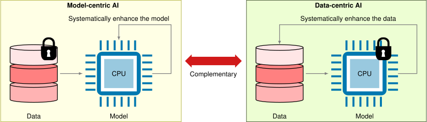](https://mlsysbook.ai/contents/core/benchmarking/e66c88ffc172d27f92b99b5454d93e446fa99392.svg "Figure 12: Development Paradigms: Model-centric AI prioritizes architectural innovation with fixed datasets, while data-centric AI systematically improves dataset quality (annotations, diversity, and bias) with consistent model architectures to achieve performance gains. Modern research indicates that strategic data enhancement often yields greater improvements than solely refining model complexity.")
Figure 12: **Development Paradigms**: Model-centric AI prioritizes architectural innovation with fixed datasets, while data-centric AI systematically improves dataset quality (annotations, diversity, and bias) with consistent model architectures to achieve performance gains. Modern research indicates that strategic data enhancement often yields greater improvements than solely refining model complexity.
Data quality’s primacy in AI development reflects a fundamental shift in understanding: superior datasets, not just sophisticated models, produce more reliable and robust AI systems. Initiatives like DataPerf and DataComp have emerged to systematically evaluate how dataset improvements affect model performance. For instance, DataComp ([Nishigaki 2024](https://mlsysbook.ai/contents/core/benchmarking/benchmarking.html#ref-gadre2024datacomp)
) demonstrated that models trained on a carefully curated 30% subset of data achieved better results than those trained on the complete dataset, challenging the assumption that more data automatically leads to better performance ([Northcutt, Athalye, and Mueller 2021](https://mlsysbook.ai/contents/core/benchmarking/benchmarking.html#ref-northcutt2021pervasive)
).
Nishigaki, Shinsuke. 2024. “Eigenphase Distributions of Unimodular Circular Ensembles.” _arXiv Preprint arXiv:2401.09045_ 36 (January). [http://arxiv.org/abs/2401.09045v2](http://arxiv.org/abs/2401.09045v2)
.
Northcutt, Curtis G., Anish Athalye, and Jonas Mueller. 2021. “Pervasive Label Errors in Test Sets Destabilize Machine Learning Benchmarks.” _arXiv Preprint arXiv:2103.14749_ 34 (March): 19075–90. [https://doi.org/10.48550/arxiv.2103.14749](https://doi.org/10.48550/arxiv.2103.14749)
.
A significant challenge in data benchmarking emerges from dataset saturation. When models achieve near-perfect accuracy on benchmarks like ImageNet, it becomes crucial to distinguish whether performance gains represent genuine advances in AI capability or merely optimization to existing test sets. [Figure 13](https://mlsysbook.ai/contents/core/benchmarking/benchmarking.html#fig-dataset-saturation)
illustrates this trend, showing AI systems surpassing human performance across various applications over the past decade.
[](https://mlsysbook.ai/contents/core/benchmarking/c4c5d7a34a48dee9b6266164bfe2fd31f7080e10.svg "Figure 13: Dataset Saturation: AI systems surpass human performance on benchmark datasets, indicating that continued gains may not reflect genuine improvements in intelligence but rather optimization to fixed evaluation sets. This trend underscores the need for dynamic, challenging datasets that accurately assess AI capabilities and drive meaningful progress beyond simple pattern recognition. Source: [@kiela2021dynabench].")
Figure 13: **Dataset Saturation**: AI systems surpass human performance on benchmark datasets, indicating that continued gains may not reflect genuine improvements in intelligence but rather optimization to fixed evaluation sets. This trend underscores the need for dynamic, challenging datasets that accurately assess AI capabilities and drive meaningful progress beyond simple pattern recognition. Source: ([Kiela et al. 2021](https://mlsysbook.ai/contents/core/benchmarking/benchmarking.html#ref-kiela2021dynabench)
).
This saturation phenomenon raises fundamental methodological questions ([Kiela et al. 2021](https://mlsysbook.ai/contents/core/benchmarking/benchmarking.html#ref-kiela2021dynabench)
). The MNIST dataset provides an illustrative example: certain test images, though nearly illegible to humans, were assigned specific labels during the dataset’s creation in 1994. When models correctly predict these labels, their apparent superhuman performance may actually reflect memorization of dataset artifacts rather than true digit recognition capabilities.
Kiela, Douwe, Max Bartolo, Yixin Nie, Divyansh Kaushik, Atticus Geiger, Zhengxuan Wu, Bertie Vidgen, et al. 2021. “Dynabench: Rethinking Benchmarking in NLP.” In _Proceedings of the 2021 Conference of the North American Chapter of the Association for Computational Linguistics: Human Language Technologies_, 9:418–34. Online: Association for Computational Linguistics. [https://doi.org/10.18653/v1/2021.naacl-main.324](https://doi.org/10.18653/v1/2021.naacl-main.324)
.
Beyer, Lucas, Olivier J. Hénaff, Alexander Kolesnikov, Xiaohua Zhai, and Aäron van den Oord. 2020. “Are We Done with ImageNet?” _arXiv Preprint arXiv:2006.07159_, June. [http://arxiv.org/abs/2006.07159v1](http://arxiv.org/abs/2006.07159v1)
.
These challenges extend beyond individual domains. The provocative question “Are we done with ImageNet?” ([Beyer et al. 2020](https://mlsysbook.ai/contents/core/benchmarking/benchmarking.html#ref-beyer2020we)
) highlights broader concerns about the limitations of static benchmarks. Models optimized for fixed datasets often struggle with distribution shifts, real-world changes that occur after training data collection. This limitation has driven the development of dynamic benchmarking approaches, such as Dynabench ([Kiela et al. 2021](https://mlsysbook.ai/contents/core/benchmarking/benchmarking.html#ref-kiela2021dynabench)
), which continuously evolves test data based on model performance to maintain benchmark relevance.
Current data benchmarking efforts encompass several critical dimensions. Label quality assessment remains a central focus, as explored in DataPerf’s debugging challenge. Initiatives like MSWC ([Mazumder et al. 2021](https://mlsysbook.ai/contents/core/benchmarking/benchmarking.html#ref-mazumder2021multilingual)
) for speech recognition address bias and representation in datasets. Out-of-distribution generalization receives particular attention through benchmarks like RxRx and WILDS ([Koh et al. 2021](https://mlsysbook.ai/contents/core/benchmarking/benchmarking.html#ref-koh2021wilds)
). These diverse efforts reflect a growing recognition that advancing AI capabilities requires not just better models and systems, but fundamentally better approaches to data quality assessment and benchmark design.
Mazumder, Mark, Sharad Chitlangia, Colby Banbury, Yiping Kang, Juan Manuel Ciro, Keith Achorn, Daniel Galvez, et al. 2021. “Multilingual Spoken Words Corpus.” In _Thirty-Fifth Conference on Neural Information Processing Systems Datasets and Benchmarks Track (Round 2)_.
Koh, Pang Wei, Shiori Sagawa, Henrik Marklund, Sang Michael Xie, Marvin Zhang, Akshay Balsubramani, Weihua Hu, et al. 2021. “WILDS: A Benchmark of in-the-Wild Distribution Shifts.” In _Proceedings of the 38th International Conference on Machine Learning, ICML 2021, 18-24 July 2021, Virtual Event_, edited by Marina Meila and Tong Zhang, 139:5637–64. Proceedings of Machine Learning Research. PMLR. [http://proceedings.mlr.press/v139/koh21a.html](http://proceedings.mlr.press/v139/koh21a.html)
.
### Holistic System-Model-Data Evaluation
AI benchmarking has traditionally evaluated systems, models, and data as separate entities. However, real-world AI performance emerges from the interplay between these three components. A fast system cannot compensate for a poorly trained model, and even the most powerful model is constrained by the quality of the data it learns from. This interdependence necessitates a holistic benchmarking approach that considers all three dimensions together.
As illustrated in [Figure 14](https://mlsysbook.ai/contents/core/benchmarking/benchmarking.html#fig-benchmarking-trifecta)
, the future of benchmarking lies in an integrated framework that jointly evaluates system efficiency, model performance, and data quality. This approach enables researchers to identify optimization opportunities that remain invisible when these components are analyzed in isolation. For example, co-designing efficient AI models with hardware-aware optimizations and carefully curated datasets can lead to superior performance while reducing computational costs.
[](https://mlsysbook.ai/contents/core/benchmarking/caab15d0f0e3f12e3793e85ecbbc14f74c6174e3.svg "Figure 14: AI System Interdependence: Highlights the critical interplay between infrastructure, models, and data in determining overall AI system performance, emphasizing that optimization requires a holistic approach rather than isolated improvements. this figure illustrates that gains in one component cannot fully compensate for limitations in others, necessitating co-design strategies for efficient and effective AI.")
Figure 14: **AI System Interdependence**: Highlights the critical interplay between infrastructure, models, and data in determining overall AI system performance, emphasizing that optimization requires a holistic approach rather than isolated improvements. this figure illustrates that gains in one component cannot fully compensate for limitations in others, necessitating co-design strategies for efficient and effective AI.
As AI continues to evolve, benchmarking methodologies must advance in tandem. Evaluating AI performance through the lens of systems, models, and data ensures that benchmarks drive improvements not just in accuracy, but also in efficiency, fairness, and robustness. This holistic perspective will be critical for developing AI that is not only powerful but also practical, scalable, and ethical.
**Self-Check: Question 1.11**
1. What is the primary goal of model benchmarking in AI systems?
1. To measure system efficiency
2. To determine hardware compatibility
3. To assess data quality
4. To evaluate algorithmic performance
2. True or False: Data benchmarking focuses solely on the size of the dataset used for training AI models.
3. Explain the challenge of benchmark optimization in Large Language Models (LLMs) and how it differs from traditional systems evaluation.
4. Order the following steps in a holistic AI benchmarking approach: (1) Evaluate model performance, (2) Assess data quality, (3) Measure system efficiency.
5. In a production system, how might you apply a data-centric approach to improve AI model performance?
[See Answers →](https://mlsysbook.ai/contents/core/benchmarking/benchmarking.html#quiz-answer-sec-benchmarking-ai-model-data-benchmarking-f058)
Production Environment Evaluation
---------------------------------
The benchmarking methodologies discussed thus far (from micro to end-to-end granularity, from training to inference evaluation) primarily address system performance under controlled conditions. However, the deployment strategies introduced in **[Chapter 13: ML Operations](https://mlsysbook.ai/contents/core/ops/ops.html#sec-ml-operations)
** reveal that production environments introduce distinctly different challenges requiring specialized evaluation approaches. Production machine learning systems must handle dynamic workloads, varying data quality, infrastructure failures, and concurrent user demands while maintaining consistent performance and reliability. This necessitates extending our benchmarking framework beyond single-point performance measurement to evaluate system behavior over time, under stress, and during failure scenarios.
Silent failure detection represents a critical production benchmarking dimension absent from research evaluation frameworks. Machine learning models can degrade silently without obvious error signals, producing plausible but incorrect outputs that escape traditional monitoring. Production benchmarking must establish baseline performance distributions and detect subtle accuracy degradation through statistical process control methods. A/B testing frameworks compare new model versions against stable baselines under identical traffic conditions, measuring not just average performance but performance variance and tail behavior.
Continuous data quality monitoring addresses the dynamic nature of production data streams that can introduce distribution shift, adversarial examples, or corrupted inputs. Production benchmarks must evaluate model robustness under realistic data quality variations including missing features, out-of-range values, and input format changes. Monitoring systems track feature distribution drift over time, measuring statistical distances between training and production data to predict when retraining becomes necessary. Data validation pipelines benchmark preprocessing robustness, ensuring models gracefully handle data quality issues without silent failures.
Load testing and capacity planning evaluate system performance under varying traffic patterns that reflect real user behavior. Production ML systems must handle request spikes, concurrent user sessions, and sustained high-throughput operation while maintaining latency requirements. Benchmarking protocols simulate realistic load patterns including diurnal traffic variations, flash traffic events, and organic growth scenarios. Capacity planning benchmarks measure how performance degrades as system utilization approaches limits, enabling proactive scaling decisions.
Operational resilience benchmarking evaluates system behavior during infrastructure failures, network partitions, and resource constraints. Production systems must maintain service availability during partial failures, gracefully degrade when resources become unavailable, and recover quickly from outages. Chaos engineering approaches systematically introduce failures to measure system resilience: killing inference servers, inducing network latency, and limiting computational resources to observe degradation patterns and recovery characteristics.
Multi-objective optimization in production requires benchmarking frameworks that balance accuracy, latency, cost, and resource utilization simultaneously. Production systems optimize for user experience metrics like conversion rates and engagement alongside traditional ML metrics. Cost efficiency benchmarks evaluate compute cost per prediction, storage costs for model artifacts, and operational overhead for system maintenance. Service level objectives (SLOs) define acceptable performance ranges across multiple dimensions, enabling systematic evaluation of production system health.
Continuous model validation implements automated benchmarking pipelines that evaluate model performance on held-out datasets and synthetic test cases over time. Shadow deployment techniques run new models alongside production systems, comparing outputs without affecting user experience. Champion-challenger frameworks systematically evaluate model improvements through controlled rollouts, measuring both performance improvements and potential negative impacts on downstream systems.
Production benchmarking therefore requires end-to-end evaluation frameworks that extend far beyond model accuracy to encompass system reliability, operational efficiency, and user experience optimization. This comprehensive approach ensures that ML systems deliver consistent value in dynamic production environments while maintaining the robustness necessary for mission-critical applications.
**Self-Check: Question 1.12**
1. Which of the following is a key challenge unique to production benchmarking in ML systems?
1. Evaluating algorithmic performance in isolation
2. Measuring training time efficiency
3. Optimizing model hyperparameters
4. Handling dynamic workloads and silent failures
2. True or False: Silent failure detection is adequately addressed by traditional research evaluation frameworks.
3. Why is continuous data quality monitoring essential in production ML systems?
4. Order the following steps in a production benchmarking process: (1) Evaluate system behavior during failures, (2) Monitor data quality, (3) Conduct load testing.
5. In a production system, what trade-offs would you consider when implementing chaos engineering for resilience benchmarking?
[See Answers →](https://mlsysbook.ai/contents/core/benchmarking/benchmarking.html#quiz-answer-sec-benchmarking-ai-production-environment-evaluation-7512)
Fallacies and Pitfalls
----------------------
The benchmarking methodologies and frameworks established throughout this chapter (from our three-dimensional evaluation framework to the specific metrics for training and inference) provide powerful tools for systematic evaluation. However, their effectiveness depends critically on avoiding common misconceptions and methodological errors that can undermine benchmark validity. The standardized nature of benchmarks, while enabling fair comparison, often creates false confidence about their universal applicability.
**Fallacy:** _Benchmark performance directly translates to real-world application performance._
This misconception leads teams to select models and systems based solely on benchmark rankings without considering deployment context differences. Benchmarks typically use curated datasets, standardized evaluation protocols, and optimal configurations that rarely match real-world conditions. Production systems face data quality issues, distribution shifts, latency constraints, and resource limitations not captured in benchmark scenarios. A model that achieves state-of-the-art benchmark performance might fail catastrophically when deployed due to these environmental differences. Effective system selection requires augmenting benchmark results with deployment-specific evaluation rather than relying solely on standardized metrics.
**Pitfall:** _Optimizing exclusively for benchmark metrics without considering broader system requirements._
Many practitioners focus intensively on improving benchmark scores without understanding how these optimizations affect overall system behavior. Techniques that boost specific metrics might degrade other important characteristics like robustness, calibration, fairness, or energy efficiency. Overfitting to benchmark evaluation protocols can create models that perform well on specific test conditions but fail to generalize to varied real-world scenarios. This narrow optimization approach, a manifestation of Goodhart’s Law[53](https://mlsysbook.ai/contents/core/benchmarking/benchmarking.html#fn53)
discussed in [Section 1.10.4.1](https://mlsysbook.ai/contents/core/benchmarking/benchmarking.html#sec-benchmarking-ai-benchmark-engineering-99d3)
, often produces systems that excel in controlled environments but struggle with the complexity and unpredictability of practical deployments.
53 **Goodhart’s Law**: Originally articulated by British economist Charles Goodhart in 1975, this principle states: “When a measure becomes a target, it ceases to be a good measure.” In ML systems benchmarking, this captures the fundamental tension between using benchmarks as indicators of system quality and the tendency for practitioners to optimize specifically for benchmark scores rather than underlying performance characteristics. As benchmarks become targets for optimization, they progressively lose their value as meaningful proxies for real-world system effectiveness.
**Fallacy:** _Single-metric evaluation provides sufficient insight into system performance._
This belief assumes that one primary metric captures all relevant aspects of system performance. Modern AI systems require evaluation across multiple dimensions including accuracy, latency, throughput, energy consumption, fairness, and robustness. Optimizing for accuracy alone might create systems with unacceptable inference delays, while focusing on throughput might compromise result quality. Different stakeholders prioritize different metrics, and deployment contexts create varying constraints that single metrics cannot capture. Comprehensive evaluation requires multidimensional assessment frameworks that reveal trade-offs across all relevant performance aspects.
**Pitfall:** _Using outdated benchmarks that no longer reflect current challenges and requirements._
Teams often continue using established benchmarks long after they cease to represent meaningful challenges or current deployment realities. As model capabilities advance, benchmarks can become saturated, providing little discriminatory power between approaches. Similarly, changing application requirements, new deployment contexts, and evolving fairness standards can make existing benchmarks irrelevant or misleading. Benchmark datasets may also develop hidden biases or quality issues over time as they age. Effective benchmarking requires regular assessment of whether evaluation frameworks still provide meaningful insights for current challenges and deployment scenarios.
**Pitfall:** _Applying research-oriented benchmarks to evaluate production system performance without accounting for operational constraints._
Many teams use academic benchmarks designed for research comparisons to evaluate production systems, overlooking fundamental differences between research and operational environments. Research benchmarks typically assume unlimited computational resources, optimal data quality, and idealized deployment conditions that rarely exist in production settings. Production systems must handle concurrent user loads, varying input quality, network latency, memory constraints, and system failures that significantly impact performance compared to controlled benchmark conditions. Additionally, production systems require optimization for multiple objectives simultaneously including cost efficiency, availability, and user experience that single-metric research benchmarks cannot capture. Effective production evaluation requires augmenting research benchmarks with operational metrics like sustained throughput under load, recovery time from failures, resource utilization efficiency, and end-to-end latency including data preprocessing and postprocessing overhead.
**Self-Check: Question 1.13**
1. Which of the following is a common fallacy regarding benchmark performance in ML systems?
1. Benchmark performance directly translates to real-world application performance.
2. Benchmarks should be used as a sole metric for model selection.
3. Benchmarks are irrelevant for production systems.
4. Benchmarks always reflect the latest challenges in ML.
2. Why is optimizing exclusively for benchmark metrics without considering broader system requirements a pitfall in ML system development?
3. True or False: Using outdated benchmarks can lead to misleading insights about current ML system performance.
4. Order the following steps for evaluating production system performance using benchmarks: (1) Assess operational constraints, (2) Analyze benchmark results, (3) Augment with deployment-specific metrics.
5. In a production system, how might you address the challenge of benchmarks not aligning with real-world deployment goals?
[See Answers →](https://mlsysbook.ai/contents/core/benchmarking/benchmarking.html#quiz-answer-sec-benchmarking-ai-fallacies-pitfalls-620e)
Summary
-------
This chapter established benchmarking as the critical measurement discipline that validates the performance claims and optimization strategies introduced throughout Parts II and III. By developing a comprehensive three-dimensional framework evaluating algorithms, systems, and data simultaneously, we demonstrated how systematic measurement transforms the theoretical advances in efficient AI design (**[Chapter 9: Efficient AI](https://mlsysbook.ai/contents/core/efficient_ai/efficient_ai.html#sec-efficient-ai)
**), model optimization (**[Chapter 10: Model Optimizations](https://mlsysbook.ai/contents/core/optimizations/optimizations.html#sec-model-optimizations)
**), and hardware acceleration (**[Chapter 11: AI Acceleration](https://mlsysbook.ai/contents/core/hw_acceleration/hw_acceleration.html#sec-ai-acceleration)
**) into quantifiable engineering improvements. The progression from historical computing benchmarks through specialized ML evaluation methodologies revealed why modern AI systems require multifaceted assessment approaches that capture the complexity of real-world deployment.
The technical sophistication of modern benchmarking frameworks reveals how measurement methodology directly influences innovation direction and resource allocation decisions across the entire AI ecosystem. System benchmarks like MLPerf drive hardware optimization and infrastructure development by establishing standardized workloads and metrics that enable fair comparison across diverse architectures. Model benchmarks push algorithmic innovation by defining challenging tasks and evaluation protocols that reveal limitations and guide research priorities. Data benchmarks expose critical issues around representation, bias, and quality that directly impact model fairness and generalization capabilities. The integration of these benchmarking dimensions creates a comprehensive evaluation framework that captures the complexity of real-world AI deployment challenges.
Key Takeaways
* Effective benchmarking requires multidimensional evaluation across systems, models, and data to capture real-world deployment challenges
* Standardized benchmarks like MLPerf drive hardware innovation and enable fair comparison across diverse architectures and implementations
* Benchmark design choices fundamentally shape research priorities and resource allocation across the entire AI ecosystem
* Future benchmarking must evolve to address emerging challenges around AI safety, fairness, and environmental impact
The benchmarking foundations established here provide the measurement infrastructure necessary for the operational deployment strategies explored in Part IV: Robust Deployment. The transition from performance measurement to production deployment requires extending benchmark validation beyond laboratory conditions. While this chapter focused on systematic evaluation under controlled conditions, Part IV addresses the additional complexities of dynamic workloads, evolving data distributions, and operational constraints that characterize real-world ML system deployment. In **[Chapter 13: ML Operations](https://mlsysbook.ai/contents/core/ops/ops.html#sec-ml-operations)
**, we extend these benchmarking principles to production environments, where continuous monitoring detects silent failures, tracks model performance degradation, and validates system behavior under dynamic workloads that offline benchmarks cannot capture. The A/B testing frameworks and champion-challenger methodologies introduced in production monitoring build directly upon the comparative evaluation principles established through training and inference benchmarking.
The privacy and security challenges in **[Chapter 15: Security & Privacy](https://mlsysbook.ai/contents/core/privacy_security/privacy_security.html#sec-security-privacy)
** similarly require specialized benchmarking methodologies that evaluate dimensions beyond pure performance. Adversarial robustness benchmarks measure model resilience against intentional attacks, while privacy-preserving computation frameworks require benchmarking trade-offs between utility and privacy guarantees. The robustness requirements in **[Chapter 16: Robust AI](https://mlsysbook.ai/contents/core/robust_ai/robust_ai.html#sec-robust-ai)
** demand evaluation protocols that assess model behavior under distribution shift, data corruption, and edge cases that traditional benchmarks overlook.
As AI systems become increasingly influential in critical applications, the benchmarking frameworks developed today determine whether we can effectively measure and optimize for societal impacts extending far beyond traditional performance metrics. The responsible AI principles in **[Chapter 17: Responsible AI](https://mlsysbook.ai/contents/core/responsible_ai/responsible_ai.html#sec-responsible-ai)
** and sustainability considerations in **[Chapter 18: Sustainable AI](https://mlsysbook.ai/contents/core/sustainable_ai/sustainable_ai.html#sec-sustainable-ai)
** establish new evaluation dimensions that must be integrated alongside efficiency and accuracy in comprehensive system assessment.
**Self-Check: Question 1.14**
1. What is the primary role of benchmarking in AI systems as discussed in this section?
1. To validate performance claims and optimization strategies.
2. To provide a theoretical framework for AI model development.
3. To replace traditional computing benchmarks entirely.
4. To focus solely on hardware performance improvements.
2. Explain how benchmarking influences innovation direction and resource allocation in AI systems.
3. True or False: Benchmarking frameworks like MLPerf are primarily concerned with algorithmic innovation.
4. In a production system, how might you apply benchmarking principles to address model fairness and generalization capabilities?
[See Answers →](https://mlsysbook.ai/contents/core/benchmarking/benchmarking.html#quiz-answer-sec-benchmarking-ai-summary-52a3)
Self-Check Answers
------------------
**Self-Check: Answer 1.1**
1. **What is the primary purpose of benchmarking in machine learning systems?**
1. To optimize algorithmic theory
2. To focus solely on computational efficiency
3. To establish empirical baselines for performance evaluation
4. To replace traditional computational benchmarking
_Answer_: The correct answer is C. To establish empirical baselines for performance evaluation. This is correct because benchmarking provides systematic evaluation frameworks to compare and validate ML system performance across different contexts. Options A, B, and D do not capture the comprehensive role of benchmarking as described.
_Learning Objective_: Understand the role of benchmarking in evaluating ML system performance.
2. **True or False: Traditional deterministic benchmarks are sufficient for evaluating the performance of machine learning systems.**
_Answer_: False. This is false because ML systems have probabilistic elements and complex dependencies that traditional deterministic benchmarks cannot adequately characterize.
_Learning Objective_: Recognize the limitations of traditional benchmarks in the context of ML systems.
3. **Why is it challenging to evaluate machine learning systems using conventional performance metrics?**
_Answer_: Evaluating ML systems is challenging due to their probabilistic nature, which introduces performance variability. Additionally, ML systems have complex dependencies on data, model architectures, and computational resources, requiring multi-dimensional evaluation approaches. For example, a model’s predictive accuracy might trade off against computational efficiency. This is important because it necessitates specialized benchmarking methodologies.
_Learning Objective_: Analyze the challenges involved in evaluating ML systems using conventional metrics.
4. **Which of the following is NOT a dimension that contemporary ML systems must be evaluated on?**
1. Predictive accuracy
2. Convergence properties
3. Energy consumption
4. Aesthetic design
_Answer_: The correct answer is D. Aesthetic design. This is correct because the evaluation dimensions listed in the section focus on performance metrics relevant to ML systems, such as predictive accuracy, convergence, and energy consumption, rather than design aesthetics.
_Learning Objective_: Identify the key dimensions for evaluating ML systems.
[← Back to Questions](https://mlsysbook.ai/contents/core/benchmarking/benchmarking.html#quiz-question-sec-benchmarking-ai-machine-learning-benchmarking-framework-3968)
**Self-Check: Answer 1.2**
1. **Which of the following represents a key shift in the evolution of performance benchmarks from early computing to modern ML systems?**
1. Focus on isolated operations rather than integrated systems
2. Evaluation based on single metrics instead of multi-objective evaluation
3. Use of synthetic tests over representative workloads
4. Optimization for narrow tests rather than practical performance
_Answer_: The correct answer is B. Evaluation based on single metrics instead of multi-objective evaluation. This shift reflects the need to capture multiple dimensions of performance, such as accuracy, latency, and energy efficiency, in modern ML systems.
_Learning Objective_: Understand the historical shifts in benchmarking approaches and their significance for ML systems.
2. **True or False: The shift from isolated component evaluation to integrated system evaluation was driven by the realization that component optimization alone does not predict overall system performance.**
_Answer_: True. This is true because distributed computing revealed that optimizing individual components does not necessarily lead to improved system performance, highlighting the importance of evaluating integrated systems.
_Learning Objective_: Recognize the importance of evaluating ML systems as integrated entities rather than isolated components.
3. **How does the inclusion of real models like ResNet-50 and BERT in MLPerf benchmarks ensure more accurate evaluation of ML systems?**
_Answer_: Including real models like ResNet-50 and BERT in MLPerf benchmarks ensures that the evaluation reflects the complexity and challenges of actual deployment scenarios. This approach prevents gaming of benchmarks through narrow optimizations and provides a more comprehensive assessment of system performance.
_Learning Objective_: Explain the role of representative workloads in providing accurate ML system evaluations.
4. **What is a primary challenge in energy benchmarking for AI systems?**
1. Accounting for diverse workload patterns and system configurations
2. Measuring only hardware energy consumption
3. Focusing solely on algorithmic energy optimization
4. Ignoring the impact of neural network pruning
_Answer_: The correct answer is A. Accounting for diverse workload patterns and system configurations. This challenge arises because energy benchmarking must consider the variability in how AI systems are deployed and used across different environments.
_Learning Objective_: Identify challenges in energy benchmarking for AI systems and the importance of comprehensive evaluation.
[← Back to Questions](https://mlsysbook.ai/contents/core/benchmarking/benchmarking.html#quiz-question-sec-benchmarking-ai-historical-context-1c54)
**Self-Check: Answer 1.3**
1. **What is a key difference between traditional benchmarks and AI benchmarks?**
1. AI benchmarks focus solely on computational speed.
2. Traditional benchmarks include data quality as a primary factor.
3. AI benchmarks incorporate variability and accuracy as evaluation dimensions.
4. Traditional benchmarks are more complex than AI benchmarks.
_Answer_: The correct answer is C. AI benchmarks incorporate variability and accuracy as evaluation dimensions. This is correct because AI systems exhibit inherent variability due to their probabilistic nature, unlike traditional deterministic benchmarks.
_Learning Objective_: Understand the unique characteristics of AI benchmarks compared to traditional benchmarks.
2. **Explain why energy efficiency is considered a cross-cutting concern in the three-dimensional evaluation framework for ML benchmarks.**
_Answer_: Energy efficiency impacts all three dimensions of the evaluation framework: it influences algorithmic choices, affects hardware performance, and is impacted by dataset characteristics. For example, algorithmic complexity affects power requirements, while hardware capabilities determine energy-performance trade-offs. This is important because it ensures that ML systems are not only effective but also sustainable.
_Learning Objective_: Analyze the role of energy efficiency in the comprehensive evaluation of ML systems.
3. **True or False: The inherent variability in ML systems makes it unnecessary to run multiple experimental trials when benchmarking.**
_Answer_: False. This is false because the inherent variability in ML systems requires multiple experimental trials to distinguish genuine performance improvements from measurement noise. Statistical measures like standard deviations or confidence intervals are necessary for accurate assessment.
_Learning Objective_: Evaluate the necessity of rigorous statistical methodologies in ML benchmarking.
4. **Order the following steps for effective ML benchmarking: (1) Evaluate algorithmic performance, (2) Measure system performance, (3) Assess data quality.**
_Answer_: The correct order is: (1) Evaluate algorithmic performance, (3) Assess data quality, (2) Measure system performance. This order reflects the three-dimensional framework where algorithmic performance is isolated first, data quality is assessed for its impact on model behavior, and finally, system performance is measured to understand the hardware’s role.
_Learning Objective_: Understand the sequence and interrelation of different benchmarking dimensions in ML systems.
[← Back to Questions](https://mlsysbook.ai/contents/core/benchmarking/benchmarking.html#quiz-question-sec-benchmarking-ai-machine-learning-benchmarks-6b88)
**Self-Check: Answer 1.4**
1. **Which of the following best describes the purpose of micro-benchmarks in ML systems?**
1. To evaluate the entire ML pipeline for production readiness.
2. To assess individual operations like tensor computations for optimization.
3. To compare different ML models on standard datasets.
4. To evaluate the performance of storage and network systems.
_Answer_: The correct answer is B. To assess individual operations like tensor computations for optimization. Micro-benchmarks focus on specific components within ML systems, providing detailed insights into computational demands.
_Learning Objective_: Understand the role of micro-benchmarks in optimizing specific ML system components.
2. **Discuss the trade-offs between micro-benchmarks and end-to-end benchmarks in ML systems.**
_Answer_: Micro-benchmarks offer high diagnostic precision for isolated components, allowing detailed optimization. However, they lack real-world representativeness. End-to-end benchmarks provide a comprehensive view of system performance, capturing complex interactions but offering less precision at the component level. This is important because combining both allows for balanced system evaluation.
_Learning Objective_: Analyze the trade-offs between different benchmarking approaches in ML systems.
3. **Order the following benchmarking levels from most isolated to most comprehensive: (1) Macro-benchmarks, (2) Micro-benchmarks, (3) End-to-end benchmarks.**
_Answer_: The correct order is: (2) Micro-benchmarks, (1) Macro-benchmarks, (3) End-to-end benchmarks. Micro-benchmarks focus on individual operations, macro-benchmarks assess complete models, and end-to-end benchmarks evaluate the entire system pipeline.
_Learning Objective_: Sequence the benchmarking levels based on their scope and comprehensiveness.
4. **What is a primary challenge of using end-to-end benchmarks in ML systems?**
1. They provide too much detail on individual operations.
2. They often miss system-level bottlenecks.
3. They focus only on model accuracy, ignoring infrastructure.
4. They are complex to standardize and often proprietary.
_Answer_: The correct answer is D. They are complex to standardize and often proprietary. End-to-end benchmarks assess full system performance but face challenges in standardization due to their comprehensive nature.
_Learning Objective_: Identify challenges associated with end-to-end benchmarking in ML systems.
[← Back to Questions](https://mlsysbook.ai/contents/core/benchmarking/benchmarking.html#quiz-question-sec-benchmarking-ai-benchmarking-granularity-771c)
**Self-Check: Answer 1.5**
1. **Which of the following components is NOT typically part of a benchmark implementation in machine learning systems?**
1. Task definition
2. Dataset selection
3. Evaluation metrics
4. User interface design
_Answer_: The correct answer is D. User interface design. This is correct because benchmark implementations focus on task definition, dataset selection, model selection, and evaluation metrics. User interface design is not a standard component in benchmarking.
_Learning Objective_: Identify the key components involved in implementing a benchmark for ML systems.
2. **True or False: Micro-benchmarks focus on evaluating the entire system performance rather than individual components.**
_Answer_: False. Micro-benchmarks focus on evaluating individual components, such as tensor operations, to isolate specific computational patterns.
_Learning Objective_: Understand the purpose and focus of micro-benchmarks within the benchmarking framework.
3. **Explain how the selection of a dataset influences the effectiveness of a benchmark in evaluating machine learning models.**
_Answer_: The selection of a dataset is crucial as it ensures models are tested under identical conditions, allowing direct comparisons. Effective datasets must accurately represent real-world challenges and maintain complexity to differentiate model performance. For example, using ToyADMOS for anomaly detection ensures models are evaluated on representative audio data, reflecting real deployment conditions.
_Learning Objective_: Analyze the impact of dataset selection on benchmark effectiveness and model evaluation.
4. **Order the following components in the benchmark workflow: (1) Model selection, (2) Problem definition, (3) Evaluation metrics, (4) Dataset selection.**
_Answer_: The correct order is: (2) Problem definition, (4) Dataset selection, (1) Model selection, (3) Evaluation metrics. This order reflects the systematic progression from defining the problem, selecting appropriate datasets, choosing models, and finally determining the metrics for evaluation.
_Learning Objective_: Understand the sequential workflow involved in setting up a benchmark for ML systems.
5. **In a production system, what trade-offs might you consider when selecting evaluation metrics for a benchmark?**
_Answer_: In a production system, trade-offs include balancing accuracy with computational efficiency, such as processing speed and energy consumption. For instance, a high accuracy model may require more resources, impacting real-time performance. Selecting metrics like AUC for accuracy and milliseconds per inference for speed ensures the model meets both technical and operational requirements.
_Learning Objective_: Evaluate trade-offs in selecting evaluation metrics for benchmarks in real-world ML systems.
[← Back to Questions](https://mlsysbook.ai/contents/core/benchmarking/benchmarking.html#quiz-question-sec-benchmarking-ai-benchmark-components-1bf1)
**Self-Check: Answer 1.6**
1. **What is a key difference between the training and inference phases in ML systems regarding computational processes?**
1. Training involves only forward passes with fixed model parameters.
2. Inference requires bidirectional computation with forward and backward passes.
3. Training requires bidirectional computation with forward and backward passes.
4. Inference involves iterative optimization over large datasets.
_Answer_: The correct answer is C. Training requires bidirectional computation with forward and backward passes. This is correct because training involves optimizing model parameters through gradient descent, which requires both forward and backward passes. Inference, on the other hand, only requires forward passes with fixed parameters. Options A and D incorrectly describe the phases, and B is incorrect because inference does not involve backward passes.
_Learning Objective_: Understand the computational differences between training and inference phases.
2. **Explain why training can afford to sacrifice latency for throughput, while inference prioritizes latency consistency.**
_Answer_: Training can afford to sacrifice latency for throughput because it focuses on processing large batches of data to optimize model parameters efficiently, often over extended periods. In contrast, inference prioritizes latency consistency to ensure quick response times for individual queries, which is crucial for real-time applications. For example, training might process 10,000 samples per second, while inference needs to respond in milliseconds. This is important because it affects how resources are allocated and managed in ML systems.
_Learning Objective_: Analyze the trade-offs between latency and throughput in training and inference.
3. **Which of the following optimization strategies is unique to the inference phase in ML systems?**
1. Post-training quantization
2. Mixed-precision training
3. Gradient compression
4. Progressive pruning
_Answer_: The correct answer is A. Post-training quantization. This is correct because post-training quantization reduces the model size and speeds up inference by using lower precision data types, which is specifically beneficial for inference. Gradient compression and mixed-precision training are used during training to optimize memory and computation, while progressive pruning is also a training optimization technique.
_Learning Objective_: Identify specific optimization strategies used in the inference phase.
4. **During the training phase, mixed-precision training can reduce memory usage by \_\_\_\_ while maintaining convergence.**
_Answer_: 50%. Mixed-precision training uses lower precision data types to reduce memory usage during training, allowing for larger batch sizes and faster training without significantly impacting model accuracy.
_Learning Objective_: Recall the impact of mixed-precision training on memory usage.
5. **In a production system, what considerations would you make when deciding between optimizing for training throughput versus inference latency?**
_Answer_: In a production system, optimizing for training throughput is crucial when the focus is on rapid model development and iteration, allowing for faster convergence and model updates. However, optimizing for inference latency is essential when the system needs to handle real-time requests efficiently, ensuring user satisfaction with quick response times. The decision depends on the system’s operational goals and the trade-offs between resource allocation and performance requirements. This is important because it directly impacts the user experience and operational costs.
_Learning Objective_: Evaluate the practical trade-offs between training throughput and inference latency in real-world systems.
[← Back to Questions](https://mlsysbook.ai/contents/core/benchmarking/benchmarking.html#quiz-question-sec-benchmarking-ai-training-vs-inference-evaluation-cee8)
**Self-Check: Answer 1.7**
1. **Which of the following is a primary focus of ML training benchmarks?**
1. Evaluating inference latency
2. Measuring model accuracy on test data
3. Assessing training time-to-accuracy
4. Analyzing data preprocessing speed
_Answer_: The correct answer is C. Assessing training time-to-accuracy. This is correct because training benchmarks specifically focus on evaluating how quickly a model reaches a target accuracy during the training phase. Options A and B relate to inference and testing, while D is a component but not the primary focus.
_Learning Objective_: Understand the primary focus of ML training benchmarks.
2. **Explain why scalability is a critical consideration in training benchmarks for large-scale models.**
_Answer_: Scalability is critical because it determines how well a training system can handle increased computational resources, such as additional GPUs or TPUs, to reduce training time. Efficient scalability ensures that adding more resources leads to meaningful performance improvements. For example, doubling the number of GPUs should ideally halve the training time. This is important because large-scale models like GPT-3 require distributed computing to manage their computational demands.
_Learning Objective_: Analyze the importance of scalability in training benchmarks for large-scale models.
3. **Training benchmarks help identify bottlenecks in \_\_\_\_, gradient computation, and parameter synchronization.**
_Answer_: data loading. Training benchmarks focus on identifying inefficiencies in data loading, which can significantly impact the overall training performance.
_Learning Objective_: Recall key areas where training benchmarks identify bottlenecks.
4. **True or False: Training benchmarks only focus on hardware performance and ignore software optimizations.**
_Answer_: False. Training benchmarks evaluate both hardware performance and software optimizations, such as mixed-precision training and data loading efficiency, to ensure comprehensive system evaluation.
_Learning Objective_: Understand the scope of training benchmarks in evaluating both hardware and software performance.
5. **In a production system, what trade-offs would you consider when selecting hardware for training large-scale models?**
_Answer_: When selecting hardware, consider trade-offs between cost, performance, and energy efficiency. High-performance GPUs or TPUs may offer faster training times but at a higher cost and energy consumption. Balancing these factors is crucial for cost-effective and sustainable training. For example, while TPUs might offer superior performance for tensor operations, their cost and energy usage must align with the project’s budget and sustainability goals.
_Learning Objective_: Evaluate trade-offs in hardware selection for training large-scale models in production systems.
[← Back to Questions](https://mlsysbook.ai/contents/core/benchmarking/benchmarking.html#quiz-question-sec-benchmarking-ai-training-benchmarks-7533)
**Self-Check: Answer 1.8**
1. **Which of the following metrics is most critical for evaluating real-time inference performance?**
1. Tail Latency
2. Mean Latency
3. Throughput
4. Memory Footprint
_Answer_: The correct answer is A. Tail Latency. Tail latency is crucial for real-time applications as it measures worst-case delays, ensuring reliability under peak loads. Throughput and memory footprint are important but do not capture real-time performance issues.
_Learning Objective_: Understand the importance of tail latency in real-time inference applications.
2. **Explain why precision optimization techniques are important in inference benchmarks and what trade-offs they might involve.**
_Answer_: Precision optimization techniques, such as using FP16 or INT8, are important because they reduce computational load and memory usage, leading to faster inference and lower power consumption. However, these techniques may introduce accuracy degradation, requiring careful calibration to balance speed and precision. For example, INT8 can achieve 4x speedup but may reduce model accuracy if not properly calibrated. This is important because it allows for efficient deployment on resource-constrained devices.
_Learning Objective_: Analyze the trade-offs involved in precision optimization for inference performance.
3. **True or False: Inference benchmarks primarily focus on the training phase of machine learning models.**
_Answer_: False. Inference benchmarks focus on the deployment phase, evaluating how efficiently models make predictions in real-world environments. This includes assessing latency, throughput, and resource utilization during model serving.
_Learning Objective_: Differentiate between the focus of inference and training benchmarks.
4. **Order the following factors in terms of their impact on inference efficiency: (1) Model architecture, (2) Hardware configuration, (3) Precision optimization.**
_Answer_: The correct order is: (1) Model architecture, (3) Precision optimization, (2) Hardware configuration. Model architecture determines the computational complexity, precision optimization affects speed and accuracy, and hardware configuration influences how efficiently resources are utilized.
_Learning Objective_: Evaluate the relative impact of different factors on inference efficiency.
5. **What is a key consideration when deploying inference systems on edge devices?**
1. Maximizing throughput
2. Maximizing model size
3. Minimizing power consumption
4. Minimizing training time
_Answer_: The correct answer is C. Minimizing power consumption. Edge devices have limited power resources, so minimizing power consumption is crucial to ensure sustained operation and efficiency. Throughput and model size are less critical in this context.
_Learning Objective_: Understand the constraints and priorities for deploying inference systems on edge devices.
[← Back to Questions](https://mlsysbook.ai/contents/core/benchmarking/benchmarking.html#quiz-question-sec-benchmarking-ai-inference-benchmarks-433b)
**Self-Check: Answer 1.9**
1. **Which of the following is a fundamental challenge in creating standardized energy efficiency benchmarks for ML systems?**
1. Absence of performance benchmarks
2. Lack of available hardware for testing
3. Inconsistent software development practices
4. Variability in power demands across different ML deployment environments
_Answer_: The correct answer is D. Variability in power demands across different ML deployment environments. This is correct because the power demands range from microwatts in TinyML devices to kilowatts in data centers, making standardization challenging. Other options do not directly address the core challenge of power variability.
_Learning Objective_: Understand the challenges in standardizing energy efficiency benchmarks due to diverse power requirements.
2. **True or False: System-level power measurement provides a more comprehensive view of energy consumption than measuring individual components.**
_Answer_: True. This is true because system-level measurement accounts for interactions between compute units, memory systems, and infrastructure, offering a holistic view of energy consumption.
_Learning Objective_: Recognize the advantages of system-level power measurement over component-level metrics.
3. **Explain why dynamic voltage and frequency scaling (DVFS) is important in optimizing energy efficiency in ML systems.**
_Answer_: DVFS is important because it adjusts processor voltage and frequency based on workload demands, reducing power consumption during periods of low computational intensity. For example, it can lower cooling requirements and overall power draw in data centers. This is important because it helps manage energy efficiency dynamically, adapting to varying workloads.
_Learning Objective_: Analyze the role of DVFS in optimizing energy efficiency in ML systems.
4. **The Power Usage Effectiveness (PUE) metric is used to measure the efficiency of a data center’s \_\_\_\_\_\_.**
_Answer_: cooling systems. This metric evaluates the ratio of total facility energy consumption to the energy used by computing equipment.
_Learning Objective_: Recall the purpose of the PUE metric in assessing data center efficiency.
5. **In a production system, what trade-offs would you consider when optimizing for energy efficiency versus computational performance?**
_Answer_: When optimizing for energy efficiency versus computational performance, one must consider the trade-off between achieving high performance and minimizing energy usage. For example, increasing processor frequency can enhance performance but also significantly raise power consumption. This is important because balancing these factors is crucial for sustainable ML system deployment, especially in energy-constrained environments.
_Learning Objective_: Evaluate trade-offs between energy efficiency and computational performance in ML systems.
[← Back to Questions](https://mlsysbook.ai/contents/core/benchmarking/benchmarking.html#quiz-question-sec-benchmarking-ai-power-measurement-techniques-ed95)
**Self-Check: Answer 1.10**
1. **Which of the following is a major limitation of current benchmarking practices in machine learning systems?**
1. Complete problem coverage
2. Perfect reproducibility
3. Hardware independence
4. Statistical insignificance
_Answer_: The correct answer is D. Statistical insignificance. This is correct because benchmarking often involves too few data samples, leading to unreliable results. Options A, B, and C are incorrect as they do not represent major limitations discussed in the section.
_Learning Objective_: Understand the key limitations of current benchmarking practices.
2. **How can the ‘hardware lottery’ affect the perceived performance of machine learning models in benchmarking?**
_Answer_: The hardware lottery affects perceived performance by favoring models that align well with current hardware capabilities, such as GPUs, potentially overlooking architectures that might perform better on different hardware. This is important because it can bias research and development towards hardware-compatible models rather than intrinsically superior ones.
_Learning Objective_: Analyze the impact of hardware compatibility on benchmarking outcomes.
3. **True or False: Reproducibility in benchmarking can be fully achieved by standardizing test environments.**
_Answer_: False. This is false because while standardizing test environments helps, reproducibility is also affected by factors like hardware configurations and software dependencies, which can still introduce variability.
_Learning Objective_: Evaluate the challenges in achieving reproducibility in benchmarking.
4. **What strategy can help mitigate the issue of benchmarks not aligning with real-world deployment goals?**
1. Conducting application-specific testing
2. Focusing solely on accuracy metrics
3. Ignoring environmental conditions
4. Standardizing hardware platforms
_Answer_: The correct answer is A. Conducting application-specific testing. This is correct because it ensures that models are evaluated in environments that mimic real-world conditions, addressing the misalignment issue. Options B, C, and D are incorrect as they do not directly address the alignment with real-world goals.
_Learning Objective_: Identify strategies to improve the alignment of benchmarks with real-world objectives.
5. **In a production system, how might you address the challenge of environmental conditions affecting benchmark results?**
_Answer_: In a production system, controlling environmental conditions such as temperature and background processes is crucial. For example, conducting experiments in temperature-controlled environments and documenting all operational conditions can help ensure consistent and reliable benchmark results. This is important because it minimizes external variability that could skew performance assessments.
_Learning Objective_: Apply knowledge of environmental conditions to improve benchmarking reliability in production systems.
[← Back to Questions](https://mlsysbook.ai/contents/core/benchmarking/benchmarking.html#quiz-question-sec-benchmarking-ai-benchmarking-limitations-best-practices-9b2a)
**Self-Check: Answer 1.11**
1. **What is the primary goal of model benchmarking in AI systems?**
1. To measure system efficiency
2. To determine hardware compatibility
3. To assess data quality
4. To evaluate algorithmic performance
_Answer_: The correct answer is D. To evaluate algorithmic performance. Model benchmarking focuses on assessing how well different machine learning algorithms perform on specific tasks, beyond just system efficiency.
_Learning Objective_: Understand the purpose of model benchmarking in AI systems.
2. **True or False: Data benchmarking focuses solely on the size of the dataset used for training AI models.**
_Answer_: False. Data benchmarking emphasizes the quality, diversity, and bias of datasets, not just their size, to ensure AI models learn effectively.
_Learning Objective_: Recognize the key aspects of data benchmarking beyond dataset size.
3. **Explain the challenge of benchmark optimization in Large Language Models (LLMs) and how it differs from traditional systems evaluation.**
_Answer_: In LLMs, benchmark optimization occurs when models are exposed to benchmark datasets during training, leading to memorization rather than genuine capability. This contrasts with traditional systems evaluation, where optimization is achieved through explicit code changes. For example, an LLM might perform well on a benchmark because it has seen similar data during training, not due to true understanding. This is important because it questions the validity of current evaluation methodologies.
_Learning Objective_: Analyze the unique challenges of benchmark optimization in LLMs compared to traditional systems.
4. **Order the following steps in a holistic AI benchmarking approach: (1) Evaluate model performance, (2) Assess data quality, (3) Measure system efficiency.**
_Answer_: The correct order is: (3) Measure system efficiency, (1) Evaluate model performance, (2) Assess data quality. This order reflects the integrated approach to benchmarking, where system, model, and data evaluations are interdependent and collectively determine AI performance.
_Learning Objective_: Understand the integrated approach to AI benchmarking, considering system, model, and data evaluations.
5. **In a production system, how might you apply a data-centric approach to improve AI model performance?**
_Answer_: A data-centric approach involves systematically improving dataset quality through better annotations, increased diversity, and bias reduction. For example, enhancing the dataset used for training a facial recognition model by ensuring it includes diverse skin tones can improve model fairness and accuracy. This is important because superior datasets can lead to more reliable and robust AI systems, often yielding greater performance gains than model refinements alone.
_Learning Objective_: Apply a data-centric approach to enhance AI model performance in practical scenarios.
[← Back to Questions](https://mlsysbook.ai/contents/core/benchmarking/benchmarking.html#quiz-question-sec-benchmarking-ai-model-data-benchmarking-f058)
**Self-Check: Answer 1.12**
1. **Which of the following is a key challenge unique to production benchmarking in ML systems?**
1. Evaluating algorithmic performance in isolation
2. Measuring training time efficiency
3. Optimizing model hyperparameters
4. Handling dynamic workloads and silent failures
_Answer_: The correct answer is D. Handling dynamic workloads and silent failures. Production benchmarking must address these challenges to ensure consistent performance and reliability, unlike controlled experimental settings.
_Learning Objective_: Understand the unique challenges of production benchmarking in ML systems.
2. **True or False: Silent failure detection is adequately addressed by traditional research evaluation frameworks.**
_Answer_: False. This is false because traditional frameworks often miss subtle accuracy degradation that occurs without obvious error signals, which is critical in production environments.
_Learning Objective_: Recognize the limitations of traditional evaluation frameworks in detecting silent failures.
3. **Why is continuous data quality monitoring essential in production ML systems?**
_Answer_: Continuous data quality monitoring is essential because production data streams can introduce distribution shifts, adversarial examples, or corrupted inputs, affecting model robustness. For example, monitoring systems track feature distribution drift to predict when retraining is necessary. This is important because it ensures models maintain accuracy and reliability in dynamic environments.
_Learning Objective_: Explain the importance of continuous data quality monitoring in maintaining model robustness.
4. **Order the following steps in a production benchmarking process: (1) Evaluate system behavior during failures, (2) Monitor data quality, (3) Conduct load testing.**
_Answer_: The correct order is: (2) Monitor data quality, (3) Conduct load testing, (1) Evaluate system behavior during failures. Monitoring data quality is foundational, followed by load testing to assess performance under stress, and finally evaluating resilience during failures.
_Learning Objective_: Understand the sequence of steps involved in comprehensive production benchmarking.
5. **In a production system, what trade-offs would you consider when implementing chaos engineering for resilience benchmarking?**
_Answer_: When implementing chaos engineering, trade-offs include balancing the risk of introducing failures with the insights gained about system resilience. For example, inducing network latency can reveal degradation patterns but might temporarily affect user experience. This is important because it helps ensure systems can recover from real-world failures while minimizing operational disruptions.
_Learning Objective_: Analyze the trade-offs involved in using chaos engineering for resilience benchmarking in production systems.
[← Back to Questions](https://mlsysbook.ai/contents/core/benchmarking/benchmarking.html#quiz-question-sec-benchmarking-ai-production-environment-evaluation-7512)
**Self-Check: Answer 1.13**
1. **Which of the following is a common fallacy regarding benchmark performance in ML systems?**
1. Benchmark performance directly translates to real-world application performance.
2. Benchmarks should be used as a sole metric for model selection.
3. Benchmarks are irrelevant for production systems.
4. Benchmarks always reflect the latest challenges in ML.
_Answer_: The correct answer is A. Benchmark performance directly translates to real-world application performance. This is incorrect because benchmarks often use curated datasets and optimal conditions that do not match real-world scenarios.
_Learning Objective_: Understand common misconceptions about the applicability of benchmarks.
2. **Why is optimizing exclusively for benchmark metrics without considering broader system requirements a pitfall in ML system development?**
_Answer_: Optimizing solely for benchmarks can lead to overfitting to specific evaluation protocols, resulting in models that perform well in controlled environments but fail to generalize to real-world scenarios. For example, focusing on accuracy alone might neglect robustness or energy efficiency. This is important because real-world systems require a balance of multiple performance aspects.
_Learning Objective_: Analyze the implications of focusing narrowly on benchmark metrics.
3. **True or False: Using outdated benchmarks can lead to misleading insights about current ML system performance.**
_Answer_: True. This is because outdated benchmarks may not reflect current challenges, deployment realities, or evolving standards, leading to irrelevant or inaccurate evaluations.
_Learning Objective_: Recognize the importance of using current and relevant benchmarks.
4. **Order the following steps for evaluating production system performance using benchmarks: (1) Assess operational constraints, (2) Analyze benchmark results, (3) Augment with deployment-specific metrics.**
_Answer_: The correct order is: (2) Analyze benchmark results, (1) Assess operational constraints, (3) Augment with deployment-specific metrics. This sequence ensures that benchmark results are contextualized with real-world constraints and additional relevant metrics.
_Learning Objective_: Understand the process of integrating benchmark results with real-world evaluation.
5. **In a production system, how might you address the challenge of benchmarks not aligning with real-world deployment goals?**
_Answer_: To address this challenge, augment benchmark results with deployment-specific evaluations that consider operational constraints such as latency, resource limitations, and data quality. For example, evaluate sustained throughput under load and recovery time from failures. This is important because it ensures the system meets practical deployment needs.
_Learning Objective_: Apply benchmark results in the context of real-world deployment challenges.
[← Back to Questions](https://mlsysbook.ai/contents/core/benchmarking/benchmarking.html#quiz-question-sec-benchmarking-ai-fallacies-pitfalls-620e)
**Self-Check: Answer 1.14**
1. **What is the primary role of benchmarking in AI systems as discussed in this section?**
1. To validate performance claims and optimization strategies.
2. To provide a theoretical framework for AI model development.
3. To replace traditional computing benchmarks entirely.
4. To focus solely on hardware performance improvements.
_Answer_: The correct answer is A. To validate performance claims and optimization strategies. This is correct because benchmarking measures the effectiveness of AI system improvements and guides resource allocation. Other options are incorrect as they do not capture the comprehensive role of benchmarking.
_Learning Objective_: Understand the primary role of benchmarking in AI systems.
2. **Explain how benchmarking influences innovation direction and resource allocation in AI systems.**
_Answer_: Benchmarking influences innovation by establishing standardized metrics and tasks that highlight system limitations and guide research priorities. It dictates resource allocation by identifying areas needing improvement and directing efforts towards enhancing performance, fairness, and efficiency. For example, MLPerf benchmarks drive hardware optimization by setting performance standards. This is important because it ensures that innovations are aligned with real-world deployment needs.
_Learning Objective_: Analyze the impact of benchmarking on innovation and resource allocation in AI systems.
3. **True or False: Benchmarking frameworks like MLPerf are primarily concerned with algorithmic innovation.**
_Answer_: False. While MLPerf contributes to algorithmic innovation, its primary concern is to drive hardware optimization and infrastructure development by establishing standardized workloads and metrics for fair comparison across architectures.
_Learning Objective_: Challenge misconceptions about the focus of benchmarking frameworks like MLPerf.
4. **In a production system, how might you apply benchmarking principles to address model fairness and generalization capabilities?**
_Answer_: In a production system, benchmarking principles can be applied by using data benchmarks to assess representation, bias, and quality. This involves evaluating models on diverse datasets to ensure fairness and generalization across different scenarios. For example, testing models on varied demographic data can reveal biases and guide improvements. This is important because it ensures models perform equitably in real-world applications.
_Learning Objective_: Apply benchmarking principles to enhance model fairness and generalization in production systems.
[← Back to Questions](https://mlsysbook.ai/contents/core/benchmarking/benchmarking.html#quiz-question-sec-benchmarking-ai-summary-52a3)
Back to top
---
# ML Systems Textbook
ML Operations
=============
_DALL·E 3 Prompt: Create a detailed, wide rectangular illustration of an AI workflow. The image should showcase the process across six stages, with a flow from left to right: 1. Data collection, with diverse individuals of different genders and descents using a variety of devices like laptops, smartphones, and sensors to gather data. 2. Data processing, displaying a data center with active servers and databases with glowing lights. 3. Model training, represented by a computer screen with code, neural network diagrams, and progress indicators. 4. Model evaluation, featuring people examining data analytics on large monitors. 5. Deployment, where the AI is integrated into robotics, mobile apps, and industrial equipment. 6. Monitoring, showing professionals tracking AI performance metrics on dashboards to check for accuracy and concept drift over time. Each stage should be distinctly marked and the style should be clean, sleek, and modern with a dynamic and informative color scheme._
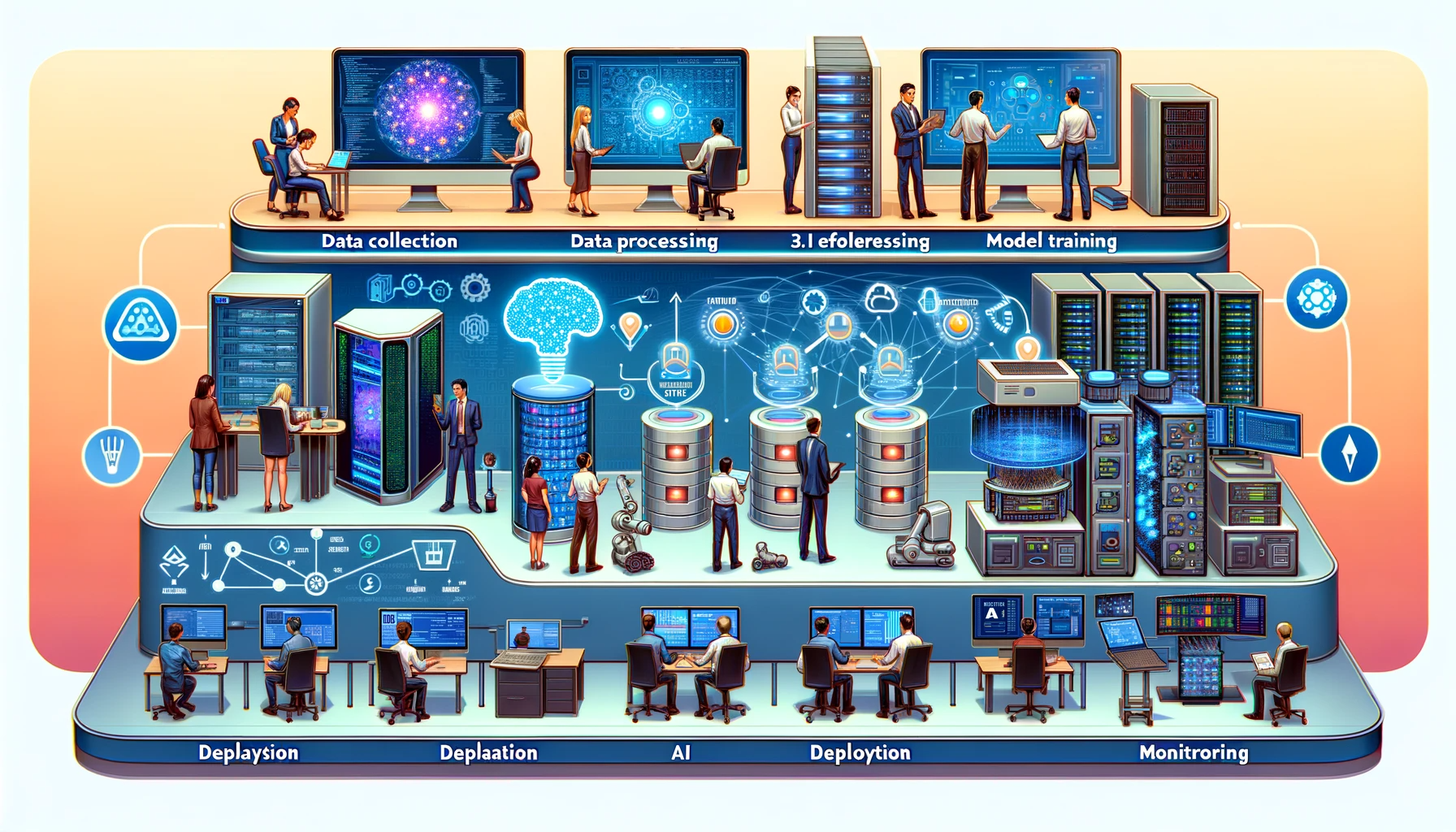
Purpose
-------
_Why do machine learning prototypes that work perfectly in development often fail catastrophically when deployed to production environments?_
The transition from prototype models to reliable production systems presents significant engineering challenges. Research models trained on clean datasets encounter production environments with shifting data distributions, evolving user behaviors, and unexpected system failures. Unlike traditional software that executes deterministic logic, machine learning systems exhibit probabilistic behavior that degrades silently as real-world conditions diverge from training assumptions. This instability requires operational practices that detect performance degradation before affecting users, automatically retrain models as data evolves, and maintain system reliability despite prediction uncertainty. Success demands engineering disciplines that bridge experimental validation and production reliability, enabling organizations to deploy models that remain effective throughout their operational lifespan.
Learning Objectives
* Differentiate between traditional software failures and ML system silent failures to explain why MLOps emerged as a distinct engineering discipline
* Analyze technical debt patterns (boundary erosion, correction cascades, data dependencies) in ML systems and propose systematic engineering solutions
* Design CI/CD pipelines that address ML-specific challenges including model validation, data versioning, and automated retraining workflows
* Evaluate monitoring strategies for production ML systems that detect both traditional system metrics and ML-specific indicators like data drift and prediction confidence
* Implement deployment patterns for diverse environments including cloud services, edge devices, and federated learning systems
* Assess organizational maturity levels for effective MLOps implementation
* Compare MLOps adaptations across domains by analyzing how specialized requirements (healthcare, embedded systems) reshape operational frameworks
* Create governance frameworks that ensure model reproducibility, auditability, and compliance in regulated environments
Introduction to Machine Learning Operations
-------------------------------------------
Traditional software fails loudly with error messages and stack traces; machine learning systems fail silently. As introduced in **[Chapter 1: Introduction](https://mlsysbook.ai/contents/core/introduction/introduction.html#sec-introduction)
**, the Silent Failure Problem is a defining characteristic of ML systems: performance degrades gradually as data distributions shift, user behaviors evolve, and model assumptions become outdated, all without raising any alarms. MLOps is the engineering discipline designed to make those silent failures visible and manageable. It provides the monitoring, automation, and governance required to ensure that data-driven systems remain reliable in production, even as the world around them changes.
Machine learning systems require more than algorithmic innovation; they need systematic engineering practices for reliable production deployment. While **[Chapter 14: On-Device Learning](https://mlsysbook.ai/contents/core/ondevice_learning/ondevice_learning.html#sec-ondevice-learning)
** explored distributed learning under resource constraints and **[Chapter 16: Robust AI](https://mlsysbook.ai/contents/core/robust_ai/robust_ai.html#sec-robust-ai)
** established fault tolerance methodologies, the security framework from **[Chapter 15: Security & Privacy](https://mlsysbook.ai/contents/core/privacy_security/privacy_security.html#sec-security-privacy)
** becomes essential for production deployment. Machine Learning Operations (MLOps)[1](https://mlsysbook.ai/contents/core/ops/ops.html#fn1)
provides the disciplinary framework that synthesizes these specialized capabilities into coherent production architectures. This operational discipline addresses the challenge of translating experimental success into sustainable system performance, integrating adaptive learning, security protocols, and resilience mechanisms within complex production ecosystems.
1 **MLOps Emergence**: While machine learning operations challenges were identified earlier by D. Sculley and colleagues at Google in their influential 2015 paper “Hidden Technical Debt in Machine Learning Systems” ([Sculley et al. 2021](https://mlsysbook.ai/contents/core/ops/ops.html#ref-sculley2015hidden)
), the term “MLOps” itself was coined around 2018 as the discipline matured. The field emerged as organizations like Netflix, Uber, and Airbnb faced the “last mile” problem, where approximately 90% of ML models never made it to production according to industry surveys and anecdotal reports due to operational challenges.
Sculley, D., G. Holt, D. Golovin, E. Davydov, T. Phillips, D. Ebner, V. Chaudhary, M. Young, J. F. Crespo, and D. Dennison. 2021. “Technical Debt in Machine Learning Systems.” In _Technical Debt in Practice_, 28:177–92. The MIT Press. [https://doi.org/10.7551/mitpress/12440.003.0011](https://doi.org/10.7551/mitpress/12440.003.0011)
.
MLOps ([Section 1.2.2](https://mlsysbook.ai/contents/core/ops/ops.html#sec-ml-operations-mlops-c12b)
) systematically integrates machine learning methodologies, data science practices, and software engineering principles to enable automated, end-to-end lifecycle management. This operational paradigm bridges experimental validation and production deployment, ensuring that validated models maintain their performance characteristics while adapting to real-world operational environments.
Consider deploying a demand prediction system for ridesharing services. While controlled experimental validation may demonstrate superior accuracy and latency characteristics, production deployment introduces challenges that extend beyond algorithmic performance. Data streams exhibit varying quality, temporal patterns undergo seasonal variations, and prediction services must satisfy strict availability requirements while maintaining real-time response capabilities. MLOps provides the framework needed to address these operational complexities.
As an engineering discipline, MLOps establishes standardized protocols, tools, and workflows that facilitate the transition of validated models from experimental environments to production systems. The discipline promotes collaboration by formalizing interfaces and defining responsibilities across traditionally isolated domains, including data science, machine learning engineering, and systems operations[2](https://mlsysbook.ai/contents/core/ops/ops.html#fn2)
. This approach enables continuous integration and deployment practices adapted for machine learning contexts, supporting iterative model refinement, validation, and deployment while preserving system stability and operational reliability.
2 **DevOps Origins**: The “wall of confusion” between development and operations teams was so notorious that Patrick Debois called his 2009 conference “DevOpsDays” specifically to bridge this gap. The movement emerged from the frustrations of the “throw it over the wall” mentality where developers built software in isolation from operations teams who had to deploy and maintain it.
Building on these operational foundations, mature MLOps methodologies transform how organizations manage machine learning systems through automation and monitoring frameworks. These practices enable continuous model retraining as new data becomes available, evaluation of alternative architectures against production baselines, controlled deployment of experimental modifications through graduated rollout strategies, and real-time performance assessment without compromising operational continuity. This operational flexibility ensures sustained model relevance while maintaining system reliability standards.
Beyond operational efficiency, MLOps encompasses governance frameworks and accountability mechanisms that become critical as systems scale. MLOps standardizes the tracking of model versions, data lineage documentation, and configuration parameter management, establishing reproducible and auditable artifact trails. This rigor proves essential in regulated domains where model interpretability and operational provenance constitute compliance requirements.
The practical benefits of this methodological rigor become evident in organizational outcomes. Evidence demonstrates that organizations adopting mature MLOps methodologies achieve significant improvements in deployment reliability, accelerated time-to-market cycles, and enhanced system maintainability[3](https://mlsysbook.ai/contents/core/ops/ops.html#fn3)
. The disciplinary framework enables sustainable scaling of machine learning systems while preserving the performance characteristics validated during benchmarking phases, ensuring operational fidelity to experimental results.
3 **MLOps Business Impact**: Companies implementing mature MLOps practices report significant improvements in deployment speed (reducing time from months to weeks), substantial reductions in model debugging time, and improved model reliability. Organizations with mature MLOps practices consistently achieve higher model success rates moving from pilot to production compared to those using ad hoc approaches.
This methodology of machine learning operations provides the pathway for transforming theoretical innovations into sustainable production capabilities. This chapter establishes the engineering foundations needed to bridge the gap between experimentally validated systems and operationally reliable production deployments. The analysis focuses particularly on centralized cloud computing environments, where monitoring infrastructure and management capabilities enable the implementation of mature operational practices for large-scale machine learning systems.
While **[Chapter 10: Model Optimizations](https://mlsysbook.ai/contents/core/optimizations/optimizations.html#sec-model-optimizations)
** and **[Chapter 9: Efficient AI](https://mlsysbook.ai/contents/core/efficient_ai/efficient_ai.html#sec-efficient-ai)
** establish optimization foundations, this chapter extends these techniques to production contexts requiring continuous maintenance and monitoring. The empirical benchmarking approaches established in **[Chapter 12: Benchmarking AI](https://mlsysbook.ai/contents/core/benchmarking/benchmarking.html#sec-benchmarking-ai)
** provide the methodological foundation for production performance assessment, while system reliability patterns emerge as critical determinants of operational availability. MLOps integrates these diverse technical foundations into unified operational workflows, systematically addressing the fundamental challenge of transitioning from model development to sustainable production deployment.
This chapter examines the theoretical foundations and practical motivations underlying MLOps, traces its disciplinary evolution from DevOps methodologies, and identifies the principal challenges and established practices that inform its adoption in contemporary machine learning system architectures.
**Self-Check: Question 1.1**
1. What is the Silent Failure Problem in machine learning systems?
1. A sudden crash of the system with error messages.
2. Gradual performance degradation without noticeable alerts.
3. A complete failure of the model to make predictions.
4. An increase in computational resource usage.
2. How does MLOps address the Silent Failure Problem in machine learning systems?
3. Which of the following best describes the role of MLOps in machine learning system deployment?
1. It provides a framework for automated, end-to-end lifecycle management.
2. It focuses solely on algorithmic innovation.
3. It is concerned only with the security of machine learning models.
4. It replaces the need for data science practices.
4. Consider a scenario where a ridesharing service is deploying a demand prediction system. What are some operational challenges that MLOps can help address in this context?
[See Answers →](https://mlsysbook.ai/contents/core/ops/ops.html#quiz-answer-sec-ml-operations-introduction-machine-learning-operations-5f4b)
Historical Context
------------------
Understanding this evolution from DevOps to MLOps clarifies why traditional operational practices require adaptation for machine learning systems. The following examination of this historical development reveals the specific challenges that motivated MLOps as a distinct discipline.
MLOps has its roots in DevOps, a set of practices that combines software development (Dev) and IT operations (Ops) to shorten the development lifecycle and support the continuous delivery of high-quality software. DevOps and MLOps both emphasize automation, collaboration, and iterative improvement. However, while DevOps emerged to address challenges in software deployment and operational management, MLOps evolved in response to the unique complexities of machine learning workflows, especially those involving data-driven components ([Breck et al. 2017](https://mlsysbook.ai/contents/core/ops/ops.html#ref-breck2020ml)
). Understanding this evolution is important for appreciating the motivations and structure of modern ML systems.
Breck, Eric, Shanqing Cai, Eric Nielsen, Michael Salib, and D. Sculley. 2017. “The ML Test Score: A Rubric for ML Production Readiness and Technical Debt Reduction.” In _2017 IEEE International Conference on Big Data (Big Data)_, 6:1123–32. 2. IEEE. [https://doi.org/10.1109/bigdata.2017.8258038](https://doi.org/10.1109/bigdata.2017.8258038)
.
### DevOps
The term DevOps was coined in 2009 by [Patrick Debois](https://www.jedi.be/)
, a consultant and Agile practitioner who organized the first [DevOpsDays](https://www.devopsdays.org/)
conference in Ghent, Belgium. DevOps extended the principles of the [Agile](https://agilemanifesto.org/)
movement, that emphasized close collaboration among development teams and rapid, iterative releases, by bringing IT operations into the fold.
This innovation addressed a core problem in traditional software pipelines, where development and operations teams worked in silos, creating inefficiencies, delays, and misaligned priorities. DevOps emerged as a response, advocating shared ownership, infrastructure as code[4](https://mlsysbook.ai/contents/core/ops/ops.html#fn4)
, and automation to streamline deployment pipelines.
4 **Infrastructure as Code**: The concept emerged from the painful lessons of “snowflake servers”, unique, manually-configured systems that were impossible to reproduce. Luke Kanies created Puppet in 2005 after experiencing the nightmare of managing hundreds of custom-configured servers at various startups.
5 **Jenkins Origins**: Originally called “Hudson,” Jenkins was created by Kohsuke Kawaguchi at Sun Microsystems in 2004 to automate his own tedious testing processes. The name change to “Jenkins” came in 2011 after a trademark dispute, named after the devoted butler from P.G. Wodehouse’s stories.
6 **Kubernetes Origins**: Greek for “helmsman,” Kubernetes emerged from Google’s internal Borg system that managed billions of containers across their data centers. Google open-sourced it in 2014, realizing that their competitive advantage wasn’t the orchestration system itself, but how they used it to run services at planetary scale.
7 **Containerization and Orchestration**: Docker containers package applications with all their dependencies into standardized, portable units that run consistently across different computing environments, isolating software from infrastructure variations. Kubernetes orchestrates these containers at scale, automating deployment, load balancing, scaling, and recovery across clusters of machines. Together, they enable the reproducible, automated infrastructure management essential for modern MLOps, where models and their serving environments must be deployed consistently across development, staging, and production.
To support these principles, tools such as [Jenkins](https://www.jenkins.io/)
[5](https://mlsysbook.ai/contents/core/ops/ops.html#fn5)
, [Docker](https://www.docker.com/)
, and [Kubernetes](https://kubernetes.io/)
[6](https://mlsysbook.ai/contents/core/ops/ops.html#fn6)
[7](https://mlsysbook.ai/contents/core/ops/ops.html#fn7)
became foundational for implementing continuous integration and continuous delivery (CI/CD) practices.
Through automation and feedback loops, DevOps promotes collaboration while reducing time-to-release and improving software reliability. This success established the cultural and technical groundwork for extending similar principles to the ML domain.
### MLOps
While DevOps achieved considerable success in traditional software deployment, machine learning systems introduced new challenges that required further adaptation. MLOps builds on the DevOps foundation but addresses the specific demands of ML system development and deployment. Where DevOps focuses on integrating and delivering deterministic software, MLOps must manage non-deterministic, data-dependent workflows. These workflows span data acquisition, preprocessing, model training, evaluation, deployment, and continuous monitoring (see [Figure 1](https://mlsysbook.ai/contents/core/ops/ops.html#fig-mlops-diagram)
).
**Definition:** MLOps
**_Machine Learning Operations (MLOps)_** is the engineering discipline that manages the _end-to-end lifecycle_ of machine learning systems in production, addressing the unique challenges of _data versioning_, _model evolution_, and _continuous retraining_.
The operational complexity and business risk of deploying machine learning without systematic engineering practices becomes clear when examining real-world failures. Consider a retail company that deployed a recommendation model that initially boosted sales by 15%. However, due to a silent data drift issue, the model’s accuracy degraded over six months, eventually reducing sales by 5% compared to the original system. The problem went undetected because monitoring focused on system uptime rather than model performance metrics. The company lost an estimated $10 million in revenue before the issue was discovered during routine quarterly analysis. This scenario, common in early ML deployments, illustrates why MLOps, with its emphasis on continuous model monitoring and automated retraining, is not merely an engineering best practice, but a business necessity for organizations depending on machine learning systems for critical operations.
This adaptation was driven by several recurring challenges in operationalizing machine learning that distinguished it from traditional software deployment. Data drift[8](https://mlsysbook.ai/contents/core/ops/ops.html#fn8)
, where shifts in input data distributions over time degrade model accuracy, requires continuous monitoring and automated retraining procedures.
8 **Data Drift Discovery**: The concept was first formalized by researchers studying spam detection systems in the early 2000s, who noticed that spam patterns evolved so rapidly that models became obsolete within weeks. This led to the realization that ML systems face a different challenge than traditional software: their environment actively adapts to defeat them.
9 **ML Reproducibility Crisis**: A 2016 study by Collberg and Proebsting found that only 54% of computer systems research papers could be reproduced even when authors were available to assist ([Collberg and Proebsting 2016](https://mlsysbook.ai/contents/core/ops/ops.html#ref-collberg2016repeatability)
). This reproducibility challenge is even more acute in ML research, though the situation has improved with initiatives like Papers with Code and requirements for code submission at major ML conferences.
Collberg, Christian, and Todd A. Proebsting. 2016. “Repeatability in Computer Systems Research.” _Communications of the ACM_ 59 (3): 62–69. [https://doi.org/10.1145/2812803](https://doi.org/10.1145/2812803)
.
Schelter, Sebastian, Matthias Boehm, Johannes Kirschnick, Kostas Tzoumas, and Gunnar Ratsch. 2018. “Automating Large-Scale Machine Learning Model Management.” In _Proceedings of the 2018 IEEE International Conference on Data Engineering (ICDE)_, 137–48. IEEE.
Building on this data-centric challenge, reproducibility[9](https://mlsysbook.ai/contents/core/ops/ops.html#fn9)
presents another issue. ML workflows lack standardized mechanisms to track code, datasets, configurations, and environments, making it difficult to reproduce past experiments ([Schelter et al. 2018](https://mlsysbook.ai/contents/core/ops/ops.html#ref-schelter2018automating)
). The lack of explainability in complex models has driven demand for tools that increase model transparency and interpretability, particularly in regulated domains.
[](https://mlsysbook.ai/contents/core/ops/9db7c8e7810e5d1080dec551cdee1ff0e7d4dffe.svg "Figure 1: MLOps Lifecycle: MLOps extends DevOps principles to manage the unique challenges of machine learning systems, including data versioning, model retraining, and continuous monitoring. This diagram outlines the iterative workflow encompassing data engineering, model development, and reliable deployment for sustained performance in production.")
Figure 1: **MLOps Lifecycle**: MLOps extends DevOps principles to manage the unique challenges of machine learning systems, including data versioning, model retraining, and continuous monitoring. This diagram outlines the iterative workflow encompassing data engineering, model development, and reliable deployment for sustained performance in production.
Beyond these foundational challenges, organizations face additional operational complexities. Post-deployment monitoring of model performance proves difficult, especially in detecting silent failures or changes in user behavior. The manual overhead involved in retraining and redeploying models creates friction in experimentation and iteration. Configuring and maintaining ML infrastructure is complex and error-prone, highlighting the need for platforms that offer optimized, modular, and reusable infrastructure. Together, these challenges form the foundation for MLOps practices that focus on automation, collaboration, and lifecycle management.
In response to these distinct challenges, the field developed specialized tools and workflows tailored to the ML lifecycle. Building on DevOps foundations while addressing ML-specific requirements, MLOps coordinates a broader stakeholder ecosystem and introduces specialized practices such as data versioning[10](https://mlsysbook.ai/contents/core/ops/ops.html#fn10)
, model versioning, and model monitoring that extend beyond traditional DevOps scope. These practices are detailed in [Table 1](https://mlsysbook.ai/contents/core/ops/ops.html#tbl-mlops)
:
10 **DVC Creation Story**: Data Version Control was born from the frustration of Dmitry Petrov, who spent weeks trying to reproduce an experiment only to discover the training data had been quietly updated. He created DVC in 2017 to bring Git-like versioning to data science, solving what he called “the biggest unsolved problem in machine learning.”
Table 1: **MLOps vs. DevOps**: MLOps extends DevOps principles to address the unique requirements of machine learning systems, including data and model versioning, and continuous monitoring for model performance and data drift. This table clarifies how MLOps coordinates a broader range of stakeholders and emphasizes reproducibility and scalability beyond traditional software development workflows.
| | | |
| --- | --- | --- |
| **Objective** | Streamlining software development and operations processes | Optimizing the lifecycle of machine learning models |
| **Methodology** | Continuous Integration and Continuous Delivery (CI/CD) for software development | Similar to CI/CD but focuses on machine learning workflows |
| **Primary Tools** | Version control (Git), CI/CD tools (Jenkins, Travis CI), Configuration management (Ansible, Puppet) | Data versioning tools, Model training and deployment tools, CI/CD pipelines tailored for ML |
| **Primary Concerns** | Code integration, Testing, Release management, Automation, Infrastructure as code | Data management, Model versioning, Experiment tracking, Model deployment, Scalability of ML workflows |
| **Typical Outcomes** | Faster and more reliable software releases, Improved collaboration between development and operations teams | Efficient management and deployment of machine learning models, Enhanced collaboration between data scientists and engineers |
With these foundational distinctions established, we must first understand the unique operational challenges that motivate sophisticated MLOps practices before examining the infrastructure and practices designed to address them.
**Self-Check: Question 1.2**
1. What was the primary motivation for the evolution from DevOps to MLOps?
1. To address the unique complexities of machine learning workflows
2. To improve software deployment speeds
3. To enhance collaboration between developers and IT operations
4. To reduce costs in software development
2. Explain how the concept of ‘Infrastructure as Code’ contributed to the development of DevOps practices.
3. Which of the following is a key difference between DevOps and MLOps?
1. DevOps and MLOps both focus on data versioning.
2. DevOps emphasizes model versioning, whereas MLOps does not.
3. DevOps focuses on deterministic software, while MLOps manages non-deterministic workflows.
4. MLOps is primarily concerned with software release management.
4. In a production system, how might MLOps practices prevent issues like the silent data drift problem described in the section?
[See Answers →](https://mlsysbook.ai/contents/core/ops/ops.html#quiz-answer-sec-ml-operations-historical-context-8f3a)
Technical Debt and System Complexity
------------------------------------
While the DevOps foundation provides automation and collaboration principles, machine learning systems introduce unique forms of complexity that require engineering approaches to manage effectively. Unlike traditional software where broken code fails immediately, ML systems can degrade silently through data changes, model interactions, and evolving requirements. While federated learning systems face unique coordination challenges (**[Chapter 14: On-Device Learning](https://mlsysbook.ai/contents/core/ondevice_learning/ondevice_learning.html#sec-ondevice-learning)
**) and robust systems require careful monitoring (**[Chapter 16: Robust AI](https://mlsysbook.ai/contents/core/robust_ai/robust_ai.html#sec-robust-ai)
**), all deployment contexts must balance operational efficiency with security requirements. Understanding these operational challenges, collectively known as technical debt, is essential for motivating the engineering solutions and practices that follow.
This complexity manifests as machine learning systems mature and scale, where they accumulate technical debt: the long-term cost of expedient design decisions made during development. Originally proposed in software engineering in the 1990s[11](https://mlsysbook.ai/contents/core/ops/ops.html#fn11)
, this metaphor compares shortcuts in implementation to financial debt: it may enable short-term velocity, but requires ongoing interest payments in the form of maintenance, refactoring, and systemic risk.
11 **Technical Debt Origins**: Ward Cunningham coined the term in 1992, comparing rushed coding decisions to financial debt: “A little debt speeds development so long as it is paid back promptly with a rewrite.” He later regretted the metaphor became an excuse for bad code rather than a tool for communicating tradeoffs.
[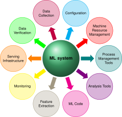](https://mlsysbook.ai/contents/core/ops/ad41dbbec59c26670e88f85c2ecc020a960b3dc8.svg "Figure 2: ML System Complexity: Most engineering effort in a typical machine learning system concentrates on components surrounding the model itself (data collection, feature engineering, and system configuration) rather than the model code. This distribution underscores the operational challenges and potential for technical debt arising from these often-overlooked areas of an ML system. Source: [@sculley2015hidden].")
Figure 2: **ML System Complexity**: Most engineering effort in a typical machine learning system concentrates on components surrounding the model itself (data collection, feature engineering, and system configuration) rather than the model code. This distribution underscores the operational challenges and potential for technical debt arising from these often-overlooked areas of an ML system. Source: ([Sculley et al. 2021](https://mlsysbook.ai/contents/core/ops/ops.html#ref-sculley2015hidden)
).
These operational challenges manifest in several distinct patterns that teams encounter as their ML systems evolve. Rather than cataloging every debt pattern, we focus on representative examples that illustrate the engineering approaches MLOps provides. Each challenge emerges from unique characteristics of machine learning workflows: their reliance on data rather than deterministic logic, their statistical rather than exact behavior, and their tendency to create implicit dependencies through data flows rather than explicit interfaces.
The following technical debt patterns demonstrate why traditional DevOps practices require extension for ML systems, motivating the infrastructure solutions presented in subsequent sections.
Building on this systems perspective, we examine key categories of technical debt unique to ML systems ([Figure 3](https://mlsysbook.ai/contents/core/ops/ops.html#fig-technical-debt-taxonomy)
). Each subsection highlights common sources, illustrative examples, and engineering solutions that address these challenges. While some forms of debt may be unavoidable during early development, understanding their causes and impact enables engineers to design robust and maintainable ML systems through disciplined architectural practices and appropriate tooling choices.
[](https://mlsysbook.ai/contents/core/ops/f3ed518d855126d9d8cd324e3fbfa1da69e12d78.svg "Figure 3: ML Technical Debt Taxonomy: Machine learning systems accumulate distinct forms of technical debt that emerge from data dependencies, model interactions, and evolving requirements. This hub-and-spoke diagram illustrates the primary debt patterns: boundary erosion undermines modularity, correction cascades propagate fixes through dependencies, feedback loops create hidden coupling, while data, configuration, and pipeline debt reflect poorly managed artifacts and workflows. Understanding these patterns enables systematic engineering approaches to debt prevention and mitigation.")
Figure 3: **ML Technical Debt Taxonomy**: Machine learning systems accumulate distinct forms of technical debt that emerge from data dependencies, model interactions, and evolving requirements. This hub-and-spoke diagram illustrates the primary debt patterns: boundary erosion undermines modularity, correction cascades propagate fixes through dependencies, feedback loops create hidden coupling, while data, configuration, and pipeline debt reflect poorly managed artifacts and workflows. Understanding these patterns enables systematic engineering approaches to debt prevention and mitigation.
### Boundary Erosion
In traditional software systems, modularity and abstraction provide clear boundaries between components, allowing changes to be isolated and behavior to remain predictable. Machine learning systems, in contrast, tend to blur these boundaries. The interactions between data pipelines, feature engineering, model training, and downstream consumption often lead to tightly coupled components with poorly defined interfaces.
This erosion of boundaries makes ML systems particularly vulnerable to cascading effects from even minor changes. A seemingly small update to a preprocessing step or feature transformation can propagate through the system in unexpected ways, breaking assumptions made elsewhere in the pipeline. This lack of encapsulation increases the risk of entanglement, where dependencies between components become so intertwined that local modifications require global understanding and coordination.
One manifestation of this problem is known as CACHE (Change Anything Changes Everything). When systems are built without strong boundaries, adjusting a feature encoding, model hyperparameter, or data selection criterion can affect downstream behavior in unpredictable ways. This inhibits iteration and makes testing and validation more complex. For example, changing the binning strategy of a numerical feature may cause a previously tuned model to underperform, triggering retraining and downstream evaluation changes.
To mitigate boundary erosion, teams should prioritize architectural practices that support modularity and encapsulation. Designing components with well-defined interfaces allows teams to isolate faults, reason about changes, and reduce the risk of system-wide regressions. For instance, clearly separating data ingestion from feature engineering, and feature engineering from modeling logic, introduces layers that can be independently validated, monitored, and maintained.
Boundary erosion is often invisible in early development but becomes a significant burden as systems scale or require adaptation. However, established software engineering practices can effectively prevent and mitigate this problem. Proactive design decisions that preserve abstraction and limit interdependencies, combined with systematic testing and interface documentation, provide practical solutions for managing complexity and avoiding long-term maintenance costs.
This challenge arises because ML systems operate with statistical rather than logical guarantees, making traditional software engineering boundaries harder to enforce. Understanding why boundary erosion occurs so frequently requires examining how machine learning workflows differ from conventional software development.
Boundary erosion in ML systems violates established software engineering principles, particularly the Law of Demeter and the principle of least knowledge. While traditional software achieves modularity through explicit interfaces and information hiding, ML systems create implicit couplings through data flows that bypass these explicit boundaries.
The CACHE phenomenon represents a breakdown of the Liskov Substitution Principle, where component modifications violate behavioral contracts expected by dependent components. Unlike traditional software with compile-time guarantees, ML systems operate with statistical behavior that creates inherently different coupling patterns.
The challenge lies in reconciling traditional modularity concepts with the inherently interconnected nature of ML workflows, where statistical dependencies and data-driven behavior create coupling patterns that traditional software engineering frameworks were not designed to handle.
### Correction Cascades
As machine learning systems evolve, they often undergo iterative refinement to address performance issues, accommodate new requirements, or adapt to environmental changes. In well-engineered systems, such updates are localized and managed through modular changes. However, in ML systems, even small adjustments can trigger correction cascades, a sequence of dependent fixes that propagate backward and forward through the workflow.
The diagram in [Figure 4](https://mlsysbook.ai/contents/core/ops/ops.html#fig-correction-cascades-flowchart)
visualizes how these cascading effects propagate through ML system development. Understanding the structure of these cascades helps teams anticipate and mitigate their impact.
[Figure 4](https://mlsysbook.ai/contents/core/ops/ops.html#fig-correction-cascades-flowchart)
illustrates how these cascades emerge across different stages of the ML lifecycle, from problem definition and data collection to model development and deployment. Each arc represents a corrective action, and the colors indicate different sources of instability, including inadequate domain expertise, brittle real-world interfaces, misaligned incentives, and insufficient documentation. The red arrows represent cascading revisions, while the dotted arrow at the bottom highlights a full system restart, a drastic but sometimes necessary outcome.
[](https://mlsysbook.ai/contents/core/ops/42e7fff97c3a3c84a75ca00f3e1adc11fddbd994.svg "Figure 4: Correction Cascades: Iterative refinements in ML systems often trigger dependent fixes across the workflow, propagating from initial adjustments through data, model, and deployment stages. Color-coded arcs represent corrective actions stemming from sources of instability, while red arrows and the dotted line indicate escalating revisions, potentially requiring a full system restart.")
Figure 4: **Correction Cascades**: Iterative refinements in ML systems often trigger dependent fixes across the workflow, propagating from initial adjustments through data, model, and deployment stages. Color-coded arcs represent corrective actions stemming from sources of instability, while red arrows and the dotted line indicate escalating revisions, potentially requiring a full system restart.
One common source of correction cascades is sequential model development: reusing or fine-tuning existing models to accelerate development for new tasks. While this strategy is often efficient, it can introduce hidden dependencies that are difficult to unwind later. Assumptions baked into earlier models become implicit constraints for future models, limiting flexibility and increasing the cost of downstream corrections.
Consider a scenario where a team fine-tunes a customer churn prediction model for a new product. The original model may embed product-specific behaviors or feature encodings that are not valid in the new setting. As performance issues emerge, teams may attempt to patch the model, only to discover that the true problem lies several layers upstream, perhaps in the original feature selection or labeling criteria.
To avoid or reduce the impact of correction cascades, teams must make careful tradeoffs between reuse and redesign. Several factors influence this decision. For small, static datasets, fine-tuning may be appropriate. For large or rapidly evolving datasets, retraining from scratch provides greater control and adaptability. Fine-tuning also requires fewer computational resources, making it attractive in constrained settings. However, modifying foundational components later becomes extremely costly due to these cascading effects.
Therefore, careful consideration should be given to introducing fresh model architectures, even if resource-intensive, to avoid correction cascades down the line. This approach may help mitigate the amplifying effects of issues downstream and reduce technical debt. However, there are still scenarios where sequential model building makes sense, necessitating a thoughtful balance between efficiency, flexibility, and long-term maintainability in the ML development process.
To understand why correction cascades occur so persistently in ML systems despite best practices, it helps to examine the underlying mechanisms that drive this phenomenon. The correction cascade pattern emerges from hidden feedback loops that violate system modularity principles established in software engineering. When model A’s outputs influence model B’s training data, this creates implicit dependencies that undermine modular design. These dependencies are particularly insidious because they operate through data flows rather than explicit code interfaces, making them invisible to traditional dependency analysis tools.
From a systems theory perspective, correction cascades represent instances of tight coupling between supposedly independent components. The cascade propagation follows power-law distributions, where small initial changes can trigger disproportionately large system-wide modifications. This phenomenon parallels the butterfly effect in complex systems, where minor perturbations amplify through nonlinear interactions.
Understanding these theoretical foundations helps engineers recognize that preventing correction cascades requires not just better tooling, but architectural decisions that preserve system modularity even in the presence of learning components. The challenge lies in designing ML systems that maintain loose coupling despite the inherently interconnected nature of data-driven workflows.
### Interface and Dependency Challenges
Unlike traditional software where component interactions occur through explicit APIs, ML systems often develop implicit dependencies through data flows and shared outputs. Two critical patterns illustrate these challenges:
**Undeclared Consumers**: Model outputs frequently serve downstream components without formal tracking or interface contracts. When models evolve, these hidden dependencies can break silently. For example, a credit scoring model’s outputs might feed an eligibility engine, which influences future applicant pools and training data, creating untracked feedback loops that bias model behavior over time.
**Data Dependency Debt**: ML pipelines accumulate unstable and underutilized data dependencies that become difficult to trace or validate. Feature engineering scripts, data joins, and labeling conventions lack the dependency analysis tools available in traditional software development. When data sources change structure or distribution, downstream models can fail unexpectedly.
**Engineering Solutions**: These challenges require systematic approaches including strict access controls for model outputs, formal interface contracts with documented schemas, data versioning and lineage tracking systems, and comprehensive monitoring of prediction usage patterns. The MLOps infrastructure patterns presented in subsequent sections provide concrete implementations of these solutions.
### System Evolution Challenges
As ML systems mature, they face unique evolution challenges that differ fundamentally from traditional software:
**Feedback Loops**: Models influence their own future behavior through the data they generate. Recommendation systems exemplify this: suggested items shape user clicks, which become training data, potentially creating self-reinforcing biases. These loops undermine data independence assumptions and can mask performance degradation for months.
**Pipeline and Configuration Debt**: ML workflows often evolve into “pipeline jungles” of ad hoc scripts and fragmented configurations. Without modular interfaces, teams build duplicate pipelines rather than refactor brittle ones, leading to inconsistent processing and maintenance burden.
**Early-Stage Shortcuts**: Rapid prototyping encourages embedding business logic in training code and undocumented configuration changes. While necessary for innovation, these shortcuts become liabilities as systems scale across teams.
**Engineering Solutions**: Managing evolution requires architectural discipline including cohort-based monitoring for loop detection, modular pipeline design with workflow orchestration tools, and treating configuration as a first-class system component with versioning and validation.
### Real-World Technical Debt Examples
Hidden technical debt is not just theoretical; it has played a critical role in shaping the trajectory of real-world machine learning systems. These examples illustrate how unseen dependencies and misaligned assumptions can accumulate quietly, only to become major liabilities over time:
#### YouTube: Feedback Loop Debt
YouTube’s recommendation engine has faced repeated criticism for promoting sensational or polarizing content[12](https://mlsysbook.ai/contents/core/ops/ops.html#fn12)
. A large part of this stems from feedback loop debt: recommendations influence user behavior, which in turn becomes training data. Over time, this led to unintended content amplification. Mitigating this required substantial architectural overhauls, including cohort-based evaluation, delayed labeling, and more explicit disentanglement between engagement metrics and ranking logic.
12 **YouTube Recommendation Impact**: The recommendation system drives 70% of watch time on the platform (1+ billion hours daily), but algorithmic changes in 2016 increased average session time by 50% while inadvertently promoting conspiracy content. Fixing these feedback loops required 2+ years of engineering work and new evaluation frameworks.
#### Zillow: Correction Cascade Failure
Zillow’s home valuation model (Zestimate) faced significant correction cascades during its iBuying venture[13](https://mlsysbook.ai/contents/core/ops/ops.html#fn13)
. When initial valuation errors propagated into purchasing decisions, retroactive corrections triggered systemic instability that required data revalidation, model redesign, and eventually a full system rollback. The company shut down the iBuying arm in 2021, citing model unpredictability and data feedback effects as core challenges.
13 **Zillow iBuying Failure**: Zillow lost $881 million in a single quarter (Q3 2021) due to multiple factors including ML model failures, with the Zestimate algorithm reportedly overvaluing homes by an average of 5-7%. The company laid off 2,000+ employees and took a $569 million inventory write-down when shutting down Zillow Offers.
#### Tesla: Undeclared Consumer Debt
In early deployments, Tesla’s Autopilot made driving decisions based on models whose outputs were repurposed across subsystems without clear boundaries. Over-the-air updates occasionally introduced silent behavior changes that affected multiple subsystems (e.g., lane centering and braking) in unpredictable ways. This entanglement illustrates undeclared consumer debt and the risks of skipping strict interface governance in ML-enabled safety-critical systems.
#### Facebook: Configuration Debt
Facebook’s News Feed algorithm has undergone numerous iterations, often driven by rapid experimentation. However, the lack of consistent configuration management led to opaque settings that influenced content ranking without clear documentation. As a result, changes to the algorithm’s behavior were difficult to trace, and unintended consequences emerged from misaligned configurations. This situation highlights the importance of treating configuration as a first-class citizen in ML systems.
These real-world examples demonstrate the pervasive nature of technical debt in ML systems and why traditional DevOps practices require systematic extension. The infrastructure and production operations sections that follow present concrete engineering solutions designed to address these specific challenges: feature stores address data dependency debt, versioning systems enable reproducible configurations, monitoring frameworks detect feedback loops, and modular pipeline architectures prevent technical debt accumulation. This understanding of operational challenges provides the essential motivation for the specialized MLOps tools and practices we examine next.
**Self-Check: Question 1.3**
1. What is a primary cause of boundary erosion in machine learning systems?
1. Explicit interfaces between components
2. Strong modularity and encapsulation
3. Statistical rather than logical guarantees
4. Comprehensive testing and validation
2. Explain how correction cascades can affect the lifecycle of a machine learning system.
3. Which of the following best describes the CACHE principle in ML systems?
1. A method to cache intermediate results to improve efficiency
2. A principle for optimizing computational resources
3. A strategy for efficient data storage and retrieval
4. A phenomenon where any change can affect the entire system
4. Order the following stages to illustrate the propagation of correction cascades in an ML system: (1) Model training, (2) Data collection, (3) Model deployment, (4) Model evaluation.
5. In a production system, how might you address undeclared consumer debt to improve system reliability?
[See Answers →](https://mlsysbook.ai/contents/core/ops/ops.html#quiz-answer-sec-ml-operations-technical-debt-system-complexity-0bb6)
Development Infrastructure and Automation
-----------------------------------------
Building on the operational challenges established above, this section examines the infrastructure and development components that enable the specialized capabilities from preceding chapters while addressing systemic challenges. These foundational components must support federated learning coordination for edge devices (**[Chapter 14: On-Device Learning](https://mlsysbook.ai/contents/core/ondevice_learning/ondevice_learning.html#sec-ondevice-learning)
**), implement secure model serving with privacy guarantees (**[Chapter 15: Security & Privacy](https://mlsysbook.ai/contents/core/privacy_security/privacy_security.html#sec-security-privacy)
**), and maintain robustness monitoring for distribution shifts (**[Chapter 16: Robust AI](https://mlsysbook.ai/contents/core/robust_ai/robust_ai.html#sec-robust-ai)
**). They form a layered architecture, as illustrated in Figure [Figure 5](https://mlsysbook.ai/contents/core/ops/ops.html#fig-ops-layers)
, that integrates these diverse requirements into a cohesive operational framework. Understanding how these components interact enables practitioners to design systems that simultaneously achieve edge efficiency, security compliance, and fault tolerance while maintaining operational sustainability.
[](https://mlsysbook.ai/contents/core/ops/6733d680f94a56d3eac18bca5958bdc34b7ca5a8.svg "Figure 5: MLOps Stack Layers: Modular architecture organizes machine learning system components, from model development and orchestration to infrastructure, facilitating automation, reproducibility, and scalable deployment. Each layer builds upon the one below, enabling cross-team collaboration and supporting the entire ML lifecycle from initial experimentation to long-term production maintenance.")
Figure 5: **MLOps Stack Layers**: Modular architecture organizes machine learning system components, from model development and orchestration to infrastructure, facilitating automation, reproducibility, and scalable deployment. Each layer builds upon the one below, enabling cross-team collaboration and supporting the entire ML lifecycle from initial experimentation to long-term production maintenance.
### Data Infrastructure and Preparation
Reliable machine learning systems depend on structured, scalable, and repeatable handling of data. From the moment data is ingested to the point where it informs predictions, each stage must preserve quality, consistency, and traceability. In operational settings, data infrastructure supports not only initial development but also continual retraining, auditing, and serving, requiring systems that formalize the transformation and versioning of data throughout the ML lifecycle.
#### Data Management
Building on the data engineering foundations from **[Chapter 6: Data Engineering](https://mlsysbook.ai/contents/core/data_engineering/data_engineering.html#sec-data-engineering)
**, data collection, preprocessing, and feature transformation become formalized into systematic operational processes. Within MLOps, these tasks are scaled into repeatable, automated workflows that ensure data reliability, traceability, and operational efficiency. Data management, in this setting, extends beyond initial preparation to encompass the continuous handling of data artifacts throughout the lifecycle of a machine learning system.
Central to this operational foundation is dataset versioning, which enables reproducible model development by tracking data evolution (see [Section 1.4.1.3](https://mlsysbook.ai/contents/core/ops/ops.html#sec-ml-operations-versioning-lineage-deaa)
for implementation details). Tools such as [DVC](https://dvc.org/)
enable teams to version large datasets alongside code repositories managed by [Git](https://git-scm.com/)
, ensuring that data lineage is preserved and that experiments are reproducible.
This versioning foundation enables more sophisticated data management capabilities. Supervised learning pipelines, for instance, require consistent and well-managed annotation workflows. Labeling tools such as [Label Studio](https://labelstud.io/)
support scalable, team-based annotation with integrated audit trails and version histories. These capabilities are essential in production settings, where labeling conventions evolve over time or require refinement across multiple iterations of a project.
Beyond annotation workflows, operational environments require data storage that supports secure, scalable, and collaborative access. Cloud-based object storage systems such as [Amazon S3](https://aws.amazon.com/s3/)
and [Google Cloud Storage](https://cloud.google.com/storage)
offer durability and fine-grained access control, making them well-suited for managing both raw and processed data artifacts. These systems frequently serve as the foundation for downstream analytics, model development, and deployment workflows.
Building on this storage foundation, MLOps teams construct automated data pipelines to transition from raw data to analysis- or inference-ready formats. These pipelines perform structured tasks such as data ingestion, schema validation, deduplication, transformation, and loading. Orchestration tools including [Apache Airflow](https://airflow.apache.org/)
, [Prefect](https://www.prefect.io/)
, and [dbt](https://www.getdbt.com/)
are commonly used to define and manage these workflows. When managed as code, pipelines support versioning, modularity, and integration with CI/CD systems.
As these automated pipelines scale across organizations, they naturally encounter the challenge of feature management at scale. An increasingly important element of modern data infrastructure is the feature store, a concept pioneered by Uber’s Michelangelo platform team in 2017. They coined the term after realizing that feature engineering was being duplicated across hundreds of ML models. Their solution, a centralized “feature store”, became the template that inspired Feast, Tecton, and dozens of other platforms.
Feature stores centralize engineered features for reuse across models and teams (detailed in [Section 1.4.1.2](https://mlsysbook.ai/contents/core/ops/ops.html#sec-ml-operations-feature-stores-e9a4)
).
To illustrate these concepts in practice, consider a predictive maintenance application in an industrial setting. A continuous stream of sensor data is ingested and joined with historical maintenance logs through a scheduled pipeline managed in Airflow. The resulting features, including rolling averages and statistical aggregates, are stored in a feature store for both retraining and low-latency inference. This pipeline is versioned, monitored, and integrated with the model registry, enabling full traceability from data to deployed model predictions.
This comprehensive approach to data management extends far beyond ensuring data quality, establishing the operational backbone that enables model reproducibility, auditability, and sustained deployment at scale. Without robust data management, the integrity of downstream training, evaluation, and serving processes cannot be maintained, making feature stores a critical component of the infrastructure.
#### Feature Stores
Feature stores[14](https://mlsysbook.ai/contents/core/ops/ops.html#fn14)
provide an abstraction layer between data engineering and machine learning. Their primary purpose is to enable consistent, reliable access to engineered features across training and inference workflows. In conventional pipelines, feature engineering logic is duplicated, manually reimplemented, or diverges across environments. This introduces risks of training-serving skew[15](https://mlsysbook.ai/contents/core/ops/ops.html#fn15)
(where features differ between training and production), data leakage, and model drift.
14 **Feature Store Scale**: Uber’s Michelangelo feature store serves 10+ million features per second with P99 latency under 10ms using optimized, co-located serving infrastructure, storing 200+ petabytes of feature data. Airbnb’s feature store supports 1,000+ ML models with automated feature validation preventing 85% of potential training-serving skew issues.
15 **Training-Serving Skew Impact**: Studies show training-serving skew causes 5-15% accuracy degradation in production models. Google reported that fixing skew issues improved ad click prediction accuracy by 8%, translating to millions in additional revenue annually.
To address these challenges, feature stores manage both offline (batch) and online (real-time) feature access in a centralized repository. This becomes critical when deploying the optimized models discussed in **[Chapter 10: Model Optimizations](https://mlsysbook.ai/contents/core/optimizations/optimizations.html#sec-model-optimizations)
**, where feature consistency across environments is essential for maintaining model accuracy. During training, features are computed and stored in a batch environment, typically in conjunction with historical labels. At inference time, the same transformation logic is applied to fresh data in an online serving system. This architecture ensures that models consume identical features in both contexts, promoting consistency and improving reliability.
Beyond consistency across training and serving environments, feature stores support versioning, metadata management, and feature reuse across teams. For example, a fraud detection model and a credit scoring model rely on overlapping transaction features, which can be centrally maintained, validated, and shared. This reduces engineering overhead and supports alignment across use cases.
Feature stores can be integrated with data pipelines and model registries, enabling lineage tracking and traceability. When a feature is updated or deprecated, dependent models are identified and retrained accordingly. This integration enhances the operational maturity of ML systems and supports auditing, debugging, and compliance workflows.
#### Versioning and Lineage
Versioning is essential to reproducibility and traceability in machine learning systems. Unlike traditional software, ML models depend on multiple changing artifacts: training data, feature engineering logic, trained model parameters, and configuration settings. To manage this complexity, MLOps practices enforce tracking of versions across all pipeline components.
At the foundation of this tracking system, data versioning allows teams to snapshot datasets at specific points in time and associate them with particular model runs. This includes both raw data (e.g., input tables or log streams) and processed artifacts (e.g., cleaned datasets or feature sets). By maintaining a direct mapping between model checkpoints and the data used for training, teams can audit decisions, reproduce results, and investigate regressions.
Complementing data versioning, model versioning involves registering trained models as immutable artifacts, alongside metadata such as training parameters, evaluation metrics, and environment specifications. These records are maintained in a model registry, which provides a structured interface for promoting, deploying, and rolling back model versions. Some registries also support lineage visualization, which traces the full dependency graph from raw data to deployed prediction.
These complementary versioning practices together form the lineage layer of an ML system. This layer enables introspection, experimentation, and governance. When a deployed model underperforms, lineage tools help teams answer questions such as:
* Was the input distribution consistent with training data?
* Did the feature definitions change?
* Is the model version aligned with the serving infrastructure?
By elevating versioning and lineage to first-class citizens in the system design, MLOps enables teams to build and maintain reliable, auditable, and evolvable ML workflows at scale.
### Continuous Pipelines and Automation
Automation enables machine learning systems to evolve continuously in response to new data, shifting objectives, and operational constraints. Rather than treating development and deployment as isolated phases, automated pipelines allow for synchronized workflows that integrate data preprocessing, training, evaluation, and release. These pipelines underpin scalable experimentation and ensure the repeatability and reliability of model updates in production.
#### CI/CD Pipelines
While conventional software systems rely on continuous integration and continuous delivery (CI/CD) pipelines to ensure that code changes can be tested, validated, and deployed efficiently, machine learning systems require significant adaptations. In the context of machine learning systems, CI/CD pipelines must handle additional complexities introduced by data dependencies, model training workflows, and artifact versioning. These pipelines provide a structured mechanism to transition ML models from development into production in a reproducible, scalable, and automated manner.
Building on these adapted foundations, a typical ML CI/CD pipeline consists of several coordinated stages, including: checking out updated code, preprocessing input data, training a candidate model, validating its performance, packaging the model, and deploying it to a serving environment. In some cases, pipelines also include triggers for automatic retraining based on data drift or performance degradation. By codifying these steps, CI/CD pipelines[16](https://mlsysbook.ai/contents/core/ops/ops.html#fn16)
reduce manual intervention, enforce quality checks, and support continuous improvement of deployed systems.
16 **Idempotency in ML Systems**: Property where repeated operations produce identical results, crucial for reliable MLOps pipelines. Unlike traditional software where rerunning deployments is guaranteed identical, ML training introduces randomness through data shuffling, weight initialization, and hardware variations. Production MLOps achieves idempotency through fixed random seeds, deterministic data ordering, and consistent compute environments. Without idempotency, debugging becomes impossible when pipeline reruns produce different model artifacts.
17 **GitHub Actions for ML**: Over 60% of ML teams now use GitHub Actions for CI/CD according to recent developer surveys, with typical ML pipelines taking 15-45 minutes to run (vs. 2-5 minutes for traditional software). Netflix runs 10,000+ ML pipeline executions weekly through GitHub Actions, with 95% success rate on first run.
18 **Kubeflow Production Usage**: Google’s internal Kubeflow deployment runs 500,000+ ML jobs monthly across 50+ clusters, with automatic resource scaling reducing training costs by 40%. Companies like Spotify use Kubeflow to orchestrate 1,000+ concurrent training jobs with fault tolerance.
To support these complex workflows, a wide range of tools is available for implementing ML-focused CI/CD workflows. General-purpose CI/CD orchestrators such as [Jenkins](https://www.jenkins.io/)
, [CircleCI](https://circleci.com/)
, and [GitHub Actions](https://github.com/features/actions)
[17](https://mlsysbook.ai/contents/core/ops/ops.html#fn17)
manage version control events and execution logic. These tools integrate with domain-specific platforms such as [Kubeflow](https://www.kubeflow.org/)
[18](https://mlsysbook.ai/contents/core/ops/ops.html#fn18)
, [Metaflow](https://metaflow.org/)
, and [Prefect](https://www.prefect.io/)
, which offer higher-level abstractions for managing ML tasks and workflows.
[Figure 6](https://mlsysbook.ai/contents/core/ops/ops.html#fig-ops-cicd)
illustrates a representative CI/CD pipeline for machine learning systems. The process begins with a dataset and feature repository, from which data is ingested and validated. Validated data is then transformed for model training. A retraining trigger, such as a scheduled job or performance threshold, initiates this process automatically. Once training and hyperparameter tuning are complete, the resulting model undergoes evaluation against predefined criteria. If the model satisfies the required thresholds, it is registered in a model repository along with metadata, performance metrics, and lineage information. Finally, the model is deployed back into the production system, closing the loop and enabling continuous delivery of updated models.
[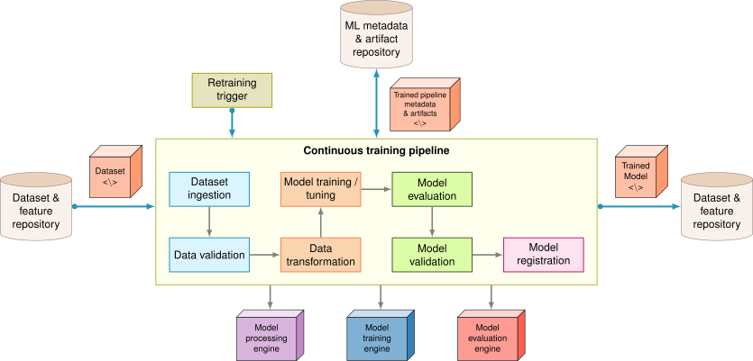](https://mlsysbook.ai/contents/core/ops/fd85dcf9abff1bb9fcca83cba14c933c9b79030c.svg "Figure 6: ML CI/CD Pipeline: Automated workflows streamline model development by integrating version control, testing, and deployment, enabling continuous delivery of updated models to production. This pipeline emphasizes data and model validation, automated retraining triggers, and model registration with metadata for reproducibility and governance. Source: HarvardX.")
Figure 6: **ML CI/CD Pipeline**: Automated workflows streamline model development by integrating version control, testing, and deployment, enabling continuous delivery of updated models to production. This pipeline emphasizes data and model validation, automated retraining triggers, and model registration with metadata for reproducibility and governance. Source: HarvardX.
To illustrate these concepts in practice, consider an image classification model under active development. When a data scientist commits changes to a [GitHub](https://github.com/)
repository, a Jenkins pipeline is triggered. The pipeline fetches the latest data, performs preprocessing, and initiates model training. Experiments are tracked using [MLflow](https://mlflow.org/)
, which logs metrics and stores model artifacts. After passing automated evaluation tests, the model is containerized and deployed to a staging environment using [Kubernetes](https://kubernetes.io/)
. If the model meets validation criteria in staging, the pipeline orchestrates controlled deployment strategies such as canary testing (detailed in [Section 1.4.2.3](https://mlsysbook.ai/contents/core/ops/ops.html#sec-ml-operations-model-validation-cb32)
), gradually routing production traffic to the new model while monitoring key metrics for anomalies. In case of performance regressions, the system can automatically revert to a previous model version.
Through these comprehensive automation capabilities, CI/CD pipelines play a central role in enabling scalable, repeatable, and safe deployment of machine learning models. By unifying the disparate stages of the ML workflow under continuous automation, these pipelines support faster iteration, improved reproducibility, and greater resilience in production systems. In mature MLOps environments, CI/CD is not an optional layer, but a foundational capability that transforms ad hoc experimentation into a structured and operationally sound development process.
#### Training Pipelines
Model training is a central phase in the machine learning lifecycle, where algorithms are optimized to learn patterns from data. Building on the distributed training concepts covered in **[Chapter 8: AI Training](https://mlsysbook.ai/contents/core/training/training.html#sec-ai-training)
**, we examine how training workflows are operationalized through systematic pipelines. Within an MLOps context, these activities are reframed as part of a reproducible, scalable, and automated pipeline that supports continual experimentation and reliable production deployment.
The foundation of operational training lies in modern machine learning frameworks such as [TensorFlow](https://www.tensorflow.org/)
, [PyTorch](https://pytorch.org/)
, and [Keras](https://keras.io/)
, which provide modular components for building and training models. The framework selection principles from **[Chapter 7: AI Frameworks](https://mlsysbook.ai/contents/core/frameworks/frameworks.html#sec-ai-frameworks)
** become essential for production training pipelines requiring reliable scaling. These libraries include high-level abstractions for neural network components and training algorithms, enabling practitioners to prototype and iterate efficiently. When embedded into MLOps pipelines, these frameworks serve as the foundation for training processes that can be systematically scaled, tracked, and retrained.
Building on these framework foundations, reproducibility emerges as a key objective of MLOps. Training scripts and configurations are version-controlled using tools like [Git](https://git-scm.com/)
and hosted on platforms such as [GitHub](https://github.com/)
. Interactive development environments, including [Jupyter](https://jupyter.org/)
notebooks, encapsulate data ingestion, feature engineering, training routines, and evaluation logic in a unified format. These notebooks integrate into automated pipelines, allowing the same logic used for local experimentation to be reused for scheduled retraining in production systems.
Beyond ensuring reproducibility, automation further enhances model training by reducing manual effort and standardizing critical steps. MLOps workflows incorporate techniques such as [hyperparameter tuning](https://cloud.google.com/ai-platform/training/docs/hyperparameter-tuning-overview)
, [neural architecture search](https://arxiv.org/abs/1808.05377)
, and [automatic feature selection](https://scikit-learn.org/stable/modules/feature_selection.html)
to explore the design space efficiently. These tasks are orchestrated using CI/CD pipelines, which automate data preprocessing, model training, evaluation, registration, and deployment. For instance, a Jenkins pipeline triggers a retraining job when new labeled data becomes available. The resulting model is evaluated against baseline metrics, and if performance thresholds are met, it is deployed automatically.
Supporting these automated workflows, the increasing availability of cloud-based infrastructure has further expanded the reach of model training. This connects to the workflow orchestration patterns explored in **[Chapter 5: AI Workflow](https://mlsysbook.ai/contents/core/workflow/workflow.html#sec-ai-workflow)
**, which provide the foundation for managing complex, multi-stage training processes across distributed systems. Cloud providers offer managed services that provision high-performance computing resources, which include GPU and TPU accelerators, on demand[19](https://mlsysbook.ai/contents/core/ops/ops.html#fn19)
. Depending on the platform, teams construct their own training workflows or rely on fully managed services such as [Vertex AI Fine Tuning](https://cloud.google.com/vertex-ai/docs/generative-ai/models/tune-models)
, which support automated adaptation of foundation models to new tasks. Nonetheless, hardware availability, regional access restrictions, and cost constraints remain important considerations when designing cloud-based training systems.
19 **Cloud ML Training Economics**: Training GPT-3 was estimated to cost approximately $4.6 million on AWS according to Lambda Labs calculations, though official training costs were not disclosed by OpenAI, while fine-tuning typically costs $100-$10,000. Google’s TPU v4 pods can reduce training costs by 2-5\\(\\times\\) compared to equivalent GPU clusters, with some organizations reporting 60-80% cost savings through spot instances and preemptible training.
To illustrate these integrated practices, consider a data scientist developing a neural network for image classification using a PyTorch notebook. The [fastai](https://www.fast.ai/)
library is used to simplify model construction and training. The notebook trains the model on a labeled dataset, computes performance metrics, and tunes model configuration parameters. Once validated, the training script is version-controlled and incorporated into a retraining pipeline that is periodically triggered based on data updates or model performance monitoring.
Through standardized workflows, versioned environments, and automated orchestration, MLOps enables the model training process to transition from ad hoc experimentation to a robust, repeatable, and scalable system. This not only accelerates development but also ensures that trained models meet production standards for reliability, traceability, and performance.
#### Model Validation
Before a machine learning model is deployed into production, it must undergo rigorous evaluation to ensure that it meets predefined performance, robustness, and reliability criteria. While earlier chapters discussed evaluation in the context of model development, MLOps reframes evaluation as a structured and repeatable process for validating operational readiness. It incorporates practices that support pre-deployment assessment, post-deployment monitoring, and automated regression testing.
The evaluation process begins with performance testing against a holdout test set, a dataset not used during training or validation. This dataset is sampled from the same distribution as production data and is used to measure generalization. Core metrics such as [accuracy](https://en.wikipedia.org/wiki/Accuracy_and_precision)
, [area under the curve (AUC)](https://en.wikipedia.org/wiki/Receiver_operating_characteristic#Area_under_the_curve)
, [precision](https://en.wikipedia.org/wiki/Precision_and_recall)
, [recall](https://en.wikipedia.org/wiki/Precision_and_recall)
, and [F1 score](https://en.wikipedia.org/wiki/F1_score)
are computed to quantify model performance. These metrics are not only used at a single point in time but also tracked longitudinally to detect degradation, such as that caused by [data drift](https://www.ibm.com/cloud/learn/data-drift)
, where shifts in input distributions can reduce model accuracy over time (see [Figure 7](https://mlsysbook.ai/contents/core/ops/ops.html#fig-data-drift)
).
[](https://mlsysbook.ai/contents/core/ops/62f4823c49384eecdfb435aec469e761771b64fd.svg "Figure 7: Data Drift Impact: Declining model performance over time results from data drift, where the characteristics of production data diverge from the training dataset. Monitoring key metrics longitudinally allows MLOps engineers to detect this drift and trigger model retraining or data pipeline adjustments to maintain accuracy.")
Figure 7: **Data Drift Impact**: Declining model performance over time results from data drift, where the characteristics of production data diverge from the training dataset. Monitoring key metrics longitudinally allows MLOps engineers to detect this drift and trigger model retraining or data pipeline adjustments to maintain accuracy.
Beyond static evaluation, MLOps encourages controlled deployment strategies that simulate production conditions while minimizing risk. One widely adopted method is [canary testing](https://martinfowler.com/bliki/CanaryRelease.html)
, in which the new model is deployed to a small fraction of users or queries. During this limited rollout, live performance metrics are monitored to assess system stability and user impact. For instance, an e-commerce platform deploys a new recommendation model to 5% of web traffic and observes metrics such as click-through rate, latency, and prediction accuracy. Only after the model demonstrates consistent and reliable performance is it promoted to full production.
Cloud-based ML platforms further support model evaluation by enabling experiment logging, request replay, and synthetic test case generation. These capabilities allow teams to evaluate different models under identical conditions, facilitating comparisons and root-cause analysis. Tools such as [Weights and Biases](https://wandb.ai/)
automate aspects of this process by capturing training artifacts, recording hyperparameter configurations, and visualizing performance metrics across experiments. These tools integrate directly into training and deployment pipelines, improving transparency and traceability.
While automation is central to MLOps evaluation practices, human oversight remains essential. Automated tests may fail to capture nuanced performance issues, such as poor generalization on rare subpopulations or shifts in user behavior. Therefore, teams combine quantitative evaluation with qualitative review, particularly for models deployed in high-stakes or regulated environments. This human-in-the-loop validation becomes especially critical for social impact applications, where model failures can have direct consequences on vulnerable populations.
This multi-stage evaluation process bridges offline testing and live system monitoring, ensuring that models not only meet technical benchmarks but also behave predictably and responsibly under real-world conditions. These evaluation practices reduce deployment risk and help maintain the reliability of machine learning systems over time, completing the development infrastructure foundation necessary for production deployment.
### Infrastructure Integration Summary
The infrastructure and development components examined in this section establish the foundation for reliable machine learning operations. These systems transform ad hoc experimentation into structured workflows that support reproducibility, collaboration, and continuous improvement.
**Data infrastructure** provides the foundation through feature stores that enable feature reuse across projects, versioning systems that track data lineage and evolution, and validation frameworks that ensure data quality throughout the pipeline. Building on the data management foundations from **[Chapter 6: Data Engineering](https://mlsysbook.ai/contents/core/data_engineering/data_engineering.html#sec-data-engineering)
**, these components extend basic capabilities to production contexts where multiple teams and models depend on shared data assets.
**Continuous pipelines** automate the ML lifecycle through CI/CD systems adapted for machine learning workflows. Unlike traditional software CI/CD that focuses solely on code, ML pipelines orchestrate data validation, feature transformation, model training, and evaluation in integrated workflows. Training pipelines specifically manage the computationally intensive process of model development, coordinating resource allocation, hyperparameter optimization, and experiment tracking. These automated workflows enable teams to iterate rapidly while maintaining reproducibility and quality standards.
**Model validation** bridges development and production through systematic evaluation that extends beyond offline metrics. Validation strategies combine performance benchmarking on held-out datasets with canary testing in production environments, allowing teams to detect issues before full deployment. This multi-stage validation recognizes that models must perform not just on static test sets but under dynamic real-world conditions where data distributions shift and user behavior evolves.
These infrastructure components directly address the operational challenges identified earlier through systematic engineering capabilities:
* Feature stores and data versioning solve data dependency debt by ensuring consistent, tracked feature access across training and serving
* CI/CD pipelines and model registries prevent correction cascades through controlled deployment and rollback mechanisms
* Automated workflows and lineage tracking eliminate undeclared consumer risks via explicit dependency management
* Modular pipeline architectures avoid pipeline debt through reusable, well-defined component interfaces
However, deploying a validated model represents only the beginning of the production journey. The infrastructure enables reliable model development, but production operations must address the dynamic challenges of maintaining system performance under real-world conditions: handling data drift, managing system failures, and adapting to evolving requirements without service disruption.
**Self-Check: Question 1.4**
1. Which of the following best describes the role of feature stores in MLOps infrastructure?
1. They store raw data for model training.
2. They serve as repositories for model versioning.
3. They provide cloud storage solutions for data artifacts.
4. They manage engineered features for consistent access across training and inference.
2. How does the integration of CI/CD pipelines enhance the reliability and reproducibility of machine learning models in production?
3. Order the following MLOps infrastructure components from data ingestion to model deployment: (1) Data Management, (2) Model Training, (3) Feature Store, (4) Model Serving.
4. True or False: In MLOps, the primary purpose of data versioning is to ensure that model training can be reproduced exactly at any point in the future.
5. Consider a scenario where an industrial predictive maintenance system is deployed. What role does a feature store play in ensuring the system’s operational efficiency?
[See Answers →](https://mlsysbook.ai/contents/core/ops/ops.html#quiz-answer-sec-ml-operations-development-infrastructure-automation-0be4)
Production Operations
---------------------
Building directly on the infrastructure foundation established above, production operations transform validated models into reliable services that maintain performance under real-world conditions. These operations must handle the diverse requirements established in preceding chapters: managing model updates across distributed edge devices without centralized visibility (**[Chapter 14: On-Device Learning](https://mlsysbook.ai/contents/core/ondevice_learning/ondevice_learning.html#sec-ondevice-learning)
**), maintaining security controls during runtime inference and model updates (**[Chapter 15: Security & Privacy](https://mlsysbook.ai/contents/core/privacy_security/privacy_security.html#sec-security-privacy)
**), and detecting performance degradation from adversarial attacks or distribution shifts (**[Chapter 16: Robust AI](https://mlsysbook.ai/contents/core/robust_ai/robust_ai.html#sec-robust-ai)
**). This operational layer implements monitoring, governance, and deployment strategies that enable these specialized capabilities to function together reliably at scale.
This section explores the deployment patterns, serving infrastructure, monitoring systems, and governance frameworks that transform validated models into production services capable of operating reliably at scale.
Production operations introduce challenges that extend beyond model development. Deployed systems must handle variable loads, maintain consistent latency under diverse conditions, recover gracefully from failures, and adapt to evolving data distributions without disrupting service. These requirements demand specialized infrastructure, monitoring capabilities, and operational practices that complement the development workflows established in the previous section.
### Model Deployment and Serving
Once a model has been trained and validated, it must be integrated into a production environment where it can deliver predictions at scale. This process involves packaging the model with its dependencies, managing versions, and deploying it in a way that aligns with performance, reliability, and governance requirements. Deployment transforms a static artifact into a live system component. Serving ensures that the model is accessible, reliable, and efficient in responding to inference requests. Together, these components bridge model development and real-world impact.
#### Model Deployment
Teams need to properly package, test, and track ML models to reliably deploy them to production. MLOps introduces frameworks and procedures for actively versioning, deploying, monitoring, and updating models in sustainable ways.
One common approach to deployment involves containerizing models using containerization technologies[20](https://mlsysbook.ai/contents/core/ops/ops.html#fn20)
. This packaging approach ensures smooth portability across environments, making deployment consistent and predictable.
20 **Containerization and Orchestration**: Docker containers package applications with all their dependencies into standardized, portable units that run consistently across different computing environments, isolating software from infrastructure variations. Kubernetes orchestrates these containers at scale, automating deployment, load balancing, scaling, and recovery across clusters of machines. Together, they enable the reproducible, automated infrastructure management essential for modern MLOps, where models and their serving environments must be deployed consistently across development, staging, and production.
Production deployment requires frameworks that handle model packaging, versioning, and integration with serving infrastructure. Tools like MLflow and model registries manage these deployment artifacts, while serving-specific frameworks (detailed in the Inference Serving section) handle the runtime optimization and scaling requirements.
Before full-scale rollout, teams deploy updated models to staging or QA environments[21](https://mlsysbook.ai/contents/core/ops/ops.html#fn21)
to rigorously test performance.
21 **TensorFlow Serving Origins**: Born from Google’s internal serving system that handled billions of predictions per day for products like Gmail spam detection and YouTube recommendations. Google open-sourced it in 2016 when they realized that productionizing ML models was the bottleneck preventing widespread AI adoption.
22 **Canary Deployment History**: Named after the canaries miners used to detect toxic gases; if the bird died, miners knew to evacuate immediately. Netflix pioneered this technique for software in 2011, and it became essential for ML where model failures can be subtle and catastrophic.
23 **Blue-Green Deployment**: Zero-downtime deployment strategy maintaining two identical production environments. One serves traffic (blue) while the other receives updates (green). After validation, traffic switches instantly to green. For ML systems, this enables risk-free model updates since rollback takes <10 seconds vs. hours for model retraining. Spotify uses blue-green deployment for their recommendation models, serving 400+ million users with 99.95% uptime during model updates.
Techniques such as shadow deployments, canary testing[22](https://mlsysbook.ai/contents/core/ops/ops.html#fn22)
, and blue-green deployment[23](https://mlsysbook.ai/contents/core/ops/ops.html#fn23)
are used to validate new models incrementally. As described in our evaluation frameworks, these controlled deployment strategies enable safe model validation in production. Robust rollback procedures are essential to handle unexpected issues, reverting systems to the previous stable model version to ensure minimal disruption.
When canary deployments reveal problems at partial traffic levels (e.g., issues appearing at 30% traffic but not at 5%), teams need systematic debugging strategies. Effective diagnosis requires correlating multiple signals: performance metrics from **[Chapter 12: Benchmarking AI](https://mlsysbook.ai/contents/core/benchmarking/benchmarking.html#sec-benchmarking-ai)
**, data distribution analysis to detect drift, and feature importance shifts that might explain degradation. Teams maintain debug toolkits including A/B test[24](https://mlsysbook.ai/contents/core/ops/ops.html#fn24)
analysis frameworks, feature attribution tools, and data slice analyzers that identify which subpopulations are experiencing degraded performance.
24 **A/B Testing for ML**: Statistical method to compare model performance by splitting traffic between model versions. Netflix runs 1,000+ A/B tests annually on recommendation algorithms, while Uber tests ride pricing models on millions of trips daily to optimize both user experience and revenue. Rollback decisions must balance the severity of degradation against business impact: a 2% accuracy drop might be acceptable during feature launches but unacceptable for safety-critical applications.
Integration with CI/CD pipelines further automates the deployment and rollback process, enabling efficient iteration cycles.
Model registries, such as [Vertex AI’s model registry](https://cloud.google.com/vertex-ai/docs/model-registry/introduction)
, act as centralized repositories for storing and managing trained models. These registries not only facilitate version comparisons but also often include access to base models, which may be open source, proprietary, or a hybrid (e.g., [LLAMA](https://ai.meta.com/llama/)
). Deploying a model from the registry to an inference endpoint is streamlined, handling resource provisioning, model weight downloads, and hosting.
Inference endpoints typically expose the deployed model via REST APIs for real-time predictions. Depending on performance requirements, teams can configure resources, such as GPU accelerators, to meet latency and throughput targets. Some providers also offer flexible options like serverless[25](https://mlsysbook.ai/contents/core/ops/ops.html#fn25)
or batch inference, eliminating the need for persistent endpoints and enabling cost-efficient, scalable deployments.
25 **Serverless Computing for ML**: Infrastructure that automatically scales from zero to thousands of instances based on demand, with sub-second cold start times. AWS Lambda can handle 10,000+ concurrent ML inference requests, while Google Cloud Functions supports models up to 32 GB, charging only for actual compute time used. For example, [AWS SageMaker Inference](https://docs.aws.amazon.com/sagemaker/latest/dg/deploy-model.html)
supports such configurations.
26 **MLflow’s Creation**: Built by the team at Databricks who were frustrated watching their customers struggle with ML experiment tracking. They noticed that data scientists were keeping model results in spreadsheets and could never reproduce their best experiments, a problem that inspired MLflow’s “model registry” concept.
To maintain lineage and auditability, teams track model artifacts, including scripts, weights, logs, and metrics, using tools like [MLflow](https://mlflow.org/)
[26](https://mlsysbook.ai/contents/core/ops/ops.html#fn26)
.
By leveraging these tools and practices, teams can deploy ML models resiliently, ensuring smooth transitions between versions, maintaining production stability, and optimizing performance across diverse use cases.
#### Inference Serving
Once a model has been deployed, the final stage in operationalizing machine learning is to make it accessible to downstream applications or end-users. Serving infrastructure provides the interface between trained models and real-world systems, enabling predictions to be delivered reliably and efficiently. In large-scale settings, such as social media platforms or e-commerce services, serving systems may process tens of trillions of inference queries per day ([Wu et al. 2019](https://mlsysbook.ai/contents/core/ops/ops.html#ref-wu2019machine)
). The measurement frameworks established in **[Chapter 12: Benchmarking AI](https://mlsysbook.ai/contents/core/benchmarking/benchmarking.html#sec-benchmarking-ai)
** become essential for validating performance claims and establishing production baselines. Meeting such demand requires careful design to balance latency, scalability, and robustness.
Wu, Carole-Jean, David Brooks, Kevin Chen, Douglas Chen, Sy Choudhury, Marat Dukhan, Kim Hazelwood, et al. 2019. “Machine Learning at Facebook: Understanding Inference at the Edge.” In _2019 IEEE International Symposium on High Performance Computer Architecture (HPCA)_, 331–44. IEEE; IEEE. [https://doi.org/10.1109/hpca.2019.00048](https://doi.org/10.1109/hpca.2019.00048)
.
27 **TensorFlow Serving**: Google’s production-grade ML serving system handles over 100,000 queries per second per machine for lightweight models on high-end hardware with <10 ms latency for most models. Originally built to serve YouTube’s recommendation system, processing over 1 billion hours of video watched daily.
28 **NVIDIA Triton Inference Server**: Can achieve up to 40,000 inferences per second on a single A100 GPU for BERT models, with dynamic batching reducing latency by up to 10\\(\\times\\) compared to naive serving approaches. Supports concurrent execution of up to 100 different model types.
29 **KServe (formerly KFServing)**: Kubernetes-native serving framework that can autoscale from zero to thousands of replicas in under 30 seconds. Used by companies like Bloomberg to serve over 10,000 models simultaneously with 99.9% uptime SLA.
To address these challenges, production-grade serving frameworks have emerged. Tools such as [TensorFlow Serving](https://www.tensorflow.org/tfx/guide/serving)
[27](https://mlsysbook.ai/contents/core/ops/ops.html#fn27)
, [NVIDIA Triton Inference Server](https://developer.nvidia.com/triton-inference-server)
[28](https://mlsysbook.ai/contents/core/ops/ops.html#fn28)
, and [KServe](https://kserve.github.io/website/latest/)
[29](https://mlsysbook.ai/contents/core/ops/ops.html#fn29)
provide standardized mechanisms for deploying, versioning, and scaling machine learning models across heterogeneous infrastructure. These frameworks abstract many of the lower-level concerns, allowing teams to focus on system behavior, integration, and performance targets.
Model serving architectures are typically designed around three broad paradigms:
1. Online Serving, which provides low-latency, real-time predictions for interactive systems such as recommendation engines or fraud detection.
2. Offline Serving, which processes large batches of data asynchronously, typically in scheduled jobs used for reporting or model retraining.
3. Near-Online (Semi-Synchronous) Serving, which offers a balance between latency and throughput, appropriate for scenarios like chatbots or semi-interactive analytics.
Each of these approaches introduces different constraints in terms of availability, responsiveness, and throughput. The efficiency techniques from **[Chapter 9: Efficient AI](https://mlsysbook.ai/contents/core/efficient_ai/efficient_ai.html#sec-efficient-ai)
** become crucial for meeting these performance requirements, particularly when serving models at scale. Serving systems are therefore constructed to meet specific Service Level Agreements (SLAs)[30](https://mlsysbook.ai/contents/core/ops/ops.html#fn30)
and Service Level Objectives (SLOs)[31](https://mlsysbook.ai/contents/core/ops/ops.html#fn31)
, which quantify acceptable performance boundaries along dimensions such as latency, error rates, and uptime. Achieving these goals requires a range of optimizations in request handling, scheduling, and resource allocation.
30 **Service Level Agreements (SLAs)**: Production ML systems typically target 99.9% uptime (8.77 hours downtime/year) for critical services, with penalties of 10-25% monthly service credits for each 0.1% below target. Google’s Cloud AI Platform promises 99.95% uptime with automatic failover in <30 seconds.
31 **Service Level Objectives (SLOs)**: Real-world ML serving SLOs often specify P95 latency <100 ms for online inference, P99 <500 ms, and error rates <0.1%. Netflix’s recommendation system maintains P99 latency under 150 ms while serving 200+ million users, processing 3+ billion hours of content monthly.
A number of serving system design strategies are commonly employed to meet these requirements. Request scheduling and batching aggregate inference requests to improve throughput and hardware utilization. For instance, Clipper ([Crankshaw et al. 2017](https://mlsysbook.ai/contents/core/ops/ops.html#ref-crankshaw2017clipper)
) applies batching and caching to reduce response times in online settings. Model instance selection and routing dynamically assign requests to model variants based on system load or user-defined constraints; INFaaS ([Romero et al. 2021](https://mlsysbook.ai/contents/core/ops/ops.html#ref-romero2021infaas)
) illustrates this approach by optimizing accuracy-latency trade-offs across variant models.
1. **Request scheduling and batching**: Efficiently manages incoming ML inference requests, optimizing performance through smart queuing and grouping strategies. Systems like Clipper ([Crankshaw et al. 2017](https://mlsysbook.ai/contents/core/ops/ops.html#ref-crankshaw2017clipper)
) introduce low-latency online prediction serving with caching and batching techniques.
2. **Model instance selection and routing**: Intelligent algorithms direct requests to appropriate model versions or instances. INFaaS ([Romero et al. 2021](https://mlsysbook.ai/contents/core/ops/ops.html#ref-romero2021infaas)
) explores this by generating model-variants and efficiently exploring the trade-off space based on performance and accuracy requirements.
3. **Load balancing**: Distributes workloads evenly across multiple serving instances. MArk (Model Ark) ([C. Zhang et al. 2019](https://mlsysbook.ai/contents/core/ops/ops.html#ref-zhang2019mark)
) demonstrates effective load balancing techniques for ML serving systems.
4. **Model instance autoscaling**: Dynamically adjusts capacity based on demand. Both INFaaS ([Romero et al. 2021](https://mlsysbook.ai/contents/core/ops/ops.html#ref-romero2021infaas)
) and MArk ([C. Zhang et al. 2019](https://mlsysbook.ai/contents/core/ops/ops.html#ref-zhang2019mark)
) incorporate autoscaling capabilities to handle workload fluctuations efficiently.
5. **Model orchestration**: Manages model execution, enabling parallel processing and strategic resource allocation. AlpaServe ([Li et al. 2023](https://mlsysbook.ai/contents/core/ops/ops.html#ref-li2023alpaserve)
) demonstrates advanced techniques for handling large models and complex serving scenarios.
6. **Execution time prediction**: Systems like Clockwork ([Gujarati et al. 2020](https://mlsysbook.ai/contents/core/ops/ops.html#ref-gujarati2020serving)
) focus on high-performance serving by predicting execution times of individual inferences and efficiently using hardware accelerators.
Crankshaw, Daniel, Xin Wang, Guilio Zhou, Michael J Franklin, Joseph E Gonzalez, and Ion Stoica. 2017. “Clipper: A \\(\\{\\)Low-Latency\\(\\}\\) Online Prediction Serving System.” In _14th USENIX Symposium on Networked Systems Design and Implementation (NSDI 17)_, 613–27.
Romero, Francisco, Qian Li 0027, Neeraja J. Yadwadkar, and Christos Kozyrakis. 2021. “INFaaS: Automated Model-Less Inference Serving.” In _2021 USENIX Annual Technical Conference (USENIX ATC 21)_, 397–411. [https://www.usenix.org/conference/atc21/presentation/romero](https://www.usenix.org/conference/atc21/presentation/romero)
.
Zhang, Chengliang, Minchen Yu, Wei Wang 0030, and Feng Yan 0001. 2019. “MArk: Exploiting Cloud Services for Cost-Effective, SLO-Aware Machine Learning Inference Serving.” In _2019 USENIX Annual Technical Conference (USENIX ATC 19)_, 1049–62. [https://www.usenix.org/conference/atc19/presentation/zhang-chengliang](https://www.usenix.org/conference/atc19/presentation/zhang-chengliang)
.
Li, Zhuohan, Lianmin Zheng, Yinmin Zhong, Vincent Liu, Ying Sheng, Xin Jin, Yanping Huang, et al. 2023. “\\(\\{\\)AlpaServe\\(\\}\\): Statistical Multiplexing with Model Parallelism for Deep Learning Serving.” In _17th USENIX Symposium on Operating Systems Design and Implementation (OSDI 23)_, 663–79.
Gujarati, Arpan, Reza Karimi, Safya Alzayat, Wei Hao, Antoine Kaufmann, Ymir Vigfusson, and Jonathan Mace. 2020. “Serving DNNs Like Clockwork: Performance Predictability from the Bottom Up.” In _14th USENIX Symposium on Operating Systems Design and Implementation (OSDI 20)_, 443–62. [https://www.usenix.org/conference/osdi20/presentation/gujarati](https://www.usenix.org/conference/osdi20/presentation/gujarati)
.
In more complex inference scenarios, model orchestration coordinates the execution of multi-stage models or distributed components. AlpaServe ([Li et al. 2023](https://mlsysbook.ai/contents/core/ops/ops.html#ref-li2023alpaserve)
) exemplifies this by enabling efficient serving of large foundation models through coordinated resource allocation. Finally, execution time prediction enables systems to anticipate latency for individual requests. Clockwork ([Gujarati et al. 2020](https://mlsysbook.ai/contents/core/ops/ops.html#ref-gujarati2020serving)
) uses this capability to reduce tail latency and improve scheduling efficiency under high load.
While these systems differ in implementation, they collectively illustrate the critical techniques that underpin scalable and responsive ML-as-a-Service infrastructure. [Table 2](https://mlsysbook.ai/contents/core/ops/ops.html#tbl-serving-techniques)
summarizes these strategies and highlights representative systems that implement them.
Table 2: **Serving System Techniques**: Scalable ML-as-a-service infrastructure relies on techniques like request scheduling and instance selection to optimize resource utilization and reduce latency under high load. The table summarizes key strategies and representative systems (clipper, for example) that implement them for efficient deployment of machine learning models.
| | | |
| --- | --- | --- |
| **Request Scheduling & Batching** | Groups inference requests to improve throughput and reduce overhead | Clipper |
| **Instance Selection & Routing** | Dynamically assigns requests to model variants based on constraints | INFaaS |
| **Load Balancing** | Distributes traffic across replicas to prevent bottlenecks | MArk |
| **Autoscaling** | Adjusts model instances to match workload demands | INFaaS, MArk |
| **Model Orchestration** | Coordinates execution across model components or pipelines | AlpaServe |
| **Execution Time Prediction** | Forecasts latency to optimize request scheduling | Clockwork |
Together, these strategies form the foundation of robust model serving systems. When effectively integrated, they enable machine learning applications to meet performance targets while maintaining system-level efficiency and scalability.
#### Edge AI Deployment Patterns
Edge AI represents a major shift in deployment architecture where machine learning inference occurs at or near the data source, rather than in centralized cloud infrastructure. This paradigm addresses critical constraints including latency requirements, bandwidth limitations, privacy concerns, and connectivity constraints that characterize real-world operational environments. According to industry projections, 75% of ML inference will occur at the edge by 2025, making edge deployment patterns essential knowledge for MLOps practitioners ([Reddi et al. 2019](https://mlsysbook.ai/contents/core/ops/ops.html#ref-reddi2023mlperf)
).
Reddi, Vijay Janapa, Christine Cheng, David Kanter, Peter Mattson, Guenther Schmuelling, Carole-Jean Wu, Brian Anderson, et al. 2019. “MLPerf Inference Benchmark.” _arXiv Preprint arXiv:1911.02549_, November. [http://arxiv.org/abs/1911.02549v2](http://arxiv.org/abs/1911.02549v2)
.
Edge deployment introduces unique operational challenges that distinguish it from traditional cloud-centric MLOps. Resource constraints on edge devices require aggressive model optimization techniques including quantization, pruning, and knowledge distillation to achieve sub-1 MB memory footprints while maintaining acceptable accuracy. Power budgets for edge devices typically range from 10 mW for IoT sensors to 45 W for automotive systems, demanding power-aware inference scheduling and thermal management strategies. Real-time requirements for safety-critical applications necessitate deterministic inference timing with worst-case execution time guarantees under 10 ms for collision avoidance systems and sub-100 ms for interactive robotics applications.
The operational architecture for edge AI systems typically follows hierarchical deployment patterns that distribute intelligence across multiple tiers. Sensor-level processing handles immediate data filtering and feature extraction with microcontroller-class devices consuming 1-100 mW. Edge gateway processing performs intermediate inference tasks using application processors with 1-10 W power budgets. Cloud coordination manages model distribution, aggregated learning, and complex reasoning tasks requiring GPU-class computational resources. This hierarchy enables system-wide optimization where computationally expensive operations migrate to higher tiers while latency-critical decisions remain local.
The most resource-constrained edge AI scenarios involve TinyML deployment patterns, targeting microcontroller-based inference with memory constraints under 1 MB and power consumption measured in milliwatts. TinyML deployment requires specialized inference engines such as TensorFlow Lite Micro, CMSIS-NN, and hardware-specific optimized libraries that eliminate dynamic memory allocation and minimize computational overhead. Model architectures must be co-designed with hardware constraints, favoring depthwise convolutions, binary neural networks, and pruned models that achieve 90%+ sparsity while maintaining task-specific accuracy requirements.
Mobile AI operations extend this edge deployment paradigm to smartphones and tablets with moderate computational capabilities and strict power efficiency requirements. Mobile deployment leverages hardware acceleration through Neural Processing Units (NPUs), GPU compute shaders, and specialized instruction sets to achieve inference performance targets of 5-50 ms latency with power consumption under 500 mW. Mobile AI operations require sophisticated power management including dynamic frequency scaling, thermal throttling coordination, and background inference scheduling that balances performance against battery life and user experience constraints.
Critical operational capabilities for deployed edge systems include over-the-air model updates, which enable maintenance for systems that cannot be physically accessed. OTA update pipelines must implement secure, verified model distribution that prevents malicious model injection while ensuring update integrity through cryptographic signatures and rollback mechanisms. Edge devices require differential compression techniques that minimize bandwidth usage by transmitting only model parameter changes rather than complete model artifacts. Update scheduling must account for device connectivity patterns, power availability, and operational criticality to prevent update-induced service disruptions.
Production edge AI systems implement real-time constraint management through systematic approaches to deadline analysis and resource allocation. Worst-case execution time (WCET) analysis ensures that inference operations complete within specified timing bounds even under adverse conditions including thermal throttling, memory contention, and interrupt service routines. Resource reservation mechanisms guarantee computational bandwidth for safety-critical inference tasks while enabling best-effort execution of non-critical workloads. Graceful degradation strategies enable systems to maintain essential functionality when resources become constrained by reducing model complexity, inference frequency, or feature completeness.
Edge-cloud coordination patterns enable hybrid deployment architectures that optimize the distribution of inference workloads across computational tiers. Adaptive offloading strategies dynamically route inference requests between edge and cloud resources based on current system load, network conditions, and latency requirements. Feature caching at edge gateways reduces redundant computation by storing frequently accessed intermediate representations while maintaining data freshness through cache invalidation policies. Federated learning coordination enables edge devices to contribute to model improvement without transmitting raw data, addressing privacy constraints while maintaining system-wide learning capabilities.
The operational complexity of edge AI deployment requires specialized monitoring and debugging approaches adapted to resource-constrained environments. Lightweight telemetry systems capture essential performance metrics including inference latency, power consumption, and accuracy indicators while minimizing overhead on edge devices. Remote debugging capabilities enable engineers to diagnose deployed systems through secure channels that preserve privacy while providing sufficient visibility into system behavior. Health monitoring systems track device-level conditions including thermal status, battery levels, and connectivity quality to predict maintenance requirements and prevent catastrophic failures.
Resource constraint analysis underpins successful edge AI deployment by systematically modeling the trade-offs between computational capability, power consumption, memory utilization, and inference accuracy. Power budgeting frameworks establish operational envelopes that define sustainable workload configurations under varying environmental conditions and usage patterns. Memory optimization hierarchies guide the selection of model compression techniques, from parameter reduction through structural simplification to architectural modifications that reduce computational requirements.
Edge AI deployment represents the operational frontier where MLOps practices must adapt to the physical constraints and distributed complexity of real-world systems. Success requires not only technical expertise in model optimization and embedded systems but also systematic approaches to distributed system management, security, and reliability engineering that ensure deployed systems remain functional across diverse operational environments.
### Resource Management and Performance Monitoring
The operational stability of a machine learning system depends on the robustness of its underlying infrastructure. Compute, storage, and networking resources must be provisioned, configured, and scaled to accommodate training workloads, deployment pipelines, and real-time inference. Beyond infrastructure provisioning, effective observability practices ensure that system behavior can be monitored, interpreted, and acted upon as conditions change.
#### Infrastructure Management
Scalable, resilient infrastructure is a foundational requirement for operationalizing machine learning systems. As models move from experimentation to production, MLOps teams must ensure that the underlying computational resources can support continuous integration, large-scale training, automated deployment, and real-time inference. This requires managing infrastructure not as static hardware, but as a dynamic, programmable, and versioned system.
To achieve this, teams adopt the practice of Infrastructure as Code (IaC), a paradigm that transforms how computing infrastructure is managed. Rather than manually configuring servers, networks, and storage through graphical interfaces or command-line tools, a process prone to human error and difficult to reproduce, IaC treats infrastructure configuration as software code. This code describes the desired state of infrastructure resources in text files that are version-controlled, reviewed, and automatically executed. Just as software developers write code to define application behavior, infrastructure engineers write code to define computing environments. This transformation brings software engineering best practices to infrastructure management: changes are tracked through version control, configurations can be tested before deployment, and entire environments can be reliably reproduced from their code definitions.
Tools such as [Terraform](https://www.terraform.io/)
, [AWS CloudFormation](https://aws.amazon.com/cloudformation/)
, and [Ansible](https://www.ansible.com/)
support this paradigm by enabling teams to version infrastructure definitions alongside application code. In MLOps settings, Terraform is widely used to provision and manage resources across public cloud platforms such as [AWS](https://aws.amazon.com/)
, [Google Cloud Platform](https://cloud.google.com/)
, and [Microsoft Azure](https://azure.microsoft.com/)
.
Infrastructure management spans the full lifecycle of ML systems. During model training, teams use IaC scripts to allocate compute instances with GPU or TPU accelerators, configure distributed storage, and deploy container clusters. These configurations ensure that data scientists and ML engineers access reproducible environments with the required computational capacity. Because infrastructure definitions are stored as code, they are audited, reused, and integrated into CI/CD pipelines to ensure consistency across environments.
Containerization plays a critical role in making ML workloads portable and consistent. Tools like [Docker](https://www.docker.com/)
encapsulate models and their dependencies into isolated units, while orchestration systems such as [Kubernetes](https://kubernetes.io/)
manage containerized workloads across clusters. These systems enable rapid deployment, resource allocation, and scaling, capabilities that are essential in production environments where workloads can vary dynamically.
To handle changes in workload intensity, including spikes during hyperparameter tuning and surges in prediction traffic, teams rely on cloud elasticity and autoscaling[32](https://mlsysbook.ai/contents/core/ops/ops.html#fn32)
. Cloud platforms support on-demand provisioning and horizontal scaling of infrastructure resources. [Autoscaling mechanisms](https://aws.amazon.com/autoscaling/)
automatically adjust compute capacity based on usage metrics, enabling teams to optimize for both performance and cost-efficiency.
32 **ML Autoscaling at Scale**: Kubernetes-based ML serving can scale from 1 to 1,000+ replicas in under 60 seconds. Uber’s ML platform automatically scales 2,000+ models daily, reducing infrastructure costs by 35-50% through intelligent resource allocation and cold-start optimization achieving 99.95% availability.
Infrastructure in MLOps is not limited to the cloud. Many deployments span on-premises, cloud, and edge environments, depending on latency, privacy, or regulatory constraints. A robust infrastructure management strategy must accommodate this diversity by offering flexible deployment targets and consistent configuration management across environments.
To illustrate, consider a scenario in which a team uses Terraform to deploy a Kubernetes cluster on Google Cloud Platform. The cluster is configured to host containerized TensorFlow models that serve predictions via HTTP APIs. As user demand increases, Kubernetes automatically scales the number of pods to handle the load. Meanwhile, CI/CD pipelines update the model containers based on retraining cycles, and monitoring tools track cluster performance, latency, and resource utilization. All infrastructure components, ranging from network configurations to compute quotas, are managed as version-controlled code, ensuring reproducibility and auditability.
By adopting Infrastructure as Code, leveraging cloud-native orchestration, and supporting automated scaling, MLOps teams gain the ability to provision and maintain the resources required for machine learning at production scale. This infrastructure layer underpins the entire MLOps stack, enabling reliable training, deployment, and serving workflows.
While these foundational capabilities address infrastructure provisioning and management, the operational reality of ML systems introduces unique resource optimization challenges that extend beyond traditional web service scaling patterns. Infrastructure resource management in MLOps becomes a multi-dimensional optimization problem, requiring teams to balance competing objectives: computational cost, model accuracy, inference latency, and training throughput.
ML workloads exhibit different resource consumption patterns compared to stateless web applications. Training workloads demonstrate bursty resource requirements, scaling from zero to thousands of GPUs during model development phases, then returning to minimal consumption during validation periods. This creates a tension between resource utilization efficiency and time-to-insight that traditional scaling approaches cannot adequately address. Conversely, inference workloads present steady resource consumption patterns with strict latency requirements that must be maintained under variable traffic patterns.
The optimization challenge intensifies when considering the interdependencies between training frequency, model complexity, and serving infrastructure costs. Effective resource management requires holistic approaches that model the entire system rather than optimizing individual components in isolation, taking into account factors such as data pipeline throughput, model retraining schedules, and serving capacity planning.
Hardware-aware resource optimization emerges as a critical operational discipline that bridges infrastructure efficiency with model performance. Production MLOps teams must establish utilization targets that balance cost efficiency against operational reliability: GPU utilization should consistently exceed 80% for batch training workloads to justify hardware costs, while serving workloads require sustained utilization above 60% to maintain economically viable inference operations. Memory bandwidth utilization patterns become equally important, as underutilized memory interfaces indicate suboptimal data pipeline configurations that can degrade training throughput by 30-50%.
Operational resource allocation extends beyond simple utilization metrics to encompass power budget management across mixed workloads. Production deployments typically allocate 60-70% of power budgets to training operations during development cycles, reserving 30-40% for sustained inference workloads. This allocation shifts dynamically based on business priorities: recommendation systems might reallocate power toward inference during peak traffic periods, while research environments prioritize training resource availability. Thermal management considerations become operational constraints rather than hardware design concerns, as sustained high-utilization workloads must be scheduled with cooling capacity limitations and thermal throttling thresholds that can impact SLA compliance.
#### Model and Infrastructure Monitoring
Monitoring is a critical function in MLOps, enabling teams to maintain operational visibility over machine learning systems deployed in production. Once a model is live, it becomes exposed to real-world inputs, evolving data distributions, and shifting user behavior. Without continuous monitoring, it becomes difficult to detect performance degradation, data quality issues, or system failures in a timely manner.
Effective monitoring spans both model behavior and infrastructure performance. On the model side, teams track metrics such as accuracy, precision, recall, and the [confusion matrix](https://scikit-learn.org/stable/auto_examples/model_selection/plot_confusion_matrix.html)
using live or sampled predictions. By evaluating these metrics over time, they can detect whether the model’s performance remains stable or begins to drift.
Production ML systems face model drift[33](https://mlsysbook.ai/contents/core/ops/ops.html#fn33)
(see [Section 1.4.2.3](https://mlsysbook.ai/contents/core/ops/ops.html#sec-ml-operations-model-validation-cb32)
for detailed analysis), which manifests in two main forms:
33 **Model Drift Detection**: Production systems typically trigger alerts when accuracy drops >5% over 24 hours or >10% over a week. Advanced systems like those at Spotify detect drift within 2-4 hours using statistical tests, with 85% of drift incidents caught before user impact.
* Concept drift[34](https://mlsysbook.ai/contents/core/ops/ops.html#fn34)
occurs when the underlying relationship between features and targets evolves. For example, during the COVID-19 pandemic, purchasing behavior shifted dramatically, invalidating many previously accurate recommendation models.
34 **COVID-19 ML Impact**: E-commerce recommendation systems saw accuracy drops of 15-40% within weeks of lockdowns beginning in March 2020. Amazon reported having to retrain over 1,000 models, while Netflix saw a 25% increase in viewing time that broke their capacity planning models.
* Data drift refers to shifts in the input data distribution itself. In applications such as self-driving cars, this may result from seasonal changes in weather, lighting, or road conditions, all of which affect the model’s inputs.
Beyond these recognized drift patterns lies a more insidious challenge: gradual long-term degradation that evades standard detection thresholds. Unlike sudden distribution shifts that trigger immediate alerts, some models experience performance erosion over months through imperceptible daily changes. For instance, e-commerce recommendation systems may lose 0.05% accuracy daily as user preferences evolve, accumulating to 15% degradation over a year without triggering monthly drift alerts. Seasonal patterns compound this complexity: a model trained in summer may perform well through autumn but fail catastrophically in winter conditions it never observed. Detecting such gradual degradation requires specialized monitoring approaches: establishing performance baselines across multiple time horizons (daily, weekly, quarterly), implementing sliding window comparisons that detect slow trends, and maintaining seasonal performance profiles that account for cyclical patterns. Teams often discover these degradations only through quarterly business reviews when cumulative impact becomes visible, emphasizing the need for multi-timescale monitoring strategies.
In addition to model-level monitoring, infrastructure-level monitoring tracks indicators such as CPU and GPU utilization, memory and disk consumption, network latency, and service availability. These signals help ensure that the system remains performant and responsive under varying load conditions. Hardware-aware monitoring extends these basic metrics to capture resource efficiency patterns critical for operational success: GPU memory bandwidth utilization, power consumption relative to computational output, and thermal envelope adherence across sustained workloads.
Building on the monitoring infrastructure outlined above, production systems must track hardware efficiency metrics that directly impact operational costs and model performance. GPU utilization monitoring should distinguish between compute-bound and memory-bound operations, as identical 90% utilization metrics can represent vastly different operational efficiency depending on bottleneck location. Memory bandwidth monitoring becomes essential for detecting suboptimal data loading patterns that manifest as high GPU utilization with low computational throughput. Power efficiency metrics, measured as operations per watt, enable teams to optimize mixed workload scheduling for both cost and environmental impact.
Thermal monitoring integrates into operational scheduling decisions, particularly for sustained high-utilization deployments where thermal throttling can degrade performance unpredictably. Modern MLOps monitoring dashboards incorporate thermal headroom metrics that guide workload distribution across available hardware, preventing thermal-induced performance degradation that can violate inference latency SLAs. Tools such as [Prometheus](https://prometheus.io/)
[35](https://mlsysbook.ai/contents/core/ops/ops.html#fn35)
, [Grafana](https://grafana.com/)
, and [Elastic](https://www.elastic.co/)
are widely used to collect, aggregate, and visualize these operational metrics. These tools often integrate into dashboards that offer real-time and historical views of system behavior.
35 **Prometheus at Scale**: Can ingest 1+ million samples per second per instance, with some deployments monitoring 100,000+ machines. DigitalOcean’s Prometheus setup stores 2+ years of metrics data across 40,000+ time series, with query response times under 100 ms for 95% of requests.
36 **Production Alert Thresholds**: Typical ML production alerts fire when GPU memory >90%, CPU >85% for >5 minutes, P99 latency \\(>2\\times\\) normal for >10 minutes, or error rates >1% for >60 seconds. Hardware-aware alerting extends these thresholds to include GPU utilization <60% for serving workloads (indicating resource waste), memory bandwidth utilization <40% (suggesting data pipeline bottlenecks), power consumption >110% of budget allocation (thermal risk), and thermal throttling events (immediate performance impact). High-frequency trading firms use microsecond-level alerts, while batch processing systems may use hour-long windows.
Proactive alerting mechanisms are configured to notify teams when anomalies or threshold violations occur[36](https://mlsysbook.ai/contents/core/ops/ops.html#fn36)
. For example, a sustained drop in model accuracy may trigger an alert to investigate potential drift, prompting retraining with updated data. Similarly, infrastructure alerts can signal memory saturation or degraded network performance, allowing engineers to take corrective action before failures propagate.
Ultimately, robust monitoring enables teams to detect problems before they escalate, maintain high service availability, and preserve the reliability and trustworthiness of machine learning systems. In the absence of such practices, models may silently degrade or systems may fail under load, undermining the effectiveness of the ML pipeline as a whole.
The monitoring systems themselves require resilience planning to prevent operational blind spots. When primary monitoring infrastructure fails, such as Prometheus experiencing downtime or Grafana becoming unavailable, teams risk operating blind during critical periods. Production-grade MLOps implementations therefore maintain redundant monitoring pathways: secondary metric collectors that activate during primary system failures, local logging that persists when centralized systems fail, and heartbeat checks that detect monitoring system outages. Some organizations implement cross-monitoring where separate infrastructure monitors the monitoring systems themselves, ensuring that observation failures trigger immediate alerts through alternative channels such as PagerDuty or direct notifications. This defense-in-depth approach prevents the catastrophic scenario where both models and their monitoring systems fail simultaneously without detection.
The complexity of monitoring resilience increases significantly in distributed deployments. Multi-region ML systems introduce additional coordination challenges that extend beyond simple redundancy. In such environments, monitoring becomes a distributed coordination problem requiring consensus mechanisms for consistent system state assessment. Traditional centralized monitoring assumes a single point of truth, but distributed ML systems must reconcile potentially conflicting observations across data centers.
This distributed monitoring challenge manifests in three critical areas: consensus-based alerting to prevent false positives from network partitions, coordinated circuit breaker states[37](https://mlsysbook.ai/contents/core/ops/ops.html#fn37)
to maintain system-wide consistency during failures, and distributed metric aggregation that preserves temporal ordering across regions with variable network latencies. The coordination overhead scales quadratically with the number of monitoring nodes, creating a tension between observability coverage and system complexity.
37 **Circuit Breaker Pattern**: Automatic failure detection mechanism that prevents cascade failures by “opening” when error rates exceed thresholds (typically 50% over 10 seconds), routing traffic away from failing services. Originally inspired by electrical circuit breakers, the pattern prevents one failing ML model from overwhelming downstream services. Netflix’s Hystrix processes 20+ billion requests daily using circuit breakers, with typical recovery times of 30-60 seconds.
To address these challenges, teams often implement hierarchical monitoring architectures where regional monitors report to global coordinators through eventual consistency models rather than requiring strong consistency for every metric. This approach balances monitoring granularity against the computational cost of maintaining distributed consensus, enabling scalable observability without overwhelming the system with coordination overhead.
### Model Governance and Team Coordination
Successful MLOps implementation requires robust governance frameworks and effective collaboration across diverse teams and stakeholders. This section examines the policies, practices, and organizational structures necessary for responsible and effective machine learning operations. We explore model governance principles that ensure transparency and accountability, cross-functional collaboration strategies that bridge technical and business teams, and stakeholder communication approaches that align expectations and facilitate decision-making.
#### Model Governance
As machine learning systems become increasingly embedded in decision-making processes, governance has emerged as a critical pillar of MLOps. Governance encompasses the policies, practices, and tools that ensure ML models operate transparently, fairly, and in compliance with ethical and regulatory standards. Without proper governance, deployed models may produce biased or opaque decisions, leading to significant legal, reputational, and societal risks. Ethical considerations and bias mitigation techniques provide the foundation for implementing these governance frameworks.
Governance begins during the model development phase, where teams implement techniques to increase transparency and explainability. For example, methods such as [SHAP](https://github.com/slundberg/shap)
[38](https://mlsysbook.ai/contents/core/ops/ops.html#fn38)
and [LIME](https://github.com/marcotcr/lime)
offer post hoc explanations of model predictions by identifying which input features were most influential in a particular decision. These interpretability techniques complement security measures that address how to protect both model integrity and data privacy in production environments. These techniques allow auditors, developers, and non-technical stakeholders to better understand how and why a model behaves the way it does.
38 **SHAP in Production**: SHAP explanations add 10-500 ms latency per prediction depending on model complexity, making them costly for real-time serving. However, 40% of enterprise ML teams now use SHAP in production, with Microsoft reporting that SHAP analysis helped identify potential bias-related legal exposure worth an estimated $2M in their hiring models.
In addition to interpretability, fairness is a central concern in governance. Bias detection tools analyze model outputs across different demographic groups, including those defined by age, gender, or ethnicity, to identify disparities in performance. For instance, a model used for loan approval must not systematically disadvantage certain populations. MLOps teams employ pre-deployment audits on curated, representative datasets to evaluate fairness, robustness, and overall model behavior before a system is put into production.
Governance also extends into the post-deployment phase. As introduced in the previous section on monitoring, teams must track for concept drift, where the statistical relationships between features and labels evolve over time. Such drift can undermine the fairness or accuracy of a model, particularly if the shift disproportionately affects a specific subgroup. By analyzing logs and user feedback, teams can identify recurring failure modes, unexplained model outputs, or emerging disparities in treatment across user segments.
Supporting this lifecycle approach to governance are platforms and toolkits that integrate governance functions into the broader MLOps stack. For example, [Watson OpenScale](https://www.ibm.com/cloud/watson-openscale)
provides built-in modules for explainability, bias detection, and monitoring. These tools allow governance policies to be encoded as part of automated pipelines, ensuring that checks are consistently applied throughout development, evaluation, and production.
Ultimately, governance focuses on three core objectives: transparency, fairness, and compliance. Transparency ensures that models are interpretable and auditable. Fairness promotes equitable treatment across user groups. Compliance ensures alignment with legal and organizational policies. Embedding governance practices throughout the MLOps lifecycle transforms machine learning from a technical artifact into a trustworthy system capable of serving societal and organizational goals.
#### Cross-Functional Collaboration
Machine learning systems are developed and maintained by multidisciplinary teams, including data scientists, ML engineers, software developers, infrastructure specialists, product managers, and compliance officers. As these roles span different domains of expertise, effective communication and collaboration are essential to ensure alignment, efficiency, and system reliability. MLOps fosters this cross-functional integration by introducing shared tools, processes, and artifacts that promote transparency and coordination across the machine learning lifecycle.
Collaboration begins with consistent tracking of experiments, model versions, and metadata. Tools such as [MLflow](https://mlflow.org/)
provide a structured environment for logging experiments, capturing parameters, recording evaluation metrics, and managing trained models through a centralized registry. This registry serves as a shared reference point for all team members, enabling reproducibility and easing handoff between roles. Integration with version control systems such as [GitHub](https://github.com/)
and [GitLab](https://about.gitlab.com/)
further streamlines collaboration by linking code changes with model updates and pipeline triggers.
In addition to tracking infrastructure, teams benefit from platforms that support exploratory collaboration. [Weights & Biases](https://wandb.ai/)
is one such platform that allows data scientists to visualize experiment metrics, compare training runs, and share insights with peers. Features such as live dashboards and experiment timelines facilitate discussion and decision-making around model improvements, hyperparameter tuning, or dataset refinements. These collaborative environments reduce friction in model development by making results interpretable and reproducible across the team.
Beyond model tracking, collaboration also depends on shared understanding of data semantics and usage. Establishing common data contexts, by means of glossaries, data dictionaries, schema references, and lineage documentation, ensures that all stakeholders interpret features, labels, and statistics consistently. This is particularly important in large organizations, where data pipelines may evolve independently across teams or departments.
For example, a data scientist working on an anomaly detection model may use Weights & Biases to log experiment results and visualize performance trends. These insights are shared with the broader team to inform feature engineering decisions. Once the model reaches an acceptable performance threshold, it is registered in MLflow along with its metadata and training lineage. This allows an ML engineer to pick up the model for deployment without ambiguity about its provenance or configuration.
By integrating collaborative tools, standardized documentation, and transparent experiment tracking, MLOps removes communication barriers that have traditionally slowed down ML workflows. It enables distributed teams to operate cohesively, accelerating iteration cycles and improving the reliability of deployed systems. However, effective MLOps extends beyond internal team coordination to encompass the broader communication challenges that arise when technical teams interface with business stakeholders.
#### Stakeholder Communication
Effective MLOps extends beyond technical implementation to encompass the strategic communication challenges that arise when translating complex machine learning realities into business language. Unlike traditional software systems with deterministic behavior, machine learning systems exhibit probabilistic performance, data dependencies, and degradation patterns that stakeholders often find counterintuitive. This communication gap can undermine project success even when technical execution remains sound.
The most common communication challenge emerges from oversimplified improvement requests. Product managers frequently propose directives such as “make the model more accurate” without understanding the underlying trade-offs that govern model performance. Effective MLOps communication reframes these requests by presenting concrete options with explicit costs. For instance, improving accuracy from 85% to 87% might require collecting four times more training data over three weeks while doubling inference latency from 50 ms to 120 ms. By articulating these specific constraints, MLOps practitioners transform vague requests into informed business decisions.
Similarly, translating technical metrics into business impact requires consistent frameworks that connect model performance to operational outcomes. A 5% accuracy improvement appears modest in isolation, but contextualizing this change as “reducing false fraud alerts from 1,000 to 800 daily customer friction incidents” provides actionable business context. When infrastructure changes affect user experience, such as p99 latency degradation from 200 ms to 500 ms potentially causing 15% user abandonment based on conversion analytics, stakeholders can evaluate technical trade-offs against business priorities.
Incident communication presents another critical operational challenge. When models degrade or require rollbacks, maintaining stakeholder trust depends on clear categorization of failure modes. Temporary performance fluctuations represent normal system variation, while data drift indicates planned maintenance requirements, and system failures demand immediate rollback procedures. Establishing regular performance reporting cadences preemptively addresses stakeholder concerns about model reliability and creates shared understanding of acceptable operational boundaries.
Resource justification requires translating technical infrastructure requirements into business value propositions. Rather than requesting “8 A100 GPUs for model training,” effective communication frames investments as “infrastructure to reduce experiment cycle time from 2 weeks to 3 days, enabling 4x faster feature iteration.” Timeline estimation must account for realistic development proportions: data preparation typically consumes 60% of project duration, model development 25%, and deployment monitoring 15%. Communicating these proportions helps stakeholders understand why model training represents only a fraction of total delivery timelines.
Consider a fraud detection team implementing model improvements for a financial services platform. When stakeholders request enhanced accuracy, the team responds with a structured proposal: increasing detection rates from 92% to 94% requires integrating external data sources, extending training duration by two weeks, and accepting 30% higher infrastructure costs. However, this improvement would prevent an estimated $2 million in annual fraud losses while reducing false positive alerts that currently affect 50,000 customers monthly. This communication approach enables informed decision-making by connecting technical capabilities to business outcomes.
Through disciplined stakeholder communication, MLOps practitioners maintain organizational support for machine learning investments while establishing realistic expectations about system capabilities and operational requirements. This communication competency proves as essential as technical expertise for sustaining successful machine learning operations in production environments.
With the infrastructure and production operations framework established, we now examine the organizational structure required to implement these practices effectively.
One common source of correction cascades is sequential model development: reusing or fine-tuning existing models to accelerate development for new tasks. While this strategy is often efficient, it can introduce hidden dependencies that are difficult to unwind later. Assumptions baked into earlier models become implicit constraints for future models, limiting flexibility and increasing the cost of downstream corrections.
Consider a scenario where a team fine-tunes a customer churn prediction model for a new product. The original model may embed product-specific behaviors or feature encodings that are not valid in the new setting. As performance issues emerge, teams may attempt to patch the model, only to discover that the true problem lies several layers upstream, perhaps in the original feature selection or labeling criteria.
To avoid or reduce the impact of correction cascades, teams must make careful tradeoffs between reuse and redesign. Several factors influence this decision. For small, static datasets, fine-tuning may be appropriate. For large or rapidly evolving datasets, retraining from scratch provides greater control and adaptability. Fine-tuning also requires fewer computational resources, making it attractive in constrained settings. However, modifying foundational components later becomes extremely costly due to these cascading effects.
Therefore, careful consideration should be given to introducing fresh model architectures, even if resource-intensive, to avoid correction cascades down the line. This approach may help mitigate the amplifying effects of issues downstream and reduce technical debt. However, there are still scenarios where sequential model building makes sense, necessitating a thoughtful balance between efficiency, flexibility, and long-term maintainability in the ML development process.
To understand why correction cascades occur so persistently in ML systems despite best practices, it helps to examine the underlying mechanisms that drive this phenomenon. The correction cascade pattern emerges from hidden feedback loops that violate system modularity principles established in software engineering. When model A’s outputs influence model B’s training data, this creates implicit dependencies that undermine modular design. These dependencies are particularly insidious because they operate through data flows rather than explicit code interfaces, making them invisible to traditional dependency analysis tools.
From a systems theory perspective, correction cascades represent instances of tight coupling between supposedly independent components. The cascade propagation follows power-law distributions, where small initial changes can trigger disproportionately large system-wide modifications. This phenomenon parallels the butterfly effect in complex systems, where minor perturbations amplify through nonlinear interactions.
Understanding these theoretical foundations helps engineers recognize that preventing correction cascades requires not just better tooling, but architectural decisions that preserve system modularity even in the presence of learning components. The challenge lies in designing ML systems that maintain loose coupling despite the inherently interconnected nature of data-driven workflows.
Table 3: **Technical Debt Patterns**: Machine learning systems accumulate distinct forms of technical debt that emerge from data dependencies, model interactions, and evolving operational contexts. This table summarizes the primary debt patterns, their causes, symptoms, and recommended mitigation strategies to guide practitioners in recognizing and addressing these challenges systematically.
| | | | |
| --- | --- | --- | --- |
| **Boundary Erosion** | Tightly coupled components, unclear interfaces | Changes cascade unpredictably, CACHE principle violations | Enforce modular interfaces, design for encapsulation |
| **Correction Cascades** | Sequential model dependencies, inherited assumptions | Upstream fixes break downstream systems, escalating revisions | Careful reuse vs. redesign tradeoffs, clear versioning |
| **Undeclared Consumers** | Informal output sharing, untracked dependencies | Silent breakage from model updates, hidden feedback loops | Strict access controls, formal interface contracts, usage monitoring |
| **Data Dependency Debt** | Unstable or underutilized data inputs | Model failures from data changes, brittle feature pipelines | Data versioning, lineage tracking, leave-one-out analysis |
| **Feedback Loops** | Model outputs influence future training data | Self-reinforcing behavior, hidden performance degradation | Cohort-based monitoring, canary deployments, architectural isolation |
| **Pipeline Debt** | Ad hoc workflows, lack of standard interfaces | Fragile execution, duplication, maintenance burden | Modular design, workflow orchestration tools, shared libraries |
| **Configuration Debt** | Fragmented settings, poor versioning | Irreproducible results, silent failures, tuning opacity | Version control, validation, structured formats, automation |
| **Early-Stage Debt** | Rapid prototyping shortcuts, tight code-logic coupling | Inflexibility as systems scale, difficult team collaboration | Flexible foundations, intentional debt tracking, planned refactoring |
### Managing Hidden Technical Debt
While the examples discussed highlight the consequences of hidden technical debt in large-scale systems, they also offer valuable lessons for how such debt can be surfaced, controlled, and ultimately reduced. Managing hidden debt requires more than reactive fixes; it demands a deliberate and forward-looking approach to system design, team workflows, and tooling choices. The following sections of this chapter present systematic solutions to each debt pattern identified in [Table 3](https://mlsysbook.ai/contents/core/ops/ops.html#tbl-technical-debt-summary)
.
A foundational principle is to treat data and configuration as integral parts of the system architecture, not as peripheral artifacts. As shown in [Figure 2](https://mlsysbook.ai/contents/core/ops/ops.html#fig-technical-debt)
, the bulk of an ML system lies outside the model code itself, in components like feature engineering, configuration, monitoring, and serving infrastructure. These surrounding layers often harbor the most persistent forms of debt, particularly when changes are made without systematic tracking or validation. The MLOps Infrastructure and Development section that follows addresses these challenges through feature stores, data versioning systems, and continuous pipeline frameworks specifically designed to manage data and configuration complexity.
Versioning data transformations, labeling conventions, and training configurations enables teams to reproduce past results, localize regressions, and understand the impact of design choices over time. Tools that enable this, such as [DVC](https://dvc.org/)
for data versioning, [Hydra](https://hydra.cc/)
for configuration management, and [MLflow](https://mlflow.org/)
for experiment tracking, help ensure that the system remains traceable as it evolves. Version control must extend beyond the model checkpoint to include the data and configuration context in which it was trained and evaluated.
Another key strategy is encapsulation through modular interfaces. The cascading failures seen in tightly coupled systems highlight the importance of defining clear boundaries between components. Without well-specified APIs or contracts, changes in one module can ripple unpredictably through others. By contrast, systems designed around loosely coupled components, in which each module has well-defined responsibilities and limited external assumptions, are far more resilient to change.
Encapsulation also supports dependency awareness, reducing the likelihood of undeclared consumers silently reusing outputs or internal representations. This is especially important in feedback-prone systems, where hidden dependencies can introduce behavioral drift over time. Exposing outputs through audited, documented interfaces makes it easier to reason about their use and to trace downstream effects when models evolve.
Observability and monitoring further strengthen a system’s defenses against hidden debt. While static validation may catch errors during development, many forms of ML debt only manifest during deployment, especially in dynamic environments. Monitoring distribution shifts, feature usage patterns, and cohort-specific performance metrics helps detect degradation early, before it impacts users or propagates into future training data. The Production Operations section details these monitoring systems, governance frameworks, and deployment strategies, including canary deployments and progressive rollouts that are essential tools for limiting risk while allowing systems to evolve.
Teams should also invest in institutional practices that periodically surface and address technical debt. Debt reviews, pipeline audits, and schema validation sprints serve as checkpoints where teams step back from rapid iteration and assess the system’s overall health. These reviews create space for refactoring, pruning unused features, consolidating redundant logic, and reasserting boundaries that may have eroded over time. The Roles and Responsibilities section examines how data engineers, ML engineers, and other specialists collaborate to implement these practices across the organization.
Finally, the management of technical debt must be aligned with a broader cultural commitment to maintainability. This means prioritizing long-term system integrity over short-term velocity, especially once systems reach maturity or are integrated into critical workflows. It also means recognizing when debt is strategic, which is incurred deliberately to facilitate exploration, and ensuring it is tracked and revisited before it becomes entrenched.
In all cases, managing hidden technical debt is not about eliminating complexity, but about designing systems that can accommodate it without becoming brittle. Through architectural discipline, thoughtful tooling, and a willingness to refactor, ML practitioners can build systems that remain flexible and reliable, even as they scale and evolve. The Operational System Design section provides frameworks for assessing organizational maturity and designing systems that systematically address these debt patterns, while the Case Studies demonstrate how these principles apply in real-world contexts.
### Summary
Technical debt in machine learning systems is both pervasive and distinct from debt encountered in traditional software engineering. While the original metaphor of financial debt highlights the tradeoff between speed and long-term cost, the analogy falls short in capturing the full complexity of ML systems. In machine learning, debt often arises not only from code shortcuts but also from entangled data dependencies, poorly understood feedback loops, fragile pipelines, and configuration sprawl. Unlike financial debt, which can be explicitly quantified, ML technical debt is largely hidden, emerging only as systems scale, evolve, or fail.
This chapter has outlined several forms of ML-specific technical debt, each rooted in different aspects of the system lifecycle. Boundary erosion undermines modularity and makes systems difficult to reason about. Correction cascades illustrate how local fixes can ripple through a tightly coupled workflow. Undeclared consumers and feedback loops introduce invisible dependencies that challenge traceability and reproducibility. Data and configuration debt reflect the fragility of inputs and parameters that are poorly managed, while pipeline and change adaptation debt expose the risks of inflexible architectures. Early-stage debt reminds us that even in the exploratory phase, decisions should be made with an eye toward future extensibility.
The common thread across all these debt types is the need for systematic engineering approaches and system-level thinking. ML systems are not just code; they are evolving ecosystems of data, models, infrastructure, and teams that can be effectively managed through disciplined engineering practices. Managing technical debt requires architectural discipline, robust tooling, and a culture that values maintainability alongside innovation. It also requires engineering judgment: recognizing when debt is strategic and ensuring it is tracked and addressed before it becomes entrenched.
As machine learning becomes increasingly central to production systems, engineering teams can successfully address these challenges through the systematic practices, infrastructure components, and organizational structures detailed in this chapter. Understanding and addressing hidden technical debt not only improves reliability and scalability, but also empowers teams to iterate faster, collaborate more effectively, and sustain the long-term evolution of their systems through proven engineering methodologies.
However, implementing these systematic practices and infrastructure components requires more than just technical solutions. It demands coordinated contributions from professionals with diverse expertise working together effectively.
**Self-Check: Question 1.5**
1. Which deployment strategy involves maintaining two identical production environments to enable zero-downtime updates?
1. Canary Deployment
2. Blue-Green Deployment
3. Shadow Deployment
4. Rolling Deployment
2. Explain how model orchestration can enhance the efficiency of serving large-scale machine learning models.
3. True or False: Inference endpoints typically expose deployed models via REST APIs for real-time predictions.
4. What is a primary benefit of using model registries in production ML systems?
1. They eliminate the need for model testing.
2. They ensure models are always up-to-date without human intervention.
3. They automatically improve model accuracy.
4. They provide a centralized repository for managing model versions and metadata.
5. In a production system, how might you apply governance frameworks to ensure model compliance with ethical and regulatory standards?
[See Answers →](https://mlsysbook.ai/contents/core/ops/ops.html#quiz-answer-sec-ml-operations-production-operations-a18c)
Roles and Responsibilities
--------------------------
The operational frameworks, infrastructure components, and governance practices examined in the previous sections depend fundamentally on coordinated contributions from professionals with diverse technical and organizational expertise. Unlike traditional software engineering workflows, machine learning introduces additional complexity through its reliance on dynamic data, iterative experimentation, and probabilistic model behavior. As a result, no single role can independently manage the end-to-end machine learning lifecycle. [Figure 8](https://mlsysbook.ai/contents/core/ops/ops.html#fig-roles-and-responsibilities)
provides a high level overview of how these roles relate to each other.
[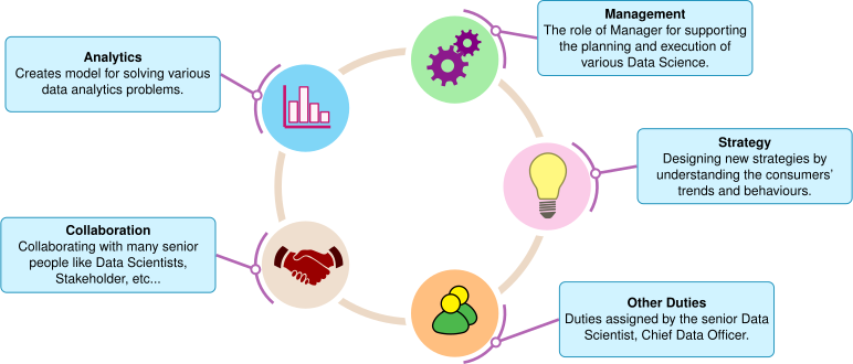](https://mlsysbook.ai/contents/core/ops/2487b8e52af58187faae03fa33647be0b0f08ce0.svg "Figure 8: AI Development Strategies: Model-centric and data-centric approaches represent complementary strategies for improving AI system performance; model-centric AI prioritizes architectural innovation, while data-centric AI focuses on enhancing data quality and representativeness to drive model improvements. Effective AI systems often require coordinated investment in both model and data improvements to achieve optimal results.")
Figure 8: **AI Development Strategies**: Model-centric and data-centric approaches represent complementary strategies for improving AI system performance; model-centric AI prioritizes architectural innovation, while data-centric AI focuses on enhancing data quality and representativeness to drive model improvements. Effective AI systems often require coordinated investment in both model and data improvements to achieve optimal results.
Following the MLOps principles established in [Section 1.2.2](https://mlsysbook.ai/contents/core/ops/ops.html#sec-ml-operations-mlops-c12b)
, these specialized roles align around a shared objective: delivering reliable, scalable, and maintainable machine learning systems in production environments. From designing robust data pipelines to deploying and monitoring models in live systems, effective collaboration depends on the disciplinary coordination that MLOps facilitates across data engineering, statistical modeling, software development, infrastructure management, and project coordination.
### Roles
[Table 4](https://mlsysbook.ai/contents/core/ops/ops.html#tbl-mlops-roles)
introduces the key roles that participate in MLOps and outlines their primary responsibilities. Understanding these roles not only clarifies the scope of skills required to support production ML systems but also helps frame the collaborative workflows and handoffs that drive the operational success of machine learning at scale.
Table 4: **MLOps Roles & Responsibilities**: Effective machine learning system operation requires a collaborative team with clearly defined roles (data engineers, data scientists, and others), each contributing specialized expertise throughout the entire lifecycle from data preparation to model deployment and monitoring. Understanding these roles clarifies skill requirements and promotes efficient workflows for scaling machine learning solutions.
| | | | |
| --- | --- | --- | --- |
| **Data Engineer** | Data preparation and infrastructure | Build and maintain pipelines; ensure quality, structure, and lineage of data | Data ingestion, transformation |
| **Data Scientist** | Model development and experimentation | Formulate tasks; build and evaluate models; iterate using feedback and error analysis | Modeling and evaluation |
| **ML Engineer** | Production integration and scalability | Operationalize models; implement serving logic; manage performance and retraining | Deployment and inference |
| **DevOps Engineer** | Infrastructure orchestration and automation | Manage compute infrastructure; implement CI/CD; monitor systems and workflows | Training, deployment, monitoring |
| **Project Manager** | Coordination and delivery oversight | Align goals; manage schedules and milestones; enable cross-team execution | Planning and integration |
| **Responsible AI** | Ethics, fairness, and governance | Monitor bias and fairness; enforce transparency and | Evaluation and governance |
| **Lead** | | compliance standards | |
| **Security & Privacy** | System protection and data integrity | Secure data and models; implement privacy controls; | Data handling and compliance |
| **Engineer** | | ensure system resilience | |
#### Data Engineers
Data engineers are responsible for constructing and maintaining the data infrastructure that underpins machine learning systems. Their primary focus is to ensure that data is reliably collected, processed, and made accessible in formats suitable for analysis, feature extraction, model training, and inference. In the context of MLOps, data engineers play a foundational role by building the **data infrastructure** components discussed earlier, including feature stores, data versioning systems, and validation frameworks, that enable scalable and reproducible data pipelines supporting the end-to-end machine learning lifecycle.
A core responsibility of data engineers is data ingestion: extracting data from diverse operational sources such as transactional databases, web applications, log streams, and sensors. This data is typically transferred to centralized storage systems, such as cloud-based object stores (e.g., Amazon S3, Google Cloud Storage), which provide scalable and durable repositories for both raw and processed datasets. These ingestion workflows are orchestrated using scheduling and workflow tools such as Apache Airflow, Prefect, or dbt ([Kampakis 2020](https://mlsysbook.ai/contents/core/ops/ops.html#ref-garg2020practical)
).
Kampakis, Stylianos. 2020. _The Decision Maker’s Handbook to Data Science: A Guide for Non-Technical Executives, Managers, and Founders_. Berkeley, CA: Apress. [https://doi.org/10.1007/978-1-4842-5494-3](https://doi.org/10.1007/978-1-4842-5494-3)
.
Once ingested, the data must be transformed into structured, analysis-ready formats. This transformation process includes handling missing or malformed values, resolving inconsistencies, performing joins across heterogeneous sources, and computing derived attributes required for downstream tasks. Data engineers implement these transformations through modular pipelines that are version-controlled and designed for fault tolerance and reusability. Structured outputs are often loaded into cloud-based data warehouses such as Snowflake, Redshift, or BigQuery, or stored in feature stores for use in machine learning applications.
In addition to managing data pipelines, data engineers are responsible for provisioning and optimizing the infrastructure that supports data-intensive workflows. This includes configuring distributed storage systems, managing compute clusters, and maintaining metadata catalogs that document data schemas, lineage, and access controls. To ensure reproducibility and governance, data engineers implement dataset versioning, maintain historical snapshots, and enforce data retention and auditing policies.
For example, in a manufacturing application, data engineers may construct an Airflow pipeline that ingests time-series sensor data from programmable logic controllers (PLCs)[39](https://mlsysbook.ai/contents/core/ops/ops.html#fn39)
on the factory floor.
39 **Programmable Logic Controllers (PLCs)**: Industrial computers designed to control manufacturing processes, machines, and assembly lines. PLCs process thousands of sensor inputs per second with microsecond-level timing precision, forming the backbone of automated manufacturing systems worth over $80 billion globally.
The raw data is cleaned, joined with product metadata, and aggregated into statistical features such as rolling averages and thresholds. The processed features are stored in a Snowflake data warehouse, where they are consumed by downstream modeling and inference workflows.
Through their design and maintenance of robust data infrastructure, data engineers enable the consistent and efficient delivery of high-quality data. Their contributions ensure that machine learning systems are built on reliable inputs, supporting reproducibility, scalability, and operational stability across the MLOps pipeline.
To illustrate this responsibility in practice, [Listing 1](https://mlsysbook.ai/contents/core/ops/ops.html#lst-data-engineer)
shows a simplified example of a daily Extract-Transform-Load (ETL) pipeline implemented using Apache Airflow. This workflow automates the ingestion and transformation of raw sensor data, preparing it for downstream machine learning tasks.
Listing 1: **Daily ETL Pipeline**: Automates the ingestion and transformation of raw sensor data for downstream ML tasks, highlighting the role of apache airflow in orchestrating workflow tasks.
# Airflow DAG for daily ETL from a manufacturing data source
from airflow import DAG
from airflow.operators.python import PythonOperator
from datetime import datetime
def extract_data():
import pandas as pd
df = pd.read_csv("/data/raw/plc_logs.csv")
# Simulated PLC data
df.to_parquet("/data/staged/sensor_data.parquet")
def transform_data():
import pandas as pd
df = pd.read_parquet("/data/staged/sensor_data.parquet")
df["rolling_avg"] = df["temperature"].rolling(window=10).mean()
df.to_parquet("/data/processed/features.parquet")
with DAG(
dag_id="manufacturing_etl_pipeline",
schedule_interval="@daily",
start_date=datetime(2023, 1, 1),
catchup=False,
) as dag:
extract = PythonOperator(
task_id="extract", python_callable=extract_data
)
transform = PythonOperator(
task_id="transform", python_callable=transform_data
)
extract >> transform
#### Data Scientists
Data scientists are responsible for designing, developing, and evaluating machine learning models. Their role centers on transforming business or operational problems into formal learning tasks, selecting appropriate algorithms, and optimizing model performance through statistical and computational techniques. Within the MLOps lifecycle, data scientists operate at the intersection of exploratory analysis and model development, contributing directly to the creation of predictive or decision-making capabilities.
The process typically begins by collaborating with stakeholders to define the problem space and establish success criteria. This includes formulating the task in machine learning terms, including classification, regression, or forecasting, and identifying suitable evaluation metrics to quantify model performance. These metrics, such as accuracy, precision, recall, area under the curve (AUC), or F1 score, provide objective measures for comparing model alternatives and guiding iterative improvements ([Rainio, Teuho, and Klén 2024](https://mlsysbook.ai/contents/core/ops/ops.html#ref-rainio2024evaluation)
).
Rainio, Oona, Jarmo Teuho, and Riku Klén. 2024. “Evaluation Metrics and Statistical Tests for Machine Learning.” _Scientific Reports_ 14 (1): 6086. [https://doi.org/10.1038/s41598-024-56706-x](https://doi.org/10.1038/s41598-024-56706-x)
.
Data scientists conduct exploratory data analysis (EDA) to assess data quality, identify patterns, and uncover relationships that inform feature selection and engineering. This stage may involve statistical summaries, visualizations, and hypothesis testing to evaluate the data’s suitability for modeling. Based on these findings, relevant features are constructed or selected in collaboration with data engineers to ensure consistency across development and deployment environments.
Model development involves selecting appropriate learning algorithms and constructing architectures suited to the task and data characteristics. Data scientists employ machine learning libraries such as TensorFlow, PyTorch, or scikit-learn to implement and train models. Hyperparameter tuning, regularization strategies, and cross-validation are used to optimize performance on validation datasets while mitigating overfitting. Throughout this process, tools for experiment tracking, including MLflow and Weights & Biases, are often used to log configuration settings, evaluation results, and model artifacts.
Once a candidate model demonstrates acceptable performance, it undergoes validation through testing on holdout datasets. In addition to aggregate performance metrics, data scientists perform error analysis to identify failure modes, outliers, or biases that may impact model reliability or fairness. These insights often motivate iterations on data processing, feature engineering, or model refinement.
Data scientists also participate in post-deployment monitoring and retraining workflows. They assist in analyzing data drift, interpreting shifts in model performance, and incorporating new data to maintain predictive accuracy over time. In collaboration with ML engineers, they define retraining strategies and evaluate the impact of updated models on operational metrics.
For example, in a retail forecasting scenario, a data scientist may develop a sequence model using TensorFlow to predict product demand based on historical sales, product attributes, and seasonal indicators. The model is evaluated using root mean squared error (RMSE) on withheld data, refined through hyperparameter tuning, and handed off to ML engineers for deployment. Following deployment, the data scientist continues to monitor model accuracy and guides retraining using new transactional data.
Through experimentation and model development, data scientists contribute the core analytical functionality of machine learning systems. Their work transforms raw data into predictive insights and supports the continuous improvement of deployed models through evaluation and refinement.
To illustrate these responsibilities in a practical context, [Listing 2](https://mlsysbook.ai/contents/core/ops/ops.html#lst-data-scientist)
presents a minimal example of a sequence model built using TensorFlow. This model is designed to forecast product demand based on historical sales patterns and other input features.
Listing 2: **Sequence Model**: A sequence model architecture can forecast future product demand based on historical sales patterns and other features, highlighting the importance of time-series data in predictive modeling through This example.
# TensorFlow model for demand forecasting
import tensorflow as tf
from tensorflow.keras import layers, models
model = models.Sequential(
[\
layers.Input(shape=(30, 5)),\
# 30 time steps, 5 features\
layers.LSTM(64),\
layers.Dense(1),\
]
)
model.compile(optimizer="adam", loss="mse", metrics=["mae"])
# Assume X_train, y_train are preloaded
model.fit(X_train, y_train, validation_split=0.2, epochs=10)
# Save model for handoff
model.save("models/demand_forecast_v1")
#### ML Engineers
Machine learning engineers are responsible for translating experimental models into reliable, scalable systems that can be integrated into real-world applications. Positioned at the intersection of data science and software engineering, ML engineers ensure that models developed in research environments can be deployed, monitored, and maintained within production infrastructure. Their work bridges the gap between prototyping and operationalization, enabling machine learning to deliver sustained value in practice.
A core responsibility of ML engineers is to take trained models and encapsulate them within modular, maintainable components. This often involves refactoring code for robustness, implementing model interfaces, and building application programming interfaces (APIs) that expose model predictions to downstream systems. Frameworks such as Flask and FastAPI are commonly used to construct lightweight, RESTful services for model inference. To support portability and environment consistency, models and their dependencies are typically containerized using Docker and managed within orchestration systems like Kubernetes.
ML engineers also oversee the integration of models into **continuous pipelines** and implement the **deployment and serving** infrastructure discussed in the production operations section. These pipelines automate the retraining, testing, and deployment of models, ensuring that updated models are validated against performance benchmarks before being promoted to production. Practices such as the **canary testing** strategies outlined earlier, A/B testing, and staged rollouts allow for gradual transitions and reduce the risk of regressions. In the event of model degradation, rollback procedures are used to restore previously validated versions.
Operational efficiency is another key area of focus. ML engineers apply a range of optimization techniques, including model quantization, pruning, and batch serving, to meet latency, throughput, and cost constraints. In systems that support multiple models, they may implement mechanisms for dynamic model selection or concurrent serving. These optimizations are closely coupled with infrastructure provisioning, which often includes the configuration of GPUs or other specialized accelerators.
Post-deployment, ML engineers play a critical role in monitoring model behavior. They configure telemetry systems[40](https://mlsysbook.ai/contents/core/ops/ops.html#fn40)
to track latency, failure rates, and resource usage, and they instrument prediction pipelines with logging and alerting mechanisms.
40 **ML Telemetry**: Automated collection of operational data from ML systems including model performance metrics, infrastructure utilization, and prediction accuracy. Production ML systems generate 10 GB-1 TB of telemetry daily, enabling real-time drift detection and performance optimization.
In collaboration with data scientists and DevOps engineers, they respond to changes in system behavior, trigger retraining workflows, and ensure that models continue to meet service-level objectives.
For example, consider a financial services application where a data science team has developed a fraud detection model using TensorFlow. An ML engineer packages the model for deployment using TensorFlow Serving, configures a REST API for integration with the transaction pipeline, and sets up a CI/CD pipeline in Jenkins to automate updates. They implement logging and monitoring using Prometheus and Grafana, and configure rollback logic to revert to the prior model version if performance deteriorates. This production infrastructure enables the model to operate continuously and reliably under real-world workloads.
Through their focus on software robustness, deployment automation, and operational monitoring, ML engineers play a critical role in transitioning machine learning models from experimental artifacts into trusted components of production systems. These responsibilities vary significantly by organization size: at startups, ML engineers often span the entire stack from data pipeline development to model deployment, while at large technology companies like Meta or Google, they typically specialize in specific areas such as serving infrastructure or feature engineering. Mid-sized companies often have ML engineers owning end-to-end responsibility for specific model domains (e.g., recommendation systems), balancing breadth and specialization. To illustrate these responsibilities in a practical context, [Listing 3](https://mlsysbook.ai/contents/core/ops/ops.html#lst-ml-engineer)
presents a minimal example of a REST API built with FastAPI for serving a trained TensorFlow model. This service exposes model predictions for use in downstream applications.
Listing 3: **FastAPI Service**: Wraps a TensorFlow model to provide real-time demand predictions, illustrating how ML engineers integrate models into production systems.
# FastAPI service to serve a trained TensorFlow model
from fastapi import FastAPI, Request
import tensorflow as tf
import numpy as np
app = FastAPI()
model = tf.keras.models.load_model("models/demand_forecast_v1")
@app.post("/predict")
async def predict(request: Request):
data = await request.json()
input_array = np.array(data["input"]).reshape(1, 30, 5)
prediction = model.predict(input_array)
return {"prediction": float(prediction[0][0])}
#### DevOps Engineers
DevOps engineers are responsible for provisioning, managing, and automating the infrastructure that supports the development, deployment, and monitoring of machine learning systems. Originating from the broader discipline of software engineering, the role of the DevOps engineer in MLOps extends traditional responsibilities to accommodate the specific demands of data- and model-driven workflows. Their expertise in cloud computing, automation pipelines, and infrastructure as code (IaC) enables scalable and reliable machine learning operations.
A central task for DevOps engineers is the configuration and orchestration of compute infrastructure used throughout the ML lifecycle. This includes provisioning virtual machines, storage systems, and accelerators such as GPUs and TPUs using IaC tools like Terraform, AWS CloudFormation, or Ansible. Infrastructure is typically containerized using Docker and managed through orchestration platforms such as Kubernetes, which allow teams to deploy, scale, and monitor workloads across distributed environments.
DevOps engineers design and implement CI/CD pipelines tailored to machine learning workflows. These pipelines automate the retraining, testing, and deployment of models in response to code changes or data updates. Tools such as Jenkins, GitHub Actions, or GitLab CI are used to trigger model workflows, while platforms like MLflow and Kubeflow facilitate experiment tracking, model registration, and artifact versioning. By codifying deployment logic, these pipelines reduce manual effort, increase reproducibility, and enable faster iteration cycles.
Monitoring is another critical area of responsibility. DevOps engineers configure telemetry systems to collect metrics related to both model and infrastructure performance. Tools such as Prometheus, Grafana, and the ELK stack[41](https://mlsysbook.ai/contents/core/ops/ops.html#fn41)
(Elasticsearch, Logstash, Kibana) are widely used to build dashboards, set thresholds, and generate alerts.
41 **ELK Stack**: Elasticsearch (search/analytics engine), Logstash (data processing pipeline), and Kibana (visualization platform). Can process terabytes of logs daily with millisecond search response times. Used by Netflix to analyze 1+ billion events daily and identify system anomalies in real-time.
These systems allow teams to detect anomalies in latency, throughput, resource utilization, or prediction behavior and respond proactively to emerging issues.
To ensure compliance and operational discipline, DevOps engineers also implement governance mechanisms that enforce consistency and traceability. This includes versioning of infrastructure configurations, automated validation of deployment artifacts, and auditing of model updates. In collaboration with ML engineers and data scientists, they enable reproducible and auditable model deployments aligned with organizational and regulatory requirements.
For instance, in a financial services application, a DevOps engineer may configure a Kubernetes cluster on AWS to support both model training and online inference. Using Terraform, the infrastructure is defined as code and versioned alongside the application repository. Jenkins is used to automate the deployment of models registered in MLflow, while Prometheus and Grafana provide real-time monitoring of API latency, resource usage, and container health.
By abstracting and automating the infrastructure that underlies ML workflows, DevOps engineers enable scalable experimentation, robust deployment, and continuous monitoring. Their role ensures that machine learning systems can operate reliably under production constraints, with minimal manual intervention and maximal operational efficiency. To illustrate these responsibilities in a practical context, [Listing 4](https://mlsysbook.ai/contents/core/ops/ops.html#lst-devops-engineer)
presents an example of using Terraform to provision a GPU-enabled virtual machine on Google Cloud Platform for model training and inference workloads.
Listing 4: **GPU-Enabled Infrastructure**: This configuration ensures efficient model training and inference by leveraging a specific machine type and GPU accelerator on Google cloud platform.
# Terraform configuration for a GCP instance with GPU support
resource "google_compute_instance" "ml_node" {
name = "ml-gpu-node"
machine_type = "n1-standard-8"
zone = "us-central1-a"
boot_disk {
initialize_params {
image = "debian-cloud/debian-11"
}
}
guest_accelerator {
type = "nvidia-tesla-t4"
count = 1
}
metadata_startup_script = <<-EOF
sudo apt-get update
sudo apt-get install -y docker.io
sudo docker run --gpus all -p 8501:8501 tensorflow/serving
EOF
tags = ["ml-serving"]
}
#### Project Managers
Project managers play a critical role in coordinating the activities, resources, and timelines involved in delivering machine learning systems. While they do not typically develop models or write code, project managers are essential to aligning interdisciplinary teams, tracking progress against objectives, and ensuring that MLOps initiatives are completed on schedule and within scope. Their work enables effective collaboration among data scientists, engineers, product stakeholders, and infrastructure teams, translating business goals into actionable technical plans.
At the outset of a project, project managers work with organizational stakeholders to define goals, success metrics, and constraints. This includes clarifying the business objectives of the machine learning system, identifying key deliverables, estimating timelines, and setting performance benchmarks. These definitions serve as the foundation for resource allocation, task planning, and risk assessment throughout the lifecycle of the project.
Once the project is initiated, project managers are responsible for developing and maintaining a detailed execution plan. This plan outlines major phases of work, such as data collection, model development, infrastructure provisioning, deployment, and monitoring. Dependencies between tasks are identified and managed to ensure smooth handoffs between roles, while milestones and checkpoints are used to assess progress and adjust schedules as necessary.
Throughout execution, project managers facilitate coordination across teams. This includes organizing meetings, tracking deliverables, resolving blockers, and escalating issues when necessary. Documentation, progress reports, and status updates are maintained to provide visibility across the organization and ensure that all stakeholders are informed of project developments. Communication is a central function of the role, serving to reduce misalignment and clarify expectations between technical contributors and business decision-makers.
In addition to managing timelines and coordination, project managers oversee the budgeting and resourcing aspects of MLOps initiatives. This may involve evaluating cloud infrastructure costs, negotiating access to compute resources, and ensuring that appropriate personnel are assigned to each phase of the project. By maintaining visibility into both technical and organizational considerations, project managers help align technical execution with strategic priorities.
For example, consider a company seeking to reduce customer churn using a predictive model. The project manager coordinates with data engineers to define data requirements, with data scientists to prototype and evaluate models, with ML engineers to package and deploy the final model, and with DevOps engineers to provision the necessary infrastructure and monitoring tools. The project manager tracks progress through phases such as data pipeline readiness, baseline model evaluation, deployment to staging, and post-deployment monitoring, adjusting the project plan as needed to respond to emerging challenges.
By orchestrating collaboration across diverse roles and managing the complexity inherent in machine learning initiatives, project managers enable MLOps teams to deliver systems that are both technically robust and aligned with organizational goals. Their contributions ensure that the operationalization of machine learning is not only feasible, but repeatable, accountable, and efficient. To illustrate these responsibilities in a practical context, [Listing 5](https://mlsysbook.ai/contents/core/ops/ops.html#lst-project-manager)
presents a simplified example of a project milestone tracking structure using JSON. This format is commonly used to integrate with tools like JIRA or project dashboards to monitor progress across machine learning initiatives.
Listing 5: **Milestone Tracking Structure**: This JSON format organizes project phases like data readiness and model deployment, highlighting progress and risk management for machine learning initiatives.
{
"project": "Churn Prediction",
"milestones": [\
{\
"name": "Data Pipeline Ready",\
"due": "2025-05-01",\
"status": "Complete",\
},\
{\
"name": "Model Baseline",\
"due": "2025-05-10",\
"status": "In Progress",\
},\
{\
"name": "Staging Deployment",\
"due": "2025-05-15",\
"status": "Pending",\
},\
{\
"name": "Production Launch",\
"due": "2025-05-25",\
"status": "Pending",\
},\
],
"risks": [\
{\
"issue": "Delayed cloud quota",\
"mitigation": "Request early from infra team",\
}\
],
}
#### Responsible AI Lead
The Responsible AI Lead is tasked with ensuring that machine learning systems operate in ways that are transparent, fair, accountable, and compliant with ethical and regulatory standards. As machine learning is increasingly embedded in socially impactful domains such as healthcare, finance, and education, the need for systematic governance has grown. This role reflects a growing recognition that technical performance alone is insufficient; ML systems must also align with broader societal values.
At the model development stage, Responsible AI Leads support practices that enhance interpretability and transparency. They work with data scientists and ML engineers to assess which features contribute most to model predictions, evaluate whether certain groups are disproportionately affected, and document model behavior through structured reporting mechanisms. Post hoc explanation methods, such as attribution techniques, are often reviewed in collaboration with this role to support downstream accountability.
Another key responsibility is fairness assessment. This involves defining fairness criteria in collaboration with stakeholders, auditing model outputs for performance disparities across demographic groups, and guiding interventions, including reweighting, re-labeling, or constrained optimization, to mitigate potential harms. These assessments are often incorporated into model validation pipelines to ensure that they are systematically enforced before deployment.
In post-deployment settings, Responsible AI Leads help monitor systems for drift, bias amplification, and unanticipated behavior. They may also oversee the creation of documentation artifacts such as model cards or datasheets for datasets, which serve as tools for transparency and reproducibility. In regulated sectors, this role collaborates with legal and compliance teams to meet audit requirements and ensure that deployed models remain aligned with external mandates.
For example, in a hiring recommendation system, a Responsible AI Lead may oversee an audit that compares model outcomes across gender and ethnicity, guiding the team to adjust the training pipeline to reduce disparities while preserving predictive accuracy. They also ensure that decision rationales are documented and reviewable by both technical and non-technical stakeholders.
The integration of ethical review and governance into the ML development process enables the Responsible AI Lead to support systems that are not only technically robust, but also socially responsible and institutionally accountable. To illustrate these responsibilities in a practical context, [Listing 6](https://mlsysbook.ai/contents/core/ops/ops.html#lst-responsible-ai)
presents an example of using the Aequitas library to audit a model for group-based disparities. This example evaluates statistical parity across demographic groups to assess potential fairness concerns prior to deployment.
Listing 6: **Fairness Audit**: Evaluates model outcomes to identify gender disparities using aequitas, ensuring socially responsible AI systems.
# Fairness audit using Aequitas
from aequitas.group import Group
from aequitas.bias import Bias
# Assume df includes model scores, true labels,
# and a 'gender' attribute
g = Group().get_crosstabs(df)
b = Bias().get_disparity_predefined_groups(
g,
original_df=df,
ref_groups_dict={"gender": "male"},
alpha=0.05,
mask_significant=True,
)
print(
b[\
[\
"attribute_name",\
"attribute_value",\
"disparity",\
"statistical_parity",\
]\
]
)
#### Security and Privacy Engineer
The Security and Privacy Engineer is responsible for safeguarding machine learning systems against adversarial threats and privacy risks. As ML systems increasingly rely on sensitive data and are deployed in high-stakes environments, security and privacy become essential dimensions of system reliability. This role brings expertise in both traditional security engineering and ML-specific threat models, ensuring that systems are resilient to attack and compliant with data protection requirements.
At the data level, Security and Privacy Engineers help enforce access control, encryption, and secure handling of training and inference data. They collaborate with data engineers to apply privacy-preserving techniques, such as data anonymization, secure aggregation, or differential privacy, particularly when sensitive personal or proprietary data is used. These mechanisms are designed to reduce the risk of data leakage while retaining the utility needed for model training.
In the modeling phase, this role advises on techniques that improve robustness against adversarial manipulation. This may include detecting poisoning attacks during training, mitigating model inversion or membership inference risks, and evaluating the susceptibility of models to adversarial examples. They also assist in designing model architectures and training strategies that balance performance with safety constraints.
During deployment, Security and Privacy Engineers implement controls to protect the model itself, including endpoint hardening, API rate limiting, and access logging. In settings where models are exposed externally, including public-facing APIs, they may also deploy monitoring systems that detect anomalous access patterns or query-based attacks intended to extract model parameters or training data.
For instance, in a medical diagnosis system trained on patient data, a Security and Privacy Engineer might implement differential privacy during model training and enforce strict access controls on the model’s inference interface. They would also validate that model explanations do not inadvertently expose sensitive information, and monitor post-deployment activity for potential misuse.
Through proactive design and continuous oversight, Security and Privacy Engineers ensure that ML systems uphold confidentiality, integrity, and availability. Their work is especially critical in domains where trust, compliance, and risk mitigation are central to system deployment and long-term operation. To illustrate these responsibilities in a practical context, [Listing 7](https://mlsysbook.ai/contents/core/ops/ops.html#lst-security-privacy)
presents an example of training a model using differential privacy techniques with TensorFlow Privacy. This approach helps protect sensitive information in the training data while preserving model utility.
Listing 7: **Differentially Private Training**: To train a machine learning model using differential privacy techniques in TensorFlow Privacy, ensuring sensitive data protection while maintaining predictive performance via This code snippet. _Source: TensorFlow Privacy Documentation_
# Training a differentially private model with
# TensorFlow Privacy
import tensorflow as tf
from tensorflow_privacy.privacy.optimizers.dp_optimizer_keras import (
DPKerasAdamOptimizer,
)
# Define a simple model
model = tf.keras.Sequential(
[\
tf.keras.layers.Dense(\
64, activation="relu", input_shape=(100,)\
),\
tf.keras.layers.Dense(10, activation="softmax"),\
]
)
# Use a DP-aware optimizer
optimizer = DPKerasAdamOptimizer(
l2_norm_clip=1.0,
noise_multiplier=1.1,
num_microbatches=256,
learning_rate=0.001,
)
model.compile(
optimizer=optimizer,
loss="categorical_crossentropy",
metrics=["accuracy"],
)
# Train model on privatized dataset
model.fit(train_data, train_labels, epochs=10, batch_size=256)
### Intersections and Handoffs
While each role in MLOps carries distinct responsibilities, the successful deployment and operation of machine learning systems depends on seamless collaboration across functional boundaries. Machine learning workflows are inherently interdependent, with critical handoff points connecting data acquisition, model development, system integration, and operational monitoring. Understanding these intersections is essential for designing processes that are both efficient and resilient.
One of the earliest and most critical intersections occurs between data engineers and data scientists. Data engineers construct and maintain the pipelines that ingest and transform raw data, while data scientists depend on these pipelines to access clean, structured, and well-documented datasets for analysis and modeling. Misalignment at this stage, including undocumented schema changes or inconsistent feature definitions, can lead to downstream errors that compromise model quality or reproducibility.
Once a model is developed, the handoff to ML engineers requires a careful transition from research artifacts to production-ready components. ML engineers must understand the assumptions and requirements of the model to implement appropriate interfaces, optimize runtime performance, and integrate it into the broader application ecosystem. This step often requires iteration, especially when models developed in experimental environments must be adapted to meet latency, throughput, or resource constraints in production.
As models move toward deployment, DevOps engineers play the role in provisioning infrastructure, managing CI/CD pipelines, and instrumenting monitoring systems. Their collaboration with ML engineers ensures that model deployments are automated, repeatable, and observable. They also coordinate with data scientists to define alerts and thresholds that guide performance monitoring and retraining decisions.
Project managers provide the organizational glue across these technical domains. They ensure that handoffs are anticipated, roles are clearly defined, and dependencies are actively managed. In particular, project managers help maintain continuity by documenting assumptions, tracking milestone readiness, and facilitating communication between teams. This coordination reduces friction and enables iterative development cycles that are both agile and accountable.
For example, in a real-time recommendation system, data engineers maintain the data ingestion pipeline and feature store, data scientists iterate on model architectures using historical clickstream data, ML engineers deploy models as containerized microservices[42](https://mlsysbook.ai/contents/core/ops/ops.html#fn42)
, and DevOps engineers monitor inference latency and availability.
42 **Microservices in ML**: Architectural pattern where each ML model runs as an independent, loosely-coupled service with its own database and deployment lifecycle. Netflix operates 700+ microservices including 100+ for ML recommendations, enabling independent scaling and faster experimentation cycles.
Each role contributes to a different layer of the stack, but the overall functionality depends on reliable transitions between each phase of the lifecycle. These role interactions illustrate that MLOps is not simply a collection of discrete tasks, but a continuous, collaborative process ([Figure 9](https://mlsysbook.ai/contents/core/ops/ops.html#fig-mlops-handoffs)
). Designing for clear handoffs, shared tools, and well-defined interfaces is essential for ensuring that machine learning systems can evolve, scale, and perform reliably over time.
[](https://mlsysbook.ai/contents/core/ops/ab8b862b0652a0a14491ca1469d9c53836030cb2.svg "Figure 9: MLOps Role Handoffs Workflow: Machine learning workflows require systematic handoffs between specialized roles, with each role producing specific artifacts that become inputs for downstream activities. Critical handoff points (H1-H3) represent coordination moments where clear interfaces, shared understanding, and documented requirements become essential for system reliability. Feedback loops enable continuous improvement based on production performance data.")
Figure 9: **MLOps Role Handoffs Workflow**: Machine learning workflows require systematic handoffs between specialized roles, with each role producing specific artifacts that become inputs for downstream activities. Critical handoff points (H1-H3) represent coordination moments where clear interfaces, shared understanding, and documented requirements become essential for system reliability. Feedback loops enable continuous improvement based on production performance data.
### Evolving Roles and Specializations
As machine learning systems mature and organizations adopt MLOps practices at scale, the structure and specialization of roles often evolve. In early-stage environments, individual contributors may take on multiple responsibilities, such as a data scientist who also builds data pipelines or manages model deployment. However, as systems grow in complexity and teams expand, responsibilities tend to become more differentiated, giving rise to new roles and more structured organizational patterns.
One emerging trend is the formation of dedicated ML platform teams, which focus on building shared infrastructure and tooling to support experimentation, deployment, and monitoring across multiple projects. These teams often abstract common workflows, including data versioning, model training orchestration, and CI/CD integration, into reusable components or internal platforms. This approach reduces duplication of effort and accelerates development by enabling application teams to focus on domain-specific problems rather than underlying systems engineering.
In parallel, hybrid roles have emerged to bridge gaps between traditional boundaries. For example, full-stack ML engineers combine expertise in modeling, software engineering, and infrastructure to own the end-to-end deployment of ML models. Similarly, ML enablement roles, including MLOps engineers and applied ML specialists, focus on helping teams adopt best practices, integrate tooling, and scale workflows efficiently. These roles are especially valuable in organizations with diverse teams that vary in ML maturity or technical specialization.
The structure of MLOps teams also varies based on organizational scale, industry, and regulatory requirements. In smaller organizations or startups, teams are often lean and cross-functional, with close collaboration and informal processes. In contrast, larger enterprises may formalize roles and introduce governance frameworks to manage compliance, data security, and model risk. Highly regulated sectors, including finance, healthcare, and defense, often require additional roles focused on validation, auditing, and documentation to meet external reporting obligations.
As [Table 5](https://mlsysbook.ai/contents/core/ops/ops.html#tbl-mlops-evolution)
indicates, the boundaries between roles are not rigid. Effective MLOps practices rely on shared understanding, documentation, and tools that facilitate communication and coordination across teams. Encouraging interdisciplinary fluency, including enabling data scientists to understand deployment workflows and DevOps engineers to interpret model monitoring metrics, enhances organizational agility and resilience.
Table 5: **Role Evolution**: MLOps roles increasingly specialize as systems mature, demanding cross-functional collaboration between data engineers, data scientists, and ML engineers to bridge data preparation, model building, and deployment challenges. Expanding responsibilities, such as feature store management and model validation, reflect the growing need for robust, ethical, and scalable machine learning infrastructure.
| | | |
| --- | --- | --- |
| **Data Engineer** | Works with data scientists to define features and pipelines | Expands into real-time data systems and feature store platforms |
| **Data Scientist** | Relies on data engineers for clean inputs; collaborates with ML engineers | Takes on model validation, interpretability, and ethical considerations |
| **ML Engineer** | Receives models from data scientists; works with DevOps to deploy and monitor | Transitions into platform engineering or full-stack ML roles |
| **DevOps Engineer** | Supports ML engineers with infrastructure, CI/CD, and observability | Evolves into MLOps platform roles; integrates governance and security tooling |
| **Project Manager** | Coordinates across all roles; tracks progress and communication | Specializes into ML product management as systems scale |
| **Responsible AI Lead** | Collaborates with data scientists and PMs to evaluate fairness and compliance | Role emerges as systems face regulatory scrutiny or public exposure |
| **Security & Privacy** | Works with DevOps and ML Engineers to | Role formalizes as privacy regulations |
| **Engineer** | secure data pipelines and model interfaces | (e.g., GDPR, HIPAA) apply to ML workflows |
As machine learning becomes increasingly central to modern software systems, roles will continue to adapt in response to emerging tools, methodologies, and system architectures. Recognizing the dynamic nature of these responsibilities allows teams to allocate resources effectively, design adaptable workflows, and foster collaboration that is essential for sustained success in production-scale machine learning.
The specialized roles and cross-functional collaboration patterns described above do not emerge in isolation. They evolve alongside the technical and organizational maturity of ML systems themselves. Understanding this co-evolution between roles, infrastructure, and operational practices provides essential context for designing sustainable MLOps implementations.
**Self-Check: Question 1.6**
1. Which role is primarily responsible for ensuring data quality and managing data pipelines in an MLOps framework?
1. Data Scientist
2. ML Engineer
3. DevOps Engineer
4. Data Engineer
2. Explain how the handoff between Data Scientists and ML Engineers is critical for successful model deployment in MLOps.
3. True or False: In an MLOps framework, DevOps Engineers are primarily responsible for model development and experimentation.
4. Order the following roles based on their typical involvement in the MLOps lifecycle from data preparation to deployment: (1) Data Engineer, (2) ML Engineer, (3) Data Scientist, (4) DevOps Engineer.
[See Answers →](https://mlsysbook.ai/contents/core/ops/ops.html#quiz-answer-sec-ml-operations-roles-responsibilities-79d5)
System Design and Maturity Framework
------------------------------------
Building on the infrastructure components, production operations, and organizational roles established earlier, we now examine how these elements integrate into coherent operational systems. Machine learning systems do not operate in isolation. Their effectiveness depends not only on the quality of the underlying models, but also on the maturity of the organizational and technical processes that support them. This section explores how operational maturity shapes system architecture and provides frameworks for designing MLOps implementations that address the operational challenges identified at the chapter’s beginning. Operational maturity refers to the degree to which ML workflows are automated, reproducible, monitored, and aligned with broader engineering and governance practices. While early-stage efforts may rely on ad hoc scripts and manual interventions, production-scale systems require deliberate design choices that support long-term sustainability, reliability, and adaptability. This section examines how different levels of operational maturity influence system architecture, infrastructure design, and organizational structure, providing a lens through which to interpret the broader MLOps landscape ([Paleyes, Urma, and Lawrence 2022](https://mlsysbook.ai/contents/core/ops/ops.html#ref-kreuzberger2022machine)
).
Paleyes, Andrei, Raoul-Gabriel Urma, and Neil D. Lawrence. 2022. “Challenges in Deploying Machine Learning: A Survey of Case Studies.” _ACM Computing Surveys_ 55 (6): 1–29. [https://doi.org/10.1145/3533378](https://doi.org/10.1145/3533378)
.
### Operational Maturity
Operational maturity in machine learning refers to the extent to which an organization can reliably develop, deploy, and manage ML systems in a repeatable and scalable manner. Unlike the maturity of individual models or algorithms, operational maturity reflects systemic capabilities: how well a team or organization integrates infrastructure, automation, monitoring, governance, and collaboration into the ML lifecycle.
Low-maturity environments often rely on manual workflows, loosely coupled components, and ad hoc experimentation. While sufficient for early-stage research or low-risk applications, such systems tend to be brittle, difficult to reproduce, and highly sensitive to data or code changes. As ML systems are deployed at scale, these limitations quickly become barriers to sustained performance, trust, and accountability.
In contrast, high-maturity environments implement modular, versioned, and automated workflows that allow models to be developed, validated, and deployed in a controlled and observable fashion. Data lineage is preserved across transformations; model behavior is continuously monitored and evaluated; and infrastructure is provisioned and managed as code. These practices reduce operational friction, enable faster iteration, and support robust decision-making in production ([A. Chen et al. 2020](https://mlsysbook.ai/contents/core/ops/ops.html#ref-zaharia2018accelerating)
).
Chen, Andrew, Andy Chow, Aaron Davidson, Arjun DCunha, Ali Ghodsi, Sue Ann Hong, Andy Konwinski, et al. 2020. “Developments in MLflow: A System to Accelerate the Machine Learning Lifecycle.” In _Proceedings of the Fourth International Workshop on Data Management for End-to-End Machine Learning_, 1–4. ACM. [https://doi.org/10.1145/3399579.3399867](https://doi.org/10.1145/3399579.3399867)
.
Operational maturity is not solely a function of tool adoption. While technologies such as CI/CD pipelines, model registries, and observability stacks play a role, maturity centers on system integration and coordination: how data engineers, data scientists, and operations teams collaborate through shared interfaces, standardized workflows, and automated handoffs. It is this integration that distinguishes mature ML systems from collections of loosely connected artifacts.
### Maturity Levels
While operational maturity exists on a continuum, it is useful to distinguish between broad stages that reflect how ML systems evolve from research prototypes to production-grade infrastructure. These stages are not strict categories, but rather indicative of how organizations gradually adopt practices that support reliability, scalability, and observability.
At the lowest level of maturity, ML workflows are ad hoc: experiments are run manually, models are trained on local machines, and deployment involves hand-crafted scripts or manual intervention. Data pipelines may be fragile or undocumented, and there is limited ability to trace how a deployed model was produced. These environments may be sufficient for prototyping, but they are ill-suited for ongoing maintenance or collaboration.
As maturity increases, workflows become more structured and repeatable. Teams begin to adopt version control, automated training pipelines, and centralized model storage. Monitoring and testing frameworks are introduced, and retraining workflows become more systematic. Systems at this level can support limited scale and iteration but still rely heavily on human coordination.
At the highest levels of maturity, ML systems are fully integrated with infrastructure-as-code, continuous delivery pipelines, and automated monitoring. Data lineage, feature reuse, and model validation are encoded into the development process. Governance is embedded throughout the system, allowing for traceability, auditing, and policy enforcement. These environments support large-scale deployment, rapid experimentation, and adaptation to changing data and system conditions.
This progression, summarized in [Table 6](https://mlsysbook.ai/contents/core/ops/ops.html#tbl-maturity-levels)
, offers a system-level framework for analyzing ML operational practices. It emphasizes architectural cohesion and lifecycle integration over tool selection, guiding the design of scalable and maintainable learning systems.
| | | |
| --- | --- | --- |
| **Ad Hoc** | Manual data processing, local training, no version control, unclear ownership | Fragile workflows, difficult to reproduce or debug |
| **Repeatable** | Automated training pipelines, basic CI/CD, centralized model storage, some monitoring | Improved reproducibility, limited scalability |
| **Scalable** | Fully automated workflows, integrated observability, infrastructure-as-code, governance | High reliability, rapid iteration, production-grade ML |
These maturity levels provide a systems lens through which to evaluate ML operations, not in terms of specific tools adopted, but in how reliably and cohesively a system supports the full machine learning lifecycle. Understanding this progression prepares practitioners to identify design bottlenecks and prioritize investments that support long-term system sustainability.
Table 6: **Maturity Progression**: Machine learning operational practices evolve from manual, fragile workflows toward fully integrated, automated systems, impacting reproducibility and scalability. This table outlines key characteristics and outcomes at different maturity levels, emphasizing architectural cohesion and lifecycle integration for building maintainable learning systems.
| | | |
| --- | --- | --- |
| **Ad Hoc** | Manual data processing, local training, no version control, unclear ownership | Fragile workflows, difficult to reproduce or debug |
| **Repeatable** | Automated training pipelines, basic CI/CD, centralized model storage, some monitoring | Improved reproducibility, limited scalability |
| **Scalable** | Fully automated workflows, integrated observability, infrastructure-as-code, governance | High reliability, rapid iteration, production-grade ML |
### System Design Implications
As machine learning operations mature, the underlying system architecture evolves in response. Operational maturity is not just an organizational concern; it has direct consequences for how ML systems are structured, deployed, and maintained. Each level of maturity introduces new expectations around modularity, automation, monitoring, and fault tolerance, shaping the design space in both technical and procedural terms.
In low-maturity environments, ML systems are often constructed around monolithic scripts and tightly coupled components. Data processing logic may be embedded directly within model code, and configurations are managed informally. These architectures, while expedient for rapid experimentation, lack the separation of concerns needed for maintainability, version control, or safe iteration. As a result, teams frequently encounter regressions, silent failures, and inconsistent performance across environments.
As maturity increases, modular abstractions begin to emerge. Feature engineering is decoupled from model logic, pipelines are defined declaratively, and system boundaries are enforced through APIs and orchestration frameworks. These changes support reproducibility and enable teams to scale development across multiple contributors or applications. Infrastructure becomes programmable through configuration files, and model artifacts are promoted through standardized deployment stages. This architectural discipline allows systems to evolve predictably, even as requirements shift or data distributions change.
At high levels of maturity, ML systems exhibit properties commonly found in production-grade software systems: stateless services, contract-driven interfaces, environment isolation, and observable execution. Design patterns such as feature stores, model registries, and infrastructure-as-code become foundational. Crucially, system behavior is not inferred from static assumptions, but monitored in real time and adapted as needed. This enables feedback-driven development and supports closed-loop systems where data, models, and infrastructure co-evolve.
In each case, operational maturity is not an external constraint but an architectural force: it governs how complexity is managed, how change is absorbed, and how the system can scale in the face of threats to service uptime (see [Figure 10](https://mlsysbook.ai/contents/core/ops/ops.html#fig-uptime-iceberg)
). Design decisions that disregard these constraints may function under ideal conditions, but fail under real-world pressures such as latency requirements, drift, outages, or regulatory audits. Understanding this relationship between maturity and design is essential for building resilient machine learning systems that sustain performance over time.
[](https://mlsysbook.ai/contents/core/ops/17f8e37e5ff1dba6848e73e6efdbdb624d450639.svg "Figure 10: Uptime Dependency Stack: Robust ML service uptime relies on monitoring a layered stack of interdependent components, from infrastructure to model performance, mirroring the complexity of modern software systems. Operational maturity necessitates observing this entire stack to proactively address potential failures and maintain service levels under varying conditions.")
Figure 10: **Uptime Dependency Stack**: Robust ML service uptime relies on monitoring a layered stack of interdependent components, from infrastructure to model performance, mirroring the complexity of modern software systems. Operational maturity necessitates observing this entire stack to proactively address potential failures and maintain service levels under varying conditions.
### Design Patterns and Anti-Patterns
The structure of the teams involved in building and maintaining machine learning systems plays a significant role in determining operational outcomes. As ML systems grow in complexity and scale, organizational patterns must evolve to reflect the interdependence between data, modeling, infrastructure, and governance. While there is no single ideal structure, certain patterns consistently support operational maturity, whereas others tend to hinder it.
In mature environments, organizational design emphasizes clear ownership, cross-functional collaboration, and interface discipline between roles. For instance, platform teams may take responsibility for shared infrastructure, tooling, and CI/CD pipelines, while domain teams focus on model development and business alignment. This separation of concerns enables reuse, standardization, and parallel development. Interfaces between teams, including feature definitions, data schemas, and deployment targets, are well-defined and versioned, reducing friction and ambiguity.
One effective pattern is the creation of a centralized MLOps team that provides shared services to multiple model development groups. This team maintains tooling for model training, validation, deployment, and monitoring, and may operate as an internal platform provider. Such structures promote consistency, reduce duplicated effort, and accelerate onboarding for new projects. Alternatively, some organizations adopt a federated model, embedding MLOps engineers within product teams while maintaining a central architectural function to guide system-wide integration.
In contrast, anti-patterns often emerge when responsibilities are fragmented or poorly aligned. One common failure mode is the tool-first approach, in which teams adopt infrastructure or automation tools without first defining the processes and roles that should govern their use. This can result in fragile pipelines, unclear handoffs, and duplicated effort. Another anti-pattern is siloed experimentation, where data scientists operate in isolation from production engineers, leading to models that are difficult to deploy, monitor, or retrain effectively.
Organizational drift is another subtle challenge. As teams scale, undocumented workflows and informal agreements may become entrenched, increasing the cost of coordination and reducing transparency. Without deliberate system design and process review, even previously functional structures can accumulate technical and organizational debt.
Ultimately, organizational maturity must co-evolve with system complexity. Teams must establish communication patterns, role definitions, and accountability structures that reinforce the principles of modularity, automation, and observability. Operational excellence in machine learning is not just a matter of technical capability; it is the product of coordinated, intentional systems thinking across human and computational boundaries.
The organizational patterns described above must be supported by technical architectures that can handle the unique reliability challenges of ML systems. MLOps inherits many reliability challenges from distributed systems but adds unique complications through learning components. Traditional reliability patterns require adaptation to account for the probabilistic nature of ML systems and the dynamic behavior of learning components.
Circuit breaker patterns must account for model-specific failure modes, where prediction accuracy degradation requires different thresholds than service availability failures. Bulkhead patterns become critical when isolating experimental model versions from production traffic, requiring resource partitioning strategies that prevent resource exhaustion in one model from affecting others. The Byzantine fault tolerance problem takes on new characteristics in MLOps environments, where “Byzantine” behavior includes models producing plausible but incorrect outputs rather than obvious failures.
Traditional consensus algorithms focus on agreement among correct nodes, but ML systems require consensus about model correctness when ground truth may be delayed or unavailable. This necessitates probabilistic agreement protocols that can operate under uncertainty, using techniques from distributed machine learning to aggregate model decisions across replicas while accounting for potential model drift or adversarial inputs. These reliability patterns form the theoretical foundation for operational practices that distinguish robust MLOps implementations from fragile ones.
### Contextualizing MLOps
The operational maturity of a machine learning system is not an abstract ideal; it is realized in concrete systems with physical, organizational, and regulatory constraints. While the preceding sections have outlined best practices for mature MLOps, which include CI/CD, monitoring, infrastructure provisioning, and governance, these practices are rarely deployed in pristine, unconstrained environments. In reality, every ML system operates within a specific context that shapes how MLOps workflows are implemented, prioritized, and adapted.
System constraints may arise from the physical environment in which a model is deployed, such as limitations in compute, memory, or power. These are common in edge and embedded systems, where models must run under strict latency and resource constraints. Connectivity limitations, such as intermittent network access or bandwidth caps, further complicate model updates, monitoring, and telemetry collection. In high-assurance domains, including healthcare, finance, and industrial control systems, governance, traceability, and fail-safety may take precedence over throughput or latency. These factors do not simply influence system performance; they alter how MLOps pipelines must be designed and maintained.
For instance, a standard CI/CD pipeline for retraining and deployment may be infeasible in environments where direct access to the model host is not possible. In such cases, teams must implement alternative delivery mechanisms, such as over-the-air updates, that account for reliability, rollback capability, and compatibility across heterogeneous devices. Similarly, monitoring practices that assume full visibility into runtime behavior may need to be reimagined using indirect signals, coarse-grained telemetry, or on-device anomaly detection. Even the simple task of collecting training data may be limited by privacy concerns, device-level storage constraints, or legal restrictions on data movement.
These adaptations should not be interpreted as deviations from maturity, but rather as expressions of maturity under constraint. A well-engineered ML system accounts for the realities of its operating environment and revises its operational practices accordingly. This is the essence of systems thinking in MLOps: applying general principles while designing for specificity.
As we turn to the chapters ahead, we will encounter several of these contextual factors, including on-device learning, privacy preservation, safety and robustness, and sustainability. Each presents not just a technical challenge but a system-level constraint that reshapes how machine learning is practiced and maintained at scale. Understanding MLOps in context is therefore not optional; it is foundational to building ML systems that are viable, trustworthy, and effective in the real world.
### Future Operational Considerations
As this chapter has shown, the deployment and maintenance of machine learning systems require more than technical correctness at the model level. They demand architectural coherence, organizational alignment, and operational maturity. The progression from ad hoc experimentation to scalable, auditable systems reflects a broader shift: machine learning is no longer confined to research environments; it is a core component of production infrastructure.
Understanding the maturity of an ML system helps clarify what challenges are likely to emerge and what forms of investment are needed to address them. Early-stage systems benefit from process discipline and modular abstraction; mature systems require automation, governance, and resilience. Design choices made at each stage influence the pace of experimentation, the robustness of deployed models, and the ability to integrate evolving requirements: technical, organizational, and regulatory.
This systems-oriented view of MLOps also sets the stage for the next phase of this book. The specialized operational contexts examined in subsequent chapters, edge computing (**[Chapter 14: On-Device Learning](https://mlsysbook.ai/contents/core/ondevice_learning/ondevice_learning.html#sec-ondevice-learning)
**), adversarial robustness (**[Chapter 16: Robust AI](https://mlsysbook.ai/contents/core/robust_ai/robust_ai.html#sec-robust-ai)
**), and privacy-preserving deployment (**[Chapter 15: Security & Privacy](https://mlsysbook.ai/contents/core/privacy_security/privacy_security.html#sec-security-privacy)
**), each require adaptations of the foundational MLOps principles established here. These topics represent not merely extensions of model performance, but domains in which operational maturity directly enables feasibility, safety, and long-term value.
Operational maturity is therefore not the end of the machine learning system lifecycle; it is the foundation upon which production-grade, responsible, and adaptive systems are built. The following chapters explore what it takes to build such systems under domain-specific constraints, further expanding the scope of what it means to engineer machine learning at scale.
### Enterprise-Scale ML Systems
At the highest levels of operational maturity, some organizations are implementing what can be characterized as AI factories. There are specialized computing infrastructures designed to manage the entire AI lifecycle at unprecedented scale. These represent the logical extension of the scalable maturity level discussed earlier, where fully automated workflows, integrated observability, and infrastructure-as-code principles are applied to intelligence manufacturing rather than traditional software delivery.
AI factories emerge when organizations need to optimize not just individual model deployments, but entire AI production pipelines that support multiple concurrent models, diverse inference patterns, and continuous high-volume operations. The computational demands driving this evolution include post-training scaling, where fine-tuning models for specific applications requires significantly more compute during inference than initial training, and test-time scaling, where advanced AI applications employ iterative reasoning that can consume orders of magnitude more computational resources than traditional inference patterns. Unlike traditional data centers designed for general-purpose computing, these systems are specifically architected for AI workloads, emphasizing inference performance, energy efficiency, and the ability to transform raw data into actionable intelligence at scale.
The operational challenges in AI factories extend the principles we have discussed. They require sophisticated resource allocation across heterogeneous workloads, system-level observability that correlates performance across multiple models, and fault tolerance mechanisms that can handle cascading failures across interdependent AI systems. These systems are not merely scaled versions of traditional MLOps deployments, but a qualitatively different approach to managing AI infrastructure that may influence how the field evolves as AI becomes increasingly central to organizational strategy and value creation.
### Investment and Return on Investment
While the operational benefits of MLOps are substantial, implementing mature MLOps practices requires significant organizational investment in infrastructure, tooling, and specialized personnel. Understanding the costs and expected returns helps organizations make informed decisions about MLOps adoption and maturity progression.
Building a mature MLOps platform typically represents a multi-year, multi-million dollar investment for enterprise-scale deployments. Organizations must invest in specialized infrastructure including feature stores, model registries, orchestration platforms, and monitoring systems. Additionally, they need dedicated platform teams with expertise spanning data engineering, machine learning, and DevOps, roles that command premium salaries in competitive markets. The initial setup costs for comprehensive MLOps infrastructure often range from $500,000 to $5 million annually, depending on scale and complexity requirements.
However, the return on investment becomes compelling when considering the operational improvements that mature MLOps enables. Organizations with established MLOps practices report reducing model deployment time from months to days or weeks, dramatically accelerating time-to-market for ML-driven products and features. Model failure rates in production decrease from approximately 80% in ad hoc environments to less than 20% in mature MLOps implementations, reducing costly debugging cycles and improving system reliability. Perhaps most significantly, mature MLOps platforms enable organizations to manage hundreds or thousands of models simultaneously, creating economies of scale that justify the initial infrastructure investment.
The ROI calculation must also account for reduced operational overhead and improved team productivity. Automated retraining pipelines eliminate manual effort required for model updates, while standardized deployment processes reduce the specialized knowledge needed for each model release. Feature reuse across teams prevents duplicated engineering effort, and systematic monitoring reduces the time spent diagnosing performance issues. Organizations frequently report 30-50% improvements in data science team productivity after implementing comprehensive MLOps platforms, as teams can focus on model development rather than operational concerns.
Investment Timeline and Considerations
**Year 1**: Foundation building with basic CI/CD, monitoring, and containerization ($1-2 M investment) - Focus on preventing the most costly failures through basic automation - Expected ROI: Reduced failure rates and faster debugging cycles
**Year 2-3**: Platform maturation with advanced features like automated retraining, sophisticated monitoring, and feature stores ($2-3 M additional investment) - Enables scaling to dozens of concurrent models - Expected ROI: Significant productivity gains and deployment velocity improvements
**Year 3+**: Optimization and specialization for domain-specific requirements ($500 K-1 M annual maintenance) - Platform supports hundreds of models with minimal incremental effort - Expected ROI: Economies of scale and competitive advantage through ML capabilities
The strategic value of MLOps extends beyond operational efficiency to enable organizational capabilities that would be impossible without systematic engineering practices. Mature MLOps platforms support rapid experimentation, controlled A/B testing of model variations, and real-time adaptation to changing conditions, capabilities that can provide competitive advantages worth far more than the initial investment. Organizations should view MLOps not merely as an operational necessity, but as foundational infrastructure that enables sustained innovation in machine learning applications.
Having established the conceptual frameworks, from operational challenges through infrastructure components, production operations, organizational roles, and maturity models, we now examine how these elements combine in practice. The following case studies demonstrate how the theoretical principles translate into concrete implementation choices, showing both the universal applicability of MLOps concepts and their domain-specific adaptations.
**Self-Check: Question 1.7**
1. What is a key characteristic of high operational maturity in ML systems?
1. Manual data processing and local training
2. Ad hoc experimentation and unclear ownership
3. Hand-crafted scripts for deployment
4. Automated workflows and integrated observability
2. Explain how operational maturity influences the design of ML system architecture.
3. True or False: Operational maturity in ML systems is solely determined by the adoption of specific tools such as CI/CD pipelines.
4. In high-maturity ML environments, system behavior is monitored in real time and adapted as needed, enabling \_\_\_\_\_\_ development.
5. In a production system, how might the concept of operational maturity guide the prioritization of investments in MLOps infrastructure?
[See Answers →](https://mlsysbook.ai/contents/core/ops/ops.html#quiz-answer-sec-ml-operations-system-design-maturity-framework-d137)
Case Studies
------------
The operational design principles, technical debt patterns, and maturity frameworks examined throughout this chapter come together in real-world implementations that demonstrate their practical importance. These case studies explicitly illustrate how the operational challenges identified earlier, from data dependency debt to feedback loops, manifest in production systems, and how the infrastructure components, monitoring strategies, and cross-functional roles work together to address them.
We examine two cases that represent distinct deployment contexts, each requiring domain-specific adaptations of standard MLOps practices while maintaining the core principles of automated pipelines, cross-functional collaboration, and continuous monitoring. The Oura Ring case study demonstrates how pipeline debt and configuration management challenges play out in resource-constrained edge environments, where traditional MLOps infrastructure must be adapted for embedded systems. The ClinAIOps case study shows how feedback loops and governance requirements drive specialized operational frameworks in healthcare, where human-AI collaboration and regulatory compliance reshape standard MLOps practices.
Through these cases, we trace specific connections between the theoretical frameworks presented earlier and their practical implementation. Each example demonstrates how organizations navigate the operational challenges discussed at the chapter’s beginning while implementing the infrastructure and production operations detailed in the middle sections. The cases show how role specialization and operational maturity directly impact system design choices and long-term sustainability.
### Oura Ring Case Study
The Oura Ring represents a compelling example of MLOps practices applied to consumer wearable devices, where embedded machine learning must operate under strict resource constraints while delivering accurate health insights. This case study demonstrates how systematic data collection, model development, and deployment practices enable successful embedded ML systems. We examine the development context and motivation, data acquisition and preprocessing challenges, model development approaches, and deployment considerations for resource-constrained environments.
#### Context and Motivation
The Oura Ring is a consumer-grade wearable device designed to monitor sleep, activity, and physiological recovery through embedded sensing and computation. By measuring signals such as motion, heart rate, and body temperature, the device estimates sleep stages and delivers personalized feedback to users. Unlike traditional cloud-based systems, much of the Oura Ring’s data processing and inference occurs directly on the device, making it a practical example of embedded machine learning in production.
The central objective for the development team was to improve the device’s accuracy in classifying sleep stages, aligning its predictions more closely with those obtained through polysomnography (PSG)[43](https://mlsysbook.ai/contents/core/ops/ops.html#fn43)
, the clinical gold standard for sleep monitoring. Initial evaluations revealed a 62% correlation between the Oura Ring’s predictions and PSG-derived labels, in contrast to the 82–83% correlation observed between expert human scorers. This discrepancy highlighted both the promise and limitations of the initial model, prompting an effort to re-evaluate data collection, preprocessing, and model development workflows. The case illustrates the importance of robust MLOps practices, particularly when operating under the constraints of embedded systems.
43 **Polysomnography (PSG)**: Multi-parameter sleep study that records brain waves, eye movements, muscle activity, heart rhythm, breathing, and blood oxygen levels simultaneously. First developed by Alrick Hertzman in 1936 and formalized by researchers at Harvard and University of Chicago in the 1930s-1950s, PSG requires patients to sleep overnight in specialized labs with 20+ electrodes attached. Modern sleep centers conduct over 2.8 million PSG studies annually in the US, with each study costing $1,000-$3,000 and requiring 6-8 hours of monitoring.
#### Data Acquisition and Preprocessing
To overcome the performance limitations of the initial model, the Oura team focused on constructing a robust, diverse dataset grounded in clinical standards. They designed a large-scale sleep study involving 106 participants from three continents, including Asia, Europe, and North America, capturing broad demographic variability across age, gender, and lifestyle. During the study, each participant wore the Oura Ring while simultaneously undergoing polysomnography (PSG), the clinical gold standard for sleep staging. This pairing enabled the creation of a high-fidelity labeled dataset aligning wearable sensor data with validated sleep annotations.
In total, the study yielded 440 nights of data and over 3,400 hours of time-synchronized recordings. This dataset captured not only physiological diversity but also variability in environmental and behavioral factors, which is critical for generalizing model performance across a real-world user base.
To manage the complexity and scale of this dataset, the team implemented automated data pipelines for ingestion, cleaning, and preprocessing. Physiological signals, comprising heart rate, motion, and body temperature, were extracted and validated using structured workflows. Leveraging the Edge Impulse platform[44](https://mlsysbook.ai/contents/core/ops/ops.html#fn44)
, they consolidated raw inputs from multiple sources, resolved temporal misalignments, and structured the data for downstream model development. These workflows address the **data dependency debt** patterns identified earlier. By implementing robust versioning and lineage tracking, the team avoided the unstable data dependencies that commonly plague embedded ML systems. The structured approach to pipeline automation also mitigates **pipeline debt**, ensuring that data processing remains maintainable as the system scales across different hardware configurations and user populations.
44 **Edge Impulse Platform**: End-to-end development platform for machine learning on edge devices, founded in 2019 by Jan Jongboom and Zach Shelby (former ARM executives). The platform enables developers to collect data, train models, and deploy to microcontrollers and edge devices with automated model optimization. Over 70,000 developers use Edge Impulse for embedded ML projects, with the platform supporting 80+ hardware targets and providing automatic model compression achieving 100\\(\\times\\) size reduction while maintaining accuracy.
### Model Development and Evaluation
With a high-quality, clinically labeled dataset in place, the Oura team advanced to the development and evaluation of machine learning models designed to classify sleep stages. Recognizing the operational constraints of wearable devices, model design prioritized efficiency and interpretability alongside predictive accuracy. Rather than employing complex architectures typical of server-scale deployments, the team selected models that could operate within the ring’s limited memory and compute budget.
Two model configurations were explored. The first used only accelerometer data, representing a lightweight architecture optimized for minimal energy consumption and low-latency inference. The second model incorporated additional physiological inputs, including heart rate variability and body temperature, enabling the capture of autonomic nervous system activity and circadian rhythms, factors known to correlate with sleep stage transitions.
To evaluate performance, the team applied five-fold cross-validation[45](https://mlsysbook.ai/contents/core/ops/ops.html#fn45)
and benchmarked the models against the gold-standard PSG annotations. Through iterative tuning of hyperparameters and refinement of input features, the enhanced models achieved a correlation accuracy of 79%, representing a significant improvement from baseline toward the clinical benchmark.
45 **Five-Fold Cross-Validation**: Statistical method that divides data into 5 equal subsets, training on 4 folds and testing on 1, repeating 5 times with each fold used exactly once for testing. Developed from early statistical resampling work in the 1930s, k-fold cross-validation (with k=5 or k=10) became standard in machine learning for model evaluation. This approach reduces overfitting bias compared to single train/test splits and provides more robust performance estimates by averaging results across multiple iterations.
These performance gains did not result solely from architectural innovation. Instead, they reflect the broader impact of an MLOps approach that integrated data collection, reproducible training pipelines, and disciplined evaluation practices. The careful management of hyperparameters and feature configurations demonstrates effective mitigation of configuration debt. By maintaining structured documentation and version control of model parameters, the team avoided the fragmented settings that often undermine embedded ML deployments. This approach required close collaboration between data scientists (who designed the model architectures), ML engineers (who optimized for embedded constraints), and DevOps engineers (who managed the deployment pipeline), illustrating the role specialization discussed earlier in action.
### Deployment and Iteration
Following model validation, the Oura team transitioned to deploying the trained models onto the ring’s embedded hardware. Deployment in this context required careful accommodation of strict constraints on memory, compute, and power. The lightweight model, which relied solely on accelerometer input, was particularly well-suited for real-time inference on-device, delivering low-latency predictions with minimal energy usage. In contrast, the more complex model, which utilized additional physiological signals, including heart rate variability and temperature, was deployed selectively, where higher predictive fidelity was required and system resources permitted.
To facilitate reliable and scalable deployment, the team developed a modular toolchain for converting trained models into optimized formats suitable for embedded execution. This process included model compression techniques such as quantization and pruning, which reduced model size while preserving accuracy. Models were packaged with their preprocessing routines and deployed using over-the-air (OTA)[46](https://mlsysbook.ai/contents/core/ops/ops.html#fn46)
update mechanisms, ensuring consistency across devices in the field.
46 **Over-the-Air (OTA) Updates**: Remote software deployment method that wirelessly delivers updates to devices without physical access. Originally developed for mobile networks in the 1990s, OTA technology now enables critical functionality for IoT and edge devices. Tesla delivers over 2 GB software updates to vehicles via OTA, while smartphone manufacturers push security patches to billions of devices monthly. For ML models, OTA enables rapid deployment of retrained models with differential compression reducing update sizes by 80-95%.
Instrumentation was built into the deployment pipeline to support post-deployment observability.
This stage illustrates key practices of MLOps in embedded systems: resource-aware model packaging, OTA deployment infrastructure, and continuous performance monitoring. It reinforces the importance of designing systems for adaptability and iteration, ensuring that ML models remain accurate and reliable under real-world operating conditions.
### Key Operational Insights
The Oura Ring case study demonstrates how the operational challenges identified earlier manifest in edge environments and how systematic engineering practices address them. The team’s success in building modular tiered architectures with clear interfaces between components avoided the “pipeline jungle” problem while enabling runtime tradeoffs between accuracy and efficiency through standardized deployment patterns. The transition from 62% to clinical-grade accuracy required systematic configuration management across data collection protocols, model architectures, and deployment targets, with structured versioning that enabled reproducible experiments and prevented the fragmented settings that often plague embedded ML systems. The large-scale sleep study with PSG ground truth established stable, validated data foundations, and by investing in high-quality labeling and standardized collection protocols, the team avoided the unstable dependencies that frequently undermine wearable device accuracy. Success emerged from coordinated collaboration across data engineers, ML researchers, embedded systems developers, and operations personnel, reflecting the organizational maturity required to manage complex ML systems beyond individual technical components.
This case exemplifies how MLOps principles adapt to domain-specific constraints while maintaining core engineering rigor. However, when machine learning systems move beyond consumer devices into clinical applications, even greater operational complexity emerges, requiring frameworks that address not just technical challenges but regulatory compliance, patient safety, and clinical decision-making processes.
### ClinAIOps Case Study
Building on the Oura Ring’s demonstration of embedded MLOps, the deployment of machine learning systems in healthcare presents both a significant opportunity and a unique challenge that extends beyond resource constraints. While traditional MLOps frameworks offer structured practices for managing model development, deployment, and monitoring, they often fall short in domains that require extensive human oversight, domain-specific evaluation, and ethical governance. Medical health monitoring, especially through continuous therapeutic monitoring (CTM)[47](https://mlsysbook.ai/contents/core/ops/ops.html#fn47)
, is one such domain where MLOps must evolve to meet the demands of real-world clinical integration.
47 **Continuous Therapeutic Monitoring (CTM)**: Healthcare approach using wearable sensors to collect real-time physiological and behavioral data for personalized treatment adjustments. Wearable device adoption in healthcare reached 36.4% in 2022, with the global healthcare wearables market valued at $33.85 billion in 2023. CTM applications include automated insulin dosing for diabetes, blood thinner adjustments for atrial fibrillation, and early mobility interventions for older adults, shifting from reactive to proactive, personalized care.
CTM leverages wearable sensors and devices to collect rich streams of physiological and behavioral data from patients in real time.
However, the mere deployment of ML models is insufficient to realize these benefits. AI systems must be integrated into clinical workflows, aligned with regulatory requirements, and designed to augment rather than replace human decision-making. The traditional MLOps paradigm, which focuses on automating pipelines for model development and serving, does not adequately account for the complex sociotechnical landscape of healthcare, where patient safety, clinician judgment, and ethical constraints must be prioritized. The privacy and security considerations inherent in healthcare AI, including data protection, regulatory compliance, and secure computation, are examined in depth in **[Chapter 15: Security & Privacy](https://mlsysbook.ai/contents/core/privacy_security/privacy_security.html#sec-security-privacy)
**.
This case study explores ClinAIOps, a framework proposed for operationalizing AI in clinical environments ([E. Chen et al. 2023](https://mlsysbook.ai/contents/core/ops/ops.html#ref-chen2023framework)
). Where the Oura Ring case demonstrated how MLOps principles adapt to resource constraints, ClinAIOps shows how they must evolve to address regulatory and human-centered requirements. Unlike conventional MLOps, ClinAIOps directly addresses the **feedback loop** challenges identified earlier by designing them into the system architecture rather than treating them as technical debt. The framework’s structured coordination between patients, clinicians, and AI systems represents a practical implementation of the **governance and collaboration** components discussed in the production operations section. ClinAIOps also exemplifies how **operational maturity** evolves in specialized domains—requiring not just technical sophistication but domain-specific adaptations that maintain the core MLOps principles while addressing regulatory and ethical constraints.
To understand why ClinAIOps represents a necessary evolution from traditional MLOps, we must first examine where standard operational practices fall short in clinical environments:
* MLOps focuses primarily on the model lifecycle (e.g., training, deployment, monitoring), whereas healthcare requires coordination among diverse human actors, such as patients, clinicians, and care teams.
* Traditional MLOps emphasizes automation and system reliability, but clinical decision-making hinges on personalized care, interpretability, and shared accountability.
* The ethical, regulatory, and safety implications of AI-driven healthcare demand governance frameworks that go beyond technical monitoring.
* Clinical validation requires not just performance metrics but evidence of safety, efficacy, and alignment with care standards.
* Health data is highly sensitive, and systems must comply with strict privacy and security regulations, considerations that traditional MLOps frameworks do not fully address.
In light of these gaps, ClinAIOps presents an alternative: a framework for embedding ML into healthcare in a way that balances technical rigor with clinical utility, operational reliability with ethical responsibility. The remainder of this case study introduces the ClinAIOps framework and its feedback loops, followed by a detailed walkthrough of a hypertension management example that illustrates how AI can be effectively integrated into routine clinical practice.
#### Feedback Loops
At the core of the ClinAIOps framework are three interlocking feedback loops that enable the safe, effective, and adaptive integration of machine learning into clinical practice. As illustrated in [Figure 11](https://mlsysbook.ai/contents/core/ops/ops.html#fig-clinaiops)
, these loops are designed to coordinate inputs from patients, clinicians, and AI systems, facilitating data-driven decision-making while preserving human accountability and clinical oversight.
[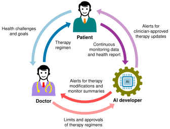](https://mlsysbook.ai/contents/core/ops/2b72f3197e39cf865a675e27089671a8913ffd2e.svg "Figure 11: ClinAIOps Feedback Loops: The cyclical framework coordinates data flow between patients, clinicians, and AI systems to support continuous model improvement and safe clinical integration. These interconnected loops enable iterative refinement of AI models based on real-world performance and clinical feedback, fostering trust and accountability in healthcare applications. Source: [@chen2023framework].")
Figure 11: **ClinAIOps Feedback Loops**: The cyclical framework coordinates data flow between patients, clinicians, and AI systems to support continuous model improvement and safe clinical integration. These interconnected loops enable iterative refinement of AI models based on real-world performance and clinical feedback, fostering trust and accountability in healthcare applications. Source: ([E. Chen et al. 2023](https://mlsysbook.ai/contents/core/ops/ops.html#ref-chen2023framework)
).
In this model, the patient is central: contributing real-world physiological data, reporting outcomes, and serving as the primary beneficiary of optimized care. The clinician interprets this data in context, provides clinical judgment, and oversees treatment adjustments. Meanwhile, the AI system continuously analyzes incoming signals, surfaces actionable insights, and learns from feedback to improve its recommendations.
Each feedback loop plays a distinct yet interconnected role:
* The patient-AI loop captures and interprets real-time physiological data, generating tailored treatment suggestions.
* The Clinician-AI loop ensures that AI-generated recommendations are reviewed, vetted, and refined under professional supervision.
* The Patient-Clinician loop supports shared decision-making, empowering patients and clinicians to collaboratively set goals and interpret data trends.
Together, these loops enable adaptive personalization of care. They help calibrate AI system behavior to the evolving needs of each patient, maintain clinician control over treatment decisions, and promote continuous model improvement based on real-world feedback. By embedding AI within these structured interactions, instead of isolating it as a standalone tool, ClinAIOps provides a blueprint for responsible and effective AI integration into clinical workflows.
##### Patient-AI Loop
The patient–AI loop enables personalized and timely therapy optimization by leveraging continuous physiological data collected through wearable devices. Patients are equipped with sensors such as smartwatches, skin patches, or specialized biosensors that passively capture health-related signals in real-world conditions. For instance, a patient managing diabetes may wear a continuous glucose monitor, while individuals with cardiovascular conditions may use ECG-enabled wearables to track cardiac rhythms.
The AI system continuously analyzes these data streams in conjunction with relevant clinical context drawn from the patient’s electronic medical records, including diagnoses, lab values, prescribed medications, and demographic information. Using this holistic view, the AI model generates individualized recommendations for treatment adjustments, such as modifying dosage levels, altering administration timing, or flagging anomalous trends for review.
To ensure both responsiveness and safety, treatment suggestions are tiered. Minor adjustments that fall within clinician-defined safety thresholds may be acted upon directly by the patient, empowering self-management while reducing clinical burden. More significant changes require review and approval by a healthcare provider. This structure maintains human oversight while enabling high-frequency, data-driven adaptation of therapies.
By enabling real-time, tailored interventions, including automatic insulin dosing adjustments based on glucose trends, this loop exemplifies how machine learning can close the feedback gap between sensing and treatment, allowing for dynamic, context-aware care outside of traditional clinical settings.
##### Clinician-AI Loop
The clinician–AI loop introduces a critical layer of human oversight into the process of AI-assisted therapeutic decision-making. In this loop, the AI system generates treatment recommendations and presents them to the clinician along with concise, interpretable summaries of the underlying patient data. These summaries may include longitudinal trends, sensor-derived metrics, and contextual factors extracted from the electronic health record.
For example, an AI model might recommend a reduction in antihypertensive medication dosage for a patient whose blood pressure has remained consistently below target thresholds. The clinician reviews the recommendation in the context of the patient’s broader clinical profile and may choose to accept, reject, or modify the proposed change. This feedback, in turn, contributes to the continuous refinement of the model, improving its alignment with clinical practice.
Crucially, clinicians also define the operational boundaries within which the AI system can autonomously issue recommendations. These constraints ensure that only low-risk adjustments are automated, while more significant decisions require human approval. This preserves clinical accountability, supports patient safety, and enhances trust in AI-supported workflows.
The clinician–AI loop exemplifies a hybrid model of care in which AI augments rather than replaces human expertise. By enabling efficient review and oversight of algorithmic outputs, it facilitates the integration of machine intelligence into clinical practice while preserving the role of the clinician as the final decision-maker.
##### Patient-Clinician Loop
The patient–clinician loop enhances the quality of clinical interactions by shifting the focus from routine data collection to higher-level interpretation and shared decision-making. With AI systems handling data aggregation and basic trend analysis, clinicians are freed to engage more meaningfully with patients: reviewing patterns, contextualizing insights, and setting personalized health goals.
For example, in managing diabetes, a clinician may use AI-summarized data to guide a discussion on dietary habits and physical activity, tailoring recommendations to the patient’s specific glycemic trends. Rather than adhering to fixed follow-up intervals, visit frequency can be adjusted dynamically based on patient progress and stability, ensuring that care delivery remains responsive and efficient.
This feedback loop positions the clinician not merely as a prescriber but as a coach and advisor, interpreting data through the lens of patient preferences, lifestyle, and clinical judgment. It reinforces the therapeutic alliance by fostering collaboration and mutual understanding, key elements in personalized and patient-centered care.
#### Hypertension Case Example
To concretize the principles of ClinAIOps, consider the management of hypertension, a condition affecting nearly half of adults in the United States (48.1%, or approximately 119.9 million individuals, according to the Centers for Disease Control and Prevention). Effective hypertension control often requires individualized, ongoing adjustments to therapy, making it an ideal candidate for continuous therapeutic monitoring.
ClinAIOps offers a structured framework for managing hypertension by integrating wearable sensing technologies, AI-driven recommendations, and clinician oversight into a cohesive feedback system. In this context, wearable devices equipped with photoplethysmography (PPG) and electrocardiography (ECG) sensors passively capture cardiovascular data, which can be analyzed in near-real-time to inform treatment adjustments. These inputs are augmented by behavioral data (e.g., physical activity) and medication adherence logs, forming the basis for an adaptive and responsive treatment regimen.
The following subsections detail how the patient–AI, clinician–AI, and patient–clinician loops apply in this setting, illustrating the practical implementation of ClinAIOps for a widespread and clinically significant condition.
##### Data Collection
In a ClinAIOps-based hypertension management system, data collection is centered on continuous, multimodal physiological monitoring. Wrist-worn devices equipped with photoplethysmography (PPG)[48](https://mlsysbook.ai/contents/core/ops/ops.html#fn48)
and electrocardiography (ECG) sensors provide noninvasive estimates of blood pressure ([Q. Zhang, Zhou, and Zeng 2017](https://mlsysbook.ai/contents/core/ops/ops.html#ref-zhang2017highly)
). These wearables also include accelerometers to capture physical activity patterns, enabling contextual interpretation of blood pressure fluctuations in relation to movement and exertion.
48 **Photoplethysmography (PPG)**: Optical technique that detects blood volume changes in microvascular tissues by measuring light absorption variations. Invented by Alrick Hertzman in 1936 (though earlier optical pulse detection work existed), who coined the term “photoelectric plethysmograph” while studying blood volume changes in rabbit ears, PPG became the foundation for pulse oximetry in the 1970s. Modern smartwatches use PPG sensors with green LEDs to measure heart rate, with Apple Watch collecting billions of PPG measurements monthly across its user base for heart rhythm analysis and atrial fibrillation detection.
Zhang, Qingxue, Dian Zhou, and Xuan Zeng. 2017. “Highly Wearable Cuff-Less Blood Pressure and Heart Rate Monitoring with Single-Arm Electrocardiogram and Photoplethysmogram Signals.” _BioMedical Engineering OnLine_ 16 (1): 23. [https://doi.org/10.1186/s12938-017-0317-z](https://doi.org/10.1186/s12938-017-0317-z)
.
Complementary data inputs include self-reported logs of antihypertensive medication intake, specifying dosage and timing, as well as demographic attributes and clinical history extracted from the patient’s electronic health record. Together, these heterogeneous data streams form a rich, temporally aligned dataset that captures both physiological states and behavioral factors influencing blood pressure regulation.
By integrating real-world sensor data with longitudinal clinical information, this integrated data foundation enables the development of personalized, context-aware models for adaptive hypertension management.
##### AI Model
The AI component in a ClinAIOps-driven hypertension management system is designed to operate directly on the device or in close proximity to the patient, enabling near real-time analysis and decision support. The model ingests continuous streams of blood pressure estimates, circadian rhythm indicators, physical activity levels, and medication adherence patterns to generate individualized therapeutic recommendations.
Using machine learning techniques, the model infers optimal medication dosing and timing strategies to maintain target blood pressure levels. Minor dosage adjustments that fall within predefined safety thresholds can be communicated directly to the patient, while recommendations involving more substantial modifications are routed to the supervising clinician for review and approval.
The model supports continual refinement through a feedback mechanism that incorporates clinician decisions and patient outcomes. By integrating this observational data into subsequent training iterations, the system incrementally improves its predictive accuracy and clinical utility. The overarching objective is to enable fully personalized, adaptive blood pressure management that evolves in response to each patient’s physiological and behavioral profile.
##### Patient-AI Loop
The patient-AI loop facilitates timely, personalized medication adjustments by delivering AI-generated recommendations directly to the patient through a wearable device or associated mobile application. When the model identifies a minor dosage modification that falls within a pre-approved safety envelope, the patient may act on the suggestion independently, enabling a form of autonomous, yet bounded, therapeutic self-management.
For recommendations involving significant changes to the prescribed regimen, the system defers to clinician oversight, ensuring medical accountability and compliance with regulatory standards. This loop empowers patients to engage actively in their care while maintaining a safeguard for clinical appropriateness.
By enabling personalized, data-driven feedback on a daily basis, the patient-AI loop supports improved adherence and therapeutic outcomes. It operationalizes a key principle of ClinAIOps, by closing the loop between continuous monitoring and adaptive intervention, while preserving the patient’s role as an active agent in the treatment process.
##### Clinician-AI Loop
The clinician-AI loop ensures medical oversight by placing healthcare providers at the center of the decision-making process. Clinicians receive structured summaries of the patient’s longitudinal blood pressure patterns, visualizations of adherence behaviors, and relevant contextual data aggregated from wearable sensors and electronic health records. These insights support efficient and informed review of the AI system’s recommended medication adjustments.
Before reaching the patient, the clinician evaluates each proposed dosage change, choosing to approve, modify, or reject the recommendation based on their professional judgment and understanding of the patient’s broader clinical profile. Clinicians define the operational boundaries within which the AI may act autonomously, specifying thresholds for dosage changes that can be enacted without direct review.
When the system detects blood pressure trends indicative of clinical risk, including persistent hypotension or a hypertensive crisis, it generates alerts for immediate clinician intervention. These capabilities preserve the clinician’s authority over treatment while enhancing their ability to manage patient care proactively and at scale.
This loop exemplifies the principles of accountability, safety, and human-in-the-loop governance, ensuring that AI functions as a supportive tool rather than an autonomous agent in therapeutic decision-making.
##### Patient-Clinician Loop
As illustrated in [Figure 12](https://mlsysbook.ai/contents/core/ops/ops.html#fig-interactive-loop)
, the patient-clinician loop emphasizes collaboration, context, and continuity in care. Rather than devoting in-person visits to basic data collection or medication reconciliation, clinicians engage with patients to interpret high-level trends derived from continuous monitoring. These discussions focus on modifiable factors such as diet, physical activity, sleep quality, and stress management, enabling a more holistic approach to blood pressure control.
[](https://mlsysbook.ai/contents/core/ops/152459d2567c0229fa3bd608f063eb3b8c21562b.svg "Figure 12: Patient-Clinician Interaction: Continuous monitoring data informs collaborative discussions between patients and clinicians, shifting focus from data collection to actionable insights for lifestyle modifications and improved health management. This loop prioritizes patient engagement and contextual understanding to facilitate personalized care beyond traditional clinical visits. Source: [@chen2023framework].")
Figure 12: **Patient-Clinician Interaction**: Continuous monitoring data informs collaborative discussions between patients and clinicians, shifting focus from data collection to actionable insights for lifestyle modifications and improved health management. This loop prioritizes patient engagement and contextual understanding to facilitate personalized care beyond traditional clinical visits. Source: ([E. Chen et al. 2023](https://mlsysbook.ai/contents/core/ops/ops.html#ref-chen2023framework)
).
Chen, Emma, Shvetank Prakash, Vijay Janapa Reddi, David Kim, and Pranav Rajpurkar. 2023. “A Framework for Integrating Artificial Intelligence for Clinical Care with Continuous Therapeutic Monitoring.” _Nature Biomedical Engineering_ 9 (4): 445–54. [https://doi.org/10.1038/s41551-023-01115-0](https://doi.org/10.1038/s41551-023-01115-0)
.
The dynamic nature of continuous data allows for flexible scheduling of appointments based on clinical need rather than fixed intervals. For example, patients exhibiting stable blood pressure trends may be seen less frequently, while those experiencing variability may receive more immediate follow-up. This adaptive cadence enhances resource efficiency while preserving care quality.
By offloading routine monitoring and dose titration to AI-assisted systems, clinicians are better positioned to offer personalized counseling and targeted interventions. The result is a more meaningful patient-clinician relationship that supports shared decision-making and long-term wellness. This loop exemplifies how ClinAIOps frameworks can shift clinical interactions from transactional to transformational, supporting proactive care, patient empowerment, and improved health outcomes.
#### MLOps vs ClinAIOps Comparison
The hypertension case study illustrates why traditional MLOps frameworks are often insufficient for high-stakes, real-world domains such as clinical healthcare. While conventional MLOps excels at managing the technical lifecycle of machine learning models, including training, deployment, and monitoring, it generally lacks the constructs necessary for coordinating human decision-making, managing clinical workflows, and safeguarding ethical accountability.
In contrast, the ClinAIOps framework extends beyond technical infrastructure to support complex sociotechnical systems. Rather than treating the model as the final decision-maker, ClinAIOps embeds machine learning into a broader context where clinicians, patients, and systems stakeholders collaboratively shape treatment decisions.
Several limitations of a traditional MLOps approach become apparent when applied to a clinical setting like hypertension management:
* **Data availability and feedback**: Traditional pipelines rely on pre-collected datasets. ClinAIOps enables ongoing data acquisition and iterative feedback from clinicians and patients.
* **Trust and interpretability**: MLOps may lack transparency mechanisms for end users. ClinAIOps maintains clinician oversight, ensuring recommendations remain actionable and trustworthy.
* **Behavioral and motivational factors**: MLOps focuses on model outputs. ClinAIOps recognizes the need for patient coaching, adherence support, and personalized engagement.
* **Safety and liability**: MLOps does not account for medical risk. ClinAIOps retains human accountability and provides structured boundaries for autonomous decisions.
* **Workflow integration**: Traditional systems may exist in silos. ClinAIOps aligns incentives and communication across stakeholders to ensure clinical adoption.
As shown in [Table 7](https://mlsysbook.ai/contents/core/ops/ops.html#tbl-clinical_ops)
, the key distinction lies in how ClinAIOps integrates technical systems with human oversight, ethical principles, and care delivery processes. Rather than replacing clinicians, the framework augments their capabilities while preserving their central role in therapeutic decision-making.
Table 7: **Clinical AI Operations**: Traditional MLOps focuses on model performance, while ClinAIOps integrates technical systems with clinical workflows, ethical considerations, and ongoing feedback loops to ensure safe, trustworthy, and effective AI assistance in healthcare settings. This table emphasizes that ClinAIOps prioritizes human oversight and accountability alongside automation, addressing unique challenges in clinical decision-making that standard MLOps pipelines often overlook.
| | | |
| --- | --- | --- |
| **Focus** | ML model development and deployment | Coordinating human and AI decision-making |
| **Stakeholders** | Data scientists, IT engineers | Patients, clinicians, AI developers |
| **Feedback loops** | Model retraining, monitoring | Patient-AI, clinician-AI, patient-clinician |
| **Objective** | Operationalize ML deployments | Optimize patient health outcomes |
| **Processes** | Automated pipelines and infrastructure | Integrates clinical workflows and oversight |
| **Data considerations** | Building training datasets | Privacy, ethics, protected health information |
| **Model validation** | Testing model performance metrics | Clinical evaluation of recommendations |
| **Implementation** | Focuses on technical integration | Aligns incentives of human stakeholders |
Successfully deploying AI in complex domains such as healthcare requires more than developing and operationalizing performant machine learning models. As demonstrated by the hypertension case, effective integration depends on aligning AI systems with clinical workflows, human expertise, and patient needs. Technical performance alone is insufficient; deployment must account for ethical oversight, stakeholder coordination, and continuous adaptation to dynamic clinical contexts.
The ClinAIOps framework specifically addresses the operational challenges identified earlier, demonstrating how they manifest in healthcare contexts. Rather than treating feedback loops as technical debt, ClinAIOps explicitly architects them as beneficial system features, with patient-AI, clinician-AI, and patient-clinician loops creating intentional feedback mechanisms that improve care quality while maintaining safety through human oversight. The structured interface between AI recommendations and clinical decision-making eliminates hidden dependencies, ensuring clinicians maintain explicit control over AI outputs and preventing the silent breakage that occurs when model updates unexpectedly affect downstream systems. Clear delineation of AI responsibilities for monitoring and recommendations versus human responsibilities for diagnosis and treatment decisions prevents the gradual erosion of system boundaries that undermines reliability in complex ML systems. The framework’s emphasis on regulatory compliance, ethical oversight, and clinical validation creates systematic approaches to configuration management that prevent the ad hoc practices accumulating governance debt in healthcare AI systems. By embedding AI within collaborative clinical ecosystems, ClinAIOps demonstrates how operational challenges can be transformed from liabilities into systematic design opportunities, reframing AI not as an isolated technical artifact but as a component of a broader sociotechnical system designed to advance health outcomes while maintaining the engineering rigor essential for production ML systems.
**Self-Check: Question 1.8**
1. In the Oura Ring case study, which operational challenge is primarily addressed by the implementation of automated data pipelines?
1. Feedback loop management
2. Role specialization
3. Configuration debt
4. Data dependency debt
2. Explain how the ClinAIOps framework adapts traditional MLOps practices to meet the needs of clinical environments.
3. The Oura Ring’s transition from a 62% to a clinical-grade accuracy in classifying sleep stages was achieved by addressing \_\_\_\_, which involves managing fragmented settings in embedded ML deployments.
4. Order the following steps in the Oura Ring’s model deployment process: (1) Model compression, (2) OTA updates, (3) Model validation, (4) Deployment to embedded hardware.
[See Answers →](https://mlsysbook.ai/contents/core/ops/ops.html#quiz-answer-sec-ml-operations-case-studies-1206)
Fallacies and Pitfalls
----------------------
Machine learning operations introduces unique complexities that distinguish it from traditional software deployment, yet many teams underestimate these differences and attempt to apply conventional practices without adaptation. The probabilistic nature of ML systems, the central role of data quality, and the need for continuous model maintenance create operational challenges that require specialized approaches and tooling.
**Fallacy:** _MLOps is just applying traditional DevOps practices to machine learning models._
This misconception leads teams to apply conventional software deployment practices to ML systems without understanding their unique characteristics. Traditional software has deterministic behavior and clear input-output relationships, while ML systems exhibit probabilistic behavior, data dependencies, and model drift. Standard CI/CD pipelines fail to account for data validation, model performance monitoring, or retraining triggers that are essential for ML systems. Feature stores, model registries, and drift detection require specialized infrastructure not present in traditional DevOps. Effective MLOps requires dedicated practices designed for the stochastic and data-dependent nature of machine learning systems.
**Pitfall:** _Treating model deployment as a one-time event rather than an ongoing process._
Many teams view model deployment as the final step in the ML lifecycle, similar to shipping software releases. This approach ignores the reality that ML models degrade over time due to data drift, changing user behavior, and evolving business requirements. Production models require continuous monitoring, performance evaluation, and potential retraining or replacement. Without ongoing operational support, deployed models become unreliable and may produce increasingly poor results. Successful MLOps treats deployment as the beginning of a model’s operational lifecycle rather than its conclusion.
**Fallacy:** _Automated retraining ensures optimal model performance without human oversight._
This belief assumes that automated pipelines can handle all aspects of model maintenance without human intervention. While automation is essential for scalable MLOps, it cannot handle all scenarios that arise in production. Automated retraining might perpetuate biases present in new training data, fail to detect subtle quality issues, or trigger updates during inappropriate times. Complex failure modes, regulatory requirements, and business logic changes require human judgment and oversight. Effective MLOps balances automation with appropriate human checkpoints and intervention capabilities.
**Pitfall:** _Focusing on technical infrastructure while neglecting organizational and process alignment._
Organizations often invest heavily in MLOps tooling and platforms without addressing the cultural and process changes required for successful implementation. MLOps requires close collaboration between data scientists, engineers, and business stakeholders with different backgrounds, priorities, and communication styles. Without clear roles, responsibilities, and communication protocols, sophisticated technical infrastructure fails to deliver operational benefits. Successful MLOps implementation requires organizational transformation that aligns incentives, establishes shared metrics, and creates collaborative workflows across functional boundaries.
**Self-Check: Question 1.9**
1. Which of the following best describes a key difference between traditional DevOps and MLOps?
1. Traditional DevOps focuses on deterministic software behavior, while MLOps manages probabilistic models.
2. MLOps requires less infrastructure than traditional DevOps.
3. Traditional DevOps does not involve any form of automation.
4. MLOps completely eliminates the need for human oversight.
2. True or False: Automated retraining pipelines in MLOps can fully replace human oversight.
3. Why is ongoing model maintenance critical in MLOps, and what are the potential consequences of neglecting it?
4. In MLOps, the concept of treating model deployment as a(n) \_\_\_\_ rather than a one-time event is crucial.
5. Consider a scenario where an e-commerce company is deploying a recommendation system. What organizational changes might be necessary to support effective MLOps implementation?
[See Answers →](https://mlsysbook.ai/contents/core/ops/ops.html#quiz-answer-sec-ml-operations-fallacies-pitfalls-0381)
Summary
-------
Machine learning operations provides the comprehensive framework that integrates the specialized capabilities explored throughout this book into cohesive production systems. The preceding chapters established critical operational requirements: **[Chapter 14: On-Device Learning](https://mlsysbook.ai/contents/core/ondevice_learning/ondevice_learning.html#sec-ondevice-learning)
** demonstrated federated learning and edge adaptation under severe constraints, **[Chapter 15: Security & Privacy](https://mlsysbook.ai/contents/core/privacy_security/privacy_security.html#sec-security-privacy)
** developed privacy-preserving techniques and secure model serving, and **[Chapter 16: Robust AI](https://mlsysbook.ai/contents/core/robust_ai/robust_ai.html#sec-robust-ai)
** presented fault tolerance mechanisms for unpredictable environments. This chapter revealed how MLOps orchestrates these diverse capabilities through systematic engineering practices—data pipeline automation, model versioning, infrastructure orchestration, and continuous monitoring—that enable edge learning, security controls, and robustness mechanisms to function together reliably at scale. The evolution from isolated technical solutions to integrated operational frameworks reflects the maturity of ML systems engineering as a discipline capable of delivering sustained value in production environments.
The operational challenges of machine learning systems span technical, organizational, and domain-specific dimensions that require sophisticated coordination across multiple stakeholders and system components. Data drift detection and model retraining pipelines must operate continuously to maintain system performance as real-world conditions change. Infrastructure automation enables reproducible deployments across diverse environments while version control systems track the complex relationships between code, data, and model artifacts. The monitoring frameworks discussed earlier must capture both traditional system metrics and ML-specific indicators like prediction confidence, feature distribution shifts, and model fairness metrics. The integration of these operational capabilities creates robust feedback loops that enable systems to adapt to changing conditions while maintaining reliability and performance guarantees.
Key Takeaways
* MLOps provides the comprehensive framework integrating specialized capabilities from edge learning (**[Chapter 14: On-Device Learning](https://mlsysbook.ai/contents/core/ondevice_learning/ondevice_learning.html#sec-ondevice-learning)
**), security (**[Chapter 15: Security & Privacy](https://mlsysbook.ai/contents/core/privacy_security/privacy_security.html#sec-security-privacy)
**), and robustness (**[Chapter 16: Robust AI](https://mlsysbook.ai/contents/core/robust_ai/robust_ai.html#sec-robust-ai)
**) into cohesive production systems
* Technical debt patterns like feedback loops and data dependencies require systematic engineering solutions through feature stores, versioning systems, and monitoring frameworks
* Infrastructure components directly address operational challenges: CI/CD pipelines prevent correction cascades, model registries enable controlled rollbacks, and orchestration tools manage distributed deployments
* Production operations must simultaneously handle federated edge updates, maintain privacy guarantees, and detect adversarial degradation through unified monitoring and governance
* Domain-specific frameworks like ClinAIOps transform operational challenges into design opportunities, showing how MLOps adapts to specialized requirements while maintaining engineering rigor
The MLOps framework presented in this chapter represents the culmination of the specialized capabilities developed throughout Part IV. The edge learning techniques from **[Chapter 14: On-Device Learning](https://mlsysbook.ai/contents/core/ondevice_learning/ondevice_learning.html#sec-ondevice-learning)
** require MLOps adaptations for distributed model updates without centralized visibility. The security mechanisms from **[Chapter 15: Security & Privacy](https://mlsysbook.ai/contents/core/privacy_security/privacy_security.html#sec-security-privacy)
** depend on MLOps infrastructure for secure model deployment and privacy-preserving training pipelines. The robustness strategies from **[Chapter 16: Robust AI](https://mlsysbook.ai/contents/core/robust_ai/robust_ai.html#sec-robust-ai)
** rely on MLOps monitoring to detect distribution shifts and trigger appropriate mitigations. As machine learning systems mature from experimental prototypes to production services, MLOps provides the essential engineering discipline that enables these specialized capabilities to work together reliably. The operational excellence principles developed through MLOps practice ensure that AI systems remain trustworthy, maintainable, and effective in addressing real-world challenges at scale, transforming the promise of machine learning into sustained operational value.
**Self-Check: Question 1.10**
1. Which of the following best describes the role of MLOps in integrating specialized capabilities into production systems?
1. MLOps focuses solely on model training.
2. MLOps only deals with model deployment.
3. MLOps is primarily concerned with data collection.
4. MLOps integrates edge learning, security, and robustness into cohesive systems.
2. Explain how MLOps addresses the operational challenges of data drift detection and model retraining in production systems.
3. Order the following MLOps components based on their role in maintaining system reliability: (1) Model versioning, (2) Continuous monitoring, (3) Infrastructure automation.
4. What operational challenge is addressed by implementing unified monitoring and governance in MLOps?
1. Reducing training time
2. Detecting adversarial degradation
3. Simplifying data collection
4. Improving user interface design
[See Answers →](https://mlsysbook.ai/contents/core/ops/ops.html#quiz-answer-sec-ml-operations-summary-5a7c)
Self-Check Answers
------------------
**Self-Check: Answer 1.1**
1. **What is the Silent Failure Problem in machine learning systems?**
1. A sudden crash of the system with error messages.
2. Gradual performance degradation without noticeable alerts.
3. A complete failure of the model to make predictions.
4. An increase in computational resource usage.
_Answer_: The correct answer is B. Gradual performance degradation without noticeable alerts. This is correct because silent failures occur as data distributions shift and model assumptions become outdated, leading to performance issues without explicit errors.
_Learning Objective_: Understand the concept of silent failures in ML systems.
2. **How does MLOps address the Silent Failure Problem in machine learning systems?**
_Answer_: MLOps addresses the Silent Failure Problem by implementing monitoring, automation, and governance to detect and manage performance degradation. For example, it enables continuous model retraining and real-time performance assessment. This is important because it ensures that models remain reliable and performant in production environments.
_Learning Objective_: Explain how MLOps helps in managing silent failures in ML systems.
3. **Which of the following best describes the role of MLOps in machine learning system deployment?**
1. It provides a framework for automated, end-to-end lifecycle management.
2. It focuses solely on algorithmic innovation.
3. It is concerned only with the security of machine learning models.
4. It replaces the need for data science practices.
_Answer_: The correct answer is A. It provides a framework for automated, end-to-end lifecycle management. This is correct because MLOps integrates methodologies from machine learning, data science, and software engineering to manage the entire lifecycle of ML systems.
_Learning Objective_: Identify the role of MLOps in the deployment of ML systems.
4. **Consider a scenario where a ridesharing service is deploying a demand prediction system. What are some operational challenges that MLOps can help address in this context?**
_Answer_: MLOps can help address challenges such as varying data quality, seasonal changes in temporal patterns, and the need for real-time response capabilities. For example, it supports continuous model retraining and evaluation against production baselines. This is important because it ensures the system meets strict availability and performance requirements.
_Learning Objective_: Apply MLOps concepts to real-world ML system deployment challenges.
[← Back to Questions](https://mlsysbook.ai/contents/core/ops/ops.html#quiz-question-sec-ml-operations-introduction-machine-learning-operations-5f4b)
**Self-Check: Answer 1.2**
1. **What was the primary motivation for the evolution from DevOps to MLOps?**
1. To address the unique complexities of machine learning workflows
2. To improve software deployment speeds
3. To enhance collaboration between developers and IT operations
4. To reduce costs in software development
_Answer_: The correct answer is A. To address the unique complexities of machine learning workflows. MLOps evolved from DevOps to manage non-deterministic, data-dependent workflows specific to ML systems.
_Learning Objective_: Understand the primary motivations behind the transition from DevOps to MLOps.
2. **Explain how the concept of ‘Infrastructure as Code’ contributed to the development of DevOps practices.**
_Answer_: Infrastructure as Code allowed for the automation and reproducibility of infrastructure setups, reducing manual errors and enabling rapid deployment. This concept was crucial in addressing inefficiencies in traditional software pipelines and laid the groundwork for DevOps by promoting shared ownership and streamlined deployment processes.
_Learning Objective_: Analyze the role of ‘Infrastructure as Code’ in the development of DevOps practices.
3. **Which of the following is a key difference between DevOps and MLOps?**
1. DevOps and MLOps both focus on data versioning.
2. DevOps emphasizes model versioning, whereas MLOps does not.
3. DevOps focuses on deterministic software, while MLOps manages non-deterministic workflows.
4. MLOps is primarily concerned with software release management.
_Answer_: The correct answer is C. DevOps focuses on deterministic software, while MLOps manages non-deterministic workflows. MLOps addresses the unique challenges of ML systems, such as data and model versioning.
_Learning Objective_: Identify key differences between DevOps and MLOps.
4. **In a production system, how might MLOps practices prevent issues like the silent data drift problem described in the section?**
_Answer_: MLOps practices include continuous monitoring of model performance and automated retraining, which can detect and address data drift issues before they degrade model accuracy. By implementing these practices, organizations can maintain model reliability and prevent significant business impacts.
_Learning Objective_: Apply MLOps practices to prevent and manage data drift issues in production systems.
[← Back to Questions](https://mlsysbook.ai/contents/core/ops/ops.html#quiz-question-sec-ml-operations-historical-context-8f3a)
**Self-Check: Answer 1.3**
1. **What is a primary cause of boundary erosion in machine learning systems?**
1. Explicit interfaces between components
2. Strong modularity and encapsulation
3. Statistical rather than logical guarantees
4. Comprehensive testing and validation
_Answer_: The correct answer is C. Statistical rather than logical guarantees. This is correct because ML systems operate with statistical dependencies which blur boundaries, unlike traditional software with logical guarantees. Options A, B, and D represent solutions to boundary erosion rather than causes.
_Learning Objective_: Understand the causes of boundary erosion in ML systems.
2. **Explain how correction cascades can affect the lifecycle of a machine learning system.**
_Answer_: Correction cascades occur when small adjustments in ML systems trigger dependent fixes across the workflow, leading to widespread changes. For example, modifying a model may require updates in data preprocessing, affecting downstream systems. This is important because it highlights the need for modular design to prevent such cascading effects.
_Learning Objective_: Analyze the impact of correction cascades on ML system lifecycle.
3. **Which of the following best describes the CACHE principle in ML systems?**
1. A method to cache intermediate results to improve efficiency
2. A principle for optimizing computational resources
3. A strategy for efficient data storage and retrieval
4. A phenomenon where any change can affect the entire system
_Answer_: The correct answer is D. A phenomenon where any change can affect the entire system. This is correct because CACHE represents the risk of widespread impact from local changes due to weak boundaries in ML systems. Options A, B, and C do not relate to the concept of boundary erosion.
_Learning Objective_: Understand the implications of the CACHE principle in ML systems.
4. **Order the following stages to illustrate the propagation of correction cascades in an ML system: (1) Model training, (2) Data collection, (3) Model deployment, (4) Model evaluation.**
_Answer_: The correct order is: (2) Data collection, (1) Model training, (4) Model evaluation, (3) Model deployment. Correction cascades typically start with data collection, followed by model training, evaluation, and finally deployment. Understanding this order helps in anticipating and mitigating cascading effects.
_Learning Objective_: Reinforce understanding of the sequence and impact of correction cascades in ML systems.
5. **In a production system, how might you address undeclared consumer debt to improve system reliability?**
_Answer_: Addressing undeclared consumer debt involves implementing strict access controls for model outputs and formalizing interface contracts with documented schemas. For example, ensuring that all model outputs are tracked and documented prevents silent failures when models evolve. This is important because it enhances system reliability by reducing hidden dependencies.
_Learning Objective_: Apply solutions to manage undeclared consumer debt in ML systems.
[← Back to Questions](https://mlsysbook.ai/contents/core/ops/ops.html#quiz-question-sec-ml-operations-technical-debt-system-complexity-0bb6)
**Self-Check: Answer 1.4**
1. **Which of the following best describes the role of feature stores in MLOps infrastructure?**
1. They store raw data for model training.
2. They serve as repositories for model versioning.
3. They provide cloud storage solutions for data artifacts.
4. They manage engineered features for consistent access across training and inference.
_Answer_: The correct answer is D. They manage engineered features for consistent access across training and inference. Feature stores ensure that features are consistently available and versioned, reducing risks of training-serving skew.
_Learning Objective_: Understand the function and importance of feature stores in MLOps.
2. **How does the integration of CI/CD pipelines enhance the reliability and reproducibility of machine learning models in production?**
_Answer_: CI/CD pipelines automate the ML lifecycle, ensuring that model updates are systematically tested, validated, and deployed. They reduce manual errors, enforce quality checks, and support continuous improvement, thereby enhancing reliability and reproducibility. For example, a CI/CD pipeline can automatically trigger retraining when data drift is detected, ensuring models remain accurate over time.
_Learning Objective_: Explain the benefits of CI/CD pipelines in maintaining model reliability and reproducibility.
3. **Order the following MLOps infrastructure components from data ingestion to model deployment: (1) Data Management, (2) Model Training, (3) Feature Store, (4) Model Serving.**
_Answer_: The correct order is: (1) Data Management, (3) Feature Store, (2) Model Training, (4) Model Serving. Data is first managed and preprocessed, features are stored for consistency, models are trained using these features, and finally, models are served for inference.
_Learning Objective_: Understand the sequence of MLOps components from data handling to model deployment.
4. **True or False: In MLOps, the primary purpose of data versioning is to ensure that model training can be reproduced exactly at any point in the future.**
_Answer_: True. This is true because data versioning allows teams to snapshot datasets and associate them with specific model runs, ensuring reproducibility and traceability across the ML lifecycle.
_Learning Objective_: Recognize the importance of data versioning in reproducibility and traceability.
5. **Consider a scenario where an industrial predictive maintenance system is deployed. What role does a feature store play in ensuring the system’s operational efficiency?**
_Answer_: In a predictive maintenance system, a feature store centralizes and manages the features derived from sensor data and historical logs, ensuring consistency across training and inference. This reduces duplication of feature engineering efforts and minimizes risks of training-serving skew, thereby maintaining operational efficiency. For example, by storing rolling averages and statistical aggregates in a feature store, the system can quickly access and update these features for real-time predictions.
_Learning Objective_: Apply the concept of feature stores to real-world MLOps scenarios to ensure consistent and efficient model operations.
[← Back to Questions](https://mlsysbook.ai/contents/core/ops/ops.html#quiz-question-sec-ml-operations-development-infrastructure-automation-0be4)
**Self-Check: Answer 1.5**
1. **Which deployment strategy involves maintaining two identical production environments to enable zero-downtime updates?**
1. Canary Deployment
2. Blue-Green Deployment
3. Shadow Deployment
4. Rolling Deployment
_Answer_: The correct answer is B. Blue-Green Deployment. This strategy involves maintaining two identical environments, one serving traffic while the other is updated, allowing instant traffic switch to minimize downtime. Canary Deployment and Shadow Deployment are incremental and testing strategies, respectively.
_Learning Objective_: Understand different deployment strategies and their operational implications.
2. **Explain how model orchestration can enhance the efficiency of serving large-scale machine learning models.**
_Answer_: Model orchestration coordinates the execution of multi-stage models or distributed components, optimizing resource allocation and enabling parallel processing. For example, AlpaServe orchestrates large models by managing resources efficiently, which is crucial for handling complex serving scenarios. This is important because it improves throughput and reduces latency, meeting performance targets in production environments.
_Learning Objective_: Analyze the role of model orchestration in improving serving efficiency for large-scale ML models.
3. **True or False: Inference endpoints typically expose deployed models via REST APIs for real-time predictions.**
_Answer_: True. This is true because inference endpoints are designed to make models accessible for real-time predictions, often using REST APIs to handle inference requests efficiently.
_Learning Objective_: Recognize the role of inference endpoints in serving infrastructure.
4. **What is a primary benefit of using model registries in production ML systems?**
1. They eliminate the need for model testing.
2. They ensure models are always up-to-date without human intervention.
3. They automatically improve model accuracy.
4. They provide a centralized repository for managing model versions and metadata.
_Answer_: The correct answer is D. They provide a centralized repository for managing model versions and metadata. Model registries facilitate version tracking and comparison, which is essential for maintaining model lineage and auditability. Options A, B, and C are incorrect because model registries do not inherently perform those functions.
_Learning Objective_: Understand the role and benefits of model registries in managing production ML systems.
5. **In a production system, how might you apply governance frameworks to ensure model compliance with ethical and regulatory standards?**
_Answer_: Governance frameworks ensure compliance by implementing policies for transparency, fairness, and accountability. For example, using tools like SHAP for interpretability and bias detection ensures models are fair and compliant with regulations. This is important because it mitigates legal and reputational risks, ensuring models serve societal goals responsibly.
_Learning Objective_: Apply governance frameworks to ensure ethical and regulatory compliance in ML systems.
[← Back to Questions](https://mlsysbook.ai/contents/core/ops/ops.html#quiz-question-sec-ml-operations-production-operations-a18c)
**Self-Check: Answer 1.6**
1. **Which role is primarily responsible for ensuring data quality and managing data pipelines in an MLOps framework?**
1. Data Scientist
2. ML Engineer
3. DevOps Engineer
4. Data Engineer
_Answer_: The correct answer is D. Data Engineer. Data Engineers are responsible for building and maintaining data pipelines, ensuring data quality, and managing data infrastructure. Data Scientists focus on model development, while ML Engineers handle model deployment and integration.
_Learning Objective_: Understand the primary responsibilities of a Data Engineer in MLOps.
2. **Explain how the handoff between Data Scientists and ML Engineers is critical for successful model deployment in MLOps.**
_Answer_: The handoff between Data Scientists and ML Engineers involves transitioning models from research to production. ML Engineers must understand model requirements to optimize performance and integrate them into applications. This step ensures that models are robust, scalable, and meet production constraints, reducing errors and improving deployment efficiency.
_Learning Objective_: Analyze the importance of role handoffs in the MLOps lifecycle.
3. **True or False: In an MLOps framework, DevOps Engineers are primarily responsible for model development and experimentation.**
_Answer_: False. DevOps Engineers focus on infrastructure orchestration, automation, and monitoring, not model development. Data Scientists handle model development and experimentation.
_Learning Objective_: Differentiate between the roles of DevOps Engineers and Data Scientists in MLOps.
4. **Order the following roles based on their typical involvement in the MLOps lifecycle from data preparation to deployment: (1) Data Engineer, (2) ML Engineer, (3) Data Scientist, (4) DevOps Engineer.**
_Answer_: The correct order is: (1) Data Engineer, (3) Data Scientist, (2) ML Engineer, (4) DevOps Engineer. Data Engineers prepare data, Data Scientists develop models, ML Engineers deploy models, and DevOps Engineers manage infrastructure and monitoring.
_Learning Objective_: Understand the sequential involvement of different roles in the MLOps lifecycle.
[← Back to Questions](https://mlsysbook.ai/contents/core/ops/ops.html#quiz-question-sec-ml-operations-roles-responsibilities-79d5)
**Self-Check: Answer 1.7**
1. **What is a key characteristic of high operational maturity in ML systems?**
1. Manual data processing and local training
2. Ad hoc experimentation and unclear ownership
3. Hand-crafted scripts for deployment
4. Automated workflows and integrated observability
_Answer_: The correct answer is D. Automated workflows and integrated observability. High operational maturity involves fully automated workflows, integrated observability, and infrastructure-as-code, supporting reliability and scalability.
_Learning Objective_: Understand the characteristics of high operational maturity in ML systems.
2. **Explain how operational maturity influences the design of ML system architecture.**
_Answer_: Operational maturity influences ML system architecture by requiring modularity, automation, and monitoring. As maturity increases, systems evolve from monolithic scripts to modular abstractions with APIs and orchestration frameworks, supporting scalability and maintainability. This is important because it allows systems to adapt to changing requirements and maintain performance over time.
_Learning Objective_: Analyze how operational maturity impacts ML system architecture design.
3. **True or False: Operational maturity in ML systems is solely determined by the adoption of specific tools such as CI/CD pipelines.**
_Answer_: False. Operational maturity is not solely determined by tool adoption; it centers on system integration and coordination among teams, processes, and technologies.
_Learning Objective_: Challenge the misconception that operational maturity is only about tool adoption.
4. **In high-maturity ML environments, system behavior is monitored in real time and adapted as needed, enabling \_\_\_\_\_\_ development.**
_Answer_: feedback-driven. Feedback-driven development allows systems to respond to real-time data and operational conditions, supporting continuous improvement and adaptation.
_Learning Objective_: Recall the concept of feedback-driven development in high-maturity ML environments.
5. **In a production system, how might the concept of operational maturity guide the prioritization of investments in MLOps infrastructure?**
_Answer_: Operational maturity guides investment prioritization by identifying which practices support scalability, reliability, and observability. Investments should focus on automating workflows, integrating observability, and ensuring governance, as these elements reduce operational friction and support robust decision-making. This is important because it aligns resource allocation with long-term system sustainability.
_Learning Objective_: Apply the concept of operational maturity to prioritize investments in MLOps infrastructure.
[← Back to Questions](https://mlsysbook.ai/contents/core/ops/ops.html#quiz-question-sec-ml-operations-system-design-maturity-framework-d137)
**Self-Check: Answer 1.8**
1. **In the Oura Ring case study, which operational challenge is primarily addressed by the implementation of automated data pipelines?**
1. Feedback loop management
2. Role specialization
3. Configuration debt
4. Data dependency debt
_Answer_: The correct answer is D. Data dependency debt. Automated data pipelines help manage and mitigate data dependency debt by ensuring data consistency and integrity across different stages of the ML lifecycle.
_Learning Objective_: Understand how automated data pipelines address data dependency debt in embedded systems.
2. **Explain how the ClinAIOps framework adapts traditional MLOps practices to meet the needs of clinical environments.**
_Answer_: ClinAIOps adapts traditional MLOps by integrating human oversight, ethical governance, and clinical validation into AI operations. It emphasizes feedback loops between patients, clinicians, and AI systems to ensure safe and effective AI integration into clinical workflows. This approach addresses the unique regulatory and ethical challenges of healthcare, ensuring AI systems support rather than replace human decision-making.
_Learning Objective_: Analyze how ClinAIOps modifies MLOps practices for healthcare applications.
3. **The Oura Ring’s transition from a 62% to a clinical-grade accuracy in classifying sleep stages was achieved by addressing \_\_\_\_, which involves managing fragmented settings in embedded ML deployments.**
_Answer_: configuration debt. Configuration debt involves managing fragmented settings in embedded ML deployments, which can undermine performance and reliability.
_Learning Objective_: Identify the role of configuration management in improving model accuracy.
4. **Order the following steps in the Oura Ring’s model deployment process: (1) Model compression, (2) OTA updates, (3) Model validation, (4) Deployment to embedded hardware.**
_Answer_: The correct order is: (3) Model validation, (1) Model compression, (4) Deployment to embedded hardware, (2) OTA updates. Model validation ensures accuracy, compression optimizes for resource constraints, deployment places models on devices, and OTA updates maintain consistency.
_Learning Objective_: Understand the sequence of steps in deploying ML models to embedded systems.
[← Back to Questions](https://mlsysbook.ai/contents/core/ops/ops.html#quiz-question-sec-ml-operations-case-studies-1206)
**Self-Check: Answer 1.9**
1. **Which of the following best describes a key difference between traditional DevOps and MLOps?**
1. Traditional DevOps focuses on deterministic software behavior, while MLOps manages probabilistic models.
2. MLOps requires less infrastructure than traditional DevOps.
3. Traditional DevOps does not involve any form of automation.
4. MLOps completely eliminates the need for human oversight.
_Answer_: The correct answer is A. Traditional DevOps focuses on deterministic software behavior, while MLOps manages probabilistic models. This is correct because ML systems exhibit probabilistic behavior and require specialized approaches. Options B, C, and D are incorrect because MLOps often requires more infrastructure, involves automation, and still needs human oversight.
_Learning Objective_: Understand the fundamental differences between DevOps and MLOps.
2. **True or False: Automated retraining pipelines in MLOps can fully replace human oversight.**
_Answer_: False. This is false because while automation is crucial for scalability, it cannot handle all scenarios, such as biases in new data or regulatory requirements, which require human judgment.
_Learning Objective_: Recognize the limitations of automation in MLOps.
3. **Why is ongoing model maintenance critical in MLOps, and what are the potential consequences of neglecting it?**
_Answer_: Ongoing model maintenance is critical because ML models degrade over time due to data drift and changing user behavior. Neglecting maintenance can lead to unreliable models and poor results. For example, a model trained on outdated data may fail to predict current trends. This is important because continuous monitoring and retraining ensure model relevance and accuracy.
_Learning Objective_: Explain the importance of continuous model maintenance in MLOps.
4. **In MLOps, the concept of treating model deployment as a(n) \_\_\_\_ rather than a one-time event is crucial.**
_Answer_: ongoing process. This approach acknowledges that models need continuous monitoring and updates to remain effective.
_Learning Objective_: Understand the lifecycle approach to model deployment in MLOps.
5. **Consider a scenario where an e-commerce company is deploying a recommendation system. What organizational changes might be necessary to support effective MLOps implementation?**
_Answer_: To support effective MLOps, the company needs to align data scientists, engineers, and business stakeholders with clear roles and communication protocols. For example, establishing shared metrics and collaborative workflows can enhance operational benefits. This is important because technical infrastructure alone cannot ensure successful MLOps without organizational alignment.
_Learning Objective_: Identify organizational changes needed for successful MLOps implementation.
[← Back to Questions](https://mlsysbook.ai/contents/core/ops/ops.html#quiz-question-sec-ml-operations-fallacies-pitfalls-0381)
**Self-Check: Answer 1.10**
1. **Which of the following best describes the role of MLOps in integrating specialized capabilities into production systems?**
1. MLOps focuses solely on model training.
2. MLOps only deals with model deployment.
3. MLOps is primarily concerned with data collection.
4. MLOps integrates edge learning, security, and robustness into cohesive systems.
_Answer_: The correct answer is D. MLOps integrates edge learning, security, and robustness into cohesive systems. This is correct because MLOps provides the framework to orchestrate these capabilities through engineering practices. Options A, B, and C are incorrect as they focus on limited aspects of MLOps.
_Learning Objective_: Understand the comprehensive role of MLOps in integrating specialized capabilities into production systems.
2. **Explain how MLOps addresses the operational challenges of data drift detection and model retraining in production systems.**
_Answer_: MLOps addresses data drift and model retraining by implementing continuous monitoring and automated retraining pipelines. For example, monitoring frameworks detect shifts in data distribution, triggering retraining processes to maintain model performance. This is important because it ensures the system adapts to changing conditions, maintaining reliability and accuracy.
_Learning Objective_: Analyze how MLOps frameworks manage data drift and model retraining to maintain system performance.
3. **Order the following MLOps components based on their role in maintaining system reliability: (1) Model versioning, (2) Continuous monitoring, (3) Infrastructure automation.**
_Answer_: The correct order is: (3) Infrastructure automation, (1) Model versioning, (2) Continuous monitoring. Infrastructure automation enables reproducible deployments, model versioning tracks changes, and continuous monitoring ensures ongoing system performance.
_Learning Objective_: Understand the sequence and role of MLOps components in maintaining system reliability.
4. **What operational challenge is addressed by implementing unified monitoring and governance in MLOps?**
1. Reducing training time
2. Detecting adversarial degradation
3. Simplifying data collection
4. Improving user interface design
_Answer_: The correct answer is B. Detecting adversarial degradation. Unified monitoring and governance help identify and mitigate adversarial attacks, ensuring system security and performance. Options A, C, and D are unrelated to the specific challenge of adversarial degradation.
_Learning Objective_: Identify how unified monitoring and governance in MLOps address specific operational challenges.
[← Back to Questions](https://mlsysbook.ai/contents/core/ops/ops.html#quiz-question-sec-ml-operations-summary-5a7c)
Back to top
---
# ML Systems Textbook
AI Acceleration
===============
_DALL·E 3 Prompt: Create an intricate and colorful representation of a System on Chip (SoC) design in a rectangular format. Showcase a variety of specialized machine learning accelerators and chiplets, all integrated into the processor. Provide a detailed view inside the chip, highlighting the rapid movement of electrons. Each accelerator and chiplet should be designed to interact with neural network neurons, layers, and activations, emphasizing their processing speed. Depict the neural networks as a network of interconnected nodes, with vibrant data streams flowing between the accelerator pieces, showcasing the enhanced computation speed._

Purpose
-------
_What makes specialized hardware acceleration not just beneficial but essential for practical machine learning deployment, and why does this represent a fundamental shift in how we approach computational system design?_
Practical machine learning systems depend entirely on hardware acceleration. Without specialized processors, computational demands remain economically and physically infeasible. General-purpose CPUs achieve only 100 GFLOPS[1](https://mlsysbook.ai/contents/core/hw_acceleration/hw_acceleration.html#fn1)
for neural network operations ([Sze et al. 2017a](https://mlsysbook.ai/contents/core/hw_acceleration/hw_acceleration.html#ref-sze2017efficient)
), while modern training workloads require trillions of operations per second, creating a performance gap that traditional scaling cannot bridge. Hardware acceleration transforms computationally impossible tasks into practical deployments, enabling entirely new application categories. Engineers working with modern AI systems must understand acceleration principles to harness 100-1000\\(\\times\\) performance improvements that make real-time inference, large-scale training, and edge deployment economically viable.
1 **GFLOPS (Giga Floating-Point Operations Per Second)**: A measure of computational throughput representing one billion floating-point operations per second. TOPS (Tera Operations Per Second) represents one trillion operations per second, typically used for integer operations in AI accelerators.
Learning Objectives
* Trace the evolution of hardware acceleration from floating-point coprocessors to modern AI accelerators and explain the architectural principles driving this progression
* Classify AI compute primitives (vector operations, matrix multiplication, systolic arrays) and analyze their implementation in contemporary accelerators
* Evaluate memory hierarchy designs for AI accelerators and predict their impact on performance bottlenecks using bandwidth and energy consumption metrics
* Design mapping strategies for neural network layers onto specialized hardware architectures, considering dataflow patterns and resource utilization trade-offs
* Apply compiler optimization techniques (graph optimization, kernel fusion, memory planning) to transform high-level ML models into efficient hardware execution plans
* Compare multi-chip scaling approaches (chiplets, multi-GPU, distributed systems) and assess their suitability for different AI workload characteristics
* Critique common misconceptions about hardware acceleration and identify potential pitfalls in accelerator selection and deployment strategies
AI Hardware Acceleration Fundamentals
-------------------------------------
Modern machine learning systems challenge the architectural assumptions underlying general-purpose processors. While software optimization techniques examined in the preceding chapter provide systematic approaches to algorithmic efficiency through precision reduction, structural pruning, and execution refinements, they operate within the constraints of existing computational substrates. Conventional CPUs achieve utilization rates of merely 5-10% when executing typical machine learning workloads ([Gholami et al. 2024](https://mlsysbook.ai/contents/core/hw_acceleration/hw_acceleration.html#ref-gholami2024ai)
), due to architectural misalignments between sequential processing models and the highly parallel, data-intensive nature of neural network computations.
This performance gap has driven a shift toward domain-specific hardware acceleration within computer architecture. Hardware acceleration complements software optimization, addressing efficiency limitations through architectural redesign rather than algorithmic modification. The co-evolution of machine learning algorithms and specialized computing architectures has enabled the transition from computationally prohibitive research conducted on high-performance computing systems to ubiquitous deployment across diverse computing environments, from hyperscale data centers to resource-constrained edge devices.
Hardware acceleration for machine learning systems sits at the intersection of computer systems engineering, computer architecture, and applied machine learning. For practitioners developing production systems, architectural selection decisions regarding accelerator technologies encompassing graphics processing units, tensor processing units, and neuromorphic processors directly determine system-level performance characteristics, energy efficiency profiles, and implementation complexity. Deployed systems in domains such as natural language processing, computer vision, and autonomous systems demonstrate performance improvements spanning two to three orders of magnitude relative to general-purpose implementations.
This chapter examines hardware acceleration principles and methodologies for machine learning systems. The analysis begins with the historical evolution of domain-specific computing architectures, showing how design patterns from floating-point coprocessors to graphics processing units inform contemporary AI acceleration strategies. We then address the computational primitives that characterize machine learning workloads, including matrix multiplication, vector operations, and nonlinear activation functions, and analyze the architectural mechanisms through which specialized hardware optimizes these operations via innovations such as systolic array architectures and tensor processing cores.
Memory hierarchy design plays a critical role in acceleration effectiveness, given that data movement energy costs typically exceed computational energy by more than two orders of magnitude. This analysis covers memory architecture design principles, from on-chip SRAM buffer optimization to high-bandwidth memory interfaces, and examines approaches to minimizing energy-intensive data movement patterns. We also address compiler optimization and runtime system support, which determine the extent to which theoretical hardware capabilities translate into measurable system performance.
The chapter concludes with scaling methodologies for systems requiring computational capacity beyond single-chip implementations. Multi-chip architectures, ranging from chiplet-based integration to distributed warehouse-scale systems, introduce trade-offs between computational parallelism and inter-chip communication overhead. Through detailed analysis of contemporary systems including NVIDIA GPU architectures, Google Tensor Processing Units, and emerging neuromorphic computing platforms, we establish the theoretical foundations and practical considerations necessary for effective deployment of AI acceleration across diverse system contexts.
**Self-Check: Question 1.1**
1. What is the primary reason for the shift from general-purpose processors to domain-specific hardware in machine learning systems?
1. To reduce the cost of hardware components
2. To improve the parallel processing capabilities and efficiency
3. To simplify the design of machine learning algorithms
4. To increase the utilization of existing software optimizations
2. True or False: Hardware acceleration in machine learning systems only focuses on improving computational speed, not energy efficiency.
3. How do architectural selection decisions impact system-level performance in machine learning systems?
4. Which of the following architectural innovations is used to optimize matrix multiplication in machine learning workloads?
1. Floating-point coprocessors
2. Sequential processing models
3. Systolic array architectures
4. High-bandwidth memory interfaces
5. In a production system, what trade-offs might you consider when choosing between single-chip and multi-chip architectures for AI acceleration?
[See Answers →](https://mlsysbook.ai/contents/core/hw_acceleration/hw_acceleration.html#quiz-answer-sec-ai-acceleration-ai-hardware-acceleration-fundamentals-2096)
Evolution of Hardware Specialization
------------------------------------
Computing architectures follow a recurring pattern: as computational workloads grow in complexity, general-purpose processors become increasingly inefficient, prompting the development of specialized hardware accelerators. The need for higher computational efficiency, reduced energy consumption, and optimized execution of domain-specific workloads drives this transition. Machine learning acceleration represents the latest stage in this ongoing evolution, following a trajectory observed in prior domains such as floating-point arithmetic, graphics processing, and digital signal processing.
This evolutionary progression provides context for understanding how modern ML accelerators including GPUs with tensor cores (specialized units that accelerate matrix operations), Google’s TPUs[2](https://mlsysbook.ai/contents/core/hw_acceleration/hw_acceleration.html#fn2)
, and Apple’s Neural Engine emerged from established architectural principles. These technologies enable widely deployed applications such as real-time language translation, image recognition, and personalized recommendations. The architectural strategies enabling such capabilities derive from decades of hardware specialization research and development.
2 **TPU Origins**: Google secretly developed the Tensor Processing Unit (TPU) starting in 2013 when they realized CPUs couldn’t handle the computational demands of their neural networks. The TPUv1, deployed in 2015, delivered 15-30\\(\\times\\) better performance per watt than contemporary GPUs for inference. This breakthrough significantly changed how the industry approached AI hardware, proving that domain-specific architectures could dramatically outperform general-purpose processors for neural network workloads.
Hardware specialization forms the foundation of this transition, enhancing performance and efficiency by optimizing frequently executed computational patterns through dedicated circuit implementations. While this approach yields significant gains, it introduces trade-offs in flexibility, silicon area utilization, and programming complexity. As computing demands continue to evolve, specialized accelerators must balance these factors to deliver sustained improvements in efficiency and performance.
The evolution of hardware specialization provides perspective for understanding modern machine learning accelerators. Many principles that shaped the development of early floating-point and graphics accelerators now inform the design of AI-specific hardware. Examining these past trends offers a framework for analyzing contemporary approaches to AI acceleration and anticipating future developments in specialized computing.
### Specialized Computing
The transition toward specialized computing architectures stems from the limitations of general-purpose processors. Early computing systems relied on central processing units (CPUs) to execute all computational tasks sequentially, following a one-size-fits-all approach. As computing workloads diversified and grew in complexity, certain operations, especially floating-point arithmetic, emerged as performance bottlenecks that could not be efficiently handled by CPUs alone. These inefficiencies prompted the development of specialized hardware architectures designed to accelerate specific computational patterns ([Flynn 1966](https://mlsysbook.ai/contents/core/hw_acceleration/hw_acceleration.html#ref-flynn1966very)
).
Flynn, M. J. 1966. “Very High-Speed Computing Systems.” _Proceedings of the IEEE_ 54 (12): 1901–9. [https://doi.org/10.1109/proc.1966.5273](https://doi.org/10.1109/proc.1966.5273)
.
3 **Intel 8087 Impact**: The 8087 coprocessor cost hundreds of dollars (up to $700-795 according to various accounts, about $2,100-2,400 today) but transformed scientific computing. CAD workstations that took hours for complex calculations could complete them in minutes. This success created the entire coprocessor market and established the economic model for specialized hardware that persists today: charge premium prices for dramatic performance improvements in specific domains.
Fisher, Lawrence D. 1981. “The 8087 Numeric Data Processor.” _IEEE Computer_ 14 (7): 19–29. [https://doi.org/10.1109/MC.1981.1653991](https://doi.org/10.1109/MC.1981.1653991)
.
One of the earliest examples of hardware specialization was the Intel 8087 mathematics coprocessor[3](https://mlsysbook.ai/contents/core/hw_acceleration/hw_acceleration.html#fn3)
, introduced in 1980. This floating-point unit (FPU) was designed to offload arithmetic-intensive computations from the main CPU, dramatically improving performance for scientific and engineering applications. The 8087 demonstrated unprecedented efficiency, achieving performance gains of up to 100× for floating-point operations compared to software-based implementations on general-purpose processors ([Fisher 1981](https://mlsysbook.ai/contents/core/hw_acceleration/hw_acceleration.html#ref-fisher_8087_1981)
). This milestone established a principle in computer architecture: carefully designed hardware specialization could provide order-of-magnitude improvements for well-defined, computationally intensive tasks.
The success of floating-point coprocessors[4](https://mlsysbook.ai/contents/core/hw_acceleration/hw_acceleration.html#fn4)
led to their eventual integration into mainstream processors. The Intel 486DX, released in 1989, incorporated an on-chip floating-point unit, eliminating the requirement for an external coprocessor. This integration improved processing efficiency and established a recurring pattern in computer architecture: successful specialized functions become standard features in subsequent generations of general-purpose processors ([Patterson and Hennessy 2021](https://mlsysbook.ai/contents/core/hw_acceleration/hw_acceleration.html#ref-patterson2021computer)
).
4 **Coprocessor**: A specialized secondary processor designed to handle specific tasks that the main CPU performs poorly. The 8087 math coprocessor was the first successful example, followed by graphics coprocessors (GPUs) and network processors. Modern “accelerators” are essentially evolved coprocessors. The term changed as these chips became more powerful than host CPUs for their target workloads. Today’s AI accelerators follow the same pattern but often eclipse CPU performance.
Patterson, David A, and John L. Hennessy. 2021. _Computer Organization and Design: The Hardware/Software Interface_. 5th ed. Morgan Kaufmann.
Early floating-point acceleration established principles that continue to influence modern hardware specialization:
1. Identification of computational bottlenecks through workload analysis
2. Development of specialized circuits for frequent operations
3. Creation of efficient hardware-software interfaces
4. Progressive integration of proven specialized functions
This progression from domain-specific specialization to general-purpose integration has shaped modern computing architectures. As computational workloads expanded beyond arithmetic operations, these core principles were applied to new domains, such as graphics processing, digital signal processing, and ultimately, machine learning acceleration. Each domain introduced specialized architectures tailored to their unique computational requirements, establishing hardware specialization as an approach for advancing computing performance and efficiency in increasingly complex workloads.
The evolution of specialized computing hardware follows a consistent trajectory, wherein architectural innovations are introduced to address emerging computational bottlenecks and are subsequently incorporated into mainstream computing platforms. As illustrated in [Figure 1](https://mlsysbook.ai/contents/core/hw_acceleration/hw_acceleration.html#fig-timeline)
, each computing era produced accelerators that addressed the dominant workload characteristics of the period. These developments have advanced architectural efficiency and shaped the foundation upon which contemporary machine learning systems operate. The computational capabilities required for tasks such as real-time language translation, personalized recommendations, and on-device inference depend on foundational principles and architectural innovations established in earlier domains, including floating-point computation, graphics processing, and digital signal processing.
[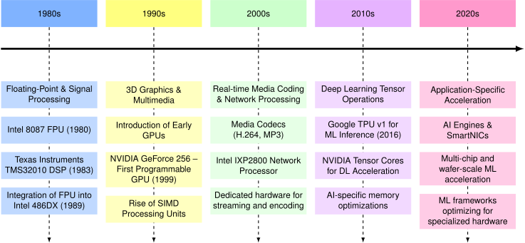](https://mlsysbook.ai/contents/core/hw_acceleration/284c5b21bbcb3bac7a47ffbf3fc71aecca5b7daa.svg "Figure 1: Hardware Specialization Trajectory: Computing architectures progressively incorporate specialized accelerators to address emerging performance bottlenecks and workload demands, mirroring a historical pattern from floating-point units to graphics processors and, ultimately, machine learning accelerators. This evolution reflects a strategy for improving computational efficiency by tailoring hardware to specific task characteristics and advancing increasingly complex applications.")
Figure 1: **Hardware Specialization Trajectory**: Computing architectures progressively incorporate specialized accelerators to address emerging performance bottlenecks and workload demands, mirroring a historical pattern from floating-point units to graphics processors and, ultimately, machine learning accelerators. This evolution reflects a strategy for improving computational efficiency by tailoring hardware to specific task characteristics and advancing increasingly complex applications.
### Parallel Computing and Graphics Processing
The principles established through floating-point acceleration provided a blueprint for addressing emerging computational challenges. As computing applications diversified, new computational patterns emerged that exceeded the capabilities of general-purpose processors. This expansion of specialized computing manifested across multiple domains, each contributing unique insights to hardware acceleration strategies.
Graphics processing emerged as a primary driver of hardware specialization in the 1990s. Early graphics accelerators focused on specific operations like bitmap transfers and polygon filling. The introduction of programmable graphics pipelines with NVIDIA’s GeForce 256 in 1999 represented a significant advancement in specialized computing. Graphics Processing Units (GPUs) demonstrated how parallel processing architectures could efficiently handle data-parallel workloads, achieving 50-100\\(\\times\\) speedups in 3D rendering tasks like texture mapping and vertex transformation. By 2004, high-end GPUs could process over 100 million polygons per second ([Owens et al. 2008](https://mlsysbook.ai/contents/core/hw_acceleration/hw_acceleration.html#ref-owens2008gpu)
).
Lyons, Richard G. 2011. _Understanding Digital Signal Processing_. 3rd ed. Prentice Hall.
Concurrently, Digital Signal Processing (DSP) processors established parallel data path architectures with specialized multiply-accumulate units and circular buffers optimized for filtering and transform operations. Texas Instruments’ TMS32010 (1983) demonstrated how domain-specific instruction sets could dramatically improve performance for signal processing applications ([Lyons 2011](https://mlsysbook.ai/contents/core/hw_acceleration/hw_acceleration.html#ref-lyons2011understanding)
).
Network processing introduced additional patterns of specialization. Network processors developed unique architectures to handle packet processing at line rate, incorporating multiple processing cores, specialized packet manipulation units, and sophisticated memory management systems. Intel’s IXP2800 network processor demonstrated how multiple levels of hardware specialization could be combined to address complex processing requirements.
These diverse domains of specialization exhibit several common characteristics:
1. Identification of domain-specific computational patterns
2. Development of specialized processing elements and memory hierarchies
3. Creation of domain-specific programming models
4. Progressive evolution toward more flexible architectures
This period of expanding specialization demonstrated that hardware acceleration strategies could address diverse computational requirements across multiple domains. The GPU’s success in parallelizing 3D graphics pipelines enabled its subsequent adoption for training deep neural networks, exemplified by AlexNet[5](https://mlsysbook.ai/contents/core/hw_acceleration/hw_acceleration.html#fn5)
in 2012, which executed on consumer-grade NVIDIA GPUs. DSP innovations in low-power signal processing facilitated real-time inference on edge devices, including voice assistants and wearables. These domains informed ML hardware designs and established that accelerators could be deployed across both cloud and embedded contexts, principles that continue to influence contemporary AI ecosystem development.
5 **AlexNet’s GPU Revolution**: AlexNet’s breakthrough wasn’t just algorithmic. It proved GPUs could train deep networks 10\\(\\times\\) faster than CPUs ([Krizhevsky, Sutskever, and Hinton 2017](https://mlsysbook.ai/contents/core/hw_acceleration/hw_acceleration.html#ref-krizhevsky2012alexnet)
). The team split the 8-layer network across two NVIDIA GTX 580s (512 cores each), reducing training time from weeks to days. This success triggered the “deep learning gold rush” and established NVIDIA as the default AI hardware company, with GPU sales for data centers growing from $200 million to $47 billion by 2024. Modern GPUs like the NVIDIA H100 contains 16,896 streaming processors, demonstrating the massive scaling in parallel processing capability since AlexNet’s era.
Krizhevsky, Alex, Ilya Sutskever, and Geoffrey E. Hinton. 2017. “ImageNet Classification with Deep Convolutional Neural Networks.” _Communications of the ACM_ 60 (6): 84–90. [https://doi.org/10.1145/3065386](https://doi.org/10.1145/3065386)
.
### Emergence of Domain-Specific Architectures
The emergence of domain-specific architectures (DSA)[6](https://mlsysbook.ai/contents/core/hw_acceleration/hw_acceleration.html#fn6)
marks a shift in computer system design, driven by two factors: the breakdown of traditional scaling laws and the increasing computational demands of specialized workloads. The slowdown of Moore’s Law[7](https://mlsysbook.ai/contents/core/hw_acceleration/hw_acceleration.html#fn7)
, which previously ensured predictable enhancements in transistor density every 18 to 24 months, and the end of Dennard scaling[8](https://mlsysbook.ai/contents/core/hw_acceleration/hw_acceleration.html#fn8)
, which permitted frequency increases without corresponding power increases, created a performance and efficiency bottleneck in general-purpose computing. As John Hennessy and David Patterson noted in their 2017 Turing Lecture ([Hennessy and Patterson 2019](https://mlsysbook.ai/contents/core/hw_acceleration/hw_acceleration.html#ref-HennessyPatterson2017Turing)
), these limitations signaled the onset of a new era in computer architecture, one centered on domain-specific solutions that optimize hardware for specialized workloads.
6 **Domain-Specific Architectures (DSA)**: Computing architectures optimized for specific application domains rather than general-purpose computation. Unlike CPUs designed for flexibility, DSAs sacrifice programmability for dramatic efficiency gains. Google’s TPU achieves 15-30\\(\\times\\) better performance per watt than GPUs for neural networks, while video codecs provide 100-1000\\(\\times\\) improvements over software decoding. The 2018 Turing Award recognized this shift as the defining trend in modern computer architecture.
7 **Moore’s Law**: Intel co-founder Gordon Moore’s 1965 observation that transistor density doubles every 18-24 months. This exponential scaling drove computing progress for 50 years, enabling everything from smartphones to supercomputers. However, physical limits around 2005 slowed this pace dramatically. Modern 3 nm chips cost $20 billion to develop versus $3 million in 1999, forcing the industry toward specialized architectures.
8 **Dennard Scaling**: Robert Dennard’s 1974 principle that as transistors shrink, their power density remains constant, allowing higher frequencies without increased power consumption. This enabled CPUs to reach 3+ GHz by 2005. However, quantum effects and leakage current ended Dennard scaling around 2005, forcing architects to prioritize efficiency over raw speed and leading to the multi-core revolution.
Hennessy, John L., and David A. Patterson. 2019. “A New Golden Age for Computer Architecture.” _Communications of the ACM_ 62 (2): 48–60. [https://doi.org/10.1145/3282307](https://doi.org/10.1145/3282307)
.
Historically, improvements in processor performance depended on semiconductor process scaling and increasing clock speeds. However, as power density limitations restricted further frequency scaling, and as transistor miniaturization encountered increasing physical and economic constraints, architects explored alternative approaches to sustain computational growth. This resulted in a shift toward domain-specific architectures, which dedicate silicon resources to optimize computation for specific application domains, trading flexibility for efficiency.
Domain-specific architectures achieve superior performance and energy efficiency through several key principles:
1. **Customized data paths**: Design processing paths specifically optimized for target application patterns, enabling direct hardware execution of common operations. For example, matrix multiplication units in AI accelerators implement systolic arrays—grid-like networks of processing elements that rhythmically compute and pass data through neighboring units—tailored for neural network computations.
2. **Specialized memory hierarchies**: Optimize memory systems around domain-specific access patterns and data reuse characteristics. This includes custom cache configurations, prefetching logic, and memory controllers tuned for expected workloads.
3. **Reduced instruction overhead**: Implement domain-specific instruction sets that minimize decode and dispatch complexity by encoding common operation sequences into single instructions. This improves both performance and energy efficiency.
4. **Direct hardware implementation**: Create dedicated circuit blocks that natively execute frequently used operations without software intervention. This eliminates instruction processing overhead and maximizes throughput.
These principles achieve compelling demonstration in modern smartphones. Modern smartphones can decode 4K video at 60 frames per second while consuming only a few watts of power, despite video processing requiring billions of operations per second. This efficiency is achieved through dedicated hardware video codecs that implement industry standards such as H.264/AVC (introduced in 2003) and H.265/HEVC (finalized in 2013) ([Sullivan et al. 2012](https://mlsysbook.ai/contents/core/hw_acceleration/hw_acceleration.html#ref-sullivan2012overview)
). These specialized circuits provide 100–1000\\(\\times\\) improvements in both performance and power efficiency compared to software-based decoding on general-purpose processors.
Sullivan, Gary J., Jens-Rainer Ohm, Woo-Jin Han, and Thomas Wiegand. 2012. “Overview of the High Efficiency Video Coding (HEVC) Standard.” _IEEE Transactions on Circuits and Systems for Video Technology_ 22 (12): 1649–68. [https://doi.org/10.1109/tcsvt.2012.2221191](https://doi.org/10.1109/tcsvt.2012.2221191)
.
Shang, J., G. Wang, and Y. Liu. 2018. “Accelerating Genomic Data Analysis with Domain-Specific Architectures.” _IEEE Transactions on Computers_ 67 (7): 965–78. [https://doi.org/10.1109/TC.2018.2799212](https://doi.org/10.1109/TC.2018.2799212)
.
9 **Application-Specific Integrated Circuits (ASICs)**: Custom silicon chips designed for a single application, offering maximum efficiency by eliminating unused features. Bitcoin mining ASICs achieve 100,000\\(\\times\\) better energy efficiency than CPUs for SHA-256 hashing. However, their inflexibility means they become worthless if algorithms change. An estimated $5 billion in Ethereum mining ASICs became obsolete when Ethereum switched to proof-of-stake in September 2022.
Bedford Taylor, Michael. 2017. “The Evolution of Bitcoin Hardware.” _Computer_ 50 (9): 58–66. [https://doi.org/10.1109/mc.2017.3571056](https://doi.org/10.1109/mc.2017.3571056)
.
The trend toward specialization continues to accelerate, with new architectures emerging for an expanding range of domains. Genomics processing benefits from custom accelerators that optimize sequence alignment and variant calling, reducing the time required for DNA analysis ([Shang, Wang, and Liu 2018](https://mlsysbook.ai/contents/core/hw_acceleration/hw_acceleration.html#ref-Shang2018GenomicsAccel)
). Similarly, blockchain computation has produced application-specific integrated circuits (ASICs)[9](https://mlsysbook.ai/contents/core/hw_acceleration/hw_acceleration.html#fn9)
optimized for cryptographic hashing, substantially increasing the efficiency of mining operations ([Bedford Taylor 2017](https://mlsysbook.ai/contents/core/hw_acceleration/hw_acceleration.html#ref-Taylor2017ASICMining)
). These examples demonstrate that domain-specific architecture represents a fundamental transformation in computing systems, offering tailored solutions that address the growing complexity and diversity of modern computational workloads.
### Machine Learning Hardware Specialization
Machine learning constitutes a computational domain with unique characteristics that have driven the development of specialized hardware architectures. Unlike traditional computing workloads that exhibit irregular memory access patterns and diverse instruction streams, neural networks are characterized by predictable patterns: dense matrix multiplications, regular data flow, and tolerance for reduced precision. These characteristics enable specialized hardware optimizations that would be ineffective for general-purpose computing but provide substantial speedups for ML workloads.
**Definition:** ML Accelerator
**_Machine Learning Accelerators_** are specialized computing hardware optimized for the _computational patterns_ of neural networks, achieving superior _performance per watt_ through _parallel processing_, _specialized memory hierarchies_, and _reduced-precision arithmetic_.
Machine learning computational requirements reveal limitations in traditional processors. CPUs achieve only 5-10% utilization on neural network workloads, delivering approximately 100 GFLOPS[10](https://mlsysbook.ai/contents/core/hw_acceleration/hw_acceleration.html#fn10)
while consuming hundreds of watts. This inefficiency results from architectural mismatches: CPUs optimize for single-thread performance and irregular memory access, while neural networks require massive parallelism and predictable data streams. The memory bandwidth[11](https://mlsysbook.ai/contents/core/hw_acceleration/hw_acceleration.html#fn11)
constraint becomes particularly severe: a single neural network layer may require accessing gigabytes of parameters, overwhelming CPU cache hierarchies[12](https://mlsysbook.ai/contents/core/hw_acceleration/hw_acceleration.html#fn12)
designed for kilobyte-scale working sets.
10 **GFLOPS (Giga Floating-Point Operations Per Second)**: A measure of computational throughput representing one billion floating-point operations per second. TOPS (Tera Operations Per Second) represents one trillion operations per second, typically used for integer operations in AI accelerators.
11 **Memory Bandwidth**: The rate at which data can be transferred between memory and processors, measured in GB/s or TB/s. AI workloads are often bandwidth-bound rather than compute-bound. NVIDIA H100 provides 3.35 TB/s (approximately 40\\(\\times\\) faster than typical DDR5-4800 configurations at ~80 GB/s) because neural networks require constant weight access, making memory bandwidth the primary bottleneck in many AI applications.
12 **Cache Hierarchy**: Multi-level memory system with L1, L2, and L3 caches providing progressively larger capacity but higher latency. CPUs optimize for 32-64KB L1 caches with <1ns access time, but neural networks need gigabytes of weights that cannot fit in cache, causing frequent expensive DRAM accesses (100ns latency) and degrading performance from 90%+ cache hit rates to <10%.
The energy economics of data movement influence accelerator design. Accessing data from DRAM requires approximately 640 picojoules while performing a multiply-accumulate operation consumes only 3.7 pJ, approximately a 173× penalty (specific values vary by technology node and design) that establishes minimizing data movement as the primary optimization target. This disparity explains the progression from repurposed graphics processors to purpose-built neural network accelerators. GPUs achieve 15,000+ GFLOPS through massive parallelism but encounter efficiency challenges from their graphics heritage. TPUs and other custom accelerators achieve utilization above 85% by implementing systolic arrays and other architectures that maximize data reuse while minimizing movement.
Training and inference present distinct computational profiles that influence accelerator design. Training requires high-precision arithmetic (FP32 or FP16) for gradient computation and weight updates, bidirectional data flow for backpropagation[13](https://mlsysbook.ai/contents/core/hw_acceleration/hw_acceleration.html#fn13)
, and large memory capacity for storing activations. Inference can exploit reduced precision (INT8 or INT4), requires only forward computation, and prioritizes latency over throughput[14](https://mlsysbook.ai/contents/core/hw_acceleration/hw_acceleration.html#fn14)
. These differences drive specialized architectures: training accelerators maximize FLOPS and memory bandwidth, while inference accelerators optimize for energy efficiency and deterministic latency.
13 **Backpropagation**: The key training algorithm that computes gradients by propagating errors backwards through the network using the chain rule. Unlike forward inference which only needs current layer outputs, backpropagation requires storing all intermediate activations from forward pass, increasing memory requirements 2-3\\(\\times\\) and necessitating bidirectional data flow that complicates accelerator design.
14 **Latency vs Throughput**: Latency measures response time for a single request (milliseconds), while throughput measures requests processed per unit time (requests/second). Training optimizes throughput to process large batches efficiently, while inference prioritizes latency for real-time responses. A GPU might achieve 1000 images/second (high throughput) but take 50ms per image (high latency), making it unsuitable for real-time applications requiring <10ms response times.
Deployment context shapes architectural choices. Datacenter accelerators accept 700-watt power budgets to maximize throughput for training massive models. Edge devices must deliver real-time inference within milliwatt constraints, driving architectures that eliminate every unnecessary data movement. Mobile processors balance performance with battery life, while automotive systems prioritize deterministic response times for safety-critical applications. This diversity has produced a rich ecosystem of specialized accelerators, each optimized for specific deployment scenarios and computational requirements.
In data centers, training accelerators such as NVIDIA H100 and Google TPUv4 reduce model development from weeks to days through massive parallelism and high-bandwidth memory systems. These systems prioritize raw computational throughput, accepting 700-watt power consumption to achieve petaflop-scale performance. The economics support this trade-off—reducing training time from months to days can reduce millions in operational costs and accelerate time-to-market for AI applications.
At the opposite extreme, edge deployment requires different optimization strategies. Processing-in-memory architectures eliminate data movement by integrating compute directly with memory. Dynamic voltage scaling reduces power by 50-90% during low-intensity operations. Neuromorphic designs process only changing inputs, achieving 1000× power reduction for temporal workloads. These techniques enable sophisticated AI models to operate continuously on battery power, supporting applications from smartphone photography to autonomous sensors that function for years without external power.
The success of application-specific accelerators demonstrates that no single architecture can efficiently address all ML workloads. The 156 billion edge devices projected by 2030 will require architectures optimized for energy efficiency and real-time guarantees, while cloud-scale training will continue advancing the boundaries of computational throughput. This diversity drives continued innovation in specialized architectures, each optimized for its specific deployment context and computational requirements.
The evolution of specialized hardware architectures illustrates a principle in computing systems: as computational patterns emerge and mature, hardware specialization follows to achieve optimal performance and energy efficiency. This progression appears clearly in machine learning acceleration, where domain-specific architectures have evolved to meet the increasing computational demands of machine learning models. Unlike general-purpose processors, which prioritize flexibility, specialized accelerators optimize execution for well-defined workloads, balancing performance, energy efficiency, and integration with software frameworks.
[Table 1](https://mlsysbook.ai/contents/core/hw_acceleration/hw_acceleration.html#tbl-hw-evolution)
summarizes key milestones in the evolution of hardware specialization, showing how each era produced architectures tailored to the prevailing computational demands. While these accelerators initially emerged to optimize domain-specific workloads, including floating-point operations, graphics rendering, and media processing, they also introduced architectural strategies that persist in contemporary systems. The specialization principles outlined in earlier generations now underpin the design of modern AI accelerators. Understanding this historical trajectory provides context for analyzing how hardware specialization continues to enable scalable, efficient execution of machine learning workloads across diverse deployment environments.
Table 1: **Hardware Specialization Trends**: Successive computing eras progressively integrate specialized hardware to accelerate prevalent workloads, moving from general-purpose CPUs to domain-specific architectures and ultimately to customizable AI accelerators. This evolution reflects a fundamental principle: tailoring hardware to computational patterns improves performance and energy efficiency, driving innovation in machine learning systems.
| | | | |
| --- | --- | --- | --- |
| **1980s** | Floating-Point & Signal Processing | FPU, DSP | * Single-purpose engines
* Focused instruction sets
* Coprocessor interfaces |
| **1990s** | 3D Graphics & Multimedia | GPU, SIMD Units | * Many identical compute units
* Regular data patterns
* Wide memory interfaces |
| **2000s** | Real-time Media Coding | Media Codecs, Network Processors | * Fixed-function pipelines
* High throughput processing
* Power-performance optimization |
| **2010s** | Deep Learning Tensor Operations | TPU, GPU Tensor Cores | * Matrix multiplication units
* Massive parallelism
* Memory bandwidth optimization |
| **2020s** | Application-Specific Acceleration | ML Engines, Smart NICs, Domain Accelerators | * Workload-specific datapaths
* Customized memory hierarchies
* Application-optimized designs |
This historical progression reveals a recurring pattern: each wave of hardware specialization responded to a computational bottleneck, whether graphics rendering, media encoding, or neural network inference. What distinguishes the 2020s is not just specialization, but its pervasiveness: AI accelerators now underpin everything from product recommendations on YouTube to object detection in autonomous vehicles. Unlike earlier accelerators, today’s AI hardware must integrate tightly with dynamic software frameworks and scale across cloud-to-edge deployments. The table illustrates not just the past but also the trajectory toward increasingly tailored, high-impact computing platforms.
For AI acceleration, this transition has introduced challenges that extend well beyond hardware design. Machine learning accelerators must integrate seamlessly into ML workflows by aligning with optimizations at multiple levels of the computing stack. They must operate effectively with widely adopted frameworks such as TensorFlow, PyTorch, and JAX, ensuring that deployment is smooth and consistent across varied hardware platforms. Compiler and runtime support become necessary; advanced optimization techniques, such as graph-level transformations, kernel fusion, and memory scheduling, are critical for using the full potential of these specialized accelerators.
Scalability drives additional complexity as AI accelerators deploy across diverse environments from high-throughput data centers to resource-constrained edge and mobile devices, requiring tailored performance tuning and energy efficiency strategies. Integration into heterogeneous computing[15](https://mlsysbook.ai/contents/core/hw_acceleration/hw_acceleration.html#fn15)
environments demands interoperability that enables specialized units to coordinate effectively with conventional CPUs and GPUs in distributed systems.
15 **Heterogeneous Computing**: Computing systems that combine different types of processors (CPUs, GPUs, TPUs, FPGAs) to optimize performance for diverse workloads. Modern data centers mix x86 CPUs for control tasks, GPUs for training, and TPUs for inference. Programming heterogeneous systems requires frameworks like OpenCL or CUDA that can coordinate execution across different architectures, but offers 10-100\\(\\times\\) efficiency gains by matching each task to optimal hardware.
AI accelerators represent a system-level transformation that requires tight hardware-software coupling. This transformation manifests in three specific computational patterns, compute primitives, that drive accelerator design decisions. Understanding these primitives determines the architectural features that enable 100-1000\\(\\times\\) performance improvements through coordinated hardware specialization and software optimization strategies examined in subsequent sections.
The evolution from floating-point coprocessors to AI accelerators reveals a consistent pattern: computational bottlenecks drive specialized hardware development. Where the Intel 8087 addressed floating-point operations that consumed 80% of scientific computing time, modern AI workloads present an even more extreme case. Matrix multiplications and convolutions constitute over 95% of neural network computation. This concentration of computational demand creates unprecedented opportunities for specialization, explaining why AI accelerators achieve 100-1000\\(\\times\\) performance improvements over general-purpose processors.
The specialization principles established through decades of hardware evolution identifying dominant operations, creating dedicated datapaths, and optimizing memory access patterns now guide AI accelerator design. However, neural networks introduce unique characteristics that demand new architectural approaches: massive parallelism in matrix operations, predictable data access patterns enabling prefetching, and tolerance for reduced precision that allows aggressive optimization. Understanding these computational patterns, which we term AI compute primitives, helps comprehend how modern accelerators transform the theoretical efficiency gains from **[Chapter 10: Model Optimizations](https://mlsysbook.ai/contents/core/optimizations/optimizations.html#sec-model-optimizations)
** into practical performance improvements. These hardware-software optimizations become critical in deployment scenarios ranging from **[Chapter 2: ML Systems](https://mlsysbook.ai/contents/core/ml_systems/ml_systems.html#sec-ml-systems)
** edge devices to cloud-scale inference systems.
Before examining these computational primitives in detail, we need to understand the architectural organization that enables their efficient execution. Modern AI accelerators achieve their dramatic performance improvements through a carefully orchestrated hierarchy of specialized components operating in concert. The architecture comprises three subsystems, each addressing distinct aspects of the computational challenge.
The processing substrate consists of an array of processing elements, each containing dedicated computational units optimized for specific operations: tensor cores execute matrix multiplication, vector units perform element-wise operations, and special function units compute activation functions. These processing elements are organized in a grid topology that enables massive parallelism, with dozens to hundreds of units operating simultaneously on different portions of the computation, exploiting the data-level parallelism inherent in neural network workloads.
The memory hierarchy forms an equally critical architectural component. High-bandwidth memory provides the aggregate throughput required to sustain these numerous processing elements, while a multi-level cache hierarchy from shared L2 caches down to per-element L1 caches and scratchpads minimizes the energy cost of data movement. This hierarchical organization embodies a design principle: in AI accelerators, data movement typically consumes more energy than computation itself, necessitating architectural strategies that prioritize data reuse by maintaining frequently accessed values, including weights and partial results, in proximity to compute units.
The host interface establishes connectivity between the specialized accelerator and the broader computing system, enabling coordination between general-purpose CPUs that manage program control flow and the accelerator that executes computationally intensive neural network operations. This architectural partitioning reflects specialization at the system level: CPUs address control flow, conditional logic, and system coordination, while accelerators focus on the regular, massively parallel arithmetic operations that dominate neural network execution.
[Figure 2](https://mlsysbook.ai/contents/core/hw_acceleration/hw_acceleration.html#fig-accelerator-anatomy)
illustrates this architectural organization, showing how specialized compute units, hierarchical memory subsystems, and host connectivity integrate to form a system optimized for AI workloads.
[](https://mlsysbook.ai/contents/core/hw_acceleration/1559765a6107b67182c20d4134c01f5bf2e29375.svg "Figure 2: Anatomy of a Modern AI Accelerator: AI accelerators integrate specialized processing elements containing tensor cores, vector units, and special function units, supported by a hierarchical memory system from high-bandwidth memory down to local caches. This architecture maximizes data reuse and parallel execution while minimizing energy-intensive data movement, forming the foundation for 100-1000× performance improvements over general-purpose processors.")
Figure 2: **Anatomy of a Modern AI Accelerator**: AI accelerators integrate specialized processing elements containing tensor cores, vector units, and special function units, supported by a hierarchical memory system from high-bandwidth memory down to local caches. This architecture maximizes data reuse and parallel execution while minimizing energy-intensive data movement, forming the foundation for 100-1000× performance improvements over general-purpose processors.
**Self-Check: Question 1.2**
1. Which of the following best describes the primary motivation for the development of specialized hardware accelerators in computing?
1. To reduce the cost of general-purpose processors
2. To increase the flexibility of computing systems
3. To handle increasingly complex computational workloads efficiently
4. To simplify the programming models for developers
2. Explain how the evolution of specialized hardware has influenced the design of modern machine learning accelerators.
3. True or False: The integration of specialized functions into general-purpose processors is a common trend observed in the evolution of computing architectures.
4. What is a key trade-off introduced by the use of specialized hardware accelerators?
1. Increased flexibility in programming
2. Reduced programming complexity
3. Higher energy consumption
4. Reduced silicon area utilization
5. In a production system, how might the choice of hardware accelerators impact the deployment of machine learning models?
[See Answers →](https://mlsysbook.ai/contents/core/hw_acceleration/hw_acceleration.html#quiz-answer-sec-ai-acceleration-evolution-hardware-specialization-1d21)
AI Compute Primitives
---------------------
Understanding how hardware evolved toward AI-specific designs requires examining the computational patterns that drove this specialization. The transition from general-purpose CPUs achieving 100 GFLOPS to specialized accelerators delivering 100,000+ GFLOPS reflects architectural optimization for specific computational patterns that dominate machine learning workloads. These patterns, which we term compute primitives, appear repeatedly across all neural network architectures regardless of application domain or model size.
Modern neural networks are built upon a small number of core computational patterns. Regardless of the layer type—whether fully connected, convolutional, or attention-based layers—the underlying operation typically involves multiplying input values by learned weights and accumulating the results. This repeated multiply-accumulate process dominates neural network execution and defines the arithmetic foundation of AI workloads. The regularity and frequency of these operations have led to the development of AI compute primitives: hardware-level abstractions optimized to execute these core computations with high efficiency.
Neural networks exhibit highly structured, data-parallel computations that enable architectural specialization. Building on the parallelization principles established in [Section 1.2.2](https://mlsysbook.ai/contents/core/hw_acceleration/hw_acceleration.html#sec-ai-acceleration-parallel-computing-graphics-processing-66b1)
, these patterns emphasize predictable data reuse and fixed operation sequences. AI compute primitives distill these patterns into reusable architectural units that support high-throughput and energy-efficient execution.
This decomposition is illustrated in [Listing 1](https://mlsysbook.ai/contents/core/hw_acceleration/hw_acceleration.html#lst-dense_layer_def)
, which defines a dense layer at the framework level.
Listing 1: **Dense Layer Definition**: Defines a dense layer using a high-level API, illustrating how neural networks implement parallel transformations across input tensors.
dense = Dense(512)(input_tensor)
This high-level call expands into mathematical operations is shown in [Listing 2](https://mlsysbook.ai/contents/core/hw_acceleration/hw_acceleration.html#lst-dense_expansion)
.
Listing 2: **Layer Computation**: Neural networks compute each layer’s output via weighted input summation followed by an activation function transformation.
output = matmul(input_weights) + bias
output = activation(output)
At the processor level, the computation reduces to nested loops that multiply inputs and weights, sum the results, and apply a nonlinear function, as shown in [Listing 3](https://mlsysbook.ai/contents/core/hw_acceleration/hw_acceleration.html#lst-loop_level_dense)
.
Listing 3: **Nested Loops**: Computes output values through sequential matrix multiplications and bias additions, followed by activation function application to produce final outputs.
for n in range(batch_size):
for m in range(output_size):
sum = bias[m]
for k in range(input_size):
sum += input[n, k] * weights[k, m]
output[n, m] = activation(sum)
This transformation reveals four computational characteristics: data-level parallelism enabling simultaneous execution, structured matrix operations defining computational workloads, predictable data movement patterns driving memory optimization, and frequent nonlinear transformations motivating specialized function units.
The design of AI compute primitives follows three architectural criteria. First, the primitive must be used frequently enough to justify dedicated hardware resources. Second, its specialized implementation must offer substantial performance or energy efficiency gains relative to general-purpose alternatives. Third, the primitive must remain stable across generations of neural network architectures to ensure long-term applicability. These considerations shape the inclusion of primitives such as vector operations, matrix operations, and special function units in modern ML accelerators. Together, they serve as the architectural foundation for efficient and scalable neural network execution.
### Vector Operations
Vector operations provide the first level of hardware acceleration by processing multiple data elements simultaneously. This parallelism exists at multiple scales, from individual neurons to entire layers, making vector processing essential for efficient neural network execution. Framework-level code translates to hardware instructions, revealing the critical role of vector processing in neural accelerators.
#### High-Level Framework Operations
Machine learning frameworks hide hardware complexity through high-level abstractions. These abstractions decompose into progressively lower-level operations, revealing opportunities for hardware acceleration. One such abstraction is shown in [Listing 4](https://mlsysbook.ai/contents/core/hw_acceleration/hw_acceleration.html#lst-linear_layer_highlevel)
, which illustrates the execution flow of a linear layer.
Listing 4: **Linear Layer**: Neural networks transform input data into a higher-dimensional space using linear mappings to enable complex feature extraction.
layer = nn.Linear(256, 512) # 256 inputs to
# 512 outputs
output = layer(input_tensor) # Process a batch of inputs
This abstraction represents a fully connected layer that transforms input features through learned weights. To understand how hardware acceleration opportunities emerge, [Listing 5](https://mlsysbook.ai/contents/core/hw_acceleration/hw_acceleration.html#lst-linear_math_internal)
shows how the framework translates this high-level expression into mathematical operations.
Listing 5: **Fully Connected Layer**: Each output is computed as a weighted sum of all inputs plus a bias, followed by an activation function transformation. Linear transformations enable complex model architectures in neural networks.
Z = matmul(weights, input) + bias # Each output needs all inputs
output = activation(Z) # Transform each result
These mathematical operations further decompose into explicit computational steps during processor execution. [Listing 6](https://mlsysbook.ai/contents/core/hw_acceleration/hw_acceleration.html#lst-loop_linear_layer)
illustrates the nested loops that implement these multiply-accumulate operations.
Listing 6: **Linear Layer Computation**: Each output neuron is computed by summing weighted inputs from all features, followed by an activation function application. Understanding this process helps in grasping the fundamental building blocks of neural networks.
for batch in range(32): # Process 32 samples at once
for out_neuron in range(512): # Compute each output neuron
sum = 0.0
for in_feature in range(256): # Each output needs
# all inputs
sum += input[batch, in_feature] *
weights[out_neuron, in_feature]
output[batch, out_neuron] = activation(sum +
bias[out_neuron])
#### Sequential Scalar Execution
Traditional scalar processors execute these operations sequentially, processing individual values one at a time. For the linear layer example above with a batch of 32 samples, computing the outputs requires over 4 million multiply-accumulate operations. Each operation involves loading an input value and a weight value, multiplying them, and accumulating the result. This sequential approach becomes highly inefficient when processing the massive number of identical operations required by neural networks.
Recognizing this inefficiency, modern processors leverage vector processing to transform execution patterns fundamentally.
#### Parallel Vector Execution
Vector processing units achieve this transformation by operating on multiple data elements simultaneously. [Listing 7](https://mlsysbook.ai/contents/core/hw_acceleration/hw_acceleration.html#lst-riscv_vector_mac)
demonstrates this approach using RISC-V[16](https://mlsysbook.ai/contents/core/hw_acceleration/hw_acceleration.html#fn16)
assembly code that showcases modern vector processing capabilities.
16 **RISC-V for AI**: RISC-V, the open-source instruction set architecture from UC Berkeley (2010), is becoming important for AI accelerators because it’s freely customizable. Companies like SiFive and Google have created RISC-V chips with custom AI extensions. Unlike proprietary architectures, RISC-V allows hardware designers to add specialized ML instructions without licensing fees, potentially democratizing AI hardware development beyond the current duopoly of x86 and ARM.
Listing 7: **Vectorized Multiply-Accumulate Loop**: This loop showcases how RISC-V vector instructions enable efficient batch processing by performing 8 multiply-add operations simultaneously, reducing computational latency in neural network training. _Source: RISC-V Architecture Manual_
vsetvli t0, a0, e32 # Process 8 elements at once
loop_batch:
loop_neuron:
vxor.vv v0, v0, v0 # Clear 8 accumulators
loop_feature:
vle32.v v1, (in_ptr) # Load 8 inputs together
vle32.v v2, (wt_ptr) # Load 8 weights together
vfmacc.vv v0, v1, v2 # 8 multiply-adds at once
add in_ptr, in_ptr, 32 # Move to next 8 inputs
add wt_ptr, wt_ptr, 32 # Move to next 8 weights
bnez feature_cnt, loop_feature
This vector implementation processes eight data elements in parallel, reducing both computation time and energy consumption. Vector load instructions transfer eight values simultaneously, maximizing memory bandwidth utilization. The vector multiply-accumulate instruction processes eight pairs of values in parallel, dramatically reducing the total instruction count from over 4 million to approximately 500,000.
To clarify how vector instructions map to common deep learning patterns, [Table 2](https://mlsysbook.ai/contents/core/hw_acceleration/hw_acceleration.html#tbl-vector)
introduces key vector operations and their typical applications in neural network computation. These operations, such as reduction, gather, scatter, and masked operations, are frequently encountered in layers like pooling, embedding lookups, and attention mechanisms. This terminology is necessary for interpreting how low-level vector hardware accelerates high-level machine learning workloads.
Table 2: **Vector Operations**: Neural network layers frequently utilize core vector operations such as reduction, gather, and scatter to accelerate computation and efficiently process data in parallel; these operations clarify how low-level hardware optimizations map to high-level machine learning algorithms. These operations enable efficient implementation of common layers like pooling, embedding lookups, and attention mechanisms within deep learning models.
| | | |
| --- | --- | --- |
| **Reduction** | Combines elements across a vector (e.g., sum, max) | Pooling layers, attention score computation |
| **Gather** | Loads multiple non-consecutive memory elements | Embedding lookups, sparse operations |
| **Scatter** | Writes to multiple non-consecutive memory locations | Gradient updates for embeddings |
| **Masked operations** | Selectively operates on vector elements | Attention masks, padding handling |
| **Vector-scalar broadcast** | Applies scalar to all vector elements | Bias addition, scaling operations |
Vector processing efficiency gains extend beyond instruction count reduction. Memory bandwidth utilization improves as vector loads transfer multiple values per operation. Energy efficiency increases because control logic is shared across multiple operations. These improvements compound across the deep layers of modern neural networks, where billions of operations execute for each forward pass.
#### Vector Processing History
The principles underlying vector operations have long been central to high-performance computing. In the 1970s and 1980s, vector processors emerged as an architectural solution for scientific computing, weather modeling, and physics simulations, where large arrays of data required efficient parallel processing. Early systems such as the Cray-1[17](https://mlsysbook.ai/contents/core/hw_acceleration/hw_acceleration.html#fn17)
, one of the first commercially successful supercomputers, introduced dedicated vector units to perform arithmetic operations on entire data vectors in a single instruction. These vector units dramatically improved computational throughput compared to traditional scalar execution ([Jordan 1982](https://mlsysbook.ai/contents/core/hw_acceleration/hw_acceleration.html#ref-jordan1982guide)
).
17 **Cray-1 Vector Legacy**: The Cray-1 (1975) cost $8.8 million (approximately $40-45 million in 2024 dollars) but could perform 160 million floating-point operations per second—1000x faster than typical computers. Its 64-element vector registers and pipelined vector units established the architectural template that modern AI accelerators still follow: process many data elements simultaneously with specialized hardware pipelines.
Jordan, T. L. 1982. “A Guide to Parallel Computation and Some Cray-1 Experiences.” In _Parallel Computations_, 1–50. Elsevier. [https://doi.org/10.1016/b978-0-12-592101-5.50006-3](https://doi.org/10.1016/b978-0-12-592101-5.50006-3)
.
These concepts have reemerged in machine learning, where neural networks exhibit structure well suited to vectorized execution. The same operations, such as vector addition, multiplication, and reduction, that once accelerated numerical simulations now drive the execution of machine learning workloads. While the scale and specialization of modern AI accelerators differ from their historical predecessors, the underlying architectural principles remain the same. The resurgence of vector processing in neural network acceleration highlights its utility for achieving high computational efficiency.
Vector operations establish the foundation for neural network acceleration by enabling efficient parallel processing of independent data elements. While vector operations excel at element-wise transformations like activation functions, neural networks also require structured computations that combine multiple input features to produce output features, transformations that naturally express themselves as matrix operations. This need for coordinated computation across multiple dimensions simultaneously leads to the next architectural primitive: matrix operations.
### Matrix Operations
Matrix operations form the computational workhorse of neural networks, transforming high-dimensional data through structured patterns of weights, activations, and gradients ([Goodfellow, Courville, and Bengio 2013](https://mlsysbook.ai/contents/core/hw_acceleration/hw_acceleration.html#ref-Goodfellow-et-al-2016)
). While vector operations process elements independently, matrix operations orchestrate computations across multiple dimensions simultaneously. These operations reveal patterns that drive hardware acceleration strategies.
#### Matrix Operations in Neural Networks
Neural network computations decompose into hierarchical matrix operations. As shown in [Listing 8](https://mlsysbook.ai/contents/core/hw_acceleration/hw_acceleration.html#lst-linear_matrix_hierarchy)
, a linear layer demonstrates this hierarchy by transforming input features into output neurons over a batch.
Listing 8: **Matrix Operations**: Neural networks perform transformations using matrix multiplications and biases to achieve output predictions. Training requires careful management of input batches and activation functions to optimize model performance.
layer = nn.Linear(256, 512) # Layer transforms 256 inputs to
# 512 outputs
output = layer(input_batch) # Process a batch of 32 samples
# Framework Internal: Core operations
Z = matmul(weights, input) # Matrix: transforms [256 x 32]
# input to [512 x 32] output
Z = Z + bias # Vector: adds bias to each
# output independently
output = relu(Z) # Vector: applies activation to
# each element independently
This computation demonstrates the scale of matrix operations in neural networks. Each output neuron (512 total) must process all input features (256 total) for every sample in the batch (32 samples). The weight matrix alone contains \\(256 \\times 512 = 131,072\\) parameters that define these transformations, illustrating why efficient matrix multiplication becomes crucial for performance.
Neural networks employ matrix operations across diverse architectural patterns beyond simple linear layers.
#### Types of Matrix Computations in Neural Networks
Matrix operations appear consistently across modern neural architectures, as illustrated in [Listing 9](https://mlsysbook.ai/contents/core/hw_acceleration/hw_acceleration.html#lst-matrix_patterns)
. Convolution operations are transformed into matrix multiplications through the im2col technique[18](https://mlsysbook.ai/contents/core/hw_acceleration/hw_acceleration.html#fn18)
, enabling efficient execution on hardware optimized for matrix operations.
18 **Im2col (Image-to-Column)**: A preprocessing technique that converts convolution operations into matrix multiplications by unfolding image patches into column vectors. A 3×3 convolution on a 224×224 image creates a matrix with ~50,000 columns, enabling efficient GEMM execution but increasing memory usage 9× due to overlapping patches. This transformation explains why convolutions are actually matrix operations in modern ML accelerators.
Listing 9: **Linear Layers**: Layer transformations combine input features to produce hidden representations. Matrix operations in neural networks enable efficient feature extraction and transformation, forming the backbone of many machine learning architectures.
hidden = matmul(weights, inputs)
# weights: [out_dim x in_dim], inputs: [in_dim x batch]
# Result combines all inputs for each output
# Attention Mechanisms - Multiple matrix operations
Q = matmul(Wq, inputs)
# Project inputs to query space [query_dim x batch]
K = matmul(Wk, inputs)
# Project inputs to key space[key_dim x batch]
attention = matmul(Q, K.T)
# Compare all queries with all keys [query_dim x key_dim]
# Convolutions - Matrix multiply after reshaping
patches = im2col(input)
# Convert [H x W x C] image to matrix of patches
output = matmul(kernel, patches)
# Apply kernels to all patches simultaneously
This pervasive pattern of matrix multiplication has direct implications for hardware design. The need for efficient matrix operations drives the development of specialized hardware architectures that can handle these computations at scale. The following sections explore how modern AI accelerators implement matrix operations, focusing on their architectural features and performance optimizations.
#### Matrix Operations Hardware Acceleration
The computational demands of matrix operations have driven specialized hardware optimizations. Modern processors implement dedicated matrix units that extend beyond vector processing capabilities. An example of such matrix acceleration is shown in [Listing 10](https://mlsysbook.ai/contents/core/hw_acceleration/hw_acceleration.html#lst-matrix_unit)
.
Listing 10: **Matrix Unit Operation**: Enables efficient block-wise matrix multiplication and accumulation in hardware-accelerated systems, showcasing how specialized units streamline computational tasks essential for AI/ML operations.
mload mr1, (weight_ptr) # Load e.g., 16x16 block of
# weight matrix
mload mr2, (input_ptr) # Load corresponding input block
matmul.mm mr3, mr1, mr2 # Multiply and accumulate entire
# blocks at once
mstore (output_ptr), mr3 # Store computed output block
This matrix processing unit can handle \\(16\\times16\\) blocks of the linear layer computation described earlier, processing 256 multiply-accumulate operations simultaneously compared to the 8 operations possible with vector processing. These matrix operations complement vectorized computation by enabling structured many-to-many transformations. The interplay between matrix and vector operations shapes the efficiency of neural network execution.
Matrix operations provide computational capabilities for neural networks through coordinated parallel processing across multiple dimensions (see [Table 3](https://mlsysbook.ai/contents/core/hw_acceleration/hw_acceleration.html#tbl-matrix)
). While they enable transformations such as attention mechanisms and convolutions, their performance depends on efficient data handling. Conversely, vector operations are optimized for one-to-one transformations like activation functions and layer normalization. The distinction between these operations highlights the importance of dataflow patterns in neural accelerator design, examined next ([Hwu 2011](https://mlsysbook.ai/contents/core/hw_acceleration/hw_acceleration.html#ref-Hwu2011GPU)
).
Hwu, Wen-mei W. 2011. “Introduction.” In _GPU Computing Gems Emerald Edition_, xix–xx. Elsevier. [https://doi.org/10.1016/b978-0-12-384988-5.00064-4](https://doi.org/10.1016/b978-0-12-384988-5.00064-4)
.
Table 3: **Operation Characteristics**: Matrix operations excel at many-to-many transformations common in neural network layers, while vector operations efficiently handle one-to-one transformations like activation functions and normalization. Understanding these distinctions guides the selection of appropriate computational primitives for different machine learning tasks and impacts system performance.
| | | | |
| --- | --- | --- | --- |
| | | * Layer transformations | |
| **Matrix Operations** | Many-to-many transforms | * Attention computation
* Convolutions
* Activation functions | Each output depends on multiple inputs |
| **Vector Operations** | One-to-one transforms | * Layer normalization
* Element-wise gradients | Each output depends only on corresponding input |
#### Historical Foundations of Matrix Computation
Matrix operations have long served as a cornerstone of computational mathematics, with applications extending from numerical simulations to graphics processing ([Golub and Loan 1996](https://mlsysbook.ai/contents/core/hw_acceleration/hw_acceleration.html#ref-Golub1996Matrix)
). The structured nature of matrix multiplications and transformations made them natural targets for acceleration in early computing architectures. In the 1980s and 1990s, specialized digital signal processors (DSPs) and graphics processing units (GPUs) optimized for matrix computations played a critical role in accelerating workloads such as image processing, scientific computing, and 3D rendering ([Owens et al. 2008](https://mlsysbook.ai/contents/core/hw_acceleration/hw_acceleration.html#ref-owens2008gpu)
).
Golub, Gene H., and Charles F. Van Loan. 1996. _Matrix Computations_. Johns Hopkins University Press.
Owens, J. D., M. Houston, D. Luebke, S. Green, J. E. Stone, and J. C. Phillips. 2008. “GPU Computing.” _Proceedings of the IEEE_ 96 (5): 879–99. [https://doi.org/10.1109/jproc.2008.917757](https://doi.org/10.1109/jproc.2008.917757)
.
The widespread adoption of machine learning has reinforced the importance of efficient matrix computation. Neural networks, fundamentally built on matrix multiplications and tensor operations, have driven the development of dedicated hardware architectures that extend beyond traditional vector processing. Modern tensor processing units (TPUs) and AI accelerators implement matrix multiplication at scale, reflecting the same architectural principles that once underpinned early scientific computing and graphics workloads. The resurgence of matrix-centric architectures highlights the deep connection between classical numerical computing and contemporary AI acceleration.
While matrix operations provide the computational backbone for neural networks, they represent only part of the acceleration challenge. Neural networks also depend critically on non-linear transformations that cannot be efficiently expressed through linear algebra alone.
### Special Function Units
While vector and matrix operations efficiently handle the linear transformations in neural networks, non-linear functions present unique computational challenges that require dedicated hardware solutions. Special Function Units (SFUs) provide hardware acceleration for these essential computations, completing the set of fundamental processing primitives needed for efficient neural network execution.
#### Non-Linear Functions
Non-linear functions play a fundamental role in machine learning by enabling neural networks to model complex relationships ([Goodfellow, Courville, and Bengio 2013](https://mlsysbook.ai/contents/core/hw_acceleration/hw_acceleration.html#ref-Goodfellow-et-al-2016)
). [Listing 11](https://mlsysbook.ai/contents/core/hw_acceleration/hw_acceleration.html#lst-nonlinear_layer)
illustrates a typical neural network layer sequence.
Goodfellow, Ian J., Aaron Courville, and Yoshua Bengio. 2013. “Scaling up Spike-and-Slab Models for Unsupervised Feature Learning.” _IEEE Transactions on Pattern Analysis and Machine Intelligence_ 35 (8): 1902–14. [https://doi.org/10.1109/tpami.2012.273](https://doi.org/10.1109/tpami.2012.273)
.
Listing 11: **Non-Linear Transformations**: Neural networks process input data through a sequence of linear transformations followed by non-linear activations to capture complex patterns. This layer sequence enhances model expressiveness and learning capabilities.
layer = nn.Sequential(
nn.Linear(256, 512), nn.ReLU(), nn.BatchNorm1d(512)
)
output = layer(input_tensor)
This sequence introduces multiple non-linear transformations that extend beyond simple matrix operations. [Listing 12](https://mlsysbook.ai/contents/core/hw_acceleration/hw_acceleration.html#lst-nonlinear_math)
demonstrates how the framework decomposes these operations into their mathematical components.
Listing 12: **Non-linear Transformations**: Neural networks apply linear and non-linear operations to transform input data into meaningful features for learning. Machine learning models leverage these transformations to capture complex patterns in data efficiently.
Z = matmul(weights, input) + bias # Linear transformation
H = max(0, Z) # ReLU activation
mean = reduce_mean(H, axis=0) # BatchNorm statistics
var = reduce_mean((H - mean) ** 2) # Variance computation
output = gamma * (H - mean) / sqrt(var + eps) + beta
# Normalization
#### Hardware Implementation of Non-Linear Functions
The computational complexity of these operations becomes apparent when examining their implementation on traditional processors. These seemingly simple mathematical operations translate into complex sequences of instructions. Consider the computation of batch normalization: calculating the square root requires multiple iterations of numerical approximation, while exponential functions in operations like softmax need series expansion or lookup tables ([Ioffe and Szegedy 2015](https://mlsysbook.ai/contents/core/hw_acceleration/hw_acceleration.html#ref-Ioffe2015)
). Even a simple ReLU activation introduces branching logic that can disrupt instruction pipelining (see [Listing 13](https://mlsysbook.ai/contents/core/hw_acceleration/hw_acceleration.html#lst-traditional_overhead)
for an example).
Ioffe, Sergey, and Christian Szegedy. 2015. “Batch Normalization: Accelerating Deep Network Training by Reducing Internal Covariate Shift.” _International Conference on Machine Learning (ICML)_, February, 448–56. [http://arxiv.org/abs/1502.03167v3](http://arxiv.org/abs/1502.03167v3)
.
Listing 13: **ReLU and BatchNorm Operations**: Neural networks process input data through conditional operations that can disrupt instruction pipelining and multiple passes required for normalization, highlighting efficiency challenges in traditional implementations. Source: IEEE Spectrum
for batch in range(32):
for feature in range(512):
# ReLU: Requires branch prediction and potential
# pipeline stalls
z = matmul_output[batch, feature]
h = max(0.0, z) # Conditional operation
# BatchNorm: Multiple passes over data
mean_sum[feature] += h # First pass for mean
var_sum[feature] += h * h # Additional pass for variance
temp[batch, feature] = h # Extra memory storage needed
# Normalization requires complex arithmetic
for feature in range(512):
mean = mean_sum[feature] / batch_size
var = (var_sum[feature] / batch_size) - mean * mean
# Square root computation: Multiple iterations
scale = gamma[feature] / sqrt(var + eps) # Iterative
# approximation
shift = beta[feature] - mean * scale
# Additional pass over data for final computation
for batch in range(32):
output[batch, feature] = temp[batch, feature] *
scale + shift
These operations introduce several key inefficiencies:
1. Multiple passes over data, increasing memory bandwidth requirements
2. Complex arithmetic requiring many instruction cycles
3. Conditional operations that can cause pipeline stalls
4. Additional memory storage for intermediate results
5. Poor utilization of vector processing units
More specifically, each operation introduces distinct challenges. Batch normalization requires multiple passes through data: one for mean computation, another for variance, and a final pass for output transformation. Each pass loads and stores data through the memory hierarchy. Operations that appear simple in mathematical notation often expand into many instructions. The square root computation typically requires 10-20 iterations of numerical methods like Newton-Raphson approximation for suitable precision ([Goldberg 1991](https://mlsysbook.ai/contents/core/hw_acceleration/hw_acceleration.html#ref-Goldberg1991)
). Conditional operations like ReLU’s max function require branch instructions that can stall the processor’s pipeline. The implementation needs temporary storage for intermediate values, increasing memory usage and bandwidth consumption. While vector units excel at regular computations, functions like exponentials and square roots often require scalar operations that cannot fully utilize vector processing capabilities.
Goldberg, David. 1991. “What Every Computer Scientist Should Know about Floating-Point Arithmetic.” _ACM Computing Surveys_ 23 (1): 5–48. [https://doi.org/10.1145/103162.103163](https://doi.org/10.1145/103162.103163)
.
#### Hardware Acceleration
SFUs address these inefficiencies through dedicated hardware implementation. Modern ML accelerators include specialized circuits that transform these complex operations into single-cycle or fixed-latency computations. The accelerator can load a vector of values and apply non-linear functions directly, eliminating the need for multiple passes and complex instruction sequences as shown in [Listing 14](https://mlsysbook.ai/contents/core/hw_acceleration/hw_acceleration.html#lst-sfu_vector_ops)
.
Listing 14: **Hardware Acceleration**: Single-cycle non-linear operations enable efficient vector processing in ML accelerators, showcasing how specialized hardware reduces computational latency.
vld.v v1, (input_ptr) # Load vector of values
vrelu.v v2, v1 # Single-cycle ReLU on entire vector
vsigm.v v3, v1 # Fixed-latency sigmoid computation
vtanh.v v4, v1 # Direct hardware tanh implementation
vrsqrt.v v5, v1 # Fast reciprocal square root
Each SFU implements a specific function through specialized circuitry. For instance, a ReLU unit performs the comparison and selection in dedicated logic, eliminating branching overhead. Square root operations use hardware implementations of algorithms like Newton-Raphson with fixed iteration counts, providing guaranteed latency. Exponential and logarithmic functions often combine small lookup tables with hardware interpolation circuits ([Costa et al. 2019](https://mlsysbook.ai/contents/core/hw_acceleration/hw_acceleration.html#ref-Lauterbach2019)
). Using these custom instructions, the SFU implementation eliminates multiple passes over data, removes complex arithmetic sequences, and maintains high computational efficiency. [Table 4](https://mlsysbook.ai/contents/core/hw_acceleration/hw_acceleration.html#tbl-sfu)
shows the various hardware implementations and their typical latencies.
Costa, Tiago, Chen Shi, Kevin Tien, and Kenneth L. Shepard. 2019. “A CMOS 2D Transmit Beamformer with Integrated PZT Ultrasound Transducers for Neuromodulation.” In _2019 IEEE Custom Integrated Circuits Conference (CICC)_, 1–4. IEEE. [https://doi.org/10.1109/cicc.2019.8780236](https://doi.org/10.1109/cicc.2019.8780236)
.
Table 4: **Special Function Units**: Dedicated hardware implementations of common mathematical functions—like relu, sigmoid, and reciprocal square root—accelerate machine learning computations by eliminating software overhead and enabling parallel processing of vector data. Typical latencies of 1–2 cycles per function demonstrate the performance gains achieved through specialized circuitry instead of general-purpose arithmetic.
| | | | |
| --- | --- | --- | --- |
| **Activation Unit** | ReLU, sigmoid, tanh | Piece-wise approximation circuits | 1-2 cycles |
| **Statistics Unit** | Mean, variance | Parallel reduction trees | log(N) cycles |
| **Exponential Unit** | exp, log | Table lookup + hardware interpolation | 2-4 cycles |
| **Root/Power Unit** | sqrt, rsqrt | Fixed-iteration Newton-Raphson | 4-8 cycles |
#### SFUs History
The need for efficient non-linear function evaluation has shaped computer architecture for decades. Early processors incorporated hardware support for complex mathematical functions, such as logarithms and trigonometric operations, to accelerate workloads in scientific computing and signal processing ([Smith 1997](https://mlsysbook.ai/contents/core/hw_acceleration/hw_acceleration.html#ref-Smith1997)
). In the 1970s and 1980s, floating-point co-processors were introduced to handle complex mathematical operations separately from the main CPU ([Palmer 1980](https://mlsysbook.ai/contents/core/hw_acceleration/hw_acceleration.html#ref-palmer_8087_1981)
). In the 1990s, instruction set extensions such as Intel’s SSE and ARM’s NEON provided dedicated hardware for vectorized mathematical transformations, improving efficiency for multimedia and signal processing applications.
Smith, Steven W. 1997. _The Scientist and Engineer’s Guide to Digital Signal Processing_. California Technical Publishing. [https://www.dspguide.com/](https://www.dspguide.com/)
.
Palmer, John F. 1980. “The INTEL 8087 Numeric Data Processor.” In _Proceedings of the May 19-22, 1980, National Computer Conference on - AFIPS ’80_, 887. ACM Press. [https://doi.org/10.1145/1500518.1500674](https://doi.org/10.1145/1500518.1500674)
.
Machine learning workloads have reintroduced a strong demand for specialized functional units, as activation functions, normalization layers, and exponential transformations are fundamental to neural network computations. Rather than relying on iterative software approximations, modern AI accelerators implement fast, fixed-latency SFUs for these operations, mirroring historical trends in scientific computing. The reemergence of dedicated special function units underscores the ongoing cycle in hardware evolution, where domain-specific requirements drive the reinvention of classical architectural concepts in new computational paradigms.
The combination of vector, matrix, and special function units provides the computational foundation for modern AI accelerators. However, the effective utilization of these processing primitives depends critically on data movement and access patterns. This leads us to examine the architectures, hierarchies, and strategies that enable efficient data flow in neural network execution.
### Compute Units and Execution Models
The vector operations, matrix operations, and special function units examined previously represent the fundamental computational primitives in AI accelerators. Modern AI processors package these primitives into distinct execution units, such as SIMD units, tensor cores, and processing elements, which define how computations are structured and exposed to users. Understanding this organization reveals both the theoretical capabilities and practical performance characteristics that developers can leverage in contemporary AI accelerators.
#### Mapping Primitives to Execution Units
The progression from computational primitives to execution units follows a structured hierarchy that reflects the increasing complexity and specialization of AI accelerators:
* Vector operations → SIMD/SIMT units that enable parallel processing of independent data elements
* Matrix operations → Tensor cores and systolic arrays that provide structured matrix multiplication
* Special functions → Dedicated hardware units integrated within processing elements
Each execution unit combines these computational primitives with specialized memory and control mechanisms, optimizing both performance and energy efficiency. This structured packaging allows hardware vendors to expose standardized programming interfaces while implementing diverse underlying architectures tailored to specific workload requirements. The choice of execution unit significantly influences overall system efficiency, affecting data locality, compute density, and workload adaptability. Subsequent sections examine how these execution units operate within AI accelerators to maximize performance across different machine learning tasks.
#### Evolution from SIMD to SIMT Architectures
Single Instruction Multiple Data (SIMD)[19](https://mlsysbook.ai/contents/core/hw_acceleration/hw_acceleration.html#fn19)
execution applies identical operations to multiple data elements in parallel, minimizing instruction overhead while maximizing data throughput. This execution model is widely used to accelerate workloads with regular, independent data parallelism, such as neural network computations. The ARM Scalable Vector Extension (SVE) provides a representative example of how modern architectures implement SIMD operations efficiently, as illustrated in [Listing 15](https://mlsysbook.ai/contents/core/hw_acceleration/hw_acceleration.html#lst-arm_sve_vector)
.
19 **SIMD Evolution**: SIMD originated in Flynn’s 1966 taxonomy for scientific computing, but neural networks transformed it from a niche HPC concept to mainstream necessity. Modern CPUs have 512-bit SIMD units (AVX-512), but AI pushed development of SIMT (Single Instruction, Multiple Thread) where thousands of lightweight threads execute in parallel—GPU architectures now coordinate 65,536+ threads simultaneously, impossible with traditional SIMD.
Listing 15: **Vector Operation**: Vector multiplication and addition operations enable efficient parallel processing in machine learning models. _Source: ARM Documentation_
ptrue p0.s # Create predicate for vector length
ld1w z0.s, p0/z, [x0] # Load vector of inputs
fmul z1.s, z0.s, z0.s # Multiply elements
fadd z2.s, z1.s, z0.s # Add elements
st1w z2.s, p0, [x1] # Store results
Processor architectures continue to expand SIMD capabilities to accommodate increasing computational demands. Intel’s Advanced Matrix Extensions (AMX) ([Corporation 2021](https://mlsysbook.ai/contents/core/hw_acceleration/hw_acceleration.html#ref-intel2021amx)
) and ARM’s SVE2 architecture ([Stephens et al. 2017](https://mlsysbook.ai/contents/core/hw_acceleration/hw_acceleration.html#ref-stephens2017arm)
) provide flexible SIMD execution, enabling software to scale across different hardware implementations.
Corporation, Intel. 2021. “Intel Advanced Matrix Extensions (Intel AMX).” In _Intel Architecture Instruction Set Extensions Programming Reference_. Intel Corporation.[https://software.intel.com/content/www/us/en/develop/download/intel-architecture-instruction-set-extensions-programming-reference.html](https://software.intel.com/content/www/us/en/develop/download/intel-architecture-instruction-set-extensions-programming-reference.html%0A%20%20)
.
Stephens, Nigel, Stuart Biles, Matthias Boettcher, Jacob Eapen, Mbou Eyole, Giacomo Gabrielli, Matt Horsnell, et al. 2017. “The ARM Scalable Vector Extension.” _IEEE Micro_ 37 (2): 26–39. [https://doi.org/10.1109/mm.2017.35](https://doi.org/10.1109/mm.2017.35)
.
Lindholm, Erik, John Nickolls, Stuart Oberman, and John Montrym. 2008. “NVIDIA Tesla: A Unified Graphics and Computing Architecture.” _IEEE Micro_ 28 (2): 39–55. [https://doi.org/10.1109/mm.2008.31](https://doi.org/10.1109/mm.2008.31)
.
20 **Streaming Multiprocessor (SM)**: NVIDIA’s fundamental GPU compute unit containing multiple CUDA cores, tensor cores, shared memory, and schedulers. Each SM manages 2048+ threads organized into 64 warps (32 threads each), enabling massive parallelism. NVIDIA H100 contains 132 SMs with 128 streaming processors each, totaling 16,896 cores. SMs execute threads in SIMT fashion, with all threads in a warp sharing the same instruction but processing different data.
21 **Warp**: NVIDIA’s fundamental execution unit of 32 threads that execute the same instruction simultaneously in lock-step. All threads in a warp share instruction fetch and decode, maximizing instruction throughput. If threads diverge (different control flow), the warp becomes inefficient by serializing execution paths. Modern GPUs achieve best performance when threads in a warp access consecutive memory addresses, enabling memory coalescing.
To address these limitations, SIMT extends SIMD principles by enabling parallel execution across multiple independent threads, each maintaining its own program counter and architectural state ([Lindholm et al. 2008](https://mlsysbook.ai/contents/core/hw_acceleration/hw_acceleration.html#ref-lindholm2008nvidia)
). This model maps naturally to matrix computations, where each thread processes different portions of a workload while still benefiting from shared instruction execution. In NVIDIA’s GPU architectures, each Streaming Multiprocessor (SM)[20](https://mlsysbook.ai/contents/core/hw_acceleration/hw_acceleration.html#fn20)
coordinates thousands of threads executing in parallel, allowing for efficient scaling of neural network computations, as demonstrated in [Listing 16](https://mlsysbook.ai/contents/core/hw_acceleration/hw_acceleration.html#lst-cuda_simt)
. Threads are organized into warps[21](https://mlsysbook.ai/contents/core/hw_acceleration/hw_acceleration.html#fn21)
, which are the fundamental execution units that enable SIMT efficiency.
Listing 16: **SIMT Execution**: Each thread processes a unique output element in parallel, demonstrating how SIMT enables efficient matrix multiplication on GPUs.
__global__ void matrix_multiply(float* C, float* A, float*
B, int N) {
// Each thread processes one output element
int row = blockIdx.y * blockDim.y + threadIdx.y;
int col = blockIdx.x * blockDim.x + threadIdx.x;
float sum = 0.0f;
for (int k = 0; k < N; k++) {
// Threads in a warp execute in parallel
sum += A[row * N + k] * B[k * N + col];
}
C[row * N + col] = sum;
}
SIMT execution allows neural network computations to scale efficiently across thousands of threads while maintaining flexibility for divergent execution paths. Similar execution models appear in AMD’s RDNA and Intel’s Xe architectures, reinforcing SIMT as a fundamental mechanism for AI acceleration.
#### Tensor Cores
While SIMD and SIMT units provide efficient execution of vector operations, neural networks rely heavily on matrix computations that require specialized execution units for structured multi-dimensional processing. The energy economics of matrix operations drive this specialization: traditional scalar processing requires multiple DRAM accesses per operation, consuming 640 pJ per fetch, while tensor cores amortize this energy cost across entire matrix blocks. Tensor processing units extend SIMD and SIMT principles by enabling efficient matrix operations through dedicated hardware blocks that execute matrix multiplications and accumulations on entire matrix blocks in a single operation. Tensor cores transform the energy profile from 173× memory-bound inefficiency to compute-optimized execution where the 3.7 pJ multiply-accumulate operation dominates the energy budget rather than data movement.
Tensor cores[22](https://mlsysbook.ai/contents/core/hw_acceleration/hw_acceleration.html#fn22)
, implemented in architectures such as NVIDIA’s Ampere GPUs, provide an example of this approach. They expose matrix computation capabilities through specialized instructions, such as the tensor core operation shown in [Listing 17](https://mlsysbook.ai/contents/core/hw_acceleration/hw_acceleration.html#lst-tensor_core_op)
on the NVIDIA A100 GPU.
22 **Tensor Core Breakthrough**: NVIDIA introduced tensor cores in the V100 (2017) to accelerate the \\(4\\times 4\\) matrix operations common in neural networks. The A100’s third-generation tensor cores achieve 312 TFLOPS for FP16 tensor operations—20\\(\\times\\) faster than traditional CUDA cores. This single innovation enabled training of models like GPT-3 that would have been impossible with conventional hardware, fundamentally changing the scale of AI research.
Listing 17: **Tensor Core Operation**: Matrix multiplications are performed in parallel across entire matrix blocks, optimizing computational efficiency for neural network training.
Tensor Core Operation (NVIDIA A100):
mma.sync.aligned.m16n16k16.f16.f16
{d0,d1,d2,d3}, // Destination registers
{a0,a1,a2,a3}, // Source matrix A
{b0,b1,b2,b3}, // Source matrix B
{c0,c1,c2,c3} // Accumulator
A single tensor core instruction processes an entire matrix block while maintaining intermediate results in local registers, significantly improving computational efficiency compared to implementations based on scalar or vector operations. This structured approach enables hardware to achieve high throughput while reducing the burden of explicit loop unrolling and data management at the software level.
Tensor processing unit architectures differ based on design priorities. NVIDIA’s Ampere architecture incorporates tensor cores optimized for general-purpose deep learning acceleration. Google’s TPUv4 utilizes large-scale matrix units arranged in systolic arrays to maximize sustained training throughput. Apple’s M1 neural engine[23](https://mlsysbook.ai/contents/core/hw_acceleration/hw_acceleration.html#fn23)
integrates smaller matrix processors optimized for mobile inference workloads, while Intel’s Sapphire Rapids architecture introduces AMX tiles designed for high-performance datacenter applications.
23 **Apple’s Neural Engine Strategy**: Apple introduced the Neural Engine in September 2017’s A11 chip to enable on-device ML without draining battery life. The M1’s 16-core Neural Engine delivers 11 TOPS while the entire M1 chip has a 20-watt system TDP—enabling real-time features like live text recognition and voice processing without cloud connectivity. This “privacy through hardware” approach influenced the entire industry to prioritize edge AI capabilities.
The increasing specialization of AI hardware has driven significant performance improvements in deep learning workloads. [Figure 3](https://mlsysbook.ai/contents/core/hw_acceleration/hw_acceleration.html#fig-ai-performance)
illustrates the trajectory of AI accelerator performance in NVIDIA GPUs, highlighting the transition from general-purpose floating-point execution units to highly optimized tensor processing cores.
[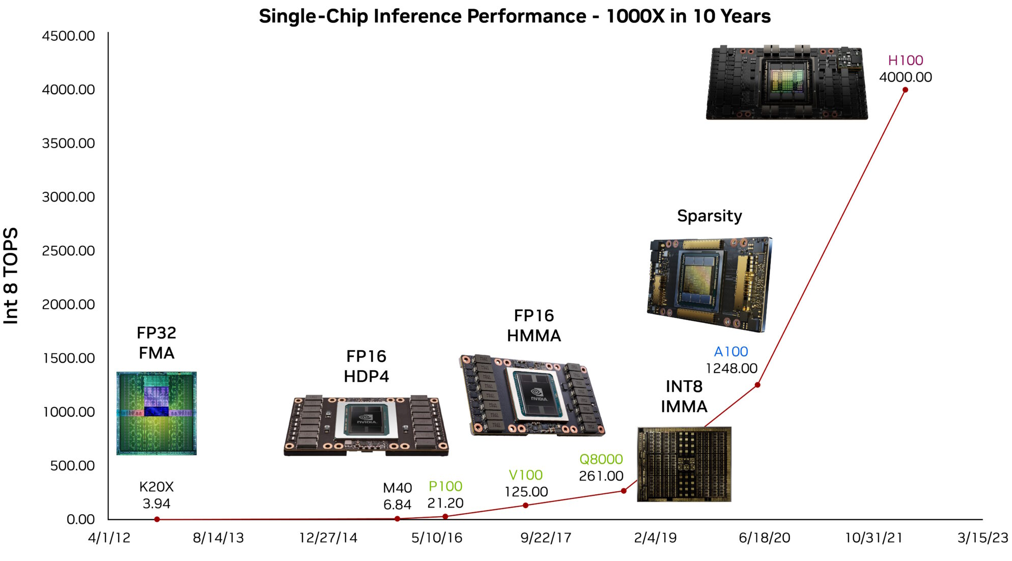](https://mlsysbook.ai/contents/core/hw_acceleration/images/png/int8_tops_nvidia.png "Figure 3: GPU Performance Scaling: NVIDIA GPUs experienced a 10\times increase in integer 8-bit TOPS (tera operations per second) over a decade, driven by architectural innovations transitioning from floating-point to tensor core acceleration. This trend reflects the growing specialization of hardware for deep learning workloads and the increasing demand for efficient inference capabilities.")
Figure 3: **GPU Performance Scaling**: NVIDIA GPUs experienced a \\(10\\times\\) increase in integer 8-bit TOPS (tera operations per second) over a decade, driven by architectural innovations transitioning from floating-point to tensor core acceleration. This trend reflects the growing specialization of hardware for deep learning workloads and the increasing demand for efficient inference capabilities.
#### Processing Elements
The highest level of execution unit organization integrates multiple tensor cores with local memory into processing elements (PEs). A processing element serves as a fundamental building block in many AI accelerators, combining different computational units to efficiently execute neural network operations. Each PE typically includes vector units for element-wise operations, tensor cores for matrix computation, special function units for non-linear transformations, and dedicated memory resources to optimize data locality and minimize data movement overhead.
Processing elements play an essential role in AI hardware by balancing computational density with memory access efficiency. Their design varies across different architectures to support diverse workloads and scalability requirements. Graphcore’s Intelligence Processing Unit (IPU) distributes computation across 1,472 tiles, each containing independent processing elements optimized for fine-grained parallelism ([Graphcore 2020](https://mlsysbook.ai/contents/core/hw_acceleration/hw_acceleration.html#ref-Graphcore2020)
). Cerebras extends this approach in the CS-2 system, integrating 850,000 processing elements across a wafer-scale device to accelerate sparse computations. Tesla’s D1 processor arranges processing elements with substantial local memory, optimizing throughput and latency for real-time autonomous vehicle workloads ([Quinnell 2024](https://mlsysbook.ai/contents/core/hw_acceleration/hw_acceleration.html#ref-Tesla2021)
).
Graphcore. 2020. “The Colossus MK2 IPU Processor.” _Graphcore Technical Paper_.
Quinnell, Eric. 2024. “Tesla Transport Protocol over Ethernet (TTPoE): A New Lossy, Exa-Scale Fabric for the Dojo AI Supercomputer.” In _2024 IEEE Hot Chips 36 Symposium (HCS)_, 1–23. IEEE. [https://doi.org/10.1109/hcs61935.2024.10664947](https://doi.org/10.1109/hcs61935.2024.10664947)
.
Processing elements provide the structural foundation for large-scale AI acceleration. Their efficiency depends not only on computational capability but also on interconnect strategies and memory hierarchy design. The next sections explore how these architectural choices impact performance across different AI workloads.
Tensor processing units have enabled substantial efficiency gains in AI workloads by using hardware-accelerated matrix computation. Their role continues to evolve as architectures incorporate support for advanced execution techniques, including structured sparsity and workload-specific optimizations. The effectiveness of these units, however, depends not only on their computational capabilities but also on how they interact with memory hierarchies and data movement mechanisms, which are examined in subsequent sections.
#### Systolic Arrays
While tensor cores package matrix operations into structured computational units, systolic arrays provide an alternative approach optimized for continuous data flow and operand reuse. The fundamental motivation for systolic architectures stems from the energy efficiency constraints discussed earlier—minimizing the impact of memory access penalties through architectural design. A systolic array arranges processing elements in a grid pattern, where data flows rhythmically between neighboring units in a synchronized manner, enabling each operand to participate in multiple computations as it propagates through the array. This structured movement minimizes external memory accesses by maximizing local data reuse—a single weight value can contribute to dozens of operations as it moves through the processing elements, fundamentally transforming the energy profile from memory-bound to compute-efficient execution.
The concept of systolic arrays was first introduced by Kung and Leiserson[24](https://mlsysbook.ai/contents/core/hw_acceleration/hw_acceleration.html#fn24)
, who formalized their use in parallel computing architectures for efficient matrix operations ([Kung 1982](https://mlsysbook.ai/contents/core/hw_acceleration/hw_acceleration.html#ref-Kung1982)
). Unlike general-purpose execution units, systolic arrays exploit spatial and temporal locality by reusing operands as they propagate through the grid. Google’s TPU exemplifies this architectural approach. In the TPUv4, a \\(128\\times128\\) systolic array of multiply-accumulate units processes matrix operations by streaming data through the array in a pipelined manner, as shown in [Figure 4](https://mlsysbook.ai/contents/core/hw_acceleration/hw_acceleration.html#fig-systolic-array)
.
24 **Systolic Array Renaissance**: H.T. Kung and Charles Leiserson introduced systolic arrays at CMU in 1979 for VLSI signal processing, but the concept languished for decades due to programming complexity. Google’s 2016 TPU resurrection proved these “heartbeat” architectures could deliver massive efficiency gains for neural networks—the TPUv1’s \\(256\\times 256\\) systolic array achieved 92 TOPS for 8-bit integer operations while consuming just 40 watts, making systolic arrays the dominant AI architecture today.
Kung. 1982. “Why Systolic Architectures?” _Computer_ 15 (1): 37–46. [https://doi.org/10.1109/mc.1982.1653825](https://doi.org/10.1109/mc.1982.1653825)
.
The systolic array architecture achieves computational efficiency through synchronized data movement across a structured grid of processing elements. Systolic arrays organize computation around four fundamental components:
1. **Control Unit**: Coordinates timing and data distribution across the array, maintaining synchronized operation throughout the computational grid
2. Data Streams: Input matrices propagate through coordinated pathways—matrix A elements traverse horizontally while matrix B elements flow vertically through the processing grid
3. **Processing Element Grid**: Individual processing elements execute multiply-accumulate operations on streaming data, generating partial results that accumulate toward the final computation
4. **Output Collection**: Results aggregate at designated output boundaries where accumulated partial sums form complete matrix elements
The synchronized data flow ensures that matrix element A\[i,k\] encounters corresponding B\[k,j\] elements at precise temporal intervals, executing the multiply-accumulate operations required for matrix multiplication C\[i,j\] = Σ A\[i,k\] × B\[k,j\]. This systematic reuse of operands across multiple processing elements substantially reduces memory bandwidth requirements by eliminating redundant data fetches from external memory subsystems.
Consider the multiplication of 2×2 matrices A and B within a systolic array. During the first computational cycle, element A\[0,0\]=2 propagates horizontally while B\[0,0\]=1 moves vertically, converging at processing element PE(0,0) to execute the multiplication 2×1=2. In the subsequent cycle, the same A\[0,0\]=2 advances to PE(0,1) where it encounters B\[0,1\]=3, computing 2×3=6. Concurrently, A\[0,1\]=4 enters PE(0,0) to engage with the next B matrix element. This coordinated data movement enables systematic operand reuse across multiple computational operations, eliminating redundant memory accesses and exemplifying the fundamental efficiency principle underlying systolic array architectures.
[](https://mlsysbook.ai/contents/core/hw_acceleration/39ea304c244f2c4267e1f8d4d12d87e8b95dee80.svg "Figure 4: Systolic Array Dataflow: Processing elements within the array execute matrix operations by streaming data in a pipelined manner, maximizing operand reuse and minimizing memory access compared to traditional memory-compute architectures. This spatial and temporal locality enables efficient parallel computation, as exemplified by the multiply-accumulate units in Google’s tpuv4.")
Figure 4: **Systolic Array Dataflow**: Processing elements within the array execute matrix operations by streaming data in a pipelined manner, maximizing operand reuse and minimizing memory access compared to traditional memory-compute architectures. This spatial and temporal locality enables efficient parallel computation, as exemplified by the multiply-accumulate units in Google’s tpuv4.
Each processing element in the array performs a multiply-accumulate operation in every cycle:
1. Receives an input activation from above
2. Receives a weight value from the left
3. Multiplies these values and adds to its running sum
4. Passes the input activation downward and the weight value rightward to neighboring elements
This structured computation model minimizes data movement between global memory and processing elements, improving both efficiency and scalability. As systolic arrays operate in a streaming fashion, they are particularly effective for high-throughput workloads such as deep learning training and inference.
While the diagram in [Figure 4](https://mlsysbook.ai/contents/core/hw_acceleration/hw_acceleration.html#fig-systolic-array)
illustrates one common systolic array implementation, systolic architectures vary significantly across different accelerator designs. Training-focused architectures like Google’s TPU employ large arrays optimized for high computational throughput, while inference-oriented designs found in edge devices prioritize energy efficiency with smaller configurations.
The fundamental principle remains consistent: data flows systematically through processing elements, with inputs moving horizontally and vertically to compute partial sums in a synchronized fashion. However, as detailed in [Section 1.4.1](https://mlsysbook.ai/contents/core/hw_acceleration/hw_acceleration.html#sec-ai-acceleration-understanding-ai-memory-wall-3ea9)
, practical effectiveness is ultimately constrained by memory bandwidth bottlenecks.
A 128×128 systolic array capable of 16,384 operations per cycle requires continuous data feed to maintain utilization—each cycle demands fresh input activations and weight parameters that must traverse from off-chip memory through on-chip buffers to the array edges. The TPU’s 1,200 GB/s on-chip bandwidth enables high utilization, but even this substantial bandwidth becomes limiting when processing large transformer models where memory requirements exceed on-chip capacity.
Recall from **[Chapter 10: Model Optimizations](https://mlsysbook.ai/contents/core/optimizations/optimizations.html#sec-model-optimizations)
** that quantization reduces model memory footprint by converting FP32 weights to INT8 representations—this optimization directly addresses the memory bandwidth constraints identified here. Converting 32-bit floating-point weights to 8-bit integers reduces memory traffic by 4×, transforming bandwidth-bound operations into compute-bound workloads where systolic arrays can achieve higher utilization. Similarly, structured pruning removes entire rows or columns of weight matrices, reducing both the data volume that must traverse memory hierarchies and the computation required. These algorithmic optimizations prove valuable precisely because they target the memory bottleneck that limits accelerator performance in practice.
#### Numerics in AI Acceleration
The efficiency of AI accelerators is not determined by computational power alone but also by the precision of numerical representations. The choice of numerical format shapes the balance between accuracy, throughput, and energy consumption, influencing how different execution units, such as SIMD and SIMT units, tensor cores, and systolic arrays, are designed and deployed.
##### Precision Trade-offs
Numerical precision represents a critical design parameter in modern AI accelerators. While higher precision formats provide mathematical stability and accuracy, they come with substantial costs in terms of power consumption, memory bandwidth, and computational throughput. Finding the optimal precision point has become a central challenge in AI hardware architecture.
Early deep learning models primarily relied on single-precision floating point (FP32) for both training and inference. While FP32 offers sufficient dynamic range and precision for stable learning, it imposes high computational and memory costs, limiting efficiency, especially as model sizes increase. Over time, hardware architectures evolved to support lower precision formats such as half-precision floating point (FP16) and bfloat16 (BF16), which reduce memory usage and increase computational throughput while maintaining sufficient accuracy for deep learning tasks. More recently, integer formats (INT8, INT4) have gained prominence in inference workloads, where small numerical representations significantly improve energy efficiency without compromising model accuracy beyond acceptable limits.
The transition from high-precision to lower-precision formats is deeply integrated into hardware execution models. As detailed in [Section 1.3.4.2](https://mlsysbook.ai/contents/core/hw_acceleration/hw_acceleration.html#sec-ai-acceleration-evolution-simd-simt-architectures-e1fd)
, SIMD and SIMT units provide flexible support for multiple precisions. Tensor cores ([Section 1.3.4.3](https://mlsysbook.ai/contents/core/hw_acceleration/hw_acceleration.html#sec-ai-acceleration-tensor-cores-771f)
) accelerate computation using reduced-precision arithmetic, while systolic arrays ([Section 1.3.4.5](https://mlsysbook.ai/contents/core/hw_acceleration/hw_acceleration.html#sec-ai-acceleration-systolic-arrays-6fa8)
) optimize performance by minimizing memory bandwidth constraints through low-precision formats that maximize operand reuse.
Despite the advantages of reduced precision, deep learning models cannot always rely solely on low-bit representations. To address this challenge, modern AI accelerators implement mixed-precision computing, where different numerical formats are used at different stages of execution. These precision choices have important implications for model fairness and reliability. For example, matrix multiplications may be performed in FP16 or BF16, while accumulations are maintained in FP32 to prevent precision loss. Similarly, inference engines leverage INT8 arithmetic while preserving key activations in higher precision when necessary.
##### Mixed-Precision Computing
Modern AI accelerators increasingly support mixed-precision execution, allowing different numerical formats to be used at various stages of computation. Training workloads often leverage FP16 or BF16 for matrix multiplications, while maintaining FP32 accumulations to preserve precision. Inference workloads, by contrast, optimize for INT8 or even INT4, achieving high efficiency while retaining acceptable accuracy.
This shift toward precision diversity is evident in the evolution of AI hardware. Early architectures such as NVIDIA Volta provided limited support for lower precision beyond FP16, whereas later architectures, including Turing and Ampere, expanded the range of supported formats. Ampere GPUs introduced TF32 as a hybrid between FP32 and FP16, alongside broader support for BF16, INT8, and INT4. [Table 5](https://mlsysbook.ai/contents/core/hw_acceleration/hw_acceleration.html#tbl-nvidia-numerics)
illustrates this trend.
Table 5: **Precision Support Evolution**: GPU architectures progressively expanded support for lower-precision data types, enabling performance gains and efficiency improvements in AI workloads. Early architectures primarily utilized FP32, while later generations incorporated FP16, BF16, INT8, and INT4 to accelerate both training and inference tasks.
| | | | |
| --- | --- | --- | --- |
| **Volta** | 2017 | FP16 | FP64, FP32, FP16 |
| **Turing** | 2018 | FP16, INT8 | FP64, FP32, FP16, INT8 |
| **Ampere** | 2020 | FP64, TF32, bfloat16, FP16, INT8, INT4 | FP64, FP32, FP16, bfloat16, INT8 |
[Table 5](https://mlsysbook.ai/contents/core/hw_acceleration/hw_acceleration.html#tbl-nvidia-numerics)
highlights how newer architectures incorporate a growing diversity of numerical formats, reflecting the need for greater flexibility across different AI workloads. This trend suggests that future AI accelerators will continue expanding support for adaptive precision, optimizing both computational efficiency and model accuracy.
The precision format used in hardware design has far-reaching implications. By adopting lower-precision formats, the data transferred between execution units and memory is reduced, leading to decreased memory bandwidth requirements and storage. Tensor cores and systolic arrays can process more lower-precision elements in parallel, thereby increasing the effective throughput in terms of FLOPs. Energy efficiency is also improved, as integer-based computations (e.g., INT8) require lower power compared to floating-point arithmetic—a clear advantage for inference workloads.
As AI models continue to scale in size, accelerator architectures are evolving to support more efficient numerical formats. Future designs are expected to incorporate adaptive precision techniques, dynamically adjusting computation precision based on workload characteristics. This evolution promises further optimization of deep learning performance while striking an optimal balance between accuracy and energy efficiency.
#### Architectural Integration
The organization of computational primitives into execution units determines the efficiency of AI accelerators. While SIMD, tensor cores, and systolic arrays serve as fundamental building blocks, their integration into full-chip architectures varies significantly across different AI processors. The choice of execution units, their numerical precision support, and their connectivity impact how effectively hardware can scale for deep learning workloads.
Modern AI processors exhibit a range of design trade-offs based on their intended applications. Some architectures, such as NVIDIA’s A100, integrate large numbers of tensor cores optimized for FP16-based training, while Google’s TPUv4 prioritizes high-throughput BF16 matrix multiplications. Inference-focused processors, such as Intel’s Sapphire Rapids, incorporate INT8-optimized tensor cores to maximize efficiency. The Apple M1, designed for mobile workloads, employs smaller processing elements optimized for low-power FP16 execution. These design choices reflect the growing flexibility in numerical precision and execution unit organization, as discussed in the previous section.
[Table 6](https://mlsysbook.ai/contents/core/hw_acceleration/hw_acceleration.html#tbl-execution-units)
summarizes the execution unit configurations across contemporary AI processors.
Table 6: **AI Processor Configurations**: Modern AI processors prioritize different execution unit characteristics to optimize performance for specific workloads; NVIDIA A100 leverages wide SIMD and tensor cores for training, Google TPUv4 emphasizes high-throughput BF16 matrix multiplication, and Intel Sapphire Rapids focuses on INT8-optimized inference, while apple M1 prioritizes low-power FP16 execution on smaller processing elements. These variations in SIMD width, tensor core size, and processing element count reflect the growing diversity in AI hardware architectures and their targeted applications.
| | | | | |
| --- | --- | --- | --- | --- |
| **NVIDIA A100** | 1024-bit | \\(4\\times4\\times4\\) FP16 | 108 SMs | Training, HPC |
| **Google TPUv4** | 128-wide | \\(128\\times128\\) BF16 | 2 cores/chip | Training |
| **Intel Sapphire** | 512-bit AVX | \\(32\\times32\\) INT8/BF16 | 56 cores | Inference |
| **Apple M1** | 128-bit NEON | \\(16\\times16\\) FP16 | 8 NPU cores | Mobile inference |
[Table 6](https://mlsysbook.ai/contents/core/hw_acceleration/hw_acceleration.html#tbl-execution-units)
highlights how execution unit configurations vary across architectures to optimize for different deep learning workloads. Training accelerators prioritize high-throughput floating-point tensor operations, whereas inference processors focus on low-precision integer execution for efficiency. Meanwhile, mobile accelerators balance precision and power efficiency to meet real-time constraints.
### Cost-Performance Analysis
While architectural specifications define computational potential, practical deployment decisions require understanding cost-performance trade-offs across different accelerator options. However, raw computational metrics alone provide an incomplete picture—the fundamental constraint in modern AI acceleration is not compute capacity but data movement efficiency.
The energy differential established earlier—where memory access costs dominate computation—drives the entire specialized hardware revolution. This disparity explains why GPUs with high memory bandwidth achieve 40-60% utilization, while TPUs with systolic arrays achieve 85% utilization by minimizing data movement.
[Table 7](https://mlsysbook.ai/contents/core/hw_acceleration/hw_acceleration.html#tbl-accelerator-economics)
provides concrete cost-performance data for representative accelerators, but the economic analysis must account for utilization efficiency and energy consumption patterns that determine real-world performance.
Table 7: **Accelerator Cost-Performance Comparison**: Hardware costs must be evaluated against computational capabilities to determine optimal deployment strategies. While newer accelerators like H100 offer better price-performance ratios, total cost of ownership includes power consumption, cooling requirements, and infrastructure costs that significantly impact operational economics. \*TPU pricing estimated from cloud rates.
| | | | | |
| --- | --- | --- | --- | --- |
| **NVIDIA V100** | ~$9,000 (2017-19) | 125 TFLOPS | 900 GB/s | $72/TFLOP |
| **NVIDIA A100** | $15,000 | 312 TFLOPS (FP16) | 1,935 GB/s | $48/TFLOP |
| **NVIDIA H100** | $25,000-30,000 | 756 TFLOPS (TF32) | 3,350 GB/s | $33/TFLOP |
| **Google TPUv4** | ~$8,000\* | 275 TFLOPS (BF16) | 1,200 GB/s | $29/TFLOP |
| **Intel H100** | $12,000 | 200 TFLOPS (INT8) | 800 GB/s | $60/TFLOP |
A startup training large language models faces the choice between 8 V100s ($72K) providing 1,000 TFLOPS or 4 A100s ($60K) delivering 1,248 TFLOPS. However, performance analysis reveals the true performance story—transformer training with its arithmetic intensity of 0.5-2 FLOPS/byte makes both configurations memory-bandwidth bound rather than compute-bound. The A100’s 1,935 GB/s bandwidth delivers 2.15× higher sustainable performance than V100’s 900 GB/s, making the effective performance gain 115% rather than the 25% suggested by peak FLOPS. When combined with 17% lower hardware cost and 30% better energy efficiency (400 W vs 300 W per effective TFLOP), the A100 configuration provides compelling economic advantages that compound over multi-year deployments.
These cost dynamics explain the rapid adoption of newer accelerators despite higher unit prices. The H100’s $33/TFLOP represents a 54% improvement over V100’s $72/TFLOP, but more importantly, its 3,350 GB/s bandwidth enables 3.7× higher memory throughput per dollar—the metric that determines real-world transformer performance. Cloud deployment further complicates the analysis, as providers typically charge $2-4/hour for high-end accelerators, making the break-even point between purchase and rental highly dependent on utilization patterns and energy costs that can account for 60-70% of total operational expenses over a three-year lifecycle.
Framework selection significantly impacts these economic decisions—detailed hardware-framework optimization strategies are covered in **[Chapter 7: AI Frameworks](https://mlsysbook.ai/contents/core/frameworks/frameworks.html#sec-ai-frameworks)
**, while performance evaluation methodologies are discussed in **[Chapter 12: Benchmarking AI](https://mlsysbook.ai/contents/core/benchmarking/benchmarking.html#sec-benchmarking-ai)
**.
While execution units define the compute potential of an accelerator, their effectiveness is fundamentally constrained by data movement and memory hierarchy. Achieving high utilization of compute resources requires efficient memory systems that minimize data transfer overhead and optimize locality. Understanding these constraints reveals why memory architecture becomes as critical as computational design in AI acceleration.
**Self-Check: Question 1.3**
1. What is the primary role of AI compute primitives in neural network execution?
1. To optimize the execution of core computational patterns in neural networks
2. To provide a high-level programming interface for machine learning frameworks
3. To replace general-purpose CPUs in all computing tasks
4. To ensure compatibility across different neural network architectures
2. Explain how vector operations enhance the efficiency of neural network computations in AI accelerators.
3. The hardware component that performs non-linear transformations like ReLU and sigmoid in a single cycle is known as the \_\_\_\_.
4. Order the following computational steps for executing a dense layer in a neural network: (1) Apply activation function, (2) Multiply inputs by weights, (3) Add bias.
5. Which of the following is NOT a characteristic of AI compute primitives?
1. They are frequently used in neural network computations.
2. They offer significant energy efficiency gains.
3. They are designed to replace all general-purpose computing tasks.
4. They remain stable across different neural network architectures.
[See Answers →](https://mlsysbook.ai/contents/core/hw_acceleration/hw_acceleration.html#quiz-answer-sec-ai-acceleration-ai-compute-primitives-8471)
AI Memory Systems
-----------------
The execution units examined in previous sections—SIMD units, tensor cores, and systolic arrays—provide impressive computational throughput: modern accelerators achieve 100 to 1000 TFLOPS for neural network operations. Yet these theoretical capabilities remain unrealized in practice when memory subsystems cannot supply data at sufficient rates. This fundamental constraint, termed the AI memory wall, represents the dominant bottleneck in real-world accelerator performance.
Unlike conventional workloads, ML models require frequent access to large volumes of parameters, activations, and intermediate results, leading to substantial memory bandwidth demands—a challenge that intersects with the data management strategies covered in **[Chapter 6: Data Engineering](https://mlsysbook.ai/contents/core/data_engineering/data_engineering.html#sec-data-engineering)
**. Modern AI hardware addresses these challenges through advanced memory hierarchies, efficient data movement techniques, and compression strategies that promote efficient execution and improved AI acceleration.
This section examines memory system design through four interconnected perspectives. First, we quantify the growing disparity between computational throughput and memory bandwidth, revealing why the AI memory wall represents the dominant performance constraint in modern accelerators. Second, we explore how memory hierarchies balance competing demands for speed, capacity, and energy efficiency through carefully structured tiers from on-chip SRAM to off-chip DRAM. Third, we analyze communication patterns between host systems and accelerators, exposing transfer bottlenecks that limit end-to-end performance. Finally, we examine how different neural network architectures—multilayer perceptrons, convolutional networks, and transformers—create distinct memory pressure patterns that inform hardware design decisions and optimization strategies.
### Understanding the AI Memory Wall
The AI memory wall represents the fundamental bottleneck constraining modern accelerator performance—the growing disparity between computational throughput and memory bandwidth that prevents accelerators from achieving their theoretical capabilities. While compute units can execute millions of operations per second through specialized primitives like vector operations and matrix multiplications, they depend entirely on memory systems to supply the continuous stream of weights, activations, and intermediate results these operations require.
#### Quantifying the Compute-Memory Performance Gap
The severity of this constraint becomes apparent when examining scaling trends. Over the past 20 years, peak computational capabilities have scaled at 3.0× every two years, while DRAM bandwidth has grown at only 1.6× during the same period ([Gholami et al. 2024](https://mlsysbook.ai/contents/core/hw_acceleration/hw_acceleration.html#ref-gholami2024ai)
). This divergence creates an exponentially widening gap where accelerators possess massive computational power but cannot access data quickly enough to utilize it. Modern hardware exemplifies this imbalance: an NVIDIA H100 delivers 989 TFLOPS but only 3.35 TB/s memory bandwidth ([Choquette 2023](https://mlsysbook.ai/contents/core/hw_acceleration/hw_acceleration.html#ref-nvidia2022h100)
), requiring 295 operations per byte to achieve full utilization—far exceeding the 1-10 operations per byte typical in neural networks.
Gholami, Amir, Zhewei Yao, Sehoon Kim, Coleman Hooper, Michael W. Mahoney, and Kurt Keutzer. 2024. “AI and Memory Wall.” _IEEE Micro_ 44 (3): 33–39. [https://doi.org/10.1109/mm.2024.3373763](https://doi.org/10.1109/mm.2024.3373763)
.
The memory wall manifests through three critical constraints. First, the energy disparity—accessing DRAM consumes 640 pJ compared to 3.7 pJ for computation ([Horowitz 2014](https://mlsysbook.ai/contents/core/hw_acceleration/hw_acceleration.html#ref-Horowitz2014)
), creating a 173× energy penalty that often limits performance due to power budgets rather than computational capacity. Second, the bandwidth limitation—even TB/s memory systems cannot feed thousands of parallel compute units continuously, forcing 50-70% idle time in typical workloads. Third, the latency hierarchy—off-chip memory access requires hundreds of cycles, creating pipeline stalls that cascade through parallel execution units.
As illustrated in [Figure 5](https://mlsysbook.ai/contents/core/hw_acceleration/hw_acceleration.html#fig-compute-memory-imbalance)
, this “AI Memory Wall” continues to widen, making memory bandwidth rather than compute the primary constraint in AI acceleration.
[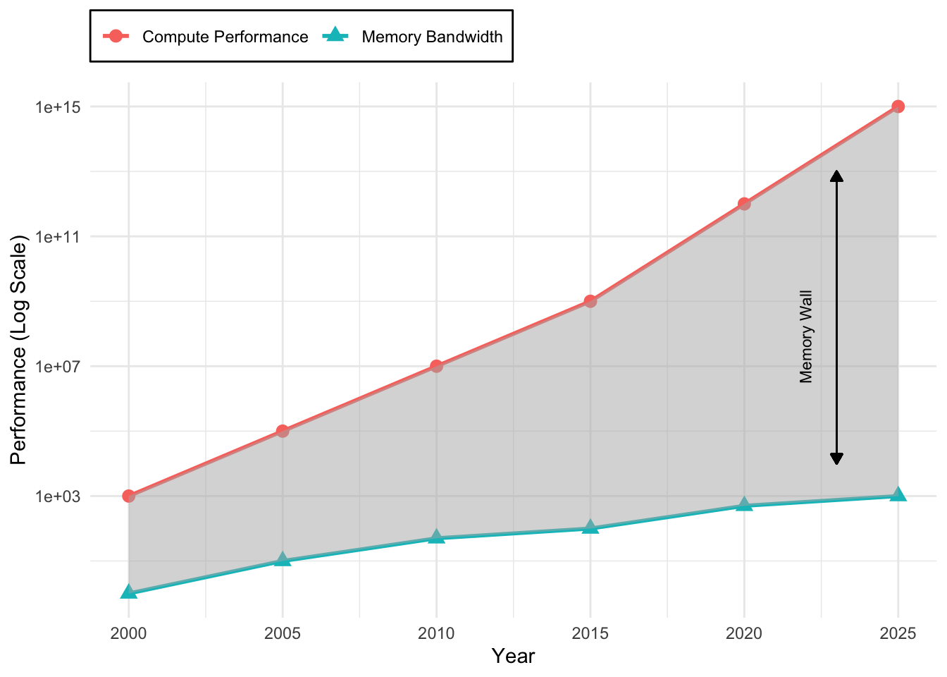](https://mlsysbook.ai/contents/core/hw_acceleration/hw_acceleration_files/figure-html/fig-compute-memory-imbalance-1.png "Figure 5: AI Memory Wall: The growing disparity between compute performance and memory bandwidth emphasizes the increasing challenge in sustaining peak computational efficiency due to memory constraints. Over the past 20 years, while computational capabilities have advanced rapidly, memory bandwidth has not kept pace, leading to potential bottlenecks in data-intensive applications.")
Figure 5: **AI Memory Wall**: The growing disparity between compute performance and memory bandwidth emphasizes the increasing challenge in sustaining peak computational efficiency due to memory constraints. Over the past 20 years, while computational capabilities have advanced rapidly, memory bandwidth has not kept pace, leading to potential bottlenecks in data-intensive applications.
Beyond performance limitations, memory access imposes a significant energy cost. Fetching data from off-chip DRAM consumes far more energy than performing arithmetic operations ([Horowitz 2014](https://mlsysbook.ai/contents/core/hw_acceleration/hw_acceleration.html#ref-Horowitz2014)
). This inefficiency is particularly evident in machine learning models, where large parameter sizes, frequent memory accesses, and non-uniform data movement patterns exacerbate memory bottlenecks. The energy differential drives architectural decisions—Google’s TPU achieves 30-83\\(\\times\\) better energy efficiency than contemporary GPUs by minimizing data movement through systolic arrays and large on-chip memory. These design choices demonstrate that energy constraints, not computational limits, often determine practical deployment feasibility.
Horowitz, Mark. 2014. “1.1 Computing’s Energy Problem (and What We Can Do about It).” In _2014 IEEE International Solid-State Circuits Conference Digest of Technical Papers (ISSCC)_. IEEE. [https://doi.org/10.1109/isscc.2014.6757323](https://doi.org/10.1109/isscc.2014.6757323)
.
#### Memory Access Patterns in ML Workloads
Machine learning workloads place substantial demands on memory systems due to the large volume of data involved in computation. Unlike traditional compute-bound applications, where performance is often dictated by the speed of arithmetic operations, ML workloads are characterized by high data movement requirements. The efficiency of an accelerator is not solely determined by its computational throughput but also by its ability to continuously supply data to processing units without introducing stalls or delays.
A neural network processes multiple types of data throughout its execution, each with distinct memory access patterns:
* **Model parameters (weights and biases)**: Machine learning models, particularly those used in large-scale applications such as natural language processing and computer vision, often contain millions to billions of parameters. Storing and accessing these weights efficiently is essential for maintaining throughput.
* **Intermediate activations**: During both training and inference, each layer produces intermediate results that must be temporarily stored and retrieved for subsequent operations. These activations can contribute significantly to memory overhead, particularly in deep architectures.
* **Gradients (during training)**: Backpropagation requires storing and accessing gradients for every parameter, further increasing the volume of data movement between compute units and memory.
As models increase in size and complexity, improvements in memory capacity and bandwidth become essential. Although specialized compute units accelerate operations like matrix multiplications, their overall performance depends on the continuous, efficient delivery of data to the processing elements. In large-scale applications, such as natural language processing and computer vision, models often incorporate millions to billions of parameters ([Brown et al. 2020](https://mlsysbook.ai/contents/core/hw_acceleration/hw_acceleration.html#ref-Brown2020)
). Consequently, achieving high performance necessitates minimizing delays and stalls caused by inefficient data movement between memory and compute units ([Narayanan et al. 2021](https://mlsysbook.ai/contents/core/hw_acceleration/hw_acceleration.html#ref-Narayanan2021)
; [Xingyu 2019](https://mlsysbook.ai/contents/core/hw_acceleration/hw_acceleration.html#ref-Huang2019)
).
Xingyu, Huang et al. 2019. “Addressing the Memory Bottleneck in AI Accelerators.” _IEEE Micro_.
One way to quantify this challenge is by comparing the data transfer time with the time required for computations. Specifically, we define the memory transfer time as \\\[ T\_{\\text{mem}} = \\frac{M\_{\\text{total}}}{B\_{\\text{mem}}}, \\\] where \\(M\_{\\text{total}}\\) is the total data volume and \\(B\_{\\text{mem}}\\) is the available memory bandwidth. In contrast, the compute time is given by \\\[ T\_{\\text{compute}} = \\frac{\\text{FLOPs}}{P\_{\\text{peak}}}, \\\] with the number of floating-point operations (FLOPs) divided by the peak hardware throughput, \\(P\_{\\text{peak}}\\). When \\(T\_{\\text{mem}} > T\_{\\text{compute}}\\), the system becomes memory-bound, meaning that the processing elements spend more time waiting for data than performing computations. This imbalance demonstrates the need for memory-optimized architectures and efficient data movement strategies to sustain high performance.
[Figure 6](https://mlsysbook.ai/contents/core/hw_acceleration/hw_acceleration.html#fig-memory-wall)
demonstrates the emerging challenge between model growth and hardware memory capabilities, illustrating the “AI Memory Wall.” The figure tracks AI model sizes (red dots) and hardware memory bandwidth (blue dots) over time on a log scale. Model parameters have grown exponentially, from AlexNet’s ~62.3M parameters in 2012 to Gemini 1’s trillion-scale parameters in 2023, as shown by the steeper red trend line. In contrast, hardware memory bandwidth, represented by successive generations of NVIDIA GPUs (~100-200 GB/s) and Google TPUs (~2-3 TB/s), has increased more gradually (blue trend line). The expanding shaded region between these trends corresponds to the “AI Memory Wall,” which will be an architectural challenge where model scaling outpaces available memory bandwidth. This growing disparity necessitates increasingly sophisticated memory management and model optimization techniques to maintain computational efficiency.
#### Irregular Memory Access
Unlike traditional computing workloads, where memory access follows well-structured and predictable patterns, machine learning models often exhibit irregular memory access behaviors that make efficient data retrieval a challenge. These irregularities arise due to the nature of ML computations, where memory access patterns are influenced by factors such as batch size, layer type, and sparsity. As a result, standard caching mechanisms and memory hierarchies often struggle to optimize performance, leading to increased memory latency and inefficient bandwidth utilization.
[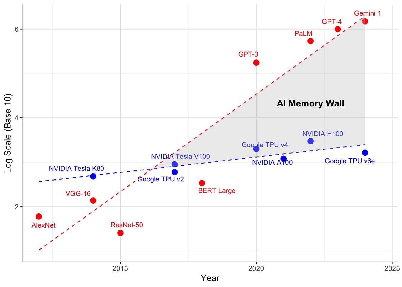](https://mlsysbook.ai/contents/core/hw_acceleration/hw_acceleration_files/figure-html/fig-memory-wall-1.png "Figure 6: AI Memory Wall: The figure emphasizes the growing disparity between model sizes and hardware memory bandwidths, illustrating the challenge in sustaining performance as models become more complex.")
Figure 6: **AI Memory Wall**: The figure emphasizes the growing disparity between model sizes and hardware memory bandwidths, illustrating the challenge in sustaining performance as models become more complex.
To better understand how ML workloads differ from traditional computing workloads, it is useful to compare their respective memory access patterns ([Table 8](https://mlsysbook.ai/contents/core/hw_acceleration/hw_acceleration.html#tbl-traditional-vs-ml-mem)
). Traditional workloads, such as scientific computing, general-purpose CPU applications, and database processing, typically exhibit well-defined memory access characteristics that benefit from standard caching and prefetching techniques. ML workloads, on the other hand, introduce highly dynamic access patterns that challenge conventional memory optimization strategies.
One key source of irregularity in ML workloads stems from batch size and execution order. The way input data is processed in batches directly affects memory reuse, creating a complex optimization challenge. Small batch sizes decrease the likelihood of reusing cached activations and weights, resulting in frequent memory fetches from slower, off-chip memory. Larger batch sizes can improve reuse and amortize memory access costs, but simultaneously place higher demands on available memory bandwidth, potentially creating congestion at different memory hierarchy levels. This delicate balance requires careful consideration of model architecture and available hardware resources.
Table 8: **Memory Access Characteristics**: Traditional workloads exhibit predictable, sequential memory access, benefiting from standard caching, while machine learning workloads introduce irregular and dynamic patterns due to sparsity and data dependencies that challenge conventional memory optimization techniques. Understanding these differences is crucial for designing memory systems that efficiently support the unique demands of modern AI applications.
| | | |
| --- | --- | --- |
| **Memory Access Pattern** | Regular and predictable (e.g., sequential reads, structured patterns) | Irregular and dynamic (e.g., sparsity, attention mechanisms) |
| **Cache Locality** | High temporal and spatial locality | Often low locality, especially in large models |
| **Data Reuse** | Structured loops with frequent data reuse | Sparse and dynamic reuse depending on layer type |
| **Data Dependencies** | Well-defined dependencies allow efficient prefetching | Variable dependencies based on network structure |
| **Workload Example** | Scientific computing (e.g., matrix factorizations, physics simulations) | Neural networks (e.g., CNNs, Transformers, sparse models) |
| **Memory Bottleneck** | DRAM latency, cache misses | Off-chip bandwidth constraints, memory fragmentation |
| **Impact on Energy Consumption** | Moderate, driven by FLOP-heavy execution | High, dominated by data movement costs |
Different neural network layers interact with memory in distinct ways beyond batch size considerations. Convolutional layers benefit from spatial locality, as neighboring pixels in an image are processed together, enabling efficient caching of small weight kernels. Conversely, fully connected layers require frequent access to large weight matrices, often leading to more randomized memory access patterns that poorly align with standard caching policies. Transformers introduce additional complexity, as attention mechanisms demand accessing large key-value pairs stored across varied memory locations. The dynamic nature of sequence length and attention span renders traditional prefetching strategies ineffective, resulting in unpredictable memory latencies.
Another significant factor contributing to irregular memory access is sparsity[25](https://mlsysbook.ai/contents/core/hw_acceleration/hw_acceleration.html#fn25)
in neural networks. Many modern ML models employ techniques such as weight pruning, activation sparsity, and structured sparsity to reduce computational overhead. However, these optimizations often lead to non-uniform memory access, as sparse representations necessitate fetching scattered elements rather than sequential blocks, making hardware caching less effective. Models that incorporate dynamic computation paths, such as Mixture of Experts and Adaptive Computation Time, introduce highly non-deterministic memory access patterns, where the active neurons or model components can vary with each inference step. This variability challenges efficient prefetching and caching strategies.
25 **Sparsity in Neural Networks**: The property that most weights or activations in a neural network are zero or near-zero, enabling computational and memory optimizations. Natural sparsity occurs when ReLU activations zero out 50-90% of values, while artificial sparsity results from pruning techniques that remove 90-99% of weights with minimal accuracy loss. Sparse networks can be 10-100\\(\\times\\) smaller and faster, but require specialized hardware support (like NVIDIA’s 2:4 sparsity in A100) or software optimization to realize benefits, as standard dense hardware performs zero multiplications inefficiently.
These irregularities have significant consequences. ML workloads often experience reduced cache efficiency, as activations and weights may not be accessed in predictable sequences. This leads to increased reliance on off-chip memory traffic, which slows down execution and consumes more energy. Irregular access patterns contribute to memory fragmentation, where the way data is allocated and retrieved results in inefficient utilization of available memory resources. The combined effect is that ML accelerators frequently encounter memory bottlenecks that limit their ability to fully utilize available compute power.
### Memory Hierarchy
To address the memory challenges in ML acceleration, hardware designers implement sophisticated memory hierarchies that balance speed, capacity, and energy efficiency. Understanding this hierarchy is essential before examining how different ML architectures utilize memory resources. Unlike general-purpose computing, where memory access patterns are often unpredictable, ML workloads exhibit structured reuse patterns that can be optimized through careful organization of data across multiple memory levels.
At the highest level, large-capacity but slow storage devices provide long-term model storage. At the lowest level, high-speed registers and caches ensure that compute units can access operands with minimal latency. Between these extremes, intermediate memory levels, such as scratchpad memory, high-bandwidth memory, and off-chip DRAM, offer trade-offs between performance and capacity.
[Table 9](https://mlsysbook.ai/contents/core/hw_acceleration/hw_acceleration.html#tbl-memory-heirarchy)
summarizes the key characteristics of different memory levels in modern AI accelerators. Each level in the hierarchy has distinct latency, bandwidth, and capacity properties, which directly influence how neural network data, such as weights, activations, and intermediate results, should be allocated.
Table 9: **Memory Hierarchy Trade-Offs**: AI accelerators leverage a multi-level memory hierarchy to balance performance and capacity, optimizing data access for computationally intensive machine learning tasks. Each level provides distinct latency, bandwidth, and capacity characteristics that dictate how neural network components—weights, activations, and intermediate results—should be strategically allocated to minimize bottlenecks and maximize throughput.
| | | | | |
| --- | --- | --- | --- | --- |
| **Registers** | ~1 cycle | Highest | Few values | Storing operands for immediate computation |
| **L1/L2 Cache (SRAM)** | ~1-10 ns | High | KBs-MBs | Caching frequently accessed activations and small weight blocks |
| **Scratchpad Memory** | ~5-20 ns | High | MBs | Software-managed storage for intermediate computations |
| **High-Bandwidth Memory (HBM)** | ~100 ns | Very High | GBs | Storing large model parameters and activations for high-speed access |
| **Off-Chip DRAM (DDR, GDDR, LPDDR)** | ~50-150 ns | Moderate | GBs-TBs | Storing entire model weights that do not fit on-chip |
| **Flash Storage (SSD/NVMe)** | ~100 µs - 1 ms | Low | TBs | Storing pre-trained models and checkpoints for later loading |
#### On-Chip Memory
Each level of the memory hierarchy serves a distinct role in AI acceleration, with different trade-offs in speed, capacity, and accessibility. Registers, located within compute cores, provide the fastest access but can only store a few operands at a time. These are best utilized for immediate computations, where the operands needed for an operation can be loaded and consumed within a few cycles. However, because register storage is so limited, frequent memory accesses are required to fetch new operands and store intermediate results.
To reduce the need for constant data movement between registers and external memory, small but fast caches serve as an intermediary buffer. These caches store recently accessed activations, weights, and intermediate values, ensuring that frequently used data remains available with minimal delay. However, the size of caches is limited, making them insufficient for storing full feature maps or large weight tensors in machine learning models. As a result, only the most frequently used portions of a model’s parameters or activations can reside here at any given time.
For larger working datasets, many AI accelerators include scratchpad memory, which offers more storage than caches but with a crucial difference: it allows explicit software control over what data is stored and when it is evicted. Unlike caches, which rely on hardware-based eviction policies, scratchpad memory enables machine learning workloads to retain key values such as activations and filter weights for multiple layers of computation. This capability is particularly useful in models like convolutional neural networks, where the same input feature maps and filter weights are reused across multiple operations. By keeping this data in scratchpad memory rather than reloading it from external memory, accelerators can significantly reduce unnecessary memory transfers and improve overall efficiency ([Chen, Emer, and Sze 2017](https://mlsysbook.ai/contents/core/hw_acceleration/hw_acceleration.html#ref-Chen2016)
).
#### Off-Chip Memory
Beyond on-chip memory, high-bandwidth memory provides rapid access to larger model parameters and activations that do not fit within caches or scratchpad buffers. HBM achieves its high performance by stacking multiple memory dies and using wide memory interfaces, allowing it to transfer large amounts of data with minimal latency compared to traditional DRAM. Because of its high bandwidth and lower latency, HBM is often used to store entire layers of machine learning models that must be accessed quickly during execution. However, its cost and power consumption limit its use primarily to high-performance AI accelerators, making it less common in power-constrained environments such as edge devices.
When a machine learning model exceeds the capacity of on-chip memory and HBM, it must rely on off-chip DRAM, such as DDR, GDDR, or LPDDR. While DRAM offers significantly greater storage capacity, its access latency is higher, meaning that frequent retrievals from DRAM can introduce execution bottlenecks. To make effective use of DRAM, models must be structured so that only the necessary portions of weights and activations are retrieved at any given time, minimizing the impact of long memory fetch times.
At the highest level of the hierarchy, flash storage and solid-state drives (SSDs) store large pre-trained models, datasets, and checkpointed weights. These storage devices offer large capacities but are too slow for real-time execution, requiring models to be loaded into faster memory tiers before computation begins. For instance, in training scenarios, checkpointed models stored in SSDs must be loaded into DRAM or HBM before resuming computation, as direct execution from SSDs would be too slow to maintain efficient accelerator utilization ([Narayanan et al. 2021](https://mlsysbook.ai/contents/core/hw_acceleration/hw_acceleration.html#ref-Narayanan2021)
).
The memory hierarchy balances competing objectives of speed, capacity, and energy efficiency. However, moving data through multiple memory levels introduces bottlenecks that limit accelerator performance. Data transfers between memory levels incur latency costs, particularly for off-chip accesses. Limited bandwidth restricts data flow between memory tiers. Memory capacity constraints force constant data movement as models exceed local storage. These constraints make memory bandwidth the fundamental determinant of real-world accelerator performance.
### Memory Bandwidth and Architectural Trade-offs
Building on the memory wall analysis established in [Section 1.4.1](https://mlsysbook.ai/contents/core/hw_acceleration/hw_acceleration.html#sec-ai-acceleration-understanding-ai-memory-wall-3ea9)
, this section quantifies how specific bandwidth characteristics impact system performance across different deployment scenarios.
Modern accelerators exhibit distinct bandwidth-capacity trade-offs: NVIDIA H100 GPUs provide 3.35 TB/s HBM3 bandwidth with 80 GB capacity, optimizing for flexibility across diverse workloads. Google’s TPUv4 delivers 1.2 TB/s bandwidth with 128 MB on-chip memory, prioritizing energy efficiency for tensor operations. This 3:1 bandwidth advantage enables H100 to handle memory-intensive models like large language models, while TPU’s lower bandwidth suffices for compute-intensive inference due to superior data reuse.
Different neural network operations achieve varying bandwidth utilization: transformer attention mechanisms achieve only 20-40% of peak memory bandwidth due to irregular access patterns, convolutional layers achieve 60-85% through predictable spatial access patterns, and fully connected layers approach 90% when batch sizes exceed 128.
As established earlier, on-chip memory access consumes 5-10 pJ per access, while external DRAM requires 640 pJ per access—a 65-125\\(\\times\\) energy penalty. AI accelerators minimize DRAM access through three key strategies: weight stationarity (keeping model parameters in on-chip memory), input stationarity (buffering input activations locally), and output stationarity (accumulating partial sums on-chip).
Memory bandwidth scaling follows different trajectories across accelerator designs:
* **GPU scaling**: Bandwidth increases linearly with memory channels, from 900 GB/s (A100) to 3,350 GB/s (H100), enabling larger model support
* **TPU scaling**: Bandwidth optimization through systolic array design achieves 900 GB/s with 35% lower power than GPU alternatives
* **Mobile accelerator scaling**: Apple’s M3 Neural Engine achieves 400 GB/s unified memory bandwidth while consuming <5 W through aggressive voltage scaling
HBM memory costs $8-15 per GB compared to $0.05 per GB for DDR5, creating 160-300\\(\\times\\) cost differences. High-bandwidth accelerators require 40-80 GB HBM for competitive performance, adding $320-1,200 to manufacturing costs. Edge accelerators sacrifice bandwidth (50-200 GB/s) to achieve sub-$100 cost targets while maintaining sufficient performance for inference workloads.
These bandwidth characteristics directly influence deployment decisions: cloud training prioritizes raw bandwidth for maximum model capacity, edge inference optimizes bandwidth efficiency for energy constraints, and mobile deployment balances bandwidth with cost limitations. While these hardware-specific optimizations are fundamental, the integrated system-level efficiency approaches that combine hardware acceleration with software optimization techniques are comprehensively covered in **[Chapter 9: Efficient AI](https://mlsysbook.ai/contents/core/efficient_ai/efficient_ai.html#sec-efficient-ai)
**. The deployment of these optimizations across different system contexts—from mobile devices in **[Chapter 2: ML Systems](https://mlsysbook.ai/contents/core/ml_systems/ml_systems.html#sec-ml-systems)
** to production workflows in **[Chapter 13: ML Operations](https://mlsysbook.ai/contents/core/ops/ops.html#sec-ml-operations)
**—determines their real-world impact.
### Host-Accelerator Communication
Machine learning accelerators, such as GPUs and TPUs, achieve high computational throughput through parallel execution. However, their efficiency is fundamentally constrained by data movement between the host (CPU) and accelerator memory. Unlike general-purpose workloads that operate entirely within a CPU’s memory subsystem, AI workloads require frequent data transfers between CPU main memory and the accelerator, introducing latency, consuming bandwidth, and affecting overall performance.
Host-accelerator data movement follows a structured sequence, as illustrated in [Figure 7](https://mlsysbook.ai/contents/core/hw_acceleration/hw_acceleration.html#fig-host-accelerator-data-movement)
. Before computation begins, data is copied from CPU memory to the accelerator’s memory. The CPU then issues execution instructions, and the accelerator processes the data in parallel. Once computation completes, the results are stored in accelerator memory and transferred back to the CPU. Each step introduces potential inefficiencies that must be managed to optimize performance.
[](https://mlsysbook.ai/contents/core/hw_acceleration/afa606b806077d9110fe0e84f1fc5f145d86c1d8.svg "Figure 7: Host-Accelerator Data Transfer: AI workloads require frequent data movement between CPU memory and accelerators; this figure details the sequential steps of copying input data, executing computation, and transferring results, each introducing potential performance bottlenecks. Understanding this data transfer sequence is crucial for optimizing AI system performance and minimizing latency.")
Figure 7: **Host-Accelerator Data Transfer**: AI workloads require frequent data movement between CPU memory and accelerators; this figure details the sequential steps of copying input data, executing computation, and transferring results, each introducing potential performance bottlenecks. Understanding this data transfer sequence is crucial for optimizing AI system performance and minimizing latency.
The key challenges in host-accelerator data movement include latency, bandwidth constraints, and synchronization overheads. Optimizing data transfers through efficient memory management and interconnect technologies is essential for maximizing accelerator utilization.
#### Data Transfer Patterns
The efficiency of ML accelerators depends not only on their computational power but also on the continuous supply of data. Even high-performance GPUs and TPUs remain underutilized if data transfers are inefficient. Host and accelerator memory exist as separate domains, requiring explicit transfers over interconnects such as PCIe, NVLink, or proprietary links. Ineffective data movement can cause execution stalls, making transfer optimization critical.
[Figure 7](https://mlsysbook.ai/contents/core/hw_acceleration/hw_acceleration.html#fig-host-accelerator-data-movement)
illustrates this structured sequence. In step (1), data is copied from CPU memory to accelerator memory, as GPUs cannot directly access host memory at high speeds. A direct memory access (DMA)[26](https://mlsysbook.ai/contents/core/hw_acceleration/hw_acceleration.html#fn26)
engine typically handles this transfer without consuming CPU cycles. In step (2), the CPU issues execution commands via APIs like CUDA, ROCm, or OpenCL. Step (3) involves parallel execution on the accelerator, where stalls can occur if data is not available when needed. Finally, in step (4), computed results are copied back to CPU memory for further processing.
26 **Direct Memory Access (DMA)**: Hardware mechanism that enables devices to transfer data to/from memory without CPU intervention. First introduced in 1981 with IBM’s PC, DMA engines free the CPU to perform other tasks while data moves between system memory and accelerators. Modern GPUs contain multiple DMA engines achieving 32 GB/s (PCIe 4.0) to 900 GB/s (NVLink) transfer rates. This asynchronous capability is crucial for AI workloads where data movement can overlap with computation, improving overall system utilization.
Latency and bandwidth limitations significantly impact AI workloads. PCIe, with a peak bandwidth of 32 GB/s (PCIe 4.0), is much slower than an accelerator’s high-bandwidth memory, which can exceed 1 TB/s. Large data transfers exacerbate bottlenecks, particularly in deep learning tasks. Additionally, synchronization overheads arise when computation must wait for data transfers to complete. Efficient scheduling and overlapping transfers with execution are essential to mitigate these inefficiencies.
#### Data Transfer Mechanisms
The movement of data between the host (CPU) and the accelerator (GPU, TPU, or other AI hardware) depends on the interconnect technology that links the two processing units. The choice of interconnect determines the bandwidth available for transfers, the latency of communication, and the overall efficiency of host-accelerator execution. The most commonly used transfer mechanisms include PCIe (Peripheral Component Interconnect Express), NVLink, Direct Memory Access, and Unified Memory Architectures. Each of these plays a crucial role in optimizing the four-step data movement process illustrated in [Figure 7](https://mlsysbook.ai/contents/core/hw_acceleration/hw_acceleration.html#fig-host-accelerator-data-movement)
.
##### PCIe Interface
Most accelerators communicate with the CPU via PCIe, the industry-standard interconnect for data movement. PCIe 4.0 provides up to 32 GB/s bandwidth, while PCIe 5.0 doubles this to 64 GB/s. However, this is still significantly lower than HBM bandwidth within accelerators, making PCIe a bottleneck for large AI workloads.
PCIe also introduces latency overheads due to its packet-based communication and memory-mapped I/O model. Frequent small transfers are inefficient, so batching data movement reduces overhead. Computation commands, issued over PCIe, further contribute to latency, requiring careful optimization of execution scheduling.
##### NVLink Interface
To address the bandwidth limitations of PCIe, NVIDIA developed NVLink, a proprietary high-speed interconnect that provides significantly higher bandwidth between GPUs and, in some configurations, between the CPU and GPU. Unlike PCIe, which operates as a shared bus, NVLink enables direct point-to-point communication between connected devices, reducing contention and improving efficiency for AI workloads.
For host-accelerator transfers, NVLink can be used in step (1) to transfer input data from main memory to GPU memory at speeds far exceeding PCIe, with bandwidths reaching up to 600 GB/s in NVLink 4.0. This significantly reduces the data movement bottleneck, allowing accelerators to access input data with lower latency. In multi-GPU configurations, NVLink also accelerates peer-to-peer transfers, allowing accelerators to exchange data without routing through main memory, thereby optimizing step (3) of the computation process.
Although NVLink offers substantial performance benefits, it is not universally available. Unlike PCIe, which is an industry standard across all accelerators, NVLink is specific to NVIDIA hardware, limiting its applicability to systems designed with NVLink-enabled GPUs.
##### DMA for Data Transfers
In conventional memory transfers, the CPU issues load/store instructions, consuming processing cycles. DMA offloads this task, enabling asynchronous data movement without CPU intervention.
During data transfers, the CPU initiates a DMA request, allowing data to be copied to accelerator memory in the background. Similarly, result transfers back to main memory occur without blocking execution. This enables overlapping computation with data movement, reducing idle time and improving accelerator utilization.
DMA is essential for enabling asynchronous data movement, which allows transfers to overlap with computation. Instead of waiting for transfers to complete before execution begins, AI workloads can stream data into the accelerator while earlier computations are still in progress, reducing idle time and improving accelerator utilization.
##### Unified Memory
While PCIe, NVLink, and DMA optimize explicit memory transfers, some AI workloads require a more flexible memory model that eliminates the need for manual data copying. Unified Memory provides an abstraction that allows both the host and accelerator to access a single, shared memory space, automatically handling data movement when needed.
With Unified Memory, data does not need to be explicitly copied between CPU and GPU memory before execution. Instead, when a computation requires a memory region that is currently located in host memory, the system automatically migrates it to the accelerator, handling step (1) transparently. Similarly, when computed results are accessed by the CPU, step (4) occurs automatically, eliminating the need for manual memory management.
Although Unified Memory simplifies programming, it introduces performance trade-offs. Since memory migrations occur on demand, they can lead to unpredictable latencies, particularly if large datasets need to be transferred frequently. Additionally, since Unified Memory is implemented through page migration techniques, small memory accesses can trigger excessive data movement, further reducing efficiency.
For AI workloads that require fine-grained memory control, explicit data transfers using PCIe, NVLink, and DMA often provide better performance. However, for applications where ease of development is more important than absolute speed, Unified Memory offers a convenient alternative.
#### Data Transfer Overheads
Host-accelerator data movement introduces overheads that impact AI workload execution. Unlike on-chip memory accesses, which occur at nanosecond latencies, host-accelerator transfers traverse system interconnects, adding latency, bandwidth constraints, and synchronization delays.
Interconnect latency affects transfer speed, with PCIe, the standard host-accelerator link, incurring significant overhead due to packet-based transactions and memory-mapped I/O. This makes frequent small transfers inefficient. Faster alternatives like NVLink reduce latency and improve bandwidth but are limited to specific hardware ecosystems.
Synchronization delays further contribute to inefficiencies. Synchronous transfers block execution until data movement completes, ensuring data consistency but introducing idle time. Asynchronous transfers allow computation and data movement to overlap, reducing stalls but requiring careful coordination to avoid execution mismatches.
These factors, including interconnect latency, bandwidth limitations, and synchronization overheads, determine AI workload efficiency. While optimization techniques mitigate these limitations, understanding these fundamental transfer mechanics is essential for improving performance.
### Model Memory Pressure
Machine learning models impose varying memory access patterns that significantly influence accelerator performance. The way data is transferred between the host and accelerator, how frequently memory is accessed, and the efficiency of caching mechanisms all determine overall execution efficiency. While multilayer perceptrons (MLPs), convolutional neural networks (CNNs), and transformer networks each require large parameter sets, their distinct memory demands necessitate tailored optimization strategies for accelerators. Understanding these differences provides insight into why different hardware architectures exhibit varying levels of efficiency across workloads.
#### Multilayer Perceptrons
MLPs, also referred to as fully connected networks, are among the simplest neural architectures. Each layer consists of a dense matrix multiplication, requiring every neuron to interact with all neurons in the preceding layer. This results in high memory bandwidth demands, particularly for weights, as every input activation contributes to a large set of computations.
From a memory perspective, MLPs rely on large, dense weight matrices that frequently exceed on-chip memory capacity, necessitating off-chip memory accesses. Since accelerators cannot directly access host memory at high speed, data transfers must be explicitly managed via interconnects such as PCIe or NVLink. These transfers introduce latency and consume bandwidth, affecting execution efficiency.
Despite their bandwidth-heavy nature, MLPs exhibit regular and predictable memory access patterns, making them amenable to optimizations such as prefetching and streaming memory accesses. Dedicated AI accelerators mitigate transfer overhead by staging weight matrices in fast SRAM caches and overlapping data movement with computation through direct memory access engines, reducing execution stalls. These optimizations allow accelerators to sustain high throughput even when handling large parameter sets ([Chen, Emer, and Sze 2017](https://mlsysbook.ai/contents/core/hw_acceleration/hw_acceleration.html#ref-Chen2016)
).
#### Convolutional Neural Networks
Convolutional Neural Networks (CNNs) are widely used in image processing and computer vision tasks. Unlike MLPs, which require dense matrix multiplications, CNNs process input feature maps using small filter kernels that slide across the image. This localized computation structure results in high spatial data reuse, where the same input pixels contribute to multiple convolutions.
CNN accelerators benefit from on-chip memory optimizations, as convolution filters exhibit extensive reuse, allowing weights to be stored in fast local SRAM instead of frequently accessing off-chip memory. However, activation maps require careful management due to their size. Since accessing main memory over interconnects like PCIe introduces latency and bandwidth bottlenecks, CNN accelerators employ tiling techniques to divide feature maps into smaller regions that fit within on-chip buffers. This minimizes costly external memory transfers, improving overall efficiency ([Chen, Emer, and Sze 2017](https://mlsysbook.ai/contents/core/hw_acceleration/hw_acceleration.html#ref-Chen2016)
).
Chen, Yu-Hsin, Joel Emer, and Vivienne Sze. 2017. “Using Dataflow to Optimize Energy Efficiency of Deep Neural Network Accelerators.” _IEEE Micro_ 37 (3): 12–21. [https://doi.org/10.1109/mm.2017.54](https://doi.org/10.1109/mm.2017.54)
.
While CNN workloads are more memory-efficient than MLPs, managing intermediate activations remains a challenge. Accelerators use hierarchical caching strategies and DMA engines to optimize memory movement, ensuring that computations are not stalled by inefficient host-accelerator data transfers. These memory optimizations help CNN accelerators maintain high throughput by reducing reliance on off-chip memory bandwidth ([Chen, Emer, and Sze 2017](https://mlsysbook.ai/contents/core/hw_acceleration/hw_acceleration.html#ref-Chen2016)
).
#### Transformer Networks
Transformers have become the dominant architecture for natural language processing and are increasingly used in other domains such as vision and speech recognition. Unlike CNNs, which rely on local computations, transformers perform global attention mechanisms, where each token in an input sequence can interact with all other tokens. This leads to irregular and bandwidth-intensive memory access patterns, as large key-value matrices must be fetched and updated frequently.
These models are particularly challenging for accelerators due to their massive parameter sizes, which often exceed on-chip memory capacity. As a result, frequent memory transfers between host and accelerator introduce substantial latency overheads, particularly when relying on interconnects such as PCIe. Unified Memory architectures can mitigate some of these issues by dynamically handling data movement, but they introduce additional latency due to unpredictable on-demand memory migrations. Because transformers are memory-bound rather than compute-bound, accelerators optimized for them rely on high-bandwidth memory, tensor tiling, and memory partitioning to sustain performance ([Brown et al. 2020](https://mlsysbook.ai/contents/core/hw_acceleration/hw_acceleration.html#ref-Brown2020)
).
Brown, Tom B., Benjamin Mann, Nick Ryder, Melanie Subbiah, Jared Kaplan, Prafulla Dhariwal, Arvind Neelakantan, et al. 2020. “Language Models Are Few-Shot Learners.” _NeurIPS_, May. [http://arxiv.org/abs/2005.14165v4](http://arxiv.org/abs/2005.14165v4)
.
Narayanan, Deepak, Mohammad Shoeybi, Jared Casper, Patrick LeGresley, Mostofa Patwary, Vijay Anand Korthikanti, Dmitri Vainbrand, et al. 2021. “Efficient Large-Scale Language Model Training on GPU Clusters Using Megatron-LM.” _NeurIPS_, April. [http://arxiv.org/abs/2104.04473v5](http://arxiv.org/abs/2104.04473v5)
.
Additionally, attention caching mechanisms and specialized tensor layouts reduce redundant memory fetches, improving execution efficiency. Given the bandwidth limitations of traditional interconnects, NVLink-enabled architectures offer significant advantages for large-scale transformer training, as they provide higher throughput and lower latency compared to PCIe. DMA-based asynchronous memory transfers enable overlapping computation with data movement, reducing execution stalls ([Narayanan et al. 2021](https://mlsysbook.ai/contents/core/hw_acceleration/hw_acceleration.html#ref-Narayanan2021)
).
### ML Accelerators Implications
The diverse memory requirements of MLPs, CNNs, and Transformers highlight the need to tailor memory architectures to specific workloads. [Table 10](https://mlsysbook.ai/contents/core/hw_acceleration/hw_acceleration.html#tbl-model-mem-compare)
compares the memory access patterns across these different models.
Table 10: **ML Model Memory Access**: Different machine learning models exhibit distinct memory access patterns and bottlenecks due to variations in weight size, activation reuse, and data sparsity; these characteristics significantly impact hardware accelerator design and performance optimization. Transformers demand high bandwidth and capacity due to their massive, sparsely accessed weights, while cnns benefit from spatial locality and high activation reuse, reducing memory pressure.
| | | | | |
| --- | --- | --- | --- | --- |
| **MLP (Dense)** | Large, dense | Low | Regular, sequential (streamed) | Bandwidth (off-chip) |
| **CNN** | Small, reused | High | Spatial locality | Feature map movement |
| **Transformer** | Massive, sparse | Low | Irregular, high-bandwidth | Memory capacity + Interconnect |
Each model type presents unique challenges that directly impact accelerator design. MLPs benefit from fast streaming access to dense weight matrices, making memory bandwidth a critical factor in performance, especially when transferring large weights from host memory to accelerator memory. CNNs, with their high activation reuse and structured memory access patterns, can leverage on-chip caching and tiling strategies to minimize off-chip memory transfers. Transformers, however, impose significant demands on both bandwidth and capacity, as attention mechanisms require frequent access to large key-value matrices, leading to high interconnect traffic and increased memory pressure.
To address these challenges, modern AI accelerators incorporate multi-tier memory hierarchies that balance speed, capacity, and energy efficiency. On-chip SRAM caches and scratchpad memories store frequently accessed data, while high-bandwidth external memory provides scalability for large models. Efficient interconnects, such as NVLink, help alleviate host-accelerator transfer bottlenecks, particularly in transformer workloads where memory movement constraints can dominate execution time.
As ML workloads continue to grow in complexity, memory efficiency becomes as critical as raw compute power. The analysis reveals how memory systems dominate accelerator performance: the 173× energy penalty for DRAM access creates a fundamental bottleneck, carefully structured memory hierarchies can improve effective bandwidth by 10-100×, and different neural network architectures create distinct memory pressure patterns. These constraints—from bandwidth limitations to communication overheads—determine whether theoretical computational capabilities translate into real-world performance. Having established how memory systems constrain accelerator effectiveness, we now examine how mapping strategies systematically address these limitations.
**Self-Check: Question 1.4**
1. What is the primary constraint that defines the AI memory wall?
1. The limited number of compute units available in accelerators.
2. The cost of high-bandwidth memory compared to traditional DRAM.
3. The energy consumption of arithmetic operations compared to memory access.
4. The disparity between computational throughput and memory bandwidth.
2. Explain how memory hierarchies in AI accelerators balance speed, capacity, and energy efficiency.
3. The energy penalty for accessing \_\_\_\_ is significantly higher than for computation, influencing AI accelerator design.
4. Which neural network architecture is most likely to be constrained by memory capacity and interconnect bandwidth?
1. Transformer Networks
2. Convolutional Neural Networks (CNNs)
3. Multilayer Perceptrons (MLPs)
4. Recurrent Neural Networks (RNNs)
5. In a system design scenario, how might you address the memory bottlenecks imposed by transformer networks?
[See Answers →](https://mlsysbook.ai/contents/core/hw_acceleration/hw_acceleration.html#quiz-answer-sec-ai-acceleration-ai-memory-systems-0057)
Hardware Mapping Fundamentals for Neural Networks
-------------------------------------------------
The memory system challenges examined in the previous section—bandwidth limitations, hierarchical access costs, and model-specific pressure patterns—directly determine how effectively neural networks execute on accelerators. A systolic array with 1,200 GB/s on-chip bandwidth and sophisticated memory hierarchies delivers no performance benefit if computations are mapped without considering these memory access patterns. As established in [Section 1.4.1](https://mlsysbook.ai/contents/core/hw_acceleration/hw_acceleration.html#sec-ai-acceleration-understanding-ai-memory-wall-3ea9)
, the extreme energy penalty for memory access means that mapping strategies must prioritize data reuse and locality above all other considerations. This reality drives the need for systematic mapping approaches that coordinate computation placement, memory allocation, and data movement to exploit hardware capabilities while respecting memory constraints.
Efficient execution of machine learning models on specialized AI acceleration hardware requires a structured approach to computation, ensuring that available resources are fully utilized while minimizing performance bottlenecks. These mapping considerations become particularly critical in distributed training scenarios, as explored in **[Chapter 8: AI Training](https://mlsysbook.ai/contents/core/training/training.html#sec-ai-training)
**. Unlike general-purpose processors, which rely on dynamic task scheduling, AI accelerators operate under a structured execution model that maximizes throughput by carefully assigning computations to processing elements. This process, known as mapping, dictates how computations are distributed across hardware resources, influencing execution speed, memory access patterns, and overall efficiency.
**Definition:** Mapping in AI Acceleration
**_Mapping in AI Acceleration_** is the process of assigning ML _computations_ to _hardware units_ through _spatial allocation_, _temporal scheduling_, and _memory-aware placement_ to maximize execution efficiency and resource utilization.
Mapping machine learning models onto AI accelerators presents several challenges due to hardware constraints and the diversity of model architectures. Given the hierarchical memory system of modern accelerators, mapping strategies must carefully manage when and where data is accessed to minimize latency and power overhead while ensuring that compute units remain actively engaged. Poor mapping decisions can lead to underutilized compute resources, excessive data movement, and increased execution time, ultimately reducing overall efficiency.
To understand the complexity of this challenge, consider an analogy: mapping a neural network to an accelerator is like planning a massive, factory-wide assembly process. You have thousands of workers (processing elements) and a complex set of tasks (computations). You must decide which worker does which task (computation placement), where to store the parts they need (memory allocation), and the exact sequence of operations to minimize time spent walking around (dataflow). A small change in the plan can lead to massive differences in factory output. Just as a poorly organized factory might have workers idle while others are overwhelmed, or materials stored too far from where they’re needed, a poorly mapped neural network can leave processing elements underutilized while creating memory bottlenecks that stall the entire system.
Mapping encompasses three interrelated aspects that form the foundation of effective AI accelerator design.
* **Computation Placement**: Systematically assigns operations (e.g., matrix multiplications, convolutions) to processing elements to maximize parallelism and reduce idle time.
* **Memory Allocation**: Carefully determines where model parameters, activations, and intermediate results reside within the memory hierarchy to optimize access efficiency.
* **Dataflow and Execution Scheduling**: Structures the movement of data between compute units to reduce bandwidth bottlenecks and ensure smooth, continuous execution.
Effective mapping strategies minimize off-chip memory accesses, maximize compute utilization, and efficiently manage data movement across different levels of the memory hierarchy.
The Role of the Compiler
Developers rarely perform this complex mapping manually. Instead, a specialized **compiler** (like NVIDIA’s NVCC or Google’s XLA) takes the high-level model from the framework and automatically explores the mapping search space to find an optimal execution plan for the target hardware. The compiler is the crucial software layer that translates the model’s computational graph into an efficient hardware-specific dataflow, balancing the three interrelated aspects of computation placement, memory allocation, and execution scheduling described above. This compiler support is examined in detail in [Section 1.7](https://mlsysbook.ai/contents/core/hw_acceleration/hw_acceleration.html#sec-ai-acceleration-compiler-support-172e)
.
The following sections explore the key mapping choices that influence execution efficiency and lay the groundwork for optimization strategies that refine these decisions.
### Computation Placement
Modern AI accelerators are designed to execute machine learning models with massive parallelism, using thousands to millions of processing elements to perform computations simultaneously. However, simply having many compute units is not enough. How computations are assigned to these units determines overall efficiency.
Without careful placement, some processing elements may sit idle while others are overloaded, leading to wasted resources, increased memory traffic, and reduced performance. Computation placement is the process of strategically mapping operations onto available hardware resources to sustain high throughput, minimize stalls, and optimize execution efficiency.
#### Computation Placement Definition
AI accelerators contain thousands to millions of processing elements, making computation placement a large-scale problem. Modern GPUs, such as the NVIDIA H100, feature over 16,000 streaming processors and more than 500 specialized tensor cores, each designed to accelerate matrix operations ([Choquette 2023](https://mlsysbook.ai/contents/core/hw_acceleration/hw_acceleration.html#ref-nvidia2022h100)
). TPUs utilize systolic arrays composed of thousands of interconnected multiply-accumulate (MAC) units, while wafer-scale processors like Cerebras’ CS-2 push parallelism even further, integrating over 850,000 cores on a single chip ([Systems 2021b](https://mlsysbook.ai/contents/core/hw_acceleration/hw_acceleration.html#ref-Cerebras2021)
). In these architectures, even minor inefficiencies in computation placement can lead to significant performance losses, as idle cores or excessive memory movement compound across the system.
Choquette, Jack. 2023. “NVIDIA Hopper H100 GPU: Scaling Performance.” _IEEE Micro_ 43 (3): 9–17. [https://doi.org/10.1109/mm.2023.3256796](https://doi.org/10.1109/mm.2023.3256796)
.
Computation placement ensures that all processing elements contribute effectively to execution. This means that workloads must be distributed in a way that avoids imbalanced execution, where some processing elements sit idle while others remain overloaded. Similarly, placement must minimize unnecessary data movement, as excessive memory transfers introduce latency and power overheads that degrade system performance.
Neural network computations vary significantly based on the model architecture, influencing how placement strategies are applied. For example, in a CNN, placement focuses on dividing image regions across processing elements to maximize parallelism. A \\(256\\times256\\) image processed through thousands of GPU cores might be broken into small tiles, each mapped to a different processing unit to execute convolutional operations simultaneously. In contrast, a transformer-based model requires placement strategies that accommodate self-attention mechanisms, where each token in a sequence interacts with all others, leading to irregular and memory-intensive computation patterns. Meanwhile, Graph Neural Networks (GNNs) introduce additional complexity, as computations depend on sparse and dynamic graph structures that require adaptive workload distribution ([Zheng et al. 2020](https://mlsysbook.ai/contents/core/hw_acceleration/hw_acceleration.html#ref-Zheng2020)
).
Because computation placement directly impacts resource utilization, execution speed, and power efficiency, it is one of the most critical factors in AI acceleration. A well-placed computation can reduce latency by orders of magnitude, while a poorly placed one can render thousands of processing units underutilized. The next section explores why efficient computation placement is essential and the consequences of suboptimal mapping strategies.
#### Computation Placement Importance
While computation placement is a hardware-driven process, its importance is fundamentally shaped by the structure of neural network workloads. Different types of machine learning models exhibit distinct computation patterns, which directly influence how efficiently they can be mapped onto accelerators. Without careful placement, workloads can become unbalanced, memory access patterns can become inefficient, and the overall performance of the system can degrade significantly.
For models with structured computation patterns, such as CNNs, computation placement is relatively straightforward. CNNs process images using filters that are applied to small, localized regions, meaning their computations can be evenly distributed across processing elements. Because these operations are highly parallelizable, CNNs benefit from spatial partitioning, where the input is divided into tiles that are processed independently. This structured execution makes CNNs well-suited for accelerators that favor regular dataflows, minimizing the complexity of placement decisions.
However, for models with irregular computation patterns, such as transformers and GNNs, computation placement becomes significantly more challenging. Transformers, which rely on self-attention mechanisms, require each token in a sequence to interact with all others, resulting in non-uniform computation demands. Unlike CNNs, where each processing element performs a similar amount of work, transformers introduce workload imbalance, where certain operations, including the computation of attention scores, require far more computation than others. Without careful placement, this imbalance can lead to stalls, where some processing elements remain idle while others struggle to keep up.
The challenge is even greater in graph neural networks (GNNs), where computation depends on sparse and dynamically changing graph structures. Unlike CNNs, which operate on dense and regularly structured data, GNNs must process nodes and edges with highly variable degrees of connectivity. Some regions of a graph may require significantly more computation than others, making workload balancing across processing elements difficult ([Zheng et al. 2020](https://mlsysbook.ai/contents/core/hw_acceleration/hw_acceleration.html#ref-Zheng2020)
). If computations are not placed strategically, some compute units will sit idle while others remain overloaded, leading to underutilization and inefficiencies in execution.
Poor computation placement adversely affects AI execution by creating workload imbalance, inducing excessive data movement, and causing execution stalls and bottlenecks. An uneven distribution of computations can lead to idle processing elements, preventing full hardware utilization and diminishing throughput. Inefficient execution assignment increases memory traffic by necessitating frequent data transfers between memory hierarchies, introducing latency and raising power consumption. Finally, such misallocation can cause operations to wait on data dependencies, resulting in pipeline inefficiencies that ultimately lower overall system performance.
Computation placement ensures that models execute efficiently given their unique computational structure. A well-placed workload reduces execution time, memory overhead, and power consumption, while a poorly placed one can lead to stalled execution pipelines and inefficient resource utilization. The next section explores the key considerations that must be addressed to ensure that computation placement is both efficient and adaptable to different model architectures.
#### Effective Computation Placement
Computation placement is a balancing act between hardware constraints and workload characteristics. To achieve high efficiency, placement strategies must account for parallelism, memory access, and workload variability while ensuring that processing elements remain fully utilized. Poor placement leads to imbalanced execution, increased data movement, and performance degradation, making it essential to consider key factors when designing placement strategies.
As summarized in [Table 11](https://mlsysbook.ai/contents/core/hw_acceleration/hw_acceleration.html#tbl-placement-challenges)
, computation placement faces several critical challenges that impact execution efficiency. Effective mapping strategies must address these challenges by balancing workload distribution, minimizing data movement, and optimizing communication across processing elements.
Table 11: **Computation Placement Challenges**: Effective neural network deployment requires strategic allocation of computations to processing elements, balancing workload distribution, data movement costs, and hardware constraints to maximize execution efficiency and avoid performance bottlenecks. Understanding these challenges guides the design of mapping strategies that optimize resource utilization and minimize communication overhead.
| | | |
| --- | --- | --- |
| **Workload Imbalance** | Some processing elements finish early while others remain overloaded, leading to idle compute resources. | Distribute operations evenly to prevent stalls and ensure full utilization of PEs. |
| **Irregular Computation Patterns** | Models like transformers and GNNs introduce non-uniform computation demands, making static placement difficult. | Use adaptive placement strategies that adjust execution based on workload characteristics. |
| **Excessive Data Movement** | Frequent memory transfers introduce latency and increase power consumption. | Keep frequently used data close to the compute units and minimize off-chip memory accesses. |
| **Limited Interconnect Bandwidth** | Poorly placed operations can create congestion, slowing data movement between PEs. | Optimize spatial and temporal placement to reduce communication overhead. |
| **Model-Specific Execution Needs** | CNNs, transformers, and GNNs require different execution patterns, making a single placement strategy ineffective. | Tailor placement strategies to match the computational structure of each model type. |
Each of these challenges highlights a core trade-off in computation placement: maximizing parallelism while minimizing memory overhead. For CNNs, placement strategies prioritize structured tiling to maintain efficient data reuse. For transformers, placement must ensure balanced execution across attention layers. For GNNs, placement must dynamically adjust to sparse computation patterns.
Beyond model-specific needs, effective computation placement must also be scalable. As models grow in size and complexity, placement strategies must adapt dynamically rather than relying on static execution patterns. Future AI accelerators increasingly integrate runtime-aware scheduling mechanisms, where placement is optimized based on real-time workload behavior rather than predetermined execution plans.
Effective computation placement requires balancing hardware capabilities with model characteristics. The next section explores how computation placement interacts with memory allocation and data movement, ensuring that AI accelerators operate at peak efficiency.
### Memory Allocation
Efficient memory allocation is essential for high-performance AI acceleration. As AI models grow in complexity, accelerators must manage vast amounts of data movement—loading model parameters, storing intermediate activations, and handling gradient computations. The way this data is allocated across the memory hierarchy directly affects execution efficiency, power consumption, and overall system throughput.
#### Memory Allocation Definition
While computation placement determines where operations are executed, memory allocation defines where data is stored and how it is accessed throughout execution. All AI accelerators rely on hierarchical memory systems, ranging from on-chip caches and scratchpads to HBM and DRAM. Poor memory allocation can lead to excessive off-chip memory accesses, increasing bandwidth contention and slowing down execution. Since AI accelerators operate at teraflop and petaflop scales, inefficient memory access patterns can result in substantial performance bottlenecks.
The primary goal of memory allocation is to minimize latency and reduce power consumption by keeping frequently accessed data as close as possible to the processing elements. Different hardware architectures implement memory hierarchies tailored for AI workloads. GPUs rely on a mix of global memory, shared memory, and registers, requiring careful tiling strategies to optimize locality ([Qi, Kantarci, and Liu 2017](https://mlsysbook.ai/contents/core/hw_acceleration/hw_acceleration.html#ref-nvidia2020ampere)
). TPUs use on-chip SRAM scratchpads, where activations and weights must be efficiently preloaded to sustain systolic array execution ([Norman P. Jouppi et al. 2017b](https://mlsysbook.ai/contents/core/hw_acceleration/hw_acceleration.html#ref-jouppi_tpu_2017)
). Wafer-scale processors, with their hundreds of thousands of cores, demand sophisticated memory partitioning strategies to avoid excessive interconnect traffic ([Systems 2021b](https://mlsysbook.ai/contents/core/hw_acceleration/hw_acceleration.html#ref-Cerebras2021)
). In all cases, the effectiveness of memory allocation determines the overall throughput, power efficiency, and scalability of AI execution.
Jouppi, Norman P., Cliff Young, Nishant Patil, David Patterson, Gaurav Agrawal, Raminder Bajwa, Sarah Bates, et al. 2017b. “In-Datacenter Performance Analysis of a Tensor Processing Unit.” In _Proceedings of the 44th Annual International Symposium on Computer Architecture_, 1–12. ACM. [https://doi.org/10.1145/3079856.3080246](https://doi.org/10.1145/3079856.3080246)
.
———. 2021b. “Wafer-Scale Deep Learning Acceleration with the Cerebras CS-2.” _Cerebras Technical Paper_.
Memory allocation directly impacts AI acceleration efficiency through data storage and access patterns. Unlike general-purpose computing, where memory management is abstracted by caches and dynamic allocation, AI accelerators require explicit data placement strategies to sustain high throughput and avoid unnecessary stalls. This is particularly evident in systolic arrays ([Figure 4](https://mlsysbook.ai/contents/core/hw_acceleration/hw_acceleration.html#fig-systolic-array)
), where the rhythmic data flow between processing elements depends on precisely timed memory access patterns. In TPU’s systolic arrays, for instance, weights must be preloaded into on-chip scratchpads and streamed through the array in perfect synchronization with input activations to maintain the pipelined computation flow. When memory is not allocated efficiently, AI workloads suffer from latency overhead, excessive power consumption, and bottlenecks that limit computational performance.
#### Memory Challenges for Different Workloads
Neural network architectures have varying memory demands, which influence the importance of proper allocation. CNNs rely on structured and localized data access patterns, meaning that inefficient memory allocation can lead to redundant data loads and cache inefficiencies ([Chen et al. 2016](https://mlsysbook.ai/contents/core/hw_acceleration/hw_acceleration.html#ref-chen2016eyeriss)
). In contrast, transformer models require frequent access to large model parameters and intermediate activations, making them highly sensitive to memory bandwidth constraints. GNNs introduce even greater challenges, as their irregular and sparse data structures result in unpredictable memory access patterns that can lead to inefficient use of memory resources. Poor memory allocation has three major consequences for AI execution:
1. **Increased Memory Latency**: When frequently accessed data is not stored in the right location, accelerators must retrieve it from higher-latency memory, slowing down execution.
2. **Higher Power Consumption**: Off-chip memory accesses consume significantly more energy than on-chip storage, leading to inefficiencies at scale.
3. **Reduced Computational Throughput**: If data is not available when needed, processing elements remain idle, reducing the overall performance of the system.
As AI models continue to grow in size and complexity, the importance of scalable and efficient memory allocation increases. Memory limitations can dictate how large of a model can be deployed on a given accelerator, affecting feasibility and performance.
Table 12: **Memory Allocation Challenges**: Efficient memory management in AI accelerators balances data access speed with hardware constraints, mitigating performance bottlenecks caused by latency, bandwidth limitations, and irregular data patterns. Addressing these challenges is critical for deploying complex models, such as transformers and graphs, which have variable and demanding memory requirements.
| | | |
| --- | --- | --- |
| **High Memory Latency** | Slow data access delays execution and reduces throughput. | Prioritize placing frequently accessed data in faster memory locations. |
| **Limited On-Chip Storage** | Small local memory constrains the amount of data available near compute units. | Allocate storage efficiently to maximize data availability without exceeding hardware limits. |
| **High Off-Chip Bandwidth Demand** | Frequent access to external memory increases delays and power consumption. | Reduce unnecessary memory transfers by carefully managing when and how data is moved. |
| **Irregular Memory Access Patterns** | Some models require accessing data unpredictably, leading to inefficient memory usage. | Organize memory layout to align with access patterns and minimize unnecessary data movement. |
| **Model-Specific Memory Needs** | Different models require different allocation strategies to optimize performance. | Tailor allocation decisions based on the structure and execution characteristics of the workload. |
As summarized in [Table 12](https://mlsysbook.ai/contents/core/hw_acceleration/hw_acceleration.html#tbl-memory-allocation)
, memory allocation in AI accelerators must address several key challenges that influence execution efficiency. Effective allocation strategies mitigate high latency, bandwidth limitations, and irregular access patterns by carefully managing data placement and movement. Ensuring that frequently accessed data is stored in faster memory locations while minimizing unnecessary transfers is essential for maintaining performance and energy efficiency.
Each of these challenges requires careful memory management to balance execution efficiency with hardware constraints. While structured models may benefit from well-defined memory layouts that facilitate predictable access, others, like transformer-based and graph-based models, require more adaptive allocation strategies to handle variable and complex memory demands. Beyond workload-specific considerations, memory allocation must also be scalable. As model sizes continue to grow, accelerators must dynamically manage memory resources rather than relying on static allocation schemes. Ensuring that frequently used data is accessible when needed without overwhelming memory capacity is essential for maintaining high efficiency.
### Combinatorial Complexity
The efficient execution of machine learning models on AI accelerators requires careful consideration of placement and allocation. Placement involves spatial assignment of computations and data, while allocation covers temporal distribution of resources. These decisions are interdependent, and each introduces trade-offs that impact performance, energy efficiency, and scalability. [Table 13](https://mlsysbook.ai/contents/core/hw_acceleration/hw_acceleration.html#tbl-combinatorial-complexity)
outlines the fundamental trade-offs between computation placement and resource allocation in AI accelerators. Placement decisions influence parallelism, memory access patterns, and communication overhead, while allocation strategies determine how resources are distributed over time to balance execution efficiency. The interplay between these factors shapes overall performance, requiring a careful balance to avoid bottlenecks such as excessive synchronization, memory congestion, or underutilized compute resources. Optimizing these trade-offs is essential for ensuring that AI accelerators operate at peak efficiency.
Each of these dimensions requires balancing trade-offs between placement and allocation. For instance, spatially distributing computations across multiple processing elements can increase throughput; however, if data allocation is not optimized, memory bandwidth limitations may introduce bottlenecks. Likewise, allocating resources for fine-grained computations may enhance flexibility but, without appropriate placement strategies, may lead to excessive synchronization overhead.
Table 13: **Placement-Allocation Trade-Offs**: AI accelerator performance depends on strategically mapping computations to hardware and allocating resources over time, balancing parallelism, memory access, and execution efficiency to avoid bottlenecks. Careful consideration of these interdependent factors is essential for maximizing throughput and minimizing energy consumption in machine learning systems.
| | | |
| --- | --- | --- |
| **Computational Granularity** | Fine-grained placement enables greater parallelism but increases synchronization overhead. | Coarse-grained allocation reduces synchronization overhead but may limit flexibility. |
| **Spatial vs. Temporal Mapping** | Spatial placement enhances parallel execution but can lead to resource contention and memory congestion. | Temporal allocation balances resource sharing but may reduce overall throughput. |
| **Memory and Data Locality** | Placing data closer to compute units minimizes latency but may reduce overall memory availability. | Allocating data across multiple memory levels increases capacity but introduces higher access costs. |
| **Communication and Synchronization** | Co-locating compute units reduces communication latency but may introduce contention. | Allocating synchronization mechanisms mitigates stalls but can introduce additional overhead. |
| **Dataflow and Execution Ordering** | Static placement simplifies execution but limits adaptability to workload variations. | Dynamic allocation improves adaptability but adds scheduling complexity. |
Because AI accelerator architectures impose constraints on both where computations execute and how resources are assigned over time, selecting an effective mapping strategy necessitates a coordinated approach to placement and allocation. Understanding how these trade-offs influence execution efficiency is essential for optimizing performance on AI accelerators.
#### Exploring the Configuration Space
The efficiency of AI accelerators is determined not only by their computational capabilities but also by how neural network computations are mapped to hardware resources. Mapping defines how computations are assigned to processing elements, how data is placed and moved through the memory hierarchy, and how execution is scheduled. The choices made in this process significantly impact performance, influencing compute utilization, memory bandwidth efficiency, and energy consumption.
Mapping machine learning models to hardware presents a large and complex design space. Unlike traditional computational workloads, model execution involves multiple interacting factors, including computation, data movement, parallelism, and scheduling, each introducing constraints and trade-offs. The hierarchical memory structure of accelerators, as discussed in the Memory Systems section, further complicates this process by imposing limits on bandwidth, latency, and data reuse. As a result, effective mapping strategies must carefully balance competing objectives to maximize efficiency.
At the heart of this design space lie three interconnected aspects: data placement, computation scheduling, and data movement timing. Data placement refers to the allocation of data across various memory hierarchies, such as on-chip buffers, caches, and off-chip DRAM, and its effective management is critical because it influences both latency and energy consumption. Inefficient placement often results in frequent, costly memory accesses, whereas strategic placement ensures that data used regularly remains in fast-access storage. Computation scheduling governs the order in which operations execute, impacting compute efficiency and memory access patterns; for instance, some execution orders may optimize parallelism while introducing synchronization overheads, and others may improve data locality at the expense of throughput. Meanwhile, timing in data movement is equally essential, as transferring data between memory levels incurs significant latency and energy costs. Efficient mapping strategies thus focus on minimizing unnecessary transfers by reusing data and overlapping communication with computation to enhance overall performance.
These factors define a vast combinatorial design space, where small variations in mapping decisions can lead to large differences in performance and energy efficiency. A poor mapping strategy can result in underutilized compute resources, excessive data movement, or imbalanced workloads, creating bottlenecks that degrade overall efficiency. Conversely, a well-designed mapping maximizes both throughput and resource utilization, making efficient use of available hardware.
Because of the interconnected nature of mapping decisions, there is no single optimal solution—different workloads and hardware architectures demand different approaches. The next sections examine the structure of this design space and how different mapping choices shape the execution of machine learning workloads.
Mapping machine learning computations onto specialized hardware requires balancing multiple constraints, including compute efficiency, memory bandwidth, and execution scheduling. The challenge arises from the vast number of possible ways to assign computations to processing elements, order execution, and manage data movement. Each decision contributes to a high-dimensional search space, where even minor variations in mapping choices can significantly impact performance.
Unlike traditional workloads with predictable execution patterns, machine learning models introduce diverse computational structures that require flexible mappings adapted to data reuse, parallelization opportunities, and memory constraints. The search space grows combinatorially, making exhaustive search infeasible. To understand this complexity, three sources emerge of variation:
#### Ordering Computation and Execution
Machine learning workloads are often structured as nested loops, iterating over various dimensions of computation. For instance, a matrix multiplication kernel may loop over batch size (\\(N\\)), input features (\\(C\\)), and output features (\\(K\\)). The order in which these loops execute has a profound effect on data locality, reuse patterns, and computational efficiency.
The number of ways to arrange \\(d\\) loops follows a factorial growth pattern: \\\[ \\mathcal{O} = d! \\\] which scales rapidly. A typical convolutional layer may involve up to seven loop dimensions, leading to: \\\[ 7! = 5,040 \\text{ possible execution orders.} \\\]
When considering multiple memory levels, the search space expands as: \\\[ (d!)^l \\\] where \\(l\\) is the number of memory hierarchy levels. This rapid expansion highlights why execution order optimization is crucial—poor loop ordering can lead to excessive memory traffic, while an optimized order improves cache utilization ([Sze et al. 2017a](https://mlsysbook.ai/contents/core/hw_acceleration/hw_acceleration.html#ref-sze2017efficient)
).
Sze, Vivienne, Yu-Hsin Chen, Tien-Ju Yang, and Joel Emer. 2017a. “Efficient Processing of Deep Neural Networks: A Tutorial and Survey.” _Proceedings of the IEEE_ 105 (12): 2295–2329. [https://doi.org/10.1109/jproc.2017.2761740](https://doi.org/10.1109/jproc.2017.2761740)
.
#### Parallelization Across Processing Elements
Modern AI accelerators leverage thousands of processing elements to maximize parallelism, but determining which computations should be parallelized is non-trivial. Excessive parallelization can introduce synchronization overheads and increased bandwidth demands, while insufficient parallelization leads to underutilized hardware.
The number of ways to distribute computations among parallel units follows the binomial coefficient: \\\[ \\mathcal{P} = \\frac{d!}{(d-k)!} \\\] where \\(d\\) is the number of loops, and \\(k\\) is the number selected for parallel execution. For a six-loop computation where three loops are chosen for parallel execution, the number of valid configurations is: \\\[ \\frac{6!}{(6-3)!} = 120. \\\]
Even for a single layer, there can be hundreds of valid parallelization strategies, each affecting data synchronization, memory contention, and overall compute efficiency. Expanding this across multiple layers and model architectures further magnifies the complexity.
#### Memory Placement and Data Movement
The hierarchical memory structure of AI accelerators introduces additional constraints, as data must be efficiently placed across registers, caches, shared memory, and off-chip DRAM. Data placement impacts latency, bandwidth consumption, and energy efficiency—frequent access to slow memory creates bottlenecks, while optimized placement reduces costly memory transfers.
The number of ways to allocate data across memory levels follows an exponential growth function: \\\[ \\mathcal{M} = n^{d \\times l} \\\] where:
* \\(n\\) = number of placement choices per level,
* \\(d\\) = number of computational dimensions,
* \\(l\\) = number of memory hierarchy levels.
For a model with:
* \\(d = 5\\) computational dimensions,
* \\(l = 3\\) memory levels,
* \\(n = 4\\) possible placement choices per level,
the number of possible memory allocations is: \\\[ 4^{5 \\times 3} = 4^{15} = 1,073,741,824. \\\]
This highlights how even a single layer may have over a billion possible memory configurations, making manual optimization impractical.
#### Mapping Search Space
By combining the complexity from computation ordering, parallelization, and memory placement, the total mapping search space can be approximated as: \\\[ \\mathcal{S} = \\left( n^d \\times d! \\times \\frac{d!}{(d-k)!} \\right)^l \\\] where:
* \\(n^d\\) represents memory placement choices,
* \\(d!\\) accounts for computation ordering choices,
* \\(\\frac{d!}{(d-k)!}\\) captures parallelization possibilities,
* \\(l\\) is the number of memory hierarchy levels.
This equation illustrates the exponential growth of the search space, making brute-force search infeasible for all but the simplest cases.
**Self-Check: Question 1.5**
1. Which of the following best describes the primary goal of mapping in AI acceleration?
1. Optimizing execution efficiency by aligning computations with hardware resources.
2. Minimizing the energy consumption of the accelerator.
3. Maximizing the number of processing elements used at any time.
4. Ensuring all computations are executed in parallel.
2. True or False: Effective computation placement on AI accelerators always requires manual intervention by developers.
3. Why is data locality critical in the mapping of neural networks onto AI accelerators?
4. Order the following steps in the mapping process for neural networks on AI accelerators: (1) Data placement, (2) Computation scheduling, (3) Data movement timing.
5. In a production system, how might poor computation placement affect the performance of AI accelerators?
[See Answers →](https://mlsysbook.ai/contents/core/hw_acceleration/hw_acceleration.html#quiz-answer-sec-ai-acceleration-hardware-mapping-fundamentals-neural-networks-f9a9)
Dataflow Optimization Strategies
--------------------------------
Mapping strategies establish _where_ computations execute and _where_ data resides within an accelerator’s architecture, but they do not specify _how_ data flows through processing elements during execution. A systolic array might process a matrix multiplication with weights stored in local memory, but the order in which weights, inputs, and outputs move through the array fundamentally determines memory bandwidth consumption and energy efficiency. These dataflow patterns—termed optimization strategies—represent the critical implementation dimension that translates abstract mapping decisions into concrete execution plans.
The choice among weight-stationary, input-stationary, and output-stationary approaches directly impacts whether an accelerator operates in the compute-bound or memory-bound region. Understanding these trade-offs is essential because compilers ([Section 1.7](https://mlsysbook.ai/contents/core/hw_acceleration/hw_acceleration.html#sec-ai-acceleration-compiler-support-172e)
) and runtime systems ([Section 1.8](https://mlsysbook.ai/contents/core/hw_acceleration/hw_acceleration.html#sec-ai-acceleration-runtime-support-f94f)
) must select appropriate dataflow patterns based on computational characteristics and memory hierarchy capabilities analyzed in [Section 1.4.2](https://mlsysbook.ai/contents/core/hw_acceleration/hw_acceleration.html#sec-ai-acceleration-memory-hierarchy-1839)
.
Efficiently mapping machine learning computations onto hardware is a complex challenge due to the vast number of possible configurations. As models grow in complexity, the number of potential mappings increases exponentially. Even for a single layer, there are thousands of ways to order computation loops, hundreds of parallelization strategies, and an exponentially growing number of memory placement choices. This combinatorial explosion makes exhaustive search impractical.
To overcome this challenge, AI accelerators rely on structured mapping strategies that systematically balance computational efficiency, data locality, and parallel execution. Rather than evaluating every possible configuration, these approaches use a combination of heuristic, analytical, and machine learning-based techniques to find high-performance mappings efficiently.
The key to effective mapping lies in understanding and applying a set of core techniques that optimize data movement, memory access, and computation. These building blocks of mapping strategies provide a structured foundation for efficient execution, explored in the next section.
### Building Blocks of Mapping Strategies
To navigate the complexity of mapping decisions, a set of foundational techniques is leveraged that optimizes execution across data movement, memory access, and computation efficiency. These techniques provide the necessary structure for mapping strategies that maximize hardware performance while minimizing bottlenecks.
Key techniques include data movement strategies, which determine where data is staged during computation in order to reduce redundant transfers, such as in weight stationary, output stationary, and input stationary approaches. Memory-aware tensor layouts also play an important role by influencing memory access patterns and cache efficiency through the organization of data in formats such as row-major or channel-major.
Other strategies involve kernel fusion, a method that minimizes redundant memory writes by combining multiple operations into a single computational step. Tiling is employed as a technique that partitions large computations into smaller, memory-friendly blocks to improve cache efficiency and reduce memory bandwidth requirements. Finally, balancing computation and communication is essential for managing the trade-offs between parallel execution and memory access to achieve high throughput.
Each of these building blocks plays a crucial role in structuring high-performance execution, forming the basis for both heuristic and model-driven optimization techniques. The next section explores how these strategies are adapted to different types of AI models.
#### Data Movement Patterns
While computational mapping determines where and when operations occur, its success depends heavily on how efficiently data is accessed and transferred across the memory hierarchy. Unlike traditional computing workloads, which often exhibit structured and predictable memory access patterns, machine learning workloads present irregular access behaviors due to frequent retrieval of weights, activations, and intermediate values.
Even when computational units are mapped efficiently, poor data movement strategies can severely degrade performance, leading to frequent memory stalls and underutilized hardware resources. If data cannot be supplied to processing elements at the required rate, computational units remain idle, increasing latency, memory traffic, and energy consumption ([Chen et al. 2016](https://mlsysbook.ai/contents/core/hw_acceleration/hw_acceleration.html#ref-chen2016eyeriss)
).
To illustrate the impact of data movement inefficiencies, consider a typical matrix multiplication operation shown in [Listing 18](https://mlsysbook.ai/contents/core/hw_acceleration/hw_acceleration.html#lst-matmul_data_movement)
, which forms the backbone of many machine learning models.
Listing 18: **Matrix Multiplication**: Data movement bottlenecks can lead to underutilized hardware resources, illustrating the importance of efficient data flow in optimizing machine learning model performance. Via This operation
## Matrix multiplication where:
## weights: [512 x 256] - model parameters
## input: [256 x 32] - batch of activations
## Z: [512 x 32] - output activations
## Computing each output element Z[i,j]:
for i in range(512):
for j in range(32):
for k in range(256):
Z[i, j] += weights[i, k] * input[k, j]
This computation reveals several critical dataflow challenges. The first challenge is the number of memory accesses required. For each output \\(Z\[i, j\]\\), the computation must fetch an entire row of weights from the weight matrix and a full column of activations from the input matrix. Since the weight matrix contains 512 rows and the input matrix contains 32 columns, this results in repeated memory accesses that place a significant burden on memory bandwidth.
The second challenge comes from weight reuse. The same weights are applied to multiple inputs, meaning that an ideal mapping strategy should maximize weight locality to avoid redundant memory fetches. Without proper reuse, the accelerator would waste bandwidth loading the same weights multiple times ([Tianqi et al. 2018](https://mlsysbook.ai/contents/core/hw_acceleration/hw_acceleration.html#ref-chen2018tvm)
).
Tianqi, Chen et al. 2018. “TVM: An Automated End-to-End Optimizing Compiler for Deep Learning.” _13th USENIX Symposium on Operating Systems Design and Implementation (OSDI 18)_, 578–94.
The third challenge involves the accumulation of intermediate results. Since each element in \\(Z\[i,j\]\\) requires contributions from 256 different weight-input pairs, partial sums must be stored and retrieved before the final value is computed. If these intermediate values are stored inefficiently, the system will require frequent memory accesses, further increasing bandwidth demands.
A natural way to mitigate these challenges is to leverage SIMD and SIMT execution models, which allow multiple values to be fetched in parallel. However, even with these optimizations, data movement remains a bottleneck. The issue is not just how quickly data is retrieved but how often it must be moved and where it is placed within the memory hierarchy ([Han et al. 2016](https://mlsysbook.ai/contents/core/hw_acceleration/hw_acceleration.html#ref-han2016eie)
).
Han, Song, Xingyu Liu, Huizi Mao, Jing Pu, Ardavan Pedram, Mark A. Horowitz, and William J. Dally. 2016. “EIE: Efficient Inference Engine on Compressed Deep Neural Network.” In _2016 ACM/IEEE 43rd Annual International Symposium on Computer Architecture (ISCA)_, 243–54. IEEE. [https://doi.org/10.1109/isca.2016.30](https://doi.org/10.1109/isca.2016.30)
.
Given that data movement is 100-1000× more expensive than computation, the single most important goal of an accelerator is to minimize memory access. Dataflow strategies are the architectural patterns designed to achieve this by maximizing data reuse. The question is: which data is most valuable to keep local? This directly addresses the AI Memory Wall challenge examined in [Section 1.4.1](https://mlsysbook.ai/contents/core/hw_acceleration/hw_acceleration.html#sec-ai-acceleration-understanding-ai-memory-wall-3ea9)
, where the extreme energy penalty for memory access dominates system performance.
To address these constraints, accelerators implement dataflow strategies that determine which data remains fixed in memory and which data is streamed dynamically. These strategies represent different answers to the fundamental question of data locality: weight-stationary keeps model parameters local, input-stationary maintains activation data, and output-stationary preserves intermediate results. Each approach trades off different memory access patterns to maximize data reuse and minimize the energy-intensive transfers that constitute the primary bottleneck in AI acceleration.
##### Weight Stationary
The Weight Stationary strategy keeps weights fixed in local memory, while input activations and partial sums are streamed through the system. Weight stationary approaches prove particularly beneficial in CNNs and matrix multiplications, where the same set of weights is applied across multiple inputs. By ensuring weights remain stationary, this method reduces redundant memory fetches, which helps alleviate bandwidth bottlenecks and improves energy efficiency.
A key advantage of the weight stationary approach is that it maximizes weight reuse, reducing the frequency of memory accesses to external storage. Since weight parameters are often shared across multiple computations, keeping them in local memory eliminates unnecessary data movement, lowering the overall energy cost of computation. This makes it particularly effective for architectures where weights represent the dominant memory overhead, such as systolic arrays and custom accelerators designed for machine learning.
A simplified Weight Stationary implementation for matrix multiplication is illustrated in [Listing 19](https://mlsysbook.ai/contents/core/hw_acceleration/hw_acceleration.html#lst-weight_stationary)
.
Listing 19: **Weight Stationary Matrix Multiplication**: Weight stationary matrix multiplication keeps weights fixed in local memory while input activations stream through, demonstrating how it maximizes weight reuse to reduce energy costs.
## Weight Stationary Matrix Multiplication
## - Weights remain fixed in local memory
## - Input activations stream through
## - Partial sums accumulate for final output
for weight_block in weights: # Load and keep weights stationary
load_to_local(weight_block) # Fixed in local storage
for input_block in inputs: # Stream inputs dynamically
for output_block in outputs: # Compute results
output_block += compute(weight_block, input_block)
# Reuse weights across inputs
In weight stationary execution, weights are loaded once into local memory and remain fixed throughout the computation, while inputs are streamed dynamically, thereby reducing redundant memory accesses. At the same time, partial sums are accumulated in an efficient manner that minimizes unnecessary data movement, ensuring that the system maintains high throughput and energy efficiency.
By keeping weights fixed in local storage, memory bandwidth requirements are significantly reduced, as weights do not need to be reloaded for each new computation. Instead, the system efficiently reuses the stored weights across multiple input activations, allowing for high throughput execution. This makes weight stationary dataflow highly effective for workloads with heavy weight reuse patterns, such as CNNs and matrix multiplications.
However, while this strategy reduces weight-related memory traffic, it introduces trade-offs in input and output movement. Since inputs must be streamed dynamically while weights remain fixed, the efficiency of this approach depends on how well input activations can be delivered to the computational units without causing stalls. Additionally, partial sums, which represent intermediate results, must be carefully accumulated to avoid excessive memory traffic. The total performance gain depends on the size of available on-chip memory, as storing larger weight matrices locally can become a constraint in models with millions or billions of parameters.
The weight stationary strategy is well-suited for workloads where weights exhibit high reuse and memory bandwidth is a limiting factor. It is commonly employed in CNNs, systolic arrays, and matrix multiplication kernels, where structured weight reuse leads to significant performance improvements. However, for models where input or output reuse is more critical, alternative dataflow strategies, such as output stationary or input stationary, may provide better trade-offs.
##### Output Stationary
The Output Stationary strategy keeps partial sums fixed in local memory, while weights and input activations stream through the system. This approach is particularly effective for fully connected layers, systolic arrays, and other operations where an output element accumulates contributions from multiple weight-input pairs. By keeping partial sums stationary, this method reduces redundant memory writes, minimizing bandwidth consumption and improving energy efficiency ([Chen et al. 2016](https://mlsysbook.ai/contents/core/hw_acceleration/hw_acceleration.html#ref-chen2016eyeriss)
).
Chen, Yu-Hsin, Tushar Krishna, Joel S. Emer, and Vivienne Sze. 2016. “Eyeriss: A Spatial Architecture for Energy-Efficient Dataflow for Convolutional Neural Networks.” _IEEE Journal of Solid-State Circuits_ 51 (1): 186–98. [https://doi.org/10.1109/JSSC.2015.2488709](https://doi.org/10.1109/JSSC.2015.2488709)
.
A key advantage of the output stationary approach is that it optimizes accumulation efficiency, ensuring that each output element is computed as efficiently as possible before being written to memory. Unlike Weight Stationary, which prioritizes weight reuse, Output Stationary execution is designed to minimize memory bandwidth overhead caused by frequent writes of intermediate results. This makes it well-suited for workloads where accumulation dominates the computational pattern, such as fully connected layers and matrix multiplications in transformer-based models.
[Listing 20](https://mlsysbook.ai/contents/core/hw_acceleration/hw_acceleration.html#lst-output_stationary)
shows a simplified Output Stationary implementation for matrix multiplication.
Listing 20: **Output Stationary Execution**: Accumulates partial sums locally to reduce memory writes and enhance efficiency during matrix multiplication, making it ideal for transformer-based models.
## - Partial sums remain in local memory
## - Weights and input activations stream through dynamically
## - Final outputs are written only once
for output_block in outputs: # Keep partial sums stationary
accumulator = 0 # Initialize accumulation buffer
for weight_block, input_block in zip(weights, inputs):
accumulator += compute(weight_block, input_block)
# Accumulate partial sums
store_output(accumulator) # Single write to memory
This implementation follows the core principles of output stationary execution:
* Partial sums are kept in local memory throughout the computation.
* Weights and inputs are streamed dynamically, ensuring that intermediate results remain locally accessible.
* Final outputs are written back to memory only once, reducing unnecessary memory traffic.
By accumulating partial sums locally, this approach eliminates excessive memory writes, improving overall system efficiency. In architectures such as systolic arrays, where computation progresses through a grid of processing elements, keeping partial sums stationary aligns naturally with structured accumulation workflows, reducing synchronization overhead.
However, while Output Stationary reduces memory write traffic, it introduces trade-offs in weight and input movement. Since weights and activations must be streamed dynamically, the efficiency of this approach depends on how well data can be fed into the system without causing stalls. Additionally, parallel implementations must carefully synchronize updates to partial sums, especially in architectures where multiple processing elements contribute to the same output.
The Output Stationary strategy is most effective for workloads where accumulation is the dominant operation and minimizing intermediate memory writes is critical. It is commonly employed in fully connected layers, attention mechanisms, and systolic arrays, where structured accumulation leads to significant performance improvements. However, for models where input reuse is more critical, alternative dataflow strategies, such as Input Stationary, may provide better trade-offs.
##### Input Stationary
The Input Stationary strategy keeps input activations fixed in local memory, while weights and partial sums stream through the system. This approach is particularly effective for batch processing, transformer models, and sequence-based architectures, where input activations are reused across multiple computations. By ensuring that activations remain in local memory, this method reduces redundant input fetches, improving data locality and minimizing memory traffic.
A key advantage of the Input Stationary approach is that it maximizes input reuse, reducing the frequency of memory accesses for activations. Since many models, especially those in NLP and recommendation systems, process the same input data across multiple computations, keeping inputs stationary eliminates unnecessary memory transfers, thereby lowering energy consumption. This strategy is particularly useful when dealing with large batch sizes, where a single batch of input activations contributes to multiple weight transformations.
A simplified Input Stationary implementation for matrix multiplication is illustrated in [Listing 21](https://mlsysbook.ai/contents/core/hw_acceleration/hw_acceleration.html#lst-input_stationary)
.
Listing 21: **Input Stationary**: This approach keeps input activations stationary while dynamically streaming weights to maximize memory reuse and reduce energy consumption.
## - Input activations remain in local memory
## - Weights stream through dynamically
## - Partial sums accumulate and are written out
for input_block in inputs: # Keep input activations stationary
load_to_local(input_block) # Fixed in local storage
for weight_block in weights: # Stream weights dynamically
for output_block in outputs: # Compute results
output_block += compute(weight_block, input_block)
# Reuse inputs across weights
This implementation follows the core principles of input stationary execution:
* Input activations are loaded into local memory and remain fixed during computation.
* **Weights are streamed dynamically**, ensuring efficient application across multiple inputs.
* **Partial sums are accumulated and written out**, optimizing memory bandwidth usage.
By keeping input activations stationary, this strategy minimizes redundant memory accesses to input data, significantly reducing external memory bandwidth requirements. This is particularly beneficial in transformer architectures, where each token in an input sequence is used across multiple attention heads and layers. Additionally, in batch processing scenarios, keeping input activations in local memory improves data locality, making it well-suited for fully connected layers and matrix multiplications.
However, while Input Stationary reduces memory traffic for activations, it introduces trade-offs in weight and output movement. Since weights must be streamed dynamically while inputs remain fixed, the efficiency of this approach depends on how well weights can be delivered to the computational units without causing stalls. Additionally, partial sums must be accumulated efficiently before being written back to memory, which may require additional buffering mechanisms.
The Input Stationary strategy is most effective for workloads where input activations exhibit high reuse, and memory bandwidth for inputs is a critical constraint. It is commonly employed in transformers, recurrent networks, and batch processing workloads, where structured input reuse leads to significant performance improvements. However, for models where output accumulation is more critical, alternative dataflow strategies, such as Output Stationary, may provide better trade-offs.
#### Memory-Efficient Tensor Layouts
Efficient execution of machine learning workloads depends not only on how data moves (dataflow strategies) but also on how data is stored and accessed in memory. Tensor layouts, which refers to the arrangement of multidimensional data in memory, can significantly impact memory access efficiency, cache performance, and computational throughput. Poorly chosen layouts can lead to excessive memory stalls, inefficient cache usage, and increased data movement costs.
In AI accelerators, tensor layout optimization is particularly important because data is frequently accessed in patterns dictated by the underlying hardware architecture. Choosing the right layout ensures that memory accesses align with hardware-friendly access patterns, minimizing overhead from costly memory transactions ([C. NVIDIA 2025](https://mlsysbook.ai/contents/core/hw_acceleration/hw_acceleration.html#ref-nvidia2021cudnn)
).
NVIDIA, Corporation. 2025. “Cost-Effective Deep Learning Infrastructure with NVIDIA GPU.” _Kathmandu University Journal of Science, Engineering and Technology_ 19 (1). [https://doi.org/10.70530/kuset.v19i1.587](https://doi.org/10.70530/kuset.v19i1.587)
.
He, Xuzhen. 2023a. “Accelerated Linear Algebra Compiler for Computationally Efficient Numerical Models: Success and Potential Area of Improvement.” _PLOS ONE_ 18 (2): e0282265. [https://doi.org/10.1371/journal.pone.0282265](https://doi.org/10.1371/journal.pone.0282265)
.
While developers can sometimes manually specify tensor layouts, the choice is often determined automatically by machine learning frameworks (e.g., TensorFlow, PyTorch, JAX), compilers, or AI accelerator runtimes. Low-level optimization tools such as cuDNN (for NVIDIA GPUs), XLA (for TPUs), and MLIR (for custom accelerators) may rearrange tensor layouts dynamically to optimize performance ([He 2023a](https://mlsysbook.ai/contents/core/hw_acceleration/hw_acceleration.html#ref-xla2020)
). In high-level frameworks, layout transformations are typically applied transparently, but developers working with custom kernels or low-level libraries (e.g., CUDA, Metal, or OpenCL) may have direct control over tensor format selection.
For example, in PyTorch, users can manually modify layouts using tensor.permute() or tensor.contiguous() to ensure efficient memory access ([Paszke et al. 2019](https://mlsysbook.ai/contents/core/hw_acceleration/hw_acceleration.html#ref-paszke2019pytorch)
). In TensorFlow, layout optimizations are often applied internally by the XLA compiler, choosing between NHWC (row-major) and NCHW (channel-major) based on the target hardware ([Brain 2022](https://mlsysbook.ai/contents/core/hw_acceleration/hw_acceleration.html#ref-tensorflow2022)
). Hardware-aware machine learning libraries, such as cuDNN for GPUs or OneDNN for CPUs, enforce specific memory layouts to maximize cache locality and SIMD efficiency. Ultimately, while developers may have some control over tensor layout selection, most layout decisions are driven by the compiler and runtime system, ensuring that tensors are stored in memory in a way that best suits the underlying hardware.
Paszke, Adam et al. 2019. “PyTorch: An Imperative Style, High-Performance Deep Learning Library.” _NeurIPS_.
———. 2022. _TensorFlow Documentation_. [https://www.tensorflow.org/](https://www.tensorflow.org/)
.
##### Row-Major Layout
Row-major layout refers to the way multi-dimensional tensors are stored in memory, where elements are arranged row by row, ensuring that all values in a given row are placed contiguously before moving to the next row. This storage format is widely used in general-purpose CPUs and some machine learning frameworks because it aligns naturally with sequential memory access patterns, making it more cache-efficient for certain types of operations ([Intel 2021](https://mlsysbook.ai/contents/core/hw_acceleration/hw_acceleration.html#ref-oneDNN2021)
).
Intel, Corporation. 2021. _oneDNN: Intel’s Deep Learning Neural Network Library_. [https://github.com/oneapi-src/oneDNN](https://github.com/oneapi-src/oneDNN)
.
To understand how row-major layout works, consider a single RGB image represented as a tensor of shape (Height, Width, Channels). If the image has a size of \\(3\\times 3\\) pixels with 3 channels (RGB), the corresponding tensor is structured as (3, 3, 3). The values are stored in memory as follows: \\\[\\begin{gather\*} I(0,0,0), I(0,0,1), I(0,0,2), I(0,1,0), I(0,1,1), \\\\ I(0,1,2), I(0,2,0), I(0,2,1), I(0,2,2), \\ldots \\end{gather\*}\\\]
Each row is stored contiguously, meaning all pixel values in the first row are placed sequentially in memory before moving on to the second row. This ordering is advantageous because CPUs and cache hierarchies are optimized for sequential memory access. When data is accessed in a row-wise fashion, such as when applying element-wise operations like activation functions or basic arithmetic transformations, memory fetches are efficient, and cache utilization is maximized ([Sodani 2015](https://mlsysbook.ai/contents/core/hw_acceleration/hw_acceleration.html#ref-sodani2017knl)
).
Sodani, Avinash. 2015. “Knights Landing (KNL): 2nd Generation Intel Xeon Phi Processor.” In _2015 IEEE Hot Chips 27 Symposium (HCS)_, 1–24. IEEE. [https://doi.org/10.1109/hotchips.2015.7477467](https://doi.org/10.1109/hotchips.2015.7477467)
.
The efficiency of row-major storage becomes particularly evident in CPU-based machine learning workloads, where operations such as batch normalization, matrix multiplications, and element-wise arithmetic frequently process rows of data sequentially. Since modern CPUs employ cache prefetching mechanisms, a row-major layout allows the next required data values to be preloaded into cache ahead of execution, reducing memory latency and improving overall computational throughput.
However, row-major layout can introduce inefficiencies when performing operations that require accessing data across channels rather than across rows. Consider a convolutional layer that applies a filter across multiple channels of an input image. Since channel values are interleaved in row-major storage, the convolution operation must jump across memory locations to fetch all the necessary channel values for a given pixel. These strided memory accesses can be costly on hardware architectures that rely on vectorized execution and coalesced memory access, such as GPUs and TPUs.
Despite these limitations, row-major layout remains a dominant storage format in CPU-based machine learning frameworks. TensorFlow, for instance, defaults to the NHWC (row-major) format on CPUs, ensuring that cache locality is optimized for sequential processing. However, when targeting GPUs, frameworks often rearrange data dynamically to take advantage of more efficient memory layouts, such as channel-major storage, which aligns better with parallelized computation.
##### Channel-Major Layout
In contrast to row-major layout, channel-major layout arranges data in memory such that all values for a given channel are stored together before moving to the next channel. This format is particularly beneficial for GPUs, TPUs, and other AI accelerators, where vectorized operations and memory coalescing significantly impact computational efficiency.
To understand how channel-major layout works, consider the same RGB image tensor of size (Height, Width, Channels) = (3, 3, 3). Instead of storing pixel values row by row, the data is structured channel-first in memory as follows: \\\[\\begin{gather\*} I(0,0,0), I(1,0,0), I(2,0,0), I(0,1,0), I(1,1,0), I(2,1,0), \\ldots, \\\\ I(0,0,1), I(1,0,1), I(2,0,1), \\ldots, I(0,0,2), I(1,0,2), I(2,0,2), \\ldots \\end{gather\*}\\\]
In this format, all red channel values for the entire image are stored first, followed by all green values, and then all blue values. This ordering allows hardware accelerators to efficiently load and process data across channels in parallel, which is crucial for convolution operations and SIMD (Single Instruction, Multiple Data) execution models ([Chetlur et al. 2014](https://mlsysbook.ai/contents/core/hw_acceleration/hw_acceleration.html#ref-chetlur2014cudnn)
).
Chetlur, Sharan, Cliff Woolley, Philippe Vandermersch, Jonathan Cohen, John Tran, Bryan Catanzaro, and Evan Shelhamer. 2014. “cuDNN: Efficient Primitives for Deep Learning.” _arXiv Preprint arXiv:1410.0759_, October. [http://arxiv.org/abs/1410.0759v3](http://arxiv.org/abs/1410.0759v3)
.
The advantage of channel-major layout becomes clear when performing convolutions in machine learning models. Convolutional layers process images by applying a shared set of filters across all channels. When the data is stored in a channel-major format, a convolution kernel can load an entire channel efficiently, reducing the number of scattered memory fetches. This reduces memory latency, improves throughput, and enhances data locality for matrix multiplications, which are fundamental to machine learning workloads.
Because GPUs and TPUs rely on memory coalescing[27](https://mlsysbook.ai/contents/core/hw_acceleration/hw_acceleration.html#fn27)
, a technique in which consecutive threads fetch contiguous memory addresses, channel-major layout aligns naturally with the way these processors execute parallel computations. For example, in NVIDIA GPUs, each thread in a warp (a group of threads executed simultaneously) processes different elements of the same channel, ensuring that memory accesses are efficient and reducing the likelihood of strided memory accesses, which can degrade performance.
27 **Memory Coalescing**: Hardware optimization where consecutive threads in a warp access consecutive memory addresses, enabling the memory controller to combine multiple requests into a single efficient transaction. Uncoalesced access (threads accessing scattered addresses) can reduce GPU memory bandwidth by 10-20\\(\\times\\). This is why tensor layouts and data organization are crucial for GPU performance—poorly structured data causes expensive scattered memory access patterns.
Despite its advantages in machine learning accelerators, channel-major layout can introduce inefficiencies when running on general-purpose CPUs. Since CPUs optimize for sequential memory access, storing all values for a single channel before moving to the next disrupts cache locality for row-wise operations. This is why many machine learning frameworks (e.g., TensorFlow, PyTorch) default to row-major (NHWC) on CPUs and channel-major (NCHW) on GPUs—optimizing for the strengths of each hardware type.
Modern AI frameworks and compilers often transform tensor layouts dynamically depending on the execution environment. For instance, TensorFlow and PyTorch automatically switch between NHWC[28](https://mlsysbook.ai/contents/core/hw_acceleration/hw_acceleration.html#fn28)
and NCHW based on whether a model is running on a CPU, GPU, or TPU, ensuring that the memory layout aligns with the most efficient execution path.
28 **NHWC vs NCHW**: Tensor layout formats where letters indicate dimension order: N(batch), H(height), W(width), C(channels). NHWC stores data row-by-row with channels interleaved (CPU-friendly), while NCHW groups all values for each channel together (GPU-friendly). A 224×224 RGB image in NHWC stores as \[R1,G1,B1,R2,G2,B2,…\] while NCHW stores as \[R1,R2,…,G1,G2,…,B1,B2,…\]. This seemingly minor difference can impact performance by 2-5\\(\\times\\) depending on hardware.
##### Comparing Row-Major and Channel-Major Layouts
Both row-major (NHWC) and channel-major (NCHW) layouts serve distinct purposes in machine learning workloads, with their efficiency largely determined by the hardware architecture, memory access patterns, and computational requirements. The choice of layout directly influences cache utilization, memory bandwidth efficiency, and processing throughput. [Table 14](https://mlsysbook.ai/contents/core/hw_acceleration/hw_acceleration.html#tbl-major)
summarizes the differences between row-major (NHWC) and channel-major (NCHW) layouts in terms of performance trade-offs and hardware compatibility.
Table 14: **Data Layout Strategies**: Row-major (NHWC) and channel-major (NCHW) layouts optimize memory access patterns for different hardware architectures; NHWC suits cpus and element-wise operations, while NCHW accelerates GPU and TPU-based convolution operations. Choosing the appropriate layout significantly impacts performance by maximizing cache utilization and memory bandwidth efficiency.
| | | |
| --- | --- | --- |
| **Memory Storage Order** | Pixels are stored row-by-row, channel interleaved | All values for a given channel are stored together first |
| **Best for** | CPUs, element-wise operations | GPUs, TPUs, convolution operations |
| **Cache Efficiency** | High cache locality for sequential row access | Optimized for memory coalescing across channels |
| **Convolution Performance** | Requires strided memory accesses (inefficient on GPUs) | Efficient for GPU convolution kernels |
| **Memory Fetching** | Good for operations that process rows sequentially | Optimized for SIMD execution across channels |
| **Default in Frameworks** | Default on CPUs (e.g., TensorFlow NHWC) | Default on GPUs (e.g., cuDNN prefers NCHW) |
The decision to use row-major (NHWC) or channel-major (NCHW) layouts is not always made manually by developers. Instead, machine learning frameworks and AI compilers often determine the optimal layout dynamically based on the target hardware and operation type. CPUs tend to favor NHWC due to cache-friendly sequential memory access, while GPUs perform better with NCHW, which reduces memory fetch overhead for machine learning computations.
In practice, modern AI compilers such as TensorFlow’s XLA and PyTorch’s TorchScript perform automatic layout transformations, converting tensors between NHWC and NCHW as needed to optimize performance across different processing units. This ensures that machine learning models achieve the highest possible throughput without requiring developers to manually specify tensor layouts.
#### Kernel Fusion
One of the most impactful optimization techniques in AI acceleration involves reducing the overhead of intermediate data movement between operations. This section examines how kernel fusion transforms multiple separate computations into unified operations, dramatically improving memory efficiency and execution performance. We first analyze the memory bottlenecks created by intermediate writes, then explore how fusion techniques eliminate these inefficiencies.
##### Intermediate Memory Write
Optimizing memory access is a fundamental challenge in AI acceleration. While AI models rely on high-throughput computation, their performance is often constrained by memory bandwidth and intermediate memory writes rather than pure arithmetic operations. Every time an operation produces an intermediate result that must be written to memory and later read back, execution stalls occur due to data movement overhead.
Building on software optimization techniques from **[Chapter 10: Model Optimizations](https://mlsysbook.ai/contents/core/optimizations/optimizations.html#sec-model-optimizations)
** and memory bandwidth constraints established in [Section 1.4.1](https://mlsysbook.ai/contents/core/hw_acceleration/hw_acceleration.html#sec-ai-acceleration-understanding-ai-memory-wall-3ea9)
, kernel fusion represents the critical bridge between software optimization and hardware acceleration. Many AI workloads introduce unnecessary intermediate memory writes, leading to increased memory bandwidth consumption and reduced execution efficiency ([Ye et al. 2025](https://mlsysbook.ai/contents/core/hw_acceleration/hw_acceleration.html#ref-nvidia2017gpu)
).
Ye, Zirui, Bei Yao, Haoran Zheng, Li Tao, Ripeng Wang, Yankui Chang, Zhi Chen, Yingming Zhao, Wei Wei, and Xie George Xu. 2025. “Uncertainty Quantification for CT Dosimetry Based on 10 281 Subjects Using Automatic Image Segmentation and Fast Monte Carlo Calculations.” _Medical Physics_ 52 (6): 4910–23. [https://doi.org/10.1002/mp.17796](https://doi.org/10.1002/mp.17796)
.
[Listing 22](https://mlsysbook.ai/contents/core/hw_acceleration/hw_acceleration.html#lst-naive_execution)
illustrates a naïve execution model in which each operation is treated as a separate kernel, meaning that each intermediate result is written to memory and then read back for the next operation.
Listing 22: **Naïve Execution**: Each step writes intermediate results to memory before processing the next, leading to increased bandwidth usage and reduced efficiency. _Source: NVIDIA GPU Technology Conference 2017_\[nvidia2017gpu\]
import torch
## Input tensor
X = torch.randn(1024, 1024).cuda()
## Step-by-step execution (naïve approach)
X1 = torch.relu(X) # Intermediate tensor stored
# in memory
X2 = torch.batch_norm(X1) # Another intermediate tensor stored
Y = 2.0 * X2 + 1.0 # Final result
Each operation produces an intermediate tensor that must be written to memory and retrieved for the next operation. On large tensors, this overhead of moving data can outweigh the computational cost of the operations ([Shazeer et al. 2018](https://mlsysbook.ai/contents/core/hw_acceleration/hw_acceleration.html#ref-shazeer2018mesh)
). [Table 15](https://mlsysbook.ai/contents/core/hw_acceleration/hw_acceleration.html#tbl-memory-footprint)
illustrates the memory overhead in a naïve execution model. While only the final result \\(Y\\) is needed, storing multiple intermediate tensors creates unnecessary memory traffic and inefficient memory usage. This data movement bottleneck significantly impacts performance, making memory optimization crucial for AI accelerators.
Shazeer, Noam, Youlong Cheng, Niki Parmar, Dustin Tran, Ashish Vaswani, Penporn Koanantakool, Peter Hawkins, et al. 2018. “Mesh-TensorFlow: Deep Learning for Supercomputers.” _arXiv Preprint arXiv:1811.02084_, November. [http://arxiv.org/abs/1811.02084v1](http://arxiv.org/abs/1811.02084v1)
.
Table 15: **Intermediate Tensor Storage**: Naïve execution models require substantial memory to store intermediate tensors generated by each operation; for a 1024x1024 tensor, this table shows that storing these intermediate results—even if only the final output is needed—quadruples the total memory footprint from 4 MB to 16 MB. Minimizing this intermediate data storage is crucial for improving memory efficiency and accelerating AI computations.
| | |
| --- | --- |
| **X** | 4 MB |
| **X’** | 4 MB |
| **X’’** | 4 MB |
| **Y** | 4 MB |
| **Total Memory** | 16 MB |
Even though only the final result \\(Y\\) is needed, three additional intermediate tensors consume extra memory without contributing to final output storage. This excessive memory usage limits scalability and wastes memory bandwidth, particularly in AI accelerators where minimizing data movement is critical.
##### Kernel Fusion for Memory Efficiency
Kernel fusion is a key optimization technique that aims to minimize intermediate memory writes, reducing the memory footprint and bandwidth consumption of machine learning workloads ([Zhihao Jia, Zaharia, and Aiken 2018](https://mlsysbook.ai/contents/core/hw_acceleration/hw_acceleration.html#ref-jia2018beyond)
).
Jia, Zhihao, Matei Zaharia, and Alex Aiken. 2018. “Beyond Data and Model Parallelism for Deep Neural Networks.” _arXiv Preprint arXiv:1807.05358_, July. [http://arxiv.org/abs/1807.05358v1](http://arxiv.org/abs/1807.05358v1)
.
Kernel fusion involves merging multiple computation steps into a single, optimized operation, eliminating the need for storing and reloading intermediate tensors. Instead of executing each layer or element-wise operation separately, in which each step writes its output to memory before the next step begins, fusion enables direct data propagation between operations, keeping computations within high-speed registers or local memory.
A common machine learning sequence might involve applying a nonlinear activation function (e.g., ReLU), followed by batch normalization, and then scaling the values for input to the next layer. In a naïve implementation, each of these steps generates an intermediate tensor, which is written to memory, read back, and then modified again: \\\[ X' = \\text{ReLU}(X) X'' = \\text{BatchNorm}(X') Y = \\alpha \\cdot X'' + \\beta \\\]
With kernel fusion, these operations are combined into a single computation step, allowing the entire transformation to occur without generating unnecessary intermediate tensors: \\\[ Y = \\alpha \\cdot \\text{BatchNorm}\\big(\\text{ReLU}(X)\\big) + \\beta \\\]
[Table 16](https://mlsysbook.ai/contents/core/hw_acceleration/hw_acceleration.html#tbl-fusion-benefits)
highlights the impact of operation fusion on memory efficiency. By keeping intermediate results in registers or local memory rather than writing them to main memory, fusion significantly reduces memory traffic. This optimization is especially beneficial on highly parallel architectures like GPUs and TPUs, where minimizing memory accesses translates directly into improved execution throughput. Compared to the naïve execution model, fused execution eliminates the need for storing intermediate tensors, dramatically lowering the total memory footprint and improving overall efficiency.
Table 16: **Operation Fusion Benefits**: Fused execution reduces memory usage by eliminating the need to store intermediate tensors, directly improving efficiency on memory-bound hardware like gpus and tpus. This table quantifies the memory savings, showing a reduction from 16 MB in naïve execution to 4 MB with fused operations.
| | | |
| --- | --- | --- |
| **Naïve Execution** | X’, X’’ | 16 MB |
| **Fused Execution** | None | 4 MB |
Kernel fusion reduces total memory consumption from 16 MB to 4 MB, eliminating redundant memory writes while improving execution efficiency.
##### Performance Benefits and Constraints
Kernel fusion brings several key advantages that enhance memory efficiency and computation throughput. By reducing memory accesses, fused kernels ensure that intermediate values stay within registers instead of being repeatedly written to and read from memory. This significantly lowers memory traffic, which is one of the primary bottlenecks in machine learning workloads. GPUs and TPUs, in particular, benefit from kernel fusion because high-bandwidth memory is a scarce resource, and reducing memory transactions leads to better utilization of compute units ([Qi, Kantarci, and Liu 2017](https://mlsysbook.ai/contents/core/hw_acceleration/hw_acceleration.html#ref-nvidia2020ampere)
).
However, not all operations can be fused. Element-wise operations, such as ReLU, batch normalization, and simple arithmetic transformations, are ideal candidates for fusion since their computations depend only on single elements from the input tensor. In contrast, operations with complex data dependencies, such as matrix multiplications and convolutions, involve global data movement, making direct fusion impractical. These operations require values from multiple input elements to compute a single output, which prevents them from being executed as a single fused kernel.
Another major consideration is register pressure. Fusing multiple operations means all temporary values must be kept in registers rather than memory. While this eliminates redundant memory writes, it also increases register demand. If a fused kernel exceeds the available registers per thread, the system must spill excess values into shared memory, introducing additional latency and potentially negating the benefits of fusion. On GPUs, where thread occupancy (the number of threads that can run in parallel) is limited by available registers, excessive fusion can reduce parallelism, leading to diminishing returns.
Different AI accelerators and compilers handle fusion in distinct ways. NVIDIA GPUs, for example, favor warp-level parallelism, where element-wise fusion is straightforward. TPUs, on the other hand, prioritize systolic array execution, which is optimized for matrix-matrix operations rather than element-wise fusion ([Qi, Kantarci, and Liu 2017](https://mlsysbook.ai/contents/core/hw_acceleration/hw_acceleration.html#ref-nvidia2020ampere)
). AI compilers such as XLA (TensorFlow), TorchScript (PyTorch), TensorRT (NVIDIA), and MLIR automatically detect fusion opportunities and apply heuristics to balance memory savings and execution efficiency ([He 2023b](https://mlsysbook.ai/contents/core/hw_acceleration/hw_acceleration.html#ref-xla2021)
).
Qi, Xuan, Burak Kantarci, and Chen Liu. 2017. “GPU-Based Acceleration of SDN Controllers.” In _Network as a Service for Next Generation Internet_, 339–56. Institution of Engineering; Technology. [https://doi.org/10.1049/pbte073e\\\_ch14](https://doi.org/10.1049/pbte073e%5C_ch14)
.
———. 2023b. “Accelerated Linear Algebra Compiler for Computationally Efficient Numerical Models: Success and Potential Area of Improvement.” _PLOS ONE_ 18 (2): e0282265. [https://doi.org/10.1371/journal.pone.0282265](https://doi.org/10.1371/journal.pone.0282265)
.
Despite its advantages, fusion is not always beneficial. Some AI frameworks allow developers to disable fusion selectively, especially when debugging performance issues or making frequent model modifications. The decision to fuse operations must consider trade-offs between memory efficiency, register usage, and hardware execution constraints to ensure that fusion leads to tangible performance improvements.
#### Memory-Efficient Tiling Strategies
While modern AI accelerators offer high computational throughput, their performance is often limited by memory bandwidth rather than raw processing power. If data cannot be supplied to processing units fast enough, execution stalls occur, leading to wasted cycles and inefficient hardware utilization.
Tiling is a technique used to mitigate this issue by restructuring computations into smaller, memory-friendly subproblems. Instead of processing entire matrices or tensors at once, which leads to excessive memory traffic, tiling partitions computations into smaller blocks (tiles) that fit within fast local memory (e.g., caches, shared memory, or registers) ([Lam, Rothberg, and Wolf 1991](https://mlsysbook.ai/contents/core/hw_acceleration/hw_acceleration.html#ref-lam1991cache)
). By doing so, tiling increases data reuse, minimizes memory fetches, and improves overall computational efficiency.
Lam, Monica D., Edward E. Rothberg, and Michael E. Wolf. 1991. “The Cache Performance and Optimizations of Blocked Algorithms.” In _Proceedings of the Fourth International Conference on Architectural Support for Programming Languages and Operating Systems - ASPLOS-IV_, 63–74. ACM Press. [https://doi.org/10.1145/106972.106981](https://doi.org/10.1145/106972.106981)
.
A classic example of inefficient memory access is matrix multiplication, which is widely used in AI models. Without tiling, the naïve approach results in repeated memory accesses for the same data, leading to unnecessary bandwidth consumption ([Listing 23](https://mlsysbook.ai/contents/core/hw_acceleration/hw_acceleration.html#lst-naive_matmul)
).
Listing 23: Naïve matrix multiplication without tiling
for i in range(N):
for j in range(N):
for k in range(N):
C[i, j] += A[i, k] * B[k, j] # Repeatedly fetching
# A[i, k] and B[k, j]
Each iteration requires loading elements from matrices \\(A\\) and \\(B\\) multiple times from memory, causing excessive data movement. As the size of the matrices increases, the memory bottleneck worsens, limiting performance.
Tiling addresses this problem by ensuring that smaller portions of matrices are loaded into fast memory, reused efficiently, and only written back to main memory when necessary. This technique is especially crucial in AI accelerators, where memory accesses dominate execution time. By breaking up large matrices into smaller tiles, as illustrated in [Figure 8](https://mlsysbook.ai/contents/core/hw_acceleration/hw_acceleration.html#fig-tiling-diagram)
, computation can be performed more efficiently on hardware by maximizing data reuse in fast memory. In the following sections, the fundamental principles emerge of tiling, its different strategies, and the key trade-offs involved in selecting an effective tiling approach.
[](https://mlsysbook.ai/contents/core/hw_acceleration/074576e90626519d8d3a924f58fb346edced7416.svg "Figure 8: Matrix Tiling: Partitioning large matrices into smaller tiles optimizes data reuse and reduces memory access overhead during computation. This technique improves performance on AI accelerators by enabling efficient loading and processing of data in fast memory, minimizing transfers from slower main memory.")
Figure 8: **Matrix Tiling**: Partitioning large matrices into smaller tiles optimizes data reuse and reduces memory access overhead during computation. This technique improves performance on AI accelerators by enabling efficient loading and processing of data in fast memory, minimizing transfers from slower main memory.
##### Tiling Fundamentals
Tiling is based on a simple but powerful principle: instead of operating on an entire data structure at once, computations are divided into smaller tiles that fit within the available fast memory. By structuring execution around these tiles, data reuse is maximized, reducing redundant memory accesses and improving overall efficiency.
Consider matrix multiplication, a key operation in machine learning workloads. The operation computes the output matrix \\(C\\) from two input matrices \\(A\\) and \\(B\\): \\\[ C = A \\times B \\\] where each element \\(C\[i,j\]\\) is computed as: \\\[ C\[i,j\] = \\sum\_{k} A\[i,k\] \\times B\[k,j\] \\\]
A naïve implementation follows this formula directly ([Listing 24](https://mlsysbook.ai/contents/core/hw_acceleration/hw_acceleration.html#lst-naive_matmul_repeat)
).
Listing 24: **Naïve Matrix Multiplication**: This code directly implements matrix multiplication using nested loops, showing how each element in the output matrix is computed as a sum of products from corresponding elements in the input matrices.
for i in range(N):
for j in range(N):
for k in range(N):
C[i, j] += A[i, k] * B[k, j] # Repeatedly fetching
# A[i, k] and B[k, j]
At first glance, this approach seems correct—it computes the desired result and follows the mathematical definition. However, the issue lies in how memory is accessed. Every time the innermost loop runs, it fetches an element from matrix \\(A\\) and matrix \\(B\\) from memory, performs a multiplication, and updates an element in matrix \\(C\\). Because matrices are large, the processor frequently reloads the same values from memory, even though they were just used in previous computations.
This unnecessary data movement is expensive. Fetching values from main memory (DRAM) is hundreds of times slower than accessing values stored in on-chip cache or registers. If the same values must be reloaded multiple times instead of being stored in fast memory, execution slows down significantly.
##### Performance Benefits of Tiling
Instead of computing one element at a time and constantly moving data in and out of slow memory, tiling processes submatrices (tiles) at a time, keeping frequently used values in fast memory. The idea is to divide the matrices into smaller blocks that fit within the processor’s cache or shared memory, ensuring that once a block is loaded, it is reused multiple times before moving to the next one.
[Listing 25](https://mlsysbook.ai/contents/core/hw_acceleration/hw_acceleration.html#lst-tiled_matmul)
illustrates a tiled version of matrix multiplication, which improves memory locality by processing blocks of data.
Listing 25: **Tiled Matrix Multiplication**: This approach divides matrices into smaller blocks to optimize memory usage by reusing data within processor cache, thereby improving computational efficiency.
TILE_SIZE = 32 # Choose a tile size based on
# hardware constraints
for i in range(0, N, TILE_SIZE):
for j in range(0, N, TILE_SIZE):
for k in range(0, N, TILE_SIZE):
# Compute the submatrix
# C[i:i+TILE_SIZE, j:j+TILE_SIZE]
for ii in range(i, i + TILE_SIZE):
for jj in range(j, j + TILE_SIZE):
for kk in range(k, k + TILE_SIZE):
C[ii, jj] += A[ii, kk] * B[kk, jj]
This restructuring significantly improves performance for three main reasons:
1. **Better Memory Reuse**: Instead of fetching elements from \\(A\\) and \\(B\\) repeatedly from slow memory, this approach loads a small tile of data into fast memory, performs multiple computations using it, and only then moves on to the next tile. This minimizes redundant memory accesses.
2. **Reduced Memory Bandwidth Usage**: Since each tile is used multiple times before being evicted, memory traffic is reduced. Instead of repeatedly accessing DRAM, most required data is available in L1/L2 cache or shared memory, leading to faster execution.
3. **Increased Compute Efficiency**: Processors spend less time waiting for data and more time performing useful computations. In architectures like GPUs and TPUs, where thousands of parallel processing units operate simultaneously, tiling ensures that data is read and processed in a structured manner, avoiding unnecessary stalls.
This technique is particularly effective in AI accelerators, where machine learning workloads consist of large matrix multiplications and tensor transformations. Without tiling, these workloads quickly become memory-bound, meaning performance is constrained by how fast data can be retrieved rather than by the raw computational power of the processor.
##### Tiling Methods
While the general principle of tiling remains the same, which involves partitioning large computations into smaller subproblems to improve memory reuse, there are different ways to apply tiling based on the structure of the computation and hardware constraints. The two primary tiling strategies are spatial tiling and temporal tiling. These strategies optimize different aspects of computation and memory access, and in practice, they are often combined to achieve the best performance.
###### Spatial Tiling
Spatial tiling focuses on partitioning data structures into smaller blocks that fit within the fast memory of the processor. This approach ensures that each tile is fully processed before moving to the next, reducing redundant memory accesses. Spatial tiling is widely used in operations such as matrix multiplication, convolutions, and attention mechanisms in transformer models.
Spatial tiling is illustrated in [Listing 26](https://mlsysbook.ai/contents/core/hw_acceleration/hw_acceleration.html#lst-tiled_spatial)
, where the computation proceeds over blocks of the input matrices.
Listing 26: **Spatial Tiling**: Reduces redundant memory accesses by processing matrix tiles sequentially.
TILE_SIZE = 32 # Tile size chosen based on available
# fast memory
for i in range(0, N, TILE_SIZE):
for j in range(0, N, TILE_SIZE):
for k in range(0, N, TILE_SIZE):
# Process a submatrix (tile) at a time
for ii in range(i, i + TILE_SIZE):
for jj in range(j, j + TILE_SIZE):
for kk in range(k, k + TILE_SIZE):
C[ii, jj] += A[ii, kk] * B[kk, jj]
In this implementation, each tile of \\(A\\) and \\(B\\) is loaded into cache or shared memory before processing, ensuring that the same data does not need to be fetched repeatedly from slower memory. The tile is fully used before moving to the next block, minimizing redundant memory accesses. Since data is accessed in a structured, localized way, cache efficiency improves significantly.
Spatial tiling is particularly beneficial when dealing with large tensors that do not fit entirely in fast memory. By breaking them into smaller tiles, computations remain localized, avoiding excessive data movement between memory levels. This technique is widely used in AI accelerators where machine learning workloads involve large-scale tensor operations that require careful memory management to achieve high performance.
###### Temporal Tiling
While spatial tiling optimizes how data is partitioned, temporal tiling focuses on reorganizing the computation itself to improve data reuse over time. Many machine learning workloads involve operations where the same data is accessed repeatedly across multiple iterations. Without temporal tiling, this often results in redundant memory fetches, leading to inefficiencies. Temporal tiling, also known as loop blocking, restructures the computation to ensure that frequently used data stays in fast memory for as long as possible before moving on to the next computation.
A classic example where temporal tiling is beneficial is convolutional operations, where the same set of weights is applied to multiple input regions. Without loop blocking, these weights might be loaded from memory multiple times for each computation. With temporal tiling, the computation is reordered so that the weights remain in fast memory across multiple inputs, reducing unnecessary memory fetches and improving overall efficiency.
[Listing 27](https://mlsysbook.ai/contents/core/hw_acceleration/hw_acceleration.html#lst-loop_blocking)
illustrates a simplified example of loop blocking in matrix multiplication.
Listing 27: **Temporal Tiling**: Reduces redundant memory accesses by caching weights in fast memory across multiple matrix multiplications.
for i in range(0, N, TILE_SIZE):
for j in range(0, N, TILE_SIZE):
for k in range(0, N, TILE_SIZE):
# Load tile into fast memory before computation
A_tile = A[i:i+TILE_SIZE, k:k+TILE_SIZE]
B_tile = B[k:k+TILE_SIZE, j:j+TILE_SIZE]
for ii in range(TILE_SIZE):
for jj in range(TILE_SIZE):
for kk in range(TILE_SIZE):
C[i+ii, j+jj] += A_tile[ii, kk] *
B_tile[kk, jj]
Temporal tiling improves performance by ensuring that the data loaded into fast memory is used multiple times before being evicted. In this implementation, small tiles of matrices \\(A\\) and \\(B\\) are explicitly loaded into temporary storage before performing computations, reducing memory fetch overhead. This restructuring allows the computation to process an entire tile before moving to the next, thereby reducing the number of times data must be loaded from slower memory.
This technique is particularly useful in workloads where certain values are used repeatedly, such as convolutions, recurrent neural networks (RNNs), and self-attention mechanisms in transformers. By applying loop blocking, AI accelerators can significantly reduce memory stalls and improve execution throughput.
##### Tiling Challenges and Trade-offs
While tiling significantly improves performance by optimizing memory reuse and reducing redundant memory accesses, it introduces several challenges and trade-offs. Selecting the right tile size is a critical decision, as it directly affects computational efficiency and memory bandwidth usage. If the tile size is too small, the benefits of tiling diminish, as memory fetches still dominate execution time. On the other hand, if the tile size is too large, it may exceed the available fast memory, causing cache thrashing and performance degradation.
Load balancing is another key concern. In architectures such as GPUs and TPUs, computations are executed in parallel across thousands of processing units. If tiles are not evenly distributed, some units may remain idle while others are overloaded, leading to suboptimal utilization of computational resources. Effective tile scheduling ensures that parallel execution remains balanced and efficient.
Data movement overhead is also an important consideration. Although tiling reduces the number of slow memory accesses, transferring tiles between different levels of memory still incurs a cost. This is especially relevant in hierarchical memory systems, where accessing data from cache is much faster than accessing it from DRAM. Efficient memory prefetching and scheduling strategies are required to minimize latency and ensure that data is available when needed.
Beyond spatial and temporal tiling, hybrid approaches combine elements of both strategies to achieve optimal performance. Hybrid tiling adapts to workload-specific constraints by dynamically adjusting tile sizes or reordering computations based on real-time execution conditions. For example, some AI accelerators use spatial tiling for matrix multiplications while employing temporal tiling for weight reuse in convolutional layers.
Other methods exist for optimizing memory usage and computational efficiency beyond tiling. Techniques such as register blocking, double buffering, and hierarchical tiling extend the basic tiling principles to further optimize execution. AI compilers and runtime systems, such as TensorFlow XLA, TVM, and MLIR, automatically select tiling strategies based on hardware constraints, enabling fine-tuned performance optimization without manual intervention.
[Table 17](https://mlsysbook.ai/contents/core/hw_acceleration/hw_acceleration.html#tbl-tiling-strategies)
provides a comparative overview of spatial, temporal, and hybrid tiling approaches, highlighting their respective benefits and trade-offs.
Table 17: **Tiling Strategies**: Spatial, temporal, and hybrid tiling optimize memory access patterns for improved performance; spatial tiling maximizes data reuse within fast memory, temporal tiling exploits loop structure for reduced accesses, and hybrid tiling combines both approaches to balance computational efficiency and memory bandwidth. These techniques are crucial for AI compilers and runtime systems to automatically optimize model execution on diverse hardware.
| | | | |
| --- | --- | --- | --- |
| **Primary Goal** | Reduce memory accesses by keeping data in fast memory longer | Increase data reuse across loop iterations | Adapt dynamically to workload constraints |
| **Optimization Focus** | Partitioning data structures into smaller, memory-friendly blocks | Reordering computations to maximize reuse before eviction | Balancing spatial and temporal reuse strategies |
| **Memory Usage** | Improves cache locality and reduces DRAM access | Keeps frequently used data in fast memory for multiple iterations | Minimizes data movement while ensuring high reuse |
| **Common Use Cases** | Matrix multiplications, CNNs, self-attention in transformers | Convolutions, recurrent neural networks (RNNs), iterative computations | AI accelerators with hierarchical memory, mixed workloads |
| **Performance Gains** | Reduced memory bandwidth requirements, better cache utilization | Lower memory fetch latency, improved data locality | Maximized efficiency across multiple hardware types |
| **Challenges** | Requires careful tile size selection, inefficient for workloads with minimal spatial reuse | Can increase register pressure, requires loop restructuring | Complexity in tuning tile size and execution order dynamically |
| **Best When** | Data is large and needs to be partitioned for efficient processing | The same data is accessed multiple times across iterations | Both data partitioning and iteration-based reuse are important |
As machine learning models continue to grow in size and complexity, tiling remains a critical tool for improving hardware efficiency, ensuring that AI accelerators operate at their full potential. While manual tiling strategies can provide substantial benefits, modern compilers and hardware-aware optimization techniques further enhance performance by automatically selecting the most effective tiling strategies for a given workload.
### Applying Mapping Strategies to Neural Networks
While these foundational mapping techniques apply broadly, their effectiveness varies based on the computational structure, data access patterns, and parallelization opportunities of different neural network architectures. Each architecture imposes distinct constraints on data movement, memory hierarchy, and computation scheduling, requiring tailored mapping strategies to optimize performance.
A structured approach to mapping is essential to address the combinatorial explosion of choices that arise when assigning computations to AI accelerators. Rather than treating each model as a separate optimization problem, we recognize that the same fundamental principles apply across different architectures—only their priority shifts based on workload characteristics. The goal is to systematically select and apply mapping strategies that maximize efficiency for different types of machine learning models.
These principles apply to three representative AI workloads, each characterized by distinct computational demands. CNNs benefit from spatial data reuse, making weight-stationary execution and the application of tiling techniques especially effective. In contrast, Transformers are inherently memory-bound and rely on strategies such as efficient KV-cache management, fused attention mechanisms, and highly parallel execution to mitigate memory traffic. MLPs, which involve substantial matrix multiplication operations, demand the use of structured tiling, optimized weight layouts, and memory-aware execution to enhance overall performance.
Despite their differences, each of these models follows a common set of mapping principles, with variations in how optimizations are prioritized. The following table provides a structured mapping between different optimization strategies and their suitability for CNNs, Transformers, and MLPs. This table serves as a roadmap for selecting appropriate mapping strategies for different machine learning workloads.
| | | | | |
| --- | --- | --- | --- | --- |
| **Dataflow Strategy** | Weight Stationary | Activation Stationary | Weight Stationary | CNNs reuse filters across spatial locations; Transformers reuse activations (KV-cache); MLPs reuse weights across batches. |
| **Memory-Aware Tensor Layouts** | NCHW (Channel-Major) | NHWC (Row-Major) | NHWC | CNNs favor channel-major for convolution efficiency; Transformers and MLPs prioritize row-major for fast memory access. |
| **Kernel Fusion** | Convolution + Activation | Fused Attention | GEMM Fusion | CNNs optimize convolution+activation fusion; Transformers fuse attention mechanisms; MLPs benefit from fused matrix multiplications. |
| **Tiling for Memory Efficiency** | Spatial Tiling | Temporal Tiling | Blocked Tiling | CNNs tile along spatial dimensions; Transformers use loop blocking to improve sequence memory efficiency; MLPs use blocked tiling for large matrix multiplications. |
This table highlights that each machine learning model benefits from a different combination of optimization techniques, reinforcing the importance of tailoring execution strategies to the computational and memory characteristics of the workload.
In the following sections, we explore how these optimizations apply to each network type, explaining how CNNs, Transformers, and MLPs leverage specific mapping strategies to improve execution efficiency and hardware utilization.
#### Convolutional Neural Networks
CNNs are characterized by their structured spatial computations, where small filters (or kernels) are repeatedly applied across an input feature map. This structured weight reuse makes weight stationary execution the most effective strategy for CNNs. Keeping filter weights in fast memory while streaming activations ensures that weights do not need to be repeatedly fetched from slower external memory, significantly reducing memory bandwidth demands. Since each weight is applied to multiple spatial locations, weight stationary execution maximizes arithmetic intensity and minimizes redundant memory transfers.
Memory-aware tensor layouts also play a critical role in CNN execution. Convolution operations benefit from a channel-major memory format, often represented as NCHW (batch, channels, height, width). This layout aligns with the access patterns of convolutions, enabling efficient memory coalescing on accelerators such as GPUs and TPUs. By storing data in a format that optimizes cache locality, accelerators can fetch contiguous memory blocks efficiently, reducing latency and improving throughput.
Kernel fusion is another important optimization for CNNs. In a typical machine learning pipeline, convolution operations are often followed by activation functions such as ReLU and batch normalization. Instead of treating these operations as separate computational steps, fusing them into a single kernel reduces intermediate memory writes and improves execution efficiency. This optimization minimizes memory bandwidth pressure by keeping intermediate values in registers rather than writing them to memory and fetching them back in subsequent steps.
Given the size of input images and feature maps, tiling is necessary to ensure that computations fit within fast memory hierarchies. Spatial tiling, where input feature maps are processed in smaller subregions, allows for efficient utilization of on-chip memory while avoiding excessive off-chip memory transfers. This technique ensures that input activations, weights, and intermediate outputs remain within high-speed caches or shared memory as long as possible, reducing memory stalls and improving overall performance.
Together, these optimizations ensure that CNNs make efficient use of available compute resources by maximizing weight reuse, optimizing memory access patterns, reducing redundant memory writes, and structuring computation to fit within fast memory constraints.
#### Transformer Architectures
Unlike CNNs, which rely on structured spatial computations, Transformers process variable-length sequences and rely heavily on attention mechanisms. The primary computational bottleneck in Transformers is memory bandwidth, as attention mechanisms require frequent access to stored key-value pairs across multiple query vectors. Given this access pattern, activation stationary execution is the most effective strategy. By keeping key-value activations in fast memory and streaming query vectors dynamically, activation reuse is maximized while minimizing redundant memory fetches. This approach is critical in reducing bandwidth overhead, especially in long-sequence tasks such as natural language processing.
Memory layout optimization is equally important for Transformers. Unlike CNNs, which benefit from channel-major layouts, Transformers require efficient access to sequences of activations, making a row-major format (NHWC) the preferred choice. This layout ensures that activations are accessed contiguously in memory, reducing cache misses and improving memory coalescing for matrix multiplications.
Kernel fusion plays a key role in optimizing Transformer execution. In self-attention, multiple computational steps, such as query-key dot products, softmax normalization, and weighted summation, can be fused into a single operation. Fused attention kernels eliminate intermediate memory writes by computing attention scores and performing weighted summations within a single execution step. This optimization significantly reduces memory traffic, particularly for large batch sizes and long sequences.
Due to the nature of sequence processing, tiling must be adapted to improve memory efficiency. Instead of spatial tiling, which is effective for CNNs, Transformers benefit from temporal tiling, where computations are structured to process sequence blocks efficiently. This method ensures that activations are loaded into fast memory in manageable chunks, reducing excessive memory transfers. Temporal tiling is particularly beneficial for long-sequence models, where the memory footprint of key-value activations grows significantly. By tiling sequences into smaller segments, memory locality is improved, enabling efficient cache utilization and reducing bandwidth pressure.
These optimizations collectively address the primary bottlenecks in Transformer models by prioritizing activation reuse, structuring memory layouts for efficient batched computations, fusing attention operations to reduce intermediate memory writes, and employing tiling techniques suited to sequence-based processing.
#### Multi-Layer Perceptrons
MLPs primarily consist of fully connected layers, where large matrices of weights and activations are multiplied to produce output representations. Given this structure, weight stationary execution is the most effective strategy for MLPs. Similar to CNNs, MLPs benefit from keeping weights in local memory while streaming activations dynamically, as this ensures that weight matrices, which are typically reused across multiple activations in a batch, do not need to be frequently reloaded.
The preferred memory layout for MLPs aligns with that of Transformers, as matrix multiplications are more efficient when using a row-major (NHWC) format. Since activation matrices are processed in batches, this layout ensures that input activations are accessed efficiently without introducing memory fragmentation. By aligning tensor storage with compute-friendly memory access patterns, cache utilization is improved, reducing memory stalls.
Kernel fusion in MLPs is primarily applied to General Matrix Multiplication (GEMM)[29](https://mlsysbook.ai/contents/core/hw_acceleration/hw_acceleration.html#fn29)
operations. Since dense layers are often followed by activation functions and bias additions, fusing these operations into a single computation step reduces memory traffic. GEMM fusion ensures that activations, weights, and biases are processed within a single optimized kernel, avoiding unnecessary memory writes and reloads.
29 **General Matrix Multiplication (GEMM)**: The fundamental operation C = αAB + βC that underlies most neural network computations. GEMM accounts for 90-95% of computation time in training deep networks and is the target of most AI hardware optimization. Optimized GEMM libraries like cuBLAS (NVIDIA), oneDNN (Intel), and CLBlast achieve 80-95% of theoretical peak performance through techniques like register blocking, vectorization, and hierarchical tiling. Modern AI accelerators are essentially specialized GEMM engines with additional support for activation functions and data movement.
To further improve memory efficiency, MLPs rely on blocked tiling strategies, where large matrix multiplications are divided into smaller sub-blocks that fit within the accelerator’s shared memory. This method ensures that frequently accessed portions of matrices remain in fast memory throughout computation, reducing external memory accesses. By structuring computations in a way that balances memory utilization with efficient parallel execution, blocked tiling minimizes bandwidth limitations and maximizes throughput.
These optimizations ensure that MLPs achieve high computational efficiency by structuring execution around weight reuse, optimizing memory layouts for dense matrix operations, reducing redundant memory writes through kernel fusion, and employing blocked tiling strategies to maximize on-chip memory utilization.
### Hybrid Mapping Strategies
While general mapping strategies provide a structured framework for optimizing machine learning models, real-world architectures often involve diverse computational requirements that cannot be effectively addressed with a single, fixed approach. Hybrid mapping strategies allow AI accelerators to dynamically apply different optimizations to specific layers or components within a model, ensuring that each computation is executed with maximum efficiency.
Machine learning models typically consist of multiple layer types, each exhibiting distinct memory access patterns, data reuse characteristics, and parallelization opportunities. By tailoring mapping strategies to these specific properties, hybrid approaches achieve higher computational efficiency, improved memory bandwidth utilization, and reduced data movement overhead compared to a uniform mapping approach ([Sze et al. 2017b](https://mlsysbook.ai/contents/core/hw_acceleration/hw_acceleration.html#ref-sze2020efficient)
).
Sze, Vivienne, Yu-Hsin Chen, Tien-Ju Yang, and Joel S. Emer. 2017b. “Efficient Processing of Deep Neural Networks: A Tutorial and Survey.” _Proceedings of the IEEE_ 105 (12): 2295–2329. [https://doi.org/10.1109/jproc.2017.2761740](https://doi.org/10.1109/jproc.2017.2761740)
.
#### Layer-Specific Mapping
Hybrid mapping strategies are particularly beneficial in models that combine spatially localized computations, such as convolutions, with fully connected operations, such as dense layers or attention mechanisms. These operations possess distinct characteristics that require different mapping strategies for optimal performance.
In convolutional neural networks, hybrid strategies are frequently employed to optimize performance. Specifically, weight stationary execution is applied to convolutional layers, ensuring that filters remain in local memory while activations are streamed dynamically. For fully connected layers, output stationary execution is utilized to minimize redundant memory writes during matrix multiplications. Additionally, kernel fusion is integrated to combine activation functions, batch normalization, and element wise operations into a single computational step, thereby reducing intermediate memory traffic. Collectively, these approaches enhance computational efficiency and memory utilization, contributing to the overall performance of the network.
Transformers employ several strategies to enhance performance by optimizing memory usage and computational efficiency. Specifically, they use activation stationary mapping in self-attention layers to maximize the reuse of stored key-value pairs, thereby reducing memory fetches. In feedforward layers, weight stationary mapping is applied to ensure that large weight matrices are efficiently reused across computations. Additionally, these models incorporate fused attention kernels that integrate softmax and weighted summation into a single computation step, significantly enhancing execution speed ([Jacobs et al. 2002](https://mlsysbook.ai/contents/core/hw_acceleration/hw_acceleration.html#ref-dao2022flashattention)
).
Jacobs, David, Bas Rokers, Archisman Rudra, and Zili Liu. 2002. “Fragment Completion in Humans and Machines.” In _Advances in Neural Information Processing Systems 14_, 35:27–34. The MIT Press. [https://doi.org/10.7551/mitpress/1120.003.0008](https://doi.org/10.7551/mitpress/1120.003.0008)
.
For multilayer perceptrons, hybrid mapping strategies are employed to optimize performance through a combination of techniques that enhance both memory efficiency and computational throughput. Specifically, weight stationary execution is utilized to maximize the reuse of weights across activations, ensuring that these frequently accessed parameters remain readily available and reduce redundant memory accesses. In addition, blocked tiling strategies are implemented for large matrix multiplications, which significantly improve cache locality by partitioning the computation into manageable sub-blocks that fit within fast memory. Complementing these approaches, general matrix multiplication fusion is applied, effectively reducing memory stalls by merging consecutive matrix multiplication operations with subsequent functional transformations. Collectively, these optimizations illustrate how tailored mapping strategies can systematically balance memory constraints with computational demands in multilayer perceptron architectures.
Hybrid mapping strategies are widely employed in vision transformers, which seamlessly integrate convolutional and self-attention operations. In these models, the patch embedding layer performs a convolution-like operation that benefits from weight stationary mapping ([Dosovitskiy et al. 2020](https://mlsysbook.ai/contents/core/hw_acceleration/hw_acceleration.html#ref-Dosovitskiy2020ViT)
). The self-attention layers, on the other hand, require activation stationary execution to efficiently reuse the key-value cache across multiple queries. Additionally, the MLP component leverages general matrix multiplication fusion and blocked tiling to execute dense matrix multiplications efficiently. This layer-specific optimization framework effectively balances memory locality with computational efficiency, rendering vision transformers particularly well-suited for AI accelerators.
Dosovitskiy, Alexey, Lucas Beyer, Alexander Kolesnikov, Dirk Weissenborn, Xiaohua Zhai, Thomas Unterthiner, Mostafa Dehghani, et al. 2020. “An Image Is Worth 16x16 Words: Transformers for Image Recognition at Scale.” _International Conference on Learning Representations (ICLR)_, October. [http://arxiv.org/abs/2010.11929v2](http://arxiv.org/abs/2010.11929v2)
.
### Hardware Implementations of Hybrid Strategies
Several modern AI accelerators incorporate hybrid mapping strategies to optimize execution by tailoring layer-specific techniques to the unique computational requirements of diverse neural network architectures. For example, Google TPUs employ weight stationary mapping for convolutional layers and activation stationary mapping for attention layers within transformer models, ensuring that the most critical data remains in fast memory. Likewise, NVIDIA GPUs leverage fused kernels alongside hybrid memory layouts, which enable the application of different mapping strategies within the same model to maximize performance. In addition, Graphcore IPUs dynamically select execution strategies on a per-layer basis to optimize memory access, thereby enhancing overall computational efficiency.
These real-world implementations illustrate how hybrid mapping strategies bridge the gap between different types of machine learning computations, ensuring that each layer executes with maximum efficiency. However, hardware support is essential for these techniques to be practical. Accelerators must provide architectural features such as programmable memory hierarchies, efficient interconnects, and specialized execution pipelines to fully exploit hybrid mapping.
Hybrid mapping provides a flexible and efficient approach to deep learning execution, enabling AI accelerators to adapt to the diverse computational requirements of modern architectures. By selecting the optimal mapping technique for each layer, hybrid strategies help reduce memory bandwidth constraints, improve data locality, and maximize parallelism.
While hybrid mapping strategies offer an effective way to optimize computations at a layer-specific level, they remain static design-time optimizations. In real-world AI workloads, execution conditions can change dynamically due to varying input sizes, memory contention, or hardware resource availability. Machine learning compilers and runtime systems extend these mapping techniques by introducing dynamic scheduling, memory optimizations, and automatic tuning mechanisms. These systems ensure that hybrid strategies are not just predefined execution choices, but rather adaptive mechanisms that allow deep learning workloads to operate efficiently across different accelerators and deployment environments. In the next section, we explore how machine learning compilers and runtime stacks enable these adaptive optimizations through just-in-time scheduling, memory-aware execution, and workload balancing strategies.
**Self-Check: Question 1.6**
1. Which of the following dataflow strategies keeps weights fixed in local memory while streaming input activations through the system?
1. Weight Stationary
2. Input Stationary
3. Output Stationary
4. Activation Stationary
2. True or False: In an output stationary dataflow strategy, input activations are kept fixed in local memory.
3. What are the trade-offs of using an input stationary strategy in a transformer model?
4. In a system design scenario, which dataflow strategy would be most effective for a CNN with high weight reuse?
1. Activation Stationary
2. Output Stationary
3. Input Stationary
4. Weight Stationary
5. How might you decide between using a weight stationary or output stationary strategy in a new AI model?
[See Answers →](https://mlsysbook.ai/contents/core/hw_acceleration/hw_acceleration.html#quiz-answer-sec-ai-acceleration-dataflow-optimization-strategies-ce52)
Compiler Support
----------------
The performance of machine learning acceleration depends not only on hardware capabilities but also on how efficiently models are translated into executable operations. These optimization techniques, including kernel fusion, tiling, memory scheduling, and data movement strategies, are essential for maximizing efficiency. However, these optimizations must be systematically applied before execution to ensure they align with hardware constraints and computational requirements.
This process exemplifies the hardware-software co-design principle established in [Section 1.1](https://mlsysbook.ai/contents/core/hw_acceleration/hw_acceleration.html#sec-ai-acceleration-ai-hardware-acceleration-fundamentals-2096)
, where machine learning compilers bridge high-level model representations with low-level hardware execution. The compiler optimizes models by restructuring computations, selecting efficient execution kernels, and maximizing hardware utilization ([0001 et al. 2018a](https://mlsysbook.ai/contents/core/hw_acceleration/hw_acceleration.html#ref-chen_tvmlang_2018)
). Unlike traditional compilers designed for general-purpose computing, ML workloads require specialized approaches for tensor computations and parallel execution.
### Compiler Design Differences for ML Workloads
Machine learning workloads introduce unique challenges that traditional compilers were not designed to handle. Unlike conventional software execution, which primarily involves sequential or multi-threaded program flow, machine learning models are expressed as computation graphs that describe large-scale tensor operations. These graphs require specialized optimizations that traditional compilers cannot efficiently apply ([Cui, Li, and Xie 2019](https://mlsysbook.ai/contents/core/hw_acceleration/hw_acceleration.html#ref-cui_mlcompilers_2019)
).
Cui, Hongyi, Jiajun Li, and Peng et al. Xie. 2019. “A Survey on Machine Learning Compilers: Taxonomy, Challenges, and Future Directions.” _ACM Computing Surveys_ 52 (4): 1–39.
[Table 18](https://mlsysbook.ai/contents/core/hw_acceleration/hw_acceleration.html#tbl-ml-vs-traditional-compilers)
outlines the fundamental differences between traditional compilers and those designed for machine learning workloads. While traditional compilers optimize linear program execution through techniques like instruction scheduling and register allocation, ML compilers focus on optimizing computation graphs for efficient tensor operations. This distinction is critical, as ML compilers must incorporate domain-specific transformations such as kernel fusion, memory-aware scheduling, and hardware-accelerated execution plans to achieve high performance on specialized accelerators like GPUs and TPUs.
This comparison highlights why machine learning models require a different compilation approach. Instead of optimizing instruction-level execution, machine learning compilers must transform entire computation graphs, apply tensor-aware memory optimizations, and schedule operations across thousands of parallel processing elements. These requirements make traditional compiler techniques insufficient for modern deep learning workloads.
Table 18: **Compiler Optimization Priorities**: Traditional and machine learning compilers diverge in their optimization targets; traditional compilers prioritize efficient execution of sequential code, while ML compilers focus on optimizing tensor operations within computation graphs for specialized hardware. This table clarifies how ML compilers incorporate domain-specific transformations—like kernel fusion and memory-aware scheduling—to achieve high performance on accelerators, unlike the instruction scheduling and register allocation techniques used in conventional software compilation.
| | | |
| --- | --- | --- |
| **Input Representation** | Linear program code (C, Python) | Computational graph (ML models) |
| **Execution Model** | Sequential or multi-threaded execution | Massively parallel tensor-based execution |
| **Optimization Priorities** | Instruction scheduling, loop unrolling, register allocation | Graph transformations, kernel fusion, memory-aware execution |
| **Memory Management** | Stack and heap memory allocation | Tensor layout transformations, tiling, memory-aware scheduling |
| **Target Hardware** | CPUs (general-purpose execution) | GPUs, TPUs, and custom accelerators |
| **Compilation Output** | CPU-specific machine code | Hardware-specific execution plan (kernels, memory scheduling) |
### ML Compilation Pipeline
Machine learning models, as defined in modern frameworks, are initially represented in a high-level computation graph that describes operations on tensors. However, these representations are not directly executable on hardware accelerators such as GPUs, TPUs, and custom AI chips. To achieve efficient execution, models must go through a compilation process that transforms them into optimized execution plans suited for the target hardware ([Brain 2020](https://mlsysbook.ai/contents/core/hw_acceleration/hw_acceleration.html#ref-tensorflow_xla_2020)
).
Brain, Google. 2020. “XLA: Optimizing Compiler for Machine Learning.” _TensorFlow Blog_. [https://www.tensorflow.org/xla](https://www.tensorflow.org/xla)
.
The machine learning compilation workflow consists of several key stages, each responsible for applying specific optimizations that ensure minimal memory overhead, maximum parallel execution, and optimal compute utilization. These stages include:
1. **Graph Optimization**: The computation graph is restructured to eliminate inefficiencies.
2. **Kernel Selection**: Each operation is mapped to an optimized hardware-specific implementation.
3. **Memory Planning**: Tensor layouts and memory access patterns are optimized to reduce bandwidth consumption.
4. **Computation Scheduling**: Workloads are distributed across parallel processing elements to maximize hardware utilization.
5. **Code Generation**: The optimized execution plan is translated into machine-specific instructions for execution.
At each stage, the compiler applies theoretical optimizations discussed earlier, including kernel fusion, tiling, data movement strategies, and computation placement, ensuring that these optimizations are systematically incorporated into the final execution plan.
By understanding this workflow, we can see how machine learning acceleration is realized not just through hardware improvements but also through compiler-driven software optimizations.
### Graph Optimization
AI accelerators provide specialized hardware to speed up computation, but raw model representations are not inherently optimized for execution on these accelerators. Machine learning frameworks define models using high-level computation graphs, where nodes represent operations (such as convolutions, matrix multiplications, and activations), and edges define data dependencies. However, if executed as defined, these graphs often contain redundant operations, inefficient memory access patterns, and suboptimal execution sequences that can prevent the hardware from operating at peak efficiency.
For example, in a Transformer model, the self-attention mechanism involves repeated accesses to the same key-value pairs across multiple attention heads. If compiled naïvely, the model may reload the same data multiple times, leading to excessive memory traffic ([Shoeybi et al. 2019a](https://mlsysbook.ai/contents/core/hw_acceleration/hw_acceleration.html#ref-shoeybi_megatron_2020)
). Similarly, in a CNN, applying batch normalization and activation functions as separate operations after each convolution leads to unnecessary intermediate memory writes, increasing memory bandwidth usage. These inefficiencies are addressed during graph optimization, where the compiler restructures the computation graph to eliminate unnecessary operations and improve memory locality ([0001 et al. 2018a](https://mlsysbook.ai/contents/core/hw_acceleration/hw_acceleration.html#ref-chen_tvmlang_2018)
).
The graph optimization phase of compilation is responsible for transforming this high-level computation graph into an optimized execution plan before it is mapped to hardware. Rather than requiring manual optimization, the compiler systematically applies transformations that improve data movement, reduce redundant computations, and restructure operations for efficient parallel execution ([NVIDIA 2021](https://mlsysbook.ai/contents/core/hw_acceleration/hw_acceleration.html#ref-nvidia_tensorRT_2021)
).
At this stage, the compiler is still working at a hardware-agnostic level, focusing on high-level restructuring that improves efficiency before more hardware-specific optimizations are applied later.
#### Computation Graph Optimization
Graph optimization transforms the computation graph through a series of structured techniques designed to enhance execution efficiency. One key technique is kernel fusion, which merges consecutive operations to eliminate unnecessary memory writes and reduce the number of kernel launches. This approach is particularly effective in convolutional neural networks, where fusing convolution, batch normalization, and activation functions notably accelerates processing. Another important technique is computation reordering, which adjusts the execution order of operations to improve data locality and maximize parallel execution. For instance, in Transformer models, such reordering enables the reuse of cached key-value pairs rather than reloading them repeatedly from memory, thereby reducing latency.
Additionally, redundant computation elimination plays an important role. By identifying and removing duplicate or unnecessary operations, this method is especially beneficial in models with residual connections where common subexpressions might otherwise be redundantly computed. Memory-aware dataflow adjustments enhance overall performance by refining tensor layouts and optimizing memory movement. For example, tiling matrix multiplications to meet the structural requirements of systolic arrays in TPUs ensures that hardware resources are utilized optimally. This combined approach not only reduces unnecessary processing but also aligns data storage and movement with the accelerator’s strengths, leading to efficient execution across diverse AI workloads. Together, these techniques prepare the model for acceleration by minimizing overhead and ensuring an optimal balance between computational and memory resources.
#### Implementation in AI Compilers
Modern AI compilers perform graph optimization through the use of automated pattern recognition and structured rewrite rules, systematically transforming computation graphs to maximize efficiency without manual intervention. For example, Google’s XLA (Accelerated Linear Algebra) in TensorFlow applies graph-level transformations such as fusion and layout optimizations that streamline execution on TPUs and GPUs. Similarly, TVM (Tensor Virtual Machine) not only refines tensor layouts and adjusts computational structures but also tunes execution strategies across diverse hardware backends, which is particularly beneficial for deploying models on embedded Tiny ML devices with strict memory constraints.
NVIDIA’s TensorRT, another specialized deep learning compiler, focuses on minimizing kernel launch overhead by fusing operations and optimizing execution scheduling on GPUs, thereby improving utilization and reducing inference latency in large-scale convolutional neural network applications. Additionally, MLIR (Multi-Level Intermediate Representation) facilitates flexible graph optimization across various AI accelerators by enabling multi-stage transformations that improve execution order and memory access patterns, thus easing the transition of models from CPU-based implementations to accelerator-optimized versions. These compilers preserve the mathematical integrity of the models while rewriting the computation graph to ensure that the subsequent hardware-specific optimizations can be effectively applied.
#### Graph Optimization Importance
Graph optimization enables AI accelerators to operate at peak efficiency. Without this phase, even the most optimized hardware would be underutilized, as models would be executed in a way that introduces unnecessary memory stalls, redundant computations, and inefficient data movement. By systematically restructuring computation graphs, the compiler arranges operations for efficient execution that mitigates bottlenecks before mapping to hardware, minimizes memory movement to keep tensors in high-speed memory, and optimizes parallel execution to reduce unnecessary serialization while enhancing hardware utilization. For instance, without proper graph optimization, a large Transformer model running on an edge device may experience excessive memory stalls due to suboptimal data access patterns; however, through effective graph restructuring, the model can operate with significantly reduced memory bandwidth consumption and latency, thus enabling real-time inference on devices with constrained resources.
With the computation graph now fully optimized, the next step in compilation is kernel selection, where the compiler determines which hardware-specific implementation should be used for each operation. This ensures that the structured execution plan is translated into optimized low-level instructions for the target accelerator.
### Kernel Selection
At this stage, the compiler translates the abstract operations in the computation graph into optimized low-level functions, ensuring that execution is performed as efficiently as possible given the constraints of the target accelerator. A kernel is a specialized implementation of a computational operation designed to run efficiently on a particular hardware architecture. Most accelerators, including GPUs, TPUs, and custom AI chips, provide multiple kernel implementations for the same operation, each optimized for different execution scenarios. Choosing the right kernel for each operation is essential for maximizing computational throughput, minimizing memory stalls, and ensuring that the accelerator’s specialized processing elements are fully utilized ([NVIDIA 2021](https://mlsysbook.ai/contents/core/hw_acceleration/hw_acceleration.html#ref-nvidia_tensorRT_2021)
).
0001, Tianqi Chen, Thierry Moreau, Ziheng Jiang, Lianmin Zheng, Eddie Q. Yan, Haichen Shen, Meghan Cowan, et al. 2018a. “TVM: An Automated End-to-End Optimizing Compiler for Deep Learning.” In _13th USENIX Symposium on Operating Systems Design and Implementation (OSDI 18)_, 578–94. [https://www.usenix.org/conference/osdi18/presentation/chen](https://www.usenix.org/conference/osdi18/presentation/chen)
.
Kernel selection builds upon the graph optimization phase, ensuring that the structured execution plan is mapped to the most efficient implementation available. While graph optimization eliminates inefficiencies at the model level, kernel selection ensures that each individual operation is executed using the most efficient hardware-specific routine. The effectiveness of this process directly impacts the model’s overall performance, as poor kernel choices can nullify the benefits of prior optimizations by introducing unnecessary computation overhead or memory bottlenecks ([0001 et al. 2018a](https://mlsysbook.ai/contents/core/hw_acceleration/hw_acceleration.html#ref-chen_tvmlang_2018)
).
In a Transformer model, the matrix multiplications that dominate self-attention computations can be executed using different strategies depending on the available hardware. On a CPU, a general-purpose matrix multiplication routine is typically employed, exploiting vectorized execution to improve efficiency. In contrast, on a GPU, the compiler may select an implementation that leverages tensor cores to accelerate matrix multiplications using mixed-precision arithmetic. When the model is deployed on a TPU, the operation can be mapped onto a systolic array, ensuring that data flows through the accelerator in a manner that maximizes reuse and minimizes off-chip memory accesses. Additionally, for inference workloads, an integer arithmetic kernel may be preferable, as it facilitates computations in INT8 instead of floating-point precision, thereby reducing power consumption without significantly compromising accuracy.
In many cases, compilers do not generate custom kernels from scratch but instead select from vendor-optimized kernel libraries that provide highly tuned implementations for different architectures. For instance, cuDNN and cuBLAS offer optimized kernels for deep learning on NVIDIA GPUs, while oneDNN provides optimized execution for Intel architectures. Similarly, ACL (Arm Compute Library) is optimized for Arm-based devices, and Eigen and BLIS provide efficient CPU-based implementations of deep learning operations. These libraries allow the compiler to choose pre-optimized, high-performance kernels rather than having to reinvent execution strategies for each hardware platform.
#### Implementation in AI Compilers
AI compilers use heuristics, profiling, and cost models to determine the best kernel for each operation. These strategies ensure that each computation is executed in a way that maximizes throughput and minimizes memory bottlenecks.
In rule-based selection, the compiler applies predefined heuristics based on the known capabilities of the hardware. For instance, XLA, the compiler used in TensorFlow, automatically selects tensor core-optimized kernels for NVIDIA GPUs when mixed-precision execution is enabled. These predefined rules allow the compiler to make fast, reliable decisions about which kernel to use without requiring extensive analysis.
Profile-guided selection takes a more dynamic approach, benchmarking different kernel options and choosing the one that performs best for a given workload. TVM, an open-source AI compiler, uses AutoTVM to empirically evaluate kernel performance, tuning execution strategies based on real-world execution times. By testing different kernels before deployment, profile-guided selection helps ensure that operations are assigned to the most efficient implementation under actual execution conditions.
Another approach, cost model-based selection, relies on performance predictions to estimate execution time and memory consumption for various kernels before choosing the most efficient one. MLIR, a compiler infrastructure designed for machine learning workloads, applies this technique to determine the most effective tiling and memory access strategies ([Lattner et al. 2020](https://mlsysbook.ai/contents/core/hw_acceleration/hw_acceleration.html#ref-mlir_framework_2021)
). By modeling how different kernels interact with the accelerator’s compute units and memory hierarchy, the compiler can select the kernel that minimizes execution cost while maximizing performance.
Lattner, Chris, Mehdi Amini, Uday Bondhugula, Albert Cohen, Andy Davis, Jacques Pienaar, River Riddle, Tatiana Shpeisman, Nicolas Vasilache, and Oleksandr Zinenko. 2020. “MLIR: A Compiler Infrastructure for the End of Moore’s Law.” _arXiv Preprint arXiv:2002.11054_, February. [http://arxiv.org/abs/2002.11054v2](http://arxiv.org/abs/2002.11054v2)
.
Many AI compilers also incorporate precision-aware kernel selection, where the selected kernel is optimized for specific numerical formats such as FP32, FP16, BF16, or INT8. Training workloads often prioritize higher precision (FP32, BF16) to maintain model accuracy, whereas inference workloads favor lower precision (FP16, INT8) to increase speed and reduce power consumption. For example, an NVIDIA GPU running inference with TensorRT can dynamically select FP16 or INT8 kernels based on a model’s accuracy constraints. This trade-off between precision and performance is a key aspect of kernel selection, especially when deploying models in resource-constrained environments.
Some compilers go beyond static kernel selection and implement adaptive kernel tuning, where execution strategies are adjusted at runtime based on the system’s workload and available resources. AutoTVM in TVM measures kernel performance across different workloads and dynamically refines execution strategies. TensorRT applies real-time optimizations based on batch size, memory constraints, and GPU load, adjusting kernel selection dynamically. Google’s TPU compiler takes a similar approach, optimizing kernel selection based on cloud resource availability and execution environment constraints.
#### Kernel Selection Importance
The efficiency of AI acceleration depends not only on how computations are structured but also on how they are executed. Even the best-designed computation graph will fail to achieve peak performance if the selected kernels do not fully utilize the hardware’s capabilities.
Proper kernel selection allows models to execute using the most efficient algorithms available for the given hardware, ensuring that memory is accessed in a way that avoids unnecessary stalls and that specialized acceleration features, such as tensor cores or systolic arrays, are leveraged wherever possible. Selecting an inappropriate kernel can lead to underutilized compute resources, excessive memory transfers, and increased power consumption, all of which limit the performance of AI accelerators.
For instance, if a Transformer model running on a GPU is assigned a non-tensor-core kernel for its matrix multiplications, it may execute at only a fraction of the possible performance. Conversely, if a model designed for FP32 execution is forced to run on an INT8-optimized kernel, it may experience significant numerical instability, degrading accuracy. These choices illustrate why kernel selection is as much about maintaining numerical correctness as it is about optimizing performance.
With kernel selection complete, the next stage in compilation involves execution scheduling and memory management, where the compiler determines how kernels are launched and how data is transferred between different levels of the memory hierarchy. These final steps in the compilation pipeline ensure that computations run with maximum parallelism while minimizing the overhead of data movement. As kernel selection determines what to execute, execution scheduling and memory management dictate when and how those kernels are executed, ensuring that AI accelerators operate at peak efficiency.
### Memory Planning
The memory planning phase ensures that data is allocated and accessed in a way that minimizes memory bandwidth consumption, reduces latency, and maximizes cache efficiency ([Zhang, Li, and Ouyang 2020](https://mlsysbook.ai/contents/core/hw_acceleration/hw_acceleration.html#ref-zhang2020optimizing)
). Even with the most optimized execution plan, a model can still suffer from severe performance degradation if memory is not managed efficiently.
Zhang, Y., J. Li, and H. Ouyang. 2020. “Optimizing Memory Access for Deep Learning Workloads.” _IEEE Transactions on Computer-Aided Design of Integrated Circuits and Systems_ 39 (11): 2345–58.
Machine learning workloads are often memory-intensive. They require frequent movement of large tensors between different levels of the memory hierarchy. The compiler must determine how tensors are stored, how they are accessed, and how intermediate results are handled to ensure that memory does not become a bottleneck.
The memory planning phase focuses on optimizing tensor layouts, memory access patterns, and buffer reuse to prevent unnecessary stalls and memory contention during execution. In this phase, tensors are arranged in a memory-efficient format that aligns with hardware access patterns, thereby minimizing the need for format conversions. Additionally, memory accesses are structured to reduce cache misses and stalls, which in turn lowers overall bandwidth consumption. Buffer reuse is also a critical aspect, as it reduces redundant memory allocations by intelligently managing intermediate results. Together, these strategies ensure that data is efficiently placed and accessed, thereby enhancing both computational performance and energy efficiency in AI workloads.
#### Implementation in AI Compilers
Memory planning is a complex problem because AI models must balance memory availability, reuse, and access efficiency while operating across multiple levels of the memory hierarchy. AI compilers use several key strategies to manage memory effectively and prevent unnecessary data movement.
The first step in memory planning is tensor layout optimization, where the compiler determines how tensors should be arranged in memory to maximize locality and prevent unnecessary data format conversions. Different hardware accelerators have different preferred storage layouts—for instance, NVIDIA GPUs often use row-major storage (NHWC format), while TPUs favor channel-major layouts (NCHW format) to optimize memory coalescing ([Abadi et al. 2016](https://mlsysbook.ai/contents/core/hw_acceleration/hw_acceleration.html#ref-abadi2016tensorflow)
). The compiler automatically transforms tensor layouts based on the expected access patterns of the target hardware, ensuring that memory accesses are aligned for maximum efficiency.
Abadi, M. et al. 2016. “TensorFlow: A System for Large-Scale Machine Learning.” _12th USENIX Symposium on Operating Systems Design and Implementation (OSDI 16)_, 265–83.
Jones, Gareth A. 2018. “Joining Dessins Together.” _arXiv Preprint arXiv:1810.03960_, October. [http://arxiv.org/abs/1810.03960v1](http://arxiv.org/abs/1810.03960v1)
.
Beyond layout optimization, memory planning also includes buffer allocation and reuse, where the compiler minimizes memory footprint by reusing intermediate storage whenever possible. Deep learning workloads generate many temporary tensors, such as activations and gradients, which can quickly overwhelm on-chip memory if not carefully managed. Instead of allocating new memory for each tensor, the compiler analyzes the computation graph to identify opportunities for buffer reuse, ensuring that intermediate values are stored and overwritten efficiently ([Jones 2018](https://mlsysbook.ai/contents/core/hw_acceleration/hw_acceleration.html#ref-moreau2018relay)
).
Another critical aspect of memory planning is minimizing data movement between different levels of the memory hierarchy. AI accelerators typically have a mix of high-speed on-chip memory (such as caches or shared SRAM) and larger, but slower, external DRAM. If tensor data is repeatedly moved between these memory levels, the model may become memory-bound, reducing computational efficiency. To prevent this, compilers use tiling strategies that break large computations into smaller, memory-friendly chunks, allowing execution to fit within fast, local memory and reducing the need for costly off-chip memory accesses.
#### Memory Planning Importance
Without proper memory planning, even the most optimized computation graph and kernel selection will fail to deliver high performance. Excessive memory transfers, inefficient memory layouts, and redundant memory allocations can all lead to bottlenecks that prevent AI accelerators from reaching their peak throughput.
For instance, a CNN running on a GPU may achieve high computational efficiency in theory, but if its convolutional feature maps are stored in an incompatible format, for example, if it uses a row-major layout that necessitates conversion to a channel-friendly format such as NCHW or a variant like NHCW, constant tensor format conversions can introduce significant overhead. Similarly, a Transformer model deployed on an edge device may struggle to meet real-time inference requirements if memory is not carefully planned, leading to frequent off-chip memory accesses that increase latency and power consumption.
Through careful management of tensor placement, optimizing memory access patterns, and reducing unnecessary data movement, memory planning guarantees efficient operation of AI accelerators, leading to tangible performance improvements in real-world applications.
### Computation Scheduling
With graph optimization completed, kernels selected, and memory planning finalized, the next step in the compilation pipeline is computation scheduling. This phase determines when and where each computation should be executed, ensuring that workloads are efficiently distributed across available processing elements while avoiding unnecessary stalls and resource contention ([Rajbhandari et al. 2020](https://mlsysbook.ai/contents/core/hw_acceleration/hw_acceleration.html#ref-Rajbhandari2020)
; [Zheng et al. 2020](https://mlsysbook.ai/contents/core/hw_acceleration/hw_acceleration.html#ref-Zheng2020)
).
Rajbhandari, Samyam, Jeff Rasley, Olatunji Ruwase, and Yuxiong He. 2020. “ZeRO: Memory Optimization Towards Training Trillion Parameter Models.” _Proceedings of the International Conference for High Performance Computing, Networking, Storage and Analysis (SC)_. [https://doi.org/10.5555/3433701.3433721](https://doi.org/10.5555/3433701.3433721)
.
Zheng, Lianmin, Ziheng Jia, Yida Gao, Jiacheng Lin, Song Han, Xuehai Geng, Eric Zhao, and Tianqi Wu. 2020. “Ansor: Generating High-Performance Tensor Programs for Deep Learning.” _USENIX Symposium on Operating Systems Design and Implementation (OSDI)_, 863–79.
Jia, Ziheng, Nathan Tillman, Luis Vega, Po-An Ouyang, Matei Zaharia, and Joseph E. Gonzalez. 2019. “Optimizing DNN Computation with Relaxed Graph Substitutions.” _Conference on Machine Learning and Systems (MLSys)_.
AI accelerators achieve high performance through massive parallelism, but without an effective scheduling strategy, computational units may sit idle, memory bandwidth may be underutilized, and execution efficiency may degrade. Computation scheduling is responsible for ensuring that all processing elements remain active, execution dependencies are managed correctly, and workloads are distributed optimally ([Ziheng Jia et al. 2019](https://mlsysbook.ai/contents/core/hw_acceleration/hw_acceleration.html#ref-Jia2019)
).
In the scheduling phase, parallel execution, synchronization, and resource allocation are managed systematically. Task partitioning decomposes extensive computations into smaller, manageable tasks that can be distributed efficiently among multiple compute cores. Execution order optimization then determines the most effective sequence for launching these operations, maximizing hardware performance while reducing execution stalls. Additionally, resource allocation and synchronization are orchestrated to ensure that compute cores, memory bandwidth, and shared caches are utilized effectively, avoiding contention. Through these coordinated strategies, computation scheduling achieves optimal hardware utilization, minimizes memory access delays, and supports a streamlined and efficient execution process.
#### Implementation in AI Compilers
Computation scheduling is highly dependent on the underlying hardware architecture, as different AI accelerators have unique execution models that must be considered when determining how workloads are scheduled. AI compilers implement several key strategies to optimize scheduling for efficient execution.
One of the most fundamental aspects of scheduling is task partitioning, where the compiler divides large computational graphs into smaller, manageable units that can be executed in parallel. On GPUs, this typically means mapping matrix multiplications and convolutions to thousands of CUDA cores, while on TPUs, tasks are partitioned to fit within systolic arrays that operate on structured data flows ([Norrie et al. 2021](https://mlsysbook.ai/contents/core/hw_acceleration/hw_acceleration.html#ref-norrie2021design)
). In CPUs, partitioning is often focused on breaking computations into vectorized chunks that align with SIMD execution. The goal is to map workloads to available processing units efficiently, ensuring that each core remains active throughout execution.
Norrie, Thomas, Nishant Patil, Doe Hyun Yoon, George Kurian, Sheng Li, James Laudon, Cliff Young, Norman Jouppi, and David Patterson. 2021. “The Design Process for Google’s Training Chips: TPUv2 and TPUv3.” _IEEE Micro_ 41 (2): 56–63. [https://doi.org/10.1109/mm.2021.3058217](https://doi.org/10.1109/mm.2021.3058217)
.
———. 2019b. “Megatron-LM: Training Multi-Billion Parameter Language Models Using Model Parallelism.” _arXiv Preprint arXiv:1909.08053_, September. [http://arxiv.org/abs/1909.08053v4](http://arxiv.org/abs/1909.08053v4)
.
Scheduling involves optimizing execution order to minimize dependencies and maximize throughput beyond task partitioning. Many AI models include operations that can be computed independently (e.g., different batches in a batch processing pipeline) alongside operations that have strict dependencies (e.g., recurrent layers in an RNN). AI compilers analyze these dependencies and attempt to rearrange execution where possible, reducing idle time and improving parallel efficiency. For example, in Transformer models, scheduling may prioritize preloading attention matrices into memory while earlier layers are still executing, ensuring that data is ready when needed ([Shoeybi et al. 2019b](https://mlsysbook.ai/contents/core/hw_acceleration/hw_acceleration.html#ref-Shoeybi2019)
).
Another crucial aspect of computation scheduling is resource allocation and synchronization, where the compiler determines how compute cores share memory and coordinate execution. Modern AI accelerators often support overlapping computation and data transfers, meaning that while one task executes, the next task can begin fetching its required data. Compilers take advantage of this by scheduling tasks in a way that hides memory latency, ensuring that execution remains compute-bound rather than memory-bound ([0001 et al. 2018b](https://mlsysbook.ai/contents/core/hw_acceleration/hw_acceleration.html#ref-Chen2018)
). TensorRT and XLA, for example, employ streaming execution strategies where multiple kernels are launched in parallel, and synchronization is carefully managed to prevent execution stalls ([Google 2025](https://mlsysbook.ai/contents/core/hw_acceleration/hw_acceleration.html#ref-GoogleXLA)
).
———, et al. 2018b. “TVM: An Automated End-to-End Optimizing Compiler for Deep Learning.” In _OSDI_, 578–94. [https://www.usenix.org/conference/osdi18/presentation/chen](https://www.usenix.org/conference/osdi18/presentation/chen)
.
Google. 2025. “XLA: Optimizing Compiler for Machine Learning.” [https://tensorflow.org/xla](https://tensorflow.org/xla)
.
#### Computation Scheduling Importance
Without effective scheduling, even the most optimized model can suffer from underutilized compute resources, memory bottlenecks, and execution inefficiencies. Poor scheduling decisions can lead to idle processing elements, forcing expensive compute cores to wait for data or synchronization events before continuing execution.
For instance, a CNN running on a GPU may have highly optimized kernels and efficient memory layouts, but if its execution is not scheduled correctly, compute units may remain idle between kernel launches, reducing throughput. Similarly, a Transformer model deployed on a TPU may perform matrix multiplications efficiently but could experience performance degradation if attention layers are not scheduled to overlap efficiently with memory transfers.
Effective computation scheduling occupies a central role in the orchestration of parallel workloads, ensuring that processing elements are utilized to their fullest capacity while preventing idle cores—a critical aspect for maximizing overall throughput. By strategically overlapping computation with data movement, the scheduling mechanism effectively conceals memory latency, thereby preventing operational stalls during data retrieval. By resolving execution dependencies with precision, it minimizes waiting periods and enhances the concurrent progression of computation and data transfer. This systematic integration of scheduling and data handling serves to not only elevate performance but also exemplify the rigorous engineering principles that underpin modern accelerator design.
#### Code Generation
Unlike the previous phases, which required AI-specific optimizations, code generation follows many of the same principles as traditional compilers. This process includes instruction selection, register allocation, and final optimization passes, ensuring that execution makes full use of hardware-specific features such as vectorized execution, memory prefetching, and instruction reordering.
For CPUs and GPUs, AI compilers typically generate machine code or optimized assembly instructions, while for TPUs, FPGAs[30](https://mlsysbook.ai/contents/core/hw_acceleration/hw_acceleration.html#fn30)
, and other accelerators, the output may be optimized bytecode or execution graphs that are interpreted by the hardware’s runtime system.
30 **FPGA (Field-Programmable Gate Array)**: Reconfigurable hardware containing programmable logic blocks and routing that can implement custom digital circuits after manufacturing. Unlike fixed ASICs, FPGAs can be reprogrammed for different algorithms, offering flexibility between software and hardware efficiency. Intel’s FPGA-based AI chips achieve 2-10\\(\\times\\) better performance per watt than GPUs for specific workloads, but require specialized hardware description languages (Verilog/VHDL) and longer development cycles, limiting adoption compared to GPU programming.
At this point, the compilation pipeline is complete: the original high-level model representation has been transformed into an optimized, executable format tailored for efficient execution on the target hardware. The combination of graph transformations, kernel selection, memory-aware execution, and parallel scheduling ensures that AI accelerators run workloads with maximum efficiency, minimal memory overhead, and optimal computational throughput.
### Compilation-Runtime Support
The compiler plays a fundamental role in AI acceleration, transforming high-level machine learning models into optimized execution plans tailored to the constraints of specialized hardware. Throughout this section, we have seen how graph optimization restructures computation, kernel selection maps operations to hardware-efficient implementations, memory planning optimizes data placement, and computation scheduling ensures efficient parallel execution. Each of these phases is crucial in enabling AI models to fully leverage modern accelerators, ensuring high throughput, minimal memory overhead, and efficient execution pipelines.
However, compilation alone is not enough to guarantee efficient execution in real-world AI workloads. While compilers statically optimize computation based on known model structures and hardware capabilities, AI execution environments are often dynamic and unpredictable. Batch sizes fluctuate, hardware resources may be shared across multiple workloads, and accelerators must adapt to real-time performance constraints. In these cases, a static execution plan is insufficient, and runtime management becomes critical in ensuring that models execute optimally under real-world conditions.
This transition from static compilation to adaptive execution is where AI runtimes come into play. Runtimes provide dynamic memory allocation, real-time kernel selection, workload scheduling, and multi-chip coordination, allowing AI models to adapt to varying execution conditions while maintaining efficiency. In the next section, we explore how AI runtimes extend the capabilities of compilers, enabling models to run effectively in diverse and scalable deployment scenarios.
**Self-Check: Question 1.7**
1. Which of the following is a primary focus of machine learning compilers compared to traditional compilers?
1. Graph transformations and kernel fusion
2. Instruction scheduling and register allocation
3. Loop unrolling and memory allocation
4. Sequential program optimization
2. Explain why kernel fusion is important in machine learning compilers.
3. Order the following stages in the ML compilation pipeline: (1) Graph Optimization, (2) Memory Planning, (3) Kernel Selection, (4) Computation Scheduling.
4. In a production system, what trade-offs might you consider when selecting kernels for ML model execution?
1. Precision versus performance
2. All of the above
3. Execution speed versus memory usage
4. Power consumption versus accuracy
[See Answers →](https://mlsysbook.ai/contents/core/hw_acceleration/hw_acceleration.html#quiz-answer-sec-ai-acceleration-compiler-support-172e)
Runtime Support
---------------
While compilers optimize AI models before execution, real-world deployment introduces dynamic and unpredictable conditions that static compilation alone cannot fully address ([NVIDIA 2021](https://mlsysbook.ai/contents/core/hw_acceleration/hw_acceleration.html#ref-nvidia_tensorRT_2021)
). AI workloads operate in varied execution environments, where factors such as fluctuating batch sizes, shared hardware resources, memory contention, and latency constraints necessitate real-time adaptation. Precompiled execution plans, optimized for a fixed set of assumptions, may become suboptimal when actual runtime conditions change.
NVIDIA. 2021. “TensorRT: High-Performance Deep Learning Inference Library.” _NVIDIA Developer Blog_. [https://developer.nvidia.com/tensorrt](https://developer.nvidia.com/tensorrt)
.
To bridge this gap, AI runtimes provide a dynamic layer of execution management, extending the optimizations performed at compile time with real-time decision-making. Unlike traditional compiled programs that execute a fixed sequence of instructions, AI workloads require adaptive control over memory allocation, kernel execution, and resource scheduling. AI runtimes continuously monitor execution conditions and make on-the-fly adjustments to ensure that machine learning models fully utilize available hardware while maintaining efficiency and performance guarantees.
At a high level, AI runtimes manage three critical aspects of execution:
1. **Kernel Execution Management**: AI runtimes dynamically select and dispatch computation kernels based on the current system state, ensuring that workloads are executed with minimal latency.
2. **Memory Adaptation and Allocation**: Since AI workloads frequently process large tensors with varying memory footprints, runtimes adjust memory allocation dynamically to prevent bottlenecks and excessive data movement ([Huang et al. 2019](https://mlsysbook.ai/contents/core/hw_acceleration/hw_acceleration.html#ref-deepmind_gpipe_2019)
).
3. **Execution Scaling**: AI runtimes handle workload distribution across multiple accelerators, supporting large-scale execution in multi-chip, multi-node, or cloud environments ([Mirhoseini et al. 2017](https://mlsysbook.ai/contents/core/hw_acceleration/hw_acceleration.html#ref-mirhoseini_device_placement_2017)
).
Huang, Yanping et al. 2019. “GPipe: Efficient Training of Giant Neural Networks Using Pipeline Parallelism.” In _Advances in Neural Information Processing Systems (NeurIPS)_.
Mirhoseini, Azalia et al. 2017. “Device Placement Optimization with Reinforcement Learning.” _International Conference on Machine Learning (ICML)_.
By dynamically handling these execution aspects, AI runtimes complement compiler-based optimizations, ensuring that models continue to perform efficiently under varying runtime conditions. The next section explores how AI runtimes differ from traditional software runtimes, highlighting why machine learning workloads require fundamentally different execution strategies compared to conventional CPU-based programs.
### Runtime Architecture Differences for ML Systems
Traditional software runtimes are designed for managing general-purpose program execution, primarily handling sequential and multi-threaded workloads on CPUs. These runtimes allocate memory, schedule tasks, and optimize execution at the level of individual function calls and instructions. In contrast, AI runtimes are specialized for machine learning workloads, which require massively parallel computation, large-scale tensor operations, and dynamic memory management.
[Table 19](https://mlsysbook.ai/contents/core/hw_acceleration/hw_acceleration.html#tbl-runtime-comparison)
highlights the fundamental differences between traditional and AI runtimes. One of the key distinctions lies in execution flow. Traditional software runtimes operate on a predictable, structured execution model where function calls and CPU threads follow a predefined control path. AI runtimes, however, execute computational graphs, requiring complex scheduling decisions that account for dependencies between tensor operations, parallel kernel execution, and efficient memory access.
Table 19: **Runtime Execution Models**: Traditional and AI runtimes diverge in their execution approaches; traditional runtimes prioritize sequential or multi-threaded instruction processing, while AI runtimes leverage massively parallel tensor operations for accelerated computation on machine learning workloads. This distinction necessitates specialized AI runtime architectures designed for efficient parallelization and memory management of large-scale tensor data.
| | | |
| --- | --- | --- |
| **Execution Model** | Sequential or multi-threaded execution | Massively parallel tensor execution |
| **Task Scheduling** | CPU thread management | Kernel dispatch across accelerators |
| **Memory Management** | Static allocation (stack/heap) | Dynamic tensor allocation, buffer reuse |
| **Optimization Priorities** | Low-latency instruction execution | Minimizing memory stalls, maximizing parallel execution |
| **Adaptability** | Mostly static execution plan | Adapts to batch size and hardware availability |
| **Target Hardware** | CPUs (general-purpose execution) | GPUs, TPUs, and custom accelerators |
Memory management is another major differentiator. Traditional software runtimes handle small, frequent memory allocations, optimizing for cache efficiency and low-latency access. AI runtimes, in contrast, must dynamically allocate, reuse, and optimize large tensors, ensuring that memory access patterns align with accelerator-friendly execution. Poor memory management in AI workloads can lead to performance bottlenecks, particularly due to excessive off-chip memory transfers and inefficient cache usage.
AI runtimes are inherently designed for adaptability. While traditional runtimes often follow a mostly static execution plan, AI workloads typically operate in highly variable execution environments, such as cloud-based accelerators or multi-tenant hardware. As a result, AI runtimes must continuously adjust batch sizes, reallocate compute resources, and manage real-time scheduling decisions to maintain high throughput and minimize execution delays.
These distinctions demonstrate why AI runtimes require fundamentally different execution strategies compared to traditional software runtimes. Rather than simply managing CPU processes, AI runtimes must oversee large-scale tensor execution, multi-device coordination, and real-time workload adaptation to ensure that machine learning models can run efficiently under diverse and ever-changing deployment conditions.
### Dynamic Kernel Execution
Dynamic kernel execution is the process of mapping machine learning models to hardware and optimizing runtime execution. While static compilation provides a solid foundation, efficient execution of machine learning workloads requires real-time adaptation to fluctuating conditions such as available memory, data sizes, and computational loads. The runtime functions as an intermediary that continuously adjusts execution strategies to match both the constraints of the underlying hardware and the characteristics of the workload.
When mapping a machine learning model to hardware, individual computational operations, including matrix multiplications, convolutions, and activation functions, must be assigned to the most appropriate processing units. This mapping is not fixed; it must be modified during runtime in response to changes in input data, memory availability, and overall system load. Dynamic kernel execution allows the runtime to make real-time decisions regarding kernel selection, execution order, and memory management, ensuring that workloads remain efficient despite these changing conditions.
For example, consider an AI accelerator executing a deep neural network (DNN) for image classification. If an incoming batch of high-resolution images requires significantly more memory than expected, a statically planned execution may cause cache thrashing or excessive off-chip memory accesses. Instead, a dynamic runtime can adjust tiling strategies on the fly, breaking down tensor operations into smaller tiles that fit within the high-speed on-chip memory. This prevents memory stalls and ensures optimal utilization of caches.
Similarly, when running a transformer-based NLP model, the sequence length of input text may vary between inference requests. A static execution plan optimized for a fixed sequence length may lead to underutilization of compute resources when processing shorter sequences or excessive memory pressure with longer sequences. Dynamic kernel execution can mitigate this by selecting different kernel implementations based on the actual sequence length, dynamically adjusting memory allocations and execution strategies to maintain efficiency.
Overlapping computation with memory movement is a vital strategy to mitigate performance bottlenecks. AI workloads often encounter delays due to memory-bound issues, where data movement between memory hierarchies limits computation speed. To combat this, AI runtimes implement techniques like asynchronous execution and double buffering, ensuring that computations proceed without waiting for memory transfers to complete. In a large-scale model, for instance, image data can be prefetched while computations are performed on the previous batch, thus maintaining a steady flow of data and avoiding pipeline stalls.
Another practical example is the execution of convolutional layers in a CNN on a GPU. If multiple convolution kernels need to be scheduled, a static scheduling approach may lead to inefficient resource utilization due to variation in layer sizes and compute requirements. By dynamically scheduling kernel execution, AI runtimes can prioritize smaller kernels when compute units are partially occupied, improving hardware utilization. For instance, in NVIDIA’s TensorRT runtime, fusion of small kernels into larger execution units is done dynamically to avoid launch overhead, optimizing latency-sensitive inference tasks.
Dynamic kernel execution plays an essential role in ensuring that machine learning models are executed efficiently. By dynamically adjusting execution strategies in response to real-time system conditions, AI runtimes optimize both training and inference performance across various hardware platforms.
### Runtime Kernel Selection
While compilers may perform an initial selection of kernels based on static analysis of the machine learning model and hardware target, AI runtimes often need to override these decisions during execution. Real-time factors, such as available memory, hardware utilization, and workload priorities, may differ significantly from the assumptions made during compilation. By dynamically selecting and switching kernels at runtime, AI runtimes can adapt to these changing conditions, ensuring that models continue to perform efficiently.
For instance, consider transformer-based language models, where a significant portion of execution time is spent on matrix multiplications. The AI runtime must determine the most efficient way to execute these operations based on the current system state. If the model is running on a GPU with specialized Tensor Cores, the runtime may switch from a standard FP32 kernel to an FP16 kernel to take advantage of hardware acceleration ([Shoeybi et al. 2019a](https://mlsysbook.ai/contents/core/hw_acceleration/hw_acceleration.html#ref-shoeybi_megatron_2020)
). Conversely, if the lower precision of FP16 causes unacceptable numerical instability, the runtime can opt for mixed-precision execution, selectively using FP32 where higher precision is necessary.
Shoeybi, Mohammad, Mostofa Patwary, Raul Puri, Patrick LeGresley, Jared Casper, and Bryan Catanzaro. 2019a. “Megatron-LM: Training Multi-Billion Parameter Language Models Using Model Parallelism.” _arXiv Preprint arXiv:1909.08053_, September. [http://arxiv.org/abs/1909.08053v4](http://arxiv.org/abs/1909.08053v4)
.
Memory constraints also influence kernel selection. When memory bandwidth is limited, the runtime may adjust its execution strategy, reordering operations or changing the tiling strategy to fit computations into the available cache rather than relying on slower main memory. For example, a large matrix multiplication may be broken into smaller chunks, ensuring that the computation fits into the on-chip memory of the GPU, reducing overall latency.
Additionally, batch size can influence kernel selection. For workloads that handle a mix of small and large batches, the AI runtime may choose a latency-optimized kernel for small batches and a throughput-optimized kernel for large-scale batch processing. This adjustment ensures that the model continues to operate efficiently across different execution scenarios, without the need for manual tuning.
### Kernel Scheduling and Utilization
Once the AI runtime selects an appropriate kernel, the next step is scheduling it in a way that maximizes parallelism and resource utilization. Unlike traditional task schedulers, which are designed to manage CPU threads, AI runtimes must coordinate a much larger number of tasks across parallel execution units such as GPU cores, tensor processing units, or custom AI accelerators ([Norman P. Jouppi et al. 2017a](https://mlsysbook.ai/contents/core/hw_acceleration/hw_acceleration.html#ref-google_tpu_2017)
). Effective scheduling ensures that these computational resources are kept fully engaged, preventing bottlenecks and maximizing throughput.
Jouppi, Norman P et al. 2017a. “In-Datacenter Performance Analysis of a Tensor Processing Unit.” _Proceedings of the 44th Annual International Symposium on Computer Architecture (ISCA)_.
For example, in image recognition models that use convolutional layers, operations can be distributed across multiple processing units, enabling different filters to run concurrently. This parallelization ensures that the available hardware is fully utilized, speeding up execution. Similarly, batch normalization and activation functions must be scheduled efficiently to avoid unnecessary delays. If these operations are not interleaved with other computations, they may block the pipeline and reduce overall throughput.
Efficient kernel scheduling can also be influenced by real-time memory management . AI runtimes ensure that intermediate data, such as feature maps in deep neural networks, are preloaded into cache before they are needed. This proactive management helps prevent delays caused by waiting for data to be loaded from slower memory tiers, ensuring continuous execution.
These techniques enable AI runtimes to ensure optimal resource utilization and efficient parallel computation, which are essential for the high-performance execution of machine learning models, particularly in environments that require scaling across multiple hardware accelerators.
The compiler and runtime systems examined thus far optimize execution within single accelerators—managing computation mapping, memory hierarchies, and kernel scheduling. While these single-chip optimizations achieve impressive performance gains, modern AI workloads increasingly exceed what any individual chip can deliver. Training GPT-3 would require running a single H100 continuously for 10 years, consuming 314 sextillion floating-point operations. Real-time inference serving for global applications demands throughput beyond any single accelerator’s capacity. These computational requirements, rooted in the scaling laws from **[Chapter 9: Efficient AI](https://mlsysbook.ai/contents/core/efficient_ai/efficient_ai.html#sec-efficient-ai)
**, necessitate a fundamental shift from single-chip optimization to distributed acceleration strategies.
**Self-Check: Question 1.8**
1. Which of the following best describes a key function of AI runtimes in machine learning systems?
1. Static memory allocation
2. Sequential task execution
3. Dynamic kernel execution management
4. Fixed execution plans
2. How do AI runtimes differ from traditional software runtimes in terms of memory management?
3. Order the following tasks in AI runtime management: (1) Memory adaptation, (2) Kernel execution management, (3) Execution scaling.
4. In a production system, what might be a consequence of poor dynamic kernel execution management?
1. Improved parallel execution
2. Increased latency and resource underutilization
3. Reduced memory requirements
4. Enhanced sequential processing
[See Answers →](https://mlsysbook.ai/contents/core/hw_acceleration/hw_acceleration.html#quiz-answer-sec-ai-acceleration-runtime-support-f94f)
Multi-Chip AI Acceleration
--------------------------
The transition from single-chip to multi-chip architectures represents more than simple replication—it requires rethinking how computations distribute across processors, how data flows between chips, and how systems maintain coherence at scale. Where single-chip optimization focuses on maximizing utilization within fixed resources, multi-chip systems must balance computational distribution against communication overhead, memory coherence costs, and synchronization complexity. These challenges fundamentally transform the optimization landscape, requiring new abstractions and techniques beyond those developed for individual accelerators.
Modern AI workloads increasingly demand computational resources that exceed the capabilities of single-chip accelerators. This section examines how AI systems scale from individual processors to multi-chip architectures, analyzing the motivation behind different scaling approaches and their impact on system design. These scaling considerations are fundamental to the distributed training strategies covered in **[Chapter 8: AI Training](https://mlsysbook.ai/contents/core/training/training.html#sec-ai-training)
** and the operational challenges discussed in **[Chapter 13: ML Operations](https://mlsysbook.ai/contents/core/ops/ops.html#sec-ml-operations)
**. The security implications of distributed acceleration, particularly around model protection and data privacy, are examined in **[Chapter 15: Security & Privacy](https://mlsysbook.ai/contents/core/privacy_security/privacy_security.html#sec-security-privacy)
**. By understanding this progression, we can better appreciate how each component of the AI hardware stack, ranging from compute units to memory systems, must adapt to support large-scale machine learning workloads.
The scaling of AI systems follows a natural progression, starting with integration within a single package through chiplet architectures, extending to multi-GPU configurations within a server, expanding to distributed accelerator pods, and culminating in wafer-scale integration. Each approach presents unique trade-offs between computational density, communication overhead, and system complexity. For instance, chiplet architectures maintain high-speed interconnects within a package, while distributed systems sacrifice communication latency for massive parallelism.
Understanding these scaling strategies is essential for several reasons. First, it provides insight into how different hardware architectures address the growing computational demands of AI workloads. Second, it reveals the fundamental challenges that arise when extending beyond single-chip execution, such as managing inter-chip communication and coordinating distributed computation. Finally, it establishes the foundation for subsequent discussions on how mapping strategies, compilation techniques, and runtime systems evolve to support efficient execution at scale.
The progression begins with chiplet architectures, which represent the most tightly integrated form of multi-chip scaling.
### Chiplet-Based Architectures
Chiplet[31](https://mlsysbook.ai/contents/core/hw_acceleration/hw_acceleration.html#fn31)
architectures achieve this scaling by partitioning large designs into smaller, modular dies that are interconnected within a single package, as illustrated in [Figure 9](https://mlsysbook.ai/contents/core/hw_acceleration/hw_acceleration.html#fig-AMD_chiplet_based)
.
31 **Chiplet**: Small, specialized semiconductor dies that are connected together within a single package to create larger, more complex processors. AMD’s EPYC processors use up to 8 chiplets connected via Infinity Fabric, achieving yields above 80% versus 20% for equivalent monolithic designs. This modular approach reduces manufacturing costs and enables mixing different technologies—compute chiplets in 7 nm with I/O chiplets in 14 nm—optimizing each function independently.
[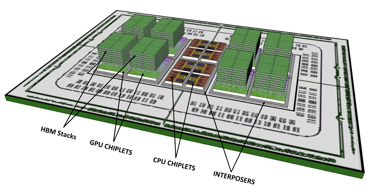](https://mlsysbook.ai/contents/core/hw_acceleration/images/png/chiplets.png "Figure 9: Chiplet Interconnect: Modern AI accelerators partition large designs into smaller chiplets and connect them via high-bandwidth interconnects, enabling scalability beyond monolithic die limitations and improving manufacturing yields. HBM stacks provide fast access to data, crucial for the memory-intensive workloads common in machine learning.")
Figure 9: **Chiplet Interconnect**: Modern AI accelerators partition large designs into smaller chiplets and connect them via high-bandwidth interconnects, enabling scalability beyond monolithic die limitations and improving manufacturing yields. HBM stacks provide fast access to data, crucial for the memory-intensive workloads common in machine learning.
Modern AI accelerators, such as AMD’s Instinct MI300, take this approach by integrating multiple compute chiplets alongside memory chiplets, linked by high-speed die-to-die interconnects. This modular design allows manufacturers to bypass the manufacturing limits of monolithic chips while still achieving high-density compute.
However, even within a single package, scaling is not without challenges. Inter-chiplet communication latency, memory coherence[32](https://mlsysbook.ai/contents/core/hw_acceleration/hw_acceleration.html#fn32)
, and thermal management become critical factors as more chiplets are integrated. Unlike traditional multi-chip systems, chiplet-based designs must carefully balance latency-sensitive workloads across multiple dies without introducing excessive bottlenecks.
32 **Memory Coherence**: Ensuring all processors in a system see the same consistent view of shared memory when multiple cores/chips access the same data. Traditional cache coherence protocols like MESI add 10-50 ns latency for multi-core CPUs. For AI accelerators with thousands of cores, coherence becomes prohibitively expensive—most ML hardware instead uses explicit memory management where programmers control data placement and synchronization manually.
### Multi-GPU Systems
Beyond chiplet-based designs, AI workloads often require multiple discrete GPUs working together. In multi-GPU systems, each accelerator has its own dedicated memory and compute resources, but they must efficiently share data and synchronize execution.
A common example is NVIDIA DGX systems, which integrate multiple GPUs connected via NVLink or PCIe. This architecture enables workloads to be split across GPUs, typically using data parallelism (where each GPU processes a different batch of data) or model parallelism (where different GPUs handle different parts of a neural network) ([Ben-Nun and Hoefler 2019](https://mlsysbook.ai/contents/core/hw_acceleration/hw_acceleration.html#ref-Ben-Nun2019data)
). These parallelization strategies are explored in depth in **[Chapter 8: AI Training](https://mlsysbook.ai/contents/core/training/training.html#sec-ai-training)
**.
Ben-Nun, Tal, and Torsten Hoefler. 2019. “Demystifying Parallel and Distributed Deep Learning: An in-Depth Concurrency Analysis.” _ACM Computing Surveys_ 52 (4): 1–43. [https://doi.org/10.1145/3320060](https://doi.org/10.1145/3320060)
.
As illustrated in [Figure 10](https://mlsysbook.ai/contents/core/hw_acceleration/hw_acceleration.html#fig-multi-gpu)
, NVSwitch interconnects enable high-speed communication between GPUs, reducing bottlenecks in distributed training. However, scaling up the number of GPUs introduces fundamental distributed coordination challenges that become the dominant performance constraint. The arithmetic intensity of transformer training (0.5-2 FLOPS/byte) forces frequent gradient synchronization across GPUs, where AllReduce operations must aggregate 175 billion parameters in GPT-3 scale models. NVSwitch provides 600 GB/s bidirectional bandwidth, but even this substantial interconnect becomes bandwidth-bound when 8 H100 GPUs simultaneously exchange gradients, creating a 4.8 TB/s aggregate demand that exceeds available capacity. The coordination complexity compounds exponentially—while two GPUs require a single communication channel, eight GPUs need 28 interconnect paths, and fault tolerance requirements mandate redundant communication patterns. Memory consistency protocols further complicate coordination as different GPUs may observe weight updates at different times, requiring sophisticated synchronization primitives that can add 10-50μs latency per training step—seemingly small delays that aggregate to hours of training time across million-iteration runs.
[](https://mlsysbook.ai/contents/core/hw_acceleration/98ab56e9be393ccdfd3a8bbee67360ac9fd51a2e.svg "Figure 10: Multi-GPU Scaling: NVSwitch interconnects enable high-bandwidth, low-latency communication between GPUs, overcoming PCIe bottlenecks for distributed training of large models. Scaling GPU count introduces challenges in maintaining memory consistency and efficiently scheduling workloads across interconnected devices.")
Figure 10: **Multi-GPU Scaling**: NVSwitch interconnects enable high-bandwidth, low-latency communication between GPUs, overcoming PCIe bottlenecks for distributed training of large models. Scaling GPU count introduces challenges in maintaining memory consistency and efficiently scheduling workloads across interconnected devices.
#### Communication Overhead and Amdahl’s Law Analysis
The fundamental limitation of distributed AI training stems from Amdahl’s Law, which quantifies how communication overhead constrains parallel speedup regardless of available compute power. For distributed neural network training, communication overhead during gradient synchronization creates a sequential bottleneck that limits scalability even with infinite parallelism.
The maximum speedup achievable with distributed training is bound by Amdahl’s Law: \\\[ \\text{Speedup} = \\frac{1}{(1-P) + \\frac{P}{N}} \\\] where \\(P\\) is the fraction of work that can be parallelized and \\(N\\) is the number of processors. However, for AI training, communication overhead introduces additional sequential time: \\\[ \\text{Speedup}\_{\\text{AI}} = \\frac{1}{(1-P) + \\frac{P}{N} + \\frac{C}{N}} \\\] where \\(C\\) represents the communication overhead fraction.
Consider training a 175 B parameter model with 1000 H100 GPUs as a concrete example:
* **Computation time per iteration**: 100 ms of forward/backward passes
* **Communication time**: AllReduce of 175 B parameters (700 GB in FP32) across 1000 GPUs
* **Available bandwidth**: 600 GB/s per NVSwitch link
* **Communication overhead**: \\(\\frac{700\\text{GB}}{600\\text{GB/s}} \\times \\log\_2(1000) \\approx 11.6\\text{ms}\\)
Even if only 5% of training requires communication (P = 0.95), the maximum speedup is: \\\[ \\text{Speedup} = \\frac{1}{0.05 + \\frac{0.95}{1000} + \\frac{0.116}{100}} \\approx 8.3\\text{x} \\\]
This demonstrates why adding more GPUs beyond ~100 provides diminishing returns for large model training.
Communication requirements scale superlinearly with model size and linearly with the number of parameters. Modern transformer models require gradient synchronization across all parameters during each training step:
* **GPT-3 (175 B parameters)**: 700 GB gradient exchange per step
* **GPT-4 (estimated 1.8 T parameters)**: ~7 TB gradient exchange per step
* **Future 10 T parameter models**: ~40 TB gradient exchange per step
Even with advanced interconnects like NVLink 4.0 (1.8 TB/s), gradient synchronization for 10 T parameter models would require 22+ seconds per training step, making distributed training impractical without algorithmic innovations like gradient compression or asynchronous updates.
Multi-GPU systems face additional bottlenecks from memory bandwidth competition. When 8 H100 GPUs simultaneously access HBM during gradient computation, the effective memory bandwidth per GPU drops from 3.35 TB/s to approximately 2.1 TB/s due to memory controller contention and NUMA effects. This 37% reduction in memory performance compounds communication overhead, further limiting scalability.
Understanding Amdahl’s Law guides optimization strategies:
1. **Gradient Compression**: Reduce communication volume by 10-100\\(\\times\\) through sparsification and quantization
2. **Pipeline Parallelism**: Overlap communication with computation to hide gradient synchronization latency
3. **Model Parallelism**: Partition models across devices to reduce gradient synchronization requirements
4. **Asynchronous Updates**: Relax consistency requirements to eliminate synchronization barriers
These techniques modify the effective value of \\(P\\) and \\(C\\) in Amdahl’s equation, enabling better scaling behavior at the cost of algorithmic complexity.
### TPU Pods
As models and datasets continue to expand, training and inference workloads must extend beyond single-server configurations. This scaling requirement has led to the development of sophisticated distributed systems where multiple accelerators communicate across networks. Google’s TPU Pods represent a pioneering approach to this challenge, interconnecting hundreds of TPUs to function as a unified system ([Norman P. Jouppi et al. 2020](https://mlsysbook.ai/contents/core/hw_acceleration/hw_acceleration.html#ref-Jouppi2020tpuv4)
).
Jouppi, Norman P., Doe Hyun Yoon, George Kurian, Sheng Li, Nishant Patil, James Laudon, Cliff Young, and David Patterson. 2020. “A Domain-Specific Supercomputer for Training Deep Neural Networks.” _Communications of the ACM_ 63 (7): 67–78. [https://doi.org/10.1145/3360307](https://doi.org/10.1145/3360307)
.
The architectural design of TPU Pods differs fundamentally from traditional multi-GPU systems. While multi-GPU configurations typically rely on NVLink or PCIe connections within a single machine, TPU Pods employ high-bandwidth optical links to interconnect accelerators at data center scale. This design implements a 2D torus interconnect topology, enabling efficient data exchange between accelerators while minimizing communication bottlenecks as workloads scale across nodes.
The effectiveness of this architecture is demonstrated in its performance scaling capabilities. As illustrated in [Figure 11](https://mlsysbook.ai/contents/core/hw_acceleration/hw_acceleration.html#fig-tpu-pod-perf)
, TPU Pod performance exhibits near-linear scaling when running ResNet-50, from quarter-pod to full-pod configurations. The system achieves a remarkable 33.0\\(\\times\\) speedup when scaled to 1024 chips compared to a 16-TPU baseline. This scaling efficiency is particularly noteworthy in larger configurations, where performance continues to scale strongly even as the system expands from 128 to 1024 chips.
[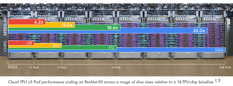](https://mlsysbook.ai/contents/core/hw_acceleration/images/png/tpu-pod-perf.png "Figure 11: Scaling Efficiency of TPU Pods: Increasing the number of TPU chips within a pod maintains near-linear performance gains on ResNet-50, achieving a 33.0\times speedup from 16 to 1024 chips. This efficient scaling provides the effectiveness of the 2D torus interconnect and high-bandwidth optical links in minimizing communication bottlenecks as workloads expand across multiple accelerators.")
Figure 11: **Scaling Efficiency of TPU Pods**: Increasing the number of TPU chips within a pod maintains near-linear performance gains on ResNet-50, achieving a 33.0\\(\\times\\) speedup from 16 to 1024 chips. This efficient scaling provides the effectiveness of the 2D torus interconnect and high-bandwidth optical links in minimizing communication bottlenecks as workloads expand across multiple accelerators.
However, distributing AI workloads across an entire data center introduces distributed coordination challenges that fundamentally differ from single-node systems. The 2D torus interconnect, while providing high bisection bandwidth, creates communication bottlenecks when training large transformer models that require AllReduce operations across all 1,024 TPUs. Each parameter gradient must traverse multiple hops through the torus network, with worst-case communication requiring 32 hops between distant TPUs, creating latency penalties that compound with model size.
The distributed memory architecture exacerbates coordination complexity—unlike multi-GPU systems with shared host memory, each TPU node maintains independent memory spaces, forcing explicit data marshaling and synchronization protocols. Network partition tolerance becomes critical as optical link failures can split the pod into disconnected islands, requiring sophisticated consensus algorithms to maintain training consistency.
The energy cost of coordination also scales dramatically: moving data across the pod’s optical interconnect consumes 1000\\(\\times\\) more energy than on-chip communication within individual TPUs, transforming distributed training into a careful balance between computation parallelism and communication efficiency where AllReduce bandwidth, not compute capacity, determines overall training throughput.
### Wafer-Scale AI
At the frontier of AI scaling, wafer-scale[33](https://mlsysbook.ai/contents/core/hw_acceleration/hw_acceleration.html#fn33)
integration represents a paradigm shift—abandoning traditional multi-chip architectures in favor of a single, massive AI processor. Rather than partitioning computation across discrete chips, this approach treats an entire silicon wafer as a unified compute fabric, eliminating the inefficiencies of inter-chip communication.
33 **Wafer-Scale Integration**: Using an entire 300 mm silicon wafer as a single processor instead of cutting it into individual chips. Cerebras WSE-3 contains 4 trillion transistors across 850,000 cores—125\\(\\times\\) more than the largest GPUs. Manufacturing challenges include 100% yield requirements (solved with redundant cores) and cooling 23 kW of power. This approach eliminates inter-chip communication delays but costs $2-3 million per wafer versus $40,000 for equivalent GPU clusters.
Systems, Cerebras. 2021a. “The Wafer-Scale Engine 2: Scaling AI Compute Beyond GPUs.” _Cerebras White Paper_. [https://cerebras.ai/product-chip/](https://cerebras.ai/product-chip/)
.
As shown in [Figure 12](https://mlsysbook.ai/contents/core/hw_acceleration/hw_acceleration.html#fig-processor-trends)
, Cerebras’ Wafer-Scale Engine (WSE) processors break away from the historical transistor scaling trends of CPUs, GPUs, and TPUs. While these architectures have steadily increased transistor counts along an exponential trajectory, WSE introduces an entirely new scaling paradigm, integrating trillions of transistors onto a single wafer—far surpassing even the most advanced GPUs and TPUs. With WSE-3, this trajectory continues, pushing wafer-scale AI to unprecedented levels ([Systems 2021a](https://mlsysbook.ai/contents/core/hw_acceleration/hw_acceleration.html#ref-Cerebras2021wse2)
).
[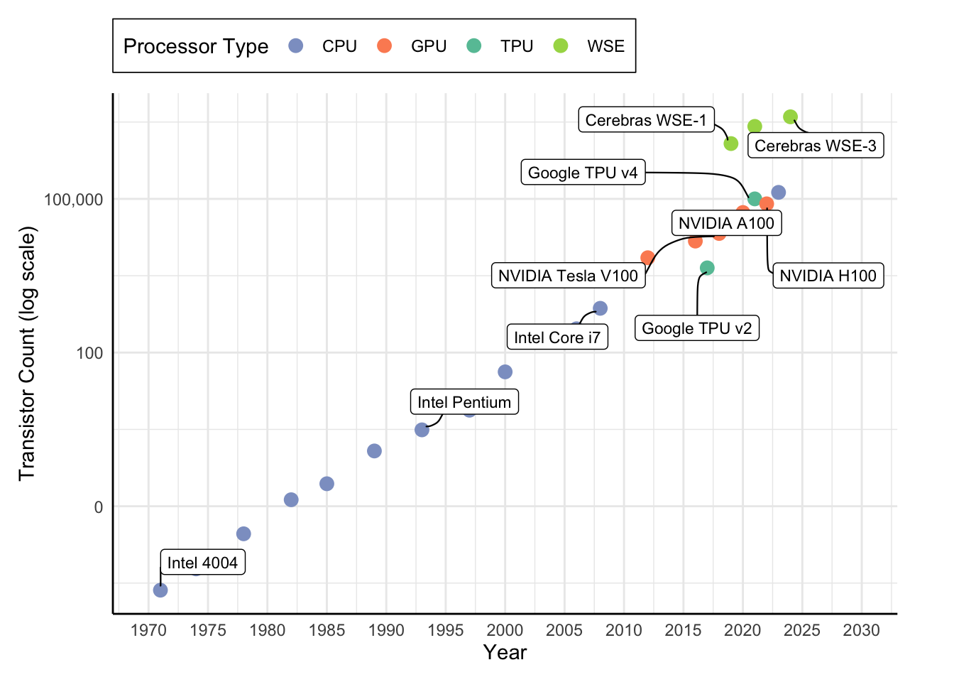](https://mlsysbook.ai/contents/core/hw_acceleration/hw_acceleration_files/figure-html/fig-processor-trends-1.png "Figure 12: Wafer-Scale Integration: Wafer-scale AI processors integrate trillions of transistors onto a single wafer, offering ultra-fast on-die communication to surpass traditional multi-chip architectures and achieve unprecedented performance levels.")
Figure 12: **Wafer-Scale Integration**: Wafer-scale AI processors integrate trillions of transistors onto a single wafer, offering ultra-fast on-die communication to surpass traditional multi-chip architectures and achieve unprecedented performance levels.
The fundamental advantage of wafer-scale AI is its ultra-fast, on-die communication. Unlike chiplets, GPUs, or TPU Pods, where data must traverse physical boundaries between separate devices, wafer-scale AI enables near-instantaneous data transfer across its vast compute array. This architecture drastically reduces communication latency, unlocking performance levels that are unachievable with conventional multi-chip systems.
However, achieving this level of integration introduces formidable engineering challenges. Thermal dissipation, fault tolerance, and manufacturing yield become major constraints when fabricating a processor of this scale. These sustainability challenges, including energy consumption and resource utilization, are examined in **[Chapter 18: Sustainable AI](https://mlsysbook.ai/contents/core/sustainable_ai/sustainable_ai.html#sec-sustainable-ai)
**. Unlike distributed TPU systems, which mitigate failures by dynamically re-routing workloads, wafer-scale AI must incorporate built-in redundancy mechanisms to tolerate localized defects in the silicon. Successfully addressing these challenges is essential to realizing the full potential of wafer-scale computing as the next frontier in AI acceleration.
### AI Systems Scaling Trajectory
[Table 20](https://mlsysbook.ai/contents/core/hw_acceleration/hw_acceleration.html#tbl-scaling-trajectory)
illustrates the progressive scaling of AI acceleration, from single-chip processors to increasingly complex architectures such as chiplet-based designs, multi-GPU systems, TPU Pods, and wafer-scale AI. Each step in this evolution introduces new challenges related to data movement, memory access, interconnect efficiency, and workload distribution. While chiplets enable modular scaling within a package, they introduce latency and memory coherence issues. Multi-GPU systems rely on high-speed interconnects like NVLink but face synchronization and communication bottlenecks. TPU Pods push scalability further by distributing workloads across clusters, yet they must contend with interconnect congestion and workload partitioning. At the extreme end, wafer-scale AI integrates an entire wafer into a single computational unit, presenting unique challenges in thermal management and fault tolerance.
Table 20: **AI Acceleration Trends**: Scaling AI systems provides increasing challenges in data movement and memory access, driving architectural innovations from chiplets to wafer-scale integration. Each approach introduces unique trade-offs between modularity, latency, and complexity, demanding careful consideration of interconnect efficiency and workload distribution.
| | | |
| --- | --- | --- |
| **Chiplets** | Modular scaling within a package | Inter-chiplet latency, memory coherence |
| **Multi-GPU** | External GPU interconnects (NVLink) | Synchronization overhead, communication bottlenecks |
| **TPU Pods** | Distributed accelerator clusters | Interconnect congestion, workload partitioning |
| **Wafer-Scale AI** | Entire wafer as a single processor | Thermal dissipation, fault tolerance |
### Computation and Memory Scaling Changes
As AI systems scale from single-chip accelerators to multi-chip architectures, the fundamental challenges in computation and memory evolve. In a single accelerator, execution is primarily optimized for locality—ensuring that computations are mapped efficiently to available processing elements while minimizing memory access latency. However, as AI systems extend beyond a single chip, the scope of these optimizations expands significantly. Computation must now be distributed across multiple accelerators, and memory access patterns become constrained by interconnect bandwidth and communication overhead.
#### Multi-chip Execution Mapping
In single-chip AI accelerators, computation placement is concerned with mapping workloads to PEs, vector units, and tensor cores. Mapping strategies aim to maximize data locality, ensuring that computations access nearby memory to reduce costly data movement.
As AI systems scale to multi-chip execution, computation placement must consider several critical factors. Workloads need to be partitioned across multiple accelerators, which requires explicit coordination of execution order and dependencies. This division is essential due to the inherent latency associated with cross-chip communication, which contrasts sharply with single-chip systems that benefit from shared on-chip memory. Accordingly, computation scheduling must be interconnect-aware to manage these delays effectively. Additionally, achieving load balancing across accelerators is vital; an uneven distribution of tasks can result in some accelerators remaining underutilized while others operate at full capacity, ultimately hindering overall system performance.
For example, in multi-GPU training, computation mapping must ensure that each GPU has a balanced portion of the workload while minimizing expensive cross-GPU communication. Similarly, in TPU Pods, mapping strategies must align with the torus interconnect topology, ensuring that computation is placed to minimize long-distance data transfers.
Thus, while computation placement in single-chip systems is a local optimization problem, in multi-chip architectures, it becomes a global optimization challenge where execution efficiency depends on minimizing inter-chip communication and balancing workload distribution.
#### Distributed Access Memory Allocation
Memory allocation strategies in single-chip AI accelerators are designed to minimize off-chip memory accesses by using on-chip caches, SRAM, and HBM. Techniques such as tiling, data reuse, and kernel fusion ensure that computations make efficient use of fast local memory.
In multi-chip AI systems, each accelerator manages its own local memory, which necessitates the explicit allocation of model parameters, activations, and intermediate data across the devices. Unlike single-chip execution where data is fetched once and reused, multi-chip setups require deliberate strategies to minimize redundant data transfers, as data must be communicated between accelerators. Additionally, when overlapping data is processed by multiple accelerators, the synchronization of shared data can introduce significant overhead that must be carefully managed to ensure efficient execution.
For instance, in multi-GPU deep learning, gradient synchronization across GPUs is a memory-intensive operation that must be optimized to avoid network congestion ([Shallue et al. 2019](https://mlsysbook.ai/contents/core/hw_acceleration/hw_acceleration.html#ref-Shallue2019measuring)
). In wafer-scale AI, memory allocation must account for fault tolerance and redundancy mechanisms, ensuring that defective regions of the wafer do not disrupt execution.
Shallue, Christopher J, Jaehoon Lee, Joseph Antognini, Jascha Sohl-Dickstein, Roy Frostig, and George E Dahl. 2019. “Measuring the Effects of Data Parallelism on Neural Network Training.” _Journal of Machine Learning Research_ 20: 1–49. [http://jmlr.org/papers/v20/18-789.html](http://jmlr.org/papers/v20/18-789.html)
.
Thus, while memory allocation in single-chip accelerators focuses on local cache efficiency, in multi-chip architectures, it must be explicitly coordinated across accelerators to balance memory bandwidth, minimize redundant transfers, and reduce synchronization overhead.
#### Data Movement Constraints
In single-chip AI accelerators, data movement optimization is largely focused on minimizing on-chip memory access latency. Techniques such as weight stationarity, input stationarity, and tiling ensure that frequently used data remains close to the execution units, reducing off-chip memory traffic.
In multi-chip architectures, data movement transcends being merely an intra-chip issue and becomes a significant system-wide bottleneck. Scaling introduces several critical challenges, foremost among them being inter-chip bandwidth constraints; communication links such as PCIe, NVLink, and TPU interconnects operate at speeds that are considerably slower than those of on-chip memory accesses. Additionally, when accelerators share model parameters or intermediate computations, the resulting data synchronization overhead, which encompass latency and contention, can markedly impede execution. Finally, optimizing collective communication is essential for workloads that require frequent data exchanges, such as gradient updates in deep learning training, where minimizing synchronization penalties is imperative for achieving efficient system performance.
For example, in TPU Pods, systolic execution models ensure that data moves in structured patterns, reducing unnecessary off-chip transfers. In multi-GPU inference, techniques like asynchronous data fetching and overlapping computation with communication help mitigate inter-chip latency.
Thus, while data movement optimization in single-chip systems focuses on cache locality and tiling, in multi-chip architectures, the primary challenge is reducing inter-chip communication overhead to maximize efficiency.
#### Compilers and Runtimes Adaptation
As AI acceleration extends beyond a single chip, compilers and runtimes must adapt to manage computation placement, memory organization, and execution scheduling across multiple accelerators. The fundamental principles of locality, parallelism, and efficient scheduling remain essential, but their implementation requires new strategies for distributed execution.
One of the primary challenges in scaling AI execution is computation placement. In a single-chip accelerator, workloads are mapped to processing elements, vector units, and tensor cores with an emphasis on minimizing on-chip data movement and maximizing parallel execution. However, in a multi-chip system, computation must be partitioned hierarchically, where workloads are distributed not just across cores within a chip, but also across multiple accelerators. Compilers handle this by implementing interconnect-aware scheduling, optimizing workload placement to minimize costly inter-chip communication.
Similarly, memory management evolves as scaling extends beyond a single accelerator. In a single-chip system, local caching, HBM reuse, and efficient tiling strategies ensure that frequently accessed data remains close to computation units. However, in a multi-chip system, each accelerator has its own independent memory, requiring explicit memory partitioning and coordination. Compilers optimize memory layouts for distributed execution, while runtimes introduce data prefetching and caching mechanisms to reduce inter-chip memory access overhead.
Beyond computation and memory, data movement becomes a major bottleneck at scale. In a single-chip accelerator, efficient on-chip caching and minimized DRAM accesses ensure that data is reused efficiently. However, in a multi-chip system, communication-aware execution becomes critical, requiring compilers to generate execution plans that overlap computation with data transfers. Runtimes handle inter-chip synchronization, ensuring that workloads are not stalled by waiting for data to arrive from remote accelerators.
Finally, execution scheduling must be extended for global coordination. In single-chip AI execution, scheduling is primarily concerned with parallelism and maximizing compute occupancy within the accelerator. However, in a multi-chip system, scheduling must balance workload distribution across accelerators while taking interconnect bandwidth and synchronization latency into account. Runtimes manage this complexity by implementing adaptive scheduling strategies that dynamically adjust execution plans based on system state and network congestion.
[Table 21](https://mlsysbook.ai/contents/core/hw_acceleration/hw_acceleration.html#tbl-scaling-adaptations)
summarizes these key adaptations, highlighting how compilers and runtimes extend their capabilities to efficiently support multi-chip AI execution.
Thus, while the fundamentals of AI acceleration remain intact, compilers and runtimes must extend their functionality to operate efficiently across distributed systems. The next section will explore how mapping strategies evolve to further optimize multi-chip AI execution.
Table 21: **Multi-Chip Adaptations**: Efficient AI execution on multiple accelerators requires coordinated adjustments to computation placement, memory management, and scheduling to balance workload distribution and minimize communication overhead. Compilers and runtimes extend their capabilities to dynamically adapt to system state and network congestion, enabling scalable and performant multi-chip AI systems.
| | | |
| --- | --- | --- |
| **Computation Placement** | Local PEs, tensor cores, vector units | Hierarchical mapping, interconnect-aware scheduling |
| **Memory Management** | Caching, HBM reuse, local tiling | Distributed allocation, prefetching, caching |
| **Data Movement** | On-chip reuse, minimal DRAM access | Communication-aware execution, overlap transfers |
| **Execution Scheduling** | Parallelism, compute occupancy | Global scheduling, interconnect-aware balancing |
### Execution Models Adaptation
As AI accelerators scale beyond a single chip, execution models must evolve to account for the complexities introduced by distributed computation, memory partitioning, and inter-chip communication. In single-chip accelerators, execution is optimized for local processing elements, with scheduling strategies that balance parallelism, locality, and data reuse. However, in multi-chip AI systems, execution must now be coordinated across multiple accelerators, introducing new challenges in workload scheduling, memory coherence, and interconnect-aware execution.
This section explores how execution models change as AI acceleration scales, focusing on scheduling, memory coordination, and runtime management in multi-chip systems.
#### Cross-Accelerator Scheduling
In single-chip AI accelerators, execution scheduling is primarily aimed at optimizing parallelism within the processor. This involves ensuring that workloads are effectively mapped to tensor cores, vector units, and special function units by employing techniques designed to enhance data locality and resource utilization. For instance, static scheduling uses a predetermined execution order that is carefully optimized for locality and reuse, while dynamic scheduling adapts in real time to variations in workload demands. Additionally, pipeline execution divides computations into stages, thereby maximizing hardware utilization by maintaining a continuous flow of operations.
In contrast, scheduling in multi-chip architectures must address the additional challenges posed by inter-chip dependencies. Workload partitioning in such systems involves distributing tasks across various accelerators such that each receives an optimal share of the workload, all while minimizing the overhead caused by excessive communication. Interconnect-aware scheduling is essential to align execution timing with the constraints of inter-chip bandwidth, thus preventing performance stalls. Latency hiding techniques also play a critical role, as they enable the overlapping of computation with communication, effectively reducing waiting times.
For example, in multi-GPU inference scenarios, execution scheduling is implemented in a way that allows data to be prefetched concurrently with computation, thereby mitigating memory stalls. Similarly, TPU Pods leverage the systolic array model to tightly couple execution scheduling with data flow, ensuring that each TPU core receives its required data precisely when needed. Therefore, while single-chip execution scheduling is focused largely on maximizing internal parallelism, multi-chip systems require a more holistic approach that explicitly manages communication overhead and synchronizes workload distribution across accelerators.
#### Cross-Accelerator Coordination
In single-chip AI accelerators, memory coordination is managed through sophisticated local caching strategies that keep frequently used data in close proximity to the execution units. Techniques such as tiling, kernel fusion, and data reuse are employed to reduce the dependency on slower memory hierarchies, thereby enhancing performance and reducing latency.
In contrast, multi-chip architectures present a distributed memory coordination challenge that necessitates more deliberate management. Each accelerator in such a system possesses its own independent memory, which must be organized through explicit memory partitioning to minimize cross-chip data accesses. Additionally, ensuring consistency and synchronization of shared data across accelerators is essential to maintain computational correctness. Efficient communication mechanisms must also be implemented to schedule data transfers in a way that limits overhead associated with synchronization delays.
For instance, in distributed deep learning training, model parameters must be synchronized across multiple GPUs using methods such as all-reduce, where gradients are aggregated across accelerators while reducing communication latency. In wafer-scale AI, memory coordination must further address fault-tolerant execution, ensuring that defective areas do not compromise overall system performance. Consequently, while memory coordination in single-chip systems is primarily concerned with cache optimization, multi-chip architectures require management of distributed memory access, synchronization, and communication to achieve efficient execution.
#### Cross-Accelerator Execution Management
Execution in single-chip AI accelerators is managed by AI runtimes that handle workload scheduling, memory allocation, and hardware execution. These runtimes optimize execution at the kernel level, ensuring that computations are executed efficiently within the available resources.
In multi-chip AI systems, runtimes must incorporate a strategy for distributed execution orchestration. This approach ensures that both computation and memory access are seamlessly coordinated across multiple accelerators, enabling efficient utilization of hardware resources and minimizing bottlenecks associated with data transfers.
These systems require robust mechanisms for cross-chip workload synchronization. Careful management of dependencies and timely coordination between accelerators are essential to prevent stalls in execution that may arise from delays in inter-chip communication. Such synchronization is critical for maintaining the flow of computation, particularly in environments where latency can significantly impact overall performance.
Finally, adaptive execution models play a pivotal role in contemporary multi-chip architectures. These models dynamically adjust execution plans based on current hardware availability and communication constraints, ensuring that the system can respond to changing conditions and optimize performance in real time. Together, these strategies provide a resilient framework for managing the complexities of distributed AI execution.
For example, in Google’s TPU Pods, the TPU runtime is responsible for scheduling computations across multiple TPU cores, ensuring that workloads are executed in a way that minimizes communication bottlenecks. In multi-GPU frameworks like PyTorch and TensorFlow, runtime execution must synchronize operations across GPUs, ensuring that data is transferred efficiently while maintaining execution order.
Thus, while single-chip runtimes focus on optimizing execution within a single processor, multi-chip runtimes must handle system-wide execution, balancing computation, memory, and interconnect performance.
#### Computation Placement Adaptation
As AI systems expand beyond single-chip execution, computation placement must adapt to account for inter-chip workload distribution and interconnect efficiency. In single-chip accelerators, compilers optimize placement by mapping workloads to tensor cores, vector units, and PEs, ensuring maximum parallelism while minimizing on-chip data movement. However, in multi-chip systems, placement strategies must address interconnect bandwidth constraints, synchronization latency, and hierarchical workload partitioning across multiple accelerators.
[Table 22](https://mlsysbook.ai/contents/core/hw_acceleration/hw_acceleration.html#tbl-computation-placement)
highlights these adaptations. To reduce expensive cross-chip communication, compilers now implement interconnect-aware workload partitioning, strategically assigning computations to accelerators based on communication cost. For instance, in multi-GPU training, compilers optimize placement to minimize NVLink or PCIe traffic, whereas TPU Pods leverage the torus interconnect topology to enhance data exchanges.
Table 22: **Computation Placement Strategies**: Multi-chip AI systems necessitate hierarchical workload mapping to minimize communication overhead; compilers adapt single-chip optimization techniques by considering interconnect bandwidth and latency when assigning computations to accelerators. This table contrasts computation placement in single-chip systems—local to processing elements—with multi-chip systems, where placement strategies prioritize efficient data exchange across accelerators.
| | | |
| --- | --- | --- |
| **Computation Placement** | Local PEs, tensor cores, vector units | Hierarchical mapping, interconnect-aware scheduling |
| **Workload Distribution** | Optimized within a single chip | Partitioning across accelerators, minimizing inter-chip communication |
| **Synchronization** | Managed within local execution units | Runtimes dynamically balance workloads, adjust execution plans |
Runtimes complement this by dynamically managing execution workloads, adjusting placement in real-time to balance loads across accelerators. Unlike static compilation, which assumes a fixed hardware topology, AI runtimes continuously monitor system conditions and migrate tasks as needed to prevent bottlenecks. This ensures efficient execution even in environments with fluctuating workload demands or varying hardware availability.
Thus, computation placement at scale builds upon local execution optimizations while introducing new challenges in inter-chip coordination, communication-aware execution, and dynamic load balancing—challenges that extend to how memory hierarchies must adapt to support efficient execution across multi-chip architectures.
### Navigating Multi-Chip AI Complexities
The evolution of AI hardware, from single-chip accelerators to multi-chip systems and wafer-scale integration, highlights the increasing complexity of efficiently executing large-scale machine learning workloads. Scaling AI systems introduces new challenges in computation placement, memory management, and data movement. While the fundamental principles of AI acceleration remain consistent, their implementation must adapt to the constraints of distributed execution, interconnect bandwidth limitations, and synchronization overhead.
Multi-chip AI architectures represent a significant step forward in addressing the computational demands of modern machine learning models. By distributing workloads across multiple accelerators, these systems offer increased performance, memory capacity, and scalability. However, realizing these benefits requires careful consideration of how computations are mapped to hardware, how memory is partitioned and accessed, and how execution is scheduled across a distributed system.
While we an overview of the key concepts and challenges in multi-chip AI acceleration as they extend beyond a single system, there is still much more to explore. As AI models continue to grow in size and complexity, new architectural innovations, mapping strategies, and runtime optimizations will be needed to sustain efficient execution. These emerging trends and future directions continue to evolve rapidly in the field. The ongoing development of AI hardware and software reflects a broader trend in computing, where specialization and domain-specific architectures are becoming increasingly important for addressing the unique demands of emerging workloads.
Understanding the principles and trade-offs involved in multi-chip AI acceleration enables machine learning engineers and system designers to make informed decisions about how to best deploy and optimize their models. Whether training large language models on TPU pods or deploying computer vision applications on multi-GPU systems, the ability to efficiently map computations to hardware will continue to be a critical factor in realizing the full potential of AI.
**Self-Check: Question 1.9**
1. What is a primary challenge when transitioning from single-chip to multi-chip AI architectures?
1. Maximizing utilization within fixed resources
2. Increasing the clock speed of individual chips
3. Reducing the size of individual processors
4. Balancing computational distribution against communication overhead
2. Explain how memory coherence challenges differ between chiplet-based architectures and traditional multi-chip systems.
3. True or False: In multi-GPU systems, increasing the number of GPUs always leads to linear performance gains.
4. The fundamental limitation of distributed AI training is that communication overhead constrains parallel speedup according to established \_\_\_\_\_ principles.
5. In a multi-accelerator system design, what is a critical factor that affects performance scaling?
1. The number of CPUs in the system
2. The efficiency of the specialized interconnect architecture
3. The use of PCIe interconnects
4. The clock speed of individual accelerators
[See Answers →](https://mlsysbook.ai/contents/core/hw_acceleration/hw_acceleration.html#quiz-answer-sec-ai-acceleration-multichip-ai-acceleration-38d7)
Heterogeneous SoC AI Acceleration
---------------------------------
The multi-chip architectures examined in previous sections focused primarily on maximizing computational throughput for data center workloads, where power budgets extend to kilowatts and cooling infrastructure supports rack-scale deployments. However, the hardware acceleration principles established—specialized compute units, memory hierarchy optimization, and workload mapping strategies—must adapt dramatically when deploying AI systems in mobile and edge environments. A smartphone operates within a 2 to 5 watt power budget, autonomous vehicles require deterministic real-time guarantees, and IoT sensors must function for years on battery power. These constraints necessitate heterogeneous System-on-Chip (SoC) architectures that coordinate multiple specialized processors within a single chip while meeting stringent power, thermal, and latency requirements fundamentally different from data center deployments.
The mobile AI revolution has fundamentally transformed how we think about AI acceleration, moving beyond homogeneous data center architectures to heterogeneous System-on-Chip (SoC) designs that coordinate multiple specialized processors. Modern smartphones, automotive systems, and IoT devices integrate CPU cores, GPU shaders, digital signal processors (DSPs), and dedicated neural processing units (NPUs) within a single chip, requiring sophisticated orchestration to achieve optimal performance under strict power and thermal constraints.
### Mobile SoC Architecture Evolution
Qualcomm’s Snapdragon AI Engine exemplifies heterogeneous computing for mobile AI, coordinating Kryo CPU cores, Adreno GPU, Hexagon DSP, and dedicated NPU[34](https://mlsysbook.ai/contents/core/hw_acceleration/hw_acceleration.html#fn34)
across a shared memory hierarchy. The Snapdragon 8 Gen 3 achieves 73 TOPS through intelligent workload distribution—computer vision kernels execute on the GPU’s parallel shaders, audio processing leverages the DSP’s specialized arithmetic units, while transformer attention mechanisms utilize the NPU’s optimized matrix engines. This coordination requires millisecond-precision scheduling to meet real-time constraints while managing thermal throttling and battery life optimization.
34 **Neural Processing Unit (NPU)**: Specialized processors designed specifically for neural network inference, distinct from general-purpose GPUs. Apple introduced the first consumer NPU in the A11 chip (2017), achieving 600 billion operations per second while consuming less than 1 watt. Modern NPUs like Apple’s M3 Neural Engine deliver 18 TOPS for on-device AI tasks like real-time image processing, voice recognition, and computational photography. NPUs excel at low-power, fixed-function AI workloads but lack the programmability of GPUs for diverse ML research.
While Qualcomm’s approach emphasizes diverse processor specialization, Apple’s vertically integrated strategy demonstrates how tight hardware-software co-design enables even more sophisticated heterogeneous execution. The M2 chip’s 16-core Neural Engine (15.8 TOPS) coordinates with the 10-core GPU and 8-core CPU through a unified memory architecture that eliminates data copying overhead. The Neural Engine’s specialized matrix multiplication units handle transformer layers, while the GPU’s Metal Performance Shaders accelerate convolutional operations, and the CPU manages control flow and dynamic layer selection. This fine-grained coordination enables real-time language translation and on-device image generation while maintaining millisecond response times.
Beyond these vertically integrated solutions from Qualcomm and Apple, ARM’s IP licensing model offers a fundamentally different approach that enables SoC designers to customize processor combinations based on target applications. The Mali-G78 GPU’s 24 cores can be paired with Ethos-N78 NPU for balanced general-purpose and AI acceleration, while the Cortex-M55 microcontroller integrates Ethos-U55 microNPU for ultra-low-power edge applications. This modular flexibility allows automotive SoCs to emphasize deterministic real-time processing while smartphone SoCs optimize for interactive performance and battery efficiency.
### Strategies for Dynamic Workload Distribution
With multiple specialized processors available on heterogeneous SoCs, the critical challenge becomes intelligently distributing neural network operations across these resources to maximize performance while respecting power and latency constraints.
Modern neural networks require intelligent partitioning across heterogeneous processors based on operation characteristics and current system state. Convolutional layers with regular data access patterns typically execute efficiently on GPU shader cores, while fully connected layers with irregular sparsity patterns may perform better on general-purpose CPU cores with large caches. Attention mechanisms in transformers benefit from NPU matrix engines when sequences are long, but may execute more efficiently on CPU when sequence lengths are small due to the NPU setup overhead.
Beyond static operation-to-processor mapping, heterogeneous SoCs implement dynamic processor selection based on multiple constraints:
* **Power Budget**: During battery operation, the system may route computations to lower-power DSP cores rather than high-performance GPU cores
* **Thermal State**: When approaching thermal limits, workloads shift from power-hungry NPU to more efficient CPU execution
* **Latency Requirements**: Safety-critical automotive applications prioritize deterministic CPU execution over potentially faster but variable NPU processing
* **Concurrent Workload Interference**: Multiple AI applications may require load balancing across available processors to maintain Quality of Service
Compounding the processor selection challenge, shared memory architectures require sophisticated arbitration when multiple processors access LPDDR simultaneously. The Snapdragon 8 Gen 3’s memory controller implements priority-based scheduling where camera processing receives higher priority than background AI tasks, ensuring real-time video processing while background neural networks adapt their execution patterns to available memory bandwidth. This arbitration becomes critical during memory-intensive operations like large language model inference, where parameter streaming from DRAM must be carefully coordinated across processors.
### Power and Thermal Management
Mobile AI workloads must maintain high performance while operating within strict power budgets and thermal envelopes—constraints that require sophisticated coordination across heterogeneous processors.
Heterogeneous SoCs implement coordinated DVFS across multiple processors to optimize the power-performance envelope. When one processor increases frequency to meet latency demands, the system may reduce voltage on other processors to maintain total power budget. This coordination becomes complex in AI workloads where computational phases may shift rapidly between processors—the system must predict upcoming workload transitions to preemptively adjust operating points while avoiding voltage/frequency oscillations that degrade efficiency.
When DVFS alone cannot maintain the power envelope, mobile SoCs implement thermal throttling through intelligent task migration rather than simple frequency reduction. When the NPU approaches thermal limits during intensive neural network processing, the runtime system can migrate layers to the GPU or CPU while maintaining computational throughput. This approach preserves performance during thermal events, though it requires sophisticated workload characterization to predict execution time and power consumption across different processors.
Beyond real-time power and thermal management, mobile AI systems must also adapt their computational strategies based on battery state and charging status. During low battery conditions, the system may switch from high-accuracy models to efficient approximations, migrate workloads from power-hungry NPU to energy-efficient DSP, or reduce inference frequency while maintaining application responsiveness. Conversely, during charging, the system can enable higher-performance models and increase processing frequency to deliver enhanced user experiences.
### Automotive Heterogeneous AI Systems
Automotive applications introduce unique heterogeneous computing challenges that combine mobile-style power efficiency with hard real-time guarantees and functional safety requirements—a combination that demands fundamentally different architectural approaches.
Automotive SoCs must guarantee deterministic inference latency for safety-critical functions while supporting advanced driver assistance systems (ADAS). The Snapdragon Ride platform coordinates multiple AI accelerators across safety domains—redundant processing elements ensure functional safety compliance while high-performance accelerators handle perception, planning, and control algorithms. This architecture requires temporal isolation between safety-critical and convenience functions, implemented through hardware partitioning and time-triggered scheduling.
These safety requirements become even more complex when considering that modern vehicles integrate multiple AI-enabled SoCs for different domains—vision processing SoCs handle camera-based perception, radar processing SoCs manage RF sensor data, while central compute platforms coordinate high-level decision making. These distributed systems must maintain temporal coherence across sensor modalities with microsecond-precision timing, requiring specialized inter-SoC communication protocols and distributed synchronization mechanisms.
Extending beyond the vehicle’s internal sensors, vehicle-to-everything (V2X) communication adds another layer of heterogeneous processing where AI algorithms must coordinate local sensor processing with information received from other vehicles and infrastructure. This requires ultra-low latency processing chains where 5G modems, AI accelerators, and control systems operate within millisecond deadlines while maintaining functional safety requirements.
### Software Stack Challenges
The architectural sophistication of heterogeneous SoCs creates substantial software development challenges that span programming models, memory management, and runtime optimization.
Programming heterogeneous SoCs requires frameworks that abstract processor differences while exposing performance-critical optimization opportunities. OpenCL and Vulkan provide cross-processor execution, but achieving optimal performance requires processor-specific optimizations that complicate portable development. Modern ML frameworks like TensorFlow Lite and PyTorch Mobile implement automatic processor selection, but developers still need to understand heterogeneous execution patterns to achieve optimal results.
Complicating the programming challenge further, heterogeneous SoCs with shared memory architectures require sophisticated memory management that considers processor-specific caching behaviors, memory access patterns, and coherency requirements. CPU caches may interfere with GPU memory access patterns, while NPU direct memory access (DMA) operations must be synchronized with CPU cache operations to maintain data consistency.
To address the complexity of manual optimization across these dimensions, advanced heterogeneous SoCs implement machine learning-based runtime optimization that learns from execution patterns to improve processor selection, thermal management, and power optimization. These systems collect telemetry on workload characteristics, processor utilization, and power consumption to build models that predict optimal execution strategies for new workloads.
This heterogeneous approach to AI acceleration represents the future of computing, where no single processor architecture can optimally handle the diverse computational patterns in modern AI applications. Understanding these coordination challenges is essential for developing efficient mobile AI systems that deliver high performance while meeting the strict power, thermal, and real-time constraints of edge deployment scenarios.
However, the complexity of these heterogeneous systems creates numerous opportunities for misconception and suboptimal design decisions. The following fallacies and pitfalls highlight common misunderstandings that can undermine acceleration strategies.
**Self-Check: Question 1.10**
1. What is a primary reason for using heterogeneous SoC architectures in mobile AI systems?
1. To increase computational throughput without power constraints.
2. To maximize data center workload efficiency.
3. To simplify the design process by using a single type of processor.
4. To coordinate multiple specialized processors within strict power and thermal limits.
2. Explain how dynamic workload distribution strategies in heterogeneous SoCs help manage power and thermal constraints.
3. Order the following steps in managing workload distribution on a heterogeneous SoC: (1) Assess system power budget, (2) Evaluate processor thermal state, (3) Allocate tasks based on constraints, (4) Monitor performance and adjust.
4. Which of the following best describes a challenge in programming heterogeneous SoCs?
1. Managing memory coherency across diverse processors.
2. Ensuring all processors use the same programming model.
3. Achieving optimal performance without considering processor-specific optimizations.
4. Implementing a single execution strategy for all tasks.
5. In a production system, what trade-offs might you consider when implementing AI acceleration on a heterogeneous SoC for an autonomous vehicle?
[See Answers →](https://mlsysbook.ai/contents/core/hw_acceleration/hw_acceleration.html#quiz-answer-sec-ai-acceleration-heterogeneous-soc-ai-acceleration-b1bb)
Fallacies and Pitfalls
----------------------
Hardware acceleration involves complex interactions between specialized architectures, software stacks, and workload characteristics that create significant opportunities for misunderstanding optimal deployment strategies. The impressive performance numbers often associated with AI accelerators can mask important constraints and trade-offs that determine real-world effectiveness across different deployment scenarios.
**Fallacy:** _More specialized hardware always provides better performance than general-purpose alternatives._
This belief assumes that specialized accelerators automatically outperform general-purpose processors for all AI workloads. Specialized hardware achieves peak performance only when workloads match the architectural assumptions and optimization targets. Models with irregular memory access patterns, small batch sizes, or dynamic computation graphs may perform better on flexible general-purpose processors than on specialized accelerators designed for dense, regular computations. The overhead of data movement, format conversion, and synchronization can eliminate the benefits of specialized computation. Effective hardware selection requires matching workload characteristics to architectural strengths rather than assuming specialization always wins.
**Pitfall:** _Ignoring memory bandwidth limitations when selecting acceleration strategies._
Many practitioners focus on computational throughput metrics without considering memory bandwidth constraints that often limit real-world performance. AI accelerators with impressive computational capabilities can be severely bottlenecked by insufficient memory bandwidth, leading to poor hardware utilization. The ratio between computation intensity and memory access requirements determines whether an accelerator can achieve its theoretical performance. This oversight leads to expensive hardware deployments that fail to deliver expected performance improvements because the workload is memory-bound rather than compute-bound.
**Fallacy:** _Hardware acceleration benefits scale linearly with additional accelerators._
This misconception drives teams to expect proportional performance gains when adding more accelerators to their systems. Multi-accelerator setups introduce communication overhead, synchronization costs, and load balancing challenges that can severely limit scaling efficiency. Small models may not provide enough parallel work to utilize multiple accelerators effectively, while large models may be limited by communication bandwidth between devices. Distributed training and inference face additional challenges from gradient aggregation, model partitioning, and coordination overhead that create non-linear scaling relationships.
**Pitfall:** _Vendor-specific optimizations without considering long-term portability and flexibility._
Organizations often optimize exclusively for specific hardware vendors to achieve maximum performance without considering the implications for system flexibility and future migration. Deep integration with vendor-specific libraries, custom kernels, and proprietary optimization tools creates lock-in that complicates hardware upgrades, vendor changes, or multi-vendor deployments. While vendor-specific optimizations can provide significant performance benefits, they should be balanced against the need for system portability and the ability to adapt to evolving hardware landscapes. Maintaining some level of hardware abstraction preserves strategic flexibility while still capturing most performance benefits.
**Self-Check: Question 1.11**
1. Which of the following scenarios would most likely benefit from using general-purpose processors over specialized hardware accelerators?
1. A workload with irregular memory access patterns and dynamic computation graphs.
2. A workload with dense, regular computations and large batch sizes.
3. A workload that requires high computational throughput with minimal memory access.
4. A workload optimized for a specific vendor’s proprietary libraries.
2. True or False: Adding more accelerators to a system will always result in linear performance improvements.
3. Explain why memory bandwidth limitations can undermine the performance benefits of AI accelerators.
4. The belief that hardware acceleration benefits scale linearly with additional accelerators is a common \_\_\_\_. This misconception overlooks the communication and synchronization overheads that limit scaling efficiency.
5. In a production system, what trade-offs should be considered when optimizing for vendor-specific hardware?
[See Answers →](https://mlsysbook.ai/contents/core/hw_acceleration/hw_acceleration.html#quiz-answer-sec-ai-acceleration-fallacies-pitfalls-dc1f)
Summary
-------
Hardware acceleration has emerged as the critical enabler that transforms machine learning from academic curiosity to practical reality, fundamentally reshaping how we design both computational systems and the algorithms that run on them. The evolution from general-purpose processors to specialized AI accelerators represents more than just incremental improvement—it reflects a paradigm shift toward domain-specific computing where hardware and software are co-designed to optimize specific computational patterns. The journey from CPUs through GPUs to specialized TPUs, NPUs, and wafer-scale systems demonstrates how understanding workload characteristics drives architectural innovation, creating opportunities for orders-of-magnitude performance improvements through targeted specialization.
The technical challenges of AI acceleration span multiple layers of the computing stack, from low-level memory hierarchy optimization to high-level compiler transformations and runtime orchestration. Memory bandwidth limitations create fundamental bottlenecks that require sophisticated techniques like data tiling, kernel fusion, and hierarchy-aware scheduling to overcome. Mapping neural network computations to hardware involves complex trade-offs between different dataflow patterns, memory allocation strategies, and execution scheduling approaches that must balance computational efficiency with resource utilization.
Building on these foundational concepts, the emergence of multi-chip and distributed acceleration systems introduces additional complexities around communication overhead, memory coherence, and workload partitioning that require careful system-level optimization.
Key Takeaways
* Specialized AI accelerators achieve performance gains through domain-specific architectures optimized for tensor operations and dataflow patterns
* Memory hierarchy management is often the primary bottleneck in AI acceleration, requiring sophisticated data movement optimization strategies
* Hardware-software co-design enables order-of-magnitude improvements by aligning algorithm characteristics with architectural capabilities
* Multi-chip scaling introduces distributed computing challenges that require new approaches to communication, synchronization, and resource management
The principles of hardware acceleration established here provide the foundation for understanding how benchmarking methodologies evaluate accelerator performance and how deployment strategies must account for hardware constraints and capabilities. As AI models continue growing in complexity and computational requirements, the ability to effectively leverage specialized hardware becomes increasingly critical for practical system deployment, influencing everything from energy efficiency and cost optimization to the feasibility of real-time inference and large-scale training across diverse application domains.
**Self-Check: Question 1.12**
1. Which of the following best describes the primary advantage of hardware-software co-design in AI accelerators?
1. Reduced hardware costs
2. Simplified software development
3. Improved computational efficiency
4. Increased general-purpose applicability
2. Explain how memory hierarchy management can become a bottleneck in AI acceleration and how it can be mitigated.
3. Order the following steps in optimizing a multi-chip AI acceleration system: (1) Workload partitioning, (2) Communication overhead reduction, (3) Memory coherence management.
[See Answers →](https://mlsysbook.ai/contents/core/hw_acceleration/hw_acceleration.html#quiz-answer-sec-ai-acceleration-summary-a5f8)
Self-Check Answers
------------------
**Self-Check: Answer 1.1**
1. **What is the primary reason for the shift from general-purpose processors to domain-specific hardware in machine learning systems?**
1. To reduce the cost of hardware components
2. To improve the parallel processing capabilities and efficiency
3. To simplify the design of machine learning algorithms
4. To increase the utilization of existing software optimizations
_Answer_: The correct answer is B. To improve the parallel processing capabilities and efficiency. This shift is driven by the need to address the architectural misalignments of general-purpose processors with the parallel, data-intensive nature of ML workloads.
_Learning Objective_: Understand the motivations behind using domain-specific hardware in ML systems.
2. **True or False: Hardware acceleration in machine learning systems only focuses on improving computational speed, not energy efficiency.**
_Answer_: False. Hardware acceleration also aims to improve energy efficiency, as data movement energy costs typically exceed computational energy by more than two orders of magnitude.
_Learning Objective_: Recognize the dual goals of hardware acceleration: improving computational speed and energy efficiency.
3. **How do architectural selection decisions impact system-level performance in machine learning systems?**
_Answer_: Architectural selection decisions impact system-level performance by determining the efficiency of computations, energy usage, and implementation complexity. For example, choosing between GPUs, TPUs, or neuromorphic processors affects how well a system can handle specific ML workloads. This is important because it influences the overall effectiveness and cost-efficiency of deploying ML systems.
_Learning Objective_: Analyze the impact of different hardware architectures on ML system performance.
4. **Which of the following architectural innovations is used to optimize matrix multiplication in machine learning workloads?**
1. Floating-point coprocessors
2. Sequential processing models
3. Systolic array architectures
4. High-bandwidth memory interfaces
_Answer_: The correct answer is C. Systolic array architectures. These are used to optimize matrix multiplication by efficiently managing data flow and computation.
_Learning Objective_: Identify architectural innovations that optimize key ML operations.
5. **In a production system, what trade-offs might you consider when choosing between single-chip and multi-chip architectures for AI acceleration?**
_Answer_: When choosing between single-chip and multi-chip architectures, trade-offs include balancing computational parallelism with inter-chip communication overhead. Single-chip solutions may offer lower latency and simpler integration, while multi-chip architectures can provide greater computational capacity but may introduce complexity and communication delays. This is important because it affects the scalability and performance of AI systems in different deployment contexts.
_Learning Objective_: Evaluate trade-offs in architectural choices for AI acceleration in production systems.
[← Back to Questions](https://mlsysbook.ai/contents/core/hw_acceleration/hw_acceleration.html#quiz-question-sec-ai-acceleration-ai-hardware-acceleration-fundamentals-2096)
**Self-Check: Answer 1.2**
1. **Which of the following best describes the primary motivation for the development of specialized hardware accelerators in computing?**
1. To reduce the cost of general-purpose processors
2. To increase the flexibility of computing systems
3. To handle increasingly complex computational workloads efficiently
4. To simplify the programming models for developers
_Answer_: The correct answer is C. To handle increasingly complex computational workloads efficiently. Specialized hardware accelerators are developed to optimize performance and energy efficiency for specific tasks, addressing the limitations of general-purpose processors.
_Learning Objective_: Understand the motivations behind the shift from general-purpose processors to specialized hardware accelerators.
2. **Explain how the evolution of specialized hardware has influenced the design of modern machine learning accelerators.**
_Answer_: The evolution of specialized hardware, such as FPUs and GPUs, has informed the design of modern ML accelerators by demonstrating the benefits of optimizing hardware for specific computational patterns. This approach has led to significant performance and efficiency gains in executing neural network workloads, which are characterized by predictable data flows and parallelism. For example, tensor cores in GPUs are specifically designed for matrix operations, a common pattern in ML.
_Learning Objective_: Analyze the influence of historical hardware specialization on the design of contemporary ML accelerators.
3. **True or False: The integration of specialized functions into general-purpose processors is a common trend observed in the evolution of computing architectures.**
_Answer_: True. This is true because successful specialized functions, like floating-point units, are often integrated into general-purpose processors to enhance their capabilities and efficiency over time.
_Learning Objective_: Recognize the trend of integrating specialized functions into general-purpose processors in computing history.
4. **What is a key trade-off introduced by the use of specialized hardware accelerators?**
1. Increased flexibility in programming
2. Reduced programming complexity
3. Higher energy consumption
4. Reduced silicon area utilization
_Answer_: The correct answer is D. Reduced silicon area utilization. Specialized hardware accelerators optimize performance for specific tasks, which can lead to trade-offs in flexibility and silicon area utilization, as they are not as versatile as general-purpose processors.
_Learning Objective_: Identify trade-offs associated with the use of specialized hardware accelerators in computing systems.
5. **In a production system, how might the choice of hardware accelerators impact the deployment of machine learning models?**
_Answer_: The choice of hardware accelerators can significantly impact the deployment of ML models by affecting performance, energy efficiency, and scalability. For example, using TPUs can accelerate training and inference tasks, reducing time-to-market and operational costs. However, it may also require adjustments in software frameworks and programming models to fully leverage the hardware’s capabilities. This choice must balance performance gains with integration and development costs.
_Learning Objective_: Evaluate the impact of hardware accelerator choices on the deployment and operation of machine learning models in production systems.
[← Back to Questions](https://mlsysbook.ai/contents/core/hw_acceleration/hw_acceleration.html#quiz-question-sec-ai-acceleration-evolution-hardware-specialization-1d21)
**Self-Check: Answer 1.3**
1. **What is the primary role of AI compute primitives in neural network execution?**
1. To optimize the execution of core computational patterns in neural networks
2. To provide a high-level programming interface for machine learning frameworks
3. To replace general-purpose CPUs in all computing tasks
4. To ensure compatibility across different neural network architectures
_Answer_: The correct answer is A. To optimize the execution of core computational patterns in neural networks. AI compute primitives are designed to efficiently handle the multiply-accumulate operations that dominate neural network workloads. Options B, C, and D do not accurately describe the role of compute primitives.
_Learning Objective_: Understand the function and importance of AI compute primitives in optimizing neural network computations.
2. **Explain how vector operations enhance the efficiency of neural network computations in AI accelerators.**
_Answer_: Vector operations enhance efficiency by processing multiple data elements simultaneously, reducing computation time and energy consumption. For example, vector processing units can perform multiple multiply-add operations in parallel, maximizing memory bandwidth utilization and improving throughput. This is important because it enables high-performance execution of neural network layers, which rely on data-parallel computations.
_Learning Objective_: Analyze the role of vector operations in improving computational efficiency in AI systems.
3. **The hardware component that performs non-linear transformations like ReLU and sigmoid in a single cycle is known as the \_\_\_\_.**
_Answer_: Special Function Unit. This unit is designed to efficiently handle non-linear functions, reducing computational latency and improving performance in neural networks.
_Learning Objective_: Recall the specific hardware components used for non-linear operations in AI accelerators.
4. **Order the following computational steps for executing a dense layer in a neural network: (1) Apply activation function, (2) Multiply inputs by weights, (3) Add bias.**
_Answer_: The correct order is: (2) Multiply inputs by weights, (3) Add bias, (1) Apply activation function. This sequence reflects the typical computation in a dense layer, where inputs are first transformed by weights, then adjusted by biases, and finally passed through an activation function.
_Learning Objective_: Understand the sequence of operations in neural network layer computations.
5. **Which of the following is NOT a characteristic of AI compute primitives?**
1. They are frequently used in neural network computations.
2. They offer significant energy efficiency gains.
3. They are designed to replace all general-purpose computing tasks.
4. They remain stable across different neural network architectures.
_Answer_: The correct answer is C. They are designed to replace all general-purpose computing tasks. AI compute primitives are specifically optimized for neural network tasks and do not replace all general-purpose computing tasks. Options A, B, and D accurately describe characteristics of AI compute primitives.
_Learning Objective_: Identify the characteristics and limitations of AI compute primitives in machine learning systems.
[← Back to Questions](https://mlsysbook.ai/contents/core/hw_acceleration/hw_acceleration.html#quiz-question-sec-ai-acceleration-ai-compute-primitives-8471)
**Self-Check: Answer 1.4**
1. **What is the primary constraint that defines the AI memory wall?**
1. The limited number of compute units available in accelerators.
2. The cost of high-bandwidth memory compared to traditional DRAM.
3. The energy consumption of arithmetic operations compared to memory access.
4. The disparity between computational throughput and memory bandwidth.
_Answer_: The correct answer is D. The disparity between computational throughput and memory bandwidth. This is correct because the AI memory wall is the fundamental bottleneck due to the growing gap between the two, limiting accelerator performance.
_Learning Objective_: Understand the concept of the AI memory wall and its implications on accelerator performance.
2. **Explain how memory hierarchies in AI accelerators balance speed, capacity, and energy efficiency.**
_Answer_: Memory hierarchies balance these factors by using multiple levels of memory, each optimized for different trade-offs. Registers and caches provide fast access for frequently used data, while larger but slower memories like DRAM offer greater capacity for less frequently accessed data. This structure minimizes latency and energy consumption while maximizing data availability for compute units.
_Learning Objective_: Analyze how memory hierarchies are structured to optimize AI accelerator performance.
3. **The energy penalty for accessing \_\_\_\_ is significantly higher than for computation, influencing AI accelerator design.**
_Answer_: DRAM. The energy penalty for accessing DRAM is significantly higher than for computation, influencing AI accelerator design to minimize off-chip memory access.
_Learning Objective_: Recall the energy implications of different memory access types in AI systems.
4. **Which neural network architecture is most likely to be constrained by memory capacity and interconnect bandwidth?**
1. Transformer Networks
2. Convolutional Neural Networks (CNNs)
3. Multilayer Perceptrons (MLPs)
4. Recurrent Neural Networks (RNNs)
_Answer_: The correct answer is A. Transformer Networks. This is because transformers have massive parameter sizes and irregular access patterns, which create significant demands on both memory capacity and interconnect bandwidth.
_Learning Objective_: Identify how different neural network architectures impose distinct memory constraints.
5. **In a system design scenario, how might you address the memory bottlenecks imposed by transformer networks?**
_Answer_: To address memory bottlenecks in transformer networks, one could use high-bandwidth memory to reduce latency, employ high-speed interconnects for faster data transfer, and optimize data movement with DMA engines. Additionally, leveraging attention caching and tensor tiling can minimize redundant memory accesses, improving overall efficiency.
_Learning Objective_: Evaluate strategies to mitigate memory bottlenecks in specific neural network architectures.
[← Back to Questions](https://mlsysbook.ai/contents/core/hw_acceleration/hw_acceleration.html#quiz-question-sec-ai-acceleration-ai-memory-systems-0057)
**Self-Check: Answer 1.5**
1. **Which of the following best describes the primary goal of mapping in AI acceleration?**
1. Optimizing execution efficiency by aligning computations with hardware resources.
2. Minimizing the energy consumption of the accelerator.
3. Maximizing the number of processing elements used at any time.
4. Ensuring all computations are executed in parallel.
_Answer_: The correct answer is A. Optimizing execution efficiency by aligning computations with hardware resources. This is correct because mapping aims to maximize resource utilization and minimize memory access costs by strategically placing computations.
_Learning Objective_: Understand the primary objectives of mapping in AI acceleration.
2. **True or False: Effective computation placement on AI accelerators always requires manual intervention by developers.**
_Answer_: False. This is false because specialized compilers are typically used to automate the mapping process, exploring the search space to find optimal execution plans.
_Learning Objective_: Recognize the role of compilers in automating computation placement on AI accelerators.
3. **Why is data locality critical in the mapping of neural networks onto AI accelerators?**
_Answer_: Data locality is critical because it minimizes latency and power consumption by keeping frequently accessed data close to processing elements. For example, in specialized matrix processing architectures, data must be preloaded into on-chip scratchpads to maintain efficient execution. This is important because poor data locality can lead to excessive memory access, increasing latency and energy use.
_Learning Objective_: Explain the importance of data locality in neural network mapping.
4. **Order the following steps in the mapping process for neural networks on AI accelerators: (1) Data placement, (2) Computation scheduling, (3) Data movement timing.**
_Answer_: The correct order is: (1) Data placement, (3) Data movement timing, (2) Computation scheduling. Data placement determines where data is stored, data movement timing manages the transfer between memory levels, and computation scheduling organizes the execution order.
_Learning Objective_: Understand the sequential steps involved in the mapping process for neural networks.
5. **In a production system, how might poor computation placement affect the performance of AI accelerators?**
_Answer_: Poor computation placement can lead to underutilized processing elements, increased data movement, and execution stalls. For example, if computations are not evenly distributed, some elements may remain idle while others are overloaded. This is important because it can significantly degrade system throughput and efficiency.
_Learning Objective_: Analyze the impact of computation placement on AI accelerator performance in practical scenarios.
[← Back to Questions](https://mlsysbook.ai/contents/core/hw_acceleration/hw_acceleration.html#quiz-question-sec-ai-acceleration-hardware-mapping-fundamentals-neural-networks-f9a9)
**Self-Check: Answer 1.6**
1. **Which of the following dataflow strategies keeps weights fixed in local memory while streaming input activations through the system?**
1. Weight Stationary
2. Input Stationary
3. Output Stationary
4. Activation Stationary
_Answer_: The correct answer is A. Weight Stationary. This strategy keeps weights in local memory to maximize reuse, reducing redundant memory fetches and improving energy efficiency.
_Learning Objective_: Understand the basic concept of weight stationary dataflow strategy.
2. **True or False: In an output stationary dataflow strategy, input activations are kept fixed in local memory.**
_Answer_: False. In output stationary dataflow, partial sums are kept fixed in local memory, while weights and input activations stream through the system.
_Learning Objective_: Distinguish between different dataflow strategies and their memory usage.
3. **What are the trade-offs of using an input stationary strategy in a transformer model?**
_Answer_: Input stationary strategies keep input activations fixed, reducing redundant fetches and improving data locality. However, it requires efficient streaming of weights and partial sums, which can be challenging if memory bandwidth is limited. This strategy is beneficial in transformer models where input reuse is high.
_Learning Objective_: Analyze the trade-offs of input stationary strategies in specific AI models.
4. **In a system design scenario, which dataflow strategy would be most effective for a CNN with high weight reuse?**
1. Activation Stationary
2. Output Stationary
3. Input Stationary
4. Weight Stationary
_Answer_: The correct answer is D. Weight Stationary. CNNs benefit from weight stationary strategies due to their structured weight reuse across spatial locations, reducing memory bandwidth demands.
_Learning Objective_: Apply dataflow strategy concepts to real-world AI systems.
5. **How might you decide between using a weight stationary or output stationary strategy in a new AI model?**
_Answer_: The decision depends on the model’s computational pattern and memory constraints. Weight stationary is ideal for models with high weight reuse, like CNNs, while output stationary suits models where accumulation dominates, like fully connected layers. Consider memory bandwidth, reuse patterns, and hardware capabilities.
_Learning Objective_: Evaluate dataflow strategies based on model characteristics and system constraints.
[← Back to Questions](https://mlsysbook.ai/contents/core/hw_acceleration/hw_acceleration.html#quiz-question-sec-ai-acceleration-dataflow-optimization-strategies-ce52)
**Self-Check: Answer 1.7**
1. **Which of the following is a primary focus of machine learning compilers compared to traditional compilers?**
1. Graph transformations and kernel fusion
2. Instruction scheduling and register allocation
3. Loop unrolling and memory allocation
4. Sequential program optimization
_Answer_: The correct answer is A. Graph transformations and kernel fusion. This is correct because ML compilers optimize computation graphs for efficient tensor operations, unlike traditional compilers that focus on linear code execution.
_Learning Objective_: Understand the primary optimization focus of ML compilers compared to traditional compilers.
2. **Explain why kernel fusion is important in machine learning compilers.**
_Answer_: Kernel fusion is important because it merges consecutive operations to reduce memory writes and kernel launches, enhancing execution efficiency. For example, in CNNs, fusing convolution, batch normalization, and activation functions accelerates processing. This is important because it minimizes redundant data movement and optimizes parallel execution.
_Learning Objective_: Explain the role and benefits of kernel fusion in optimizing ML models.
3. **Order the following stages in the ML compilation pipeline: (1) Graph Optimization, (2) Memory Planning, (3) Kernel Selection, (4) Computation Scheduling.**
_Answer_: The correct order is: (1) Graph Optimization, (3) Kernel Selection, (2) Memory Planning, (4) Computation Scheduling. Graph optimization restructures the computation graph, kernel selection maps operations to efficient implementations, memory planning optimizes data placement, and computation scheduling determines execution timing.
_Learning Objective_: Understand the sequence of stages in the ML compilation pipeline and their roles.
4. **In a production system, what trade-offs might you consider when selecting kernels for ML model execution?**
1. Precision versus performance
2. All of the above
3. Execution speed versus memory usage
4. Power consumption versus accuracy
_Answer_: The correct answer is B. All of the above. Kernel selection involves trade-offs between precision, power consumption, execution speed, and memory usage, impacting overall model performance and resource efficiency.
_Learning Objective_: Identify trade-offs involved in kernel selection for ML model execution.
[← Back to Questions](https://mlsysbook.ai/contents/core/hw_acceleration/hw_acceleration.html#quiz-question-sec-ai-acceleration-compiler-support-172e)
**Self-Check: Answer 1.8**
1. **Which of the following best describes a key function of AI runtimes in machine learning systems?**
1. Static memory allocation
2. Sequential task execution
3. Dynamic kernel execution management
4. Fixed execution plans
_Answer_: The correct answer is C. Dynamic kernel execution management. AI runtimes dynamically manage kernel execution to adapt to real-time system conditions, unlike static memory allocation or fixed execution plans.
_Learning Objective_: Understand the dynamic execution management role of AI runtimes.
2. **How do AI runtimes differ from traditional software runtimes in terms of memory management?**
_Answer_: AI runtimes dynamically allocate and manage large tensors, optimizing memory access for parallel execution, unlike traditional runtimes that use static allocation for small, frequent memory operations. This is important because it prevents bottlenecks and excessive data movement in AI workloads.
_Learning Objective_: Explain the differences in memory management between AI and traditional runtimes.
3. **Order the following tasks in AI runtime management: (1) Memory adaptation, (2) Kernel execution management, (3) Execution scaling.**
_Answer_: The correct order is: (2) Kernel execution management, (1) Memory adaptation, (3) Execution scaling. AI runtimes first manage kernel execution based on system state, then adapt memory allocation, and finally scale execution across accelerators.
_Learning Objective_: Understand the sequence of tasks managed by AI runtimes.
4. **In a production system, what might be a consequence of poor dynamic kernel execution management?**
1. Improved parallel execution
2. Increased latency and resource underutilization
3. Reduced memory requirements
4. Enhanced sequential processing
_Answer_: The correct answer is B. Increased latency and resource underutilization. Poor dynamic kernel execution management can lead to inefficient resource use and higher latency due to suboptimal adaptation to runtime conditions.
_Learning Objective_: Analyze the impact of dynamic kernel execution management on system performance.
[← Back to Questions](https://mlsysbook.ai/contents/core/hw_acceleration/hw_acceleration.html#quiz-question-sec-ai-acceleration-runtime-support-f94f)
**Self-Check: Answer 1.9**
1. **What is a primary challenge when transitioning from single-chip to multi-chip AI architectures?**
1. Maximizing utilization within fixed resources
2. Increasing the clock speed of individual chips
3. Reducing the size of individual processors
4. Balancing computational distribution against communication overhead
_Answer_: The correct answer is D. Balancing computational distribution against communication overhead. This is correct because multi-chip architectures require careful management of how computations and data are distributed across multiple chips, which introduces communication and synchronization challenges. Options A, B, and C do not address the unique challenges of multi-chip systems.
_Learning Objective_: Understand the primary challenges in scaling AI systems from single-chip to multi-chip architectures.
2. **Explain how memory coherence challenges differ between chiplet-based architectures and traditional multi-chip systems.**
_Answer_: In chiplet-based architectures, memory coherence challenges arise from the need to maintain a consistent view of memory across multiple chiplets within a single package, which requires high-speed interconnects and careful latency management. Traditional multi-chip systems face similar challenges but often with higher latency and complexity due to separate packages. For example, chiplet designs must balance latency-sensitive workloads without introducing excessive bottlenecks, whereas traditional systems may rely on more explicit memory management strategies. This is important because efficient memory coherence is critical for performance in both architectures.
_Learning Objective_: Analyze the differences in memory coherence challenges between chiplet-based and traditional multi-chip systems.
3. **True or False: In multi-GPU systems, increasing the number of GPUs always leads to linear performance gains.**
_Answer_: False. This is false because increasing the number of GPUs introduces coordination and communication challenges that can limit scalability. For example, the need for frequent gradient synchronization in large models can create bottlenecks that prevent linear scaling. In practice, the coordination complexity and communication overhead can significantly impact performance gains.
_Learning Objective_: Understand the limitations of scaling performance in multi-GPU systems.
4. **The fundamental limitation of distributed AI training is that communication overhead constrains parallel speedup according to established \_\_\_\_\_ principles.**
_Answer_: scaling. These scaling principles quantify the impact of communication overhead on the potential speedup of parallel systems, highlighting the limitations in scalability due to sequential bottlenecks.
_Learning Objective_: Recall the key principle that limits scalability in distributed AI training.
5. **In a multi-accelerator system design, what is a critical factor that affects performance scaling?**
1. The number of CPUs in the system
2. The efficiency of the specialized interconnect architecture
3. The use of PCIe interconnects
4. The clock speed of individual accelerators
_Answer_: The correct answer is B. The efficiency of the specialized interconnect architecture. This is correct because multi-accelerator systems rely on efficient interconnect topologies to enable optimal data exchange between accelerators, minimizing communication bottlenecks as workloads scale. Options A, C, and D are less relevant to the specific scaling challenges faced by multi-accelerator systems.
_Learning Objective_: Understand the role of interconnect topology in scaling performance in TPU Pods.
[← Back to Questions](https://mlsysbook.ai/contents/core/hw_acceleration/hw_acceleration.html#quiz-question-sec-ai-acceleration-multichip-ai-acceleration-38d7)
**Self-Check: Answer 1.10**
1. **What is a primary reason for using heterogeneous SoC architectures in mobile AI systems?**
1. To increase computational throughput without power constraints.
2. To maximize data center workload efficiency.
3. To simplify the design process by using a single type of processor.
4. To coordinate multiple specialized processors within strict power and thermal limits.
_Answer_: The correct answer is D. To coordinate multiple specialized processors within strict power and thermal limits. This is correct because mobile AI systems operate under stringent constraints that require efficient coordination of diverse processors. Options A, B, and C do not address the specific challenges of mobile environments.
_Learning Objective_: Understand the motivation behind using heterogeneous SoC architectures in constrained environments.
2. **Explain how dynamic workload distribution strategies in heterogeneous SoCs help manage power and thermal constraints.**
_Answer_: Dynamic workload distribution strategies allocate tasks to processors based on current power and thermal conditions. For example, during high power demand, tasks may shift from power-hungry NPUs to more efficient CPUs. This is important because it ensures system performance while maintaining operational constraints.
_Learning Objective_: Analyze how dynamic workload distribution in heterogeneous SoCs addresses power and thermal challenges.
3. **Order the following steps in managing workload distribution on a heterogeneous SoC: (1) Assess system power budget, (2) Evaluate processor thermal state, (3) Allocate tasks based on constraints, (4) Monitor performance and adjust.**
_Answer_: The correct order is: (1) Assess system power budget, (2) Evaluate processor thermal state, (3) Allocate tasks based on constraints, (4) Monitor performance and adjust. This sequence ensures that tasks are allocated efficiently while continuously adapting to changing system conditions.
_Learning Objective_: Understand the process of dynamic workload management in heterogeneous SoCs.
4. **Which of the following best describes a challenge in programming heterogeneous SoCs?**
1. Managing memory coherency across diverse processors.
2. Ensuring all processors use the same programming model.
3. Achieving optimal performance without considering processor-specific optimizations.
4. Implementing a single execution strategy for all tasks.
_Answer_: The correct answer is A. Managing memory coherency across diverse processors. This is a challenge because each processor may have different caching and memory access patterns, requiring careful synchronization. Options B, C, and D do not accurately capture the complexity of programming heterogeneous systems.
_Learning Objective_: Identify challenges in software development for heterogeneous SoCs.
5. **In a production system, what trade-offs might you consider when implementing AI acceleration on a heterogeneous SoC for an autonomous vehicle?**
_Answer_: Trade-offs include balancing real-time processing needs with power efficiency. For example, safety-critical tasks may require deterministic CPU execution, while less critical tasks can run on NPUs. This is important because it affects both performance and energy consumption, crucial for vehicle operation.
_Learning Objective_: Evaluate trade-offs in deploying AI acceleration on heterogeneous SoCs in automotive applications.
[← Back to Questions](https://mlsysbook.ai/contents/core/hw_acceleration/hw_acceleration.html#quiz-question-sec-ai-acceleration-heterogeneous-soc-ai-acceleration-b1bb)
**Self-Check: Answer 1.11**
1. **Which of the following scenarios would most likely benefit from using general-purpose processors over specialized hardware accelerators?**
1. A workload with irregular memory access patterns and dynamic computation graphs.
2. A workload with dense, regular computations and large batch sizes.
3. A workload that requires high computational throughput with minimal memory access.
4. A workload optimized for a specific vendor’s proprietary libraries.
_Answer_: The correct answer is A. A workload with irregular memory access patterns and dynamic computation graphs. General-purpose processors are better suited for workloads that do not align with the architectural assumptions of specialized hardware, such as irregular memory access patterns and dynamic computation graphs. Specialized hardware is optimized for dense, regular computations.
_Learning Objective_: Understand the conditions under which general-purpose processors may outperform specialized hardware.
2. **True or False: Adding more accelerators to a system will always result in linear performance improvements.**
_Answer_: False. This is false because multi-accelerator setups introduce communication overhead, synchronization costs, and load balancing challenges that can limit scaling efficiency. Performance gains are often non-linear due to these factors.
_Learning Objective_: Challenge the misconception that performance scales linearly with additional hardware.
3. **Explain why memory bandwidth limitations can undermine the performance benefits of AI accelerators.**
_Answer_: Memory bandwidth limitations can bottleneck AI accelerators by preventing them from achieving their theoretical computational throughput. If the memory cannot supply data at the rate needed by the accelerator, the hardware remains underutilized. This is important because it highlights the need to balance computational power with memory access capabilities to achieve optimal performance.
_Learning Objective_: Analyze how memory bandwidth constraints affect the real-world performance of AI accelerators.
4. **The belief that hardware acceleration benefits scale linearly with additional accelerators is a common \_\_\_\_. This misconception overlooks the communication and synchronization overheads that limit scaling efficiency.**
_Answer_: fallacy. This misconception overlooks the communication and synchronization overheads that limit scaling efficiency.
_Learning Objective_: Identify and understand common misconceptions in hardware acceleration scaling.
5. **In a production system, what trade-offs should be considered when optimizing for vendor-specific hardware?**
_Answer_: Optimizing for vendor-specific hardware can provide significant performance benefits but may lead to vendor lock-in, complicating future upgrades or migrations. This is important because maintaining flexibility and portability can be crucial for long-term system evolution and adaptation to new technologies.
_Learning Objective_: Evaluate the trade-offs between performance optimization and system flexibility in hardware selection.
[← Back to Questions](https://mlsysbook.ai/contents/core/hw_acceleration/hw_acceleration.html#quiz-question-sec-ai-acceleration-fallacies-pitfalls-dc1f)
**Self-Check: Answer 1.12**
1. **Which of the following best describes the primary advantage of hardware-software co-design in AI accelerators?**
1. Reduced hardware costs
2. Simplified software development
3. Improved computational efficiency
4. Increased general-purpose applicability
_Answer_: The correct answer is C. Improved computational efficiency. This is correct because hardware-software co-design aligns algorithm characteristics with architectural capabilities, leading to significant performance improvements. Other options do not directly address the efficiency gains from co-design.
_Learning Objective_: Understand the benefits of hardware-software co-design in AI accelerators.
2. **Explain how memory hierarchy management can become a bottleneck in AI acceleration and how it can be mitigated.**
_Answer_: Memory hierarchy management becomes a bottleneck due to limited bandwidth and latency issues. Techniques like data tiling, kernel fusion, and hierarchy-aware scheduling can mitigate these by optimizing data movement and reducing memory access latency. This is important because efficient memory management is critical for maximizing the performance of AI accelerators.
_Learning Objective_: Analyze the challenges and solutions related to memory hierarchy management in AI acceleration.
3. **Order the following steps in optimizing a multi-chip AI acceleration system: (1) Workload partitioning, (2) Communication overhead reduction, (3) Memory coherence management.**
_Answer_: The correct order is: (1) Workload partitioning, (3) Memory coherence management, (2) Communication overhead reduction. Workload partitioning is the initial step to distribute tasks across chips. Memory coherence management ensures data consistency across distributed memory. Finally, reducing communication overhead optimizes data transfer between chips.
_Learning Objective_: Understand the process of optimizing multi-chip AI acceleration systems.
[← Back to Questions](https://mlsysbook.ai/contents/core/hw_acceleration/hw_acceleration.html#quiz-question-sec-ai-acceleration-summary-a5f8)
Back to top
---
# ML Systems Textbook
ML Systems
==========
_DALL·E 3 Prompt: Illustration in a rectangular format depicting the merger of embedded systems with Embedded AI. The left half of the image portrays traditional embedded systems, including microcontrollers and processors, detailed and precise. The right half showcases the world of artificial intelligence, with abstract representations of machine learning models, neurons, and data flow. The two halves are distinctly separated, emphasizing the individual significance of embedded tech and AI, but they come together in harmony at the center._

Purpose
-------
_How do the environments where machine learning operates shape the nature of these systems, and what drives their widespread deployment across computing platforms?_
Machine learning systems must adapt to radically different computational environments, each imposing distinct constraints and opportunities. Cloud deployments leverage massive computational resources but face network latency, while mobile devices offer user proximity but operate under severe power limitations. Embedded systems minimize latency through local processing but constrain model complexity, and tiny devices enable widespread sensing while restricting memory to kilobytes. These deployment contexts fundamentally determine system architecture, algorithmic choices, and performance trade-offs. Understanding environment-specific requirements establishes the foundation for engineering decisions in machine learning systems. This knowledge enables engineers to select appropriate deployment paradigms and design architectures that balance performance, efficiency, and practicality across computing platforms.
Learning Objectives
* Explain the physical constraints (speed of light, power wall, memory wall) that necessitate diverse ML deployment paradigms
* Distinguish Cloud, Edge, Mobile, and TinyML paradigms by resource profiles and optimal use cases
* Analyze resource trade-offs (computational power, latency, privacy, energy efficiency) to determine appropriate deployment strategies for specific applications
* Apply the systematic deployment decision framework to evaluate privacy, latency, computational, and cost requirements for ML applications
* Design hybrid ML architectures integrating multiple deployment paradigms
* Evaluate real-world ML systems to identify which deployment paradigms are being used and assess their effectiveness
* Critique common deployment fallacies and misconceptions to avoid poor architectural decisions in ML systems design
* Synthesize universal design principles to create ML systems that effectively balance performance, efficiency, and practicality across deployment contexts
Deployment Paradigm Framework
-----------------------------
The preceding introduction established machine learning systems as comprising three fundamental components: data, algorithms, and computing infrastructure. While this triadic framework provides a theoretical foundation, the transition from conceptual understanding to practical implementation introduces a critical dimension that fundamentally governs system design: the deployment environment. This chapter analyzes how computational context shapes architectural decisions in machine learning systems, establishing the theoretical basis for deployment-driven design principles.
Contemporary machine learning applications demonstrate remarkable architectural diversity driven by deployment constraints. Consider the domain of computer vision[1](https://mlsysbook.ai/contents/core/ml_systems/ml_systems.html#fn1)
: a convolutional neural network trained for image classification manifests as distinctly different systems when deployed across environments. In cloud-based medical imaging, the system exploits virtually unlimited computational resources to implement ensemble methods[2](https://mlsysbook.ai/contents/core/ml_systems/ml_systems.html#fn2)
and sophisticated preprocessing pipelines. When deployed on mobile devices for real-time object detection, the same fundamental algorithm undergoes architectural transformation to satisfy stringent latency requirements while preserving acceptable accuracy. Factory automation applications further constrain the design space, prioritizing power efficiency and deterministic response times over model complexity. These variations represent distinctly different architectural solutions to the same computational problem, shaped by environmental constraints rather than algorithmic considerations.
1 **Computer Vision**: Field of AI enabling machines to interpret and understand visual information from images and videos. Requires processing 2-50 megapixels per image at 30+ fps for real-time applications, creating massive computational and memory bandwidth demands that drive specialized hardware like GPUs and vision processing units.
2 **Ensemble Methods**: ML technique combining predictions from multiple models to improve accuracy and robustness. Requires training and running 5-100+ models simultaneously, increasing compute requirements by 10-50x but enabling 2-5% accuracy improvements that justify cloud deployment costs.
This chapter presents a systematic taxonomy of machine learning deployment paradigms, analyzing four primary categories that span the computational spectrum from cloud data centers to microcontroller-based embedded systems. Each paradigm emerges from distinct operational requirements: computational resource availability, power consumption constraints, latency specifications, privacy requirements, and network connectivity assumptions. The theoretical framework developed here provides the analytical foundation for making informed architectural decisions in production machine learning systems.
Modern deployment strategies transcend traditional dichotomies between centralized and distributed processing. Contemporary applications increasingly implement hybrid architectures that strategically allocate computational tasks across multiple paradigms to optimize system-wide performance. Voice recognition systems exemplify this architectural sophistication: wake-word detection operates on ultra-low-power embedded processors to enable continuous monitoring, speech-to-text conversion utilizes mobile processors to maintain privacy and minimize latency, while semantic understanding leverages cloud infrastructure for complex natural language processing. This multi-paradigm approach reflects the engineering reality that optimal machine learning systems require architectural heterogeneity.
The deployment paradigm space exhibits clear dimensional structure. Cloud machine learning maximizes computational capabilities while accepting network-induced latency constraints. Edge computing positions inference computation proximate to data sources when latency requirements preclude cloud-based processing. Mobile machine learning extends computational capabilities to personal devices where user proximity and offline operation represent critical requirements. Tiny machine learning enables distributed intelligence on severely resource-constrained devices where energy efficiency supersedes computational sophistication.
Through comprehensive analysis of these deployment paradigms, this chapter develops the systems engineering perspective necessary for designing machine learning architectures that effectively balance algorithmic capabilities with operational constraints. This systems-oriented approach provides essential methodological foundations for translating theoretical machine learning advances into production systems that demonstrate reliable performance at scale. The analysis culminates with paradigm integration strategies for hybrid architectures and identification of core design principles that govern all machine learning deployment contexts.
[Figure 1](https://mlsysbook.ai/contents/core/ml_systems/ml_systems.html#fig-cloud-edge-TinyML-comparison)
illustrates how computational resources, latency requirements, and deployment constraints create this deployment spectrum. While **[Chapter 7: AI Frameworks](https://mlsysbook.ai/contents/core/frameworks/frameworks.html#sec-ai-frameworks)
** explores the software tools that enable ML across these paradigms, and **[Chapter 11: AI Acceleration](https://mlsysbook.ai/contents/core/hw_acceleration/hw_acceleration.html#sec-ai-acceleration)
** examines the specialized hardware that powers them, this chapter focuses on the fundamental deployment trade-offs that govern system architecture decisions. The subsequent analysis addresses each paradigm systematically, building toward an understanding of how they integrate into modern ML systems.
The Deployment Spectrum
-----------------------
The deployment spectrum from cloud to embedded systems exists not by choice, but by necessity imposed by physical laws that govern computing systems. These immutable constraints create hard boundaries that no engineering advancement can overcome, forcing the evolution of specialized deployment paradigms optimized for different operational contexts.
The **speed of light** establishes absolute minimum latencies that constrain real-time applications. Light traveling through optical fiber covers approximately 200,000 kilometers per second, creating a theoretical minimum 40ms round-trip time between California and Virginia. Internet routing, DNS resolution, and processing overhead typically add another 60-460ms, resulting in total latencies of 100-500ms for cloud services. This physics-imposed delay makes cloud deployment impossible for safety-critical applications requiring sub-10ms response times, such as autonomous vehicle emergency braking or industrial robotics precision control.
The **power wall**, resulting from the breakdown of Dennard scaling around 2005, transformed computing economics. Transistor shrinking no longer reduces power density, meaning chips cannot be made arbitrarily fast without proportional increases in power consumption and heat generation. This constraint forces trade-offs between computational performance and energy efficiency, directly driving the need for specialized low-power architectures in mobile and embedded systems. Data centers now dedicate 30-40% of their power budget to cooling, while mobile devices must implement thermal throttling to prevent component damage.
The **memory wall** represents the growing gap between processor speed and memory bandwidth. While computational capacity scales linearly through additional processing units, memory bandwidth scales approximately as the square root of chip area due to physical routing constraints. This creates an increasingly severe bottleneck where processors become data-starved, spending more time waiting for memory transfers than performing calculations. Large machine learning models exacerbate this problem, requiring parameter datasets that exceed available memory bandwidth by orders of magnitude.
**Economics of scale** create significant cost-per-unit differences that justify different deployment approaches. A cloud server costing $50,000 can support thousands of users through virtualization, achieving per-user costs under $50. However, applications requiring guaranteed response times or private data processing cannot share resources, eliminating this economic advantage. Meanwhile, embedded processors costing $5-50 enable deployment at billions of endpoints where individual cloud connections would be economically infeasible.
These physical constraints are not temporary engineering challenges but permanent limitations that shape the computational landscape. Understanding these boundaries explains why the deployment spectrum exists and provides the theoretical foundation for making informed architectural decisions in machine learning systems.
[](https://mlsysbook.ai/contents/core/ml_systems/f565d65f40a52d7b57af3926a874538ebaf53c28.svg "Figure 1: Distributed Intelligence Spectrum: Machine learning system design involves trade-offs between computational resources, latency, and connectivity, resulting in a spectrum of deployment options ranging from centralized cloud infrastructure to resource-constrained edge and TinyML devices. This figure maps these options, highlighting how each approach balances processing location with device capability and network dependence. Source: [@abiresearch2024tinyml].")
Figure 1: **Distributed Intelligence Spectrum**: Machine learning system design involves trade-offs between computational resources, latency, and connectivity, resulting in a spectrum of deployment options ranging from centralized cloud infrastructure to resource-constrained edge and TinyML devices. This figure maps these options, highlighting how each approach balances processing location with device capability and network dependence. Source: ([ABI Research 2024](https://mlsysbook.ai/contents/core/ml_systems/ml_systems.html#ref-abiresearch2024tinyml)
).
ABI Research. 2024. “Tiny ML: The Next Big Opportunity in Tech.” Whitepaper. ABI Research. [https://go.abiresearch.com/lp-tiny-ml-the-next-big-opportunity-in-tech](https://go.abiresearch.com/lp-tiny-ml-the-next-big-opportunity-in-tech)
.
### Deployment Paradigm Foundations
The deployment spectrum illustrated in [Figure 1](https://mlsysbook.ai/contents/core/ml_systems/ml_systems.html#fig-cloud-edge-TinyML-comparison)
exists not through design preference, but from necessity driven by immutable physical and hardware constraints. Understanding these limitations reveals why ML systems cannot adopt uniform approaches and must instead span the complete deployment spectrum from cloud to embedded devices.
**[Chapter 1: Introduction](https://mlsysbook.ai/contents/core/introduction/introduction.html#sec-introduction)
** established the three foundational components of ML systems (data, algorithms, and infrastructure) as a unified framework that these deployment paradigms now optimize differently based on physical constraints. Cloud ML prioritizes algorithmic complexity through abundant infrastructure, while Mobile ML emphasizes data locality with constrained infrastructure, and Tiny ML maximizes algorithmic efficiency under extreme infrastructure limitations.
The most critical bottleneck in modern computing stems from memory bandwidth scaling differently than computational capacity. While compute power scales linearly through additional processing units, memory bandwidth scales approximately as the square root of chip area due to physical routing constraints. This creates a progressively worsening bottleneck where processors become data-starved. In practice, this manifests as ML models spending more time awaiting memory transfers than performing calculations, particularly problematic for large models[3](https://mlsysbook.ai/contents/core/ml_systems/ml_systems.html#fn3)
that require more data than can be efficiently transferred.
3 **Memory Bottleneck**: When the rate of data transfer from memory to processor becomes the limiting factor in computation. Large models require so many parameters that memory bandwidth, rather than computational capacity, determines performance.
4 **Dennard Scaling**: Named after Robert Dennard (IBM, 1974), the observation that as transistors became smaller, they could operate at higher frequencies while consuming the same power density. This scaling enabled Moore’s Law until 2005, when physics limitations forced the industry toward multi-core architectures and specialized processors like GPUs and TPUs.
Compounding these memory challenges, the breakdown of Dennard scaling[4](https://mlsysbook.ai/contents/core/ml_systems/ml_systems.html#fn4)
transformed computing constraints around 2005, when transistor shrinking stopped reducing power density. Power dissipation per unit area now remains constant or increases with each technology generation, creating hard limits on computational density. For mobile devices, this translates to thermal throttling that reduces performance when sustained computation generates excessive heat. Data centers face similar constraints at scale, requiring extensive cooling infrastructure that can consume 30-40% of total power budget. These power density limits directly drive the need for specialized low-power architectures in mobile and embedded contexts, and explain why edge deployment becomes necessary when power budgets are constrained.
Beyond power considerations, physical limits impose minimum latencies that no engineering optimization can overcome. The speed of light establishes an inherent 80ms round-trip time between California and Virginia, while internet routing, DNS resolution, and processing overhead typically contribute another 20-420ms. This 100-500ms total latency renders real-time applications infeasible with pure cloud deployment. Network bandwidth faces physical constraints: fiber optic cables have theoretical limits, and wireless communication remains bounded by spectrum availability and signal propagation physics. These communication constraints create hard boundaries that necessitate local processing for latency-sensitive applications and drive edge deployment decisions.
Heat dissipation emerges as an additional limiting factor as computational density increases. Mobile devices must throttle performance to prevent component damage and maintain user comfort, while data centers require extensive cooling systems that limit placement options and increase operational costs. Thermal constraints create cascading effects: elevated temperatures reduce semiconductor reliability, increase error rates, and accelerate component aging. These thermal realities necessitate trade-offs between computational performance and sustainable operation, driving specialized cooling solutions in cloud environments and ultra-low-power designs in embedded systems.
These fundamental constraints drove the evolution of the four distinct deployment paradigms outlined in this overview ([Section 1.2](https://mlsysbook.ai/contents/core/ml_systems/ml_systems.html#sec-ml-systems-deployment-spectrum-38d0)
). Understanding these core constraints proves essential for selecting appropriate deployment paradigms and establishing realistic performance expectations.
These theoretical constraints manifest in concrete hardware differences across the deployment spectrum. To understand the practical implications of these physical limitations, [Table 1](https://mlsysbook.ai/contents/core/ml_systems/ml_systems.html#tbl-representative-systems)
provides representative hardware platforms for each category. These examples demonstrate the range of computational resources, power requirements, and cost considerations[5](https://mlsysbook.ai/contents/core/ml_systems/ml_systems.html#fn5)
across the ML systems spectrum, illustrating the practical implications of each deployment approach.[6](https://mlsysbook.ai/contents/core/ml_systems/ml_systems.html#fn6)
5 **ML Hardware Cost Spectrum**: The cost range spans 6 orders of magnitude, from $10 ESP32-CAM modules to multi-million dollar TPU Pod systems. This 100,000x+ cost difference reflects proportional differences in computational capability, enabling deployment across vastly different economic contexts and use cases, from hobbyist projects to hyperscale cloud infrastructure.
6 **Power Usage Effectiveness (PUE)**: Data center efficiency metric measuring total facility power divided by IT equipment power. A PUE of 1.0 represents perfect efficiency (impossible in practice), while 1.1-1.3 indicates highly efficient facilities using advanced cooling and power management. Google’s data centers achieve PUE of 1.12 compared to industry average of 1.8.
These quantitative thresholds reflect essential relationships between computational requirements, energy consumption, and deployment feasibility. These scaling relationships determine when distributed cloud deployment becomes advantageous relative to edge or mobile alternatives. Understanding these quantitative trade-offs enables informed deployment decisions across the spectrum of ML systems.
[Figure 2](https://mlsysbook.ai/contents/core/ml_systems/ml_systems.html#fig-vMLsizes)
illustrates the differences between Cloud ML, Edge ML, Mobile ML, and Tiny ML in terms of hardware specifications, latency characteristics, connectivity requirements, power consumption, and model complexity constraints. As systems transition from Cloud to Edge to Tiny ML, available resources decrease dramatically, presenting significant challenges for machine learning model deployment. This resource disparity becomes particularly evident when deploying ML models on microcontrollers, the primary hardware platform for Tiny ML. These devices possess severely constrained memory and storage capacities that prove insufficient for conventional complex ML models.
Table 1: **Hardware Spectrum**: Machine learning system design necessitates trade-offs between computational resources, power consumption, and cost, as exemplified by the diverse hardware platforms suitable for cloud, edge, mobile, and TinyML deployments. This table quantifies those trade-offs, revealing how device capabilities, from specialized ML accelerators in cloud data centers to low-power microcontrollers in embedded systems, shape the types of models and tasks each platform can effectively support. The quantitative thresholds provide specific decision criteria to help practitioners determine the most appropriate deployment paradigm for their applications.
| | | | | | | | | |
| --- | --- | --- | --- | --- | --- | --- | --- | --- |
| **Cloud ML** | Google TPU v4 Pod | 4,096x TPU v4 chips (1.1 exaflops peak) | 131 TB HBM2 | Cloud-scale (PB-scale) | ~3 MW | Cloud service (rental only) | Large language models, massive-scale training | \>1000 TFLOPS compute, real-time video processing, >100GB/s memory bandwidth, PUE 1.1-1.3, 100-500ms latency |
| **Edge ML** | NVIDIA DGX Spark | GB10 Grace Blackwell Superchip (20-core Arm, 1 PFLOPS AI) | 128 GB LPDDR5x | 4 TB NVMe | ~200 W | ~$5,000 | Model fine-tuning, on-premise inference, prototype development | ~1 PFLOPS AI compute, >270 GB/s memory bandwidth, desktop deployment, local processing |
| **Mobile ML** | iPhone 15 Pro | A17 Pro (6-core CPU, 6-core GPU) | 8 GB RAM | 128 GB-1 TB | 3-5 W | $999+ | Face ID, computational photography, voice recognition | 1-10 TOPS compute, <2W sustained power, <50ms UI response |
| **Tiny ML** | ESP32-CAM | Dual-core @ 240MHz | 520 KB RAM | 4 MB Flash | 0.05-0.25 W | $10 | Image classification, motion detection | <1 TOPS compute, <1mW power, microsecond response times |
[](https://mlsysbook.ai/contents/core/ml_systems/1b6a65f1ce1f88fffebdd36030c53ddacd39e03d.svg "Figure 2: Device Memory Constraints: AI model deployment spans a wide range of devices with drastically different memory capacities, from cloud servers with 16 GB to microcontroller-based systems with only 320 kb. This progression necessitates specialized optimization techniques and efficient architectures to enable on-device intelligence with limited resources. Source: [@lin2023tiny].")
Figure 2: **Device Memory Constraints**: AI model deployment spans a wide range of devices with drastically different memory capacities, from cloud servers with 16 GB to microcontroller-based systems with only 320 kb. This progression necessitates specialized optimization techniques and efficient architectures to enable on-device intelligence with limited resources. Source: ([Lin et al. 2023](https://mlsysbook.ai/contents/core/ml_systems/ml_systems.html#ref-lin2023tiny)
).
Lin, Ji, Ligeng Zhu, Wei-Ming Chen, Wei-Chen Wang, and Song Han. 2023. “Tiny Machine Learning: Progress and Futures \[Feature\].” _IEEE Circuits and Systems Magazine_ 23 (3): 8–34. [https://doi.org/10.1109/mcas.2023.3302182](https://doi.org/10.1109/mcas.2023.3302182)
.
**Self-Check: Question 1.1**
1. Which of the following best describes the impact of deployment environments on machine learning system architecture?
1. Deployment environments have no significant impact on system architecture.
2. Deployment environments dictate the choice of algorithms used in ML systems.
3. Deployment environments shape architectural decisions based on operational constraints.
4. Deployment environments only affect the hardware used in ML systems.
2. Explain how the deployment environment for a mobile device might influence the architectural design of a machine learning system.
3. Which deployment paradigm is most suitable for applications requiring ultra-low latency and privacy?
1. Cloud computing
2. Tiny machine learning
3. Mobile computing
4. Edge computing
4. True or False: Hybrid architectures in machine learning systems only use cloud-based resources to optimize performance.
5. In a production system, which deployment paradigm would likely be used for a factory automation application prioritizing power efficiency and deterministic response times?
1. Tiny machine learning
2. Edge computing
3. Mobile computing
4. Cloud computing
[See Answers →](https://mlsysbook.ai/contents/core/ml_systems/ml_systems.html#quiz-answer-sec-ml-systems-deployment-spectrum-38d0)
Cloud ML: Maximizing Computational Power
----------------------------------------
Having established the constraints and evolutionary progression that shape ML deployment paradigms, this analysis addresses each paradigm systematically, beginning with Cloud ML, the foundation from which other paradigms emerged. This approach maximizes computational resources while accepting latency constraints, providing the optimal choice when computational power matters more than response time. Cloud deployments prove ideal for complex training tasks and inference workloads that can tolerate network delays.
Cloud Machine Learning leverages the scalability and power of centralized infrastructures[7](https://mlsysbook.ai/contents/core/ml_systems/ml_systems.html#fn7)
to handle computationally intensive tasks: large-scale data processing, collaborative model development, and advanced analytics. Cloud data centers utilize distributed architectures and specialized resources to train complex models and support diverse applications, from recommendation systems to natural language processing[8](https://mlsysbook.ai/contents/core/ml_systems/ml_systems.html#fn8)
. The subsequent analysis addresses the deployment characteristics that make cloud ML systems effective for large-scale applications.
7 **Cloud Infrastructure Evolution**: Cloud computing for ML emerged from Amazon’s decision in 2002 to treat their internal infrastructure as a service. AWS launched in 2006, followed by Google Cloud (2008) and Azure (2010). By 2024, global cloud infrastructure spending reached approximately $138 billion annually, with total public cloud services exceeding $675 billion.
8 **NLP Computational Demands**: Modern language models like GPT-3 required 3,640 petaflop-days of compute for training, equivalent to running 1,000 NVIDIA V100 GPUs continuously for 355 days ([Strubell, Ganesh, and McCallum 2019](https://mlsysbook.ai/contents/core/ml_systems/ml_systems.html#ref-strubell2019energy)
). This computational scale drove the need for massive cloud infrastructure.
Strubell, Emma, Ananya Ganesh, and Andrew McCallum. 2019. “Energy and Policy Considerations for Deep Learning in NLP.” In _Proceedings of the 57th Annual Meeting of the Association for Computational Linguistics_, 3645–50. Association for Computational Linguistics. [https://doi.org/10.18653/v1/p19-1355](https://doi.org/10.18653/v1/p19-1355)
.
**Definition:** Cloud ML
**_Cloud Machine Learning (Cloud ML)_** is the deployment of machine learning models on _centralized data center infrastructure_, offering _massive computational capacity_ and _scalability_ for training and serving complex models at the cost of _network latency_ and _connectivity dependence_.
[Figure 3](https://mlsysbook.ai/contents/core/ml_systems/ml_systems.html#fig-cloud-ml)
provides an overview of Cloud ML’s capabilities, which we will discuss in greater detail throughout this section.
[](https://mlsysbook.ai/contents/core/ml_systems/4fce3d88761f81181ec3328739a10b05a000b663.svg "Figure 3: Cloud ML Capabilities: Cloud machine learning systems address challenges related to scale, complexity, and resource management through centralized computing infrastructure and specialized hardware. This figure outlines key considerations for deploying models in the cloud, including the need for reliable infrastructure and efficient resource allocation to handle large datasets and complex computations.")
Figure 3: **Cloud ML Capabilities**: Cloud machine learning systems address challenges related to scale, complexity, and resource management through centralized computing infrastructure and specialized hardware. This figure outlines key considerations for deploying models in the cloud, including the need for reliable infrastructure and efficient resource allocation to handle large datasets and complex computations.
### Cloud Infrastructure and Scale
To understand cloud ML’s position in the deployment spectrum, we must first consider its defining characteristics. Cloud ML’s primary distinguishing feature is its centralized infrastructure operating at unprecedented scale. [Figure 4](https://mlsysbook.ai/contents/core/ml_systems/ml_systems.html#fig-cloudml-example)
illustrates this concept with an example from Google’s Cloud TPU[9](https://mlsysbook.ai/contents/core/ml_systems/ml_systems.html#fn9)
data center. As detailed in [Table 1](https://mlsysbook.ai/contents/core/ml_systems/ml_systems.html#tbl-representative-systems)
, cloud systems like Google’s TPU v4 Pod represent a 100-1000x computational advantage over mobile devices, with >1000 TFLOPS compute power and megawatt-scale power consumption. Cloud service providers offer virtual platforms with >100GB/s memory bandwidth housed in globally distributed data centers[10](https://mlsysbook.ai/contents/core/ml_systems/ml_systems.html#fn10)
. These centralized facilities enable computational workloads impossible on resource-constrained devices. However, this centralization introduces critical trade-offs: network round-trip latency of 100-500ms eliminates real-time applications, while operational costs scale linearly with usage.
9 **Tensor Processing Unit (TPU)**: Google’s custom ASIC designed specifically for tensor operations, first used internally in 2015 for neural network inference. A single TPU v4 Pod contains 4,096 chips and delivers 1.1 exaflops of peak performance, representing one of the world’s largest publicly available ML clusters.
10 **Hyperscale Data Centers**: These facilities contain 5,000+ servers and cover 10,000+ square feet. Microsoft’s data centers span over 200 locations globally, with some individual facilities consuming enough electricity to power 80,000 homes.
[](https://mlsysbook.ai/contents/core/ml_systems/images/jpg/cloud_ml_tpu.jpeg "Figure 4: Cloud Data Center Scale: Large-scale machine learning systems require centralized infrastructure with massive computational resources and storage capacity. Google’s cloud TPU data center provides this need, housing specialized AI accelerator hardware to efficiently manage the demands of training and deploying complex models. Source: [@google2024gemini].")
Figure 4: **Cloud Data Center Scale**: Large-scale machine learning systems require centralized infrastructure with massive computational resources and storage capacity. Google’s cloud TPU data center provides this need, housing specialized AI accelerator hardware to efficiently manage the demands of training and deploying complex models. Source: ([DeepMind 2024](https://mlsysbook.ai/contents/core/ml_systems/ml_systems.html#ref-google2024gemini)
).
DeepMind, Google. 2024. “Gemini: A Family of Highly Capable Multimodal Models.” [https://blog.google/technology/ai/google-gemini-ai/](https://blog.google/technology/ai/google-gemini-ai/)
.
Cloud ML excels in processing massive data volumes through parallelized architectures. Through techniques detailed in **[Chapter 10: Model Optimizations](https://mlsysbook.ai/contents/core/optimizations/optimizations.html#sec-model-optimizations)
**, distributed training across hundreds of GPUs enables processing that would require months on single devices, while **[Chapter 11: AI Acceleration](https://mlsysbook.ai/contents/core/hw_acceleration/hw_acceleration.html#sec-ai-acceleration)
** covers the memory bandwidth analysis underlying this performance. This enables training on datasets requiring hundreds of terabytes of storage and petaflops of computation, resources impossible on constrained devices.
The centralized infrastructure creates exceptional deployment flexibility through cloud APIs[11](https://mlsysbook.ai/contents/core/ml_systems/ml_systems.html#fn11)
, making trained models accessible worldwide across mobile, web, and IoT platforms. Seamless collaboration enables multiple teams to access projects simultaneously with integrated version control. Pay-as-you-go pricing models[12](https://mlsysbook.ai/contents/core/ml_systems/ml_systems.html#fn12)
eliminate upfront capital expenditure while resources scale elastically with demand.
11 **ML APIs**: Application Programming Interfaces that democratized AI by providing pre-trained models as web services. Google’s Vision API launched in 2016, processing over 1 billion images monthly within two years, enabling developers to add AI capabilities without ML expertise.
12 **Pay-as-You-Go Pricing**: Revolutionary model where users pay only for actual compute time used, measured in GPU-hours or inference requests. Training a model might cost $50-500 on demand versus $50,000-500,000 to purchase equivalent hardware.
A common misconception assumes that Cloud ML’s vast computational resources make it universally superior to alternative deployment approaches. Cloud infrastructure offers exceptional computational power and storage, yet this advantage doesn’t automatically translate to optimal solutions for all applications. Cloud deployment introduces significant trade-offs including network latency (often 100-500ms round trip), privacy concerns when transmitting sensitive data, ongoing operational costs that scale with usage, and complete dependence on network connectivity. Edge and embedded deployments excel in scenarios requiring real-time response (autonomous vehicles need sub-10ms decision making), strict data privacy (medical devices processing patient data), predictable costs (one-time hardware investment versus recurring cloud fees), or operation in disconnected environments (industrial equipment in remote locations). The optimal deployment paradigm depends on specific application requirements rather than raw computational capability.
### Cloud ML Trade-offs and Constraints
Cloud ML’s substantial advantages carry inherent trade-offs that shape deployment decisions. Latency represents the most significant physical constraint. Network round-trip delays typically range from 100-500ms, making cloud processing unsuitable for real-time applications requiring sub-10ms responses, such as autonomous vehicles and industrial control systems. Beyond basic timing constraints, unpredictable response times complicate performance monitoring and debugging across geographically distributed infrastructure.
Privacy and security present significant challenges when adopting cloud deployment. Transmitting sensitive data to remote data centers creates potential vulnerabilities and complicates regulatory compliance. Organizations handling data subject to regulations like GDPR[13](https://mlsysbook.ai/contents/core/ml_systems/ml_systems.html#fn13)
or HIPAA[14](https://mlsysbook.ai/contents/core/ml_systems/ml_systems.html#fn14)
must implement comprehensive security measures including encryption, strict access controls, and continuous monitoring to meet stringent data handling requirements.
13 **GDPR (General Data Protection Regulation)**: European privacy law effective 2018, imposing fines up to €20 million or 4% of global revenue for violations. Forces ML systems to implement “right to be forgotten” and data processing transparency.
14 **HIPAA (Health Insurance Portability and Accountability Act)**: US healthcare privacy law requiring strict data security measures. ML systems handling medical data must implement encryption, access controls, and audit trails, adding 30-50% to development costs.
Cost management introduces operational complexity as expenses scale with usage. Consider a production system serving 1 million daily inferences at $0.001 each: annual costs reach $365,000, compared to $100,000 for equivalent edge hardware purchased once. The break-even point occurs around 100,000-1,000,000 requests, directly influencing deployment strategy. Unpredictable usage spikes further complicate budgeting, requiring sophisticated monitoring and cost governance frameworks.
Network dependency creates another critical constraint. Any connectivity disruption directly impacts system availability, proving particularly problematic where network access is limited or unreliable. Vendor lock-in further complicates the landscape, as dependencies on specific tools and APIs create portability and interoperability challenges when transitioning between providers. Organizations must carefully balance these constraints against cloud benefits based on application requirements and risk tolerance, with resilience strategies detailed in **[Chapter 16: Robust AI](https://mlsysbook.ai/contents/core/robust_ai/robust_ai.html#sec-robust-ai)
**.
### Large-Scale Training and Inference
Cloud ML’s computational advantages manifest most visibly in consumer-facing applications requiring massive scale. Virtual assistants like Siri and Alexa exemplify cloud ML’s ability to handle computationally intensive natural language processing, leveraging extensive computational resources to process vast numbers of concurrent interactions while continuously improving through exposure to diverse linguistic patterns and use cases.
Recommendation engines deployed by Netflix and Amazon demonstrate another compelling application of cloud resources. These systems process massive datasets using collaborative filtering[15](https://mlsysbook.ai/contents/core/ml_systems/ml_systems.html#fn15)
and other machine learning techniques to uncover patterns in user preferences and behavior. Cloud computational resources enable continuous updates and refinements as user data grows, with Netflix processing over 100 billion data points daily to deliver personalized content suggestions that directly enhance user engagement.
15 **Collaborative Filtering**: Recommendation technique analyzing user behavior patterns to predict preferences. Netflix’s algorithm contributes to 80% of watched content and saves $1 billion annually in customer retention.
Financial institutions have revolutionized fraud detection through cloud ML capabilities. By analyzing vast amounts of transactional data in real-time, ML algorithms trained on historical fraud patterns can detect anomalies and suspicious behavior across millions of accounts, enabling proactive fraud prevention that minimizes financial losses.
These applications demonstrate how cloud ML’s computational advantages translate into transformative capabilities for large-scale, complex processing tasks. Beyond these flagship applications, cloud ML permeates everyday online experiences through personalized advertisements on social media, predictive text in email services, product recommendations in e-commerce, enhanced search results, and security anomaly detection systems that continuously monitor for cyber threats at scale.
**Self-Check: Question 1.2**
1. Which of the following is a primary advantage of using Cloud ML for machine learning tasks?
1. Immense computational power
2. Enhanced data privacy
3. Reduced network latency
4. Lower initial hardware costs
2. Discuss the trade-offs involved in deploying machine learning models on cloud infrastructure.
3. True or False: Cloud ML is always the best choice for machine learning applications due to its superior computational power.
4. Order the following cloud ML characteristics by their impact on deployment decisions: (1) Latency, (2) Computational Power, (3) Cost, (4) Data Privacy.
[See Answers →](https://mlsysbook.ai/contents/core/ml_systems/ml_systems.html#quiz-answer-sec-ml-systems-cloud-ml-maximizing-computational-power-f232)
Edge ML: Reducing Latency and Privacy Risk
------------------------------------------
Cloud ML’s computational advantages come with inherent trade-offs that limit its applicability for many real-world scenarios. The 100-500ms latency and privacy concerns that we examined create fundamental barriers for applications requiring immediate response or local data processing. Edge ML emerged as a direct response to these specific limitations, moving computation closer to data sources and trading unlimited computational resources for sub-100ms latency and local data sovereignty.
This paradigm shift becomes essential for applications where cloud’s 100-500ms round-trip delays prove unacceptable. Autonomous systems requiring split-second decisions and industrial IoT[16](https://mlsysbook.ai/contents/core/ml_systems/ml_systems.html#fn16)
applications demanding real-time response cannot tolerate network delays. Similarly, applications subject to strict data privacy regulations must process information locally rather than transmitting it to remote data centers. Edge devices (gateways and IoT hubs[17](https://mlsysbook.ai/contents/core/ml_systems/ml_systems.html#fn17)
) occupy a middle ground in the deployment spectrum, maintaining acceptable performance while operating under intermediate resource constraints.
16 **Industrial IoT**: Manufacturing generates over 1 exabyte of data annually, but less than 1% is analyzed due to connectivity constraints. Edge ML enables real-time analysis, with predictive maintenance alone saving manufacturers $630 billion globally by 2025.
17 **IoT Hubs**: Central connection points that aggregate data from multiple sensors before cloud transmission. A typical smart building might have 1 hub managing 100-1000 IoT sensors, reducing cloud traffic by 90% while enabling local decision-making.
**Definition:** Edge ML
**_Edge Machine Learning (Edge ML)_** is the deployment of machine learning models on _localized infrastructure_ at the network edge, enabling _low-latency processing_ and _data privacy_ through local computation on stationary devices like gateways and industrial controllers.
[Figure 5](https://mlsysbook.ai/contents/core/ml_systems/ml_systems.html#fig-edge-ml)
provides an overview of Edge ML’s key dimensions, which this analysis addresses in detail.
[](https://mlsysbook.ai/contents/core/ml_systems/d6102b6914945d2473fe48f7db0c020fb8a79aca.svg "Figure 5: Edge ML Dimensions: This figure outlines key considerations for edge machine learning, contrasting challenges with benefits and providing representative examples and characteristics. Understanding these dimensions enables designing and deploying effective AI solutions on resource-constrained devices.")
Figure 5: **Edge ML Dimensions**: This figure outlines key considerations for edge machine learning, contrasting challenges with benefits and providing representative examples and characteristics. Understanding these dimensions enables designing and deploying effective AI solutions on resource-constrained devices.
### Distributed Processing Architecture
Edge ML’s diversity spans wearables, industrial sensors, and smart home appliances, devices that process data locally[18](https://mlsysbook.ai/contents/core/ml_systems/ml_systems.html#fn18)
without depending on central servers ([Figure 6](https://mlsysbook.ai/contents/core/ml_systems/ml_systems.html#fig-edgeml-example)
). Edge devices occupy the middle ground between cloud systems and mobile devices in computational resources, power consumption, and cost. Memory bandwidth at 25-100 GB/s enables models requiring 100MB-1GB parameters, using optimization techniques (**[Chapter 10: Model Optimizations](https://mlsysbook.ai/contents/core/optimizations/optimizations.html#sec-model-optimizations)
**) to achieve 2-4x speedup compared to cloud models. Local processing eliminates network round-trip latency, enabling <100ms response times while generating substantial bandwidth savings: processing 1000 camera feeds locally avoids 1Gbps uplink costs and reduces cloud expenses by $10,000-100,000 annually.
18 **IoT Device Growth**: From 8.4 billion connected devices in 2017 to a projected 25.4 billion by 2030. Each device generates 2.5 quintillion bytes of data daily, making edge processing essential for bandwidth management.
### Edge ML Benefits and Deployment Challenges
Edge ML provides quantifiable benefits that address key cloud limitations. Latency reduction from 100-500ms in cloud deployments to 1-50ms at the edge enables safety-critical applications[19](https://mlsysbook.ai/contents/core/ml_systems/ml_systems.html#fn19)
requiring real-time response. Bandwidth savings prove equally substantial: a retail store with 50 cameras streaming video can reduce bandwidth requirements from 100 Mbps (costing $1,000-2,000 monthly) to less than 1 Mbps by processing locally and transmitting only metadata, a 99% reduction. Privacy improves through local processing, eliminating transmission risks and simplifying regulatory compliance. Operational resilience ensures systems continue functioning during network outages, proving critical for manufacturing, healthcare, and building management applications.
19 **Latency-Critical Applications**: Autonomous vehicles require <10ms response times for emergency braking decisions. Industrial robotics needs <1ms for precision control. Cloud round-trip latency typically ranges from 100-500ms, making edge processing essential for safety-critical applications.
20 **Edge Server Constraints**: Typical edge servers have 1-8GB RAM and 2-32GB storage, versus cloud servers with 128-1024GB RAM and petabytes of storage. Processing power differs by 10-100x, necessitating specialized model compression techniques.
21 **Edge Network Coordination**: For n edge devices, the number of potential communication paths is n(n-1)/2. A network of 1,000 devices has 499,500 possible connections. Kubernetes K3s and similar platforms help manage this complexity.
These benefits carry corresponding limitations. Limited computational resources[20](https://mlsysbook.ai/contents/core/ml_systems/ml_systems.html#fn20)
significantly constrain model complexity: edge servers typically provide 10-100x less processing power than cloud infrastructure, limiting deployable models to millions rather than billions of parameters. Managing distributed networks introduces complexity that scales nonlinearly with deployment size. Coordinating version control and updates across thousands of devices requires sophisticated orchestration systems[21](https://mlsysbook.ai/contents/core/ml_systems/ml_systems.html#fn21)
. Security challenges intensify with physical accessibility—edge devices deployed in retail stores or public infrastructure face tampering risks requiring hardware-based protection mechanisms. Hardware heterogeneity further complicates deployment, as diverse platforms with varying capabilities demand different optimization strategies. Initial deployment costs of $500-2,000 per edge server create substantial capital requirements. Deploying 1,000 locations requires $500,000-2,000,000 upfront investment, though these costs are offset by long-term operational savings.
[](https://mlsysbook.ai/contents/core/ml_systems/images/jpg/edge_ml_iot.jpg "Figure 6: Edge Device Deployment: Diverse IoT devices, from wearables to home appliances, enable decentralized machine learning by performing inference locally, reducing reliance on cloud connectivity and improving response times. Source: Edge Impulse.")
Figure 6: **Edge Device Deployment**: Diverse IoT devices, from wearables to home appliances, enable decentralized machine learning by performing inference locally, reducing reliance on cloud connectivity and improving response times. Source: Edge Impulse.
### Real-Time Industrial and IoT Systems
Industries deploy Edge ML widely where low latency, data privacy, and operational resilience justify the additional complexity of distributed processing. Autonomous vehicles represent perhaps the most demanding application, where safety-critical decisions must occur within milliseconds based on sensor data that cannot be transmitted to remote servers. Systems like Tesla’s Full Self-Driving process inputs from eight cameras at 36 frames per second through custom edge hardware, making driving decisions with latencies under 10ms, a response time physically impossible with cloud processing due to network delays.
Smart retail environments demonstrate edge ML’s practical advantages for privacy-sensitive, bandwidth-intensive applications. Amazon Go stores process video from hundreds of cameras through local edge servers, tracking customer movements and item selections to enable checkout-free shopping. This edge-based approach addresses both technical and privacy concerns: transmitting high-resolution video from hundreds of cameras would require over 200 Mbps sustained bandwidth, while local processing ensures customer video never leaves the premises, addressing privacy concerns and regulatory requirements.
The Industrial IoT[22](https://mlsysbook.ai/contents/core/ml_systems/ml_systems.html#fn22)
leverages edge ML for applications where millisecond-level responsiveness directly impacts production efficiency and worker safety. Manufacturing facilities deploy edge ML systems for real-time quality control, with vision systems inspecting welds at speeds exceeding 60 parts per minute, and predictive maintenance[23](https://mlsysbook.ai/contents/core/ml_systems/ml_systems.html#fn23)
applications that monitor over 10,000 industrial assets per facility. This approach has demonstrated 25-35% reductions in unplanned downtime across various manufacturing sectors.
22 **Industry 4.0**: Fourth industrial revolution integrating cyber-physical systems into manufacturing. Expected to increase productivity by 20-30% and reduce costs by 15-25% globally.
23 **Predictive Maintenance**: ML-driven maintenance scheduling based on equipment condition. Reduces unplanned downtime by 35-45% and costs by 20-25%. GE saves $1.5 billion annually using predictive analytics.
Smart buildings utilize edge ML to optimize energy consumption while maintaining operational continuity during network outages. Commercial buildings equipped with edge-based building management systems process data from 5,000-10,000 sensors monitoring temperature, occupancy, air quality, and energy usage, with edge processing reducing cloud transmission requirements by 95% while enabling sub-second response times. Healthcare applications similarly leverage edge ML for patient monitoring and surgical assistance, maintaining HIPAA compliance through local processing while achieving sub-100ms latency for real-time surgical guidance.
**Self-Check: Question 1.3**
1. Which of the following best describes a primary advantage of Edge ML over Cloud ML for latency-critical applications?
1. Unlimited computational resources
2. Reduced latency
3. Lower initial deployment costs
4. Enhanced data transmission capabilities
2. True or False: Edge ML inherently provides better data privacy than Cloud ML.
3. Discuss the trade-offs between computational resources and latency when choosing between Cloud ML and Edge ML for a real-time industrial IoT application.
4. Edge ML systems typically operate in the tens to hundreds of watts range and rely on localized hardware optimized for \_\_\_\_ processing.
5. Order the following Edge ML benefits by their impact on deployment decisions: (1) Enhanced Data Privacy, (2) Reduced Latency, (3) Lower Bandwidth Usage.
[See Answers →](https://mlsysbook.ai/contents/core/ml_systems/ml_systems.html#quiz-answer-sec-ml-systems-edge-ml-reducing-latency-privacy-risk-31f9)
Mobile ML: Personal and Offline Intelligence
--------------------------------------------
While Edge ML addressed the latency and privacy limitations of cloud deployment, it introduced new constraints: the need for dedicated edge infrastructure, ongoing network connectivity, and substantial upfront hardware investments. The proliferation of billions of personal computing devices (smartphones, tablets, and wearables) created an opportunity to extend ML capabilities even further by bringing intelligence directly to users’ hands. Mobile ML represents this next step in the distribution of intelligence, prioritizing user proximity, offline capability, and personalized experiences while operating under the strict power and thermal constraints inherent to battery-powered devices.
Mobile ML integrates machine learning directly into portable devices like smartphones and tablets, providing users with real-time, personalized capabilities. This paradigm excels when user privacy, offline operation, and immediate responsiveness matter more than computational sophistication. Mobile ML supports applications such as voice recognition[24](https://mlsysbook.ai/contents/core/ml_systems/ml_systems.html#fn24)
, computational photography[25](https://mlsysbook.ai/contents/core/ml_systems/ml_systems.html#fn25)
, and health monitoring while maintaining data privacy through on-device computation. These battery-powered devices must balance performance with power efficiency and thermal management, making them ideal for frequent, short-duration AI tasks.
24 **Voice Recognition Evolution**: Apple’s Siri (2011) required cloud processing with 200-500ms latency. By 2017, on-device processing reduced latency to <50ms while improving privacy. Modern smartphones process 16kHz audio at 20-30ms latency using specialized neural engines.
25 **Computational Photography**: Combines multiple exposures and ML algorithms to enhance image quality. Google’s Night Sight captures 15 frames in 6 seconds, using ML to align and merge them. Portrait mode uses depth estimation ML models to create professional-looking bokeh effects in real-time.
**Definition:** Mobile ML
**_Mobile Machine Learning (Mobile ML)_** is the deployment of machine learning models directly on _portable, battery-powered devices_, enabling _personalization_, _privacy_, and _offline operation_ within severe energy and resource constraints.
This section analyzes Mobile ML across four key dimensions, revealing how this paradigm balances capability with constraints. [Figure 7](https://mlsysbook.ai/contents/core/ml_systems/ml_systems.html#fig-mobile-ml)
provides an overview of Mobile ML’s capabilities.
[](https://mlsysbook.ai/contents/core/ml_systems/edadf11d2e25a4f078f21c852982acbd85f96dff.svg "Figure 7: Mobile ML Capabilities: Mobile machine learning systems balance performance with resource constraints through on-device processing, specialized hardware acceleration, and optimized frameworks. This figure outlines key considerations for deploying ML models on mobile devices, including the trade-offs between computational efficiency, battery life, and model performance.")
Figure 7: **Mobile ML Capabilities**: Mobile machine learning systems balance performance with resource constraints through on-device processing, specialized hardware acceleration, and optimized frameworks. This figure outlines key considerations for deploying ML models on mobile devices, including the trade-offs between computational efficiency, battery life, and model performance.
### Battery and Thermal Constraints
Mobile devices exemplify intermediate constraints: 8GB RAM, 128GB-1TB storage, 1-10 TOPS AI compute through Neural Processing Units[26](https://mlsysbook.ai/contents/core/ml_systems/ml_systems.html#fn26)
consuming 3-5W power. System-on-Chip architectures[27](https://mlsysbook.ai/contents/core/ml_systems/ml_systems.html#fn27)
integrate computation and memory to minimize energy costs. Memory bandwidth of 25-50 GB/s limits models to 10-100MB parameters, requiring aggressive optimization (**[Chapter 10: Model Optimizations](https://mlsysbook.ai/contents/core/optimizations/optimizations.html#sec-model-optimizations)
**). Battery constraints (18-22Wh capacity) make energy optimization critical: 1W continuous ML processing reduces device lifetime from 24 to 18 hours. Specialized frameworks (TensorFlow Lite[28](https://mlsysbook.ai/contents/core/ml_systems/ml_systems.html#fn28)
, Core ML[29](https://mlsysbook.ai/contents/core/ml_systems/ml_systems.html#fn29)
) provide hardware-optimized inference enabling <50ms UI response times.
26 **Neural Processing Unit (NPU)**: Specialized processors optimized for neural network operations. Apple’s Neural Engine performs 600 billion operations per second. Qualcomm’s Hexagon NPU delivers up to 75 TOPS while consuming <1W.
27 **Mobile System-on-Chip**: Modern flagship SoCs integrate CPU, GPU, NPU, and memory controllers on a single chip. Apple’s A17 Pro contains 19 billion transistors in a 3nm process.
28 **TensorFlow Lite**: Google’s mobile ML framework launched in 2017, designed to run models <100MB with <100ms inference time. Used in over 4 billion devices worldwide.
29 **Core ML**: Apple’s framework introduced in iOS 11 (2017), optimized for on-device inference. Supports models from 1KB to 1GB, with automatic optimization for Apple Silicon.
### Mobile ML Benefits and Resource Constraints
Mobile ML excels at delivering responsive, privacy-preserving user experiences. Real-time processing achieves sub-10ms latency, enabling imperceptible response: face detection operates at 60fps with under 5ms latency, while voice wake-word detection responds within 2-3ms. Privacy guarantees emerge from complete data sovereignty through on-device processing. Face ID processes biometric data entirely within a hardware-isolated Secure Enclave[30](https://mlsysbook.ai/contents/core/ml_systems/ml_systems.html#fn30)
, keyboard prediction trains locally on user data, and health monitoring maintains HIPAA compliance without complex infrastructure requirements. Offline functionality eliminates network dependency: Google Maps analyzes millions of road segments locally for navigation, translation[31](https://mlsysbook.ai/contents/core/ml_systems/ml_systems.html#fn31)
supports 40+ language pairs using 35-45MB models that achieve 90% of cloud accuracy, and music identification matches against on-device databases. Personalization reaches unprecedented depth by leveraging behavioral data accumulated over months: iOS predicts which app users will open next with 70-80% accuracy, notification management optimizes delivery timing based on individual patterns, and camera systems continuously adapt to user preferences through implicit feedback.
30 **Mobile Face Detection**: Apple’s Face ID processes biometric data entirely on-device using the Secure Enclave, making extraction practically impossible even with physical device access.
31 **Real-Time Translation**: Google Translate processes 40+ languages offline using on-device neural networks. Models are 35-45MB versus 2GB+ cloud versions, achieving 90% accuracy while enabling instant translation without internet.
32 **Mobile Device Constraints**: Flagship phones typically have 12-24GB RAM and 512GB-2TB storage, versus cloud servers with 256-2048GB RAM and unlimited storage. Mobile processors operate at 15-25W peak power compared to server CPUs at 200-400W.
These benefits require accepting significant resource constraints. Flagship phones allocate only 100MB-1GB to individual ML applications, representing just 0.5-5% of total memory, forcing models to remain under 100-500MB compared to cloud’s ability to deploy 350GB+ models. Battery life[32](https://mlsysbook.ai/contents/core/ml_systems/ml_systems.html#fn32)
presents visible user impact: processing 100 inferences per hour at 0.1 joules each consumes 0.36% of battery daily, compounding with baseline drain; video processing at 30fps can reduce battery life from 24 hours to 6-8 hours. Thermal throttling unpredictably limits sustained performance, with the A17 Pro chip achieving 35 TOPS peak performance but sustaining only 10-15 TOPS during extended operation, requiring adaptive performance strategies. Development complexity multiplies across platforms, demanding separate implementations for Core ML and TensorFlow Lite, while device heterogeneity—particularly Android’s span from $100 budget phones to $1,500 flagships—requires multiple model variants. Deployment friction adds further challenges: app store approval processes taking 1-7 days prevent rapid bug fixes that cloud deployments can deploy instantly.
### Personal Assistant and Media Processing
Mobile ML has achieved transformative success across diverse applications that showcase the unique advantages of on-device processing for billions of users worldwide. Computational photography represents perhaps the most visible success, transforming smartphone cameras into sophisticated imaging systems. Modern flagships process every photo through multiple ML pipelines operating in real-time: portrait mode[33](https://mlsysbook.ai/contents/core/ml_systems/ml_systems.html#fn33)
uses depth estimation and segmentation networks to achieve DSLR-quality bokeh effects, night mode captures and aligns 9-15 frames with ML-based denoising that reduces noise by 10-20dB, and systems like Google Pixel process 10-15 distinct ML models per photo for HDR merging, super-resolution, and scene optimization.
33 **Portrait Mode Photography**: Uses dual cameras or LiDAR for depth maps, then ML segmentation to separate subjects from backgrounds, achieving DSLR-quality depth-of-field effects in real-time.
Voice-driven interactions demonstrate mobile ML’s transformation of human-device communication. These systems combine ultra-low-power wake-word detection consuming less than 1mW with on-device speech recognition achieving under 10ms latency for simple commands. Keyboard prediction has evolved to context-aware neural models achieving 60-70% phrase prediction accuracy, reducing typing effort by 30-40%. Real-time camera translation processes over 100 languages at 15-30fps entirely on-device, enabling instant visual translation without internet connectivity.
Health monitoring through wearables like Apple Watch extracts sophisticated insights from sensor data while maintaining complete privacy. These systems achieve over 95% accuracy in activity detection and include FDA-cleared atrial fibrillation detection with 98%+ sensitivity, processing extraordinarily sensitive health data entirely on-device to maintain HIPAA compliance. Accessibility features demonstrate transformative social impact through continuous local processing: Live Text detects and recognizes text from camera feeds, Sound Recognition alerts deaf users to environmental cues through haptic feedback, and VoiceOver generates natural language descriptions of visual content.
Augmented reality frameworks leverage mobile ML for real-time environment understanding at 60fps. ARCore and ARKit track device position with centimeter-level accuracy while simultaneously mapping 3D surroundings, enabling hand tracking that extracts 21-joint 3D poses and face analysis of 50+ landmark meshes for real-time effects. These applications demand consistent sub-16ms frame times, making only on-device processing viable for delivering the seamless experiences users expect.
Despite mobile ML’s demonstrated capabilities, a common pitfall involves attempting to deploy desktop-trained models directly to mobile or edge devices without architecture modifications. Models developed on powerful workstations often fail dramatically when deployed to resource-constrained devices. A ResNet-50 model requiring 4GB memory for inference (including activations and batch processing) and 4 billion FLOPs per inference cannot run on a device with 512MB of RAM and a 1 GFLOP/s processor. Beyond simple resource violations, desktop-optimized models may use operations unsupported by mobile hardware (specialized mathematical operations), assume floating-point precision unavailable on embedded systems, or require batch processing incompatible with single-sample inference. Successful deployment demands architecture-aware design from the beginning, including specialized architectural techniques for mobile devices ([Howard et al. 2017](https://mlsysbook.ai/contents/core/ml_systems/ml_systems.html#ref-howard2017mobilenets)
), integer-only operations for microcontrollers, and optimization strategies that maintain accuracy while reducing computation.
Howard, Andrew G., Menglong Zhu, Bo Chen, Dmitry Kalenichenko, Weijun Wang, Tobias Weyand, Marco Andreetto, and Hartwig Adam. 2017. “MobileNets: Efficient Convolutional Neural Networks for Mobile Vision Applications,” April. [https://doi.org/10.48550/arXiv.1704.04861](https://doi.org/10.48550/arXiv.1704.04861)
.
**Self-Check: Question 1.4**
1. Which of the following best describes a primary advantage of Mobile ML over Edge ML?
1. Greater computational power
2. Improved user privacy and offline functionality
3. Reduced hardware costs
4. Higher data storage capacity
2. Discuss the trade-offs involved in deploying machine learning models on mobile devices compared to cloud-based systems.
3. True or False: Mobile ML can achieve the same level of computational sophistication as cloud-based ML systems.
4. In a production system, which application is most suited for Mobile ML deployment?
1. Real-time voice recognition
2. Large-scale data analytics
3. Complex neural network training
4. Batch processing of large datasets
[See Answers →](https://mlsysbook.ai/contents/core/ml_systems/ml_systems.html#quiz-answer-sec-ml-systems-mobile-ml-personal-offline-intelligence-7905)
Tiny ML: Ubiquitous Sensing at Scale
------------------------------------
The progression from Cloud to Edge to Mobile ML demonstrates the increasing distribution of intelligence across computing platforms, yet each step still requires significant resources. Even mobile devices, with their sophisticated processors and gigabytes of memory, represent a relatively privileged position in the global computing landscape, demanding watts of power and hundreds of dollars in hardware investment. For truly ubiquitous intelligence (sensors in every surface, monitor on every machine, intelligence in every object), these resource requirements remain prohibitive. Tiny ML completes the deployment spectrum by pushing intelligence to its absolute limits, using devices costing less than $10 and consuming less than 1 milliwatt of power. This paradigm makes ubiquitous sensing not just technically feasible but economically practical at massive scales.
Where mobile ML still requires sophisticated hardware with gigabytes of memory and multi-core processors, Tiny Machine Learning operates on microcontrollers with kilobytes of RAM and single-digit dollar price points. This extreme constraint forces a significant shift in how we approach machine learning deployment, prioritizing ultra-low power consumption and minimal cost over computational sophistication. The result enables entirely new categories of applications impossible at any other scale.
Tiny ML brings intelligence to the smallest devices, from microcontrollers[34](https://mlsysbook.ai/contents/core/ml_systems/ml_systems.html#fn34)
to embedded sensors, enabling real-time computation in severely resource-constrained environments. This paradigm excels in applications requiring ubiquitous sensing, autonomous operation, and extreme energy efficiency. Tiny ML systems power applications such as predictive maintenance, environmental monitoring, and simple gesture recognition while optimized for energy efficiency[35](https://mlsysbook.ai/contents/core/ml_systems/ml_systems.html#fn35)
, often running for months or years on limited power sources such as coin-cell batteries[36](https://mlsysbook.ai/contents/core/ml_systems/ml_systems.html#fn36)
. These systems deliver actionable insights in remote or disconnected environments where power, connectivity, and maintenance access are impractical.
34 **Microcontrollers**: Single-chip computers with integrated CPU, memory, and peripherals, typically operating at 1-100MHz with 32KB-2MB RAM. Arduino Uno uses an ATmega328P with 32KB flash and 2KB RAM, while ESP32 provides WiFi capability with 520KB RAM, still thousands of times less than a smartphone.
35 **Energy Efficiency in TinyML**: Ultra-low power consumption enables deployment in remote locations. Modern ARM Cortex-M0+ microcontrollers consume <1µW in sleep mode and 100-300µW/MHz when active. Efficient ML inference can run for years on a single coin-cell battery.
36 **Coin-Cell Batteries**: Small, round batteries (CR2032 being most common) providing 200-250mAh at 3V. When powering TinyML devices at 10-50mW average consumption, these batteries can operate devices for 1-5 years, enabling “deploy-and-forget” IoT applications.
**Definition:** Tiny ML
**_Tiny Machine Learning (Tiny ML)_** is the deployment of machine learning models on _microcontrollers_ and _ultra-constrained devices_, enabling _autonomous decision-making_ with milliwatt-scale power consumption for applications requiring years of battery life.
This section analyzes Tiny ML through four critical dimensions that define its unique position in the ML deployment spectrum. [Figure 8](https://mlsysbook.ai/contents/core/ml_systems/ml_systems.html#fig-tiny-ml)
encapsulates the key aspects of Tiny ML discussed in this section.
[](https://mlsysbook.ai/contents/core/ml_systems/8ffc2616fc4390e0fec58576b8f19dc1081feeea.svg "Figure 8: TinyML System Characteristics: Constrained devices necessitate a focus on efficiency, driving trade-offs between model complexity, accuracy, and energy consumption, while enabling localized intelligence and real-time responsiveness in embedded applications. This figure outlines key aspects of TinyML, including the challenges of resource limitations, example applications, and the benefits of on-device machine learning.")
Figure 8: **TinyML System Characteristics**: Constrained devices necessitate a focus on efficiency, driving trade-offs between model complexity, accuracy, and energy consumption, while enabling localized intelligence and real-time responsiveness in embedded applications. This figure outlines key aspects of TinyML, including the challenges of resource limitations, example applications, and the benefits of on-device machine learning.
### Extreme Resource Constraints
TinyML operates at hardware extremes: Arduino Nano 33 BLE Sense (256KB RAM, 1MB Flash, 0.02-0.04W, $35) and ESP32-CAM (520KB RAM, 4MB Flash, 0.05-0.25W, $10) represent 30,000-50,000x memory reduction versus cloud systems and 160,000x power reduction ([Figure 9](https://mlsysbook.ai/contents/core/ml_systems/ml_systems.html#fig-TinyML-example)
). These constraints enable months or years of autonomous operation[37](https://mlsysbook.ai/contents/core/ml_systems/ml_systems.html#fn37)
but demand specialized algorithms delivering acceptable performance at <1 TOPS compute with microsecond response times. Devices range from palm-sized to 5x5mm chips[38](https://mlsysbook.ai/contents/core/ml_systems/ml_systems.html#fn38)
, enabling ubiquitous sensing in previously impossible contexts.
37 **On-Device Training Constraints**: Microcontrollers rarely support full training due to memory limitations. Instead, they use transfer learning with minimal on-device adaptation or federated learning aggregation.
38 **TinyML Device Scale**: The smallest ML-capable devices measure just 5x5mm (Syntiant NDP chips). Google’s Coral Dev Board Mini (40x48mm) includes WiFi and full Linux capability.
[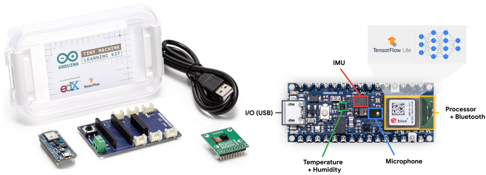](https://mlsysbook.ai/contents/core/ml_systems/images/png/tiny_ml.png "Figure 9: TinyML System Scale: These device kits exemplify the extreme miniaturization achievable with TinyML, enabling deployment of machine learning on resource-constrained devices with limited power and memory. such compact systems broaden the applicability of ML to previously inaccessible edge applications, including wearable sensors and embedded IoT devices. Source: [@warden2018speech]")
Figure 9: **TinyML System Scale**: These device kits exemplify the extreme miniaturization achievable with TinyML, enabling deployment of machine learning on resource-constrained devices with limited power and memory. such compact systems broaden the applicability of ML to previously inaccessible edge applications, including wearable sensors and embedded IoT devices. Source: ([Warden 2018](https://mlsysbook.ai/contents/core/ml_systems/ml_systems.html#ref-warden2018speech)
)
Warden, Pete. 2018. “Speech Commands: A Dataset for Limited-Vocabulary Speech Recognition.” _arXiv Preprint arXiv:1804.03209_, April. [https://doi.org/10.48550/arXiv.1804.03209](https://doi.org/10.48550/arXiv.1804.03209)
.
### TinyML Advantages and Operational Trade-offs
TinyML’s extreme resource constraints enable unique advantages impossible at other scales. Microsecond-level latency eliminates all transmission overhead, achieving 10-100μs response times that enable applications requiring sub-millisecond decisions: industrial vibration monitoring processes 10kHz sampling at under 50μs latency, audio wake-word detection analyzes 16kHz audio streams under 100μs, and precision manufacturing systems inspect over 1000 parts per minute. Economic advantages prove transformative for massive-scale deployments: complete ESP32-CAM systems cost $8-12, enabling 1000-sensor deployments for $10,000 versus $500,000-1,000,000 for cellular alternatives. Agricultural monitoring can instrument buildings for $5,000 versus $50,000+ for camera-based systems, while city-scale networks of 100,000 sensors become economically viable at $1-2 million versus $50-100 million for edge alternatives. Energy efficiency enables 1-10 year operation on coin-cell batteries consuming just 1-10mW, supporting applications like wildlife tracking for years without recapture, structural health monitoring embedded in concrete during construction, and agricultural sensors deployed where power infrastructure doesn’t exist. Energy harvesting from solar, vibration, or thermal sources can even enable perpetual operation. Privacy surpasses all other paradigms through physical data confinement—data never leaves the sensor, providing mathematical guarantees impossible in networked systems regardless of encryption strength.
These capabilities require substantial trade-offs. Computational constraints impose severe limits: microcontrollers provide 256KB-2MB RAM versus smartphones’ 12-24GB (a 5,000-50,000x difference), forcing models to remain under 100-500KB with 10,000-100,000 parameters compared to mobile’s 1-10 million parameters. Development complexity requires expertise spanning neural network optimization, hardware-level memory management, embedded toolchains, and specialized debugging using oscilloscopes and JTAG debuggers across diverse microcontroller architectures. Model accuracy suffers from extreme compression: TinyML models typically achieve 70-85% of cloud model accuracy versus mobile’s 90-95%, limiting suitability for applications requiring high precision. Deployment inflexibility constrains adaptation, as devices typically run single fixed models requiring power-intensive firmware flashing for updates that risk bricking devices. With operational lifetimes spanning years, initial deployment decisions become critical. Ecosystem fragmentation[39](https://mlsysbook.ai/contents/core/ml_systems/ml_systems.html#fn39)
across microcontroller vendors and ML frameworks creates substantial development overhead and platform lock-in challenges.
39 **TinyML Model Optimization**: Specialized techniques dramatically reduce model size. A typical 50MB smartphone model might optimize to 250KB for microcontroller deployment while retaining 95% accuracy (detailed in **[Chapter 10: Model Optimizations](https://mlsysbook.ai/contents/core/optimizations/optimizations.html#sec-model-optimizations)
**).
### Environmental and Health Monitoring
Tiny ML succeeds remarkably across domains where its unique advantages—ultra-low power, minimal cost, and complete data privacy—enable applications impossible with other paradigms. Industrial predictive maintenance demonstrates TinyML’s ability to transform traditional infrastructure through distributed intelligence. Manufacturing facilities deploy thousands of vibration sensors operating continuously for 5-10 years on coin-cell batteries while consuming less than 2mW average power. These sensors cost $15-50 compared to traditional wired sensors at $500-2,000 per point, reducing deployment costs from $5-20 million to $150,000-500,000 for 10,000 monitoring points. Local anomaly detection provides 7-14 day advance warning of equipment failures, enabling companies to achieve 25-45% reductions in unplanned downtime.
Wake-word detection represents TinyML’s most visible consumer application, with billions of devices employing always-listening capabilities at under 1mW continuous power consumption. These systems process 16kHz audio through neural networks containing 5,000-20,000 parameters compressed to 10-50KB, detecting wake phrases with over 95% accuracy. Amazon Echo devices use dedicated TinyML chips like the AML05 that consume less than 10mW for detection, only activating the main processor when wake words trigger—reducing average power consumption by 10-20x[40](https://mlsysbook.ai/contents/core/ml_systems/ml_systems.html#fn40)
.
40 **TinyML in Fitness Trackers**: Apple Watch detects falls using accelerometer data and on-device ML, automatically calling emergency services. The algorithm analyzes motion patterns in real-time using <1mW power.
Precision agriculture leverages TinyML’s economic advantages where traditional solutions prove cost-prohibitive. Monitoring 100 hectares requires approximately 1,000 monitoring points, which TinyML enables for $15,000-30,000 compared to $100,000-200,000+ for cellular-connected alternatives. These sensors operate 3-5 years on batteries while analyzing temporal patterns locally, transmitting only actionable insights rather than raw data streams.
Wildlife conservation demonstrates TinyML’s transformative potential for remote environmental monitoring. Researchers deploy solar-powered audio sensors consuming 100-500mW that process continuous audio streams for species identification. By performing local analysis, these systems reduce satellite transmission requirements from 4.3GB per day to 400KB of detection summaries, a 10,000x reduction that makes large-scale deployments of 100-1,000 sensors economically feasible. Medical wearables achieve FDA-cleared cardiac monitoring with 95-98% sensitivity while processing 250-500 ECG samples per second at under 5mW power consumption. This efficiency enables week-long continuous monitoring versus hours for smartphone-based alternatives, while reducing diagnostic costs from $2,000-5,000 for traditional in-lab studies to under $100 for at-home testing.
**Self-Check: Question 1.5**
1. Which of the following best describes a primary advantage of Tiny ML over Mobile ML?
1. Higher computational power
2. Increased data storage capacity
3. Greater model accuracy
4. Lower deployment cost and power consumption
2. Discuss the trade-offs involved in deploying Tiny ML systems in remote environments.
3. Tiny ML enables applications that require \_\_\_\_\_\_\_\_ decision making in resource-constrained environments.
4. True or False: Tiny ML systems can achieve the same level of model accuracy as cloud-based systems.
5. In a production system, which application is most suited for Tiny ML deployment?
1. Environmental monitoring
2. Real-time language translation
3. High-frequency stock trading
4. 3D rendering
[See Answers →](https://mlsysbook.ai/contents/core/ml_systems/ml_systems.html#quiz-answer-sec-ml-systems-tiny-ml-ubiquitous-sensing-scale-51d8)
Hybrid Architectures: Combining Paradigms
-----------------------------------------
Our examination of individual deployment paradigms—from cloud’s massive computational power to tiny ML’s ultra-efficient sensing—reveals a spectrum of engineering trade-offs, each with distinct advantages and limitations. Cloud ML maximizes algorithmic sophistication but introduces latency and privacy constraints. Edge ML reduces latency but requires dedicated infrastructure and constrains computational resources. Mobile ML prioritizes user experience but operates within strict battery and thermal limitations. Tiny ML achieves ubiquity through extreme efficiency but severely constrains model complexity. Each paradigm occupies a distinct niche, optimized for specific constraints and use cases.
Yet in practice, production systems rarely confine themselves to a single paradigm, as the limitations of each approach create opportunities for complementary integration. A voice assistant that uses tiny ML for wake-word detection, mobile ML for local speech recognition, edge ML for contextual processing, and cloud ML for complex natural language understanding demonstrates a more powerful approach. Hybrid Machine Learning formalizes this integration strategy, creating unified systems that leverage each paradigm’s complementary strengths while mitigating individual limitations.
**Definition:** Hybrid ML
**_Hybrid Machine Learning (Hybrid ML)_** is the integration of _multiple deployment paradigms_ into unified systems, strategically distributing workloads across _computational tiers_ to achieve _scalability_, _privacy_, and _performance_ impossible with single-paradigm approaches.
### Multi-Tier Integration Patterns
Hybrid ML design patterns provide reusable architectural solutions for integrating paradigms effectively. Each pattern represents a strategic approach to distributing ML workloads across computational tiers, optimized for specific trade-offs in latency, privacy, resource efficiency, and scalability.
This analysis identifies five essential patterns that address common integration challenges in hybrid ML systems.
#### Train-Serve Split
One of the most common hybrid patterns is the train-serve split, where model training occurs in the cloud but inference happens on edge, mobile, or tiny devices. This pattern takes advantage of the cloud’s vast computational resources for the training phase while benefiting from the low latency and privacy advantages of on-device inference[41](https://mlsysbook.ai/contents/core/ml_systems/ml_systems.html#fn41)
. For example, smart home devices often use models trained on large datasets in the cloud but run inference locally to ensure quick response times and protect user privacy. In practice, this might involve training models on powerful cloud systems like TPU Pods with exaflop-scale compute and hundreds of terabytes of memory, before deploying optimized versions to edge servers or embedded edge devices for efficient inference. Similarly, mobile vision models for computational photography are typically trained on powerful cloud infrastructure but deployed to run efficiently on phone hardware.
41 **Train-Serve Split Economics**: Training large models can cost $1-10M (GPT-3: $4.6M in compute costs) but inference costs <$0.01 per query when deployed efficiently ([Brown et al. 2020](https://mlsysbook.ai/contents/core/ml_systems/ml_systems.html#ref-brown2020language)
). This 1,000,000x cost difference drives the pattern of expensive cloud training with cost-effective edge inference.
Brown, Tom, Benjamin Mann, Nick Ryder, Melanie Subbiah, Jared D Kaplan, Prafulla Dhariwal, Arvind Neelakantan, et al. 2020. “Language Models Are Few-Shot Learners.” _Advances in Neural Information Processing Systems_ 33: 1877–1901. [https://proceedings.neurips.cc/paper/2020/file/1457c0d6bfcb4967418bfb8ac142f64a-Paper.pdf](https://proceedings.neurips.cc/paper/2020/file/1457c0d6bfcb4967418bfb8ac142f64a-Paper.pdf)
.
#### Hierarchical Processing
Hierarchical processing creates a multi-tier system where data and intelligence flow between different levels of the ML stack. This pattern effectively combines the capabilities of Cloud ML systems (like the large-scale training infrastructure discussed in previous sections) with multiple Edge ML systems (like edge servers and embedded devices from our edge deployment examples) to balance central processing power with local responsiveness. In industrial IoT applications, tiny sensors might perform basic anomaly detection, edge devices aggregate and analyze data from multiple sensors, and cloud systems handle complex analytics and model updates. For instance, we might see ESP32-CAM devices (from our Tiny ML examples) performing basic image classification at the sensor level with their minimal 520 KB RAM, feeding data up to edge servers or embedded systems for more sophisticated analysis, and ultimately connecting to cloud infrastructure for complex analytics and model updates.
This hierarchy allows each tier to handle tasks appropriate to its capabilities. Tiny ML devices handle immediate, simple decisions; edge devices manage local coordination; and cloud systems tackle complex analytics and learning tasks. Smart city installations often use this pattern, with street-level sensors feeding data to neighborhood-level edge processors, which in turn connect to city-wide cloud analytics.
#### Progressive Deployment
Progressive deployment creates tiered intelligence architectures by adapting models across computational tiers through systematic compression. A model might start as a large cloud version, then be progressively optimized for edge servers, mobile devices, and finally tiny sensors using techniques detailed in **[Chapter 10: Model Optimizations](https://mlsysbook.ai/contents/core/optimizations/optimizations.html#sec-model-optimizations)
**.
Amazon Alexa exemplifies this pattern: wake-word detection uses <1KB models on TinyML devices consuming <1mW, edge processing handles simple commands with 1-10MB models at 1-10W, while complex natural language understanding requires GB+ models in cloud infrastructure. This tiered approach reduces cloud inference costs by 95% while maintaining user experience.
However, progressive deployment introduces operational complexity: model versioning across tiers, ensuring consistency between generations, managing failure cascades during connectivity loss, and coordinating updates across millions of devices. Production teams must maintain specialized expertise spanning TinyML optimization, edge orchestration, and cloud scaling.
#### Federated Learning
Federated learning[42](https://mlsysbook.ai/contents/core/ml_systems/ml_systems.html#fn42)
enables learning from distributed data while maintaining privacy. Google’s production system processes 6 billion mobile keyboards, training improved models while keeping typed text local. Each training round involves 100-10,000 devices contributing model updates, requiring orchestration to manage device availability, network conditions, and computational heterogeneity.
42 **Federated Learning Architecture**: Coordinates learning across millions of devices without centralizing data ([McMahan et al. 2017](https://mlsysbook.ai/contents/core/ml_systems/ml_systems.html#ref-mcmahan2017federated)
). Google’s federated learning processes 6 billion mobile keyboards, training improved models while keeping all typed text local. Each round involves 100-10,000 devices contributing model updates.
McMahan, Brendan, Eider Moore, Daniel Ramage, Seth Hampson, and Blaise Agüera y Arcas. 2017. “Communication-Efficient Learning of Deep Networks from Decentralized Data.” In _Artificial Intelligence and Statistics_, 1273–82. PMLR. [http://proceedings.mlr.press/v54/mcmahan17a.html](http://proceedings.mlr.press/v54/mcmahan17a.html)
.
Production deployments face significant operational challenges: device dropout rates of 50-90% during training rounds, network bandwidth constraints limiting update frequency, and differential privacy mechanisms preventing information leakage. Aggregation servers must handle intermittent connectivity, varying device capabilities, and ensure convergence despite non-IID data distributions. This requires specialized monitoring infrastructure to track distributed training progress and debug issues without accessing raw data.
#### Collaborative Learning
Collaborative learning enables peer-to-peer learning between devices at the same tier, often complementing hierarchical structures.[43](https://mlsysbook.ai/contents/core/ml_systems/ml_systems.html#fn43)
Autonomous vehicle fleets, for example, might share learning about road conditions or traffic patterns directly between vehicles while also communicating with cloud infrastructure. This horizontal collaboration allows systems to share time-sensitive information and learn from each other’s experiences without always routing through central servers.
43 **Tiered Voice Processing**: Amazon Alexa uses a 3-tier system: tiny wake-word detection on-device (<1KB model), edge processing for simple commands (1-10MB models), and cloud processing for complex queries (GB+ models). This reduces cloud costs by 95% while maintaining functionality.
### Production System Case Studies
Real-world implementations integrate multiple design patterns into cohesive solutions rather than applying them in isolation. Production ML systems form interconnected networks where each paradigm plays a specific role while communicating with others, following integration patterns that leverage the strengths and address the limitations established in our four-paradigm framework ([Section 1.2](https://mlsysbook.ai/contents/core/ml_systems/ml_systems.html#sec-ml-systems-deployment-spectrum-38d0)
).
[Figure 10](https://mlsysbook.ai/contents/core/ml_systems/ml_systems.html#fig-hybrid)
illustrates these key interactions through specific connection types: “Deploy” paths show how models flow from cloud training to various devices, “Data” and “Results” show information flow from sensors through processing stages, “Analyze” shows how processed information reaches cloud analytics, and “Sync” demonstrates device coordination. Notice how data generally flows upward from sensors through processing layers to cloud analytics, while model deployments flow downward from cloud training to various inference points. The interactions aren’t strictly hierarchical. Mobile devices might communicate directly with both cloud services and tiny sensors, while edge systems can assist mobile devices with complex processing tasks.
[](https://mlsysbook.ai/contents/core/ml_systems/047b9fba8d702fcb8a171c8518556b1e6617c672.svg "Figure 10: Hybrid System Interactions: Data flows upward from sensors through processing layers to cloud analytics for insights, while trained models deploy downward from the cloud to enable inference at the edge, mobile, and Tiny ML devices. These connection types (deploy, data/results, analyze, and sync) establish a distributed architecture where each paradigm contributes unique capabilities to the overall machine learning system.")
Figure 10: **Hybrid System Interactions**: Data flows upward from sensors through processing layers to cloud analytics for insights, while trained models deploy downward from the cloud to enable inference at the edge, mobile, and Tiny ML devices. These connection types (deploy, data/results, analyze, and sync) establish a distributed architecture where each paradigm contributes unique capabilities to the overall machine learning system.
Production systems demonstrate these integration patterns across diverse applications where no single paradigm could deliver the required functionality. Industrial defect detection exemplifies model deployment patterns: cloud infrastructure trains vision models on datasets from multiple facilities, then distributes optimized versions to edge servers managing factory operations, tablets for quality inspectors, and embedded cameras on manufacturing equipment. This demonstrates how a single ML solution flows from centralized training to inference points at multiple computational scales.
Agricultural monitoring illustrates hierarchical data flow: soil sensors perform local anomaly detection, transmit results to edge processors that aggregate data from dozens of sensors, which then route insights to cloud infrastructure for farm-wide analytics while simultaneously updating farmers’ mobile applications. Information traverses upward through processing layers, with each tier adding analytical sophistication appropriate to its computational resources.
Fitness trackers exemplify gateway patterns between Tiny ML and mobile devices: wearables continuously monitor activity using algorithms optimized for microcontroller execution, sync processed data to smartphones that combine metrics from multiple sources, then transmit periodic updates to cloud infrastructure for long-term analysis. This enables tiny devices to participate in large-scale systems despite lacking direct network connectivity.
These integration patterns reveal how deployment paradigms complement each other through orchestrated data flows, model deployments, and cross-tier assistance. Industrial systems compose capabilities from Cloud, Edge, Mobile, and Tiny ML into distributed architectures that optimize for latency, privacy, cost, and operational requirements simultaneously. The interactions between paradigms often determine system success more than individual component capabilities.
**Self-Check: Question 1.6**
1. Which of the following best describes the primary advantage of using a hybrid ML architecture?
1. It maximizes computational efficiency by using only cloud resources.
2. It simplifies system design by focusing on a single deployment paradigm.
3. It allows for the integration of multiple paradigms to leverage their strengths.
4. It reduces the need for edge computing by relying on mobile devices.
2. True or False: In a hybrid ML system, the train-serve split pattern is used to perform both training and inference on edge devices to maximize efficiency.
3. Explain how hierarchical processing in hybrid ML systems balances central processing power with local responsiveness.
4. Order the following steps in a federated learning process: (1) Aggregation of model updates, (2) Local model training on devices, (3) Distribution of global model to devices.
5. In a production system, what are the potential challenges of implementing progressive deployment in hybrid ML architectures?
[See Answers →](https://mlsysbook.ai/contents/core/ml_systems/ml_systems.html#quiz-answer-sec-ml-systems-hybrid-architectures-combining-paradigms-c1f2)
Shared Principles Across Deployment Paradigms
---------------------------------------------
Despite their diversity, all ML deployment paradigms share core principles that enable systematic understanding and effective hybrid combinations. [Figure 11](https://mlsysbook.ai/contents/core/ml_systems/ml_systems.html#fig-ml-systems-convergence)
illustrates how implementations spanning cloud to tiny devices converge on core system challenges: managing data pipelines, balancing resource constraints, and implementing reliable architectures. This convergence explains why techniques transfer effectively between paradigms and hybrid approaches work successfully in practice.
[](https://mlsysbook.ai/contents/core/ml_systems/5fedc48a7e99a893f124b30012db0e32753613d4.svg "Figure 11: Convergence of ML Systems: Diverse machine learning deployments (cloud, edge, mobile, and tiny) share foundational principles in data pipelines, resource management, and system architecture, enabling hybrid solutions and systematic design approaches. Understanding these shared principles allows practitioners to adapt techniques across different paradigms and build cohesive, efficient ML workflows despite varying constraints and optimization goals.")
Figure 11: **Convergence of ML Systems**: Diverse machine learning deployments (cloud, edge, mobile, and tiny) share foundational principles in data pipelines, resource management, and system architecture, enabling hybrid solutions and systematic design approaches. Understanding these shared principles allows practitioners to adapt techniques across different paradigms and build cohesive, efficient ML workflows despite varying constraints and optimization goals.
[Figure 11](https://mlsysbook.ai/contents/core/ml_systems/ml_systems.html#fig-ml-systems-convergence)
reveals three distinct layers of abstraction that unify ML system design across deployment contexts.
The top layer represents ML system implementations—the four deployment paradigms examined throughout this chapter. Cloud ML operates in data centers with training at scale, Edge ML performs local processing focused on inference, Mobile ML runs on personal devices for user applications, and TinyML executes on embedded systems under severe resource constraints. Despite their apparent differences, these implementations share deeper commonalities that emerge in the underlying layers.
The middle layer identifies core system principles that unite all paradigms. Data pipeline management (**[Chapter 6: Data Engineering](https://mlsysbook.ai/contents/core/data_engineering/data_engineering.html#sec-data-engineering)
**) governs information flow from collection through deployment, maintaining consistent patterns whether processing petabytes in cloud data centers or kilobytes on microcontrollers. Resource management creates universal challenges in balancing competing demands for computation, memory, energy, and network capacity across all scales. System architecture principles guide the integration of models, hardware, and software components regardless of deployment context. These foundational principles remain remarkably consistent even as implementations vary by orders of magnitude in available resources.
The bottom layer shows how system considerations manifest these principles across practical dimensions. Optimization and efficiency strategies (**[Chapter 10: Model Optimizations](https://mlsysbook.ai/contents/core/optimizations/optimizations.html#sec-model-optimizations)
**) take different forms at each scale: cloud GPU cluster training, edge model compression, mobile thermal management, and TinyML numerical precision, yet all pursue maximizing performance within available resources. Operational aspects (**[Chapter 13: ML Operations](https://mlsysbook.ai/contents/core/ops/ops.html#sec-ml-operations)
**) address deployment, monitoring, and updates with paradigm-specific approaches that tackle fundamentally similar challenges. Trustworthy AI (**[Chapter 17: Responsible AI](https://mlsysbook.ai/contents/core/responsible_ai/responsible_ai.html#sec-responsible-ai)
**, **[Chapter 16: Robust AI](https://mlsysbook.ai/contents/core/robust_ai/robust_ai.html#sec-robust-ai)
**) requirements for security, privacy, and reliability apply universally, though implementation techniques necessarily adapt to each deployment context.
This three-layer structure explains why techniques transfer effectively between scales. Cloud-trained models deploy successfully to edge devices because training and inference optimize similar objectives under different constraints. Mobile optimization insights inform cloud efficiency strategies because both manage the same fundamental resource trade-offs. TinyML innovations drive cross-paradigm advances precisely because extreme constraints force solutions to core problems that exist at all scales. Hybrid approaches work effectively (train-serve splits, hierarchical processing, federated learning) because underlying principles align across paradigms, enabling seamless integration despite vast differences in available resources.
**Self-Check: Question 1.7**
1. Which of the following best describes why different ML deployment paradigms (cloud, edge, mobile, tiny) can effectively share techniques?
1. They all operate under the same resource constraints.
2. They focus exclusively on inference tasks.
3. They all use the same hardware components.
4. They share core principles such as data pipeline management and resource management.
2. True or False: The convergence of ML system designs across different deployment paradigms is primarily due to similar hardware architectures.
3. Explain how understanding core system principles can aid in the development of hybrid ML systems.
4. The three layers of abstraction in ML system design are implementations, core system principles, and \_\_\_\_.
5. Order the following ML system layers from top to bottom based on their role in design abstraction: (1) System Considerations, (2) Implementations, (3) Core System Principles.
[See Answers →](https://mlsysbook.ai/contents/core/ml_systems/ml_systems.html#quiz-answer-sec-ml-systems-shared-principles-across-deployment-paradigms-915d)
Comparative Analysis and Selection Framework
--------------------------------------------
Building from this understanding of shared principles, systematic comparison across deployment paradigms reveals the precise trade-offs that should drive deployment decisions and highlights scenarios where each paradigm excels, providing practitioners with analytical frameworks for making informed architectural choices.
The relationship between computational resources and deployment location forms one of the most important comparisons across ML systems. As we move from cloud deployments to tiny devices, we observe a dramatic reduction in available computing power, storage, and energy consumption. Cloud ML systems, with their data center infrastructure, can leverage virtually unlimited resources, processing data at the scale of petabytes and training models with billions of parameters. Edge ML systems, while more constrained, still offer significant computational capability through specialized hardware like edge GPUs and neural processing units. Mobile ML represents a middle ground, balancing computational power with energy efficiency on devices like smartphones and tablets. At the far end of the spectrum, TinyML operates under severe resource constraints, often limited to kilobytes of memory and milliwatts of power consumption.
Table 2: **Deployment Locations**: Machine learning systems vary in where computation occurs, from centralized cloud servers to local edge devices and ultra-low-power TinyML chips, each impacting latency, bandwidth, and energy consumption. This table categorizes these deployments by their processing location and associated characteristics, enabling informed decisions about system architecture and resource allocation.
| | | | | |
| --- | --- | --- | --- | --- |
| **Performance** | | | | |
| **Processing Location** | Centralized cloud servers (Data Centers) | Local edge devices (gateways, servers) | Smartphones and tablets | Ultra-low-power microcontrollers and embedded systems |
| **Latency** | High (100 ms-1000 ms+) | Moderate (10-100 ms) | Low-Moderate (5-50 ms) | Very Low (1-10 ms) |
| **Compute Power** | Very High (Multiple GPUs/TPUs) | High (Edge GPUs) | Moderate (Mobile NPUs/GPUs) | Very Low (MCU/tiny processors) |
| **Storage Capacity** | Unlimited (petabytes+) | Large (terabytes) | Moderate (gigabytes) | Very Limited (kilobytes-megabytes) |
| **Energy Consumption** | Very High (kW-MW range) | High (100 s W) | Moderate (1-10 W) | Very Low (mW range) |
| **Scalability** | Excellent (virtually unlimited) | Good (limited by edge hardware) | Moderate (per-device scaling) | Limited (fixed hardware) |
| **Operational** | | | | |
| **Data Privacy** | Basic-Moderate (Data leaves device) | High (Data stays in local network) | High (Data stays on phone) | Very High (Data never leaves sensor) |
| **Connectivity Required** | Constant high-bandwidth | Intermittent | Optional | None |
| **Offline Capability** | None | Good | Excellent | Complete |
| **Real-time Processing** | Dependent on network | Good | Very Good | Excellent |
| **Deployment** | | | | |
| **Cost** | High ($1000s+/month) | Moderate ($100s-1000s) | Low ($0-10s) | Very Low ($1-10s) |
| **Hardware Requirements** | Cloud infrastructure | Edge servers/gateways | Modern smartphones | MCUs/embedded systems |
| **Development Complexity** | High (cloud expertise needed) | Moderate-High (edge+networking) | Moderate (mobile SDKs) | High (embedded expertise) |
| **Deployment Speed** | Fast | Moderate | Fast | Slow |
[Table 2](https://mlsysbook.ai/contents/core/ml_systems/ml_systems.html#tbl-big_vs_tiny)
quantifies these paradigm differences across performance, operational, and deployment dimensions, revealing clear gradients in latency (cloud: 100-1000ms → edge: 10-100ms → mobile: 5-50ms → tiny: 1-10ms) and privacy guarantees (strongest with TinyML’s complete local processing).
[Figure 12](https://mlsysbook.ai/contents/core/ml_systems/ml_systems.html#fig-op_char)
visualizes performance and operational characteristics through radar plots. Plot a) contrasts compute power and scalability (Cloud ML’s strengths) against latency and energy efficiency (TinyML’s advantages), with Edge and Mobile ML occupying intermediate positions.
[](https://mlsysbook.ai/contents/core/ml_systems/bc71b7cb86d1a14fb63efcb143e44ef94bdea315.svg "Figure 12: ML System Trade-Offs: Radar plots quantify performance and operational characteristics across cloud, edge, mobile, and Tiny ML paradigms, revealing inherent trade-offs between compute power, latency, energy consumption, and scalability. These visualizations enable informed selection of the most suitable deployment approach based on application-specific constraints and priorities.")
Figure 12: **ML System Trade-Offs**: Radar plots quantify performance and operational characteristics across cloud, edge, mobile, and Tiny ML paradigms, revealing inherent trade-offs between compute power, latency, energy consumption, and scalability. These visualizations enable informed selection of the most suitable deployment approach based on application-specific constraints and priorities.
Plot b) emphasizes operational dimensions where TinyML excels (privacy, connectivity independence, offline capability) versus Cloud ML’s dependency on centralized infrastructure and constant connectivity.
Development complexity varies inversely with hardware capability: Cloud and TinyML require deep expertise (cloud infrastructure and embedded systems respectively), while Mobile and Edge leverage more accessible SDKs and tooling. Cost structures show similar inversion: Cloud incurs ongoing operational expenses ($1000s+/month), Edge requires moderate upfront investment ($100s-1000s), Mobile leverages existing devices ($0-10s), and TinyML minimizes hardware costs ($1-10s) while demanding higher development investment.
Understanding these trade-offs proves crucial for selecting appropriate deployment strategies that align application requirements with paradigm capabilities.
A critical pitfall in deployment selection involves choosing paradigms based solely on model accuracy metrics without considering system-level constraints. Teams often select deployment strategies by comparing model accuracy in isolation, overlooking critical system requirements that determine real-world viability. A cloud-deployed model achieving 99% accuracy becomes useless for autonomous emergency braking if network latency exceeds reaction time requirements. Similarly, a sophisticated edge model that drains a mobile device’s battery in minutes fails despite superior accuracy. Successful deployment requires evaluating multiple dimensions simultaneously: latency requirements, power budgets, network reliability, data privacy regulations, and total cost of ownership. Establish these constraints before model development to avoid expensive architectural pivots late in the project.
**Self-Check: Question 1.8**
1. Which deployment paradigm offers the highest data privacy due to local processing?
1. Cloud ML
2. Edge ML
3. Mobile ML
4. Tiny ML
2. Discuss the trade-offs between energy consumption and computational power when selecting a deployment paradigm for an ML system.
3. In a scenario where low latency and offline capability are critical, which deployment paradigm is most suitable?
1. Cloud ML
2. Tiny ML
3. Mobile ML
4. Edge ML
4. How might you apply the understanding of deployment paradigm trade-offs in your own ML project?
[See Answers →](https://mlsysbook.ai/contents/core/ml_systems/ml_systems.html#quiz-answer-sec-ml-systems-comparative-analysis-selection-framework-832e)
Decision Framework for Deployment Selection
-------------------------------------------
Selecting the appropriate deployment paradigm requires systematic evaluation of application constraints rather than organizational biases or technology trends. [Figure 13](https://mlsysbook.ai/contents/core/ml_systems/ml_systems.html#fig-mlsys-playbook-flowchart)
provides a hierarchical decision framework that filters options through critical requirements: privacy (can data leave the device?), latency (sub-10ms response needed?), computational demands (heavy processing required?), and cost constraints (budget limitations?). This structured approach ensures deployment decisions emerge from application requirements, grounded in the physical constraints ([Section 1.2.1](https://mlsysbook.ai/contents/core/ml_systems/ml_systems.html#sec-ml-systems-deployment-paradigm-foundations-0c17)
) and quantitative comparisons ([Section 1.9](https://mlsysbook.ai/contents/core/ml_systems/ml_systems.html#sec-ml-systems-comparative-analysis-selection-framework-832e)
) established earlier.
[](https://mlsysbook.ai/contents/core/ml_systems/216fb8731d81432c618b0b4e7b8e1c1ac3ec6537.svg "Figure 13: Deployment Decision Logic: This flowchart guides selection of an appropriate machine learning deployment paradigm by systematically evaluating privacy requirements and processing constraints, ultimately balancing performance, cost, and data security. Navigating the decision tree helps practitioners determine whether cloud, edge, mobile, or tiny machine learning best suits a given application.")
Figure 13: **Deployment Decision Logic**: This flowchart guides selection of an appropriate machine learning deployment paradigm by systematically evaluating privacy requirements and processing constraints, ultimately balancing performance, cost, and data security. Navigating the decision tree helps practitioners determine whether cloud, edge, mobile, or tiny machine learning best suits a given application.
The framework evaluates four critical decision layers sequentially. Privacy constraints form the first filter, determining whether data can be transmitted externally. Applications handling sensitive data under GDPR, HIPAA, or proprietary restrictions mandate local processing, immediately eliminating cloud-only deployments. Latency requirements establish the second constraint through response time budgets: applications requiring sub-10ms response times cannot use cloud processing, as physics-imposed network delays alone exceed this threshold. Computational demands form the third evaluation layer, assessing whether applications require high-performance infrastructure that only cloud or edge systems provide, or whether they can operate within the resource constraints of mobile or tiny devices. Cost considerations complete the framework by balancing capital expenditure, operational expenses, and energy efficiency across expected deployment lifetimes.
Technical constraints alone prove insufficient for deployment decisions. Organizational factors critically shape success by determining whether teams possess the capabilities to implement and maintain chosen paradigms. Team expertise must align with paradigm requirements: Cloud ML demands distributed systems knowledge, Edge ML requires device management capabilities, Mobile ML needs platform-specific optimization skills, and TinyML requires embedded systems expertise. Organizations lacking appropriate skills face extended development timelines and ongoing maintenance challenges that undermine technical advantages. Monitoring and maintenance capabilities similarly determine viability at scale: edge deployments require distributed device orchestration, while TinyML demands specialized firmware management that many organizations lack. Cost structures further complicate decisions through their temporal patterns: Cloud incurs recurring operational expenses favorable for unpredictable workloads, Edge requires substantial upfront investment offset by lower ongoing costs, Mobile leverages user-provided devices to minimize infrastructure expenses, and TinyML minimizes hardware and connectivity costs while demanding significant development investment.
Successful deployment emerges from balancing technical optimization against organizational capability. Paradigm selection represents systems engineering challenges that extend well beyond pure technical requirements, encompassing team skills, operational capacity, and economic constraints. These decisions remain constrained by fundamental scaling laws explored in **[AI Scaling Laws](https://mlsysbook.ai/contents/core/efficient_ai/efficient_ai.html#sec-efficient-ai-ai-scaling-laws-a043)
**, with operational aspects detailed in **[Chapter 13: ML Operations](https://mlsysbook.ai/contents/core/ops/ops.html#sec-ml-operations)
** and benchmarking approaches covered in **[Chapter 12: Benchmarking AI](https://mlsysbook.ai/contents/core/benchmarking/benchmarking.html#sec-benchmarking-ai)
**.
**Self-Check: Question 1.9**
1. Which of the following is the first criterion evaluated in the deployment decision framework?
1. Latency requirements
2. Computational demands
3. Cost constraints
4. Privacy constraints
2. Explain why latency requirements are a critical factor in the deployment decision framework.
3. In the deployment decision framework, applications with significant computational demands are best suited for \_\_\_\_\_\_\_\_ or edge systems.
4. Order the following decision criteria in the deployment framework: (1) Cost constraints, (2) Privacy constraints, (3) Computational demands, (4) Latency requirements.
5. In a production system, how might organizational factors influence the choice of deployment paradigm?
[See Answers →](https://mlsysbook.ai/contents/core/ml_systems/ml_systems.html#quiz-answer-sec-ml-systems-decision-framework-deployment-selection-f748)
Fallacies and Pitfalls
----------------------
Understanding deployment paradigms requires recognizing common misconceptions that can lead to poor architectural decisions. These fallacies often stem from oversimplified thinking about the core trade-offs governing ML systems design.
**Fallacy: “One Paradigm Fits All”** - The most pervasive misconception assumes that one deployment approach can solve all ML problems. Teams often standardize on cloud, edge, or mobile solutions without considering application-specific constraints. This fallacy ignores the physics-imposed boundaries discussed in [Section 1.2.1](https://mlsysbook.ai/contents/core/ml_systems/ml_systems.html#sec-ml-systems-deployment-paradigm-foundations-0c17)
. Real-time robotics cannot tolerate cloud latency, while complex language models exceed tiny device capabilities. Effective systems often require hybrid architectures that leverage multiple paradigms strategically.
**Fallacy: “Edge Computing Always Reduces Latency”** - Many practitioners assume edge deployment automatically improves response times. However, edge systems introduce processing delays, load balancing overhead, and potential network hops that can exceed direct cloud connections. A poorly designed edge deployment with insufficient local compute power may exhibit worse latency than optimized cloud services. Edge benefits emerge only when local processing time plus reduced network distance outweighs the infrastructure complexity costs.
**Fallacy: “Mobile Devices Can Handle Any Workload with Optimization”** - This misconception underestimates the fundamental constraints imposed by battery life and thermal management. Teams often assume that model compression techniques can arbitrarily reduce resource requirements while maintaining performance. However, mobile devices face hard physical limits: battery capacity scales with volume while computational demand scales with model complexity. Some applications require computational resources that no amount of optimization can fit within mobile power budgets.
**Fallacy: “Tiny ML is Just Smaller Mobile ML”** - This fallacy misunderstands the qualitative differences between resource-constrained paradigms. Tiny ML operates under constraints so severe that different algorithmic approaches become necessary. The microcontroller environments impose memory limitations measured in kilobytes, not megabytes, requiring specialized techniques like quantization beyond what mobile optimization employs. Applications suitable for tiny ML represent a fundamentally different problem class, not simply scaled-down versions of mobile applications.
**Fallacy: “Cost Optimization Equals Resource Minimization”** - Teams frequently assume that minimizing computational resources automatically reduces costs. This perspective ignores operational complexity, development time, and infrastructure overhead. Cloud deployments may consume more compute resources while providing lower total cost of ownership through reduced maintenance, automatic scaling, and shared infrastructure. The optimal cost solution often involves accepting higher per-unit resource consumption in exchange for simplified operations and faster development cycles.
**Self-Check: Question 1.10**
1. Which of the following statements is a common misconception about ML deployment paradigms?
1. One deployment approach can solve all ML problems.
2. Edge computing always reduces latency.
3. All of the above.
4. Mobile devices can handle any workload with optimization.
2. True or False: Edge computing always results in reduced latency compared to cloud computing.
3. Explain why the fallacy ‘Cost Optimization Equals Resource Minimization’ can lead to suboptimal ML system designs.
4. Why might a hybrid ML architecture be necessary despite the fallacy that ‘One Paradigm Fits All’?
1. To minimize the use of computational resources.
2. To avoid the complexities of cloud-based solutions.
3. To simplify the deployment process.
4. To leverage the strengths of multiple deployment paradigms.
[See Answers →](https://mlsysbook.ai/contents/core/ml_systems/ml_systems.html#quiz-answer-sec-ml-systems-fallacies-pitfalls-8074)
Summary
-------
This chapter analyzed the diverse landscape of machine learning systems, revealing how deployment context directly shapes every aspect of system design. From cloud environments with vast computational resources to tiny devices operating under extreme constraints, each paradigm presents unique opportunities and challenges that directly influence architectural decisions, algorithmic choices, and performance trade-offs. The spectrum from cloud to edge to mobile to tiny ML represents more than just different scales of computation; it reflects a significant evolution in how we distribute intelligence across computing infrastructure.
The evolution from centralized cloud systems to distributed edge and mobile deployments shows how resource constraints drive innovation rather than simply limiting capabilities. Each paradigm emerged to address specific limitations of its predecessors: Cloud ML leverages centralized power for complex processing but must navigate latency and privacy concerns. Edge ML brings computation closer to data sources, reducing latency while introducing intermediate resource constraints. Mobile ML extends these capabilities to personal devices, balancing user experience with battery life and thermal management. Tiny ML pushes the boundaries of what’s possible with minimal resources, enabling ubiquitous sensing and intelligence in previously impossible deployment contexts. This evolution showcases how thoughtful system design can transform limitations into opportunities for specialized optimization.
Key Takeaways
* Deployment context drives architectural decisions more than algorithmic preferences
* Resource constraints create opportunities for innovation, not just limitations
* Hybrid approaches are emerging as the future of ML system design
* Privacy and latency considerations increasingly favor distributed intelligence
These paradigms reflect an ongoing shift toward systems that are finely tuned to specific operational requirements, moving beyond one-size-fits-all approaches toward context-aware system design. As these deployment models mature, hybrid architectures emerge that combine their strengths: cloud-based training paired with edge inference, federated learning across mobile devices, and hierarchical processing that optimizes across the entire spectrum. This evolution demonstrates how deployment contexts will continue driving innovation in system architecture, training methodologies, and optimization techniques, creating more sophisticated and context-aware ML systems.
Yet deployment context represents only one dimension of system design. The algorithms executing within these environments equally influence resource requirements, computational patterns, and optimization strategies. A neural network requiring gigabytes of memory and billions of floating-point operations demands fundamentally different deployment approaches than a decision tree requiring kilobytes and integer comparisons. The next chapter (**[Chapter 3: Deep Learning Primer](https://mlsysbook.ai/contents/core/dl_primer/dl_primer.html#sec-dl-primer)
**) examines the mathematical foundations of neural networks, revealing why certain deployment paradigms suit specific algorithms and how algorithmic choices propagate through the entire system stack.
**Self-Check: Question 1.11**
1. Which of the following best describes the primary reason why deployment context drives architectural decisions in ML systems?
1. Algorithmic preferences are more important than deployment context.
2. Deployment context is irrelevant to ML system design.
3. Deployment context dictates resource availability and constraints.
4. Deployment context only affects data privacy concerns.
2. Explain how resource constraints can drive innovation in ML system design, using the evolution from cloud to tiny ML as an example.
3. Which deployment paradigm is most likely to prioritize battery life and thermal management?
1. Cloud ML
2. Mobile ML
3. Edge ML
4. Tiny ML
4. Discuss the potential benefits of hybrid ML architectures that combine cloud-based training with edge inference.
[See Answers →](https://mlsysbook.ai/contents/core/ml_systems/ml_systems.html#quiz-answer-sec-ml-systems-summary-473b)
Self-Check Answers
------------------
**Self-Check: Answer 1.1**
1. **Which of the following best describes the impact of deployment environments on machine learning system architecture?**
1. Deployment environments have no significant impact on system architecture.
2. Deployment environments dictate the choice of algorithms used in ML systems.
3. Deployment environments shape architectural decisions based on operational constraints.
4. Deployment environments only affect the hardware used in ML systems.
_Answer_: The correct answer is C. Deployment environments shape architectural decisions based on operational constraints. This is correct because the section emphasizes how different environments, such as cloud or mobile, impose specific requirements that influence system design.
_Learning Objective_: Understand how deployment environments influence architectural decisions in ML systems.
2. **Explain how the deployment environment for a mobile device might influence the architectural design of a machine learning system.**
_Answer_: In a mobile deployment environment, architectural design must prioritize latency and power efficiency due to limited computational resources and battery life. For example, real-time object detection on a mobile device requires optimizing algorithms to run efficiently without draining the battery. This is important because it ensures the system remains responsive and usable in a mobile context.
_Learning Objective_: Analyze how specific deployment environments impact architectural design in ML systems.
3. **Which deployment paradigm is most suitable for applications requiring ultra-low latency and privacy?**
1. Cloud computing
2. Tiny machine learning
3. Mobile computing
4. Edge computing
_Answer_: The correct answer is D. Edge computing. This is correct because edge computing positions computation close to data sources, minimizing latency and enhancing privacy by processing data locally.
_Learning Objective_: Identify suitable deployment paradigms based on specific operational requirements.
4. **True or False: Hybrid architectures in machine learning systems only use cloud-based resources to optimize performance.**
_Answer_: False. Hybrid architectures strategically allocate tasks across multiple paradigms, including edge and mobile computing, to optimize system-wide performance, not just cloud resources.
_Learning Objective_: Understand the role of hybrid architectures in optimizing ML system performance.
5. **In a production system, which deployment paradigm would likely be used for a factory automation application prioritizing power efficiency and deterministic response times?**
1. Tiny machine learning
2. Edge computing
3. Mobile computing
4. Cloud computing
_Answer_: The correct answer is A. Tiny machine learning. This is correct because tiny machine learning focuses on energy efficiency and can operate on resource-constrained devices, making it suitable for factory automation where power efficiency and deterministic response times are critical.
_Learning Objective_: Apply knowledge of deployment paradigms to real-world ML system scenarios.
[← Back to Questions](https://mlsysbook.ai/contents/core/ml_systems/ml_systems.html#quiz-question-sec-ml-systems-deployment-spectrum-38d0)
**Self-Check: Answer 1.2**
1. **Which of the following is a primary advantage of using Cloud ML for machine learning tasks?**
1. Immense computational power
2. Enhanced data privacy
3. Reduced network latency
4. Lower initial hardware costs
_Answer_: The correct answer is A. Immense computational power. Cloud ML provides substantial computational resources, making it suitable for large-scale data processing and complex model training. Options B and C are incorrect because cloud ML typically involves higher latency and potential privacy concerns. Option D is misleading as cloud ML can be cost-effective but involves ongoing operational costs.
_Learning Objective_: Understand the primary advantages of Cloud ML in handling computationally intensive tasks.
2. **Discuss the trade-offs involved in deploying machine learning models on cloud infrastructure.**
_Answer_: Deploying ML models on cloud infrastructure offers scalability and computational power but introduces trade-offs such as latency, data privacy concerns, and operational costs. For example, cloud ML is unsuitable for real-time applications due to network delays. This is important because organizations must balance these trade-offs against their specific application requirements.
_Learning Objective_: Analyze the trade-offs associated with cloud ML deployment, including latency and cost considerations.
3. **True or False: Cloud ML is always the best choice for machine learning applications due to its superior computational power.**
_Answer_: False. While Cloud ML offers significant computational power, it is not always the best choice due to trade-offs like latency, privacy concerns, and cost. The optimal deployment depends on specific application requirements.
_Learning Objective_: Challenge the misconception that Cloud ML is universally superior by understanding its limitations.
4. **Order the following cloud ML characteristics by their impact on deployment decisions: (1) Latency, (2) Computational Power, (3) Cost, (4) Data Privacy.**
_Answer_: The correct order is: (2) Computational Power, (1) Latency, (4) Data Privacy, (3) Cost. Computational power is often the primary reason for choosing cloud ML, but latency and privacy concerns can significantly impact deployment decisions. Cost considerations come into play when evaluating long-term operational expenses.
_Learning Objective_: Understand the relative impact of different cloud ML characteristics on deployment decisions.
[← Back to Questions](https://mlsysbook.ai/contents/core/ml_systems/ml_systems.html#quiz-question-sec-ml-systems-cloud-ml-maximizing-computational-power-f232)
**Self-Check: Answer 1.3**
1. **Which of the following best describes a primary advantage of Edge ML over Cloud ML for latency-critical applications?**
1. Unlimited computational resources
2. Reduced latency
3. Lower initial deployment costs
4. Enhanced data transmission capabilities
_Answer_: The correct answer is B. Reduced latency. This is correct because Edge ML processes data locally, eliminating the network round-trip time inherent in cloud processing, which is crucial for latency-critical applications. Options A, C, and D do not directly address latency improvements.
_Learning Objective_: Understand the latency benefits of Edge ML compared to Cloud ML.
2. **True or False: Edge ML inherently provides better data privacy than Cloud ML.**
_Answer_: True. This is true because Edge ML processes data locally, reducing the need to transmit sensitive information over networks, which enhances privacy by minimizing exposure to potential breaches during transmission.
_Learning Objective_: Evaluate privacy advantages of Edge ML over Cloud ML.
3. **Discuss the trade-offs between computational resources and latency when choosing between Cloud ML and Edge ML for a real-time industrial IoT application.**
_Answer_: Edge ML offers reduced latency, crucial for real-time applications, by processing data locally. However, it sacrifices the extensive computational resources available in cloud environments, limiting model complexity. For industrial IoT, this trade-off means prioritizing quick decision-making over model sophistication. This is important because real-time responsiveness can significantly impact operational efficiency and safety.
_Learning Objective_: Analyze the trade-offs in computational resources and latency for real-time applications.
4. **Edge ML systems typically operate in the tens to hundreds of watts range and rely on localized hardware optimized for \_\_\_\_ processing.**
_Answer_: real-time. Edge ML systems are designed to process data quickly and locally, reducing latency compared to cloud-based systems.
_Learning Objective_: Recall key characteristics of Edge ML systems.
5. **Order the following Edge ML benefits by their impact on deployment decisions: (1) Enhanced Data Privacy, (2) Reduced Latency, (3) Lower Bandwidth Usage.**
_Answer_: The correct order is: (2) Reduced Latency, (1) Enhanced Data Privacy, (3) Lower Bandwidth Usage. Reduced latency is often the most critical factor for real-time applications, followed by privacy concerns, especially in regulated industries. Bandwidth usage, while significant, is typically a secondary consideration.
_Learning Objective_: Prioritize Edge ML benefits based on their impact on deployment decisions.
[← Back to Questions](https://mlsysbook.ai/contents/core/ml_systems/ml_systems.html#quiz-question-sec-ml-systems-edge-ml-reducing-latency-privacy-risk-31f9)
**Self-Check: Answer 1.4**
1. **Which of the following best describes a primary advantage of Mobile ML over Edge ML?**
1. Greater computational power
2. Improved user privacy and offline functionality
3. Reduced hardware costs
4. Higher data storage capacity
_Answer_: The correct answer is B. Improved user privacy and offline functionality. Mobile ML allows on-device processing, enhancing privacy and enabling offline use, which is crucial for personal and responsive applications.
_Learning Objective_: Understand the primary advantages of Mobile ML in terms of privacy and offline capabilities.
2. **Discuss the trade-offs involved in deploying machine learning models on mobile devices compared to cloud-based systems.**
_Answer_: Deploying ML models on mobile devices offers benefits like enhanced privacy and offline functionality but comes with trade-offs such as limited computational resources, battery life constraints, and storage limitations. For example, mobile devices must optimize models to fit within their power and thermal constraints, unlike cloud systems that can handle larger models and more intensive computations. This is important because it affects the design and deployment strategies for mobile ML applications.
_Learning Objective_: Analyze the trade-offs between deploying ML models on mobile devices versus cloud systems.
3. **True or False: Mobile ML can achieve the same level of computational sophistication as cloud-based ML systems.**
_Answer_: False. Mobile ML operates under strict power and thermal constraints, limiting its computational resources compared to cloud-based systems, which can support larger and more complex models.
_Learning Objective_: Recognize the computational limitations of Mobile ML compared to cloud-based systems.
4. **In a production system, which application is most suited for Mobile ML deployment?**
1. Real-time voice recognition
2. Large-scale data analytics
3. Complex neural network training
4. Batch processing of large datasets
_Answer_: The correct answer is A. Real-time voice recognition. Mobile ML excels in applications requiring immediate responsiveness and privacy, such as real-time voice recognition on smartphones.
_Learning Objective_: Identify suitable applications for Mobile ML deployment based on system constraints and capabilities.
[← Back to Questions](https://mlsysbook.ai/contents/core/ml_systems/ml_systems.html#quiz-question-sec-ml-systems-mobile-ml-personal-offline-intelligence-7905)
**Self-Check: Answer 1.5**
1. **Which of the following best describes a primary advantage of Tiny ML over Mobile ML?**
1. Higher computational power
2. Increased data storage capacity
3. Greater model accuracy
4. Lower deployment cost and power consumption
_Answer_: The correct answer is D. Lower deployment cost and power consumption. Tiny ML devices are designed to operate with minimal resources, making them cost-effective and energy-efficient compared to Mobile ML systems, which require more sophisticated hardware.
_Learning Objective_: Understand the primary advantages of Tiny ML in terms of cost and power efficiency.
2. **Discuss the trade-offs involved in deploying Tiny ML systems in remote environments.**
_Answer_: Deploying Tiny ML systems in remote environments involves trade-offs such as limited computational resources and model accuracy against benefits like ultra-low power consumption and cost-effectiveness. These systems can operate autonomously for years, but their constrained resources may limit the complexity and accuracy of the models they run. For example, Tiny ML systems are ideal for applications like environmental monitoring where long-term operation and data privacy are prioritized over high precision.
_Learning Objective_: Analyze the trade-offs of deploying Tiny ML in resource-constrained environments.
3. **Tiny ML enables applications that require \_\_\_\_\_\_\_\_ decision making in resource-constrained environments.**
_Answer_: localized. Tiny ML allows for decision making directly on the device without relying on external data processing, which is crucial in environments with limited connectivity.
_Learning Objective_: Recall the concept of localized decision making in Tiny ML systems.
4. **True or False: Tiny ML systems can achieve the same level of model accuracy as cloud-based systems.**
_Answer_: False. Tiny ML systems typically achieve 70-85% of cloud model accuracy due to their extreme resource constraints, which limit the complexity of the models they can run.
_Learning Objective_: Understand the limitations of Tiny ML in terms of model accuracy compared to cloud-based systems.
5. **In a production system, which application is most suited for Tiny ML deployment?**
1. Environmental monitoring
2. Real-time language translation
3. High-frequency stock trading
4. 3D rendering
_Answer_: The correct answer is A. Environmental monitoring. Tiny ML is well-suited for applications like environmental monitoring that require long-term, low-power operation in remote areas, where data privacy and cost-effectiveness are critical.
_Learning Objective_: Identify suitable applications for Tiny ML deployment in real-world scenarios.
[← Back to Questions](https://mlsysbook.ai/contents/core/ml_systems/ml_systems.html#quiz-question-sec-ml-systems-tiny-ml-ubiquitous-sensing-scale-51d8)
**Self-Check: Answer 1.6**
1. **Which of the following best describes the primary advantage of using a hybrid ML architecture?**
1. It maximizes computational efficiency by using only cloud resources.
2. It simplifies system design by focusing on a single deployment paradigm.
3. It allows for the integration of multiple paradigms to leverage their strengths.
4. It reduces the need for edge computing by relying on mobile devices.
_Answer_: The correct answer is C. It allows for the integration of multiple paradigms to leverage their strengths. Hybrid ML architectures combine different paradigms to optimize for specific constraints, such as latency and privacy, which a single paradigm cannot achieve alone.
_Learning Objective_: Understand the primary advantage of hybrid ML architectures in leveraging multiple paradigms.
2. **True or False: In a hybrid ML system, the train-serve split pattern is used to perform both training and inference on edge devices to maximize efficiency.**
_Answer_: False. The train-serve split pattern involves training in the cloud and performing inference on edge devices to take advantage of the cloud’s computational power for training and the edge’s low latency for inference.
_Learning Objective_: Understand the concept of the train-serve split pattern in hybrid ML systems.
3. **Explain how hierarchical processing in hybrid ML systems balances central processing power with local responsiveness.**
_Answer_: Hierarchical processing distributes tasks across different tiers, where Tiny ML devices handle immediate decisions, edge devices manage local data aggregation, and cloud systems perform complex analytics. This structure allows each tier to operate within its capabilities, optimizing for both responsiveness and computational power. For example, in smart cities, sensors provide real-time data to edge processors, which then communicate with cloud systems for broader analysis.
_Learning Objective_: Analyze how hierarchical processing balances computational power and responsiveness in hybrid ML systems.
4. **Order the following steps in a federated learning process: (1) Aggregation of model updates, (2) Local model training on devices, (3) Distribution of global model to devices.**
_Answer_: The correct order is: (3) Distribution of global model to devices, (2) Local model training on devices, (1) Aggregation of model updates. Federated learning starts with distributing a global model to devices, which then perform local training and send updates back for aggregation.
_Learning Objective_: Understand the sequence of steps in the federated learning process within hybrid ML systems.
5. **In a production system, what are the potential challenges of implementing progressive deployment in hybrid ML architectures?**
_Answer_: Progressive deployment in hybrid ML architectures can introduce challenges such as maintaining consistency across model versions, managing operational complexity due to tier-specific optimizations, and ensuring reliable updates across devices. For example, coordinating updates and handling connectivity issues across millions of devices require robust infrastructure and specialized expertise.
_Learning Objective_: Identify and explain the challenges of implementing progressive deployment in hybrid ML systems.
[← Back to Questions](https://mlsysbook.ai/contents/core/ml_systems/ml_systems.html#quiz-question-sec-ml-systems-hybrid-architectures-combining-paradigms-c1f2)
**Self-Check: Answer 1.7**
1. **Which of the following best describes why different ML deployment paradigms (cloud, edge, mobile, tiny) can effectively share techniques?**
1. They all operate under the same resource constraints.
2. They focus exclusively on inference tasks.
3. They all use the same hardware components.
4. They share core principles such as data pipeline management and resource management.
_Answer_: The correct answer is D. They share core principles such as data pipeline management and resource management. This allows techniques to transfer effectively between paradigms despite differences in scale and resources.
_Learning Objective_: Understand the common foundational principles shared by different ML deployment paradigms.
2. **True or False: The convergence of ML system designs across different deployment paradigms is primarily due to similar hardware architectures.**
_Answer_: False. This is false because the convergence is due to shared core principles like data pipeline management and resource management, not just hardware similarities.
_Learning Objective_: Challenge misconceptions about the reasons for convergence in ML system designs.
3. **Explain how understanding core system principles can aid in the development of hybrid ML systems.**
_Answer_: Understanding core system principles allows developers to integrate techniques from different paradigms, creating hybrid systems that leverage the strengths of each. For example, a hybrid system might combine cloud-based training with edge-based inference, optimizing resource use and performance. This is important because it enables flexible and efficient ML solutions across diverse environments.
_Learning Objective_: Analyze the role of core principles in developing hybrid ML systems.
4. **The three layers of abstraction in ML system design are implementations, core system principles, and \_\_\_\_.**
_Answer_: system considerations. These layers help unify ML system design across different deployment contexts by addressing implementation, foundational principles, and practical concerns.
_Learning Objective_: Recall the layers of abstraction that unify ML system design.
5. **Order the following ML system layers from top to bottom based on their role in design abstraction: (1) System Considerations, (2) Implementations, (3) Core System Principles.**
_Answer_: The correct order is: (2) Implementations, (3) Core System Principles, (1) System Considerations. Implementations refer to the deployment paradigms, core system principles unify these paradigms, and system considerations deal with practical applications.
_Learning Objective_: Understand the hierarchical relationship between different layers of ML system design.
[← Back to Questions](https://mlsysbook.ai/contents/core/ml_systems/ml_systems.html#quiz-question-sec-ml-systems-shared-principles-across-deployment-paradigms-915d)
**Self-Check: Answer 1.8**
1. **Which deployment paradigm offers the highest data privacy due to local processing?**
1. Cloud ML
2. Edge ML
3. Mobile ML
4. Tiny ML
_Answer_: The correct answer is D. Tiny ML. This is correct because Tiny ML processes data locally on ultra-low-power microcontrollers, ensuring data never leaves the sensor, which maximizes privacy. Other paradigms involve some level of data transmission, reducing privacy.
_Learning Objective_: Understand the privacy implications of different ML deployment paradigms.
2. **Discuss the trade-offs between energy consumption and computational power when selecting a deployment paradigm for an ML system.**
_Answer_: Trade-offs between energy consumption and computational power are critical when selecting a deployment paradigm. Cloud ML offers high computational power but at the cost of high energy consumption. Tiny ML, on the other hand, operates with minimal energy but offers limited computational power. Edge and Mobile ML provide intermediate solutions, balancing power and energy efficiency. For example, deploying on mobile devices can be efficient for applications needing moderate power and low latency. This is important because selecting the right paradigm impacts operational costs and system performance.
_Learning Objective_: Analyze the trade-offs between energy consumption and computational power in ML system deployment.
3. **In a scenario where low latency and offline capability are critical, which deployment paradigm is most suitable?**
1. Cloud ML
2. Tiny ML
3. Mobile ML
4. Edge ML
_Answer_: The correct answer is B. Tiny ML. This is correct because Tiny ML provides very low latency and complete offline capability, making it ideal for scenarios where immediate response and independence from network connectivity are crucial.
_Learning Objective_: Identify the most suitable deployment paradigm based on specific system requirements like latency and offline capability.
4. **How might you apply the understanding of deployment paradigm trade-offs in your own ML project?**
_Answer_: In my ML project, understanding deployment paradigm trade-offs allows me to align system architecture with application needs. For instance, if my project requires real-time processing with strict data privacy, I might choose Tiny ML. If scalability and computational power are priorities, Cloud ML could be more suitable. This knowledge helps in balancing performance, cost, and operational constraints effectively.
_Learning Objective_: Apply knowledge of deployment trade-offs to make informed decisions in ML projects.
[← Back to Questions](https://mlsysbook.ai/contents/core/ml_systems/ml_systems.html#quiz-question-sec-ml-systems-comparative-analysis-selection-framework-832e)
**Self-Check: Answer 1.9**
1. **Which of the following is the first criterion evaluated in the deployment decision framework?**
1. Latency requirements
2. Computational demands
3. Cost constraints
4. Privacy constraints
_Answer_: The correct answer is D. Privacy constraints are evaluated first to determine if data can be transmitted externally, eliminating cloud-only deployments if privacy is critical.
_Learning Objective_: Understand the sequence of criteria in the deployment decision framework.
2. **Explain why latency requirements are a critical factor in the deployment decision framework.**
_Answer_: Latency requirements are critical because applications needing sub-10ms response times cannot rely on cloud processing due to network delays. This ensures timely responses in latency-sensitive applications, guiding the choice of deployment paradigm.
_Learning Objective_: Analyze the impact of latency constraints on deployment decisions.
3. **In the deployment decision framework, applications with significant computational demands are best suited for \_\_\_\_\_\_\_\_ or edge systems.**
_Answer_: cloud. Applications requiring significant compute resources are directed towards cloud or edge systems due to their high-performance infrastructure capabilities.
_Learning Objective_: Recall the deployment options suitable for high computational demands.
4. **Order the following decision criteria in the deployment framework: (1) Cost constraints, (2) Privacy constraints, (3) Computational demands, (4) Latency requirements.**
_Answer_: The correct order is: (2) Privacy constraints, (4) Latency requirements, (3) Computational demands, (1) Cost constraints. This sequence reflects the hierarchical evaluation of deployment criteria.
_Learning Objective_: Understand the hierarchical order of decision criteria in the deployment framework.
5. **In a production system, how might organizational factors influence the choice of deployment paradigm?**
_Answer_: Organizational factors, such as team expertise and operational capacity, influence deployment choices by aligning skills with paradigm requirements. For example, Cloud ML requires distributed systems knowledge, while TinyML demands embedded systems expertise. Misalignment can lead to extended development timelines and maintenance challenges.
_Learning Objective_: Evaluate the influence of organizational factors on deployment decisions.
[← Back to Questions](https://mlsysbook.ai/contents/core/ml_systems/ml_systems.html#quiz-question-sec-ml-systems-decision-framework-deployment-selection-f748)
**Self-Check: Answer 1.10**
1. **Which of the following statements is a common misconception about ML deployment paradigms?**
1. One deployment approach can solve all ML problems.
2. Edge computing always reduces latency.
3. All of the above.
4. Mobile devices can handle any workload with optimization.
_Answer_: The correct answer is C. All of the above. These statements are misconceptions because they oversimplify the complexities and constraints involved in ML system deployment.
_Learning Objective_: Identify common misconceptions in ML deployment paradigms.
2. **True or False: Edge computing always results in reduced latency compared to cloud computing.**
_Answer_: False. Edge computing can introduce processing delays and network hops that may result in higher latency than optimized cloud services.
_Learning Objective_: Understand the limitations and trade-offs of edge computing in ML deployment.
3. **Explain why the fallacy ‘Cost Optimization Equals Resource Minimization’ can lead to suboptimal ML system designs.**
_Answer_: This fallacy overlooks that minimizing computational resources doesn’t always reduce costs. Operational complexity, development time, and infrastructure overhead can outweigh resource savings. For example, cloud deployments may use more resources but offer lower total costs through simplified operations. This is important because it highlights the need for a holistic view in cost optimization.
_Learning Objective_: Analyze the implications of cost optimization fallacies in ML system design.
4. **Why might a hybrid ML architecture be necessary despite the fallacy that ‘One Paradigm Fits All’?**
1. To minimize the use of computational resources.
2. To avoid the complexities of cloud-based solutions.
3. To simplify the deployment process.
4. To leverage the strengths of multiple deployment paradigms.
_Answer_: The correct answer is D. To leverage the strengths of multiple deployment paradigms. Hybrid architectures allow for strategic use of different paradigms to meet specific application constraints.
_Learning Objective_: Understand the need for hybrid architectures in overcoming deployment fallacies.
[← Back to Questions](https://mlsysbook.ai/contents/core/ml_systems/ml_systems.html#quiz-question-sec-ml-systems-fallacies-pitfalls-8074)
**Self-Check: Answer 1.11**
1. **Which of the following best describes the primary reason why deployment context drives architectural decisions in ML systems?**
1. Algorithmic preferences are more important than deployment context.
2. Deployment context is irrelevant to ML system design.
3. Deployment context dictates resource availability and constraints.
4. Deployment context only affects data privacy concerns.
_Answer_: The correct answer is C. Deployment context dictates resource availability and constraints. This is correct because the deployment environment determines the computational resources, latency, and privacy requirements that influence system architecture. Other options overlook the comprehensive impact of deployment context.
_Learning Objective_: Understand how deployment context influences architectural decisions in ML systems.
2. **Explain how resource constraints can drive innovation in ML system design, using the evolution from cloud to tiny ML as an example.**
_Answer_: Resource constraints drive innovation by forcing developers to optimize and innovate within limited parameters. For example, the evolution from cloud to tiny ML shows how constraints like power and processing capacity led to specialized optimizations, enabling ML on devices with minimal resources. This is important because it demonstrates how limitations can lead to creative solutions and new capabilities.
_Learning Objective_: Analyze how resource constraints can lead to innovative solutions in ML system design.
3. **Which deployment paradigm is most likely to prioritize battery life and thermal management?**
1. Cloud ML
2. Mobile ML
3. Edge ML
4. Tiny ML
_Answer_: The correct answer is B. Mobile ML. This is correct because mobile devices need to manage battery life and heat dissipation while providing user-friendly experiences. Other paradigms focus on different constraints, such as computational power or minimal resource usage.
_Learning Objective_: Identify the deployment paradigm that prioritizes specific operational constraints like battery life.
4. **Discuss the potential benefits of hybrid ML architectures that combine cloud-based training with edge inference.**
_Answer_: Hybrid ML architectures offer benefits such as reduced latency and improved privacy by processing data closer to the source while utilizing the cloud’s computational power for training. For example, edge devices can perform real-time inference, minimizing the need to send data to the cloud. This is important because it balances the strengths of both cloud and edge paradigms, optimizing overall system performance.
_Learning Objective_: Evaluate the advantages of hybrid ML architectures in balancing different deployment strengths.
[← Back to Questions](https://mlsysbook.ai/contents/core/ml_systems/ml_systems.html#quiz-question-sec-ml-systems-summary-473b)
Back to top
---
# ML Systems Textbook
DNN Architectures
=================
_DALL·E 3 Prompt: A visually striking rectangular image illustrating the interplay between deep learning algorithms like CNNs, RNNs, and Attention Networks, interconnected with machine learning systems. The composition features neural network diagrams blending seamlessly with representations of computational systems such as processors, graphs, and data streams. Bright neon tones contrast against a dark futuristic background, symbolizing cutting-edge technology and intricate system complexity._

Purpose
-------
_Why do architectural choices in neural networks affect system design decisions that determine computational feasibility, hardware requirements, and deployment constraints?_
Neural network architectures represent engineering decisions that directly determine system performance and deployment viability. Each architectural choice creates cascading effects throughout the system stack: memory bandwidth demands, computational complexity patterns, parallelization opportunities, and hardware acceleration compatibility. Understanding these architectural implications enables engineers to make informed trade-offs between model capability and system constraints, predict computational bottlenecks before they occur, and select appropriate hardware platforms. Architectural decisions determine whether machine learning systems meet performance requirements within available computational resources. This understanding proves essential for building scalable AI systems that can be deployed effectively across diverse environments.
Learning Objectives
* Distinguish the computational characteristics and inductive biases of the four main neural network architectural families (MLPs, CNNs, RNNs, Transformers)
* Analyze how architectural design choices determine computational complexity, memory requirements, and parallelization opportunities
* Evaluate the system-level implications of architectural patterns on hardware utilization, memory bandwidth, and deployment constraints
* Apply the architecture selection framework to match data characteristics with appropriate neural network designs for specific applications
* Assess computational and memory trade-offs between different architectural approaches using complexity analysis
* Examine how fundamental computational primitives (matrix multiplication, convolution, attention) map to hardware acceleration opportunities
* Critique common architectural selection fallacies and their impact on system performance and deployment success
* Synthesize the unified inductive bias framework explaining architecture-data compatibility patterns
Architectural Principles and Engineering Trade-offs
---------------------------------------------------
The systematic organization of neural computations into effective architectures represents one of the most consequential developments in contemporary machine learning systems. Building on the mathematical foundations of neural computation established in **[Chapter 3: Deep Learning Primer](https://mlsysbook.ai/contents/core/dl_primer/dl_primer.html#sec-dl-primer)
**, this chapter investigates the architectural principles that govern how operations (matrix multiplications, nonlinear activations, and gradient-based optimization) are structured to address complex computational problems. This architectural perspective bridges the gap between mathematical theory and practical systems implementation, examining how design choices at the network level determine system-wide performance characteristics.
This chapter centers on an engineering trade-off that permeates machine learning systems design. While mathematical theory, particularly universal approximation results, establishes that neural networks possess remarkable representational flexibility, practical deployment necessitates computational efficiency achievable only through judicious architectural specialization. This tension manifests across multiple dimensions: theoretical universality versus computational tractability, representational completeness versus memory efficiency, and mathematical generality versus domain-specific optimization. The resolution of these tensions through architectural innovation constitutes a primary driver of progress in machine learning systems.
Contemporary neural architectures emerge from systematic responses to specific computational challenges encountered when deploying general mathematical frameworks on structured data. Each architectural paradigm embodies distinct inductive biases (implicit assumptions about data structure and relationships) that enable efficient learning while constraining the hypothesis space in domain-appropriate ways. These architectural innovations represent engineering solutions to the challenge of organizing computational primitives into patterns that achieve optimal balance between representational capacity and computational efficiency.
This chapter examines four architectural families that collectively define the conceptual landscape of modern neural computation. Multi-Layer Perceptrons serve as the canonical implementation of universal approximation theory, demonstrating how dense connectivity enables general pattern recognition while illustrating the computational costs of architectural generality. Convolutional Neural Networks introduce the paradigm of spatial architectural specialization, exploiting translational invariance and local connectivity to achieve significant efficiency gains while preserving representational power for spatial data. Recurrent Neural Networks extend architectural specialization to temporal domains, incorporating explicit memory mechanisms that enable sequential processing capabilities absent from feedforward architectures. Attention mechanisms and Transformer architectures represent the current evolutionary frontier, replacing fixed structural assumptions with dynamic, content-dependent computation that achieves remarkable capability while maintaining computational efficiency through parallelizable operations.
The systems engineering significance of these architectural patterns extends beyond mere algorithmic considerations. Each architectural choice creates distinct computational signatures that propagate through every level of the implementation stack, determining memory access patterns, parallelization strategies, hardware utilization characteristics, and ultimately system feasibility within resource constraints. Understanding these architectural implications proves essential for engineers responsible for system design, resource allocation, and performance optimization in production environments.
This chapter adopts a systems-oriented analytical framework that illuminates the relationships between architectural abstractions and concrete implementation requirements. For each architectural family, we systematically examine the computational primitives that determine hardware resource demands, the organizational principles that enable efficient algorithmic implementation, the memory hierarchy implications that affect system scalability, and the trade-offs between architectural sophistication and computational overhead.
The analytical approach builds systematically upon the neural network foundations established in **[Chapter 3: Deep Learning Primer](https://mlsysbook.ai/contents/core/dl_primer/dl_primer.html#sec-dl-primer)
**, extending core concepts of forward propagation, backpropagation, and gradient-based optimization by examining how architectural specialization organizes these operations to exploit problem-specific structure. Understanding the evolutionary relationships connecting these architectural paradigms and their distinct computational characteristics, practitioners develop the conceptual tools necessary for principled decision-making regarding architectural selection, resource planning, and system optimization in complex deployment scenarios.
**Self-Check: Question 1.1**
1. Which architectural paradigm is primarily used to exploit translational invariance and local connectivity for spatial data?
1. Multi-Layer Perceptrons
2. Recurrent Neural Networks
3. Convolutional Neural Networks
4. Transformer architectures
2. Explain the trade-off between theoretical universality and computational tractability in neural network architectures.
3. Which architectural innovation is characterized by dynamic, content-dependent computation?
1. Multi-Layer Perceptrons
2. Convolutional Neural Networks
3. Recurrent Neural Networks
4. Attention mechanisms and Transformer architectures
4. How do architectural choices in neural networks impact hardware resource demands and system feasibility?
[See Answers →](https://mlsysbook.ai/contents/core/dnn_architectures/dnn_architectures.html#quiz-answer-sec-dnn-architectures-architectural-principles-engineering-tradeoffs-89de)
Multi-Layer Perceptrons: Dense Pattern Processing
-------------------------------------------------
Multi-Layer Perceptrons (MLPs) represent the fully-connected architectures introduced in **[Chapter 3: Deep Learning Primer](https://mlsysbook.ai/contents/core/dl_primer/dl_primer.html#sec-dl-primer)
**, now examined through the lens of architectural choice and systems trade-offs. MLPs embody an inductive bias: **they assume no prior structure in the data, allowing any input to relate to any output**. This architectural choice enables maximum flexibility by treating all input relationships as equally plausible, making MLPs versatile but computationally intensive compared to specialized alternatives. Their computational power was established theoretically by the Universal Approximation Theorem (UAT)[1](https://mlsysbook.ai/contents/core/dnn_architectures/dnn_architectures.html#fn1)
([Cybenko 1989](https://mlsysbook.ai/contents/core/dnn_architectures/dnn_architectures.html#ref-cybenko1989approximation)
; [Hornik, Stinchcombe, and White 1989](https://mlsysbook.ai/contents/core/dnn_architectures/dnn_architectures.html#ref-hornik1989multilayer)
), which we encountered as a footnote in **[Chapter 3: Deep Learning Primer](https://mlsysbook.ai/contents/core/dl_primer/dl_primer.html#sec-dl-primer)
**. This theorem states that a sufficiently large MLP with non-linear activation functions can approximate any continuous function on a compact domain, given suitable weights and biases.
1 **Universal Approximation Theorem**: Proven independently by Cybenko (1989) and Hornik (1989), this result showed that neural networks could theoretically learn any function, a discovery that reinvigorated interest in neural networks after the “AI Winter” of the 1980s and established mathematical foundations for modern deep learning.
Cybenko, G. 1989. “Approximation by Superpositions of a Sigmoidal Function.” _Mathematics of Control, Signals, and Systems_ 2 (4): 303–14. [https://doi.org/10.1007/bf02551274](https://doi.org/10.1007/bf02551274)
.
Hornik, Kurt, Maxwell Stinchcombe, and Halbert White. 1989. “Multilayer Feedforward Networks Are Universal Approximators.” _Neural Networks_ 2 (5): 359–66. [https://doi.org/10.1016/0893-6080(89)90020-8](https://doi.org/10.1016/0893-6080(89)90020-8)
.
**Definition:** Multi-Layer Perceptrons
**_Multi-Layer Perceptrons (MLPs)_** are _fully-connected neural networks_ where every neuron connects to all neurons in adjacent layers, providing _maximum flexibility_ through _universal approximation_ at the cost of _high parameter counts_ and _computational intensity_.
In practice, the UAT explains why MLPs succeed across diverse tasks while revealing the gap between theoretical capability and practical implementation. The theorem guarantees that _some_ MLP can approximate any function, yet provides no guidance on requisite network size or weight determination. This gap becomes critical in real-world applications: while MLPs can theoretically solve any pattern recognition problem, achieving this capability may require impractically large networks or extensive computation. This theoretical power drives the selection of MLPs for tabular data, recommendation systems, and problems where input relationships are unknown, while these practical limitations motivated the development of specialized architectures that exploit data structure for computational efficiency, as detailed in [Section 1.1](https://mlsysbook.ai/contents/core/dnn_architectures/dnn_architectures.html#sec-dnn-architectures-architectural-principles-engineering-tradeoffs-89de)
.
When applied to the MNIST handwritten digit recognition challenge[2](https://mlsysbook.ai/contents/core/dnn_architectures/dnn_architectures.html#fn2)
, an MLP demonstrates its computational approach by transforming a \\(28\\times 28\\) pixel image into digit classification.
2 **MNIST Dataset**: Created by Yann LeCun, Corinna Cortes, and Chris Burges in 1998 from NIST’s database of handwritten digits, MNIST’s 60,000 training images became the “fruit fly” of machine learning research. Despite human-level accuracy of 99.77% being achieved by various models, MNIST remains valuable for education because its simplicity allows students to focus on architectural concepts without data complexity distractions.
### Pattern Processing Needs
Deep learning models frequently encounter problems where any input feature may influence any output, absent inherent constraints on these relationships. Financial market analysis exemplifies this challenge: any economic indicator may affect any market outcome. Similarly, in natural language processing, the meaning of a word may depend on any other word in the sentence. These scenarios demand an architectural pattern capable of learning arbitrary relationships across all input features.
Dense pattern processing addresses these challenges through several key capabilities. First, it enables unrestricted feature interactions where each output can depend on any combination of inputs. Second, it supports learned feature importance, enabling the system to determine which connections matter rather than relying on prescribed relationships. Finally, it provides adaptive representation, enabling the network to reshape its internal representations based on the data.
The MNIST digit recognition task illustrates this uncertainty: while humans might focus on specific parts of digits (loops in ‘6’ or crossings in ‘8’), the pixel combinations critical for classification remain indeterminate. A ‘7’ written with a serif may share pixel patterns with a ‘2’, while variations in handwriting mean discriminative features may appear anywhere in the image. This uncertainty about feature relationships necessitates a dense processing approach where every pixel can potentially influence the classification decision.
This requirement for unrestricted connectivity leads directly to the mathematical foundation of MLPs.
### Algorithmic Structure
MLPs enable unrestricted feature interactions through a direct algorithmic solution: complete connectivity between all nodes. This connectivity requirement manifests through a series of fully-connected layers, where each neuron connects to every neuron in adjacent layers, the “dense” connectivity pattern introduced in **[Chapter 3: Deep Learning Primer](https://mlsysbook.ai/contents/core/dl_primer/dl_primer.html#sec-dl-primer)
**.
This architectural principle translates the dense connectivity pattern into matrix multiplication operations[3](https://mlsysbook.ai/contents/core/dnn_architectures/dnn_architectures.html#fn3)
, establishing the mathematical foundation that makes MLPs computationally tractable. As illustrated in [Figure 1](https://mlsysbook.ai/contents/core/dnn_architectures/dnn_architectures.html#fig-mlp)
, each layer transforms its input through the fundamental operation introduced in **[Chapter 3: Deep Learning Primer](https://mlsysbook.ai/contents/core/dl_primer/dl_primer.html#sec-dl-primer)
**:
3 **GEMM (General Matrix Multiply)**: The fundamental operation underlying neural networks, accounting for 80-95% of computation time in dense neural networks. GEMM performs C = αAB + βC and has been optimized for decades. Modern implementations like cuBLAS achieve 80-95% of theoretical peak performance on well-optimized GPU workloads, making GEMM optimization important for ML systems.
\\\[ \\mathbf{h}^{(l)} = f\\big(\\mathbf{h}^{(l-1)}\\mathbf{W}^{(l)} + \\mathbf{b}^{(l)}\\big) \\\]
Recall that \\(\\mathbf{h}^{(l)}\\) represents the layer \\(l\\) output (activation vector), \\(\\mathbf{h}^{(l-1)}\\) represents the input from the previous layer, \\(\\mathbf{W}^{(l)}\\) denotes the weight matrix for layer \\(l\\), \\(\\mathbf{b}^{(l)}\\) denotes the bias vector, and \\(f(\\cdot)\\) denotes the activation function (such as ReLU, as detailed in **[Chapter 3: Deep Learning Primer](https://mlsysbook.ai/contents/core/dl_primer/dl_primer.html#sec-dl-primer)
**). This layer-wise transformation, while conceptually simple, creates computational patterns whose efficiency depends critically on how we organize these operations for different problem structures.
[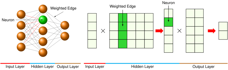](https://mlsysbook.ai/contents/core/dnn_architectures/5aab87381f560ddc7f720233b9e89a654d299fa1.svg "Figure 1: Layered Transformations: Multi-Layer Perceptrons (MLPs) implement dense connectivity through sequential matrix multiplications and non-linear activations, supporting complex feature interactions and hierarchical representations of input data. Each layer transforms the input vector from the previous layer, producing a new vector that serves as input to the subsequent layer, as defined by the equation in the text. Source: [@reagen2017deep].")
Figure 1: **Layered Transformations**: Multi-Layer Perceptrons (MLPs) implement dense connectivity through sequential matrix multiplications and non-linear activations, supporting complex feature interactions and hierarchical representations of input data. Each layer transforms the input vector from the previous layer, producing a new vector that serves as input to the subsequent layer, as defined by the equation in the text. Source: ([Reagen et al. 2017](https://mlsysbook.ai/contents/core/dnn_architectures/dnn_architectures.html#ref-reagen2017deep)
).
Reagen, Brandon, Robert Adolf, Paul Whatmough, Gu-Yeon Wei, and David Brooks. 2017. _Deep Learning for Computer Architects_. Springer International Publishing. [https://doi.org/10.1007/978-3-031-01756-8](https://doi.org/10.1007/978-3-031-01756-8)
.
The dimensions of these operations reveal the computational scale of dense pattern processing:
* Input vector: \\(\\mathbf{h}^{(0)} \\in \\mathbb{R}^{d\_{\\text{in}}}\\) (treated as a row vector in this formulation) represents all potential input features
* Weight matrices: \\(\\mathbf{W}^{(l)} \\in \\mathbb{R}^{d\_{\\text{in}} \\times d\_{\\text{out}}}\\) capture all possible input-output relationships
* Output vector: \\(\\mathbf{h}^{(l)} \\in \\mathbb{R}^{d\_{\\text{out}}}\\) produces transformed representations
**Example:** Concrete Computation Example
Consider a simplified 4-pixel image processed by a 3-neuron hidden layer:
**Input**: \\(\\mathbf{h}^{(0)} = \[0.8, 0.2, 0.9, 0.1\]\\) (4 pixel intensities)
**Weight matrix**: \\(\\mathbf{W}^{(1)} = \\begin{bmatrix} 0.5 & 0.1 & -0.2 \\\\ -0.3 & 0.8 & 0.4 \\\\ 0.2 & -0.4 & 0.6 \\\\ 0.7 & 0.3 & -0.1 \\end{bmatrix}\\) (4×3 matrix)
**Computation**: \\\[\\begin{gather\*} \\mathbf{z}^{(1)} = \\mathbf{h}^{(0)}\\mathbf{W}^{(1)} = \\begin{bmatrix} 0.5×0.8 + (-0.3)×0.2 + 0.2×0.9 + 0.7×0.1 \\\\ 0.1×0.8 + 0.8×0.2 + (-0.4)×0.9 + 0.3×0.1 \\\\ (-0.2)×0.8 + 0.4×0.2 + 0.6×0.9 + (-0.1)×0.1 \\end{bmatrix} \\\\ = \\begin{bmatrix} 0.65 \\\\ -0.17 \\\\ 0.47 \\end{bmatrix} \\end{gather\*}\\\] **After ReLU**: \\(\\mathbf{h}^{(1)} = \[0.65, 0, 0.47\]\\) (negative values zeroed)
Each hidden neuron combines ALL input pixels with different weights, demonstrating unrestricted feature interaction.
The MNIST example demonstrates the practical scale of these operations:
* Each 784-dimensional input (\\(28\\times 28\\) pixels) connects to every neuron in the first hidden layer
* A hidden layer with 100 neurons requires a \\(784\\times 100\\) weight matrix
* Each weight in this matrix represents a learnable relationship between an input pixel and a hidden feature
This algorithmic structure addresses the need for arbitrary feature relationships while creating specific computational patterns that computer systems must accommodate.
#### Architectural Characteristics
This dense connectivity approach creates both advantages and trade-offs. Dense connectivity provides the universal approximation capability established earlier but introduces computational redundancy. While this theoretical power enables MLPs to model any continuous function given sufficient width, this flexibility necessitates numerous parameters to learn relatively simple patterns. The dense connections ensure that every input feature influences every output, yielding maximum expressiveness at the cost of maximum computational expense.
These trade-offs motivate sophisticated optimization techniques that reduce computational demands while preserving model capability. Structured pruning can eliminate 80-90% of connections with minimal accuracy loss, while quantization reduces precision requirements from 32-bit to 8-bit or lower. While **[Chapter 10: Model Optimizations](https://mlsysbook.ai/contents/core/optimizations/optimizations.html#sec-model-optimizations)
** details these compression strategies, the architectural foundations established here determine which optimization approaches prove most effective for dense connectivity patterns, with **[Chapter 11: AI Acceleration](https://mlsysbook.ai/contents/core/hw_acceleration/hw_acceleration.html#sec-ai-acceleration)
** exploring hardware-specific implementations that exploit regular matrix operation structure.
### Computational Mapping
The mathematical representation of dense matrix multiplication maps to specific computational patterns that systems must handle. This mapping progresses from mathematical abstraction to computational reality, as demonstrated in the first implementation shown in [Listing 1](https://mlsysbook.ai/contents/core/dnn_architectures/dnn_architectures.html#lst-mlp_layer_matrix)
.
The function mlp\_layer\_matrix directly mirrors the mathematical equation, employing high-level matrix operations (`matmul`) to express the computation in a single line while abstracting the underlying complexity. This implementation style characterizes deep learning frameworks, where optimized libraries manage the actual computation.
Listing 1: This implementation shows neural networks performing weighted sum and activation functions across layers using matrix operations. The code emphasizes the core computational pattern in multi-layer perceptrons.
def mlp_layer_matrix(X, W, b):
# X: input matrix (batch_size × num_inputs)
# W: weight matrix (num_inputs × num_outputs)
# b: bias vector (num_outputs)
H = activation(matmul(X, W) + b)
# One clean line of math
return H
To understand the system implications of this architecture, we must look “under the hood” of the high-level framework call. The elegant one-line matrix multiplication `output = matmul(X, W)` is, from the hardware’s perspective, a series of nested loops that expose the true computational demands on the system. This translation from logical model to physical execution reveals critical patterns that determine memory access, parallelization strategies, and hardware utilization.
The second implementation, `mlp_layer_compute` (shown in [Listing 2](https://mlsysbook.ai/contents/core/dnn_architectures/dnn_architectures.html#lst-mlp_layer_compute)
), exposes the actual computational pattern through nested loops. This version reveals what really happens when we compute a layer’s output: we process each sample in the batch, computing each output neuron by accumulating weighted contributions from all inputs.
Listing 2: This implementation computes each output neuron by accumulating weighted contributions from all inputs across the batch. The detailed step-by-step process exposes how a single layer in a neural network processes data, emphasizing the role of biases and weighted sums in producing outputs.
def mlp_layer_compute(X, W, b):
# Process each sample in the batch
for batch in range(batch_size):
# Compute each output neuron
for out in range(num_outputs):
# Initialize with bias
Z[batch, out] = b[out]
# Accumulate weighted inputs
for in_ in range(num_inputs):
Z[batch, out] += X[batch, in_] * W[in_, out]
H = activation(Z)
return H
This translation from mathematical abstraction to concrete computation exposes how dense matrix multiplication decomposes into nested loops of simpler operations. The outer loop processes each sample in the batch, while the middle loop computes values for each output neuron. Within the innermost loop, the system performs repeated multiply-accumulate operations[4](https://mlsysbook.ai/contents/core/dnn_architectures/dnn_architectures.html#fn4)
, combining each input with its corresponding weight.
4 **Multiply-Accumulate (MAC)**: The atomic operation in neural networks: multiply two values and add to running sum (result += a × b). Modern accelerators measure performance in MACs/second: NVIDIA A100 achieves 312 trillion MACs/second, while mobile chips achieve 1-10 trillion. Energy cost: ~4.6 picojoules per MAC, plus 640pJ for data movement.
5 **Basic Linear Algebra Subprograms (BLAS)**: Developed in the 1970s as a standard for basic vector and matrix operations, BLAS became the foundation for virtually all scientific computing. Modern implementations like Intel MKL and OpenBLAS can achieve 80-95% of theoretical peak performance on well-optimized workloads, making them necessary for neural network efficiency.
6 **Tensor Cores**: Specialized matrix multiplication units in modern GPUs that perform mixed-precision operations on 4×4 matrices per clock cycle. NVIDIA V100 tensor cores deliver 125 TFLOPS vs 15 TFLOPS from standard cores—a 8× improvement that revolutionized deep learning performance and made large model training feasible.
In the MNIST example, each output neuron requires 784 multiply-accumulate operations and at least 1,568 memory accesses (784 for inputs, 784 for weights). While actual implementations use optimizations through libraries like BLAS[5](https://mlsysbook.ai/contents/core/dnn_architectures/dnn_architectures.html#fn5)
or cuBLAS, these patterns drive key system design decisions. The hardware architectures that accelerate these matrix operations, including GPU tensor cores[6](https://mlsysbook.ai/contents/core/dnn_architectures/dnn_architectures.html#fn6)
and specialized AI accelerators, are covered in **[Chapter 11: AI Acceleration](https://mlsysbook.ai/contents/core/hw_acceleration/hw_acceleration.html#sec-ai-acceleration)
**.
### System Implications
Neural network architectures exhibit distinct system-level characteristics that exhibit three core dimensions for systematic analysis: memory requirements, computation needs, and data movement. This framework enables consistent analysis of how algorithmic patterns influence system design decisions, revealing both commonalities and architecture-specific optimizations. We apply this framework throughout our analysis of each architecture family. These system-level considerations build directly on the foundational concepts of neural network computation patterns, memory systems, and system scaling discussed in **[Chapter 3: Deep Learning Primer](https://mlsysbook.ai/contents/core/dl_primer/dl_primer.html#sec-dl-primer)
**.
#### Memory Requirements
For dense pattern processing, the memory requirements stem from storing and accessing weights, inputs, and intermediate results. In our MNIST example, connecting our 784-dimensional input layer to a hidden layer of 100 neurons requires 78,400 weight parameters. Each forward pass must access all these weights, along with input data and intermediate results. The all-to-all connectivity pattern means there’s no inherent locality in these accesses; every output needs every input and its corresponding weights.
These memory access patterns enable optimization through careful data organization and reuse. Modern processors handle these dense access patterns through specialized approaches: CPUs leverage their cache hierarchy for data reuse, while GPUs employ memory architectures designed for high-bandwidth access to large parameter matrices. Frameworks abstract these optimizations through high-performance matrix operations (as detailed in our earlier analysis).
#### Computation Needs
The core computation revolves around multiply-accumulate operations arranged in nested loops. Each output value requires as many multiply-accumulates as there are inputs. For MNIST, this requires 784 multiply-accumulates per output neuron. With 100 neurons in the hidden layer, 78,400 multiply-accumulates are performed for a single input image. While these operations are simple, their volume and arrangement create specific demands on processing resources.
This computational structure enables specific optimization strategies in modern hardware. The dense matrix multiplication pattern parallelizes across multiple processing units, with each handling different subsets of neurons. Modern hardware accelerators take advantage of this through specialized matrix multiplication units, while software frameworks automatically convert these operations into optimized BLAS (Basic Linear Algebra Subprograms) calls. CPUs and GPUs can both exploit cache locality by carefully tiling the computation to maximize data reuse, though their specific approaches differ based on their architectural strengths.
#### Data Movement
The all-to-all connectivity pattern in MLPs creates significant data movement requirements. Each multiply-accumulate operation needs three pieces of data: an input value, a weight value, and the running sum. For our MNIST example layer, computing a single output value requires moving 784 inputs and 784 weights to wherever the computation occurs. This movement pattern repeats for each of the 100 output neurons, creating large data transfer demands between memory and compute units.
The predictable data movement patterns enable strategic data staging and transfer optimizations. Different architectures address this challenge through various mechanisms; CPUs use prefetching and multi-level caches, while GPUs employ high-bandwidth memory systems and latency hiding through massive threading. Software frameworks orchestrate these data movements through memory management systems that reduce redundant transfers and increase data reuse.
This analysis of MLP computational demands reveals a crucial insight: while dense connectivity provides universal approximation capabilities, it creates significant inefficiencies when data exhibits inherent structure. This mismatch between architectural assumptions and data characteristics motivated the development of specialized approaches that could exploit structural patterns for computational gain.
**Self-Check: Question 1.2**
1. What is a key advantage of using Multi-Layer Perceptrons (MLPs) in machine learning systems?
1. They assume no prior structure in the data, allowing maximum flexibility.
2. They exploit inherent data structures for computational efficiency.
3. They require minimal computational resources compared to specialized architectures.
4. They are inherently more interpretable than other neural network architectures.
2. Explain how the Universal Approximation Theorem influences the architectural choice of using MLPs in machine learning systems.
3. In the context of MNIST digit recognition, why might an MLP be chosen over specialized architectures?
1. MLPs are more efficient in handling high-dimensional data like images.
2. MLPs can exploit the spatial locality of pixel data better than convolutional networks.
3. MLPs provide flexibility to learn arbitrary pixel relationships without assuming spatial structure.
4. MLPs are less computationally intensive than convolutional neural networks.
4. The computational operation that forms the backbone of MLPs and accounts for most of their computation time is known as \_\_\_\_. This operation is crucial for the dense connectivity pattern.
5. How do memory requirements and data movement patterns in MLPs influence system design decisions?
[See Answers →](https://mlsysbook.ai/contents/core/dnn_architectures/dnn_architectures.html#quiz-answer-sec-dnn-architectures-multilayer-perceptrons-dense-pattern-processing-259f)
CNNs: Spatial Pattern Processing
--------------------------------
The computational intensity and parameter requirements of MLPs reveal a mismatch when applied to structured data. Building on the computational complexity considerations outlined in [Section 1.1](https://mlsysbook.ai/contents/core/dnn_architectures/dnn_architectures.html#sec-dnn-architectures-architectural-principles-engineering-tradeoffs-89de)
, this inefficiency motivated the development of architectural patterns that exploit inherent data structure.
Convolutional Neural Networks emerged as the solution to this challenge ([Lecun et al. 1998](https://mlsysbook.ai/contents/core/dnn_architectures/dnn_architectures.html#ref-lecun1998gradient)
; [Krizhevsky, Sutskever, and Hinton 2017](https://mlsysbook.ai/contents/core/dnn_architectures/dnn_architectures.html#ref-krizhevsky2012imagenet)
), embodying a specific inductive bias: they assume spatial locality and translation invariance, where nearby pixels are related and patterns can appear anywhere. This architectural assumption enables two key innovations that enhance efficiency for spatially structured data. Parameter sharing allows the same feature detector to be applied across different spatial positions, reducing parameters from millions to thousands while improving generalization. Local connectivity restricts connections to spatially adjacent regions, reflecting the insight that spatial proximity correlates with feature relevance.
**Definition:** Convolutional Neural Networks
**_Convolutional Neural Networks (CNNs)_** are neural architectures that exploit _spatial structure_ through _local connectivity_ and _parameter sharing_, using _learnable filters_ to build _hierarchical representations_ with substantially fewer parameters than fully-connected networks.
These architectural innovations represent a trade-off in deep learning design: sacrificing the theoretical generality of MLPs for practical efficiency gains when data exhibits known structure. While MLPs treat each input element independently, CNNs exploit spatial relationships to achieve computational savings and improved performance on vision tasks.
### Pattern Processing Needs
Spatial pattern processing addresses scenarios where the relationship between data points depends on their relative positions or proximity. Consider processing a natural image: a pixel’s relationship with its neighbors is important for detecting edges, textures, and shapes. These local patterns then combine hierarchically to form more complex features: edges form shapes, shapes form objects, and objects form scenes.
This hierarchical spatial pattern processing appears across many domains. In computer vision, local pixel patterns form edges and textures that combine into recognizable objects. Speech processing relies on patterns across nearby time segments to identify phonemes and words. Sensor networks analyze correlations between physically proximate sensors to understand environmental patterns. Medical imaging depends on recognizing tissue patterns that indicate biological structures.
Focusing on image processing to illustrate these principles, if we want to detect a cat in an image, certain spatial patterns must be recognized: the triangular shape of ears, the round contours of the face, the texture of fur. Importantly, these patterns maintain their meaning regardless of where they appear in the image. A cat is still a cat whether it appears in the top-left or bottom-right corner. This indicates two key requirements for spatial pattern processing: the ability to detect local patterns and the ability to recognize these patterns regardless of their position[7](https://mlsysbook.ai/contents/core/dnn_architectures/dnn_architectures.html#fn7)
. [Figure 2](https://mlsysbook.ai/contents/core/dnn_architectures/dnn_architectures.html#fig-cnn-spatial-processing)
shows convolutional neural networks achieving this through hierarchical feature extraction, where simple patterns compose into increasingly complex representations at successive layers.
7 **ImageNet Revolution**: AlexNet’s dramatic victory in the 2012 ImageNet challenge ([Krizhevsky, Sutskever, and Hinton 2017](https://mlsysbook.ai/contents/core/dnn_architectures/dnn_architectures.html#ref-krizhevsky2012imagenet)
) (reducing top-5 error from 25.8% to 15.3%) sparked the deep learning renaissance. ImageNet’s 14 million labeled images across 20,000 categories provided the scale needed to train deep CNNs, proving that “big data + big compute + big models” could achieve superhuman performance.
Krizhevsky, Alex, Ilya Sutskever, and Geoffrey E. Hinton. 2017. “ImageNet Classification with Deep Convolutional Neural Networks.” _Communications of the ACM_ 60 (6): 84–90. [https://doi.org/10.1145/3065386](https://doi.org/10.1145/3065386)
.
[](https://mlsysbook.ai/contents/core/dnn_architectures/c8b06853acf5ccdc49c2acfab35b58b178bac9b1.svg "Figure 2: Spatial Feature Extraction: Convolutional neural networks identify patterns independent of their location in an image by applying learnable filters across the input, enabling robust object recognition. These filters detect local features, and their repeated application across the image creates translation invariance, the ability to recognize a pattern regardless of its position.")
Figure 2: **Spatial Feature Extraction**: Convolutional neural networks identify patterns independent of their location in an image by applying learnable filters across the input, enabling robust object recognition. These filters detect local features, and their repeated application across the image creates translation invariance, the ability to recognize a pattern regardless of its position.
This leads us to the convolutional neural network architecture (CNN), pioneered by Yann LeCun[8](https://mlsysbook.ai/contents/core/dnn_architectures/dnn_architectures.html#fn8)
and Y. LeCun et al. ([1989](https://mlsysbook.ai/contents/core/dnn_architectures/dnn_architectures.html#ref-lecun1989backpropagation)
). CNNs achieve this through several key innovations: parameter sharing[9](https://mlsysbook.ai/contents/core/dnn_architectures/dnn_architectures.html#fn9)
, local connectivity, and translation invariance[10](https://mlsysbook.ai/contents/core/dnn_architectures/dnn_architectures.html#fn10)
.
8 **Yann LeCun and CNNs**: LeCun’s 1989 LeNet architecture was inspired by Hubel and Wiesel’s discovery of simple and complex cells in cat visual cortex ([Hubel and Wiesel 1962](https://mlsysbook.ai/contents/core/dnn_architectures/dnn_architectures.html#ref-hubel1962receptive)
). LeNet-5 achieved 99.2% accuracy on MNIST in 1998 (though this was the error rate on a subset, not full MNIST as we know it today) and was deployed by banks to read millions of checks daily, among the first large-scale commercial applications of neural networks.
Hubel, D. H., and T. N. Wiesel. 1962. “Receptive Fields, Binocular Interaction and Functional Architecture in the Cat’s Visual Cortex.” _The Journal of Physiology_ 160 (1): 106–54. [https://doi.org/10.1113/jphysiol.1962.sp006837](https://doi.org/10.1113/jphysiol.1962.sp006837)
.
LeCun, Y., B. Boser, J. S. Denker, D. Henderson, R. E. Howard, W. Hubbard, and L. D. Jackel. 1989. “Backpropagation Applied to Handwritten Zip Code Recognition.” _Neural Computation_ 1 (4): 541–51. [https://doi.org/10.1162/neco.1989.1.4.541](https://doi.org/10.1162/neco.1989.1.4.541)
.
9 **Parameter Sharing**: CNNs reuse the same filter weights across spatial positions, reducing parameters substantially. A CNN processing 224×224 images might use 3×3 filters with only 9 parameters per channel, versus an equivalent MLP requiring 50,176 parameters per neuron, a ~5,575x reduction per neuron enabling practical computer vision.
10 **Translation Invariance**: CNNs detect features regardless of spatial position. A cat’s ear is recognized whether in the top-left or bottom-right corner. This property emerges from convolution’s sliding window design and is important for computer vision, where objects appear at arbitrary locations in images.
### Algorithmic Structure
The core operation in a CNN can be expressed mathematically as:
\\\[ \\mathbf{H}^{(l)}\_{i,j,k} = f\\left(\\sum\_{di}\\sum\_{dj}\\sum\_{c} \\mathbf{W}^{(l)}\_{di,dj,c,k}\\mathbf{H}^{(l-1)}\_{i+di,j+dj,c} + \\mathbf{b}^{(l)}\_k\\right) \\\]
This equation describes how CNNs process spatial data. \\(\\mathbf{H}^{(l)}\_{i,j,k}\\) is the output at spatial position \\((i,j)\\) in channel \\(k\\) of layer \\(l\\). The triple sum iterates over the filter dimensions: \\((di,dj)\\) scans the spatial filter size, and \\(c\\) covers input channels. \\(\\mathbf{W}^{(l)}\_{di,dj,c,k}\\) represents the filter weights, capturing local spatial patterns. Unlike MLPs that connect all inputs to outputs, CNNs only connect local spatial neighborhoods.
Breaking down the notation further, \\((i,j)\\) corresponds to spatial positions, \\(k\\) indexes output channels, \\(c\\) indexes input channels, and \\((di,dj)\\) spans the local receptive field[11](https://mlsysbook.ai/contents/core/dnn_architectures/dnn_architectures.html#fn11)
. Unlike the dense matrix multiplication of MLPs, this operation:
11 **Receptive Field**: The region of the input that influences a particular output neuron. In CNNs, receptive fields grow with depth. A neuron in layer 3 might “see” a 7×7 region even with 3×3 filters, due to stacking. Understanding receptive field size is important for ensuring networks can capture features at the right scale for the task.
* Processes local neighborhoods (typically \\(3\\times 3\\) or \\(5\\times 5\\))
* Reuses the same weights at each spatial position
* Maintains spatial structure in its output
To illustrate this process concretely, consider the MNIST digit classification task with \\(28\\times 28\\) grayscale images. Each convolutional layer applies a set of filters (e.g., \\(3\\times 3\\)) that slide across the image, computing local weighted sums. If we use 32 filters with padding to preserve dimensions, the layer produces a \\(28\\times 28\\times 32\\) output, where each spatial position contains 32 different feature measurements of its local neighborhood. This contrasts sharply with the Multi-Layer Perceptron (MLP) approach, where the entire image is flattened into a 784-dimensional vector before processing.
This algorithmic structure directly implements the requirements for spatial pattern processing, creating distinct computational patterns that influence system design. Unlike MLPs, convolutional networks preserve spatial locality, leveraging the hierarchical feature extraction principles established above. These properties drive architectural optimizations in AI accelerators, where operations such as data reuse, tiling, and parallel filter computation are important for performance.
Mathematical Background
Group theory provides the mathematical framework for understanding symmetries and transformations in data. Translation equivariance means that shifting an input produces a correspondingly shifted output—a key property that enables CNNs to recognize patterns regardless of position.
Group theory provides the framework for understanding CNN effectiveness[12](https://mlsysbook.ai/contents/core/dnn_architectures/dnn_architectures.html#fn12)
, which provides a mathematical framework for understanding symmetries in data. Translation invariance emerges because convolution is equivariant with respect to the translation group—if we shift the input image, the output feature maps shift by the same amount. Mathematically, if \\(T\_v\\) represents translation by vector \\(v\\), then a convolutional layer \\(f\\) satisfies: \\(f(T\_v x) = T\_v f(x)\\). This equivariance property allows CNNs to learn features that generalize across spatial locations.
12 **Group Theory in Neural Networks**: Mathematical framework describing how CNNs preserve spatial relationships. Translation equivariance means shifting an input image shifts the output feature maps by the same amount—a property enabling CNNs to recognize objects regardless of position, foundational to computer vision success.
13 **Inductive Bias**: Prior assumptions built into model architecture about the structure of data. CNNs assume spatial locality and translation invariance, drastically reducing the space of functions they can learn compared to MLPs. This constraint enables better generalization with fewer parameters—a key principle in machine learning architecture design.
14 **Hypothesis Space**: The set of all possible functions a model can represent given its architecture and parameters. MLPs have a larger hypothesis space than CNNs for images, but CNNs’ constrained space contains better solutions for visual tasks, demonstrating that architectural constraints often improve rather than limit performance. Recent work has extended these principles to other symmetry groups, developing Group-Equivariant CNNs that handle rotations and reflections ([Cohen and Welling 2016](https://mlsysbook.ai/contents/core/dnn_architectures/dnn_architectures.html#ref-cohen2016group)
).
Cohen, Taco, and Max Welling. 2016. “Group Equivariant Convolutional Networks.” _International Conference on Machine Learning_, 2990–99.
The choice of convolution reflects deeper principles about inductive bias[13](https://mlsysbook.ai/contents/core/dnn_architectures/dnn_architectures.html#fn13)
in neural architecture design. By restricting connectivity to local neighborhoods and sharing parameters across spatial positions, CNNs encode prior knowledge about the structure of visual data: that important features are local and translation-invariant. This architectural constraint reduces the hypothesis space[14](https://mlsysbook.ai/contents/core/dnn_architectures/dnn_architectures.html#fn14)
that the network must search, enabling more efficient learning from limited data compared to fully connected networks.
CNNs naturally implement hierarchical representation learning through their layered structure. Early layers detect low-level features like edges and textures with small receptive fields, while deeper layers combine these into increasingly complex patterns with larger receptive fields. This hierarchical organization mirrors the structure of the visual cortex and enables CNNs to build compositional representations: complex objects are represented as compositions of simpler parts. The mathematical foundation for this emerges from the fact that stacking convolutional layers creates a tree-like dependency structure, where each deep neuron depends on an exponentially large set of input pixels, enabling efficient representation of hierarchical patterns.
#### Architectural Characteristics
Parameter sharing dramatically reduces complexity compared to MLPs by reusing the same filters across spatial locations. This sharing embodies the assumption that useful features (such as edges or textures) can appear anywhere in an image, making the same feature detector valuable across all spatial positions.
The architectural efficiency of CNNs enables further optimization through specialized techniques. Depthwise separable convolutions decompose standard convolutions into depthwise and pointwise operations, reducing computation by 8-9× for typical mobile deployments. Channel pruning eliminates entire feature maps based on importance metrics, achieving 40-50% FLOPs reduction with <1% accuracy loss. These optimization strategies build on spatial locality principles, with **[Chapter 10: Model Optimizations](https://mlsysbook.ai/contents/core/optimizations/optimizations.html#sec-model-optimizations)
** exploring hardware-specific implementations and **[Chapter 11: AI Acceleration](https://mlsysbook.ai/contents/core/hw_acceleration/hw_acceleration.html#sec-ai-acceleration)
** detailing how modern processors exploit convolution’s inherent data reuse patterns.
As illustrated in [Figure 3](https://mlsysbook.ai/contents/core/dnn_architectures/dnn_architectures.html#fig-cnn)
, convolution operations involve sliding a small filter over the input image to generate a feature map[15](https://mlsysbook.ai/contents/core/dnn_architectures/dnn_architectures.html#fn15)
. This process captures local structures while maintaining translation invariance. For an interactive visual exploration of convolutional networks, the [CNN Explainer](https://poloclub.github.io/cnn-explainer/)
project provides an insightful demonstration of how these networks are constructed.
15 **Feature Map**: The output of applying a convolutional filter to an input, representing detected features at different spatial locations. A 64-filter layer produces 64 feature maps, each highlighting different patterns like edges, textures, or shapes. Feature maps become more abstract (detecting objects, faces) in deeper layers compared to early layers (detecting edges, colors).
[](https://mlsysbook.ai/contents/core/dnn_architectures/fc7cbac26cbac9fcfc0d4c00b2bae655b6fafb65.svg "Figure 3: The convolution operation processes input data through localized feature extraction using filters that slide across the image to identify patterns regardless of their position.")
Figure 3: The convolution operation processes input data through localized feature extraction using filters that slide across the image to identify patterns regardless of their position.
### Computational Mapping
Convolution operations create computational patterns different from MLP dense matrix multiplication. This translation from mathematical operations to implementation details reveals distinct computational characteristics.
The first implementation, `conv_layer_spatial` (shown in [Listing 3](https://mlsysbook.ai/contents/core/dnn_architectures/dnn_architectures.html#lst-conv_layer_spatial)
), uses high-level convolution operations to express the computation concisely. This is typical in deep learning frameworks, where optimized libraries handle the underlying complexity.
Listing 3: This hierarchical approach processes input data through feature extraction using a convolution operation that combines a kernel and bias before applying an activation function.
def conv_layer_spatial(input, kernel, bias):
output = convolution(input, kernel) + bias
return activation(output)
The bridge between the logical model and physical execution becomes critical for understanding CNN system requirements. While the high-level convolution operation appears as a simple sliding window computation, the hardware must orchestrate complex data movement patterns and exploit spatial locality for efficiency.
The second implementation, conv\_layer\_compute (see [Listing 4](https://mlsysbook.ai/contents/core/dnn_architectures/dnn_architectures.html#lst-conv_layer_compute)
), reveals the actual computational pattern: nested loops that process each spatial position, applying the same filter weights to local regions of the input. These seven nested loops expose the true nature of convolution’s computational structure and the optimization opportunities it creates.
Listing 4: **Nested Loops**: Convolutional layers process input through multiple nested loops that handle batched images, spatial dimensions, output channels, kernel windows, and input features, revealing the detailed computational structure of convolution operations.
def conv_layer_compute(input, kernel, bias):
# Loop 1: Process each image in batch
for image in range(batch_size):
# Loop 2&3: Move across image spatially
for y in range(height):
for x in range(width):
# Loop 4: Compute each output feature
for out_channel in range(num_output_channels):
result = bias[out_channel]
# Loop 5&6: Move across kernel window
for ky in range(kernel_height):
for kx in range(kernel_width):
# Loop 7: Process each input feature
for in_channel in range(
num_input_channels
):
# Get input value from correct window position
in_y = y + ky
in_x = x + kx
# Perform multiply-accumulate operation
result += (
input[\
image, in_y, in_x, in_channel\
]
* kernel[\
ky,\
kx,\
in_channel,\
out_channel,\
]
)
# Store result for this output position
output[image, y, x, out_channel] = result
The seven nested loops reveal different aspects of the computation:
* Outer loops (1-3) manage position: which image and where in the image
* Middle loop (4) handles output features: computing different learned patterns
* Inner loops (5-7) perform the actual convolution: sliding the kernel window
Examining this process in detail, the outer two loops (`for y` and `for x`) traverse each spatial position in the output feature map (for the MNIST example, this traverses all \\(28\\times 28\\) positions). At each position, values are computed for each output channel (`for k` loop), representing different learned features or patterns—the 32 different feature detectors.
The inner three loops implement the actual convolution operation at each position. For each output value, we process a local \\(3\\times 3\\) region of the input (the `dy` and `dx` loops) across all input channels (`for c` loop). This creates a sliding window effect, where the same \\(3\\times 3\\) filter moves across the image, performing multiply-accumulates between the filter weights and the local input values. Unlike the MLP’s global connectivity, this local processing pattern means each output value depends only on a small neighborhood of the input.
For our MNIST example with \\(3\\times 3\\) filters and 32 output channels, each output position requires only 9 multiply-accumulate operations per input channel, compared to the 784 operations needed in our MLP layer. This operation must be repeated for every spatial position \\((28\\times 28)\\) and every output channel (32).
While using fewer operations per output, the spatial structure creates different patterns of memory access and computation that systems must handle. These patterns influence system design, creating both challenges and opportunities for optimization.
### System Implications
CNNs exhibit distinctive system-level patterns that differ significantly from MLP dense connectivity across all three analysis dimensions.
#### Memory Requirements
For convolutional layers, memory requirements center around two key components: filter weights and feature maps. Unlike MLPs that require storing full connection matrices, CNNs use small, reusable filters. For a typical CNN processing 224×224 ImageNet images, a convolutional layer with 64 filters of size \\(3\\times 3\\) requires storing only 576 weight parameters \\((3\\times 3\\times 64)\\), dramatically less than the millions of weights needed for equivalent fully-connected processing. The system must store feature maps for all spatial positions, creating a different memory demand. A 224×224 input with 64 output channels requires storing 3.2 million activation values (224×224×64).
These memory access patterns suggest opportunities for optimization through weight reuse and careful feature map management. Processors optimize these spatial patterns by caching filter weights for reuse across positions while streaming feature map data. Frameworks implement spatial optimizations through specialized memory layouts that enable filter reuse and spatial locality in feature map access. CPUs and GPUs approach this differently. CPUs use their cache hierarchy to keep frequently used filters resident, while GPUs employ specialized memory architectures designed for the spatial access patterns of image processing. The detailed architecture design principles for these specialized processors are covered in **[Chapter 11: AI Acceleration](https://mlsysbook.ai/contents/core/hw_acceleration/hw_acceleration.html#sec-ai-acceleration)
**.
#### Computation Needs
The core computation in CNNs involves repeatedly applying small filters across spatial positions. Each output value requires a local multiply-accumulate operation over the filter region. For ImageNet processing with \\(3\\times 3\\) filters and 64 output channels, computing one spatial position involves 576 multiply-accumulates \\((3\\times 3\\times 64)\\), and this must be repeated for all 50,176 spatial positions (224×224). While each individual computation involves fewer operations than an MLP layer, the total computational load remains large due to spatial repetition.
This computational pattern presents different optimization opportunities than MLPs. The regular, repeated nature of convolution operations enables efficient hardware utilization through structured parallelism. Modern processors exploit this pattern in various ways. CPUs leverage SIMD instructions[16](https://mlsysbook.ai/contents/core/dnn_architectures/dnn_architectures.html#fn16)
to process multiple filter positions simultaneously, while GPUs parallelize computation across spatial positions and channels. The model optimization techniques that further reduce these computational demands, including specialized convolution optimizations and sparsity patterns, are detailed in **[Chapter 10: Model Optimizations](https://mlsysbook.ai/contents/core/optimizations/optimizations.html#sec-model-optimizations)
**.
16 **SIMD (Single Instruction, Multiple Data)**: CPU instructions that perform the same operation on multiple data elements simultaneously. Modern x86 processors support AVX-512, enabling 16 single-precision operations per instruction, a 16x speedup over scalar code. SIMD is important for efficient neural network inference on CPUs, especially for edge deployment. Deep learning frameworks further optimize this through specialized convolution algorithms that transform the computation to better match hardware capabilities.
#### Data Movement
The sliding window pattern of convolutions creates a distinctive data movement profile. Unlike MLPs where each weight is used once per forward pass, CNN filter weights are reused many times as the filter slides across spatial positions. For ImageNet processing, each \\(3\\times 3\\) filter weight is reused 50,176 times (once for each position in the 224×224 feature map). This creates a different challenge: the system must stream input features through the computation unit while keeping filter weights stable.
The predictable spatial access pattern enables strategic data movement optimizations. Different architectures handle this movement pattern through specialized mechanisms. CPUs maintain frequently used filter weights in cache while streaming through input features. GPUs employ memory architectures optimized for spatial locality and provide hardware support for efficient sliding window operations. Deep learning frameworks orchestrate these movements by organizing computations to maximize filter weight reuse and minimize redundant feature map accesses.
**Self-Check: Question 1.3**
1. Which architectural feature of CNNs allows them to efficiently process spatially structured data?
1. Global connectivity
2. Parameter sharing
3. Both B and D
4. Local connectivity
2. Explain how parameter sharing in CNNs contributes to computational efficiency compared to MLPs.
3. In CNNs, the ability to detect features regardless of their spatial position is known as \_\_\_\_.
4. Order the following CNN operations as they occur in a typical layer: (1) Apply filter, (2) Activation function, (3) Bias addition.
5. In a production system, how might the architectural characteristics of CNNs influence hardware design decisions?
[See Answers →](https://mlsysbook.ai/contents/core/dnn_architectures/dnn_architectures.html#quiz-answer-sec-dnn-architectures-cnns-spatial-pattern-processing-f8ff)
RNNs: Sequential Pattern Processing
-----------------------------------
Convolutional Neural Networks achieved efficiency gains by exploiting spatial locality, yet their architectural assumptions fail when patterns depend on temporal order rather than spatial proximity. While CNNs excel at recognizing "what" is present in data through shared feature detectors, they cannot capture "when" events occur or how they relate across time. This limitation manifests in domains such as natural language processing, where word meaning depends on sentential context, and time-series analysis, where future values depend on historical patterns.
Sequential data presents a challenge distinct from spatial processing: patterns can span arbitrary temporal distances, rendering fixed-size kernels ineffective. While spatial convolution leverages the principle that nearby pixels are typically related, temporal relationships operate differently. Important connections may span hundreds or thousands of time steps with no correlation to proximity. Traditional feedforward architectures, including CNNs, process each input independently and cannot maintain the temporal context necessary for these long-range dependencies.
Recurrent Neural Networks address this architectural limitation ([Elman 1990](https://mlsysbook.ai/contents/core/dnn_architectures/dnn_architectures.html#ref-elman1990finding)
; [Hochreiter and Schmidhuber 1997](https://mlsysbook.ai/contents/core/dnn_architectures/dnn_architectures.html#ref-hochreiter1997long)
) by embodying a temporal inductive bias: they assume sequential dependence, where the order of information matters and the past influences the present. This architectural assumption guides the introduction of memory as a component of the computational model. Rather than processing inputs in isolation, RNNs maintain an internal state that propagates information from previous time steps, enabling the network to condition its current output on historical context. This architecture embodies another trade-off: while CNNs sacrifice theoretical generality for spatial efficiency, RNNs introduce computational dependencies that challenge parallel execution in exchange for temporal processing capabilities.
**Definition:** Recurrent Neural Networks
**_Recurrent Neural Networks (RNNs)_** are sequential neural architectures that maintain _internal memory state_ across time steps through _recurrent connections_, enabling _variable-length sequence processing_ at the cost of _sequential computation_ that prevents parallelization.
Coverage Note
This section covers of RNNs, emphasizing their core contributions to sequential processing and the architectural principles that influenced modern attention mechanisms. While RNNs introduced critical concepts—memory states, temporal dependencies, and sequential computation—contemporary practice increasingly favors attention-based architectures for sequence modeling. We focus on foundational principles rather than extensive implementation variants, dedicating significant depth to the attention mechanisms and Transformers ([Section 1.5](https://mlsysbook.ai/contents/core/dnn_architectures/dnn_architectures.html#sec-dnn-architectures-attention-mechanisms-dynamic-pattern-processing-566d)
) that have largely superseded RNNs in production systems while building directly on the insights gained from recurrent architectures.
### Pattern Processing Needs
Sequential pattern processing addresses scenarios where current input interpretation depends on preceding information. In natural language processing, word meaning often depends heavily on previous words in the sentence. Context determines interpretation, as evidenced by the varying meanings of words based on surrounding terms. Similarly, in speech recognition, phoneme interpretation depends on surrounding sounds, while financial forecasting requires understanding historical data patterns.
The challenge in sequential processing lies in maintaining and updating relevant context over time. Human text comprehension does not restart with each word; rather, a running understanding evolves as new information is processed. Similarly, time-series data processing encounters patterns spanning different timescales, from immediate dependencies to long-term trends. This necessitates an architecture capable of both maintaining state over time and updating it based on new inputs.
These requirements translate into specific architectural demands: the system must maintain internal state to capture temporal context, update this state based on new inputs, and learn which historical information is relevant for current predictions. Unlike MLPs and CNNs, which process fixed-size inputs, sequential processing must accommodate variable-length sequences while maintaining computational efficiency. These requirements culminate in the recurrent neural network (RNN) architecture.
### Algorithmic Structure
RNNs address sequential processing through recurrent connections, distinguishing them from MLPs and CNNs. Rather than merely mapping inputs to outputs, RNNs maintain an internal state updated at each time step, creating a memory mechanism that propagates information forward in time. This temporal dependency modeling capability was first explored by Elman ([1990](https://mlsysbook.ai/contents/core/dnn_architectures/dnn_architectures.html#ref-elman1990finding)
), who demonstrated RNN capacity to identify structure in time-dependent data. Basic RNNs suffer from the vanishing gradient problem[17](https://mlsysbook.ai/contents/core/dnn_architectures/dnn_architectures.html#fn17)
, constraining their ability to learn long-term dependencies.
17 **Vanishing Gradient Problem**: During backpropagation through time, gradients shrink exponentially as they propagate backward through RNN layers. When recurrent weights have magnitude < 1, gradients multiply by values < 1 at each time step, vanishing after 5-10 steps and preventing learning of long-term dependencies—a key limitation solved by LSTMs and attention mechanisms.
The core operation in a basic RNN can be expressed mathematically as: \\\[ \\mathbf{h}\_t = f(\\mathbf{W}\_{hh}\\mathbf{h}\_{t-1} + \\mathbf{W}\_{xh}\\mathbf{x}\_t + \\mathbf{b}\_h) \\\] where \\(\\mathbf{h}\_t\\) denotes the hidden state at time \\(t\\), \\(\\mathbf{x}\_t\\) denotes the input at time \\(t\\), \\(\\mathbf{W}\_{hh}\\) contains the recurrent weights, and \\(\\mathbf{W}\_{xh}\\) contains the input weights, as illustrated in the unfolded network structure in [Figure 4](https://mlsysbook.ai/contents/core/dnn_architectures/dnn_architectures.html#fig-rnn)
.
In word sequence processing, each word may be represented as a 100-dimensional vector (\\(\\mathbf{x}\_t\\)), with a hidden state of 128 dimensions (\\(\\mathbf{h}\_t\\)). At each time step, the network combines the current input with its previous state to update its sequential understanding, establishing a memory mechanism capable of capturing patterns across time steps.
This recurrent structure fulfills sequential processing requirements through connections that maintain internal state and propagate information forward in time. Rather than processing all inputs independently, RNNs process sequential data by iteratively updating a hidden state based on the current input and the previous hidden state, as depicted in [Figure 4](https://mlsysbook.ai/contents/core/dnn_architectures/dnn_architectures.html#fig-rnn)
. This architecture suits tasks including language modeling, speech recognition, and time-series forecasting.
RNNs implement a recursive algorithm where each time step’s function call depends on the result of the previous call. Analogous to recursive functions that maintain state through the call stack, RNNs maintain state through their hidden vectors. The mathematical formula \\(\\mathbf{h}\_t = f(\\mathbf{h}\_{t-1}, \\mathbf{x}\_t)\\) directly parallels recursive function definitions where `f(n) = g(f(n-1), input(n))`. This correspondence explains RNN capacity to handle variable-length sequences: just as recursive algorithms process lists of arbitrary length by applying the same function recursively, RNNs process sequences of any length by applying the same recurrent computation.
#### Efficiency and Optimization
Sequential processing creates computational bottlenecks but enables unique efficiency characteristics for memory usage. RNNs achieve constant memory overhead for hidden state storage regardless of sequence length, making them extremely memory-efficient for long sequences. While Transformers require O(n²) memory for sequence length n, RNNs maintain fixed memory usage, enabling processing of sequences thousands of steps long on modest hardware.
Structured pruning of hidden-to-hidden connections can achieve 10x speedup while maintaining sequence modeling capability. The recurrent weight matrix \\(W\_{hh}\\) typically dominates parameter count for large hidden states, but magnitude-based pruning reveals that 70-80% of these connections contribute minimally to temporal dependencies. Block-structured pruning maintains computational efficiency while enabling significant model compression.
Sequential operations accumulate quantization errors, requiring careful quantization point placement and gradient scaling for stable low-precision training. Unlike feedforward networks where quantization errors remain localized, RNN errors propagate through time, making INT8 quantization more challenging. Per-timestep quantization schemes and careful handling of hidden state precision are required for maintaining accuracy in quantized RNN deployments.
[](https://mlsysbook.ai/contents/core/dnn_architectures/00d28078c95f0324945a05b54b6eed89ff2acb28.svg "Figure 4: Recurrent Neural Network Unfolding: Rnns process sequential data by maintaining a hidden state that incorporates information from previous time steps through this diagram. the unfolded structure explicitly represents the temporal dependencies modeled by the recurrent weights, enabling the network to learn patterns across variable-length sequences.")
Figure 4: **Recurrent Neural Network Unfolding**: Rnns process sequential data by maintaining a hidden state that incorporates information from previous time steps through this diagram. the unfolded structure explicitly represents the temporal dependencies modeled by the recurrent weights, enabling the network to learn patterns across variable-length sequences.
### Computational Mapping
RNN sequential processing creates computational patterns different from both MLPs and CNNs, extending the architectural diversity discussed in [Section 1.1](https://mlsysbook.ai/contents/core/dnn_architectures/dnn_architectures.html#sec-dnn-architectures-architectural-principles-engineering-tradeoffs-89de)
. This implementation approach shows temporal dependencies translating into specific computational requirements.
As shown in [Listing 5](https://mlsysbook.ai/contents/core/dnn_architectures/dnn_architectures.html#lst-rnn_layer_step)
, the `rnn_layer_step` function shows the operation using high-level matrix operations found in deep learning frameworks. It handles a single time step, taking the current input `x_t` and previous hidden state `h_prev`, along with two weight matrices: `W_hh` for hidden-to-hidden connections and `W_xh` for input-to-hidden connections. Through matrix multiplication operations (`matmul`), it merges the previous state and current input to generate the next hidden state.
Listing 5: **RNN Layer Step**: Neural networks process sequential data through transformations that integrate current inputs and past states.
def rnn_layer_step(x_t, h_prev, W_hh, W_xh, b):
# x_t: input at time t (batch_size × input_dim)
# h_prev: previous hidden state (batch_size × hidden_dim)
# W_hh: recurrent weights (hidden_dim × hidden_dim)
# W_xh: input weights (input_dim × hidden_dim)
h_t = activation(matmul(h_prev, W_hh) + matmul(x_t, W_xh) + b)
return h_t
Understanding RNN system implications requires examining how the elegant mathematical abstraction translates into hardware execution patterns. The simple recurrence relation `h_t = tanh(W_hh h_{t-1} + W_xh x_t + b)` conceals a computational structure that creates unique challenges: sequential dependencies that prevent parallelization, memory access patterns that differ from feedforward networks, and state management requirements that affect system design.
The detailed implementation ([Listing 6](https://mlsysbook.ai/contents/core/dnn_architectures/dnn_architectures.html#lst-rnn_layer_compute)
) reveals the computational reality beneath the mathematical abstraction. The nested loop structure exposes how sequential processing creates both limitations and opportunities in system optimization.
Listing 6: **Recurrent Layer Computation**: Computes the hidden state at each time step through sequential transformations involving previous states and current inputs.
def rnn_layer_compute(x_t, h_prev, W_hh, W_xh, b):
# Initialize next hidden state
h_t = np.zeros_like(h_prev)
# Loop 1: Process each sequence in the batch
for batch in range(batch_size):
# Loop 2: Compute recurrent contribution
# (h_prev × W_hh)
for i in range(hidden_dim):
for j in range(hidden_dim):
h_t[batch, i] += h_prev[batch, j] * W_hh[j, i]
# Loop 3: Compute input contribution (x_t × W_xh)
for i in range(hidden_dim):
for j in range(input_dim):
h_t[batch, i] += x_t[batch, j] * W_xh[j, i]
# Loop 4: Add bias and apply activation
for i in range(hidden_dim):
h_t[batch, i] = activation(h_t[batch, i] + b[i])
return h_t
The nested loops in `rnn_layer_compute` expose the core computational pattern of RNNs (see [Listing 6](https://mlsysbook.ai/contents/core/dnn_architectures/dnn_architectures.html#lst-rnn_layer_compute)
). Loop 1 processes each sequence in the batch independently, allowing for batch-level parallelism. Within each batch item, Loop 2 computes how the previous hidden state influences the next state through the recurrent weights `W_hh`. Loop 3 then incorporates new information from the current input through the input weights `W_xh`. Finally, Loop 4 adds biases and applies the activation function to produce the new hidden state.
For a sequence processing task with input dimension 100 and hidden state dimension 128, each time step requires two matrix multiplications: one \\(128\\times 128\\) for the recurrent connection and one \\(100\\times 128\\) for the input projection. While individual time steps can process in parallel across batch elements, the time steps themselves must process sequentially. This creates a unique computational pattern that systems must handle.
### System Implications
Following the analytical framework established for MLPs, RNNs exhibit distinctive patterns in memory requirements, computation needs, and data movement that differ significantly from both dense and spatial processing architectures.
#### Memory Requirements
RNNs require storing two sets of weights (input-to-hidden and hidden-to-hidden) along with the hidden state. For the example with input dimension 100 and hidden state dimension 128, this requires storing 12,800 weights for input projection \\((100\\times 128)\\) and 16,384 weights for recurrent connections \\((128\\times 128)\\). Unlike CNNs where weights are reused across spatial positions, RNN weights are reused across time steps. The system must maintain the hidden state, which constitutes a key factor in memory usage and access patterns.
These memory access patterns create a different profile from MLPs and CNNs. Processors optimize sequential patterns by maintaining weight matrices in cache while streaming through temporal elements. Frameworks optimize temporal processing by batching sequences and managing hidden state storage between time steps. CPUs and GPUs approach this through different strategies; CPUs leverage their cache hierarchy for weight reuse; meanwhile, GPUs use specialized memory architectures designed for maintaining state across sequential operations. The specialized hardware optimizations for sequential processing, including memory banking and pipeline architectures, are detailed in **[Chapter 11: AI Acceleration](https://mlsysbook.ai/contents/core/hw_acceleration/hw_acceleration.html#sec-ai-acceleration)
**.
#### Computation Needs
The core computation in RNNs involves repeatedly applying weight matrices across time steps. For each time step, we perform two matrix multiplications: one with the input weights and one with the recurrent weights. In our example, processing a single time step requires 12,800 multiply-accumulates for the input projection \\((100\\times 128)\\) and 16,384 multiply-accumulates for the recurrent connection \\((128\\times 128)\\).
This computational pattern differs from both MLPs and CNNs in a key way: while we can parallelize across batch elements, we cannot parallelize across time steps due to the sequential dependency. Each time step must wait for the previous step’s hidden state before it can begin computation. This creates a tension between the inherent sequential nature of the algorithm and the desire for parallel execution in modern hardware.
Processors address sequential constraints through specialized approaches. CPUs pipeline operations within time steps while maintaining temporal ordering. GPUs batch multiple sequences together to maintain high throughput despite sequential dependencies. Software frameworks optimize this further by techniques like sequence packing and unrolling computations across multiple time steps when possible, enabling more efficient utilization of parallel processing resources while respecting the sequential constraints inherent in recurrent architectures.
#### Data Movement
The sequential processing in RNNs creates a distinctive data movement pattern that differs from both MLPs and CNNs. While MLPs need each weight only once per forward pass and CNNs reuse weights across spatial positions, RNNs reuse their weights across time steps while requiring careful management of the hidden state data flow.
For our example with a 128-dimensional hidden state, each time step must: load the previous hidden state (128 values), access both weight matrices (29,184 total weights from both input and recurrent connections), and store the new hidden state (128 values). This pattern repeats for every element in the sequence. Unlike CNNs where we can predict and prefetch data based on spatial patterns, RNN data movement is driven by temporal dependencies.
Different architectures handle this sequential data movement through specialized mechanisms. CPUs maintain weight matrices in cache while streaming through sequence elements and managing hidden state updates. GPUs employ memory architectures optimized for maintaining state information across sequential operations while processing multiple sequences in parallel. Deep learning frameworks orchestrate these movements by managing data transfers between time steps and optimizing batch operations.
While RNNs established concepts for sequential processing, their architectural constraints create bottlenecks: sequential dependencies prevent parallelization across time steps, fixed-capacity hidden states create information bottlenecks for long sequences, and temporal proximity assumptions break down when important relationships span distant positions. These limitations motivated the development of attention mechanisms, which eliminate sequential processing constraints through dynamic, content-dependent connectivity. The following section examines how attention mechanisms address each of these RNN limitations while introducing new computational challenges. This extensive treatment reflects attention mechanisms’ dominance in modern ML systems and their fundamental reimagining of sequential pattern processing.
**Self-Check: Question 1.4**
1. What is the primary advantage of RNNs over CNNs when processing sequential data?
1. RNNs maintain an internal state to capture temporal dependencies.
2. RNNs can process data in parallel across time steps.
3. RNNs are more efficient in terms of memory usage than CNNs.
4. RNNs use fixed-size kernels to capture patterns.
2. Explain how RNNs handle long-term dependencies in sequential data and discuss one limitation related to this capability.
3. The phenomenon where gradients shrink exponentially as they propagate backward through RNN layers is known as the \_\_\_\_. This limits the ability of RNNs to learn long-term dependencies.
4. In a production system, how might the sequential processing nature of RNNs influence hardware design and optimization strategies?
[See Answers →](https://mlsysbook.ai/contents/core/dnn_architectures/dnn_architectures.html#quiz-answer-sec-dnn-architectures-rnns-sequential-pattern-processing-ea14)
Attention Mechanisms: Dynamic Pattern Processing
------------------------------------------------
Recurrent Neural Networks successfully introduced memory to handle sequential dependencies, but their fixed sequential processing creates limitations. RNNs process information in temporal order, making it difficult to capture relationships between distant elements and impossible to parallelize computation across sequence positions. More critically, RNNs assume that temporal proximity correlates with importance—that nearby words or time steps are more relevant than distant ones. This assumption breaks down in many real-world scenarios.
Consider the sentence "The cat, which was sitting by the window overlooking the garden, was sleeping." Here, "cat" and "sleeping" are separated by multiple intervening words, yet they form the core subject-predicate relationship. RNN architectures would process all the intervening elements sequentially, potentially losing this crucial connection in their fixed-capacity hidden state. This limitation revealed the need for architectures that could identify and weight relationships based on content rather than position.
Attention mechanisms emerged as the solution to this architectural constraint ([Bahdanau, Cho, and Bengio 2014](https://mlsysbook.ai/contents/core/dnn_architectures/dnn_architectures.html#ref-bahdanau2014neural)
) by introducing dynamic connectivity patterns that adapt based on input content. Rather than processing elements in predetermined order with fixed relationships, attention mechanisms compute the relevance between all pairs of elements and weight their interactions accordingly. This represents a shift from structural constraints to learned, data-dependent processing patterns.
**Definition:** Attention Mechanisms
**_Attention Mechanisms_** are neural components that compute _content-dependent relationships_ between sequence elements through _query-key-value operations_, enabling _selective focus_ on relevant information and _long-range dependencies_ without positional constraints.
While attention mechanisms were initially used as components within recurrent architectures, the Transformer architecture ([Vaswani et al. 2017](https://mlsysbook.ai/contents/core/dnn_architectures/dnn_architectures.html#ref-vaswani2017attention)
) demonstrated that attention alone could entirely replace sequential processing, creating a new architectural paradigm.
**Definition:** Transformers
**_Transformers_** are neural architectures based entirely on _attention mechanisms_, using _multi-head self-attention_ and _position encodings_ to process sequences in _parallel_ rather than sequentially, enabling efficient training and inference at scale.
### Pattern Processing Needs
Dynamic pattern processing addresses scenarios where relationships between elements are not fixed by architecture but instead emerge from content. Language translation exemplifies this challenge: when translating “the bank by the river,” understanding “bank” requires attending to “river,” but in “the bank approved the loan,” the important relationship is with “approved” and “loan.” Unlike RNNs that process information sequentially or CNNs that use fixed spatial patterns, an architecture is required that can dynamically determine which relationships matter.
Expanding beyond language, this requirement for dynamic processing appears across many domains. In protein structure prediction, interactions between amino acids depend on their chemical properties and spatial arrangements. In graph analysis, node relationships vary based on graph structure and node features. In document analysis, connections between different sections depend on semantic content rather than just proximity.
Synthesizing these requirements, dynamic processing demands specific capabilities from our processing architecture. The system must compute relationships between all pairs of elements, weigh these relationships based on content, and use these weights to selectively combine information. Unlike previous architectures with fixed connectivity patterns, dynamic processing requires the flexibility to modify its computation graph based on the input itself. These capabilities naturally lead us to the attention mechanism, which serves as the foundation for the Transformer architecture examined in detail in the following sections. [Figure 5](https://mlsysbook.ai/contents/core/dnn_architectures/dnn_architectures.html#fig-transformer-attention-visualized)
shows attention enabling this dynamic information flow.
[](https://mlsysbook.ai/contents/core/dnn_architectures/0ac6a22c6278235896e8ca59ca4a0d5274e79296.svg "Figure 5: Attention Weights: Transformer attention mechanisms dynamically assess relationships between subwords, assigning higher weights to more relevant connections within a sequence and enabling the model to focus on key information. These learned weights, visualized as connection strengths, reveal how the model attends to different parts of the input when processing language.")
Figure 5: **Attention Weights**: Transformer attention mechanisms dynamically assess relationships between subwords, assigning higher weights to more relevant connections within a sequence and enabling the model to focus on key information. These learned weights, visualized as connection strengths, reveal how the model attends to different parts of the input when processing language.
### Basic Attention Mechanism
Attention mechanisms represent a shift from fixed architectural connections to dynamic, content-based interactions between sequence elements. This section explores the mathematical foundations of attention, examining how query-key-value operations enable flexible pattern processing. We analyze the computational requirements, memory access patterns, and system implications that make attention both powerful and computationally demanding.
#### Algorithmic Structure
Attention mechanisms form the foundation of dynamic pattern processing by computing weighted connections between elements based on their content ([Bahdanau, Cho, and Bengio 2014](https://mlsysbook.ai/contents/core/dnn_architectures/dnn_architectures.html#ref-bahdanau2014neural)
). This approach processes relationships that are not fixed by architecture but instead emerge from the data itself. At the core of an attention mechanism lies an operation that can be expressed mathematically as:
\\\[ \\text{Attention}(\\mathbf{Q}, \\mathbf{K}, \\mathbf{V}) = \\text{softmax} \\left(\\frac{\\mathbf{Q}\\mathbf{K}^T}{\\sqrt{d\_k}}\\right)\\mathbf{V} \\\]
This equation shows scaled dot-product attention. \\(\\mathbf{Q}\\) (queries) and \\(\\mathbf{K}\\) (keys) are matrix-multiplied to compute similarity scores, divided by \\(\\sqrt{d\_k}\\) (key dimension) for numerical stability, then normalized with softmax[18](https://mlsysbook.ai/contents/core/dnn_architectures/dnn_architectures.html#fn18)
to get attention weights. These weights are applied to \\(\\mathbf{V}\\) (values) to produce the output. The result is a weighted combination where each position receives information from all relevant positions based on content similarity.
18 **Softmax Function**: Converts a vector of real numbers into a probability distribution where all values sum to 1. Defined as \\(\\text{softmax}(x\_i) = \\frac{e^{x\_i}}{\\sum\_j e^{x\_j}}\\), softmax amplifies differences between inputs (larger values get disproportionately higher probabilities) while ensuring valid attention weights for combining information sources.
19 **Query-Key-Value Attention**: Inspired by information retrieval systems where queries search through keys to retrieve values. In neural attention, queries and keys compute similarity scores (like a search engine matching queries to documents), while values contain the actual information to retrieve—a design that enables flexible, content-based information access.
In this equation, \\(\\mathbf{Q}\\) (queries), \\(\\mathbf{K}\\) (keys), and \\(\\mathbf{V}\\) (values)[19](https://mlsysbook.ai/contents/core/dnn_architectures/dnn_architectures.html#fn19)
represent learned projections of the input. For a sequence of length \\(N\\) with dimension \\(d\\), this operation creates an \\(N\\times N\\) attention matrix, determining how each position should attend to all others.
The attention operation involves several key steps. First, it computes query, key, and value projections for each position in the sequence. Next, it generates an \\(N\\times N\\) attention matrix through query-key interactions. These steps are illustrated in [Figure 6](https://mlsysbook.ai/contents/core/dnn_architectures/dnn_architectures.html#fig-attention)
. Finally, it uses these attention weights to combine value vectors, producing the output.
[](https://mlsysbook.ai/contents/core/dnn_architectures/0f88d09d466d8e0373bbe53f1318aa4872ac0a9f.svg "Figure 6: Query-Key-Value Interaction: Transformer attention mechanisms dynamically weigh input sequence elements by computing relationships between queries, keys, and values, enabling the model to focus on relevant information. these projections facilitate the creation of an attention matrix that determines the contribution of each value vector to the final output, effectively capturing contextual dependencies within the sequence. Source: transformer explainer.")
Figure 6: **Query-Key-Value Interaction**: Transformer attention mechanisms dynamically weigh input sequence elements by computing relationships between queries, keys, and values, enabling the model to focus on relevant information. these projections facilitate the creation of an attention matrix that determines the contribution of each value vector to the final output, effectively capturing contextual dependencies within the sequence. Source: [transformer explainer](https://poloclub.github.io/transformer-explainer/)
.
The key is that, unlike the fixed weight matrices found in previous architectures, as shown in [Figure 7](https://mlsysbook.ai/contents/core/dnn_architectures/dnn_architectures.html#fig-attention-weightcalc)
, these attention weights are computed dynamically for each input. This allows the model to adapt its processing based on the dynamic content at hand.
[](https://mlsysbook.ai/contents/core/dnn_architectures/ac01feea1f3247fae0b2bc06f5f4339a5e6cacec.svg "Figure 7: Dynamic Attention Weights: Transformer models calculate attention weights dynamically based on the relationships between query, key, and value vectors, allowing the model to focus on relevant parts of the input sequence for each processing step. this contrasts with fixed-weight architectures and enables adaptive pattern processing for handling variable-length inputs and complex dependencies. Source: transformer explainer.")
Figure 7: **Dynamic Attention Weights**: Transformer models calculate attention weights dynamically based on the relationships between query, key, and value vectors, allowing the model to focus on relevant parts of the input sequence for each processing step. this contrasts with fixed-weight architectures and enables adaptive pattern processing for handling variable-length inputs and complex dependencies. Source: [transformer explainer](https://poloclub.github.io/transformer-explainer/)
.
#### Computational Mapping
Attention mechanisms create computational patterns that differ significantly from previous architectures. The implementation approach shown in [Listing 7](https://mlsysbook.ai/contents/core/dnn_architectures/dnn_architectures.html#lst-attention_layer_compute)
shows dynamic connectivity translating into specific computational requirements.
Listing 7: **Attention Mechanism**: Transformer models compute attention through query-key-value interactions, enabling dynamic focus across input sequences for improved language understanding.
def attention_layer_matrix(Q, K, V):
# Q, K, V: (batch_size × seq_len × d_model)
scores = matmul(Q, K.transpose(-2, -1)) / sqrt(
d_k
) # Compute attention scores
weights = softmax(scores) # Normalize scores
output = matmul(weights, V) # Combine values
return output
# Core computational pattern
def attention_layer_compute(Q, K, V):
# Initialize outputs
scores = np.zeros((batch_size, seq_len, seq_len))
outputs = np.zeros_like(V)
# Loop 1: Process each sequence in batch
for b in range(batch_size):
# Loop 2: Compute attention for each query position
for i in range(seq_len):
# Loop 3: Compare with each key position
for j in range(seq_len):
# Compute attention score
for d in range(d_model):
scores[b, i, j] += Q[b, i, d] * K[b, j, d]
scores[b, i, j] /= sqrt(d_k)
# Apply softmax to scores
for i in range(seq_len):
scores[b, i] = softmax(scores[b, i])
# Loop 4: Combine values using attention weights
for i in range(seq_len):
for j in range(seq_len):
for d in range(d_model):
outputs[b, i, d] += scores[b, i, j] * V[b, j, d]
return outputs
The translation from attention’s mathematical elegance to hardware execution reveals the computational price of dynamic connectivity. While the attention equation `Attention(Q,K,V) = softmax(QK^T/√d_k)V` appears as a straightforward matrix operation, the physical implementation requires orchestrating quadratic numbers of pairwise computations that create different system demands than previous architectures.
The nested loops in `attention_layer_compute` expose attention’s true computational signature (see [Listing 7](https://mlsysbook.ai/contents/core/dnn_architectures/dnn_architectures.html#lst-attention_layer_compute)
). The first loop processes each sequence in the batch independently. The second and third loops compute attention scores between all pairs of positions, creating the quadratic computation pattern that makes attention both powerful and computationally demanding. The fourth loop uses these attention weights to combine values from all positions, completing the dynamic connectivity pattern that defines attention mechanisms.
#### System Implications
Attention mechanisms exhibit distinctive system-level patterns that differ from previous architectures through their dynamic connectivity requirements.
##### Memory Requirements
In terms of memory requirements, attention mechanisms necessitate storage for attention weights, key-query-value projections, and intermediate feature representations. For a sequence length \\(N\\) and dimension d, each attention layer must store an \\(N\\times N\\) attention weight matrix for each sequence in the batch, three sets of projection matrices for queries, keys, and values (each sized \\(d\\times d\\)), and input and output feature maps of size \\(N\\times d\\). The dynamic generation of attention weights for every input creates a memory access pattern where intermediate attention weights become a significant factor in memory usage.
##### Computation Needs
Computation needs in attention mechanisms center around two main phases: generating attention weights and applying them to values. For each attention layer, the system performs many multiply-accumulate operations across multiple computational stages. The query-key interactions alone require \\(N\\times N\\times d\\) multiply-accumulates, with an equal number needed for applying attention weights to values. Additional computations are required for the projection matrices and softmax operations. This computational pattern differs from previous architectures due to its quadratic scaling with sequence length and the need to perform fresh computations for each input.
##### Data Movement
Data movement in attention mechanisms presents unique challenges. Each attention operation involves projecting and moving query, key, and value vectors for each position, storing and accessing the full attention weight matrix, and coordinating the movement of value vectors during the weighted combination phase. This creates a data movement pattern where intermediate attention weights become a major factor in system bandwidth requirements. Unlike the more predictable access patterns of CNNs or the sequential access of RNNs, attention operations require frequent movement of dynamically computed weights across the memory hierarchy.
These distinctive characteristics of attention mechanisms in terms of memory, computation, and data movement have significant implications for system design and optimization, setting the stage for the development of more advanced architectures like Transformers.
### Transformers: Attention-Only Architecture
While attention mechanisms introduced the concept of dynamic pattern processing, they were initially applied as additions to existing architectures, particularly RNNs for sequence-to-sequence tasks. This hybrid approach still suffered from the fundamental limitations of recurrent architectures: sequential processing constraints that prevented efficient parallelization and difficulties with very long sequences. The breakthrough insight was recognizing that attention mechanisms alone could replace both convolutional and recurrent processing entirely.
Transformers, introduced in the landmark "Attention is All You Need" paper[20](https://mlsysbook.ai/contents/core/dnn_architectures/dnn_architectures.html#fn20)
by Vaswani et al. ([2017](https://mlsysbook.ai/contents/core/dnn_architectures/dnn_architectures.html#ref-vaswani2017attention)
), embody a revolutionary inductive bias: **they assume no prior structure but allow the model to learn all pairwise relationships dynamically based on content**. This architectural assumption represents the culmination of the architectural evolution detailed in [Section 1.1](https://mlsysbook.ai/contents/core/dnn_architectures/dnn_architectures.html#sec-dnn-architectures-architectural-principles-engineering-tradeoffs-89de)
by eliminating all structural constraints in favor of pure content-dependent processing. Rather than adding attention to RNNs, Transformers built the entire architecture around attention mechanisms, introducing self-attention as the primary computational pattern. This architectural decision traded the parameter efficiency of CNNs and the sequential coherence of RNNs for maximum flexibility and parallelizability.
20 **“Attention is All You Need”**: This 2017 paper by Google researchers eliminated recurrence entirely, showing that attention mechanisms alone could achieve state-of-the-art results. The title itself became a rallying cry, and within 5 years, transformer-based models achieved breakthrough performance in language (GPT, BERT), vision (ViT), and beyond ([Radford et al. 2018](https://mlsysbook.ai/contents/core/dnn_architectures/dnn_architectures.html#ref-radford2018improving)
; [Devlin et al. 2018](https://mlsysbook.ai/contents/core/dnn_architectures/dnn_architectures.html#ref-devlin2018bert)
; [Dosovitskiy et al. 2021](https://mlsysbook.ai/contents/core/dnn_architectures/dnn_architectures.html#ref-dosovitskiy2021image)
). This paper marked a historical turning point in deep learning, demonstrating that the sequential processing that defined RNNs and LSTMs was no longer necessary; attention mechanisms could capture both short and long-range dependencies through parallel computation. While the basic attention mechanism allows for content-based weighting of information from a source sequence, Transformers extend this idea by applying attention within a single sequence, enabling each element to attend to all other elements including itself.
Radford, Alec, Karthik Narasimhan, Tim Salimans, and Ilya Sutskever. 2018. “Improving Language Understanding by Generative Pre-Training.”
Devlin, Jacob, Ming-Wei Chang, Kenton Lee, and Kristina Toutanova. 2018. “BERT: Pre-Training of Deep Bidirectional Transformers for Language Understanding.” _arXiv Preprint arXiv:1810.04805_, October. [http://arxiv.org/abs/1810.04805v2](http://arxiv.org/abs/1810.04805v2)
.
Dosovitskiy, Alexey, Lucas Beyer, Alexander Kolesnikov, Dirk Weissenborn, Xiaohua Zhai, Thomas Unterthiner, Mostafa Dehghani, et al. 2021. “An Image Is Worth 16x16 Words: Transformers for Image Recognition at Scale.” _International Conference on Learning Representations_.
Vaswani, Ashish, Noam Shazeer, Niki Parmar, Jakob Uszkoreit, Llion Jones, Aidan N Gomez, Kaiser, and Illia Polosukhin. 2017. “Attention Is All You Need.” _Advances in Neural Information Processing Systems_ 30.
This represents the final step in our architectural journey: from MLPs that connected everything to everything, to CNNs that connected locally, to RNNs that connected sequentially, to Transformers that connect dynamically based on learned content relationships. Each evolution sacrificed constraints for capabilities, with Transformers achieving maximum expressivity at the computational cost established in [Section 1.1](https://mlsysbook.ai/contents/core/dnn_architectures/dnn_architectures.html#sec-dnn-architectures-architectural-principles-engineering-tradeoffs-89de)
.
#### Algorithmic Structure
The key innovation in Transformers lies in their use of self-attention layers. In the self-attention mechanism used by Transformers, the Query, Key, and Value vectors are all derived from the same input sequence. This is the key distinction from earlier attention mechanisms where the query might come from a decoder while the keys and values came from an encoder. By making all components self-referential, self-attention allows the model to weigh the importance of different positions within the same sequence when encoding each position. For instance, in processing the sentence “The animal didn’t cross the street because it was too wide,” self-attention allows the model to link “it” with “street,” capturing long-range dependencies that are challenging for traditional sequential models.
The self-attention mechanism can be expressed mathematically in a form similar to the basic attention mechanism: \\\[ \\text{SelfAttention}(\\mathbf{X}) = \\text{softmax} \\left(\\frac{\\mathbf{XW\_Q}(\\mathbf{XW\_K})^T}{\\sqrt{d\_k}}\\right)\\mathbf{XW\_V} \\\]
Here, \\(\\mathbf{X}\\) is the input sequence, and \\(\\mathbf{W\_Q}\\), \\(\\mathbf{W\_K}\\), and \\(\\mathbf{W\_V}\\) are learned weight matrices for queries, keys, and values respectively. This formulation highlights how self-attention derives all its components from the same input, creating a dynamic, content-dependent processing pattern.
Building on this foundation, Transformers employ multi-head attention, which extends the self-attention mechanism by running multiple attention functions in parallel. Each “head” involves a separate set of query/key/value projections that can focus on different aspects of the input, allowing the model to jointly attend to information from different representation subspaces. This multi-head structure provides the model with a richer representational capability, enabling it to capture various types of relationships within the data simultaneously.
The mathematical formulation for multi-head attention is: \\\[ \\text{MultiHead}(\\mathbf{Q}, \\mathbf{K}, \\mathbf{V}) = \\text{Concat}(\\text{head}\_1, \\ldots, \\text{head}\_h)\\mathbf{W}^O \\\] where each attention head is computed as: \\\[ \\text{head}\_i = \\text{Attention}(\\mathbf{Q}\\mathbf{W}\_i^Q, \\mathbf{K}\\mathbf{W}\_i^K, \\mathbf{V}\\mathbf{W}\_i^V) \\\]
A critical component in both self-attention and multi-head attention is the scaling factor \\(\\sqrt{d\_k}\\), which serves an important mathematical purpose. This factor prevents the dot products from growing too large, which would push the softmax function into regions with extremely small gradients. For queries and keys of dimension \\(d\_k\\), their dot product has variance \\(d\_k\\), so dividing by \\(\\sqrt{d\_k}\\) normalizes the variance to 1, maintaining stable gradients and enabling effective learning.[21](https://mlsysbook.ai/contents/core/dnn_architectures/dnn_architectures.html#fn21)
21 **Attention Scaling**: Without the \\(\\sqrt{d\_k}\\) scaling factor, large dot products would cause the softmax to saturate, producing gradients close to zero and hindering learning. This mathematical insight enables stable optimization of large Transformer models.
Beyond the mathematical mechanics, attention mechanisms can be understood conceptually as implementing a form of content-addressable memory system. Like hash tables that retrieve values based on key matching, attention computes similarity between a query and all available keys, then retrieves a weighted combination of corresponding values. The dot product similarity `Q·K` functions like a hash function that measures how well each key matches the query. The softmax normalization ensures the weights sum to 1, implementing a probabilistic retrieval mechanism. This connection explains why attention proves effective for tasks requiring flexible information retrieval—it provides a differentiable approximation to database lookup operations.
From an information-theoretic perspective, attention mechanisms implement optimal information aggregation under uncertainty. The attention weights represent uncertainty about which parts of the input contain relevant information for the current processing step. The softmax operation implements a maximum entropy principle: among all possible ways to distribute attention across input positions, softmax selects the distribution with maximum entropy subject to the constraint that similarity scores determine relative importance ([Cover and Thomas 2001](https://mlsysbook.ai/contents/core/dnn_architectures/dnn_architectures.html#ref-cover2006elements)
).
Cover, Thomas M., and Joy A. Thomas. 2001. _Elements of Information Theory_. 2nd ed. Wiley. [https://doi.org/10.1002/0471200611](https://doi.org/10.1002/0471200611)
.
#### Efficiency and Optimization
Attention mechanisms are highly redundant, with many heads learning similar patterns. Head pruning and low-rank attention factorization can reduce computation by 50-80% with careful implementation. Analysis of large Transformer models reveals that most attention heads fall into a few common patterns (positional, syntactic, semantic), suggesting that explicit architectural specialization could replace learned redundancy.
Attention operations are particularly sensitive to quantization due to the softmax operation and the quadratic number of attention scores. Separate quantization schemes for Q, K, V projections and careful handling of softmax operations are required for stable quantization. Post-training INT8 quantization typically achieves 2-3% accuracy loss, while INT4 quantization requires more sophisticated quantization-aware training approaches.
The quadratic scaling with sequence length creates efficiency limitations. Sparse attention patterns (such as local windows, strided patterns, or learned sparsity) can reduce complexity from O(n²) to O(n log n) or O(n) while maintaining most modeling capability. Linear attention approximations trade some expressive power for linear scaling, enabling processing of much longer sequences on limited hardware.
This information-theoretic interpretation reveals why attention is so effective for selective processing. The mechanism automatically balances two competing objectives: focusing on the most relevant information (minimizing entropy) while maintaining sufficient breadth to avoid missing important details (maximizing entropy). The attention pattern emerges as the optimal trade-off between these objectives, explaining why transformers can effectively handle long sequences and complex dependencies.
Self-attention learns dynamic activation patterns across the input sequence. Unlike CNNs which apply fixed filters or RNNs which use fixed recurrence patterns, attention learns which elements should activate together based on their content. This creates a form of adaptive connectivity where the effective network topology changes for each input. Recent research has shown that attention heads in trained models often specialize in detecting specific linguistic or semantic patterns ([Clark et al. 2019](https://mlsysbook.ai/contents/core/dnn_architectures/dnn_architectures.html#ref-clark2019what)
), suggesting that the mechanism naturally discovers interpretable structural regularities in data.
Clark, Kevin, Urvashi Khandelwal, Omer Levy, and Christopher D. Manning. 2019. “What Does BERT Look at? An Analysis of BERT’s Attention.” In _Proceedings of the 2019 ACL Workshop BlackboxNLP: Analyzing and Interpreting Neural Networks for NLP_, 276–86. Association for Computational Linguistics. [https://doi.org/10.18653/v1/w19-4828](https://doi.org/10.18653/v1/w19-4828)
.
The Transformer architecture leverages this self-attention mechanism within a broader structure that typically includes feed-forward layers, layer normalization, and residual connections (see [Figure 8](https://mlsysbook.ai/contents/core/dnn_architectures/dnn_architectures.html#fig-transformer)
). This combination allows Transformers to process input sequences in parallel, capturing complex dependencies without the need for sequential computation. As a result, Transformers have demonstrated significant effectiveness across a wide range of tasks, from natural language processing to computer vision, transforming deep learning architectures across domains.
[](https://mlsysbook.ai/contents/core/dnn_architectures/aa3aa170a3acdaf91ddfd26c9ea74821e1dd5a86.svg "Figure 8: Attention Head: Neural networks compute attention through query-key-value interactions, enabling dynamic focus across subwords for improved sentence understanding. Source: Attention Is All You Need.")
Figure 8: **Attention Head**: Neural networks compute attention through query-key-value interactions, enabling dynamic focus across subwords for improved sentence understanding. Source: Attention Is All You Need.
#### Computational Mapping
While Transformer self-attention builds upon the basic attention mechanism, it introduces distinct computational patterns that set it apart. To understand these patterns, we must examine the typical implementation of self-attention in Transformers (see [Listing 8](https://mlsysbook.ai/contents/core/dnn_architectures/dnn_architectures.html#lst-self_attention_layer)
):
Listing 8: **Self-Attention Mechanism**: Transformer models compute attention through query-key-value interactions, enabling dynamic focus across input sequences for improved language understanding.
def self_attention_layer(X, W_Q, W_K, W_V, d_k):
# X: input tensor (batch_size × seq_len × d_model)
# W_Q, W_K, W_V: weight matrices (d_model × d_k)
Q = matmul(X, W_Q)
K = matmul(X, W_K)
V = matmul(X, W_V)
scores = matmul(Q, K.transpose(-2, -1)) / sqrt(d_k)
attention_weights = softmax(scores, dim=-1)
output = matmul(attention_weights, V)
return output
def multi_head_attention(X, W_Q, W_K, W_V, W_O, num_heads, d_k):
outputs = []
for i in range(num_heads):
head_output = self_attention_layer(
X, W_Q[i], W_K[i], W_V[i], d_k
)
outputs.append(head_output)
concat_output = torch.cat(outputs, dim=-1)
final_output = matmul(concat_output, W_O)
return final_output
#### System Implications
This implementation reveals key computational characteristics that apply to basic attention mechanisms, with Transformer self-attention representing a specific case. First, self-attention enables parallel processing across all positions in the sequence. This is evident in the matrix multiplications that compute `Q`, `K`, and `V` simultaneously for all positions. Unlike recurrent architectures that process inputs sequentially, this parallel nature allows for more efficient computation, especially on modern hardware designed for parallel operations.
Second, the attention score computation results in a matrix of size `(seq_len × seq_len)`, leading to quadratic complexity with respect to sequence length. This quadratic relationship becomes a significant computational bottleneck when processing long sequences, a challenge that has spurred research into more efficient attention mechanisms.
Third, the multi-head attention mechanism effectively runs multiple self-attention operations in parallel, each with its own set of learned projections. While this increases the computational load linearly with the number of heads, it allows the model to capture different types of relationships within the same input, enhancing the model’s representational power.
Fourth, the core computations in self-attention are dominated by large matrix multiplications. For a sequence of length \\(N\\) and embedding dimension \\(d\\), the main operations involve matrices of sizes \\((N\\times d)\\), \\((d\\times d)\\), and \\((N\\times N)\\). These intensive matrix operations are well-suited for acceleration on specialized hardware like GPUs, but they also contribute significantly to the overall computational cost of the model.
Finally, self-attention generates memory-intensive intermediate results. The attention weights matrix \\((N\\times N)\\) and the intermediate results for each attention head create large memory requirements, especially for long sequences. This can pose challenges for deployment on memory-constrained devices and necessitates careful memory management in implementations.
These computational patterns create a unique profile for Transformer self-attention, distinct from previous architectures. The parallel nature of the computations makes Transformers well-suited for modern parallel processing hardware, but the quadratic complexity with sequence length poses challenges for processing long sequences. As a result, much research has focused on developing optimization techniques, such as sparse attention patterns or low-rank approximations, to address these challenges. Each of these optimizations presents its own trade-offs between computational efficiency and model expressiveness, a balance that must be carefully considered in practical applications.
This examination of four distinct architectural families reveals both their individual characteristics and their collective evolution. Rather than viewing these architectures in isolation, a deeper understanding emerges when we consider how they relate to each other and build upon shared foundations.
**Self-Check: Question 1.5**
1. Which of the following best describes the primary advantage of attention mechanisms over RNNs?
1. Attention mechanisms process sequences in parallel, capturing long-range dependencies more effectively.
2. Attention mechanisms use fixed spatial patterns to process data.
3. Attention mechanisms rely on sequential processing to capture temporal dependencies.
4. Attention mechanisms are less computationally demanding than RNNs.
2. Explain how attention mechanisms dynamically determine which relationships in input data are important.
3. In attention mechanisms, the operation that normalizes similarity scores to create a probability distribution is called the \_\_\_\_.
4. In a production system, what are the computational trade-offs of implementing attention mechanisms compared to RNNs?
[See Answers →](https://mlsysbook.ai/contents/core/dnn_architectures/dnn_architectures.html#quiz-answer-sec-dnn-architectures-attention-mechanisms-dynamic-pattern-processing-566d)
Architectural Building Blocks
-----------------------------
Having examined four major architectural families—MLPs, CNNs, RNNs, and Transformers—each with distinct computational characteristics and system implications, a unifying perspective emerges. Deep learning architectures, while presented as distinct approaches in previous sections, are better understood as compositions of building blocks that evolved over time. Like complex LEGO structures built from basic bricks, modern neural networks combine and iterate on core computational patterns that emerged through decades of research ([Yann LeCun, Bengio, and Hinton 2015](https://mlsysbook.ai/contents/core/dnn_architectures/dnn_architectures.html#ref-lecun2015deep)
). Each architectural innovation introduced new building blocks while discovering novel applications of existing ones.
LeCun, Yann, Yoshua Bengio, and Geoffrey Hinton. 2015. “Deep Learning.” _Nature_ 521 (7553): 436–44. [https://doi.org/10.1038/nature14539](https://doi.org/10.1038/nature14539)
.
Rosenblatt, F. 1958. “The Perceptron: A Probabilistic Model for Information Storage and Organization in the Brain.” _Psychological Review_ 65 (6): 386–408. [https://doi.org/10.1037/h0042519](https://doi.org/10.1037/h0042519)
.
Rumelhart, David E., Geoffrey E. Hinton, and Ronald J. Williams. 1986. “Learning Representations by Back-Propagating Errors.” _Nature_ 323 (6088): 533–36. [https://doi.org/10.1038/323533a0](https://doi.org/10.1038/323533a0)
.
These building blocks and their evolution illuminate modern architectural design. The simple perceptron ([Rosenblatt 1958](https://mlsysbook.ai/contents/core/dnn_architectures/dnn_architectures.html#ref-rosenblatt1958perceptron)
) evolved into multi-layer networks ([Rumelhart, Hinton, and Williams 1986](https://mlsysbook.ai/contents/core/dnn_architectures/dnn_architectures.html#ref-rumelhart1986learning)
), which subsequently spawned specialized patterns for spatial and sequential processing. Each advancement preserved useful elements from predecessors while introducing new computational primitives. Contemporary architectures, such as Transformers, represent carefully engineered combinations of these building blocks.
This progression reveals both the evolution of neural networks and the discovery and refinement of core computational patterns that remain relevant. Building on the architectural progression outlined in [Section 1.1](https://mlsysbook.ai/contents/core/dnn_architectures/dnn_architectures.html#sec-dnn-architectures-architectural-principles-engineering-tradeoffs-89de)
, each new architecture introduces distinct computational demands and system-level challenges.
[Table 1](https://mlsysbook.ai/contents/core/dnn_architectures/dnn_architectures.html#tbl-dl-evolution)
summarizes this evolution, highlighting the key primitives and system focus for each era of deep learning development. This table captures the major shifts in deep learning architecture design and corresponding changes in system-level considerations. The progression spans from early dense matrix operations optimized for CPUs, through convolutions leveraging GPU acceleration and sequential operations necessitating sophisticated memory hierarchies, to the current era of attention mechanisms requiring flexible accelerators and high-bandwidth memory.
Table 1: **Deep Learning Evolution**: Neural network architectures have progressed from simple, fully connected layers to complex models leveraging specialized hardware and addressing sequential data dependencies. This table maps architectural eras to key computational primitives and corresponding system-level optimizations, revealing a historical trend toward increased parallelism and memory bandwidth requirements.
| | | | |
| --- | --- | --- | --- |
| **Early NN** | MLP | Dense Matrix Ops | CPU optimization |
| **CNN Revolution** | CNN | Convolutions | GPU acceleration |
| **Sequence Modeling** | RNN | Sequential Ops | Memory hierarchies |
| **Attention Era** | Transformer | Attention, Dynamic Compute | Flexible accelerators, High-bandwidth memory |
Examination of these building blocks shows primitives evolving and combining to create increasingly powerful neural network architectures.
### Evolution from Perceptron to Multi-Layer Networks
While we examined MLPs in [Section 1.2](https://mlsysbook.ai/contents/core/dnn_architectures/dnn_architectures.html#sec-dnn-architectures-multilayer-perceptrons-dense-pattern-processing-259f)
as a mechanism for dense pattern processing, here we focus on how they established building blocks that appear throughout deep learning. The evolution from perceptron to MLP introduced several key concepts: the power of layer stacking, the importance of non-linear transformations, and the basic feedforward computation pattern.
The introduction of hidden layers between input and output created a template for feature transformation that appears in virtually every modern architecture. Even in sophisticated networks like Transformers, we find MLP-style feedforward layers performing feature processing. The concept of transforming data through successive non-linear layers has become a paradigm that transcends specific architecture types.
Most significantly, the development of MLPs established the backpropagation algorithm[22](https://mlsysbook.ai/contents/core/dnn_architectures/dnn_architectures.html#fn22)
, which to this day remains the cornerstone of neural network optimization. This key contribution has enabled the development of deep architectures and influenced how later architectures would be designed to maintain gradient flow.
22 **Backpropagation Algorithm**: While the chain rule was known since the 1600s, Rumelhart, Hinton, and Williams (1986) showed how to efficiently apply it to train multi-layer networks. This “learning by error propagation” algorithm made deep networks practical and remains virtually unchanged in modern systems—a testament to its importance.
These building blocks, layered feature transformation, non-linear activation, and gradient-based learning, set the foundation for more specialized architectures. Subsequent innovations often focused on structuring these basic components in new ways rather than replacing them entirely.
### Evolution from Dense to Spatial Processing
The development of CNNs marked an architectural innovation, specifically the realization that we could specialize the dense connectivity of MLPs for spatial patterns. While retaining the core concept of layer-wise processing, CNNs introduced several building blocks that would influence all future architectures.
The first key innovation was the concept of parameter sharing. Unlike MLPs where each connection had its own weight, CNNs showed how the same parameters could be reused across different parts of the input. This not only made the networks more efficient but introduced the powerful idea that architectural structure could encode useful priors about the data ([Lecun et al. 1998](https://mlsysbook.ai/contents/core/dnn_architectures/dnn_architectures.html#ref-lecun1998gradient)
).
Lecun, Y., L. Bottou, Y. Bengio, and P. Haffner. 1998. “Gradient-Based Learning Applied to Document Recognition.” _Proceedings of the IEEE_ 86 (11): 2278–2324. [https://doi.org/10.1109/5.726791](https://doi.org/10.1109/5.726791)
.
23 **ResNet Revolution**: ResNet (2016) solved the “degradation problem” where deeper networks performed worse than shallow ones. The key insight: adding identity shortcuts (\\(\\mathcal{F}(\\mathbf{x}) + \\mathbf{x}\\)) let networks learn residual mappings instead of full transformations, enabling training of 1000+ layer networks and winning ImageNet 2015.
He, Kaiming, Xiangyu Zhang, Shaoqing Ren, and Jian Sun. 2016. “Deep Residual Learning for Image Recognition.” In _2016 IEEE Conference on Computer Vision and Pattern Recognition (CVPR)_, 770–78. IEEE. [https://doi.org/10.1109/cvpr.2016.90](https://doi.org/10.1109/cvpr.2016.90)
.
Perhaps even more influential was the introduction of skip connections through ResNets[23](https://mlsysbook.ai/contents/core/dnn_architectures/dnn_architectures.html#fn23)
([He et al. 2016](https://mlsysbook.ai/contents/core/dnn_architectures/dnn_architectures.html#ref-he2016deep)
). Originally they were designed to help train very deep CNNs, skip connections have become a building block that appears in virtually every modern architecture. They showed how direct paths through the network could help gradient flow and information propagation, a concept now central to Transformer designs.
CNNs also introduced batch normalization, a technique for stabilizing neural network optimization by normalizing intermediate features ([Ioffe and Szegedy 2015](https://mlsysbook.ai/contents/core/dnn_architectures/dnn_architectures.html#ref-ioffe2015batch)
). This concept of feature normalization, while originating in CNNs, evolved into layer normalization and is now a key component in modern architectures.
Ioffe, Sergey, and Christian Szegedy. 2015. “Batch Normalization: Accelerating Deep Network Training by Reducing Internal Covariate Shift.” _International Conference on Machine Learning_, 448–56.
These innovations, such as parameter sharing, skip connections, and normalization, transcended their origins in spatial processing to become essential building blocks in the deep learning toolkit.
### Evolution of Sequence Processing
While CNNs specialized MLPs for spatial patterns, sequence models adapted neural networks for temporal dependencies. RNNs introduced the concept of maintaining and updating state, a building block that influenced how networks could process sequential information, ([Elman 1990](https://mlsysbook.ai/contents/core/dnn_architectures/dnn_architectures.html#ref-elman1990finding)
).
Elman, Jeffrey L. 1990. “Finding Structure in Time.” _Cognitive Science_ 14 (2): 179–211. [https://doi.org/10.1207/s15516709cog1402\\\_1](https://doi.org/10.1207/s15516709cog1402/_1)
.
24 **LSTM Origins**: Sepp Hochreiter and Jürgen Schmidhuber invented LSTMs in 1997 to solve the “vanishing gradient problem” that plagued RNNs. Their gating mechanism was inspired by biological neurons’ ability to selectively retain information—a breakthrough that enabled sequence modeling and facilitated modern language models.
25 **Gated Recurrent Unit (GRU)**: Simplified version of LSTM introduced by Cho et al. (2014) with only 2 gates instead of 3, reducing parameters by ~25% while maintaining similar performance. GRUs became popular for their computational efficiency and easier training, proving that architectural simplification can sometimes improve rather than hurt performance.
Hochreiter, Sepp, and Jürgen Schmidhuber. 1997. “Long Short-Term Memory.” _Neural Computation_ 9 (8): 1735–80. [https://doi.org/10.1162/neco.1997.9.8.1735](https://doi.org/10.1162/neco.1997.9.8.1735)
.
Cho, Kyunghyun, Bart van Merrienboer, Dzmitry Bahdanau, and Yoshua Bengio. 2014. “On the Properties of Neural Machine Translation: Encoder-Decoder Approaches.” In _Eighth Workshop on Syntax, Semantics and Structure in Statistical Translation (SSST-8)_, 103–11. Association for Computational Linguistics.
The development of LSTMs[24](https://mlsysbook.ai/contents/core/dnn_architectures/dnn_architectures.html#fn24)
and GRUs[25](https://mlsysbook.ai/contents/core/dnn_architectures/dnn_architectures.html#fn25)
brought sophisticated gating mechanisms to neural networks ([Hochreiter and Schmidhuber 1997](https://mlsysbook.ai/contents/core/dnn_architectures/dnn_architectures.html#ref-hochreiter1997long)
; [Cho et al. 2014](https://mlsysbook.ai/contents/core/dnn_architectures/dnn_architectures.html#ref-cho2014properties)
). These gates, themselves small MLPs, showed how simple feedforward computations could be composed to control information flow. This concept of using neural networks to modulate other neural networks became a recurring pattern in architecture design.
Perhaps most significantly, sequence models demonstrated the power of adaptive computation paths. Unlike the fixed patterns of MLPs and CNNs, RNNs showed how networks could process variable-length inputs by reusing weights over time. This insight, that architectural patterns could adapt to input structure, laid groundwork for more flexible architectures.
Sequence models also popularized the concept of attention through encoder-decoder architectures ([Bahdanau, Cho, and Bengio 2014](https://mlsysbook.ai/contents/core/dnn_architectures/dnn_architectures.html#ref-bahdanau2014neural)
). Initially introduced as an improvement to machine translation, attention mechanisms showed how networks could learn to dynamically focus on relevant information. This building block would later become the foundation of Transformer architectures.
Bahdanau, Dzmitry, Kyunghyun Cho, and Yoshua Bengio. 2014. “Neural Machine Translation by Jointly Learning to Align and Translate.” _arXiv Preprint arXiv:1409.0473_, September. [http://arxiv.org/abs/1409.0473v7](http://arxiv.org/abs/1409.0473v7)
.
### Modern Architectures: Synthesis and Unification
Modern architectures, particularly Transformers, represent a sophisticated synthesis of these fundamental building blocks. Rather than introducing entirely new patterns, they innovate through strategic combination and refinement of existing components. The Transformer architecture exemplifies this approach: at its core, MLP-style feedforward networks process features between attention layers. The attention mechanism itself builds on sequence model concepts while eliminating recurrent connections, instead employing position embeddings inspired by CNN intuitions. The architecture extensively utilizes skip connections (see [Figure 9](https://mlsysbook.ai/contents/core/dnn_architectures/dnn_architectures.html#fig-example-skip-connection)
), inherited from ResNets, while layer normalization, evolved from CNN batch normalization, stabilizes optimization ([Ba, Kiros, and Hinton 2016](https://mlsysbook.ai/contents/core/dnn_architectures/dnn_architectures.html#ref-ba2016layer)
).
Ba, Jimmy Lei, Jamie Ryan Kiros, and Geoffrey E. Hinton. 2016. “Layer Normalization.” _arXiv Preprint arXiv:1607.06450_, July. [http://arxiv.org/abs/1607.06450v1](http://arxiv.org/abs/1607.06450v1)
.
[](https://mlsysbook.ai/contents/core/dnn_architectures/72dd6cccbe43b09e773930fb403ff04d18ab90f1.svg "Figure 9: Residual Connection: Skip connections add the input of a layer to its output, enabling gradients to flow directly through the network and mitigating the vanishing gradient problem in deep architectures. This allows training of significantly deeper networks, as seen in resnets and adopted in modern transformer architectures to improve optimization and performance.")
Figure 9: **Residual Connection**: Skip connections add the input of a layer to its output, enabling gradients to flow directly through the network and mitigating the vanishing gradient problem in deep architectures. This allows training of significantly deeper networks, as seen in resnets and adopted in modern transformer architectures to improve optimization and performance.
This composition of building blocks creates emergent capabilities exceeding the sum of individual components. The self-attention mechanism, while building on previous attention concepts, enables novel forms of dynamic pattern processing. The arrangement of these components—attention followed by feedforward layers, with skip connections and normalization—has proven sufficiently effective to become a template for new architectures.
Recent innovations in vision and language models follow this pattern of recombining building blocks. Vision Transformers[26](https://mlsysbook.ai/contents/core/dnn_architectures/dnn_architectures.html#fn26)
adapt the Transformer architecture to images while maintaining its essential components ([Dosovitskiy et al. 2021](https://mlsysbook.ai/contents/core/dnn_architectures/dnn_architectures.html#ref-dosovitskiy2021image)
). Large language models scale up these patterns while introducing refinements like grouped-query attention or sliding window attention, yet still rely on the core building blocks established through this architectural evolution ([Brown et al. 2020](https://mlsysbook.ai/contents/core/dnn_architectures/dnn_architectures.html#ref-brown2020language)
). These modern architectural innovations demonstrate the principles of efficient scaling covered in **[Chapter 9: Efficient AI](https://mlsysbook.ai/contents/core/efficient_ai/efficient_ai.html#sec-efficient-ai)
**, while their practical implementation challenges and optimizations are explored in **[Chapter 10: Model Optimizations](https://mlsysbook.ai/contents/core/optimizations/optimizations.html#sec-model-optimizations)
**.
26 **Vision Transformers (ViTs)**: Google’s 2021 breakthrough showed that pure transformers could match CNN performance on ImageNet by treating image patches as “words.” ViTs split a \\(224\\times 224\\) image into \\(16\\times 16\\) patches (196 “tokens”), proving that attention mechanisms could replace convolutional inductive biases with sufficient data.
Brown, Tom B, Benjamin Mann, Nick Ryder, Melanie Subbiah, Jared Kaplan, Prafulla Dhariwal, Arvind Neelakantan, et al. 2020. “Language Models Are Few-Shot Learners.” _Advances in Neural Information Processing Systems_ 33: 1877–1901.
The following comparison of primitive utilization across different neural network architectures shows modern architectures synthesizing and innovating upon previous approaches:
Table 2: **Primitive Utilization**: Neural network architectures differ in their core computational and memory access patterns, impacting hardware requirements and efficiency. Transformers uniquely combine matrix multiplication with attention mechanisms, resulting in random memory access and data movement patterns distinct from sequential rnns or strided cnns.
| | | | | |
| --- | --- | --- | --- | --- |
| **Computational** | Matrix Multiplication | Convolution (Matrix Mult.) | Matrix Mult. + State Update | Matrix Mult. + Attention |
| **Memory Access** | Sequential | Strided | Sequential + Random | Random (Attention) |
| **Data Movement** | Broadcast | Sliding Window | Sequential | Broadcast + Gather |
As shown in [Table 2](https://mlsysbook.ai/contents/core/dnn_architectures/dnn_architectures.html#tbl-primitive-comparison)
, Transformers combine elements from previous architectures while introducing new patterns. They retain the core matrix multiplication operations common to all architectures but introduce a more complex memory access pattern with their attention mechanism. Their data movement patterns blend the broadcast operations of MLPs with the gather operations reminiscent of more dynamic architectures.
This synthesis of primitives in Transformers shows modern architectures innovating by recombining and refining existing building blocks from the architectural progression established in [Section 1.1](https://mlsysbook.ai/contents/core/dnn_architectures/dnn_architectures.html#sec-dnn-architectures-architectural-principles-engineering-tradeoffs-89de)
, rather than inventing entirely new computational paradigms. This evolutionary process guides the development of future architectures and helps design of efficient systems to support them.
**Self-Check: Question 1.6**
1. Which architectural innovation introduced the concept of parameter sharing, significantly improving computational efficiency?
1. Multi-Layer Perceptrons (MLPs)
2. Convolutional Neural Networks (CNNs)
3. Recurrent Neural Networks (RNNs)
4. Transformers
2. Explain how skip connections, originally introduced in ResNets, have influenced modern neural network architectures.
3. Order the following architectural innovations by their introduction in neural network evolution: (1) Attention Mechanisms, (2) Skip Connections, (3) Parameter Sharing, (4) Gating Mechanisms.
4. The introduction of \_\_\_\_ in CNNs allowed for the reuse of the same parameters across different parts of the input, enhancing computational efficiency.
5. In a production system, what are the system-level implications of using Transformer architectures, particularly in terms of memory access and data movement?
[See Answers →](https://mlsysbook.ai/contents/core/dnn_architectures/dnn_architectures.html#quiz-answer-sec-dnn-architectures-architectural-building-blocks-a575)
System-Level Building Blocks
----------------------------
Examination of different deep learning architectures enables distillation of their system requirements into primitives that underpin both hardware and software implementations. These primitives represent operations that cannot be decomposed further while maintaining their essential characteristics. Just as complex molecules are built from basic atoms, sophisticated neural networks are constructed from these operations.
### Core Computational Primitives
Three operations serve as the building blocks for all deep learning computations: matrix multiplication, sliding window operations, and dynamic computation. These operations are primitive because they cannot be further decomposed without losing their essential computational properties and efficiency characteristics.
Matrix multiplication represents the basic form of transforming sets of features. When we multiply a matrix of inputs by a matrix of weights, we’re computing weighted combinations, which is the core operation of neural networks. For example, in our MNIST network, each 784-dimensional input vector multiplies with a \\(784\\times 100\\) weight matrix. This pattern appears everywhere: MLPs use it directly for layer computations, CNNs reshape convolutions into matrix multiplications (turning a \\(3\\times 3\\) convolution into a matrix operation, as illustrated in [Figure 10](https://mlsysbook.ai/contents/core/dnn_architectures/dnn_architectures.html#fig-im2col-diagram)
), and Transformers use it extensively in their attention mechanisms.
#### Computational Building Blocks
Modern neural networks operate through three computational patterns that appear across all architectures. These patterns explain how different architectures achieve their computational goals and why certain hardware optimizations are effective.
The detailed analysis of sparse computation patterns, including structured and unstructured sparsity, hardware-aware optimization strategies, and algorithm-hardware co-design principles, is addressed in **[Chapter 10: Model Optimizations](https://mlsysbook.ai/contents/core/optimizations/optimizations.html#sec-model-optimizations)
** and **[Chapter 11: AI Acceleration](https://mlsysbook.ai/contents/core/hw_acceleration/hw_acceleration.html#sec-ai-acceleration)
**.
[](https://mlsysbook.ai/contents/core/dnn_architectures/b9c64687bff555767c7f2022da3f5ab9e7d582d5.svg "Figure 10: Convolution as Matrix Multiplication: Reshaping convolutional layers into matrix multiplications using the im2col technique, enables efficient computation using optimized BLAS libraries and allows for parallel processing on standard hardware. This transformation is crucial for accelerating cnns and forms the basis for implementing convolutions on diverse platforms.")
Figure 10: **Convolution as Matrix Multiplication**: Reshaping convolutional layers into matrix multiplications using the `im2col` technique, enables efficient computation using optimized BLAS libraries and allows for parallel processing on standard hardware. This transformation is crucial for accelerating cnns and forms the basis for implementing convolutions on diverse platforms.
The im2col[27](https://mlsysbook.ai/contents/core/dnn_architectures/dnn_architectures.html#fn27)
(image to column) technique, developed by Intel in the 1990s, accomplishes matrix reshaping by unfolding overlapping image patches into columns of a matrix, as illustrated in [Figure 10](https://mlsysbook.ai/contents/core/dnn_architectures/dnn_architectures.html#fig-im2col-diagram)
. Each sliding window position in the convolution becomes a column in the transformed matrix, while the filter kernels are arranged as rows. This allows the convolution operation to be expressed as a standard GEMM (General Matrix Multiply) operation. The transformation trades memory consumption—duplicating data where windows overlap—for computational efficiency, enabling CNNs to leverage decades of BLAS optimizations and achieving 5-10x speedups on CPUs. In modern systems, these matrix multiplications map to specific hardware and software implementations. Hardware accelerators provide specialized tensor cores that can perform thousands of multiply-accumulates in parallel; NVIDIA’s A100 tensor cores can achieve up to 312 TFLOPS for mixed-precision (TF32) workloads, or 156 TFLOPS for FP32 through massive parallelization of these operations. Software frameworks like PyTorch and TensorFlow automatically map these high-level operations to optimized matrix libraries (NVIDIA [cuBLAS](https://developer.nvidia.com/cublas)
, Intel [MKL](https://www.intel.com/content/www/us/en/developer/tools/oneapi/onemkl.html#gs.kxb9ve)
) that exploit these hardware capabilities.
27 **im2col (Image to Column)**: A data layout transformation developed by Intel in the 1990s that converts convolution operations into matrix multiplications by unfolding image patches into columns. This approach trades memory consumption (through data duplication) for computational efficiency, enabling CNNs to leverage decades of GEMM optimizations and achieving 5-10x speedups on CPUs.
28 **Systolic Array**: A network of processing elements that rhythmically compute and pass data through neighbors, like a “heartbeat” of computation. Invented by H.T. Kung and Charles Leiserson in 1978, systolic arrays achieve high throughput by overlapping computation with data movement—Google’s TPU systolic arrays perform 65,536 multiply-accumulate operations per clock cycle.
Sliding window operations compute local relationships by applying the same operation to chunks of data. In CNNs processing MNIST images, a \\(3\\times 3\\) convolution filter slides across the \\(28\\times 28\\) input, requiring \\(26\\times 26\\) windows of computation, assuming a stride size of 1. Modern hardware accelerators implement this through specialized memory access patterns and data buffering schemes that optimize data reuse. For example, Google’s TPU uses a \\(128\\times 128\\) systolic array[28](https://mlsysbook.ai/contents/core/dnn_architectures/dnn_architectures.html#fn28)
where data flows systematically through processing elements, allowing each input value to be reused across multiple computations without accessing memory.
Dynamic computation, where the operation itself depends on the input data, emerged prominently with attention mechanisms but represents a capability needed for adaptive processing. In Transformer attention, each query dynamically determines its interaction weights with all keys; for a sequence of length 512, 512 different weight patterns must be computed on the fly. Unlike fixed patterns where the computation graph is known in advance, dynamic computation requires runtime decisions. This creates specific implementation challenges: hardware must provide flexible data routing (modern GPUs employ dynamic scheduling) and support variable computation patterns, while software frameworks require efficient mechanisms for handling data-dependent execution paths (PyTorch’s dynamic computation graphs, TensorFlow’s dynamic control flow).
These primitives combine in sophisticated ways in modern architectures. A Transformer layer processing a sequence of 512 tokens demonstrates this clearly: it uses matrix multiplications for feature projections (\\(512\\times 512\\) operations implemented through tensor cores), may employ sliding windows for efficient attention over long sequences (using specialized memory access patterns for local regions), and requires dynamic computation for attention weights (computing \\(512\\times 512\\) attention patterns at runtime). The way these primitives interact creates specific demands on system design, ranging from memory hierarchy organization to computation scheduling.
The building blocks we’ve discussed help explain why certain hardware features exist (like tensor cores for matrix multiplication) and why software frameworks organize computations in particular ways (like batching similar operations together). As we move from computational primitives to consider memory access and data movement patterns, recognizing how these operations shape the demands placed on memory systems becomes essential and data transfer mechanisms. The way computational primitives are implemented and combined has direct implications for how data needs to be stored, accessed, and moved within the system.
### Memory Access Primitives
The efficiency of deep learning models depends heavily on memory access and management. Memory access often constitutes the primary bottleneck in modern ML systems; even though a matrix multiplication unit may be capable of performing thousands of operations per cycle, it will remain idle if data is not available at the requisite time. For example, accessing data from DRAM typically requires hundreds of cycles, while on-chip computation requires only a few cycles.
Three memory access patterns dominate in deep learning architectures: sequential access, strided access, and random access. Each pattern creates different demands on the memory system and offers different opportunities for optimization.
Sequential access is the simplest and most efficient pattern. Consider an MLP performing matrix multiplication with a batch of MNIST images: it needs to access both the \\(784\\times 100\\) weight matrix and the input vectors sequentially. This pattern maps well to modern memory systems; DRAM can operate in burst mode for sequential reads (achieving up to 400 GB/s in modern GPUs), and hardware prefetchers can effectively predict and fetch upcoming data. Software frameworks optimize for this by ensuring data is laid out contiguously in memory and aligning data to cache line boundaries.
Strided access appears prominently in CNNs, where each output position needs to access a window of input values at regular intervals. For a CNN processing MNIST images with \\(3\\times 3\\) filters, each output position requires accessing 9 input values with a stride matching the input width. While less efficient than sequential access, hardware supports this through pattern-aware caching strategies and specialized memory controllers. Software frameworks often transform these strided patterns into sequential access through data layout reorganization, where the im2col transformation in deep learning frameworks converts convolution’s strided access into efficient matrix multiplications.
Random access poses the greatest challenge for system efficiency. In a Transformer processing a sequence of 512 tokens, each attention operation potentially needs to access any position in the sequence, creating unpredictable memory access patterns. Random access can severely impact performance through cache misses (potentially causing 100+ cycle stalls per access) and unpredictable memory latencies. Systems address this through large cache hierarchies (modern GPUs have several MB of L2 cache) and sophisticated prefetching strategies, while software frameworks employ techniques like attention pattern pruning to reduce random access requirements.
These different memory access patterns contribute to the overall memory requirements of each architecture. To illustrate this, [Table 3](https://mlsysbook.ai/contents/core/dnn_architectures/dnn_architectures.html#tbl-arch-complexity)
compares the memory complexity of MLPs, CNNs, RNNs, and Transformers.
Table 3: **Memory Access Complexity**: Different neural network architectures exhibit varying memory access patterns and storage requirements, impacting system performance and scalability. Parameter storage scales with input dependency and model size, while activation storage represents a significant runtime cost, particularly for sequence-based models where rnns offer a parameter efficiency advantage when sequence length exceeds hidden state size (\\(n > h\\)).
| | | | | |
| --- | --- | --- | --- | --- |
| **MLP** | Linear | \\(O(N \\times W)\\) | \\(O(B \\times W)\\) | Predictable |
| **CNN** | Constant | \\(O(K \\times C)\\) | \\(O(B\\times H\_{\\text{img}}\\) \\(\\times W\_{\\text{img}})\\) | Efficient |
| **RNN** | Linear | \\(O(h^2)\\) | \\(O(B \\times T \\times h)\\) | Challenging |
| **Transformer** | Quadratic | \\(O(N \\times d)\\) | \\(O(B \\times N^2)\\) | Problematic |
Where:
* \\(N\\): Input or sequence size
* \\(W\\): Layer width
* \\(B\\): Batch size
* \\(K\\): Kernel size
* \\(C\\): Number of channels
* \\(H\_{\\text{img}}\\): Height of input feature map (CNN)
* \\(W\_{\\text{img}}\\): Width of input feature map (CNN)
* \\(h\\): Hidden state size (RNN)
* \\(T\\): Sequence length
* \\(d\\): Model dimensionality
[Table 3](https://mlsysbook.ai/contents/core/dnn_architectures/dnn_architectures.html#tbl-arch-complexity)
reveals how memory requirements scale with different architectural choices. The quadratic scaling of activation storage in Transformers, for instance, highlights the need for large memory capacities and efficient memory management in systems designed for Transformer-based workloads. In contrast, CNNs exhibit more favorable memory scaling due to their parameter sharing and localized processing. These memory access patterns complement the computational scaling behaviors examined later in [Table 6](https://mlsysbook.ai/contents/core/dnn_architectures/dnn_architectures.html#tbl-computational-complexity)
, completing the picture of each architecture’s resource requirements. These memory complexity considerations inform system-level design decisions, such as choosing memory hierarchy configurations and developing memory optimization strategies.
The impact of these patterns becomes clear when we consider data reuse opportunities. In CNNs, each input pixel participates in multiple convolution windows (typically 9 times for a \\(3\\times 3\\) filter), making effective data reuse necessary for performance. Modern GPUs provide multi-level cache hierarchies (L1, L2, shared memory) to capture this reuse, while software techniques like loop tiling ensure data remains in cache once loaded.
Working set size, the amount of data needed simultaneously for computation, varies dramatically across architectures. An MLP layer processing MNIST images might need only a few hundred KB (weights plus activations), while a Transformer processing long sequences can require several MB just for storing attention patterns. These differences directly influence hardware design choices, like the balance between compute units and on-chip memory, and software optimizations like activation checkpointing or attention approximation techniques.
Understanding these memory access patterns is essential as architectures evolve. The shift from CNNs to Transformers, for instance, has driven the development of hardware with larger on-chip memories and more sophisticated caching strategies to handle increased working sets and more dynamic access patterns. Future architectures will likely continue to be shaped by their memory access characteristics as much as their computational requirements.
### Data Movement Primitives
While computational and memory access patterns define what operations occur where, data movement primitives characterize how information flows through the system. These patterns are key because data movement often consumes more time and energy than computation itself, as moving data from off-chip memory typically requires 100-1000\\(\\times\\) more energy than performing a floating-point operation.
Four data movement patterns are prevalent in deep learning architectures: broadcast, scatter, gather, and reduction. [Figure 11](https://mlsysbook.ai/contents/core/dnn_architectures/dnn_architectures.html#fig-collective-comm)
illustrates these patterns and their relationships. Broadcast operations send the same data to multiple destinations simultaneously. In matrix multiplication with batch size 32, each weight must be broadcast to process different inputs in parallel. Modern hardware supports this through specialized interconnects, NVIDIA GPUs provide hardware multicast capabilities, achieving up to 600 GB/s broadcast bandwidth, while TPUs use dedicated broadcast buses. Software frameworks optimize broadcasts by restructuring computations (like matrix tiling) to maximize data reuse.
[](https://mlsysbook.ai/contents/core/dnn_architectures/f8436bde574fcdbb7c55649318497efa63ec8c95.svg "Figure 11: Collective Communication Patterns: Deep learning training and inference frequently require data exchange between processing units; this figure outlines four core patterns (broadcast, scatter, gather, and reduction) that define how data moves within a distributed system and impact overall performance. Understanding these patterns enables optimization of data movement, critical because communication costs often dominate computation in modern machine learning workloads.")
Figure 11: **Collective Communication Patterns**: Deep learning training and inference frequently require data exchange between processing units; this figure outlines four core patterns (broadcast, scatter, gather, and reduction) that define how data moves within a distributed system and impact overall performance. Understanding these patterns enables optimization of data movement, critical because communication costs often dominate computation in modern machine learning workloads.
Scatter operations distribute different elements to different destinations. When parallelizing a \\(512\\times 512\\) matrix multiplication across GPU cores, each core receives a subset of the computation. This parallelization is important for performance but challenging, as memory conflicts and load imbalance, can reduce efficiency by 50% or more. Hardware provides flexible interconnects (like NVIDIA’s NVLink offering 600 GB/s bi-directional bandwidth), while software frameworks employ sophisticated work distribution algorithms to maintain high utilization.
Gather operations collect data from multiple sources. In Transformer attention with sequence length 512, each query must gather information from 512 different key-value pairs. These irregular access patterns are challenging, random gathering can be \\(10\\times\\) slower than sequential access. Hardware supports this through high-bandwidth interconnects and large caches, while software frameworks employ techniques like attention pattern pruning to reduce gathering overhead.
Reduction operations combine multiple values into a single result through operations like summation. When computing attention scores in Transformers or layer outputs in MLPs, efficient reduction is essential. Hardware implements tree-structured reduction networks (reducing latency from \\(O(n)\\) to \\(O(\\log n)\\)), while software frameworks use optimized parallel reduction algorithms that can achieve near-theoretical peak performance.
These patterns combine in sophisticated ways. A Transformer attention operation with sequence length 512 and batch size 32 involves:
* Broadcasting query vectors (\\(512\\times 64\\) elements)
* Gathering relevant keys and values (\\(512\\times 512\\times 64\\) elements)
* Reducing attention scores (\\(512\\times 512\\) elements per sequence)
The evolution from CNNs to Transformers has increased reliance on gather and reduction operations, driving hardware innovations like more flexible interconnects and larger on-chip memories. As models grow (some now exceeding 100 billion parameters[29](https://mlsysbook.ai/contents/core/dnn_architectures/dnn_architectures.html#fn29)
), efficient data movement becomes increasingly critical, leading to innovations like near-memory processing and sophisticated data flow optimizations.
29 **Parameter Scaling**: The leap from AlexNet’s 62 million parameters (2012) to GPT-3’s 175 billion parameters (2020) represents a 3,000x increase in just 8 years. Modern models like GPT-4 may exceed 1 trillion parameters, requiring specialized distributed computing infrastructure and consuming megawatts of power during training.
### System Design Impact
The computational, memory access, and data movement primitives we’ve explored form the foundational requirements that shape the design of systems for deep learning. The way these primitives influence hardware design, create common bottlenecks, and drive trade-offs is important for developing efficient and effective ML systems.
One of the most significant impacts of these primitives on system design is the push towards specialized hardware. The prevalence of matrix multiplications and convolutions in deep learning has led to the development of tensor processing units (TPUs)[30](https://mlsysbook.ai/contents/core/dnn_architectures/dnn_architectures.html#fn30)
and tensor cores in GPUs, which are specifically designed to perform these operations efficiently.
30 **Tensor Processing Units**: Google’s TPUs emerged from their need to run neural networks on billions of searches daily. First deployed secretly in 2015, TPUs achieve 15-30x better performance per watt than GPUs for inference. The TPU’s \\(128\\times 128\\) systolic array performs 65,536 multiply-accumulate operations per clock cycle, revolutionizing AI hardware design. These specialized units can perform many multiply-accumulate operations in parallel, dramatically accelerating the core computations of neural networks.
31 **High Bandwidth Memory (HBM)**: Stacked DRAM technology providing 1+ TB/s bandwidth compared to 500 GB/s for traditional GDDR6, developed by AMD and Hynix. HBM enables the massive data movement required by modern AI workloads—GPT-3 training requires moving 1.75 TB of parameters through memory during each forward pass.
32 **Scratchpad Memory**: Programmer-controlled on-chip memory providing predictable, fast access without cache management overhead. Unlike caches, scratchpads require explicit data movement but enable precise control over memory allocation—critical for neural network accelerators where memory access patterns are known and performance must be deterministic.
Memory systems have also been profoundly influenced by the demands of deep learning primitives. The need to support both sequential and random access patterns efficiently has driven the development of sophisticated memory hierarchies. High-bandwidth memory (HBM)[31](https://mlsysbook.ai/contents/core/dnn_architectures/dnn_architectures.html#fn31)
has become common in AI accelerators to support the massive data movement requirements, especially for operations like attention mechanisms in Transformers. On-chip memory hierarchies have grown in complexity, with multiple levels of caching and scratchpad memories[32](https://mlsysbook.ai/contents/core/dnn_architectures/dnn_architectures.html#fn32)
to support the diverse working set sizes of different neural network layers.
The data movement primitives have particularly influenced the design of interconnects and on-chip networks. The need to support efficient broadcasts, gathers, and reductions has led to the development of more flexible and higher-bandwidth interconnects. Some AI chips now feature specialized networks-on-chip designed to accelerate common data movement patterns in neural networks.
[Table 4](https://mlsysbook.ai/contents/core/dnn_architectures/dnn_architectures.html#tbl-sys-design-implications)
summarizes the system implications of these primitives:
Table 4: **Primitive-Hardware Co-Design**: Efficient machine learning systems require tight integration between algorithmic primitives and underlying hardware; this table maps common primitives to specific hardware accelerations and software optimizations, highlighting key challenges in their implementation. Specialized hardware, such as tensor cores and datapaths, address the computational demands of primitives like matrix multiplication and sliding windows, while software techniques like batching and dynamic graph execution further enhance performance.
| | | | |
| --- | --- | --- | --- |
| **Matrix Multiplication** | Tensor Cores | Batching, GEMM libraries | Parallelization, precision |
| **Sliding Window** | Specialized datapaths | Data layout optimization | Stride handling |
| **Dynamic Computation** | Flexible routing | Dynamic graph execution | Load balancing |
| **Sequential Access** | Burst mode DRAM | Contiguous allocation | Access latency |
| **Random Access** | Large caches | Memory-aware scheduling | Cache misses |
| **Broadcast** | Specialized interconnects | Operation fusion | Bandwidth |
| **Gather/Scatter** | High-bandwidth memory | Work distribution | Load balancing |
Despite these advancements, several bottlenecks persist in deep learning models. Memory bandwidth often remains a key limitation, particularly for models with large working sets or those that require frequent random access. The energy cost of data movement, especially between off-chip memory and processing units, continues to be a significant concern. For large-scale models, the communication overhead in distributed training can become a bottleneck, limiting scaling efficiency.
#### Energy Consumption Analysis Across Architectures
Energy consumption patterns vary dramatically across neural network architectures, with implications for both datacenter deployment and edge computing scenarios. Each architectural pattern exhibits distinct energy characteristics that inform deployment decisions and optimization strategies.
Dense matrix operations in MLPs achieve excellent arithmetic intensity[33](https://mlsysbook.ai/contents/core/dnn_architectures/dnn_architectures.html#fn33)
(computation per data movement) but consume significant absolute energy. Each multiply-accumulate operation consumes approximately 4.6pJ, while data movement from DRAM costs 640pJ per 32-bit value. For typical MLP inference, 70-80% of energy goes to data movement rather than computation, making memory bandwidth optimization critical for energy efficiency.
33 **Arithmetic Intensity**: The ratio of floating-point operations to memory accesses, measured in FLOPS per byte. High arithmetic intensity (>10 FLOPS/byte) enables efficient hardware utilization, while low intensity (<1 FLOPS/byte) makes workloads memory-bound. Attention mechanisms typically have low arithmetic intensity, explaining their energy inefficiency.
Convolutional operations reduce energy consumption through data reuse but exhibit variable efficiency depending on implementation. Im2col-based convolution implementations trade memory for simplicity, often doubling memory requirements and energy consumption. Direct convolution implementations achieve 3-5x better energy efficiency by eliminating redundant data movement, particularly for larger kernel sizes.
Sequential processing in RNNs creates energy efficiency opportunities through temporal data reuse. The constant memory footprint of RNN hidden states enables aggressive caching strategies, reducing DRAM access energy by 80-90% for long sequences. The sequential dependencies limit parallelization opportunities, often resulting in suboptimal hardware utilization and higher energy per operation.
Attention mechanisms in Transformers exhibit the highest energy consumption per operation due to quadratic scaling and complex data movement patterns. Self-attention operations consume 2-3x more energy per FLOP than standard matrix multiplication due to irregular memory access patterns and the need to store attention matrices. This energy cost scales quadratically with sequence length, making long-sequence processing energy-prohibitive without architectural modifications.
System designers must navigate trade-offs in supporting different primitives, each with unique characteristics that influence system design and performance. For example, optimizing for the dense matrix operations common in MLPs and CNNs might come at the cost of flexibility needed for the more dynamic computations in attention mechanisms. Supporting large working sets for Transformers might require sacrificing energy efficiency.
Balancing these trade-offs requires consideration of the target workloads and deployment scenarios. Understanding the nature of each primitive guides the development of both hardware and software optimizations in ML systems, allowing designers to make informed decisions about system architecture and resource allocation.
The analysis of architectural patterns, computational primitives, and system implications establishes the foundation for addressing a practical challenge: how do engineers systematically choose the right architecture for their specific problem? The diversity of neural network architectures, each optimized for different data patterns and computational constraints, requires a structured approach to architecture selection. This selection process must consider not only algorithmic performance but also deployment constraints covered in **[Chapter 2: ML Systems](https://mlsysbook.ai/contents/core/ml_systems/ml_systems.html#sec-ml-systems)
** and operational efficiency requirements detailed in **[Chapter 13: ML Operations](https://mlsysbook.ai/contents/core/ops/ops.html#sec-ml-operations)
**.
**Self-Check: Question 1.7**
1. Which of the following operations is considered a core computational primitive in deep learning architectures?
1. Dropout
2. Gradient descent
3. Backpropagation
4. Matrix multiplication
2. Explain how the im2col technique transforms convolution operations into matrix multiplications and its implications for computational efficiency.
3. True or False: Dynamic computation in neural networks requires runtime decisions and poses challenges for hardware design.
4. The systolic array used in Google’s TPU is an example of a specialized hardware component designed to optimize \_\_\_\_ operations.
5. In a production system, what trade-offs must be considered when designing memory systems to support both sequential and random access patterns in deep learning models?
[See Answers →](https://mlsysbook.ai/contents/core/dnn_architectures/dnn_architectures.html#quiz-answer-sec-dnn-architectures-systemlevel-building-blocks-72f6)
Architecture Selection Framework
--------------------------------
The exploration of neural network architectures, from dense MLPs to dynamic Transformers, demonstrates how each design embodies specific assumptions about data structure and computational patterns. MLPs assume arbitrary feature relationships, CNNs exploit spatial locality, RNNs capture temporal dependencies, and Transformers model complex relational patterns. For practitioners facing real-world problems, a question emerges: how to systematically select the appropriate architecture for a specific use case?
The diversity of available architectures overwhelms practitioners, when each claims superiority for different scenarios. Successful architecture selection requires understanding principles rather than following trends: matching data characteristics to architectural strengths, evaluating computational constraints against system capabilities, and balancing accuracy requirements with deployment realities.
This systematic approach to architecture selection draws upon the computational patterns and system implications explored in the preceding analysis. By understanding how different architectures process information and their corresponding resource requirements, engineers can make informed decisions that align with both problem requirements and practical constraints. The framework integrates principles from efficient AI design **[Chapter 9: Efficient AI](https://mlsysbook.ai/contents/core/efficient_ai/efficient_ai.html#sec-efficient-ai)
** with practical deployment considerations as discussed in ML operations **[Chapter 13: ML Operations](https://mlsysbook.ai/contents/core/ops/ops.html#sec-ml-operations)
**.
### Data-to-Architecture Mapping
The first step in systematic architecture selection involves understanding how different data types align with architectural strengths. Each neural network architecture evolved to address specific patterns in data: MLPs handle arbitrary relationships in tabular data, CNNs exploit spatial locality in images, RNNs capture temporal dependencies in sequences, and Transformers model complex relational patterns where any element might influence any other.
This alignment is not coincidental. It reflects computational trade-offs. Architectures that match data characteristics can leverage natural structure for efficiency, while mismatched architectures must work against their design assumptions, leading to poor performance or excessive resource consumption.
[Table 5](https://mlsysbook.ai/contents/core/dnn_architectures/dnn_architectures.html#tbl-architecture-selection)
provides a systematic framework for matching data characteristics to appropriate architectures:
Table 5: **Architecture Selection Framework**: Systematic matching of data characteristics to neural network architectures based on computational requirements and pattern types.
| | | | |
| --- | --- | --- | --- |
| **MLPs** | Tabular/Structured | • No spatial/temporal • Arbitrary relationships • Dense connectivity | • Financial modeling • Medical measurements • Recommendation systems |
| **CNNs** | Spatial/Grid-like | • Local patterns • Translation equivariance • Parameter sharing | • Image recognition • 2D sensor data • Signal processing |
| **RNNs** | Sequential/Temporal | • Temporal dependencies • Variable length • Memory across time | • Time series forecasting • Simple language tasks • Speech recognition |
| **Transformers** | Complex Relational | • Long-range dependencies • Attention mechanisms • Dynamic relationships | • Language understanding • Machine translation • Complex reasoning tasks |
While data characteristics guide initial architecture selection, computational constraints often determine final feasibility. Understanding the scaling behavior of each architecture enables realistic resource planning and deployment decisions.
### Computational Complexity Considerations
Architecture selection must account for computational and memory trade-offs that determine deployment feasibility. Each architecture exhibits distinct scaling behaviors that create different bottlenecks as problem size increases. Understanding these patterns enables realistic resource planning and prevents costly architectural mismatches during deployment.
The computational profile of each architecture reflects its underlying design philosophy. Dense architectures like MLPs prioritize representational capacity through full connectivity, while structured architectures like CNNs achieve efficiency through parameter sharing and locality assumptions. Sequential architectures like RNNs trade parallelization for memory efficiency, while attention-based architectures like Transformers exchange memory for computational flexibility. For completeness, we examine these same architectures from both computational scaling and memory access perspectives (see [Table 3](https://mlsysbook.ai/contents/core/dnn_architectures/dnn_architectures.html#tbl-arch-complexity)
), as each viewpoint reveals different optimization opportunities and system design considerations.
[Table 6](https://mlsysbook.ai/contents/core/dnn_architectures/dnn_architectures.html#tbl-computational-complexity)
summarizes the key computational characteristics of each architecture:
Table 6: **Computational Complexity Comparison**: Scaling behaviors and resource requirements for major neural network architectures. Variables: \\(d\\) = dimension, \\(h\\) = hidden size, \\(k\\) = kernel size, \\(c\\) = channels, \\(H,W\\) = spatial dimensions, \\(T\\) = time steps, \\(n\\) = sequence length, \\(b\\) = batch size.
| | | | | |
| --- | --- | --- | --- | --- |
| **MLPs** | \\(O(d\_{\\text{in}}\\times\\) \\(d\_{\\text{out}})\\) per layer | \\(O(d\_{\\text{in}}\\times\\) \\(d\_{\\text{out}})\\) per layer | \\(O(d^2)\\) weights \\(O(d\\times b)\\) activations | Excellent Matrix ops parallel |
| **CNNs** | \\(O(k^2\\times\\) \\(c\_{\\text{in}}\\times\\) \\(c\_{\\text{out}})\\) per layer | \\(O(H\\times W\\times\\) \\(k^2\\times\\) \\(c\_{\\text{in}}\\times\\) \\(c\_{\\text{out}})\\) | \\(O(H\\times W\\times c)\\) features \\(O(k^2\\times c^2)\\) weights | Good Spatial independence |
| **RNNs** | \\(O(h^2+h\\times d)\\) total | \\(O(T\\times h^2)\\) for \\(T\\) time steps | \\(O(h)\\) hidden state (constant) | Poor Sequential deps |
| **Transformers** | \\(O(d^2)\\) projections \\(O(d^2\\times h)\\) multi-head | \\(O(n^2\\times d+n\\) \\(\\times d²)\\) per layer | \\(O(n^2)\\) attention \\(O(n\\times d)\\) sequences | Excellent (positions) Limited by memory |
#### Scalability and Production Considerations
Production deployment introduces constraints beyond algorithmic performance, including latency requirements, memory limitations, energy budgets, and fault tolerance needs. Each architecture exhibits distinct production characteristics that determine real-world feasibility.
MLPs and CNNs scale well across multiple devices through data parallelism, achieving near-linear speedups with proper batch size scaling. RNNs face parallelization challenges due to sequential dependencies, requiring pipeline parallelism or other specialized techniques. Transformers achieve excellent parallelization across sequence positions but suffer from quadratic memory scaling that limits batch sizes and effective utilization.
MLPs provide predictable latency proportional to layer size, making them suitable for real-time applications with strict SLA requirements. CNNs exhibit variable latency depending on implementation strategy and hardware capabilities, with optimized implementations achieving sub-millisecond inference. RNNs create latency dependencies on sequence length, making them challenging for interactive applications. Transformers provide excellent throughput for batch processing but struggle with single-inference latency due to attention overhead.
Memory requirements vary significantly across architectures in production environments. MLPs require fixed memory proportional to model size, enabling straightforward capacity planning. CNNs need variable memory for feature maps that scales with input resolution, requiring dynamic memory management for variable-size inputs. RNNs maintain constant memory for hidden states but may require unbounded memory for very long sequences. Transformers face quadratic memory growth that creates hard limits on sequence length in production.
Fault tolerance and recovery characteristics differ significantly between architectures. MLPs and CNNs exhibit stateless computation that enables straightforward checkpointing and recovery. RNNs maintain temporal state that complicates distributed training and failure recovery procedures. Transformers combine stateless computation with massive memory requirements, making checkpoint sizes a practical concern for large models.
Hardware mapping efficiency varies considerably across architectural patterns. Modern MLPs achieve 80-90% of peak hardware performance on specialized tensor units. CNNs reach 60-75% efficiency depending on layer configuration and memory hierarchy design. RNNs typically achieve 30-50% of peak performance due to sequential constraints and irregular memory access patterns. Transformers achieve 70-85% efficiency for large batch sizes but drop significantly for small batches due to attention overhead.
#### Hardware Mapping and Optimization Strategies
Different architectural patterns require distinct optimization strategies for efficient hardware mapping. Understanding these patterns enables systematic performance tuning and hardware selection decisions.
Dense matrix operations in MLPs map naturally to tensor processing units and GPU tensor cores. These operations benefit from several key optimizations: matrix tiling to fit cache hierarchies, mixed-precision computation to double throughput, and operation fusion to reduce memory traffic. Optimal tile sizes depend on cache hierarchy, typically 64x64 for L1 cache and 256x256 for L2, while tensor cores achieve peak efficiency with specific dimension multiples such as 16x16 blocks for Volta architecture.
CNNs benefit from specialized convolution algorithms and data layout optimizations that differ significantly from dense matrix operations. Im2col transformations convert convolutions to matrix multiplication but double memory usage. Winograd algorithms reduce arithmetic complexity by 2.25x for 3x3 convolutions at the cost of numerical stability. Direct convolution with custom kernels achieves optimal memory efficiency but requires architecture-specific tuning.
RNNs require different optimization approaches due to their temporal dependencies. Loop unrolling reduces control overhead but increases memory usage. State vectorization enables SIMD operations across multiple sequences. Wavefront parallelization exploits independence across timesteps for bidirectional processing.
Transformers demand specialized attention optimizations due to their quadratic complexity. FlashAttention algorithms reduce memory usage from O(n²) to O(n) through online softmax computation and gradient recomputation. Sparse attention patterns including local, strided, and random approaches maintain modeling capability while reducing complexity. Multi-query attention shares key and value projections across heads, reducing memory bandwidth by 30-50%.
Multi-Layer Perceptrons represent the most straightforward computational pattern, with costs dominated by matrix multiplications. The dense connectivity that enables MLPs to model arbitrary relationships comes at the price of quadratic parameter growth with layer width. Each neuron connects to every neuron in the previous layer, creating large parameter counts that grow quadratically with network width. The computation is dominated by matrix-vector products, which are highly optimized on modern hardware. Matrix operations are inherently parallel and map efficiently to GPU architectures, with each output neuron computed independently. The optimization techniques for reducing these parameter counts, including pruning and low-rank approximations specifically targeting dense layers, are covered in **[Chapter 10: Model Optimizations](https://mlsysbook.ai/contents/core/optimizations/optimizations.html#sec-model-optimizations)
**.
Convolutional Neural Networks achieve computational efficiency through parameter sharing and spatial locality, but their costs scale with both spatial dimensions and channel depth. The convolution operation’s computational intensity depends heavily on kernel size and feature map resolution. Parameter sharing across spatial locations dramatically reduces memory compared to equivalent MLPs, while computational cost grows linearly with image resolution and quadratically with kernel size. Feature map memory dominates usage and becomes prohibitive for high-resolution inputs. Spatial independence enables parallel processing across different spatial locations and channels, though memory bandwidth often becomes the limiting factor.
Recurrent Neural Networks optimize for memory efficiency at the cost of parallelization. Their sequential nature creates computational bottlenecks but enables processing of variable-length sequences with constant memory overhead. The hidden-to-hidden connections (\\(h^2\\) term) dominate parameter count for large hidden states. Sequential dependencies prevent parallel processing across time, making RNNs inherently slower than feedforward alternatives. Their constant memory usage for hidden state storage makes RNNs memory-efficient for long sequences, with this efficiency coming at the cost of computational speed.
Transformers achieve maximum flexibility through attention mechanisms but pay a steep price in memory usage. Their quadratic scaling with sequence length creates limits on the sequences they can process. Parameter count scales with model dimension but remains independent of sequence length. The \\(n^2\\) term from attention computation dominates for long sequences, while the \\(n \\times d^2\\) term from feed-forward layers dominates for short sequences. Attention matrices create the primary memory bottleneck, as each attention head must store pairwise similarities between all sequence positions, leading to prohibitive memory usage for long sequences. While parallelization is excellent across sequence positions and attention heads, the quadratic memory requirement often forces smaller batch sizes, limiting effective parallelization.
These complexity patterns define optimal domains for each architecture. MLPs excel when parameter efficiency is not critical, CNNs dominate for moderate-resolution spatial data, RNNs remain viable for very long sequences where memory is constrained, and Transformers excel for complex relational tasks where their computational cost justifies their computational cost through superior performance.
### Architectural Comparison Summary
The systematic analysis of each architectural family reveals distinct computational signatures that determine their suitability for different deployment scenarios. [Table 7](https://mlsysbook.ai/contents/core/dnn_architectures/dnn_architectures.html#tbl-architecture-comparison)
provides a quantitative comparison across key systems metrics, enabling engineers to make informed trade-offs between model capability and computational constraints.
Table 7: **Quantitative Architecture Comparison**: Computational complexity analysis across four major neural network architectures. Parameters scale with network dimensions (N=neurons, M=inputs, K=kernel size, C=channels, D=depth, H=hidden size, T=time steps, d=model dimension). Memory requirements reflect peak activation storage during training. Parallelism indicates amenability to parallel computation. Key bottlenecks represent primary performance limiting factors in typical deployments.
| | | | | |
| --- | --- | --- | --- | --- |
| **Parameters** | O(N×M) | O(K²×C×D) | O(H²) | O(N×d²) |
| **FLOPs/Sample** | O(N×M) | O(K²×H×W×C) | O(T×H²) | O(N²×d) |
| **Memory** | O(B×M) | O(B×H×W×C) | O(B×T×H) | O(B×N²) |
| **(Activations)** | | | | |
| **Parallelism** | High | High | Low (Sequential) | High |
| **Key Bottleneck** | Memory BW | Memory BW | Sequential Dep. | Memory (N²) |
This quantitative framework enables systematic architecture selection by explicitly revealing the scaling behaviors that determine computational feasibility. MLPs and CNNs achieve high parallelism but face memory bandwidth constraints as model size grows. RNNs maintain constant memory usage but sacrifice parallelism for sequential processing. Transformers achieve maximum expressivity but face quadratic memory scaling that limits sequence length. Understanding these trade-offs proves essential for matching architectural choices to deployment constraints.
### Decision Framework
Effective architecture selection requires balancing multiple competing factors: data characteristics, computational resources, performance requirements, and deployment constraints. While data patterns provide initial guidance and complexity analysis establishes feasibility bounds, final architectural choices often involve nuanced trade-offs demanding systematic evaluation.
[](https://mlsysbook.ai/contents/core/dnn_architectures/4ac702c3bcbdc8d4be392737471a9b509237236e.svg "Figure 12: Architecture Selection Decision Framework: A systematic flowchart for choosing neural network architectures based on data characteristics and deployment constraints. The process begins with data type identification (text/sequences/images/tabular) to select initial architecture candidates (Transformers/RNNs/CNNs/MLPs), then iteratively evaluates memory budget, computational cost, inference speed, accuracy targets, and hardware compatibility.")
Figure 12: **Architecture Selection Decision Framework**: A systematic flowchart for choosing neural network architectures based on data characteristics and deployment constraints. The process begins with data type identification (text/sequences/images/tabular) to select initial architecture candidates (Transformers/RNNs/CNNs/MLPs), then iteratively evaluates memory budget, computational cost, inference speed, accuracy targets, and hardware compatibility.
[Figure 12](https://mlsysbook.ai/contents/core/dnn_architectures/dnn_architectures.html#fig-dnn-fm-framework)
provides a structured approach to architecture selection decisions, ensuring consideration of all relevant factors while avoiding common pitfalls such as selection based on novelty or perceived sophistication. The decision flowchart guides systematic architecture selection by first matching data characteristics to architectural strengths, then validating against practical constraints. The process is inherently iterative—resource limitations or performance gaps often necessitate reconsidering earlier choices.
This framework applies through four key steps. First, data analysis: pattern types in data provide the strongest initial signal. Spatial data naturally aligns with CNNs, sequential data with RNNs. Second, progressive constraint validation: each constraint check (memory, computational budget, inference speed) acts as a filter. Failing any constraint necessitates either scaling down the current architecture or considering a fundamentally different approach.
Third, iterative trade-off handling when accuracy targets remain unmet. Additional model capacity may be required, necessitating a return to constraint checking. If deployment hardware cannot support the chosen architecture, reconsidering the entire architectural approach may be necessary. Fourth, anticipate multiple iterations, as real projects typically cycle through this framework several times before achieving optimal balance between data fit, computational feasibility, and deployment requirements.
This systematic approach prevents architecture selection based solely on novelty or perceived sophistication, ensuring alignment of choices with both problem requirements and system capabilities.
**Self-Check: Question 1.8**
1. Which neural network architecture is most suitable for processing tabular data with arbitrary feature relationships?
1. CNNs
2. MLPs
3. RNNs
4. Transformers
2. True or False: Transformers are generally more efficient than CNNs for image recognition tasks due to their ability to model complex relational patterns.
3. Explain how computational constraints influence the final architecture selection for a deployment scenario.
4. The process of systematically matching data characteristics to neural network architectures is known as \_\_\_\_.
5. In a production system, what trade-offs must be considered when selecting an architecture for a task with strict latency requirements?
[See Answers →](https://mlsysbook.ai/contents/core/dnn_architectures/dnn_architectures.html#quiz-answer-sec-dnn-architectures-architecture-selection-framework-7a37)
Unified Framework: Inductive Biases
-----------------------------------
The architectural diversity explored—from MLPs to Transformers—share a unified theoretical framework: each architecture embodies specific inductive biases that constrain the hypothesis space and guide learning toward solutions appropriate for different data types and problem structures.
Different architectures form a hierarchy of decreasing inductive bias. CNNs exhibit the strongest inductive biases through local connectivity, parameter sharing, and translation equivariance. These constraints dramatically reduce the parameter space while limiting flexibility to spatial data with local structure. RNNs demonstrate moderate inductive bias through sequential processing and shared temporal weights. The hidden state mechanism assumes that past information influences current processing, rendering them appropriate for temporal sequences.
MLPs maintain minimal architectural bias beyond layer-wise processing. Dense connectivity allows modeling arbitrary relationships but requires more data to learn structure that other architectures encode explicitly. Transformers represent adaptive inductive bias through learned attention patterns. The architecture can dynamically adjust its inductive bias based on the data, combining flexibility with the ability to discover relevant structural regularities.
All successful architectures implement forms of hierarchical representation learning, but through different mechanisms. CNNs build spatial hierarchies through progressive receptive field expansion, applying the spatial pattern processing framework detailed in [Section 1.3](https://mlsysbook.ai/contents/core/dnn_architectures/dnn_architectures.html#sec-dnn-architectures-cnns-spatial-pattern-processing-f8ff)
. RNNs build temporal hierarchies through hidden state evolution, extending the sequential processing approach from [Section 1.4](https://mlsysbook.ai/contents/core/dnn_architectures/dnn_architectures.html#sec-dnn-architectures-rnns-sequential-pattern-processing-ea14)
. Transformers build content-dependent hierarchies through multi-head attention, applying the dynamic pattern processing mechanisms described in [Section 1.5](https://mlsysbook.ai/contents/core/dnn_architectures/dnn_architectures.html#sec-dnn-architectures-attention-mechanisms-dynamic-pattern-processing-566d)
.
This hierarchical organization reflects a principle: complex patterns can be efficiently represented through composition of simpler components. The success of deep learning stems from the discovery that gradient-based optimization can effectively learn these compositional structures when provided with appropriate architectural inductive biases.
The theoretical insights about representation learning have direct implications for systems engineering. Hierarchical representations require computational patterns that can efficiently compose lower-level features into higher-level abstractions. This drives system design decisions:
* Memory hierarchies must align with representational hierarchies to minimize data movement costs
* Parallelization strategies must respect the dependency structure of hierarchical computation
* Hardware accelerators must efficiently support the matrix operations that implement feature composition
* Software frameworks must provide abstractions that enable efficient hierarchical computation across diverse architectures
Understanding architectures as embodying different inductive biases helps explain both their strengths and their systems requirements, providing a principled foundation for architecture selection and system optimization decisions.
**Self-Check: Question 1.9**
1. Which neural network architecture is characterized by the strongest inductive biases due to local connectivity and parameter sharing?
1. MLPs
2. CNNs
3. RNNs
4. Transformers
2. True or False: Transformers have a fixed inductive bias that limits their ability to adapt to different data structures.
3. Explain how the hierarchical representation learning in neural networks influences system design decisions.
4. Order the following architectures by decreasing inductive bias strength: (1) CNNs, (2) RNNs, (3) MLPs, (4) Transformers.
[See Answers →](https://mlsysbook.ai/contents/core/dnn_architectures/dnn_architectures.html#quiz-answer-sec-dnn-architectures-unified-framework-inductive-biases-099d)
Fallacies and Pitfalls
----------------------
Neural network architectures represent specialized computational structures designed for different data types and problem domains, which creates common misconceptions about their selection and deployment. The rich variety of architectural patterns—from dense networks to transformers—often leads engineers to make choices based on novelty or perceived sophistication rather than task-specific requirements and computational constraints.
**Fallacy:** _More complex architectures always perform better than simpler ones._
This misconception prompts teams to immediately adopt transformer-based models or elaborate architectures without understanding their requirements. While sophisticated architectures such as transformers excel at complex tasks requiring long-range dependencies, they require significantly more computational resources and memory. For numerous problems, particularly those with limited data or clear structural patterns, simpler architectures such as MLPs or CNNs achieve comparable accuracy with significantly less computational overhead. Architecture selection should correspond to problem complexity rather than defaulting to the most advanced option.
**Pitfall:** _Ignoring the computational implications of architectural choices during model selection._
Many practitioners select architectures based solely on accuracy metrics from academic papers without considering computational requirements. A CNN’s spatial locality assumptions might deliver excellent accuracy for image tasks but require specialized memory access patterns. Similarly, RNNs’ sequential dependencies create serialization bottlenecks that limit parallelization opportunities. This oversight leads to deployment failures when models cannot meet latency requirements or exceed memory constraints in production environments.
**Fallacy:** _Architecture performance is independent of hardware characteristics._
This belief assumes that all architectures perform equally well across different hardware platforms. In reality, different architectures exploit different hardware features: CNNs benefit from specialized tensor cores, MLPs leverage high-bandwidth memory, and RNNs require efficient sequential processing capabilities. A model that achieves optimal performance on GPUs might perform poorly on mobile devices or embedded processors. Understanding hardware-architecture alignment is crucial for effective deployment strategies.
**Pitfall:** _Mixing architectural patterns without understanding their interaction effects._
Combining different architectural components (such as adding attention layers to CNNs or using skip connections in RNNs) can create unexpected computational bottlenecks. Each architectural pattern exhibits distinct memory access patterns and computational characteristics. Naive combinations may eliminate the performance benefits of individual components or create memory bandwidth conflicts. Successful hybrid architectures require careful analysis of how different patterns interact at the system level.
**Pitfall:** _Designing architectures without considering the full hardware-software co-design implications across the deployment pipeline._
Many architecture decisions optimize for high-end GPU performance without considering the complete system lifecycle from development through deployment. An architecture designed for large-scale compute clusters may be poorly suited for edge deployment due to memory constraints, lack of specialized compute units, or limited parallelization capabilities. Similarly, architectures optimized for inference latency might sacrifice development efficiency, leading to longer development cycles and higher computational costs. Effective architecture selection requires analyzing the entire system stack including compute infrastructure, model compilation and optimization tools, target deployment hardware, and operational constraints. The choice between CNN depth and width, transformer head configurations, or activation functions has cascading effects on memory bandwidth utilization, cache efficiency, and numerical precision requirements that must be considered holistically rather than in isolation.
**Self-Check: Question 1.10**
1. Which of the following misconceptions might lead a team to choose a transformer-based model over a simpler architecture?
1. Transformers always require less computational resources.
2. Transformers are universally optimal for all tasks.
3. Simpler architectures cannot handle complex tasks.
4. More complex architectures inherently perform better.
2. True or False: Ignoring computational implications during model selection can lead to deployment failures.
3. Explain why understanding hardware-architecture alignment is crucial for effective deployment strategies.
4. The practice of combining different architectural components without understanding their interaction effects can lead to unexpected \_\_\_\_.
5. In a production system, what are the trade-offs of designing architectures without considering the full hardware-software co-design implications?
[See Answers →](https://mlsysbook.ai/contents/core/dnn_architectures/dnn_architectures.html#quiz-answer-sec-dnn-architectures-fallacies-pitfalls-3e82)
Summary
-------
Neural network architectures form specialized computational structures tailored to process different types of data and solve distinct classes of problems. Multi-Layer Perceptrons handle tabular data through dense connections, convolutional networks exploit spatial locality in images, and recurrent networks process sequential information. Each architecture embodies specific assumptions about data structure and computational patterns. Modern transformer architectures unify many of these concepts through attention mechanisms that dynamically route information based on relevance rather than fixed connectivity patterns.
Despite their apparent diversity, these architectures share fundamental computational primitives that recur across different designs. Matrix multiplication operations form the computational core, whether in dense layers, convolutions, or attention mechanisms. Memory access patterns vary significantly between architectures, with some requiring sliding window operations for local processing while others demand global information aggregation. Dynamic computation patterns in attention mechanisms create data-dependent execution flows that challenge traditional optimization approaches.
Key Takeaways
* Different architectures embody specific assumptions about data structure: MLPs for tabular data, CNNs for spatial relationships, RNNs for sequences, Transformers for flexible attention
* Shared computational primitives including matrix operations, sliding windows, and dynamic routing form the foundation across diverse architectures
* Memory access patterns and data movement requirements vary significantly between architectures, directly impacting system performance and optimization strategies
* Understanding the mapping between algorithmic intent and system implementation enables effective performance optimization and hardware selection
The architectural foundations established in this chapter—computational patterns, memory access characteristics, and data movement primitives—directly inform the design of specialized hardware and optimization strategies explored in subsequent chapters. Understanding that CNNs exhibit spatial locality enables the development of systolic arrays optimized for convolution operations (**[Chapter 11: AI Acceleration](https://mlsysbook.ai/contents/core/hw_acceleration/hw_acceleration.html#sec-ai-acceleration)
**). Recognizing that Transformers demand quadratic memory scaling motivates attention-specific optimizations such as FlashAttention and sparse attention patterns (**[Chapter 10: Model Optimizations](https://mlsysbook.ai/contents/core/optimizations/optimizations.html#sec-model-optimizations)
**). The progression from architectural understanding to hardware design to algorithmic optimization represents a systematic approach to ML systems engineering.
As architectures become more dynamic and sophisticated, the relationship between algorithmic innovation and systems optimization becomes increasingly critical for achieving practical performance gains in real-world deployments. The operational challenges of deploying and maintaining these sophisticated architectures in production environments are addressed in **[Chapter 13: ML Operations](https://mlsysbook.ai/contents/core/ops/ops.html#sec-ml-operations)
**, while the broader implications for sustainable AI development, including energy efficiency considerations stemming from architectural choices, are explored in **[Chapter 18: Sustainable AI](https://mlsysbook.ai/contents/core/sustainable_ai/sustainable_ai.html#sec-sustainable-ai)
**.
**Self-Check: Question 1.11**
1. Which neural network architecture is best suited for processing sequential data?
1. Multi-Layer Perceptrons (MLPs)
2. Convolutional Neural Networks (CNNs)
3. Recurrent Neural Networks (RNNs)
4. Transformers
2. Explain how matrix multiplication serves as a fundamental computational primitive across various neural network architectures.
3. Order the following architectures by their typical memory access patterns, from local to global: (1) CNNs, (2) MLPs, (3) Transformers.
4. In a production system, what are the implications of using transformer architectures in terms of memory and computation?
[See Answers →](https://mlsysbook.ai/contents/core/dnn_architectures/dnn_architectures.html#quiz-answer-sec-dnn-architectures-summary-c495)
Self-Check Answers
------------------
**Self-Check: Answer 1.1**
1. **Which architectural paradigm is primarily used to exploit translational invariance and local connectivity for spatial data?**
1. Multi-Layer Perceptrons
2. Recurrent Neural Networks
3. Convolutional Neural Networks
4. Transformer architectures
_Answer_: The correct answer is C. Convolutional Neural Networks. This is correct because CNNs are designed to handle spatial data by using local connectivity and translational invariance. Other options like MLPs and RNNs do not specifically address spatial data in this manner.
_Learning Objective_: Understand the specific architectural paradigms used for different data structures.
2. **Explain the trade-off between theoretical universality and computational tractability in neural network architectures.**
_Answer_: Theoretical universality refers to the ability of neural networks to approximate any function, as per universal approximation theory. However, achieving this in practice requires complex architectures, which can be computationally expensive and inefficient. The trade-off involves balancing the network’s representational power with the need for efficient computation. For example, while a fully connected network can theoretically model any function, it may be impractical due to high computational costs. This is important because efficient architectures are crucial for deploying models in resource-constrained environments.
_Learning Objective_: Analyze the trade-offs involved in neural network design concerning universality and efficiency.
3. **Which architectural innovation is characterized by dynamic, content-dependent computation?**
1. Multi-Layer Perceptrons
2. Convolutional Neural Networks
3. Recurrent Neural Networks
4. Attention mechanisms and Transformer architectures
_Answer_: The correct answer is D. Attention mechanisms and Transformer architectures. This is correct because these architectures use attention mechanisms to dynamically adjust computations based on input content, unlike fixed structural assumptions in other architectures.
_Learning Objective_: Identify the characteristics and innovations of modern neural architectures.
4. **How do architectural choices in neural networks impact hardware resource demands and system feasibility?**
_Answer_: Architectural choices determine memory access patterns, parallelization strategies, and hardware utilization. For example, CNNs reduce computational demands by leveraging local connectivity, which allows for more efficient use of memory and processing power. This impacts system feasibility as efficient architectures can be deployed on limited hardware resources, while complex architectures may require more advanced infrastructure. This is important because understanding these implications helps in designing systems that are both effective and resource-efficient.
_Learning Objective_: Understand the impact of neural network architectures on system-level hardware and resource considerations.
[← Back to Questions](https://mlsysbook.ai/contents/core/dnn_architectures/dnn_architectures.html#quiz-question-sec-dnn-architectures-architectural-principles-engineering-tradeoffs-89de)
**Self-Check: Answer 1.2**
1. **What is a key advantage of using Multi-Layer Perceptrons (MLPs) in machine learning systems?**
1. They assume no prior structure in the data, allowing maximum flexibility.
2. They exploit inherent data structures for computational efficiency.
3. They require minimal computational resources compared to specialized architectures.
4. They are inherently more interpretable than other neural network architectures.
_Answer_: The correct answer is A. They assume no prior structure in the data, allowing maximum flexibility. This flexibility enables MLPs to model any input-output relationship, but it comes at the cost of higher computational demands.
_Learning Objective_: Understand the flexibility and computational trade-offs of MLPs.
2. **Explain how the Universal Approximation Theorem influences the architectural choice of using MLPs in machine learning systems.**
_Answer_: The Universal Approximation Theorem states that a sufficiently large MLP can approximate any continuous function, which supports the use of MLPs for diverse tasks. However, it does not specify the network size or weights needed, leading to practical challenges in implementation. This theorem justifies MLPs’ flexibility but also highlights the need for optimization to manage computational demands.
_Learning Objective_: Analyze the impact of the Universal Approximation Theorem on MLP architecture choices.
3. **In the context of MNIST digit recognition, why might an MLP be chosen over specialized architectures?**
1. MLPs are more efficient in handling high-dimensional data like images.
2. MLPs can exploit the spatial locality of pixel data better than convolutional networks.
3. MLPs provide flexibility to learn arbitrary pixel relationships without assuming spatial structure.
4. MLPs are less computationally intensive than convolutional neural networks.
_Answer_: The correct answer is C. MLPs provide flexibility to learn arbitrary pixel relationships without assuming spatial structure. This makes them suitable for tasks where input relationships are unknown or unstructured.
_Learning Objective_: Evaluate the suitability of MLPs for tasks with unknown input relationships.
4. **The computational operation that forms the backbone of MLPs and accounts for most of their computation time is known as \_\_\_\_. This operation is crucial for the dense connectivity pattern.**
_Answer_: GEMM (General Matrix Multiply). This operation is crucial for the dense connectivity pattern, as it enables the transformation of input vectors through matrix multiplications.
_Learning Objective_: Recall the key computational operation underlying MLPs.
5. **How do memory requirements and data movement patterns in MLPs influence system design decisions?**
_Answer_: MLPs require significant memory to store weights and intermediate results due to their dense connectivity. This necessitates efficient data organization and reuse strategies, such as caching and high-bandwidth memory systems, to manage data movement. These requirements drive the design of hardware accelerators and software frameworks to optimize performance.
_Learning Objective_: Understand how MLPs’ memory and data movement needs affect system design.
[← Back to Questions](https://mlsysbook.ai/contents/core/dnn_architectures/dnn_architectures.html#quiz-question-sec-dnn-architectures-multilayer-perceptrons-dense-pattern-processing-259f)
**Self-Check: Answer 1.3**
1. **Which architectural feature of CNNs allows them to efficiently process spatially structured data?**
1. Global connectivity
2. Parameter sharing
3. Both B and D
4. Local connectivity
_Answer_: The correct answer is C. Both B and D. CNNs use parameter sharing and local connectivity to efficiently process spatially structured data, reducing the number of parameters and focusing on local spatial relationships.
_Learning Objective_: Understand the architectural features that enable CNNs to efficiently handle spatial data.
2. **Explain how parameter sharing in CNNs contributes to computational efficiency compared to MLPs.**
_Answer_: Parameter sharing in CNNs means using the same filter weights across different spatial positions, significantly reducing the number of parameters compared to MLPs. This leads to lower computational costs and improved generalization, as the same feature detector can be applied across the entire input space.
_Learning Objective_: Analyze the role of parameter sharing in enhancing CNN computational efficiency.
3. **In CNNs, the ability to detect features regardless of their spatial position is known as \_\_\_\_.**
_Answer_: translation invariance. This property allows CNNs to recognize patterns anywhere in the input image, making them effective for tasks like object recognition.
_Learning Objective_: Recall the concept of translation invariance and its significance in CNNs.
4. **Order the following CNN operations as they occur in a typical layer: (1) Apply filter, (2) Activation function, (3) Bias addition.**
_Answer_: The correct order is: (1) Apply filter, (3) Bias addition, (2) Activation function. Filters are applied first to extract features, biases are added to adjust the output, and finally, an activation function is applied to introduce non-linearity.
_Learning Objective_: Understand the sequence of operations in a CNN layer.
5. **In a production system, how might the architectural characteristics of CNNs influence hardware design decisions?**
_Answer_: The architectural characteristics of CNNs, such as parameter sharing and local connectivity, influence hardware design by encouraging optimizations for weight reuse and spatial data locality. Hardware systems may use specialized memory architectures and parallel processing capabilities to efficiently handle the repetitive and structured computations typical of CNNs.
_Learning Objective_: Evaluate how CNN architecture affects hardware design in production systems.
[← Back to Questions](https://mlsysbook.ai/contents/core/dnn_architectures/dnn_architectures.html#quiz-question-sec-dnn-architectures-cnns-spatial-pattern-processing-f8ff)
**Self-Check: Answer 1.4**
1. **What is the primary advantage of RNNs over CNNs when processing sequential data?**
1. RNNs maintain an internal state to capture temporal dependencies.
2. RNNs can process data in parallel across time steps.
3. RNNs are more efficient in terms of memory usage than CNNs.
4. RNNs use fixed-size kernels to capture patterns.
_Answer_: The correct answer is A. RNNs maintain an internal state to capture temporal dependencies, allowing them to process sequential data effectively. Options B, C, and D are incorrect because RNNs process sequentially, may have higher computational demands, and do not use fixed-size kernels.
_Learning Objective_: Understand the architectural advantage of RNNs in handling temporal dependencies.
2. **Explain how RNNs handle long-term dependencies in sequential data and discuss one limitation related to this capability.**
_Answer_: RNNs handle long-term dependencies by maintaining a hidden state that propagates information through time steps. However, they suffer from the vanishing gradient problem, which makes learning long-term dependencies difficult. For example, gradients diminish as they are backpropagated through many time steps, hindering the learning of distant temporal relationships. This is important because it limits RNN effectiveness in tasks requiring long-term memory.
_Learning Objective_: Analyze how RNNs manage long-term dependencies and recognize their limitations.
3. **The phenomenon where gradients shrink exponentially as they propagate backward through RNN layers is known as the \_\_\_\_. This limits the ability of RNNs to learn long-term dependencies.**
_Answer_: vanishing gradient problem. This limits the ability of RNNs to learn long-term dependencies because gradients become too small to effectively update weights over long sequences.
_Learning Objective_: Recall and understand the vanishing gradient problem in the context of RNNs.
4. **In a production system, how might the sequential processing nature of RNNs influence hardware design and optimization strategies?**
_Answer_: The sequential processing nature of RNNs requires hardware to handle dependencies across time steps, impacting parallelization strategies. For example, CPUs may use pipelining, while GPUs batch sequences for throughput. This is important because efficient hardware utilization is critical for performance in real-time applications like speech recognition.
_Learning Objective_: Evaluate the impact of RNN sequential processing on hardware design and optimization.
[← Back to Questions](https://mlsysbook.ai/contents/core/dnn_architectures/dnn_architectures.html#quiz-question-sec-dnn-architectures-rnns-sequential-pattern-processing-ea14)
**Self-Check: Answer 1.5**
1. **Which of the following best describes the primary advantage of attention mechanisms over RNNs?**
1. Attention mechanisms process sequences in parallel, capturing long-range dependencies more effectively.
2. Attention mechanisms use fixed spatial patterns to process data.
3. Attention mechanisms rely on sequential processing to capture temporal dependencies.
4. Attention mechanisms are less computationally demanding than RNNs.
_Answer_: The correct answer is A. Attention mechanisms process sequences in parallel, capturing long-range dependencies more effectively. RNNs process information sequentially, which limits their ability to capture relationships between distant elements. Attention mechanisms overcome this by dynamically weighing relationships based on content, allowing for parallel processing.
_Learning Objective_: Understand the architectural advantages of attention mechanisms over RNNs in processing sequences.
2. **Explain how attention mechanisms dynamically determine which relationships in input data are important.**
_Answer_: Attention mechanisms compute the relevance between all pairs of elements in a sequence using query-key-value interactions. They generate attention weights based on content similarity, allowing the model to focus on important relationships dynamically. This flexibility contrasts with the fixed sequential processing of RNNs. For example, in language translation, attention can focus on contextually relevant words regardless of their position in the sentence.
_Learning Objective_: Explain the dynamic nature of attention mechanisms in determining important relationships in input data.
3. **In attention mechanisms, the operation that normalizes similarity scores to create a probability distribution is called the \_\_\_\_.**
_Answer_: softmax. The softmax function converts similarity scores into a probability distribution, allowing the model to weigh the importance of different elements in a sequence.
_Learning Objective_: Recall the role of the softmax function in attention mechanisms.
4. **In a production system, what are the computational trade-offs of implementing attention mechanisms compared to RNNs?**
_Answer_: Attention mechanisms require more memory and computational resources due to their quadratic scaling with sequence length and the need to compute attention weights for all element pairs. However, they enable parallel processing and capture long-range dependencies more effectively than RNNs. This trade-off involves balancing increased computational demands with improved model performance and flexibility. For example, attention mechanisms can handle complex dependencies in tasks like language translation more efficiently than RNNs.
_Learning Objective_: Analyze the computational trade-offs of using attention mechanisms in production systems compared to RNNs.
[← Back to Questions](https://mlsysbook.ai/contents/core/dnn_architectures/dnn_architectures.html#quiz-question-sec-dnn-architectures-attention-mechanisms-dynamic-pattern-processing-566d)
**Self-Check: Answer 1.6**
1. **Which architectural innovation introduced the concept of parameter sharing, significantly improving computational efficiency?**
1. Multi-Layer Perceptrons (MLPs)
2. Convolutional Neural Networks (CNNs)
3. Recurrent Neural Networks (RNNs)
4. Transformers
_Answer_: The correct answer is B. Convolutional Neural Networks (CNNs). This is correct because CNNs utilize parameter sharing to apply the same filter across different parts of the input, reducing the number of parameters and computational load. MLPs and RNNs do not inherently use parameter sharing in the same way.
_Learning Objective_: Understand the concept of parameter sharing and its impact on computational efficiency in CNNs.
2. **Explain how skip connections, originally introduced in ResNets, have influenced modern neural network architectures.**
_Answer_: Skip connections allow gradients to flow more easily through deep networks by adding the input of a layer to its output, mitigating the vanishing gradient problem. They enable the training of deeper networks and have been adopted in architectures like Transformers to improve optimization and performance. This is important because it facilitates the development of more complex and capable models.
_Learning Objective_: Analyze the role of skip connections in enhancing the trainability and performance of deep neural networks.
3. **Order the following architectural innovations by their introduction in neural network evolution: (1) Attention Mechanisms, (2) Skip Connections, (3) Parameter Sharing, (4) Gating Mechanisms.**
_Answer_: The correct order is: (3) Parameter Sharing, (4) Gating Mechanisms, (2) Skip Connections, (1) Attention Mechanisms. Parameter sharing was introduced with CNNs, gating mechanisms with LSTMs and GRUs, skip connections with ResNets, and attention mechanisms with Transformers.
_Learning Objective_: Understand the chronological development of key architectural innovations in neural networks.
4. **The introduction of \_\_\_\_ in CNNs allowed for the reuse of the same parameters across different parts of the input, enhancing computational efficiency.**
_Answer_: parameter sharing. This technique reduces the number of parameters and computational load by applying the same filter across various parts of the input.
_Learning Objective_: Recall the concept of parameter sharing and its significance in CNNs.
5. **In a production system, what are the system-level implications of using Transformer architectures, particularly in terms of memory access and data movement?**
_Answer_: Transformers require high-bandwidth memory and flexible accelerators due to their attention mechanisms, which involve random memory access and broadcast data movement patterns. This is important because it impacts the choice of hardware and system design to efficiently support the computational demands of Transformers.
_Learning Objective_: Evaluate the system-level implications of deploying Transformer architectures in production environments.
[← Back to Questions](https://mlsysbook.ai/contents/core/dnn_architectures/dnn_architectures.html#quiz-question-sec-dnn-architectures-architectural-building-blocks-a575)
**Self-Check: Answer 1.7**
1. **Which of the following operations is considered a core computational primitive in deep learning architectures?**
1. Dropout
2. Gradient descent
3. Backpropagation
4. Matrix multiplication
_Answer_: The correct answer is D. Matrix multiplication. This operation is fundamental because it forms the basis for transforming features in neural networks. Other options like gradient descent and backpropagation are optimization techniques, not computational primitives.
_Learning Objective_: Identify core computational primitives essential for deep learning architectures.
2. **Explain how the im2col technique transforms convolution operations into matrix multiplications and its implications for computational efficiency.**
_Answer_: The im2col technique reshapes overlapping image patches into columns of a matrix, allowing convolution to be expressed as a matrix multiplication. This transformation enables the use of optimized BLAS libraries, improving computational efficiency by leveraging existing matrix operation optimizations. For example, im2col allows CNNs to achieve 5-10x speedups on CPUs by using efficient matrix libraries. This is important because it maximizes hardware utilization and accelerates CNN computations.
_Learning Objective_: Understand the im2col transformation and its impact on computational efficiency in CNNs.
3. **True or False: Dynamic computation in neural networks requires runtime decisions and poses challenges for hardware design.**
_Answer_: True. Dynamic computation involves operations that depend on input data, requiring runtime decisions. This poses challenges for hardware design as it necessitates flexible data routing and support for variable computation patterns, unlike fixed computation graphs.
_Learning Objective_: Recognize the challenges dynamic computation poses for hardware design in neural networks.
4. **The systolic array used in Google’s TPU is an example of a specialized hardware component designed to optimize \_\_\_\_ operations.**
_Answer_: matrix multiplication. The systolic array is designed to optimize matrix multiplication operations by performing many multiply-accumulate operations in parallel, which is critical for efficient neural network computations.
_Learning Objective_: Identify specialized hardware components designed to optimize specific computational primitives.
5. **In a production system, what trade-offs must be considered when designing memory systems to support both sequential and random access patterns in deep learning models?**
_Answer_: Designing memory systems requires balancing the efficiency of sequential access, which benefits from burst mode and prefetching, against the flexibility needed for random access, which can cause cache misses and latency. For example, while DRAM can handle sequential access efficiently, random access may require large caches and sophisticated prefetching strategies. This is important because optimizing memory systems impacts overall system performance and energy consumption.
_Learning Objective_: Analyze the trade-offs in memory system design for supporting diverse access patterns in ML models.
[← Back to Questions](https://mlsysbook.ai/contents/core/dnn_architectures/dnn_architectures.html#quiz-question-sec-dnn-architectures-systemlevel-building-blocks-72f6)
**Self-Check: Answer 1.8**
1. **Which neural network architecture is most suitable for processing tabular data with arbitrary feature relationships?**
1. CNNs
2. MLPs
3. RNNs
4. Transformers
_Answer_: The correct answer is B. MLPs. This is correct because MLPs are designed to handle arbitrary feature relationships typically found in tabular data. CNNs and RNNs are better suited for spatial and sequential data, respectively, while Transformers excel in modeling complex relational patterns.
_Learning Objective_: Understand the alignment between data types and neural network architectures.
2. **True or False: Transformers are generally more efficient than CNNs for image recognition tasks due to their ability to model complex relational patterns.**
_Answer_: False. This is false because CNNs are specifically designed to exploit spatial locality in images, making them more efficient for image recognition tasks. Transformers excel in tasks requiring modeling of complex relational patterns, such as language understanding.
_Learning Objective_: Challenge the misconception that Transformers are universally superior due to their complex relational modeling capabilities.
3. **Explain how computational constraints influence the final architecture selection for a deployment scenario.**
_Answer_: Computational constraints such as memory, processing power, and latency requirements significantly influence architecture selection. For example, RNNs may be unsuitable for real-time applications due to their sequential nature, while Transformers might be limited by memory requirements for long sequences. Engineers must balance these constraints with performance needs to choose the most feasible architecture.
_Learning Objective_: Analyze how computational constraints impact architecture selection decisions.
4. **The process of systematically matching data characteristics to neural network architectures is known as \_\_\_\_.**
_Answer_: data-to-architecture mapping. This process involves aligning the strengths of neural network architectures with the specific patterns present in the data.
_Learning Objective_: Recall the concept of data-to-architecture mapping in architecture selection.
5. **In a production system, what trade-offs must be considered when selecting an architecture for a task with strict latency requirements?**
_Answer_: In a production system with strict latency requirements, trade-offs include choosing architectures that provide fast inference times, such as MLPs or optimized CNNs, over more complex architectures like Transformers, which may have higher latency due to attention mechanisms. The decision must also consider the trade-off between model accuracy and computational efficiency.
_Learning Objective_: Evaluate trade-offs in architecture selection for production systems with specific constraints.
[← Back to Questions](https://mlsysbook.ai/contents/core/dnn_architectures/dnn_architectures.html#quiz-question-sec-dnn-architectures-architecture-selection-framework-7a37)
**Self-Check: Answer 1.9**
1. **Which neural network architecture is characterized by the strongest inductive biases due to local connectivity and parameter sharing?**
1. MLPs
2. CNNs
3. RNNs
4. Transformers
_Answer_: The correct answer is B. CNNs. CNNs have strong inductive biases due to local connectivity, parameter sharing, and translation equivariance, making them well-suited for spatial data with local structure.
_Learning Objective_: Understand the concept of inductive biases in CNNs and their impact on data processing.
2. **True or False: Transformers have a fixed inductive bias that limits their ability to adapt to different data structures.**
_Answer_: False. Transformers have adaptive inductive biases through learned attention patterns, allowing them to dynamically adjust based on the data.
_Learning Objective_: Recognize the adaptive nature of inductive biases in Transformer architectures.
3. **Explain how the hierarchical representation learning in neural networks influences system design decisions.**
_Answer_: Hierarchical representation learning requires system designs that efficiently compose lower-level features into higher-level abstractions. This affects memory hierarchies, parallelization strategies, and hardware accelerators, which must support matrix operations and hierarchical computation. For example, memory hierarchies should align with representational hierarchies to minimize data movement costs. This is important because it directly impacts computational efficiency and system performance.
_Learning Objective_: Understand the system design implications of hierarchical representation learning in neural networks.
4. **Order the following architectures by decreasing inductive bias strength: (1) CNNs, (2) RNNs, (3) MLPs, (4) Transformers.**
_Answer_: The correct order is: (1) CNNs, (2) RNNs, (3) Transformers, (4) MLPs. CNNs have the strongest inductive biases due to local connectivity and parameter sharing, followed by RNNs with sequential processing. Transformers have adaptive biases, and MLPs have the weakest biases, relying on dense connectivity.
_Learning Objective_: Classify neural network architectures based on the strength of their inductive biases.
[← Back to Questions](https://mlsysbook.ai/contents/core/dnn_architectures/dnn_architectures.html#quiz-question-sec-dnn-architectures-unified-framework-inductive-biases-099d)
**Self-Check: Answer 1.10**
1. **Which of the following misconceptions might lead a team to choose a transformer-based model over a simpler architecture?**
1. Transformers always require less computational resources.
2. Transformers are universally optimal for all tasks.
3. Simpler architectures cannot handle complex tasks.
4. More complex architectures inherently perform better.
_Answer_: The correct answer is D. More complex architectures inherently perform better. This misconception can lead to the inappropriate selection of complex models without considering task-specific needs and computational constraints. Options A, B, and C are incorrect because they misrepresent the trade-offs and applicability of transformers.
_Learning Objective_: Identify and understand common misconceptions in neural network architecture selection.
2. **True or False: Ignoring computational implications during model selection can lead to deployment failures.**
_Answer_: True. This is true because overlooking computational requirements can result in models that fail to meet latency or memory constraints in production environments.
_Learning Objective_: Understand the importance of considering computational constraints in model selection.
3. **Explain why understanding hardware-architecture alignment is crucial for effective deployment strategies.**
_Answer_: Understanding hardware-architecture alignment is crucial because different architectures exploit different hardware features. For example, CNNs benefit from specialized tensor cores, while RNNs require efficient sequential processing. This alignment ensures optimal performance and prevents inefficiencies when deploying models across various hardware platforms.
_Learning Objective_: Analyze the impact of hardware characteristics on neural network performance and deployment.
4. **The practice of combining different architectural components without understanding their interaction effects can lead to unexpected \_\_\_\_.**
_Answer_: bottlenecks. This can occur because each architectural pattern has distinct computational characteristics, and naive combinations may create conflicts.
_Learning Objective_: Recognize the potential pitfalls of combining architectural components without careful analysis.
5. **In a production system, what are the trade-offs of designing architectures without considering the full hardware-software co-design implications?**
_Answer_: Designing architectures without considering hardware-software co-design can lead to inefficiencies. For instance, an architecture optimized for GPUs may not suit edge devices due to memory constraints. This oversight can increase development cycles and computational costs. Effective design requires holistic analysis of the entire system stack, including compute infrastructure and operational constraints.
_Learning Objective_: Evaluate the system-level trade-offs in neural network architecture design and deployment.
[← Back to Questions](https://mlsysbook.ai/contents/core/dnn_architectures/dnn_architectures.html#quiz-question-sec-dnn-architectures-fallacies-pitfalls-3e82)
**Self-Check: Answer 1.11**
1. **Which neural network architecture is best suited for processing sequential data?**
1. Multi-Layer Perceptrons (MLPs)
2. Convolutional Neural Networks (CNNs)
3. Recurrent Neural Networks (RNNs)
4. Transformers
_Answer_: The correct answer is C. Recurrent Neural Networks (RNNs). RNNs are designed to handle sequential data due to their ability to maintain a state that captures information about previous inputs. MLPs and CNNs do not inherently handle sequences, and Transformers use attention mechanisms instead.
_Learning Objective_: Understand the data assumptions underlying different neural network architectures.
2. **Explain how matrix multiplication serves as a fundamental computational primitive across various neural network architectures.**
_Answer_: Matrix multiplication is central to neural networks as it underpins operations in dense layers, convolutions, and attention mechanisms. For example, in CNNs, convolutions can be expressed as matrix multiplications through techniques like im2col. This is important because it allows for efficient computation using optimized linear algebra libraries.
_Learning Objective_: Comprehend the role of computational primitives in neural network operations.
3. **Order the following architectures by their typical memory access patterns, from local to global: (1) CNNs, (2) MLPs, (3) Transformers.**
_Answer_: The correct order is: (1) CNNs, (2) MLPs, (3) Transformers. CNNs typically use local memory access patterns due to their spatial locality, MLPs have more global memory access due to dense connections, and Transformers require global memory access due to their attention mechanisms.
_Learning Objective_: Understand the memory access patterns of different neural network architectures.
4. **In a production system, what are the implications of using transformer architectures in terms of memory and computation?**
_Answer_: Transformers require significant memory due to their quadratic scaling with input size and compute-intensive attention mechanisms. For example, large models like GPT-3 need extensive memory and computational resources. This is important because it affects hardware selection and optimization strategies in deployment.
_Learning Objective_: Analyze the system-level implications of deploying transformer architectures.
[← Back to Questions](https://mlsysbook.ai/contents/core/dnn_architectures/dnn_architectures.html#quiz-question-sec-dnn-architectures-summary-c495)
Back to top
---
# ML Systems Textbook
DL Primer
=========
_DALL·E 3 Prompt: A rectangular illustration divided into two halves on a clean white background. The left side features a detailed and colorful depiction of a biological neural network, showing interconnected neurons with glowing synapses and dendrites. The right side displays a sleek and modern artificial neural network, represented by a grid of interconnected nodes and edges resembling a digital circuit. The transition between the two sides is distinct but harmonious, with each half clearly illustrating its respective theme: biological on the left and artificial on the right._

Purpose
-------
_Why do deep learning systems engineers need deep mathematical understanding of neural network operations rather than treating them as black-box components?_
Modern deep learning systems rely on neural networks as their core computational engine, but successful engineering requires understanding the mathematics that governs their behavior. Neural network mathematics determines memory requirements, computational complexity, and optimization landscapes that directly impact system design decisions. Without grasping concepts like gradient flow, activation functions, and backpropagation mechanics, engineers cannot predict system behavior, diagnose training failures, or optimize resource allocation. Each mathematical operation translates to specific hardware requirements: matrix multiplication demands gigabytes per second of memory bandwidth, while activation function choices determine mobile processor compatibility. Understanding these operations transforms neural networks from opaque components into predictable, engineerable systems.
Learning Objectives
* Trace AI evolution from rule-based systems to neural networks and identify driving engineering challenges
* Analyze neural network operations (matrix multiplication, activations, gradients) and their hardware implications
* Design neural network architectures by selecting appropriate layer configurations, activation functions, and connection patterns based on computational constraints and task requirements
* Implement forward propagation through multi-layer networks, computing weighted sums and applying activation functions to transform raw inputs into hierarchical feature representations
* Execute backpropagation algorithms to compute gradients and update network weights, demonstrating how prediction errors propagate backward through network layers
* Compare training and inference operational phases, analyzing their distinct computational demands, resource requirements, and optimization strategies for different deployment scenarios
* Evaluate loss functions and optimization algorithms, explaining how these choices affect training dynamics, convergence behavior, and final model performance
* Assess the deep learning pipeline to identify computational bottlenecks and optimization opportunities
Deep Learning Systems Engineering Foundation
--------------------------------------------
Consider the seemingly simple task of identifying cats in photographs. Using traditional programming, you would need to write explicit rules: look for triangular ears, check for whiskers, verify the presence of four legs, examine fur patterns, and handle countless variations in lighting, angles, poses, and breeds. Each edge case demands additional rules, creating increasingly complex decision trees that still fail when encountering unexpected variations. This limitation, the impossibility of manually encoding all patterns for complex real-world problems, drove the evolution from rule-based programming to machine learning.
Deep learning represents the culmination of this evolution, solving the cat identification problem by learning directly from millions of cat and non-cat images. Instead of programming rules, we provide examples and let the system discover patterns automatically. This shift from explicit programming to learned representations has implications for how we design and engineer computational systems.
Deep learning systems present an engineering challenge that distinguishes them from conventional software. While traditional systems execute deterministic algorithms based on explicit rules, deep learning systems operate through mathematical processes that learn data representations. This shift requires understanding the mathematical operations underlying these systems for engineers responsible for their design, implementation, and maintenance.
The engineering implications of this mathematical complexity are important. When production systems exhibit degraded performance characteristics, conventional debugging methodologies prove inadequate. Performance anomalies may originate from gradient instabilities[1](https://mlsysbook.ai/contents/core/dl_primer/dl_primer.html#fn1)
during optimization, numerical precision limitations in activation computations, or memory access patterns inherent to tensor operations[2](https://mlsysbook.ai/contents/core/dl_primer/dl_primer.html#fn2)
. Without foundational mathematical literacy, systems engineers cannot effectively differentiate between implementation failures and algorithmic constraints, accurately predict computational resource requirements, or systematically optimize performance bottlenecks that emerge from the underlying mathematical operations.
1 **Gradient Instabilities**: In deep networks, gradients can explode (becoming exponentially large) or vanish (becoming exponentially small) as they propagate through layers. Exploding gradients cause training instability with loss values jumping erratically, while vanishing gradients prevent early layers from learning effectively. These issues manifest as system problems—training that appears to “hang” or models that seem to learn slowly despite adequate computational resources.
2 **Tensor Operations**: Multi-dimensional array operations that form the computational backbone of neural networks. A tensor is an n-dimensional generalization of vectors (1D) and matrices (2D)—for example, a color image is a 3D tensor (height × width × color channels). Modern neural networks operate on 4D+ tensors representing batches of multi-channel data, requiring specialized memory layouts and arithmetic operations optimized for parallel hardware like GPUs and TPUs.
**Definition:** Deep Learning
**_Deep Learning_** is a subfield of machine learning that employs _neural networks with multiple layers_ to _automatically learn hierarchical representations_ from data, eliminating the need for _explicit feature engineering_.
Deep learning has become the dominant approach in modern artificial intelligence by addressing the limitations that constrained earlier methods. While rule-based systems required exhaustive manual specification of decision pathways and conventional machine learning techniques demanded feature engineering expertise, neural network architectures discover pattern representations directly from raw data. This capability enables applications previously considered intractable, though it introduces computational complexity that requires reconsideration of system architecture design principles. As illustrated in [Figure 1](https://mlsysbook.ai/contents/core/dl_primer/dl_primer.html#fig-ai-ml-dl)
, neural networks form a foundational component within the broader hierarchy of machine learning and artificial intelligence.
[](https://mlsysbook.ai/contents/core/dl_primer/images/png/ai_dl_progress_nvidia.png "Figure 1: AI Hierarchy: Neural networks form a core component of deep learning within machine learning and artificial intelligence by modeling patterns in large datasets. Machine learning algorithms enable systems to learn from data as a subset of the broader AI field.")
Figure 1: **AI Hierarchy**: Neural networks form a core component of deep learning within machine learning and artificial intelligence by modeling patterns in large datasets. Machine learning algorithms enable systems to learn from data as a subset of the broader AI field.
The transition to neural network architectures represents a shift that goes beyond algorithmic evolution, requiring reconceptualization of system design methods. Neural networks execute computations through massively parallel matrix operations that work well with specialized hardware architectures. These systems learn through iterative optimization processes that generate distinctive memory access patterns and impose strict numerical precision requirements. The computational characteristics of inference differ substantially from training phases, requiring distinct optimization strategies for each operational mode.
This chapter establishes the mathematical literacy needed for engineering neural network systems effectively. Rather than treating these architectures as opaque abstractions, we examine the mathematical operations that determine system behavior and performance. We investigate how biological neural processes inspired artificial neuron models, analyze how individual neurons compose into complex network topologies, and explore how these networks acquire knowledge through mathematical optimization. Each concept connects directly to practical system engineering considerations: understanding matrix multiplication operations illuminates memory bandwidth requirements, comprehending gradient computation mechanisms explains numerical precision constraints, and recognizing optimization dynamics informs resource allocation decisions.
We begin by examining how artificial intelligence methods evolved from explicit rule-based programming to adaptive learning systems. We then investigate the biological neural processes that inspired artificial neuron models, establish the mathematical framework governing neural network operations, and analyze the optimization processes that enable these systems to extract patterns from complex datasets. Throughout this exploration, we focus on the system engineering implications of each mathematical principle, constructing the theoretical foundation needed for designing, implementing, and optimizing production-scale deep learning systems.
Upon completion of this chapter, students will understand neural networks not as opaque algorithmic constructs, but as engineerable computational systems whose mathematical operations provide direct guidance for their practical implementation and operational deployment.
**Self-Check: Question 1.1**
1. What is a primary limitation of rule-based programming that machine learning addresses?
1. The need for explicit feature engineering.
2. The inability to handle unexpected variations in data.
3. The requirement for large datasets.
4. The complexity of mathematical operations.
2. Explain why deep learning systems require a different engineering approach compared to traditional software systems.
3. Which of the following best describes the role of tensor operations in deep learning?
1. They simplify the implementation of rule-based systems.
2. They eliminate the need for numerical precision.
3. They are used exclusively during the training phase.
4. They form the computational backbone of neural networks.
[See Answers →](https://mlsysbook.ai/contents/core/dl_primer/dl_primer.html#quiz-answer-sec-dl-primer-deep-learning-systems-engineering-foundation-822c)
Evolution of ML Paradigms
-------------------------
To understand why deep learning emerged as the dominant approach requiring specialized computational infrastructure, we examine how AI methods evolved over time. The current era of AI represents the latest stage in evolution from rule-based programming through classical machine learning to modern neural networks. Understanding this progression reveals how each approach builds upon and addresses the limitations of its predecessors.
### Traditional Rule-Based Programming Limitations
Traditional programming requires developers to explicitly define rules that tell computers how to process inputs and produce outputs. Consider a simple game like Breakout[3](https://mlsysbook.ai/contents/core/dl_primer/dl_primer.html#fn3)
, shown in [Figure 2](https://mlsysbook.ai/contents/core/dl_primer/dl_primer.html#fig-breakout)
. The program needs explicit rules for every interaction: when the ball hits a brick, the code must specify that the brick should be removed and the ball’s direction should be reversed. While this approach works effectively for games with clear physics and limited states, it demonstrates a limitation of rule based systems.
3 **Breakout**: The classic 1976 arcade game by Atari became historically significant in AI when DeepMind’s DQN (Deep Q-Network) learned to play it from pixels alone in 2013, achieving superhuman performance without any programmed game rules. This breakthrough demonstrated that neural networks could learn complex strategies purely from raw sensory input and reward signals, marking a crucial milestone in deep reinforcement learning that influences modern AI game-playing systems.
[](https://mlsysbook.ai/contents/core/dl_primer/e868a3869708202033534d3affebb34572b591dc.svg "Figure 2: Rule-Based System: Traditional programming relies on explicitly defined rules to map inputs to outputs, limiting adaptability to complex or uncertain environments as every possible scenario must be anticipated and coded. This approach contrasts with deep learning, where systems learn patterns from data instead of relying on pre-programmed logic.")
Figure 2: **Rule-Based System**: Traditional programming relies on explicitly defined rules to map inputs to outputs, limiting adaptability to complex or uncertain environments as every possible scenario must be anticipated and coded. This approach contrasts with deep learning, where systems learn patterns from data instead of relying on pre-programmed logic.
Beyond individual applications, this rule based paradigm extends to all traditional programming, as illustrated in [Figure 3](https://mlsysbook.ai/contents/core/dl_primer/dl_primer.html#fig-traditional)
. The program takes both rules for processing and input data to produce outputs. Early artificial intelligence research explored whether this approach could scale to solve complex problems by encoding sufficient rules to capture intelligent behavior.
[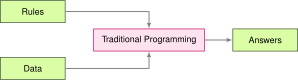](https://mlsysbook.ai/contents/core/dl_primer/2141c896d3885901604d1968bd755f4e5f07efaf.svg "Figure 3: Rule-Based Programming: Traditional programs operate on data using explicitly defined rules, forming the basis for early AI systems but lacking the adaptability of modern machine learning approaches. This approach contrasts with deep learning, where the system infers rules from examples rather than relying on pre-programmed logic.")
Figure 3: **Rule-Based Programming**: Traditional programs operate on data using explicitly defined rules, forming the basis for early AI systems but lacking the adaptability of modern machine learning approaches. This approach contrasts with deep learning, where the system infers rules from examples rather than relying on pre-programmed logic.
Despite their apparent simplicity, rule-based limitations become evident with complex real-world tasks. Recognizing human activities ([Figure 4](https://mlsysbook.ai/contents/core/dl_primer/dl_primer.html#fig-activity-rules)
) illustrates this challenge: classifying movement below 4 mph as walking seems straightforward until real-world complexity emerges. Speed variations, transitions between activities, and boundary cases each demand additional rules, creating unwieldy decision trees. Computer vision tasks compound these difficulties: detecting cats requires rules about ears, whiskers, and body shapes, while accounting for viewing angles, lighting, occlusions, and natural variations. Early systems achieved success only in controlled environments with well-defined constraints.
[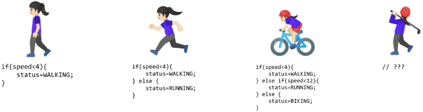](https://mlsysbook.ai/contents/core/dl_primer/images/png/activities.png "Figure 4: Rule-Based Programming: Traditional programs rely on explicitly defined rules to operate on data, forming the basis for early AI systems but lacking adaptability in complex tasks.")
Figure 4: **Rule-Based Programming**: Traditional programs rely on explicitly defined rules to operate on data, forming the basis for early AI systems but lacking adaptability in complex tasks.
Recognizing these limitations, the knowledge engineering approach that characterized artificial intelligence research in the 1970s and 1980s attempted to systematize rule creation. Expert systems[4](https://mlsysbook.ai/contents/core/dl_primer/dl_primer.html#fn4)
encoded domain knowledge as explicit rules, showing promise in specific domains with well defined parameters but struggling with tasks humans perform naturally, such as object recognition, speech understanding, or natural language interpretation. These limitations highlighted a challenge: many aspects of intelligent behavior rely on implicit knowledge that resists explicit rule based representation.
4 **Expert Systems**: Rule-based AI programs that encoded human domain expertise, prominent from 1970-1990. Notable examples include MYCIN (Stanford, 1976) for medical diagnosis, which outperformed human doctors in some antibiotics selection tasks, and XCON (DEC, 1980) for computer configuration, which saved the company $40 million annually. Despite early success, expert systems required extensive manual knowledge engineering—extracting and encoding rules from human experts—and struggled with uncertainty and common-sense reasoning that humans handle naturally.
### Classical Machine Learning
Confronting the scalability barriers of rule based systems, researchers began exploring approaches that could learn from data. Machine learning offered a promising direction: instead of writing rules for every situation, researchers could write programs that identified patterns in examples. However, the success of these methods still depended heavily on human insight to define relevant patterns, a process known as feature engineering.
This approach introduced feature engineering: transforming raw data into representations that expose patterns to learning algorithms. The Histogram of Oriented Gradients (HOG) ([Dalal and Triggs, n.d.](https://mlsysbook.ai/contents/core/dl_primer/dl_primer.html#ref-dalal2005histograms)
)[5](https://mlsysbook.ai/contents/core/dl_primer/dl_primer.html#fn5)
method ([Figure 5](https://mlsysbook.ai/contents/core/dl_primer/dl_primer.html#fig-hog)
) exemplifies this approach, identifying edges where brightness changes sharply, dividing images into cells, and measuring edge orientations within each cell. This transforms raw pixels into shape descriptors robust to lighting variations and small positional changes.
Dalal, N., and B. Triggs. n.d. “Histograms of Oriented Gradients for Human Detection.” In _2005 IEEE Computer Society Conference on Computer Vision and Pattern Recognition (CVPR’05)_, 1:886–93. IEEE; IEEE. [https://doi.org/10.1109/cvpr.2005.177](https://doi.org/10.1109/cvpr.2005.177)
.
5 **Histogram of Oriented Gradients (HOG)**: Developed by Navneet Dalal and Bill Triggs in 2005, HOG became the gold standard for object detection before deep learning. It achieved near-perfect accuracy on pedestrian detection—a breakthrough that enabled practical computer vision applications. HOG works by computing gradients (edge directions) in 8×8 pixel cells, then creating histograms of 9 orientation bins. This clever abstraction captures object shape while ignoring texture details, making it robust to lighting changes but requiring expert knowledge to design.
[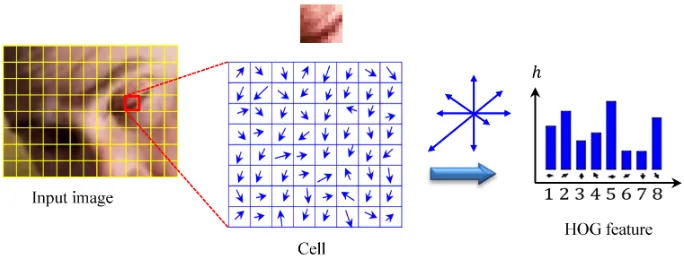](https://mlsysbook.ai/contents/core/dl_primer/images/png/hog.png "Figure 5: HOG Method: Identifies edges in images to create a histogram of gradients, transforming pixel values into shape descriptors that are invariant to lighting changes.")
Figure 5: **HOG Method**: Identifies edges in images to create a histogram of gradients, transforming pixel values into shape descriptors that are invariant to lighting changes.
Complementary methods like SIFT ([Lowe 1999](https://mlsysbook.ai/contents/core/dl_primer/dl_primer.html#ref-lowe1999object)
)[6](https://mlsysbook.ai/contents/core/dl_primer/dl_primer.html#fn6)
(Scale-Invariant Feature Transform) and Gabor filters[7](https://mlsysbook.ai/contents/core/dl_primer/dl_primer.html#fn7)
captured different visual patterns—SIFT detected keypoints stable across scale and orientation changes, while Gabor filters identified textures and frequencies. Each encoded domain expertise about visual pattern recognition.
Lowe, D. G. 1999. “Object Recognition from Local Scale-Invariant Features.” In _Proceedings of the Seventh IEEE International Conference on Computer Vision_, 2:1150–57. IEEE; IEEE. [https://doi.org/10.1109/iccv.1999.790410](https://doi.org/10.1109/iccv.1999.790410)
.
6 **Scale-Invariant Feature Transform (SIFT)**: Invented by David Lowe at University of British Columbia in 1999, SIFT revolutionized computer vision by detecting “keypoints” that remain stable across different viewpoints, scales, and lighting conditions. A typical image yields 1,000-2,000 SIFT keypoints, each described by a 128-dimensional vector. Before deep learning, SIFT was the backbone of applications like Google Street View’s image matching and early smartphone augmented reality. The algorithm’s 4-step process (scale-space extrema detection, keypoint localization, orientation assignment, and descriptor generation) required deep expertise to implement effectively.
7 **Gabor Filters**: Named after Dennis Gabor (1971 Nobel Prize in Physics for holography), these mathematical filters detect edges and textures by analyzing frequency and orientation simultaneously. Used extensively in computer vision from 1980-2010, Gabor filters mimic how the human visual cortex processes images—different neurons respond to specific orientations and spatial frequencies. A typical Gabor filter bank contains 40+ filters (8 orientations × 5 frequencies) to capture texture patterns, making them ideal for applications like fingerprint recognition and fabric quality inspection before deep learning made manual filter design obsolete.
These engineering efforts enabled advances in computer vision during the 2000s. Systems could now recognize objects with some robustness to real world variations, leading to applications in face detection, pedestrian detection, and object recognition. Despite these successes, the approach had limitations. Experts needed to carefully design feature extractors for each new problem, and the resulting features might miss important patterns that were not anticipated in their design.
### Deep Learning: Automatic Pattern Discovery
Neural networks represent a shift in how we approach problem solving with computers, establishing a new programming approach that learns from data rather than following explicit rules. This shift becomes particularly evident when considering tasks like computer vision, specifically identifying objects in images.
Deep learning differs by learning directly from raw data. Traditional programming, as we saw earlier in [Figure 3](https://mlsysbook.ai/contents/core/dl_primer/dl_primer.html#fig-traditional)
, required both rules and data as inputs to produce answers. Machine learning inverts this relationship, as shown in [Figure 6](https://mlsysbook.ai/contents/core/dl_primer/dl_primer.html#fig-deeplearning)
. Instead of writing rules, we provide examples (data) and their correct answers to discover the underlying rules automatically. This shift eliminates the need for humans to specify what patterns are important.
[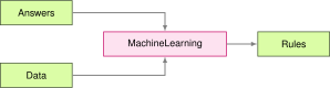](https://mlsysbook.ai/contents/core/dl_primer/6fbbdff9cc8d9f112795580e2cb59b395d80de35.svg "Figure 6: Data-Driven Rule Discovery: Deep learning models learn patterns and relationships directly from data, eliminating the need for manually specified rules and enabling automated feature extraction from raw inputs. This contrasts with traditional programming, where both rules and data are required to generate outputs, and classical machine learning, where rules are inferred from labeled data.")
Figure 6: **Data-Driven Rule Discovery**: Deep learning models learn patterns and relationships directly from data, eliminating the need for manually specified rules and enabling automated feature extraction from raw inputs. This contrasts with traditional programming, where both rules and data are required to generate outputs, and classical machine learning, where rules are inferred from labeled data.
Through this automated process, the system discovers these patterns from examples. When shown millions of images of cats, the system learns to identify increasingly complex visual patterns, from simple edges to more complex combinations that make up cat like features. This parallels how human visual systems operate, building understanding from basic visual elements to complex objects.
Building on this hierarchical learning principle, deep networks learn hierarchical representations where complex patterns emerge from simpler ones. Each layer learns increasingly abstract features: edges → shapes → objects → concepts. Deeper networks can express exponentially more functions with only polynomially more parameters, which is why “deep” matters theoretically. The compositionality principle explains why deep learning works: complex real-world patterns often have hierarchical structure that matches the network’s representational bias.
This hierarchical structure creates an advantage: unlike traditional approaches where performance plateaus, deep learning models continue improving with additional data (recognizing more variations) and computation (discovering subtler patterns). This scalability drove dramatic performance gains. Image recognition accuracy improved from 74% in 2012 to over 95% today[8](https://mlsysbook.ai/contents/core/dl_primer/dl_primer.html#fn8)
.
8 **ImageNet Competition Progress**: The ImageNet Large Scale Visual Recognition Challenge (ILSVRC) tracked computer vision progress from 2010-2017. Error rates dropped dramatically: traditional methods achieved ~28% error in 2010, AlexNet ([Krizhevsky, Sutskever, and Hinton 2017](https://mlsysbook.ai/contents/core/dl_primer/dl_primer.html#ref-krizhevsky2012imagenet)
) (first deep learning winner) achieved 15.3% in 2012, and ResNet ([He et al. 2016](https://mlsysbook.ai/contents/core/dl_primer/dl_primer.html#ref-he2016deep)
) achieved 3.6% in 2015—surpassing estimated human performance of 5.1%. This rapid improvement demonstrated deep learning’s superiority over hand-crafted features, triggering the modern AI revolution. The competition ended in 2017 when further improvements became incremental.
Krizhevsky, Alex, Ilya Sutskever, and Geoffrey E. Hinton. 2017. “ImageNet Classification with Deep Convolutional Neural Networks.” _Communications of the ACM_ 60 (6): 84–90. [https://doi.org/10.1145/3065386](https://doi.org/10.1145/3065386)
.
He, Kaiming, Xiangyu Zhang, Shaoqing Ren, and Jian Sun. 2016. “Deep Residual Learning for Image Recognition.” In _2016 IEEE Conference on Computer Vision and Pattern Recognition (CVPR)_, 770–78. IEEE. [https://doi.org/10.1109/cvpr.2016.90](https://doi.org/10.1109/cvpr.2016.90)
.
Neural network performance follows predictable scaling relationships that directly impact system design. These scaling laws explain why modern AI systems prioritize larger models over longer training: GPT-4 has ~1000× more parameters than GPT-1 but uses similar training time. Memory bandwidth and storage capacity consequently become the primary constraints rather than raw computational power. The detailed mathematical formulations of these scaling laws and their quantitative analysis are covered in **[Chapter 8: AI Training](https://mlsysbook.ai/contents/core/training/training.html#sec-ai-training)
**, while **[Chapter 10: Model Optimizations](https://mlsysbook.ai/contents/core/optimizations/optimizations.html#sec-model-optimizations)
** explores their practical implementation.
Beyond performance improvements, this approach has implications for AI system construction. Deep learning’s ability to learn directly from raw data eliminates the need for manual feature engineering while introducing new demands. Advanced infrastructure is required to handle massive datasets, powerful computers to process this data, and specialized hardware to perform complex mathematical calculations efficiently. The computational requirements of deep learning have driven the development of specialized computer chips optimized for these calculations.
The empirical evidence strongly supports these claims. The success of deep learning in computer vision exemplifies how this approach, when given sufficient data and computation, can surpass traditional methods. This pattern has repeated across many domains, from speech recognition to game playing, establishing deep learning as a transformative approach to artificial intelligence.
However, this transformation comes with trade-offs: deep learning’s computational demands reshape system requirements. Understanding these requirements provides context for the technical details of neural networks that follow.
### Computational Infrastructure Requirements
The progression from traditional programming to deep learning represents not just a shift in how we solve problems, but a transformation in computing system requirements that directly impacts every aspect of ML systems design. This transformation becomes important when we consider the full spectrum of ML systems, from massive cloud deployments to resource constrained Tiny ML devices.
Traditional programs follow predictable patterns. They execute sequential instructions, access memory in regular patterns, and use computing resources in well understood ways. A typical rule based image processing system might scan through pixels methodically, applying fixed operations with modest and predictable computational and memory requirements. These characteristics made traditional programs relatively straightforward to deploy across different computing platforms.
Table 1: **System Resource Evolution**: Programming paradigms shift system demands from sequential computation to structured parallelism with feature engineering, and finally to massive matrix operations and complex memory hierarchies in deep learning. This table clarifies how deep learning fundamentally alters system requirements compared to traditional programming and machine learning with engineered features, impacting computation and memory access patterns.
| | | | |
| --- | --- | --- | --- |
| **Computation** | Sequential, predictable paths | Structured parallel operations | Massive matrix parallelism |
| **Memory Access** | Small, predictable patterns | Medium, batch-oriented | Large, complex hierarchical patterns |
| **Data Movement** | Simple input/output flows | Structured batch processing | Intensive cross-system movement |
| **Hardware Needs** | CPU-centric | CPU with vector units | Specialized accelerators |
| **Resource Scaling** | Fixed requirements | Linear with data size | Exponential with complexity |
As we moved toward data-driven approaches, classical machine learning with engineered features introduced new complexities. Feature extraction algorithms required more intensive computation and structured data movement. The HOG feature extractor discussed earlier, for instance, requires multiple passes over image data, computing gradients and constructing histograms. While this increased both computational demands and memory complexity, the resource requirements remained predictable and scalable across platforms.
Deep learning, however, reshapes system requirements across multiple dimensions, as illustrated in [Table 1](https://mlsysbook.ai/contents/core/dl_primer/dl_primer.html#tbl-evolution)
. Understanding these evolutionary changes is important as differences manifest in several ways, with implications across the entire ML systems spectrum.
#### Parallel Matrix Operation Patterns
The computational paradigm shift becomes immediately apparent when comparing these approaches. Traditional programs follow sequential logic flows. In stark contrast, deep learning requires massive parallel operations on matrices. This shift explains why conventional CPUs, designed for sequential processing, prove inefficient for neural network computations.
This parallel computational model creates new bottlenecks. The fundamental challenge is the memory wall: while computational capacity can be increased by adding more processing units, memory bandwidth to feed those units doesn’t scale as favorably[9](https://mlsysbook.ai/contents/core/dl_primer/dl_primer.html#fn9)
. Modern accelerators address this through hierarchical memory systems with multiple cache levels and specialized memory architectures that enable data reuse. The key insight is that keeping data close to where it’s processed—in faster, smaller caches rather than slower, larger main memory—dramatically improves performance.
9 **Memory Hierarchy Performance**: Modern processors employ multiple memory levels with vastly different access speeds. L1 cache (the fastest, closest to processor) provides data in 1-2 processor clock cycles, L2 cache requires 10-20 cycles, while main memory takes 100+ cycles—creating a 50-100× speed difference. The throughput also varies dramatically: L1 can deliver up to ~1000 GB/s (gigabytes per second), L2 up to ~500 GB/s, while main memory provides only ~100 GB/s on CPUs (~1 TB/s on GPUs with specialized high-bandwidth memory). Neural network accelerators succeed by keeping frequently accessed weights in fast cache and reusing them across many computations, often achieving 80%+ cache hit rates through careful scheduling.
These memory hierarchy challenges explain why neural network accelerators focus on maximizing data reuse. Rather than repeatedly fetching the same weights from slow main memory, successful designs keep frequently accessed data in fast local storage and carefully schedule operations to minimize data movement. The detailed quantitative analysis of these memory systems and their performance characteristics is covered in **[Chapter 11: AI Acceleration](https://mlsysbook.ai/contents/core/hw_acceleration/hw_acceleration.html#sec-ai-acceleration)
**.
The need for parallel processing has driven the adoption of specialized hardware architectures, ranging from powerful cloud GPUs to specialized mobile processors to Tiny ML accelerators. The specific hardware architectures and their trade-offs for ML workloads are explored in **[Chapter 11: AI Acceleration](https://mlsysbook.ai/contents/core/hw_acceleration/hw_acceleration.html#sec-ai-acceleration)
**.
#### Hierarchical Memory Architecture
The memory requirements present another shift. Traditional programs typically maintain small, fixed memory footprints. In contrast, deep learning models must manage parameters across complex memory hierarchies. Memory bandwidth often becomes the primary performance bottleneck, creating challenges for resource-constrained systems.
This memory-intensive nature creates performance bottlenecks unique to neural computing. Matrix multiplication—the core neural network operation—is often memory bandwidth-bound rather than compute-bound[10](https://mlsysbook.ai/contents/core/dl_primer/dl_primer.html#fn10)
. The fundamental issue is that processors can perform computations faster than they can fetch data from memory. Each weight must be loaded from memory to perform a multiplication, and if the memory system can’t supply data fast enough, computational units sit idle waiting for values to arrive. This imbalance between computational capability and memory bandwidth explains why simply adding more processing units doesn’t proportionally improve performance.
10 **Memory-Bound Operations**: Consider a typical matrix multiplication: a processor capable of performing a billion floating-point operations per second requires loading data at 250-500 GB/s (gigabytes per second) to keep computational units fully utilized. However, typical CPU memory bandwidth is only 50-100 GB/s, while even high-end GPUs provide 1-2 TB/s (terabytes per second). This gap means CPUs achieve only 5-15% of peak computational efficiency on neural network operations, while GPUs reach 40-60% through higher bandwidth and better data reuse strategies.
GPUs address this challenge through both higher memory bandwidth and massive parallelism, achieving better utilization than traditional CPUs. However, the underlying constraint remains: energy consumption in neural networks is dominated by data movement, not computation. Moving data from main memory to processing units consumes more energy than the actual mathematical operations. This energy hierarchy explains why specialized processors focus on techniques that reduce data movement, keeping data closer to where it’s processed.
This fundamental memory-computation tradeoff manifests differently across deployment scenarios. Cloud servers can afford more memory and power to maximize throughput, while mobile devices must carefully optimize to operate within strict power budgets. Training systems prioritize computational throughput even at higher energy costs, while inference systems emphasize energy efficiency. These different constraints drive different optimization strategies across the ML systems spectrum, ranging from memory-rich cloud deployments to heavily optimized Tiny ML implementations.
Memory optimization strategies like quantization and pruning are detailed in **[Chapter 10: Model Optimizations](https://mlsysbook.ai/contents/core/optimizations/optimizations.html#sec-model-optimizations)
**, while hardware architectures and their memory systems are explored in **[Chapter 11: AI Acceleration](https://mlsysbook.ai/contents/core/hw_acceleration/hw_acceleration.html#sec-ai-acceleration)
**.
#### Distributed Computing Requirements
Researchers discovered deep learning changes how systems scale and the importance of efficiency. Traditional programs have relatively fixed resource requirements with predictable performance characteristics. Deep learning models can consume exponentially more resources as they grow in complexity. This relationship between model capability and resource consumption makes system efficiency a concern. **[Chapter 9: Efficient AI](https://mlsysbook.ai/contents/core/efficient_ai/efficient_ai.html#sec-efficient-ai)
** provides coverage of techniques to optimize this relationship, including methods to reduce computational requirements while maintaining model performance.
Bridging algorithmic concepts with hardware realities becomes essential. While traditional programs map relatively straightforwardly to standard computer architectures, deep learning requires careful consideration of:
* How to efficiently map matrix operations to physical hardware (**[Chapter 11: AI Acceleration](https://mlsysbook.ai/contents/core/hw_acceleration/hw_acceleration.html#sec-ai-acceleration)
** covers hardware-specific optimization strategies)
* Ways to minimize data movement across memory hierarchies
* Methods to balance computational capability with resource constraints (**[Chapter 9: Efficient AI](https://mlsysbook.ai/contents/core/efficient_ai/efficient_ai.html#sec-efficient-ai)
** explores scaling laws and efficiency trade-offs)
* Techniques to optimize both algorithm and system-level efficiency (**[Chapter 10: Model Optimizations](https://mlsysbook.ai/contents/core/optimizations/optimizations.html#sec-model-optimizations)
** provides model compression techniques)
These shifts explain why deep learning has spurred innovations across the entire computing stack. From specialized hardware accelerators to new memory architectures to sophisticated software frameworks, the demands of deep learning continue to reshape computer system design.
Having established both the historical progression from rule-based systems to neural networks and the computational infrastructure this evolution demands, we now examine the foundational inspiration behind these systems. The answer to what neural networks compute begins not with silicon and software, but with biology—specifically, the neural networks in our brains that inspired the artificial neural networks powering modern AI systems.
**Self-Check: Question 1.2**
1. Which of the following best describes a limitation of rule-based systems that led to the development of machine learning?
1. Rule-based systems are too complex to implement.
2. Rule-based systems require too much computational power.
3. Rule-based systems cannot adapt to new data without manual updates.
4. Rule-based systems are not interpretable.
2. Explain how deep learning differs from classical machine learning in terms of feature extraction.
3. What is a key system-level implication of adopting deep learning over traditional programming?
1. Deep learning requires less data movement across memory hierarchies.
2. Deep learning models have fixed resource requirements.
3. Deep learning simplifies the deployment of ML systems.
4. Deep learning necessitates specialized hardware for efficient computation.
4. In a production system, what trade-offs might you consider when choosing between classical machine learning and deep learning?
[See Answers →](https://mlsysbook.ai/contents/core/dl_primer/dl_primer.html#quiz-answer-sec-dl-primer-evolution-ml-paradigms-e0a4)
From Biology to Silicon
-----------------------
Having examined how programming approaches evolved from rules to data-driven learning, and how this evolution drives the computational infrastructure requirements we see today, we now turn to the question: what are these neural networks actually computing? The answer begins not with silicon, but with biology.
The massive computational requirements we just examined (specialized processors, hierarchical memory systems, high-bandwidth data movement) all trace back to a simple inspiration: the biological neuron. Understanding how nature solves information processing problems with 20 watts of power reveals both the potential and the challenges of artificial neural systems. As we examine biological neurons and their artificial counterparts, watch for a pattern: each biological feature that we choose to implement or approximate creates specific computational demands, linking the dendrite-and-synapse model directly to the processing power and memory bandwidth requirements we just discussed.
This section bridges biological inspiration and systems implementation by examining three key transformations: how biological neurons inspire artificial neuron design, how neural principles translate into mathematical operations, and how these operations drive the system requirements we outlined earlier. By the end, you’ll understand why implementing even simplified neural computation requires the specialized hardware infrastructure modern ML systems demand.
### Biological Neural Processing Principles
From a systems perspective, biological neural networks offer solutions to the computational challenges we’ve just discussed: they achieve massive parallelism, efficient memory usage, and adaptive learning while consuming minimal energy. Four key principles from biological intelligence directly inform artificial neural network design:
**Adaptive Learning**: The brain continuously modifies neural connections based on experience, refining responses through interaction with the environment. This biological capability inspired machine learning’s core principle: improving from data rather than following fixed, pre-programmed rules.
**Parallel Processing**: The brain processes vast amounts of information simultaneously, with different regions specializing in specific functions while working in concert. This distributed, parallel architecture contrasts with traditional sequential computing and has influenced modern AI system design.
**Pattern Recognition**: Biological systems excel at identifying patterns in complex, noisy data—recognizing faces in crowds, understanding speech in noisy environments, identifying objects from partial information. This capability has inspired applications in computer vision and speech recognition, though artificial systems still strive to match the brain’s efficiency.
**Energy Efficiency**: Biological systems achieve processing with exceptional energy efficiency. The human brain’s 20-watt power consumption[11](https://mlsysbook.ai/contents/core/dl_primer/dl_primer.html#fn11)
creates a stark efficiency gap that artificial systems are still striving to bridge. Understanding and replicating this efficiency is explored in **[Chapter 18: Sustainable AI](https://mlsysbook.ai/contents/core/sustainable_ai/sustainable_ai.html#sec-sustainable-ai)
** through environmental impact analysis and energy-efficient optimization strategies.
11 **Brain Energy Efficiency**: The human brain contains approximately 86-100 billion neurons and performs an estimated 10^13 to 10^16 operations per second on just 20 watts—equivalent to running a single LED light bulb. In contrast, training GPT-3 ([Brown et al. 2020](https://mlsysbook.ai/contents/core/dl_primer/dl_primer.html#ref-brown2020language)
) consumed about 1,287 megawatt-hours of electricity ([Strubell, Ganesh, and McCallum 2019](https://mlsysbook.ai/contents/core/dl_primer/dl_primer.html#ref-strubell2019energy)
). This stark efficiency gap drives research into neuromorphic computing and inspired the development of specialized AI chips designed to mimic brain-like processing.
Brown, Tom, Benjamin Mann, Nick Ryder, Melanie Subbiah, Jared D Kaplan, Prafulla Dhariwal, Arvind Neelakantan, et al. 2020. “Language Models Are Few-Shot Learners.” _Advances in Neural Information Processing Systems_ 33: 1877–1901.
Strubell, Emma, Ananya Ganesh, and Andrew McCallum. 2019. “Energy and Policy Considerations for Deep Learning in NLP.” In _Proceedings of the 57th Annual Meeting of the Association for Computational Linguistics_, 3645–50. Association for Computational Linguistics. [https://doi.org/10.18653/v1/p19-1355](https://doi.org/10.18653/v1/p19-1355)
.
These biological principles suggest key requirements for artificial neural systems: simple processing units integrating multiple inputs, adjustable connection strengths, nonlinear activation based on input thresholds, parallel processing architecture, and learning through connection strength modification. The following sections examine how we translate these biological insights into mathematical operations and into silicon implementations.
These biological principles have shaped two approaches in artificial intelligence. The first attempts to directly mimic neural structure and function, creating artificial neural networks that structurally resemble biological networks. The second takes a more abstract approach, adapting biological principles to work efficiently within computer hardware constraints without copying biological structures exactly.
To understand how either approach works in practice, we must first examine the basic unit that makes neural computation possible: the individual neuron. By understanding how biological neurons process information, we can then see how this process translates into the mathematical operations that drive artificial neural networks.
### Biological Neuron Structure
Translating these high-level principles into practical implementation requires examining the basic unit of biological information processing: the neuron. This cellular building block provides the blueprint for its artificial counterpart and reveals how complex neural networks emerge from simple components working together.
In biological systems, the neuron (or cell) represents the basic functional unit of the nervous system. Understanding its structure is crucial for drawing parallels to artificial systems. [Figure 7](https://mlsysbook.ai/contents/core/dl_primer/dl_primer.html#fig-bio_nn2ai_nn)
illustrates the structure of a biological neuron.
[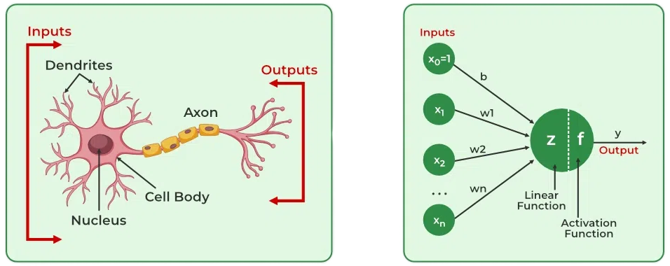](https://mlsysbook.ai/contents/core/dl_primer/images/png/bio_nn2ai_nn.png "Figure 7: Biological Neuron Mapping: Artificial neurons abstract key functions from their biological counterparts, receiving weighted inputs at dendrites, summing them in the cell body, and producing an output via the axon, analogous to activation functions in artificial neural networks. This abstraction enables the construction of complex artificial neural networks capable of sophisticated information processing. Source: geeksforgeeks.")
Figure 7: **Biological Neuron Mapping**: Artificial neurons abstract key functions from their biological counterparts, receiving weighted inputs at dendrites, summing them in the cell body, and producing an output via the axon, analogous to activation functions in artificial neural networks. This abstraction enables the construction of complex artificial neural networks capable of sophisticated information processing. Source: geeksforgeeks.
A biological neuron consists of several key components. The central part is the cell body, or soma, which contains the nucleus and performs the cell’s basic life processes. Extending from the soma are branch-like structures called dendrites, which act as receivers for incoming signals from other neurons. The connections between neurons occur at synapses[12](https://mlsysbook.ai/contents/core/dl_primer/dl_primer.html#fn12)
, which modulate the strength of the transmitted signals. Finally, a long, slender projection called the axon conducts electrical impulses away from the cell body to other neurons.
12 **Synapses**: From the Greek word “synaptein” meaning “to clasp together,” synapses are the connection points between neurons where chemical or electrical signals are transmitted. A typical neuron has 1,000-10,000 synaptic connections, and the human brain contains roughly 100 trillion synapses. The strength of synaptic connections can change through experience, forming the biological basis of learning and memory—a principle directly mimicked by adjustable weights in artificial neural networks.
Integrating these structural components, the neuron functions as follows: Dendrites act as receivers, collecting input signals from other neurons. Synapses at these connections modulate the strength of each signal, determining how much influence each input has. The soma integrates these weighted signals and decides whether to trigger an output signal. If triggered, the axon transmits this signal to other neurons.
Each element of a biological neuron has a computational analog in artificial systems, reflecting the principles of learning, adaptability, and efficiency found in nature. To better understand how biological intelligence informs artificial systems, [Table 2](https://mlsysbook.ai/contents/core/dl_primer/dl_primer.html#tbl-bio_nn2ai_nn)
captures the mapping between the components of biological and artificial neurons. This should be viewed alongside [Figure 7](https://mlsysbook.ai/contents/core/dl_primer/dl_primer.html#fig-bio_nn2ai_nn)
for a complete picture. Together, they show the biological-to-artificial neuron mapping.
Table 2: **Neuron Correspondence**: Biological neurons inspire artificial neuron design through analogous components—dendrites map to inputs (receiving signals), synapses map to weights (modulating connection strength), the soma to net input, and the axon to output—establishing a foundation for computational modeling of intelligence. This table clarifies how key functions of biological neurons are abstracted and implemented in artificial neural networks, enabling learning and information processing.
| | |
| --- | --- |
| **Cell** | Neuron / Node |
| **Dendrites** | Inputs |
| **Synapses** | Weights |
| **Soma** | Net Input |
| **Axon** | Output |
Understanding these correspondences proves crucial for grasping how artificial systems approximate biological intelligence. Each component serves a similar function through different mechanisms, with specific implications for artificial neural networks.
1. **Cell \\(\\longleftrightarrow\\) Neuron/Node**: The artificial neuron or node serves as the basic computational unit, mirroring the cell’s role in biological systems.
2. **Dendrites \\(\\longleftrightarrow\\) Inputs**: Dendrites in biological neurons receive incoming signals from other neurons, analogous to how inputs feed into artificial neurons. They act as the signal receivers, like antennas collecting information.
3. **Synapses \\(\\longleftrightarrow\\) Weights**: Synapses modulate the strength of connections between neurons, directly analogous to weights in artificial neurons. These weights are adjustable, enabling learning and optimization over time by controlling how much influence each input has.
4. **Soma \\(\\longleftrightarrow\\) Net Input**: The net input in artificial neurons sums weighted inputs to determine activation, similar to how the soma integrates signals in biological neurons.
5. **Axon \\(\\longleftrightarrow\\) Output**: The output of an artificial neuron passes processed information to subsequent network layers, much like an axon transmits signals to other neurons.
This mapping illustrates how artificial neural networks simplify and abstract biological processes while preserving their essential computational principles. Understanding individual neurons represents only the beginning. The true power of neural networks emerges from how these basic units work together in larger systems.
From a systems engineering perspective, this biological-to-artificial translation reveals why neural networks have such demanding computational requirements. Each simple biological process maps to intensive mathematical operations that must be executed millions or billions of times in parallel.
### Artificial Neural Network Design Principles
Bridging the gap from biological inspiration to practical implementation, the translation from biological principles to artificial computation requires a deep appreciation of what makes biological neural networks so effective at both the cellular and network levels, and why replicating these capabilities in silicon presents such significant systems challenges. The brain processes information through distributed computation across billions of neurons, each operating relatively slowly compared to silicon transistors. A biological neuron fires at approximately 200 Hz, while modern processors operate at gigahertz frequencies. Despite this speed limitation, the brain’s parallel architecture enables sophisticated real-time processing of complex sensory input, decision-making, and control of behavior.
Despite the apparent speed disadvantage, this computational efficiency emerges from the brain’s basic organizational principles. Each neuron acts as a simple processing unit, integrating inputs from thousands of other neurons and producing a binary output signal based on whether this integrated input exceeds a threshold. The connection strengths between neurons, mediated by synapses, are continuously modified through experience. This synaptic plasticity forms the basis for learning and adaptation in biological neural networks.
Replicating biological efficiency in artificial systems requires navigating fundamental trade-offs. While the brain achieves remarkable efficiency with only 20 watts (as noted earlier), comparable artificial neural networks require orders of magnitude more power. Large language models, for example, can consume megawatts during training and kilowatts during inference—thousands to hundreds of thousands of times more power than the brain. This substantial efficiency gap drives the engineering focus on specialized hardware, quantization techniques, and architectural innovations.
Drawing from these organizational insights, biological systems suggest several key computational elements needed in artificial neural systems:
* Simple processing units that integrate multiple inputs
* Adjustable connection strengths between units
* Nonlinear activation based on input thresholds
* Parallel processing architecture
* Learning through modification of connection strengths
The question now becomes: how do we translate these abstract biological principles into concrete mathematical operations that computers can execute?
### Mathematical Translation of Neural Concepts
Translating biological insights into practical systems, we face the challenge of capturing the essence of neural computation within the rigid framework of digital systems. As established in our neuron model analysis (see [Table 2](https://mlsysbook.ai/contents/core/dl_primer/dl_primer.html#tbl-bio_nn2ai_nn)
), artificial neurons simplify biological processes into three key operations: weighted input processing (synaptic strength), summation (signal integration), and activation functions (threshold-based firing).
[Table 3](https://mlsysbook.ai/contents/core/dl_primer/dl_primer.html#tbl-bio2comp)
provides a systematic view of how these biological features map to their computational counterparts, revealing both the possibilities and limitations of digital neural implementation.
Table 3: **Biological-Computational Analogies**: Artificial neurons abstract key principles of biological neural systems, mapping neuron firing to activation functions, synaptic strength to weighted connections, and signal integration to summation operations—establishing a foundation for digital neural implementation. Distributed memory and parallel processing in biological systems find computational counterparts in weight matrices and concurrent computation, respectively, highlighting both the power and limitations of this abstraction.
| | |
| --- | --- |
| **Neuron firing** | Activation function |
| **Synaptic strength** | Weighted connections |
| **Signal integration** | Summation operation |
| **Distributed memory** | Weight matrices |
| **Parallel processing** | Concurrent computation |
Using the biological-to-artificial mapping principles outlined earlier, this mathematical abstraction preserves key computational principles while enabling efficient digital implementation. The weighting, summation, and activation operations directly correspond to the synaptic strength, signal integration, and threshold firing mechanisms identified in our neuron correspondence analysis.
This abstraction has a computational cost. What happens effortlessly in biology requires intensive mathematical computation in artificial systems. As discussed in the Memory Systems section, these operations create significant computational demands due to memory bandwidth limitations.
Memory in artificial neural networks takes a markedly different form from biological systems. While biological memories are distributed across synaptic connections and neural patterns, artificial networks store information in discrete weights and parameters. This architectural difference reflects the constraints of current computing hardware, where memory and processing are physically separated rather than integrated as in biological systems. Despite these implementation differences, artificial neural networks achieve similar functional capabilities in pattern recognition and learning.
The brain’s massive parallelism represents a challenge in artificial implementation. While biological neural networks process information through billions of neurons operating simultaneously, artificial systems approximate this parallelism through specialized hardware like GPUs and tensor processing units. These devices efficiently compute the matrix operations that form the mathematical foundation of artificial neural networks, achieving parallel processing at a different scale and granularity than biological systems.
### Hardware and Software Requirements
The computational translation of neural principles creates infrastructure demands that emerge from key differences between biological and artificial implementations, directly shaping system design.
[Table 4](https://mlsysbook.ai/contents/core/dl_primer/dl_primer.html#tbl-comp2sys)
shows how each computational element drives particular system requirements. This mapping shows how the choices made in computational translation directly influence the hardware and system architecture needed for implementation.
Table 4: **Computational Demands**: Artificial neural network design directly translates into specific system requirements; for example, efficient activation functions necessitate fast nonlinear operation units and large-scale weight storage demands high-bandwidth memory access. Understanding this mapping guides hardware and system architecture choices for effective implementation of artificial intelligence.
| | |
| --- | --- |
| **Activation functions** | Fast nonlinear operation units |
| **Weight operations** | High-bandwidth memory access |
| **Parallel computation** | Specialized parallel processors |
| **Weight storage** | Large-scale memory systems |
| **Learning algorithms** | Gradient computation hardware |
Storage architecture represents a critical requirement, driven by the key difference in how biological and artificial systems handle memory. In biological systems, memory and processing are intrinsically integrated—synapses both store connection strengths and process signals. Artificial systems, however, must maintain a clear separation between processing units and memory. This creates a need for both high-capacity storage to hold millions or billions of connection weights and high-bandwidth pathways to move this data quickly between storage and processing units. The efficiency of this data movement often becomes a critical bottleneck that biological systems do not face.
The learning process itself imposes distinct requirements on artificial systems. While biological networks modify synaptic strengths through local chemical processes, artificial networks must coordinate weight updates across the entire network. This creates computational and memory demands during training, as systems must not only store current weights but also maintain space for gradients and intermediate calculations. The requirement to backpropagate error signals, with no real biological analog, complicates the system architecture. Securing these large models and protecting sensitive training data introduces complex requirements addressed in **[Chapter 16: Robust AI](https://mlsysbook.ai/contents/core/robust_ai/robust_ai.html#sec-robust-ai)
**.
Energy efficiency emerges as a final critical requirement, highlighting perhaps the starkest contrast between biological and artificial implementations. The human brain’s remarkable energy efficiency, which operates on approximately 20 watts, stands in sharp contrast to the substantial power demands of artificial neural networks. Current systems often require orders of magnitude more energy to implement similar capabilities. This gap drives ongoing research in more efficient hardware architectures and has profound implications for the practical deployment of neural networks, particularly in resource-constrained environments like mobile devices or edge computing systems. The environmental impact of this energy consumption and strategies for sustainable AI development are explored in **[Chapter 18: Sustainable AI](https://mlsysbook.ai/contents/core/sustainable_ai/sustainable_ai.html#sec-sustainable-ai)
**.
These system requirements directly drive the architectural choices we make in building ML systems, from the specialized hardware accelerators covered in **[Chapter 11: AI Acceleration](https://mlsysbook.ai/contents/core/hw_acceleration/hw_acceleration.html#sec-ai-acceleration)
** to the distributed training systems discussed in **[Chapter 8: AI Training](https://mlsysbook.ai/contents/core/training/training.html#sec-ai-training)
**. Understanding why these requirements exist, rooted in the key differences between biological and artificial computation, is essential for making informed decisions about system design and optimization.
### Evolution of Neural Network Computing
We can appreciate how the field of deep learning evolved to meet these challenges through advances in hardware and algorithms. This journey began with early artificial neural networks in the 1950s, marked by the introduction of the Perceptron ([Rosenblatt 1958](https://mlsysbook.ai/contents/core/dl_primer/dl_primer.html#ref-rosenblatt1958perceptron)
)[13](https://mlsysbook.ai/contents/core/dl_primer/dl_primer.html#fn13)
. While groundbreaking in concept, these early systems were severely limited by the computational capabilities of their era, primarily mainframe computers that lacked both the processing power and memory capacity needed for complex networks.
Rosenblatt, F. 1958. “The Perceptron: A Probabilistic Model for Information Storage and Organization in the Brain.” _Psychological Review_ 65 (6): 386–408. [https://doi.org/10.1037/h0042519](https://doi.org/10.1037/h0042519)
.
13 **Perceptron**: Invented by Frank Rosenblatt in 1957 at Cornell, the perceptron was the first artificial neural network capable of learning. The New York Times famously reported it would be “the embryo of an electronic computer that \[the Navy\] expects will be able to walk, talk, see, write, reproduce itself and be conscious of its existence.” While overly optimistic, this breakthrough laid the foundation for all modern neural networks.
Rumelhart, David E., Geoffrey E. Hinton, and Ronald J. Williams. 1986. “Learning Representations by Back-Propagating Errors.” _Nature_ 323 (6088): 533–36. [https://doi.org/10.1038/323533a0](https://doi.org/10.1038/323533a0)
.
14 **Backpropagation**: Published by Rumelhart, Hinton, and Williams in 1986, backpropagation solved the “credit assignment problem” (how to determine which weights in a multi-layer network were responsible for errors). This algorithm, based on the mathematical chain rule, enabled training of deep networks and directly led to the modern AI revolution. A similar algorithm was discovered by Paul Werbos in 1974 but went largely unnoticed.
The development of backpropagation algorithms in the 1980s ([Rumelhart, Hinton, and Williams 1986](https://mlsysbook.ai/contents/core/dl_primer/dl_primer.html#ref-rumelhart1986learning)
) was a theoretical breakthrough[14](https://mlsysbook.ai/contents/core/dl_primer/dl_primer.html#fn14)
and provided a systematic way to train multi-layer networks. The computational demands of this algorithm far exceeded available hardware capabilities. Training even modest networks could take weeks, making experimentation and practical applications challenging. This mismatch between algorithmic requirements and hardware capabilities contributed to a period of reduced interest in neural networks.
[](https://mlsysbook.ai/contents/core/dl_primer/images/png/trends_65d82031.png "Figure 8: Computational Growth: Exponential increases in computational power—initially at a 1.4× rate from 1952–2010, then accelerating to a doubling every 3.4 months from 2012–2022—enabled the scaling of deep learning models. this trend, coupled with a 10-month doubling cycle for large-scale models after 2015, directly addresses the historical bottleneck of training complex neural networks and fueled the recent advances in the field. Source: [@epochai2023trends].")
Figure 8: **Computational Growth**: Exponential increases in computational power—initially at a 1.4× rate from 1952–2010, then accelerating to a doubling every 3.4 months from 2012–2022—enabled the scaling of deep learning models. this trend, coupled with a 10-month doubling cycle for large-scale models after 2015, directly addresses the historical bottleneck of training complex neural networks and fueled the recent advances in the field. Source: ([Sardanelli et al. 2023](https://mlsysbook.ai/contents/core/dl_primer/dl_primer.html#ref-epochai2023trends)
).
Sardanelli, Francesco, Isabella Castiglioni, Anna Colarieti, Simone Schiaffino, and Giovanni Di Leo. 2023. “Artificial Intelligence (AI) in Biomedical Research: Discussion on Authors’ Declaration of AI in Their Articles Title.” _European Radiology Experimental_ 7 (1): 2. [https://doi.org/10.1186/s41747-022-00316-7](https://doi.org/10.1186/s41747-022-00316-7)
.
While we’ve established the technical foundations of deep learning in earlier sections, the term itself gained prominence in the 2010s, coinciding with significant advances in computational power and data accessibility. The field has grown exponentially, as illustrated in [Figure 8](https://mlsysbook.ai/contents/core/dl_primer/dl_primer.html#fig-trends)
. The graph reveals two remarkable trends: computational capabilities measured in floating-point operations per second (FLOPS) initially followed a \\(1.4\\times\\) improvement pattern from 1952 to 2010, then accelerated to a 3.4-month doubling cycle from 2012 to 2022. Perhaps more striking is the emergence of large-scale models between 2015 and 2022 (not explicitly shown or easily seen in the figure), which scaled 2 to 3 orders of magnitude faster than the general trend, following an aggressive 10-month doubling cycle.
The evolutionary trends were driven by parallel advances across three dimensions: data availability, algorithmic innovations, and computing infrastructure. These three factors reinforced each other in a virtuous cycle that continues to drive progress in the field today. As [Figure 9](https://mlsysbook.ai/contents/core/dl_primer/dl_primer.html#fig-virtuous-cycle)
shows, more powerful computing infrastructure enabled processing larger datasets. Larger datasets drove algorithmic innovations. Better algorithms demanded more sophisticated computing systems.
[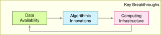](https://mlsysbook.ai/contents/core/dl_primer/df0674b614a5746ac9435d8d82b3ec5711780d1e.svg "Figure 9: ")
Figure 9
The data revolution transformed what was possible with neural networks. The rise of the internet and digital devices created unprecedented access to training data. Image sharing platforms provided millions of labeled images. Digital text collections enabled language processing at scale. Sensor networks and IoT devices generated continuous streams of real-world data. This abundance of data provided the raw material needed for neural networks to learn complex patterns effectively.
Algorithmic innovations made it possible to use this data effectively. New methods for initializing networks and controlling learning rates made training more stable. Techniques for preventing overfitting[15](https://mlsysbook.ai/contents/core/dl_primer/dl_primer.html#fn15)
allowed models to generalize better to new data. Researchers discovered that neural network performance scaled predictably with model size, computation, and data quantity, leading to increasingly ambitious architectures.
15 **Overfitting**: When a model memorizes training examples instead of learning generalizable patterns—like a student who memorizes answers instead of understanding concepts. The model performs perfectly on training data but fails on new examples. Common signs include training accuracy continuing to improve while validation accuracy plateaus or decreases. Think of it as becoming an “expert” on a practice test who panics when facing slightly different questions on the real exam.
16 **Tensor Processing Unit (TPU)**: Google’s custom silicon designed specifically for tensor operations, the mathematical building blocks of neural networks. First deployed internally in 2015, TPUs can perform matrix multiplications up to 30× faster than 2015-era GPUs while using less power. The name reflects their optimization for tensor operations—multi-dimensional arrays that represent data flowing through neural networks. Google has since made TPUs available through cloud services, democratizing access to this specialized AI hardware.
Jouppi, Norman P., Cliff Young, Nishant Patil, David Patterson, Gaurav Agrawal, Raminder Bajwa, Sarah Bates, et al. 2017. “In-Datacenter Performance Analysis of a Tensor Processing Unit.” In _Proceedings of the 44th Annual International Symposium on Computer Architecture_, 1–12. ISCA ’17. New York, NY, USA: ACM. [https://doi.org/10.1145/3079856.3080246](https://doi.org/10.1145/3079856.3080246)
.
17 **Deep Learning Frameworks**: TensorFlow ([Abadi et al. 2016](https://mlsysbook.ai/contents/core/dl_primer/dl_primer.html#ref-abadi2016tensorflow)
) (released by Google in 2015) and PyTorch ([Paszke et al. 2019](https://mlsysbook.ai/contents/core/dl_primer/dl_primer.html#ref-paszke2019pytorch)
) (released by Facebook in 2016) democratized deep learning by handling the complex mathematics automatically. Before these frameworks, implementing backpropagation required writing hundreds of lines of error-prone calculus code. Now, a complete neural network can be defined in 10-20 lines. TensorFlow emphasizes production deployment and has been downloaded over 180 million times, while PyTorch dominates research with its dynamic computation graphs. These frameworks automatically compute gradients, optimize GPU memory usage, and distribute training across multiple machines.
Abadi, Martín, Ashish Agarwal, Paul Barham, Eugene Brevdo, Zhifeng Chen, Craig Citro, Greg S. Corrado, et al. 2016. “TensorFlow: Large-Scale Machine Learning on Heterogeneous Distributed Systems.” _arXiv Preprint arXiv:1603.04467_, March. [http://arxiv.org/abs/1603.04467v2](http://arxiv.org/abs/1603.04467v2)
.
Paszke, Adam, Sam Gross, Francisco Massa, Adam Lerer, James Bradbury, Gregory Chanan, Trevor Killeen, et al. 2019. “PyTorch: An Imperative Style, High-Performance Deep Learning Library.” In _Advances in Neural Information Processing Systems_, 32:8024–35.
Computing infrastructure evolved to meet these growing demands. On the hardware side, graphics processing units (GPUs) provided the parallel processing capabilities needed for efficient neural network computation. Specialized AI accelerators like TPUs[16](https://mlsysbook.ai/contents/core/dl_primer/dl_primer.html#fn16)
([Jouppi et al. 2017](https://mlsysbook.ai/contents/core/dl_primer/dl_primer.html#ref-jouppi2017datacenter)
) pushed performance further. High-bandwidth memory systems and fast interconnects addressed data movement challenges. Equally important were software advances—frameworks and libraries[17](https://mlsysbook.ai/contents/core/dl_primer/dl_primer.html#fn17)
that made it easier to build and train networks, distributed computing systems that enabled training at scale, and tools for optimizing model deployment.
The convergence of data availability, algorithmic innovation, and computational infrastructure created the foundation for modern deep learning. Building effective ML systems requires understanding the computational operations that drive infrastructure requirements. Simple mathematical operations, when scaled across millions of parameters and billions of training examples, create the massive computational demands that shaped this evolution.
**Self-Check: Question 1.3**
1. Which component of a biological neuron corresponds to the ‘weights’ in an artificial neuron?
1. Dendrites
2. Axon
3. Soma
4. Synapses
2. Explain how the principle of parallel processing in biological systems influences the design of artificial neural networks.
3. What is a key system requirement driven by the need for high-bandwidth memory access in artificial neural networks?
1. Fast nonlinear operation units
2. Large-scale memory systems
3. Specialized parallel processors
4. Gradient computation hardware
4. The human brain’s energy efficiency, operating on approximately 20 watts, highlights the need for more efficient hardware architectures in artificial systems. This efficiency gap is a driving force behind research into \_\_\_\_\_\_\_.
5. In a production system, what trade-offs might you consider when choosing between a biologically inspired neural network design and a more abstract computational model?
[See Answers →](https://mlsysbook.ai/contents/core/dl_primer/dl_primer.html#quiz-answer-sec-dl-primer-biology-silicon-0482)
Neural Network Fundamentals
---------------------------
Having traced neural networks’ evolution from biological inspiration through historical milestones to modern systems, we now shift focus from “why deep learning succeeded” to “how neural networks actually compute.” This section develops the mathematical and architectural foundations essential for ML systems engineering.
We take a bottom-up approach, building from simple to complex: individual neurons that perform weighted summations → layers that organize parallel computation → complete networks that transform raw inputs into predictions. Each concept introduces both mathematical principles and their systems implications. As you read, notice how each seemingly simple operation—a dot product here, an activation function there—compounds into the computational requirements we discussed earlier: millions of parameters demanding gigabytes of memory, billions of operations requiring specialized hardware, massive datasets necessitating distributed training.
The latest developments in neural architectures and emerging paradigms that build upon these foundations are explored in **[Chapter 20: AGI Systems](https://mlsysbook.ai/contents/core/frontiers/frontiers.html#sec-agi-systems)
**. For now, we establish the foundational concepts that all neural networks share, from simple classifiers to large language models.
### Network Architecture Fundamentals
The architecture of a neural network determines how information flows through the system, from input to output. While modern networks can be tremendously complex, they all build upon a few key organizational principles that directly impact system design. Understanding these principles is necessary for both implementing neural networks and appreciating why they require the computational infrastructure we’ve discussed.
To ground these concepts in a concrete example, we’ll use handwritten digit recognition throughout this section—specifically, the task of classifying images from the MNIST dataset ([Lecun et al. 1998](https://mlsysbook.ai/contents/core/dl_primer/dl_primer.html#ref-lecun1998gradient)
). This seemingly simple task reveals all the fundamental principles of neural networks while providing intuition for more complex applications.
**Example:** Running Example: MNIST Digit Recognition
**The Task**: Given a 28×28 pixel grayscale image of a handwritten digit, classify it as one of the ten digits (0-9).
**Input Representation**: Each image contains 784 pixels (28×28), with values ranging from 0 (white) to 255 (black). We normalize these to the range \[0,1\] by dividing by 255. When fed to a neural network, these 784 values form our input vector \\(\\mathbf{x} \\in \\mathbb{R}^{784}\\).
**Output Representation**: The network produces 10 values, one for each possible digit. These values represent the network’s confidence that the input image contains each digit. The digit with the highest confidence becomes the prediction.
**Why This Example**: MNIST is small enough to understand completely (784 inputs, ~100K parameters for a simple network) yet large enough to be realistic. The task is intuitive—everyone understands what “recognize a handwritten 7” means—making it ideal for learning neural network principles that scale to much larger problems.
**Network Architecture Preview**: A typical MNIST classifier might use: 784 input neurons (one per pixel) → 128 hidden neurons → 64 hidden neurons → 10 output neurons (one per digit class). As we develop concepts, we’ll reference this specific architecture.
Driving practical system design, each architectural choice—from how neurons are connected to how layers are organized—creates specific computational patterns that must be efficiently mapped to hardware. This mapping between network architecture and computational requirements is crucial for building scalable ML systems.
#### Nonlinear Activation Functions
At the heart of all neural architectures lies a basic building block: the artificial neuron or perceptron, which implements the biological-to-artificial translation principles established earlier. From a systems perspective, understanding the perceptron’s mathematical operations is crucial because these simple operations, when replicated millions of times across a network, create the computational bottlenecks we discussed earlier.
Consider our MNIST digit recognition task. Each pixel in a 28×28 image becomes an input to our network. A single neuron in the first hidden layer might learn to detect a specific pattern—perhaps a vertical edge that appears in digits like “1” or “7.” This neuron must somehow combine all 784 pixel values into a single output that indicates whether its pattern is present.
The perceptron accomplishes this through weighted summation. It takes multiple inputs \\(x\_1, x\_2, ..., x\_n\\) (in our case, \\(n=784\\) pixel values), each representing a feature of the object under analysis. For digit recognition, these features are simply the raw pixel intensities, though for other tasks they might be the characteristics of a home for predicting its price or the attributes of a song to forecast its popularity.
This multiplication process reveals the computational complexity beneath apparently simple operations. From a computational standpoint, each input requires storage in memory and retrieval during processing. When multiplied across millions of neurons in a deep network, these memory access patterns become a primary performance bottleneck. This is why the memory hierarchy and bandwidth considerations we discussed earlier are so critical to neural network performance.
Understanding this weighted summation process, a perceptron can be configured to perform either regression or classification tasks. For regression, the actual numerical output \\(\\hat{y}\\) is used. For classification, the output depends on whether \\(\\hat{y}\\) crosses a certain threshold. If \\(\\hat{y}\\) exceeds this threshold, the perceptron might output one class (e.g., ‘yes’), and if it does not, another class (e.g., ‘no’).
[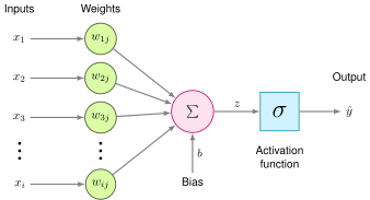](https://mlsysbook.ai/contents/core/dl_primer/0ff5c0804cf53d709bf07787bdcde4abd072ceb8.svg "Figure 10: Weighted Input Summation: Perceptrons compute a weighted sum of multiple inputs, representing feature values, and pass the result to an activation function to produce an output. each input x_i is multiplied by a corresponding weight w_{ij} before being aggregated, forming the basis for learning complex patterns from data. using this figure.")
Figure 10: **Weighted Input Summation**: Perceptrons compute a weighted sum of multiple inputs, representing feature values, and pass the result to an activation function to produce an output. each input \\(x\_i\\) is multiplied by a corresponding weight \\(w\_{ij}\\) before being aggregated, forming the basis for learning complex patterns from data. using this figure.
Visualizing these mathematical concepts, [Figure 10](https://mlsysbook.ai/contents/core/dl_primer/dl_primer.html#fig-perceptron)
illustrates the core building blocks of a perceptron, which serves as the foundation for more complex neural networks. Scaling beyond individual units, layers of perceptrons work in concert, with each layer’s output serving as the input for the subsequent layer. This hierarchical arrangement creates deep learning models capable of tackling increasingly sophisticated tasks, from image recognition to natural language processing.
Breaking down the computational mechanics, each input \\(x\_i\\) has a corresponding weight \\(w\_{ij}\\), and the perceptron simply multiplies each input by its matching weight. The intermediate output, \\(z\\), is computed as the weighted sum of inputs: \\\[ z = \\sum (x\_i \\cdot w\_{ij}) \\\]
The apparent simplicity of this mathematical expression masks its computational complexity. When scaled across millions of neurons and billions of parameters, these memory access patterns become the dominant performance bottleneck in neural network computation.
Enhancing the model’s flexibility, to this intermediate calculation, a bias term \\(b\\) is added, allowing the model to better fit the data by shifting the linear output function up or down. Thus, the intermediate linear combination computed by the perceptron including the bias becomes: \\\[ z = \\sum (x\_i \\cdot w\_{ij}) + b \\\]
This mathematical formulation directly drives the hardware requirements we discussed earlier. The summation requires accumulator units, the multiplications demand high-throughput arithmetic units, and the memory accesses necessitate high-bandwidth memory systems. Understanding this connection between mathematical operations and hardware requirements is crucial for designing efficient ML systems.
Beyond linear transformations, activation functions are critical nonlinear transformations that enable neural networks to learn complex patterns by converting linear weighted sums into nonlinear outputs. Without activation functions, multiple linear layers would collapse into a single linear transformation, severely limiting the network’s expressive power. [Figure 11](https://mlsysbook.ai/contents/core/dl_primer/dl_primer.html#fig-activation-functions)
illustrates the four most commonly used activation functions and their characteristic shapes.
[](https://mlsysbook.ai/contents/core/dl_primer/345f9cb9d7957df25080749a83ec3675b96bd560.svg "Figure 11: Common Activation Functions: Neural networks rely on nonlinear activation functions to approximate complex relationships. Each function exhibits distinct characteristics: sigmoid maps inputs to (0,1) with smooth gradients, tanh provides zero-centered outputs in (-1,1), ReLU introduces sparsity by outputting zero for negative inputs, and softmax converts logits into probability distributions. These different behaviors enable networks to learn different types of patterns and relationships.")
Figure 11: **Common Activation Functions**: Neural networks rely on nonlinear activation functions to approximate complex relationships. Each function exhibits distinct characteristics: sigmoid maps inputs to \\((0,1)\\) with smooth gradients, tanh provides zero-centered outputs in \\((-1,1)\\), ReLU introduces sparsity by outputting zero for negative inputs, and softmax converts logits into probability distributions. These different behaviors enable networks to learn different types of patterns and relationships.
The choice of activation function profoundly impacts both learning effectiveness and computational efficiency. Understanding the mathematical properties of each function is essential for designing effective neural networks. The most commonly used activation functions include:
##### Sigmoid
The sigmoid function maps any input value to a bounded range between 0 and 1: \\\[ \\sigma(x) = \\frac{1}{1 + e^{-x}} \\\]
This S-shaped curve (visible in [Figure 11](https://mlsysbook.ai/contents/core/dl_primer/dl_primer.html#fig-activation-functions)
, top-left) produces outputs that can be interpreted as probabilities, making sigmoid particularly useful for binary classification tasks. For very large positive inputs, the function approaches 1; for very large negative inputs, it approaches 0. The smooth, continuous nature of sigmoid makes it differentiable everywhere, which is necessary for gradient-based learning.
However, sigmoid has a significant limitation: for inputs with large absolute values (far from zero), the gradient becomes extremely small—a phenomenon called the **vanishing gradient problem**[18](https://mlsysbook.ai/contents/core/dl_primer/dl_primer.html#fn18)
. During backpropagation, these small gradients are multiplied together across layers, causing gradients in early layers to become exponentially tiny. This effectively prevents learning in deep networks, as weight updates become negligible.
18 **Vanishing Gradients**: When gradients become exponentially small as they propagate backward through many layers, learning effectively stops in early layers. This occurs because gradients are computed via the chain rule, multiplying derivatives from each layer. If these derivatives are consistently less than 1 (as with saturated sigmoid outputs), their product shrinks exponentially with network depth. This problem is addressed in detail in **[Chapter 8: AI Training](https://mlsysbook.ai/contents/core/training/training.html#sec-ai-training)
**.
Sigmoid outputs are not zero-centered (all outputs are positive). This asymmetry can cause inefficient weight updates during optimization, as gradients for weights connected to sigmoid units will all have the same sign.
##### Tanh
The hyperbolic tangent function addresses sigmoid’s zero-centering limitation by mapping inputs to the range \\((-1, 1)\\): \\\[ \\tanh(x) = \\frac{e^x - e^{-x}}{e^x + e^{-x}} \\\]
As shown in [Figure 11](https://mlsysbook.ai/contents/core/dl_primer/dl_primer.html#fig-activation-functions)
(top-right), tanh produces an S-shaped curve similar to sigmoid but centered at zero. Negative inputs map to negative outputs, while positive inputs map to positive outputs. This symmetry helps balance gradient flow during training, often leading to faster convergence than sigmoid.
Like sigmoid, tanh is smooth and differentiable everywhere. It still suffers from the vanishing gradient problem for inputs with large magnitudes. When the function saturates (approaches -1 or 1), gradients become very small. Despite this limitation, tanh’s zero-centered outputs make it preferable to sigmoid for hidden layers in many architectures, particularly in recurrent neural networks where maintaining balanced activations across time steps is important.
##### ReLU
The Rectified Linear Unit (ReLU) revolutionized deep learning by providing a simple solution to the vanishing gradient problem ([Nair and Hinton 2010](https://mlsysbook.ai/contents/core/dl_primer/dl_primer.html#ref-nair2010rectified)
)[19](https://mlsysbook.ai/contents/core/dl_primer/dl_primer.html#fn19)
: \\\[ \\text{ReLU}(x) = \\max(0, x) = \\begin{cases} x & \\text{if } x > 0 \\\\ 0 & \\text{if } x \\leq 0 \\end{cases} \\\]
Nair, Vinod, and Geoffrey E. Hinton. 2010. “Rectified Linear Units Improve Restricted Boltzmann Machines.” In _Proceedings of the 27th International Conference on Machine Learning (ICML-10)_, 807–14. [https://icml.cc/Conferences/2010/papers/432.pdf](https://icml.cc/Conferences/2010/papers/432.pdf)
.
19 **ReLU (Rectified Linear Unit)**: A piecewise linear activation function that outputs the input directly if positive, otherwise outputs zero. Introduced by Nair and Hinton in 2010, ReLU solved the vanishing gradient problem and became the default activation function in modern deep learning due to its computational simplicity and biological inspiration from neuron firing patterns.
[Figure 11](https://mlsysbook.ai/contents/core/dl_primer/dl_primer.html#fig-activation-functions)
(bottom-left) shows ReLU’s characteristic shape: a straight line for positive inputs and zero for negative inputs. This simplicity provides several advantages:
**Gradient Flow**: For positive inputs, ReLU’s gradient is exactly 1, allowing gradients to flow unchanged through the network. This prevents the vanishing gradient problem that plagues sigmoid and tanh in deep architectures.
**Sparsity**: By setting all negative activations to zero, ReLU introduces natural sparsity in the network. Typically, about 50% of neurons in a ReLU network output zero for any given input. This sparsity can help reduce overfitting and makes the network more interpretable.
**Computational Efficiency**: Unlike sigmoid and tanh, which require expensive exponential calculations, ReLU is computed with a simple comparison and conditional operation: `output = (input > 0) ? input : 0`. This simplicity translates to faster computation and lower energy consumption, particularly important for deployment on resource-constrained devices.
ReLU is not without drawbacks. The **dying ReLU problem** occurs when neurons become “stuck” outputting zero. If a neuron’s weights are updated such that its weighted input is consistently negative, the neuron outputs zero and contributes zero gradient during backpropagation. This neuron effectively becomes non-functional and can never recover. Careful initialization and learning rate selection help mitigate this issue.
##### Softmax
Unlike the previous activation functions that operate independently on each value, softmax considers all values simultaneously to produce a probability distribution: \\\[ \\text{softmax}(z\_i) = \\frac{e^{z\_i}}{\\sum\_{j=1}^K e^{z\_j}} \\\]
For a vector of \\(K\\) values (often called logits), softmax transforms them into \\(K\\) probabilities that sum to 1. [Figure 11](https://mlsysbook.ai/contents/core/dl_primer/dl_primer.html#fig-activation-functions)
(bottom-right) shows one component of the softmax output; in practice, softmax processes entire vectors where each element’s output depends on all input values.
Softmax is almost exclusively used in the output layer for multi-class classification problems. By converting arbitrary real-valued logits into probabilities, softmax enables the network to express confidence across multiple classes. The class with the highest probability becomes the predicted class. The exponential function ensures that larger logits receive disproportionately higher probabilities, creating clear distinctions between classes when the network is confident.
The mathematical relationship between input logits and output probabilities is differentiable, allowing gradients to flow back through softmax during training. When combined with cross-entropy loss (discussed in **[Chapter 8: AI Training](https://mlsysbook.ai/contents/core/training/training.html#sec-ai-training)
**), softmax produces particularly clean gradient expressions that guide learning effectively.
Systems Perspective: Activation Functions and Hardware
**Why ReLU Dominates in Practice**: Beyond its mathematical benefits like avoiding vanishing gradients, ReLU’s hardware efficiency explains its widespread adoption. Computing \\(\\max(0,x)\\) requires a single comparison operation, while sigmoid and tanh require computing exponentials—operations that are orders of magnitude more expensive in both time and energy. This computational simplicity means ReLU can be executed faster on any processor and consumes significantly less power, a critical consideration for battery-powered devices. The computational and hardware implications of activation functions, including performance benchmarks and implementation strategies for modern accelerators, are explored in **[Chapter 8: AI Training](https://mlsysbook.ai/contents/core/training/training.html#sec-ai-training)
**.
[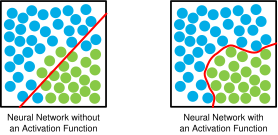](https://mlsysbook.ai/contents/core/dl_primer/55b563ec34b72c8d629e0c2c558c38331404ac76.svg "Figure 12: Non-Linear Activation: Neural networks model complex relationships by applying non-linear activation functions to weighted sums of inputs, enabling the representation of non-linear decision boundaries. These functions transform input values, creating the capacity to learn intricate patterns beyond linear combinations via the arrangement of points. Source: Medium, sachin kaushik.")
Figure 12: **Non-Linear Activation**: Neural networks model complex relationships by applying non-linear activation functions to weighted sums of inputs, enabling the representation of non-linear decision boundaries. These functions transform input values, creating the capacity to learn intricate patterns beyond linear combinations via the arrangement of points. Source: Medium, sachin kaushik.
As detailed in the activation function section above, these nonlinear transformations convert the linear input sum into a non-linear output: \\\[ \\hat{y} = \\sigma(z) \\\]
Thus, the final output of the perceptron, including the activation function, can be expressed as:
[Figure 12](https://mlsysbook.ai/contents/core/dl_primer/dl_primer.html#fig-nonlinear)
shows an example where data exhibit a nonlinear pattern that could not be adequately modeled with a linear approach, demonstrating why the nonlinear activation functions discussed earlier are essential for complex pattern recognition.
The universal approximation theorem[20](https://mlsysbook.ai/contents/core/dl_primer/dl_primer.html#fn20)
establishes that neural networks with activation functions can approximate arbitrary functions. This theoretical foundation, combined with the computational and optimization characteristics of specific activation functions like ReLU and sigmoid discussed above, explains neural networks’ practical effectiveness in complex tasks.
20 **Universal Approximation Theorem**: Proven by George Cybenko (1989) and Kurt Hornik (1991), this theorem states that neural networks with just one hidden layer containing enough neurons can approximate any continuous function to arbitrary accuracy. However, the theorem doesn’t specify how many neurons are needed (could be exponentially many) or how to find the right weights. This explains why neural networks are theoretically powerful but doesn’t guarantee practical learnability—a key distinction that drove the development of deep learning architectures and better training algorithms.
Combining the linear combination with the activation function, the complete perceptron computation is: \\\[ \\hat{y} = \\sigma\\left(\\sum (x\_i \\cdot w\_{ij}) + b\\right) \\\]
#### Layers and Connections
While a single perceptron can model simple decisions, the power of neural networks comes from combining multiple neurons into layers. A layer is a collection of neurons that process information in parallel. Each neuron in a layer operates independently on the same input but with its own set of weights and bias, allowing the layer to learn different features or patterns from the same input data.
In a typical neural network, we organize these layers hierarchically:
1. **Input Layer**: Receives the raw data features
2. **Hidden Layers**: Process and transform the data through multiple stages
3. **Output Layer**: Produces the final prediction or decision
[Figure 13](https://mlsysbook.ai/contents/core/dl_primer/dl_primer.html#fig-layers)
illustrates this layered architecture. When data flows through these layers, each successive layer transforms the representation of the data, gradually building more complex and abstract features. This hierarchical processing is what gives deep neural networks their remarkable ability to learn complex patterns.
[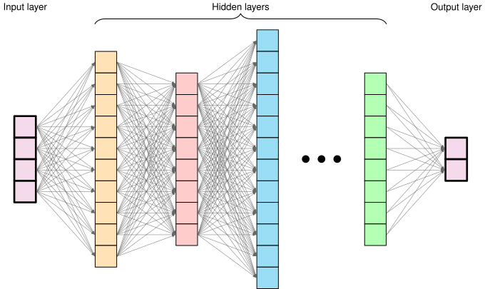](https://mlsysbook.ai/contents/core/dl_primer/d61e997272cd48b85c2f7e89f6ff4e9f33882d60.svg "Figure 13: Layered Network Architecture: Deep neural networks transform data through successive layers, enabling the extraction of increasingly complex features and patterns. each layer applies non-linear transformations to the outputs of the previous layer, ultimately mapping raw inputs to desired outputs. Source: brunellon.")
Figure 13: **Layered Network Architecture**: Deep neural networks transform data through successive layers, enabling the extraction of increasingly complex features and patterns. each layer applies non-linear transformations to the outputs of the previous layer, ultimately mapping raw inputs to desired outputs. Source: brunellon.
#### Data Flow Through Network Layers
As data flows through the network, it is transformed at each layer to extract meaningful patterns. The weighted summation and activation process we established for individual neurons scales up: each layer applies these operations in parallel across all its neurons, with outputs from one layer becoming inputs to the next. This creates a hierarchical pipeline where simple features detected in early layers combine into increasingly complex patterns in deeper layers—enabling neural networks to learn sophisticated representations from raw data.
### Parameters and Connections
The learnable parameters of neural networks consist primarily of weights and biases, which together determine how information flows through the network and how transformations are applied to input data. This section examines how these parameters are organized and structured within neural networks. We explore weight matrices that connect layers, connection patterns that define network topology, bias terms that provide flexibility in transformations, and parameter organization strategies that enable efficient computation.
#### Weight Matrices
Weights determine how strongly inputs influence neuron outputs. In larger networks, these organize into matrices for efficient computation across layers. For example, in a layer with \\(n\\) input features and \\(m\\) neurons, the weights form a matrix \\(\\mathbf{W} \\in \\mathbb{R}^{n \\times m}\\). Each column in this matrix represents the weights for a single neuron in the layer. This organization allows the network to process multiple inputs simultaneously, an essential feature for handling real-world data efficiently.
Recall that for a single neuron, we computed \\(z = \\sum\_{i=1}^n (x\_i \\cdot w\_{ij}) + b\\). When we have a layer of \\(m\\) neurons, we could compute each neuron’s output separately, but matrix operations provide a much more efficient approach. Rather than computing each neuron individually, matrix multiplication enables us to compute all \\(m\\) outputs simultaneously: \\\[ \\mathbf{z} = \\mathbf{x}^T\\mathbf{W} + \\mathbf{b} \\\]
This matrix organization is more than just mathematical convenience; it reflects how modern neural networks are implemented for efficiency. Each weight \\(w\_{ij}\\) represents the strength of the connection between input feature \\(i\\) and neuron \\(j\\) in the layer.
#### Network Connectivity Architectures
In the simplest and most common case, each neuron in a layer is connected to every neuron in the previous layer, forming what we call a “dense” or “fully-connected” layer. This pattern means that each neuron has the opportunity to learn from all available features from the previous layer. While this chapter focuses on fully-connected layers to establish foundational principles, alternative connectivity patterns (explored in **[Chapter 4: DNN Architectures](https://mlsysbook.ai/contents/core/dnn_architectures/dnn_architectures.html#sec-dnn-architectures)
**) can dramatically improve efficiency for structured data by restricting connections based on problem characteristics.
[Figure 14](https://mlsysbook.ai/contents/core/dl_primer/dl_primer.html#fig-connections)
illustrates these dense connections between layers. For a network with layers of sizes \\((n\_1, n\_2, n\_3)\\), the weight matrices would have dimensions:
* Between first and second layer: \\(\\mathbf{W}^{(1)} \\in \\mathbb{R}^{n\_1 \\times n\_2}\\)
* Between second and third layer: \\(\\mathbf{W}^{(2)} \\in \\mathbb{R}^{n\_2 \\times n\_3}\\)
[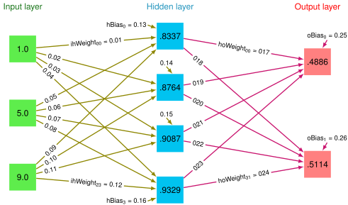](https://mlsysbook.ai/contents/core/dl_primer/dbdfb8f228253cea7198f849d0d6146436d8b878.svg "Figure 14: Fully-Connected Layers: Multilayer perceptrons (MLPs) utilize dense connections between layers, enabling each neuron to integrate information from all neurons in the preceding layer. The weight matrices defining these connections—\mathbf{W}^{(1)} \in \mathbb{R}^{n_1 \times n_2} and \mathbf{W}^{(2)} \in \mathbb{R}^{n_2 \times n_3}—determine the strength of these integrations and facilitate learning complex patterns from input data. Source: J. McCaffrey.")
Figure 14: **Fully-Connected Layers**: Multilayer perceptrons (MLPs) utilize dense connections between layers, enabling each neuron to integrate information from all neurons in the preceding layer. The weight matrices defining these connections—\\(\\mathbf{W}^{(1)} \\in \\mathbb{R}^{n\_1 \\times n\_2}\\) and \\(\\mathbf{W}^{(2)} \\in \\mathbb{R}^{n\_2 \\times n\_3}\\)—determine the strength of these integrations and facilitate learning complex patterns from input data. Source: J. McCaffrey.
#### Bias Terms
Each neuron in a layer also has an associated bias term. While weights determine the relative importance of inputs, biases allow neurons to shift their activation functions. This shifting is crucial for learning, as it gives the network flexibility to fit more complex patterns.
For a layer with \\(m\\) neurons, the bias terms form a vector \\(\\mathbf{b} \\in \\mathbb{R}^m\\). When we compute the layer’s output, this bias vector is added to the weighted sum of inputs: \\\[ \\mathbf{z} = \\mathbf{x}^T\\mathbf{W} + \\mathbf{b} \\\]
The bias terms[21](https://mlsysbook.ai/contents/core/dl_primer/dl_primer.html#fn21)
effectively allow each neuron to have a different “threshold” for activation, making the network more expressive.
21 **Bias Terms**: Constant values added to weighted inputs that allow neurons to shift their activation functions horizontally, enabling networks to model patterns that don’t pass through the origin. Without bias terms, a neuron with all-zero inputs would always produce zero output, severely limiting representational capacity. Biases typically require 1-5% of total parameters but provide crucial flexibility—for example, allowing a digit classifier to have different baseline tendencies for recognizing each digit based on frequency in training data.
#### Weight and Bias Storage Organization
The organization of weights and biases across a neural network follows a systematic pattern. For a network with \\(L\\) layers, we maintain:
* A weight matrix \\(\\mathbf{W}^{(l)}\\) for each layer \\(l\\)
* A bias vector \\(\\mathbf{b}^{(l)}\\) for each layer \\(l\\)
* Activation functions \\(f^{(l)}\\) for each layer \\(l\\)
This gives us the complete layer computation: \\\[ \\mathbf{h}^{(l)} = f^{(l)}(\\mathbf{z}^{(l)}) = f^{(l)}(\\mathbf{h}^{(l-1)T}\\mathbf{W}^{(l)} + \\mathbf{b}^{(l)}) \\\] Where \\(\\mathbf{h}^{(l)}\\) represents the layer’s output after applying the activation function.
Checkpoint: Neural Network Architecture Fundamentals
Before proceeding to network topology and training, verify your understanding of the foundational concepts we’ve covered:
**Core Concepts:**
* **Neuron Computation**: Can you write the equation for a neuron’s output, including the weighted sum, bias term, and activation function?
* **Activation Functions**: Can you explain why ReLU is computationally efficient compared to sigmoid, and why nonlinearity is essential?
* **Layer Organization**: Can you describe the three types of layers (input, hidden, output) and how they transform data sequentially?
* **Weight Matrices**: Do you understand how a weight matrix \\(\\mathbf{W}^{(l)} \\in \\mathbb{R}^{n \\times m}\\) connects a layer of \\(n\\) neurons to a layer of \\(m\\) neurons?
* **Parameter Count**: Given a network architecture (e.g., 784→128→64→10), can you calculate the total number of parameters (weights + biases)?
**Systems Implications:**
* Can you explain why neural network computation is memory-bandwidth-limited rather than compute-limited?
* Do you understand why each architectural choice (layer width, depth, connectivity) directly affects memory and computational requirements?
**Self-Test Example**: For a digit recognition network with layers 784→100→10, calculate: (1) parameters in each weight matrix, (2) total parameter count, (3) activations stored during inference for a single image.
_If any of these feel unclear, review [Section 1.4](https://mlsysbook.ai/contents/core/dl_primer/dl_primer.html#sec-dl-primer-neural-network-fundamentals-68cd)
(Neural Network Fundamentals), [Section 1.4.1.1](https://mlsysbook.ai/contents/core/dl_primer/dl_primer.html#sec-dl-primer-nonlinear-activation-functions-868a)
(Neurons and Activations), or [Section 1.4.2](https://mlsysbook.ai/contents/core/dl_primer/dl_primer.html#sec-dl-primer-parameters-connections-6c54)
(Weights and Biases) before continuing. The upcoming sections on training and optimization build directly on these foundations._
### Architecture Design
Network topology describes how individual neurons organize into layers and connect to form complete neural networks. Building intuition begins with a simple problem that became famous in AI history[22](https://mlsysbook.ai/contents/core/dl_primer/dl_primer.html#fn22)
.
22 **XOR Problem**: The exclusive-or function became famous in AI history when Marvin Minsky and Seymour Papert proved in 1969 that single-layer perceptrons could never learn it, contributing to the “AI winter” of the 1970s. XOR requires non-linear decision boundaries—something impossible with linear models. The solution requires at least one hidden layer, demonstrating why “deep” networks (with hidden layers) are essential for learning complex patterns. This simple 2-input, 1-output problem helped establish the theoretical foundation for multi-layer neural networks.
**Example:** Building Intuition: The XOR Problem
Consider a network learning the XOR function—a classic problem that requires non-linearity. With inputs \\(x\_1\\) and \\(x\_2\\) that can be 0 or 1, XOR outputs 1 when inputs differ and 0 when they’re the same.
**Network Structure**: 2 inputs → 2 hidden neurons → 1 output
**Forward Pass Example**: For inputs \\((1, 0)\\):
* Hidden neuron 1: \\(h\_1 = \\text{ReLU}(1 \\cdot w\_{11} + 0 \\cdot w\_{12} + b\_1)\\)
* Hidden neuron 2: \\(h\_2 = \\text{ReLU}(1 \\cdot w\_{21} + 0 \\cdot w\_{22} + b\_2)\\)
* Output: \\(y = \\text{sigmoid}(h\_1 \\cdot w\_{31} + h\_2 \\cdot w\_{32} + b\_3)\\)
This simple network demonstrates how hidden layers enable learning non-linear patterns—something a single layer cannot achieve.
The XOR example established the fundamental three-layer architecture, but real-world networks require systematic consideration of design constraints and computational scale[23](https://mlsysbook.ai/contents/core/dl_primer/dl_primer.html#fn23)
. Recognizing handwritten digits using the MNIST ([Lecun et al. 1998](https://mlsysbook.ai/contents/core/dl_primer/dl_primer.html#ref-lecun1998gradient)
)[24](https://mlsysbook.ai/contents/core/dl_primer/dl_primer.html#fn24)
dataset illustrates how problem structure determines network dimensions while hidden layer configuration remains a critical design decision.
23 **Computational Scale Considerations**: Network size decisions involve balancing accuracy against computational costs. A 784→1000→1000→10 MNIST network has ~1.8M parameters requiring ~7MB memory, while a 784→100→100→10 network needs only ~90K parameters and ~350KB memory. The larger network might achieve 99.5% vs 98.5% accuracy, but requires 20× more memory and computation—often an unacceptable trade-off for mobile deployment where every megabyte and millisecond matters.
Lecun, Y., L. Bottou, Y. Bengio, and P. Haffner. 1998. “Gradient-Based Learning Applied to Document Recognition.” _Proceedings of the IEEE_ 86 (11): 2278–2324. [https://doi.org/10.1109/5.726791](https://doi.org/10.1109/5.726791)
.
24 **MNIST Dataset**: Created by Yann LeCun and colleagues in 1998, MNIST (Modified National Institute of Standards and Technology) contains 70,000 images of handwritten digits—60,000 for training and 10,000 for testing. Each image is 28×28 pixels in grayscale, totaling 784 features per digit. MNIST became the “hello world” of computer vision, with error rates dropping from 12% with traditional methods in 1998 to 0.23% with modern deep learning. Despite being “solved,” MNIST remains invaluable for teaching because it’s large enough to be realistic yet small enough to train quickly on any computer.
#### Feedforward Network Architecture
Applying the three-layer architecture to MNIST reveals how data characteristics and task requirements constrain network design. As shown in [Figure 15](https://mlsysbook.ai/contents/core/dl_primer/dl_primer.html#fig-mnist-topology-1)
\\(\\text{a)}\\), a \\(28\\times 28\\) pixel grayscale image of a handwritten digit must be processed through input, hidden, and output layers to produce a classification output.
The input layer’s width is directly determined by our data format. As shown in [Figure 15](https://mlsysbook.ai/contents/core/dl_primer/dl_primer.html#fig-mnist-topology-1)
\\(\\text{b)}\\), for a \\(28\\times 28\\) pixel image, each pixel becomes an input feature, requiring 784 input neurons \\((28\\times 28 = 784)\\). We can think of this either as a 2D grid of pixels or as a flattened vector of 784 values, where each value represents the intensity of one pixel.
The output layer’s structure is determined by our task requirements. For digit classification, we use 10 output neurons, one for each possible digit (0-9). When presented with an image, the network produces a value for each output neuron, where higher values indicate greater confidence that the image represents that particular digit.
Between these fixed input and output layers, we have flexibility in designing the hidden layer topology. The choice of hidden layer structure, including the number of layers to use and their respective widths, represents one of the key design decisions in neural networks. Additional layers increase the network’s depth, allowing it to learn more abstract features through successive transformations. The width of each layer provides capacity for learning different features at each level of abstraction.
[](https://mlsysbook.ai/contents/core/dl_primer/f88a65f5a2a811f40a894ea8cfddd9ae246b2f3f.svg "Figure 15: \text{a)} A neural network topology for classifying MNIST digits, showing how a 28\times 28 pixel image is processed. The image on the left shows the original digit, with dimensions labeled. The network on the right shows how each pixel connects to the hidden layers, ultimately producing 10 outputs for digit classification. \text{b)} Alternative visualization of the MNIST network topology, showing how the 2D image is flattened into a 784-dimensional vector before being processed by the network. This representation emphasizes how spatial data is transformed into a format suitable for neural network processing.")
Figure 15: \\(\\text{a)}\\) A neural network topology for classifying MNIST digits, showing how a \\(28\\times 28\\) pixel image is processed. The image on the left shows the original digit, with dimensions labeled. The network on the right shows how each pixel connects to the hidden layers, ultimately producing 10 outputs for digit classification. \\(\\text{b)}\\) Alternative visualization of the MNIST network topology, showing how the 2D image is flattened into a 784-dimensional vector before being processed by the network. This representation emphasizes how spatial data is transformed into a format suitable for neural network processing.
These basic topological choices have significant implications for both the network’s capabilities and its computational requirements. Each additional layer or neuron increases the number of parameters that must be stored and computed during both training and inference. However, without sufficient depth or width, the network may lack the capacity to learn complex patterns in the data.
#### Design Trade-offs: Depth vs Width vs Performance
The design of neural network topology centers on three key decisions: the number of layers (depth), the size of each layer (width), and how these layers connect. Each choice affects both the network’s learning capability and its computational requirements.
Network depth determines achievable abstraction: stacked layers build increasingly complex features through successive transformations. For MNIST, shallow layers detect edges, intermediate layers combine edges into strokes, and deep layers assemble complete digit patterns. However, additional depth increases computational cost, training difficulty (vanishing gradients), and architectural complexity without guaranteed benefits.
The width of each layer, which is determined by the number of neurons it contains, controls how much information the network can process in parallel at each stage. Wider layers can learn more features simultaneously but require proportionally more parameters and computation. For instance, if a hidden layer is processing edge features in our digit recognition task, its width determines how many different edge patterns it can detect simultaneously.
A very important consideration in topology design is the total parameter count. For a network with layers of size \\((n\_1, n\_2, \\ldots, n\_L)\\), each pair of adjacent layers \\(l\\) and \\(l+1\\) requires \\(n\_l \\times n\_{l+1}\\) weight parameters, plus \\(n\_{l+1}\\) bias parameters. These parameters must be stored in memory and updated during training, making the parameter count a key constraint in practical applications.
Network design requires balancing learning capacity, computational efficiency, and training tractability. While the basic approach connects every neuron to every neuron in the next layer (fully connected), this does not always represent the most effective strategy. The fully-connected approach assumes every input element may interact with every other—yet real-world data rarely exhibits such unconstrained relationships.
Consider the MNIST example: a 28×28 image has 784 pixels, creating 306,936 possible pixel pairs (\\(\\frac{784 \\times 783}{2}\\)). A fully-connected first layer with 100 neurons learns 78,400 weights, effectively examining every possible pixel relationship. Neighboring pixels (forming edges of digits) interact more than pixels at opposite corners. Fully-connected layers spend parameters and computation learning that pixel (1,1) doesn’t interact strongly with pixel (28,28), relationships we could encode structurally. Specialized architectures (explored in **[Chapter 4: DNN Architectures](https://mlsysbook.ai/contents/core/dnn_architectures/dnn_architectures.html#sec-dnn-architectures)
**) address this inefficiency by restricting connections based on problem structure, achieving superior results with 10-100× fewer parameters by exploiting spatial locality, temporal ordering, or other domain-specific patterns.
Information flow through the network represents another important consideration. While the basic flow proceeds from input to output, some network designs include additional paths such as skip connections or residual connections. These alternative paths facilitate training and improve effectiveness at learning complex patterns by functioning as shortcuts that enable more direct information flow when needed, analogous to how the human brain combines detailed and general impressions during object recognition.
These design decisions have significant practical implications including memory usage for storing network parameters, computational costs during both training and inference, training behavior and convergence, and the network’s ability to generalize to new examples. The optimal balance of these trade-offs depends heavily on the specific problem, available computational resources, and dataset characteristics. Successful network design requires careful consideration of these factors against practical constraints.
With our understanding of network architecture established—how neurons connect into layers, how layers stack into networks, and how design choices affect computational requirements—we can now address the central question: how do these networks learn? The architecture provides the structure, but the learning process brings that structure to life by discovering the weight values that enable accurate predictions.
Systems Perspective: Architecture Shapes Deployment Feasibility
**From Design to Deployment**: Every architectural decision—number of layers, layer widths, connection patterns—directly determines memory requirements and computational cost. A network with 1 million parameters requires roughly 4MB of memory just to store weights, before considering activations during inference. As models grow deeper and wider, their memory footprint and computational demands grow quadratically, not linearly. This mathematical relationship between architecture and resource requirements explains why the same architectural patterns cannot deploy uniformly across all platforms. Systems engineering insight emerges: architectural design must consider target deployment constraints from the outset, as post-hoc compression only partially recovers from architecture-resource mismatches.
#### Layer Connectivity Design Patterns
Neural networks can be structured with different connection patterns between layers, each offering distinct advantages for learning and computation. Understanding these patterns provides insight into how networks process information and learn representations from data.
Dense connectivity represents the standard pattern where each neuron connects to every neuron in the subsequent layer. In our MNIST example, connecting our 784-dimensional input layer to a hidden layer of 100 neurons requires 78,400 weight parameters. This full connectivity enables the network to learn arbitrary relationships between inputs and outputs, but the number of parameters scales quadratically with layer width.
Sparse connectivity patterns introduce purposeful restrictions in how neurons connect between layers. Rather than maintaining all possible connections, neurons connect to only a subset of neurons in the adjacent layer. This approach draws inspiration from biological neural systems, where neurons typically form connections with a limited number of other neurons. In visual processing tasks like our MNIST example, neurons might connect only to inputs representing nearby pixels, reflecting the local nature of visual features.
As networks grow deeper, the path from input to output becomes longer, potentially complicating the learning process. Skip connections address this by adding direct paths between non-adjacent layers. These connections provide alternative routes for information flow, supplementing the standard layer-by-layer progression. In our digit recognition example, skip connections might allow later layers to reference both high-level patterns and the original pixel values directly.
These connection patterns have significant implications for both the theoretical capabilities and practical implementation of neural networks. Dense connections maximize learning flexibility at the cost of computational efficiency. Sparse connections can reduce computational requirements while potentially improving the network’s ability to learn structured patterns. Skip connections help maintain effective information flow in deeper networks.
#### Model Size and Computational Complexity
The arrangement of parameters (weights and biases) in a neural network determines both its learning capacity and computational requirements. While topology defines the network’s structure, the initialization and organization of parameters plays a crucial role in learning and performance.
Parameter count grows with network width and depth. For our MNIST example, consider a network with a 784-dimensional input layer, two hidden layers of 100 neurons each, and a 10-neuron output layer. The first layer requires 78,400 weights and 100 biases, the second layer 10,000 weights and 100 biases, and the output layer 1,000 weights and 10 biases, totaling 89,610 parameters. Each must be stored in memory and updated during learning.
Parameter initialization is critical to network behavior. Setting all parameters to zero would cause neurons in a layer to behave identically, preventing diverse feature learning. Instead, weights are typically initialized randomly, while biases often start at small constant values or even zeros. The scale of these initial values matters significantly, as values that are too large or too small can lead to poor learning dynamics.
The distribution of parameters affects information flow through layers. In digit recognition, if weights are too small, important input details might not propagate to later layers. If too large, the network might amplify noise. Biases help adjust the activation threshold of each neuron, enabling the network to learn optimal decision boundaries.
Different architectures may impose specific constraints on parameter organization. Some share weights across network regions to encode position-invariant pattern recognition. Others might restrict certain weights to zero, implementing sparse connectivity patterns.
With our understanding of network architecture, neurons, and parameters established, we can now address the fundamental question: how do these randomly initialized parameters become useful? The answer lies in the learning process that transforms a network from its initial random state into a system capable of making accurate predictions.
**Self-Check: Question 1.4**
1. Which of the following best describes the role of the activation function in a neural network?
1. To linearly combine the inputs
2. To store the weights of the network
3. To introduce non-linearity into the model
4. To initialize the biases
2. Explain why ReLU is favored over sigmoid activation functions in deep neural networks.
3. In a neural network designed for MNIST digit recognition, what is the primary function of the hidden layers?
1. To store the input data
2. To extract and transform features from the input data
3. To perform the final classification
4. To normalize the input data
4. Deep neural networks can suffer from training difficulties where information flow becomes less effective in earlier layers, commonly called the \_\_\_\_ problem.
5. In a production system, how might you decide between using a fully-connected layer and a sparse connectivity pattern?
[See Answers →](https://mlsysbook.ai/contents/core/dl_primer/dl_primer.html#quiz-answer-sec-dl-primer-neural-network-fundamentals-68cd)
Learning Process
----------------
Neural networks learn to perform tasks through a process of training on examples. This process transforms the network from its initial state, where weights are randomly initialized as we just discussed, to a trained state where these same weights encode meaningful patterns from the training data. Understanding this process is essential to both the theoretical foundations and practical implementations of deep learning models.
### Supervised Learning from Labeled Examples
Building on our architectural foundation, the core principle of neural network training is supervised learning from labeled examples. Consider our MNIST digit recognition task: we have a dataset of 60,000 training images, each a \\(28\\times 28\\) pixel grayscale image paired with its correct digit label. The network must learn the relationship between these images and their corresponding digits through an iterative process of prediction and weight adjustment. Ensuring the quality and integrity of training data is essential to model success, as covered in **[Chapter 6: Data Engineering](https://mlsysbook.ai/contents/core/data_engineering/data_engineering.html#sec-data-engineering)
**.
This relationship between inputs and outputs drives the training methodology. Training operates as a loop, where each iteration involves processing a subset of training examples called a batch[25](https://mlsysbook.ai/contents/core/dl_primer/dl_primer.html#fn25)
. For each batch, the network performs several key operations:
25 **Batch Processing**: Processing multiple examples simultaneously, typically 32-256 samples per batch. Larger batches provide more stable gradient estimates and better utilize parallel hardware but require more memory. The optimal batch size depends on available GPU memory and the specific model architecture.
* Forward computation through the network layers to generate predictions
* Evaluation of prediction accuracy using a loss function
* Computation of weight adjustments based on prediction errors
* Update of network weights to improve future predictions
Formalizing this iterative approach, this process can be expressed mathematically. Given an input image \\(x\\) and its true label \\(y\\), the network computes its prediction: \\\[ \\hat{y} = f(x; \\theta) \\\] where \\(f\\) represents the neural network function and \\(\\theta\\) represents all trainable parameters (weights and biases, which we discussed earlier). The network’s error is measured by a loss function \\(L\\): \\\[ \\text{loss} = L(\\hat{y}, y) \\\]
This quantification of prediction quality becomes the foundation for learning. This error measurement drives the adjustment of network parameters through a process called “backpropagation,” which we will examine in detail later.
Scaling beyond individual examples, in practice, training operates on batches of examples rather than individual inputs. For the MNIST dataset, each training iteration might process, for example, 32, 64, or 128 images simultaneously. This batch processing serves two purposes: it enables efficient use of modern computing hardware through parallel processing, and it provides more stable parameter updates by averaging errors across multiple examples.
This batch-based approach creates both computational efficiency and training stability. The training cycle continues until the network achieves sufficient accuracy or reaches a predetermined number of iterations. Throughout this process, the loss function serves as a guide, with its minimization indicating improved network performance. Establishing proper metrics and evaluation protocols is crucial for assessing training effectiveness, as discussed in **[Chapter 12: Benchmarking AI](https://mlsysbook.ai/contents/core/benchmarking/benchmarking.html#sec-benchmarking-ai)
**.
### Forward Pass Computation
Forward propagation, as illustrated in [Figure 16](https://mlsysbook.ai/contents/core/dl_primer/dl_primer.html#fig-forward-propagation)
, is the core computational process in a neural network, where input data flows through the network’s layers to generate predictions. Understanding this process is important as it underlies both network inference and training. We examine how forward propagation works using our MNIST digit recognition example.
[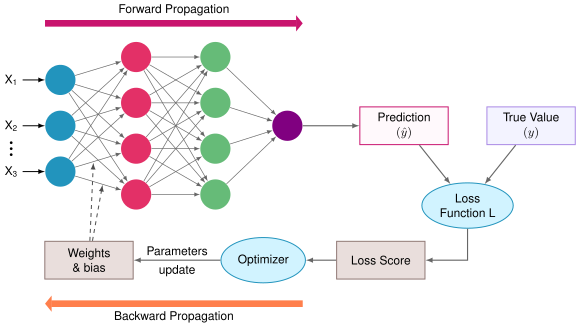](https://mlsysbook.ai/contents/core/dl_primer/7cb579a47d65631ddbcd793f25264af43e33ef55.svg "Figure 16: Forward Propagation Process: Neural networks transform input data into predictions by sequentially applying weighted sums and activation functions across interconnected layers, enabling complex pattern recognition. This layered computation forms the basis for both making inferences and updating model parameters during training.")
Figure 16: **Forward Propagation Process**: Neural networks transform input data into predictions by sequentially applying weighted sums and activation functions across interconnected layers, enabling complex pattern recognition. This layered computation forms the basis for both making inferences and updating model parameters during training.
When an image of a handwritten digit enters our network, it undergoes a series of transformations through the layers. Each transformation combines the weighted inputs with learned patterns to progressively extract relevant features. In our MNIST example, a \\(28\\times 28\\) pixel image is processed through multiple layers to ultimately produce probabilities for each possible digit (0-9).
The process begins with the input layer, where each pixel’s grayscale value becomes an input feature. For MNIST, this means 784 input values \\((28\\times 28 = 784)\\), each normalized between 0 and 1. These values then propagate forward through the hidden layers, where each neuron combines its inputs according to its learned weights and applies a nonlinear activation function.
From a computational perspective, each forward pass through our MNIST network (784→128→64→10) requires substantial matrix operations. The first layer alone performs nearly 100,000 multiply-accumulate operations per sample. When processing multiple samples in a batch, these operations multiply accordingly, requiring careful management of memory bandwidth and computational resources. Specialized hardware like GPUs can execute these operations efficiently through parallel processing.
#### Individual Layer Processing
The forward computation through a neural network proceeds systematically, with each layer transforming its inputs into increasingly abstract representations. In our MNIST network, this transformation process occurs in distinct stages.
At each layer, the computation involves two key steps: a linear transformation of inputs followed by a nonlinear activation. The linear transformation applies the same weighted sum operation we’ve seen before, but now using notation that tracks which layer we’re in: \\\[ \\mathbf{Z}^{(l)} = \\mathbf{W}^{(l)}\\mathbf{A}^{(l-1)} + \\mathbf{b}^{(l)} \\\]
Here, \\(\\mathbf{W}^{(l)}\\) represents the weight matrix for layer \\(l\\), \\(\\mathbf{A}^{(l-1)}\\) contains the activations from the previous layer (the outputs after applying activation functions), and \\(\\mathbf{b}^{(l)}\\) is the bias vector. The superscript \\((l)\\) keeps track of which layer each parameter belongs to.
Following this linear transformation, each layer applies a nonlinear activation function \\(f\\): \\\[ \\mathbf{A}^{(l)} = f(\\mathbf{Z}^{(l)}) \\\]
This process repeats at each layer, creating a chain of transformations:
Input → Linear Transform → Activation → Linear Transform → Activation → … → Output
In our MNIST example, the pixel values first undergo a transformation by the first hidden layer’s weights, converting the 784-dimensional input into an intermediate representation. Each subsequent layer further transforms this representation, ultimately producing a 10-dimensional output vector representing the network’s confidence in each possible digit.
#### Matrix Multiplication Formulation
The complete forward propagation process can be expressed as a composition of functions, each representing a layer’s transformation. Formalizing this mathematically builds on the MNIST example.
For a network with \\(L\\) layers, we can express the full forward computation as: \\\[ \\mathbf{A}^{(L)} = f^{(L)}\\Big(\\mathbf{W}^{(L)}f^{(L-1)}\\Big(\\mathbf{W}^{(L-1)}\\cdots\\big(f^{(1)}(\\mathbf{W}^{(1)}\\mathbf{X} + \\mathbf{b}^{(1)})\\big)\\cdots + \\mathbf{b}^{(L-1)}\\Big) + \\mathbf{b}^{(L)}\\Big) \\\]
While this nested expression captures the complete process, we typically compute it step by step:
1. First layer: \\\[ \\mathbf{Z}^{(1)} = \\mathbf{W}^{(1)}\\mathbf{X} + \\mathbf{b}^{(1)} \\\] \\\[ \\mathbf{A}^{(1)} = f^{(1)}(\\mathbf{Z}^{(1)}) \\\]
2. Hidden layers \\((l = 2,\\ldots, L-1)\\): \\\[ \\mathbf{Z}^{(l)} = \\mathbf{W}^{(l)}\\mathbf{A}^{(l-1)} + \\mathbf{b}^{(l)} \\\] \\\[ \\mathbf{A}^{(l)} = f^{(l)}(\\mathbf{Z}^{(l)}) \\\]
3. Output layer: \\\[ \\mathbf{Z}^{(L)} = \\mathbf{W}^{(L)}\\mathbf{A}^{(L-1)} + \\mathbf{b}^{(L)} \\\] \\\[ \\mathbf{A}^{(L)} = f^{(L)}(\\mathbf{Z}^{(L)}) \\\]
In our MNIST example, if we have a batch of \\(B\\) images, the dimensions of these operations are:
* Input \\(\\mathbf{X}\\): \\(B \\times 784\\)
* First layer weights \\(\\mathbf{W}^{(1)}\\): \\(n\_1\\times 784\\)
* Hidden layer weights \\(\\mathbf{W}^{(l)}\\): \\(n\_l\\times n\_{l-1}\\)
* Output layer weights \\(\\mathbf{W}^{(L)}\\): \\(10 \\times n\_{L-1}\\)
#### Step-by-Step Computation Sequence
Understanding how these mathematical operations translate into actual computation requires examining the forward propagation process for a batch of MNIST images. This process illustrates how data transforms from raw pixel values to digit predictions.
Consider a batch of 32 images entering our network. Each image starts as a \\(28\\times 28\\) grid of pixel values, which we flatten into a 784-dimensional vector. For the entire batch, this gives us an input matrix \\(\\mathbf{X}\\) of size \\(32\\times 784\\), where each row represents one image. The values are typically normalized to lie between 0 and 1.
The transformation at each layer proceeds as follows:
* **Input Layer Processing**: The network takes our input matrix \\(\\mathbf{X}\\) \\((32\\times 784)\\) and transforms it using the first layer’s weights. If our first hidden layer has 128 neurons, \\(\\mathbf{W}^{(1)}\\) is a \\(784\\times 128\\) matrix. The resulting computation \\(\\mathbf{X}\\mathbf{W}^{(1)}\\) produces a \\(32\\times 128\\) matrix.
* **Hidden Layer Transformations**: Each element in this matrix then has its corresponding bias added and passes through an activation function. For example, with a ReLU activation, any negative values become zero while positive values remain unchanged. This nonlinear transformation enables the network to learn complex patterns in the data.
* **Output Generation**: The final layer transforms its inputs into a \\(32\\times 10\\) matrix, where each row contains 10 values corresponding to the network’s confidence scores for each possible digit. Often, these scores are converted to probabilities using a softmax function: \\\[ P(\\text{digit } j) = \\frac{e^{z\_j}}{\\sum\_{k=1}^{10} e^{z\_k}} \\\]
For each image in the batch, this produces a probability distribution over the possible digits. The digit with the highest probability represents the network’s prediction.
#### Implementation and Optimization Considerations
The implementation of forward propagation requires careful attention to several practical aspects that affect both computational efficiency and memory usage. These considerations become particularly important when processing large batches of data or working with deep networks.
Memory management plays an important role during forward propagation. Each layer’s activations must be stored for potential use in the backward pass during training. For our MNIST example with a batch size of 32, if we have three hidden layers of sizes 128, 256, and 128, the activation storage requirements are:
* First hidden layer: \\(32\\times 128 = 4,096\\) values
* Second hidden layer: \\(32\\times 256 = 8,192\\) values
* Third hidden layer: \\(32\\times 128 = 4,096\\) values
* Output layer: \\(32\\times 10 = 320\\) values
This produces a total of 16,704 values that must be maintained in memory for each batch during training. The memory requirements scale linearly with batch size and become substantial for larger networks.
Batch processing introduces important trade-offs. Larger batches enable more efficient matrix operations and better hardware utilization but require more memory. For example, doubling the batch size to 64 would double the memory requirements for activations. This relationship between batch size, memory usage, and computational efficiency guides the choice of batch size in practice.
The organization of computations also affects performance. Matrix operations can be optimized through careful memory layout and specialized libraries. The choice of activation functions affects both the network’s learning capabilities and computational efficiency, as some functions (like ReLU) require less computation than others (like tanh or sigmoid).
The computational characteristics of neural networks favor parallel processing architectures. While traditional CPUs can execute these operations, GPUs designed for parallel computation can achieve substantial speedups—often 10-100× faster for matrix operations. Specialized AI accelerators achieve even better efficiency through techniques like reduced precision arithmetic, specialized memory architectures, and dataflow optimizations tailored for neural network computation patterns.
Energy consumption also varies significantly across hardware platforms. CPUs offer flexibility but consume more energy per operation. GPUs provide high throughput at higher power consumption. Specialized edge accelerators optimize for energy efficiency, achieving the same computations with orders of magnitude less power—a critical consideration for mobile and embedded deployments. This energy disparity stems from the fundamental memory hierarchy challenges where data movement dominates computation costs.
These considerations form the foundation for understanding the system requirements of neural networks, which we will explore in more detail in **[Chapter 4: DNN Architectures](https://mlsysbook.ai/contents/core/dnn_architectures/dnn_architectures.html#sec-dnn-architectures)
**.
Now that we understand how neural networks process inputs to generate predictions through forward propagation, a critical question emerges: how do we determine if these predictions are good? The answer lies in loss functions, which provide the mathematical framework for measuring prediction quality.
### Loss Functions
Neural networks learn by measuring and minimizing their prediction errors. Loss functions provide the algorithmic structure for quantifying these errors, serving as the essential feedback mechanism that guides the learning process. Through loss functions, we can convert the abstract goal of “making good predictions” into a concrete optimization problem.
To understand the role of loss functions, let’s continue with our MNIST digit recognition example. When the network processes a handwritten digit image, it outputs ten numbers representing its confidence in each possible digit (0-9). The loss function measures how far these predictions deviate from the true answer. For instance, if an image displays a “7”, the network should exhibit high confidence for digit “7” and low confidence for all other digits. The loss function penalizes the network when its prediction deviates from this target.
Consider a concrete example: if the network sees an image of “7” and outputs confidences: \\\[ \\mathtt{\[0.1, 0.1, 0.1, 0.0, 0.0, 0.0, 0.2, 0.3, 0.1, 0.1\]} \\\]
The highest confidence (0.3) is assigned to digit “7”, but this confidence is quite low, indicating uncertainty in the prediction. A good loss function would produce a high loss value here, signaling that the network needs significant improvement. Conversely, if the network outputs: \\\[ \\mathtt{\[0.0, 0.0, 0.0, 0.0, 0.0, 0.0, 0.0, 0.9, 0.0, 0.1\]} \\\]
The loss function should produce a lower value, as this prediction is much closer to ideal. This illustrates how loss functions guide network improvement by providing feedback on prediction quality.
#### Error Measurement Fundamentals
A loss function measures how far the network’s predictions are from the correct answers. This difference is expressed as a single number: a lower loss means the predictions are more accurate, while a higher loss indicates the network needs improvement. During training, the loss function guides the network by helping it adjust its weights to make better predictions. For example, in recognizing handwritten digits, the loss will penalize predictions that assign low confidence to the correct digit.
Mathematically, a loss function \\(L\\) takes two inputs: the network’s predictions \\(\\hat{y}\\) and the true values \\(y\\). For a single training example in our MNIST task: \\\[ L(\\hat{y}, y) = \\text{measure of discrepancy between prediction and truth} \\\]
When training with batches of data, we typically compute the average loss across all examples in the batch: \\\[ L\_{\\text{batch}} = \\frac{1}{B}\\sum\_{i=1}^B L(\\hat{y}\_i, y\_i) \\\] where \\(B\\) is the batch size and \\((\\hat{y}\_i, y\_i)\\) represents the prediction and truth for the \\(i\\)\-th example.
The choice of loss function depends on the type of task. For our MNIST classification problem, we need a loss function that can:
1. Handle probability distributions over multiple classes
2. Provide meaningful gradients for learning
3. Penalize wrong predictions effectively
4. Scale well with batch processing
#### Cross-Entropy and Classification Loss Functions
For classification tasks like MNIST digit recognition, “cross-entropy” ([Shannon 1948](https://mlsysbook.ai/contents/core/dl_primer/dl_primer.html#ref-shannon1948mathematical)
)[26](https://mlsysbook.ai/contents/core/dl_primer/dl_primer.html#fn26)
loss has emerged as the standard choice. This loss function is particularly well-suited for comparing predicted probability distributions with true class labels.
Shannon, C. E. 1948. “A Mathematical Theory of Communication.” _Bell System Technical Journal_ 27 (3): 379–423. [https://doi.org/10.1002/j.1538-7305.1948.tb01338.x](https://doi.org/10.1002/j.1538-7305.1948.tb01338.x)
.
26 **Cross-Entropy Loss**: Derived from information theory by Claude Shannon in 1948, cross-entropy measures the “surprise” when predicting incorrectly. If a model is 99% confident about the wrong answer, the loss is much higher than being 60% confident about the wrong answer. This mathematical property encourages the model to be both accurate and calibrated (confident when right, uncertain when unsure). Cross-entropy works perfectly with softmax outputs and provides strong gradients even when predictions are very wrong, making it ideal for classification tasks.
For a single digit image, our network outputs a probability distribution over the ten possible digits. We represent the true label as a one-hot vector where all entries are 0 except for a 1 at the correct digit’s position. For instance, if the true digit is “7”, the label would be: \\\[ y = \\big\[0, 0, 0, 0, 0, 0, 0, 1, 0, 0\\big\] \\\]
The cross-entropy loss for this example is: \\\[ L(\\hat{y}, y) = -\\sum\_{j=1}^{10} y\_j \\log(\\hat{y}\_j) \\\] where \\(\\hat{y}\_j\\) represents the network’s predicted probability for digit j. Given our one-hot encoding, this simplifies to: \\\[ L(\\hat{y}, y) = -\\log(\\hat{y}\_c) \\\] where \\(c\\) is the index of the correct class. This means the loss depends only on the predicted probability for the correct digit—the network is penalized based on how confident it is in the right answer.
For example, if our network predicts the following probabilities for an image of “7”:
Predicted: [0.1, 0.0, 0.0, 0.0, 0.0, 0.0, 0.0, 0.8, 0.0, 0.1]
True: [0, 0, 0, 0, 0, 0, 0, 1, 0, 0]
The loss would be \\(-\\log(0.8)\\), which is approximately 0.223. If the network were more confident and predicted 0.9 for the correct digit, the loss would decrease to approximately 0.105.
#### Batch Loss Calculation Methods
The practical computation of loss involves considerations for both numerical stability and batch processing. When working with batches of data, we compute the average loss across all examples in the batch.
For a batch of B examples, the cross-entropy loss becomes: \\\[ L\_{\\text{batch}} = -\\frac{1}{B}\\sum\_{i=1}^B \\sum\_{j=1}^{10} y\_{ij} \\log(\\hat{y}\_{ij}) \\\]
Computing this loss efficiently requires careful consideration of numerical precision. Taking the logarithm of very small probabilities can lead to numerical instability. Consider a case where our network predicts a probability of 0.0001 for the correct class. Computing \\(\\log(0.0001)\\) directly might cause underflow or result in imprecise values.
To address this, we typically implement the loss computation with two key modifications:
1. Add a small epsilon to prevent taking log of zero: \\\[ L = -\\log(\\hat{y} + \\epsilon) \\\]
2. Apply the log-sum-exp trick for numerical stability: \\\[ \\text{softmax}(z\_i) = \\frac{\\exp\\big(z\_i - \\max(z)\\big)}{\\sum\_j \\exp\\big(z\_j - \\max(z)\\big)} \\\]
For our MNIST example with a batch size of 32, this means:
* Processing 32 sets of 10 probabilities
* Computing 32 individual loss values
* Averaging these values to produce the final batch loss
#### Impact on Learning Dynamics
Understanding how loss functions influence training helps explain key implementation decisions in deep learning models.
During each training iteration, the loss value serves multiple purposes:
1. Performance Metric: It quantifies current network accuracy
2. Optimization Target: Its gradients guide weight updates
3. Convergence Signal: Its trend indicates training progress
For our MNIST classifier, monitoring the loss during training reveals the network’s learning trajectory. A typical pattern might show:
* Initial high loss (\\(\\sim 2.3\\), equivalent to random guessing among 10 classes)
* Rapid decrease in early training iterations
* Gradual improvement as the network fine-tunes its predictions
* Eventually stabilizing at a lower loss (\\(\\sim 0.1\\), indicating confident correct predictions)
The loss function’s gradients with respect to the network’s outputs provide the initial error signal that drives backpropagation. For cross-entropy loss, these gradients have a particularly simple form: the difference between predicted and true probabilities. This mathematical property makes cross-entropy loss especially suitable for classification tasks, as it provides strong gradients even when predictions are very wrong.
The choice of loss function also influences other training decisions:
* Learning rate selection (larger loss gradients might require smaller learning rates)
* Batch size (loss averaging across batches affects gradient stability)
* Optimization algorithm behavior
* Convergence criteria
Once we have quantified the network’s prediction errors through loss functions, the next critical step is determining how to adjust the network’s weights to reduce these errors. This brings us to backward propagation, the mechanism that enables neural networks to learn from their mistakes.
### Gradient Computation and Backpropagation
**Definition:** Backpropagation
**_Backpropagation_** is an algorithm that efficiently computes _gradients_ of a neural network’s _loss function_ with respect to all parameters by systematically applying the _chain rule_ backward through network layers.
Backward propagation, often called backpropagation, is the algorithmic cornerstone of neural network training that enables systematic weight adjustment through gradient-based optimization. While loss functions tell us how wrong our predictions are, backpropagation tells us exactly how to fix them.
To build intuition for this complex process, consider the “credit assignment” problem through a factory assembly line analogy. Imagine a car factory where vehicles pass through multiple stations: Station A installs the frame, Station B adds the engine, Station C attaches the wheels, and Station D performs final assembly. When quality inspectors at the end of the line find a defective car, they face a critical question: which station contributed most to the problem, and how should each station adjust its process?
The solution works backward from the defect. The inspector first examines the final assembly (Station D) and determines how its work affected the quality issue. Station D then looks at what it received from Station C and calculates how much of the problem came from the wheels versus its own assembly work. This feedback flows backward: Station C examines the engine from Station B, and Station B reviews the frame from Station A. Each station receives an “adjustment signal” proportional to how much its work contributed to the defect. If Station B’s engine mounting was the primary cause, it receives a strong signal to change its process, while stations that performed correctly receive smaller or no adjustment signals.
Backpropagation solves this credit assignment problem in neural networks systematically. The output layer (like Station D) receives the most direct feedback about what went wrong. It calculates how its inputs from the previous layer contributed to the error and sends specific adjustment signals backward through the network. Each layer receives guidance proportional to its contribution to the prediction error and adjusts its weights accordingly. This process ensures that every layer learns from the mistake, with the most responsible connections making the largest adjustments.
In neural networks, each layer acts like a station on the assembly line, and backpropagation determines how much each connection contributed to the final prediction error. This systematic approach to learning from mistakes forms the foundation of how neural networks improve through experience.
This section presents the complete optimization framework, from gradient computation through practical training implementation.
#### Backpropagation Algorithm Steps
While forward propagation computes predictions, backward propagation determines how to adjust the network’s weights to improve these predictions. To understand this process, consider our MNIST example where the network predicts a “3” for an image of “7”. Backward propagation provides a systematic way to adjust weights throughout the network to make this mistake less likely in the future by calculating how each weight contributed to the error.
The process begins at the network’s output, where we compare predicted digit probabilities with the true label. This error then flows backward through the network, with each layer’s weights receiving an update signal based on their contribution to the final prediction. The computation follows the chain rule of calculus, breaking down the complex relationship between weights and final error into manageable steps.
The mathematical foundations of backpropagation provide the theoretical basis for training neural networks, but practical implementation requires sophisticated software frameworks. Modern frameworks like PyTorch and TensorFlow implement automatic differentiation systems that handle gradient computation automatically, eliminating the need for manual derivative implementation. The systems engineering aspects of these frameworks, including computation graphs and optimization strategies, are covered comprehensively in **[Chapter 7: AI Frameworks](https://mlsysbook.ai/contents/core/frameworks/frameworks.html#sec-ai-frameworks)
**.
#### Error Signal Propagation
The flow of gradients through a neural network follows a path opposite to the forward propagation. Starting from the loss at the output layer, gradients propagate backwards, computing how each layer, and ultimately each weight, influenced the final prediction error.
In our MNIST example, consider what happens when the network misclassifies a “7” as a “3”. The loss function generates an initial error signal at the output layer, essentially indicating that the probability for “7” should increase while the probability for “3” should decrease. This error signal then propagates backward through the network layers.
For a network with L layers, the gradient flow can be expressed mathematically. At each layer l, we compute how the layer’s output affected the final loss: \\\[ \\frac{\\partial L}{\\partial \\mathbf{A}^{(l)}} = \\frac{\\partial L}{\\partial \\mathbf{A}^{(l+1)}} \\frac{\\partial \\mathbf{A}^{(l+1)}}{\\partial \\mathbf{A}^{(l)}} \\\]
This computation cascades backward through the network, with each layer’s gradients depending on the gradients computed in the layer previous to it. The process reveals how each layer’s transformation contributed to the final prediction error. For instance, if certain weights in an early layer strongly influenced a misclassification, they will receive larger gradient values, indicating a need for more substantial adjustment.
This process faces challenges in deep networks. As gradients flow backward through many layers, they can either vanish or explode. When gradients are repeatedly multiplied through many layers, they can become exponentially small, particularly with sigmoid or tanh activation functions. This causes early layers to learn very slowly or not at all, as they receive negligible updates. Conversely, if gradient values are consistently greater than 1, they can grow exponentially, leading to unstable training and destructive weight updates.
#### Derivative Calculation Process
The actual computation of gradients involves calculating several partial derivatives at each layer. For each layer, we need to determine how changes in weights, biases, and activations affect the final loss. These computations follow directly from the chain rule of calculus but must be implemented efficiently for practical neural network training.
At each layer \\(l\\), we compute three main gradient components:
1. Weight Gradients: \\\[ \\frac{\\partial L}{\\partial \\mathbf{W}^{(l)}} = \\frac{\\partial L}{\\partial \\mathbf{Z}^{(l)}} {\\mathbf{A}^{(l-1)}}^T \\\]
2. Bias Gradients: \\\[ \\frac{\\partial L}{\\partial \\mathbf{b}^{(l)}} = \\frac{\\partial L}{\\partial \\mathbf{Z}^{(l)}} \\\]
3. Input Gradients (for propagating to previous layer): \\\[ \\frac{\\partial L}{\\partial \\mathbf{A}^{(l-1)}} = {\\mathbf{W}^{(l)}}^T \\frac{\\partial L}{\\partial \\mathbf{Z}^{(l)}} \\\]
In our MNIST example, consider the final layer where the network outputs digit probabilities. If the network predicted \\(\[0.1, 0.2, 0.5,\\ldots, 0.05\]\\) for an image of “7”, the gradient computation would:
1. Start with the error in these probabilities
2. Compute how weight adjustments would affect this error
3. Propagate these gradients backward to help adjust earlier layer weights
These mathematical formulations precisely describe gradient computation, but the systems breakthrough lies in how frameworks automatically implement these calculations. Consider a simple operation like matrix multiplication followed by ReLU activation: `output = torch.relu(input @ weight)`. The mathematical gradient involves computing the derivative of ReLU (0 for negative inputs, 1 for positive) and applying the chain rule for matrix multiplication. The framework handles this automatically by:
1. Recording the operation in a computation graph during forward pass
2. Storing necessary intermediate values (pre-ReLU activations for gradient computation)
3. Automatically generating the backward pass function for each operation
4. Optimizing memory usage and computation order across the entire graph
This automation transforms gradient computation from a manual, error-prone process requiring deep mathematical expertise into a reliable system capability that enables rapid experimentation and deployment. The framework ensures correctness while optimizing for computational efficiency, memory usage, and hardware utilization.
#### Computational Implementation Details
The practical implementation of backward propagation requires careful consideration of computational resources and memory management. These implementation details significantly impact training efficiency and scalability.
Memory requirements during backward propagation stem from two main sources. First, we need to store the intermediate activations from the forward pass, as these are required for computing gradients. For our MNIST network with a batch size of 32, each layer’s activations must be maintained:
* Input layer: \\(32\\times 784\\) values (~100KB using 32-bit numbers)
* Hidden layer 1: \\(32\\times 512\\) values (~64KB)
* Hidden layer 2: \\(32\\times 256\\) values (~32KB)
* Output layer: \\(32\\times 10\\) values (~1.3KB)
Second, we must store gradients for each parameter during backward propagation. For our example network with approximately 500,000 parameters, this requires several megabytes of memory for gradients. Advanced optimizers like Adam[27](https://mlsysbook.ai/contents/core/dl_primer/dl_primer.html#fn27)
require additional memory to store momentum terms, roughly doubling the gradient storage requirements.
27 **Adam Optimizer**: Introduced by Diederik Kingma and Jimmy Ba in 2014, Adam (Adaptive Moment Estimation) combines the benefits of two other optimizers: AdaGrad’s adaptive learning rates and RMSprop’s exponential moving averages. Adam maintains separate learning rates for each parameter and adapts them based on first and second moments of gradients. It requires 2× memory overhead (storing momentum and velocity for each parameter) but typically converges faster than basic SGD. Adam became the default optimizer for most deep learning applications due to its robustness across different problems and minimal hyperparameter tuning requirements.
The memory bandwidth requirements scale with model size and batch size. Each training step requires loading all parameters, storing gradients, and accessing activations—creating substantial memory traffic. For modest networks like our MNIST example, this traffic remains manageable within typical memory system capabilities. However, as models grow larger, memory bandwidth can become a significant bottleneck, with the largest models requiring specialized high-bandwidth memory systems to maintain training efficiency.
Second, we need storage for the gradients themselves. For each layer, we must maintain gradients of similar dimensions to the weights and biases. Taking our previous example of a network with hidden layers of size 128, 256, and 128, this means storing:
* First layer gradients: \\(784\\times 128\\) values
* Second layer gradients: \\(128\\times 256\\) values
* Third layer gradients: \\(256\\times 128\\) values
* Output layer gradients: \\(128\\times 10\\) values
The computational pattern of backward propagation follows a specific sequence:
1. Compute gradients at current layer
2. Update stored gradients
3. Propagate error signal to previous layer
4. Repeat until input layer is reached
For batch processing, these computations are performed simultaneously across all examples in the batch, enabling efficient use of matrix operations and parallel processing capabilities.
Modern frameworks handle these computations through sophisticated autograd engines. When you call `loss.backward()` in PyTorch, the framework automatically manages memory allocation, operation scheduling, and gradient accumulation across the computation graph. The system tracks which tensors require gradients, optimizes memory usage through gradient checkpointing when needed, and schedules operations to maximize hardware utilization. This automated management allows practitioners to focus on model design rather than the intricate details of gradient computation implementation.
### Weight Update and Optimization
Training neural networks requires systematic adjustment of weights and biases to minimize prediction errors through an iterative optimization process. Building on the computational foundations established in our biological-to-artificial translation, this section explores the core mechanisms of neural network optimization, from gradient-based parameter updates to practical training implementations.
#### Parameter Update Algorithms
**Definition:** Gradient Descent
**_Gradient Descent_** is an iterative optimization algorithm that minimizes a _loss function_ by repeatedly adjusting parameters in the direction of _steepest descent_, calculated from the _gradient_ with respect to those parameters.
The optimization process adjusts network weights through gradient descent[28](https://mlsysbook.ai/contents/core/dl_primer/dl_primer.html#fn28)
, a systematic method that implements the learning principles derived from our biological neural network analysis. This iterative process calculates how each weight contributes to the error and updates parameters to reduce loss, gradually refining the network’s predictive ability.
28 **Gradient Descent**: Think of gradient descent as finding the bottom of a valley while blindfolded—you feel the slope under your feet and take steps downhill. Mathematically, the gradient points in the direction of steepest increase, so we move in the opposite direction to minimize our loss function. The name comes from the Latin “gradus” (step) and was first formalized by Cauchy in 1847 for solving systems of equations, though the modern machine learning version was developed much later.
The fundamental update rule combines backpropagation’s gradient computation with parameter adjustment: \\\[ \\theta\_{\\text{new}} = \\theta\_{\\text{old}} - \\alpha \\nabla\_{\\theta}L \\\] where \\(\\theta\\) represents any network parameter (weights or biases), \\(\\alpha\\) is the learning rate, and \\(\\nabla\_{\\theta}L\\) is the gradient computed through backpropagation.
For our MNIST example, this means adjusting weights to improve digit classification accuracy. If the network frequently confuses “7”s with “1”s, gradient descent will modify weights to better distinguish between these digits. The learning rate \\(\\alpha\\)[29](https://mlsysbook.ai/contents/core/dl_primer/dl_primer.html#fn29)
controls adjustment magnitude—too large values cause overshooting optimal parameters, while too small values result in slow convergence.
29 **Learning Rate**: Often called the most important hyperparameter in deep learning, the learning rate determines the step size in optimization. Think of it like the gas pedal on a car—too much acceleration and you’ll crash past your destination, too little and you’ll never get there. Typical values range from 0.1 to 0.0001, and getting this right can mean the difference between a model that learns in hours versus one that never converges.
Frankle, Jonathan, and Michael Carbin. 2019. “The Lottery Ticket Hypothesis: Finding Sparse, Trainable Neural Networks.” In _International Conference on Learning Representations_. [https://openreview.net/forum?id=rJl-b3RcF7](https://openreview.net/forum?id=rJl-b3RcF7)
.
Neyshabur, Behnam, Srinadh Bhojanapalli, David McAllester, and Nati Srebro. 2017. “Exploring Generalization in Deep Learning.” _Advances in Neural Information Processing Systems_ 30. [https://proceedings.neurips.cc/paper/2017/hash/10ce03a1ed01077e3e289f3e53c72813-Abstract.html](https://proceedings.neurips.cc/paper/2017/hash/10ce03a1ed01077e3e289f3e53c72813-Abstract.html)
.
Nakkiran, Preetum, Gal Kaplun, Yamini Bansal, Tristan Yang, Boaz Barak, and Ilya Sutskever. 2019. “Deep Double Descent: Where Bigger Models and More Data Hurt.” _arXiv Preprint arXiv:1912.02292_, December. [http://arxiv.org/abs/1912.02292v1](http://arxiv.org/abs/1912.02292v1)
.
Despite neural network loss landscapes being highly non-convex with multiple local minima, gradient descent reliably finds effective solutions in practice. The theoretical reasons—involving concepts like the lottery ticket hypothesis ([Frankle and Carbin 2019](https://mlsysbook.ai/contents/core/dl_primer/dl_primer.html#ref-frankle2018lottery)
), implicit bias ([Neyshabur et al. 2017](https://mlsysbook.ai/contents/core/dl_primer/dl_primer.html#ref-neyshabur2017exploring)
), and overparameterization benefits ([Nakkiran et al. 2019](https://mlsysbook.ai/contents/core/dl_primer/dl_primer.html#ref-nakkiran2019deep)
)—remain active research areas. For practical ML systems engineering, the key insight is that gradient descent with appropriate learning rates, initialization, and regularization consistently trains neural networks to high performance.
#### Mini-Batch Gradient Updates
Neural networks typically process multiple examples simultaneously during training, an approach known as mini-batch gradient descent. Rather than updating weights after each individual image, we compute the average gradient over a batch of examples before performing the update.
For a batch of size \\(B\\), the loss gradient becomes: \\\[ \\nabla\_{\\theta}L\_{\\text{batch}} = \\frac{1}{B}\\sum\_{i=1}^B \\nabla\_{\\theta}L\_i \\\]
In our MNIST training, with a typical batch size of 32, this means:
1. Process 32 images through forward propagation
2. Compute loss for all 32 predictions
3. Average the gradients across all 32 examples
4. Update weights using this averaged gradient
Systems Perspective: Batch Size and Hardware Utilization
**The Batch Size Trade-off**: Larger batches improve hardware efficiency because matrix operations can process multiple examples with similar computational cost to processing one. However, each example in the batch requires memory to store its activations, creating a fundamental trade-off: larger batches use hardware more efficiently but demand more memory. Available memory thus becomes a hard constraint on batch size, which in turn affects how efficiently the hardware can be utilized. This relationship between algorithm design (batch size) and hardware capability (memory) exemplifies why ML systems engineering requires thinking about both simultaneously.
#### Iterative Learning Process
The complete training process combines forward propagation, backward propagation, and weight updates into a systematic training loop. This loop repeats until the network achieves satisfactory performance or reaches a predetermined number of iterations.
A single pass through the entire training dataset is called an epoch[30](https://mlsysbook.ai/contents/core/dl_primer/dl_primer.html#fn30)
. For MNIST, with 60,000 training images and a batch size of 32, each epoch consists of 1,875 batch iterations. The training loop structure is:
30 **Epoch**: From the Greek word “epoche” meaning “fixed point in time,” an epoch represents one complete cycle through all training data. Deep learning models typically require 10-200 epochs to converge, depending on dataset size and complexity. Modern large language models like GPT-3 train on only 1 epoch over massive datasets (300 billion tokens), while smaller models might train for 100+ epochs on limited data. The term was borrowed from astronomy, where it marks a specific moment for measuring celestial positions—fitting for the iterative refinement process of neural network training.
1. For each epoch:
* Shuffle training data to prevent learning order-dependent patterns
* For each batch:
* Perform forward propagation
* Compute loss
* Execute backward propagation
* Update weights using gradient descent
* Evaluate network performance
During training, we monitor several key metrics:
* Training loss: average loss over recent batches
* Validation accuracy: performance on held-out test data
* Learning progress: how quickly the network improves
For our digit recognition task, we might observe the network’s accuracy improve from 10% (random guessing) to over 95% through multiple epochs of training.
#### Convergence and Stability Considerations
The successful implementation of neural network training requires attention to several key practical aspects that significantly impact learning effectiveness. These considerations bridge the gap between theoretical understanding and practical implementation.
**Definition:** Overfitting
**_Overfitting_** occurs when a machine learning model learns patterns specific to the _training data_ that fail to generalize to _unseen data_, resulting in high training accuracy but poor test performance.
Learning rate selection is perhaps the most critical parameter affecting training. For our MNIST network, the choice of learning rate dramatically influences the training dynamics. A large learning rate of 0.1 might cause unstable training where the loss oscillates or explodes as weight updates overshoot optimal values. Conversely, a very small learning rate of 0.0001 might result in extremely slow convergence, requiring many more epochs to achieve good performance. A moderate learning rate of 0.01 often provides a good balance between training speed and stability, allowing the network to make steady progress while maintaining stable learning.
Convergence monitoring provides crucial feedback during the training process. As training progresses, we typically observe the loss value stabilizing around a particular value, indicating the network is approaching a local optimum. The validation accuracy often plateaus as well, suggesting the network has extracted most of the learnable patterns from the data. The gap between training and validation performance offers insights into whether the network is overfitting or generalizing well to new examples. The operational aspects of monitoring models in production environments, including detecting model degradation and performance drift, are comprehensively covered in **[Chapter 13: ML Operations](https://mlsysbook.ai/contents/core/ops/ops.html#sec-ml-operations)
**.
Resource requirements become increasingly important as we scale neural network training. The memory footprint must accommodate both model parameters and the intermediate computations needed for backpropagation. Computation scales linearly with batch size, affecting training speed and hardware utilization. Modern training often leverages GPU acceleration, making efficient use of parallel computing capabilities crucial for practical implementation.
Training neural networks also presents several challenges. Overfitting occurs when the network becomes too specialized to the training data, performing well on seen examples but poorly on new ones. Gradient instability can manifest as either vanishing or exploding gradients, making learning difficult. The interplay between batch size, available memory, and computational resources often requires careful balancing to achieve efficient training while working within hardware constraints.
Checkpoint: Neural Network Learning Process
You’ve now covered the complete training cycle—the mathematical machinery that enables neural networks to learn from data. Before moving to inference and deployment, verify your understanding:
**Forward Propagation:**
* Can you trace data flow through a network, computing activations layer-by-layer using \\(\\mathbf{Z}^{(l)} = \\mathbf{W}^{(l)}\\mathbf{A}^{(l-1)} + \\mathbf{b}^{(l)}\\) and \\(\\mathbf{A}^{(l)} = f(\\mathbf{Z}^{(l)})\\)?
* Do you understand why we must store intermediate activations during forward propagation?
**Loss Functions:**
* Can you explain what cross-entropy loss measures and why \\(L = -\\log(\\hat{y}\_c)\\) penalizes low confidence in the correct class?
* Do you understand why we average loss across a batch rather than computing it per-example?
**Backward Propagation:**
* Can you explain conceptually how gradients flow backward through the network using the chain rule?
* Do you understand why we need stored activations from the forward pass to compute gradients?
* Can you describe the vanishing gradient problem and why it affects deep networks?
**Optimization:**
* Can you write the gradient descent update rule: \\(\\theta\_{\\text{new}} = \\theta\_{\\text{old}} - \\alpha \\nabla\_{\\theta}L\\)?
* Do you understand the trade-offs between batch size (memory vs. throughput vs. gradient stability)?
* Can you explain what an epoch represents and why we typically train for multiple epochs?
**The Complete Training Loop:**
* Can you describe the four-step cycle: forward pass → compute loss → backward pass → update weights?
* Do you understand why training requires significantly more memory than inference?
**Self-Test**: For our MNIST network (784→128→64→10), trace what happens during one training iteration with batch size 32: What matrices multiply? What gets stored? What memory is required? What gradients are computed?
_If any concepts feel unclear, review [Section 1.5.2](https://mlsysbook.ai/contents/core/dl_primer/dl_primer.html#sec-dl-primer-forward-pass-computation-a837)
(Forward Propagation), [Section 1.5.3](https://mlsysbook.ai/contents/core/dl_primer/dl_primer.html#sec-dl-primer-loss-functions-d892)
(Loss Functions), [Section 1.5.4](https://mlsysbook.ai/contents/core/dl_primer/dl_primer.html#sec-dl-primer-gradient-computation-backpropagation-e26a)
(Backward Propagation), or [Section 1.5.5](https://mlsysbook.ai/contents/core/dl_primer/dl_primer.html#sec-dl-primer-weight-update-optimization-20af)
(Optimization Process). These mechanisms form the foundation for understanding the training-vs-inference distinction we explore next._
**Self-Check: Question 1.5**
1. What is the primary purpose of using batch processing in neural network training?
1. To increase the speed of individual predictions
2. To enhance the accuracy of the model
3. To reduce the overall memory usage
4. To improve the stability of gradient estimates
2. True or False: Larger batch sizes always lead to better model performance.
3. Explain how forward propagation contributes to computational efficiency in neural networks.
4. The general process of adjusting network parameters based on prediction errors is known as \_\_\_\_. This process is crucial for improving model accuracy through iterative updates.
5. In a production system, what considerations would you take into account when choosing the batch size for training a neural network?
[See Answers →](https://mlsysbook.ai/contents/core/dl_primer/dl_primer.html#quiz-answer-sec-dl-primer-learning-process-38a0)
Inference Pipeline
------------------
Having explored the training process in detail, we now turn to the operational phase of neural networks. Neural networks serve two distinct purposes: learning from data during training and making predictions during inference. While we’ve explored how networks learn through forward propagation, backward propagation, and weight updates, the prediction phase operates differently. During inference, networks use their learned parameters to transform inputs into outputs without the need for learning mechanisms. This simpler computational process still requires careful consideration of how data flows through the network and how system resources are utilized. Understanding the prediction phase is crucial as it represents how neural networks are actually deployed to solve real-world problems, from classifying images to generating text predictions.
### Production Deployment and Prediction Pipeline
The operational deployment of neural networks centers on inference, which is the process of using trained models to make predictions on new data. Unlike training, which requires iterative parameter updates and extensive computational resources, inference represents the production workload that delivers value in deployed systems. Understanding the fundamental differences between these two phases proves essential for designing efficient ML systems, as each phase imposes distinct requirements on hardware, memory, and software architecture. This section examines the core characteristics of inference, beginning with a systematic comparison to training before exploring the computational pipeline that transforms inputs into predictions.
This phase transition introduces an important constraint regarding model adaptability that significantly impacts system design. While trained models demonstrate generalization capabilities across unseen inputs through learned statistical patterns, the learned parameters remain fixed throughout deployment. Once training concludes, the model applies its learned probability distributions without modification. When the operational data distribution diverges from training distributions, the model continues executing its fixed computational pathways regardless of this shift. Consider an autonomous vehicle perception system: if construction zone frequency increases substantially or novel vehicle configurations appear in deployment, the model’s responses reflect the statistical patterns learned during training rather than adapting to the evolved operational context. The capacity for adaptation in ML systems emerges not from runtime model modification but from systematic retraining with updated data, a deliberate engineering process detailed in **[Chapter 8: AI Training](https://mlsysbook.ai/contents/core/training/training.html#sec-ai-training)
**.
#### Operational Phase Differences
Neural network operation divides into two fundamentally distinct phases that impose markedly different computational requirements and system constraints. Training requires both forward and backward passes through the network to compute gradients and update weights, while inference involves only forward pass computation. This architectural simplification means that each layer performs only one set of operations during inference, transforming inputs to outputs using learned weights without tracking intermediate values for gradient computation, as illustrated in [Figure 17](https://mlsysbook.ai/contents/core/dl_primer/dl_primer.html#fig-training-vs-inference)
.
These computational differences manifest directly in hardware requirements and deployment strategies. Training clusters typically employ high-memory GPUs[31](https://mlsysbook.ai/contents/core/dl_primer/dl_primer.html#fn31)
with substantial cooling infrastructure. Inference deployments prioritize latency and energy efficiency across diverse platforms: mobile devices utilize low-power neural processors (typically 2-4W), edge servers deploy specialized inference accelerators[32](https://mlsysbook.ai/contents/core/dl_primer/dl_primer.html#fn32)
, and cloud services employ inference-optimized instances with reduced numerical precision for increased throughput[33](https://mlsysbook.ai/contents/core/dl_primer/dl_primer.html#fn33)
. Production inference systems serving millions of requests daily require sophisticated infrastructure including load balancing, auto-scaling, and failover mechanisms typically unnecessary in training environments.
31 **Training GPU Requirements**: Modern training GPUs like the NVIDIA A100 or H100 provide 80GB of high-bandwidth memory and consume 300-700W during operation. This high memory capacity accommodates large models and training batches, while the power consumption reflects the intensive parallel computation required for gradient calculations across millions of parameters.
32 **Edge AI Accelerators**: Specialized processors like Google’s Edge TPU optimize for inference efficiency, achieving 4 TOPS/W (trillion operations per second per watt of power)—roughly 10-100× more energy-efficient than general-purpose processors for neural network operations. This efficiency enables deployment on battery-powered devices like smartphones and IoT sensors.
33 **Inference Numerical Precision**: Inference systems often use reduced precision arithmetic—16-bit or 8-bit numbers instead of 32-bit—to increase throughput while maintaining accuracy. This precision reduction exploits the fact that trained models are more robust to numerical approximation than the training process itself. Using 8-bit integers can provide 4× throughput improvement compared to 32-bit floating-point operations.
[](https://mlsysbook.ai/contents/core/dl_primer/7e8bda543a5a49b5d988117429e33161846be324.svg "Figure 17: Inference vs. Training Flow: During inference, neural networks utilize learned weights for forward pass computation only, simplifying the data flow and reducing computational cost compared to training, which requires both forward and backward passes for weight updates. This streamlined process enables efficient deployment of trained models for real-time predictions.")
Figure 17: **Inference vs. Training Flow**: During inference, neural networks utilize learned weights for forward pass computation only, simplifying the data flow and reducing computational cost compared to training, which requires both forward and backward passes for weight updates. This streamlined process enables efficient deployment of trained models for real-time predictions.
Parameter freezing represents another major distinction between training and inference phases. During training, weights and biases continuously update to minimize the loss function. In inference, these parameters remain fixed, acting as static transformations learned from the training data. This freezing of parameters not only simplifies computation but also enables optimizations impossible during training, such as weight quantization or pruning.
The structural difference between training loops and inference passes significantly impacts system design. Training operates in an iterative loop, processing multiple batches of data repeatedly across many epochs to refine the network’s parameters. Inference, in contrast, typically processes each input just once, generating predictions in a single forward pass. This shift from iterative refinement to single-pass prediction influences how we architect systems for deployment.
These structural differences create substantially different memory and computation requirements between training and inference. Training demands considerable memory to store intermediate activations for backpropagation, gradients for weight updates, and optimization states. Inference eliminates these memory-intensive requirements, needing only enough memory to store the model parameters and compute a single forward pass. This reduction in memory footprint, coupled with simpler computation patterns, enables inference to run efficiently on a broader range of devices, from powerful servers to resource-constrained edge devices.
In general, the training phase requires more computational resources and memory for learning, while inference is streamlined for efficient prediction. [Table 5](https://mlsysbook.ai/contents/core/dl_primer/dl_primer.html#tbl-train-vs-inference)
summarizes the key differences between training and inference.
Table 5: **Training vs. Inference**: Neural networks transition from a computationally intensive training phase—requiring both forward and backward passes with updated parameters—to an efficient inference phase using fixed parameters and solely forward passes. This distinction enables deployment on resource-constrained devices by minimizing memory requirements and computational load during prediction.
| | | |
| --- | --- | --- |
| **Computation Flow** | Forward and backward passes, gradient computation | Forward pass only, direct input to output |
| **Parameters** | Continuously updated weights and biases | Fixed/frozen weights and biases |
| **Processing Pattern** | Iterative loops over multiple epochs | Single pass through the network |
| **Memory Requirements** | High – stores activations, gradients, optimizer state | Lower– stores only model parameters and current input |
| **Computational Needs** | Heavy – gradient updates, backpropagation | Lighter – matrix multiplication only |
| **Hardware Requirements** | GPUs/specialized hardware for efficient training | Can run on simpler devices, including mobile/edge |
This stark contrast between training and inference phases highlights why system architectures often differ significantly between development and deployment environments. While training requires substantial computational resources and specialized hardware, inference can be optimized for efficiency and deployed across a broader range of devices.
Training and inference enable different architectural optimizations. Training requires high-precision arithmetic and backward pass computation, driving specialized hardware adoption with flexible compute units. Inference allows for various efficiency optimizations and specialized architectures that take advantage of the simpler computational flow. These differences explain why specialized inference processors can achieve much higher energy efficiency compared to general-purpose training hardware.
Memory usage patterns also differ dramatically: training stores all activations for backpropagation (requiring 2-3x more memory), while inference can discard activations immediately after use.
#### End-to-End Prediction Workflow
The implementation of neural networks in practical applications requires a complete processing pipeline that extends beyond the network itself. This pipeline, which is illustrated in [Figure 18](https://mlsysbook.ai/contents/core/dl_primer/dl_primer.html#fig-inference-pipeline)
transforms raw inputs into meaningful outputs through a series of distinct stages, each essential for the system’s operation. Understanding this complete pipeline provides critical insights into the design and deployment of deep learning systems.
[](https://mlsysbook.ai/contents/core/dl_primer/c0cfb4a2d13a1b77c336e555ebbfc4976109151d.svg "Figure 18: Inference Pipeline: Machine learning systems transform raw inputs into final outputs through a series of sequential stages—preprocessing, neural network computation, and post-processing—each critical for accurate prediction and deployment. This pipeline emphasizes the distinction between model architecture and the complete system required for real-world application.")
Figure 18: **Inference Pipeline**: Machine learning systems transform raw inputs into final outputs through a series of sequential stages—preprocessing, neural network computation, and post-processing—each critical for accurate prediction and deployment. This pipeline emphasizes the distinction between model architecture and the complete system required for real-world application.
The key thing to notice from the figure is that deep learning systems operate as hybrid architectures that combine conventional computing operations with neural network computations. The neural network component, focused on learned transformations through matrix operations, represents just one element within a broader computational framework. This framework encompasses both the preparation of input data and the interpretation of network outputs, processes that rely primarily on traditional computing methods.
Consider how data flows through the pipeline in [Figure 18](https://mlsysbook.ai/contents/core/dl_primer/dl_primer.html#fig-inference-pipeline)
:
1. Raw inputs arrive in their original form, which might be images, text, sensor readings, or other data types
2. Pre-processing transforms these inputs into a format suitable for neural network consumption
3. The neural network performs its learned transformations
4. Raw outputs emerge from the network, often in numerical form
5. Post-processing converts these outputs into meaningful, actionable results
This pipeline structure reveals several key characteristics of deep learning systems. The neural network, despite its computational sophistication, functions as a component within a larger system. Performance bottlenecks may arise at any stage of the pipeline, not exclusively within the neural network computation. System optimization must therefore consider the entire pipeline rather than focusing solely on the neural network’s operation.
The hybrid nature of this architecture has significant implications for system implementation. While neural network computations may benefit from specialized hardware accelerators, pre- and post-processing operations typically execute on conventional processors. This distribution of computation across heterogeneous hardware resources represents a fundamental consideration in system design.
### Data Preprocessing and Normalization
The pre-processing stage transforms raw inputs into a format suitable for neural network computation. While often overlooked in theoretical discussions, this stage forms a critical bridge between real-world data and neural network operations. Consider our MNIST digit recognition example: before a handwritten digit image can be processed by the neural network we designed earlier, it must undergo several transformations. Raw images of handwritten digits arrive in various formats, sizes, and pixel value ranges. For instance, in [Figure 19](https://mlsysbook.ai/contents/core/dl_primer/dl_primer.html#fig-handwritten)
, we see that the digits are all of different sizes, and even the number 6 is written differently by the same person.
[](https://mlsysbook.ai/contents/core/dl_primer/images/png/handwritten_digits.png "Figure 19: Handwritten Digit Variability: Real-world data exhibits substantial variation in style, size, and orientation, necessitating robust pre-processing techniques for reliable machine learning performance. These images exemplify the challenges of digit recognition, where even seemingly simple inputs require normalization and feature extraction before they can be effectively processed by a neural network. Source: o. augereau.")
Figure 19: **Handwritten Digit Variability**: Real-world data exhibits substantial variation in style, size, and orientation, necessitating robust pre-processing techniques for reliable machine learning performance. These images exemplify the challenges of digit recognition, where even seemingly simple inputs require normalization and feature extraction before they can be effectively processed by a neural network. Source: o. augereau.
The pre-processing stage standardizes these inputs through conventional computing operations:
* Image scaling to the required \\(28\\times 28\\) pixel dimensions, camera images are usually large(r).
* Pixel value normalization from \\(\[0,255\]\\) to \\(\[0,1\]\\), most cameras generate colored images.
* Flattening the 2D image array into a 784-dimensional vector, preparing it for the neural network.
* Basic validation to ensure data integrity, making sure the network predicted correctly.
What distinguishes pre-processing from neural network computation is its reliance on traditional computing operations rather than learned transformations. While the neural network learns to recognize digits through training, pre-processing operations remain fixed, deterministic transformations. This distinction has important system implications: pre-processing operates on conventional CPUs rather than specialized neural network hardware, and its performance characteristics follow traditional computing patterns.
The effectiveness of pre-processing directly impacts system performance. Poor normalization can lead to reduced accuracy, inconsistent scaling can introduce artifacts, and inefficient implementation can create bottlenecks. Understanding these implications helps in designing robust deep learning systems that perform well in real-world conditions.
### Forward Pass Computation Pipeline
The inference phase represents the operational state of a neural network, where learned parameters are used to transform inputs into predictions. Unlike the training phase we discussed earlier, inference focuses solely on forward computation with fixed parameters.
#### Model Loading and Setup
Before processing any inputs, the neural network must be properly initialized for inference. This initialization phase involves loading the model parameters learned during training into memory. For our MNIST digit recognition network, this means loading specific weight matrices and bias vectors for each layer. The exact memory requirements for our architecture are:
* Input to first hidden layer:
* Weight matrix: \\(784\\times 100 = 78,400\\) parameters
* Bias vector: 100 parameters
* First to second hidden layer:
* Weight matrix: \\(100\\times 100 = 10,000\\) parameters
* Bias vector: 100 parameters
* Second hidden layer to output:
* Weight matrix: \\(100\\times 10 = 1,000\\) parameters
* Bias vector: 10 parameters
This architecture’s complete parameter requirements are detailed in the Resource Requirements section below. For processing a single image, this means allocating space for:
* First hidden layer activations: 100 values
* Second hidden layer activations: 100 values
* Output layer activations: 10 values
This memory allocation pattern differs significantly from training, where additional memory was needed for gradients, optimizer states, and backpropagation computations.
Real-world inference deployments employ various memory optimization techniques to reduce resource requirements while maintaining acceptable accuracy. Systems may combine multiple requests together to better utilize hardware capabilities while meeting response time requirements. For resource-constrained deployments, various model compression approaches help models fit within available memory while preserving functionality.
#### Inference Forward Pass Execution
During inference, data propagates through the network’s layers using the initialized parameters. This forward propagation process, while similar in structure to its training counterpart, operates with different computational constraints and optimizations. The computation follows a deterministic path from input to output, transforming the data at each layer using learned parameters.
For our MNIST digit recognition network, consider the precise computations at each layer. The network processes a pre-processed image represented as a 784-dimensional vector through successive transformations:
1. First Hidden Layer Computation:
* Input transformation: 784 inputs combine with 78,400 weights through matrix multiplication
* Linear computation: \\(\\mathbf{z}^{(1)} = \\mathbf{x}\\mathbf{W}^{(1)} + \\mathbf{b}^{(1)}\\)
* Activation: \\(\\mathbf{a}^{(1)} = \\text{ReLU}(\\mathbf{z}^{(1)})\\)
* Output: 100-dimensional activation vector
2. Second Hidden Layer Computation:
* Input transformation: 100 values combine with 10,000 weights
* Linear computation: \\(\\mathbf{z}^{(2)} = \\mathbf{a}^{(1)}\\mathbf{W}^{(2)} + \\mathbf{b}^{(2)}\\)
* Activation: \\(\\mathbf{a}^{(2)} = \\text{ReLU}(\\mathbf{z}^{(2)})\\)
* Output: 100-dimensional activation vector
3. Output Layer Computation:
* Final transformation: 100 values combine with 1,000 weights
* Linear computation: \\(\\mathbf{z}^{(3)} = \\mathbf{a}^{(2)}\\mathbf{W}^{(3)} + \\mathbf{b}^{(3)}\\)
* Activation: \\(\\mathbf{a}^{(3)} = \\text{softmax}(\\mathbf{z}^{(3)})\\)
* Output: 10 probability values
[Table 6](https://mlsysbook.ai/contents/core/dl_primer/dl_primer.html#tbl-forward-pass)
shows how these computations, while mathematically identical to training-time forward propagation, show important operational differences:
Table 6: **Forward Pass Optimization**: During inference, neural networks prioritize computational efficiency by retaining only current layer activations and releasing intermediate states, unlike training where complete activation history is maintained for backpropagation. This optimization streamlines output generation by focusing resources on immediate computations rather than gradient preparation.
| | | |
| --- | --- | --- |
| **Activation Storage** | Maintains complete activation history for backpropagation | Retains only current layer activations |
| **Memory Pattern** | Preserves intermediate states throughout forward pass | Releases memory after layer computation completes |
| **Computational Flow** | Structured for gradient computation preparation | Optimized for direct output generation |
| **Resource Profile** | Higher memory requirements for training operations | Minimized memory footprint for efficient execution |
This streamlined computation pattern enables efficient inference while maintaining the network’s learned capabilities. The reduction in memory requirements and simplified computational flow make inference particularly suitable for deployment in resource-constrained environments, such as Mobile ML and Tiny ML.
#### Memory and Computational Resources
Neural networks consume computational resources differently during inference compared to training. During inference, resource utilization focuses primarily on efficient forward pass computation and minimal memory overhead. Examining the specific requirements for the MNIST digit recognition network reveals:
Memory requirements during inference can be precisely quantified:
1. Static Memory (Model Parameters):
* Layer 1: 78,400 weights + 100 biases
* Layer 2: 10,000 weights + 100 biases
* Layer 3: 1,000 weights + 10 biases
* Total: 89,610 parameters (\\(\\approx 358.44\\) KB at 32-bit floating point precision[34](https://mlsysbook.ai/contents/core/dl_primer/dl_primer.html#fn34)
)
34 **32-bit Floating Point Precision**: Also called “single precision” or FP32, this IEEE 754 standard uses 32 bits to represent real numbers: 1 bit for sign, 8 bits for exponent, and 23 bits for mantissa. While neural network training typically requires FP32 precision to maintain gradient stability, inference often works with FP16 (half precision) or even INT8 (8-bit integers), reducing memory usage by 2× to 4×. Modern AI chips like Google’s TPU v4 support “bfloat16” (brain floating point), a custom 16-bit format that maintains FP32’s range while halving memory requirements.
2. Dynamic Memory (Activations):
* Layer 1 output: 100 values
* Layer 2 output: 100 values
* Layer 3 output: 10 values
* Total: 210 values (\\(\\approx 0.84\\) KB at 32-bit floating point precision)
Computational requirements follow a fixed pattern for each input:
* First layer: 78,400 multiply-adds
* Second layer: 10,000 multiply-adds
* Output layer: 1,000 multiply-adds
* Total: 89,400 multiply-add operations per inference
This resource profile stands in stark contrast to training requirements, where additional memory for gradients and computational overhead for backpropagation significantly increase resource demands. The predictable, streamlined nature of inference computations enables various optimization opportunities and efficient hardware utilization.
#### Performance Enhancement Techniques
The fixed nature of inference computation presents several opportunities for optimization that are not available during training. Once a neural network’s parameters are frozen, the predictable pattern of computation allows for systematic improvements in both memory usage and computational efficiency.
Batch size selection represents a key trade-off in inference optimization. During training, large batches were necessary for stable gradient computation, but inference offers more flexibility. Processing single inputs minimizes latency, making it ideal for real-time applications where immediate responses are crucial. However, batch processing can significantly improve throughput by better utilizing parallel computing capabilities, particularly on GPUs. For our MNIST network, consider the memory implications: processing a single image requires storing 210 activation values, while a batch of 32 images requires 6,720 activation values but can process images up to 32 times faster on parallel hardware.
Memory management during inference can be significantly more efficient than during training. Since intermediate values are only needed for forward computation, memory buffers can be carefully managed and reused. The activation values from each layer need only exist until the next layer’s computation is complete. This enables in-place operations where possible, reducing the total memory footprint. The fixed nature of inference allows for precise memory alignment and access patterns optimized for the underlying hardware architecture.
Hardware-specific optimizations become particularly important during inference. On CPUs, computations can be organized to maximize cache utilization and take advantage of parallel processing capabilities where the same operation is applied to multiple data elements simultaneously. GPU deployments benefit from optimized matrix multiplication routines and efficient memory transfer patterns. These optimizations extend beyond pure computational efficiency, as they can significantly impact power consumption and hardware utilization, critical factors in real-world deployments.
The predictable nature of inference also enables optimizations like reduced numerical precision. While training typically requires full floating-point precision to maintain stable learning, inference can often operate with reduced precision while maintaining acceptable accuracy. For our MNIST network, such optimizations could significantly reduce the memory footprint with corresponding improvements in computational efficiency.
These optimization principles, while illustrated through our simple MNIST feedforward network, represent only the foundation of neural network optimization. More sophisticated architectures introduce additional considerations and opportunities, including specialized designs for spatial data processing, sequential computation, and attention-based computation patterns. These architectural variations and their optimizations are explored in **[Chapter 4: DNN Architectures](https://mlsysbook.ai/contents/core/dnn_architectures/dnn_architectures.html#sec-dnn-architectures)
**, **[Chapter 10: Model Optimizations](https://mlsysbook.ai/contents/core/optimizations/optimizations.html#sec-model-optimizations)
**, and **[Chapter 9: Efficient AI](https://mlsysbook.ai/contents/core/efficient_ai/efficient_ai.html#sec-efficient-ai)
**.
### Output Interpretation and Decision Making
The transformation of neural network outputs into actionable predictions requires a return to traditional computing paradigms. Just as pre-processing bridges real-world data to neural computation, post-processing bridges neural outputs back to conventional computing systems. This completes the hybrid computing pipeline we examined earlier, where neural and traditional computing operations work in concert to solve real-world problems.
The complexity of post-processing extends beyond simple mathematical transformations. Real-world systems must handle uncertainty, validate outputs, and integrate with larger computing systems. In our MNIST example, a digit recognition system might require not just the most likely digit, but also confidence measures to determine when human intervention is needed. This introduces additional computational steps: confidence thresholds, secondary prediction checks, and error handling logic, all of which are implemented in traditional computing frameworks.
The computational requirements of post-processing differ significantly from neural network inference. While inference benefits from parallel processing and specialized hardware, post-processing typically runs on conventional CPUs and follows sequential logic patterns. This return to traditional computing brings both advantages and constraints. Operations are more flexible and easier to modify than neural computations, but they may become bottlenecks if not carefully implemented. For instance, computing softmax probabilities for a batch of predictions requires different optimization strategies than the matrix multiplications of neural network layers.
System integration considerations often dominate post-processing design. Output formats must match downstream system requirements, error handling must align with broader system protocols, and performance must meet system-level constraints. In a complete mail sorting system, the post-processing stage must not only identify digits but also format these predictions for the sorting machinery, handle uncertainty cases appropriately, and maintain processing speeds that match physical mail flow rates.
This return to traditional computing paradigms completes the hybrid nature of deep learning systems. Just as pre-processing prepared real-world data for neural computation, post-processing adapts neural outputs for real-world use. Understanding this hybrid nature, the interplay between neural and traditional computing, is essential for designing and implementing effective deep learning systems.
We’ve now covered the complete lifecycle of neural networks: from architectural design through training dynamics to inference deployment. Each concept—neurons, layers, forward propagation, backpropagation, loss functions, optimization—represents a piece of the puzzle. But how do these pieces fit together in practice? The following checkpoint helps you verify your understanding of how these components integrate into complete systems, after which we’ll examine a historical case study that brings all these principles to life in a real-world deployment.
Checkpoint: Complete Neural Network System
Before examining how these concepts integrate in a real-world deployment, verify your understanding of the complete neural network lifecycle:
**Integration Across Phases:**
* Can you trace how architectural decisions (layer sizes, activation functions) impact both training dynamics and inference performance?
* Do you understand how parameter counts translate to memory requirements across training and inference phases?
* Can you explain why the same network requires 2-3× more memory during training than inference?
**Training to Deployment:**
* Can you trace the complete lifecycle: architecture design → training loop → trained model → inference deployment?
* Do you understand how training metrics (loss, gradients) differ from deployment metrics (latency, throughput)?
* Can you explain when human intervention is needed (confidence thresholds, validation, monitoring)?
**Inference and Deployment:**
* Can you explain the key differences between training and inference (computation flow, memory requirements, parameter updates)?
* Do you understand the complete inference pipeline: preprocessing → neural network → post-processing?
* Can you explain why inference is simpler and more efficient than training?
**Systems Integration:**
* Do you understand why neural networks require specialized hardware (memory bandwidth constraints, parallel computation)?
* Can you explain why ML systems combine traditional computing (preprocessing, post-processing) with neural computation?
* Do you understand the trade-offs between batch size, memory, and throughput?
**End-to-End Flow:**
* Can you trace a single input (e.g., MNIST digit image) through the complete system: raw input → preprocessing → forward propagation through layers → output probabilities → post-processing → final prediction?
* Do you understand the distinction between what happens once (loading trained weights) versus per-input (forward propagation)?
**Self-Test**: For an MNIST digit classifier (784→128→64→10) deployed in production: (1) Explain why training this model requires ~12GB GPU memory while inference needs only ~400MB. (2) Trace a single digit image from camera capture through preprocessing, inference, and post-processing to final prediction. (3) Identify where bottlenecks might occur in a real-time system processing 100 images/second. (4) Describe how you would monitor for model degradation in production.
_The following case study demonstrates how these concepts integrate in a production system deployed at massive scale. Watch for how architectural choices, training strategies, and deployment constraints combine to create a working ML system._
**Self-Check: Question 1.6**
1. Which of the following best describes a key difference between training and inference in neural networks?
1. Inference operates in iterative loops over multiple epochs, similar to training.
2. Inference requires more memory than training due to the need to store gradients.
3. Training uses fixed parameters, whereas inference updates parameters continuously.
4. Training requires both forward and backward passes, while inference requires only forward passes.
2. Explain why inference in neural networks is typically more efficient than training, in terms of computational and memory requirements.
3. Order the following stages of the inference pipeline: (1) Pre-processing, (2) Neural Network Computation, (3) Post-processing.
4. In a production system, which optimization technique is commonly used during inference to improve throughput without significantly affecting accuracy?
1. Using 32-bit floating point precision for all computations.
2. Increasing the number of epochs for inference.
3. Batch processing of inputs to utilize parallel computing capabilities.
4. Storing all intermediate activations for future reference.
[See Answers →](https://mlsysbook.ai/contents/core/dl_primer/dl_primer.html#quiz-answer-sec-dl-primer-inference-pipeline-022b)
Case Study: USPS Digit Recognition
----------------------------------
We’ve explored neural networks from first principles—how neurons compute, how layers transform data, how training adjusts weights, and how inference makes predictions. These concepts might seem abstract, but they all came together in one of the first large-scale neural network deployments: the United States Postal Service’s handwritten digit recognition system. This historical example illustrates how the mathematical principles we’ve studied translate into practical engineering decisions, system trade-offs, and real-world performance constraints.
The theoretical foundations of neural networks find concrete expression in systems that solve real-world problems at scale. The USPS handwritten digit recognition system, deployed in the 1990s, exemplifies this translation from theory to practice. This early production deployment established many principles still relevant in modern ML systems: the importance of robust preprocessing pipelines, the need for confidence thresholds in automated decision-making, and the challenge of maintaining system performance under varying real-world conditions. While today’s systems deploy vastly more sophisticated architectures on more capable hardware, examining this foundational case study reveals how the optimization principles established earlier in this chapter combine to create production systems—lessons that scale from 1990s mail sorting to 2025’s edge AI deployments.
### The Mail Sorting Challenge
The United States Postal Service (USPS) processes over 100 million pieces of mail daily, each requiring accurate routing based on handwritten ZIP codes. In the early 1990s, human operators primarily performed this task, making it one of the largest manual data entry operations worldwide. The automation of this process through neural networks represents an early and successful large-scale deployment of artificial intelligence, embodying many core principles of neural computation.
The complexity of this task becomes evident: a ZIP code recognition system must process images of handwritten digits captured under varying conditions—different writing styles, pen types, paper colors, and environmental factors ([Figure 20](https://mlsysbook.ai/contents/core/dl_primer/dl_primer.html#fig-usps-digit-examples)
). It must make accurate predictions within milliseconds to maintain mail processing speeds. Errors in recognition can lead to significant delays and costs from misrouted mail. This real-world constraint meant the system needed not just high accuracy, but also reliable measures of prediction confidence to identify when human intervention was necessary.
[](https://mlsysbook.ai/contents/core/dl_primer/images/jpg/usps_examples_new.jpg "Figure 20: Handwritten Digit Variability: Real-world handwritten digits exhibit significant variations in stroke width, slant, and character formation, posing challenges for automated recognition systems like those used by the USPS. These examples demonstrate the need for robust feature extraction and model generalization to achieve high accuracy in optical character recognition (OCR) tasks.")
Figure 20: **Handwritten Digit Variability**: Real-world handwritten digits exhibit significant variations in stroke width, slant, and character formation, posing challenges for automated recognition systems like those used by the USPS. These examples demonstrate the need for robust feature extraction and model generalization to achieve high accuracy in optical character recognition (OCR) tasks.
This challenging environment presented requirements spanning every aspect of neural network implementation we’ve discussed, from biological inspiration to practical deployment considerations. The success or failure of the system would depend not just on the neural network’s accuracy, but on the entire pipeline from image capture through to final sorting decisions.
### Engineering Process and Design Decisions
The development of the USPS digit recognition system required careful consideration at every stage, from data collection to deployment. This process illustrates how theoretical principles of neural networks translate into practical engineering decisions.
Data collection presented the first major challenge. Unlike controlled laboratory environments, postal facilities needed to process mail pieces with tremendous variety. The training dataset had to capture this diversity. Digits written by people of different ages, educational backgrounds, and writing styles formed just part of the challenge. Envelopes came in varying colors and textures, and images were captured under different lighting conditions and orientations. This extensive data collection effort later contributed to the creation of the MNIST database we’ve used in our examples.
The network architecture design required balancing multiple constraints. While deeper networks might achieve higher accuracy, they would also increase processing time and computational requirements. Processing \\(28\\times 28\\) pixel images of individual digits needed to complete within strict time constraints while running reliably on available hardware. The network had to maintain consistent accuracy across varying conditions, from well-written digits to hurried scrawls.
Training the network introduced additional complexity. The system needed to achieve high accuracy not just on a test dataset, but on the endless variety of real-world handwriting styles. Careful preprocessing normalized input images to account for variations in size and orientation. Data augmentation techniques increased the variety of training samples. The team validated performance across different demographic groups and tested under actual operating conditions to ensure robust performance.
The engineering team faced a critical decision regarding confidence thresholds. Setting these thresholds too high would route too many pieces to human operators, defeating the purpose of automation. Setting them too low would risk delivery errors. The solution emerged from analyzing the confidence distributions of correct versus incorrect predictions. This analysis established thresholds that optimized the tradeoff between automation rate and error rate, ensuring efficient operation while maintaining acceptable accuracy.
### Production System Architecture
Following a single piece of mail through the USPS recognition system illustrates how the concepts we’ve discussed integrate into a complete solution. The journey from physical mail piece to sorted letter demonstrates the interplay between traditional computing, neural network inference, and physical machinery.
The process begins when an envelope reaches the imaging station. High-speed cameras capture the ZIP code region at rates exceeding several pieces of mail (e.g. 10) pieces per second. This image acquisition process must adapt to varying envelope colors, handwriting styles, and environmental conditions. The system must maintain consistent image quality despite the speed of operation, as motion blur and proper illumination present significant engineering challenges.
Pre-processing transforms these raw camera images into a format suitable for neural network analysis. The system must locate the ZIP code region, segment individual digits, and normalize each digit image. This stage employs traditional computer vision techniques: image thresholding adapts to envelope background color, connected component analysis identifies individual digits, and size normalization produces standard \\(28\\times 28\\) pixel images. Speed remains critical; these operations must complete within milliseconds to maintain throughput.
The neural network then processes each normalized digit image. The trained network, with its 89,610 parameters (as we detailed earlier), performs forward propagation to generate predictions. Each digit passes through two hidden layers of 100 neurons each, ultimately producing ten output values representing digit probabilities. This inference process, while computationally intensive, benefits from the optimizations we discussed in the previous section.
Post-processing converts these neural network outputs into sorting decisions. The system applies confidence thresholds to each digit prediction. A complete ZIP code requires high confidence in all five digits, a single uncertain digit flags the entire piece for human review. When confidence meets thresholds, the system transmits sorting instructions to mechanical systems that physically direct the mail piece to its appropriate bin.
The entire pipeline operates under strict timing constraints. From image capture to sorting decision, processing must complete before the mail piece reaches its sorting point. The system maintains multiple pieces in various pipeline stages simultaneously, requiring careful synchronization between computing and mechanical systems. This real-time operation illustrates why the optimizations we discussed in inference and post-processing become crucial in practical applications.
### Performance Outcomes and Operational Impact
The implementation of neural network-based ZIP code recognition transformed USPS mail processing operations. By 2000, several facilities across the country utilized this technology, processing millions of mail pieces daily. This real-world deployment demonstrated both the potential and limitations of neural network systems in mission-critical applications.
Performance metrics revealed interesting patterns that validate many of these fundamental principles. The system achieved its highest accuracy on clearly written digits, similar to those in the training data. However, performance varied significantly with real-world factors. Lighting conditions affected pre-processing effectiveness. Unusual writing styles occasionally confused the neural network. Environmental vibrations could also impact image quality. These challenges led to continuous refinements in both the physical system and the neural network pipeline.
The economic impact proved substantial. Prior to automation, manual sorting required operators to read and key in ZIP codes at an average rate of one piece per second. The neural network system processed pieces at ten times this rate while reducing labor costs and error rates. However, the system didn’t eliminate human operators entirely; their role shifted to handling uncertain cases and maintaining system performance. This hybrid approach, combining artificial and human intelligence, became a model for other automation projects.
The system also revealed important lessons about deploying neural networks in production environments. Training data quality proved crucial; the network performed best on digit styles well-represented in its training set. Regular retraining helped adapt to evolving handwriting styles. Maintenance required both hardware specialists and deep learning experts, introducing new operational considerations. These insights influenced subsequent deployments of neural networks in other industrial applications.
Researchers discovered this implementation demonstrated how theoretical principles translate into practical constraints. The biological inspiration of neural networks provided the foundation for digit recognition, but successful deployment required careful consideration of system-level factors: processing speed, error handling, maintenance requirements, and integration with existing infrastructure. These lessons continue to inform modern deep learning deployments, where similar challenges of scale, reliability, and integration persist.
### Key Engineering Lessons and Design Principles
The USPS ZIP code recognition system exemplifies the journey from biological inspiration to practical neural network deployment. It demonstrates how the basic principles of neural computation, from preprocessing through inference to postprocessing, combine to solve real-world problems.
The system’s development shows why understanding both the theoretical foundations and practical considerations is crucial. While the biological visual system processes handwritten digits effortlessly, translating this capability into an artificial system required careful consideration of network architecture, training procedures, and system integration.
The success of this early large-scale neural network deployment helped establish many practices we now consider standard: the importance of thorough training data, the need for confidence metrics, the role of pre- and post-processing, and the critical nature of system-level optimization.
The principles demonstrated by the USPS system—robust preprocessing, confidence-based decision making, and hybrid human-AI workflows—remain foundational in modern deployments, though the scale and sophistication have transformed dramatically. Where USPS deployed networks with ~100K parameters processing images at 10 pieces/second on specialized hardware consuming 50-100W, today’s mobile devices deploy models with 1-10M parameters processing 30+ frames/second for real-time vision tasks on neural processors consuming <2W. Edge AI systems in 2025—from smartphone face recognition to autonomous vehicle perception—face analogous challenges of balancing accuracy against computational constraints, but operate under far tighter power budgets (milliwatts vs watts) and stricter latency requirements (milliseconds vs tens of milliseconds). The core systems engineering principles remain constant: understanding the mathematical operations enables hardware-software co-design, preprocessing pipelines determine robustness to real-world variations, and confidence thresholding separates cases requiring human judgment from automated processing. This historical case study thus provides not merely historical context but a template for reasoning about modern ML systems deployment across the entire spectrum from cloud to edge to tiny devices.
**Self-Check: Question 1.7**
1. What was a primary challenge the USPS digit recognition system faced in processing handwritten ZIP codes?
1. Lack of sufficient computational power
2. Variability in handwriting styles and environmental conditions
3. Inadequate training data
4. High cost of implementation
2. Explain the role of confidence thresholds in the USPS digit recognition system and why setting them appropriately was crucial.
3. Order the following stages of the USPS digit recognition pipeline: (1) Image Pre-processing, (2) Neural Network Inference, (3) Image Capture, (4) Post-processing and Sorting.
4. How did the USPS digit recognition system impact the role of human operators?
1. It completely replaced human operators.
2. It increased the number of human operators needed.
3. It shifted human operators to handling uncertain cases.
4. It had no impact on human operators.
[See Answers →](https://mlsysbook.ai/contents/core/dl_primer/dl_primer.html#quiz-answer-sec-dl-primer-case-study-usps-digit-recognition-1574)
Deep Learning and the AI Triangle
---------------------------------
The neural network concepts we’ve explored throughout this chapter map directly onto the AI Triangle framework that governs all deep learning systems. This connection illuminates why deep learning requires such a fundamental rethinking of computational architectures and system design principles.
**Algorithms**: The mathematical foundations we’ve covered—forward propagation, activation functions, backpropagation, and gradient descent—define the algorithmic core of deep learning systems. The architecture choices we make (layer depths, neuron counts, connection patterns) directly determine the computational complexity, memory requirements, and training dynamics. Each activation function selection, from ReLU’s computational efficiency to sigmoid’s saturating gradients, represents an algorithmic decision with profound systems implications. The hierarchical feature learning that distinguishes neural networks from classical approaches emerges from these algorithmic building blocks, but success depends critically on the other two triangle components.
**Data**: The learning process is entirely dependent on labeled data to calculate loss functions and guide weight updates through backpropagation. Our MNIST example demonstrated how data quality, distribution, and scale directly determine network performance—the algorithms remain identical, but data characteristics govern whether learning succeeds or fails. The shift from manual feature engineering to automatic representation learning doesn’t eliminate data dependency; it transforms the challenge from designing features to curating datasets that capture the full complexity of real-world patterns. Data preprocessing, augmentation, and validation strategies become algorithmic design decisions that shape the entire learning process.
**Infrastructure**: The massive number of matrix multiplications required for forward and backward propagation reveals why specialized hardware infrastructure became essential for deep learning success. The memory bandwidth limitations we explored, the parallel computation patterns that favor GPU architectures, and the different computational demands of training versus inference all stem from the mathematical operations we’ve studied. The evolution from CPUs to GPUs to specialized AI accelerators directly responds to the computational patterns inherent in neural network algorithms. Understanding these mathematical foundations enables engineers to make informed decisions about hardware selection, memory hierarchy design, and distributed training strategies.
The interdependence of these three components emerges through our chapter’s progression: algorithms define what computations are necessary, data determines whether those computations can learn meaningful patterns, and infrastructure determines whether the system can execute efficiently at scale. Neural networks succeeded not because any single component improved, but because advances in all three areas aligned—more sophisticated algorithms, larger datasets, and specialized hardware created a synergistic effect that transformed artificial intelligence.
This AI Triangle perspective explains why deep learning engineering requires systems thinking that goes far beyond traditional software development. Optimizing any single component without considering the others leads to suboptimal outcomes: the most elegant algorithms fail without quality data, the best datasets remain unusable without adequate computational infrastructure, and the most powerful hardware achieves nothing without algorithms that can effectively learn from data.
**Self-Check: Question 1.8**
1. Which component of the AI Triangle is primarily responsible for determining whether a neural network can learn meaningful patterns?
1. Data
2. Algorithms
3. Infrastructure
4. User Interface
2. Explain how the shift from CPUs to GPUs and specialized AI accelerators has influenced the infrastructure component of the AI Triangle.
3. True or False: Optimizing only the algorithmic component of the AI Triangle will lead to significant improvements in deep learning system performance.
4. In a production system, what is a key consideration when selecting between ReLU and sigmoid activation functions?
1. Sigmoid’s ability to handle negative inputs
2. ReLU’s computational efficiency
3. ReLU’s tendency to saturate gradients
4. Sigmoid’s simplicity in implementation
[See Answers →](https://mlsysbook.ai/contents/core/dl_primer/dl_primer.html#quiz-answer-sec-dl-primer-deep-learning-ai-triangle-df90)
Fallacies and Pitfalls
----------------------
Deep learning represents a paradigm shift from explicit programming to learning from data, which creates unique misconceptions about when and how to apply these powerful but complex systems. The mathematical foundations and statistical nature of neural networks often lead to misunderstandings about their capabilities, limitations, and appropriate use cases.
**Fallacy:** _Neural networks are “black boxes” that cannot be understood or debugged._
While neural networks lack the explicit rule-based transparency of traditional algorithms, multiple techniques enable understanding and debugging their behavior. Activation visualization reveals what patterns neurons respond to, gradient analysis shows how inputs affect outputs, and attention mechanisms highlight which features influence decisions. Layer-wise relevance propagation traces decision paths through the network, while ablation studies identify critical components. The perception of inscrutability often stems from attempting to understand neural networks through traditional programming paradigms rather than statistical and visual analysis methods. Modern interpretability tools provide insights into network behavior, though admittedly different from line-by-line code debugging.
**Fallacy:** _Deep learning eliminates the need for domain expertise and careful feature engineering._
The promise of automatic feature learning has led to the misconception that deep learning operates independently of domain knowledge. In reality, successful deep learning applications require extensive domain expertise to design appropriate architectures (convolutional layers for spatial data, recurrent structures for sequences), select meaningful training objectives, create representative datasets, and interpret model outputs within context. The USPS digit recognition system succeeded precisely because it incorporated postal service expertise about mail handling, digit writing patterns, and operational constraints. Domain knowledge guides critical decisions about data augmentation strategies, validation metrics, and deployment requirements that determine real-world success.
**Pitfall:** _Using complex deep learning models for problems solvable with simpler methods._
Teams frequently deploy sophisticated neural networks for tasks where linear models or decision trees would suffice, introducing unnecessary complexity, computational cost, and maintenance burden. A linear regression model requiring milliseconds to train may outperform a neural network requiring hours when data is limited or relationships are truly linear. Before employing deep learning, establish baseline performance with simple models. If a logistic regression achieves 95% accuracy on your classification task, the marginal improvement from a neural network rarely justifies the increased complexity. Reserve deep learning for problems exhibiting hierarchical patterns, non-linear relationships, or high-dimensional interactions that simpler models cannot capture.
**Pitfall:** _Training neural networks without understanding the underlying data distribution._
Many practitioners treat neural network training as a mechanical process of feeding data through standard architectures, ignoring critical data characteristics that determine success. Networks trained on imbalanced datasets will exhibit poor performance on minority classes unless addressed through resampling or loss weighting. Non-stationary distributions require continuous retraining or adaptive mechanisms. Outliers can dominate gradient updates, preventing convergence. The USPS system required careful analysis of digit frequency distributions, writing style variations, and image quality factors before achieving production-ready performance. Successful training demands thorough exploratory data analysis, understanding of statistical properties, and continuous monitoring of data quality metrics throughout the training process.
**Pitfall:** _Assuming research-grade models can be deployed directly into production systems without system-level considerations._
Many teams treat model development as separate from system deployment, leading to failures when research prototypes encounter production constraints. A neural network achieving excellent accuracy on clean datasets may fail when integrated with real-time data pipelines, legacy databases, or distributed serving infrastructure. Production systems require consideration of latency budgets, memory constraints, concurrent user loads, and fault tolerance mechanisms that rarely appear in research environments. The transformation from research code to production systems demands careful attention to data preprocessing pipelines, model serialization formats, serving infrastructure scalability, and monitoring systems for detecting performance degradation. Successful deployment requires early collaboration between data science and systems engineering teams to align model requirements with operational constraints.
**Self-Check: Question 1.9**
1. Which of the following statements reflects a common fallacy about neural networks?
1. Neural networks require domain expertise for successful application.
2. Neural networks can be used for any problem without considering simpler methods.
3. Neural networks are ‘black boxes’ that cannot be understood or debugged.
4. Neural networks need careful consideration of data distribution during training.
2. Explain why domain expertise is crucial in the successful application of deep learning models.
3. True or False: Complex deep learning models should always be used over simpler methods for better performance.
4. In a production system, what considerations should be made when transitioning a research-grade model to deployment?
[See Answers →](https://mlsysbook.ai/contents/core/dl_primer/dl_primer.html#quiz-answer-sec-dl-primer-fallacies-pitfalls-4464)
Summary
-------
Neural networks transform computational approaches by replacing rule-based programming with adaptive systems that learn patterns from data. Building on the biological-to-artificial neuron mappings explored throughout this chapter, these systems create practical implementations that process complex information and improve performance through experience.
Neural network architecture demonstrates hierarchical processing, where each layer extracts progressively more abstract patterns from raw data. Training adjusts connection weights through iterative optimization to minimize prediction errors, while inference applies learned knowledge to make predictions on new data. This separation between learning and application phases creates distinct system requirements for computational resources, memory usage, and processing latency that shape system design and deployment strategies.
This chapter established mathematics and systems implications through fully-connected architectures. The multilayer perceptrons explored here demonstrate universal function approximation. With enough neurons and appropriate weights, such networks can theoretically learn any continuous function. This mathematical generality comes with computational costs. Consider our MNIST example: a 28×28 pixel image contains 784 input values, and a fully-connected network treats each pixel independently, learning 61,400 weights just in the first layer (784 inputs × 100 neurons). Neighboring pixels are highly correlated while distant pixels rarely interact. Fully-connected architectures expend computational resources learning irrelevant long-range relationships.
Key Takeaways
* Neural networks replace hand-coded rules with adaptive patterns discovered from data through hierarchical processing architectures
* Fully-connected networks provide universal approximation capability but sacrifice computational efficiency by treating all input relationships equally
* Training and inference represent distinct operational phases with different computational demands and system design requirements
* Complete processing pipelines integrate traditional computing with neural computation across preprocessing, inference, and postprocessing stages
* System-level considerations—from activation function selection to batch size configuration to network topology—directly determine deployment feasibility across cloud, edge, and tiny devices
* Specialized architectures (CNNs, RNNs, Transformers) encode problem structure into network design, achieving dramatic efficiency gains over fully-connected alternatives
Real-world problems exhibit structure that generic fully-connected networks cannot efficiently exploit: images have spatial locality, text has sequential dependencies, graphs have relational patterns, time-series data has temporal dynamics. This structural blindness creates three critical problems: computational waste (learning relationships that don’t exist), data inefficiency (requiring more training examples to learn patterns that could be encoded structurally), and poor scalability (parameter counts explode as input dimensions grow).
The next chapter (**[Chapter 4: DNN Architectures](https://mlsysbook.ai/contents/core/dnn_architectures/dnn_architectures.html#sec-dnn-architectures)
**) addresses these limitations by introducing specialized architectures that encode problem structure directly into network design. Convolutional Neural Networks exploit spatial locality for vision tasks, achieving state-of-the-art performance with 10-100× fewer parameters through restricted connections and weight sharing. Recurrent Neural Networks capture temporal dependencies for sequential data through hidden states, though sequential processing creates parallelization challenges. Transformers enable parallel processing of sequences through attention mechanisms, revolutionizing natural language processing while introducing new memory scaling challenges.
Each architectural innovation brings systems engineering trade-offs that build directly on the foundations established in this chapter. Convolutional layers demand different memory access patterns than fully-connected layers, recurrent networks face different parallelization constraints, and attention mechanisms create new computational bottlenecks. The mathematical operations remain the same matrix multiplications and non-linear activations we’ve studied, but their organization changes systems requirements.
Understanding these specialized architectures represents the natural next step in ML systems engineering—taking the principles of forward propagation, gradient descent, and activation functions we’ve mastered here and applying them within architectures designed for both computational efficiency and problem-specific structure. The journey from biological inspiration to mathematical formulation to systems implementation continues as we explore how to build neural networks that not only learn effectively but do so within the constraints of real-world computational systems.
**Self-Check: Question 1.10**
1. What is a primary system-level implication of using fully-connected neural networks for image processing tasks?
1. They efficiently exploit spatial locality in images.
2. They require fewer parameters than specialized architectures.
3. They are ideal for capturing sequential dependencies in data.
4. They treat all input relationships equally, leading to computational inefficiency.
2. Explain how the separation of training and inference phases influences system design in neural networks.
3. What is a key limitation of fully-connected neural networks when applied to high-dimensional input data like images?
1. They cannot process multi-dimensional arrays
2. They require specialized activation functions
3. They create a large number of parameters leading to computational inefficiency
4. They cannot perform matrix multiplications
4. Discuss the trade-offs involved in using fully-connected networks versus specialized architectures for image recognition tasks.
[See Answers →](https://mlsysbook.ai/contents/core/dl_primer/dl_primer.html#quiz-answer-sec-dl-primer-summary-19d0)
Self-Check Answers
------------------
**Self-Check: Answer 1.1**
1. **What is a primary limitation of rule-based programming that machine learning addresses?**
1. The need for explicit feature engineering.
2. The inability to handle unexpected variations in data.
3. The requirement for large datasets.
4. The complexity of mathematical operations.
_Answer_: The correct answer is B. The inability to handle unexpected variations in data. Rule-based systems require explicit rules for every possible scenario, which becomes impractical with complex data variations.
_Learning Objective_: Understand the limitations of rule-based programming and how machine learning addresses them.
2. **Explain why deep learning systems require a different engineering approach compared to traditional software systems.**
_Answer_: Deep learning systems operate through learned representations and mathematical processes rather than deterministic algorithms. This requires understanding mathematical operations for effective design, implementation, and maintenance. For example, debugging performance issues involves addressing gradient instabilities and memory access patterns, not just code logic. This is important because it impacts resource allocation and system optimization.
_Learning Objective_: Articulate the engineering differences between traditional software and deep learning systems.
3. **Which of the following best describes the role of tensor operations in deep learning?**
1. They simplify the implementation of rule-based systems.
2. They eliminate the need for numerical precision.
3. They are used exclusively during the training phase.
4. They form the computational backbone of neural networks.
_Answer_: The correct answer is D. They form the computational backbone of neural networks. Tensor operations are essential for handling multi-dimensional data and are optimized for parallel hardware.
_Learning Objective_: Understand the significance of tensor operations in neural network computations.
[← Back to Questions](https://mlsysbook.ai/contents/core/dl_primer/dl_primer.html#quiz-question-sec-dl-primer-deep-learning-systems-engineering-foundation-822c)
**Self-Check: Answer 1.2**
1. **Which of the following best describes a limitation of rule-based systems that led to the development of machine learning?**
1. Rule-based systems are too complex to implement.
2. Rule-based systems require too much computational power.
3. Rule-based systems cannot adapt to new data without manual updates.
4. Rule-based systems are not interpretable.
_Answer_: The correct answer is C. Rule-based systems cannot adapt to new data without manual updates. This limitation prompted the development of machine learning, which learns patterns from data.
_Learning Objective_: Understand the limitations of rule-based systems that machine learning addresses.
2. **Explain how deep learning differs from classical machine learning in terms of feature extraction.**
_Answer_: Deep learning automates feature extraction by learning directly from raw data, whereas classical machine learning relies on manually engineered features. This automation allows deep learning models to discover complex patterns without human intervention, improving scalability and adaptability.
_Learning Objective_: Differentiate between feature extraction in classical machine learning and deep learning.
3. **What is a key system-level implication of adopting deep learning over traditional programming?**
1. Deep learning requires less data movement across memory hierarchies.
2. Deep learning models have fixed resource requirements.
3. Deep learning simplifies the deployment of ML systems.
4. Deep learning necessitates specialized hardware for efficient computation.
_Answer_: The correct answer is D. Deep learning necessitates specialized hardware for efficient computation. This is due to its massive parallel operations and complex memory requirements.
_Learning Objective_: Recognize the system-level implications of deep learning adoption.
4. **In a production system, what trade-offs might you consider when choosing between classical machine learning and deep learning?**
_Answer_: Consider trade-offs such as computational resources, scalability, and ease of feature engineering. Classical ML may be suitable for smaller datasets and simpler tasks, while deep learning offers superior performance on complex tasks but requires more computational power and data.
_Learning Objective_: Evaluate trade-offs between classical ML and deep learning in system design.
[← Back to Questions](https://mlsysbook.ai/contents/core/dl_primer/dl_primer.html#quiz-question-sec-dl-primer-evolution-ml-paradigms-e0a4)
**Self-Check: Answer 1.3**
1. **Which component of a biological neuron corresponds to the ‘weights’ in an artificial neuron?**
1. Dendrites
2. Axon
3. Soma
4. Synapses
_Answer_: The correct answer is D. Synapses. This is correct because synapses modulate the strength of connections between neurons, analogous to how weights determine the influence of inputs in artificial neurons. Dendrites, soma, and axon correspond to inputs, net input, and output, respectively.
_Learning Objective_: Understand the mapping between biological and artificial neuron components.
2. **Explain how the principle of parallel processing in biological systems influences the design of artificial neural networks.**
_Answer_: Biological systems process information in parallel, with different brain regions handling specific tasks simultaneously. This inspires artificial neural networks to use parallel processing architectures, such as GPUs, to handle large-scale computations efficiently. For example, GPUs enable concurrent computation of matrix operations, crucial for training deep networks. This is important because it allows artificial systems to scale and process data efficiently, mirroring the brain’s capabilities.
_Learning Objective_: Analyze how biological principles inform the design of computational systems.
3. **What is a key system requirement driven by the need for high-bandwidth memory access in artificial neural networks?**
1. Fast nonlinear operation units
2. Large-scale memory systems
3. Specialized parallel processors
4. Gradient computation hardware
_Answer_: The correct answer is B. Large-scale memory systems. This is correct because high-bandwidth memory access is necessary to handle the large volumes of data and weights in neural networks efficiently. Fast nonlinear operation units, specialized parallel processors, and gradient computation hardware address different aspects of system requirements.
_Learning Objective_: Understand the system requirements driven by computational elements in neural networks.
4. **The human brain’s energy efficiency, operating on approximately 20 watts, highlights the need for more efficient hardware architectures in artificial systems. This efficiency gap is a driving force behind research into \_\_\_\_\_\_\_.**
_Answer_: neuromorphic computing. Neuromorphic computing is an emerging research area that aims to mimic the brain’s energy efficiency and processing capabilities in artificial systems. This field is explored in advanced courses and research settings.
_Learning Objective_: Recall the motivation for developing energy-efficient computing architectures.
5. **In a production system, what trade-offs might you consider when choosing between a biologically inspired neural network design and a more abstract computational model?**
_Answer_: Choosing a biologically inspired design may offer insights into efficient processing and learning mechanisms, but it may also require complex hardware and higher energy consumption. An abstract model might simplify implementation and reduce costs, but could lack the efficiency and adaptability seen in biological systems. For example, neuromorphic chips can offer efficiency but are costly to develop. This is important because balancing these trade-offs affects system performance and feasibility.
_Learning Objective_: Evaluate trade-offs in neural network design choices for practical applications.
[← Back to Questions](https://mlsysbook.ai/contents/core/dl_primer/dl_primer.html#quiz-question-sec-dl-primer-biology-silicon-0482)
**Self-Check: Answer 1.4**
1. **Which of the following best describes the role of the activation function in a neural network?**
1. To linearly combine the inputs
2. To store the weights of the network
3. To introduce non-linearity into the model
4. To initialize the biases
_Answer_: The correct answer is C. To introduce non-linearity into the model. Activation functions enable neural networks to learn complex patterns by transforming linear combinations of inputs into non-linear outputs, which is crucial for modeling non-linear decision boundaries.
_Learning Objective_: Understand the purpose and importance of activation functions in neural networks.
2. **Explain why ReLU is favored over sigmoid activation functions in deep neural networks.**
_Answer_: ReLU is favored because it is computationally simpler, requiring only a comparison operation (max(0,x)), which reduces computation time and energy consumption. Additionally, ReLU avoids the saturation problems that can slow learning in deep networks, maintaining more efficient information flow. This efficiency is crucial for deep networks where computational resources and training speed are major concerns.
_Learning Objective_: Analyze the advantages of using ReLU over sigmoid in terms of computational efficiency and training effectiveness.
3. **In a neural network designed for MNIST digit recognition, what is the primary function of the hidden layers?**
1. To store the input data
2. To extract and transform features from the input data
3. To perform the final classification
4. To normalize the input data
_Answer_: The correct answer is B. To extract and transform features from the input data. Hidden layers process the input data through successive transformations, allowing the network to learn and represent complex features necessary for accurate classification.
_Learning Objective_: Understand the role of hidden layers in feature extraction and transformation within neural networks.
4. **Deep neural networks can suffer from training difficulties where information flow becomes less effective in earlier layers, commonly called the \_\_\_\_ problem.**
_Answer_: vanishing gradient. This problem occurs when learning signals become weaker as they propagate through many layers, making it difficult to train the entire network effectively.
_Learning Objective_: Recall common training challenges in deep neural networks.
5. **In a production system, how might you decide between using a fully-connected layer and a sparse connectivity pattern?**
_Answer_: The decision depends on the problem structure and computational resources. Fully-connected layers offer flexibility but are computationally expensive. Sparse connectivity can reduce parameters and computation by exploiting problem-specific patterns, such as spatial locality in images, leading to more efficient models. This is important for deploying models on resource-constrained devices.
_Learning Objective_: Evaluate the trade-offs between different connectivity patterns in neural network design for efficient deployment.
[← Back to Questions](https://mlsysbook.ai/contents/core/dl_primer/dl_primer.html#quiz-question-sec-dl-primer-neural-network-fundamentals-68cd)
**Self-Check: Answer 1.5**
1. **What is the primary purpose of using batch processing in neural network training?**
1. To increase the speed of individual predictions
2. To enhance the accuracy of the model
3. To reduce the overall memory usage
4. To improve the stability of gradient estimates
_Answer_: The correct answer is D. To improve the stability of gradient estimates. Batch processing averages errors across multiple examples, providing more stable updates. Options A, B, and C do not accurately describe the primary benefit of batch processing.
_Learning Objective_: Understand the role and benefit of batch processing in neural network training.
2. **True or False: Larger batch sizes always lead to better model performance.**
_Answer_: False. Larger batch sizes improve hardware efficiency but require more memory and may not always lead to better model performance due to potential overfitting or less frequent updates.
_Learning Objective_: Recognize the trade-offs involved in selecting batch sizes for training.
3. **Explain how forward propagation contributes to computational efficiency in neural networks.**
_Answer_: Forward propagation transforms input data through network layers to generate predictions, utilizing parallel processing for efficient computation. For example, in MNIST, processing a batch of images simultaneously leverages matrix operations, optimizing memory and computational resources. This is important because it maximizes hardware utilization and speeds up training.
_Learning Objective_: Analyze the computational aspects of forward propagation and its impact on system efficiency.
4. **The general process of adjusting network parameters based on prediction errors is known as \_\_\_\_. This process is crucial for improving model accuracy through iterative updates.**
_Answer_: training or learning. This process involves iteratively updating the network’s weights and biases to minimize prediction errors, which is fundamental to how neural networks improve their performance.
_Learning Objective_: Recall the general term for the process of improving neural network performance through parameter updates.
5. **In a production system, what considerations would you take into account when choosing the batch size for training a neural network?**
_Answer_: Considerations include available memory, hardware capabilities, and the desired balance between training speed and model accuracy. Larger batches improve hardware efficiency but require more memory and can affect gradient stability. For example, a system with limited GPU memory might use smaller batches to avoid memory overflow. This is important because it impacts training efficiency and model performance.
_Learning Objective_: Evaluate the factors influencing batch size decisions in real-world ML systems.
[← Back to Questions](https://mlsysbook.ai/contents/core/dl_primer/dl_primer.html#quiz-question-sec-dl-primer-learning-process-38a0)
**Self-Check: Answer 1.6**
1. **Which of the following best describes a key difference between training and inference in neural networks?**
1. Inference operates in iterative loops over multiple epochs, similar to training.
2. Inference requires more memory than training due to the need to store gradients.
3. Training uses fixed parameters, whereas inference updates parameters continuously.
4. Training requires both forward and backward passes, while inference requires only forward passes.
_Answer_: The correct answer is D. Training requires both forward and backward passes, while inference requires only forward passes. Training involves updating weights, whereas inference uses fixed weights and focuses on efficient prediction.
_Learning Objective_: Understand the fundamental differences in computational flow between training and inference.
2. **Explain why inference in neural networks is typically more efficient than training, in terms of computational and memory requirements.**
_Answer_: Inference is more efficient because it involves only the forward pass using fixed, pre-trained parameters, which simplifies computation. Memory requirements are lower as there’s no need to store intermediate training data or perform iterative parameter updates. This efficiency allows inference to run on a wider range of hardware, including resource-constrained devices.
_Learning Objective_: Analyze the computational and memory efficiency of inference compared to training.
3. **Order the following stages of the inference pipeline: (1) Pre-processing, (2) Neural Network Computation, (3) Post-processing.**
_Answer_: The correct order is: (1) Pre-processing, (2) Neural Network Computation, (3) Post-processing. Pre-processing prepares the input data, neural network computation transforms it using learned parameters, and post-processing converts raw outputs into actionable predictions.
_Learning Objective_: Understand the sequential stages of the inference pipeline and their roles in the overall process.
4. **In a production system, which optimization technique is commonly used during inference to improve throughput without significantly affecting accuracy?**
1. Using 32-bit floating point precision for all computations.
2. Increasing the number of epochs for inference.
3. Batch processing of inputs to utilize parallel computing capabilities.
4. Storing all intermediate activations for future reference.
_Answer_: The correct answer is C. Batch processing of inputs to utilize parallel computing capabilities. This technique improves throughput by processing multiple inputs simultaneously, leveraging hardware efficiency.
_Learning Objective_: Identify common optimization techniques used in inference to enhance system performance.
[← Back to Questions](https://mlsysbook.ai/contents/core/dl_primer/dl_primer.html#quiz-question-sec-dl-primer-inference-pipeline-022b)
**Self-Check: Answer 1.7**
1. **What was a primary challenge the USPS digit recognition system faced in processing handwritten ZIP codes?**
1. Lack of sufficient computational power
2. Variability in handwriting styles and environmental conditions
3. Inadequate training data
4. High cost of implementation
_Answer_: The correct answer is B. Variability in handwriting styles and environmental conditions. This was a significant challenge as the system needed to accurately process images with diverse writing styles and conditions. Options A, C, and D were not the primary challenges highlighted in the case study.
_Learning Objective_: Understand the practical challenges faced by the USPS digit recognition system.
2. **Explain the role of confidence thresholds in the USPS digit recognition system and why setting them appropriately was crucial.**
_Answer_: Confidence thresholds determined when the system should defer to human operators. Setting them too high would reduce automation benefits, while too low would increase errors. For example, a low threshold might misroute mail, causing delays. This balance was crucial for optimizing the trade-off between automation and accuracy.
_Learning Objective_: Analyze the importance of confidence thresholds in neural network deployments.
3. **Order the following stages of the USPS digit recognition pipeline: (1) Image Pre-processing, (2) Neural Network Inference, (3) Image Capture, (4) Post-processing and Sorting.**
_Answer_: The correct order is: (3) Image Capture, (1) Image Pre-processing, (2) Neural Network Inference, (4) Post-processing and Sorting. This sequence reflects the logical flow from capturing the image to processing it and making sorting decisions.
_Learning Objective_: Understand the sequential stages of the USPS digit recognition system pipeline.
4. **How did the USPS digit recognition system impact the role of human operators?**
1. It completely replaced human operators.
2. It increased the number of human operators needed.
3. It shifted human operators to handling uncertain cases.
4. It had no impact on human operators.
_Answer_: The correct answer is C. It shifted human operators to handling uncertain cases. The system automated the majority of the sorting process, but human operators were still needed for cases where the system’s confidence was low.
_Learning Objective_: Evaluate the impact of automation on human roles in a production system.
[← Back to Questions](https://mlsysbook.ai/contents/core/dl_primer/dl_primer.html#quiz-question-sec-dl-primer-case-study-usps-digit-recognition-1574)
**Self-Check: Answer 1.8**
1. **Which component of the AI Triangle is primarily responsible for determining whether a neural network can learn meaningful patterns?**
1. Data
2. Algorithms
3. Infrastructure
4. User Interface
_Answer_: The correct answer is A. Data. This is because the data component determines whether the computations defined by algorithms can learn meaningful patterns. Without quality data, even the most sophisticated algorithms cannot succeed.
_Learning Objective_: Understand the role of data in the AI Triangle and its impact on deep learning success.
2. **Explain how the shift from CPUs to GPUs and specialized AI accelerators has influenced the infrastructure component of the AI Triangle.**
_Answer_: The shift from CPUs to GPUs and specialized AI accelerators has significantly enhanced the infrastructure component by providing the necessary computational power and memory bandwidth to handle the matrix multiplications required in deep learning. This shift allows for efficient parallel processing, which is crucial for training large neural networks. For example, GPUs can perform many operations simultaneously, reducing training time. This is important because it enables the practical application of complex models that would otherwise be computationally prohibitive.
_Learning Objective_: Analyze the impact of hardware advancements on deep learning infrastructure and system performance.
3. **True or False: Optimizing only the algorithmic component of the AI Triangle will lead to significant improvements in deep learning system performance.**
_Answer_: False. This is false because optimizing only the algorithmic component without considering data quality and infrastructure will lead to suboptimal outcomes. All three components of the AI Triangle must be aligned to achieve significant improvements in system performance.
_Learning Objective_: Understand the interdependence of the AI Triangle components in optimizing deep learning systems.
4. **In a production system, what is a key consideration when selecting between ReLU and sigmoid activation functions?**
1. Sigmoid’s ability to handle negative inputs
2. ReLU’s computational efficiency
3. ReLU’s tendency to saturate gradients
4. Sigmoid’s simplicity in implementation
_Answer_: The correct answer is B. ReLU’s computational efficiency. This is because ReLU is computationally efficient and less prone to the vanishing gradient problem compared to sigmoid, making it a preferred choice in deep networks. Other options either misrepresent the characteristics or are less relevant in system-level decision-making.
_Learning Objective_: Evaluate the trade-offs between different activation functions in deep learning systems.
[← Back to Questions](https://mlsysbook.ai/contents/core/dl_primer/dl_primer.html#quiz-question-sec-dl-primer-deep-learning-ai-triangle-df90)
**Self-Check: Answer 1.9**
1. **Which of the following statements reflects a common fallacy about neural networks?**
1. Neural networks require domain expertise for successful application.
2. Neural networks can be used for any problem without considering simpler methods.
3. Neural networks are ‘black boxes’ that cannot be understood or debugged.
4. Neural networks need careful consideration of data distribution during training.
_Answer_: The correct answer is C. Neural networks are ‘black boxes’ that cannot be understood or debugged. This is a fallacy because multiple techniques, such as activation visualization and gradient analysis, enable understanding and debugging of neural networks.
_Learning Objective_: Identify common misconceptions about neural networks and understand why they are incorrect.
2. **Explain why domain expertise is crucial in the successful application of deep learning models.**
_Answer_: Domain expertise is crucial because it guides the design of appropriate architectures, selection of training objectives, and interpretation of model outputs. For example, the USPS digit recognition system succeeded by incorporating postal service expertise about mail handling and digit writing patterns. This is important because deep learning models rely on contextually meaningful data and objectives for effective performance.
_Learning Objective_: Understand the role of domain expertise in designing and deploying effective deep learning systems.
3. **True or False: Complex deep learning models should always be used over simpler methods for better performance.**
_Answer_: False. Complex deep learning models introduce unnecessary complexity and computational cost when simpler methods, like linear models, suffice. For instance, a logistic regression model may outperform a neural network in data-limited scenarios.
_Learning Objective_: Recognize when simpler models are more appropriate than complex deep learning models.
4. **In a production system, what considerations should be made when transitioning a research-grade model to deployment?**
_Answer_: Considerations include latency budgets, memory constraints, user load, and fault tolerance. For example, a model achieving high accuracy in research may fail under real-time constraints without proper system-level adjustments. This is important because successful deployment requires alignment of model capabilities with operational constraints.
_Learning Objective_: Understand the system-level considerations required for deploying research-grade models into production environments.
[← Back to Questions](https://mlsysbook.ai/contents/core/dl_primer/dl_primer.html#quiz-question-sec-dl-primer-fallacies-pitfalls-4464)
**Self-Check: Answer 1.10**
1. **What is a primary system-level implication of using fully-connected neural networks for image processing tasks?**
1. They efficiently exploit spatial locality in images.
2. They require fewer parameters than specialized architectures.
3. They are ideal for capturing sequential dependencies in data.
4. They treat all input relationships equally, leading to computational inefficiency.
_Answer_: The correct answer is D. They treat all input relationships equally, leading to computational inefficiency. This is because fully-connected networks do not exploit spatial locality, resulting in unnecessary computational resource usage. Options A, B, and C describe characteristics of specialized architectures like CNNs and RNNs.
_Learning Objective_: Understand the limitations of fully-connected networks in processing structured data like images.
2. **Explain how the separation of training and inference phases influences system design in neural networks.**
_Answer_: The separation of training and inference phases influences system design by requiring different computational resources and optimizations. Training is resource-intensive, focusing on iterative weight adjustments, while inference prioritizes speed and efficiency for real-time predictions. For example, training might leverage high-performance GPUs, whereas inference could be optimized for edge devices. This distinction is important because it affects deployment strategies and hardware selection.
_Learning Objective_: Analyze how distinct operational phases in neural networks impact system design and deployment.
3. **What is a key limitation of fully-connected neural networks when applied to high-dimensional input data like images?**
1. They cannot process multi-dimensional arrays
2. They require specialized activation functions
3. They create a large number of parameters leading to computational inefficiency
4. They cannot perform matrix multiplications
_Answer_: The correct answer is C. They create a large number of parameters leading to computational inefficiency. Fully-connected networks treat every input element equally, creating connections between all inputs and neurons, which results in an enormous parameter count for high-dimensional data like images. This makes them computationally expensive and prone to overfitting.
_Learning Objective_: Understand the computational limitations of fully-connected networks for high-dimensional data.
4. **Discuss the trade-offs involved in using fully-connected networks versus specialized architectures for image recognition tasks.**
_Answer_: Fully-connected networks offer universal approximation capabilities but are computationally inefficient for image recognition due to treating all pixel relationships equally, creating excessive parameters. Specialized architectures can exploit data structure through techniques like local connectivity and weight sharing, significantly reducing parameter count and computational cost. However, specialized architectures require careful design to balance model complexity and performance. This trade-off is crucial for optimizing resource usage and achieving high accuracy in real-world applications.
_Learning Objective_: Evaluate the trade-offs between different neural network architectures for specific tasks.
[← Back to Questions](https://mlsysbook.ai/contents/core/dl_primer/dl_primer.html#quiz-question-sec-dl-primer-summary-19d0)
Back to top
---
# ML Systems Textbook
On-Device Learning
==================
_DALL·E 3 Prompt: Drawing of a smartphone with its internal components exposed, revealing diverse miniature engineers of different genders and skin tones actively working on the ML model. The engineers, including men, women, and non-binary individuals, are tuning parameters, repairing connections, and enhancing the network on the fly. Data flows into the ML model, being processed in real-time, and generating output inferences._

Purpose
-------
_Why does on-device learning represent the most fundamental architectural shift in machine learning systems since the separation of training and inference, and what makes this capability essential for the future of intelligent systems?_
On-device learning dismantles the assumption governing machine learning architecture for decades: the separation between where models are trained and where they operate. This redefines what systems can become by enabling continuous adaptation in the real world rather than static deployment of pre-trained models. The shift from centralized training to distributed, adaptive learning transforms systems from passive inference engines into intelligent agents capable of personalization, privacy preservation, and autonomous improvement in disconnected environments. This architectural revolution becomes essential as AI systems move beyond controlled data centers into unpredictable environments where pre-training cannot anticipate every scenario or deployment condition. Understanding on-device learning principles enables engineers to design systems that break free from static model limitations, creating adaptive intelligence that learns and evolves at the point of human interaction.
Learning Objectives
* Distinguish on-device learning from centralized training approaches by comparing computational distribution, data locality, and coordination mechanisms
* Identify key motivational drivers (personalization, latency, privacy, infrastructure efficiency) and evaluate when on-device learning is appropriate versus alternative approaches
* Analyze how training amplifies resource constraints compared to inference, quantifying memory (3-5\\(\\times\\)), computational (2-3\\(\\times\\)), and energy overhead impacts on system design
* Evaluate adaptation strategies including weight freezing, residual updates, and sparse updates by comparing their resource consumption, expressivity, and suitability for different device classes
* Examine data efficiency techniques for learning with limited local datasets, including few-shot learning, experience replay, and data compression methods
* Apply federated learning protocols to coordinate privacy-preserving model updates across heterogeneous device populations while managing communication efficiency and convergence challenges
* Design on-device learning systems that integrate thermal management, memory hierarchy optimization, and power budgeting to maintain acceptable user experience
* Implement practical deployment strategies that address MLOps integration challenges including device-aware pipelines, distributed monitoring, and heterogeneous update coordination
Distributed Learning Paradigm Shift
-----------------------------------
Operational frameworks (**[Chapter 13: ML Operations](https://mlsysbook.ai/contents/core/ops/ops.html#sec-ml-operations)
**) establish the foundation for managing machine learning systems at scale through centralized orchestration, monitoring, and deployment pipelines. These frameworks assume controlled cloud environments where computational resources are abundant, network connectivity is reliable, and system behavior is predictable. However, as machine learning systems increasingly move beyond data centers to edge devices, these fundamental assumptions begin to break down.
A smartphone learning to predict user text input, a smart home device adapting to household routines, or an autonomous vehicle updating its perception models based on local driving conditions exemplify scenarios where traditional centralized training approaches prove inadequate. The smartphone encounters linguistic patterns unique to individual users that were not present in global training data. The smart home device must adapt to seasonal changes and family dynamics that vary dramatically across households. The autonomous vehicle faces local road conditions, weather patterns, and traffic behaviors that differ from its original training environment.
These scenarios exemplify on-device learning, where models must train and adapt directly on the devices where they operate[1](https://mlsysbook.ai/contents/core/ondevice_learning/ondevice_learning.html#fn1)
. This paradigm transforms machine learning from a centralized discipline to a distributed ecosystem where learning occurs across millions of heterogeneous devices, each operating under unique constraints and local conditions.
1 **A11 Bionic Breakthrough**: Apple’s A11 Bionic (2017) was the first mobile chip with sufficient computational power for on-device training, delivering 0.6 TOPS compared to the previous A10’s 0.2 TOPS. This \\(3\\times\\) improvement, combined with 4.3 billion transistors and a dual-core Neural Engine, allowed gradient computation for the first time on mobile devices. Google’s Pixel Visual Core achieved similar capabilities with 8 custom Image Processing Units optimized for machine learning workloads.
The transition to on-device learning introduces fundamental tension in machine learning systems design. While cloud-based architectures leverage abundant computational resources and controlled operational environments, edge devices must function within severely constrained resource envelopes characterized by limited memory capacity, restricted computational throughput, constrained energy budgets, and intermittent network connectivity. These constraints that make on-device learning technically challenging simultaneously enable its most significant advantages: personalized adaptation through localized data processing, privacy preservation through data locality, and operational autonomy through independence from centralized infrastructure.
This chapter examines the theoretical foundations and practical methodologies necessary to navigate this architectural tension. Building on computational efficiency principles (**[Chapter 9: Efficient AI](https://mlsysbook.ai/contents/core/efficient_ai/efficient_ai.html#sec-efficient-ai)
**) and operational frameworks (**[Chapter 13: ML Operations](https://mlsysbook.ai/contents/core/ops/ops.html#sec-ml-operations)
**), we investigate the specialized algorithmic techniques, architectural design patterns, and system-level principles that enable effective learning under extreme resource constraints. The challenge extends beyond conventional optimization of training algorithms, requiring reconceptualization of the entire machine learning pipeline for deployment environments where traditional computational assumptions fail.
**Definition:** On-Device Learning
**_On-Device Learning_** is the local training or adaptation of machine learning models directly on deployed hardware without server connectivity, enabling _personalization_, _privacy preservation_, and _autonomous operation_ under severe resource constraints.
The implications of this paradigm extend far beyond technical optimization, challenging established assumptions regarding machine learning system development, deployment, and maintenance lifecycles. Models transition from following predictable versioning patterns to exhibiting continuous divergence and adaptation trajectories. Performance evaluation methodologies shift from centralized monitoring dashboards to distributed assessment across heterogeneous user populations. Privacy preservation evolves from a regulatory compliance consideration to a core architectural requirement that shapes system design decisions.
Understanding these systemic implications requires examining both the compelling motivations driving organizational adoption of on-device learning and the substantial technical challenges that must be addressed. This analysis establishes the theoretical foundations and practical methodologies required to architect systems capable of effective learning at the network edge while operating within stringent constraints.
**Self-Check: Question 1.1**
1. What is a primary advantage of on-device learning in machine learning systems?
1. Increased reliance on centralized servers
2. Simplified system architecture
3. Unlimited computational resources
4. Improved privacy through data locality
2. True or False: On-device learning eliminates the need for computational efficiency in machine learning models.
3. Explain how the transition from centralized to on-device learning affects the deployment and maintenance lifecycles of machine learning models.
4. Which of the following is a challenge faced by on-device learning compared to centralized learning?
1. Abundant computational resources
2. Limited memory capacity
3. Reliable network connectivity
4. Predictable system behavior
[See Answers →](https://mlsysbook.ai/contents/core/ondevice_learning/ondevice_learning.html#quiz-answer-sec-ondevice-learning-distributed-learning-paradigm-shift-883d)
Motivations and Benefits
------------------------
Machine learning systems have traditionally relied on centralized training pipelines, where models are developed and refined using large, curated datasets and powerful cloud-based infrastructure ([Dean et al. 2012](https://mlsysbook.ai/contents/core/ondevice_learning/ondevice_learning.html#ref-dean2012large)
). Once trained, these models are deployed to client devices for inference, creating a clear separation between the training and deployment phases. While this architectural separation has served most use cases well, it imposes significant limitations in modern applications where local data is dynamic, private, or highly personalized.
Dean, Jeffrey, Greg Corrado, Rajat Monga, Kai Chen, Matthieu Devin, Mark Mao, Andrew Senior, et al. 2012. “Large Scale Distributed Deep Networks.” _Advances in Neural Information Processing Systems_ 25.
On-device learning challenges this established model by enabling systems to train or adapt directly on the device, without relying on constant connectivity to the cloud. This shift represents more than a technological advancement, it reflects changing application requirements and user expectations that demand responsive, personalized, and privacy-preserving machine learning systems.
Consider a smartphone keyboard adapting to a user’s unique vocabulary and typing patterns. To personalize predictions, the system must perform gradient updates on a compact language model using locally observed text input. A single gradient update for even a minimal language model requires 50-100 MB of memory for activations and optimizer state. Modern smartphones typically allocate 200-300 MB to background applications like keyboards (varies by OS and device generation). This razor-thin margin, where a single training step consumes 25% of available memory, exemplifies the central engineering challenge of on-device learning. The system must achieve meaningful personalization while operating within constraints so severe that traditional training approaches become architecturally infeasible. This quantitative reality drives the need for specialized techniques that make adaptation possible within extreme resource limitations.
### On-Device Learning Benefits
Understanding the driving forces behind on-device learning adoption requires examining the inherent limitations of traditional centralized approaches. Traditional machine learning systems rely on a clear division of labor between model training and inference. Training is performed in centralized environments with access to high-performance compute resources and large-scale datasets. Once trained, models are distributed to client devices, where they operate in a static inference-only mode.
While this centralized paradigm has proven effective in many deployments, it introduces fundamental limitations in scenarios where data is user-specific, behavior is dynamic, or connectivity is intermittent. These limitations become particularly acute as machine learning moves beyond controlled environments into real-world applications with diverse user populations and deployment contexts.
On-device learning addresses these limitations by enabling deployed devices to perform model adaptation using locally available data. On-device learning is not merely an efficiency optimization; it serves as a cornerstone of building trustworthy AI systems, opening Part IV: Trustworthy Systems. By keeping data local, it provides a powerful foundation for privacy. By adapting to individual users, it enhances fairness and utility. By enabling offline operation, it improves robustness against network failures and infrastructure dependencies. This chapter explores the engineering required to build these trustworthy, adaptive systems.
This shift from centralized to decentralized learning is motivated by four key considerations that reflect both technological capabilities and changing application requirements: personalization, latency and availability, privacy, and infrastructure efficiency ([Li et al. 2020](https://mlsysbook.ai/contents/core/ondevice_learning/ondevice_learning.html#ref-li2020federated)
).
Personalization represents the most compelling motivation, as deployed models often encounter usage patterns and data distributions that differ substantially from their training environments. Local adaptation allows models to refine behavior in response to user-specific data, capturing linguistic preferences, physiological baselines, sensor characteristics, or environmental conditions. This capability proves essential in applications with high inter-user variability, where a single global model cannot serve all users effectively.
Latency and availability constraints provide additional justification for local learning. In edge computing scenarios, connectivity to centralized infrastructure may be unreliable, delayed, or intentionally limited to preserve bandwidth or reduce energy consumption. On-device learning enables autonomous improvement of models even in fully offline or delay-sensitive contexts, where round-trip updates to the cloud are architecturally infeasible.
Privacy considerations provide a third compelling driver. Many modern applications involve sensitive or regulated data, including biometric measurements, typed input, location traces, or health information. Local learning mitigates privacy concerns by keeping raw data on the device and operating within privacy-preserving boundaries, potentially aiding adherence to regulations such as GDPR[2](https://mlsysbook.ai/contents/core/ondevice_learning/ondevice_learning.html#fn2)
, HIPAA ([Tomes 1996](https://mlsysbook.ai/contents/core/ondevice_learning/ondevice_learning.html#ref-hipaa1996health)
), or region-specific data sovereignty laws.
2 **GDPR’s ML Impact**: When GDPR took effect in May 2018 ([Rasmussen et al. 2024](https://mlsysbook.ai/contents/core/ondevice_learning/ondevice_learning.html#ref-gdpr2016regulation)
), it made centralized ML training illegal for personal data without explicit consent. The “right to be forgotten” also meant models trained on personal data could be legally required to “unlearn” specific users, technically impossible with traditional training. This drove massive investment in privacy-preserving ML techniques.
Rasmussen, Torben Riis, Anja Gouliaev, Erik Jakobsen, Karin Hjorthaug, Lene Unmack Larsen, Peter Meldgaard, Jesper Thygesen, et al. 2024. “Impact of Multidisciplinary Team Discrepancies on Comparative Lung Cancer Outcome Analyses and Treatment Equality.” _BMC Cancer_ 24 (1): 1423. [https://doi.org/10.1186/s12885-024-13188-4](https://doi.org/10.1186/s12885-024-13188-4)
.
Tomes, JP. 1996. “The Health Insurance Portability and Accountability Act of 1996: Understanding the Anti-Kickback Laws.” _Journal of Health Care Finance_ 25 (2): 55–62. [https://www.hhs.gov/hipaa/index.html](https://www.hhs.gov/hipaa/index.html)
.
Infrastructure efficiency provides economic motivation for distributed learning approaches. Centralized training pipelines require substantial backend infrastructure to collect, store, and process user data from potentially millions of devices. By shifting learning to the edge, systems reduce communication costs and distribute training workloads across the deployment fleet, relieving pressure on centralized resources while improving scalability.
### Alternative Approaches and Decision Criteria
On-device learning represents a significant engineering investment with inherent complexity that may not be justified by the benefits. Before committing to this approach, teams should carefully evaluate whether simpler alternatives can achieve comparable results with lower operational overhead. Understanding when not to implement on-device learning is as important as understanding its benefits, as premature adoption can introduce unnecessary complexity without proportional value.
Several alternative approaches often suffice for personalization and adaptation requirements without local training complexity:
* **Feature-based Personalization**: Provides effective customization by storing user preferences, interaction history, and behavioral features locally. Rather than adapting model weights, the system feeds these stored features into a static model to achieve personalization. News recommendation systems exemplify this approach by storing user topic preferences and reading patterns locally, then combining these features with a centralized content model to provide personalized recommendations without model updates.
* **Cloud-based Fine-tuning with Privacy Controls**: Enables personalization through centralized adaptation with appropriate privacy safeguards. User data is processed in batches during off-peak hours using privacy-preserving techniques such as differential privacy[3](https://mlsysbook.ai/contents/core/ondevice_learning/ondevice_learning.html#fn3)
or federated analytics. This approach often achieves superior accuracy compared to resource-constrained on-device updates while maintaining acceptable privacy properties for many applications.
* **User-specific Lookup Tables**: Combine global models with personalized retrieval mechanisms. The system maintains a lightweight, user-specific lookup table for frequently accessed patterns while using a shared global model for generalization. This hybrid approach provides personalization benefits with minimal computational and storage overhead.
3 **Differential Privacy**: Mathematical framework that provides quantifiable privacy guarantees by adding carefully calibrated noise to computations. In federated learning, DP ensures that individual user data cannot be inferred from model updates, even by aggregators. Key parameter ε controls privacy-utility tradeoff: smaller ε means stronger privacy but lower model accuracy. Typical deployments use ε=1-8, requiring noise addition that can increase communication overhead by 2-10\\(\\times\\) and reduce model accuracy by 1-5%. Essential for regulatory compliance and user trust in distributed learning systems.
The decision to implement on-device learning should be driven by quantifiable requirements that preclude these simpler alternatives. True data privacy constraints that legally prohibit cloud processing, genuine network limitations that prevent reliable connectivity, quantitative latency budgets that preclude cloud round-trips, or demonstrable performance improvements that justify the operational complexity represent legitimate drivers for on-device learning adoption.
For applications with critical timing requirements (camera processing under 33 ms, voice response under 500 ms, AR/VR motion-to-photon latency under 20 ms, or safety-critical control under 10 ms), network round-trip times (typically 50-200 ms) make cloud-based alternatives architecturally infeasible. In such scenarios, on-device learning becomes necessary regardless of complexity considerations. Teams should thoroughly evaluate simpler solutions before committing to the significant engineering investment that on-device learning requires.
These motivations are grounded in the broader concept of knowledge transfer, where a pretrained model transfers useful representations to a new task or domain. This foundational principle makes on-device learning both feasible and effective, enabling sophisticated adaptation with minimal local resources. As depicted in [Figure 1](https://mlsysbook.ai/contents/core/ondevice_learning/ondevice_learning.html#fig-transfer-conceptual)
, knowledge transfer can occur between closely related tasks (e.g., playing different board games or musical instruments), or across domains that share structure (e.g., from riding a bicycle to driving a scooter). In the context of on-device learning, this means leveraging a model pretrained in the cloud and adapting it efficiently to a new context using only local data and limited updates. The figure highlights the key idea: pretrained knowledge allows fast adaptation without relearning from scratch, even when the new task diverges in input modality or goal.
[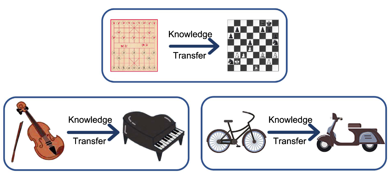](https://mlsysbook.ai/contents/core/ondevice_learning/images/png/ondevice_transfer_learning_apps.png "Figure 1: Knowledge Transfer: Pretrained models accelerate learning on new tasks by leveraging existing representations, as seen by adapting skills between related board games or musical instruments. This transfer extends across domains like bicycle riding and scooter operation, where shared underlying structures allow efficient adaptation with limited new data.")
Figure 1: Knowledge Transfer: Pretrained models accelerate learning on new tasks by leveraging existing representations, as seen by adapting skills between related board games or musical instruments. This transfer extends across domains like bicycle riding and scooter operation, where shared underlying structures allow efficient adaptation with limited new data.
This conceptual shift, enabled by transfer learning and adaptation, enables real-world on-device applications. Whether adapting a language model for personal typing preferences, adjusting gesture recognition to individual movement patterns, or recalibrating a sensor model in changing environments, on-device learning allows systems to remain responsive, efficient, and user-aligned over time.
### Real-World Application Domains
Building on these established motivations (personalization, latency, privacy, and infrastructure efficiency), real-world deployments demonstrate the practical impact of on-device learning across diverse application domains. These domains span consumer technologies, healthcare, industrial systems, and embedded applications, each showcasing scenarios where the benefits outlined above become essential for effective machine learning deployment.
Mobile input prediction represents the most mature and widely deployed example of on-device learning. In systems such as smartphone keyboards, predictive text and autocorrect features benefit substantially from continuous local adaptation. User typing patterns are highly personalized and evolve dynamically, making centralized static models insufficient for optimal user experience. On-device learning allows language models to fine-tune their predictions directly on the device, achieving personalization while maintaining data locality.
For instance, Google’s Gboard employs federated learning to improve shared models across a large population of users while keeping raw data local to each device ([Hard et al. 2018](https://mlsysbook.ai/contents/core/ondevice_learning/ondevice_learning.html#ref-hard2018federated)
)[4](https://mlsysbook.ai/contents/core/ondevice_learning/ondevice_learning.html#fn4)
.
Hard, Andrew, Kanishka Rao, Rajiv Mathews, Saurabh Ramaswamy, Françoise Beaufays, Sean Augenstein, Hubert Eichner, Chloé Kiddon, and Daniel Ramage. 2018. “Federated Learning for Mobile Keyboard Prediction.” In _International Conference on Learning Representations (ICLR)_.
4 **Gboard Federated Pioneer**: Gboard became the first major commercial federated learning deployment in 2017, processing updates from over 1 billion devices. The technical challenge was immense: aggregating model updates while ensuring no individual user’s typing patterns could be inferred. Google’s success with Gboard proved federated learning could work at planetary scale, demonstrating 10-20% accuracy improvements over static models while maintaining strict differential privacy guarantees.
As shown in [Figure 2](https://mlsysbook.ai/contents/core/ondevice_learning/ondevice_learning.html#fig-ondevice-gboard)
, different prediction strategies illustrate how local adaptation operates in real time: next-word prediction (NWP) suggests likely continuations based on prior text, while Smart Compose uses on-the-fly rescoring to offer dynamic completions, demonstrating the sophistication of local inference mechanisms.
[](https://mlsysbook.ai/contents/core/ondevice_learning/images/png/ondevice_gboard_example.png "Figure 2: On-Device Prediction Strategies: Gboard employs both next-word prediction and smart compose with on-the-fly rescoring to adapt to user typing patterns locally, enhancing personalization and preserving privacy. These techniques demonstrate how machine learning models can refine predictions in real time without transmitting data to a central server, enabling efficient and private mobile input experiences.")
Figure 2: On-Device Prediction Strategies: Gboard employs both next-word prediction and smart compose with on-the-fly rescoring to adapt to user typing patterns locally, enhancing personalization and preserving privacy. These techniques demonstrate how machine learning models can refine predictions in real time without transmitting data to a central server, enabling efficient and private mobile input experiences.
Building on the consumer applications, wearable and health monitoring devices present equally compelling use cases with additional regulatory constraints. These systems rely on real-time data from accelerometers, heart rate sensors, and electrodermal activity monitors to track user health and fitness. Physiological baselines vary dramatically between individuals, creating a personalization challenge that static models cannot address effectively. On-device learning allows models to adapt to these individual baselines over time, substantially improving the accuracy of activity recognition, stress detection, and sleep staging while meeting regulatory requirements for data localization.
Voice interaction technologies present another important application domain with unique acoustic challenges. Wake-word detection[5](https://mlsysbook.ai/contents/core/ondevice_learning/ondevice_learning.html#fn5)
and voice interfaces in devices such as smart speakers and earbuds must recognize voice commands quickly and accurately, even in noisy or dynamic acoustic environments.
5 **Wake-Word Detection**: Always-listening keyword spotting that activates voice assistants (“Hey Siri,” “OK Google,” “Alexa”). These systems run continuously at ~1 mW power consumption, roughly 1000\\(\\times\\) less than full speech recognition. They use tiny neural networks (~100 KB) with specialized architectures optimized for sub-100 ms latency and minimal false positive rates (<0.1 activations per hour). Modern systems achieve 95%+ accuracy while processing 16 kHz audio in real-time, making on-device personalization critical for adapting to individual voice characteristics and reducing false activations.
These systems face strict latency requirements: voice interfaces must maintain end-to-end response times under 500 ms to preserve natural conversation flow, with wake-word detection requiring sub-100 ms response times to avoid user frustration. Local training allows models to adapt to the user’s unique voice profile and changing ambient context, reducing false positives and missed detections while meeting these demanding performance constraints. This adaptation proves particularly valuable in far-field audio settings, where microphone configurations and room acoustics vary dramatically across deployments.
Beyond consumer applications, industrial IoT and remote monitoring systems demonstrate the value of on-device learning in resource-constrained environments. In applications such as agricultural sensing, pipeline monitoring, or environmental surveillance, connectivity to centralized infrastructure may be limited, expensive, or entirely unavailable. On-device learning allows these systems to detect anomalies, adjust thresholds, or adapt to seasonal trends without continuous communication with the cloud. This capability proves necessary for maintaining autonomy and reliability in edge-deployed sensor networks, where system downtime or missed detections can have significant economic or safety consequences.
The most demanding applications emerge in embedded computer vision systems, including those in robotics, AR/VR, and smart cameras, which combine complex visual processing with extreme timing constraints. Camera applications must process frames within 33 ms to maintain 30 FPS real-time performance, while AR/VR systems demand motion-to-photon latencies under 20 ms to prevent nausea and maintain immersion. Safety-critical control systems require even tighter bounds, typically under 10 ms, where delayed decisions can have severe consequences. These systems operate in novel or rapidly changing environments that differ substantially from their original training conditions. On-device adaptation allows models to recalibrate to new lighting conditions, object appearances, or motion patterns while meeting these critical latency budgets that fundamentally drive the architectural decision between on-device versus cloud-based processing.
Each domain reveals a common pattern: deployment environments introduce variation and context-specific requirements that cannot be anticipated during centralized training. These applications demonstrate how the motivational drivers (personalization, latency, privacy, and infrastructure efficiency) manifest as concrete engineering constraints. Mobile keyboards face memory limitations for storing user-specific patterns, wearable devices encounter energy budgets that restrict training frequency, voice interfaces must meet sub-100 ms latency requirements that preclude cloud coordination, and industrial IoT systems operate in network-constrained environments that demand autonomous adaptation. This pattern illuminates the fundamental design requirement shaping all subsequent technical decisions: learning must be performed efficiently, privately, and reliably under significant resource constraints that we examine through constraint analysis ([Section 1.3](https://mlsysbook.ai/contents/core/ondevice_learning/ondevice_learning.html#sec-ondevice-learning-design-constraints-c776)
), adaptation techniques ([Section 1.4](https://mlsysbook.ai/contents/core/ondevice_learning/ondevice_learning.html#sec-ondevice-learning-model-adaptation-6a82)
), and federated coordination ([Section 1.6](https://mlsysbook.ai/contents/core/ondevice_learning/ondevice_learning.html#sec-ondevice-learning-federated-learning-6e7e)
).
### Architectural Trade-offs: Centralized vs. Decentralized Training
These applications demonstrate the practical value of on-device learning across diverse domains. Building on this foundation, we now examine how on-device learning differs from traditional ML architectures, revealing a complete reimagining of the training lifecycle that extends far beyond simple deployment choices.
Understanding the shift that on-device learning represents requires examining how traditional machine learning systems are structured and where their limitations become apparent. Most machine learning systems today follow a centralized learning paradigm that has served the field well but increasingly shows strain under modern deployment requirements. Models are trained in data centers using large-scale, curated datasets aggregated from many sources. Once trained, these models are deployed to client devices in a static form, where they perform inference without further modification. Updates to model parameters, either to incorporate new data or to improve generalization, are handled periodically through offline retraining, often using newly collected or labeled data sent back from the field.
This established centralized model offers numerous proven advantages: high-performance computing infrastructure, access to diverse data distributions, and robust debugging and validation pipelines. It also depends on several assumptions that may not hold in modern deployment scenarios: reliable data transfer, trust in data custodianship, and infrastructure capable of managing global updates across device fleets. As machine learning is deployed into increasingly diverse and distributed environments, the limitations of this approach become more apparent and often prohibitive.
In contrast to this centralized approach, on-device learning embraces an inherently decentralized paradigm that challenges many traditional assumptions. Each device maintains its own copy of a model and adapts it locally using data that is typically unavailable to centralized infrastructure. Training occurs on-device, often asynchronously and under varying resource conditions that change based on device usage patterns, battery levels, and thermal states. Data never leaves the device, reducing privacy exposure but also complicating coordination between devices. Devices may differ dramatically in their hardware capabilities, runtime environments, and patterns of use, making the learning process heterogeneous and difficult to standardize. These hardware variations create significant system design challenges.
This decentralized architecture introduces a new class of systems challenges that extend well beyond traditional machine learning concerns. Devices may operate with different versions of the model, leading to inconsistencies in behavior across the deployment fleet. Evaluation and validation become significantly more complex, as there is no central point from which to measure performance across all devices ([McMahan et al. 2017](https://mlsysbook.ai/contents/core/ondevice_learning/ondevice_learning.html#ref-mcmahan2017communication)
). Model updates must be carefully managed to prevent degradation, and safety guarantees become substantially harder to enforce in the absence of centralized testing and validation infrastructure.
Bonawitz, Keith, Hubert Eichner, Wolfgang Grieskamp, Dzmitry Huba, Alex Ingerman, Vladimir Ivanov, Chloe Kiddon, et al. 2019. “Towards Federated Learning at Scale: System Design,” February. [http://arxiv.org/abs/1902.01046v2](http://arxiv.org/abs/1902.01046v2)
.
Managing thousands of heterogeneous edge devices exceeds typical distributed systems complexity. Device heterogeneity extends beyond hardware differences to include varying operating system versions, security patches, network configurations, and power management policies. At any given time, 20-40% of devices are offline ([Bonawitz et al. 2019](https://mlsysbook.ai/contents/core/ondevice_learning/ondevice_learning.html#ref-bonawitz2019towards)
), while others have been disconnected for weeks or months, creating persistent coordination challenges.
When disconnected devices reconnect, they require state reconciliation to avoid version conflicts. Update verification becomes critical as devices can silently fail to apply updates or report success while running outdated models. Robust systems implement multi-stage verification: cryptographic signatures confirm update integrity, functional tests validate model behavior, and telemetry confirms deployment success. Rollback strategies must handle partial deployments where some devices received updates while others remain on previous versions, requiring sophisticated orchestration to maintain system consistency during failure recovery.
These challenges require different approaches to system design and operational management compared to centralized ML systems, building on the distributed systems principles from **[Chapter 13: ML Operations](https://mlsysbook.ai/contents/core/ops/ops.html#sec-ml-operations)
** while introducing edge-specific complexities.
Despite these challenges, decentralization introduces opportunities that often justify the additional complexity. It allows for deep personalization without centralized oversight, supports robust learning in disconnected or bandwidth-limited environments, and reduces the operational cost and infrastructure burden for model updates. Realizing these benefits raises questions of how to effectively coordinate learning across devices, whether through periodic synchronization, federated aggregation, or hybrid approaches that balance local and global objectives.
The move from centralized to decentralized learning represents more than a shift in deployment architecture. It reshapes the entire design space for machine learning systems, requiring new approaches to model architecture, training algorithms, data management, and system validation. In centralized training, data is aggregated from many sources and processed in large-scale data centers, where models are trained, validated, and then deployed in a static form to edge devices. In contrast, on-device learning introduces a fundamentally different paradigm: models are updated directly on client devices using local data, often asynchronously and under diverse hardware conditions. This architectural transformation introduces coordination challenges while enabling autonomous local adaptation, requiring careful consideration of validation, system reliability, and update orchestration across heterogeneous device populations.
On-device learning responds to the limitations of centralized machine learning workflows. The transformation from centralized to decentralized learning creates three distinct operational phases, each with different characteristics and challenges.
The traditional centralized paradigm begins with cloud-based training on aggregated data, followed by static model deployment to client devices. This approach works well when data collection is feasible, network connectivity is reliable, and a single global model can serve all users effectively. However, it breaks down when data becomes personalized, privacy-sensitive, or collected in environments with limited connectivity.
Once deployed, local differences begin to emerge as each device encounters its own unique data distribution. Devices collect data that reflects individual user patterns, environmental conditions, and usage contexts. This data is often non-IID (non-independent and identically distributed)[6](https://mlsysbook.ai/contents/core/ondevice_learning/ondevice_learning.html#fn6)
and noisy, requiring local model adaptation to maintain performance. This transition marks the shift from global generalization to local specialization.
6 **Non-IID (Non-Independent and Identically Distributed)**: In machine learning, data is IID when samples are drawn independently from the same distribution. Non-IID violates this assumption, common in federated learning where each device collects data from different users, environments, or use cases. For example, smartphone keyboard data varies dramatically between users (languages, writing styles, autocorrect needs), making personalized model training essential but challenging for convergence.
The final phase introduces federated coordination, where devices periodically synchronize their local adaptations through aggregated model updates rather than raw data sharing. This enables privacy-preserving global refinement while maintaining the benefits of local personalization.
These three distinct phases (centralized training, local adaptation, and federated coordination) represent an architectural evolution that reshapes every aspect of the machine learning lifecycle. [Figure 3](https://mlsysbook.ai/contents/core/ondevice_learning/ondevice_learning.html#fig-centralized-vs-decentralized)
illustrates how data flow, computational distribution, and coordination mechanisms differ across these phases, highlighting the increasing complexity but also the enhanced capabilities that emerge at each stage. Understanding this progression helps frame the challenges that on-device learning systems must address.
[](https://mlsysbook.ai/contents/core/ondevice_learning/cee3e9981ee09d7c65e151839ec0b5d45964502d.svg "Figure 3: The evolution from centralized cloud training (region A) through local device adaptation (region B) to federated coordination (region C) represents a fundamental shift in machine learning architecture. Each phase introduces distinct operational characteristics, from uniform global models to personalized local adaptations to coordinated distributed learning.")
Figure 3: The evolution from centralized cloud training (region A) through local device adaptation (region B) to federated coordination (region C) represents a fundamental shift in machine learning architecture. Each phase introduces distinct operational characteristics, from uniform global models to personalized local adaptations to coordinated distributed learning.
**Self-Check: Question 1.2**
1. Which of the following is a primary benefit of on-device learning compared to centralized learning?
1. Increased computational power
2. Simplified model management
3. Enhanced personalization and privacy
4. Lower development costs
2. Describe a scenario where on-device learning is more advantageous than centralized learning, considering privacy and latency.
3. True or False: On-device learning eliminates the need for centralized model updates.
4. On-device learning allows for model adaptation using \_\_\_\_ data, enhancing personalization and privacy.
[See Answers →](https://mlsysbook.ai/contents/core/ondevice_learning/ondevice_learning.html#quiz-answer-sec-ondevice-learning-motivations-benefits-37c3)
Design Constraints
------------------
Part III established efficiency principles that shape all machine learning systems. **[Chapter 9: Efficient AI](https://mlsysbook.ai/contents/core/efficient_ai/efficient_ai.html#sec-efficient-ai)
** introduced three efficiency dimensions (algorithmic, compute, and data efficiency) and revealed through scaling laws why brute-force approaches hit fundamental limits. **[Chapter 10: Model Optimizations](https://mlsysbook.ai/contents/core/optimizations/optimizations.html#sec-model-optimizations)
** developed compression techniques including quantization, pruning, and knowledge distillation that enable deployment on resource-constrained devices. **[Chapter 11: AI Acceleration](https://mlsysbook.ai/contents/core/hw_acceleration/hw_acceleration.html#sec-ai-acceleration)
** characterized edge hardware capabilities from microcontrollers to mobile accelerators, as detailed in the hardware discussions. These chapters focused primarily on inference workloads: running pre-trained models efficiently.
On-device learning operates under these same efficiency constraints but with training-specific amplifications that make optimization dramatically more challenging. Where inference requires a single forward pass through the network, training demands forward propagation, gradient computation through backpropagation, and weight updates, increasing memory requirements by 3-5\\(\\times\\) and computational costs by 2-3\\(\\times\\). The model compression techniques that enable efficient inference become baseline requirements rather than optimizations, as training within edge device constraints would be impossible without aggressive compression.
Given the established motivations for on-device learning, we now examine the fundamental engineering challenges that shape its implementation. Enabling learning on the device requires completely rethinking conventional assumptions about where and how machine learning systems operate. In centralized environments, models are trained with access to extensive compute infrastructure, large and curated datasets, and generous memory and energy budgets. At the edge, none of these assumptions hold, creating a fundamentally different design space.
On-device learning constraints fall into three critical dimensions that parallel but extend the efficiency framework from Part III: model compression requirements (extending algorithmic efficiency), sparse and non-uniform data characteristics (extending data efficiency), and severely limited computational resources (extending compute efficiency). These three dimensions form an interconnected constraint space that defines the feasible region for on-device learning systems, with each dimension imposing distinct limitations that influence algorithmic choices, system architecture, and deployment strategies.
### Quantifying Training Overhead on Edge Devices
The transition from inference-only deployment to on-device training creates multiplicative rather than additive complexity. These constraints interact and amplify each other in ways that reshape system design requirements, building on the resource optimization principles from **[Chapter 9: Efficient AI](https://mlsysbook.ai/contents/core/efficient_ai/efficient_ai.html#sec-efficient-ai)
** while introducing new challenges specific to distributed learning environments.
The efficiency constraints introduced in Part III apply to both inference and training, but training amplifies each constraint dimension by 3-10\\(\\times\\). [Table 1](https://mlsysbook.ai/contents/core/ondevice_learning/ondevice_learning.html#tbl-training-amplification)
quantifies how training workloads intensify the challenges established in **[Chapter 9: Efficient AI](https://mlsysbook.ai/contents/core/efficient_ai/efficient_ai.html#sec-efficient-ai)
**, **[Chapter 10: Model Optimizations](https://mlsysbook.ai/contents/core/optimizations/optimizations.html#sec-model-optimizations)
**, and **[Chapter 11: AI Acceleration](https://mlsysbook.ai/contents/core/hw_acceleration/hw_acceleration.html#sec-ai-acceleration)
**.
These amplifications explain why simply applying Part III optimization techniques to training workloads proves insufficient. Each constraint category shapes on-device learning system design, requiring approaches that build on but extend beyond the inference-focused methods from earlier chapters.
Table 1: **Training Amplifies Inference Constraints**: On-device learning operates under the same efficiency constraints as inference (Part III) but with training-specific amplifications that make optimization dramatically more challenging. This table quantifies how each constraint dimension intensifies when transitioning from running pre-trained models to adapting them locally. Amplification factors assume standard backpropagation without optimizations like gradient checkpointing.
| | | | |
| --- | --- | --- | --- |
| **Memory Footprint** | Model weights + single activation map | Weights + full activation cache + gradients + optimizer state | 3-5\\(\\times\\) increase; forces aggressive compression |
| **Compute Operations** | Forward pass only | Forward + backward + weight update | 2-3\\(\\times\\) increase; limits model complexity |
| **Memory Bandwidth** | Sequential weight reads | Bidirectional data flow for gradients | 5-10\\(\\times\\) increase; creates bottlenecks |
| **Energy per Sample** | Single inference operation | Multiple gradient steps with convergence | 10-50\\(\\times\\) increase; requires opportunistic scheduling |
| **Data Requirements** | Pre-collected, curated datasets | Sparse, noisy, streaming local data | Necessitates sample-efficient methods |
| **Hardware Utilization** | Optimized for forward passes | Different access patterns for backprop | Inference accelerators may not help training |
[Figure 4](https://mlsysbook.ai/contents/core/ondevice_learning/ondevice_learning.html#fig-ondevice-pretraining)
illustrates a pipeline that combines offline pre-training with online adaptive learning on resource-constrained IoT devices. The system first undergoes meta-training with generic data. During deployment, device-specific constraints such as data availability, compute, and memory shape the adaptation strategy by ranking and selecting layers and channels to update. This allows efficient on-device learning within limited resource envelopes.
[](https://mlsysbook.ai/contents/core/ondevice_learning/c42ceee9cd4bc594efd92af96f7dfce696ac282b.svg "Figure 4: Resource-constrained devices use a two-stage learning process: offline pre-training establishes initial model weights, followed by online adaptation that selectively updates layers based on available data, compute, and memory. This approach balances model performance with the practical limitations of edge deployment, enabling continuous learning in real-world environments.")
Figure 4: Resource-constrained devices use a two-stage learning process: offline pre-training establishes initial model weights, followed by online adaptation that selectively updates layers based on available data, compute, and memory. This approach balances model performance with the practical limitations of edge deployment, enabling continuous learning in real-world environments.
### Model Constraints
The first dimension of on-device learning constraints centers on the model itself. Its structure, size, and computational requirements determine deployment feasibility. The structure and size of the machine learning model directly influence whether on-device training is even possible, let alone practical. Unlike cloud-deployed models that can span billions of parameters and rely on multi-gigabyte memory budgets, models intended for on-device learning must conform to tight constraints on memory, storage, and computational complexity. These constraints apply not only at inference time, but become even more restrictive during training, where additional resources are needed for gradient computation, parameter updates, and optimizer state management.
The scale of these constraints becomes apparent when examining specific examples across the device spectrum. The MobileNetV2 architecture, commonly used in mobile vision tasks, requires approximately 14 MB of storage in its standard configuration. While this memory requirement is entirely feasible for modern smartphones with gigabytes of available RAM, it far exceeds the memory available on embedded microcontrollers such as the Arduino Nano 33 BLE Sense[7](https://mlsysbook.ai/contents/core/ondevice_learning/ondevice_learning.html#fn7)
, which provides only 256 KB of SRAM and 1 MB of flash storage. This dramatic difference in available resources necessitates aggressive model compression techniques. In such severely constrained platforms, even a single layer of a typical convolutional neural network may exceed available RAM during training due to the need to store intermediate feature maps and gradient information.
7 **Arduino Edge Computing Reality**: The Arduino Nano 33 BLE Sense represents typical microcontroller constraints: 256 KB SRAM is roughly 65,000 times smaller than a modern smartphone’s 16 GB RAM (flagship devices). To put this in perspective, storing just one 224×224×3 RGB image (150 KB) would consume 60% of available memory. Training requires 3-5\\(\\times\\) more memory for gradients and activations, making even tiny models challenging. The 1 MB flash storage can hold only the smallest quantized models, forcing designers to use 8-bit or even 4-bit representations.
Beyond static storage requirements, the training process itself dramatically expands the effective memory footprint, creating an additional layer of constraint. Standard backpropagation requires caching activations for each layer during the forward pass, which are then reused during gradient computation in the backward pass. As established in the amplification analysis above, this activation caching multiplies memory requirements compared to inference-only deployment. For a seemingly modest 10-layer convolutional model processing \\(64 \\times 64\\) images, the required memory may exceed 1 to 2 MB, well beyond the SRAM capacity of most embedded systems and highlighting the fundamental tension between model expressiveness and resource availability.
Compounding these memory constraints, model complexity directly affects runtime energy consumption and thermal limits, introducing additional practical barriers to deployment. In systems such as smartwatches or battery-powered wearables, sustained model training can rapidly deplete energy reserves or trigger thermal throttling that degrades performance. Training a full model using floating-point operations on these devices is often infeasible from an energy perspective, even when memory constraints are satisfied. These practical limitations have motivated the development of ultra-lightweight model variants, such as MLPerf Tiny benchmark networks ([Banbury et al. 2021](https://mlsysbook.ai/contents/core/ondevice_learning/ondevice_learning.html#ref-banbury2021mlperf)
), which fit within 100–200 KB and can be adapted using only partial gradient updates. These specialized models employ aggressive quantization and pruning strategies to achieve such compact representations while maintaining sufficient expressiveness for meaningful adaptation.
Banbury, Colby, Vijay Janapa Reddi, Peter Torelli, Jeremy Holleman, Nat Jeffries, Csaba Kiraly, Pietro Montino, et al. 2021. “MLPerf Tiny Benchmark.” _arXiv Preprint arXiv:2106.07597_, June. [http://arxiv.org/abs/2106.07597v4](http://arxiv.org/abs/2106.07597v4)
.
The practical implications of battery and thermal constraints extend beyond just limiting training duration. Mobile devices must carefully balance training opportunities with user experience. Aggressive on-device training can cause noticeable device heating and rapid battery drain, leading to user dissatisfaction and potential app uninstalls. Modern smartphones typically limit sustained processing to 2-3 W for ML workloads to prevent thermal discomfort, though they can burst to 5-10 W for brief periods before thermal throttling kicks in. Training even modest models can easily exceed these sustainable power limits. This reality necessitates intelligent scheduling strategies: training during charging periods when thermal dissipation is improved, utilizing low-power cores for gradient computation when possible, and implementing thermal-aware duty cycling that pauses training when temperature thresholds are exceeded. Some systems even leverage device usage patterns, scheduling intensive adaptation only during overnight charging when the device is idle and connected to power.
Given these multifaceted constraints, the model architecture itself must be fundamentally designed with on-device learning capabilities in mind from the outset. Many conventional architectures, such as large transformers or deep convolutional networks, are simply not viable for on-device adaptation due to their inherent size and computational complexity. Instead, specialized lightweight architectures such as MobileNets[8](https://mlsysbook.ai/contents/core/ondevice_learning/ondevice_learning.html#fn8)
, SqueezeNet ([Iandola et al. 2016](https://mlsysbook.ai/contents/core/ondevice_learning/ondevice_learning.html#ref-iandola2016squeezenet)
), and EfficientNet ([Tan and Le 2019](https://mlsysbook.ai/contents/core/ondevice_learning/ondevice_learning.html#ref-tan2019efficientnet)
) have been developed specifically for resource-constrained environments. These architectures leverage efficiency principles and architectural optimizations, rethinking how neural networks can be structured. These specialized models employ techniques such as depthwise separable convolutions[9](https://mlsysbook.ai/contents/core/ondevice_learning/ondevice_learning.html#fn9)
, bottleneck layers, and aggressive quantization to dramatically reduce memory and compute requirements while maintaining sufficient performance for practical applications.
8 **MobileNet Innovation**: Google’s MobileNet family revolutionized mobile AI by achieving 10-20\\(\\times\\) parameter reduction compared to traditional CNNs. MobileNetV1 (2017) used depthwise separable convolutions to reduce floating-point operations (FLOPs) by 8-9\\(\\times\\), while MobileNetV2 (2018) added inverted residuals and linear bottlenecks. The breakthrough allowed real-time inference on smartphones: MobileNetV2 runs ImageNet classification in ~75 ms on a Pixel phone versus 1.8 seconds for ResNet-50 ([He et al. 2016](https://mlsysbook.ai/contents/core/ondevice_learning/ondevice_learning.html#ref-he2016deep)
).
He, Kaiming, Xiangyu Zhang, Shaoqing Ren, and Jian Sun. 2016. “Deep Residual Learning for Image Recognition.” In _2016 IEEE Conference on Computer Vision and Pattern Recognition (CVPR)_, 770–78. IEEE. [https://doi.org/10.1109/cvpr.2016.90](https://doi.org/10.1109/cvpr.2016.90)
.
Iandola, Forrest N., Song Han, Matthew W. Moskewicz, Khalid Ashraf, William J. Dally, and Kurt Keutzer. 2016. “SqueezeNet: AlexNet-Level Accuracy with 50x Fewer Parameters and <0.5MB Model Size,” February. [http://arxiv.org/abs/1602.07360v4](http://arxiv.org/abs/1602.07360v4)
.
Tan, Mingxing, and Quoc V. Le. 2019. “EfficientNet: Rethinking Model Scaling for Convolutional Neural Networks.” In _Proceedings of the International Conference on Machine Learning (ICML)_, 6105–14.
9 **Depthwise Separable Convolutions**: This technique decomposes standard convolution into two operations: depthwise convolution (applies single filter per input channel) and pointwise convolution (1×1 conv to combine channels). For a 3×3 conv with 512 input/output channels, standard convolution requires 2.4 M parameters while depthwise separable needs only 13.8 K, a 174\\(\\times\\) reduction. The computational savings are similarly dramatic, making real-time inference possible on mobile CPUs.
Howard, Andrew G., Menglong Zhu, Bo Chen, Dmitry Kalenichenko, Weijun Wang, Tobias Weyand, Marco Andreetto, and Hartwig Adam. 2017. “MobileNets: Efficient Convolutional Neural Networks for Mobile Vision Applications.” _CoRR_ abs/1704.04861 (April). [http://arxiv.org/abs/1704.04861v1](http://arxiv.org/abs/1704.04861v1)
.
These architectures are often designed to be modular, allowing for easy adaptation and fine-tuning. For example, MobileNets ([Howard et al. 2017](https://mlsysbook.ai/contents/core/ondevice_learning/ondevice_learning.html#ref-howard2017mobilenets)
) can be configured with different width multipliers and resolution settings to balance performance and resource usage. Concretely, MobileNetV2 with α=1.0 requires 3.4 M parameters (13.6 MB in FP32), but with α=0.5 this drops to 0.7 M parameters (2.8 MB), enabling deployment on devices with just 4 MB available RAM. This flexibility is important for on-device learning, where the model must adapt to the specific constraints of the deployment environment.
While model architecture determines the memory and computational baseline for on-device learning, the characteristics of available training data introduce equally fundamental limitations that shape every aspect of the learning process.
### Data Constraints
The second dimension of on-device learning constraints centers on data availability and quality. The nature of data available to on-device ML systems differs dramatically from the large, curated, and centrally managed datasets used in cloud-based training. At the edge, data is locally collected, temporally sparse, and often unstructured or unlabeled, creating a different learning environment. These characteristics introduce multifaceted challenges in volume, quality, and statistical distribution, all of which directly affect the reliability and generalizability of learning on the device.
Data volume represents the first major constraint, severely limited by both storage constraints and the sporadic nature of user interaction. For example, a smart fitness tracker may collect motion data only during physical activity, generating relatively few labeled samples per day. If a user wears the device for just 30 minutes of exercise, only a few hundred data points might be available for training, compared to the thousands or millions typically required for effective supervised learning in controlled environments. This scarcity changes the learning paradigm from data-rich to data-efficient algorithms.
Beyond volume limitations, on-device data is frequently non-IID (non-independent and identically distributed) ([Zhao et al. 2018](https://mlsysbook.ai/contents/core/ondevice_learning/ondevice_learning.html#ref-zhao2018federated)
), creating statistical challenges that cloud-based systems rarely encounter. This heterogeneity manifests across multiple dimensions: user behavior patterns, environmental conditions, linguistic preferences, and usage contexts. A voice assistant deployed across households encounters dramatic variation in accents, languages, speaking styles, and command patterns. Similarly, smartphone keyboards adapt to individual typing patterns, autocorrect preferences, and multilingual usage that varies dramatically between users. This data heterogeneity complicates both model convergence and the design of update mechanisms that must generalize across devices while maintaining personalization.
Zhao, Yue, Meng Li, Liangzhen Lai, Naveen Suda, Damon Civin, and Vikas Chandra. 2018. “Federated Learning with Non-IID Data.” _CoRR_ abs/1806.00582 (June). [http://arxiv.org/abs/1806.00582v2](http://arxiv.org/abs/1806.00582v2)
.
Compounding these distribution challenges, label scarcity presents an additional critical obstacle that severely limits traditional learning approaches. Most edge-collected data is unlabeled by default, requiring systems to learn from weak or implicit supervision signals. In a smartphone camera, for instance, the device may capture thousands of images throughout the day, but only a few are associated with meaningful user actions (e.g., tagging, favoriting, or sharing), which could serve as implicit labels. In many applications, including detecting anomalies in sensor data and adapting gesture recognition models, explicit labels may be entirely unavailable, making traditional supervised learning infeasible without developing alternative methods for weak supervision or unsupervised adaptation.
Data quality issues add another layer of complexity to the on-device learning challenge. Noise and variability further degrade the already limited data available for training. Embedded systems such as environmental sensors or automotive ECUs may experience fluctuations in sensor calibration, environmental interference, or mechanical wear, leading to corrupted or drifting input signals over time. Without centralized validation systems to detect and filter these errors, they may silently degrade learning performance, creating a reliability challenge that cloud-based systems can more easily address through data preprocessing pipelines.
Finally, data privacy and security concerns impose the most restrictive constraints of all, often making data sharing architecturally impossible rather than merely undesirable. Sensitive information, such as health data, personal communications, or user behavioral patterns, must be protected from unauthorized access under legal and ethical requirements. This constraint often completely precludes the use of traditional data-sharing methods, such as uploading raw data to a central server for training. Instead, on-device learning must rely on sophisticated techniques that enable local adaptation without ever exposing sensitive information, changing how learning systems can be designed and validated.
### Compute Constraints
**[Chapter 11: AI Acceleration](https://mlsysbook.ai/contents/core/hw_acceleration/hw_acceleration.html#sec-ai-acceleration)
** characterized the edge hardware landscape that provides computational substrate for machine learning: microcontrollers like STM32F4 and ESP32 at the most constrained end, mobile-class processors with dedicated AI accelerators (Apple Neural Engine, Qualcomm Hexagon, Google Tensor) in the middle, and high-capability edge devices at the upper end. That chapter focused on inference capabilities—the computational throughput, memory bandwidth, and energy efficiency achievable when executing pre-trained models.
Training workloads exhibit fundamentally different computational characteristics that reshape hardware utilization patterns. Building on the edge hardware landscape characterized in **[Chapter 11: AI Acceleration](https://mlsysbook.ai/contents/core/hw_acceleration/hw_acceleration.html#sec-ai-acceleration)
**, from microcontrollers to mobile AI accelerators, on-device learning must operate within severely constrained computational envelopes that differ dramatically from cloud-based training infrastructure by factors of hundreds or thousands in raw computational capacity.
The key difference: backpropagation requires significantly higher memory bandwidth than inference due to gradient computation and activation caching, weight updates create write-heavy access patterns unlike inference’s read-only operations, and optimizer state management demands additional memory allocation that inference never encounters. These training-specific demands mean hardware perfectly adequate for inference may prove entirely inadequate for adaptation, even when updating only a small parameter subset.
At the most constrained end of the spectrum, devices such as the STM32F4[10](https://mlsysbook.ai/contents/core/ondevice_learning/ondevice_learning.html#fn10)
or ESP32[11](https://mlsysbook.ai/contents/core/ondevice_learning/ondevice_learning.html#fn11)
microcontrollers offer only a few hundred kilobytes of SRAM and completely lack hardware support for floating-point operations ([Warden and Situnayake 2020](https://mlsysbook.ai/contents/core/ondevice_learning/ondevice_learning.html#ref-lai2020tinyml)
). These extreme constraints represent the fundamental limitations of edge hardware (**[Chapter 11: AI Acceleration](https://mlsysbook.ai/contents/core/hw_acceleration/hw_acceleration.html#sec-ai-acceleration)
**). Such severe limitations preclude the use of conventional deep learning libraries and require models to be meticulously designed for integer arithmetic and minimal runtime memory allocation. In these environments, even apparently simple models require highly specialized techniques, including quantization-aware training[12](https://mlsysbook.ai/contents/core/ondevice_learning/ondevice_learning.html#fn12)
and selective parameter updates, to execute training loops without exceeding memory or power budgets.
10 **STM32F4 Microcontroller Reality**: The STM32F4 represents the harsh reality of embedded computing: 192 KB SRAM (roughly the size of a small JPEG image) and 1 MB flash storage, running at 168 MHz without floating-point hardware acceleration. Integer arithmetic is 10-100\\(\\times\\) slower than dedicated floating-point units found in mobile chips. Power consumption is ~100 mW during active processing, requiring careful duty-cycling to preserve battery life. These constraints make even simple neural networks challenging: a 10-neuron hidden layer requires ~40 KB for weights alone in FP32.
11 **ESP32 Edge Computing**: The ESP32 provides 520 KB SRAM and dual-core processing at 240 MHz, making it more capable than STM32F4 but still severely constrained. Its key advantage is built-in WiFi and Bluetooth for federated learning scenarios. However, the lack of hardware floating-point support means all ML operations must use integer quantization. Real-world deployments show 8-bit quantized models can achieve 95% of FP32 accuracy while fitting in ~50 KB memory, enabling basic on-device training for simple tasks like sensor anomaly detection.
Warden, Pete, and Daniel Situnayake. 2020. _TinyML: Machine Learning with TensorFlow Lite on Arduino and Ultra-Low-Power Microcontrollers_. O’Reilly Media.
12 **Quantization-Aware Training**: Unlike post-training quantization which converts trained FP32 models to INT8, quantization-aware training simulates low-precision arithmetic during training itself. This allows the model to learn robust representations despite reduced precision. Critical for edge devices where INT8 operations consume \\(4\\times\\) less power and enable \\(4\\times\\) faster inference compared to FP32, while maintaining 95-99% of original accuracy.
13 **Stochastic Gradient Descent (SGD)**: The fundamental optimization algorithm for neural networks, updating parameters using gradients computed on small batches (or single samples). Unlike full-batch gradient descent, SGD’s randomness helps escape local minima while requiring minimal memory, storing only current parameters and gradients. This simplicity makes SGD ideal for microcontrollers where advanced optimizers like Adam would exceed memory budgets.
The practical implications are stark: while the STM32F4 microcontroller can run a simple linear regression model with a few hundred parameters, training even a small convolutional neural network would immediately exceed its memory capacity. In these severely constrained environments, training is often limited to simple algorithms such as stochastic gradient descent (SGD)[13](https://mlsysbook.ai/contents/core/ondevice_learning/ondevice_learning.html#fn13)
or \\(k\\)\-means clustering, which can be implemented using integer arithmetic and minimal memory overhead, representing a fundamental departure from modern machine learning practice.
Moving up the computational hierarchy, mobile-class hardware represents a significant improvement but still operates under substantial constraints. Platforms including the Qualcomm Snapdragon, Apple Neural Engine[14](https://mlsysbook.ai/contents/core/ondevice_learning/ondevice_learning.html#fn14)
, and Google Tensor SoC[15](https://mlsysbook.ai/contents/core/ondevice_learning/ondevice_learning.html#fn15)
provide significantly more compute power than microcontrollers, often featuring dedicated AI accelerators and optimized support for 8-bit or mixed-precision[16](https://mlsysbook.ai/contents/core/ondevice_learning/ondevice_learning.html#fn16)
matrix operations. These accelerators, their capabilities, and their programming models are detailed in **[Chapter 11: AI Acceleration](https://mlsysbook.ai/contents/core/hw_acceleration/hw_acceleration.html#sec-ai-acceleration)
**. While these platforms can support more sophisticated training routines, including full backpropagation over compact models, they still fall dramatically short of the computational throughput and memory bandwidth available in centralized data centers. For instance, training a lightweight transformer[17](https://mlsysbook.ai/contents/core/ondevice_learning/ondevice_learning.html#fn17)
on a smartphone is technically feasible but must be tightly bounded in both time and energy consumption to avoid degrading the user experience, highlighting the persistent tension between learning capabilities and practical deployment constraints.
14 **Apple Neural Engine Evolution**: Apple’s Neural Engine has evolved dramatically since the A11 Bionic. The A17 Pro (2023) features a 16-core Neural Engine delivering 35 TOPS, roughly equivalent to an NVIDIA GTX 1080 Ti. This represents a 58\\(\\times\\) improvement over the original A11. The Neural Engine specializes in matrix operations with dedicated 8-bit and 16-bit arithmetic units, enabling efficient on-device training. Real-world performance: fine-tuning a MobileNet classifier takes ~2 seconds versus 45 seconds on CPU alone, while consuming only ~500 mW additional power.
15 **Google Tensor SoC Architecture**: Google’s Tensor chips (starting with Pixel 6 in 2021) feature a custom TPU v1-derived Edge TPU optimized for ML workloads. Unlike Apple’s Neural Engine, Tensor optimizes for Google’s specific models (speech recognition, computational photography). The TPU provides efficient 8-bit integer operations while consuming only 2 W, making it highly efficient for federated learning scenarios where devices train locally on speech or image data.
16 **Mixed-Precision Training**: Uses different numerical precisions for different operations, typically FP16 for forward/backward passes and FP32 for parameter updates. This halves memory usage and doubles throughput on modern hardware with Tensor Cores, while maintaining training stability through automatic loss scaling. Mobile implementations often use INT8 for inference and FP16 for gradient computation, balancing accuracy with hardware constraints.
17 **Lightweight Transformers**: Mobile-optimized transformer architectures like MobileBERT ([Sun et al. 2020](https://mlsysbook.ai/contents/core/ondevice_learning/ondevice_learning.html#ref-sun2020mobilebert)
) and DistilBERT ([Sanh et al. 2019](https://mlsysbook.ai/contents/core/ondevice_learning/ondevice_learning.html#ref-sanh2019distilbert)
) achieve 4-6\\(\\times\\) speedup over full models through techniques like knowledge distillation, layer reduction, and attention head pruning. MobileBERT retains 97% of BERT-base accuracy while running inference in ~40 ms on mobile CPUs versus 160 ms for full BERT. Key optimizations include bottleneck attention mechanisms and specialized mobile-friendly layer configurations.
Sun, Zhiqing, Hongkun Yu, Xiaodan Song, Renjie Liu, Yiming Yang, and Denny Zhou. 2020. “MobileBERT: A Compact Task-Agnostic BERT for Resource-Limited Devices.” In _Proceedings of the 58th Annual Meeting of the Association for Computational Linguistics_, 2158–70. Association for Computational Linguistics. [https://doi.org/10.18653/v1/2020.acl-main.195](https://doi.org/10.18653/v1/2020.acl-main.195)
.
Sanh, Victor, Lysandre Debut, Julien Chaumond, and Thomas Wolf. 2019. “DistilBERT, a Distilled Version of BERT: Smaller, Faster, Cheaper and Lighter.” _arXiv Preprint arXiv:1910.01108_, October. [http://arxiv.org/abs/1910.01108v4](http://arxiv.org/abs/1910.01108v4)
.
These computational limitations become especially acute in real-time or battery-operated systems, as demonstrated in camera processing requirements, where specific latency budgets create hard architectural constraints. Camera applications processing at 30 FPS cannot exceed 33 ms per frame, voice interfaces require rapid response times for natural interaction, AR/VR systems demand sub-20 ms motion-to-photon latency to prevent user discomfort, and safety-critical control systems must respond within 10 ms to ensure operational safety. These quantitative constraints determine whether on-device learning is feasible or whether cloud-based alternatives become architecturally necessary. In a smartphone-based speech recognizer, on-device adaptation must seamlessly coexist with primary inference workloads without interfering with response latency or system responsiveness. Similarly, in wearable medical monitors, training must occur opportunistically during carefully managed windows—typically during periods of low activity or charging—to preserve battery life and avoid thermal management issues.
Beyond raw computational capacity, the architectural implications of these hardware constraints extend into fundamental system design choices. Training operations exhibit fundamentally different memory access patterns than inference workloads: backpropagation requires 3-5\\(\\times\\) higher memory bandwidth due to gradient computation and activation caching, creating bottlenecks that pure computational metrics don’t capture. Modern edge accelerators attempt to address these challenges through increasingly specialized hardware features. Adaptive precision datapaths allow dynamic switching between INT4 for forward passes and FP16 for gradient computation, optimizing both accuracy and efficiency within power budgets. Sparse computation units accelerate selective parameter updates by skipping zero gradients—a capability critical for efficient bias-only and LoRA adaptations. Near-memory compute architectures[18](https://mlsysbook.ai/contents/core/ondevice_learning/ondevice_learning.html#fn18)
reduce data movement costs by performing gradient updates directly adjacent to weight storage, addressing the memory bandwidth bottleneck. However, most current edge accelerators remain fundamentally optimized for inference workloads, creating significant hardware-software co-design opportunities for future generations of on-device training accelerators specifically designed to handle the unique demands of local adaptation.
18 **Near-Memory Computing**: Places processing units directly adjacent to or within memory arrays, dramatically reducing data movement costs. Traditional von Neumann architectures spend 100-1000\\(\\times\\) more energy moving data than computing on it. Near-memory designs can perform matrix operations with 10-100\\(\\times\\) better energy efficiency by eliminating costly memory bus transfers. Critical for edge training where gradient computations require intensive memory access patterns that overwhelm traditional cache hierarchies.
### Edge Hardware Integration Challenges
Beyond the individual constraints of models, data, and computation, on-device learning systems must navigate the complex interactions between these elements and the underlying physics of mobile computing: power dissipation, thermal limits, and energy budgets. These physical constraints are not mere engineering details; they are fundamental design drivers that determine the entire feasible space of on-device learning algorithms. Understanding these quantitative constraints enables informed design decisions that balance learning capabilities with long-term system sustainability and user acceptance.
#### Energy and Thermal Constraint Analysis
Energy and thermal management represent perhaps the most challenging aspect of on-device learning system design, as they directly impact user experience and device longevity. Mobile devices operate under strict power budgets that fundamentally determine feasible model complexity and training schedules. The thermal design power (TDP) of mobile processors creates hard constraints that shape every aspect of on-device learning strategies. Modern smartphones typically maintain sustained processing at 2-3 W for ML workloads to prevent thermal discomfort, but can burst to 5-10 W for brief periods before thermal throttling dramatically reduces performance by 50% or more. This thermal cycling behavior forces training algorithms to operate in carefully managed burst modes, utilizing peak performance for only 10-30 seconds before backing off to sustainable power levels, a constraint that fundamentally changes how training algorithms must be designed.
The mobile power budget hierarchy reveals the tight constraints under which on-device learning must operate. Smartphone sustained processing is limited to 2-3 W to prevent user-noticeable heating and maintain acceptable battery life throughout the day. Peak training burst mode can reach 10 W, but this power level is sustainable for only 10-30 seconds before thermal throttling kicks in to protect the hardware. Dedicated neural processing units consume 0.5-2 W for AI workloads, offering optimized power efficiency compared to general-purpose processors. CPU-based AI processing requires 3-5 W and demands aggressive thermal management with duty cycling to prevent overheating, making it the least power-efficient option for sustained on-device learning.
The power consumption characteristics of training workloads create additional layers of constraint that extend beyond simple computational capacity. Power consumption scales superlinearly with model size and training complexity, with training operations consuming 10-50\\(\\times\\) more power than equivalent inference workloads due to the substantial computational overhead of gradient computation (consuming 40-70% of training power), weight updates (20-30%), and dramatically increased data movement between memory hierarchies (10-30%). To maintain acceptable user experience, mobile devices typically budget only 500-1000 mW for sustained ML training, effectively limiting practical training sessions to 10-100 minutes daily under normal usage patterns. This severe power constraint fundamentally shifts the design priority from maximizing computational throughput to optimizing power efficiency, requiring careful co-optimization of algorithms and hardware utilization patterns.
The thermal management challenges extend far beyond simple power limits, creating complex dynamic constraints that vary with environmental conditions and usage patterns. Training workloads generate localized heat that can trigger protective throttling in specific processor cores or accelerator units, often in unpredictable ways that depend on ambient temperature and device design. Modern mobile SoCs implement sophisticated thermal management systems, including dynamic voltage and frequency scaling (DVFS)[19](https://mlsysbook.ai/contents/core/ondevice_learning/ondevice_learning.html#fn19)
, core migration between efficiency and performance clusters, and selective shutdown of non-essential processing units. Successfully deployed on-device learning systems must intimately integrate with these thermal management frameworks, intelligently scheduling training bursts during optimal thermal windows and gracefully degrading performance when thermal limits are approached, rather than simply failing or causing user-visible performance problems.
19 **Dynamic Voltage and Frequency Scaling (DVFS)**: Modern mobile processors continuously adjust operating voltage and clock frequency based on workload and thermal conditions. During ML training, DVFS can reduce clock speeds by 30-50% when temperature exceeds 70°C, directly impacting training throughput. Effective on-device learning systems monitor thermal state and proactively reduce batch sizes or training intensity to maintain consistent performance rather than experiencing sudden throttling events.
#### Memory Hierarchy Optimization
Complementing the thermal and power challenges, memory hierarchy constraints create another fundamental bottleneck that shapes on-device learning system design. As established in the constraint amplification analysis above, these limitations affect both static model storage and the dynamic memory requirements during training, often pushing systems beyond their practical limits.
The device memory hierarchy spans several orders of magnitude across different device classes, each presenting distinct constraints for on-device learning. The iPhone 15 Pro provides 8 GB total system memory, but only approximately 2-4 GB remains available for application workloads after accounting for operating system requirements and background processes. Budget Android devices operate with 4 GB total system memory, leaving just 1-2 GB available for ML workloads after OS overhead consumes significant resources. IoT embedded systems provide 64 MB-1 GB total memory that must be shared between system tasks and application data, creating severe constraints for any learning algorithms. Microcontrollers offer only 256 KB-2 MB SRAM, requiring extreme optimization and careful memory management that fundamentally limits the complexity of models that can adapt on such platforms.
The memory expansion during training creates particularly acute challenges that often determine system feasibility. Standard backpropagation requires caching intermediate activations for each layer during the forward pass, which are then reused during gradient computation in the backward pass, creating substantial memory overhead. A MobileNetV2 model requiring just 14 MB for inference balloons to 50-70 MB during training, often exceeding the available memory budget on many mobile devices and making training impossible without aggressive optimization. This dramatic expansion necessitates sophisticated model compression techniques that must compound multiplicatively: INT8 quantization provides \\(4\\times\\) memory reduction, structured pruning achieves \\(10\\times\\) parameter reduction, and knowledge distillation enables \\(5\\times\\) model size reduction while maintaining accuracy within 2-5% of the original model. These techniques must be carefully combined to achieve the aggressive compression ratios required for practical deployment.
Given these memory constraints, cache optimization becomes absolutely critical for achieving acceptable performance with constrained memory pools. Modern mobile SoCs feature complex memory hierarchies with L1 cache (32-64 KB), L2 cache (1-8 MB), and system memory (4-16 GB) that exhibit 10-100\\(\\times\\) latency differences between levels, creating severe performance cliffs when working sets exceed cache capacity. Training workloads that exceed cache capacity face dramatic performance degradation due to memory bandwidth bottlenecks that can slow training by orders of magnitude. Successful on-device learning systems must carefully design data access patterns to maximize cache hit rates, often requiring specialized memory layouts that group related parameters for spatial locality, carefully sized mini-batches that fit entirely within cache constraints, and sophisticated gradient accumulation strategies that minimize expensive memory bus traffic.
The memory bandwidth limitations become particularly acute during training. While inference workloads primarily read model weights sequentially, training requires bidirectional data flow for gradient computation and weight updates. This increased memory traffic can saturate the memory subsystem, creating bottlenecks that limit training throughput regardless of computational capacity. Advanced implementations employ techniques such as gradient checkpointing[20](https://mlsysbook.ai/contents/core/ondevice_learning/ondevice_learning.html#fn20)
to trade computation for memory, and mixed-precision training to reduce bandwidth requirements while maintaining numerical stability.
20 **Gradient Checkpointing**: A memory optimization technique that trades computation for memory by recomputing intermediate activations during the backward pass instead of storing them. This can reduce memory requirements by 50-80% at the cost of 20-30% additional computation. Particularly valuable for on-device training where memory is more constrained than compute capacity, enabling training of larger models within fixed memory budgets.
#### Mobile AI Accelerator Optimization
Different mobile platforms provide distinct acceleration capabilities that determine not only achievable model complexity but also feasible learning paradigms. The architectural differences between these accelerators fundamentally shape the design space for on-device training algorithms, influencing everything from numerical precision choices to gradient computation strategies.
Current generation mobile accelerators demonstrate remarkable diversity in their capabilities and optimization focus. Apple’s Neural Engine in the A17 Pro delivers 35 TOPS peak performance specialized for 8-bit and 16-bit operations, optimized primarily for CoreML inference patterns with limited training support, making it ideal for inference-heavy adaptation techniques. Qualcomm’s Hexagon DSP in the Snapdragon 8 Gen 3 achieves 45 TOPS with flexible precision support and programmable vector units, enabling mixed-precision training workflows that can adapt precision dynamically based on training phase and memory constraints. Google’s Tensor TPU in the Pixel 8 is optimized specifically for TensorFlow Lite operations with strong INT8 performance and tight integration with federated learning frameworks, reflecting Google’s strategic focus on distributed learning scenarios. The energy efficiency comparison reveals why dedicated neural processing units are essential: NPUs achieve 1-5 TOPS per watt versus general-purpose CPUs at just 0.1-0.2 TOPS per watt, representing a 5-50\\(\\times\\) efficiency advantage that makes the difference between feasible and infeasible on-device training.
These accelerators determine not just raw performance but feasible learning paradigms and algorithmic approaches. Apple’s Neural Engine excels at fixed-precision inference workloads but provides limited support for the dynamic precision requirements of gradient computation, making it more suitable for inference-heavy adaptation techniques like few-shot learning. Qualcomm’s Hexagon DSP offers greater training flexibility through its programmable vector units and support for mixed-precision arithmetic, enabling more sophisticated on-device training including full backpropagation on compact models. Google’s Tensor TPU integrates tightly with federated learning frameworks and provides optimized communication primitives for distributed training scenarios.
The architectural implications extend beyond computational throughput to memory access patterns and data flow optimization. Training workloads exhibit fundamentally different characteristics than inference: gradient computation requires significantly higher memory bandwidth due to the amplification effects discussed above, weight updates create write-heavy access patterns, and optimizer state management demands additional memory allocation. Modern edge accelerators are beginning to address these challenges through specialized hardware features including adaptive precision datapaths that dynamically switch between INT4 for forward passes and FP16 for gradient computation, sparse computation units that accelerate selective parameter updates by skipping zero gradients, and near-memory compute architectures that reduce data movement costs by performing gradient updates directly adjacent to weight storage.
However, most current edge accelerators remain primarily optimized for inference workloads, creating a significant hardware-software co-design opportunity. Future on-device training accelerators will need to efficiently handle the unique demands of local adaptation, including support for dynamic precision scaling, efficient gradient accumulation, and specialized memory hierarchies optimized for the bidirectional data flow patterns characteristic of training workloads. Architecture selection influences everything from model quantization strategies and gradient computation approaches to federated communication protocols and thermal management policies.
### Holistic Resource Management Strategies
The constraint analysis above reveals three fundamental challenge categories that define the on-device learning design space. Each constraint category directly drives a corresponding solution pillar, creating a systematic engineering approach to this complex systems problem. The constraint-to-solution mapping follows naturally from understanding how specific limitations necessitate particular technical responses.
The resource amplification effects—where training increases memory requirements by 3-10\\(\\times\\), computational costs by 2-3\\(\\times\\), and energy consumption proportionally—directly necessitate Model Adaptation approaches. When traditional training becomes impossible due to resource constraints, systems must fundamentally reduce the scope of parameter updates while preserving learning capability.
The information scarcity constraints—limited local datasets, non-IID distributions, privacy restrictions on data sharing, and minimal supervision—directly drive Data Efficiency solutions. When conventional data-hungry approaches fail due to insufficient local information, systems must extract maximum learning signal from minimal examples.
The coordination challenges—device heterogeneity, intermittent connectivity, distributed validation complexity, and scalability requirements—directly motivate Federated Coordination mechanisms. When isolated on-device learning limits collective intelligence, systems must enable privacy-preserving collaboration across device populations.
This constraint-to-solution mapping, illustrated in [Table 2](https://mlsysbook.ai/contents/core/ondevice_learning/ondevice_learning.html#tbl-constraint-solution-mapping)
, creates a systematic engineering framework where each pillar addresses specific aspects of the deployment challenge while integrating with the others. Rather than viewing these as independent techniques, successful on-device learning systems orchestrate all three approaches to create coherent adaptive systems that operate effectively within edge constraints.
Table 2: **Constraint-Solution Mapping**: The three fundamental constraint categories in on-device learning each drive corresponding solution approaches through direct necessity.
| | | |
| --- | --- | --- |
| **Resource Amplification** | • Training workloads (3-10× memory) • Memory limitations • Power constraints | **Model Adaptation** • Parameter-efficient updates • Selective layer fine-tuning • Low-rank adaptations |
| **Information Scarcity** | • Limited local datasets • Non-IID distributions • Privacy restrictions | **Data Efficiency**
• Few-shot learning
• Meta-learning • Transfer learning |
| **Coordination Challenges** | • Device heterogeneity • Intermittent connectivity • Distributed validation | **Federated Coordination** • Privacy-preserving aggregation • Robust communication protocols • Asynchronous participation |
The subsequent sections examine each solution pillar systematically, building on the optimization principles from **[Chapter 10: Model Optimizations](https://mlsysbook.ai/contents/core/optimizations/optimizations.html#sec-model-optimizations)
** and the distributed systems frameworks from **[Chapter 13: ML Operations](https://mlsysbook.ai/contents/core/ops/ops.html#sec-ml-operations)
**. Each pillar provides essential capabilities that the others cannot deliver alone, but their integration creates systems capable of meaningful adaptation within the severe constraints of edge deployment environments.
**Self-Check: Question 1.3**
1. Which of the following best describes a challenge of on-device learning compared to cloud-based training?
1. Access to large, curated datasets
2. Higher computational capacity
3. Limited memory and computational resources
4. Centralized model updates
2. Explain how model compression techniques are essential for on-device learning, particularly during training.
3. On-device learning requires careful management of \_\_\_\_ due to increased memory and computational demands during training.
4. True or False: On-device learning systems can use the same model architectures as cloud-based systems without modification.
5. Order the following steps in the on-device learning process: (1) Meta-training with generic data, (2) Online adaptive learning, (3) Ranking and selecting layers to update.
[See Answers →](https://mlsysbook.ai/contents/core/ondevice_learning/ondevice_learning.html#quiz-answer-sec-ondevice-learning-design-constraints-c776)
Model Adaptation
----------------
The computational and memory constraints outlined above create a challenging environment for model training, but they also reveal clear solution pathways when approached systematically. Model adaptation represents the first pillar of on-device learning systems engineering: reducing the scope of parameter updates to make training feasible within edge constraints while maintaining sufficient model expressivity for meaningful personalization.
The engineering challenge centers on navigating a fundamental trade-off space: adaptation expressivity versus resource consumption. At one extreme, updating all parameters provides maximum flexibility but exceeds edge device capabilities. At the other extreme, no adaptation preserves resources but fails to capture user-specific patterns. Effective on-device learning systems must operate in the middle ground, selecting adaptation strategies based on three key engineering criteria.
First, available memory, compute, and energy determine which adaptation approaches are feasible. A smartwatch with 1 MB RAM requires fundamentally different strategies than a smartphone with 8 GB. Second, the degree of user-specific variation drives adaptation complexity needs. Simple preference learning may require only bias updates, while complex domain shifts demand more sophisticated approaches. Third, adaptation techniques must integrate with existing inference pipelines, federated coordination protocols, and operational monitoring systems established in **[Chapter 13: ML Operations](https://mlsysbook.ai/contents/core/ops/ops.html#sec-ml-operations)
**.
This systems perspective guides the selection and combination of techniques starting with lightweight approaches ([Section 1.4.1](https://mlsysbook.ai/contents/core/ondevice_learning/ondevice_learning.html#sec-ondevice-learning-weight-freezing-3407)
) and progressing to more sophisticated methods ([Section 1.4.3](https://mlsysbook.ai/contents/core/ondevice_learning/ondevice_learning.html#sec-ondevice-learning-sparse-updates-879b)
), moving from lightweight bias-only approaches through progressively more expressive but resource-intensive methods. Each technique represents a different point in the engineering trade-off space rather than an isolated algorithmic solution.
Building on the compression techniques from **[Chapter 10: Model Optimizations](https://mlsysbook.ai/contents/core/optimizations/optimizations.html#sec-model-optimizations)
**, on-device learning transforms compression from a one-time optimization into an ongoing constraint. The central insight driving all model adaptation approaches is that complete model retraining is neither necessary nor feasible for on-device learning scenarios. Instead, systems can strategically leverage pre-trained representations and adapt only the minimal parameter subset required to capture local variations, operating on the principle: preserve what works globally, adapt what matters locally.
This section systematically examines three complementary adaptation strategies, each specifically designed to address different device constraint profiles and application requirements. Weight freezing addresses severe memory limitations by updating only bias terms or final layers, enabling learning even on severely constrained microcontrollers that would otherwise lack the resources for any form of adaptation. Structured updates use low-rank and residual adaptations to balance model expressiveness with computational efficiency, enabling more sophisticated learning than bias-only approaches while maintaining manageable resource requirements. Sparse updates enable selective parameter modification based on gradient importance or layer criticality, concentrating learning capacity on the most impactful parameters while leaving less important weights frozen.
These approaches build on established architectural principles while strategically applying optimization strategies to the unique challenges of edge deployment. Each technique represents a carefully considered point in the fundamental accuracy-efficiency tradeoff space, enabling practical deployment across the full spectrum of edge hardware capabilities—from ultra-constrained microcontrollers to capable mobile processors.
### Weight Freezing
The most straightforward approach to making on-device learning feasible is to dramatically reduce the number of parameters that require updating. One of the simplest and most effective strategies for achieving this reduction is to freeze the majority of a model’s parameters and adapt only a carefully chosen minimal subset. The most widely used approach within this family is bias-only adaptation, in which all weights are held fixed and only the bias terms (typically scalar offsets applied after linear or convolutional layers) are updated during training. This simple constraint creates significant benefits: it reduces the number of trainable parameters (often by 100-1000\\(\\times\\)), simplifies memory management during backpropagation, and helps mitigate overfitting when training data is sparse or noisy.
Consider a standard neural network layer: \\\[ y = W x + b \\\] where \\(W \\in \\mathbb{R}^{m \\times n}\\) is the weight matrix, \\(b \\in \\mathbb{R}^m\\) is the bias vector, and \\(x \\in \\mathbb{R}^n\\) is the input. In full training, gradients are computed for both \\(W\\) and \\(b\\). In bias-only adaptation, we constrain: \\\[ \\frac{\\partial \\mathcal{L}}{\\partial W} = 0, \\quad \\frac{\\partial \\mathcal{L}}{\\partial b} \\neq 0 \\\] so that only the bias is updated via gradient descent: \\\[ b \\leftarrow b - \\eta \\frac{\\partial \\mathcal{L}}{\\partial b} \\\]
This reduces the number of stored gradients and optimizer states, enabling training to proceed under memory-constrained conditions. On embedded devices that lack floating-point units, this reduction enables on-device learning.
The code snippet in [Listing 1](https://mlsysbook.ai/contents/core/ondevice_learning/ondevice_learning.html#lst-bias-adaptation)
demonstrates how to implement bias-only adaptation in PyTorch.
Listing 1: **Bias-Only Adaptation**: Freezes model parameters except for biases to reduce memory usage and allow on-device learning.
# Freeze all parameters
for name, param in model.named_parameters():
param.requires_grad = False
# Enable gradients for bias parameters only
for name, param in model.named_parameters():
if "bias" in name:
param.requires_grad = True
This pattern ensures that only bias terms participate in the backward pass and optimizer update, simplifying the training process while maintaining adaptation capability. It proves valuable when adapting pretrained models to user-specific or device-local data where the core representations remain relevant but require calibration.
The practical effectiveness of this approach is demonstrated by TinyTL, a framework explicitly designed to enable efficient adaptation of deep neural networks on microcontrollers and other severely memory-limited platforms. Rather than updating all network parameters during training (impossible on such constrained devices), TinyTL strategically freezes both the convolutional weights and the batch normalization statistics, training only the bias terms and, in some cases, lightweight residual components. This architectural constraint creates a profound shift in memory requirements during backpropagation, since the largest memory consumers (intermediate activations) no longer need to be stored for gradient computation across frozen layers.
The architectural impact of this approach becomes clear when comparing standard training with the TinyTL approach. [Figure 5](https://mlsysbook.ai/contents/core/ondevice_learning/ondevice_learning.html#fig-tinytl-architecture)
illustrates the fundamental differences between a conventional model and the TinyTL approach to on-device adaptation. Given the edge device memory constraints established earlier, the TinyTL approach fundamentally changes the memory equation by eliminating the need to store activations for frozen layers, making adaptation possible within the severe memory constraints of edge devices.
[](https://mlsysbook.ai/contents/core/ondevice_learning/4dd56f31327163c092f937596ccb4692bd02639e.svg "Figure 5: TinyTL reduces on-device training costs by freezing convolutional weights and batch normalization, updating only bias terms and lightweight residual connections to minimize memory usage during backpropagation. This approach allows deployment of deep neural networks on resource-constrained edge devices with limited SRAM, facilitating efficient model adaptation without requiring full parameter updates.")
Figure 5: TinyTL reduces on-device training costs by freezing convolutional weights and batch normalization, updating only bias terms and lightweight residual connections to minimize memory usage during backpropagation. This approach allows deployment of deep neural networks on resource-constrained edge devices with limited SRAM, facilitating efficient model adaptation without requiring full parameter updates.
In contrast, the TinyTL architecture freezes all weights and updates only the bias terms inserted after convolutional layers. These bias modules are lightweight and require minimal memory, enabling efficient training with a drastically reduced memory footprint. The frozen convolutional layers act as a fixed feature extractor, and only the trainable bias components are involved in adaptation. By avoiding storage of full activation maps and limiting the number of updated parameters, TinyTL allows on-device training under severe resource constraints.
Because the base model remains unchanged, TinyTL assumes that the pretrained features are sufficiently expressive for downstream tasks. The bias terms allow for minor but meaningful shifts in model behavior, particularly for personalization tasks. When domain shift is more significant, TinyTL can optionally incorporate small residual adapters to improve expressivity, all while preserving the system’s tight memory and energy profile.
These design choices allow TinyTL to reduce training memory usage by 10×. For instance, adapting a MobileNetV2 model using TinyTL can reduce the number of updated parameters from over 3 million to fewer than 50,000[21](https://mlsysbook.ai/contents/core/ondevice_learning/ondevice_learning.html#fn21)
. Combined with quantization, this allows local adaptation on devices with only a few hundred kilobytes of memory—making on-device learning truly feasible in constrained environments.
21 **TinyTL Memory Breakthrough**: TinyTL’s 60\\(\\times\\) parameter reduction (3.4 M to 50 K) translates to dramatic memory savings. In FP32, MobileNetV2 requires ~12 MB for weights plus ~8 MB for activation caching during training—exceeding most microcontroller capabilities. TinyTL reduces this to ~200 KB weights plus ~400 KB activations, fitting comfortably within a 1 MB memory budget. Real deployments on STM32H7 achieve 85% of full fine-tuning accuracy while using 15\\(\\times\\) less memory and completing updates in ~30 seconds versus 8 minutes for full training.
### Structured Parameter Updates
While weight freezing provides computational efficiency and clear memory bounds, it severely limits model expressivity by constraining adaptation to a small parameter subset. When bias-only updates prove insufficient for capturing complex domain shifts or user-specific patterns, residual and low-rank techniques provide increased adaptation capability while maintaining computational tractability. These approaches represent a middle ground between the extreme efficiency of weight freezing and the full expressivity of unrestricted fine-tuning.
Rather than modifying existing parameters, these methods extend frozen models by adding trainable components—residual adaptation modules ([Houlsby et al. 2019](https://mlsysbook.ai/contents/core/ondevice_learning/ondevice_learning.html#ref-houlsby2019parameter)
) or low-rank parameterizations ([Hu et al. 2021](https://mlsysbook.ai/contents/core/ondevice_learning/ondevice_learning.html#ref-hu2021lora)
)—that provide controlled increases in model capacity. This architectural approach enables more sophisticated adaptation while preserving the computational benefits that make on-device learning feasible.
Houlsby, Neil, Andrei Giurgiu, Stanislaw Jastrzebski, Bruna Morrone, Chloé de Laroussilhe, Andrea Gesmundo, Mohammad Attariyan, and Sylvain Gelly. 2019. “Parameter-Efficient Transfer Learning for NLP.” In _International Conference on Machine Learning_, 2790–99. PMLR.
These methods extend a frozen model by adding trainable layers, which are typically small and computationally inexpensive, that allow the network to respond to new data. The main body of the network remains fixed, while only the added components are optimized. This modularity makes the approach well-suited for on-device adaptation in constrained settings, where small updates must deliver meaningful changes.
#### Adapter-Based Adaptation
A common implementation involves inserting adapters, which are small residual bottleneck layers, between existing layers in a pretrained model. Consider a hidden representation \\(h\\) passed between layers. A residual adapter introduces a transformation: \\\[ h' = h + A(h) \\\] where \\(A(\\cdot)\\) is a trainable function, typically composed of two linear layers with a nonlinearity: \\\[ A(h) = W\_2 \\, \\sigma(W\_1 h) \\\] with \\(W\_1 \\in \\mathbb{R}^{r \\times d}\\) and \\(W\_2 \\in \\mathbb{R}^{d \\times r}\\), where \\(r \\ll d\\). This bottleneck design ensures that only a small number of parameters are introduced per layer.
The adapters act as learnable perturbations on top of a frozen backbone. Because they are small and sparsely applied, they add negligible memory overhead, yet they allow the model to shift its predictions in response to new inputs.
#### Low-Rank Techniques
Another efficient strategy is to constrain weight updates themselves to a low-rank structure. Rather than updating a full matrix \\(W\\), we approximate the update as: \\\[ \\Delta W \\approx U V^\\top \\\] where \\(U \\in \\mathbb{R}^{m \\times r}\\) and \\(V \\in \\mathbb{R}^{n \\times r}\\), with \\(r \\ll \\min(m,n)\\). This reduces the number of trainable parameters from \\(mn\\) to \\(r(m + n)\\).
The mathematical intuition behind this decomposition connects to fundamental linear algebra principles: any matrix can be expressed as a sum of rank-one matrices through singular value decomposition. By constraining our updates to low rank (typically \\(r = 4\\) to \\(16\\)), we capture the most significant modes of variation while reducing parameters. For a typical transformer layer with dimensions \\(768 \\times 768\\), full fine-tuning requires updating 589,824 parameters. With rank-4 decomposition, we update only \\(768 \\times 4 \\times 2 = 6,144\\) parameters, a 96% reduction, while empirically retaining 85-90% of the adaptation quality.
During adaptation, the new weight is computed as: \\\[ W\_{\\text{adapted}} = W\_{\\text{frozen}} + U V^\\top \\\]
This formulation is commonly used in LoRA (Low-Rank Adaptation)[22](https://mlsysbook.ai/contents/core/ondevice_learning/ondevice_learning.html#fn22)
techniques, originally developed for transformer models ([Hu et al. 2021](https://mlsysbook.ai/contents/core/ondevice_learning/ondevice_learning.html#ref-hu2021lora)
) but broadly applicable across architectures. From a systems engineering perspective, LoRA addresses critical connectivity and resource trade-offs in on-device learning deployment.
22 **LoRA (Low-Rank Adaptation)**: Introduced by Microsoft in 2021, LoRA enables efficient fine-tuning by learning low-rank decomposition matrices rather than updating full weight matrices. For a weight matrix W, LoRA learns rank-r matrices A and B such that the update is BA (where r << original dimensions). This reduces trainable parameters by 100-10000\\(\\times\\) while maintaining 90-95% adaptation quality. LoRA has become the standard for parameter-efficient fine-tuning in large language models.
Hu, Edward J., Yelong Shen, Phillip Wallis, Zeyuan Allen-Zhu, Yuanzhi Li, Shean Wang, Lu Wang, and Weizhu Chen. 2021. “LoRA: Low-Rank Adaptation of Large Language Models.” _arXiv Preprint arXiv:2106.09685_, June. [http://arxiv.org/abs/2106.09685v2](http://arxiv.org/abs/2106.09685v2)
.
Consider a mobile deployment where a 7B parameter language model requires 14 GB for full fine-tuning—impossible on typical smartphones with 6-8 GB total memory. LoRA with rank-16 reduces this to ~100 MB of trainable parameters (0.7% of original), enabling local adaptation within mobile memory constraints.
LoRA’s efficiency becomes critical in intermittent connectivity scenarios. A full model update over cellular networks would require 14 GB download (potential cost $140+ in mobile data charges), while LoRA adapter updates are typically 10-50 MB. For periodic federated coordination, devices can synchronize LoRA adapters in under 30 seconds on 3G networks, compared to hours for full model transfers. This enables practical federated learning even with poor network conditions.
Systems typically deploy different LoRA configurations based on device capabilities—flagship phones use rank-32 adapters for higher expressivity, mid-range devices use rank-16 for balanced performance, and budget devices use rank-8 to stay within 2 GB memory limits. Low-rank updates can be implemented efficiently on edge devices, particularly when \\(U\\) and \\(V\\) are small and fixed-point representations are supported ([Listing 2](https://mlsysbook.ai/contents/core/ondevice_learning/ondevice_learning.html#lst-lowrank-adapter)
).
Listing 2: **Low-Rank Adapter**: The code implements a low-rank adapter module by approximating weight updates using matrices (u) and (v), reducing parameter count while enabling efficient model adaptation on edge devices.
class Adapter(nn.Module):
def __init__(self, dim, bottleneck_dim):
super().__init__()
self.down = nn.Linear(dim, bottleneck_dim)
self.up = nn.Linear(bottleneck_dim, dim)
self.activation = nn.ReLU()
def forward(self, x):
return x + self.up(self.activation(self.down(x)))
This adapter adds a small residual transformation to a frozen layer. When inserted into a larger model, only the adapter parameters are trained.
#### Edge Personalization
Adapters are useful when a global model is deployed to many devices and must adapt to device-specific input distributions. In smartphone camera pipelines, environmental lighting, user preferences, or lens distortion vary between users ([Rebuffi, Bilen, and Vedaldi 2017](https://mlsysbook.ai/contents/core/ondevice_learning/ondevice_learning.html#ref-rebuffi2017learning)
). A shared model can be frozen and fine-tuned per-device using a few residual modules, allowing lightweight personalization without risking catastrophic forgetting. In voice-based systems, adapter modules have been shown to reduce word error rates in personalized speech recognition without retraining the full acoustic model. They also allow easy rollback or switching between user-specific versions.
Rebuffi, Sylvestre-Alvise, Hakan Bilen, and Andrea Vedaldi. 2017. “Learning Multiple Visual Domains with Residual Adapters.” In _Advances in Neural Information Processing Systems_. Vol. 30.
#### Performance vs. Resource Trade-offs
Residual and low-rank updates strike a balance between expressivity and efficiency. Compared to bias-only learning, they can model more substantial deviations from the pretrained task. However, they require more memory and compute for training and inference.
When considering residual and low-rank updates for on-device learning, several important tradeoffs emerge. First, these methods consistently demonstrate superior adaptation quality compared to bias-only approaches, particularly when deployed in scenarios involving significant distribution shifts from the original training data ([Quiñonero-Candela et al. 2008](https://mlsysbook.ai/contents/core/ondevice_learning/ondevice_learning.html#ref-quinonero2009dataset)
). This improved adaptability stems from their increased parameter capacity and ability to learn more complex transformations.
Quiñonero-Candela, Joaquin, Masashi Sugiyama, Anton Schwaighofer, and Neil D. Lawrence. 2008. “Dataset Shift in Machine Learning.” _The MIT Press_. The MIT Press. [https://doi.org/10.7551/mitpress/7921.003.0002](https://doi.org/10.7551/mitpress/7921.003.0002)
.
This enhanced adaptability comes at a cost. The introduction of additional layers or parameters inevitably increases both memory requirements and computational latency during forward and backward passes. While these increases are modest compared to full model training, they must be considered when deploying to resource-constrained devices.
Implementing these adaptation techniques requires system-level support for dynamic computation graphs and the ability to selectively inject trainable parameters. Not all deployment environments or inference engines support such capabilities out of the box.
Residual adaptation techniques have proven valuable in mobile and edge computing scenarios where devices have sufficient computational resources. Modern smartphones and tablets can accommodate these adaptations while maintaining acceptable performance characteristics. This makes residual adaptation a practical choice for applications requiring personalization without the overhead of full model retraining.
### Sparse Updates
As we progress from bias-only updates through low-rank adaptations to more sophisticated techniques, sparse updates represent the most advanced approach in our model adaptation hierarchy. While the previous techniques add new parameters or restrict updates to specific subsets, sparse updates dynamically identify which existing parameters provide the greatest adaptation benefit for each specific task or user. This approach maximizes adaptation expressivity while maintaining the computational efficiency essential for edge deployment.
Even when adaptation is restricted to a small number of parameters through the techniques discussed above, training remains resource-intensive on constrained devices. Sparse updates address this challenge by selectively updating only task-relevant subsets of model parameters, rather than modifying entire networks or introducing new modules. This approach, known as task-adaptive sparse updating ([Zhang, Song, and Tao 2020](https://mlsysbook.ai/contents/core/ondevice_learning/ondevice_learning.html#ref-zhang2020efficient)
), represents the culmination of principled parameter selection strategies.
Zhang, Xitong, Jialin Song, and Dacheng Tao. 2020. “Efficient Task-Specific Adaptation for Deep Models.” In _International Conference on Learning Representations (ICLR)_.
The key insight is that not all layers of a deep model contribute equally to performance gains on a new task or dataset. If we can identify a _minimal subset of parameters_ that are most impactful for adaptation, we can train only those, reducing memory and compute costs while still achieving meaningful personalization.
#### Sparse Update Design
Let a neural network be defined by parameters \\(\\theta = \\{\\theta\_1, \\theta\_2, \\ldots, \\theta\_L\\}\\) across \\(L\\) layers. In standard fine-tuning, we compute gradients and perform updates on all parameters: \\\[ \\theta\_i \\leftarrow \\theta\_i - \\eta \\frac{\\partial \\mathcal{L}}{\\partial \\theta\_i}, \\quad \\text{for } i = 1, \\ldots, L \\\]
In task-adaptive sparse updates, we select a small subset \\(\\mathcal{S} \\subset \\{1, \\ldots, L\\}\\) such that only parameters in \\(\\mathcal{S}\\) are updated: \\\[ \\theta\_i \\leftarrow \\begin{cases} \\theta\_i - \\eta \\frac{\\partial \\mathcal{L}}{\\partial \\theta\_i}, & \\text{if } i \\in \\mathcal{S} \\\\ \\theta\_i, & \\text{otherwise} \\end{cases} \\\]
The challenge lies in selecting the optimal subset \\(\\mathcal{S}\\) given memory and compute constraints.
#### Layer Selection
A principled strategy for selecting \\(\\mathcal{S}\\) is to use contribution analysis—an empirical method that estimates how much each layer contributes to downstream performance improvement. For example, one can measure the marginal gain from updating each layer independently:
1. Freeze the entire model.
2. Unfreeze one candidate layer.
3. Finetune briefly and evaluate improvement in validation accuracy.
4. Rank layers by performance gain per unit cost (e.g., per KB of trainable memory).
This layer-wise profiling yields a ranking from which \\(\\mathcal{S}\\) can be constructed subject to a memory budget.
A concrete example is TinyTrain, a method designed to allow rapid adaptation on-device ([C. Deng, Zhang, and Wu 2022](https://mlsysbook.ai/contents/core/ondevice_learning/ondevice_learning.html#ref-deng2022tinytrain)
). TinyTrain pretrains a model along with meta-gradients that capture which layers are most sensitive to new tasks. At runtime, the system dynamically selects layers to update based on task characteristics and available resources.
Deng, Chulin, Yujun Zhang, and Yanzhi Wu. 2022. “TinyTrain: Learning to Train Compact Neural Networks on the Edge.” In _Proceedings of the 39th International Conference on Machine Learning (ICML)_.
#### Selective Layer Update Implementation
This pattern can be extended with profiling logic to select layers based on contribution scores or hardware profiles, as shown in [Listing 3](https://mlsysbook.ai/contents/core/ondevice_learning/ondevice_learning.html#lst-selective-update)
.
Listing 3: **Selective Layer Updating**: This technique allows fine-tuning specific layers of a pre-trained model while keeping others frozen, optimizing computational resources for targeted improvements. _Source: PyTorch Documentation_
# Assume model has named layers: ['conv1', 'conv2', 'fc']
# We selectively update only conv2 and fc
for name, param in model.named_parameters():
if "conv2" in name or "fc" in name:
param.requires_grad = True
else:
param.requires_grad = False
#### TinyTrain Personalization
Consider a scenario where a user wears an augmented reality headset that performs real-time object recognition. As lighting and environments shift, the system must adapt to maintain accuracy—but training must occur during brief idle periods or while charging.
TinyTrain allows this by using meta-training during offline preparation: the model learns not only to perform the task, but also which parameters are most important to adapt. Then, at deployment, the device performs task-adaptive sparse updates, modifying only a few layers that are most relevant for its current environment. This keeps adaptation fast, energy-efficient, and memory-aware.
#### Adaptation Strategy Trade-offs
Task-adaptive sparse updates introduce several important system-level considerations that must be carefully balanced. First, the overhead of contribution analysis, although primarily incurred during pretraining or initial profiling, represents a non-trivial computational cost. This overhead is typically acceptable since it occurs offline, but it must be factored into the overall system design and deployment pipeline.
Second, the stability of the adaptation process becomes important when working with sparse updates. If too few parameters are selected for updating, the model may underfit the target distribution, failing to capture important local variations. This suggests the need for careful validation of the selected parameter subset before deployment, potentially incorporating minimum thresholds for adaptation capacity.
Third, the selection of updatable parameters must account for hardware-specific characteristics of the target platform. Beyond just considering gradient magnitudes, the system must evaluate the actual execution cost of updating specific layers on the deployed hardware. Some parameters might show high contribution scores but prove expensive to update on certain architectures, requiring a more nuanced selection strategy that balances statistical utility with runtime efficiency.
Despite these tradeoffs, task-adaptive sparse updates provide a powerful mechanism to scale adaptation to diverse deployment contexts, from microcontrollers to mobile devices ([Levy et al. 2023](https://mlsysbook.ai/contents/core/ondevice_learning/ondevice_learning.html#ref-diao2023sparse)
).
Levy, Orin, Alon Cohen, Asaf Cassel, and Yishay Mansour. 2023. “Efficient Rate Optimal Regret for Adversarial Contextual MDPs Using Online Function Approximation.” _arXiv Preprint arXiv:2303.01464_, March. [http://arxiv.org/abs/2303.01464v2](http://arxiv.org/abs/2303.01464v2)
.
#### Adaptation Strategy Comparison
Each adaptation strategy for on-device learning offers a distinct balance between expressivity, resource efficiency, and implementation complexity. Understanding these tradeoffs is important when designing systems for diverse deployment targets—from ultra-low-power microcontrollers to feature-rich mobile processors.
Bias-only adaptation is the most lightweight approach, updating only scalar offsets in each layer while freezing all other parameters. This significantly reduces memory requirements and computational burden, making it suitable for devices with tight memory and energy budgets. However, its limited expressivity means it is best suited to applications where the pretrained model already captures most of the relevant task features and only minor local calibration is required.
Residual adaptation, often implemented via adapter modules, introduces a small number of trainable parameters into the frozen backbone of a neural network. This allows for greater flexibility than bias-only updates, while still maintaining control over the adaptation cost. Because the backbone remains fixed, training can be performed efficiently and safely under constrained conditions. This method supports modular personalization across tasks and users, making it a favorable choice for mobile settings where moderate adaptation capacity is needed.
Task-adaptive sparse updates offer the greatest potential for task-specific finetuning by selectively updating only a subset of layers or parameters based on their contribution to downstream performance. While this method allows expressive local adaptation, it requires a mechanism for layer selection, through profiling, contribution analysis, or meta-training, which introduces additional complexity. Nonetheless, when deployed carefully, it allows for dynamic tradeoffs between accuracy and efficiency, particularly in systems that experience large domain shifts or evolving input conditions.
These three approaches form a spectrum of tradeoffs. Their relative suitability depends on application domain, available hardware, latency constraints, and expected distribution shift. [Table 3](https://mlsysbook.ai/contents/core/ondevice_learning/ondevice_learning.html#tbl-adaptation-strategies)
summarizes their characteristics:
Table 3: **Adaptation Strategy Trade-Offs**: Table entries characterize three approaches to model adaptation—bias-only updates, selective layer updates, and full finetuning—by quantifying their impact on trainable parameters, memory overhead, expressivity, suitability for different use cases, and system requirements. These characteristics reveal the inherent trade-offs between model flexibility, computational cost, and performance when deploying machine learning systems in dynamic environments.
| | | | | | |
| --- | --- | --- | --- | --- | --- |
| **Bias-Only Updates** | Bias terms only | Minimal | Low | Simple personalization; low variance | Extreme memory/compute limits |
| **Residual Adapters** | Adapter modules | Moderate | Moderate to High | User-specific tuning on mobile | Mobile-class SoCs with runtime support |
| **Sparse Layer Updates** | Selective parameter subsets | Variable | High (task-adaptive) | Real-time adaptation; domain shift | Requires profiling or meta-training |
**Self-Check: Question 1.4**
1. Which of the following adaptation strategies is most suitable for devices with extreme memory and compute constraints?
1. Sparse layer updates
2. Residual adapters
3. Bias-only updates
4. Full model retraining
2. Explain the trade-offs involved in using residual adapters for on-device learning.
3. In task-adaptive sparse updates, only a subset of parameters is updated based on their \_\_\_\_ to downstream performance.
4. Order the following adaptation strategies from least to most expressive: (1) Residual adapters, (2) Bias-only updates, (3) Sparse layer updates.
5. In a production system with limited memory, which adaptation strategy would enable efficient personalization without full retraining?
1. Full model retraining
2. Low-rank updates
3. Sparse layer updates
4. Bias-only updates
[See Answers →](https://mlsysbook.ai/contents/core/ondevice_learning/ondevice_learning.html#quiz-answer-sec-ondevice-learning-model-adaptation-6a82)
Data Efficiency
---------------
Having established resource-efficient adaptation through model techniques, we encounter the second pillar of on-device learning systems engineering: maximizing learning signal from severely constrained data. This represents a fundamental shift from the data-abundant environments assumed by traditional ML systems to the information-scarce reality of edge deployment.
The systems engineering challenge centers on a critical trade-off: data collection cost versus adaptation quality. Edge devices face severe data acquisition constraints that reshape learning system design in ways not encountered in centralized training. Understanding and navigating these constraints requires systematic analysis of four interconnected engineering dimensions.
First, every data point has acquisition costs in terms of user friction, energy consumption, storage overhead, and privacy risk. A voice assistant learning from audio samples must balance improvement potential against battery drain and user comfort with always-on recording. Second, limited data collection capacity forces systems to choose between broad coverage and deep examples. A mobile keyboard can collect many shallow typing patterns or fewer detailed interaction sequences, each strategy implying different learning approaches. Third, some applications demand rapid learning from minimal examples (emergency response scenarios), while others can accumulate data over time (user preference learning). This temporal dimension drives fundamental architectural choices. Fourth, data efficiency techniques must integrate with the model adaptation approaches from [Section 1.4](https://mlsysbook.ai/contents/core/ondevice_learning/ondevice_learning.html#sec-ondevice-learning-model-adaptation-6a82)
, federated coordination ([Section 1.6](https://mlsysbook.ai/contents/core/ondevice_learning/ondevice_learning.html#sec-ondevice-learning-federated-learning-6e7e)
), and the operational monitoring established in **[Chapter 13: ML Operations](https://mlsysbook.ai/contents/core/ops/ops.html#sec-ml-operations)
**.
These engineering constraints create a systematic trade-off space where different data efficiency approaches serve different combinations of constraints. Rather than choosing a single technique, successful on-device learning systems typically combine multiple approaches, each addressing specific aspects of the data scarcity challenge.
This section examines four complementary data efficiency strategies that address different facets of the data scarcity challenge. Few-shot learning enables adaptation from minimal labeled examples, allowing systems to personalize based on just a handful of user-provided samples rather than requiring extensive training datasets. Streaming updates accommodate data that arrives incrementally over time, enabling continuous adaptation as devices encounter new patterns during normal operation without needing to collect and store large batches. Experience replay maximizes learning from limited data through intelligent reuse, replaying important examples multiple times to extract maximum learning signal from scarce training data. Data compression reduces memory requirements while preserving learning signals, enabling systems to maintain replay buffers and training histories within the tight memory constraints of edge devices.
Each technique addresses different aspects of the data constraint problem, enabling robust learning even when traditional supervised learning would fail.
### Few-Shot Learning and Data Streaming
In conventional machine learning workflows, effective training typically requires large labeled datasets, carefully curated and preprocessed to ensure sufficient diversity and balance. On-device learning, by contrast, must often proceed from only a handful of local examples—collected passively through user interaction or ambient sensing, and rarely labeled in a supervised fashion. These constraints motivate two complementary adaptation strategies: few-shot learning, in which models generalize from a small, static set of examples, and streaming adaptation, where updates occur continuously as data arrives.
Few-shot adaptation is particularly relevant when the device observes a small number of labeled or weakly labeled instances for a new task or user condition ([Y. Wang et al. 2020](https://mlsysbook.ai/contents/core/ondevice_learning/ondevice_learning.html#ref-wang2020generalizing)
). In such settings, it is often infeasible to perform full finetuning of all model parameters without overfitting. Instead, methods such as bias-only updates, adapter modules, or prototype-based classification are employed to make use of limited data while minimizing capacity for memorization. Let \\(D = \\{(x\_i, y\_i)\\}\_{i=1}^K\\) denote a \\(K\\)\-shot dataset of labeled examples collected on-device. The goal is to update the model parameters \\(\\theta\\) to improve task performance under constraints such as:
Wang, Yaqing, Quanming Yao, James T. Kwok, and Lionel M. Ni. 2020. “Generalizing from a Few Examples: A Survey on Few-Shot Learning.” _ACM Computing Surveys_ 53 (3): 1–34. [https://doi.org/10.1145/3386252](https://doi.org/10.1145/3386252)
.
* Limited number of gradient steps: \\(T \\ll 100\\)
* Constrained memory footprint: \\(\\|\\theta\_{\\text{updated}}\\| \\ll \\|\\theta\\|\\)
* Preservation of prior task knowledge (to avoid catastrophic forgetting)
Keyword spotting (KWS) systems offer a concrete example of few-shot adaptation in a real-world, on-device deployment ([Warden 2018](https://mlsysbook.ai/contents/core/ondevice_learning/ondevice_learning.html#ref-warden2018speech)
). These models are used to detect fixed phrases, including phrases like “Hey Siri”[23](https://mlsysbook.ai/contents/core/ondevice_learning/ondevice_learning.html#fn23)
or “OK Google”, with low latency and high reliability. A typical KWS model consists of a pretrained acoustic encoder (e.g., a small convolutional or recurrent network that transforms input audio into an embedding space) followed by a lightweight classifier. In commercial systems, the encoder is trained centrally using thousands of hours of labeled speech across multiple languages and speakers. However, supporting custom wake words (e.g., “Hey Jarvis”) or adapting to underrepresented accents and dialects is often infeasible via centralized training due to data scarcity and privacy concerns.
Warden, Pete. 2018. “Speech Commands: A Dataset for Limited-Vocabulary Speech Recognition.” _arXiv Preprint arXiv:1804.03209_, April. [http://arxiv.org/abs/1804.03209v1](http://arxiv.org/abs/1804.03209v1)
.
23 **“Hey Siri” Technical Reality**: Apple’s “Hey Siri” system operates under extreme constraints—detection must complete within 100 ms to feel responsive, while consuming less than 1 mW power when listening continuously. The always-on processor monitors audio using a 192 KB model running at ~0.5 TOPS. False positive rate must be under 0.001% of audio frames processed (equivalent to <0.1 activations per hour, or less than once per day under typical usage) while maintaining >95% true positive rate across accents, background noise, and speaking styles. The system processes 16 kHz audio in 200 ms windows, extracting Mel-frequency features for classification.
Few-shot adaptation solves this problem by finetuning only the output classifier or a small subset of parameters, including bias terms, using just a few example utterances collected directly on the device. For example, a user might provide 5–10 recordings of their custom wake word. These samples are then used to update the model locally, while the main encoder remains frozen to preserve generalization and reduce memory overhead. This allows personalization without requiring additional labeled data or transmitting private audio to the cloud.
Such an approach is not only computationally efficient, but also aligned with privacy-preserving design principles. Because only the output layer is updated, often involving a simple gradient step or prototype computation, the total memory footprint and runtime compute are compatible with mobile-class devices or even microcontrollers. This makes KWS a canonical case study for few-shot learning at the edge, where the system must operate under tight constraints while delivering user-specific performance.
Beyond static few-shot learning, many on-device scenarios benefit from streaming adaptation, where models must learn incrementally as new data arrives ([Hayes et al. 2020](https://mlsysbook.ai/contents/core/ondevice_learning/ondevice_learning.html#ref-hayes2020remind)
). Streaming adaptation generalizes this idea to continuous, asynchronous settings where data arrives incrementally over time. Let \\(\\{x\_t\\}\_{t=1}^{\\infty}\\) represent a stream of observations. In streaming settings, the model must update itself after observing each new input, typically without access to prior data, and under bounded memory and compute. The model update can be written generically as: \\\[ \\theta\_{t+1} = \\theta\_t - \\eta\_t \\nabla \\mathcal{L}(x\_t; \\theta\_t) \\\] where \\(\\eta\_t\\) is the learning rate at time \\(t\\). This form of adaptation is sensitive to noise and drift in the input distribution, and thus often incorporates mechanisms such as learning rate decay, meta-learned initialization, or update gating to improve stability.
Hayes, Tyler L., Kushal Kafle, Robik Shrestha, Manoj Acharya, and Christopher Kanan. 2020. “REMIND Your Neural Network to Prevent Catastrophic Forgetting.” In _Computer Vision – ECCV 2020_, 466–83. Springer International Publishing. [https://doi.org/10.1007/978-3-030-58598-3\\\_28](https://doi.org/10.1007/978-3-030-58598-3/_28)
.
Aside from KWS, practical examples of these strategies abound. In wearable health devices, a model that classifies physical activities may begin with a generic classifier and adapt to user-specific motion patterns using only a few labeled activity segments. In smart assistants, user voice profiles are fine-tuned over time using ongoing speech input, even when explicit supervision is unavailable. In such cases, local feedback, including correction, repetition, or downstream task success, can serve as implicit signals to guide learning.
Few-shot and streaming adaptation highlight the shift from traditional training pipelines to data-efficient, real-time learning under uncertainty. They form a foundation for more advanced memory and replay strategies, which we turn to next.
### Experience Replay
Experience replay addresses the challenge of catastrophic forgetting—where learning new tasks causes models to forget previously learned information—in continuous learning scenarios by maintaining a buffer of representative examples from previous learning episodes. This technique, originally developed for reinforcement learning ([Mnih et al. 2015](https://mlsysbook.ai/contents/core/ondevice_learning/ondevice_learning.html#ref-mnih2015human)
), proves essential in on-device learning where sequential data streams can cause models to overfit to recent examples.
Mnih, Volodymyr, Koray Kavukcuoglu, David Silver, Andrei A. Rusu, Joel Veness, Marc G. Bellemare, Alex Graves, et al. 2015. “Human-Level Control Through Deep Reinforcement Learning.” _Nature_ 518 (7540): 529–33. [https://doi.org/10.1038/nature14236](https://doi.org/10.1038/nature14236)
.
Rolnick, David, Arun Ahuja, Jonathan Schwarz, Timothy Lillicrap, and Greg Wayne. 2019. “Experience Replay for Continual Learning.” In _Advances in Neural Information Processing Systems (NeurIPS)_.
Unlike server-side replay strategies that rely on large datasets and extensive compute, on-device replay must operate with extremely limited capacity, often with tens or hundreds of samples, and must avoid interfering with user experience ([Rolnick et al. 2019](https://mlsysbook.ai/contents/core/ondevice_learning/ondevice_learning.html#ref-rolnick2019experience)
). Buffers may store only compressed features or distilled summaries, and updates must occur opportunistically (e.g., during idle cycles or charging). These system-level constraints reshape how replay is implemented and evaluated in the context of embedded ML.
Let \\(\\mathcal{M}\\) represent a memory buffer that retains a fixed-size subset of training examples. At time step \\(t\\), the model receives a new data point \\((x\_t, y\_t)\\) and appends it to \\(\\mathcal{M}\\). A replay-based update then samples a batch \\(\\{(x\_i, y\_i)\\}\_{i=1}^{k}\\) from \\(\\mathcal{M}\\) and applies a gradient step: \\\[ \\theta\_{t+1} = \\theta\_t - \\eta \\nabla\_\\theta \\left\[ \\frac{1}{k} \\sum\_{i=1}^{k} \\mathcal{L}(x\_i, y\_i; \\theta\_t) \\right\] \\\] where \\(\\theta\_t\\) are the model parameters, \\(\\eta\\) is the learning rate, and \\(\\mathcal{L}\\) is the loss function. Over time, this replay mechanism allows the model to reinforce prior knowledge while incorporating new information.
A practical on-device implementation might use a ring buffer to store a small set of compressed feature vectors rather than full input examples. The pseudocode as shown in [Listing 4](https://mlsysbook.ai/contents/core/ondevice_learning/ondevice_learning.html#lst-replay-buffer)
illustrates a minimal replay buffer designed for constrained environments.
Listing 4: **Replay Buffer**: Implements a circular storage mechanism for efficient memory management in constrained environments. This approach allows models to efficiently retain and sample from recent data points, balancing the need to use historical information while incorporating new insights.
# Replay Buffer Techniques
class ReplayBuffer:
def __init__(self, capacity):
self.capacity = capacity
self.buffer = []
self.index = 0
def store(self, feature_vec, label):
if len(self.buffer) < self.capacity:
self.buffer.append((feature_vec, label))
else:
self.buffer[self.index] = (feature_vec, label)
self.index = (self.index + 1) % self.capacity
def sample(self, k):
return random.sample(self.buffer, min(k, len(self.buffer)))
This implementation maintains a fixed-capacity cyclic buffer, storing compressed representations (e.g., last-layer embeddings) and associated labels. Such buffers are useful for replaying adaptation updates without violating memory or energy budgets.
In TinyML applications[24](https://mlsysbook.ai/contents/core/ondevice_learning/ondevice_learning.html#fn24)
, experience replay has been applied to problems such as gesture recognition, where devices must continuously improve predictions while observing a small number of events per day. Instead of training directly on the streaming data, the device stores representative feature vectors from recent gestures and uses them to finetune classification boundaries periodically. Similarly, in on-device keyword spotting, replaying past utterances can improve wake-word detection accuracy without the need to transmit audio data off-device.
24 **TinyML Market Reality**: The TinyML market reached $2.4 billion in 2023 and is projected to grow to $23.3 billion by 2030. Over 100 billion microcontrollers ship annually, but fewer than 1% currently support on-device learning due to memory and power constraints. Successful TinyML deployments typically consume <1 mW power, use <256 KB memory, and cost under $1 per chip. Applications include predictive maintenance (vibration sensors), health monitoring (heart rate variability), and smart agriculture (soil moisture prediction).
While experience replay improves stability in data-sparse or non-stationary environments, it introduces several tradeoffs. Storing raw inputs may breach privacy constraints or exceed storage budgets, especially in vision and audio applications. Replaying from feature vectors reduces memory usage but may limit the richness of gradients for upstream layers. Write cycles to persistent flash memory, which are frequently necessary for long-term storage on embedded devices, can also raise wear-leveling concerns. These constraints require careful co-design of memory usage policies, replay frequency, and feature selection strategies, particularly in continuous deployment scenarios.
### Data Compression
In many on-device learning scenarios, the raw training data may be too large, noisy, or redundant to store and process effectively. This motivates the use of compressed data representations, where the original inputs are transformed into lower-dimensional embeddings or compact encodings that preserve salient information while minimizing memory and compute costs.
Compressed representations serve two complementary goals. First, they reduce the footprint of stored data, allowing devices to maintain longer histories or replay buffers under tight memory budgets ([Sanh et al. 2019](https://mlsysbook.ai/contents/core/ondevice_learning/ondevice_learning.html#ref-sanh2019distilbert)
). Second, they simplify the learning task by projecting raw inputs into more structured feature spaces, often learned via pretraining or meta-learning, in which efficient adaptation is possible with minimal supervision.
One common approach is to encode data points using a pretrained feature extractor and discard the original high-dimensional input. For example, an image \\(x\_i\\) might be passed through a CNN to produce an embedding vector \\(z\_i = f(x\_i)\\), where \\(f(\\cdot)\\) is a fixed feature encoder. This embedding captures visual structure (e.g., shape, texture, or spatial layout) in a compact representation, usually ranging from 64 to 512 dimensions, suitable for lightweight downstream adaptation.
Mathematically, training can proceed over compressed samples \\((z\_i, y\_i)\\) using a lightweight decoder or projection head. Let \\(\\theta\\) represent the trainable parameters of this decoder model, which is typically a small neural network that maps from compressed representations to output predictions. As each example is presented, the model parameters are updated using gradient descent: \\\[ \\theta\_{t+1} = \\theta\_t - \\eta \\nabla\_\\theta \\mathcal{L}\\big(g(z\_i; \\theta), y\_i\\big) \\\] Here:
* \\(z\_i\\) is the compressed representation of the \\(i\\)\-th input,
* \\(y\_i\\) is the corresponding label or supervision signal,
* \\(g(z\_i; \\theta)\\) is the decoder’s prediction,
* \\(\\mathcal{L}\\) is the loss function measuring prediction error,
* \\(\\eta\\) is the learning rate, and
* \\(\\nabla\_\\theta\\) denotes the gradient with respect to the parameters \\(\\theta\\).
This formulation highlights how only a compact decoder model, which has the parameter set \\(\\theta\\), needs to be trained, making the learning process feasible even when memory and compute are limited.
Advanced approaches extend beyond fixed encoders by learning discrete or sparse dictionaries that represent data using low-rank or sparse coefficient matrices. A dataset of sensor traces can be factorized as \\(X \\approx DC\\), where \\(D\\) is a dictionary of basis patterns and \\(C\\) is a block-sparse coefficient matrix indicating which patterns are active in each example. By updating only a small number of dictionary atoms or coefficients, the model adapts with minimal overhead.
Compressed representations prove useful in privacy-sensitive settings, as they allow raw data to be discarded or obfuscated after encoding. Compression acts as an implicit regularizer, smoothing the learning process and mitigating overfitting when only a few training examples are available.
In practice, these strategies have been applied in domains such as keyword spotting, where raw audio signals are first transformed into Mel-frequency cepstral coefficients (MFCCs)[25](https://mlsysbook.ai/contents/core/ondevice_learning/ondevice_learning.html#fn25)
—a compact, lossy representation of the power spectrum of speech. These MFCC vectors serve as compressed inputs for downstream models, enabling local adaptation using only a few kilobytes of memory.
25 **Mel-Frequency Cepstral Coefficients (MFCCs)**: Audio features that mimic human auditory perception by applying mel-scale frequency warping (emphasizing lower frequencies where speech information concentrates) followed by cepstral analysis. A typical MFCC extraction converts 16 kHz audio windows into 12-13 coefficients, reducing a 320-sample window (20 ms) from 640 bytes to ~50 bytes while preserving speech intelligibility. Widely used in speech recognition since the 1980s due to robustness against noise and computational efficiency. Instead of storing raw audio waveforms, which are large and computationally expensive to process, devices store and learn from these compressed feature vectors directly. Similarly, in low-power computer vision systems, embeddings extracted from lightweight CNNs are retained and reused for few-shot learning. These examples illustrate how representation learning and compression serve as foundational tools for scaling on-device learning to memory- and bandwidth-constrained environments.
### Data Efficiency Strategy Comparison
The techniques introduced in this section (few-shot learning, experience replay, and compressed data representations) offer strategies for adapting models on-device when data is scarce or streaming. They operate under different assumptions and constraints, and their effectiveness depends on system-level factors such as memory capacity, data availability, task structure, and privacy requirements.
Few-shot adaptation excels when a small but informative set of labeled examples is available, particularly when personalization or rapid task-specific tuning is required. It minimizes compute and data needs, but its effectiveness depends on the quality of pretrained representations and the alignment between the initial model and the local task.
Experience replay addresses continual adaptation by mitigating forgetting and improving stability, especially in non-stationary environments. It allows reuse of past data, but requires memory to store examples and compute cycles for periodic updates. Replay buffers may also raise privacy or longevity concerns, especially on devices with limited storage or flash write cycles.
Compressed data representations reduce the footprint of learning by transforming raw data into compact feature spaces. This approach supports longer retention of experience and efficient finetuning, particularly when only lightweight heads are trainable. Compression can introduce information loss, and fixed encoders may fail to capture task-relevant variability if they are not well-aligned with deployment conditions. [Table 4](https://mlsysbook.ai/contents/core/ondevice_learning/ondevice_learning.html#tbl-ondevice-techniques)
summarizes key tradeoffs:
Table 4: **On-Device Learning Trade-Offs**: Few-shot adaptation balances data efficiency with model personalization by leveraging small labeled datasets, but requires careful consideration of memory and compute constraints for deployment on resource-limited devices. The table summarizes key considerations for selecting appropriate on-device learning techniques based on application requirements and available resources.
| | | | |
| --- | --- | --- | --- |
| **Few-Shot Adaptation** | Small labeled set (K-shots) | Low | Personalization, quick on-device finetuning |
| **Experience Replay** | Streaming data | Moderate (buffer & update) | Non-stationary data, stability under drift |
| **Compressed** **Representations** | Unlabeled or encoded data | Low to Moderate | Memory-limited devices, privacy-sensitive contexts |
In practice, these methods are not mutually exclusive. Many real-world systems combine them to achieve robust, efficient adaptation. For example, a keyword spotting system may use compressed audio features (e.g., MFCCs), finetune a few parameters from a small support set, and maintain a replay buffer of past embeddings for continual refinement.
Together, these strategies embody the core challenge of on-device learning: achieving reliable model improvement under persistent constraints on data, compute, and memory.
**Self-Check: Question 1.5**
1. Which of the following strategies is most suitable for adapting models on-device when only a few labeled examples are available?
1. Experience Replay
2. Batch Training
3. Data Compression
4. Few-Shot Learning
2. Explain how experience replay can mitigate the issue of catastrophic forgetting in on-device learning systems.
3. In on-device learning, data compression is used to reduce the memory footprint by transforming raw data into \_\_\_\_ representations.
4. What is a primary trade-off when using compressed data representations in on-device learning?
1. Loss of task-specific variability
2. Increased data acquisition costs
3. Higher energy consumption
4. Reduced model personalization
5. Consider a scenario where a wearable device must adapt to user-specific motion patterns. How might few-shot learning and experience replay be combined to improve the device’s performance?
[See Answers →](https://mlsysbook.ai/contents/core/ondevice_learning/ondevice_learning.html#quiz-answer-sec-ondevice-learning-data-efficiency-c701)
Federated Learning
------------------
The individual device techniques examined above—from bias-only updates to sophisticated adapter modules—create powerful personalization capabilities but reveal a fundamental limitation when deployed at scale. While each device can adapt effectively to local conditions, these isolated improvements cannot benefit the broader device population. Valuable insights about model robustness, adaptation strategies, and failure modes remain trapped on individual devices, losing the collective intelligence that makes centralized training effective.
This limitation becomes apparent in scenarios requiring both personalization and population-scale learning. The model adaptation and data efficiency techniques enable individual devices to learn effectively within resource constraints, but they also reveal a fundamental coordination challenge that emerges when sophisticated local learning meets the realities of distributed deployment.
Consider a voice assistant deployed to 10 million homes. Each device adapts locally to its user’s voice, accent, and vocabulary. Device A learns that “data” is pronounced /ˈdeɪtə/, Device B learns /ˈdætə/. Device C encounters the rare phrase “machine learning” frequently (tech household), while Device D never sees it (non-tech household). After six months of local adaptation:
* Each device excels at its specific user’s patterns but only its patterns
* Rare vocabulary gets learned on some devices, forgotten on others
* Local biases accumulate without correction from broader population
* Valuable insights discovered on one device benefit no others
Individual on-device learning, while powerful, faces fundamental limitations when devices operate in isolation. Each device observes only a narrow slice of the full data distribution, limiting generalization. Device capabilities vary dramatically, creating learning imbalances across the population. Valuable insights learned on one device cannot benefit others, reducing overall system intelligence. Without coordination, models may diverge or degrade over time due to local biases.
Federated learning emerges as the solution to distributed coordination constraints. It enables privacy-preserving collaboration where devices contribute to collective intelligence without sharing raw data. Rather than viewing individual device learning and coordinated learning as separate paradigms, federated learning represents the natural evolution when on-device systems deploy at scale. This approach transforms the constraint of data locality from a limitation into a privacy feature, allowing systems to learn from population-scale data while keeping individual information secure.
The privacy requirements here directly connect to security and privacy principles that become crucial in production deployments. Rather than viewing individual device learning and coordinated learning as separate paradigms, federated learning represents the natural evolution of on-device systems when deployed at scale.
**Definition:** Federated Learning
**_Federated Learning_** is a decentralized training approach in which distributed devices collaboratively train a _shared model_ using _local data_ while exchanging only _model updates_, preserving _privacy_ through data localization.
To better understand the role of federated learning, it is useful to contrast it with other learning paradigms. [Figure 6](https://mlsysbook.ai/contents/core/ondevice_learning/ondevice_learning.html#fig-learning-paradigms)
illustrates the distinction between offline learning, on-device learning, and federated learning. In traditional offline learning, all data is collected and processed centrally. The model is trained in the cloud using curated datasets and is then deployed to edge devices without further adaptation. In contrast, on-device learning allows local model adaptation using data generated on the device itself, supporting personalization but in isolation—without sharing insights across users. Federated learning bridges these two extremes by enabling localized training while coordinating updates globally. It retains data privacy by keeping raw data local, yet benefits from distributed model improvements by aggregating updates from many devices.
[](https://mlsysbook.ai/contents/core/ondevice_learning/005a806feb88db3c537093715f5a1a98861dcb04.svg "Figure 6: Federated learning balances data privacy with collective model improvement by coordinating local training across distributed devices, unlike offline learning’s centralized approach or on-device learning’s isolated adaptation. This figure contrasts how each paradigm handles data location and model update strategies, revealing the trade-offs between personalization, data security, and global knowledge sharing.")
Figure 6: Federated learning balances data privacy with collective model improvement by coordinating local training across distributed devices, unlike offline learning’s centralized approach or on-device learning’s isolated adaptation. This figure contrasts how each paradigm handles data location and model update strategies, revealing the trade-offs between personalization, data security, and global knowledge sharing.
This section explores the principles and practical considerations of federated learning in the context of mobile and embedded systems. It begins by outlining the canonical FL protocols and their system implications. It then discusses device participation constraints, communication-efficient update mechanisms, and strategies for personalized learning. Throughout, the emphasis remains on how federated methods can extend the reach of on-device learning by enabling distributed model training across diverse and resource-constrained hardware platforms.
### Privacy-Preserving Collaborative Learning
Federated learning (FL) is a decentralized paradigm for training machine learning models across a population of devices without transferring raw data to a central server ([McMahan et al. 2017](https://mlsysbook.ai/contents/core/ondevice_learning/ondevice_learning.html#ref-mcmahan2017communication)
). Unlike traditional centralized training pipelines, which require aggregating all training data in a single location, federated learning distributes the training process itself. Each participating device computes updates based on its local data and contributes to a global model through an aggregation protocol, typically coordinated by a central server. This shift in training architecture aligns closely with the needs of mobile, edge, and embedded systems, where privacy, communication cost, and system heterogeneity impose significant constraints on centralized approaches.
As demonstrated across the application domains discussed earlier—from Gboard’s keyboard personalization to wearable health monitoring to voice interfaces—federated learning bridges the gap between model improvement and the system-level constraints established throughout this chapter. It enables the personalization, privacy, and connectivity benefits motivating on-device learning while addressing the resource constraints through coordinated but distributed training. However, these benefits introduce new challenges including client variability, communication efficiency, and non-IID data distributions that require specialized protocols and coordination mechanisms.
Building on this foundation, the remainder of this section explores the key techniques and tradeoffs that define federated learning in on-device settings, examining the core learning protocols that govern coordination across devices and investigating strategies for scheduling, communication efficiency, and personalization.
### Learning Protocols
Federated learning protocols define the rules and mechanisms by which devices collaborate to train a shared model. These protocols govern how local updates are computed, aggregated, and communicated, as well as how devices participate in the training process. The choice of protocol has significant implications for system performance, communication overhead, and model convergence.
In this section, we outline the core components of federated learning protocols, including local training, aggregation methods, and communication strategies. We also discuss the tradeoffs associated with different approaches and their implications for on-device ML systems.
#### Local Training
Local training refers to the process by which individual devices compute model updates based on their local data. This step is critical in federated learning, as it allows devices to adapt the shared model to their specific contexts without transferring raw data. The local training process involves the following steps:
1. **Model Initialization**: Each device initializes its local model parameters, often by downloading the latest global model from the server.
2. **Local Data Sampling**: The device samples a subset of its local data for training. This data may be non-IID, meaning that it may not be uniformly distributed across devices.
3. **Local Training**: The device performs a number of training iterations on its local data, updating the model parameters based on the computed gradients.
4. **Model Update**: After local training, the device computes a model update (e.g., the difference between the updated and initial parameters) and prepares to send it to the server.
5. **Communication**: The device transmits the model update to the server, typically using a secure communication channel to protect user privacy.
6. **Model Aggregation**: The server aggregates the updates from multiple devices to produce a new global model, which is then distributed back to the participating devices.
This process is repeated iteratively, with devices periodically downloading the latest global model and performing local training. The frequency of these updates can vary based on system constraints, device availability, and communication costs.
#### Federated Aggregation Protocols
At the heart of federated learning is a coordination mechanism that allows many devices, each having access to only a small, local dataset, to collaboratively train a shared model. This is achieved through a protocol where client devices perform local training and transmit model updates to a central server. The server aggregates these updates to refine a global model, which is then redistributed to clients for the next training round. This cyclical procedure decouples the learning process from centralized data collection, making it well-suited to the mobile and edge environments characterized throughout this chapter where user data is private, bandwidth is constrained, and device participation is sporadic.
The most widely used baseline for this process is Federated Averaging (FedAvg)[26](https://mlsysbook.ai/contents/core/ondevice_learning/ondevice_learning.html#fn26)
, which has become a canonical algorithm for federated learning ([McMahan et al. 2017](https://mlsysbook.ai/contents/core/ondevice_learning/ondevice_learning.html#ref-mcmahan2017communication)
). In FedAvg, each device trains its local copy of the model using stochastic gradient descent (SGD) on its private data.
26 **Federated Averaging (FedAvg)**: Introduced by Google in 2017, FedAvg revolutionized distributed ML by averaging model weights rather than gradients. Each client performs multiple local SGD steps (typically 1-20) before sending weights to the server, reducing communication by 10-100\\(\\times\\) compared to distributed SGD. The key insight: local updates contain richer information than single gradients, enabling convergence with far fewer communication rounds. FedAvg powers production systems like Gboard, processing billions of devices. After a fixed number of local steps, each device sends its updated model parameters to the server. The server computes a weighted average of these parameters, which are weighted according to the number of data samples on each device, and updates the global model accordingly. This updated model is then sent back to the devices, completing one round of training.
McMahan, H Brendan, Eider Moore, Daniel Ramage, Seth Hampson, et al. 2017. “Communication-Efficient Learning of Deep Networks from Decentralized Data.” In _Proceedings of the 20th International Conference on Artificial Intelligence and Statistics (AISTATS)_, 1273–82.
Formally, let \\(\\mathcal{D}\_k\\) denote the local dataset on client \\(k\\), and let \\(\\theta\_k^t\\) be the parameters of the model on client \\(k\\) at round \\(t\\). Each client performs \\(E\\) steps of SGD on its local data, yielding an update \\(\\theta\_k^{t+1}\\). The central server then aggregates these updates as: \\\[ \\theta^{t+1} = \\sum\_{k=1}^{K} \\frac{n\_k}{n} \\theta\_k^{t+1} \\\] where \\(n\_k = |\\mathcal{D}\_k|\\) is the number of samples on device \\(k\\), \\(n = \\sum\_k n\_k\\) is the total number of samples across participating clients, and \\(K\\) is the number of active devices in the current round.
This cyclical coordination protocol forms the foundation of federated learning, as illustrated in [Figure 7](https://mlsysbook.ai/contents/core/ondevice_learning/ondevice_learning.html#fig-federated-averaging-cycle)
that clarifies the core FedAvg process:
[](https://mlsysbook.ai/contents/core/ondevice_learning/449666b7514656ab9621b390145b031832e8dd4e.svg "Figure 7: Federated Averaging Cycle: The four-step coordination protocol that enables distributed training while preserving data privacy. (1) Server distributes global model to participating clients, (2) Clients train locally on their private data using multiple SGD steps, (3) Clients send updated model weights (not raw data) back to the server, (4) Server performs weighted averaging of client updates to create new global model.")
Figure 7: **Federated Averaging Cycle**: The four-step coordination protocol that enables distributed training while preserving data privacy. (1) Server distributes global model to participating clients, (2) Clients train locally on their private data using multiple SGD steps, (3) Clients send updated model weights (not raw data) back to the server, (4) Server performs weighted averaging of client updates to create new global model.
This basic structure introduces a number of design choices and tradeoffs. The number of local steps \\(E\\) impacts the balance between computation and communication: larger \\(E\\) reduces communication frequency but risks divergence if local data distributions vary too much. The selection of participating clients affects convergence stability and fairness. In real-world deployments, not all devices are available at all times, and hardware capabilities may differ substantially, requiring robust participation scheduling and failure tolerance.
#### Client Scheduling
Federated learning operates under the assumption that clients, devices, which hold local data, periodically become available for participation in training rounds. In real-world systems, client availability is intermittent and variable. Devices may be turned off, disconnected from power, lacking network access, or otherwise unable to participate at any given time. As a result, client scheduling plays a central role in the effectiveness and efficiency of distributed learning.
At a baseline level, federated ML systems define eligibility criteria for participation. Devices must meet minimum requirements such as being plugged in, connected to Wi-Fi, and idle, to avoid interfering with user experience or depleting battery resources. These criteria determine which subset of the total population is considered “available” for any given training round.
Beyond these operational filters, devices also differ in their hardware capabilities, data availability, and network conditions. Some smartphones contain many recent examples relevant to the current task, while others have outdated or irrelevant data. Network bandwidth and upload speed may vary widely depending on geography and carrier infrastructure. As a result, selecting clients at random can lead to poor coverage of the underlying data distribution and unstable model convergence.
Availability-driven selection introduces participation bias: clients with favorable conditions, including frequent charging, high-end hardware, and consistent connectivity, are more likely to participate repeatedly, while others are systematically underrepresented. This can skew the resulting model toward behaviors and preferences of a privileged subset of the population, raising both fairness and generalization concerns.
The severity of participation bias becomes apparent when examining real deployment statistics. Studies of federated learning deployments show that the most active 10% of devices can contribute to over 50% of training rounds, while the bottom 50% of devices may never participate at all. This creates a feedback loop: models become increasingly optimized for users with high-end devices and stable connectivity, potentially degrading performance for resource-constrained users who need adaptation the most. A keyboard prediction model might become biased toward the typing patterns of users with flagship phones who charge overnight, missing important linguistic variations from users with budget devices or irregular charging patterns.
To address these challenges, systems must balance scheduling efficiency with client diversity. A key approach involves using stratified or quota-based sampling to ensure representative client participation across different groups. Some systems implement “fairness budgets” that track cumulative participation and actively prioritize underrepresented devices when they become available. Others use importance sampling techniques to reweight contributions based on estimated population statistics rather than raw participation rates. For instance, asynchronous buffer-based techniques allow participating clients to contribute model updates independently, without requiring synchronized coordination in every round ([Nguyen et al. 2021](https://mlsysbook.ai/contents/core/ondevice_learning/ondevice_learning.html#ref-fedbuff)
). This model has been extended to incorporate staleness awareness ([Rodio and Neglia 2024](https://mlsysbook.ai/contents/core/ondevice_learning/ondevice_learning.html#ref-fedstale)
) and fairness mechanisms ([Ma et al. 2024](https://mlsysbook.ai/contents/core/ondevice_learning/ondevice_learning.html#ref-fedstaleweight)
), preventing bias from over-active clients who might otherwise dominate the training process.
Nguyen, John, Kshitiz Malik, Hongyuan Zhan, Ashkan Yousefpour, Michael Rabbat, Mani Malek, and Dzmitry Huba. 2021. “Federated Learning with Buffered Asynchronous Aggregation,” June. [http://arxiv.org/abs/2106.06639v4](http://arxiv.org/abs/2106.06639v4)
.
Rodio, Angelo, and Giovanni Neglia. 2024. “FedStale: Leveraging Stale Client Updates in Federated Learning,” May. [http://arxiv.org/abs/2405.04171v1](http://arxiv.org/abs/2405.04171v1)
.
Ma, Jeffrey, Alan Tu, Yiling Chen, and Vijay Janapa Reddi. 2024. “FedStaleWeight: Buffered Asynchronous Federated Learning with Fair Aggregation via Staleness Reweighting,” June. [http://arxiv.org/abs/2406.02877v1](http://arxiv.org/abs/2406.02877v1)
.
To address these challenges, federated ML systems implement adaptive client selection strategies. These include prioritizing clients with underrepresented data types, targeting geographies or demographics that are less frequently sampled, and using historical participation data to enforce fairness constraints. Systems incorporate predictive modeling to anticipate future client availability or success rates, improving training throughput.
Selected clients perform one or more local training steps on their private data and transmit their model updates to a central server. These updates are aggregated to form a new global model. Typically, this aggregation is weighted, where the contributions of each client are scaled, for example, by the number of local examples used during training, before averaging. This ensures that clients with more representative or larger datasets exert proportional influence on the global model.
These scheduling decisions directly impact system performance. They affect convergence rate, model generalization, energy consumption, and overall user experience. Poor scheduling can result in excessive stragglers, overfitting to narrow client segments, or wasted computation. As a result, client scheduling is not merely a logistical concern; it is a core component of system design in federated learning, demanding both algorithmic insight and infrastructure-level coordination.
#### Bandwidth-Aware Update Compression
One of the principal bottlenecks in federated ML systems is the cost of communication between edge clients and the central server. Transmitting full model weights or gradients after every training round can overwhelm bandwidth and energy budgets, particularly for mobile or embedded devices operating over constrained wireless links[27](https://mlsysbook.ai/contents/core/ondevice_learning/ondevice_learning.html#fn27)
. To address this, a range of techniques have been developed to reduce communication overhead while preserving learning efficacy.
27 **Wireless Communication Reality**: Mobile devices face severe bandwidth and energy constraints for federated learning. LTE uploads average 5-10 Mbps versus 50+ Mbps downloads, creating asymmetric bottlenecks. Transmitting a 50 MB model update consumes approximately 100 mAh battery (2-3% of typical capacity, varies by radio efficiency and signal strength) and takes 40-80 seconds. WiFi improves throughput but isn’t always available. Low-power devices using LoRaWAN or NB-IoT face even harsher limits—LoRaWAN maxes at 50 kbps with 1% duty cycle restrictions, making frequent updates impractical without aggressive compression.
These techniques fall into three primary categories: model compression, selective update sharing, and architectural partitioning.
Model compression methods aim to reduce the size of transmitted updates through quantization[28](https://mlsysbook.ai/contents/core/ondevice_learning/ondevice_learning.html#fn28)
, sparsification, or subsampling. Instead of sending full-precision gradients, a client transmits 8-bit quantized updates or communicates only the top-\\(k\\) gradient elements[29](https://mlsysbook.ai/contents/core/ondevice_learning/ondevice_learning.html#fn29)
with highest magnitude.
28 **Gradient Quantization**: Reduces communication by converting FP32 gradients to lower precision (INT8, INT4, or even 1-bit). Advanced techniques like signSGD use only gradient signs, achieving 32\\(\\times\\) compression. Error compensation methods accumulate quantization errors for later transmission, maintaining convergence quality. Real deployments achieve 8-16\\(\\times\\) communication reduction with <1% accuracy loss.
29 **Gradient Sparsification**: Transmits only the largest gradients by magnitude (typically top 1-10%), dramatically reducing communication. Gradient accumulation stores untransmitted gradients locally until they become large enough to send. This technique exploits the observation that most gradients are small and contribute minimally to convergence, achieving 10-100\\(\\times\\) compression ratios while maintaining training effectiveness. These techniques reduce transmission size with limited impact on convergence when applied carefully.
Selective update sharing further reduces communication by transmitting only subsets of model parameters or updates. In layer-wise selective sharing, clients update only certain layers, typically the final classifier or adapter modules, while keeping the majority of the backbone frozen. This reduces both upload cost and the risk of overfitting shared representations to non-representative client data.
Split models and architectural partitioning divide the model into a shared global component and a private local component. Clients train and maintain their private modules independently while synchronizing only the shared parts with the server. This allows for user-specific personalization with minimal communication and privacy leakage.
All of these approaches operate within the context of a federated aggregation protocol. A standard baseline for aggregation is Federated Averaging (FedAvg), in which the server updates the global model by computing a weighted average of the client updates received in a given round. Let \\(\\mathcal{K}\_t\\) denote the set of participating clients in round \\(t\\), and let \\(\\theta\_k^t\\) represent the locally updated model parameters from client \\(k\\). The server computes the new global model \\(\\theta^{t+1}\\) as: \\\[ \\theta^{t+1} = \\sum\_{k \\in \\mathcal{K}\_t} \\frac{n\_k}{n\_{\\mathcal{K}\_t}} \\theta\_k^t \\\]
Here, \\(n\_k\\) is the number of local training examples at client \\(k\\), and \\(n\_{\\mathcal{K}\_t} = \\sum\_{k \\in \\mathcal{K}\_t} n\_k\\) is the total number of training examples across all participating clients. This data-weighted aggregation ensures that clients with more training data exert a proportionally larger influence on the global model, while also accounting for partial participation and heterogeneous data volumes.
However, communication-efficient updates can introduce tradeoffs. Compression may degrade gradient fidelity, selective updates can limit model capacity, and split architectures may complicate coordination. As a result, effective federated learning requires careful balancing of bandwidth constraints, privacy concerns, and convergence dynamics—a balance that depends heavily on the capabilities and variability of the client population.
#### Federated Personalization
While compression and communication strategies improve scalability, they do not address a important limitation of the global federated learning paradigm—its inability to capture user-specific variation. In real-world deployments, devices often observe distinct and heterogeneous data distributions. A one-size-fits-all global model may underperform when applied uniformly across diverse users. This motivates the need for personalized federated learning, where local models are adapted to user-specific data without compromising the benefits of global coordination.
Let \\(\\theta\_k\\) denote the model parameters on client \\(k\\), and \\(\\theta\_{\\text{global}}\\) the aggregated global model. Traditional FL seeks to minimize a global objective: \\\[ \\min\_\\theta \\sum\_{k=1}^K w\_k \\mathcal{L}\_k(\\theta) \\\] where \\(\\mathcal{L}\_k(\\theta)\\) is the local loss on client \\(k\\), and \\(w\_k\\) is a weighting factor (e.g., proportional to local dataset size). However, this formulation assumes that a single model \\(\\theta\\) can serve all users well. In practice, local loss landscapes \\(\\mathcal{L}\_k\\) often differ significantly across clients, reflecting non-IID data distributions and varying task requirements.
Personalization modifies this objective to allow each client to maintain its own adapted parameters \\(\\theta\_k\\), optimized with respect to both the global model and local data: \\\[ \\min\_{\\theta\_1, \\ldots, \\theta\_K} \\sum\_{k=1}^K \\left( \\mathcal{L}\_k(\\theta\_k) + \\lambda \\cdot \\mathcal{R}(\\theta\_k, \\theta\_{\\text{global}}) \\right) \\\]
Here, \\(\\mathcal{R}\\) is a regularization term that penalizes deviation from the global model, and \\(\\lambda\\) controls the strength of this penalty. This formulation allows local models to deviate as needed, while still benefiting from global coordination.
Real-world use cases illustrate the importance of this approach. Consider a wearable health monitor that tracks physiological signals to classify physical activities. While a global model may perform reasonably well across the population, individual users exhibit unique motion patterns, gait signatures, or sensor placements. Personalized finetuning of the final classification layer or low-rank adapters allows improved accuracy, particularly for rare or user-specific classes.
Several personalization strategies have emerged to address the tradeoffs between compute overhead, privacy, and adaptation speed. One widely used approach is local finetuning, in which each client downloads the latest global model and performs a small number of gradient steps using its private data. While this method is simple and preserves privacy, it may yield suboptimal results when the global model is poorly aligned with the client’s data distribution or when the local dataset is extremely limited.
Another effective technique involves personalization layers, where the model is partitioned into a shared backbone and a lightweight, client-specific head—typically the final classification layer ([Arivazhagan et al. 2019](https://mlsysbook.ai/contents/core/ondevice_learning/ondevice_learning.html#ref-arivazhagan2019federated)
). Only the head is updated on-device, significantly reducing memory usage and training time. This approach is particularly well-suited for scenarios in which the primary variation across clients lies in output categories or decision boundaries.
Arivazhagan, Manoj Ghuhan, Vinay Aggarwal, Aaditya Kumar Singh, and Sunav Choudhary. 2019. “Federated Learning with Personalization Layers.” _CoRR_ abs/1912.00818 (December). [http://arxiv.org/abs/1912.00818v1](http://arxiv.org/abs/1912.00818v1)
.
Clustered federated learning offers an alternative by grouping clients according to similarities in their data or performance characteristics, and training separate models for each cluster. This strategy can enhance accuracy within homogeneous subpopulations but introduces additional system complexity and may require exchanging metadata to determine group membership.
Finally, meta-learning approaches, such as Model-Agnostic Meta-Learning (MAML), aim to produce a global model initialization that can be quickly adapted to new tasks with just a few local updates ([Finn, Abbeel, and Levine 2017](https://mlsysbook.ai/contents/core/ondevice_learning/ondevice_learning.html#ref-finn2017model)
). This technique is especially useful when clients have limited data or operate in environments with frequent distributional shifts. Each of these strategies reflects a different point in the tradeoff space. These strategies vary in their system implications, including compute overhead, privacy guarantees, and adaptation latency. [Table 5](https://mlsysbook.ai/contents/core/ondevice_learning/ondevice_learning.html#tbl-personalization-strategies)
summarizes the tradeoffs.
Finn, Chelsea, Pieter Abbeel, and Sergey Levine. 2017. “Model-Agnostic Meta-Learning for Fast Adaptation of Deep Networks.” In _Proceedings of the 34th International Conference on Machine Learning (ICML)_.
Table 5: **Personalization Trade-Offs**: Federated learning strategies balance personalization with system costs, impacting compute overhead, privacy preservation, and adaptation speed for diverse client populations. This table summarizes how local finetuning, clustered learning, and meta-learning each navigate this trade-off space, enabling tailored models while considering practical deployment constraints.
| | | | | |
| --- | --- | --- | --- | --- |
| **Local Finetuning** | Gradient descent on local loss post-aggregation | Low to Moderate | High (no data sharing) | Fast (few steps) |
| **Personalization Layers** | Split model: shared base + user-specific head | Moderate | High | Fast (train small head) |
| **Clustered FL** | Group clients by data similarity, train per group | Moderate to High | Medium (group metadata) | Medium |
| **Meta-Learning** | Train for fast adaptation across tasks/devices | High (meta-objective) | High | Very Fast (few-shot) |
Selecting the appropriate personalization method depends on deployment constraints, data characteristics, and the desired balance between accuracy, privacy, and computational efficiency. In practice, hybrid approaches that combine elements of multiple strategies, including local finetuning atop a personalized head, are often employed to achieve robust performance across heterogeneous devices.
#### Federated Privacy
While federated learning is often motivated by privacy concerns, as it involves keeping raw data localized instead of transmitting it to a central server, the paradigm introduces its own set of security and privacy risks. Although devices do not share their raw data, the transmitted model updates (such as gradients or weight changes) can inadvertently leak information about the underlying private data. Techniques such as model inversion attacks and membership inference attacks demonstrate that adversaries may partially reconstruct or infer properties of local datasets by analyzing these updates.
To mitigate such risks, modern federated ML systems commonly employ protective measures. Secure Aggregation protocols ensure that individual model updates are encrypted and aggregated in a way that the server only observes the combined result, not any individual client’s contribution. Differential Privacy[30](https://mlsysbook.ai/contents/core/ondevice_learning/ondevice_learning.html#fn30)
techniques inject carefully calibrated noise into updates to mathematically bound the information that can be inferred about any single client’s data.
30 **Differential Privacy**: Mathematical framework that provides quantifiable privacy guarantees by adding carefully calibrated noise to computations. In federated learning, DP ensures that individual user data cannot be inferred from model updates, even by aggregators. Key parameter ε controls privacy-utility tradeoff: smaller ε means stronger privacy but lower model accuracy. Typical deployments use ε=1-8, requiring noise addition that can increase communication overhead by 2-10\\(\\times\\) and reduce model accuracy by 1-5%. Essential for regulatory compliance and user trust in distributed learning systems.
While these techniques enhance privacy, they introduce additional system complexity and tradeoffs between model utility, communication cost, and robustness. A deeper exploration of these attacks, defenses, and their implications requires dedicated coverage of security principles in distributed ML systems.
### Large-Scale Device Orchestration
Federated learning transforms machine learning into a massive distributed systems challenge that extends far beyond traditional algorithmic considerations. Coordinating thousands or millions of heterogeneous devices with intermittent connectivity requires sophisticated distributed systems protocols that handle Byzantine failures, network partitions, and communication efficiency at unprecedented scale. These challenges fundamentally differ from the controlled environments of data center distributed training, where high-bandwidth networks and reliable infrastructure enable straightforward coordination protocols.
#### Network and Bandwidth Optimization
The communication bottleneck represents the primary scalability constraint in federated learning systems. Understanding the quantitative transfer requirements enables principled design decisions about model architectures, update compression strategies, and client participation policies that determine system viability.
The federated communication hierarchy reveals the severe bandwidth constraints under which distributed learning must operate. Full model synchronization requires 10-500 MB per training round for typical deep learning models—prohibitive for mobile networks with limited upload bandwidth that averages just 5-50 Mbps in practice. Gradient compression achieves 10-100\\(\\times\\) reduction through quantization (reducing FP32 to INT8), sparsification (transmitting only non-zero gradients), and selective gradient transmission (sending only the most significant updates). Practical deployments demand even more aggressive 100-1000\\(\\times\\) compression ratios, reducing 100 MB models to manageable 100 KB-1 MB updates that mobile devices can transmit within reasonable timeframes and without exhausting data plans. Communication frequency introduces a critical trade-off between model update freshness—more frequent updates enable faster adaptation to changing conditions—and network efficiency constraints that limit sustainable bandwidth consumption.
Network infrastructure constraints directly impact participation rates and overall system viability. Modern 4G networks typically provide upload speeds ranging from 5-50 Mbps under optimal conditions (with significant geographic and carrier variation), meaning an 8 MB model update requires 1.3-13 seconds of sustained transmission. However, real-world mobile networks exhibit extreme variability: rural areas may experience 1 Mbps upload speeds while urban 5G deployments enable 100+ Mbps. This 100\\(\\times\\) variance in network capability necessitates adaptive communication strategies that optimize for lowest-common-denominator connectivity while enabling high-capability devices to contribute more effectively.
The relationship between communication requirements and participation rates exhibits sharp threshold effects. Empirical studies demonstrate that federated learning systems requiring model transfers exceeding 10 MB achieve less than 10% sustained client participation, while systems maintaining updates below 1 MB can sustain 40-60% participation rates across diverse mobile populations. This communication efficiency directly translates to model quality improvements: higher participation rates provide better statistical diversity and more robust gradient estimates for global model updates.
Advanced compression techniques become essential for practical deployment. Gradient quantization reduces precision from FP32 to INT8 or even binary representations, achieving 4-32\\(\\times\\) compression with minimal accuracy loss. Sparsification techniques transmit only the largest gradient components, leveraging the natural sparsity in neural network updates. Top-k gradient selection further reduces communication by transmitting only the most significant parameter updates, while error accumulation ensures that small gradients are not permanently lost.
#### Asynchronous Device Synchronization
Federated learning operates at the complex intersection of distributed systems and machine learning, inheriting fundamental challenges from both domains while introducing unique complications that arise from the mobile, heterogeneous, and unreliable nature of edge devices.
Federated learning must contend with Byzantine fault tolerance requirements that extend beyond typical distributed systems challenges. Device failures occur frequently as clients crash, lose power, or disconnect during training rounds due to battery depletion or network connectivity issues—far more common than server failures in traditional distributed training. Malicious updates present security concerns as adversarial clients can provide corrupted gradients deliberately designed to degrade global model performance or extract private information from the aggregation process. Robust aggregation protocols implementing Byzantine-resilient averaging ensure system reliability despite the presence of compromised or unreliable participants, though these protocols introduce significant computational overhead. Consensus mechanisms must coordinate millions of unreliable participants without the overhead of traditional distributed consensus protocols like Paxos or Raft, which were designed for small clusters of reliable servers.
Network partitions pose particularly acute challenges for federated coordination protocols. Unlike traditional distributed systems operating within reliable data center networks, federated learning must gracefully handle prolonged client disconnection events where devices may remain offline for hours or days while traveling, in poor coverage areas, or simply powered down. Asynchronous coordination protocols enable continued training progress despite missing participants, but must carefully balance staleness (accepting potentially outdated contributions) against freshness (prioritizing recent but potentially sparse updates).
Fault recovery and resilience strategies form an essential layer of federated learning infrastructure. Checkpoint synchronization through periodic global model snapshots enables recovery from server failures and provides rollback points when corrupted training rounds are detected, though checkpointing large models across millions of devices introduces substantial storage and communication overhead. Partial update handling ensures systems gracefully handle incomplete training rounds when significant subsets of clients fail or disconnect mid-training, requiring careful weighting strategies to prevent bias toward more reliable device cohorts. State reconciliation protocols enable clients rejoining after extended offline periods—potentially days or weeks—to efficiently resynchronize with the current global model while minimizing communication overhead that could overwhelm bandwidth-constrained devices. Dynamic load balancing addresses uneven client availability patterns that create computational hotspots, requiring intelligent load redistribution across available participants to maintain training throughput despite time-varying participation rates.
The asynchronous nature of federated coordination introduces additional complexity in maintaining training convergence guarantees. Traditional synchronous training assumes all participants complete each round, but federated systems must handle stragglers and dropouts gracefully. Techniques such as FedAsync[31](https://mlsysbook.ai/contents/core/ondevice_learning/ondevice_learning.html#fn31)
enable asynchronous aggregation where the server continuously updates the global model as client updates arrive, while bounded staleness mechanisms prevent extremely outdated updates from corrupting recent progress.
31 **Asynchronous Federated Learning (FedAsync)**: Enables continuous model updates without waiting for slow or unreliable clients. The server maintains a global model that gets updated immediately when client contributions arrive, using staleness-aware weighting to reduce the influence of outdated updates. This approach can improve convergence speed by 2-5\\(\\times\\) in heterogeneous environments while maintaining model quality within 1-3% of synchronous training.
#### Managing Million-Device Heterogeneity
Real-world federated learning deployments exhibit extreme heterogeneity across multiple dimensions simultaneously: hardware capabilities, network conditions, data distributions, and availability patterns. This multi-dimensional heterogeneity fundamentally challenges traditional distributed machine learning assumptions about homogeneous participants operating under similar conditions.
Real-world federated learning deployments face multi-dimensional device heterogeneity that creates extreme variation across every system dimension. Computational variation spans 1000\\(\\times\\) differences in processing power between flagship smartphones running at 35 TOPS and IoT microcontrollers operating at just 0.03 TOPS, fundamentally limiting what models can train on different device tiers. Memory constraints exhibit even more dramatic 100-10,000\\(\\times\\) differences in available RAM across device categories, ranging from 256KB on microcontrollers to 16 GB on premium smartphones, determining whether devices can perform any local training at all or must rely purely on inference. Energy limitations force training sessions to be carefully scheduled around charging patterns, thermal constraints, and battery preservation requirements, with mobile devices typically limiting ML workloads to 500-1000 mW sustained power consumption. Network diversity introduces orders-of-magnitude performance differences as WiFi, 4G, 5G, and satellite connectivity exhibit vastly different bandwidth (ranging from 1 Mbps to 1 Gbps), latency (10 ms to 600 ms), and reliability characteristics that determine feasible update frequencies and compression requirements.
Adaptive coordination protocols address this heterogeneity through sophisticated tiered participation strategies that optimize resource utilization across the device spectrum. High-capability devices such as flagship smartphones can perform complex local training with large batch sizes and multiple epochs, while resource-constrained IoT devices contribute through lightweight updates, specialized subtasks, or even simple data aggregation. This creates a natural computational hierarchy where powerful devices act as “super-peers” performing disproportionate computation, while edge devices contribute specialized local knowledge and coverage.
The scale challenges extend far beyond device heterogeneity to fundamental coordination overhead limitations. Traditional distributed consensus algorithms such as Raft or PBFT are designed for dozens of nodes in controlled environments, but federated learning requires coordination among millions of participants across unreliable networks. This necessitates hierarchical coordination architectures where regional aggregation servers reduce communication overhead by performing local consensus before contributing to global aggregation. Edge computing infrastructure provides natural hierarchical coordination points, enabling federated learning systems to leverage existing content delivery networks (CDNs) and mobile edge computing (MEC) deployments for efficient gradient aggregation.
Modern federated systems implement sophisticated client selection strategies that balance statistical diversity with practical constraints. Random sampling ensures unbiased representation but may select many low-capability devices, while capability-based selection improves training efficiency but risks statistical bias. Hybrid approaches use stratified sampling across device tiers, ensuring both statistical representativeness and computational efficiency. These selection strategies must also consider temporal patterns: office workers’ devices may be available during specific hours, while IoT sensors provide continuous but limited computational resources.
**Self-Check: Question 1.6**
1. What is a primary challenge of federated learning compared to centralized learning?
1. Increased computational power required on the server
2. Lack of personalization for individual device users
3. Difficulty in coordinating updates from distributed devices
4. Higher data storage requirements on individual devices
2. Explain how federated learning addresses privacy concerns while enabling collective intelligence.
3. Order the following steps in the federated learning cycle: (1) Local training on device, (2) Aggregation of model updates, (3) Distribution of global model to devices, (4) Transmission of model updates to server.
4. In a production system using federated learning, what trade-off must be considered when choosing the number of local training steps?
1. Balancing communication frequency and model divergence
2. Balancing model accuracy and computational cost
3. Balancing data privacy and model size
4. Balancing server load and energy consumption
[See Answers →](https://mlsysbook.ai/contents/core/ondevice_learning/ondevice_learning.html#quiz-answer-sec-ondevice-learning-federated-learning-6e7e)
Production Integration
----------------------
The theoretical foundation established earlier—model adaptation strategies, data efficiency techniques, and federated coordination algorithms—provides the building blocks for on-device learning systems. However, translating these individual components into production-ready systems requires addressing integration challenges that cut across all constraint dimensions simultaneously.
Real-world deployment introduces systemic complexity that exceeds the sum of individual techniques. Model adaptation, data efficiency, and federated coordination must work together seamlessly rather than as independent optimizations. Different learning strategies have varying computational and memory profiles that must be coordinated within overall device budgets. Training, inference, and communication must be scheduled carefully to avoid interference with user experience and system stability. Unlike centralized systems with observable training loops, on-device learning requires distributed validation and failure detection mechanisms that operate across heterogeneous device populations.
This transition from theory to practice requires systematic engineering approaches that balance competing constraints while maintaining system reliability. Successful on-device learning deployments depend not on individual algorithmic improvements but on holistic system designs that orchestrate multiple techniques within operational constraints. The subsequent sections examine how production systems address these integration challenges through principled design patterns, operational practices, and monitoring strategies that enable scalable, reliable on-device learning deployment.
### MLOps Integration Challenges
Integrating on-device learning into existing MLOps workflows requires extending the operational frameworks established in **[Chapter 13: ML Operations](https://mlsysbook.ai/contents/core/ops/ops.html#sec-ml-operations)
** to handle distributed training, heterogeneous devices, and privacy-preserving coordination. The continuous integration pipelines, model versioning systems, and monitoring infrastructure discussed in the preceding chapter provide essential foundations, but must be adapted to address unique edge deployment challenges. Standard MLOps pipelines assume centralized data access, controlled deployment environments, and unified monitoring capabilities that do not directly apply to edge learning scenarios, requiring new approaches to the technical debt management and operational excellence principles established earlier.
#### Deployment Pipeline Transformations
Traditional MLOps deployment pipelines from **[Chapter 13: ML Operations](https://mlsysbook.ai/contents/core/ops/ops.html#sec-ml-operations)
** follow a standardized CI/CD process: model training, validation, staging, and production deployment of a single model artifact to uniform infrastructure. On-device learning requires device-aware deployment pipelines that distribute different adaptation strategies across heterogeneous device tiers. Microcontrollers receive bias-only updates, mid-range phones use LoRA adapters, and flagship devices perform selective layer updates. The deployment artifact evolves from a static model file to a collection of adaptation policies, initial model weights, and device-specific optimization configurations.
This architectural shift necessitates extending traditional deployment pipelines with device capability detection, strategy selection logic, and tiered deployment orchestration that maintains the reliability guarantees of conventional MLOps while accommodating unprecedented deployment diversity.
This transformation introduces new complexity in version management. While centralized systems maintain a single model version, on-device learning systems must simultaneously track multiple versioning dimensions. The pre-trained backbone distributed to all devices represents the base model version, which serves as the foundation for all local adaptations. Different update mechanisms deployed per device class constitute adaptation strategies, varying from simple bias adjustments on microcontrollers to full layer fine-tuning on flagship devices. Local model states naturally diverge from the base as devices encounter unique data distributions, creating device-specific checkpoints that reflect individual adaptation histories. Finally, federated learning rounds that periodically synchronize device populations establish aggregation epochs, marking discrete points where distributed knowledge converges into updated global models. Successful deployments implement tiered versioning schemes where base models evolve slowly—typically through monthly updates—while local adaptations occur continuously, creating a hierarchical version space rather than the linear version history familiar from traditional deployments.
#### Monitoring System Evolution
**[Chapter 13: ML Operations](https://mlsysbook.ai/contents/core/ops/ops.html#sec-ml-operations)
** established monitoring practices that aggregate metrics from centralized inference servers. On-device learning monitoring must operate within fundamentally different constraints that reshape how systems observe, measure, and respond to model behavior across distributed device populations.
Privacy-preserving telemetry represents the first fundamental departure from traditional monitoring. Collecting performance metrics without compromising user privacy requires federated analytics where devices share only aggregate statistics or differentially private summaries. Systems cannot simply log individual predictions or training samples as centralized systems do. Instead, devices report distribution summaries such as mean accuracy and confidence histograms rather than per-example metrics. All reported statistics must include differential privacy guarantees that bound information leakage through carefully calibrated noise addition. Secure aggregation protocols prevent the server from observing individual device contributions, ensuring that even the aggregation process itself cannot reconstruct private information from any single device’s data.
Drift detection presents additional challenges without access to ground truth labels. Traditional monitoring compares model predictions against labeled validation sets maintained on centralized infrastructure. On-device systems must detect drift using only local signals available during deployment. Confidence calibration tracks whether predicted probabilities match empirical frequencies, detecting degradation when the model’s confidence estimates become poorly calibrated to actual outcomes. Input distribution monitoring detects when feature distributions shift from training data through statistical techniques that require no labels. Task performance proxies leverage implicit feedback such as user corrections or task abandonment as quality signals that indicate when the model fails to meet user needs. Shadow baseline comparison runs a frozen base model alongside the adapted model to measure divergence, flagging cases where local adaptation degrades rather than improves performance relative to the known-good baseline.
Heterogeneous performance tracking addresses a third critical challenge: global averages mask critical failures when device populations exhibit high variance. Monitoring systems must segment performance across multiple dimensions to identify systematic issues that affect specific device cohorts. Capability-based performance gaps reveal when flagship devices achieve substantially better results than budget devices, indicating that adaptation strategies may need adjustment for resource-constrained hardware. Regional bias issues surface when models perform well in some geographic markets but poorly in others, potentially reflecting data distribution shifts or cultural factors not captured during initial training. Temporal patterns emerge when performance degrades for devices running stale base models that have not received recent updates from federated aggregation. Participation inequality becomes visible when comparing devices that adapt frequently against those that rarely participate in training, revealing potential fairness issues in how learning benefits are distributed across the user population.
#### Continuous Training Orchestration
Traditional continuous training covered in **[Chapter 13: ML Operations](https://mlsysbook.ai/contents/core/ops/ops.html#sec-ml-operations)
** executes scheduled retraining jobs on centralized infrastructure with predictable resource availability and coordinated execution. On-device learning transforms this into continuous distributed training where millions of devices train independently without global synchronization, creating orchestration challenges that require fundamentally different coordination strategies.
Asynchronous device coordination represents the first major departure from centralized training. Millions of devices train independently on their local data, but the orchestration system cannot rely on synchronized participation. Only 20-40% of devices are typically available in any training round due to network connectivity limitations, battery constraints, and varying usage patterns. The system must exhibit straggler tolerance, ensuring that slow devices on limited hardware or poor network connections cannot block faster devices from progressing with their local adaptations. Devices often operate on different base model versions simultaneously, creating version skew that the aggregation protocol must handle gracefully without forcing all devices to maintain identical model states. State reconciliation becomes necessary when devices reconnect after extended offline periods—potentially days or weeks—requiring the system to integrate their accumulated local adaptations despite having missed multiple federated aggregation rounds.
Resource-aware scheduling ensures that training respects both device constraints and user experience. Orchestration policies implement opportunistic training windows that execute adaptation only when the device is idle, charging, and connected to WiFi, avoiding interference with active user tasks or consuming metered cellular data. Thermal budgets suspend training when device temperature exceeds manufacturer-specified thresholds, preventing user discomfort and hardware damage from sustained computational loads. Battery preservation policies limit training energy consumption to less than 5% of battery capacity per day, ensuring that on-device learning does not noticeably impact device runtime from the user’s perspective. Network-aware communication compresses model updates aggressively when devices must use metered connections, trading computational overhead for reduced bandwidth consumption to minimize user data charges.
Convergence assessment without global visibility poses the final orchestration challenge. Traditional training monitors loss curves on centralized validation sets, providing clear signals about training progress and convergence. Distributed training must assess convergence through indirect signals aggregated across the device population. Federated evaluation aggregates validation metrics from devices that maintain local held-out sets, providing approximate measures of global model quality despite incomplete device participation. Update magnitude tracking monitors how much local gradients change the global model in each aggregation round, with diminishing update sizes signaling potential convergence. Participation diversity ensures broad device representation in aggregated updates, preventing convergence metrics from reflecting only a narrow subset of the deployment environment. Temporal consistency detects when model improvements plateau across multiple aggregation rounds, indicating that the current adaptation strategy has exhausted its potential gains and may require adjustment.
#### Validation Strategy Adaptation
The validation approaches from **[Chapter 13: ML Operations](https://mlsysbook.ai/contents/core/ops/ops.html#sec-ml-operations)
** assume access to held-out test sets and centralized evaluation infrastructure where model quality can be measured directly against known ground truth. On-device learning requires distributed validation that respects privacy and resource constraints while still providing reliable quality signals across heterogeneous device populations.
Shadow model evaluation provides the primary validation mechanism by maintaining multiple model variants on each device and comparing their behavior. Devices simultaneously run a baseline shadow model—a frozen copy of the last known-good base model that provides a stable reference point—alongside the current locally-adapted version that reflects recent on-device training. Many systems also maintain the latest federated aggregation result as a global model variant, enabling comparison between individual device adaptations and the collective knowledge aggregated from the entire device population. By comparing predictions across these variants on incoming data streams, systems detect when local adaptation degrades performance relative to established baselines. This comparison occurs continuously during normal operation, requiring no additional labeled validation data. When the adapted model consistently underperforms the baseline shadow, the system triggers automatic rollback to the known-good version, preventing performance degradation from persisting in production.
Confidence-based quality gates provide an additional validation signal when labeled validation data is unavailable. Without ground truth labels, systems use prediction confidence as a quality proxy that correlates with model performance. Well-calibrated models should exhibit high confidence on in-distribution samples that resemble their training data, with confidence scores that accurately reflect the probability of correct predictions. Confidence drops indicate either distributional shift—where input data no longer matches training distributions—or model degradation from problematic local adaptations. Threshold-based gating implements this validation mechanism by continuously monitoring average prediction confidence and suspending adaptation when confidence falls below baseline levels established during initial deployment. This approach catches many failure modes without requiring labeled validation data, though it cannot detect all performance issues since overconfident but incorrect predictions can maintain high confidence scores.
Federated A/B testing enables validation of new adaptation strategies or model architectures across distributed device populations. To validate proposed changes, systems implement distributed experiments that randomly assign devices to treatment and control groups while maintaining statistical balance across device tiers and usage patterns. Both groups collect federated metrics using privacy-preserving aggregation protocols that prevent individual device data from being exposed while enabling population-level comparisons. The system compares adaptation success rates—measuring how frequently local adaptations improve over baseline models—along with convergence speed that indicates how quickly devices reach optimal performance, and final performance metrics that reflect ultimate model quality after adaptation completes. Successful strategies demonstrating clear improvements in treatment groups are rolled out gradually across the device population, starting with small percentages and expanding only after confirming that benefits generalize beyond the experimental cohort.
These operational transformations necessitate new tooling and infrastructure that systematically extends traditional MLOps practices from **[Chapter 13: ML Operations](https://mlsysbook.ai/contents/core/ops/ops.html#sec-ml-operations)
**. The CI/CD pipelines, monitoring dashboards, A/B testing frameworks, and incident response procedures established for centralized deployments form the foundation for on-device learning operations. The federated learning protocols ([Section 1.6](https://mlsysbook.ai/contents/core/ondevice_learning/ondevice_learning.html#sec-ondevice-learning-federated-learning-6e7e)
) provide coordination mechanisms for distributed training, while monitoring challenges ([Section 1.9.3](https://mlsysbook.ai/contents/core/ondevice_learning/ondevice_learning.html#sec-ondevice-learning-distributed-system-observability-2270)
) address observability gaps created by decentralized adaptation.
Successful on-device learning deployments build upon proven MLOps methodologies while adapting them to the unique challenges of distributed, heterogeneous learning environments. This evolutionary approach ensures operational reliability while enabling the benefits of edge learning.
### Bio-Inspired Learning Efficiency
The constraints of on-device learning mirror fundamental challenges solved by biological intelligence systems, offering theoretical insights into efficient learning design. Understanding these connections enables principled approaches to resource-constrained machine learning that leverage billions of years of evolutionary optimization.
#### Learning from Biological Neural Efficiency
The human brain operates at approximately 20 watts while continuously learning from limited supervision—precisely the efficiency target for on-device learning systems[32](https://mlsysbook.ai/contents/core/ondevice_learning/ondevice_learning.html#fn32)
. This remarkable efficiency emerges from several architectural principles that directly inform edge learning design, demonstrating what is theoretically achievable with highly optimized learning systems.
32 **Brain Power Efficiency**: The human brain’s 20 W power consumption (equivalent to a bright LED bulb) enables processing 10^15 operations per second—roughly 50,000\\(\\times\\) more efficient than current AI accelerators per operation. This efficiency comes from ~86 billion neurons with only 1-2% active simultaneously, massive parallelism with 10^14 synapses, and adaptive precision where important computations use more resources. Modern edge AI targets similar efficiency: sparse activation patterns, adaptive precision (INT8 to FP16), and event-driven processing that activates only when needed.
The brain’s efficiency characteristics reveal multiple dimensions of optimization that on-device systems should target. From a power perspective, the brain consumes just 20 W total, with approximately 10 W dedicated to active learning and memory consolidation—an energy budget comparable to what mobile devices can sustainably allocate to on-device learning during charging periods. Memory efficiency comes from sparse, distributed representations where only 1-2% of neurons activate simultaneously during any cognitive task, dramatically reducing the computational and storage requirements compared to dense neural networks. Learning efficiency manifests through few-shot learning capabilities that enable adaptation from single exposures, along with continuous adaptation mechanisms that avoid catastrophic forgetting when integrating new knowledge. Hierarchical processing organizes information across multiple scales, from low-level sensory inputs to high-level abstract reasoning, enabling efficient reuse of learned features across different tasks and contexts.
Biological learning exhibits several features that on-device systems must replicate to achieve similar efficiency. Sparse representations ensure efficient use of limited neural resources—only a tiny fraction of brain neurons fire during any cognitive task. This sparsity directly parallels the selective parameter updates and pruned architectures essential for mobile deployment. Event-driven processing minimizes energy consumption by activating computation only when sensory input changes, analogous to opportunistic training during device idle periods.
#### Unlabeled Data Exploitation Strategies
Mobile devices continuously collect rich sensor streams ideal for self-supervised learning: visual data from cameras, temporal patterns from accelerometers, spatial patterns from GPS, and interaction patterns from touchscreen usage. This abundant unlabeled data enables sophisticated representation learning without external supervision.
The scale of sensor data generation on mobile devices creates unprecedented opportunities for self-supervised learning. Visual streams from cameras operating at 30 frames per second provide approximately 2.6 million frames daily, offering abundant data for contrastive learning approaches that learn visual representations by comparing augmented versions of the same image[33](https://mlsysbook.ai/contents/core/ondevice_learning/ondevice_learning.html#fn33)
. Motion data from accelerometers sampling at 100 Hz generates 8.6 million data points daily, capturing temporal patterns suitable for learning representations of human activities and device movement. Location traces from GPS sensors enable spatial representation learning and behavioral prediction by capturing movement patterns and frequently visited locations without requiring explicit labels. Interaction patterns from touch events, typing dynamics, and app usage sequences create rich behavioral embeddings that reveal user preferences and habits, enabling personalized model adaptation without manual annotation.
33 **Mobile Data Generation Scale**: A typical smartphone generates ~2-4 GB of sensor data daily from cameras (1-2 GB), accelerometers (~50 MB), GPS traces (~10 MB), and touch interactions (~5 MB). This massive data stream offers unprecedented self-supervised learning opportunities—modern contrastive learning can extract useful representations from just 1% of this data, making effective on-device learning feasible without external labels or cloud processing.
Contrastive learning from temporal correlations offers particularly promising opportunities for leveraging this sensor data. Consecutive frames from mobile cameras naturally provide positive pairs for visual representation learning—images captured milliseconds apart typically show the same scene from slightly different perspectives—while augmentation techniques such as color jittering and random cropping create negative examples. Audio streams from microphones enable self-supervised speech representation learning through masking and prediction tasks, where the model learns to predict masked portions of audio spectrograms. Even device orientation and motion data can be used for self-supervised pretraining of activity recognition models, learning representations that capture the temporal structure of human movement without requiring labeled activity annotations.
The biological inspiration extends to continual learning without forgetting. Brains continuously integrate new experiences while retaining decades of memories through mechanisms like synaptic consolidation and replay. On-device systems must implement analogous mechanisms: elastic weight consolidation prevents catastrophic forgetting by protecting weights important for previous tasks, experience replay maintains stability during adaptation by interleaving new training with replayed examples from previous tasks, and progressive neural architectures expand model capacity as new tasks emerge rather than forcing all knowledge into fixed-capacity networks.
#### Lifelong Adaptation Without Forgetting
Real-world on-device deployment demands continual adaptation to changing environments, user behavior, and task requirements. This presents the fundamental challenge of the stability-plasticity tradeoff: models must remain stable enough to preserve existing knowledge while plastic enough to learn new patterns.
Continual learning on edge devices faces several interconnected challenges that compound the difficulty of distributed adaptation. Catastrophic forgetting occurs when new learning overwrites previously acquired knowledge, causing models to lose performance on earlier tasks as they adapt to new ones—a particularly severe problem when devices cannot access historical training data. Task interference emerges when multiple learning objectives compete for limited model capacity, forcing difficult tradeoffs between different capabilities that the model must maintain simultaneously. Data distribution shift manifests as deployment environments differ significantly from training conditions, requiring models to adapt to new patterns while maintaining performance on the original distribution. Resource constraints fundamentally limit the available solutions, as limited memory prevents storing all historical data for replay-based approaches that work well in centralized settings but exceed edge device capabilities.
Meta-learning approaches address these challenges by learning learning algorithms themselves rather than just learning specific tasks. Model-Agnostic Meta-Learning (MAML) trains models to quickly adapt to new tasks with minimal data—exactly the capability required for personalized on-device adaptation where collecting large user-specific datasets is impractical. Few-shot learning techniques enable rapid specialization from small user-specific datasets, allowing models to personalize based on just a handful of examples while maintaining general capabilities learned during pretraining.
The theoretical foundation suggests that optimal on-device learning systems will combine sparse representations, self-supervised pretraining on sensor data, and meta-learning for rapid adaptation. These principles directly influence practical system design: sparse model architectures reduce memory and compute requirements, self-supervised objectives utilize abundant unlabeled sensor data, and meta-learning enables efficient personalization from limited user interactions.
A key principle in building practical systems is to minimize the adaptation footprint. Full-model fine-tuning is typically infeasible on edge platforms, instead, localized update strategies, including bias-only optimization, residual adapters, and lightweight task-specific heads, should be prioritized. These approaches allow model specialization under resource constraints while mitigating the risks of overfitting or instability.
The feasibility of lightweight adaptation depends importantly on the strength of offline pretraining ([Bommasani et al. 2021](https://mlsysbook.ai/contents/core/ondevice_learning/ondevice_learning.html#ref-bommasani2021opportunities)
). Pretrained models should encapsulate generalizable feature representations that allow efficient adaptation from limited local data. Shifting the burden of feature extraction to centralized training reduces the complexity and energy cost of on-device updates, while improving convergence stability in data-sparse environments.
Bommasani, Rishi, Drew A. Hudson, Ehsan Adeli, Russ Altman, Simran Arora, Sydney von Arx, Michael S. Bernstein, et al. 2021. “On the Opportunities and Risks of Foundation Models.” _arXiv Preprint arXiv:2108.07258_, August. [http://arxiv.org/abs/2108.07258v3](http://arxiv.org/abs/2108.07258v3)
.
Even when adaptation is lightweight, opportunistic scheduling remains important to preserve system responsiveness and user experience. Local updates should be deferred to periods when the device is idle, connected to external power, and operating on a reliable network. Such policies minimize the impact of background training on latency, battery consumption, and thermal performance.
The sensitivity of local training artifacts necessitates careful data security measures. Replay buffers, support sets, adaptation logs, and model update metadata must be protected against unauthorized access or tampering. Lightweight encryption or hardware-backed secure storage can mitigate these risks without imposing prohibitive resource costs on edge platforms.
However, security measures alone do not guarantee model robustness. As models adapt locally, monitoring adaptation dynamics becomes important. Lightweight validation techniques, including confidence scoring, drift detection heuristics, and shadow model evaluation, can help identify divergence early, enabling systems to trigger rollback mechanisms before severe degradation occurs ([Gama et al. 2014](https://mlsysbook.ai/contents/core/ondevice_learning/ondevice_learning.html#ref-gama2014survey)
).
Gama, João, Indrė Žliobaitė, Albert Bifet, Mykola Pechenizkiy, and Abdelhamid Bouchachia. 2014. “A Survey on Concept Drift Adaptation.” _ACM Computing Surveys_ 46 (4): 1–37. [https://doi.org/10.1145/2523813](https://doi.org/10.1145/2523813)
.
Robust rollback procedures depend on retaining trusted model checkpoints. Every deployment should preserve a known-good baseline version of the model that can be restored if adaptation leads to unacceptable behavior. This principle is especially important in safety-important and regulated domains, where failure recovery must be provable and rapid.
In decentralized or federated learning contexts, communication efficiency becomes a first-order design constraint. Compression techniques such as quantized gradient updates, sparsified parameter sets, and selective model transmission must be employed to allow scalable coordination across large, heterogeneous fleets of devices without overwhelming bandwidth or energy budgets ([Konečný et al. 2016](https://mlsysbook.ai/contents/core/ondevice_learning/ondevice_learning.html#ref-konevcny2016federated)
).
Konečný, Jakub, H. Brendan McMahan, Daniel Ramage, and Peter Richtárik. 2016. “Federated Optimization: Distributed Machine Learning for on-Device Intelligence.” _CoRR_ abs/1610.02527 (October). [http://arxiv.org/abs/1610.02527v1](http://arxiv.org/abs/1610.02527v1)
.
When personalization is required, systems should aim for localized adaptation wherever possible. Restricting updates to lightweight components, including final classification heads or modular adapters, constrains the risk of catastrophic forgetting, reduces memory overhead, and accelerates adaptation without destabilizing core model representations.
Finally, throughout the system lifecycle, privacy and compliance requirements must be architected into adaptation pipelines. Mechanisms to support user consent, data minimization, retention limits, and the right to erasure must be considered core aspects of model design, not post-hoc adjustments. Meeting regulatory obligations at scale demands that on-device learning workflows align inherently with principles of auditable autonomy.
The flowchart in [Figure 8](https://mlsysbook.ai/contents/core/ondevice_learning/ondevice_learning.html#fig-odl-design-flow)
summarizes key decision points in designing practical, scalable, and resilient on-device ML systems.
[](https://mlsysbook.ai/contents/core/ondevice_learning/9ffea3341c84d553792847a1715a8d5b06738ff7.svg "Figure 8: This flowchart guides the systematic development of practical on-device ML systems by outlining key decision points related to data management, model selection, and privacy considerations throughout the system lifecycle. Integrating privacy and compliance requirements—such as user consent and data minimization—into the design process ensures auditable autonomy and scalable deployment of on-device intelligence.")
Figure 8: This flowchart guides the systematic development of practical on-device ML systems by outlining key decision points related to data management, model selection, and privacy considerations throughout the system lifecycle. Integrating privacy and compliance requirements—such as user consent and data minimization—into the design process ensures auditable autonomy and scalable deployment of on-device intelligence.
**Self-Check: Question 1.7**
1. Which of the following best describes a key challenge in deploying on-device learning systems compared to centralized systems?
1. Centralized data access
2. Uniform monitoring capabilities
3. Device-aware deployment pipelines
4. Single model version management
2. Explain how privacy-preserving telemetry differs from traditional monitoring in on-device learning systems.
3. Order the following steps in an on-device learning deployment pipeline: (1) Device capability detection, (2) Strategy selection logic, (3) Tiered deployment orchestration.
4. Discuss the trade-offs involved in using federated learning for on-device systems, focusing on resource constraints and privacy.
[See Answers →](https://mlsysbook.ai/contents/core/ondevice_learning/ondevice_learning.html#quiz-answer-sec-ondevice-learning-production-integration-beb5)
Systems Integration for Production Deployment
---------------------------------------------
Real-world on-device learning systems achieve effectiveness by systematically combining all three solution pillars rather than relying on isolated techniques. This integration requires careful systems engineering to manage interactions, resolve conflicts, and optimize the overall system performance within deployment constraints.
Consider a production voice assistant deployment across 50 million heterogeneous devices. The system architecture demonstrates systematic integration across three complementary layers that work together to enable effective learning under diverse constraints.
The model adaptation layer stratifies techniques by device capability, matching sophistication to available resources. Flagship phones representing the top 20% of the deployment use LoRA rank-32 adapters that enable sophisticated voice pattern learning through high-dimensional parameter updates. Mid-tier devices comprising 60% of the fleet employ rank-16 adapters that balance adaptation expressiveness with the tighter memory constraints typical of mainstream smartphones. Budget devices making up the remaining 20% rely on bias-only updates that stay comfortably within 1 GB memory limits while still enabling basic personalization.
The data efficiency layer implements adaptive strategies across the entire device population while respecting individual resource constraints. All devices implement experience replay, but with device-appropriate buffer sizes—10 MB on budget devices versus 100 MB on flagship models—ensuring that memory-constrained devices can still benefit from replay-based learning. Few-shot learning enables rapid adaptation to new users within their first 10 interactions, reducing the cold-start problem that plagues systems requiring extensive training data. Streaming updates accommodate continuous voice pattern evolution as users’ speaking styles naturally change over time or as they use the assistant in new acoustic environments.
The federated coordination layer orchestrates privacy-preserving collaboration across the device population. Devices participate in federated training rounds opportunistically based on connectivity status and battery level, ensuring that coordination does not degrade user experience. LoRA adapters aggregate efficiently with just 50 MB per update compared to 14 GB for full model synchronization, making federated learning practical over mobile networks. Privacy-preserving aggregation protocols ensure that individual voice patterns never leave devices while still enabling population-scale improvements in accent recognition and language understanding that benefit all users.
Effective systems integration requires adherence to key engineering principles that ensure robust operation across heterogeneous device populations:
1. **Hierarchical Capability Matching**: Deploy more sophisticated techniques on capable devices while ensuring basic functionality across the device spectrum. Never assume uniform capabilities.
2. **Graceful Degradation**: Systems must operate effectively when individual components fail. Poor connectivity should not prevent local adaptation; low battery should trigger minimal adaptation modes.
3. **Conflict Resolution**: Model adaptation and data efficiency techniques can conflict (limited memory vs buffer size). Systematic resource allocation prevents these conflicts through predefined priority hierarchies.
4. **Performance Validation**: Integration creates emergent behaviors that individual techniques don’t exhibit. Systems require comprehensive testing across device combinations and network conditions.
This integrated approach transforms on-device learning from a collection of techniques into a coherent systems capability that provides robust personalization within real-world deployment constraints.
**Self-Check: Question 1.8**
1. Which layer in the adaptive systems integration is responsible for ensuring privacy-preserving collaboration across devices?
1. Model adaptation layer
2. Data efficiency layer
3. Hierarchical capability matching
4. Federated coordination layer
2. Explain the concept of hierarchical capability matching in the context of adaptive systems integration.
3. Order the following steps in the adaptive systems integration process: (1) Implement experience replay, (2) Deploy LoRA adapters, (3) Ensure privacy-preserving aggregation.
4. What is a key trade-off when implementing streaming updates in on-device learning systems?
1. Higher computational cost versus improved privacy
2. Increased memory usage versus faster adaptation
3. Larger buffer sizes versus reduced personalization
4. More frequent updates versus network congestion
[See Answers →](https://mlsysbook.ai/contents/core/ondevice_learning/ondevice_learning.html#quiz-answer-sec-ondevice-learning-systems-integration-production-deployment-c6bb)
Persistent Technical and Operational Challenges
-----------------------------------------------
The solution techniques explored above—model adaptation, data efficiency, and federated coordination—address many fundamental constraints of on-device learning but also reveal persistent challenges that emerge from their interaction in real-world deployments. These challenges represent the current frontiers of on-device learning research and highlight areas where the techniques discussed earlier reach their limits or create new operational complexities. Understanding these challenges provides critical context for evaluating when on-device learning approaches are appropriate and where alternative strategies may be necessary.
Unlike conventional centralized systems, where training occurs in controlled environments with uniform hardware and curated datasets, edge systems must contend with heterogeneity in devices, fragmentation in data, and the absence of centralized validation infrastructure. These factors give rise to new systems-level tradeoffs that test the boundaries of the adaptation strategies, data efficiency methods, and coordination mechanisms we have examined.
### Device and Data Heterogeneity Management
Federated and on-device ML systems must operate across a vast and diverse ecosystem of devices, ranging from smartphones and wearables to IoT sensors and microcontrollers. This heterogeneity spans multiple dimensions: hardware capabilities, software stacks, network connectivity, and power availability. Unlike cloud-based systems, where environments can be standardized and controlled, edge deployments encounter a wide distribution of system configurations and constraints. These variations introduce significant complexity in algorithm design, resource scheduling, and model deployment.
At the hardware level, devices differ in terms of memory capacity, processor architecture (e.g., ARM Cortex-M vs. A-series)[34](https://mlsysbook.ai/contents/core/ondevice_learning/ondevice_learning.html#fn34)
, instruction set support (e.g., availability of SIMD or floating-point units), and the presence or absence of AI accelerators. Some clients may possess powerful NPUs capable of running small training loops, while others may rely solely on low-frequency CPUs with minimal RAM. These differences affect the feasible size of models, the choice of training algorithm, and the frequency of updates.
34 **ARM Cortex Architecture Spectrum**: The ARM Cortex family spans 6 orders of magnitude in capabilities. Cortex-M0+ (IoT sensors) runs at 48 MHz with 32 KB RAM and no floating-point, consuming ~10µW. Cortex-M7 (embedded systems) reaches 400 MHz with 1 MB RAM and single-precision FPU, consuming ~100 mW. Cortex-A78 (smartphones) delivers 3 GHz performance with multi-core processing, NEON SIMD, and advanced branch prediction, consuming 1-5 W. This diversity means federated learning must adapt algorithms dynamically—quantized inference on M0+, lightweight training on M7, and full backpropagation on A78.
35 **TensorFlow Lite**: Google’s framework for mobile and embedded ML inference, optimized for ARM processors and mobile GPUs. TFLite reduces model size by 75% through quantization and pruning, while achieving \\(3\\times\\) faster inference than full TensorFlow. The framework supports 16-bit and 8-bit quantization, with specialized kernels for mobile CPUs and GPUs. TFLite Micro targets microcontrollers with <1 MB memory, enabling ML on Arduino and other embedded platforms.
Software heterogeneity compounds the challenge. Devices may run different versions of operating systems, kernel-level drivers, and runtime libraries. Some environments support optimized ML runtimes like TensorFlow Lite[35](https://mlsysbook.ai/contents/core/ondevice_learning/ondevice_learning.html#fn35)
Micro or ONNX Runtime Mobile, while others rely on custom inference stacks or restricted APIs. These discrepancies can lead to subtle inconsistencies in behavior, especially when models are compiled differently or when floating-point precision varies across platforms.
In addition to computational heterogeneity, devices exhibit variation in connectivity and uptime. Some are intermittently connected, plugged in only occasionally, or operate under strict bandwidth constraints. Others may have continuous power and reliable networking, but still prioritize user-facing responsiveness over background learning. These differences complicate the orchestration of coordinated learning and the scheduling of updates.
Finally, system fragmentation affects reproducibility and testing. With such a wide range of execution environments, it is difficult to ensure consistent model behavior or to debug failures reliably. This makes monitoring, validation, and rollback mechanisms more important—but also more difficult to implement uniformly across the fleet.
Consider a federated learning deployment for mobile keyboards. A high-end smartphone might feature 8 GB of RAM, a dedicated AI accelerator, and continuous Wi-Fi access. In contrast, a budget device may have just 2 GB of RAM, no hardware acceleration, and rely on intermittent mobile data. These disparities influence how long training runs can proceed, how frequently models can be updated, and even whether training is feasible at all. To support such a range, the system must dynamically adjust training schedules, model formats, and compression strategies—ensuring equitable model improvement across users while respecting each device’s limitations.
### Non-IID Data Distribution Challenges
In centralized machine learning, data can be aggregated, shuffled, and curated to approximate independent and identically distributed (IID) samples—a key assumption underlying many learning algorithms. On-device and federated learning systems fundamentally challenge this assumption, requiring algorithms that can handle highly fragmented and non-IID data across diverse devices and contexts.
The statistical implications of this fragmentation create cascading challenges throughout the learning process. Gradients computed on different devices may conflict, slowing convergence or destabilizing training. Local updates risk overfitting to individual client idiosyncrasies, reducing performance when aggregated globally. The diversity of data across clients also complicates evaluation, as no single test set can represent the true deployment distribution.
These challenges necessitate robust algorithms that can handle heterogeneity and imbalanced participation. Techniques such as personalization layers, importance weighting, and adaptive aggregation schemes provide partial solutions, but the optimal approach varies with application context and the specific nature of data fragmentation. As established in [Section 1.3.3](https://mlsysbook.ai/contents/core/ondevice_learning/ondevice_learning.html#sec-ondevice-learning-data-constraints-303e)
, this statistical heterogeneity represents one of the core challenges distinguishing on-device learning from traditional centralized approaches.
### Distributed System Observability
The monitoring and observability frameworks from **[Chapter 13: ML Operations](https://mlsysbook.ai/contents/core/ops/ops.html#sec-ml-operations)
** must be fundamentally reimagined for distributed edge environments. Traditional centralized monitoring approaches that rely on unified data collection and real-time visibility become impractical when devices operate intermittently connected and data cannot be centralized. The drift detection and performance monitoring techniques established in MLOps provide conceptual foundations, but require adaptation to handle the distributed, privacy-preserving nature of on-device learning systems.
Unlike centralized machine learning systems, where model updates can be continuously evaluated against held-out validation sets, on-device learning introduces a core shift in visibility and observability. Once deployed, models operate in highly diverse and often disconnected environments, where internal updates may proceed without external monitoring. This creates significant challenges for ensuring that model adaptation is both beneficial and safe.
A core difficulty lies in the absence of centralized validation data. In traditional workflows, models are trained and evaluated using curated datasets that serve as proxies for deployment conditions. On-device learners, by contrast, adapt in response to local inputs, which are rarely labeled and may not be systematically collected. As a result, the quality and direction of updates, whether they enhance generalization or cause drift, are difficult to assess without interfering with the user experience or violating privacy constraints.
The risk of model drift is especially pronounced in streaming settings, where continual adaptation may cause a slow degradation in performance. For instance, a voice recognition model that adapts too aggressively to background noise may eventually overfit to transient acoustic conditions, reducing accuracy on the target task. Without visibility into the evolution of model parameters or outputs, such degradations can remain undetected until they become severe.
Mitigating this problem requires mechanisms for on-device validation and update gating. One approach is to interleave adaptation steps with lightweight performance checks—using proxy objectives or self-supervised signals to approximate model confidence ([Y. Deng, Mokhtari, and Ozdaglar 2021](https://mlsysbook.ai/contents/core/ondevice_learning/ondevice_learning.html#ref-deng2021adaptive)
). For example, a keyword spotting system might track detection confidence across recent utterances and suspend updates if confidence consistently drops below a threshold. Alternatively, shadow evaluation can be employed, where multiple model variants are maintained on the device and evaluated in parallel on incoming data streams, allowing the system to compare the adapted model’s behavior against a stable baseline.
Deng, Yuzhe, Aryan Mokhtari, and Asuman Ozdaglar. 2021. “Adaptive Federated Optimization.” In _Proceedings of the 38th International Conference on Machine Learning (ICML)_.
Another strategy involves periodic checkpointing and rollback, where snapshots of the model state are saved before adaptation. If subsequent performance degrades, as determined by downstream metrics or user feedback, the system can revert to a known good state. This approach has been used in health monitoring devices, where incorrect predictions could lead to user distrust or safety concerns. However, it introduces storage and compute overhead, especially in memory-constrained environments.
In some cases, federated validation offers a partial solution. Devices can share anonymized model updates or summary statistics with a central server, which aggregates them across users to identify global patterns of drift or failure. While this preserves some degree of privacy, it introduces communication overhead and may not capture rare or user-specific failures.
Ultimately, update monitoring and validation in on-device learning require a rethinking of traditional evaluation practices. Instead of centralized test sets, systems must rely on implicit signals, runtime feedback, and conservative adaptation policies to ensure robustness. The absence of global observability is not merely a technical limitation—it reflects a deeper systems challenge in aligning local adaptation with global reliability.
#### Performance Evaluation in Dynamic Environments
**[Chapter 12: Benchmarking AI](https://mlsysbook.ai/contents/core/benchmarking/benchmarking.html#sec-benchmarking-ai)
** established systematic approaches for measuring ML system performance: inference latency, throughput, energy efficiency, and accuracy metrics. These benchmarking methodologies provide foundations for characterizing model performance, but they were designed for static inference workloads. On-device learning requires extending these metrics to capture adaptation quality and training efficiency through training-specific benchmarks.
Beyond the inference metrics from **[Chapter 12: Benchmarking AI](https://mlsysbook.ai/contents/core/benchmarking/benchmarking.html#sec-benchmarking-ai)
**, adaptive systems require specialized training metrics that capture learning efficiency under edge constraints. Adaptation efficiency measures accuracy improvement per training sample consumed, quantified as the slope of the learning curve under resource constraints—a system achieving 2% accuracy gain per 100 training samples demonstrates higher adaptation efficiency than one requiring 500 samples for the same improvement, directly translating to faster personalization and reduced data collection requirements. Memory-constrained convergence evaluates the validation loss achieved within specified RAM budgets, such as “convergence within 512 KB training footprint,” capturing how effectively systems learn given fixed memory allocations—critical for comparing adaptation strategies across device classes from microcontrollers to smartphones. Energy-per-update quantifies millijoules consumed per gradient update, a metric critical for battery-powered devices where training energy directly impacts user experience—mobile devices typically budget 500-1000 mW for sustained ML workloads, translating to just 1.8-3.6 joules per hour of adaptation before noticeably affecting battery life. Time-to-adaptation measures wall-clock time from receiving new data to achieving measurable improvement, accounting for opportunistic scheduling constraints that defer training to idle periods—this metric captures real-world adaptation speed including waiting for device idleness, charging status, and thermal headroom rather than just raw computational throughput.
Evaluating whether local adaptation actually improves over global models requires personalization gain metrics that justify the overhead of on-device learning. Per-user performance delta measures accuracy improvement for the adapted model versus the global baseline on user-specific holdout data—systems should demonstrate statistically significant improvements, typically exceeding 2% accuracy gains, to justify the computational overhead, energy consumption, and complexity that adaptation introduces. Personalization-privacy tradeoff quantifies accuracy gain per unit of local data exposure, measuring the value extracted from privacy-sensitive information—this metric helps assess whether adaptation benefits outweigh the privacy costs of retaining user data locally, particularly important for applications handling sensitive information like health data or personal communications. Catastrophic forgetting rate measures degradation on the original task as the model adapts to local distributions through retention testing—acceptable forgetting rates depend on the application domain but typically should remain below 5% accuracy loss on original tasks to ensure that personalization does not come at the expense of the model’s general capabilities.
When devices coordinate through federated learning ([Section 1.6](https://mlsysbook.ai/contents/core/ondevice_learning/ondevice_learning.html#sec-ondevice-learning-federated-learning-6e7e)
), federated coordination cost metrics become critical for assessing system viability. Communication efficiency measures model accuracy improvement per byte transmitted, capturing the effectiveness of gradient compression and selective update strategies—modern federated systems achieve 10-100\\(\\times\\) compression through quantization and sparsification techniques while maintaining 95% or more of uncompressed accuracy, making the difference between practical and impractical mobile deployment. Stragglers impact quantifies convergence delay caused by slow or unreliable devices, measured as the difference in convergence time with versus without participation filters—effective straggler mitigation through asynchronous aggregation and selective participation reduces convergence time by 30-50% compared to synchronous approaches that wait for all devices. Aggregation quality evaluates global model performance as a function of device participation rate, revealing minimum viable participation thresholds below which federated learning fails to converge effectively—most federated systems require 10-20% device participation per round to maintain stable convergence, establishing clear requirements for client selection and availability management strategies.
These training-specific benchmarks complement the inference metrics from **[Chapter 12: Benchmarking AI](https://mlsysbook.ai/contents/core/benchmarking/benchmarking.html#sec-benchmarking-ai)
**, creating complete performance characterization for adaptive systems. Practical benchmarking must measure both dimensions: a system that achieves fast inference but slow adaptation, or efficient adaptation but poor final accuracy, fails to meet real-world requirements. The integration of inference and training benchmarks enables holistic evaluation of on-device learning systems across their full operational lifecycle.
### Resource Management
On-device learning introduces resource contention modes absent in conventional inference-only deployments. Many edge devices are provisioned to run pretrained models efficiently but are rarely designed with training workloads in mind. Local adaptation therefore competes for scarce resources, including compute cycles, memory bandwidth, energy, and thermal headroom, with other system processes and user-facing applications.
The most direct constraint is compute availability. Training involves additional forward and backward passes through the model, which can exceed the cost of inference. Even when only a small subset of parameters is updated, for instance, in bias-only or head-only adaptation, backpropagation must still traverse the relevant layers, triggering increased instruction counts and memory traffic. On devices with shared compute units (e.g., mobile SoCs or embedded CPUs), this demand can delay interactive tasks, reduce frame rates, or impair sensor processing.
Energy consumption compounds this problem. Adaptation typically involves sustained computation over multiple input samples, which taxes battery-powered systems and may lead to rapid energy depletion. For instance, performing a single epoch of adaptation on a microcontroller-class device can consume several millijoules[36](https://mlsysbook.ai/contents/core/ondevice_learning/ondevice_learning.html#fn36)
—an appreciable fraction of the energy budget for a duty-cycled system operating on harvested power. This necessitates careful scheduling, such that learning occurs only during idle periods, when energy reserves are high and user latency constraints are relaxed.
36 **Microcontroller Power Budget Reality**: A typical microcontroller consuming 10 mW during training exhausts 3.6 joules per hour, equivalent to a 1000 mAh battery in 2.8 hours. Energy harvesting systems collect only 10-100 mW continuously (solar panels in indoor light), making sustained training impossible. Real deployments use duty cycling: train for 10 seconds every hour, consuming ~1 joule total. This constrains training to 100-1000 gradient steps maximum, requiring extremely efficient algorithms and careful energy budgeting between sensing, computation, and communication.
37 **Activation Caching**: During backpropagation, forward pass activations must be stored to compute gradients, dramatically increasing memory usage. For a typical CNN, activation memory can be 3-5\\(\\times\\) larger than model weights. Modern techniques like gradient checkpointing trade computation for memory by recomputing activations during backward pass, reducing memory by 80% at the cost of ~30% more compute time. Critical for training on memory-constrained devices where activation storage often exceeds available RAM. These requirements may exceed the static memory footprint anticipated during model deployment, particularly when adaptation involves multiple layers or gradient accumulation. In highly constrained systems, for example, systems with less than 512 KB of RAM, this may preclude certain types of adaptation altogether, unless additional optimization techniques (e.g., checkpointing or low-rank updates) are employed.
Lin, Ji, Wei-Ming Chen, Yujun Lin, and Song Han. 2020. “MCUNet: Tiny Deep Learning on IoT Devices.” In _Advances in Neural Information Processing Systems (NeurIPS)_.
From a memory perspective, training incurs higher peak usage than inference, due to the need to cache intermediate activations[37](https://mlsysbook.ai/contents/core/ondevice_learning/ondevice_learning.html#fn37)
, gradients, and optimizer state ([Lin et al. 2020](https://mlsysbook.ai/contents/core/ondevice_learning/ondevice_learning.html#ref-lin2020mcunet)
).
These resource demands must also be balanced against quality of service (QoS) goals. Users expect edge devices to respond reliably and consistently, regardless of whether learning is occurring in the background. Any observable degradation, including dropped audio in a wake-word detector or lag in a wearable display, can erode user trust. These system reliability concerns parallel the operational challenges discussed in **[Chapter 13: ML Operations](https://mlsysbook.ai/contents/core/ops/ops.html#sec-ml-operations)
**. As such, many systems adopt opportunistic learning policies, where adaptation is suspended during foreground activity and resumed only when system load is low.
In some deployments, adaptation is further gated by cost constraints imposed by networked infrastructure. For instance, devices may offload portions of the learning workload to nearby gateways or cloudlets, introducing bandwidth and communication trade-offs. These hybrid models raise additional questions of task placement and scheduling: should the update occur locally, or be deferred until a high-throughput link is available?
In summary, the cost of on-device learning is not solely measured in FLOPs or memory usage. It manifests as a complex interplay of system load, user experience, energy availability, and infrastructure capacity. Addressing these challenges requires co-design across algorithmic, runtime, and hardware layers, ensuring that adaptation remains unobtrusive, efficient, and sustainable under real-world constraints.
### Identifying and Preventing System Failures
Understanding potential failure modes in on-device learning helps prevent costly deployment mistakes. Based on documented challenges in federated learning research ([Kairouz et al. 2021](https://mlsysbook.ai/contents/core/ondevice_learning/ondevice_learning.html#ref-kairouz2021advances)
) and known risks in adaptive systems, several categories of failures warrant careful consideration.
The most fundamental risk in on-device learning is unbounded adaptation drift, where continuous learning without constraints causes models to gradually diverge from their intended behavior. Consider a hypothetical keyboard prediction system that learns from all user inputs including corrections—it might begin incorporating typos as valid suggestions, leading to progressively degraded predictions. This risk becomes acute in health monitoring applications where gradual changes in user baselines could be learned as “normal,” potentially causing the system to miss important anomalies that would have been detected by a static model. The insidious nature of this drift is that it occurs slowly and locally, making detection difficult without proper monitoring infrastructure.
Beyond individual device drift, federated learning systems face the challenge of participation bias amplification at the population level. Devices with reliable power and connectivity participate more frequently in federated rounds ([Li et al. 2020](https://mlsysbook.ai/contents/core/ondevice_learning/ondevice_learning.html#ref-li2020federated)
). This uneven participation creates scenarios where models become increasingly optimized for users with high-end devices while performance degrades for those with limited resources. The resulting feedback loop exacerbates digital inequality: better-served users receive increasingly better models, while underserved populations experience declining performance, reducing their engagement and further diminishing their representation in training rounds ([J. Wang et al. 2021](https://mlsysbook.ai/contents/core/ondevice_learning/ondevice_learning.html#ref-wang2021field)
). These fairness and bias amplification concerns highlight the ethical implications of distributed learning systems.
Wang, Jianyu, Zachary Charles, Zheng Xu, Gauri Joshi, H. Brendan McMahan, Blaise Aguera y Arcas, Maruan Al-Shedivat, et al. 2021. “A Field Guide to Federated Optimization,” July. [http://arxiv.org/abs/2107.06917v1](http://arxiv.org/abs/2107.06917v1)
.
These systematic biases interact with data quality issues to create autocorrection feedback loops, particularly in text-based applications. When systems cannot distinguish between intended inputs and corrections, they may develop unexpected behaviors. Frequently corrected domain-specific terminology might be incorrectly learned as errors, leading to inappropriate suggestions in professional contexts. This problem compounds the drift issue: not only do models adapt to individual quirks, but they may also learn from their own mistakes when users accept autocorrections without realizing the system is learning from these interactions.
The interconnected nature of these failure modes, from individual drift to population bias to data quality degradation, underscores the importance of implementing comprehensive safety mechanisms. Successful deployments require bounded adaptation ranges to prevent unbounded drift, stratified sampling to address participation bias, careful data filtering to avoid learning from corrections as ground truth, and shadow evaluation against static baselines to detect degradation. While specific production incidents are rarely publicized due to competitive and privacy concerns, the research community has identified these patterns as critical areas requiring systematic mitigation strategies ([Li et al. 2020](https://mlsysbook.ai/contents/core/ondevice_learning/ondevice_learning.html#ref-li2020federated)
; [Kairouz et al. 2021](https://mlsysbook.ai/contents/core/ondevice_learning/ondevice_learning.html#ref-kairouz2021advances)
).
Li, Tian, Anit Kumar Sahu, Ameet Talwalkar, and Virginia Smith. 2020. “Federated Learning: Challenges, Methods, and Future Directions.” _IEEE Signal Processing Magazine_ 37 (3): 50–60. [https://doi.org/10.1109/msp.2020.2975749](https://doi.org/10.1109/msp.2020.2975749)
.
Kairouz, Peter, H. Brendan McMahan, Brendan Avent, Aurélien Bellet, Mehdi Bennis, Arjun Nitin Bhagoji, Kallista Bonawitz, et al. 2021. “Advances and Open Problems in Federated Learning.” _Foundations and Trends in Machine Learning_ 14 (1–2): 1–210. [https://doi.org/10.1561/2200000083](https://doi.org/10.1561/2200000083)
.
### Production Deployment Risk Assessment
The deployment of adaptive models on edge devices introduces challenges that extend beyond technical feasibility. In domains where compliance, auditability, and regulatory approval are necessary, including healthcare, finance, and safety-important systems, on-device learning poses a core tension between system autonomy and control.
In traditional machine learning pipelines, all model updates are centrally managed, versioned, and validated. The training data, model checkpoints, and evaluation metrics are typically recorded in reproducible workflows that support traceability. When learning occurs on the device itself, however, this visibility is lost. Each device may independently evolve its model parameters, influenced by unique local data streams that are never observed by the developer or system maintainer.
This autonomy creates a validation gap. Without access to the input data or the exact update trajectory, it becomes difficult to verify that the learned model still adheres to its original specification or performance guarantees. This is especially problematic in regulated industries, where certification depends on demonstrating that a system behaves consistently across defined operational boundaries. A device that updates itself in response to real-world usage may drift outside those bounds, triggering compliance violations without any external signal.
The lack of centralized oversight complicates rollback and failure recovery. If a model update degrades performance, it may not be immediately detectable, particularly in offline scenarios or systems without telemetry. By the time failure is observed, the system’s internal state may have diverged significantly from any known checkpoint, making diagnosis and recovery more complex than in static deployments. This necessitates robust safety mechanisms, such as conservative update thresholds, rollback caches, or dual-model architectures that retain a verified baseline.
In addition to compliance challenges, on-device learning introduces new security vulnerabilities. Because model adaptation occurs locally and relies on device-specific, potentially untrusted data streams, adversaries may attempt to manipulate the learning process by tampering with stored data, such as replay buffers, or by injecting poisoned examples during adaptation, to degrade model performance or introduce vulnerabilities. Any locally stored adaptation data, such as feature embeddings or few-shot examples, must be secured against unauthorized access to prevent unintended information leakage.
Maintaining model integrity over time is particularly difficult in decentralized settings, where central monitoring and validation are limited. Autonomous updates could, without external visibility, cause models to drift into unsafe or biased states. These risks are compounded by compliance obligations such as the GDPR’s right to erasure: if user data subtly influences a model through adaptation, tracking and reversing that influence becomes complex.
The security and integrity of self-adapting models, particularly at the edge, pose important open challenges. A comprehensive treatment of these threats and corresponding mitigation strategies requires specialized security frameworks for distributed ML systems.
Privacy regulations also interact with on-device learning in nontrivial ways. While local adaptation can reduce the need to transmit sensitive data, it may still require storage and processing of personal information, including sensor traces or behavioral logs, on the device itself. These privacy considerations require careful attention to security frameworks and regulatory compliance. Depending on jurisdiction, this may invoke additional requirements for data retention, user consent, and auditability. Systems must be designed to satisfy these requirements without compromising adaptation effectiveness, which often involves encrypting stored data, enforcing retention limits, or implementing user-controlled reset mechanisms.
Lastly, the emergence of edge learning raises open questions about accountability and liability ([Brakerski et al. 2022](https://mlsysbook.ai/contents/core/ondevice_learning/ondevice_learning.html#ref-brakerski2022federated)
). When a model adapts autonomously, who is responsible for its behavior? If an adapted model makes a faulty decision, such as misdiagnosing a health condition or misinterpreting a voice command, the root cause may lie in local data drift, poor initialization, or insufficient safeguards. Without standardized mechanisms for capturing and analyzing these failure modes, responsibility may be difficult to assign, and regulatory approval harder to obtain.
Brakerski, Zvika et al. 2022. “Federated Learning and the Rise of Edge Intelligence: Challenges and Opportunities.” _Communications of the ACM_ 65 (8): 54–63.
Addressing these deployment and compliance risks requires new tooling, protocols, and design practices that support auditable autonomy—the ability of a system to adapt in place while still satisfying external requirements for traceability, reproducibility, and user protection. As on-device learning becomes more prevalent, these challenges will become central to both system architecture and governance frameworks.
### Engineering Challenge Synthesis
Designing on-device ML systems involves navigating a complex landscape of technical and practical constraints. While localized adaptation allows personalization, privacy, and responsiveness, it also introduces a range of challenges that span hardware heterogeneity, data fragmentation, observability, and regulatory compliance.
System heterogeneity complicates deployment and optimization by introducing variation in compute, memory, and runtime environments. Non-IID data distributions challenge learning stability and generalization, especially when models are trained on-device without access to global context. The absence of centralized monitoring makes it difficult to validate updates or detect performance regressions, and training activity must often compete with core device functionality for energy and compute. Finally, post-deployment learning introduces complications in model governance, from auditability and rollback to privacy assurance.
These challenges are not isolated—they interact in ways that influence the viability of different adaptation strategies. [Table 6](https://mlsysbook.ai/contents/core/ondevice_learning/ondevice_learning.html#tbl-ondevice-challenges)
summarizes the primary challenges and their implications for ML systems deployed at the edge.
Table 6: **On-Device Learning Challenges**: System heterogeneity, non-IID data, and limited resources introduce unique challenges for deploying and adapting machine learning models on edge devices, impacting portability, stability, and governance. The table details root causes of these challenges and their system-level implications, highlighting trade-offs between model performance and resource constraints.
| | | |
| --- | --- | --- |
| **System Heterogeneity** | Diverse hardware, software, and toolchains | Limits portability; requires platform-specific tuning |
| **Non-IID and Fragmented Data** | Localized, user-specific data distributions | Hinders generalization; increases risk of drift |
| **Limited Observability and Feedback** | No centralized testing or logging | Makes update validation and debugging difficult |
| **Resource Contention and Scheduling** | Competing demands for memory, compute, and battery | Requires dynamic scheduling and budget-aware learning |
| **Deployment and Compliance Risk** | Learning continues post-deployment | Complicates model versioning, auditing, and rollback |
### Foundations for Robust AI Systems
The operational challenges and failure modes explored in the preceding sections reveal vulnerabilities that extend beyond deployment concerns into fundamental system reliability. When models adapt autonomously across millions of heterogeneous devices, three categories of threats emerge that traditional centralized training never encounters.
First, unlike centralized systems where failures are localized and observable (as discussed in **[Chapter 13: ML Operations](https://mlsysbook.ai/contents/core/ops/ops.html#sec-ml-operations)
**), on-device learning creates scenarios where local failures can propagate silently across device populations. A corrupted adaptation on one device, if aggregated through federated learning, can poison the global model. Hardware faults that would trigger errors in centralized infrastructure may silently corrupt gradients on edge devices with minimal error detection capabilities.
Second, the federated coordination mechanisms that enable collaborative learning also create new attack surfaces. Adversarial clients can inject poisoned gradients[38](https://mlsysbook.ai/contents/core/ondevice_learning/ondevice_learning.html#fn38)
designed to degrade global model performance. Model inversion attacks can extract private information from shared updates despite aggregation. The distributed nature of on-device learning makes these attacks both easier to execute (compromising client devices) and harder to detect (no centralized validation).
38 **Byzantine Fault Tolerance in FL**: Distributed systems property that enables correct operation despite some participants being malicious or faulty (named after the Byzantine Generals Problem). In federated learning, up to f malicious clients can be tolerated among n participants using algorithms like Krum or trimmed mean aggregation, which requires n ≥ 3f + 1 total participants. These robust aggregation methods increase communication costs by 2-5\\(\\times\\) and computational overhead by 3-10\\(\\times\\), but prevent poisoning attacks where malicious clients could degrade global model performance by injecting adversarial gradients.
Third, on-device systems must handle distribution shifts and environmental changes without access to labeled validation data. Models may confidently drift into failure modes, adapting to local biases or temporary anomalies. The non-IID data distributions across devices mean that local drift on individual devices may not trigger global alarms, allowing silent degradation.
These reliability threats demand systematic approaches that ensure on-device learning systems remain robust despite autonomous adaptation, malicious manipulation, and environmental uncertainty. **[Chapter 16: Robust AI](https://mlsysbook.ai/contents/core/robust_ai/robust_ai.html#sec-robust-ai)
** examines these challenges comprehensively, establishing principles for fault-tolerant AI systems that can maintain reliability despite hardware faults, adversarial attacks, and distribution shifts. The techniques developed there—Byzantine-resilient aggregation, adversarial training, and drift detection—become essential components of production-ready on-device learning systems rather than optional enhancements.
The privacy-preserving aspects of these robustness mechanisms, including secure aggregation and differential privacy, connect directly to **[Chapter 15: Security & Privacy](https://mlsysbook.ai/contents/core/privacy_security/privacy_security.html#sec-security-privacy)
**, which establishes the cryptographic foundations and privacy guarantees necessary for deploying self-learning systems at scale while maintaining user trust and regulatory compliance.
**Self-Check: Question 1.9**
1. What is a primary challenge of deploying machine learning models on heterogeneous devices in on-device learning systems?
1. Ensuring uniform hardware capabilities across devices
2. Centralizing data collection for model training
3. Managing diverse software stacks and runtime environments
4. Standardizing network connectivity across all devices
2. Explain how data fragmentation in on-device learning systems affects model training and evaluation.
3. True or False: In on-device learning, the absence of centralized validation data makes it easier to ensure model updates are beneficial.
4. Order the following challenges in on-device learning from most to least impacted by system heterogeneity: (1) Model deployment, (2) Algorithm design, (3) Resource scheduling.
5. Consider a scenario where an on-device learning system must adapt to user-specific data while maintaining privacy. What trade-offs might you encounter, and how could they be addressed?
[See Answers →](https://mlsysbook.ai/contents/core/ondevice_learning/ondevice_learning.html#quiz-answer-sec-ondevice-learning-persistent-technical-operational-challenges-8c12)
Fallacies and Pitfalls
----------------------
On-device learning operates in a fundamentally different environment from cloud-based training, with severe resource constraints and privacy requirements that challenge traditional machine learning assumptions. The appeal of local adaptation and privacy preservation can obscure the significant technical limitations and implementation challenges that determine whether on-device learning provides net benefits over simpler alternatives.
**Fallacy:** _On-device learning provides the same adaptation capabilities as cloud-based training._
This misconception leads teams to expect that local learning can achieve the same model improvements as centralized training with abundant computational resources. On-device learning operates under severe constraints including limited memory, restricted computational power, and minimal energy budgets that fundamentally limit adaptation capabilities. Local datasets are typically small, biased, and non-representative, making it impossible to achieve the same generalization performance as centralized training. Effective on-device learning requires accepting these limitations and designing adaptation strategies that provide meaningful improvements within practical constraints rather than attempting to replicate cloud-scale learning capabilities. This necessitates an efficiency-first mindset and careful optimization techniques.
**Pitfall:** _Assuming that federated learning automatically preserves privacy without additional safeguards._
Many practitioners believe that keeping data on local devices inherently provides privacy protection without considering the information that can be inferred from model updates. Gradient and parameter updates can leak significant information about local training data through various inference attacks. Device participation patterns, update frequencies, and model convergence behaviors can reveal sensitive information about users and their activities. True privacy preservation requires additional mechanisms like differential privacy (mathematical guarantees that individual data points cannot be inferred from model outputs), secure aggregation protocols that prevent parameter inspection, and careful communication protocols rather than relying solely on data locality.
**Fallacy:** _Resource-constrained adaptation always produces better personalized models than generic models._
This belief assumes that any local adaptation is beneficial regardless of the quality or quantity of local data available. On-device learning with insufficient, noisy, or biased local data can actually degrade model performance compared to well-trained generic models. Small datasets may not provide enough signal for meaningful learning, while adaptation to local noise can harm generalization. Effective on-device learning systems must include mechanisms to detect when local adaptation is beneficial and fall back to generic models when local data is inadequate for reliable learning.
**Pitfall:** _Ignoring the heterogeneity challenges across different device types and capabilities._
Teams often design on-device learning systems assuming uniform hardware capabilities across deployment devices. Real-world deployments span diverse hardware with varying computational power, memory capacity, energy constraints, and networking capabilities. A learning algorithm that works well on high-end smartphones may fail catastrophically on resource-constrained IoT devices[39](https://mlsysbook.ai/contents/core/ondevice_learning/ondevice_learning.html#fn39)
.
39 **System Heterogeneity Reality**: Edge device capabilities span 6+ orders of magnitude—from 32 KB RAM microcontrollers to 16 GB smartphones. Processing power varies from 48 MHz ARM Cortex-M0+ (~10 MIPS) to 3 GHz A-series processors (~100,000 MIPS). Power budgets range from 10 μW (sensor nodes) to 5 W (flagship phones). This extreme diversity means federated learning algorithms must dynamically adapt: quantized inference on low-end devices, selective participation based on capability, and tiered aggregation strategies that account for the 10,000\\(\\times\\) performance differences within a single deployment. This heterogeneity affects not only individual device performance but also federated learning coordination where slow or unreliable devices can bottleneck the entire system. Successful on-device learning requires adaptive algorithms that adjust to device capabilities and robust coordination mechanisms that handle device heterogeneity gracefully. The development and deployment of such systems benefits from robust engineering practices that handle uncertainty and failure gracefully.
**Pitfall:** _Underestimating the complexity of orchestrating learning across distributed edge systems._
Many teams focus on individual device optimization without considering the system-level challenges of coordinating learning across thousands or millions of edge devices. Edge systems orchestration must handle intermittent connectivity, varying power states, different time zones, and unpredictable device availability patterns that create complex scheduling and synchronization challenges. Device clustering, federated rounds coordination, model versioning across diverse deployment contexts, and handling partial participation from unreliable devices require sophisticated infrastructure beyond simple aggregation servers. Additionally, real-world edge deployments involve multiple stakeholders with different incentives, security requirements, and operational procedures that must be balanced against learning objectives. Effective edge learning systems require robust orchestration frameworks that can maintain system coherence despite constant device churn, network partitions, and operational disruptions.
**Self-Check: Question 1.10**
1. True or False: On-device learning can achieve the same generalization performance as cloud-based training with sufficient local data.
2. Which of the following is a misconception about federated learning?
1. Federated learning improves model performance by utilizing diverse data from multiple sources.
2. Federated learning automatically preserves privacy without additional safeguards.
3. Federated learning reduces the need for centralized data storage.
4. Federated learning requires robust orchestration frameworks to handle device heterogeneity.
3. Explain why resource-constrained adaptation might not always produce better personalized models than generic models.
4. Order the following challenges in on-device learning from most to least impacted by system heterogeneity: (1) Model versioning, (2) Federated learning coordination, (3) Device capability detection.
5. Consider a scenario where an on-device learning system must adapt to user-specific data while maintaining privacy. What trade-offs would you consider in implementing such a system?
[See Answers →](https://mlsysbook.ai/contents/core/ondevice_learning/ondevice_learning.html#quiz-answer-sec-ondevice-learning-fallacies-pitfalls-6c6d)
Summary
-------
On-device learning represents a fundamental shift from static, centralized training to dynamic, local adaptation directly on deployment devices. This paradigm enables machine learning systems to personalize experiences while preserving privacy, reduce network dependencies, and respond rapidly to changing local conditions. Success requires integrating optimization principles, understanding hardware constraints, and applying sound operational practices. The transition from traditional cloud-based training to edge-based learning requires overcoming severe computational, memory, and energy constraints that fundamentally reshape how models are designed and adapted.
The technical strategies that enable practical on-device learning span multiple dimensions of system design. Adaptation techniques range from lightweight bias-only updates to selective parameter tuning, each offering different tradeoffs between expressivity and resource efficiency. Data efficiency becomes paramount when learning from limited local examples, driving innovations in few-shot learning[40](https://mlsysbook.ai/contents/core/ondevice_learning/ondevice_learning.html#fn40)
, streaming adaptation, and memory-based replay mechanisms[41](https://mlsysbook.ai/contents/core/ondevice_learning/ondevice_learning.html#fn41)
.
40 **Few-Shot Learning**: Machine learning paradigm that learns new concepts from only a few (typically 1-10) labeled examples. Originally inspired by human learning capabilities—humans can recognize new objects from just one or two examples. In ML, few-shot learning leverages pre-trained representations and meta-learning to quickly adapt to new tasks. Critical for on-device scenarios where collecting large labeled datasets is impractical. Techniques include prototypical networks, model-agnostic meta-learning (MAML), and metric learning approaches that achieve 80-90% accuracy with just 5 examples per class. Federated learning emerges as a crucial coordination mechanism, allowing devices to collaborate while maintaining data locality and privacy guarantees.
41 **Catastrophic Forgetting**: When neural networks learn new tasks, they tend to “forget” previously learned information as new gradients overwrite old weights. This is a fundamental challenge for on-device learning where models must continuously adapt without losing prior knowledge. Solutions include elastic weight consolidation (EWC), gradient episodic memory (GEM), and replay buffers that store representative samples. In resource-constrained devices, rehearsal strategies must balance memory overhead (storing old examples) with computational cost (retraining on mixed data), directly impacting system design decisions.
Key Takeaways
* On-device learning shifts machine learning from static deployment to dynamic local adaptation, enabling personalization while preserving privacy
* Resource constraints drive specialized techniques: bias-only updates, adapter modules, sparse parameter updates, and compressed data representations
* Federated learning coordinates distributed training across heterogeneous devices while maintaining privacy and handling non-IID data distributions
* Success requires co-designing algorithms with hardware constraints, balancing adaptation capability against memory, energy, and computational limitations
Real-world applications demonstrate both the potential and challenges of on-device learning, from keyword spotting systems that adapt to user voices to recommendation engines that personalize without transmitting user data. As machine learning expands into mobile, embedded, and wearable environments, the ability to learn locally while maintaining efficiency and reliability becomes essential for next-generation intelligent systems that operate seamlessly across diverse deployment contexts.
The distributed nature of on-device learning introduces new vulnerabilities that extend beyond individual device constraints. The very capabilities that make these systems powerful—learning from user data, adapting to local patterns, coordinating across devices—also create new attack surfaces and privacy risks. These adaptive systems must not only function correctly but also protect sensitive user information and defend against adversarial manipulation. Security and privacy frameworks (**[Chapter 15: Security & Privacy](https://mlsysbook.ai/contents/core/privacy_security/privacy_security.html#sec-security-privacy)
**) address these critical concerns, showing how to protect on-device learning systems from both privacy breaches and adversarial attacks. Subsequently, the robust AI principles (**[Chapter 16: Robust AI](https://mlsysbook.ai/contents/core/robust_ai/robust_ai.html#sec-robust-ai)
**) extend these protections to encompass system-wide reliability challenges including hardware failures and software faults, while ML Operations (**[Chapter 13: ML Operations](https://mlsysbook.ai/contents/core/ops/ops.html#sec-ml-operations)
**) provides the comprehensive framework for deploying and maintaining these complex adaptive systems in production.
**Self-Check: Question 1.11**
1. Which of the following adaptation techniques in on-device learning offers the best balance between expressivity and resource efficiency?
1. Bias-only updates
2. Full model retraining
3. Selective parameter tuning
4. Data augmentation
2. Discuss the trade-offs involved in using few-shot learning for on-device systems with limited data availability.
3. In on-device learning, the challenge of \_\_\_\_ arises when models forget previously learned information as they adapt to new tasks.
4. How might federated learning be used to enhance privacy in on-device learning systems?
[See Answers →](https://mlsysbook.ai/contents/core/ondevice_learning/ondevice_learning.html#quiz-answer-sec-ondevice-learning-summary-0af9)
Self-Check Answers
------------------
**Self-Check: Answer 1.1**
1. **What is a primary advantage of on-device learning in machine learning systems?**
1. Increased reliance on centralized servers
2. Simplified system architecture
3. Unlimited computational resources
4. Improved privacy through data locality
_Answer_: The correct answer is D. Improved privacy through data locality. On-device learning processes data locally, reducing the need to transfer sensitive information to centralized servers, thus enhancing privacy.
_Learning Objective_: Understand the privacy advantages of on-device learning.
2. **True or False: On-device learning eliminates the need for computational efficiency in machine learning models.**
_Answer_: False. On-device learning requires significant computational efficiency due to the limited resources available on edge devices, such as memory and energy constraints.
_Learning Objective_: Recognize the importance of computational efficiency in on-device learning.
3. **Explain how the transition from centralized to on-device learning affects the deployment and maintenance lifecycles of machine learning models.**
_Answer_: The transition to on-device learning changes deployment and maintenance lifecycles by requiring models to adapt continuously to local conditions, rather than following predictable versioning patterns. This necessitates new strategies for model updates and performance evaluation across diverse environments. For example, an autonomous vehicle’s model must adapt to local driving conditions in real-time, which contrasts with periodic updates in a centralized system. This ensures models remain relevant and effective in dynamic environments.
_Learning Objective_: Analyze the impact of on-device learning on ML model lifecycles.
4. **Which of the following is a challenge faced by on-device learning compared to centralized learning?**
1. Abundant computational resources
2. Limited memory capacity
3. Reliable network connectivity
4. Predictable system behavior
_Answer_: The correct answer is B. Limited memory capacity. On-device learning must operate within the constraints of edge devices, which often have limited memory and computational resources.
_Learning Objective_: Identify the challenges associated with on-device learning.
[← Back to Questions](https://mlsysbook.ai/contents/core/ondevice_learning/ondevice_learning.html#quiz-question-sec-ondevice-learning-distributed-learning-paradigm-shift-883d)
**Self-Check: Answer 1.2**
1. **Which of the following is a primary benefit of on-device learning compared to centralized learning?**
1. Increased computational power
2. Simplified model management
3. Enhanced personalization and privacy
4. Lower development costs
_Answer_: The correct answer is C. Enhanced personalization and privacy. On-device learning allows models to adapt to user-specific data locally, preserving privacy and providing personalized experiences. Options A, B, and D do not align with the primary benefits discussed in the section.
_Learning Objective_: Understand the key benefits of on-device learning over centralized learning.
2. **Describe a scenario where on-device learning is more advantageous than centralized learning, considering privacy and latency.**
_Answer_: On-device learning is advantageous in scenarios like mobile input prediction, where user data is sensitive, and immediate response is required. For example, a smartphone keyboard adapting to a user’s typing style benefits from local data processing, ensuring privacy and reducing latency. This approach meets user expectations for privacy and responsiveness without relying on cloud connectivity.
_Learning Objective_: Apply the concept of on-device learning to real-world scenarios, focusing on privacy and latency benefits.
3. **True or False: On-device learning eliminates the need for centralized model updates.**
_Answer_: False. While on-device learning allows local model adaptation, centralized updates may still be necessary to incorporate global improvements and ensure consistency across devices. This is important for maintaining overall system performance and reliability.
_Learning Objective_: Challenge misconceptions about the role of centralized updates in on-device learning systems.
4. **On-device learning allows for model adaptation using \_\_\_\_ data, enhancing personalization and privacy.**
_Answer_: local. On-device learning leverages data available on the device itself, ensuring that sensitive information does not need to be transmitted to the cloud.
_Learning Objective_: Recall the type of data used in on-device learning to enhance personalization and privacy.
[← Back to Questions](https://mlsysbook.ai/contents/core/ondevice_learning/ondevice_learning.html#quiz-question-sec-ondevice-learning-motivations-benefits-37c3)
**Self-Check: Answer 1.3**
1. **Which of the following best describes a challenge of on-device learning compared to cloud-based training?**
1. Access to large, curated datasets
2. Higher computational capacity
3. Limited memory and computational resources
4. Centralized model updates
_Answer_: The correct answer is C. Limited memory and computational resources. On-device learning faces challenges due to constrained resources, unlike cloud-based training which benefits from extensive infrastructure.
_Learning Objective_: Understand the constraints of on-device learning compared to centralized environments.
2. **Explain how model compression techniques are essential for on-device learning, particularly during training.**
_Answer_: Model compression techniques, such as quantization and pruning, are essential for on-device learning because they reduce memory and computational requirements, enabling models to fit within the limited resources of edge devices. For example, aggressive compression allows training on devices with minimal RAM by reducing the model size and complexity, which is crucial since training amplifies resource demands.
_Learning Objective_: Analyze the role of model compression in enabling on-device learning under resource constraints.
3. **On-device learning requires careful management of \_\_\_\_ due to increased memory and computational demands during training.**
_Answer_: resources. On-device learning amplifies resource demands, making efficient management of memory and computation crucial.
_Learning Objective_: Recall the importance of resource management in on-device learning.
4. **True or False: On-device learning systems can use the same model architectures as cloud-based systems without modification.**
_Answer_: False. On-device learning systems require specialized model architectures that are optimized for limited resources, unlike cloud-based systems that can use larger and more complex models.
_Learning Objective_: Challenge the misconception that on-device and cloud-based systems can use identical model architectures.
5. **Order the following steps in the on-device learning process: (1) Meta-training with generic data, (2) Online adaptive learning, (3) Ranking and selecting layers to update.**
_Answer_: The correct order is: (1) Meta-training with generic data, (3) Ranking and selecting layers to update, (2) Online adaptive learning. The process begins with meta-training to establish initial weights, followed by ranking to determine which layers to update, and concludes with adaptive learning based on device-specific constraints.
_Learning Objective_: Understand the sequence of steps in the on-device learning process.
[← Back to Questions](https://mlsysbook.ai/contents/core/ondevice_learning/ondevice_learning.html#quiz-question-sec-ondevice-learning-design-constraints-c776)
**Self-Check: Answer 1.4**
1. **Which of the following adaptation strategies is most suitable for devices with extreme memory and compute constraints?**
1. Sparse layer updates
2. Residual adapters
3. Bias-only updates
4. Full model retraining
_Answer_: The correct answer is C. Bias-only updates. This strategy significantly reduces memory and computational requirements by updating only scalar offsets, making it ideal for devices with tight resource constraints.
_Learning Objective_: Understand which adaptation strategies are suitable for different levels of device constraints.
2. **Explain the trade-offs involved in using residual adapters for on-device learning.**
_Answer_: Residual adapters offer greater flexibility than bias-only updates by introducing small trainable modules into a frozen model. This allows for more expressive adaptation but increases memory and computational requirements compared to bias-only updates. They are suitable for devices with moderate resources, balancing personalization needs with resource constraints.
_Learning Objective_: Analyze the trade-offs of using residual adapters in model adaptation.
3. **In task-adaptive sparse updates, only a subset of parameters is updated based on their \_\_\_\_ to downstream performance.**
_Answer_: contribution. This approach focuses on updating the most impactful parameters, optimizing resource use while maintaining adaptation quality.
_Learning Objective_: Recall the criteria for selecting parameters in sparse updates.
4. **Order the following adaptation strategies from least to most expressive: (1) Residual adapters, (2) Bias-only updates, (3) Sparse layer updates.**
_Answer_: The correct order is: (2) Bias-only updates, (1) Residual adapters, (3) Sparse layer updates. Bias-only updates are the least expressive, while sparse updates allow for the most task-specific adaptation.
_Learning Objective_: Understand the expressivity hierarchy of different adaptation strategies.
5. **In a production system with limited memory, which adaptation strategy would enable efficient personalization without full retraining?**
1. Full model retraining
2. Low-rank updates
3. Sparse layer updates
4. Bias-only updates
_Answer_: The correct answer is D. Bias-only updates. This approach allows for efficient personalization by updating only the bias terms, avoiding the need for full retraining.
_Learning Objective_: Apply knowledge of adaptation strategies to real-world system constraints.
[← Back to Questions](https://mlsysbook.ai/contents/core/ondevice_learning/ondevice_learning.html#quiz-question-sec-ondevice-learning-model-adaptation-6a82)
**Self-Check: Answer 1.5**
1. **Which of the following strategies is most suitable for adapting models on-device when only a few labeled examples are available?**
1. Experience Replay
2. Batch Training
3. Data Compression
4. Few-Shot Learning
_Answer_: The correct answer is D. Few-Shot Learning. This strategy allows models to personalize based on a small number of labeled examples, making it ideal for on-device learning with limited data.
_Learning Objective_: Understand the suitability of few-shot learning for personalization with minimal labeled data.
2. **Explain how experience replay can mitigate the issue of catastrophic forgetting in on-device learning systems.**
_Answer_: Experience replay mitigates catastrophic forgetting by maintaining a buffer of past examples, allowing the model to reinforce prior knowledge while learning new information. This is crucial in non-stationary environments where data streams continuously, helping to stabilize learning and prevent overfitting to recent data.
_Learning Objective_: Analyze the role of experience replay in preventing catastrophic forgetting in continuous learning scenarios.
3. **In on-device learning, data compression is used to reduce the memory footprint by transforming raw data into \_\_\_\_ representations.**
_Answer_: compressed. Compressed representations allow devices to store and process data more efficiently, supporting longer retention of experience under memory constraints.
_Learning Objective_: Recall the purpose of data compression in reducing memory usage in on-device learning.
4. **What is a primary trade-off when using compressed data representations in on-device learning?**
1. Loss of task-specific variability
2. Increased data acquisition costs
3. Higher energy consumption
4. Reduced model personalization
_Answer_: The correct answer is A. Loss of task-specific variability. Compression can introduce information loss, limiting the model’s ability to capture variability specific to the deployment conditions.
_Learning Objective_: Evaluate the trade-offs associated with using compressed data representations in on-device learning.
5. **Consider a scenario where a wearable device must adapt to user-specific motion patterns. How might few-shot learning and experience replay be combined to improve the device’s performance?**
_Answer_: Few-shot learning can quickly personalize the model using a small set of labeled activity segments, while experience replay maintains a buffer of past motion patterns to reinforce learning and prevent forgetting. This combination allows the device to adapt efficiently to user-specific behaviors while ensuring stability over time.
_Learning Objective_: Integrate few-shot learning and experience replay strategies to enhance on-device adaptation in a practical scenario.
[← Back to Questions](https://mlsysbook.ai/contents/core/ondevice_learning/ondevice_learning.html#quiz-question-sec-ondevice-learning-data-efficiency-c701)
**Self-Check: Answer 1.6**
1. **What is a primary challenge of federated learning compared to centralized learning?**
1. Increased computational power required on the server
2. Lack of personalization for individual device users
3. Difficulty in coordinating updates from distributed devices
4. Higher data storage requirements on individual devices
_Answer_: The correct answer is C. Difficulty in coordinating updates from distributed devices. This is correct because federated learning involves aggregating model updates from many devices, which can be challenging due to network variability and device availability. Options A, B, and D are incorrect because they do not address the core challenge of distributed coordination.
_Learning Objective_: Understand the coordination challenges in federated learning systems.
2. **Explain how federated learning addresses privacy concerns while enabling collective intelligence.**
_Answer_: Federated learning addresses privacy concerns by keeping raw data localized on individual devices, only transmitting model updates like gradients to a central server. This preserves data privacy while enabling collective intelligence by aggregating updates to improve a shared global model. This approach allows systems to learn from population-scale data without compromising individual privacy.
_Learning Objective_: Explain the privacy-preserving mechanisms of federated learning.
3. **Order the following steps in the federated learning cycle: (1) Local training on device, (2) Aggregation of model updates, (3) Distribution of global model to devices, (4) Transmission of model updates to server.**
_Answer_: The correct order is: (3) Distribution of global model to devices, (1) Local training on device, (4) Transmission of model updates to server, (2) Aggregation of model updates. This sequence reflects the typical federated learning process where a global model is first distributed, then locally trained on devices, updates are sent back to the server, and finally aggregated to form a new global model.
_Learning Objective_: Understand the cyclical process of federated learning.
4. **In a production system using federated learning, what trade-off must be considered when choosing the number of local training steps?**
1. Balancing communication frequency and model divergence
2. Balancing model accuracy and computational cost
3. Balancing data privacy and model size
4. Balancing server load and energy consumption
_Answer_: The correct answer is A. Balancing communication frequency and model divergence. This is correct because increasing the number of local steps reduces communication frequency but can lead to model divergence if local data distributions vary significantly. Options B, C, and D do not directly address the trade-off related to local training steps.
_Learning Objective_: Analyze trade-offs in federated learning related to local training steps.
[← Back to Questions](https://mlsysbook.ai/contents/core/ondevice_learning/ondevice_learning.html#quiz-question-sec-ondevice-learning-federated-learning-6e7e)
**Self-Check: Answer 1.7**
1. **Which of the following best describes a key challenge in deploying on-device learning systems compared to centralized systems?**
1. Centralized data access
2. Uniform monitoring capabilities
3. Device-aware deployment pipelines
4. Single model version management
_Answer_: The correct answer is C. Device-aware deployment pipelines. On-device learning requires pipelines that account for heterogeneous device capabilities, unlike centralized systems that deploy to uniform infrastructure.
_Learning Objective_: Understand the unique challenges in deploying on-device learning systems.
2. **Explain how privacy-preserving telemetry differs from traditional monitoring in on-device learning systems.**
_Answer_: Privacy-preserving telemetry in on-device learning involves collecting aggregate statistics or differentially private summaries instead of individual predictions or training samples. This approach ensures user privacy by preventing the reconstruction of private information from any single device’s data. For example, devices report mean accuracy rather than per-example metrics. This enables monitoring across distributed devices without compromising user privacy.
_Learning Objective_: Analyze the differences and implications of privacy-preserving telemetry in on-device learning.
3. **Order the following steps in an on-device learning deployment pipeline: (1) Device capability detection, (2) Strategy selection logic, (3) Tiered deployment orchestration.**
_Answer_: The correct order is: (1) Device capability detection, (2) Strategy selection logic, (3) Tiered deployment orchestration. This sequence ensures that the system first identifies device capabilities, then selects appropriate strategies, and finally orchestrates deployments across different device tiers.
_Learning Objective_: Understand the sequence of steps in deploying on-device learning systems.
4. **Discuss the trade-offs involved in using federated learning for on-device systems, focusing on resource constraints and privacy.**
_Answer_: Federated learning for on-device systems offers privacy benefits by keeping data local, but it introduces trade-offs such as increased computational load on devices and the need for efficient communication protocols to manage resource constraints. For example, devices must perform local training, which can strain battery and processing resources. Balancing these trade-offs is crucial for maintaining user experience and system reliability.
_Learning Objective_: Evaluate the trade-offs of implementing federated learning in resource-constrained environments.
[← Back to Questions](https://mlsysbook.ai/contents/core/ondevice_learning/ondevice_learning.html#quiz-question-sec-ondevice-learning-production-integration-beb5)
**Self-Check: Answer 1.8**
1. **Which layer in the adaptive systems integration is responsible for ensuring privacy-preserving collaboration across devices?**
1. Model adaptation layer
2. Data efficiency layer
3. Hierarchical capability matching
4. Federated coordination layer
_Answer_: The correct answer is D. Federated coordination layer. This layer orchestrates privacy-preserving collaboration across devices, ensuring that individual voice patterns remain on the device while enabling population-scale improvements.
_Learning Objective_: Understand the role of the federated coordination layer in adaptive systems integration.
2. **Explain the concept of hierarchical capability matching in the context of adaptive systems integration.**
_Answer_: Hierarchical capability matching involves deploying more sophisticated techniques on capable devices while ensuring basic functionality across all devices. For example, flagship phones use LoRA (Low-Rank Adaptation) rank-32 adapters, while budget devices rely on bias-only updates. This approach ensures that each device operates optimally within its constraints.
_Learning Objective_: Describe hierarchical capability matching and its importance in system integration.
3. **Order the following steps in the adaptive systems integration process: (1) Implement experience replay, (2) Deploy LoRA adapters, (3) Ensure privacy-preserving aggregation.**
_Answer_: The correct order is: (2) Deploy LoRA (Low-Rank Adaptation) adapters, (1) Implement experience replay, (3) Ensure privacy-preserving aggregation. LoRA adapters are deployed first to enable model adaptation, followed by experience replay for data efficiency, and finally privacy-preserving aggregation for federated learning.
_Learning Objective_: Sequence the integration steps in adaptive systems to understand their interdependencies.
4. **What is a key trade-off when implementing streaming updates in on-device learning systems?**
1. Higher computational cost versus improved privacy
2. Increased memory usage versus faster adaptation
3. Larger buffer sizes versus reduced personalization
4. More frequent updates versus network congestion
_Answer_: The correct answer is B. Increased memory usage versus faster adaptation. Streaming updates allow continuous adaptation to changing user patterns, but they require more memory to store and process data.
_Learning Objective_: Identify trade-offs associated with streaming updates in adaptive systems.
[← Back to Questions](https://mlsysbook.ai/contents/core/ondevice_learning/ondevice_learning.html#quiz-question-sec-ondevice-learning-systems-integration-production-deployment-c6bb)
**Self-Check: Answer 1.9**
1. **What is a primary challenge of deploying machine learning models on heterogeneous devices in on-device learning systems?**
1. Ensuring uniform hardware capabilities across devices
2. Centralizing data collection for model training
3. Managing diverse software stacks and runtime environments
4. Standardizing network connectivity across all devices
_Answer_: The correct answer is C. Managing diverse software stacks and runtime environments. This is a challenge because devices may run different operating systems and libraries, leading to inconsistencies in model behavior. Options A, B, and D are incorrect as they focus on uniformity and centralization, which are not applicable in heterogeneous environments.
_Learning Objective_: Understand the challenges posed by hardware and software heterogeneity in on-device learning.
2. **Explain how data fragmentation in on-device learning systems affects model training and evaluation.**
_Answer_: Data fragmentation leads to non-IID data distributions, which can slow convergence and destabilize training. It complicates evaluation because no single test set represents the deployment distribution. For example, gradients computed on different devices may conflict due to non-IID data distributions, where each device sees different types of data that lead to conflicting optimization directions, and local updates may overfit to client-specific data. This challenges the stability and generalization of models trained on-device.
_Learning Objective_: Analyze the impact of data fragmentation on training and evaluation in on-device learning systems.
3. **True or False: In on-device learning, the absence of centralized validation data makes it easier to ensure model updates are beneficial.**
_Answer_: False. This is false because the lack of centralized validation data makes it difficult to assess the quality and direction of model updates, potentially leading to drift or performance degradation.
_Learning Objective_: Challenge misconceptions about the ease of validating model updates in decentralized environments.
4. **Order the following challenges in on-device learning from most to least impacted by system heterogeneity: (1) Model deployment, (2) Algorithm design, (3) Resource scheduling.**
_Answer_: The correct order is: (2) Algorithm design, (1) Model deployment, (3) Resource scheduling. Algorithm design is most impacted because it must account for diverse hardware capabilities. Model deployment follows, as it requires adaptation to different environments. Resource scheduling is least impacted, as it primarily deals with optimizing available resources.
_Learning Objective_: Understand the relative impact of system heterogeneity on various aspects of on-device learning.
5. **Consider a scenario where an on-device learning system must adapt to user-specific data while maintaining privacy. What trade-offs might you encounter, and how could they be addressed?**
_Answer_: Trade-offs include balancing personalization with privacy, as user-specific data can enhance model accuracy but risks privacy breaches. Techniques like differential privacy and federated learning can address these by allowing updates without exposing raw data. This enables personalized models while respecting user privacy, which is crucial for sensitive applications like health monitoring.
_Learning Objective_: Evaluate trade-offs in on-device learning related to personalization and privacy, and propose solutions.
[← Back to Questions](https://mlsysbook.ai/contents/core/ondevice_learning/ondevice_learning.html#quiz-question-sec-ondevice-learning-persistent-technical-operational-challenges-8c12)
**Self-Check: Answer 1.10**
1. **True or False: On-device learning can achieve the same generalization performance as cloud-based training with sufficient local data.**
_Answer_: False. On-device learning typically operates with limited, biased, and non-representative local datasets, making it impossible to achieve the same generalization performance as centralized training.
_Learning Objective_: Understand the limitations of on-device learning compared to cloud-based training in terms of generalization performance.
2. **Which of the following is a misconception about federated learning?**
1. Federated learning improves model performance by utilizing diverse data from multiple sources.
2. Federated learning automatically preserves privacy without additional safeguards.
3. Federated learning reduces the need for centralized data storage.
4. Federated learning requires robust orchestration frameworks to handle device heterogeneity.
_Answer_: The correct answer is B. Federated learning automatically preserves privacy without additional safeguards. This is a misconception because model updates can leak significant information, and additional mechanisms like differential privacy are needed.
_Learning Objective_: Identify misconceptions about privacy in federated learning and understand the need for additional privacy-preserving mechanisms.
3. **Explain why resource-constrained adaptation might not always produce better personalized models than generic models.**
_Answer_: Resource-constrained adaptation might not always produce better personalized models because local data can be insufficient, noisy, or biased, leading to degraded model performance. For example, small datasets may not provide enough signal for meaningful learning, and adaptation to local noise can harm generalization. Effective on-device learning systems must detect when local adaptation is beneficial and fall back to generic models when local data is inadequate.
_Learning Objective_: Analyze the conditions under which local adaptation may not be beneficial and understand the importance of fallback mechanisms in on-device learning.
4. **Order the following challenges in on-device learning from most to least impacted by system heterogeneity: (1) Model versioning, (2) Federated learning coordination, (3) Device capability detection.**
_Answer_: The correct order is: (2) Federated learning coordination, (3) Device capability detection, (1) Model versioning. Federated learning coordination is most impacted due to the need to handle diverse device capabilities and participation patterns. Device capability detection is next, as it requires adapting algorithms to different hardware. Model versioning is least impacted, though it still requires careful management across diverse contexts.
_Learning Objective_: Understand the impact of system heterogeneity on various aspects of on-device learning and prioritize challenges accordingly.
5. **Consider a scenario where an on-device learning system must adapt to user-specific data while maintaining privacy. What trade-offs would you consider in implementing such a system?**
_Answer_: In implementing an on-device learning system that adapts to user-specific data while maintaining privacy, trade-offs include balancing model accuracy with privacy guarantees, managing computational and memory constraints, and ensuring robust coordination across heterogeneous devices. For example, employing differential privacy may reduce model accuracy, but it is crucial for privacy preservation. Achieving effective personalization without compromising privacy or system performance requires careful design and optimization.
_Learning Objective_: Evaluate the trade-offs involved in designing on-device learning systems that balance personalization and privacy.
[← Back to Questions](https://mlsysbook.ai/contents/core/ondevice_learning/ondevice_learning.html#quiz-question-sec-ondevice-learning-fallacies-pitfalls-6c6d)
**Self-Check: Answer 1.11**
1. **Which of the following adaptation techniques in on-device learning offers the best balance between expressivity and resource efficiency?**
1. Bias-only updates
2. Full model retraining
3. Selective parameter tuning
4. Data augmentation
_Answer_: The correct answer is C. Selective parameter tuning. This approach allows for targeted updates that maximize expressivity while minimizing resource usage, unlike full model retraining which is resource-intensive.
_Learning Objective_: Evaluate adaptation techniques in on-device learning for their resource efficiency and expressivity.
2. **Discuss the trade-offs involved in using few-shot learning for on-device systems with limited data availability.**
_Answer_: Few-shot learning allows rapid adaptation with minimal data, crucial for on-device systems with limited data. However, it may require complex algorithms and pre-trained models, increasing computational overhead. This trade-off affects system design, balancing adaptation speed against resource constraints.
_Learning Objective_: Analyze the trade-offs of few-shot learning in resource-constrained environments.
3. **In on-device learning, the challenge of \_\_\_\_ arises when models forget previously learned information as they adapt to new tasks.**
_Answer_: catastrophic forgetting. This challenge occurs as new learning tasks overwrite existing knowledge, necessitating strategies like replay buffers to retain important information.
_Learning Objective_: Understand the concept of catastrophic forgetting and its impact on on-device learning.
4. **How might federated learning be used to enhance privacy in on-device learning systems?**
_Answer_: Federated learning enhances privacy by keeping data localized on devices and aggregating model updates centrally. This process prevents raw data from being exposed, maintaining user privacy while enabling collaborative model improvements.
_Learning Objective_: Explain how federated learning contributes to privacy in on-device learning systems.
[← Back to Questions](https://mlsysbook.ai/contents/core/ondevice_learning/ondevice_learning.html#quiz-question-sec-ondevice-learning-summary-0af9)
Back to top
---