# Table of Contents
- [Functions — pingouin 0.5.5 documentation](#functions-pingouin-0-5-5-documentation)
- [Installation — pingouin 0.5.5 documentation](#installation-pingouin-0-5-5-documentation)
- [Contribute to Pingouin — pingouin 0.5.5 documentation](#contribute-to-pingouin-pingouin-0-5-5-documentation)
- [Guidelines — pingouin 0.5.5 documentation](#guidelines-pingouin-0-5-5-documentation)
- [FAQ — pingouin 0.5.5 documentation](#faq-pingouin-0-5-5-documentation)
- [Citation and logo — pingouin 0.5.5 documentation](#citation-and-logo-pingouin-0-5-5-documentation)
- [What’s new — pingouin 0.5.5 documentation](#what-s-new-pingouin-0-5-5-documentation)
- [pingouin.ancova — pingouin 0.5.5 documentation](#pingouin-ancova-pingouin-0-5-5-documentation)
- [pingouin.epsilon — pingouin 0.5.5 documentation](#pingouin-epsilon-pingouin-0-5-5-documentation)
- [pingouin.anova — pingouin 0.5.5 documentation](#pingouin-anova-pingouin-0-5-5-documentation)
- [pingouin.mixed_anova — pingouin 0.5.5 documentation](#pingouin-mixed-anova-pingouin-0-5-5-documentation)
- [pingouin.rm_anova — pingouin 0.5.5 documentation](#pingouin-rm-anova-pingouin-0-5-5-documentation)
- [pingouin.welch_anova — pingouin 0.5.5 documentation](#pingouin-welch-anova-pingouin-0-5-5-documentation)
- [pingouin.tost — pingouin 0.5.5 documentation](#pingouin-tost-pingouin-0-5-5-documentation)
- [pingouin.ttest — pingouin 0.5.5 documentation](#pingouin-ttest-pingouin-0-5-5-documentation)
- [pingouin.bayesfactor_binom — pingouin 0.5.5 documentation](#pingouin-bayesfactor-binom-pingouin-0-5-5-documentation)
- [pingouin.ptests — pingouin 0.5.5 documentation](#pingouin-ptests-pingouin-0-5-5-documentation)
- [pingouin.circ_axial — pingouin 0.5.5 documentation](#pingouin-circ-axial-pingouin-0-5-5-documentation)
- [pingouin.bayesfactor_pearson — pingouin 0.5.5 documentation](#pingouin-bayesfactor-pearson-pingouin-0-5-5-documentation)
- [pingouin.bayesfactor_ttest — pingouin 0.5.5 documentation](#pingouin-bayesfactor-ttest-pingouin-0-5-5-documentation)
- [pingouin.convert_angles — pingouin 0.5.5 documentation](#pingouin-convert-angles-pingouin-0-5-5-documentation)
- [pingouin.circ_corrcc — pingouin 0.5.5 documentation](#pingouin-circ-corrcc-pingouin-0-5-5-documentation)
- [pingouin.circ_rayleigh — pingouin 0.5.5 documentation](#pingouin-circ-rayleigh-pingouin-0-5-5-documentation)
- [pingouin.circ_mean — pingouin 0.5.5 documentation](#pingouin-circ-mean-pingouin-0-5-5-documentation)
- [pingouin.circ_vtest — pingouin 0.5.5 documentation](#pingouin-circ-vtest-pingouin-0-5-5-documentation)
- [pingouin.circ_r — pingouin 0.5.5 documentation](#pingouin-circ-r-pingouin-0-5-5-documentation)
- [pingouin.dichotomous_crosstab — pingouin 0.5.5 documentation](#pingouin-dichotomous-crosstab-pingouin-0-5-5-documentation)
- [pingouin.chi2_mcnemar — pingouin 0.5.5 documentation](#pingouin-chi2-mcnemar-pingouin-0-5-5-documentation)
- [pingouin.chi2_independence — pingouin 0.5.5 documentation](#pingouin-chi2-independence-pingouin-0-5-5-documentation)
- [pingouin.corr — pingouin 0.5.5 documentation](#pingouin-corr-pingouin-0-5-5-documentation)
- [pingouin.pcorr — pingouin 0.5.5 documentation](#pingouin-pcorr-pingouin-0-5-5-documentation)
- [pingouin.partial_corr — pingouin 0.5.5 documentation](#pingouin-partial-corr-pingouin-0-5-5-documentation)
- [pingouin.distance_corr — pingouin 0.5.5 documentation](#pingouin-distance-corr-pingouin-0-5-5-documentation)
- [pingouin.pairwise_corr — pingouin 0.5.5 documentation](#pingouin-pairwise-corr-pingouin-0-5-5-documentation)
- [pingouin.rm_corr — pingouin 0.5.5 documentation](#pingouin-rm-corr-pingouin-0-5-5-documentation)
- [pingouin.linear_regression — pingouin 0.5.5 documentation](#pingouin-linear-regression-pingouin-0-5-5-documentation)
- [pingouin.logistic_regression — pingouin 0.5.5 documentation](#pingouin-logistic-regression-pingouin-0-5-5-documentation)
- [pingouin.anderson — pingouin 0.5.5 documentation](#pingouin-anderson-pingouin-0-5-5-documentation)
- [pingouin.mediation_analysis — pingouin 0.5.5 documentation](#pingouin-mediation-analysis-pingouin-0-5-5-documentation)
- [pingouin.gzscore — pingouin 0.5.5 documentation](#pingouin-gzscore-pingouin-0-5-5-documentation)
- [pingouin.circ_corrcl — pingouin 0.5.5 documentation](#pingouin-circ-corrcl-pingouin-0-5-5-documentation)
- [pingouin.homoscedasticity — pingouin 0.5.5 documentation](#pingouin-homoscedasticity-pingouin-0-5-5-documentation)
- [pingouin.compute_effsize_from_t — pingouin 0.5.5 documentation](#pingouin-compute-effsize-from-t-pingouin-0-5-5-documentation)
- [pingouin.compute_effsize — pingouin 0.5.5 documentation](#pingouin-compute-effsize-pingouin-0-5-5-documentation)
- [pingouin.normality — pingouin 0.5.5 documentation](#pingouin-normality-pingouin-0-5-5-documentation)
- [pingouin.sphericity — pingouin 0.5.5 documentation](#pingouin-sphericity-pingouin-0-5-5-documentation)
- [pingouin.convert_effsize — pingouin 0.5.5 documentation](#pingouin-convert-effsize-pingouin-0-5-5-documentation)
- [pingouin.rcorr — pingouin 0.5.5 documentation](#pingouin-rcorr-pingouin-0-5-5-documentation)
- [pingouin.compute_esci — pingouin 0.5.5 documentation](#pingouin-compute-esci-pingouin-0-5-5-documentation)
- [pingouin.pairwise_tukey — pingouin 0.5.5 documentation](#pingouin-pairwise-tukey-pingouin-0-5-5-documentation)
- [pingouin.pairwise_gameshowell — pingouin 0.5.5 documentation](#pingouin-pairwise-gameshowell-pingouin-0-5-5-documentation)
- [pingouin.pairwise_tests — pingouin 0.5.5 documentation](#pingouin-pairwise-tests-pingouin-0-5-5-documentation)
- [pingouin.compute_bootci — pingouin 0.5.5 documentation](#pingouin-compute-bootci-pingouin-0-5-5-documentation)
- [pingouin.multivariate_normality — pingouin 0.5.5 documentation](#pingouin-multivariate-normality-pingouin-0-5-5-documentation)
- [pingouin.multivariate_ttest — pingouin 0.5.5 documentation](#pingouin-multivariate-ttest-pingouin-0-5-5-documentation)
- [pingouin.multicomp — pingouin 0.5.5 documentation](#pingouin-multicomp-pingouin-0-5-5-documentation)
- [pingouin.box_m — pingouin 0.5.5 documentation](#pingouin-box-m-pingouin-0-5-5-documentation)
- [pingouin.cochran — pingouin 0.5.5 documentation](#pingouin-cochran-pingouin-0-5-5-documentation)
- [pingouin.kruskal — pingouin 0.5.5 documentation](#pingouin-kruskal-pingouin-0-5-5-documentation)
- [pingouin.friedman — pingouin 0.5.5 documentation](#pingouin-friedman-pingouin-0-5-5-documentation)
- [pingouin.mad — pingouin 0.5.5 documentation](#pingouin-mad-pingouin-0-5-5-documentation)
- [pingouin.madmedianrule — pingouin 0.5.5 documentation](#pingouin-madmedianrule-pingouin-0-5-5-documentation)
- [pingouin.wilcoxon — pingouin 0.5.5 documentation](#pingouin-wilcoxon-pingouin-0-5-5-documentation)
- [pingouin.mwu — pingouin 0.5.5 documentation](#pingouin-mwu-pingouin-0-5-5-documentation)
- [pingouin.print_table — pingouin 0.5.5 documentation](#pingouin-print-table-pingouin-0-5-5-documentation)
- [pingouin.harrelldavis — pingouin 0.5.5 documentation](#pingouin-harrelldavis-pingouin-0-5-5-documentation)
- [pingouin.read_dataset — pingouin 0.5.5 documentation](#pingouin-read-dataset-pingouin-0-5-5-documentation)
- [pingouin.remove_na — pingouin 0.5.5 documentation](#pingouin-remove-na-pingouin-0-5-5-documentation)
- [pingouin.set_default_options — pingouin 0.5.5 documentation](#pingouin-set-default-options-pingouin-0-5-5-documentation)
- [pingouin.list_dataset — pingouin 0.5.5 documentation](#pingouin-list-dataset-pingouin-0-5-5-documentation)
- [pingouin.plot_blandaltman — pingouin 0.5.5 documentation](#pingouin-plot-blandaltman-pingouin-0-5-5-documentation)
- [pingouin.plot_paired — pingouin 0.5.5 documentation](#pingouin-plot-paired-pingouin-0-5-5-documentation)
- [pingouin.plot_shift — pingouin 0.5.5 documentation](#pingouin-plot-shift-pingouin-0-5-5-documentation)
- [pingouin.plot_circmean — pingouin 0.5.5 documentation](#pingouin-plot-circmean-pingouin-0-5-5-documentation)
- [pingouin.plot_rm_corr — pingouin 0.5.5 documentation](#pingouin-plot-rm-corr-pingouin-0-5-5-documentation)
- [pingouin.power_chi2 — pingouin 0.5.5 documentation](#pingouin-power-chi2-pingouin-0-5-5-documentation)
- [pingouin.power_corr — pingouin 0.5.5 documentation](#pingouin-power-corr-pingouin-0-5-5-documentation)
- [pingouin.power_anova — pingouin 0.5.5 documentation](#pingouin-power-anova-pingouin-0-5-5-documentation)
- [pingouin.power_rm_anova — pingouin 0.5.5 documentation](#pingouin-power-rm-anova-pingouin-0-5-5-documentation)
- [pingouin.power_ttest2n — pingouin 0.5.5 documentation](#pingouin-power-ttest2n-pingouin-0-5-5-documentation)
- [pingouin.power_ttest — pingouin 0.5.5 documentation](#pingouin-power-ttest-pingouin-0-5-5-documentation)
- [pingouin.cronbach_alpha — pingouin 0.5.5 documentation](#pingouin-cronbach-alpha-pingouin-0-5-5-documentation)
- [pingouin.qqplot — pingouin 0.5.5 documentation](#pingouin-qqplot-pingouin-0-5-5-documentation)
- [pingouin.intraclass_corr — pingouin 0.5.5 documentation](#pingouin-intraclass-corr-pingouin-0-5-5-documentation)
---
# Functions — pingouin 0.5.5 documentation
[Skip to main content](https://pingouin-stats.org/build/html/api.html#main-content)
Back to top
Ctrl+K
* [GitHub](https://github.com/raphaelvallat/pingouin)
Functions[#](https://pingouin-stats.org/build/html/api.html#functions "Link to this heading")
==============================================================================================
ANOVA and T-test[#](https://pingouin-stats.org/build/html/api.html#anova-and-t-test "Link to this heading")
------------------------------------------------------------------------------------------------------------
| | |
| --- | --- |
| [`anova`](https://pingouin-stats.org/build/html/generated/pingouin.anova.html#pingouin.anova "pingouin.anova")
(\[data, dv, between, ss\_type, ...\]) | One-way and _N_\-way ANOVA. |
| [`ancova`](https://pingouin-stats.org/build/html/generated/pingouin.ancova.html#pingouin.ancova "pingouin.ancova")
(\[data, dv, between, covar, effsize\]) | ANCOVA with one or more covariate(s). |
| [`rm_anova`](https://pingouin-stats.org/build/html/generated/pingouin.rm_anova.html#pingouin.rm_anova "pingouin.rm_anova")
(\[data, dv, within, subject, ...\]) | One-way and two-way repeated measures ANOVA. |
| [`epsilon`](https://pingouin-stats.org/build/html/generated/pingouin.epsilon.html#pingouin.epsilon "pingouin.epsilon")
(data\[, dv, within, subject, correction\]) | Epsilon adjustement factor for repeated measures. |
| [`mixed_anova`](https://pingouin-stats.org/build/html/generated/pingouin.mixed_anova.html#pingouin.mixed_anova "pingouin.mixed_anova")
(\[data, dv, within, subject, ...\]) | Mixed-design (split-plot) ANOVA. |
| [`welch_anova`](https://pingouin-stats.org/build/html/generated/pingouin.welch_anova.html#pingouin.welch_anova "pingouin.welch_anova")
(\[data, dv, between\]) | One-way Welch ANOVA. |
| [`tost`](https://pingouin-stats.org/build/html/generated/pingouin.tost.html#pingouin.tost "pingouin.tost")
(x, y\[, bound, paired, correction\]) | Two One-Sided Test (TOST) for equivalence. |
| [`ttest`](https://pingouin-stats.org/build/html/generated/pingouin.ttest.html#pingouin.ttest "pingouin.ttest")
(x, y\[, paired, alternative, ...\]) | T-test. |
| [`ptests`](https://pingouin-stats.org/build/html/generated/pingouin.ptests.html#pingouin.ptests "pingouin.ptests")
(self\[, paired, decimals, padjust, ...\]) | Pairwise T-test between columns of a dataframe. |
Bayesian[#](https://pingouin-stats.org/build/html/api.html#bayesian "Link to this heading")
--------------------------------------------------------------------------------------------
| | |
| --- | --- |
| [`bayesfactor_binom`](https://pingouin-stats.org/build/html/generated/pingouin.bayesfactor_binom.html#pingouin.bayesfactor_binom "pingouin.bayesfactor_binom")
(k, n\[, p, a, b\]) | Bayes factor of a binomial test with k successes, n trials and base probability p. |
| [`bayesfactor_ttest`](https://pingouin-stats.org/build/html/generated/pingouin.bayesfactor_ttest.html#pingouin.bayesfactor_ttest "pingouin.bayesfactor_ttest")
(t, nx\[, ny, paired, ...\]) | Bayes Factor of a T-test. |
| [`bayesfactor_pearson`](https://pingouin-stats.org/build/html/generated/pingouin.bayesfactor_pearson.html#pingouin.bayesfactor_pearson "pingouin.bayesfactor_pearson")
(r, n\[, alternative, ...\]) | Bayes Factor of a Pearson correlation. |
Circular[#](https://pingouin-stats.org/build/html/api.html#circular "Link to this heading")
--------------------------------------------------------------------------------------------
| | |
| --- | --- |
| [`convert_angles`](https://pingouin-stats.org/build/html/generated/pingouin.convert_angles.html#pingouin.convert_angles "pingouin.convert_angles")
(angles\[, low, high, positive\]) | Element-wise conversion of arbitrary-unit circular quantities to radians. |
| [`circ_axial`](https://pingouin-stats.org/build/html/generated/pingouin.circ_axial.html#pingouin.circ_axial "pingouin.circ_axial")
(angles, n) | Transforms n-axial data to a common scale. |
| [`circ_corrcc`](https://pingouin-stats.org/build/html/generated/pingouin.circ_corrcc.html#pingouin.circ_corrcc "pingouin.circ_corrcc")
(x, y\[, correction\_uniform\]) | Correlation coefficient between two circular variables. |
| [`circ_corrcl`](https://pingouin-stats.org/build/html/generated/pingouin.circ_corrcl.html#pingouin.circ_corrcl "pingouin.circ_corrcl")
(x, y) | Correlation coefficient between one circular and one linear variable random variables. |
| [`circ_mean`](https://pingouin-stats.org/build/html/generated/pingouin.circ_mean.html#pingouin.circ_mean "pingouin.circ_mean")
(angles\[, w, axis\]) | Mean direction for (binned) circular data. |
| [`circ_r`](https://pingouin-stats.org/build/html/generated/pingouin.circ_r.html#pingouin.circ_r "pingouin.circ_r")
(angles\[, w, d, axis\]) | Mean resultant vector length for circular data. |
| [`circ_rayleigh`](https://pingouin-stats.org/build/html/generated/pingouin.circ_rayleigh.html#pingouin.circ_rayleigh "pingouin.circ_rayleigh")
(angles\[, w, d\]) | Rayleigh test for non-uniformity of circular data. |
| [`circ_vtest`](https://pingouin-stats.org/build/html/generated/pingouin.circ_vtest.html#pingouin.circ_vtest "pingouin.circ_vtest")
(angles\[, dir, w, d\]) | V test for non-uniformity of circular data with a specified mean direction. |
Contingency[#](https://pingouin-stats.org/build/html/api.html#contingency "Link to this heading")
--------------------------------------------------------------------------------------------------
| | |
| --- | --- |
| [`chi2_independence`](https://pingouin-stats.org/build/html/generated/pingouin.chi2_independence.html#pingouin.chi2_independence "pingouin.chi2_independence")
(data, x, y\[, correction\]) | Chi-squared independence tests between two categorical variables. |
| [`chi2_mcnemar`](https://pingouin-stats.org/build/html/generated/pingouin.chi2_mcnemar.html#pingouin.chi2_mcnemar "pingouin.chi2_mcnemar")
(data, x, y\[, correction\]) | Performs the exact and approximated versions of McNemar's test. |
| [`dichotomous_crosstab`](https://pingouin-stats.org/build/html/generated/pingouin.dichotomous_crosstab.html#pingouin.dichotomous_crosstab "pingouin.dichotomous_crosstab")
(data, x, y) | Generates a 2x2 contingency table from a [`pandas.DataFrame`](https://pandas.pydata.org/pandas-docs/stable/reference/api/pandas.DataFrame.html#pandas.DataFrame "(in pandas v2.2.2)")
that contains only dichotomous entries, which are converted to 0 or 1. |
Correlation and regression[#](https://pingouin-stats.org/build/html/api.html#correlation-and-regression "Link to this heading")
--------------------------------------------------------------------------------------------------------------------------------
| | |
| --- | --- |
| [`corr`](https://pingouin-stats.org/build/html/generated/pingouin.corr.html#pingouin.corr "pingouin.corr")
(x, y\[, alternative, method\]) | (Robust) correlation between two variables. |
| [`pairwise_corr`](https://pingouin-stats.org/build/html/generated/pingouin.pairwise_corr.html#pingouin.pairwise_corr "pingouin.pairwise_corr")
(data\[, columns, covar, ...\]) | Pairwise (partial) correlations between columns of a pandas dataframe. |
| [`partial_corr`](https://pingouin-stats.org/build/html/generated/pingouin.partial_corr.html#pingouin.partial_corr "pingouin.partial_corr")
(\[data, x, y, covar, x\_covar, ...\]) | Partial and semi-partial correlation. |
| [`pcorr`](https://pingouin-stats.org/build/html/generated/pingouin.pcorr.html#pingouin.pcorr "pingouin.pcorr")
(self) | Partial correlation matrix ([`pandas.DataFrame`](https://pandas.pydata.org/pandas-docs/stable/reference/api/pandas.DataFrame.html#pandas.DataFrame "(in pandas v2.2.2)")
method). |
| [`rcorr`](https://pingouin-stats.org/build/html/generated/pingouin.rcorr.html#pingouin.rcorr "pingouin.rcorr")
(self\[, method, upper, decimals, ...\]) | Correlation matrix of a dataframe with p-values and/or sample size on the upper triangle ([`pandas.DataFrame`](https://pandas.pydata.org/pandas-docs/stable/reference/api/pandas.DataFrame.html#pandas.DataFrame "(in pandas v2.2.2)")
method). |
| [`distance_corr`](https://pingouin-stats.org/build/html/generated/pingouin.distance_corr.html#pingouin.distance_corr "pingouin.distance_corr")
(x, y\[, alternative, n\_boot, seed\]) | Distance correlation between two arrays. |
| [`rm_corr`](https://pingouin-stats.org/build/html/generated/pingouin.rm_corr.html#pingouin.rm_corr "pingouin.rm_corr")
(\[data, x, y, subject\]) | Repeated measures correlation. |
| [`linear_regression`](https://pingouin-stats.org/build/html/generated/pingouin.linear_regression.html#pingouin.linear_regression "pingouin.linear_regression")
(X, y\[, add\_intercept, ...\]) | (Multiple) Linear regression. |
| [`logistic_regression`](https://pingouin-stats.org/build/html/generated/pingouin.logistic_regression.html#pingouin.logistic_regression "pingouin.logistic_regression")
(X, y\[, coef\_only, ...\]) | (Multiple) Binary logistic regression. |
| [`mediation_analysis`](https://pingouin-stats.org/build/html/generated/pingouin.mediation_analysis.html#pingouin.mediation_analysis "pingouin.mediation_analysis")
(\[data, x, m, y, covar, ...\]) | Mediation analysis using a bias-correct non-parametric bootstrap method. |
Distribution[#](https://pingouin-stats.org/build/html/api.html#distribution "Link to this heading")
----------------------------------------------------------------------------------------------------
| | |
| --- | --- |
| [`anderson`](https://pingouin-stats.org/build/html/generated/pingouin.anderson.html#pingouin.anderson "pingouin.anderson")
(\*args\[, dist\]) | Anderson-Darling test of distribution. |
| [`gzscore`](https://pingouin-stats.org/build/html/generated/pingouin.gzscore.html#pingouin.gzscore "pingouin.gzscore")
(x, \*\[, axis, ddof, nan\_policy\]) | Geometric standard (Z) score. |
| [`homoscedasticity`](https://pingouin-stats.org/build/html/generated/pingouin.homoscedasticity.html#pingouin.homoscedasticity "pingouin.homoscedasticity")
(data\[, dv, group, method, ...\]) | Test equality of variance. |
| [`normality`](https://pingouin-stats.org/build/html/generated/pingouin.normality.html#pingouin.normality "pingouin.normality")
(data\[, dv, group, method, alpha\]) | Univariate normality test. |
| [`sphericity`](https://pingouin-stats.org/build/html/generated/pingouin.sphericity.html#pingouin.sphericity "pingouin.sphericity")
(data\[, dv, within, subject, ...\]) | Mauchly and JNS test for sphericity. |
Effect sizes[#](https://pingouin-stats.org/build/html/api.html#effect-sizes "Link to this heading")
----------------------------------------------------------------------------------------------------
| | |
| --- | --- |
| [`compute_effsize`](https://pingouin-stats.org/build/html/generated/pingouin.compute_effsize.html#pingouin.compute_effsize "pingouin.compute_effsize")
(x, y\[, paired, eftype\]) | Calculate effect size between two set of observations. |
| [`compute_effsize_from_t`](https://pingouin-stats.org/build/html/generated/pingouin.compute_effsize_from_t.html#pingouin.compute_effsize_from_t "pingouin.compute_effsize_from_t")
(tval\[, nx, ny, N, eftype\]) | Compute effect size from a T-value. |
| [`convert_effsize`](https://pingouin-stats.org/build/html/generated/pingouin.convert_effsize.html#pingouin.convert_effsize "pingouin.convert_effsize")
(ef, input\_type, output\_type) | Conversion between effect sizes. |
| [`compute_esci`](https://pingouin-stats.org/build/html/generated/pingouin.compute_esci.html#pingouin.compute_esci "pingouin.compute_esci")
(\[stat, nx, ny, paired, eftype, ...\]) | Parametric confidence intervals around a Cohen d or a correlation coefficient. |
| [`compute_bootci`](https://pingouin-stats.org/build/html/generated/pingouin.compute_bootci.html#pingouin.compute_bootci "pingouin.compute_bootci")
(x\[, y, func, method, paired, ...\]) | Bootstrapped confidence intervals of univariate and bivariate functions. |
Multiple comparisons and post-hoc tests[#](https://pingouin-stats.org/build/html/api.html#multiple-comparisons-and-post-hoc-tests "Link to this heading")
----------------------------------------------------------------------------------------------------------------------------------------------------------
| | |
| --- | --- |
| [`pairwise_corr`](https://pingouin-stats.org/build/html/generated/pingouin.pairwise_corr.html#pingouin.pairwise_corr "pingouin.pairwise_corr")
(data\[, columns, covar, ...\]) | Pairwise (partial) correlations between columns of a pandas dataframe. |
| [`pairwise_tests`](https://pingouin-stats.org/build/html/generated/pingouin.pairwise_tests.html#pingouin.pairwise_tests "pingouin.pairwise_tests")
(\[data, dv, between, within, ...\]) | Pairwise tests. |
| [`pairwise_tukey`](https://pingouin-stats.org/build/html/generated/pingouin.pairwise_tukey.html#pingouin.pairwise_tukey "pingouin.pairwise_tukey")
(\[data, dv, between, effsize\]) | Pairwise Tukey-HSD post-hoc test. |
| [`pairwise_gameshowell`](https://pingouin-stats.org/build/html/generated/pingouin.pairwise_gameshowell.html#pingouin.pairwise_gameshowell "pingouin.pairwise_gameshowell")
(\[data, dv, between, ...\]) | Pairwise Games-Howell post-hoc test. |
| [`ptests`](https://pingouin-stats.org/build/html/generated/pingouin.ptests.html#pingouin.ptests "pingouin.ptests")
(self\[, paired, decimals, padjust, ...\]) | Pairwise T-test between columns of a dataframe. |
| [`multicomp`](https://pingouin-stats.org/build/html/generated/pingouin.multicomp.html#pingouin.multicomp "pingouin.multicomp")
(pvals\[, alpha, method\]) | P-values correction for multiple comparisons. |
Multivariate tests[#](https://pingouin-stats.org/build/html/api.html#multivariate-tests "Link to this heading")
----------------------------------------------------------------------------------------------------------------
| | |
| --- | --- |
| [`box_m`](https://pingouin-stats.org/build/html/generated/pingouin.box_m.html#pingouin.box_m "pingouin.box_m")
(data, dvs, group\[, alpha\]) | Test equality of covariance matrices using the Box's M test. |
| [`multivariate_normality`](https://pingouin-stats.org/build/html/generated/pingouin.multivariate_normality.html#pingouin.multivariate_normality "pingouin.multivariate_normality")
(X\[, alpha\]) | Henze-Zirkler multivariate normality test. |
| [`multivariate_ttest`](https://pingouin-stats.org/build/html/generated/pingouin.multivariate_ttest.html#pingouin.multivariate_ttest "pingouin.multivariate_ttest")
(X\[, Y, paired\]) | Hotelling T-squared test (= multivariate T-test) |
Non-parametric[#](https://pingouin-stats.org/build/html/api.html#non-parametric "Link to this heading")
--------------------------------------------------------------------------------------------------------
| | |
| --- | --- |
| [`cochran`](https://pingouin-stats.org/build/html/generated/pingouin.cochran.html#pingouin.cochran "pingouin.cochran")
(\[data, dv, within, subject\]) | Cochran Q test. |
| [`friedman`](https://pingouin-stats.org/build/html/generated/pingouin.friedman.html#pingouin.friedman "pingouin.friedman")
(\[data, dv, within, subject, method\]) | Friedman test for repeated measurements. |
| [`kruskal`](https://pingouin-stats.org/build/html/generated/pingouin.kruskal.html#pingouin.kruskal "pingouin.kruskal")
(\[data, dv, between, detailed\]) | Kruskal-Wallis H-test for independent samples. |
| [`mad`](https://pingouin-stats.org/build/html/generated/pingouin.mad.html#pingouin.mad "pingouin.mad")
(a\[, normalize, axis\]) | Median Absolute Deviation (MAD) along given axis of an array. |
| [`madmedianrule`](https://pingouin-stats.org/build/html/generated/pingouin.madmedianrule.html#pingouin.madmedianrule "pingouin.madmedianrule")
(a) | Robust outlier detection based on the MAD-median rule. |
| [`mwu`](https://pingouin-stats.org/build/html/generated/pingouin.mwu.html#pingouin.mwu "pingouin.mwu")
(x, y\[, alternative\]) | Mann-Whitney U Test (= Wilcoxon rank-sum test). |
| [`wilcoxon`](https://pingouin-stats.org/build/html/generated/pingouin.wilcoxon.html#pingouin.wilcoxon "pingouin.wilcoxon")
(x\[, y, alternative\]) | Wilcoxon signed-rank test. |
| [`harrelldavis`](https://pingouin-stats.org/build/html/generated/pingouin.harrelldavis.html#pingouin.harrelldavis "pingouin.harrelldavis")
(x\[, quantile, axis\]) | Harrell-Davis robust estimate of the qth quantile(s) of the data. |
Others[#](https://pingouin-stats.org/build/html/api.html#others "Link to this heading")
----------------------------------------------------------------------------------------
| | |
| --- | --- |
| [`print_table`](https://pingouin-stats.org/build/html/generated/pingouin.print_table.html#pingouin.print_table "pingouin.print_table")
(df\[, floatfmt, tablefmt\]) | Pretty display of table. |
| [`remove_na`](https://pingouin-stats.org/build/html/generated/pingouin.remove_na.html#pingouin.remove_na "pingouin.remove_na")
(x\[, y, paired, axis\]) | Remove missing values along a given axis in one or more (paired) numpy arrays. |
| [`read_dataset`](https://pingouin-stats.org/build/html/generated/pingouin.read_dataset.html#pingouin.read_dataset "pingouin.read_dataset")
(dname) | Read example datasets. |
| [`list_dataset`](https://pingouin-stats.org/build/html/generated/pingouin.list_dataset.html#pingouin.list_dataset "pingouin.list_dataset")
() | List available example datasets. |
| [`set_default_options`](https://pingouin-stats.org/build/html/generated/pingouin.set_default_options.html#pingouin.set_default_options "pingouin.set_default_options")
() | Reset Pingouin's default global options (e.g. rounding). |
Plotting[#](https://pingouin-stats.org/build/html/api.html#plotting "Link to this heading")
--------------------------------------------------------------------------------------------
| | |
| --- | --- |
| [`plot_blandaltman`](https://pingouin-stats.org/build/html/generated/pingouin.plot_blandaltman.html#pingouin.plot_blandaltman "pingouin.plot_blandaltman")
(x, y\[, agreement, xaxis, ...\]) | Generate a Bland-Altman plot to compare two sets of measurements. |
| [`plot_circmean`](https://pingouin-stats.org/build/html/generated/pingouin.plot_circmean.html#pingouin.plot_circmean "pingouin.plot_circmean")
(angles\[, square, ax, ...\]) | Plot the circular mean and vector length of a set of angles on the unit circle. |
| [`plot_paired`](https://pingouin-stats.org/build/html/generated/pingouin.plot_paired.html#pingouin.plot_paired "pingouin.plot_paired")
(\[data, dv, within, subject, ...\]) | Paired plot. |
| [`plot_shift`](https://pingouin-stats.org/build/html/generated/pingouin.plot_shift.html#pingouin.plot_shift "pingouin.plot_shift")
(x, y\[, paired, n\_boot, ...\]) | Shift plot. |
| [`plot_rm_corr`](https://pingouin-stats.org/build/html/generated/pingouin.plot_rm_corr.html#pingouin.plot_rm_corr "pingouin.plot_rm_corr")
(\[data, x, y, subject, legend, ...\]) | Plot a repeated measures correlation. |
| [`qqplot`](https://pingouin-stats.org/build/html/generated/pingouin.qqplot.html#pingouin.qqplot "pingouin.qqplot")
(x\[, dist, sparams, confidence, ...\]) | Quantile-Quantile plot. |
Power analysis[#](https://pingouin-stats.org/build/html/api.html#power-analysis "Link to this heading")
--------------------------------------------------------------------------------------------------------
| | |
| --- | --- |
| [`power_anova`](https://pingouin-stats.org/build/html/generated/pingouin.power_anova.html#pingouin.power_anova "pingouin.power_anova")
(\[eta\_squared, k, n, power, alpha\]) | Evaluate power, sample size, effect size or significance level of a one-way balanced ANOVA. |
| [`power_rm_anova`](https://pingouin-stats.org/build/html/generated/pingouin.power_rm_anova.html#pingouin.power_rm_anova "pingouin.power_rm_anova")
(\[eta\_squared, m, n, power, ...\]) | Evaluate power, sample size, effect size or significance level of a balanced one-way repeated measures ANOVA. |
| [`power_chi2`](https://pingouin-stats.org/build/html/generated/pingouin.power_chi2.html#pingouin.power_chi2 "pingouin.power_chi2")
(dof\[, w, n, power, alpha\]) | Evaluate power, sample size, effect size or significance level of chi-squared tests. |
| [`power_corr`](https://pingouin-stats.org/build/html/generated/pingouin.power_corr.html#pingouin.power_corr "pingouin.power_corr")
(\[r, n, power, alpha, alternative\]) | Evaluate power, sample size, correlation coefficient or significance level of a correlation test. |
| [`power_ttest`](https://pingouin-stats.org/build/html/generated/pingouin.power_ttest.html#pingouin.power_ttest "pingouin.power_ttest")
(\[d, n, power, alpha, contrast, ...\]) | Evaluate power, sample size, effect size or significance level of a one-sample T-test, a paired T-test or an independent two-samples T-test with equal sample sizes. |
| [`power_ttest2n`](https://pingouin-stats.org/build/html/generated/pingouin.power_ttest2n.html#pingouin.power_ttest2n "pingouin.power_ttest2n")
(nx, ny\[, d, power, alpha, ...\]) | Evaluate power, effect size or significance level of an independent two-samples T-test with unequal sample sizes. |
Reliability and consistency[#](https://pingouin-stats.org/build/html/api.html#reliability-and-consistency "Link to this heading")
----------------------------------------------------------------------------------------------------------------------------------
| | |
| --- | --- |
| [`cronbach_alpha`](https://pingouin-stats.org/build/html/generated/pingouin.cronbach_alpha.html#pingouin.cronbach_alpha "pingouin.cronbach_alpha")
(\[data, items, scores, ...\]) | Cronbach's alpha reliability measure. |
| [`intraclass_corr`](https://pingouin-stats.org/build/html/generated/pingouin.intraclass_corr.html#pingouin.intraclass_corr "pingouin.intraclass_corr")
(\[data, targets, raters, ...\]) | Intraclass correlation. |
On this page
[Edit on GitHub](https://github.com/raphaelvallat/pingouin/edit/main/docs/api.rst)
---
# Installation — pingouin 0.5.5 documentation
[Skip to main content](https://pingouin-stats.org/build/html/index.html#main-content)
Back to top
Ctrl+K
* [GitHub](https://github.com/raphaelvallat/pingouin "GitHub")
[](https://badge.fury.io/py/pingouin)
[](https://anaconda.org/conda-forge/pingouin)
[](https://github.com/raphaelvallat/pingouin/blob/master/LICENSE)
[](https://github.com/raphaelvallat/pingouin/actions)
[](https://codecov.io/gh/raphaelvallat/pingouin)
[](https://pepy.tech/badge/pingouin/month)
[](http://joss.theoj.org/papers/d2254e6d8e8478da192148e4cfbe4244)
* * *

**Pingouin** is an open-source statistical package written in Python 3 and based mostly on Pandas and NumPy. Some of its main features are listed below. For a full list of available functions, please refer to the [API documentation](https://pingouin-stats.org/build/html/api.html#)
.
1. ANOVAs: N-ways, repeated measures, mixed, ancova
2. Pairwise post-hocs tests (parametric and non-parametric) and pairwise correlations
3. Robust, partial, distance and repeated measures correlations
4. Linear/logistic regression and mediation analysis
5. Bayes Factors
6. Multivariate tests
7. Reliability and consistency
8. Effect sizes and power analysis
9. Parametric/bootstrapped confidence intervals around an effect size or a correlation coefficient
10. Circular statistics
11. Chi-squared tests
12. Plotting: Bland-Altman plot, Q-Q plot, paired plot, robust correlation…
Pingouin is designed for users who want **simple yet exhaustive stats functions**.
For example, the `ttest_ind` function of SciPy returns only the T-value and the p-value. By contrast, the `ttest` function of Pingouin returns the T-value, the p-value, the degrees of freedom, the effect size (Cohen’s d), the 95% confidence intervals of the difference in means, the statistical power and the Bayes Factor (BF10) of the test.
* * *
Installation[#](https://pingouin-stats.org/build/html/index.html#installation "Link to this heading")
======================================================================================================
Pingouin is a Python 3 package and is currently tested for Python 3.8-3.11.
The main dependencies of Pingouin are :
* [NumPy](https://numpy.org/)
* [SciPy](https://www.scipy.org/)
* [Pandas](https://pandas.pydata.org/)
* [Pandas-flavor](https://github.com/Zsailer/pandas_flavor)
* [Statsmodels](https://www.statsmodels.org/)
* [Matplotlib](https://matplotlib.org/)
* [Seaborn](https://seaborn.pydata.org/)
In addition, some functions require :
* [Scikit-learn](https://scikit-learn.org/)
* [Mpmath](http://mpmath.org/)
Pingouin can be easily installed using pip
pip install pingouin
or conda
conda install \-c conda-forge pingouin
Pingouin is under heavy development and it is likely that bugs/mistakes will be discovered in future releases. Please always make sure that you are using the latest version of Pingouin (new releases are [frequent](https://pingouin-stats.org/build/html/changelog.html)
). Whenever a new release is out there, you can upgrade your version by typing the following line in a terminal window:
pip install \--upgrade pingouin
* * *
Quick start[#](https://pingouin-stats.org/build/html/index.html#quick-start "Link to this heading")
====================================================================================================
* If you have _questions_, please ask them in [GitHub Discussions](https://github.com/raphaelvallat/pingouin/discussions)
.
* If you want to _report a bug_, please open an issue on the [GitHub repository](https://github.com/raphaelvallat/pingouin)
.
* If you want to see _Pingouin in action_, please click on the link below and navigate to the _notebooks/_ folder to open a collection of interactive Jupyter notebooks.
[](https://mybinder.org/v2/gh/raphaelvallat/pingouin/develop)
10 minutes to Pingouin[#](https://pingouin-stats.org/build/html/index.html#minutes-to-pingouin "Link to this heading")
-----------------------------------------------------------------------------------------------------------------------
### 1\. T-test[#](https://pingouin-stats.org/build/html/index.html#t-test "Link to this heading")
import numpy as np
import pingouin as pg
np.random.seed(123)
mean, cov, n \= \[4, 5\], \[(1, .6), (.6, 1)\], 30
x, y \= np.random.multivariate\_normal(mean, cov, n).T
\# T-test
pg.ttest(x, y)
| | | | | | | | |
| --- | --- | --- | --- | --- | --- | --- | --- |Output[#](https://pingouin-stats.org/build/html/index.html#id2 "Link to this table")
| T | dof | alternative | p-val | CI95% | cohen-d | BF10 | power |
| --- | --- | --- | --- | --- | --- | --- | --- |
| \-3.401 | 58 | two-sided | 0.001 | \[-1.68 -0.43\] | 0.878 | 26.155 | 0.917 |
* * *
### 2\. Pearson’s correlation[#](https://pingouin-stats.org/build/html/index.html#pearson-s-correlation "Link to this heading")
pg.corr(x, y)
| | | | | | |
| --- | --- | --- | --- | --- | --- |Output[#](https://pingouin-stats.org/build/html/index.html#id3 "Link to this table")
| n | r | CI95% | p-val | BF10 | power |
| --- | --- | --- | --- | --- | --- |
| 30 | 0.595 | \[0.3 0.79\] | 0.001 | 69.723 | 0.950 |
* * *
### 3\. Robust correlation[#](https://pingouin-stats.org/build/html/index.html#robust-correlation "Link to this heading")
\# Introduce an outlier
x\[5\] \= 18
\# Use the robust biweight midcorrelation
pg.corr(x, y, method\="bicor")
| | | | | |
| --- | --- | --- | --- | --- |Output[#](https://pingouin-stats.org/build/html/index.html#id4 "Link to this table")
| n | r | CI95% | p-val | power |
| --- | --- | --- | --- | --- |
| 30 | 0.576 | \[0.27 0.78\] | 0.001 | 0.933 |
* * *
### 4\. Test the normality of the data[#](https://pingouin-stats.org/build/html/index.html#test-the-normality-of-the-data "Link to this heading")
The [`pingouin.normality()`](https://pingouin-stats.org/build/html/generated/pingouin.normality.html#pingouin.normality "pingouin.normality")
function works with lists, arrays, or pandas DataFrame in wide or long-format.
print(pg.normality(x)) \# Univariate normality
print(pg.multivariate\_normality(np.column\_stack((x, y)))) \# Multivariate normality
| | | |
| --- | --- | --- |Output[#](https://pingouin-stats.org/build/html/index.html#id5 "Link to this table")
| W | pval | normal |
| --- | --- | --- |
| 0.615 | 0.000 | False |
(False, 0.00018)
* * *
### 5\. Q-Q plot[#](https://pingouin-stats.org/build/html/index.html#q-q-plot "Link to this heading")
import numpy as np
import pingouin as pg
np.random.seed(123)
x \= np.random.normal(size\=50)
ax \= pg.qqplot(x, dist\='norm')

* * *
### 6\. One-way ANOVA using a pandas DataFrame[#](https://pingouin-stats.org/build/html/index.html#one-way-anova-using-a-pandas-dataframe "Link to this heading")
\# Read an example dataset
df \= pg.read\_dataset('mixed\_anova')
\# Run the ANOVA
aov \= pg.anova(data\=df, dv\='Scores', between\='Group', detailed\=True)
print(aov)
| | | | | | | |
| --- | --- | --- | --- | --- | --- | --- |Output[#](https://pingouin-stats.org/build/html/index.html#id6 "Link to this table")
| Source | SS | DF | MS | F | p-unc | np2 |
| --- | --- | --- | --- | --- | --- | --- |
| Group | 5.460 | 1 | 5.460 | 5.244 | 0.023 | 0.029 |
| Within | 185.343 | 178 | 1.041 | nan | nan | nan |
* * *
### 7\. Repeated measures ANOVA[#](https://pingouin-stats.org/build/html/index.html#repeated-measures-anova "Link to this heading")
pg.rm\_anova(data\=df, dv\='Scores', within\='Time', subject\='Subject', detailed\=True)
| | | | | | | | |
| --- | --- | --- | --- | --- | --- | --- | --- |Output[#](https://pingouin-stats.org/build/html/index.html#id7 "Link to this table")
| Source | SS | DF | MS | F | p-unc | ng2 | eps |
| --- | --- | --- | --- | --- | --- | --- | --- |
| Time | 7.628 | 2 | 3.814 | 3.913 | 0.023 | 0.04 | 0.999 |
| Error | 115.027 | 118 | 0.975 | nan | nan | nan | nan |
* * *
### 8\. Post-hoc tests corrected for multiple-comparisons[#](https://pingouin-stats.org/build/html/index.html#post-hoc-tests-corrected-for-multiple-comparisons "Link to this heading")
\# FDR-corrected post hocs with Hedges'g effect size
posthoc \= pg.pairwise\_tests(data\=df, dv\='Scores', within\='Time', subject\='Subject',
parametric\=True, padjust\='fdr\_bh', effsize\='hedges')
\# Pretty printing of table
pg.print\_table(posthoc, floatfmt\='.3f')
| | | | | | | | | | | | | |
| --- | --- | --- | --- | --- | --- | --- | --- | --- | --- | --- | --- | --- |Output[#](https://pingouin-stats.org/build/html/index.html#id8 "Link to this table")
| Contrast | A | B | Paired | Parametric | T | dof | alternative | p-unc | p-corr | p-adjust | BF10 | hedges |
| --- | --- | --- | --- | --- | --- | --- | --- | --- | --- | --- | --- | --- |
| Time | August | January | True | True | \-1.740 | 59.000 | two-sided | 0.087 | 0.131 | fdr\_bh | 0.582 | \-0.328 |
| Time | August | June | True | True | \-2.743 | 59.000 | two-sided | 0.008 | 0.024 | fdr\_bh | 4.232 | \-0.483 |
| Time | January | June | True | True | \-1.024 | 59.000 | two-sided | 0.310 | 0.310 | fdr\_bh | 0.232 | \-0.170 |
* * *
### 9\. Two-way mixed ANOVA[#](https://pingouin-stats.org/build/html/index.html#two-way-mixed-anova "Link to this heading")
\# Compute the two-way mixed ANOVA and export to a .csv file
aov \= pg.mixed\_anova(data\=df, dv\='Scores', between\='Group', within\='Time',
subject\='Subject', correction\=False, effsize\="np2")
pg.print\_table(aov)
| | | | | | | | | |
| --- | --- | --- | --- | --- | --- | --- | --- | --- |Output[#](https://pingouin-stats.org/build/html/index.html#id9 "Link to this table")
| Source | SS | DF1 | DF2 | MS | F | p-unc | np2 | eps |
| --- | --- | --- | --- | --- | --- | --- | --- | --- |
| Group | 5.460 | 1 | 58 | 5.460 | 5.052 | 0.028 | 0.080 | nan |
| Time | 7.628 | 2 | 116 | 3.814 | 4.027 | 0.020 | 0.065 | 0.999 |
| Interaction | 5.167 | 2 | 116 | 2.584 | 2.728 | 0.070 | 0.045 | nan |
* * *
### 10\. Pairwise correlations between columns of a dataframe[#](https://pingouin-stats.org/build/html/index.html#pairwise-correlations-between-columns-of-a-dataframe "Link to this heading")
import pandas as pd
np.random.seed(123)
z \= np.random.normal(5, 1, 30)
data \= pd.DataFrame({'X': x, 'Y': y, 'Z': z})
pg.pairwise\_corr(data, columns\=\['X', 'Y', 'Z'\], method\='pearson')
| | | | | | | | | | |
| --- | --- | --- | --- | --- | --- | --- | --- | --- | --- |Output[#](https://pingouin-stats.org/build/html/index.html#id10 "Link to this table")
| X | Y | method | alternative | n | r | CI95% | p-unc | BF10 | power |
| --- | --- | --- | --- | --- | --- | --- | --- | --- | --- |
| X | Y | pearson | two-sided | 30 | 0.366 | \[0.01 0.64\] | 0.047 | 1.500 | 0.525 |
| X | Z | pearson | two-sided | 30 | 0.251 | \[-0.12 0.56\] | 0.181 | 0.534 | 0.272 |
| Y | Z | pearson | two-sided | 30 | 0.020 | \[-0.34 0.38\] | 0.916 | 0.228 | 0.051 |
* * *
### 11\. Pairwise T-test between columns of a dataframe[#](https://pingouin-stats.org/build/html/index.html#pairwise-t-test-between-columns-of-a-dataframe "Link to this heading")
data.ptests(paired\=True, stars\=False)
| | | | |
| --- | --- | --- | --- |Pairwise T-tests, with T-values on the lower triangle and p-values on the upper triangle[#](https://pingouin-stats.org/build/html/index.html#id11 "Link to this table")
| | X | Y | Z |
| --- | --- | --- | --- |
| X | | 0.226 | 0.165 |
| Y | \-1.238 | | 0.658 |
| Z | \-1.424 | \-0.447 | |
* * *
### 12\. Multiple linear regression[#](https://pingouin-stats.org/build/html/index.html#multiple-linear-regression "Link to this heading")
pg.linear\_regression(data\[\['X', 'Z'\]\], data\['Y'\])
| | | | | | | | | |
| --- | --- | --- | --- | --- | --- | --- | --- | --- |Linear regression summary[#](https://pingouin-stats.org/build/html/index.html#id12 "Link to this table")
| names | coef | se | T | pval | r2 | adj\_r2 | CI\[2.5%\] | CI\[97.5%\] |
| --- | --- | --- | --- | --- | --- | --- | --- | --- |
| Intercept | 4.650 | 0.841 | 5.530 | 0.000 | 0.139 | 0.076 | 2.925 | 6.376 |
| X | 0.143 | 0.068 | 2.089 | 0.046 | 0.139 | 0.076 | 0.003 | 0.283 |
| Z | \-0.069 | 0.167 | \-0.416 | 0.681 | 0.139 | 0.076 | \-0.412 | 0.273 |
* * *
### 13\. Mediation analysis[#](https://pingouin-stats.org/build/html/index.html#mediation-analysis "Link to this heading")
pg.mediation\_analysis(data\=data, x\='X', m\='Z', y\='Y', seed\=42, n\_boot\=1000)
| | | | | | | |
| --- | --- | --- | --- | --- | --- | --- |Mediation summary[#](https://pingouin-stats.org/build/html/index.html#id13 "Link to this table")
| path | coef | se | pval | CI\[2.5%\] | CI\[97.5%\] | sig |
| --- | --- | --- | --- | --- | --- | --- |
| Z ~ X | 0.103 | 0.075 | 0.181 | \-0.051 | 0.256 | No |
| Y ~ Z | 0.018 | 0.171 | 0.916 | \-0.332 | 0.369 | No |
| Total | 0.136 | 0.065 | 0.047 | 0.002 | 0.269 | Yes |
| Direct | 0.143 | 0.068 | 0.046 | 0.003 | 0.283 | Yes |
| Indirect | \-0.007 | 0.025 | 0.898 | \-0.069 | 0.029 | No |
* * *
### 14\. Contingency analysis[#](https://pingouin-stats.org/build/html/index.html#contingency-analysis "Link to this heading")
data \= pg.read\_dataset('chi2\_independence')
expected, observed, stats \= pg.chi2\_independence(data, x\='sex', y\='target')
stats
| | | | | | | |
| --- | --- | --- | --- | --- | --- | --- |Chi-squared tests summary[#](https://pingouin-stats.org/build/html/index.html#id14 "Link to this table")
| test | lambda | chi2 | dof | p | cramer | power |
| --- | --- | --- | --- | --- | --- | --- |
| pearson | 1.000 | 22.717 | 1.000 | 0.000 | 0.274 | 0.997 |
| cressie-read | 0.667 | 22.931 | 1.000 | 0.000 | 0.275 | 0.998 |
| log-likelihood | 0.000 | 23.557 | 1.000 | 0.000 | 0.279 | 0.998 |
| freeman-tukey | \-0.500 | 24.220 | 1.000 | 0.000 | 0.283 | 0.998 |
| mod-log-likelihood | \-1.000 | 25.071 | 1.000 | 0.000 | 0.288 | 0.999 |
| neyman | \-2.000 | 27.458 | 1.000 | 0.000 | 0.301 | 0.999 |
* * *
### 15\. Bland-Altman plot[#](https://pingouin-stats.org/build/html/index.html#bland-altman-plot "Link to this heading")
import numpy as np
import pingouin as pg
np.random.seed(123)
mean, cov \= \[10, 11\], \[\[1, 0.8\], \[0.8, 1\]\]
x, y \= np.random.multivariate\_normal(mean, cov, 30).T
ax \= pg.plot\_blandaltman(x, y)

* * *
### 16\. Plot achieved power of a paired T-test[#](https://pingouin-stats.org/build/html/index.html#plot-achieved-power-of-a-paired-t-test "Link to this heading")
Plot the curve of achieved power given the effect size (Cohen d) and the sample size of a paired T-test.
import matplotlib.pyplot as plt
import seaborn as sns
import pingouin as pg
import numpy as np
sns.set(style\='ticks', context\='notebook', font\_scale\=1.2)
d \= 0.5 \# Fixed effect size
n \= np.arange(5, 80, 5) \# Incrementing sample size
\# Compute the achieved power
pwr \= pg.power\_ttest(d\=d, n\=n, contrast\='paired')
\# Start the plot
plt.plot(n, pwr, 'ko-.')
plt.axhline(0.8, color\='r', ls\=':')
plt.xlabel('Sample size')
plt.ylabel('Power (1 - type II error)')
plt.title('Achieved power of a paired T-test')
sns.despine()

* * *
### 17\. Paired plot[#](https://pingouin-stats.org/build/html/index.html#paired-plot "Link to this heading")
import pingouin as pg
import numpy as np
df \= pg.read\_dataset('mixed\_anova').query("Group == 'Meditation' and Time != 'January'")
ax \= pg.plot\_paired(data\=df, dv\='Scores', within\='Time', subject\='Subject')
ax.set\_title("Effect of meditation on school performance")

Integration with Pandas[#](https://pingouin-stats.org/build/html/index.html#integration-with-pandas "Link to this heading")
----------------------------------------------------------------------------------------------------------------------------
Several functions of Pingouin can be used directly as [`pandas.DataFrame`](https://pandas.pydata.org/pandas-docs/stable/reference/api/pandas.DataFrame.html#pandas.DataFrame "(in pandas v2.2.2)")
methods. Try for yourself with the code below:
import pingouin as pg
\# Example 1 | ANOVA
df \= pg.read\_dataset('mixed\_anova')
df.anova(dv\='Scores', between\='Group', detailed\=True)
\# Example 2 | Pairwise correlations
data \= pg.read\_dataset('mediation')
data.pairwise\_corr(columns\=\['X', 'M', 'Y'\], covar\=\['Mbin'\])
\# Example 3 | Partial correlation matrix
data.pcorr()
The functions that are currently supported as pandas method are:
* [`pingouin.anova()`](https://pingouin-stats.org/build/html/generated/pingouin.anova.html#pingouin.anova "pingouin.anova")
* [`pingouin.ancova()`](https://pingouin-stats.org/build/html/generated/pingouin.ancova.html#pingouin.ancova "pingouin.ancova")
* [`pingouin.rm_anova()`](https://pingouin-stats.org/build/html/generated/pingouin.rm_anova.html#pingouin.rm_anova "pingouin.rm_anova")
* [`pingouin.mixed_anova()`](https://pingouin-stats.org/build/html/generated/pingouin.mixed_anova.html#pingouin.mixed_anova "pingouin.mixed_anova")
* [`pingouin.welch_anova()`](https://pingouin-stats.org/build/html/generated/pingouin.welch_anova.html#pingouin.welch_anova "pingouin.welch_anova")
* [`pingouin.pairwise_tests()`](https://pingouin-stats.org/build/html/generated/pingouin.pairwise_tests.html#pingouin.pairwise_tests "pingouin.pairwise_tests")
* [`pingouin.pairwise_tukey()`](https://pingouin-stats.org/build/html/generated/pingouin.pairwise_tukey.html#pingouin.pairwise_tukey "pingouin.pairwise_tukey")
* [`pingouin.pairwise_corr()`](https://pingouin-stats.org/build/html/generated/pingouin.pairwise_corr.html#pingouin.pairwise_corr "pingouin.pairwise_corr")
* [`pingouin.partial_corr()`](https://pingouin-stats.org/build/html/generated/pingouin.partial_corr.html#pingouin.partial_corr "pingouin.partial_corr")
* [`pingouin.pcorr()`](https://pingouin-stats.org/build/html/generated/pingouin.pcorr.html#pingouin.pcorr "pingouin.pcorr")
* [`pingouin.rcorr()`](https://pingouin-stats.org/build/html/generated/pingouin.rcorr.html#pingouin.rcorr "pingouin.rcorr")
* [`pingouin.ptests()`](https://pingouin-stats.org/build/html/generated/pingouin.ptests.html#pingouin.ptests "pingouin.ptests")
* [`pingouin.mediation_analysis()`](https://pingouin-stats.org/build/html/generated/pingouin.mediation_analysis.html#pingouin.mediation_analysis "pingouin.mediation_analysis")
* * *
Development[#](https://pingouin-stats.org/build/html/index.html#development "Link to this heading")
====================================================================================================
Pingouin was created and is maintained by [Raphael Vallat](https://raphaelvallat.github.io/)
, a postdoctoral researcher at UC Berkeley, mostly during his spare time. Contributions are more than welcome so feel free to contact me, open an issue or submit a pull request!
To see the code or report a bug, please visit the [GitHub repository](https://github.com/raphaelvallat/pingouin)
.
This program is provided with NO WARRANTY OF ANY KIND. Pingouin is still under heavy development and there are likely hidden bugs. Always double check the results with another statistical software.
**Contributors**
* Nicolas Legrand
* [Richard Höchenberger](http://hoechenberger.net/)
* [Arthur Paulino](https://github.com/arthurpaulino)
* [Eelke Spaak](https://eelkespaak.nl/)
* [Johannes Elfner](https://www.linkedin.com/in/johannes-elfner/)
* [Stefan Appelhoff](https://stefanappelhoff.com/)
Acknowledgement[#](https://pingouin-stats.org/build/html/index.html#acknowledgement "Link to this heading")
============================================================================================================
Several functions of Pingouin were inspired from R or Matlab toolboxes, including:
* [effsize package (R)](https://cran.r-project.org/web/packages/effsize/effsize.pdf)
* [ezANOVA package (R)](https://cran.r-project.org/web/packages/ez/ez.pdf)
* [pwr package (R)](https://cran.r-project.org/web/packages/pwr/pwr.pdf)
* [circular statistics (Matlab)](https://www.mathworks.com/matlabcentral/fileexchange/10676-circular-statistics-toolbox-directional-statistics)
* [robust correlations (Matlab)](https://sourceforge.net/projects/robustcorrtool/)
* [repeated-measure correlation (R)](https://cran.r-project.org/web/packages/rmcorr/index.html)
* [real-statistics.com](https://www.real-statistics.com/)
On this page
[Edit on GitHub](https://github.com/raphaelvallat/pingouin/edit/main/docs/index.rst)
---
# Contribute to Pingouin — pingouin 0.5.5 documentation
[Skip to main content](https://pingouin-stats.org/build/html/contributing.html#main-content)
Back to top
Ctrl+K
* [GitHub](https://github.com/raphaelvallat/pingouin "GitHub")
Contribute to Pingouin[#](https://pingouin-stats.org/build/html/contributing.html#contribute-to-pingouin "Link to this heading")
=================================================================================================================================
There are many ways to contribute to Pingouin: reporting bugs or results that are inconsistent with other statistical softwares, adding new functions, improving the documentation, etc…
If you like Pingouin, you can also consider [buying the developers a coffee](https://www.paypal.com/cgi-bin/webscr?cmd=_donations&business=K2FZVJGCKYPAG¤cy_code=USD&source=url)
!
Code guidelines[#](https://pingouin-stats.org/build/html/contributing.html#code-guidelines "Link to this heading")
-------------------------------------------------------------------------------------------------------------------
_Before starting new code_, we highly recommend opening an issue on [GitHub](https://github.com/raphaelvallat/pingouin)
to discuss potential changes.
* Please use standard [pep8](https://pypi.python.org/pypi/pep8)
and [flake8](http://flake8.pycqa.org/)
Python style guidelines. Pingouin uses [black](https://github.com/psf/black)
for code formatting. Before submitting a PR, please make sure to run the following command in the root folder of Pingouin:
$ black . \--line-length\=100
* Use [NumPy style](https://numpydoc.readthedocs.io/en/latest/format.html)
for docstrings. Follow existing examples for simplest guidance.
* New functionality must be **validated** against at least one other statistical software including R, SPSS, Matlab or JASP.
* When adding new functions, make sure that they are **generalizable to various situations**, including missing data, unbalanced groups, etc.
* Changes must be accompanied by **updated documentation** and examples.
* After making changes, **ensure all tests pass**. This can be done by running:
$ pytest \--doctest-modules
Checking and building documentation[#](https://pingouin-stats.org/build/html/contributing.html#checking-and-building-documentation "Link to this heading")
-----------------------------------------------------------------------------------------------------------------------------------------------------------
Pingouin’s documentation (including docstring in code) uses ReStructuredText format, see [Sphinx documentation](http://www.sphinx-doc.org/en/master/)
to learn more about editing them. The code follows the [NumPy docstring standard](https://numpydoc.readthedocs.io/en/latest/format.html)
.
All changes to the codebase must be properly documented. To ensure that documentation is rendered correctly, the best bet is to follow the existing examples for function docstrings.
### Build locally[#](https://pingouin-stats.org/build/html/contributing.html#build-locally "Link to this heading")
If you want to test the documentation locally, you will need to install additional dependencies. They can be installed with the docs extra:
$ pip install \--upgrade pingouin\[docs\]
and then within the `pingouin/docs` directory do:
$ make html
or call make from the root `pingouin` directory directly, using the `-C` flag to tell the `make` command to first switch to the `docs` directory, and then come back after executing the `html` recipe.
$ make \-C docs html
### Inspect on GitHub[#](https://pingouin-stats.org/build/html/contributing.html#inspect-on-github "Link to this heading")
Thanks to the [GitHub Actions](https://docs.github.com/en/free-pro-team@latest/actions)
continuous integration service, the documentation is also built on GitHub servers after every commit you make as part of a Pull Request. To inspect these build artifacts, follow these steps:
* Click on the “Show all checks” dropdown menu at the end of the Pull Request user interface
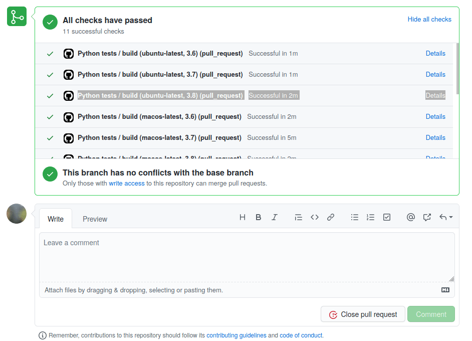
Screenshot of the GitHub checks dropdown menu[#](https://pingouin-stats.org/build/html/contributing.html#id1 "Link to this image")
* Click on the check that starts with `Python tests / build (ubuntu-latest, 3.8)`
* Now in the top right corner of the opening window, you will see a small dropdown menu called “Artifacts”

Screenshot of the GitHub build artifacts dropdown menu[#](https://pingouin-stats.org/build/html/contributing.html#id2 "Link to this image")
* Click on that drowndown menu and download the `docs-artifact` zip file
You can then unpack that zip file on your computer, enter the directory, and open the `index.html` file that you will find there. That should open the Pingouin documentation based on the changes from your Pull Request.
On this page
[Edit on GitHub](https://github.com/raphaelvallat/pingouin/edit/main/docs/contributing.rst)
---
# Guidelines — pingouin 0.5.5 documentation
[Skip to main content](https://pingouin-stats.org/build/html/guidelines.html#main-content)
Back to top
Ctrl+K
* [GitHub](https://github.com/raphaelvallat/pingouin "GitHub")
Guidelines[#](https://pingouin-stats.org/build/html/guidelines.html#guidelines "Link to this heading")
=======================================================================================================
In this page, you will find a collection of flowcharts designed to help you choose which functions of Pingouin are adequate for your analysis. Click on the desired flowchart to view a full scale image with hyperlinks to the relevant documentation.
ANOVA[#](https://pingouin-stats.org/build/html/guidelines.html#anova "Link to this heading")
---------------------------------------------------------------------------------------------

### Example code[#](https://pingouin-stats.org/build/html/guidelines.html#example-code "Link to this heading")
import pingouin as pg
\# Load an example dataset comparing pain threshold as a function of hair color
df \= pg.read\_dataset('anova')
\# 1. This is a between subject design, so the first step is to test for equality of variances
pg.homoscedasticity(data\=df, dv\='Pain threshold', group\='Hair color')
\# 2. If the groups have equal variances, we can use a regular one-way ANOVA
pg.anova(data\=df, dv\='Pain threshold', between\='Hair color')
\# 3. If there is a main effect, we can proceed to post-hoc Tukey test
pg.pairwise\_tukey(data\=df, dv\='Pain threshold', between\='Hair color')
Correlation[#](https://pingouin-stats.org/build/html/guidelines.html#correlation "Link to this heading")
---------------------------------------------------------------------------------------------------------
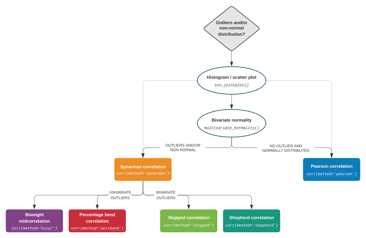
### Example code[#](https://pingouin-stats.org/build/html/guidelines.html#id2 "Link to this heading")
import pingouin as pg
import seaborn as sns
\# Load an example dataset with the personality scores of 500 participants
df \= pg.read\_dataset('pairwise\_corr')
\# 1.Test for bivariate normality (optional)
pg.multivariate\_normality(df\[\['Neuroticism', 'Openness'\]\])
\# 1bis. Visual inspection with a histogram + scatter plot (optional)
sns.jointplot(data\=df, x\='Neuroticism', y\='Openness', kind\='reg')
\# 2. If the data have a bivariate normal distribution and no clear outlier(s), we can use a regular Pearson correlation
pg.corr(df\['Neuroticism'\], df\['Openness'\], method\='pearson')
Non-parametric[#](https://pingouin-stats.org/build/html/guidelines.html#non-parametric "Link to this heading")
---------------------------------------------------------------------------------------------------------------

### Example code[#](https://pingouin-stats.org/build/html/guidelines.html#id3 "Link to this heading")
import pingouin as pg
\# Load an example dataset comparing pain threshold as a function of hair color
df \= pg.read\_dataset('anova')
\# There are 4 independent groups in our dataset, we'll therefore use the Kruskal-Wallis test:
pg.kruskal(data\=df, dv\='Pain threshold', between\='Hair color')
On this page
[Edit on GitHub](https://github.com/raphaelvallat/pingouin/edit/main/docs/guidelines.rst)
---
# FAQ — pingouin 0.5.5 documentation
[Skip to main content](https://pingouin-stats.org/build/html/faq.html#main-content)
Back to top
Ctrl+K
* [GitHub](https://github.com/raphaelvallat/pingouin "GitHub")
FAQ[#](https://pingouin-stats.org/build/html/faq.html#faq "Link to this heading")
==================================================================================
Installation[#](https://pingouin-stats.org/build/html/faq.html#installation "Link to this heading")
----------------------------------------------------------------------------------------------------
### How can I install Pingouin on my computer?[#](https://pingouin-stats.org/build/html/faq.html#how-can-i-install-pingouin-on-my-computer "Link to this heading")
To install Pingouin, open a command prompt (or Terminal or Anaconda Prompt) and type:
pip install pingouin \--upgrade
You should now be able to use Pingouin. To try it, you need to open an interactive Python console (either [IPython](https://ipython.org/)
or [Jupyter](https://jupyter.readthedocs.io/en/latest/index.html)
). For example, type the following command in a command prompt:
ipython
Now, let’s do a simple paired T-test using Pingouin:
import pingouin as pg
\# Create two variables
x \= \[4, 6, 5, 7, 6\]
y \= \[2, 2, 3, 1, 2\]
\# Run a T-test
pg.ttest(x, y, paired\=True)
### How to import and use Pingouin?[#](https://pingouin-stats.org/build/html/faq.html#how-to-import-and-use-pingouin "Link to this heading")
\# 1) Import the full package
\# --> Best if you are planning to use several Pingouin functions.
import pingouin as pg
pg.ttest(x, y)
\# 2) Import specific functions
\# --> Best if you are planning to use only this specific function.
from pingouin import ttest
ttest(x, y)
### What are the differences between statsmodels and Pingouin?[#](https://pingouin-stats.org/build/html/faq.html#what-are-the-differences-between-statsmodels-and-pingouin "Link to this heading")
[Statsmodels](https://www.statsmodels.org/stable/index.html)
is a great statistical Python package that provides several advanced functions (regression, GLM, time-series analysis) as well as an R-like syntax for fitting models. However, statsmodels can be quite hard to grasp and use for Python beginners and/or users who just want to perform simple statistical tests. The goal of Pingouin is not to replace statsmodels but rather to provide some easy-to-use functions to perform the most widely-used statistical tests. In addition, Pingouin also provides some novel functions (to cite but a few: effect sizes, pairwise T-tests and correlations, ICC, repeated measures correlation, circular statistics…).
### What are the differences between scipy.stats and Pingouin?[#](https://pingouin-stats.org/build/html/faq.html#what-are-the-differences-between-scipy-stats-and-pingouin "Link to this heading")
The [scipy.stats](https://docs.scipy.org/doc/scipy/reference/stats.html)
module provides several low-level statistical functions. However, most of these functions do not return a very detailed output (e.g. only the T- and p-values for a T-test). Most Pingouin functions are using the low-level SciPy funtions to provide a richer, more exhaustive, output. See for yourself!:
import pingouin as pg
from scipy.stats import ttest\_ind
x \= \[4, 6, 5, 7, 6\]
y \= \[2, 2, 3, 1, 2\]
print(pg.ttest(x, y)) \# Pingouin: returns a DataFrame with T-value, p-value, degrees of freedom, tail, Cohen d, power and Bayes Factor
print(ttest\_ind(x, y)) \# SciPy: returns only the T- and p-values
Data[#](https://pingouin-stats.org/build/html/faq.html#data "Link to this heading")
------------------------------------------------------------------------------------
### How can I load a .csv or .xlsx file in Python?[#](https://pingouin-stats.org/build/html/faq.html#how-can-i-load-a-csv-or-xlsx-file-in-python "Link to this heading")
You need to use the [`pandas.read_csv()`](https://pandas.pydata.org/pandas-docs/stable/reference/api/pandas.read_csv.html#pandas.read_csv "(in pandas v2.2.2)")
or [`pandas.read_excel()`](https://pandas.pydata.org/pandas-docs/stable/reference/api/pandas.read_excel.html#pandas.read_excel "(in pandas v2.2.2)")
functions:
import pandas as pd
pd.read\_csv('myfile.csv') \# Load a .csv file
pd.read\_excel('myfile.xlsx') \# Load an Excel file
### How does Pingouin deal with missing values?[#](https://pingouin-stats.org/build/html/faq.html#how-does-pingouin-deal-with-missing-values "Link to this heading")
Pingouin hates missing values as much as you do!
Most functions of Pingouin will automatically remove the missing values. In the case of paired measurements (e.g. paired T-test, correlation, or repeated measures ANOVA), a listwise deletion of missing values is performed, meaning that the entire row is removed. This is generally the best strategy if you have a large sample size and only a few missing values. However, this can be quite drastic if there are a lot of missing values in your data. In that case, it might be useful to look at [imputation methods (see Pandas documentation)](https://pandas.pydata.org/pandas-docs/stable/user_guide/missing_data.html)
, or use a linear mixed effect model instead, which natively supports missing values. However, the latter is not implemented in Pingouin.
### What’s the difference between wide format and long format data and how can I convert my data from one to the other?[#](https://pingouin-stats.org/build/html/faq.html#what-s-the-difference-between-wide-format-and-long-format-data-and-how-can-i-convert-my-data-from-one-to-the-other "Link to this heading")
In wide format, each row represent a subject, and each column a measurement (e.g. “Pre”, “Post”). This is the most convenient way for humans to look at repeated measurements. It typically results in spreadsheet with a larger number of columns than rows. An example of wide-format dataframe is shown below:
| Subject | Pre | Post | Gender | Age |
| --- | --- | --- | --- | --- |
| 1 | 2.5 | 3.1 | M | 24 |
| 2 | 4.2 | 4.8 | F | 32 |
| 3 | 2.5 | 2.9 | F | 38 |
In long-format, each row is one time point per subject and each column is a variable (e.g. one column with the “Subject” identifier, another with the “Scores” and another with the “Time” grouping factors). In long-format, there are usually many more rows than columns. While this is harder to read for humans, this is much easier to read for computers. For this reason, all the repeated measures functions in Pingouin work only with long-format dataframe. In the example below, the wide-format dataframe from above was converted into a long-format dataframe:
| Subject | Gender | Age | Time | Scores |
| --- | --- | --- | --- | --- |
| 1 | M | 24 | Pre | 2.5 |
| 1 | M | 24 | Post | 3.1 |
| 2 | F | 32 | Pre | 4.2 |
| 2 | F | 32 | Post | 4.8 |
| 3 | F | 38 | Pre | 2.5 |
| 3 | F | 38 | Post | 2.9 |
The [Pandas](https://pandas.pydata.org/)
package provides some convenient functions to convert from one format to the other:
* From wide-format to long-format (easier to read for computer), use the [`pandas.melt()`](https://pandas.pydata.org/pandas-docs/stable/reference/api/pandas.melt.html#pandas.melt "(in pandas v2.2.2)")
function.
* From long-format to wide-format, use the [`pandas.pivot_table()`](https://pandas.pydata.org/pandas-docs/stable/reference/api/pandas.pivot_table.html#pandas.pivot_table "(in pandas v2.2.2)")
function.
### Can I compute descriptive statistics with Pingouin?[#](https://pingouin-stats.org/build/html/faq.html#can-i-compute-descriptive-statistics-with-pingouin "Link to this heading")
No, the central idea behind Pingouin is that all data manipulations and descriptive statistics should be first performed in Pandas (or NumPy). For example, to compute the mean, standard deviation, and quartiles of all the numeric columns of a pandas DataFrame, one can easily use the [`pandas.DataFrame.describe()`](https://pandas.pydata.org/pandas-docs/stable/reference/api/pandas.DataFrame.describe.html#pandas.DataFrame.describe "(in pandas v2.2.2)")
method:
data.describe()
Others[#](https://pingouin-stats.org/build/html/faq.html#others "Link to this heading")
----------------------------------------------------------------------------------------
### Why is Pingouin licensed under the GNU-GPL v3?[#](https://pingouin-stats.org/build/html/faq.html#why-is-pingouin-licensed-under-the-gnu-gpl-v3 "Link to this heading")
Pingouin is licensed under the GNU General Public License v3.0 (GPL-3), which is less permissive than the BSD or MIT licenses. The reason for this is that Pingouin borrows extensively from R packages, which are all licensed under the GPL-3. To read more about what you can do and cannot do with a GPL-3 license, please visit [tldrlegal.com](https://tldrlegal.com/license/gnu-general-public-license-v3-(gpl-3)#summary)
or [choosealicense.com](https://choosealicense.com/licenses/)
.
### How can I be notified of new releases?[#](https://pingouin-stats.org/build/html/faq.html#how-can-i-be-notified-of-new-releases "Link to this heading")
You can click “Watch” on the [GitHub](https://github.com/raphaelvallat/pingouin)
of Pingouin:
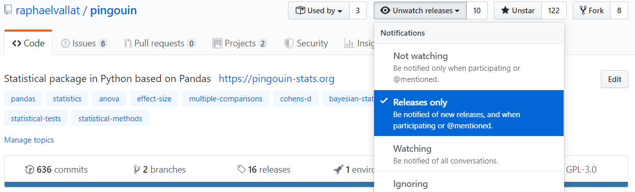
Whenever a new release is available, you can simply upgrade your version by typing the following line in a terminal window:
pip install \--upgrade pingouin
### I am not a programmer, how can I contribute to Pingouin?[#](https://pingouin-stats.org/build/html/faq.html#i-am-not-a-programmer-how-can-i-contribute-to-pingouin "Link to this heading")
There are many ways to contribute to Pingouin, even if you are not a programmer, for example, reporting bugs or results that are inconsistent with other statistical softwares, improving the documentation and examples, or, even [buying the developers a coffee](https://www.paypal.com/cgi-bin/webscr?cmd=_donations&business=K2FZVJGCKYPAG¤cy_code=USD&source=url)
!
### How can I cite Pingouin?[#](https://pingouin-stats.org/build/html/faq.html#how-can-i-cite-pingouin "Link to this heading")
Please go to [Citation and logo](https://pingouin-stats.org/build/html/citing.html#citing)
.
On this page
[Edit on GitHub](https://github.com/raphaelvallat/pingouin/edit/main/docs/faq.rst)
---
# Citation and logo — pingouin 0.5.5 documentation
[Skip to main content](https://pingouin-stats.org/build/html/citing.html#main-content)
Back to top
Ctrl+K
* [GitHub](https://github.com/raphaelvallat/pingouin "GitHub")
Citation and logo[#](https://pingouin-stats.org/build/html/citing.html#citation-and-logo "Link to this heading")
=================================================================================================================
Citing[#](https://pingouin-stats.org/build/html/citing.html#id1 "Link to this heading")
----------------------------------------------------------------------------------------
If you want to cite Pingouin, please use the publication in JOSS:
> Vallat, R. (2018). Pingouin: statistics in Python. _Journal of Open Source Software_, 3(31), 1026, [https://doi.org/10.21105/joss.01026](https://doi.org/10.21105/joss.01026)
Here is a ready-made BibTeX entry:
@article{Vallat2018,
title = {Pingouin: statistics in Python},
volume = {3},
DOI = {10.21105/joss.01026},
number = {31},
journal = {Journal of Open Source Software},
publisher = {The Open Journal},
author = {Vallat, Raphael},
year = {2018},
month = nov,
pages = {1026}
}
Logo[#](https://pingouin-stats.org/build/html/citing.html#logo "Link to this heading")
---------------------------------------------------------------------------------------
### Wide logo[#](https://pingouin-stats.org/build/html/citing.html#wide-logo "Link to this heading")

### Quadratic logo[#](https://pingouin-stats.org/build/html/citing.html#quadratic-logo "Link to this heading")

On this page
[Edit on GitHub](https://github.com/raphaelvallat/pingouin/edit/main/docs/citing.rst)
---
# What’s new — pingouin 0.5.5 documentation
[Skip to main content](https://pingouin-stats.org/build/html/changelog.html#main-content)
Back to top
Ctrl+K
* [GitHub](https://github.com/raphaelvallat/pingouin "GitHub")
What’s new[#](https://pingouin-stats.org/build/html/changelog.html#what-s-new "Link to this heading")
======================================================================================================
v0.5.5 (September 2024)[#](https://pingouin-stats.org/build/html/changelog.html#v0-5-5-september-2024 "Link to this heading")
------------------------------------------------------------------------------------------------------------------------------
This is a minor release with several bugfixes, and major updates to the internal structure and sphinx documentation.
See the full [changelog for 0.5.5](https://github.com/raphaelvallat/pingouin/releases/tag/v0.5.5)
.
v0.5.4 (January 2024)[#](https://pingouin-stats.org/build/html/changelog.html#v0-5-4-january-2024 "Link to this heading")
--------------------------------------------------------------------------------------------------------------------------
This is a minor release with several bugfixes and no new features. The new version is tested for Python 3.8-3.11 (but should also work with Python 3.12). See the full [changelog for 0.5.4](https://github.com/raphaelvallat/pingouin/releases/tag/v0.5.4)
.
This release requires pandas≥1.5. We recommend scipy≥1.11.0.
* * *
v0.5.3 (December 2022)[#](https://pingouin-stats.org/build/html/changelog.html#v0-5-3-december-2022 "Link to this heading")
----------------------------------------------------------------------------------------------------------------------------
**Bugfixes**
* Fixed a bug where the boolean value returned by [`pingouin.anderson()`](https://pingouin-stats.org/build/html/generated/pingouin.anderson.html#pingouin.anderson "pingouin.anderson")
was inverted. It returned True when the data was NOT coming from the tested distribution, and vice versa. [PR 308](https://github.com/raphaelvallat/pingouin/pull/308)
.
* Fixed misleading documentation and `input_type` in the [`pingouin.convert_effsize()`](https://pingouin-stats.org/build/html/generated/pingouin.convert_effsize.html#pingouin.convert_effsize "pingouin.convert_effsize")
function. When converting from a Cohen’s d effect size to a correlation coefficient, the resulting correlation is **not** a Pearson correlation but instead a [point-biserial correlation](https://en.wikipedia.org/wiki/Point-biserial_correlation_coefficient)
. To avoid any confusion, `input_type='r'` has been deprecated and replaced with `input_type='pointbiserialr'`. For more details, see [issue 302](https://github.com/raphaelvallat/pingouin/issues/302)
.
**New function**
We have added the [`pingouin.ptests()`](https://pingouin-stats.org/build/html/generated/pingouin.ptests.html#pingouin.ptests "pingouin.ptests")
function to calculate a T-test (T- and p-values) between all pairs of columns in a given dataframe. This is the T-test equivalent of [`pingouin.rcorr()`](https://pingouin-stats.org/build/html/generated/pingouin.rcorr.html#pingouin.rcorr "pingouin.rcorr")
. It can only be used as a [`pandas.DataFrame`](https://pandas.pydata.org/pandas-docs/stable/reference/api/pandas.DataFrame.html#pandas.DataFrame "(in pandas v2.2.2)")
method, not as a standalone function. The output is a square dataframe with the T-values on the lower triangle and the p-values on the upper triangle.
\>>> import pingouin as pg
\>>> df \= pg.read\_dataset('pairwise\_corr').iloc\[:30, 1:\]
\>>> df.columns \= \["N", "E", "O", "A", "C"\]
\>>> df.ptests()
N E O A C
N - \*\*\* \*\*\* \*\*\* \*\*\*
E -8.397 - \*\*\*
O -8.585 -0.483 - \*\*\*
A -9.026 0.278 0.786 - \*\*\*
C -4.759 3.753 4.128 3.802 -
**Improvements**
* Effect sizes are now calculated using an exact method instead of an approximation based on T-values in [`pingouin.pairwise_tukey()`](https://pingouin-stats.org/build/html/generated/pingouin.pairwise_tukey.html#pingouin.pairwise_tukey "pingouin.pairwise_tukey")
and [`pingouin.pairwise_gameshowell()`](https://pingouin-stats.org/build/html/generated/pingouin.pairwise_gameshowell.html#pingouin.pairwise_gameshowell "pingouin.pairwise_gameshowell")
. [PR 328](https://github.com/raphaelvallat/pingouin/pull/328)
.
* [`pingouin.normality()`](https://pingouin-stats.org/build/html/generated/pingouin.normality.html#pingouin.normality "pingouin.normality")
does not raise an AssertionError anymore if one of the groups in `group` has ≤ 3 samples. [PR 324](https://github.com/raphaelvallat/pingouin/pull/324)
.
* Added customization options to [`pingouin.plot_rm_corr()`](https://pingouin-stats.org/build/html/generated/pingouin.plot_rm_corr.html#pingouin.plot_rm_corr "pingouin.plot_rm_corr")
, which now takes optional keyword arguments to pass through to [`seaborn.regplot()`](https://seaborn.pydata.org/generated/seaborn.regplot.html#seaborn.regplot "(in seaborn v0.13.2)")
and [`seaborn.scatterplot()`](https://seaborn.pydata.org/generated/seaborn.scatterplot.html#seaborn.scatterplot "(in seaborn v0.13.2)")
. [PR 312](https://github.com/raphaelvallat/pingouin/pull/312)
.
* Changed some plotting functions to increase compatibility with [`seaborn.FacetGrid`](https://seaborn.pydata.org/generated/seaborn.FacetGrid.html#seaborn.FacetGrid "(in seaborn v0.13.2)")
. As explained in [issue 306](https://github.com/raphaelvallat/pingouin/issues/306)
, the major change is to generate matplotlib.axes using default parameters instead of accepting `fig` and `dpi` keyword arguments. This change applies to [`pingouin.plot_blandaltman()`](https://pingouin-stats.org/build/html/generated/pingouin.plot_blandaltman.html#pingouin.plot_blandaltman "pingouin.plot_blandaltman")
, [`pingouin.plot_paired()`](https://pingouin-stats.org/build/html/generated/pingouin.plot_paired.html#pingouin.plot_paired "pingouin.plot_paired")
, [`pingouin.plot_circmean()`](https://pingouin-stats.org/build/html/generated/pingouin.plot_circmean.html#pingouin.plot_circmean "pingouin.plot_circmean")
, and [`pingouin.qqplot()`](https://pingouin-stats.org/build/html/generated/pingouin.qqplot.html#pingouin.qqplot "pingouin.qqplot")
. In the future, open a matplotlib.axes and pass it through using the `ax` parameter to use custom figure settings with these functions. Other minor changes include the addition of the `square` keyword argument to [`pingouin.plot_circmean()`](https://pingouin-stats.org/build/html/generated/pingouin.plot_circmean.html#pingouin.plot_circmean "pingouin.plot_circmean")
and [`pingouin.qqplot()`](https://pingouin-stats.org/build/html/generated/pingouin.qqplot.html#pingouin.qqplot "pingouin.qqplot")
to ensure equal aspect ratios, and the removal of `scatter_kws` as a keyword argument in `pingouin.plot_blandaltmann()` (now alter the scatter parameters using general `**kwargs`). [PR 314](https://github.com/raphaelvallat/pingouin/pull/314)
.
* * *
v0.5.2 (June 2022)[#](https://pingouin-stats.org/build/html/changelog.html#v0-5-2-june-2022 "Link to this heading")
--------------------------------------------------------------------------------------------------------------------
**Bugfixes**
1. The eta-squared (`n2`) effect size was not properly calculated in one-way and two-way repeated measures ANOVAs. Specifically, Pingouin followed the same behavior as JASP, i.e. the eta-squared was the same as the partial eta-squared. However, as explained in [issue 251](https://github.com/raphaelvallat/pingouin/issues/251)
, this behavior is not valid. In one-way ANOVA design, the eta-squared should be equal to the generalized eta-squared. Note that, as of March 2022, this bug is also present in JASP. We have therefore updated the unit tests to use JAMOVI instead.
Warning
Please double check any effect sizes previously obtained with the [`pingouin.rm_anova()`](https://pingouin-stats.org/build/html/generated/pingouin.rm_anova.html#pingouin.rm_anova "pingouin.rm_anova")
function.
2. Fixed invalid resampling behavior for bivariate functions in [`pingouin.compute_bootci()`](https://pingouin-stats.org/build/html/generated/pingouin.compute_bootci.html#pingouin.compute_bootci "pingouin.compute_bootci")
when x and y were not paired. [PR 281](https://github.com/raphaelvallat/pingouin/pull/281)
.
3. Fixed bug where `confidence` (previously `ci`) was ignored when calculating the bootstrapped confidence intervals in [`pingouin.plot_shift()`](https://pingouin-stats.org/build/html/generated/pingouin.plot_shift.html#pingouin.plot_shift "pingouin.plot_shift")
. [PR 282](https://github.com/raphaelvallat/pingouin/pull/282)
.
**Enhancements**
1. The `pingouin.pairwise_ttests()` has been renamed to [`pingouin.pairwise_tests()`](https://pingouin-stats.org/build/html/generated/pingouin.pairwise_tests.html#pingouin.pairwise_tests "pingouin.pairwise_tests")
. Non-parametric tests are also supported in this function with the parametric=False argument, and thus the name “ttests” was misleading (see [issue 209](https://github.com/raphaelvallat/pingouin/issues/209)
).
2. Allow [`pingouin.bayesfactor_binom()`](https://pingouin-stats.org/build/html/generated/pingouin.bayesfactor_binom.html#pingouin.bayesfactor_binom "pingouin.bayesfactor_binom")
to take Beta alternative model. [PR 252](https://github.com/raphaelvallat/pingouin/pull/252)
.
3. Allow keyword arguments for logistic regression in [`pingouin.mediation_analysis()`](https://pingouin-stats.org/build/html/generated/pingouin.mediation_analysis.html#pingouin.mediation_analysis "pingouin.mediation_analysis")
. [PR 245](https://github.com/raphaelvallat/pingouin/pull/245)
.
4. Speed improvements for the Holm and FDR correction in [`pingouin.multicomp()`](https://pingouin-stats.org/build/html/generated/pingouin.multicomp.html#pingouin.multicomp "pingouin.multicomp")
. [PR 271](https://github.com/raphaelvallat/pingouin/pull/271)
.
5. Speed improvements univariate functions in [`pingouin.compute_bootci()`](https://pingouin-stats.org/build/html/generated/pingouin.compute_bootci.html#pingouin.compute_bootci "pingouin.compute_bootci")
(e.g. `func="mean"` is now vectorized).
6. Rename `eta` to `eta_squared` in [`pingouin.power_anova()`](https://pingouin-stats.org/build/html/generated/pingouin.power_anova.html#pingouin.power_anova "pingouin.power_anova")
and [`pingouin.power_rm_anova()`](https://pingouin-stats.org/build/html/generated/pingouin.power_rm_anova.html#pingouin.power_rm_anova "pingouin.power_rm_anova")
to avoid any confusion. [PR 280](https://github.com/raphaelvallat/pingouin/pull/280)
.
7. Use [black](https://black.readthedocs.io/en/stable/)
code formatting.
8. Add support for [DataMatrix](https://pydatamatrix.eu/)
objects. [PR 286](https://github.com/raphaelvallat/pingouin/pull/286)
.
**Dependencies**
1. Force scikit-learn<1.1.0 to avoid bug in [`pingouin.logistic_regression()`](https://pingouin-stats.org/build/html/generated/pingouin.logistic_regression.html#pingouin.logistic_regression "pingouin.logistic_regression")
. [PR 272](https://github.com/raphaelvallat/pingouin/issues/272)
.
* * *
v0.5.1 (February 2022)[#](https://pingouin-stats.org/build/html/changelog.html#v0-5-1-february-2022 "Link to this heading")
----------------------------------------------------------------------------------------------------------------------------
This is a minor release, with several bugfixes and improvements. This release is compatible with SciPy 1.8 and Pandas 1.4.
**Bugfixes**
1. Added support for SciPy 1.8 and Pandas 1.4. [PR 234](https://github.com/raphaelvallat/pingouin/pull/234)
.
2. Fixed bug where [`pingouin.rm_anova()`](https://pingouin-stats.org/build/html/generated/pingouin.rm_anova.html#pingouin.rm_anova "pingouin.rm_anova")
and [`pingouin.mixed_anova()`](https://pingouin-stats.org/build/html/generated/pingouin.mixed_anova.html#pingouin.mixed_anova "pingouin.mixed_anova")
changed the dtypes of categorical columns in-place ([issue 224](https://github.com/raphaelvallat/pingouin/issues/224)
).
**Enhancements**
1. Faster implementation of [`pingouin.gzscore()`](https://pingouin-stats.org/build/html/generated/pingouin.gzscore.html#pingouin.gzscore "pingouin.gzscore")
, adding all options available in zscore: axis, ddof and nan\_policy. Warning: this functions is deprecated and will be removed in pingouin 0.7.0 (use [`scipy.stats.gzscore()`](https://docs.scipy.org/doc/scipy/reference/generated/scipy.stats.gzscore.html#scipy.stats.gzscore "(in SciPy v1.14.1)")
instead). [PR 210](https://github.com/raphaelvallat/pingouin/pull/210)
.
2. Replace use of statsmodels’ studentized range distribution functions with more SciPy’s more accurate `scipy.stats.studentized_range()`. [PR 229](https://github.com/raphaelvallat/pingouin/pull/229)
.
3. Add support for optional keywords argument in the [`pingouin.homoscedasticity()`](https://pingouin-stats.org/build/html/generated/pingouin.homoscedasticity.html#pingouin.homoscedasticity "pingouin.homoscedasticity")
function ([issue 218](https://github.com/raphaelvallat/pingouin/issues/218)
).
4. Add support for the Jarque-Bera test in [`pingouin.normality()`](https://pingouin-stats.org/build/html/generated/pingouin.normality.html#pingouin.normality "pingouin.normality")
([issue 216](https://github.com/raphaelvallat/pingouin/issues/216)
).
Lastly, we have also deprecated the Gitter forum in favor of [GitHub Discussions](https://github.com/raphaelvallat/pingouin/discussions)
. Please use Discussions to ask questions, share ideas / tips and engage with the Pingouin community!
* * *
v0.5.0 (October 2021)[#](https://pingouin-stats.org/build/html/changelog.html#v0-5-0-october-2021 "Link to this heading")
--------------------------------------------------------------------------------------------------------------------------
This is a MAJOR RELEASE with several important bugfixes. We recommend all users to upgrade to this new version.
**BUGFIX - Repeated measurements**
This release fixes several critical issues related to how Pingouin handles missing values in repeated measurements. The following functions have been corrected:
* [`pingouin.rm_anova()`](https://pingouin-stats.org/build/html/generated/pingouin.rm_anova.html#pingouin.rm_anova "pingouin.rm_anova")
* [`pingouin.mixed_anova()`](https://pingouin-stats.org/build/html/generated/pingouin.mixed_anova.html#pingouin.mixed_anova "pingouin.mixed_anova")
* `pingouin.pairwise_ttests()`, only for mixed design or two-way repeated measures design.
A full description of the issue, with code and example, can be found at: [raphaelvallat/pingouin#206](https://github.com/raphaelvallat/pingouin/issues/206)
. In short, in Pingouin <0.5.0, listwise deletion of subjects (or rows) with missing values was not strictly enforced in repeated measures or mixed ANOVA, depending on the input data format (if missing values were explicit or implicit). Pingouin 0.5.0 now uses a stricter complete-case analysis regardless of the input data format, which is the same behavior as JASP.
Furthermore, the `pingouin.remove_rm_na()` has been deprecated. Instead, listwise deletion of rows with missing values in repeated measurements is now performed using:
\>>> data\_piv \= data.pivot\_table(index\=subject, columns\=within, values\=dv)
\>>> data\_piv \= data\_piv.dropna() \# Listwise deletion
\>>> data \= data\_piv.melt(ignore\_index\=False, value\_name\=dv).reset\_index()
**BUGFIX - Strict listwise deletion in pairwise\_ttests when repeated measures are present**
This is related to the previous issue. In mixed design, listwise deletion (complete-case analysis) was not strictly enforced in `pingouin.pairwise_ttests()` for the between-subject and interaction T-tests. In other words, the between-subject and interaction T-tests were calculated using a pairwise-deletion approach, even with `nan_policy="pairwise"`. The same issue occured in two-way repeated measures design, in which no strict listwise deletion was performed prior to calculating the T-tests, even with `nan_policy="pairwise"`.
This has now been fixed such that Pingouin will always perform a strict listwise deletion whenever repeated measurements are present when `nan_policy="listwise"` (default). This complete-case analysis behavior can be disabled with `nan_policy="pairwise"`, in which case missing values will be removed separately for each contrast. This may not be appropriate for post-hoc analysis following a repeated measures or mixed ANOVA, which is always conducted on complete-case data.
**BUGFIX - Homoscedasticity**
The [`pingouin.homoscedasticity()`](https://pingouin-stats.org/build/html/generated/pingouin.homoscedasticity.html#pingouin.homoscedasticity "pingouin.homoscedasticity")
gave WRONG results for wide-format dataframes because the test was incorrectly calculated on the transposed data. See [issue 204](https://github.com/raphaelvallat/pingouin/issues/204)
.
**Enhancements**
1. Partial correlation functions ([`pingouin.pcorr()`](https://pingouin-stats.org/build/html/generated/pingouin.pcorr.html#pingouin.pcorr "pingouin.pcorr")
and [`pingouin.partial_corr()`](https://pingouin-stats.org/build/html/generated/pingouin.partial_corr.html#pingouin.partial_corr "pingouin.partial_corr")
) now use [`numpy.linalg.pinv()`](https://numpy.org/doc/stable/reference/generated/numpy.linalg.pinv.html#numpy.linalg.pinv "(in NumPy v2.1)")
with hermitian=True, which improves numerical stability. See [issue 198](https://github.com/raphaelvallat/pingouin/issues/198)
.
2. Added support for integer column names in most functions. Previously, Pingouin raised an error if the column names were integers. See [issue 201](https://github.com/raphaelvallat/pingouin/issues/201)
.
3. [`pingouin.pairwise_corr()`](https://pingouin-stats.org/build/html/generated/pingouin.pairwise_corr.html#pingouin.pairwise_corr "pingouin.pairwise_corr")
now works when the column names of the dataframe are integer, and better support numpy.arrays in the `columns` argument.
4. Added support for wide-format dataframe in [`pingouin.friedman()`](https://pingouin-stats.org/build/html/generated/pingouin.friedman.html#pingouin.friedman "pingouin.friedman")
and [`pingouin.cochran()`](https://pingouin-stats.org/build/html/generated/pingouin.cochran.html#pingouin.cochran "pingouin.cochran")
* * *
v0.4.0 (August 2021)[#](https://pingouin-stats.org/build/html/changelog.html#v0-4-0-august-2021 "Link to this heading")
------------------------------------------------------------------------------------------------------------------------
Major upgrade of the dependencies. This release requires **Python 3.7+, SciPy 1.7+, NumPy 1.19+ and Pandas 1.0+**. Pingouin uses the `alternative` argument that has been added to several statistical functions of Scipy 1.7+ (see below). However, SciPy 1.7+ requires Python 3.7+. We recommend all users to upgrade to the latest version of Pingouin.
### Major enhancements[#](https://pingouin-stats.org/build/html/changelog.html#major-enhancements "Link to this heading")
**Directional testing**
The `tail` argument has been renamed to `alternative` in all Pingouin functions to be consistent with SciPy and R ([#185](https://github.com/raphaelvallat/pingouin/issues/185)
). Furthermore, `"alternative='one-sided'"` has now been deprecated. Instead, `alternative` must be one of “two-sided” (default), “greater” or “less”. Again, this is the same behavior as SciPy and R.
Added support for directional testing with `"alternative='greater'"` and `"alternative='less'"` in [`pingouin.corr()`](https://pingouin-stats.org/build/html/generated/pingouin.corr.html#pingouin.corr "pingouin.corr")
([#176](https://github.com/raphaelvallat/pingouin/issues/176)
). As a result, the p-value, confidence intervals and power of the correlation will change depending on the directionality of the test. Support for directional testing has also been added to [`pingouin.power_corr()`](https://pingouin-stats.org/build/html/generated/pingouin.power_corr.html#pingouin.power_corr "pingouin.power_corr")
and [`pingouin.compute_esci()`](https://pingouin-stats.org/build/html/generated/pingouin.compute_esci.html#pingouin.compute_esci "pingouin.compute_esci")
.
Finally, the `tail` argument has been removed from [`pingouin.rm_corr()`](https://pingouin-stats.org/build/html/generated/pingouin.rm_corr.html#pingouin.rm_corr "pingouin.rm_corr")
, [`pingouin.circ_corrcc()`](https://pingouin-stats.org/build/html/generated/pingouin.circ_corrcc.html#pingouin.circ_corrcc "pingouin.circ_corrcc")
and [`pingouin.circ_corrcl()`](https://pingouin-stats.org/build/html/generated/pingouin.circ_corrcl.html#pingouin.circ_corrcl "pingouin.circ_corrcl")
to be consistent with the original R / Matlab implementations.
**Partial correlation**
Major refactoring of [`pingouin.partial_corr()`](https://pingouin-stats.org/build/html/generated/pingouin.partial_corr.html#pingouin.partial_corr "pingouin.partial_corr")
, which now uses the same method as the R [ppcor](https://cran.r-project.org/web/packages/ppcor/ppcor.pdf)
package, i.e. based on the inverse covariance matrix rather than the residuals of a linear regression. This new approach is faster and works better in some cases (such as Spearman partial correlation with binary variables, see [issue 147](https://github.com/raphaelvallat/pingouin/issues/147)
). One caveat is that only the Pearson and Spearman correlation methods are now supported in partial/semi-partial correlation.
**Box M test**
Added the [`pingouin.box_m()`](https://pingouin-stats.org/build/html/generated/pingouin.box_m.html#pingouin.box_m "pingouin.box_m")
function to calculate [Box’s M test](https://en.wikipedia.org/wiki/Box%27s_M_test)
for equality of covariance matrices ([#175](https://github.com/raphaelvallat/pingouin/pull/175)
).
### Minor enhancements[#](https://pingouin-stats.org/build/html/changelog.html#minor-enhancements "Link to this heading")
* [`pingouin.wilcoxon()`](https://pingouin-stats.org/build/html/generated/pingouin.wilcoxon.html#pingouin.wilcoxon "pingouin.wilcoxon")
now supports a pre-computed array of differences, similar to [`scipy.stats.wilcoxon()`](https://docs.scipy.org/doc/scipy/reference/generated/scipy.stats.wilcoxon.html#scipy.stats.wilcoxon "(in SciPy v1.14.1)")
([issue 186](https://github.com/raphaelvallat/pingouin/issues/186)
).
* [`pingouin.mwu()`](https://pingouin-stats.org/build/html/generated/pingouin.mwu.html#pingouin.mwu "pingouin.mwu")
and [`pingouin.wilcoxon()`](https://pingouin-stats.org/build/html/generated/pingouin.wilcoxon.html#pingouin.wilcoxon "pingouin.wilcoxon")
now support keywords arguments that are passed to the lower-level scipy functions.
* Added warning in [`pingouin.partial_corr()`](https://pingouin-stats.org/build/html/generated/pingouin.partial_corr.html#pingouin.partial_corr "pingouin.partial_corr")
with `method="skipped"`: the MCD algorithm does not give the same output in Python (scikit-learn) than in the original Matlab library (LIBRA), and this can lead to skipped correlations that are different in Pingouin than in the Matlab robust correlation toolbox (see [issue 164](https://github.com/raphaelvallat/pingouin/issues/164)
).
* [`pingouin.ancova()`](https://pingouin-stats.org/build/html/generated/pingouin.ancova.html#pingouin.ancova "pingouin.ancova")
always uses statsmodels, regardless of the number of covariates. This fixes LinAlg errors in [`pingouin.ancova()`](https://pingouin-stats.org/build/html/generated/pingouin.ancova.html#pingouin.ancova "pingouin.ancova")
and [`pingouin.rm_corr()`](https://pingouin-stats.org/build/html/generated/pingouin.rm_corr.html#pingouin.rm_corr "pingouin.rm_corr")
(see [issue 184](https://github.com/raphaelvallat/pingouin/issues/184)
).
* Avoid RuntimeWarning when calculating CI and power of a perfect correlation in [`pingouin.corr()`](https://pingouin-stats.org/build/html/generated/pingouin.corr.html#pingouin.corr "pingouin.corr")
(see [issue 183](https://github.com/raphaelvallat/pingouin/issues/183)
).
* Use [`scipy.linalg.lstsq()`](https://docs.scipy.org/doc/scipy/reference/generated/scipy.linalg.lstsq.html#scipy.linalg.lstsq "(in SciPy v1.14.1)")
instead of [`numpy.linalg.lstsq()`](https://numpy.org/doc/stable/reference/generated/numpy.linalg.lstsq.html#numpy.linalg.lstsq "(in NumPy v2.1)")
whenever possible to better check for NaN and Inf in input (see [issue 184](https://github.com/raphaelvallat/pingouin/issues/184)
).
* flake8 requirements for max line length has been changed from 80 to 100 characters.
* * *
v0.3.12 (May 2021)[#](https://pingouin-stats.org/build/html/changelog.html#v0-3-12-may-2021 "Link to this heading")
--------------------------------------------------------------------------------------------------------------------
**Bugfixes**
This release fixes a critical error in [`pingouin.partial_corr()`](https://pingouin-stats.org/build/html/generated/pingouin.partial_corr.html#pingouin.partial_corr "pingouin.partial_corr")
: the number of covariates was not taken into account when calculating the degrees of freedom of the partial correlation, thus leading to incorrect results (except for the correlation coefficient which remained unaffected). For more details, please see [issue 171](https://github.com/raphaelvallat/pingouin/issues/171)
.
In addition to fixing the p-values and 95% confidence intervals, the statistical power and Bayes Factor have been removed from the output of [`pingouin.partial_corr()`](https://pingouin-stats.org/build/html/generated/pingouin.partial_corr.html#pingouin.partial_corr "pingouin.partial_corr")
, at least temporary until we can make sure that these give exact results.
We have also fixed a minor bug in the robust skipped and shepherd correlation (see [`pingouin.corr()`](https://pingouin-stats.org/build/html/generated/pingouin.corr.html#pingouin.corr "pingouin.corr")
), for which the calculation of the confidence intervals and statistical power did not take into account the number of outliers. These are now calculated only on the cleaned data.
Warning
We therefore strongly recommend that all users UPDATE Pingouin (`pip install -U pingouin`) and CHECK ANY RESULTS obtained with the [`pingouin.partial_corr()`](https://pingouin-stats.org/build/html/generated/pingouin.partial_corr.html#pingouin.partial_corr "pingouin.partial_corr")
function.
**Enhancements**
1. Major refactoring of [`pingouin.plot_blandaltman()`](https://pingouin-stats.org/build/html/generated/pingouin.plot_blandaltman.html#pingouin.plot_blandaltman "pingouin.plot_blandaltman")
, which now has many additional parameters. It also uses a T distribution instead of a normal distribution to estimate the 95% confidence intervals of the mean difference and agreement limits. See [issue 167](https://github.com/raphaelvallat/pingouin/issues/167)
.
2. For clarity, the z, r2 and adj\_r2 have been removed from the output of [`pingouin.corr()`](https://pingouin-stats.org/build/html/generated/pingouin.corr.html#pingouin.corr "pingouin.corr")
and [`pingouin.pairwise_corr()`](https://pingouin-stats.org/build/html/generated/pingouin.pairwise_corr.html#pingouin.pairwise_corr "pingouin.pairwise_corr")
, as these can be readily calculated from the correlation coefficient.
3. Better testing against R for [`pingouin.partial_corr()`](https://pingouin-stats.org/build/html/generated/pingouin.partial_corr.html#pingouin.partial_corr "pingouin.partial_corr")
and [`pingouin.corr()`](https://pingouin-stats.org/build/html/generated/pingouin.corr.html#pingouin.corr "pingouin.corr")
.
v0.3.11 (April 2021)[#](https://pingouin-stats.org/build/html/changelog.html#v0-3-11-april-2021 "Link to this heading")
------------------------------------------------------------------------------------------------------------------------
**Bugfixes**
1. Fix invalid computation of the robust skipped correlation in [`pingouin.corr()`](https://pingouin-stats.org/build/html/generated/pingouin.corr.html#pingouin.corr "pingouin.corr")
(see [issue 164](https://github.com/raphaelvallat/pingouin/issues/164)
).
2. Passing a wrong `tail` argument to [`pingouin.corr()`](https://pingouin-stats.org/build/html/generated/pingouin.corr.html#pingouin.corr "pingouin.corr")
now _always_ raises an error (see [PR 160](https://github.com/raphaelvallat/pingouin/pull/160)
). In previous versions of pingouin, using any `method` other than `"pearson"` and a wrong `tail` argument such as `"two-tailed"` or `"both"` (instead of the correct `"two-sided"`) may have resulted in silently returning a one-sided p-value.
3. Reverted changes made in [`pingouin.pairwise_corr()`](https://pingouin-stats.org/build/html/generated/pingouin.pairwise_corr.html#pingouin.pairwise_corr "pingouin.pairwise_corr")
which led to Pingouin calculating the correlations between the DV columns and the covariates, thus artificially increasing the number of pairwise comparisons (see [issue 162](https://github.com/raphaelvallat/pingouin/issues/162)
).
v0.3.10 (February 2021)[#](https://pingouin-stats.org/build/html/changelog.html#v0-3-10-february-2021 "Link to this heading")
------------------------------------------------------------------------------------------------------------------------------
**Bugfix**
This release fixes an error in the calculation of the p-values in the [`pingouin.pairwise_tukey()`](https://pingouin-stats.org/build/html/generated/pingouin.pairwise_tukey.html#pingouin.pairwise_tukey "pingouin.pairwise_tukey")
and [`pingouin.pairwise_gameshowell()`](https://pingouin-stats.org/build/html/generated/pingouin.pairwise_gameshowell.html#pingouin.pairwise_gameshowell "pingouin.pairwise_gameshowell")
functions (see [PR156](https://github.com/raphaelvallat/pingouin/pull/156)
). Old versions of Pingouin used an incorrect algorithm for the studentized range approximation, which resulted in (slightly) incorrect p-values. In most cases, the error did not seem to affect the significance of the p-values. The new version of Pingouin now uses [statsmodels internal implementation](https://github.com/statsmodels/statsmodels/blob/master/statsmodels/stats/libqsturng/qsturng_.py)
of the Gleason (1999) algorithm to estimate the p-values.
Please note that the Pingouin p-values may be slightly different than R (and JASP), because it uses a different algorithm. However, this does not seem to affect the significance levels of the p-values (i.e. a p-value below 0.05 in JASP is likely to be below 0.05 in Pingouin, and vice versa).
We therefore recommend that all users UPDATE Pingouin (`pip install -U pingouin`) and CHECK ANY RESULTS obtained with the [`pingouin.pairwise_tukey()`](https://pingouin-stats.org/build/html/generated/pingouin.pairwise_tukey.html#pingouin.pairwise_tukey "pingouin.pairwise_tukey")
and [`pingouin.pairwise_gameshowell()`](https://pingouin-stats.org/build/html/generated/pingouin.pairwise_gameshowell.html#pingouin.pairwise_gameshowell "pingouin.pairwise_gameshowell")
functions.
v0.3.9 (January 2021)[#](https://pingouin-stats.org/build/html/changelog.html#v0-3-9-january-2021 "Link to this heading")
--------------------------------------------------------------------------------------------------------------------------
**Bugfix**
This release fixes a CRITICAL ERROR in the `pingouin.pairwise_ttests()` function (see [issue 151](https://github.com/raphaelvallat/pingouin/issues/151)
). The bug concerns one-way and two-way repeated measures pairwise T-tests. Until now, Pingouin implicitly assumed that the dataframe was sorted such that the ordering of the subject was the same across all repeated measurements (e.g. the third values in the repeated measurements always belonged to the same subject). This led to incorrect results when the dataframe was not sorted in such a way.
We therefore strongly recommend that all users UPDATE Pingouin (`pip install -U pingouin`) and CHECK ANY RESULTS obtained with the `pingouin.pairwise_ttests()` function. Note that the bug does not concern non-repeated measures pairwise T-test, since the ordering of the values does not matter in this case.
Furthermore, and to prevent a similar issue, we have now disabled `marginal=False` in two-way repeated measure design. As of this release, `marginal=False` will therefore only have an impact on the between-factor T-test(s) of a mixed design.
**Deprecation**
a. Removed the Glass delta effect size. Until now, Pingouin invalidly assumed that the control group was always the one with the lowest standard deviation. Since this cannot be verified, and to avoid any confusion, the Glass delta effect size has been completely removed from Pingouin. See [issue 139](https://github.com/raphaelvallat/pingouin/issues/139)
.
**Enhancements**
1. [`pingouin.plot_paired()`](https://pingouin-stats.org/build/html/generated/pingouin.plot_paired.html#pingouin.plot_paired "pingouin.plot_paired")
now supports an arbitrary number of within-levels as well as horizontal plotting. See [PR 133](https://github.com/raphaelvallat/pingouin/pull/133)
.
2. [`pingouin.linear_regression()`](https://pingouin-stats.org/build/html/generated/pingouin.linear_regression.html#pingouin.linear_regression "pingouin.linear_regression")
now handles a rank deficient design matrix X by producing a warning and trying to calculate the sum of squared residuals without relying on `np.linalg.lstsq()`. See [issue 130](https://github.com/raphaelvallat/pingouin/issues/130)
.
3. [`pingouin.friedman()`](https://pingouin-stats.org/build/html/generated/pingouin.friedman.html#pingouin.friedman "pingouin.friedman")
now has an option to choose between Chi square test or F test method.
4. Several minor improvements to the documentation and GitHub Actions. See [PR150](https://github.com/raphaelvallat/pingouin/pull/150)
.
5. Added support for `kwargs` in [`pingouin.corr()`](https://pingouin-stats.org/build/html/generated/pingouin.corr.html#pingouin.corr "pingouin.corr")
(see [issue 138](https://github.com/raphaelvallat/pingouin/issues/138)
).
6. Added `confidence` argument in [`pingouin.ttest()`](https://pingouin-stats.org/build/html/generated/pingouin.ttest.html#pingouin.ttest "pingouin.ttest")
to allow for custom CI (see [issue 152](https://github.com/raphaelvallat/pingouin/issues/152)
).
v0.3.8 (September 2020)[#](https://pingouin-stats.org/build/html/changelog.html#v0-3-8-september-2020 "Link to this heading")
------------------------------------------------------------------------------------------------------------------------------
**Bugfixes**
1. Fix a bug in in [`pingouin.ttest()`](https://pingouin-stats.org/build/html/generated/pingouin.ttest.html#pingouin.ttest "pingouin.ttest")
in which the confidence intervals for one-sample T-test with y != 0 were invalid (e.g. `pg.ttest(x=[4, 6, 7, 4], y=4)`). See [issue 119](https://github.com/raphaelvallat/pingouin/issues/119)
.
**New features**
1. Added a pingouin.options module which can be used to set default options. For example, one can set the default decimal rounding of the output dataframe, either for the entire dataframe, per column, per row, or per cell. See [PR120](https://github.com/raphaelvallat/pingouin/pull/120)
. For more details, please refer to [notebooks/06\_others.ipynb](https://github.com/raphaelvallat/pingouin/blob/master/notebooks/06_Others.ipynb)
.
import pingouin as pg
pg.options\['round'\] \= None \# Default: no rounding
pg.options\['round'\] \= 4
pg.options\['round.column.CI95%'\] \= 2
pg.options\['round.row.T-test'\] \= 2
pg.options\['round.cell.\[T-test\]x\[CI95%\]'\] \= 2
**Enhancements**
1. [`pingouin.linear_regression()`](https://pingouin-stats.org/build/html/generated/pingouin.linear_regression.html#pingouin.linear_regression "pingouin.linear_regression")
now returns the processed X and y variables (Xw and yw for WLS) and the predicted values if `as_dataframe=False`. See [issue 112](https://github.com/raphaelvallat/pingouin/issues/112)
.
2. The Common Language Effect Size (CLES) in [`pingouin.mwu()`](https://pingouin-stats.org/build/html/generated/pingouin.mwu.html#pingouin.mwu "pingouin.mwu")
is now calculated using the formula given by Vargha and Delaney 2000, which works better when ties are present in data. This is consistent with the [`pingouin.wilcoxon()`](https://pingouin-stats.org/build/html/generated/pingouin.wilcoxon.html#pingouin.wilcoxon "pingouin.wilcoxon")
and [`pingouin.compute_effsize()`](https://pingouin-stats.org/build/html/generated/pingouin.compute_effsize.html#pingouin.compute_effsize "pingouin.compute_effsize")
functions. See [issue 114](https://github.com/raphaelvallat/pingouin/issues/114)
.
3. Better handling of kwargs arguments in [`pingouin.plot_paired()`](https://pingouin-stats.org/build/html/generated/pingouin.plot_paired.html#pingouin.plot_paired "pingouin.plot_paired")
(see [PR 116](https://github.com/raphaelvallat/pingouin/pull/116)
).
4. Added `boxplot_in_front` argument to the [`pingouin.plot_paired()`](https://pingouin-stats.org/build/html/generated/pingouin.plot_paired.html#pingouin.plot_paired "pingouin.plot_paired")
. When set to True, the boxplot is displayed in front of the lines with a slight transparency. This can make the overall plot more readable when plotting data from a large number of subjects. (see [PR 117](https://github.com/raphaelvallat/pingouin/pull/117)
).
5. Better handling of Categorical columns in several functions (e.g. ANOVA). See [issue 122](https://github.com/raphaelvallat/pingouin/issues/122)
.
6. `multivariate_normality()` now also returns the test statistic. This function also comes with better unit testing against the MVN R package.
7. [`pingouin.pairwise_corr()`](https://pingouin-stats.org/build/html/generated/pingouin.pairwise_corr.html#pingouin.pairwise_corr "pingouin.pairwise_corr")
can now control for all covariates by excluding each specific set of column-combinations from the covariates to use for this combination, similar to [`pingouin.pcorr()`](https://pingouin-stats.org/build/html/generated/pingouin.pcorr.html#pingouin.pcorr "pingouin.pcorr")
. See [PR 124](https://github.com/raphaelvallat/pingouin/pull/124)
.
8. Bayes factor formatting is now handled via the options module. The default behaviour is unchanged (return as formatted string), but can easily be disabled by setting pingouin.options\[“round.column.BF10”\] = None. See [PR 126](https://github.com/raphaelvallat/pingouin/pull/126)
.
v0.3.7 (July 2020)[#](https://pingouin-stats.org/build/html/changelog.html#v0-3-7-july-2020 "Link to this heading")
--------------------------------------------------------------------------------------------------------------------
**Bugfixes**
This hotfix release brings important changes to the [`pingouin.pairwise_tukey()`](https://pingouin-stats.org/build/html/generated/pingouin.pairwise_tukey.html#pingouin.pairwise_tukey "pingouin.pairwise_tukey")
and [`pingouin.pairwise_gameshowell()`](https://pingouin-stats.org/build/html/generated/pingouin.pairwise_gameshowell.html#pingouin.pairwise_gameshowell "pingouin.pairwise_gameshowell")
functions. These two functions had been implemented soon after Pingouin’s first release and were not as tested as more recent and widely-used functions. These two functions are now validated against [JASP](https://jasp-stats.org/)
.
We strongly recommend that all users upgrade their version of Pingouin (`pip install -U pingouin`).
1. Fixed a bug in [`pingouin.pairwise_tukey()`](https://pingouin-stats.org/build/html/generated/pingouin.pairwise_tukey.html#pingouin.pairwise_tukey "pingouin.pairwise_tukey")
and [`pingouin.pairwise_gameshowell()`](https://pingouin-stats.org/build/html/generated/pingouin.pairwise_gameshowell.html#pingouin.pairwise_gameshowell "pingouin.pairwise_gameshowell")
in which the group labels (columns A and B) were incorrect when the `between` column was encoded as a [`pandas.Categorical`](https://pandas.pydata.org/pandas-docs/stable/reference/api/pandas.Categorical.html#pandas.Categorical "(in pandas v2.2.2)")
with non-alphabetical categories order. This was caused by a discrepancy in how Numpy and Pandas sorted the categories in the `between` column. For more details, please refer to [issue 111](https://github.com/raphaelvallat/pingouin/issues/111)
.
2. Fixed a bug in [`pingouin.pairwise_gameshowell()`](https://pingouin-stats.org/build/html/generated/pingouin.pairwise_gameshowell.html#pingouin.pairwise_gameshowell "pingouin.pairwise_gameshowell")
in which the reported standard errors were slightly incorrect because of a typo in the code. However, the T-values and p-values were fortunately calculated using the correct standard errors, so this bug only impacted the values in the `se` column.
3. Removed the `tail` and `alpha` argument from the in [`pingouin.pairwise_tukey()`](https://pingouin-stats.org/build/html/generated/pingouin.pairwise_tukey.html#pingouin.pairwise_tukey "pingouin.pairwise_tukey")
and [`pingouin.pairwise_gameshowell()`](https://pingouin-stats.org/build/html/generated/pingouin.pairwise_gameshowell.html#pingouin.pairwise_gameshowell "pingouin.pairwise_gameshowell")
functions to be consistent with JASP. Note that the `alpha` parameter did not have any impact. One-sided p-values were obtained by halving the two-sided p-values.
Error
Please check all previous code and results that called the [`pingouin.pairwise_tukey()`](https://pingouin-stats.org/build/html/generated/pingouin.pairwise_tukey.html#pingouin.pairwise_tukey "pingouin.pairwise_tukey")
or [`pingouin.pairwise_gameshowell()`](https://pingouin-stats.org/build/html/generated/pingouin.pairwise_gameshowell.html#pingouin.pairwise_gameshowell "pingouin.pairwise_gameshowell")
functions, especially if the `between` column was encoded as a [`pandas.Categorical`](https://pandas.pydata.org/pandas-docs/stable/reference/api/pandas.Categorical.html#pandas.Categorical "(in pandas v2.2.2)")
.
**Deprecation**
1. We have now removed the `pingouin.plot_skipped_corr()` function, as we felt that it may not be useful or relevant to many users (see [issue 105](https://github.com/raphaelvallat/pingouin/issues/105)
).
v0.3.6 (July 2020)[#](https://pingouin-stats.org/build/html/changelog.html#v0-3-6-july-2020 "Link to this heading")
--------------------------------------------------------------------------------------------------------------------
**Bugfixes**
1. Changed the default scikit-learn solver in [`pingouin.logistic_regression()`](https://pingouin-stats.org/build/html/generated/pingouin.logistic_regression.html#pingouin.logistic_regression "pingouin.logistic_regression")
from _‘lbfgs’_ to _‘newton-cg’_ in order to get results that are [always consistent with R or statsmodels](https://stats.stackexchange.com/questions/203816/logistic-regression-scikit-learn-vs-glmnet)
. Previous version of Pingouin were based on the _‘lbfgs’_ solver which internally applied a regularization of the intercept that may have led to different coefficients and p-values for the predictors of interest based on the scaling of these predictors (e.g very small or very large values). The new _‘newton-cg’_ solver is scaling-independent, i.e. no regularization is applied to the intercept and p-values are therefore unchanged with different scaling of the data. If you prefer to keep the old behavior, just use: `pingouin.logistic_regression(..., solver='lbfgs')`.
2. Fixed invalid results in [`pingouin.logistic_regression()`](https://pingouin-stats.org/build/html/generated/pingouin.logistic_regression.html#pingouin.logistic_regression "pingouin.logistic_regression")
when `fit_intercept=False` was passed as a keyword argument to scikit-learn. The standard errors and p-values were still calculated by taking into account an intercept in the model.
Warning
We highly recommend double-checking all previous code and results that called the [`pingouin.logistic_regression()`](https://pingouin-stats.org/build/html/generated/pingouin.logistic_regression.html#pingouin.logistic_regression "pingouin.logistic_regression")
function, especially if it involved non-standardized predictors and/or custom keywords arguments passed to scikit-learn.
**Enhancements**
1. Added `within_first` boolean argument to `pingouin.pairwise_ttests()`. This is useful in mixed design when one want to change the order of the interaction. The default behavior of Pingouin is to return the within \* between pairwise tests for the interaction. Using `within_first=False`, one can now return the between \* within pairwise tests. For more details, see [issue 102](https://github.com/raphaelvallat/pingouin/issues/102)
on GitHub.
2. [`pingouin.list_dataset()`](https://pingouin-stats.org/build/html/generated/pingouin.list_dataset.html#pingouin.list_dataset "pingouin.list_dataset")
now returns a dataframe instead of simply printing the output.
3. Added the Palmer Station LTER [Penguin dataset](https://github.com/allisonhorst/palmerpenguins)
, which describes the flipper length and body mass for different species of penguins. It can be loaded with `pingouin.read_dataset('penguins')`.
4. Added the [Tips dataset](https://vincentarelbundock.github.io/Rdatasets/doc/reshape2/tips.html)
. It can be loaded with `pingouin.read_dataset('tips')`.
v0.3.5 (June 2020)[#](https://pingouin-stats.org/build/html/changelog.html#v0-3-5-june-2020 "Link to this heading")
--------------------------------------------------------------------------------------------------------------------
**Enhancements**
1. Added support for weighted linear regression in [`pingouin.linear_regression()`](https://pingouin-stats.org/build/html/generated/pingouin.linear_regression.html#pingouin.linear_regression "pingouin.linear_regression")
. Users can now pass sample weights using the `weights` argument (similar to `lm(..., weights)` in R and `LinearRegression.fit(X, y, sample_weight)` in scikit-learn).
2. The \\(R^2\\) in [`pingouin.linear_regression()`](https://pingouin-stats.org/build/html/generated/pingouin.linear_regression.html#pingouin.linear_regression "pingouin.linear_regression")
is now calculated in a similar manner as statsmodels and R, which give different results as [`sklearn.metrics.r2_score()`](https://scikit-learn.org/stable/modules/generated/sklearn.metrics.r2_score.html#sklearn.metrics.r2_score "(in scikit-learn v1.5)")
when, _and only when_, no constant term (= intercept) is present in the predictor matrix. In that case, scikit-learn (and previous versions of Pingouin) uses the standard \\(R^2\\) formula, which assumes a reference model that only includes an intercept:
\\\[R^2 = 1 - \\frac{\\sum\_i (y\_i - \\hat y\_i)^2}{\\sum\_i (y\_i - \\bar y)^2}\\\]
However, statsmodels, R, and newer versions of Pingouin use a modified formula, which uses a reference model corresponding to noise only (i.e. no intercept, as explained [in this post](https://stats.stackexchange.com/questions/26176/removal-of-statistically-significant-intercept-term-increases-r2-in-linear-mo)
):
\\\[R\_0^2 = 1 - \\frac{\\sum\_i (y\_i - \\hat y\_i)^2}{\\sum\_i y\_i^2}\\\]
Note that this only affects the (rare) cases when no intercept is present in the predictor matrix. Remember that Pingouin automatically add a constant term in [`pingouin.linear_regression()`](https://pingouin-stats.org/build/html/generated/pingouin.linear_regression.html#pingouin.linear_regression "pingouin.linear_regression")
, a behavior that can be disabled using `add_intercept=False`.
3. Added support for robust [biweight midcorrelation](https://en.wikipedia.org/wiki/Biweight_midcorrelation)
(`'bicor'`) in [`pingouin.corr()`](https://pingouin-stats.org/build/html/generated/pingouin.corr.html#pingouin.corr "pingouin.corr")
and [`pingouin.pairwise_corr()`](https://pingouin-stats.org/build/html/generated/pingouin.pairwise_corr.html#pingouin.pairwise_corr "pingouin.pairwise_corr")
.
4. The Common Language Effect Size (CLES) is now calculated using the formula given by Vargha and Delaney 2000, which works better when ties are present in data.
\\\[\\text{CL} = P(X > Y) + .5 \\times P(X = Y)\\\]
This applies to the [`pingouin.wilcoxon()`](https://pingouin-stats.org/build/html/generated/pingouin.wilcoxon.html#pingouin.wilcoxon "pingouin.wilcoxon")
and [`pingouin.compute_effsize()`](https://pingouin-stats.org/build/html/generated/pingouin.compute_effsize.html#pingouin.compute_effsize "pingouin.compute_effsize")
functions. Furthermore, the CLES is now tail-sensitive in the former, but not in the latter since tail is not a valid argument. In [`pingouin.compute_effsize()`](https://pingouin-stats.org/build/html/generated/pingouin.compute_effsize.html#pingouin.compute_effsize "pingouin.compute_effsize")
, the CLES thus always corresponds to the proportion of pairs where x is _higher_ than y. For more details, please refer to [PR #94](https://github.com/raphaelvallat/pingouin/pull/94)
.
5. Confidence intervals around a Cohen d effect size are now calculated using a central T distribution instead of a standard normal distribution in the [`pingouin.compute_esci()`](https://pingouin-stats.org/build/html/generated/pingouin.compute_esci.html#pingouin.compute_esci "pingouin.compute_esci")
function. This is consistent with the effsize R package.
**Code**
1. Added support for unsigned integers in dtypes safety checks (see [issue #93](https://github.com/raphaelvallat/pingouin/issues/93)
).
v0.3.4 (May 2020)[#](https://pingouin-stats.org/build/html/changelog.html#v0-3-4-may-2020 "Link to this heading")
------------------------------------------------------------------------------------------------------------------
**Bugfixes**
1. The Cohen \\(d\_{avg}\\) for paired samples was previously calculated using eq. 10 in [Lakens 2013](https://www.frontiersin.org/articles/10.3389/fpsyg.2013.00863/full)
. However, this equation was slightly different from the original proposed by [Cumming 2012](https://books.google.com/books/about/Understanding_the_New_Statistics.html?id=AVBDYgEACAAJ)
, and Lakens has since updated the equation in his effect size conversion [spreadsheet](https://osf.io/vbdah/)
. Pingouin now uses the correct formula, which is \\(d\_{avg} = \\frac{\\overline{X} - \\overline{Y}}{\\sqrt{\\frac{(\\sigma\_1^2 + \\sigma\_2^2)}{2}}}\\).
2. Fixed minor bug in internal function _pingouin.utils.\_flatten\_list_ that could lead to TypeError in `pingouin.pairwise_ttests()` with within/between factors encoded as integers (see [issue #91](https://github.com/raphaelvallat/pingouin/issues/91)
).
**New functions**
1. Added [`pingouin.convert_angles()`](https://pingouin-stats.org/build/html/generated/pingouin.convert_angles.html#pingouin.convert_angles "pingouin.convert_angles")
function to convert circular data in arbitrary units to radians (\\(\[-\\pi, \\pi)\\) range).\
\
\
**Enhancements**\
\
1. Better documentation and testing for descriptive circular statistics functions.\
\
2. Added safety checks that `angles` is expressed in radians in circular statistics function.\
\
3. [`pingouin.circ_mean()`](https://pingouin-stats.org/build/html/generated/pingouin.circ_mean.html#pingouin.circ_mean "pingouin.circ_mean")\
and [`pingouin.circ_r()`](https://pingouin-stats.org/build/html/generated/pingouin.circ_r.html#pingouin.circ_r "pingouin.circ_r")\
now perform calculations omitting missing values.\
\
4. Pingouin no longer changes the default matplotlib style to a Seaborn-default (see [issue #85](https://github.com/raphaelvallat/pingouin/issues/85)\
).\
\
5. Disabled rounding of float in most Pingouin functions in order to reduce numerical imprecision. For more details, please refer to [issue #87](https://github.com/raphaelvallat/pingouin/issues/87)\
. Users can still round the output using the [`pandas.DataFrame.round()`](https://pandas.pydata.org/pandas-docs/stable/reference/api/pandas.DataFrame.round.html#pandas.DataFrame.round "(in pandas v2.2.2)")\
method, or changing the default precision of Pandas DataFrame with [pandas.set\_option](https://pandas.pydata.org/pandas-docs/stable/reference/api/pandas.set_option.html)\
.\
\
6. Disabled filling of missing values by `'-'` in some ANOVAs functions, which may have lead to dtypes issues.\
\
7. Added partial eta-squared (`np2` column) to the output of [`pingouin.ancova()`](https://pingouin-stats.org/build/html/generated/pingouin.ancova.html#pingouin.ancova "pingouin.ancova")\
and [`pingouin.welch_anova()`](https://pingouin-stats.org/build/html/generated/pingouin.welch_anova.html#pingouin.welch_anova "pingouin.welch_anova")\
.\
\
8. Added the `effsize` option to [`pingouin.anova()`](https://pingouin-stats.org/build/html/generated/pingouin.anova.html#pingouin.anova "pingouin.anova")\
and [`pingouin.ancova()`](https://pingouin-stats.org/build/html/generated/pingouin.ancova.html#pingouin.ancova "pingouin.ancova")\
to return different effect sizes. Must be one of `'np2'` (partial eta-squared, default) or `'n2'` (eta-squared).\
\
9. Added the `effsize` option to [`pingouin.rm_anova()`](https://pingouin-stats.org/build/html/generated/pingouin.rm_anova.html#pingouin.rm_anova "pingouin.rm_anova")\
and [`pingouin.mixed_anova()`](https://pingouin-stats.org/build/html/generated/pingouin.mixed_anova.html#pingouin.mixed_anova "pingouin.mixed_anova")\
to return different effect sizes. Must be one of `'np2'` (partial eta-squared, default), `'n2'` (eta-squared) or `ng2` (generalized eta-squared).\
\
\
**Code and dependencies**\
\
1. Compatibility with Python 3.9 (see [PR by tirkarthi](https://github.com/raphaelvallat/pingouin/pull/83)\
).\
\
2. To avoid any confusion, the `alpha` argument has been renamed to `angles` in all circular statistics functions.\
\
3. Updated flake8 guidelines and added continuous integration for Python 3.8.\
\
4. Added the [tabulate](https://pypi.org/project/tabulate/)\
package as dependency. The tabulate package is used by the [`pingouin.print_table()`](https://pingouin-stats.org/build/html/generated/pingouin.print_table.html#pingouin.print_table "pingouin.print_table")\
function as well as the [`pandas.DataFrame.to_markdown()`](https://pandas.pydata.org/pandas-docs/stable/reference/api/pandas.DataFrame.to_markdown.html#pandas.DataFrame.to_markdown "(in pandas v2.2.2)")\
function.\
\
\
v0.3.3 (February 2020)[#](https://pingouin-stats.org/build/html/changelog.html#v0-3-3-february-2020 "Link to this heading")\
\
----------------------------------------------------------------------------------------------------------------------------\
\
**Bugfixes**\
\
1. Fixed a bug in [`pingouin.pairwise_corr()`](https://pingouin-stats.org/build/html/generated/pingouin.pairwise_corr.html#pingouin.pairwise_corr "pingouin.pairwise_corr")\
caused by the deprecation of `pandas.core.index` in the new version of Pandas (1.0). For now, both Pandas 0.25 and Pandas 1.0 are supported.\
\
2. The standard deviation in `pingouin.pairwise_ttests()` when using `return_desc=True` is now calculated with `np.nanstd(ddof=1)` to be consistent with Pingouin/Pandas default unbiased standard deviation.\
\
\
**New functions**\
\
1. Added [`pingouin.plot_circmean()`](https://pingouin-stats.org/build/html/generated/pingouin.plot_circmean.html#pingouin.plot_circmean "pingouin.plot_circmean")\
function to plot the circular mean and circular vector length of a set of angles (in radians) on the unit circle.\
\
\
v0.3.2 (January 2020)[#](https://pingouin-stats.org/build/html/changelog.html#v0-3-2-january-2020 "Link to this heading")\
\
--------------------------------------------------------------------------------------------------------------------------\
\
Hotfix release to fix a critical issue with `pingouin.pairwise_ttests()` (see below). We strongly recommend that you update to the newest version of Pingouin and double-check your previous results if you’ve ever used the pairwise T-tests with more than one factor (e.g. mixed, factorial or 2-way repeated measures design).\
\
**Bugfixes**\
\
1. MAJOR: Fixed a bug in `pingouin.pairwise_ttests()` when using mixed or two-way repeated measures design. Specifically, the T-tests were performed without averaging over repeated measurements first (i.e. without calculating the marginal means). Note that for mixed design, this only impacts the between-subject T-test(s). Practically speaking, this led to higher degrees of freedom (because they were conflated with the number of repeated measurements) and ultimately incorrect T and p-values because the assumption of independence was violated. Pingouin now averages over repeated measurements in mixed and two-way repeated measures design, which is the same behavior as JASP or JAMOVI. As a consequence, and when the data has only two groups, the between-subject p-value of the pairwise T-test should be (almost) equal to the p-value of the same factor in the [`pingouin.mixed_anova()`](https://pingouin-stats.org/build/html/generated/pingouin.mixed_anova.html#pingouin.mixed_anova "pingouin.mixed_anova")\
function. The old behavior of Pingouin can still be obtained using the `marginal=False` argument.\
\
2. Minor: Added a check in [`pingouin.mixed_anova()`](https://pingouin-stats.org/build/html/generated/pingouin.mixed_anova.html#pingouin.mixed_anova "pingouin.mixed_anova")\
to ensure that the `subject` variable has a unique set of values for each between-subject group defined in the `between` variable. For instance, the subject IDs for group1 are \[1, 2, 3, 4, 5\] and for group2 \[6, 7, 8, 9, 10\]. The function will throw an error if there are one or more overlapping subject IDs between groups (e.g. the subject IDs for group1 AND group2 are both \[1, 2, 3, 4, 5\]).\
\
3. Minor: Fixed a bug which caused the [`pingouin.plot_rm_corr()`](https://pingouin-stats.org/build/html/generated/pingouin.plot_rm_corr.html#pingouin.plot_rm_corr "pingouin.plot_rm_corr")\
and [`pingouin.ancova()`](https://pingouin-stats.org/build/html/generated/pingouin.ancova.html#pingouin.ancova "pingouin.ancova")\
(with >1 covariates) to throw an error if any of the input variables started with a number (because of statsmodels / Patsy formula formatting).\
\
\
**Enhancements**\
\
1. Upon loading, Pingouin will now use the [outdated](https://github.com/alexmojaki/outdated)\
package to check and warn the user if a newer stable version is available.\
\
2. Globally removed the `export_filename` parameter, which allowed to export the output table to a .csv file. This helps simplify the API and testing. As an alternative, one can simply use pandas.to\_csv() to export the output dataframe generated by Pingouin.\
\
3. Added the `correction` argument to `pingouin.pairwise_ttests()` to enable or disable Welch’s correction for independent T-tests.\
\
\
v0.3.1 (December 2019)[#](https://pingouin-stats.org/build/html/changelog.html#v0-3-1-december-2019 "Link to this heading")\
\
----------------------------------------------------------------------------------------------------------------------------\
\
**Bugfixes**\
\
1. Fixed a bug in which missing values were removed from all columns in the dataframe in [`pingouin.kruskal()`](https://pingouin-stats.org/build/html/generated/pingouin.kruskal.html#pingouin.kruskal "pingouin.kruskal")\
, even columns that were unrelated. See [raphaelvallat/pingouin#74](https://github.com/raphaelvallat/pingouin/issues/74)\
.\
\
2. The [`pingouin.power_corr()`](https://pingouin-stats.org/build/html/generated/pingouin.power_corr.html#pingouin.power_corr "pingouin.power_corr")\
function now throws a warning and return a np.nan when the sample size is too low (and not an error like in previous version). This is to improve compatibility with the [`pingouin.pairwise_corr()`](https://pingouin-stats.org/build/html/generated/pingouin.pairwise_corr.html#pingouin.pairwise_corr "pingouin.pairwise_corr")\
function.\
\
3. Fixed quantile direction in the [`pingouin.plot_shift()`](https://pingouin-stats.org/build/html/generated/pingouin.plot_shift.html#pingouin.plot_shift "pingouin.plot_shift")\
function. In v0.3.0, the quantile subplot was incorrectly labelled as Y - X, but it was in fact calculating X - Y. See [raphaelvallat/pingouin#73](https://github.com/raphaelvallat/pingouin/issues/73)\
\
\
v0.3.0 (November 2019)[#](https://pingouin-stats.org/build/html/changelog.html#v0-3-0-november-2019 "Link to this heading")\
\
----------------------------------------------------------------------------------------------------------------------------\
\
**New functions**\
\
1. Added [`pingouin.plot_rm_corr()`](https://pingouin-stats.org/build/html/generated/pingouin.plot_rm_corr.html#pingouin.plot_rm_corr "pingouin.plot_rm_corr")\
to plot a repeated measures correlation\
\
\
**Enhancements**\
\
1. Added the `relimp` argument to [`pingouin.linear_regression()`](https://pingouin-stats.org/build/html/generated/pingouin.linear_regression.html#pingouin.linear_regression "pingouin.linear_regression")\
to return the relative importance (= contribution) of each individual predictor to the \\(R^2\\) of the full model.\
\
2. Complete refactoring of [`pingouin.intraclass_corr()`](https://pingouin-stats.org/build/html/generated/pingouin.intraclass_corr.html#pingouin.intraclass_corr "pingouin.intraclass_corr")\
to closely match the R implementation in the [psych](https://cran.r-project.org/web/packages/psych/psych.pdf)\
package. Pingouin now returns the 6 types of ICC, together with F values, p-values, degrees of freedom and confidence intervals.\
\
3. The [`pingouin.plot_shift()`](https://pingouin-stats.org/build/html/generated/pingouin.plot_shift.html#pingouin.plot_shift "pingouin.plot_shift")\
now 1) uses the Harrel-Davis robust quantile estimator in conjunction with a bias-corrected bootstrap confidence intervals, and 2) support paired samples.\
\
4. Added the `axis` argument to [`pingouin.harrelldavis()`](https://pingouin-stats.org/build/html/generated/pingouin.harrelldavis.html#pingouin.harrelldavis "pingouin.harrelldavis")\
to support 2D arrays.\
\
\
Older versions[#](https://pingouin-stats.org/build/html/changelog.html#older-versions "Link to this heading")\
\
--------------------------------------------------------------------------------------------------------------\
\
**v0.2.9 (September 2019)**\
\
**Bugfixes**\
\
1. Disabled default l2 regularization of coefficients in [`pingouin.logistic_regression()`](https://pingouin-stats.org/build/html/generated/pingouin.logistic_regression.html#pingouin.logistic_regression "pingouin.logistic_regression")\
. As pointed out by Eshin Jolly in [PR54](https://github.com/raphaelvallat/pingouin/pull/54)\
, scikit-learn automatically applies a penalization of coefficients, which in turn makes the estimation of standard errors and p-values not totally correct/interpretable. This regularization behavior is now disabled, resulting in the same behavior as R `glm(..., family=binomial)`.\
\
\
**Code and dependencies**\
\
1. Pandas methods are now internally defined using the [pandas\_flavor package](https://github.com/Zsailer/pandas_flavor)\
package.\
\
2. Internal code refactoring of the `pingouin.pairwise_ttests()` (to slightly speed up computation and improve memory usage).\
\
3. The first argument of the [`pingouin.anova()`](https://pingouin-stats.org/build/html/generated/pingouin.anova.html#pingouin.anova "pingouin.anova")\
, [`pingouin.ancova()`](https://pingouin-stats.org/build/html/generated/pingouin.ancova.html#pingouin.ancova "pingouin.ancova")\
, [`pingouin.welch_anova()`](https://pingouin-stats.org/build/html/generated/pingouin.welch_anova.html#pingouin.welch_anova "pingouin.welch_anova")\
, `pingouin.pairwise_ttests()`, [`pingouin.pairwise_tukey()`](https://pingouin-stats.org/build/html/generated/pingouin.pairwise_tukey.html#pingouin.pairwise_tukey "pingouin.pairwise_tukey")\
, [`pingouin.pairwise_gameshowell()`](https://pingouin-stats.org/build/html/generated/pingouin.pairwise_gameshowell.html#pingouin.pairwise_gameshowell "pingouin.pairwise_gameshowell")\
, [`pingouin.welch_anova()`](https://pingouin-stats.org/build/html/generated/pingouin.welch_anova.html#pingouin.welch_anova "pingouin.welch_anova")\
, [`pingouin.kruskal()`](https://pingouin-stats.org/build/html/generated/pingouin.kruskal.html#pingouin.kruskal "pingouin.kruskal")\
, [`pingouin.friedman()`](https://pingouin-stats.org/build/html/generated/pingouin.friedman.html#pingouin.friedman "pingouin.friedman")\
, [`pingouin.cochran()`](https://pingouin-stats.org/build/html/generated/pingouin.cochran.html#pingouin.cochran "pingouin.cochran")\
, `pingouin.remove_rm_na()` functions is now `data` instead of `dv` (to be consistent with other Pingouin functions). This will cause error if the user runs previous Pingouin code with positional-only arguments. As a general rule, **you should always pass keywords arguments** (read more [here](https://treyhunner.com/2018/04/keyword-arguments-in-python/)\
).\
\
4. For clarity, `pingouin.fdr()`, `pingouin.bonf()`, `pingouin.holm()` have been deprecated from the API and must be called via [`pingouin.multicomp()`](https://pingouin-stats.org/build/html/generated/pingouin.multicomp.html#pingouin.multicomp "pingouin.multicomp")\
.\
\
5. `pingouin.pairwise_ttests()` output does not include the `CLES` column by default anymore. Users must explicitly pass `effsize='CLES'`.\
\
6. The `remove_na` argument of [`pingouin.cronbach_alpha()`](https://pingouin-stats.org/build/html/generated/pingouin.cronbach_alpha.html#pingouin.cronbach_alpha "pingouin.cronbach_alpha")\
has been replaced with `nan_policy` (‘pairwise’, or ‘listwise’).\
\
7. Disabled Travis / AppVeyor testing for Python 3.5 While most functions should work just fine, please note that only Python >3.6 is supported now.\
\
\
**New functions**\
\
1. Added [`pingouin.harrelldavis()`](https://pingouin-stats.org/build/html/generated/pingouin.harrelldavis.html#pingouin.harrelldavis "pingouin.harrelldavis")\
, a robust quantile estimation method (to be used in a future version of the [`pingouin.plot_shift()`](https://pingouin-stats.org/build/html/generated/pingouin.plot_shift.html#pingouin.plot_shift "pingouin.plot_shift")\
function). See [PR63](https://github.com/raphaelvallat/pingouin/pull/63)\
by Nicolas Legrand.\
\
2. The [`pingouin.ancova()`](https://pingouin-stats.org/build/html/generated/pingouin.ancova.html#pingouin.ancova "pingouin.ancova")\
can now directly be used a Pandas method, e.g. `data.ancova(...)`.\
\
3. The [`pingouin.pairwise_tukey()`](https://pingouin-stats.org/build/html/generated/pingouin.pairwise_tukey.html#pingouin.pairwise_tukey "pingouin.pairwise_tukey")\
can now directly be used a Pandas method, e.g. `data.pairwise_tukey(...)`.\
\
4. Added Sidak one-step correction to [`pingouin.multicomp()`](https://pingouin-stats.org/build/html/generated/pingouin.multicomp.html#pingouin.multicomp "pingouin.multicomp")\
(`method='sidak'`).\
\
\
**Enhancements**\
\
1. Added support for pairwise deletion in `pingouin.pairwise_ttests()` (default is listwise deletion), using the `nan_policy` argument.\
\
2. Added support for listwise deletion in [`pingouin.pairwise_corr()`](https://pingouin-stats.org/build/html/generated/pingouin.pairwise_corr.html#pingouin.pairwise_corr "pingouin.pairwise_corr")\
(default is pairwise deletion), using the `nan_policy` argument.\
\
3. Added the `interaction` boolean argument to `pingouin.pairwise_ttests()`, useful if one is only interested in the main effects.\
\
4. Added `correction_uniform` boolean argument to [`pingouin.circ_corrcc()`](https://pingouin-stats.org/build/html/generated/pingouin.circ_corrcc.html#pingouin.circ_corrcc "pingouin.circ_corrcc")\
. See [PR64](https://github.com/raphaelvallat/pingouin/pull/64)\
by Dominik Straub.\
\
\
**Contributors**\
\
* [Raphael Vallat](https://raphaelvallat.com/)\
\
* [Eshin Jolly](http://eshinjolly.com/)\
\
* Nicolas Legrand\
\
* Dominik Straub\
\
\
**v0.2.8 (July 2019)**\
\
**Dependencies**\
\
1. Pingouin now requires SciPy >= 1.3.0 (better handling of tails in [`pingouin.wilcoxon()`](https://pingouin-stats.org/build/html/generated/pingouin.wilcoxon.html#pingouin.wilcoxon "pingouin.wilcoxon")\
function) and Pandas >= 0.24 (fixes a minor bug with 2-way within factor interaction in [`pingouin.epsilon()`](https://pingouin-stats.org/build/html/generated/pingouin.epsilon.html#pingouin.epsilon "pingouin.epsilon")\
with previous version)\
\
\
**New functions**\
\
1. Added [`pingouin.rcorr()`](https://pingouin-stats.org/build/html/generated/pingouin.rcorr.html#pingouin.rcorr "pingouin.rcorr")\
Pandas method to calculate a correlation matrix with r-values on the lower triangle and p-values (or sample size) on the upper triangle.\
\
2. Added [`pingouin.tost()`](https://pingouin-stats.org/build/html/generated/pingouin.tost.html#pingouin.tost "pingouin.tost")\
function to calculate the two one-sided test (TOST) for equivalence. See [PR51](https://github.com/raphaelvallat/pingouin/pull/51)\
by Antoine Weill–Duflos.\
\
\
**Enhancements**\
\
1. [`pingouin.anova()`](https://pingouin-stats.org/build/html/generated/pingouin.anova.html#pingouin.anova "pingouin.anova")\
now works with three or more between factors (requiring statsmodels). One-way ANOVA and balanced two-way ANOVA are computed in pure Pingouin (Python + Pandas) style, while ANOVA with three or more factors, or unbalanced two-way ANOVA are computed using statsmodels.\
\
2. [`pingouin.anova()`](https://pingouin-stats.org/build/html/generated/pingouin.anova.html#pingouin.anova "pingouin.anova")\
now accepts different sums of squares calculation method for unbalanced N-way design (type 1, 2, or 3).\
\
3. [`pingouin.linear_regression()`](https://pingouin-stats.org/build/html/generated/pingouin.linear_regression.html#pingouin.linear_regression "pingouin.linear_regression")\
now includes several safety checks to remove duplicate predictors, predictors with only zeros, and predictors with only one unique value (excluding the intercept). This comes at the cost, however, of longer computation time, which is evident when using the [`pingouin.mediation_analysis()`](https://pingouin-stats.org/build/html/generated/pingouin.mediation_analysis.html#pingouin.mediation_analysis "pingouin.mediation_analysis")\
function.\
\
4. [`pingouin.mad()`](https://pingouin-stats.org/build/html/generated/pingouin.mad.html#pingouin.mad "pingouin.mad")\
now automatically removes missing values and can calculate the mad over the entire array using `axis=None` if array is multidimensional.\
\
5. Better handling of alternative hypotheses in [`pingouin.wilcoxon()`](https://pingouin-stats.org/build/html/generated/pingouin.wilcoxon.html#pingouin.wilcoxon "pingouin.wilcoxon")\
.\
\
6. Better handling of alternative hypotheses in [`pingouin.bayesfactor_ttest()`](https://pingouin-stats.org/build/html/generated/pingouin.bayesfactor_ttest.html#pingouin.bayesfactor_ttest "pingouin.bayesfactor_ttest")\
(support for ‘greater’ and ‘less’).\
\
7. Better handling of alternative hypotheses in [`pingouin.ttest()`](https://pingouin-stats.org/build/html/generated/pingouin.ttest.html#pingouin.ttest "pingouin.ttest")\
(support for ‘greater’ and ‘less’). This is also taken into account when calculating the Bayes Factor and power of the test.\
\
8. Better handling of alternative hypotheses in [`pingouin.power_ttest()`](https://pingouin-stats.org/build/html/generated/pingouin.power_ttest.html#pingouin.power_ttest "pingouin.power_ttest")\
and [`pingouin.power_ttest2n()`](https://pingouin-stats.org/build/html/generated/pingouin.power_ttest2n.html#pingouin.power_ttest2n "pingouin.power_ttest2n")\
(support for ‘greater’ and ‘less’, and removed ‘one-sided’).\
\
9. Implemented a new method to calculate the matched pair rank biserial correlation effect size for [`pingouin.wilcoxon()`](https://pingouin-stats.org/build/html/generated/pingouin.wilcoxon.html#pingouin.wilcoxon "pingouin.wilcoxon")\
, which gives results almost identical to JASP.\
\
\
**v0.2.7 (June 2019)**\
\
**Dependencies**\
\
1. Pingouin now requires statsmodels>=0.10.0 (latest release June 2019) and is compatible with SciPy 1.3.0.\
\
\
**Enhancements**\
\
1. Added support for long-format dataframe in [`pingouin.sphericity()`](https://pingouin-stats.org/build/html/generated/pingouin.sphericity.html#pingouin.sphericity "pingouin.sphericity")\
and [`pingouin.epsilon()`](https://pingouin-stats.org/build/html/generated/pingouin.epsilon.html#pingouin.epsilon "pingouin.epsilon")\
.\
\
2. Added support for two within-factors interaction in [`pingouin.sphericity()`](https://pingouin-stats.org/build/html/generated/pingouin.sphericity.html#pingouin.sphericity "pingouin.sphericity")\
and [`pingouin.epsilon()`](https://pingouin-stats.org/build/html/generated/pingouin.epsilon.html#pingouin.epsilon "pingouin.epsilon")\
(for the former, granted that at least one of them has no more than two levels.)\
\
\
**New functions**\
\
1. Added [`pingouin.power_rm_anova()`](https://pingouin-stats.org/build/html/generated/pingouin.power_rm_anova.html#pingouin.power_rm_anova "pingouin.power_rm_anova")\
function.\
\
\
**v0.2.6 (June 2019)**\
\
**Bugfixes**\
\
1. Fixed **major error in two-sided p-value for Wilcoxon test** ([`pingouin.wilcoxon()`](https://pingouin-stats.org/build/html/generated/pingouin.wilcoxon.html#pingouin.wilcoxon "pingouin.wilcoxon")\
), the p-values were accidentally squared, and therefore smaller. Make sure to always use the latest release of Pingouin.\
\
2. [`pingouin.wilcoxon()`](https://pingouin-stats.org/build/html/generated/pingouin.wilcoxon.html#pingouin.wilcoxon "pingouin.wilcoxon")\
now uses the continuity correction by default (the documentation was saying that the correction was applied but it was not applied in the code.)\
\
3. The `show_median` argument of the [`pingouin.plot_shift()`](https://pingouin-stats.org/build/html/generated/pingouin.plot_shift.html#pingouin.plot_shift "pingouin.plot_shift")\
function was not working properly when the percentiles were different that the default parameters.\
\
\
**Dependencies**\
\
1. The current release of statsmodels (0.9.0) is not compatible with the newest release of Scipy (1.3.0). In order to avoid compatibility issues in the [`pingouin.ancova()`](https://pingouin-stats.org/build/html/generated/pingouin.ancova.html#pingouin.ancova "pingouin.ancova")\
and [`pingouin.anova()`](https://pingouin-stats.org/build/html/generated/pingouin.anova.html#pingouin.anova "pingouin.anova")\
functions (which rely on statsmodels for certain cases), Pingouin will require SciPy < 1.3.0 until a new stable version of statsmodels is released.\
\
\
**New functions**\
\
1. Added [`pingouin.chi2_independence()`](https://pingouin-stats.org/build/html/generated/pingouin.chi2_independence.html#pingouin.chi2_independence "pingouin.chi2_independence")\
tests.\
\
2. Added [`pingouin.chi2_mcnemar()`](https://pingouin-stats.org/build/html/generated/pingouin.chi2_mcnemar.html#pingouin.chi2_mcnemar "pingouin.chi2_mcnemar")\
tests.\
\
3. Added [`pingouin.power_chi2()`](https://pingouin-stats.org/build/html/generated/pingouin.power_chi2.html#pingouin.power_chi2 "pingouin.power_chi2")\
function.\
\
4. Added [`pingouin.bayesfactor_binom()`](https://pingouin-stats.org/build/html/generated/pingouin.bayesfactor_binom.html#pingouin.bayesfactor_binom "pingouin.bayesfactor_binom")\
function.\
\
\
**Enhancements**\
\
1. [`pingouin.linear_regression()`](https://pingouin-stats.org/build/html/generated/pingouin.linear_regression.html#pingouin.linear_regression "pingouin.linear_regression")\
now returns the residuals.\
\
2. Completely rewrote [`pingouin.normality()`](https://pingouin-stats.org/build/html/generated/pingouin.normality.html#pingouin.normality "pingouin.normality")\
function, which now support pandas DataFrame (wide & long format), multiple normality tests ([`scipy.stats.shapiro()`](https://docs.scipy.org/doc/scipy/reference/generated/scipy.stats.shapiro.html#scipy.stats.shapiro "(in SciPy v1.14.1)")\
, [`scipy.stats.normaltest()`](https://docs.scipy.org/doc/scipy/reference/generated/scipy.stats.normaltest.html#scipy.stats.normaltest "(in SciPy v1.14.1)")\
), and an automatic casewise removal of missing values.\
\
3. Completely rewrote [`pingouin.homoscedasticity()`](https://pingouin-stats.org/build/html/generated/pingouin.homoscedasticity.html#pingouin.homoscedasticity "pingouin.homoscedasticity")\
function, which now support pandas DataFrame (wide & long format).\
\
4. Faster and more accurate algorithm in [`pingouin.bayesfactor_pearson()`](https://pingouin-stats.org/build/html/generated/pingouin.bayesfactor_pearson.html#pingouin.bayesfactor_pearson "pingouin.bayesfactor_pearson")\
(same algorithm as JASP).\
\
5. Support for one-sided Bayes Factors in [`pingouin.bayesfactor_pearson()`](https://pingouin-stats.org/build/html/generated/pingouin.bayesfactor_pearson.html#pingouin.bayesfactor_pearson "pingouin.bayesfactor_pearson")\
.\
\
6. Better handling of required parameters in [`pingouin.qqplot()`](https://pingouin-stats.org/build/html/generated/pingouin.qqplot.html#pingouin.qqplot "pingouin.qqplot")\
.\
\
7. The epsilon value for the interaction term in [`pingouin.rm_anova()`](https://pingouin-stats.org/build/html/generated/pingouin.rm_anova.html#pingouin.rm_anova "pingouin.rm_anova")\
are now computed using the Greenhouse-Geisser method instead of the lower bound. A warning message has been added to the documentation to alert the user that the value might slightly differ than from R or JASP.\
\
\
Note that d. and e. also affect the behavior of the [`pingouin.corr()`](https://pingouin-stats.org/build/html/generated/pingouin.corr.html#pingouin.corr "pingouin.corr")\
and [`pingouin.pairwise_corr()`](https://pingouin-stats.org/build/html/generated/pingouin.pairwise_corr.html#pingouin.pairwise_corr "pingouin.pairwise_corr")\
functions.\
\
**Contributors**\
\
* [Raphael Vallat](https://raphaelvallat.com/)\
\
* [Arthur Paulino](https://github.com/arthurpaulino)\
\
\
**v0.2.5 (May 2019)**\
\
**MAJOR BUG FIXES**\
\
1. Fixed error in p-values for **one-sample one-sided T-test** ([`pingouin.ttest()`](https://pingouin-stats.org/build/html/generated/pingouin.ttest.html#pingouin.ttest "pingouin.ttest")\
), the two-sided p-value was divided by 4 and not by 2, resulting in inaccurate (smaller) one-sided p-values.\
\
2. Fixed global error for **unbalanced two-way ANOVA** ([`pingouin.anova()`](https://pingouin-stats.org/build/html/generated/pingouin.anova.html#pingouin.anova "pingouin.anova")\
), the sums of squares were wrong, and as a consequence so were the F and p-values. In case of unbalanced design, Pingouin now computes a type II sums of squares via a call to the statsmodels package.\
\
3. The epsilon factor for the interaction term in two-way repeated measures ANOVA ([`pingouin.rm_anova()`](https://pingouin-stats.org/build/html/generated/pingouin.rm_anova.html#pingouin.rm_anova "pingouin.rm_anova")\
) is now computed using the lower bound approach. This is more conservative than the Greenhouse-Geisser approach and therefore give (slightly) higher p-values. The reason for choosing this is that the Greenhouse-Geisser values for the interaction term differ than the ones returned by R and JASP. This will be hopefully fixed in future releases.\
\
\
**New functions**\
\
1. Added [`pingouin.multivariate_ttest()`](https://pingouin-stats.org/build/html/generated/pingouin.multivariate_ttest.html#pingouin.multivariate_ttest "pingouin.multivariate_ttest")\
(Hotelling T-squared) test.\
\
2. Added [`pingouin.cronbach_alpha()`](https://pingouin-stats.org/build/html/generated/pingouin.cronbach_alpha.html#pingouin.cronbach_alpha "pingouin.cronbach_alpha")\
function.\
\
3. Added [`pingouin.plot_shift()`](https://pingouin-stats.org/build/html/generated/pingouin.plot_shift.html#pingouin.plot_shift "pingouin.plot_shift")\
function.\
\
4. Several functions of pandas can now be directly used as [`pandas.DataFrame`](https://pandas.pydata.org/pandas-docs/stable/reference/api/pandas.DataFrame.html#pandas.DataFrame "(in pandas v2.2.2)")\
methods.\
\
5. Added [`pingouin.pcorr()`](https://pingouin-stats.org/build/html/generated/pingouin.pcorr.html#pingouin.pcorr "pingouin.pcorr")\
method to compute the partial Pearson correlation matrix of a [`pandas.DataFrame`](https://pandas.pydata.org/pandas-docs/stable/reference/api/pandas.DataFrame.html#pandas.DataFrame "(in pandas v2.2.2)")\
(similar to the pcor function in the ppcor package).\
\
6. The [`pingouin.partial_corr()`](https://pingouin-stats.org/build/html/generated/pingouin.partial_corr.html#pingouin.partial_corr "pingouin.partial_corr")\
now supports semi-partial correlation.\
\
\
**Enhancements**\
\
1. The [`pingouin.rm_corr()`](https://pingouin-stats.org/build/html/generated/pingouin.rm_corr.html#pingouin.rm_corr "pingouin.rm_corr")\
function now returns a [`pandas.DataFrame`](https://pandas.pydata.org/pandas-docs/stable/reference/api/pandas.DataFrame.html#pandas.DataFrame "(in pandas v2.2.2)")\
with the r-value, degrees of freedom, p-value, confidence intervals and power.\
\
2. [`pingouin.compute_esci()`](https://pingouin-stats.org/build/html/generated/pingouin.compute_esci.html#pingouin.compute_esci "pingouin.compute_esci")\
now works for paired and one-sample Cohen d.\
\
3. [`pingouin.bayesfactor_ttest()`](https://pingouin-stats.org/build/html/generated/pingouin.bayesfactor_ttest.html#pingouin.bayesfactor_ttest "pingouin.bayesfactor_ttest")\
and [`pingouin.bayesfactor_pearson()`](https://pingouin-stats.org/build/html/generated/pingouin.bayesfactor_pearson.html#pingouin.bayesfactor_pearson "pingouin.bayesfactor_pearson")\
now return a formatted str and not a float.\
\
4. `pingouin.pairwise_ttests()` now returns the degrees of freedom (dof).\
\
5. Better rounding of float in `pingouin.pairwise_ttests()`.\
\
6. Support for wide-format data in [`pingouin.rm_anova()`](https://pingouin-stats.org/build/html/generated/pingouin.rm_anova.html#pingouin.rm_anova "pingouin.rm_anova")\
\
7. [`pingouin.ttest()`](https://pingouin-stats.org/build/html/generated/pingouin.ttest.html#pingouin.ttest "pingouin.ttest")\
now returns the confidence intervals around the difference in means.\
\
\
**Missing values**\
\
1. [`pingouin.remove_na()`](https://pingouin-stats.org/build/html/generated/pingouin.remove_na.html#pingouin.remove_na "pingouin.remove_na")\
and `pingouin.remove_rm_na()` are now external function documented in the API.\
\
2. `pingouin.remove_rm_na()` now works with multiple within-factors.\
\
3. [`pingouin.remove_na()`](https://pingouin-stats.org/build/html/generated/pingouin.remove_na.html#pingouin.remove_na "pingouin.remove_na")\
now works with 2D arrays.\
\
4. Removed the remove\_na argument in [`pingouin.rm_anova()`](https://pingouin-stats.org/build/html/generated/pingouin.rm_anova.html#pingouin.rm_anova "pingouin.rm_anova")\
and [`pingouin.mixed_anova()`](https://pingouin-stats.org/build/html/generated/pingouin.mixed_anova.html#pingouin.mixed_anova "pingouin.mixed_anova")\
, an automatic listwise deletion of missing values is applied (same behavior as JASP). Note that this was also the default behavior of Pingouin, but the user could also specify not to remove the missing values, which most likely returned inaccurate results.\
\
5. The [`pingouin.ancova()`](https://pingouin-stats.org/build/html/generated/pingouin.ancova.html#pingouin.ancova "pingouin.ancova")\
function now applies an automatic listwise deletion of missing values.\
\
6. Added remove\_na argument (default = False) in [`pingouin.linear_regression()`](https://pingouin-stats.org/build/html/generated/pingouin.linear_regression.html#pingouin.linear_regression "pingouin.linear_regression")\
and [`pingouin.logistic_regression()`](https://pingouin-stats.org/build/html/generated/pingouin.logistic_regression.html#pingouin.logistic_regression "pingouin.logistic_regression")\
functions\
\
7. Missing values are automatically removed in the [`pingouin.anova()`](https://pingouin-stats.org/build/html/generated/pingouin.anova.html#pingouin.anova "pingouin.anova")\
function.\
\
\
**Contributors**\
\
* Raphael Vallat\
\
* Nicolas Legrand\
\
\
**v0.2.4 (April 2019)**\
\
**Correlation**\
\
1. Added [`pingouin.distance_corr()`](https://pingouin-stats.org/build/html/generated/pingouin.distance_corr.html#pingouin.distance_corr "pingouin.distance_corr")\
(distance correlation) function.\
\
2. [`pingouin.rm_corr()`](https://pingouin-stats.org/build/html/generated/pingouin.rm_corr.html#pingouin.rm_corr "pingouin.rm_corr")\
now requires at least 3 unique subjects (same behavior as the original R package).\
\
3. The [`pingouin.pairwise_corr()`](https://pingouin-stats.org/build/html/generated/pingouin.pairwise_corr.html#pingouin.pairwise_corr "pingouin.pairwise_corr")\
is faster and returns the number of outlier if a robust correlation is used.\
\
4. Added support for 2D level in the [`pingouin.pairwise_corr()`](https://pingouin-stats.org/build/html/generated/pingouin.pairwise_corr.html#pingouin.pairwise_corr "pingouin.pairwise_corr")\
. See Jupyter notebooks for examples.\
\
5. Added support for partial correlation in the [`pingouin.pairwise_corr()`](https://pingouin-stats.org/build/html/generated/pingouin.pairwise_corr.html#pingouin.pairwise_corr "pingouin.pairwise_corr")\
function.\
\
6. Greatly improved execution speed of `pingouin.correlation.skipped()` function.\
\
7. Added default random state to compute the Min Covariance Determinant in the `pingouin.correlation.skipped()` function.\
\
8. The default number of bootstrap samples for the `pingouin.correlation.shepherd()` function is now set to 200 (previously 2000) to increase computation speed.\
\
9. [`pingouin.partial_corr()`](https://pingouin-stats.org/build/html/generated/pingouin.partial_corr.html#pingouin.partial_corr "pingouin.partial_corr")\
now automatically drops rows with missing values.\
\
\
**Datasets**\
\
1. Renamed [`pingouin.read_dataset()`](https://pingouin-stats.org/build/html/generated/pingouin.read_dataset.html#pingouin.read_dataset "pingouin.read_dataset")\
and [`pingouin.list_dataset()`](https://pingouin-stats.org/build/html/generated/pingouin.list_dataset.html#pingouin.list_dataset "pingouin.list_dataset")\
(before one needed to call these functions by calling pingouin.datasets)\
\
\
**Pairwise T-tests and multi-comparisons**\
\
1. Added support for non-parametric pairwise tests in `pingouin.pairwise_ttests()` function.\
\
2. Common language effect size (CLES) is now reported by default in `pingouin.pairwise_ttests()` function.\
\
3. CLES is now implemented in the [`pingouin.compute_effsize()`](https://pingouin-stats.org/build/html/generated/pingouin.compute_effsize.html#pingouin.compute_effsize "pingouin.compute_effsize")\
function.\
\
4. Better code, doc and testing for the functions in multicomp.py.\
\
5. P-values adjustment methods now do not take into account NaN values (same behavior as the R function p.adjust)\
\
\
**Plotting**\
\
1. Added [`pingouin.plot_paired()`](https://pingouin-stats.org/build/html/generated/pingouin.plot_paired.html#pingouin.plot_paired "pingouin.plot_paired")\
function.\
\
\
**Regression**\
\
1. NaN are now automatically removed in [`pingouin.mediation_analysis()`](https://pingouin-stats.org/build/html/generated/pingouin.mediation_analysis.html#pingouin.mediation_analysis "pingouin.mediation_analysis")\
.\
\
2. The [`pingouin.linear_regression()`](https://pingouin-stats.org/build/html/generated/pingouin.linear_regression.html#pingouin.linear_regression "pingouin.linear_regression")\
and [`pingouin.logistic_regression()`](https://pingouin-stats.org/build/html/generated/pingouin.logistic_regression.html#pingouin.logistic_regression "pingouin.logistic_regression")\
now fail if NaN / Inf are present in the target or predictors variables. The user must remove then before running these functions.\
\
3. Added support for multiple parallel mediator in [`pingouin.mediation_analysis()`](https://pingouin-stats.org/build/html/generated/pingouin.mediation_analysis.html#pingouin.mediation_analysis "pingouin.mediation_analysis")\
.\
\
4. Added support for covariates in [`pingouin.mediation_analysis()`](https://pingouin-stats.org/build/html/generated/pingouin.mediation_analysis.html#pingouin.mediation_analysis "pingouin.mediation_analysis")\
.\
\
5. Added seed argument to [`pingouin.mediation_analysis()`](https://pingouin-stats.org/build/html/generated/pingouin.mediation_analysis.html#pingouin.mediation_analysis "pingouin.mediation_analysis")\
for reproducible results.\
\
6. [`pingouin.mediation_analysis()`](https://pingouin-stats.org/build/html/generated/pingouin.mediation_analysis.html#pingouin.mediation_analysis "pingouin.mediation_analysis")\
now returns two-sided p-values computed with a permutation test.\
\
7. Added `pingouin.utils._perm_pval()` to compute p-value from a permutation test.\
\
\
**Bugs and tests**\
\
1. Travis and AppVeyor test for Python 3.5, 3.6 and 3.7.\
\
2. Better doctest & improved examples for many functions.\
\
3. Fixed bug with [`pingouin.mad()`](https://pingouin-stats.org/build/html/generated/pingouin.mad.html#pingouin.mad "pingouin.mad")\
when axis was not 0.\
\
\
**v0.2.3 (February 2019)**\
\
**Correlation**\
\
1. shepherd now also returns the outlier vector (same behavior as skipped).\
\
2. The corr function returns the number of outliers for shepherd and skipped.\
\
3. Removed mahal function.\
\
\
**Licensing**\
\
1. Pingouin is now released under the GNU General Public Licence 3.\
\
2. Added licenses files of external modules (qsturng and tabulate).\
\
\
**Plotting**\
\
1. NaN are automatically removed in qqplot function\
\
\
**v0.2.2 (December 2018)**\
\
**Plotting**\
\
1. Started working on Pingouin’s plotting module\
\
2. Added Seaborn and Matplotlib to dependencies\
\
3. Added plot\_skipped\_corr function (PR from Nicolas Legrand)\
\
4. Added qqplot function (Quantile-Quantile plot)\
\
5. Added plot\_blandaltman function (Bland-Altman plot)\
\
\
**Power**\
\
1. Added power\_corr, based on the R pwr package.\
\
2. Renamed anova\_power and ttest\_power to power\_anova and power\_ttest.\
\
3. Added power column to corr() and pairwise\_corr()\
\
4. power\_ttest function can now solve for sample size, alpha and d\
\
5. power\_ttest2n for two-sample T-test with unequal n.\
\
6. power\_anova can now solve for sample size, number of groups, alpha and eta\
\
\
**v0.2.1 (November 2018)**\
\
**Effect size**\
\
1. Separated compute\_esci and compute\_bootci\
\
2. Added corrected percentile method and normal approximation to bootstrap\
\
3. Fixed bootstrapping method\
\
\
**v0.2.0 (November 2018)**\
\
**ANOVA**\
\
1. Added Welch ANOVA\
\
2. Added Games-Howell post-hoc test for one-way ANOVA with unequal variances\
\
3. Pairwise T-tests now accepts two within or two between factors\
\
4. Fixed error in padjust correction in the pairwise\_ttests function: correction was applied on all p-values at the same time.\
\
\
**Correlation/Regression**\
\
1. Added linear\_regression function.\
\
2. Added logistic\_regression function.\
\
3. Added mediation\_analysis function.\
\
4. Support for advanced indexing (product / combination) in pairwise\_corr function.\
\
\
**Documentation**\
\
1. Added Guidelines section with flow charts\
\
2. Renamed API section to Functions\
\
3. Major improvements to the documentation of several functions\
\
4. Added Gitter channel\
\
\
**v0.1.10 (October 2018)**\
\
**Bug**\
\
1. Fixed dataset names in MANIFEST.in (.csv files were not copy-pasted with pip)\
\
\
**Circular**\
\
1. Added circ\_vtest function\
\
\
**Distribution**\
\
1. Added multivariate\_normality function (Henze-Zirkler’s Multivariate Normality Test)\
\
2. Renamed functions test\_normality, test\_sphericity and test\_homoscedasticity to normality, sphericity and homoscedasticity to avoid bugs with pytest.\
\
3. Moved distribution tests from parametric.py to distribution.py\
\
\
**v0.1.9 (October 2018)**\
\
**Correlation**\
\
1. Added partial\_corr function (partial correlation)\
\
\
**Doc**\
\
1. Minor improvements in docs and binder notebooks\
\
\
**v0.1.8 (October 2018)**\
\
**ANOVA**\
\
1. Added support for multiple covariates in ANCOVA function (requires statsmodels).\
\
\
**Documentation**\
\
1. Major re-organization in API category\
\
2. Added equations and references for effect sizes and Bayesian functions.\
\
\
**Non-parametric**\
\
1. Added cochran function (Cochran Q test)\
\
\
**v0.1.7 (September 2018)**\
\
**ANOVA**\
\
1. Added rm\_anova2 function (two-way repeated measures ANOVA).\
\
2. Added ancova function (Analysis of covariance)\
\
\
**Correlations**\
\
1. Added intraclass\_corr function (intraclass correlation).\
\
2. The rm\_corr function uses the new ancova function instead of statsmodels.\
\
\
**Datasets**\
\
1. Added ancova and icc datasets\
\
\
**Effect size**\
\
1. Fixed bug in Cohen d: now use unbiased standard deviation (np.std(ddof=1)) for paired and one-sample Cohen d. Please make sure to use pingouin >= 0.1.7 to avoid any mistakes on the paired effect sizes.\
\
\
**v0.1.6 (September 2018)**\
\
**ANOVA**\
\
1. Added JNS method to compute sphericity.\
\
\
**Bug**\
\
1. Added .csv datasets files to python site-packages folder\
\
2. Fixed error in test\_sphericity when ddof == 0.\
\
\
**v0.1.5 (August 2018)**\
\
**ANOVA**\
\
1. rm\_anova, friedman and mixed\_anova now require a subject identifier. This avoids improper collapsing when multiple repeated measures factors are present in the dataset.\
\
2. rm\_anova, friedman and mixed\_anova now support the presence of other repeated measures factors in the dataset.\
\
3. Fixed error in test\_sphericity\
\
4. Better output of ANOVA summary\
\
5. Added epsilon function\
\
\
**Code**\
\
1. Added AppVeyor CI (Windows)\
\
2. Cleaned some old functions\
\
\
**Correlation**\
\
1. Added repeated measures correlation (Bakdash and Marusich 2017).\
\
2. Added robust skipped correlation (Rousselet and Pernet 2012).\
\
3. Pairwise\_corr function now automatically delete non-numeric columns.\
\
\
**Dataset**\
\
1. Added pingouin.datasets module (read\_dataset & list\_dataset functions)\
\
2. Added datasets: bland1995, berens2009, dolan2009, mcclave1991\
\
\
**Doc**\
\
1. Examples are now Jupyter Notebooks.\
\
2. Binder integration\
\
\
**Misc**\
\
1. Added median absolute deviation (mad)\
\
2. Added mad median rule (Wilcox 2012)\
\
3. Added mahal function (equivalent of Matlab mahal function)\
\
\
**Parametric**\
\
1. Added two-way ANOVA.\
\
2. Added pairwise\_tukey function\
\
\
**v0.1.4 (July 2018)**\
\
**Installation**\
\
1. Fix bug with pip install caused by pingouin.external\
\
\
**Circular statistics**\
\
1. Added circ\_corrcc, circ\_corrcl, circ\_r, circ\_rayleigh\
\
\
**v0.1.3 (June 2018)**\
\
**Documentation**\
\
1. Added several tutorials\
\
2. Improved doc of several functions\
\
\
**Bayesian**\
\
1. T-test now reports the Bayes factor of the alternative hypothesis (BF10)\
\
2. Pearson correlation now reports the Bayes factor of the alternative hypothesis (BF10)\
\
\
**Non-parametric**\
\
1. Kruskal-Wallis test\
\
2. Friedman test\
\
\
**Correlations**\
\
1. Added Shepherd’s pi correlation (Schwarzkopf et al. 2012)\
\
2. Fixed bug in confidence intervals of correlation coefficients\
\
3. Parametric 95% CI are returned by default when calling corr\
\
\
**v0.1.2 (June 2018)**\
\
**Correlation**\
\
1. Pearson\
\
2. Spearman\
\
3. Kendall\
\
4. Percentage bend (robust)\
\
5. Pairwise correlations between all columns of a pandas dataframe\
\
\
**Non-parametric**\
\
1. Mann-Whitney U\
\
2. Wilcoxon signed-rank\
\
3. Rank-biserial correlation effect size\
\
4. Common language effect size\
\
\
**v0.1.1 (April 2018)**\
\
**ANOVA**\
\
1. One-way\
\
2. One-way repeated measures\
\
3. Two-way split-plot (one between factor and one within factor)\
\
\
**Miscellaneous statistical functions**\
\
1. T-tests\
\
2. Power of T-tests and one-way ANOVA\
\
\
**v0.1.0 (April 2018)**\
\
Initial release.\
\
**Pairwise comparisons**\
\
1. FDR correction (BH / BY)\
\
2. Bonferroni\
\
3. Holm\
\
\
**Effect sizes**:\
\
1. Cohen’s d (independent and repeated measures)\
\
2. Hedges g\
\
3. Glass delta\
\
4. Eta-square\
\
5. Odds-ratio\
\
6. Area Under the Curve\
\
\
**Miscellaneous statistical functions**\
\
1. Geometric Z-score\
\
2. Normality, sphericity homoscedasticity and distributions tests\
\
\
**Code**\
\
1. PEP8 and Flake8\
\
2. Tests and code coverage\
\
\
On this page\
\
[Edit on GitHub](https://github.com/raphaelvallat/pingouin/edit/main/docs/changelog.rst)
---
# pingouin.ancova — pingouin 0.5.5 documentation
[Skip to main content](https://pingouin-stats.org/build/html/generated/pingouin.ancova.html#main-content)
Back to top
Ctrl+K
* [GitHub](https://github.com/raphaelvallat/pingouin "GitHub")
pingouin.ancova[#](https://pingouin-stats.org/build/html/generated/pingouin.ancova.html#pingouin-ancova "Link to this heading")
================================================================================================================================
pingouin.ancova(_data\=None_, _dv\=None_, _between\=None_, _covar\=None_, _effsize\='np2'_)[\[source\]](https://pingouin-stats.org/build/html/_modules/pingouin/parametric.html#ancova)
[#](https://pingouin-stats.org/build/html/generated/pingouin.ancova.html#pingouin.ancova "Link to this definition")
ANCOVA with one or more covariate(s).
Parameters:
**data**[`pandas.DataFrame`](https://pandas.pydata.org/pandas-docs/stable/reference/api/pandas.DataFrame.html#pandas.DataFrame "(in pandas v2.2.2)")
DataFrame. Note that this function can also directly be used as a Pandas method, in which case this argument is no longer needed.
**dv**string
Name of column in data with the dependent variable.
**between**string
Name of column in data with the between factor.
**covar**string or list
Name(s) of column(s) in data with the covariate.
**effsize**str
Effect size. Must be ‘np2’ (partial eta-squared) or ‘n2’ (eta-squared).
Returns:
**aov**[`pandas.DataFrame`](https://pandas.pydata.org/pandas-docs/stable/reference/api/pandas.DataFrame.html#pandas.DataFrame "(in pandas v2.2.2)")
ANCOVA summary:
* `'Source'`: Names of the factor considered
* `'SS'`: Sums of squares
* `'DF'`: Degrees of freedom
* `'F'`: F-values
* `'p-unc'`: Uncorrected p-values
* `'np2'`: Partial eta-squared
See also
[`anova`](https://pingouin-stats.org/build/html/generated/pingouin.anova.html#pingouin.anova "pingouin.anova")
One-way and N-way ANOVA
Notes
Analysis of covariance (ANCOVA) is a general linear model which blends ANOVA and regression. ANCOVA evaluates whether the means of a dependent variable (dv) are equal across levels of a categorical independent variable (between) often called a treatment, while statistically controlling for the effects of other continuous variables that are not of primary interest, known as covariates or nuisance variables (covar).
Pingouin uses [`statsmodels.regression.linear_model.OLS`](https://www.statsmodels.org/stable/generated/statsmodels.regression.linear_model.OLS.html#statsmodels.regression.linear_model.OLS "(in statsmodels 0.14.1 v0.14.1)")
to compute the ANCOVA.
Important
Rows with missing values are automatically removed (listwise deletion).
Examples
1\. Evaluate the reading scores of students with different teaching method and family income as a covariate.
\>>> from pingouin import ancova, read\_dataset
\>>> df \= read\_dataset('ancova')
\>>> ancova(data\=df, dv\='Scores', covar\='Income', between\='Method')
Source SS DF F p-unc np2
0 Method 571.029883 3 3.336482 0.031940 0.244077
1 Income 1678.352687 1 29.419438 0.000006 0.486920
2 Residual 1768.522313 31 NaN NaN NaN
2\. Evaluate the reading scores of students with different teaching method and family income + BMI as a covariate.
\>>> ancova(data\=df, dv\='Scores', covar\=\['Income', 'BMI'\], between\='Method',
... effsize\="n2")
Source SS DF F p-unc n2
0 Method 552.284043 3 3.232550 0.036113 0.141802
1 Income 1573.952434 1 27.637304 0.000011 0.404121
2 BMI 60.013656 1 1.053790 0.312842 0.015409
3 Residual 1708.508657 30 NaN NaN NaN
On this page
[Edit on GitHub](https://github.com/raphaelvallat/pingouin/edit/main/docs/generated/pingouin.ancova.rst)
---
# pingouin.epsilon — pingouin 0.5.5 documentation
[Skip to main content](https://pingouin-stats.org/build/html/generated/pingouin.epsilon.html#main-content)
Back to top
Ctrl+K
* [GitHub](https://github.com/raphaelvallat/pingouin "GitHub")
pingouin.epsilon[#](https://pingouin-stats.org/build/html/generated/pingouin.epsilon.html#pingouin-epsilon "Link to this heading")
===================================================================================================================================
pingouin.epsilon(_data_, _dv\=None_, _within\=None_, _subject\=None_, _correction\='gg'_)[\[source\]](https://pingouin-stats.org/build/html/_modules/pingouin/distribution.html#epsilon)
[#](https://pingouin-stats.org/build/html/generated/pingouin.epsilon.html#pingouin.epsilon "Link to this definition")
Epsilon adjustement factor for repeated measures.
Parameters:
**data**[`pandas.DataFrame`](https://pandas.pydata.org/pandas-docs/stable/reference/api/pandas.DataFrame.html#pandas.DataFrame "(in pandas v2.2.2)")
DataFrame containing the repeated measurements. Both wide and long-format dataframe are supported for this function. To test for an interaction term between two repeated measures factors with a wide-format dataframe, `data` must have a two-levels [`pandas.MultiIndex`](https://pandas.pydata.org/pandas-docs/stable/reference/api/pandas.MultiIndex.html#pandas.MultiIndex "(in pandas v2.2.2)")
columns.
**dv**string
Name of column containing the dependent variable (only required if `data` is in long format).
**within**string
Name of column containing the within factor (only required if `data` is in long format). If `within` is a list with two strings, this function computes the epsilon factor for the interaction between the two within-subject factor.
**subject**string
Name of column containing the subject identifier (only required if `data` is in long format).
**correction**string
Specify the epsilon version:
* `'gg'`: Greenhouse-Geisser
* `'hf'`: Huynh-Feldt
* `'lb'`: Lower bound
Returns:
**eps**float
Epsilon adjustement factor.
See also
[`sphericity`](https://pingouin-stats.org/build/html/generated/pingouin.sphericity.html#pingouin.sphericity "pingouin.sphericity")
Mauchly and JNS test for sphericity.
[`homoscedasticity`](https://pingouin-stats.org/build/html/generated/pingouin.homoscedasticity.html#pingouin.homoscedasticity "pingouin.homoscedasticity")
Test equality of variance.
Notes
The lower bound epsilon is:
\\\[lb = \\frac{1}{\\text{dof}},\\\]
where the degrees of freedom \\(\\text{dof}\\) is the number of groups \\(k\\) minus 1 for one-way design and \\((k\_1 - 1)(k\_2 - 1)\\) for two-way design
The Greenhouse-Geisser epsilon is given by:
\\\[\\epsilon\_{GG} = \\frac{k^2(\\overline{\\text{diag}(S)} - \\overline{S})^2}{(k-1)(\\sum\_{i=1}^{k}\\sum\_{j=1}^{k}s\_{ij}^2 - 2k\\sum\_{j=1}^{k}\\overline{s\_i}^2 + k^2\\overline{S}^2)}\\\]
where \\(S\\) is the covariance matrix, \\(\\overline{S}\\) the grandmean of S and \\(\\overline{\\text{diag}(S)}\\) the mean of all the elements on the diagonal of S (i.e. mean of the variances).
The Huynh-Feldt epsilon is given by:
\\\[\\epsilon\_{HF} = \\frac{n(k-1)\\epsilon\_{GG}-2}{(k-1) (n-1-(k-1)\\epsilon\_{GG})}\\\]
where \\(n\\) is the number of observations.
Missing values are automatically removed from data (listwise deletion).
Examples
Using a wide-format dataframe
\>>> import pandas as pd
\>>> import pingouin as pg
\>>> data \= pd.DataFrame({'A': \[2.2, 3.1, 4.3, 4.1, 7.2\],
... 'B': \[1.1, 2.5, 4.1, 5.2, 6.4\],
... 'C': \[8.2, 4.5, 3.4, 6.2, 7.2\]})
\>>> gg \= pg.epsilon(data, correction\='gg')
\>>> hf \= pg.epsilon(data, correction\='hf')
\>>> lb \= pg.epsilon(data, correction\='lb')
\>>> print("%.2f %.2f %.2f" % (lb, gg, hf))
0.50 0.56 0.62
Now using a long-format dataframe
\>>> data \= pg.read\_dataset('rm\_anova2')
\>>> data.head()
Subject Time Metric Performance
0 1 Pre Product 13
1 2 Pre Product 12
2 3 Pre Product 17
3 4 Pre Product 12
4 5 Pre Product 19
Let’s first calculate the epsilon of the _Time_ within-subject factor
\>>> pg.epsilon(data, dv\='Performance', subject\='Subject',
... within\='Time')
1.0
Since _Time_ has only two levels (Pre and Post), the sphericity assumption is necessarily met, and therefore the epsilon adjustement factor is 1.
The _Metric_ factor, however, has three levels:
\>>> round(pg.epsilon(data, dv\='Performance', subject\='Subject',
... within\=\['Metric'\]), 3)
0.969
The epsilon value is very close to 1, meaning that there is no major violation of sphericity.
Now, let’s calculate the epsilon for the interaction between the two repeated measures factor:
\>>> round(pg.epsilon(data, dv\='Performance', subject\='Subject',
... within\=\['Time', 'Metric'\]), 3)
0.727
Alternatively, we could use a wide-format dataframe with two column levels:
\>>> \# Pivot from long-format to wide-format
\>>> piv \= data.pivot(index\='Subject', columns\=\['Time', 'Metric'\], values\='Performance')
\>>> piv.head()
Time Pre Post
Metric Product Client Action Product Client Action
Subject
1 13 12 17 18 30 34
2 12 19 18 6 18 30
3 17 19 24 21 31 32
4 12 25 25 18 39 40
5 19 27 19 18 28 27
\>>> round(pg.epsilon(piv), 3)
0.727
which gives the same epsilon value as the long-format dataframe.
On this page
[Edit on GitHub](https://github.com/raphaelvallat/pingouin/edit/main/docs/generated/pingouin.epsilon.rst)
---
# pingouin.anova — pingouin 0.5.5 documentation
[Skip to main content](https://pingouin-stats.org/build/html/generated/pingouin.anova.html#main-content)
Back to top
Ctrl+K
* [GitHub](https://github.com/raphaelvallat/pingouin "GitHub")
pingouin.anova[#](https://pingouin-stats.org/build/html/generated/pingouin.anova.html#pingouin-anova "Link to this heading")
=============================================================================================================================
pingouin.anova(_data\=None_, _dv\=None_, _between\=None_, _ss\_type\=2_, _detailed\=False_, _effsize\='np2'_)[\[source\]](https://pingouin-stats.org/build/html/_modules/pingouin/parametric.html#anova)
[#](https://pingouin-stats.org/build/html/generated/pingouin.anova.html#pingouin.anova "Link to this definition")
One-way and _N_\-way ANOVA.
Parameters:
**data**[`pandas.DataFrame`](https://pandas.pydata.org/pandas-docs/stable/reference/api/pandas.DataFrame.html#pandas.DataFrame "(in pandas v2.2.2)")
DataFrame. Note that this function can also directly be used as a Pandas method, in which case this argument is no longer needed.
**dv**string
Name of column in `data` containing the dependent variable.
**between**string or list with _N_ elements
Name of column(s) in `data` containing the between-subject factor(s). If `between` is a single string, a one-way ANOVA is computed. If `between` is a list with two or more elements, a _N_\-way ANOVA is performed. Note that Pingouin will internally call statsmodels to calculate ANOVA with 3 or more factors, or unbalanced two-way ANOVA.
**ss\_type**int
Specify how the sums of squares is calculated for _unbalanced_ design with 2 or more factors. Can be 1, 2 (default), or 3. This has no impact on one-way design or N-way ANOVA with balanced data.
**detailed**boolean
If True, return a detailed ANOVA table (default True for N-way ANOVA).
**effsize**str
Effect size. Must be ‘np2’ (partial eta-squared) or ‘n2’ (eta-squared). Note that for one-way ANOVA partial eta-squared is the same as eta-squared.
Returns:
**aov**[`pandas.DataFrame`](https://pandas.pydata.org/pandas-docs/stable/reference/api/pandas.DataFrame.html#pandas.DataFrame "(in pandas v2.2.2)")
ANOVA summary:
* `'Source'`: Factor names
* `'SS'`: Sums of squares
* `'DF'`: Degrees of freedom
* `'MS'`: Mean squares
* `'F'`: F-values
* `'p-unc'`: uncorrected p-values
* `'np2'`: Partial eta-square effect sizes
See also
[`rm_anova`](https://pingouin-stats.org/build/html/generated/pingouin.rm_anova.html#pingouin.rm_anova "pingouin.rm_anova")
One-way and two-way repeated measures ANOVA
[`mixed_anova`](https://pingouin-stats.org/build/html/generated/pingouin.mixed_anova.html#pingouin.mixed_anova "pingouin.mixed_anova")
Two way mixed ANOVA
[`welch_anova`](https://pingouin-stats.org/build/html/generated/pingouin.welch_anova.html#pingouin.welch_anova "pingouin.welch_anova")
One-way Welch ANOVA
[`kruskal`](https://pingouin-stats.org/build/html/generated/pingouin.kruskal.html#pingouin.kruskal "pingouin.kruskal")
Non-parametric one-way ANOVA
Notes
The classic ANOVA is very powerful when the groups are normally distributed and have equal variances. However, when the groups have unequal variances, it is best to use the Welch ANOVA ([`pingouin.welch_anova()`](https://pingouin-stats.org/build/html/generated/pingouin.welch_anova.html#pingouin.welch_anova "pingouin.welch_anova")
) that better controls for type I error (Liu 2015). The homogeneity of variances can be measured with the [`pingouin.homoscedasticity()`](https://pingouin-stats.org/build/html/generated/pingouin.homoscedasticity.html#pingouin.homoscedasticity "pingouin.homoscedasticity")
function.
The main idea of ANOVA is to partition the variance (sums of squares) into several components. For example, in one-way ANOVA:
\\\[ \\begin{align}\\begin{aligned}SS\_{\\text{total}} = SS\_{\\text{effect}} + SS\_{\\text{error}}\\\\SS\_{\\text{total}} = \\sum\_i \\sum\_j (Y\_{ij} - \\overline{Y})^2\\\\SS\_{\\text{effect}} = \\sum\_i n\_i (\\overline{Y\_i} - \\overline{Y})^2\\\\SS\_{\\text{error}} = \\sum\_i \\sum\_j (Y\_{ij} - \\overline{Y}\_i)^2\\end{aligned}\\end{align} \\\]
where \\(i=1,...,r; j=1,...,n\_i\\), \\(r\\) is the number of groups, and \\(n\_i\\) the number of observations for the \\(i\\) th group.
The F-statistics is then defined as:
\\\[F^\* = \\frac{MS\_{\\text{effect}}}{MS\_{\\text{error}}} = \\frac{SS\_{\\text{effect}} / (r - 1)}{SS\_{\\text{error}} / (n\_t - r)}\\\]
and the p-value can be calculated using a F-distribution with \\(r-1, n\_t-1\\) degrees of freedom.
When the groups are balanced and have equal variances, the optimal post-hoc test is the Tukey-HSD test ([`pingouin.pairwise_tukey()`](https://pingouin-stats.org/build/html/generated/pingouin.pairwise_tukey.html#pingouin.pairwise_tukey "pingouin.pairwise_tukey")
). If the groups have unequal variances, the Games-Howell test is more adequate ([`pingouin.pairwise_gameshowell()`](https://pingouin-stats.org/build/html/generated/pingouin.pairwise_gameshowell.html#pingouin.pairwise_gameshowell "pingouin.pairwise_gameshowell")
).
The default effect size reported in Pingouin is the partial eta-square, which, for one-way ANOVA is the same as eta-square and generalized eta-square.
\\\[\\eta\_p^2 = \\frac{SS\_{\\text{effect}}}{SS\_{\\text{effect}} + SS\_{\\text{error}}}\\\]
Missing values are automatically removed. Results have been tested against R, Matlab and JASP.
Examples
One-way ANOVA
\>>> import pingouin as pg
\>>> df \= pg.read\_dataset('anova')
\>>> aov \= pg.anova(dv\='Pain threshold', between\='Hair color', data\=df,
... detailed\=True)
\>>> aov.round(3)
Source SS DF MS F p-unc np2
0 Hair color 1360.726 3 453.575 6.791 0.004 0.576
1 Within 1001.800 15 66.787 NaN NaN NaN
Same but using a standard eta-squared instead of a partial eta-squared effect size. Also note how here we’re using the anova function directly as a method (= built-in function) of our pandas dataframe. In that case, we don’t have to specify `data` anymore.
\>>> df.anova(dv\='Pain threshold', between\='Hair color', detailed\=False,
... effsize\='n2')
Source ddof1 ddof2 F p-unc n2
0 Hair color 3 15 6.791407 0.004114 0.575962
Two-way ANOVA with balanced design
\>>> data \= pg.read\_dataset('anova2')
\>>> data.anova(dv\="Yield", between\=\["Blend", "Crop"\]).round(3)
Source SS DF MS F p-unc np2
0 Blend 2.042 1 2.042 0.004 0.952 0.000
1 Crop 2736.583 2 1368.292 2.525 0.108 0.219
2 Blend \* Crop 2360.083 2 1180.042 2.178 0.142 0.195
3 Residual 9753.250 18 541.847 NaN NaN NaN
Two-way ANOVA with unbalanced design (requires statsmodels)
\>>> data \= pg.read\_dataset('anova2\_unbalanced')
\>>> data.anova(dv\="Scores", between\=\["Diet", "Exercise"\],
... effsize\="n2").round(3)
Source SS DF MS F p-unc n2
0 Diet 390.625 1.0 390.625 7.423 0.034 0.433
1 Exercise 180.625 1.0 180.625 3.432 0.113 0.200
2 Diet \* Exercise 15.625 1.0 15.625 0.297 0.605 0.017
3 Residual 315.750 6.0 52.625 NaN NaN NaN
Three-way ANOVA, type 3 sums of squares (requires statsmodels)
\>>> data \= pg.read\_dataset('anova3')
\>>> data.anova(dv\='Cholesterol', between\=\['Sex', 'Risk', 'Drug'\],
... ss\_type\=3).round(3)
Source SS DF MS F p-unc np2
0 Sex 2.075 1.0 2.075 2.462 0.123 0.049
1 Risk 11.332 1.0 11.332 13.449 0.001 0.219
2 Drug 0.816 2.0 0.408 0.484 0.619 0.020
3 Sex \* Risk 0.117 1.0 0.117 0.139 0.711 0.003
4 Sex \* Drug 2.564 2.0 1.282 1.522 0.229 0.060
5 Risk \* Drug 2.438 2.0 1.219 1.446 0.245 0.057
6 Sex \* Risk \* Drug 1.844 2.0 0.922 1.094 0.343 0.044
7 Residual 40.445 48.0 0.843 NaN NaN NaN
On this page
[Edit on GitHub](https://github.com/raphaelvallat/pingouin/edit/main/docs/generated/pingouin.anova.rst)
---
# pingouin.mixed_anova — pingouin 0.5.5 documentation
[Skip to main content](https://pingouin-stats.org/build/html/generated/pingouin.mixed_anova.html#main-content)
Back to top
Ctrl+K
* [GitHub](https://github.com/raphaelvallat/pingouin "GitHub")
pingouin.mixed\_anova[#](https://pingouin-stats.org/build/html/generated/pingouin.mixed_anova.html#pingouin-mixed-anova "Link to this heading")
================================================================================================================================================
pingouin.mixed\_anova(_data\=None_, _dv\=None_, _within\=None_, _subject\=None_, _between\=None_, _correction\='auto'_, _effsize\='np2'_)[\[source\]](https://pingouin-stats.org/build/html/_modules/pingouin/parametric.html#mixed_anova)
[#](https://pingouin-stats.org/build/html/generated/pingouin.mixed_anova.html#pingouin.mixed_anova "Link to this definition")
Mixed-design (split-plot) ANOVA.
Parameters:
**data**[`pandas.DataFrame`](https://pandas.pydata.org/pandas-docs/stable/reference/api/pandas.DataFrame.html#pandas.DataFrame "(in pandas v2.2.2)")
DataFrame. Note that this function can also directly be used as a Pandas method, in which case this argument is no longer needed.
**dv**string
Name of column containing the dependent variable.
**within**string
Name of column containing the within-subject factor (repeated measurements).
**subject**string
Name of column containing the between-subject identifier.
**between**string
Name of column containing the between factor.
**correction**string or boolean
If True, return Greenhouse-Geisser corrected p-value. If ‘auto’ (default), compute Mauchly’s test of sphericity to determine whether the p-values needs to be corrected.
**effsize**str
Effect size. Must be one of ‘np2’ (partial eta-squared), ‘n2’ (eta-squared) or ‘ng2’(generalized eta-squared).
Returns:
**aov**[`pandas.DataFrame`](https://pandas.pydata.org/pandas-docs/stable/reference/api/pandas.DataFrame.html#pandas.DataFrame "(in pandas v2.2.2)")
ANOVA summary:
* `'Source'`: Names of the factor considered
* `'ddof1'`: Degrees of freedom (numerator)
* `'ddof2'`: Degrees of freedom (denominator)
* `'F'`: F-values
* `'p-unc'`: Uncorrected p-values
* `'np2'`: Partial eta-squared effect sizes
* `'eps'`: Greenhouse-Geisser epsilon factor (= index of sphericity)
* `'p-GG-corr'`: Greenhouse-Geisser corrected p-values
* `'W-spher'`: Sphericity test statistic
* `'p-spher'`: p-value of the sphericity test
* `'sphericity'`: sphericity of the data (boolean)
See also
[`anova`](https://pingouin-stats.org/build/html/generated/pingouin.anova.html#pingouin.anova "pingouin.anova")
, [`rm_anova`](https://pingouin-stats.org/build/html/generated/pingouin.rm_anova.html#pingouin.rm_anova "pingouin.rm_anova")
, [`pairwise_tests`](https://pingouin-stats.org/build/html/generated/pingouin.pairwise_tests.html#pingouin.pairwise_tests "pingouin.pairwise_tests")
Notes
Data are expected to be in long-format (even the repeated measures). If your data is in wide-format, you can use the [`pandas.melt()`](https://pandas.pydata.org/pandas-docs/stable/reference/api/pandas.melt.html#pandas.melt "(in pandas v2.2.2)")
function to convert from wide to long format.
Missing values are automatically removed using a strict listwise approach (= complete-case analysis). In other words, any subject with one or more missing value(s) is completely removed from the dataframe prior to running the test. This could drastically decrease the power of the ANOVA if many missing values are present. In that case, we strongly recommend using linear mixed effect modelling, which can handle missing values in repeated measures.
Warning
If the between-subject groups are unbalanced (= unequal sample sizes), a type II ANOVA will be computed. Note however that SPSS, JAMOVI and JASP by default return a type III ANOVA, which may lead to slightly different results.
Examples
For more examples, please refer to the [Jupyter notebooks](https://github.com/raphaelvallat/pingouin/blob/master/notebooks/01_ANOVA.ipynb)
Compute a two-way mixed model ANOVA.
\>>> from pingouin import mixed\_anova, read\_dataset
\>>> df \= read\_dataset('mixed\_anova')
\>>> aov \= mixed\_anova(dv\='Scores', between\='Group',
... within\='Time', subject\='Subject', data\=df)
\>>> aov.round(3)
Source SS DF1 DF2 MS F p-unc np2 eps
0 Group 5.460 1 58 5.460 5.052 0.028 0.080 NaN
1 Time 7.628 2 116 3.814 4.027 0.020 0.065 0.999
2 Interaction 5.167 2 116 2.584 2.728 0.070 0.045 NaN
Same but reporting a generalized eta-squared effect size. Notice how we can also apply this function directly as a method of the dataframe, in which case we do not need to specify `data=df` anymore.
\>>> df.mixed\_anova(dv\='Scores', between\='Group', within\='Time',
... subject\='Subject', effsize\="ng2").round(3)
Source SS DF1 DF2 MS F p-unc ng2 eps
0 Group 5.460 1 58 5.460 5.052 0.028 0.031 NaN
1 Time 7.628 2 116 3.814 4.027 0.020 0.042 0.999
2 Interaction 5.167 2 116 2.584 2.728 0.070 0.029 NaN
On this page
[Edit on GitHub](https://github.com/raphaelvallat/pingouin/edit/main/docs/generated/pingouin.mixed_anova.rst)
---
# pingouin.rm_anova — pingouin 0.5.5 documentation
[Skip to main content](https://pingouin-stats.org/build/html/generated/pingouin.rm_anova.html#main-content)
Back to top
Ctrl+K
* [GitHub](https://github.com/raphaelvallat/pingouin "GitHub")
pingouin.rm\_anova[#](https://pingouin-stats.org/build/html/generated/pingouin.rm_anova.html#pingouin-rm-anova "Link to this heading")
=======================================================================================================================================
pingouin.rm\_anova(_data\=None_, _dv\=None_, _within\=None_, _subject\=None_, _correction\='auto'_, _detailed\=False_, _effsize\='ng2'_)[\[source\]](https://pingouin-stats.org/build/html/_modules/pingouin/parametric.html#rm_anova)
[#](https://pingouin-stats.org/build/html/generated/pingouin.rm_anova.html#pingouin.rm_anova "Link to this definition")
One-way and two-way repeated measures ANOVA.
Parameters:
**data**[`pandas.DataFrame`](https://pandas.pydata.org/pandas-docs/stable/reference/api/pandas.DataFrame.html#pandas.DataFrame "(in pandas v2.2.2)")
DataFrame. Note that this function can also directly be used as a [`pandas.DataFrame`](https://pandas.pydata.org/pandas-docs/stable/reference/api/pandas.DataFrame.html#pandas.DataFrame "(in pandas v2.2.2)")
method, in which case this argument is no longer needed. Both wide and long-format dataframe are supported for one-way repeated measures ANOVA. However, `data` must be in long format for two-way repeated measures.
**dv**string
Name of column containing the dependent variable (only required if `data` is in long format).
**within**string or list of string
Name of column containing the within factor (only required if `data` is in long format). If `within` is a single string, then compute a one-way repeated measures ANOVA, if `within` is a list with two strings, compute a two-way repeated measures ANOVA.
**subject**string
Name of column containing the subject identifier (only required if `data` is in long format).
**correction**string or boolean
If True, also return the Greenhouse-Geisser corrected p-value.
The default for one-way design is to compute Mauchly’s test of sphericity to determine whether the p-values needs to be corrected (see [`pingouin.sphericity()`](https://pingouin-stats.org/build/html/generated/pingouin.sphericity.html#pingouin.sphericity "pingouin.sphericity")
).
The default for two-way design is to return both the uncorrected and Greenhouse-Geisser corrected p-values. Note that sphericity test for two-way design are not currently implemented in Pingouin.
**detailed**boolean
If True, return a full ANOVA table.
**effsize**string
Effect size. Must be one of ‘np2’ (partial eta-squared), ‘n2’ (eta-squared) or ‘ng2’(generalized eta-squared, default). Note that for one-way repeated measure ANOVA, eta-squared is the same as the generalized eta-squared.
Returns:
**aov**[`pandas.DataFrame`](https://pandas.pydata.org/pandas-docs/stable/reference/api/pandas.DataFrame.html#pandas.DataFrame "(in pandas v2.2.2)")
ANOVA summary:
* `'Source'`: Name of the within-group factor
* `'ddof1'`: Degrees of freedom (numerator)
* `'ddof2'`: Degrees of freedom (denominator)
* `'F'`: F-value
* `'p-unc'`: Uncorrected p-value
* `'ng2'`: Generalized eta-square effect size
* `'eps'`: Greenhouse-Geisser epsilon factor (= index of sphericity)
* `'p-GG-corr'`: Greenhouse-Geisser corrected p-value
* `'W-spher'`: Sphericity test statistic
* `'p-spher'`: p-value of the sphericity test
* `'sphericity'`: sphericity of the data (boolean)
See also
[`anova`](https://pingouin-stats.org/build/html/generated/pingouin.anova.html#pingouin.anova "pingouin.anova")
One-way and N-way ANOVA
[`mixed_anova`](https://pingouin-stats.org/build/html/generated/pingouin.mixed_anova.html#pingouin.mixed_anova "pingouin.mixed_anova")
Two way mixed ANOVA
[`friedman`](https://pingouin-stats.org/build/html/generated/pingouin.friedman.html#pingouin.friedman "pingouin.friedman")
Non-parametric one-way repeated measures ANOVA
Notes
Data can be in wide or long format for one-way repeated measures ANOVA but _must_ be in long format for two-way repeated measures ANOVA.
In one-way repeated-measures ANOVA, the total variance (sums of squares) is divided into three components
\\\[SS\_{\\text{total}} = SS\_{\\text{effect}} + (SS\_{\\text{subjects}} + SS\_{\\text{error}})\\\]
with
\\\[ \\begin{align}\\begin{aligned}SS\_{\\text{total}} = \\sum\_i^r \\sum\_j^n (Y\_{ij} - \\overline{Y})^2\\\\SS\_{\\text{effect}} = \\sum\_i^r n\_i(\\overline{Y\_i} - \\overline{Y})^2\\\\SS\_{\\text{subjects}} = r\\sum (\\overline{Y}\_s - \\overline{Y})^2\\\\SS\_{\\text{error}} = SS\_{\\text{total}} - SS\_{\\text{effect}} - SS\_{\\text{subjects}}\\end{aligned}\\end{align} \\\]
where \\(i=1,...,r; j=1,...,n\_i\\), \\(r\\) is the number of conditions, \\(n\_i\\) the number of observations for each condition, \\(\\overline{Y}\\) the grand mean of the data, \\(\\overline{Y\_i}\\) the mean of the \\(i^{th}\\) condition and \\(\\overline{Y}\_{subj}\\) the mean of the \\(s^{th}\\) subject.
The F-statistics is then defined as:
\\\[F^\* = \\frac{MS\_{\\text{effect}}}{MS\_{\\text{error}}} = \\frac{\\frac{SS\_{\\text{effect}}} {r-1}}{\\frac{SS\_{\\text{error}}}{(n - 1)(r - 1)}}\\\]
and the p-value can be calculated using a F-distribution with \\(v\_{\\text{effect}} = r - 1\\) and \\(v\_{\\text{error}} = (n - 1)(r - 1)\\) degrees of freedom.
The default effect size reported in Pingouin is the generalized eta-squared, which is equivalent to eta-squared for one-way repeated measures ANOVA.
\\\[\\eta\_g^2 = \\frac{SS\_{\\text{effect}}}{SS\_{\\text{total}}}\\\]
The partial eta-squared is defined as:
\\\[\\eta\_p^2 = \\frac{SS\_{\\text{effect}}}{SS\_{\\text{effect}} + SS\_{\\text{error}}}\\\]
Missing values are automatically removed using a strict listwise approach (= complete-case analysis). In other words, any subject with one or more missing value(s) is completely removed from the dataframe prior to running the test. This could drastically decrease the power of the ANOVA if many missing values are present. In that case, we strongly recommend using linear mixed effect modelling, which can handle missing values in repeated measures.
Warning
The epsilon adjustement factor of the interaction in two-way repeated measures ANOVA where both factors have more than two levels slightly differs than from R and JASP. Please always make sure to double-check your results with another software.
Warning
Sphericity tests for the interaction term of a two-way repeated measures ANOVA are not currently supported in Pingouin. Instead, please refer to the Greenhouse-Geisser epsilon value (a value close to 1 indicates that sphericity is met.) For more details, see [`pingouin.sphericity()`](https://pingouin-stats.org/build/html/generated/pingouin.sphericity.html#pingouin.sphericity "pingouin.sphericity")
.
Examples
1. One-way repeated measures ANOVA using a wide-format dataset
\>>> import pingouin as pg
\>>> data \= pg.read\_dataset('rm\_anova\_wide')
\>>> pg.rm\_anova(data)
Source ddof1 ddof2 F p-unc ng2 eps
0 Within 3 24 5.200652 0.006557 0.346392 0.694329
2. One-way repeated-measures ANOVA using a long-format dataset.
We’re also specifying two additional options here: `detailed=True` means that we’ll get a more detailed ANOVA table, and `effsize='np2'` means that we want to get the partial eta-squared effect size instead of the default (generalized) eta-squared.
\>>> df \= pg.read\_dataset('rm\_anova')
\>>> aov \= pg.rm\_anova(dv\='DesireToKill', within\='Disgustingness',
... subject\='Subject', data\=df, detailed\=True, effsize\="np2")
\>>> aov.round(3)
Source SS DF MS F p-unc np2 eps
0 Disgustingness 27.485 1 27.485 12.044 0.001 0.116 1.0
1 Error 209.952 92 2.282 NaN NaN NaN NaN
3. Two-way repeated-measures ANOVA
\>>> aov \= pg.rm\_anova(dv\='DesireToKill', within\=\['Disgustingness', 'Frighteningness'\],
... subject\='Subject', data\=df)
4. As a [`pandas.DataFrame`](https://pandas.pydata.org/pandas-docs/stable/reference/api/pandas.DataFrame.html#pandas.DataFrame "(in pandas v2.2.2)")
method
\>>> df.rm\_anova(dv\='DesireToKill', within\='Disgustingness', subject\='Subject', detailed\=False)
Source ddof1 ddof2 F p-unc ng2 eps
0 Disgustingness 1 92 12.043878 0.000793 0.025784 1.0
On this page
[Edit on GitHub](https://github.com/raphaelvallat/pingouin/edit/main/docs/generated/pingouin.rm_anova.rst)
---
# pingouin.welch_anova — pingouin 0.5.5 documentation
[Skip to main content](https://pingouin-stats.org/build/html/generated/pingouin.welch_anova.html#main-content)
Back to top
Ctrl+K
* [GitHub](https://github.com/raphaelvallat/pingouin "GitHub")
pingouin.welch\_anova[#](https://pingouin-stats.org/build/html/generated/pingouin.welch_anova.html#pingouin-welch-anova "Link to this heading")
================================================================================================================================================
pingouin.welch\_anova(_data\=None_, _dv\=None_, _between\=None_)[\[source\]](https://pingouin-stats.org/build/html/_modules/pingouin/parametric.html#welch_anova)
[#](https://pingouin-stats.org/build/html/generated/pingouin.welch_anova.html#pingouin.welch_anova "Link to this definition")
One-way Welch ANOVA.
Parameters:
**data**[`pandas.DataFrame`](https://pandas.pydata.org/pandas-docs/stable/reference/api/pandas.DataFrame.html#pandas.DataFrame "(in pandas v2.2.2)")
DataFrame. Note that this function can also directly be used as a Pandas method, in which case this argument is no longer needed.
**dv**string
Name of column containing the dependent variable.
**between**string
Name of column containing the between factor.
Returns:
**aov**[`pandas.DataFrame`](https://pandas.pydata.org/pandas-docs/stable/reference/api/pandas.DataFrame.html#pandas.DataFrame "(in pandas v2.2.2)")
ANOVA summary:
* `'Source'`: Factor names
* `'ddof1'`: Numerator degrees of freedom
* `'ddof2'`: Denominator degrees of freedom
* `'F'`: F-values
* `'p-unc'`: uncorrected p-values
* `'np2'`: Partial eta-squared
See also
[`anova`](https://pingouin-stats.org/build/html/generated/pingouin.anova.html#pingouin.anova "pingouin.anova")
One-way and N-way ANOVA
[`rm_anova`](https://pingouin-stats.org/build/html/generated/pingouin.rm_anova.html#pingouin.rm_anova "pingouin.rm_anova")
One-way and two-way repeated measures ANOVA
[`mixed_anova`](https://pingouin-stats.org/build/html/generated/pingouin.mixed_anova.html#pingouin.mixed_anova "pingouin.mixed_anova")
Two way mixed ANOVA
[`kruskal`](https://pingouin-stats.org/build/html/generated/pingouin.kruskal.html#pingouin.kruskal "pingouin.kruskal")
Non-parametric one-way ANOVA
Notes
From Wikipedia:
_It is named for its creator, Bernard Lewis Welch, and is an adaptation of Student’s t-test, and is more reliable when the two samples have unequal variances and/or unequal sample sizes._
The classic ANOVA is very powerful when the groups are normally distributed and have equal variances. However, when the groups have unequal variances, it is best to use the Welch ANOVA that better controls for type I error (Liu 2015). The homogeneity of variances can be measured with the homoscedasticity function. The two other assumptions of normality and independance remain.
The main idea of Welch ANOVA is to use a weight \\(w\_i\\) to reduce the effect of unequal variances. This weight is calculated using the sample size \\(n\_i\\) and variance \\(s\_i^2\\) of each group \\(i=1,...,r\\):
\\\[w\_i = \\frac{n\_i}{s\_i^2}\\\]
Using these weights, the adjusted grand mean of the data is:
\\\[\\overline{Y}\_{\\text{welch}} = \\frac{\\sum\_{i=1}^r w\_i\\overline{Y}\_i}{\\sum w}\\\]
where \\(\\overline{Y}\_i\\) is the mean of the \\(i\\) group.
The effect sums of squares is defined as:
\\\[SS\_{\\text{effect}} = \\sum\_{i=1}^r w\_i (\\overline{Y}\_i - \\overline{Y}\_{\\text{welch}})^2\\\]
We then need to calculate a term lambda:
\\\[\\Lambda = \\frac{3\\sum\_{i=1}^r(\\frac{1}{n\_i-1}) (1 - \\frac{w\_i}{\\sum w})^2}{r^2 - 1}\\\]
from which the F-value can be calculated:
\\\[F\_{\\text{welch}} = \\frac{SS\_{\\text{effect}} / (r-1)} {1 + \\frac{2\\Lambda(r-2)}{3}}\\\]
and the p-value approximated using a F-distribution with \\((r-1, 1 / \\Lambda)\\) degrees of freedom.
When the groups are balanced and have equal variances, the optimal post-hoc test is the Tukey-HSD test ([`pingouin.pairwise_tukey()`](https://pingouin-stats.org/build/html/generated/pingouin.pairwise_tukey.html#pingouin.pairwise_tukey "pingouin.pairwise_tukey")
). If the groups have unequal variances, the Games-Howell test is more adequate ([`pingouin.pairwise_gameshowell()`](https://pingouin-stats.org/build/html/generated/pingouin.pairwise_gameshowell.html#pingouin.pairwise_gameshowell "pingouin.pairwise_gameshowell")
).
Results have been tested against R.
References
\[1\]
Liu, Hangcheng. “Comparing Welch’s ANOVA, a Kruskal-Wallis test and traditional ANOVA in case of Heterogeneity of Variance.” (2015).
\[2\]
Welch, Bernard Lewis. “On the comparison of several mean values: an alternative approach.” Biometrika 38.3/4 (1951): 330-336.
Examples
1. One-way Welch ANOVA on the pain threshold dataset.
\>>> from pingouin import welch\_anova, read\_dataset
\>>> df \= read\_dataset('anova')
\>>> aov \= welch\_anova(dv\='Pain threshold', between\='Hair color', data\=df)
\>>> aov
Source ddof1 ddof2 F p-unc np2
0 Hair color 3 8.329841 5.890115 0.018813 0.575962
On this page
[Edit on GitHub](https://github.com/raphaelvallat/pingouin/edit/main/docs/generated/pingouin.welch_anova.rst)
---
# pingouin.tost — pingouin 0.5.5 documentation
[Skip to main content](https://pingouin-stats.org/build/html/generated/pingouin.tost.html#main-content)
Back to top
Ctrl+K
* [GitHub](https://github.com/raphaelvallat/pingouin "GitHub")
pingouin.tost[#](https://pingouin-stats.org/build/html/generated/pingouin.tost.html#pingouin-tost "Link to this heading")
==========================================================================================================================
pingouin.tost(_x_, _y_, _bound\=1_, _paired\=False_, _correction\=False_)[\[source\]](https://pingouin-stats.org/build/html/_modules/pingouin/equivalence.html#tost)
[#](https://pingouin-stats.org/build/html/generated/pingouin.tost.html#pingouin.tost "Link to this definition")
Two One-Sided Test (TOST) for equivalence.
Parameters:
**x, y**array\_like
First and second set of observations. `x` and `y` should have the same units. If `y` is a single value (e.g. 0), a one-sample test is performed.
**bound**float
Magnitude of region of similarity (a.k.a epsilon). Note that this should be expressed in the same unit as `x` and `y`.
**paired**boolean
Specify whether the two observations are related (i.e. repeated measures) or independent.
**correction**auto or boolean
Specify whether or not to correct for unequal variances using Welch separate variances T-test. This only applies if `paired` is False.
Returns:
**stats**[`pandas.DataFrame`](https://pandas.pydata.org/pandas-docs/stable/reference/api/pandas.DataFrame.html#pandas.DataFrame "(in pandas v2.2.2)")
* `'bound'`: bound (= epsilon, or equivalence margin)
* `'dof'`: degrees of freedom
* `'pval'`: TOST p-value
See also
[`ttest`](https://pingouin-stats.org/build/html/generated/pingouin.ttest.html#pingouin.ttest "pingouin.ttest")
References
\[1\]
Schuirmann, D.L. 1981. On hypothesis testing to determine if the mean of a normal distribution is contained in a known interval. Biometrics 37 617.
\[2\]
[https://cran.r-project.org/web/packages/equivalence/equivalence.pdf](https://cran.r-project.org/web/packages/equivalence/equivalence.pdf)
Examples
1. Independent two-sample TOST with a region of similarity of 1 (default)
\>>> import pingouin as pg
\>>> a \= \[4, 7, 8, 6, 3, 2\]
\>>> b \= \[6, 8, 7, 10, 11, 9\]
\>>> pg.tost(a, b)
bound dof pval
TOST 1 10 0.965097
2. Paired TOST with a different region of similarity
\>>> pg.tost(a, b, bound\=0.5, paired\=True)
bound dof pval
TOST 0.5 5 0.954854
3. One sample TOST
\>>> pg.tost(a, y\=0, bound\=4)
bound dof pval
TOST 4 5 0.825967
On this page
[Edit on GitHub](https://github.com/raphaelvallat/pingouin/edit/main/docs/generated/pingouin.tost.rst)
---
# pingouin.ttest — pingouin 0.5.5 documentation
[Skip to main content](https://pingouin-stats.org/build/html/generated/pingouin.ttest.html#main-content)
Back to top
Ctrl+K
* [GitHub](https://github.com/raphaelvallat/pingouin "GitHub")
pingouin.ttest[#](https://pingouin-stats.org/build/html/generated/pingouin.ttest.html#pingouin-ttest "Link to this heading")
=============================================================================================================================
pingouin.ttest(_x_, _y_, _paired\=False_, _alternative\='two-sided'_, _correction\='auto'_, _r\=0.707_, _confidence\=0.95_)[\[source\]](https://pingouin-stats.org/build/html/_modules/pingouin/parametric.html#ttest)
[#](https://pingouin-stats.org/build/html/generated/pingouin.ttest.html#pingouin.ttest "Link to this definition")
T-test.
Parameters:
**x**array\_like
First set of observations.
**y**array\_like or float
Second set of observations. If `y` is a single value, a one-sample T-test is computed against that value (= “mu” in the t.test R function).
**paired**boolean
Specify whether the two observations are related (i.e. repeated measures) or independent.
**alternative**string
Defines the alternative hypothesis, or tail of the test. Must be one of “two-sided” (default), “greater” or “less”. Both “greater” and “less” return one-sided p-values. “greater” tests against the alternative hypothesis that the mean of `x` is greater than the mean of `y`.
**correction**string or boolean
For unpaired two sample T-tests, specify whether or not to correct for unequal variances using Welch separate variances T-test. If ‘auto’, it will automatically uses Welch T-test when the sample sizes are unequal, as recommended by Zimmerman 2004.
**r**float
Cauchy scale factor for computing the Bayes Factor. Smaller values of r (e.g. 0.5), may be appropriate when small effect sizes are expected a priori; larger values of r are appropriate when large effect sizes are expected (Rouder et al 2009). The default is 0.707 (= \\(\\sqrt{2} / 2\\)).
**confidence**float
Confidence level for the confidence intervals (0.95 = 95%)
Added in version 0.3.9.
Returns:
**stats**[`pandas.DataFrame`](https://pandas.pydata.org/pandas-docs/stable/reference/api/pandas.DataFrame.html#pandas.DataFrame "(in pandas v2.2.2)")
* `'T'`: T-value
* `'dof'`: degrees of freedom
* `'alternative'`: alternative of the test
* `'p-val'`: p-value
* `'CI95%'`: confidence intervals of the difference in means
* `'cohen-d'`: Cohen d effect size
* `'BF10'`: Bayes Factor of the alternative hypothesis
* `'power'`: achieved power of the test ( = 1 - type II error)
See also
[`mwu`](https://pingouin-stats.org/build/html/generated/pingouin.mwu.html#pingouin.mwu "pingouin.mwu")
, [`wilcoxon`](https://pingouin-stats.org/build/html/generated/pingouin.wilcoxon.html#pingouin.wilcoxon "pingouin.wilcoxon")
, [`anova`](https://pingouin-stats.org/build/html/generated/pingouin.anova.html#pingouin.anova "pingouin.anova")
, [`rm_anova`](https://pingouin-stats.org/build/html/generated/pingouin.rm_anova.html#pingouin.rm_anova "pingouin.rm_anova")
, [`pairwise_tests`](https://pingouin-stats.org/build/html/generated/pingouin.pairwise_tests.html#pingouin.pairwise_tests "pingouin.pairwise_tests")
, [`compute_effsize`](https://pingouin-stats.org/build/html/generated/pingouin.compute_effsize.html#pingouin.compute_effsize "pingouin.compute_effsize")
Notes
Missing values are automatically removed from the data. If `x` and `y` are paired, the entire row is removed (= listwise deletion).
The **T-value for unpaired samples** is defined as:
\\\[t = \\frac{\\overline{x} - \\overline{y}} {\\sqrt{\\frac{s^{2}\_{x}}{n\_{x}} + \\frac{s^{2}\_{y}}{n\_{y}}}}\\\]
where \\(\\overline{x}\\) and \\(\\overline{y}\\) are the sample means, \\(n\_{x}\\) and \\(n\_{y}\\) are the sample sizes, and \\(s^{2}\_{x}\\) and \\(s^{2}\_{y}\\) are the sample variances. The degrees of freedom \\(v\\) are \\(n\_x + n\_y - 2\\) when the sample sizes are equal. When the sample sizes are unequal or when `correction=True`, the Welch–Satterthwaite equation is used to approximate the adjusted degrees of freedom:
\\\[v = \\frac{(\\frac{s^{2}\_{x}}{n\_{x}} + \\frac{s^{2}\_{y}}{n\_{y}})^{2}} {\\frac{(\\frac{s^{2}\_{x}}{n\_{x}})^{2}}{(n\_{x}-1)} + \\frac{(\\frac{s^{2}\_{y}}{n\_{y}})^{2}}{(n\_{y}-1)}}\\\]
The p-value is then calculated using a T distribution with \\(v\\) degrees of freedom.
The T-value for **paired samples** is defined by:
\\\[t = \\frac{\\overline{x}\_d}{s\_{\\overline{x}}}\\\]
where
\\\[s\_{\\overline{x}} = \\frac{s\_d}{\\sqrt n}\\\]
where \\(\\overline{x}\_d\\) is the sample mean of the differences between the two paired samples, \\(n\\) is the number of observations (sample size), \\(s\_d\\) is the sample standard deviation of the differences and \\(s\_{\\overline{x}}\\) is the estimated standard error of the mean of the differences. The p-value is then calculated using a T-distribution with \\(n-1\\) degrees of freedom.
The scaled Jeffrey-Zellner-Siow (JZS) Bayes Factor is approximated using the [`pingouin.bayesfactor_ttest()`](https://pingouin-stats.org/build/html/generated/pingouin.bayesfactor_ttest.html#pingouin.bayesfactor_ttest "pingouin.bayesfactor_ttest")
function.
Results have been tested against JASP and the t.test R function.
References
* [https://www.itl.nist.gov/div898/handbook/eda/section3/eda353.htm](https://www.itl.nist.gov/div898/handbook/eda/section3/eda353.htm)
* Delacre, M., Lakens, D., & Leys, C. (2017). Why psychologists should by default use Welch’s t-test instead of Student’s t-test. International Review of Social Psychology, 30(1).
* Zimmerman, D. W. (2004). A note on preliminary tests of equality of variances. British Journal of Mathematical and Statistical Psychology, 57(1), 173-181.
* Rouder, J.N., Speckman, P.L., Sun, D., Morey, R.D., Iverson, G., 2009. Bayesian t tests for accepting and rejecting the null hypothesis. Psychon. Bull. Rev. 16, 225–237. [https://doi.org/10.3758/PBR.16.2.225](https://doi.org/10.3758/PBR.16.2.225)
Examples
1. One-sample T-test.
\>>> from pingouin import ttest
\>>> x \= \[5.5, 2.4, 6.8, 9.6, 4.2\]
\>>> ttest(x, 4).round(2)
T dof alternative p-val CI95% cohen-d BF10 power
T-test 1.4 4 two-sided 0.23 \[2.32, 9.08\] 0.62 0.766 0.19
2. One sided paired T-test.
\>>> pre \= \[5.5, 2.4, 6.8, 9.6, 4.2\]
\>>> post \= \[6.4, 3.4, 6.4, 11., 4.8\]
\>>> ttest(pre, post, paired\=True, alternative\='less').round(2)
T dof alternative p-val CI95% cohen-d BF10 power
T-test -2.31 4 less 0.04 \[-inf, -0.05\] 0.25 3.122 0.12
Now testing the opposite alternative hypothesis
\>>> ttest(pre, post, paired\=True, alternative\='greater').round(2)
T dof alternative p-val CI95% cohen-d BF10 power
T-test -2.31 4 greater 0.96 \[-1.35, inf\] 0.25 0.32 0.02
3. Paired T-test with missing values.
\>>> import numpy as np
\>>> pre \= \[5.5, 2.4, np.nan, 9.6, 4.2\]
\>>> post \= \[6.4, 3.4, 6.4, 11., 4.8\]
\>>> ttest(pre, post, paired\=True).round(3)
T dof alternative p-val CI95% cohen-d BF10 power
T-test -5.902 3 two-sided 0.01 \[-1.5, -0.45\] 0.306 7.169 0.073
Compare with SciPy
\>>> from scipy.stats import ttest\_rel
\>>> np.round(ttest\_rel(pre, post, nan\_policy\="omit"), 3)
array(\[-5.902, 0.01 \])
4. Independent two-sample T-test with equal sample size.
\>>> np.random.seed(123)
\>>> x \= np.random.normal(loc\=7, size\=20)
\>>> y \= np.random.normal(loc\=4, size\=20)
\>>> ttest(x, y)
T dof alternative p-val CI95% cohen-d BF10 power
T-test 9.106452 38 two-sided 4.306971e-11 \[2.64, 4.15\] 2.879713 1.366e+08 1.0
5. Independent two-sample T-test with unequal sample size. A Welch’s T-test is used.
\>>> np.random.seed(123)
\>>> y \= np.random.normal(loc\=6.5, size\=15)
\>>> ttest(x, y)
T dof alternative p-val CI95% cohen-d BF10 power
T-test 1.996537 31.567592 two-sided 0.054561 \[-0.02, 1.65\] 0.673518 1.469 0.481867
6. However, the Welch’s correction can be disabled:
\>>> ttest(x, y, correction\=False)
T dof alternative p-val CI95% cohen-d BF10 power
T-test 1.971859 33 two-sided 0.057056 \[-0.03, 1.66\] 0.673518 1.418 0.481867
Compare with SciPy
\>>> from scipy.stats import ttest\_ind
\>>> np.round(ttest\_ind(x, y, equal\_var\=True), 6) \# T value and p-value
array(\[1.971859, 0.057056\])
On this page
[Edit on GitHub](https://github.com/raphaelvallat/pingouin/edit/main/docs/generated/pingouin.ttest.rst)
---
# pingouin.bayesfactor_binom — pingouin 0.5.5 documentation
[Skip to main content](https://pingouin-stats.org/build/html/generated/pingouin.bayesfactor_binom.html#main-content)
Back to top
Ctrl+K
* [GitHub](https://github.com/raphaelvallat/pingouin "GitHub")
pingouin.bayesfactor\_binom[#](https://pingouin-stats.org/build/html/generated/pingouin.bayesfactor_binom.html#pingouin-bayesfactor-binom "Link to this heading")
==================================================================================================================================================================
pingouin.bayesfactor\_binom(_k_, _n_, _p\=0.5_, _a\=1_, _b\=1_)[\[source\]](https://pingouin-stats.org/build/html/_modules/pingouin/bayesian.html#bayesfactor_binom)
[#](https://pingouin-stats.org/build/html/generated/pingouin.bayesfactor_binom.html#pingouin.bayesfactor_binom "Link to this definition")
Bayes factor of a binomial test with \\(k\\) successes, \\(n\\) trials and base probability \\(p\\). This means that the null hypothesis is that the probability is \\(p\\). It is compared against the alternative hypothesis that \\(p\\) is from the Beta distribution with parameters \\((a, b)\\). By default, both \\(a\\) and \\(b\\) are 1, making the alternative hypothesis equivalent to the uniform distribution, i.e., we are completely uninformed about \\(p\\).
Parameters:
**k**int
Number of successes.
**n**int
Number of trials.
**p**float
Base probability of success (range from 0 to 1).
**a**float
The “a” parameter of the Beta distribution.
**b**float
The “b” parameter of the Beta distribution.
Returns:
**bf10**float
The Bayes Factor quantifies the evidence in favour of the alternative hypothesis, where the null hypothesis is that the random variable is binomially distributed with base probability \\(p\\).
See also
[`bayesfactor_pearson`](https://pingouin-stats.org/build/html/generated/pingouin.bayesfactor_pearson.html#pingouin.bayesfactor_pearson "pingouin.bayesfactor_pearson")
Bayes Factor of a correlation
[`bayesfactor_ttest`](https://pingouin-stats.org/build/html/generated/pingouin.bayesfactor_ttest.html#pingouin.bayesfactor_ttest "pingouin.bayesfactor_ttest")
Bayes Factor of a T-test
Notes
Adapted from a Matlab code found at [anne-urai/Tools](https://github.com/anne-urai/Tools/blob/master/stats/BayesFactors/binombf.m)
The Bayes Factor is given by the formula below:
\\\[BF\_{10} = \\frac{\\int\_0^1 \\binom{n}{k}g^k(1-g)^{n-k}} {\\binom{n}{k} p^k (1-p)^{n-k}}\\\]
References
* [http://pcl.missouri.edu/bf-binomial](http://pcl.missouri.edu/bf-binomial)
* [https://en.wikipedia.org/wiki/Bayes\_factor](https://en.wikipedia.org/wiki/Bayes_factor)
Examples
We want to determine if a coin if fair. After tossing the coin 200 times in a row, we report 115 heads (hereafter referred to as “successes”) and 85 tails (“failures”). The Bayes Factor can be easily computed using Pingouin:
\>>> import pingouin as pg
\>>> bf \= float(pg.bayesfactor\_binom(k\=115, n\=200, p\=0.5))
\>>> \# Note that Pingouin returns the BF-alt by default.
\>>> \# BF-null is simply 1 / BF-alt
\>>> print("BF-null: %.3f, BF-alt: %.3f" % (1 / bf, bf))
BF-null: 1.197, BF-alt: 0.835
Since the Bayes Factor of the null hypothesis (“the coin is fair”) is higher than the Bayes Factor of the alternative hypothesis (“the coin is not fair”), we can conclude that there is more evidence to support the fact that the coin is indeed fair. However, the strength of the evidence in favor of the null hypothesis (1.197) is “barely worth mentionning” according to Jeffreys’s rule of thumb.
Interestingly, a frequentist alternative to this test would give very different results. It can be performed using the `scipy.stats.binom_test()` function:
\>>> from scipy.stats import binomtest
\>>> result \= binomtest(k\=115, n\=200, p\=0.5)
\>>> round(result.pvalue, 5)
0.04004
The binomial test rejects the null hypothesis that the coin is fair at the 5% significance level (p=0.04). Thus, whereas a frequentist hypothesis test would yield significant results at the 5% significance level, the Bayes factor indicates preference of the null hypothesis to the alternative hypothesis that we know nothing about p.
We can use a more informed alternative hypothesis too, if desirable. E.g., the original test using Beta(5, 4) as the alternative hypothesis:
\>>> bf \= pg.bayesfactor\_binom(k\=115, n\=200, p\=0.5, a\=5, b\=4)
\>>> print("Bayes Factor: %.3f" % bf)
Bayes Factor: 1.930
Using a different base probability of successes:
\>>> bf \= pg.bayesfactor\_binom(k\=100, n\=1000, p\=0.1)
\>>> print("Bayes Factor: %.3f" % bf)
Bayes Factor: 0.024
On this page
[Edit on GitHub](https://github.com/raphaelvallat/pingouin/edit/main/docs/generated/pingouin.bayesfactor_binom.rst)
---
# pingouin.ptests — pingouin 0.5.5 documentation
[Skip to main content](https://pingouin-stats.org/build/html/generated/pingouin.ptests.html#main-content)
Back to top
Ctrl+K
* [GitHub](https://github.com/raphaelvallat/pingouin "GitHub")
pingouin.ptests[#](https://pingouin-stats.org/build/html/generated/pingouin.ptests.html#pingouin-ptests "Link to this heading")
================================================================================================================================
pingouin.ptests(_self_, _paired\=False_, _decimals\=3_, _padjust\=None_, _stars\=True_, _pval\_stars\={0.001: '\*\*\*', 0.01: '\*\*', 0.05: '\*'}_, _\*\*kwargs_)[\[source\]](https://pingouin-stats.org/build/html/_modules/pingouin/pairwise.html#ptests)
[#](https://pingouin-stats.org/build/html/generated/pingouin.ptests.html#pingouin.ptests "Link to this definition")
Pairwise T-test between columns of a dataframe.
T-values are reported on the lower triangle of the output pairwise matrix and p-values on the upper triangle. This method is a faster, but less exhaustive, matrix-version of the `pingouin.pairwise_test()` function. Missing values are automatically removed from each pairwise T-test.
Added in version 0.5.3.
Parameters:
**self**[`pandas.DataFrame`](https://pandas.pydata.org/pandas-docs/stable/reference/api/pandas.DataFrame.html#pandas.DataFrame "(in pandas v2.2.2)")
Input dataframe.
**paired**boolean
Specify whether the two observations are related (i.e. repeated measures) or independent.
**decimals**int
Number of decimals to display in the output matrix.
**padjust**string or None
P-values adjustment for multiple comparison
* `'none'`: no correction
* `'bonf'`: one-step Bonferroni correction
* `'sidak'`: one-step Sidak correction
* `'holm'`: step-down method using Bonferroni adjustments
* `'fdr_bh'`: Benjamini/Hochberg FDR correction
* `'fdr_by'`: Benjamini/Yekutieli FDR correction
**stars**boolean
If True, only significant p-values are displayed as stars using the pre-defined thresholds of `pval_stars`. If False, all the raw p-values are displayed.
**pval\_stars**dict
Significance thresholds. Default is 3 stars for p-values <0.001, 2 stars for p-values <0.01 and 1 star for p-values <0.05.
**\*\*kwargs**optional
Optional argument(s) passed to the lower-level scipy functions, i.e. [`scipy.stats.ttest_ind()`](https://docs.scipy.org/doc/scipy/reference/generated/scipy.stats.ttest_ind.html#scipy.stats.ttest_ind "(in SciPy v1.14.1)")
for independent T-test and [`scipy.stats.ttest_rel()`](https://docs.scipy.org/doc/scipy/reference/generated/scipy.stats.ttest_rel.html#scipy.stats.ttest_rel "(in SciPy v1.14.1)")
for paired T-test.
Returns:
**mat**[`pandas.DataFrame`](https://pandas.pydata.org/pandas-docs/stable/reference/api/pandas.DataFrame.html#pandas.DataFrame "(in pandas v2.2.2)")
Pairwise T-test matrix, of dtype str, with T-values on the lower triangle and p-values on the upper triangle.
Examples
\>>> import numpy as np
\>>> import pandas as pd
\>>> import pingouin as pg
\>>> \# Load an example dataset of personality dimensions
\>>> df \= pg.read\_dataset('pairwise\_corr').iloc\[:30, 1:\]
\>>> df.columns \= \["N", "E", "O", 'A', "C"\]
\>>> \# Add some missing values
\>>> df.iloc\[\[2, 5, 20\], 2\] \= np.nan
\>>> df.iloc\[\[1, 4, 10\], 3\] \= np.nan
\>>> df.head().round(2)
N E O A C
0 2.48 4.21 3.94 3.96 3.46
1 2.60 3.19 3.96 NaN 3.23
2 2.81 2.90 NaN 2.75 3.50
3 2.90 3.56 3.52 3.17 2.79
4 3.02 3.33 4.02 NaN 2.85
Independent pairwise T-tests
\>>> df.ptests()
N E O A C
N - \*\*\* \*\*\* \*\*\* \*\*\*
E -8.397 - \*\*\*
O -8.332 -0.596 - \*\*\*
A -8.804 0.12 0.72 - \*\*\*
C -4.759 3.753 4.074 3.787 -
Let’s compare with SciPy
\>>> from scipy.stats import ttest\_ind
\>>> np.round(ttest\_ind(df\["N"\], df\["E"\]), 3)
array(\[-8.397, 0. \])
Passing custom parameters to the lower-level [`scipy.stats.ttest_ind()`](https://docs.scipy.org/doc/scipy/reference/generated/scipy.stats.ttest_ind.html#scipy.stats.ttest_ind "(in SciPy v1.14.1)")
function
\>>> df.ptests(alternative\="greater", equal\_var\=True)
N E O A C
N -
E -8.397 - \*\*\*
O -8.332 -0.596 - \*\*\*
A -8.804 0.12 0.72 - \*\*\*
C -4.759 3.753 4.074 3.787 -
Paired T-test, showing the actual p-values instead of stars
\>>> df.ptests(paired\=True, stars\=False, decimals\=4)
N E O A C
N - 0.0000 0.0000 0.0000 0.0002
E -7.0773 - 0.8776 0.7522 0.0012
O -8.0568 -0.1555 - 0.8137 0.0008
A -8.3994 0.3191 0.2383 - 0.0009
C -4.2511 3.5953 3.7849 3.7652 -
Adjusting for multiple comparisons using the Holm-Bonferroni method
\>>> df.ptests(paired\=True, stars\=False, padjust\="holm")
N E O A C
N - 0.000 0.000 0.000 0.001
E -7.077 - 1. 1. 0.005
O -8.057 -0.155 - 1. 0.005
A -8.399 0.319 0.238 - 0.005
C -4.251 3.595 3.785 3.765 -
On this page
[Edit on GitHub](https://github.com/raphaelvallat/pingouin/edit/main/docs/generated/pingouin.ptests.rst)
---
# pingouin.circ_axial — pingouin 0.5.5 documentation
[Skip to main content](https://pingouin-stats.org/build/html/generated/pingouin.circ_axial.html#main-content)
Back to top
Ctrl+K
* [GitHub](https://github.com/raphaelvallat/pingouin "GitHub")
pingouin.circ\_axial[#](https://pingouin-stats.org/build/html/generated/pingouin.circ_axial.html#pingouin-circ-axial "Link to this heading")
=============================================================================================================================================
pingouin.circ\_axial(_angles_, _n_)[\[source\]](https://pingouin-stats.org/build/html/_modules/pingouin/circular.html#circ_axial)
[#](https://pingouin-stats.org/build/html/generated/pingouin.circ_axial.html#pingouin.circ_axial "Link to this definition")
Transforms n-axial data to a common scale.
Parameters:
**angles**array
Sample of angles in radians
**n**int
Number of modes
Returns:
**angles**float
Transformed angles
Notes
Tranform data with multiple modes (known as axial data) to a unimodal sample, for the purpose of certain analysis such as computation of a mean resultant vector (see Berens 2009).
Examples
Transform degrees to unimodal radians in the Berens 2009 neuro dataset.
\>>> import numpy as np
\>>> from pingouin import read\_dataset
\>>> from pingouin.circular import circ\_axial
\>>> df \= read\_dataset('circular')
\>>> angles \= df\['Orientation'\].to\_numpy()
\>>> angles \= circ\_axial(np.deg2rad(angles), 2)
On this page
[Edit on GitHub](https://github.com/raphaelvallat/pingouin/edit/main/docs/generated/pingouin.circ_axial.rst)
---
# pingouin.bayesfactor_pearson — pingouin 0.5.5 documentation
[Skip to main content](https://pingouin-stats.org/build/html/generated/pingouin.bayesfactor_pearson.html#main-content)
Back to top
Ctrl+K
* [GitHub](https://github.com/raphaelvallat/pingouin "GitHub")
pingouin.bayesfactor\_pearson[#](https://pingouin-stats.org/build/html/generated/pingouin.bayesfactor_pearson.html#pingouin-bayesfactor-pearson "Link to this heading")
========================================================================================================================================================================
pingouin.bayesfactor\_pearson(_r_, _n_, _alternative\='two-sided'_, _method\='ly'_, _kappa\=1.0_)[\[source\]](https://pingouin-stats.org/build/html/_modules/pingouin/bayesian.html#bayesfactor_pearson)
[#](https://pingouin-stats.org/build/html/generated/pingouin.bayesfactor_pearson.html#pingouin.bayesfactor_pearson "Link to this definition")
Bayes Factor of a Pearson correlation.
Parameters:
**r**float
Pearson correlation coefficient.
**n**int
Sample size.
**alternative**string
Defines the alternative hypothesis, or tail of the correlation. Must be one of “two-sided” (default), “greater” or “less”. Both “greater” and “less” return a one-sided p-value. “greater” tests against the alternative hypothesis that the correlation is positive (greater than zero), “less” tests against the hypothesis that the correlation is negative.
**method**str
Method to compute the Bayes Factor. Can be “ly” (default) or “wetzels”. The former has an exact analytical solution, while the latter requires integral solving (and is therefore slower). “wetzels” was the default in Pingouin <= 0.2.5. See Notes for details.
**kappa**float
Kappa factor. This is sometimes called the _rscale_ parameter, and is only used when `method` is “ly”.
Returns:
**bf**float
Bayes Factor (BF10). The Bayes Factor quantifies the evidence in favour of the alternative hypothesis.
See also
[`corr`](https://pingouin-stats.org/build/html/generated/pingouin.corr.html#pingouin.corr "pingouin.corr")
(Robust) correlation between two variables
[`pairwise_corr`](https://pingouin-stats.org/build/html/generated/pingouin.pairwise_corr.html#pingouin.pairwise_corr "pingouin.pairwise_corr")
Pairwise correlation between columns of a pandas DataFrame
[`bayesfactor_ttest`](https://pingouin-stats.org/build/html/generated/pingouin.bayesfactor_ttest.html#pingouin.bayesfactor_ttest "pingouin.bayesfactor_ttest")
Bayes Factor of a T-test
[`bayesfactor_binom`](https://pingouin-stats.org/build/html/generated/pingouin.bayesfactor_binom.html#pingouin.bayesfactor_binom "pingouin.bayesfactor_binom")
Bayes Factor of a binomial test
Notes
To compute the Bayes Factor directly from the raw data, use the [`pingouin.corr()`](https://pingouin-stats.org/build/html/generated/pingouin.corr.html#pingouin.corr "pingouin.corr")
function.
The two-sided **Wetzels Bayes Factor** (also called _JZS Bayes Factor_) is calculated using the equation 13 and associated R code of [\[1\]](https://pingouin-stats.org/build/html/generated/pingouin.bayesfactor_pearson.html#r92c7003c6841-1)
:
\\\[\\text{BF}\_{10}(n, r) = \\frac{\\sqrt{n/2}}{\\gamma(1/2)}\* \\int\_{0}^{\\infty}e((n-2)/2)\* log(1+g)+(-(n-1)/2)log(1+(1-r^2)\*g)+(-3/2)log(g)-n/2g\\\]
where \\(n\\) is the sample size, \\(r\\) is the Pearson correlation coefficient and \\(g\\) is is an auxiliary variable that is integrated out numerically. Since the Wetzels Bayes Factor requires solving an integral, it is slower than the analytical solution described below.
The two-sided **Ly Bayes Factor** (also called _Jeffreys exact Bayes Factor_) is calculated using equation 25 of [\[2\]](https://pingouin-stats.org/build/html/generated/pingouin.bayesfactor_pearson.html#r92c7003c6841-2)
:
\\\[\\text{BF}\_{10;k}(n, r) = \\frac{2^{\\frac{k-2}{k}}\\sqrt{\\pi}} {\\beta(\\frac{1}{k}, \\frac{1}{k})} \\cdot \\frac{\\Gamma(\\frac{2+k(n-1)}{2k})}{\\Gamma(\\frac{2+nk}{2k})} \\cdot 2F\_1(\\frac{n-1}{2}, \\frac{n-1}{2}, \\frac{2+nk}{2k}, r^2)\\\]
The one-sided version is described in eq. 27 and 28 of Ly et al, 2016. Please take note that the one-sided test requires the [mpmath](http://mpmath.org/)
package.
Results have been validated against JASP and the BayesFactor R package.
References
\[[1](https://pingouin-stats.org/build/html/generated/pingouin.bayesfactor_pearson.html#id1)\
\]
Ly, A., Verhagen, J. & Wagenmakers, E.-J. Harold Jeffreys’s default Bayes factor hypothesis tests: Explanation, extension, and application in psychology. J. Math. Psychol. 72, 19–32 (2016).
\[[2](https://pingouin-stats.org/build/html/generated/pingouin.bayesfactor_pearson.html#id2)\
\]
Wetzels, R. & Wagenmakers, E.-J. A default Bayesian hypothesis test for correlations and partial correlations. Psychon. Bull. Rev. 19, 1057–1064 (2012).
Examples
Bayes Factor of a Pearson correlation
\>>> from pingouin import bayesfactor\_pearson
\>>> r, n \= 0.6, 20
\>>> bf \= bayesfactor\_pearson(r, n)
\>>> print("Bayes Factor: %.3f" % bf)
Bayes Factor: 10.634
Compare to Wetzels method:
\>>> bf \= bayesfactor\_pearson(r, n, method\='wetzels')
\>>> print("Bayes Factor: %.3f" % bf)
Bayes Factor: 8.221
One-sided test
\>>> bf10pos \= bayesfactor\_pearson(r, n, alternative\='greater')
\>>> bf10neg \= bayesfactor\_pearson(r, n, alternative\='less')
\>>> print("BF-pos: %.3f, BF-neg: %.3f" % (bf10pos, bf10neg))
BF-pos: 21.185, BF-neg: 0.082
On this page
[Edit on GitHub](https://github.com/raphaelvallat/pingouin/edit/main/docs/generated/pingouin.bayesfactor_pearson.rst)
---
# pingouin.bayesfactor_ttest — pingouin 0.5.5 documentation
[Skip to main content](https://pingouin-stats.org/build/html/generated/pingouin.bayesfactor_ttest.html#main-content)
Back to top
Ctrl+K
* [GitHub](https://github.com/raphaelvallat/pingouin "GitHub")
pingouin.bayesfactor\_ttest[#](https://pingouin-stats.org/build/html/generated/pingouin.bayesfactor_ttest.html#pingouin-bayesfactor-ttest "Link to this heading")
==================================================================================================================================================================
pingouin.bayesfactor\_ttest(_t_, _nx_, _ny\=None_, _paired\=False_, _alternative\='two-sided'_, _r\=0.707_)[\[source\]](https://pingouin-stats.org/build/html/_modules/pingouin/bayesian.html#bayesfactor_ttest)
[#](https://pingouin-stats.org/build/html/generated/pingouin.bayesfactor_ttest.html#pingouin.bayesfactor_ttest "Link to this definition")
Bayes Factor of a T-test.
Parameters:
**t**float
T-value of the T-test
**nx**int
Sample size of first group
**ny**int
Sample size of second group (only needed in case of an independent two-sample T-test)
**paired**boolean
Specify whether the two observations are related (i.e. repeated measures) or independent.
**alternative**string
Defines the alternative hypothesis, or tail of the test. Must be one of “two-sided” (default), “greater” or “less”.
Warning
One-sided Bayes Factor (BF) are simply obtained by doubling the two-sided BF, which is not the same behavior as R or JASP. Be extra careful when interpretating one-sided BF, and if you can, always double-check your results.
**r**float
Cauchy scale factor. Smaller values of `r` (e.g. 0.5), may be appropriate when small effect sizes are expected a priori; larger values of `r` are appropriate when large effect sizes are expected (Rouder et al 2009). The default is \\(\\sqrt{2} / 2 \\approx 0.707\\).
Returns:
**bf**float
Scaled Jeffrey-Zellner-Siow (JZS) Bayes Factor (BF10). The Bayes Factor quantifies the evidence in favour of the alternative hypothesis.
See also
[`ttest`](https://pingouin-stats.org/build/html/generated/pingouin.ttest.html#pingouin.ttest "pingouin.ttest")
T-test
`pairwise_test`
Pairwise T-tests
[`bayesfactor_pearson`](https://pingouin-stats.org/build/html/generated/pingouin.bayesfactor_pearson.html#pingouin.bayesfactor_pearson "pingouin.bayesfactor_pearson")
Bayes Factor of a correlation
[`bayesfactor_binom`](https://pingouin-stats.org/build/html/generated/pingouin.bayesfactor_binom.html#pingouin.bayesfactor_binom "pingouin.bayesfactor_binom")
Bayes Factor of a binomial test
Notes
Adapted from a Matlab code found at [anne-urai/Tools](https://github.com/anne-urai/Tools/tree/master/stats/BayesFactors)
If you would like to compute the Bayes Factor directly from the raw data instead of from the T-value, use the [`pingouin.ttest()`](https://pingouin-stats.org/build/html/generated/pingouin.ttest.html#pingouin.ttest "pingouin.ttest")
function.
The JZS Bayes Factor is approximated using the formula described in ref [\[1\]](https://pingouin-stats.org/build/html/generated/pingouin.bayesfactor_ttest.html#r4dd33485f76a-1)
:
\\\[\\text{BF}\_{10} = \\frac{\\int\_{0}^{\\infty}(1 + Ngr^2)^{-1/2} (1 + \\frac{t^2}{v(1 + Ngr^2)})^{-(v+1) / 2}(2\\pi)^{-1/2}g^ {-3/2}e^{-1/2g}}{(1 + \\frac{t^2}{v})^{-(v+1) / 2}}\\\]
where \\(t\\) is the T-value, \\(v\\) the degrees of freedom, \\(N\\) the sample size, \\(r\\) the Cauchy scale factor (= prior on effect size) and \\(g\\) is is an auxiliary variable that is integrated out numerically.
Results have been validated against JASP and the BayesFactor R package.
References
\[[1](https://pingouin-stats.org/build/html/generated/pingouin.bayesfactor_ttest.html#id1)\
\]
Rouder, J.N., Speckman, P.L., Sun, D., Morey, R.D., Iverson, G., 2009. Bayesian t tests for accepting and rejecting the null hypothesis. Psychon. Bull. Rev. 16, 225–237. [https://doi.org/10.3758/PBR.16.2.225](https://doi.org/10.3758/PBR.16.2.225)
Examples
1. Bayes Factor of an independent two-sample T-test
\>>> from pingouin import bayesfactor\_ttest
\>>> bf \= bayesfactor\_ttest(3.5, 20, 20)
\>>> print("Bayes Factor: %.3f (two-sample independent)" % bf)
Bayes Factor: 26.743 (two-sample independent)
2. Bayes Factor of a paired two-sample T-test
\>>> bf \= bayesfactor\_ttest(3.5, 20, 20, paired\=True)
\>>> print("Bayes Factor: %.3f (two-sample paired)" % bf)
Bayes Factor: 17.185 (two-sample paired)
3. Now specifying the direction of the test
\>>> tval \= \-3.5
\>>> bf\_greater \= bayesfactor\_ttest(tval, 20, alternative\='greater')
\>>> bf\_less \= bayesfactor\_ttest(tval, 20, alternative\='less')
\>>> print("BF10-greater: %.3f | BF10-less: %.3f" % (bf\_greater, bf\_less))
BF10-greater: 0.029 | BF10-less: 34.369
On this page
[Edit on GitHub](https://github.com/raphaelvallat/pingouin/edit/main/docs/generated/pingouin.bayesfactor_ttest.rst)
---
# pingouin.convert_angles — pingouin 0.5.5 documentation
[Skip to main content](https://pingouin-stats.org/build/html/generated/pingouin.convert_angles.html#main-content)
Back to top
Ctrl+K
* [GitHub](https://github.com/raphaelvallat/pingouin "GitHub")
pingouin.convert\_angles[#](https://pingouin-stats.org/build/html/generated/pingouin.convert_angles.html#pingouin-convert-angles "Link to this heading")
=========================================================================================================================================================
pingouin.convert\_angles(_angles_, _low\=0_, _high\=360_, _positive\=False_)[\[source\]](https://pingouin-stats.org/build/html/_modules/pingouin/circular.html#convert_angles)
[#](https://pingouin-stats.org/build/html/generated/pingouin.convert_angles.html#pingouin.convert_angles "Link to this definition")
Element-wise conversion of arbitrary-unit circular quantities to radians.
Added in version 0.3.4.
Parameters:
**angles**array\_like
Circular data.
**low**float or int, optional
Low boundary for `angles` range. Default is 0.
**high**float or int, optional
High boundary for `angles` range. Default is 360 (for degrees to radians conversion).
**positive**boolean
If True, radians are mapped on the \\(\[0, 2\\pi\]\\). Otherwise, the resulting angles are mapped from \\(\[-\\pi, \\pi)\\) (default).\
\
Returns:\
\
**radians**array\_like\
\
Circular data in radians.\
\
Notes\
\
The formula to convert a set of angles \\(\\alpha\\) from an arbitrary range \\(\[\\text{high},\\text{low}\]\\) to radians \\(\[0, 2\\pi\]\\) is:\
\
\\\[\\alpha\_r = \\frac{2\\pi\\alpha}{\\text{high} - \\text{low}}\\\]\
\
If `positive=False` (default), the resulting angles in radians \\(\\alpha\_r\\) are then wrapped to the \\(\[-\\pi, \\pi)\\) range:\
\
\\\[(\\text{angle} + \\pi) \\mod 2 \\pi - \\pi\\\]\
\
Examples\
\
1. Convert degrees to radians\
\
\
\>>> from pingouin import convert\_angles\
\>>> a \= \[0, 360, 180, 90, 45, 270\]\
\>>> convert\_angles(a, low\=0, high\=360)\
array(\[ 0. , 0. , -3.14159265, 1.57079633, 0.78539816,\
-1.57079633\])\
\
with `positive=True`:\
\
\>>> convert\_angles(a, low\=0, high\=360, positive\=True)\
array(\[0. , 6.28318531, 3.14159265, 1.57079633, 0.78539816,\
4.71238898\])\
\
2. Convert hours (24h-format) to radians\
\
\
\>>> sleep\_onset \= \[22.5, 23.25, 24, 0.5, 1\]\
\>>> convert\_angles(sleep\_onset, low\=0, high\=24)\
array(\[-0.39269908, -0.19634954, 0. , 0.13089969, 0.26179939\])\
\
3. Convert radians from \\(\[0, 2\\pi\]\\) to \\(\[-\\pi, \\pi)\\):\
\
\
\>>> import numpy as np\
\>>> rad \= \[0.1, 3.14, 5, 2, 6\]\
\>>> convert\_angles(rad, low\=0, high\=2\*np.pi)\
array(\[ 0.1 , 3.14 , -1.28318531, 2. , -0.28318531\])\
\
4. Convert degrees from a 2-D array\
\
\
\>>> np.random.seed(123)\
\>>> deg \= np.random.randint(low\=0, high\=360, size\=(3, 4))\
\>>> convert\_angles(deg)\
array(\[\[-0.66322512, 1.71042267, -2.26892803, 0.29670597\],\
\[ 1.44862328, 1.85004901, 2.14675498, 0.99483767\],\
\[-2.54818071, -2.35619449, 1.67551608, 1.97222205\]\])\
\
On this page\
\
[Edit on GitHub](https://github.com/raphaelvallat/pingouin/edit/main/docs/generated/pingouin.convert_angles.rst)
---
# pingouin.circ_corrcc — pingouin 0.5.5 documentation
[Skip to main content](https://pingouin-stats.org/build/html/generated/pingouin.circ_corrcc.html#main-content)
Back to top
Ctrl+K
* [GitHub](https://github.com/raphaelvallat/pingouin "GitHub")
pingouin.circ\_corrcc[#](https://pingouin-stats.org/build/html/generated/pingouin.circ_corrcc.html#pingouin-circ-corrcc "Link to this heading")
================================================================================================================================================
pingouin.circ\_corrcc(_x_, _y_, _correction\_uniform\=False_)[\[source\]](https://pingouin-stats.org/build/html/_modules/pingouin/circular.html#circ_corrcc)
[#](https://pingouin-stats.org/build/html/generated/pingouin.circ_corrcc.html#pingouin.circ_corrcc "Link to this definition")
Correlation coefficient between two circular variables.
Parameters:
**x**1-D array\_like
First circular variable (expressed in radians).
**y**1-D array\_like
Second circular variable (expressed in radians).
**correction\_uniform**bool
Use correction for uniform marginals.
Returns:
**r**float
Correlation coefficient.
**pval**float
Uncorrected p-value.
Notes
Adapted from the CircStats MATLAB toolbox [\[1\]](https://pingouin-stats.org/build/html/generated/pingouin.circ_corrcc.html#r9b64b852a16a-1)
.
The range of `x` and `y` must be either \\(\[0, 2\\pi\]\\) or \\(\[-\\pi, \\pi\]\\). If `angles` is not expressed in radians (e.g. degrees or 24-hours), please use the [`pingouin.convert_angles()`](https://pingouin-stats.org/build/html/generated/pingouin.convert_angles.html#pingouin.convert_angles "pingouin.convert_angles")
function prior to using the present function.
Please note that NaN are automatically removed.
If the `correction_uniform` is True, an alternative equation from [\[2\]](https://pingouin-stats.org/build/html/generated/pingouin.circ_corrcc.html#r9b64b852a16a-2)
(p. 177) is used. If the marginal distribution of `x` or `y` is uniform, the mean is not well defined, which leads to wrong estimates of the circular correlation. The alternative equation corrects for this by choosing the means in a way that maximizes the positive or negative correlation.
References
\[[1](https://pingouin-stats.org/build/html/generated/pingouin.circ_corrcc.html#id1)\
\]
Berens, P. (2009). CircStat: A MATLAB Toolbox for Circular Statistics. Journal of Statistical Software, Articles, 31(10), 1–21. [https://doi.org/10.18637/jss.v031.i10](https://doi.org/10.18637/jss.v031.i10)
\[[2](https://pingouin-stats.org/build/html/generated/pingouin.circ_corrcc.html#id2)\
\]
Jammalamadaka, S. R., & Sengupta, A. (2001). Topics in circular statistics (Vol. 5). world scientific.
Examples
Compute the r and p-value of two circular variables
\>>> from pingouin import circ\_corrcc
\>>> x \= \[0.785, 1.570, 3.141, 3.839, 5.934\]
\>>> y \= \[0.593, 1.291, 2.879, 3.892, 6.108\]
\>>> r, pval \= circ\_corrcc(x, y)
\>>> print(round(r, 3), round(pval, 4))
0.942 0.0658
With the correction for uniform marginals
\>>> r, pval \= circ\_corrcc(x, y, correction\_uniform\=True)
\>>> print(round(r, 3), round(pval, 4))
0.547 0.2859
On this page
[Edit on GitHub](https://github.com/raphaelvallat/pingouin/edit/main/docs/generated/pingouin.circ_corrcc.rst)
---
# pingouin.circ_rayleigh — pingouin 0.5.5 documentation
[Skip to main content](https://pingouin-stats.org/build/html/generated/pingouin.circ_rayleigh.html#main-content)
Back to top
Ctrl+K
* [GitHub](https://github.com/raphaelvallat/pingouin "GitHub")
pingouin.circ\_rayleigh[#](https://pingouin-stats.org/build/html/generated/pingouin.circ_rayleigh.html#pingouin-circ-rayleigh "Link to this heading")
======================================================================================================================================================
pingouin.circ\_rayleigh(_angles_, _w\=None_, _d\=None_)[\[source\]](https://pingouin-stats.org/build/html/_modules/pingouin/circular.html#circ_rayleigh)
[#](https://pingouin-stats.org/build/html/generated/pingouin.circ_rayleigh.html#pingouin.circ_rayleigh "Link to this definition")
Rayleigh test for non-uniformity of circular data.
Parameters:
**angles**1-D array\_like
Samples of angles in radians. The range of `angles` must be either \\(\[0, 2\\pi\]\\) or \\(\[-\\pi, \\pi\]\\). If `angles` is not expressed in radians (e.g. degrees or 24-hours), please use the [`pingouin.convert_angles()`](https://pingouin-stats.org/build/html/generated/pingouin.convert_angles.html#pingouin.convert_angles "pingouin.convert_angles")
function prior to using the present function.
**w**array\_like
Number of incidences per bins (i.e. “weights”), in case of binned angle data.
**d**float
Spacing (in radians) of bin centers for binned data. If supplied, a correction factor is used to correct for bias in the estimation of r.
Returns:
**z**float
Z-statistic
**pval**float
P-value
Notes
The Rayleigh test asks how large the resultant vector length R must be to indicate a non-uniform distribution (Fisher 1995).
H0: the population is uniformly distributed around the circle HA: the populatoin is not distributed uniformly around the circle
The assumptions for the Rayleigh test are that (1) the distribution has only one mode and (2) the data is sampled from a von Mises distribution.
Examples
1. Simple Rayleigh test for non-uniformity of circular data.
\>>> from pingouin import circ\_rayleigh
\>>> x \= \[0.785, 1.570, 3.141, 0.839, 5.934\]
\>>> z, pval \= circ\_rayleigh(x)
\>>> print(round(z, 3), round(pval, 6))
1.236 0.304844
2. Specifying w and d
\>>> z, pval \= circ\_rayleigh(x, w\=\[.1, .2, .3, .4, .5\], d\=0.2)
\>>> print(round(z, 3), round(pval, 6))
0.278 0.806997
On this page
[Edit on GitHub](https://github.com/raphaelvallat/pingouin/edit/main/docs/generated/pingouin.circ_rayleigh.rst)
---
# pingouin.circ_mean — pingouin 0.5.5 documentation
[Skip to main content](https://pingouin-stats.org/build/html/generated/pingouin.circ_mean.html#main-content)
Back to top
Ctrl+K
* [GitHub](https://github.com/raphaelvallat/pingouin "GitHub")
pingouin.circ\_mean[#](https://pingouin-stats.org/build/html/generated/pingouin.circ_mean.html#pingouin-circ-mean "Link to this heading")
==========================================================================================================================================
pingouin.circ\_mean(_angles_, _w\=None_, _axis\=0_)[\[source\]](https://pingouin-stats.org/build/html/_modules/pingouin/circular.html#circ_mean)
[#](https://pingouin-stats.org/build/html/generated/pingouin.circ_mean.html#pingouin.circ_mean "Link to this definition")
Mean direction for (binned) circular data.
Parameters:
**angles**array\_like
Samples of angles in radians. The range of `angles` must be either \\(\[0, 2\\pi\]\\) or \\(\[-\\pi, \\pi\]\\). If `angles` is not expressed in radians (e.g. degrees or 24-hours), please use the [`pingouin.convert_angles()`](https://pingouin-stats.org/build/html/generated/pingouin.convert_angles.html#pingouin.convert_angles "pingouin.convert_angles")
function prior to using the present function.
**w**array\_like
Number of incidences per bins (i.e. “weights”), in case of binned angle data.
**axis**int or None
Compute along this dimension. Default is the first axis (0).
Returns:
**mu**float
Circular mean, in radians.
See also
[`scipy.stats.circmean`](https://docs.scipy.org/doc/scipy/reference/generated/scipy.stats.circmean.html#scipy.stats.circmean "(in SciPy v1.14.1)")
, [`scipy.stats.circstd`](https://docs.scipy.org/doc/scipy/reference/generated/scipy.stats.circstd.html#scipy.stats.circstd "(in SciPy v1.14.1)")
, [`pingouin.circ_r`](https://pingouin-stats.org/build/html/generated/pingouin.circ_r.html#pingouin.circ_r "pingouin.circ_r")
Notes
From Wikipedia:
_In mathematics, a mean of circular quantities is a mean which is sometimes better-suited for quantities like angles, daytimes, and fractional parts of real numbers. This is necessary since most of the usual means may not be appropriate on circular quantities. For example, the arithmetic mean of 0° and 360° is 180°, which is misleading because for most purposes 360° is the same thing as 0°. As another example, the “average time” between 11 PM and 1 AM is either midnight or noon, depending on whether the two times are part of a single night or part of a single calendar day._
The circular mean of a set of angles \\(\\alpha\\) is defined by:
\\\[\\bar{\\alpha} = \\text{angle} \\left ( \\sum\_{j=1}^n \\exp(i \\cdot \\alpha\_j) \\right )\\\]
For binned angles with weights \\(w\\), this becomes:
\\\[\\bar{\\alpha} = \\text{angle} \\left ( \\sum\_{j=1}^n w \\cdot \\exp(i \\cdot \\alpha\_j) \\right )\\\]
Missing values in `angles` are omitted from the calculations.
References
* [https://en.wikipedia.org/wiki/Mean\_of\_circular\_quantities](https://en.wikipedia.org/wiki/Mean_of_circular_quantities)
* Berens, P. (2009). CircStat: A MATLAB Toolbox for Circular Statistics. Journal of Statistical Software, Articles, 31(10), 1–21. [https://doi.org/10.18637/jss.v031.i10](https://doi.org/10.18637/jss.v031.i10)
Examples
1. Circular mean of a 1-D array of angles, in radians
\>>> import pingouin as pg
\>>> angles \= \[0.785, 1.570, 3.141, 0.839, 5.934\]
\>>> round(pg.circ\_mean(angles), 4)
1.013
Compare with SciPy:
\>>> from scipy.stats import circmean
\>>> import numpy as np
\>>> round(circmean(angles, low\=0, high\=2\*np.pi), 4)
1.013
2. Using a 2-D array of angles in degrees
\>>> np.random.seed(123)
\>>> deg \= np.random.randint(low\=0, high\=360, size\=(3, 5))
\>>> deg
array(\[\[322, 98, 230, 17, 83\],\
\[106, 123, 57, 214, 225\],\
\[ 96, 113, 126, 47, 73\]\])
We first need to convert from degrees to radians:
\>>> rad \= np.round(pg.convert\_angles(deg, low\=0, high\=360), 4)
\>>> rad
array(\[\[-0.6632, 1.7104, -2.2689, 0.2967, 1.4486\],\
\[ 1.85 , 2.1468, 0.9948, -2.5482, -2.3562\],\
\[ 1.6755, 1.9722, 2.1991, 0.8203, 1.2741\]\])
\>>> pg.circ\_mean(rad) \# On the first axis (default)
array(\[1.27532162, 1.94336576, 2.23195927, 0.52110503, 1.80240563\])
\>>> pg.circ\_mean(rad, axis\=-1) \# On the last axis (default)
array(\[0.68920819, 2.49334852, 1.5954149 \])
\>>> round(pg.circ\_mean(rad, axis\=None), 4) \# Across the entire array
1.6954
Missing values are omitted from the calculations:
\>>> rad\[0, 0\] \= np.nan
\>>> pg.circ\_mean(rad)
array(\[1.76275 , 1.94336576, 2.23195927, 0.52110503, 1.80240563\])
3. Using binned angles
\>>> np.random.seed(123)
\>>> nbins \= 18 \# Number of bins to divide the unit circle
\>>> angles\_bins \= np.linspace(0, 2 \* np.pi, nbins)
\>>> \# w represents the number of incidences per bins, or "weights".
\>>> w \= np.random.randint(low\=0, high\=5, size\=angles\_bins.size)
\>>> round(pg.circ\_mean(angles\_bins, w), 4)
0.606
On this page
[Edit on GitHub](https://github.com/raphaelvallat/pingouin/edit/main/docs/generated/pingouin.circ_mean.rst)
---
# pingouin.circ_vtest — pingouin 0.5.5 documentation
[Skip to main content](https://pingouin-stats.org/build/html/generated/pingouin.circ_vtest.html#main-content)
Back to top
Ctrl+K
* [GitHub](https://github.com/raphaelvallat/pingouin "GitHub")
pingouin.circ\_vtest[#](https://pingouin-stats.org/build/html/generated/pingouin.circ_vtest.html#pingouin-circ-vtest "Link to this heading")
=============================================================================================================================================
pingouin.circ\_vtest(_angles_, _dir\=0.0_, _w\=None_, _d\=None_)[\[source\]](https://pingouin-stats.org/build/html/_modules/pingouin/circular.html#circ_vtest)
[#](https://pingouin-stats.org/build/html/generated/pingouin.circ_vtest.html#pingouin.circ_vtest "Link to this definition")
V test for non-uniformity of circular data with a specified mean direction.
Parameters:
**angles**1-D array\_like
Samples of angles in radians. The range of `angles` must be either \\(\[0, 2\\pi\]\\) or \\(\[-\\pi, \\pi\]\\). If `angles` is not expressed in radians (e.g. degrees or 24-hours), please use the [`pingouin.convert_angles()`](https://pingouin-stats.org/build/html/generated/pingouin.convert_angles.html#pingouin.convert_angles "pingouin.convert_angles")
function prior to using the present function.
**dir**float
Suspected mean direction (angle in radians).
**w**array\_like
Number of incidences per bins (i.e. “weights”), in case of binned angle data.
**d**float
Spacing (in radians) of bin centers for binned data. If supplied, a correction factor is used to correct for bias in the estimation of r.
Returns:
**V**float
V-statistic
**pval**float
P-value
Notes
H0: the population is uniformly distributed around the circle. HA: the population is not distributed uniformly around the circle but has a mean of dir.
Note: Not rejecting H0 may mean that the population is uniformly distributed around the circle OR that it has a mode but that this mode is not centered at dir.
The V test has more power than the Rayleigh test and is preferred if there is reason to believe in a specific mean direction.
Adapted from the Matlab Circular Statistics Toolbox.
Examples
1. V-test for non-uniformity of circular data.
\>>> from pingouin import circ\_vtest
\>>> x \= \[0.785, 1.570, 3.141, 0.839, 5.934\]
\>>> v, pval \= circ\_vtest(x, dir\=1)
\>>> print(round(v, 3), pval)
2.486 0.05794648732225438
2. Specifying w and d
\>>> v, pval \= circ\_vtest(x, dir\=0.5, w\=\[.1, .2, .3, .4, .5\], d\=0.2)
\>>> print(round(v, 3), round(pval, 5))
0.637 0.23086
On this page
[Edit on GitHub](https://github.com/raphaelvallat/pingouin/edit/main/docs/generated/pingouin.circ_vtest.rst)
---
# pingouin.circ_r — pingouin 0.5.5 documentation
[Skip to main content](https://pingouin-stats.org/build/html/generated/pingouin.circ_r.html#main-content)
Back to top
Ctrl+K
* [GitHub](https://github.com/raphaelvallat/pingouin "GitHub")
pingouin.circ\_r[#](https://pingouin-stats.org/build/html/generated/pingouin.circ_r.html#pingouin-circ-r "Link to this heading")
=================================================================================================================================
pingouin.circ\_r(_angles_, _w\=None_, _d\=None_, _axis\=0_)[\[source\]](https://pingouin-stats.org/build/html/_modules/pingouin/circular.html#circ_r)
[#](https://pingouin-stats.org/build/html/generated/pingouin.circ_r.html#pingouin.circ_r "Link to this definition")
Mean resultant vector length for circular data.
Parameters:
**angles**array\_like
Samples of angles in radians. The range of `angles` must be either \\(\[0, 2\\pi\]\\) or \\(\[-\\pi, \\pi\]\\). If `angles` is not expressed in radians (e.g. degrees or 24-hours), please use the [`pingouin.convert_angles()`](https://pingouin-stats.org/build/html/generated/pingouin.convert_angles.html#pingouin.convert_angles "pingouin.convert_angles")
function prior to using the present function.
**w**array\_like
Number of incidences per bins (i.e. “weights”), in case of binned angle data.
**d**float
Spacing (in radians) of bin centers for binned data. If supplied, a correction factor is used to correct for bias in the estimation of r.
**axis**int or None
Compute along this dimension. Default is the first axis (0).
Returns:
**r**float
Circular mean vector length.
See also
[`pingouin.circ_mean`](https://pingouin-stats.org/build/html/generated/pingouin.circ_mean.html#pingouin.circ_mean "pingouin.circ_mean")
Notes
The length of the mean resultant vector is a crucial quantity for the measurement of circular spread or hypothesis testing in directional statistics. The closer it is to one, the more concentrated the data sample is around the mean direction (Berens 2009).
The circular vector length of a set of angles \\(\\alpha\\) is defined by:
\\\[\\bar{\\alpha} = \\frac{1}{N}\\left \\| \\sum\_{j=1}^n \\exp(i \\cdot \\alpha\_j) \\right \\|\\\]
Missing values in `angles` are omitted from the calculations.
References
* [https://en.wikipedia.org/wiki/Mean\_of\_circular\_quantities](https://en.wikipedia.org/wiki/Mean_of_circular_quantities)
* Berens, P. (2009). CircStat: A MATLAB Toolbox for Circular Statistics. Journal of Statistical Software, Articles, 31(10), 1–21. [https://doi.org/10.18637/jss.v031.i10](https://doi.org/10.18637/jss.v031.i10)
Examples
1. Mean resultant vector length of a 1-D array of angles, in radians
\>>> import pingouin as pg
\>>> angles \= \[0.785, 1.570, 3.141, 0.839, 5.934\]
\>>> r \= pg.circ\_r(angles)
\>>> round(r, 4)
0.4972
Note that there is a close relationship between the vector length and the circular standard deviation, i.e. \\(\\sigma = \\sqrt{-2 \\ln R}\\):
\>>> import numpy as np
\>>> round(np.sqrt(\-2 \* np.log(r)), 4)
1.1821
which gives similar result as SciPy built-in function:
\>>> from scipy.stats import circstd
\>>> round(circstd(angles), 4)
1.1821
Sanity check: if all angles are the same, the vector length should be one:
\>>> angles \= \[3.14, 3.14, 3.14, 3.14\]
\>>> round(pg.circ\_r(angles), 4)
1.0
2. Using a 2-D array of angles in degrees
\>>> np.random.seed(123)
\>>> deg \= np.random.randint(low\=0, high\=360, size\=(3, 5))
\>>> deg
array(\[\[322, 98, 230, 17, 83\],\
\[106, 123, 57, 214, 225\],\
\[ 96, 113, 126, 47, 73\]\])
We first need to convert from degrees to radians:
\>>> rad \= np.round(pg.convert\_angles(deg, low\=0, high\=360), 4)
\>>> rad
array(\[\[-0.6632, 1.7104, -2.2689, 0.2967, 1.4486\],\
\[ 1.85 , 2.1468, 0.9948, -2.5482, -2.3562\],\
\[ 1.6755, 1.9722, 2.1991, 0.8203, 1.2741\]\])
\>>> pg.circ\_r(rad) \# On the first axis (default)
array(\[0.46695499, 0.98398294, 0.3723287 , 0.31103746, 0.42527149\])
\>>> pg.circ\_r(rad, axis\=-1) \# On the last axis (default)
array(\[0.28099998, 0.45456096, 0.88261161\])
\>>> round(pg.circ\_r(rad, axis\=None), 4) \# Across the entire array
0.4486
Missing values are omitted from the calculations:
\>>> rad\[0, 0\] \= np.nan
\>>> pg.circ\_r(rad)
array(\[0.99619613, 0.98398294, 0.3723287 , 0.31103746, 0.42527149\])
3. Using binned angles
\>>> np.random.seed(123)
\>>> nbins \= 18 \# Number of bins to divide the unit circle
\>>> angles\_bins \= np.linspace(0, 2 \* np.pi, nbins)
\>>> \# w represents the number of incidences per bins, or "weights".
\>>> w \= np.random.randint(low\=0, high\=5, size\=angles\_bins.size)
\>>> round(pg.circ\_r(angles\_bins, w), 4)
0.3642
On this page
[Edit on GitHub](https://github.com/raphaelvallat/pingouin/edit/main/docs/generated/pingouin.circ_r.rst)
---
# pingouin.dichotomous_crosstab — pingouin 0.5.5 documentation
[Skip to main content](https://pingouin-stats.org/build/html/generated/pingouin.dichotomous_crosstab.html#main-content)
Back to top
Ctrl+K
* [GitHub](https://github.com/raphaelvallat/pingouin "GitHub")
pingouin.dichotomous\_crosstab[#](https://pingouin-stats.org/build/html/generated/pingouin.dichotomous_crosstab.html#pingouin-dichotomous-crosstab "Link to this heading")
===========================================================================================================================================================================
pingouin.dichotomous\_crosstab(_data_, _x_, _y_)[\[source\]](https://pingouin-stats.org/build/html/_modules/pingouin/contingency.html#dichotomous_crosstab)
[#](https://pingouin-stats.org/build/html/generated/pingouin.dichotomous_crosstab.html#pingouin.dichotomous_crosstab "Link to this definition")
Generates a 2x2 contingency table from a [`pandas.DataFrame`](https://pandas.pydata.org/pandas-docs/stable/reference/api/pandas.DataFrame.html#pandas.DataFrame "(in pandas v2.2.2)")
that contains only dichotomous entries, which are converted to 0 or 1.
Parameters:
**data**[`pandas.DataFrame`](https://pandas.pydata.org/pandas-docs/stable/reference/api/pandas.DataFrame.html#pandas.DataFrame "(in pandas v2.2.2)")
Pandas dataframe
**x, y**string
Column names in `data`.
Currently, Pingouin recognizes the following values as dichotomous measurements:
* `0`, `0.0`, `False`, `'No'`, `'N'`, `'Absent'`, `'False'`, `'F'` or `'Negative'` for negative cases;
* `1`, `1.0`, `True`, `'Yes'`, `'Y'`, `'Present'`, `'True'`, `'T'`, `'Positive'` or `'P'`, for positive cases;
If strings are used, Pingouin will recognize them regardless of their uppercase/lowercase combinations.
Returns:
**crosstab**[`pandas.DataFrame`](https://pandas.pydata.org/pandas-docs/stable/reference/api/pandas.DataFrame.html#pandas.DataFrame "(in pandas v2.2.2)")
The 2x2 crosstab. See [`pandas.crosstab()`](https://pandas.pydata.org/pandas-docs/stable/reference/api/pandas.crosstab.html#pandas.crosstab "(in pandas v2.2.2)")
for more details.
Examples
\>>> import pandas as pd
\>>> import pingouin as pg
\>>> df \= pd.DataFrame({'A': \['Yes', 'No', 'No'\], 'B': \[0., 1., 0.\]})
\>>> pg.dichotomous\_crosstab(data\=df, x\='A', y\='B')
B 0 1
A
0 1 1
1 1 0
On this page
[Edit on GitHub](https://github.com/raphaelvallat/pingouin/edit/main/docs/generated/pingouin.dichotomous_crosstab.rst)
---
# pingouin.chi2_mcnemar — pingouin 0.5.5 documentation
[Skip to main content](https://pingouin-stats.org/build/html/generated/pingouin.chi2_mcnemar.html#main-content)
Back to top
Ctrl+K
* [GitHub](https://github.com/raphaelvallat/pingouin "GitHub")
pingouin.chi2\_mcnemar[#](https://pingouin-stats.org/build/html/generated/pingouin.chi2_mcnemar.html#pingouin-chi2-mcnemar "Link to this heading")
===================================================================================================================================================
pingouin.chi2\_mcnemar(_data_, _x_, _y_, _correction\=True_)[\[source\]](https://pingouin-stats.org/build/html/_modules/pingouin/contingency.html#chi2_mcnemar)
[#](https://pingouin-stats.org/build/html/generated/pingouin.chi2_mcnemar.html#pingouin.chi2_mcnemar "Link to this definition")
Performs the exact and approximated versions of McNemar’s test.
Parameters:
**data**[`pandas.DataFrame`](https://pandas.pydata.org/pandas-docs/stable/reference/api/pandas.DataFrame.html#pandas.DataFrame "(in pandas v2.2.2)")
The dataframe containing the ocurrences for the test. Each row must represent either a subject or a pair of subjects.
**x, y**string
The variables names for the McNemar’s test. Must be names of columns in `data`.
If each row of `data` represents a subject, then `x` and `y` must be columns containing dichotomous measurements in two different contexts. For instance: the presence of pain before and after a certain treatment.
If each row of `data` represents a pair of subjects, then `x` and `y` must be columns containing dichotomous measurements for each of the subjects. For instance: a positive response to a certain drug in the control group and in the test group, supposing that each pair contains a subject in each group.
The 2x2 crosstab is created using the [`pingouin.dichotomous_crosstab()`](https://pingouin-stats.org/build/html/generated/pingouin.dichotomous_crosstab.html#pingouin.dichotomous_crosstab "pingouin.dichotomous_crosstab")
function.
Warning
Missing values are not allowed.
**correction**bool
Whether to apply the correction for continuity (Edwards, A. 1948).
Returns:
**observed**[`pandas.DataFrame`](https://pandas.pydata.org/pandas-docs/stable/reference/api/pandas.DataFrame.html#pandas.DataFrame "(in pandas v2.2.2)")
The observed contingency table of frequencies.
**stats**[`pandas.DataFrame`](https://pandas.pydata.org/pandas-docs/stable/reference/api/pandas.DataFrame.html#pandas.DataFrame "(in pandas v2.2.2)")
The test summary:
* `'chi2'`: The test statistic
* `'dof'`: The degree of freedom
* `'p-approx'`: The approximated p-value
* `'p-exact'`: The exact p-value
Notes
The McNemar’s test is compatible with dichotomous paired data, generally used to assert the effectiveness of a certain procedure, such as a treatment or the use of a drug. “Dichotomous” means that the values of the measurements are binary. “Paired data” means that each measurement is done twice, either on the same subject in two different moments or in two similar (paired) subjects from different groups (e.g.: control/test). In order to better understand the idea behind McNemar’s test, let’s illustrate it with an example.
Suppose that we wanted to compare the effectiveness of two different treatments (X and Y) for athlete’s foot on a certain group of n people. To achieve this, we measured their responses to such treatments on each foot. The observed data summary was:
* Number of people with good responses to X and Y: a
* Number of people with good response to X and bad response to Y: b
* Number of people with bad response to X and good response to Y: c
* Number of people with bad responses to X and Y: d
Now consider the two groups:
1. The group of people who had good response to X (a + b subjects)
2. The group of people who had good response to Y (a + c subjects)
If the treatments have the same effectiveness, we should expect the probabilities of having good responses to be the same, regardless of the treatment. Mathematically, such statement can be translated into the following equation:
\\\[\\frac{a+b}{n} = \\frac{a+c}{n} \\Rightarrow b = c\\\]
Thus, this test should indicate higher statistical significances for higher distances between b and c (McNemar, Q. 1947):
\\\[\\chi^2 = \\frac{(b - c)^2}{b + c}\\\]
References
* Edwards, A. L. (1948). Note on the “correction for continuity” in testing the significance of the difference between correlated proportions. Psychometrika, 13(3), 185-187.
* McNemar, Q. (1947). Note on the sampling error of the difference between correlated proportions or percentages. Psychometrika, 12(2), 153-157.
Examples
\>>> import pingouin as pg
\>>> data \= pg.read\_dataset('chi2\_mcnemar')
\>>> observed, stats \= pg.chi2\_mcnemar(data, 'treatment\_X', 'treatment\_Y')
\>>> observed
treatment\_Y 0 1
treatment\_X
0 20 40
1 8 12
In this case, c (40) seems to be a significantly greater than b (8). The McNemar test should be sensitive to this.
\>>> stats
chi2 dof p-approx p-exact
mcnemar 20.020833 1 0.000008 0.000003
On this page
[Edit on GitHub](https://github.com/raphaelvallat/pingouin/edit/main/docs/generated/pingouin.chi2_mcnemar.rst)
---
# pingouin.chi2_independence — pingouin 0.5.5 documentation
[Skip to main content](https://pingouin-stats.org/build/html/generated/pingouin.chi2_independence.html#main-content)
Back to top
Ctrl+K
* [GitHub](https://github.com/raphaelvallat/pingouin "GitHub")
pingouin.chi2\_independence[#](https://pingouin-stats.org/build/html/generated/pingouin.chi2_independence.html#pingouin-chi2-independence "Link to this heading")
==================================================================================================================================================================
pingouin.chi2\_independence(_data_, _x_, _y_, _correction\=True_)[\[source\]](https://pingouin-stats.org/build/html/_modules/pingouin/contingency.html#chi2_independence)
[#](https://pingouin-stats.org/build/html/generated/pingouin.chi2_independence.html#pingouin.chi2_independence "Link to this definition")
Chi-squared independence tests between two categorical variables.
The test is computed for different values of \\(\\lambda\\): 1, 2/3, 0, -1/2, -1 and -2 (Cressie and Read, 1984).
Parameters:
**data**[`pandas.DataFrame`](https://pandas.pydata.org/pandas-docs/stable/reference/api/pandas.DataFrame.html#pandas.DataFrame "(in pandas v2.2.2)")
The dataframe containing the ocurrences for the test.
**x, y**string
The variables names for the Chi-squared test. Must be names of columns in `data`.
**correction**bool
Whether to apply Yates’ correction when the degree of freedom of the observed contingency table is 1 (Yates 1934).
Returns:
**expected**[`pandas.DataFrame`](https://pandas.pydata.org/pandas-docs/stable/reference/api/pandas.DataFrame.html#pandas.DataFrame "(in pandas v2.2.2)")
The expected contingency table of frequencies.
**observed**[`pandas.DataFrame`](https://pandas.pydata.org/pandas-docs/stable/reference/api/pandas.DataFrame.html#pandas.DataFrame "(in pandas v2.2.2)")
The (corrected or not) observed contingency table of frequencies.
**stats**[`pandas.DataFrame`](https://pandas.pydata.org/pandas-docs/stable/reference/api/pandas.DataFrame.html#pandas.DataFrame "(in pandas v2.2.2)")
The test summary, containing four columns:
* `'test'`: The statistic name
* `'lambda'`: The \\(\\lambda\\) value used for the power divergence statistic
* `'chi2'`: The test statistic
* `'pval'`: The p-value of the test
* `'cramer'`: The Cramer’s V effect size
* `'power'`: The statistical power of the test
Notes
From Wikipedia:
_The chi-squared test is used to determine whether there is a significant difference between the expected frequencies and the observed frequencies in one or more categories._
As application examples, this test can be used to _i_) evaluate the quality of a categorical variable in a classification problem or to _ii_) check the similarity between two categorical variables. In the first example, a good categorical predictor and the class column should present high \\(\\chi^2\\) and low p-value. In the second example, similar categorical variables should present low \\(\\chi^2\\) and high p-value.
This function is a wrapper around the [`scipy.stats.power_divergence()`](https://docs.scipy.org/doc/scipy/reference/generated/scipy.stats.power_divergence.html#scipy.stats.power_divergence "(in SciPy v1.14.1)")
function.
Warning
As a general guideline for the consistency of this test, the observed and the expected contingency tables should not have cells with frequencies lower than 5.
References
* Cressie, N., & Read, T. R. (1984). Multinomial goodness‐of‐fit tests. Journal of the Royal Statistical Society: Series B (Methodological), 46(3), 440-464.
* Yates, F. (1934). Contingency Tables Involving Small Numbers and the \\(\\chi^2\\) Test. Supplement to the Journal of the Royal Statistical Society, 1, 217-235.
Examples
Let’s see if gender is a good categorical predictor for the presence of heart disease.
\>>> import pingouin as pg
\>>> data \= pg.read\_dataset('chi2\_independence')
\>>> data\['sex'\].value\_counts(ascending\=True)
sex
0 96
1 207
Name: count, dtype: int64
If gender is not a good predictor for heart disease, we should expect the same 96:207 ratio across the target classes.
\>>> expected, observed, stats \= pg.chi2\_independence(data, x\='sex',
... y\='target')
\>>> expected
target 0 1
sex
0 43.722772 52.277228
1 94.277228 112.722772
Let’s see what the data tells us.
\>>> observed
target 0 1
sex
0 24.5 71.5
1 113.5 93.5
The proportion is lower on the class 0 and higher on the class 1. The tests should be sensitive to this difference.
\>>> stats.round(3)
test lambda chi2 dof pval cramer power
0 pearson 1.000 22.717 1.0 0.0 0.274 0.997
1 cressie-read 0.667 22.931 1.0 0.0 0.275 0.998
2 log-likelihood 0.000 23.557 1.0 0.0 0.279 0.998
3 freeman-tukey -0.500 24.220 1.0 0.0 0.283 0.998
4 mod-log-likelihood -1.000 25.071 1.0 0.0 0.288 0.999
5 neyman -2.000 27.458 1.0 0.0 0.301 0.999
Very low p-values indeed. The gender qualifies as a good predictor for the presence of heart disease on this dataset.
On this page
[Edit on GitHub](https://github.com/raphaelvallat/pingouin/edit/main/docs/generated/pingouin.chi2_independence.rst)
---
# pingouin.corr — pingouin 0.5.5 documentation
[Skip to main content](https://pingouin-stats.org/build/html/generated/pingouin.corr.html#main-content)
Back to top
Ctrl+K
* [GitHub](https://github.com/raphaelvallat/pingouin "GitHub")
pingouin.corr[#](https://pingouin-stats.org/build/html/generated/pingouin.corr.html#pingouin-corr "Link to this heading")
==========================================================================================================================
pingouin.corr(_x_, _y_, _alternative\='two-sided'_, _method\='pearson'_, _\*\*kwargs_)[\[source\]](https://pingouin-stats.org/build/html/_modules/pingouin/correlation.html#corr)
[#](https://pingouin-stats.org/build/html/generated/pingouin.corr.html#pingouin.corr "Link to this definition")
(Robust) correlation between two variables.
Parameters:
**x, y**array\_like
First and second set of observations. `x` and `y` must be independent.
**alternative**string
Defines the alternative hypothesis, or tail of the correlation. Must be one of “two-sided” (default), “greater” or “less”. Both “greater” and “less” return a one-sided p-value. “greater” tests against the alternative hypothesis that the correlation is positive (greater than zero), “less” tests against the hypothesis that the correlation is negative.
**method**string
Correlation type:
* `'pearson'`: Pearson \\(r\\) product-moment correlation
* `'spearman'`: Spearman \\(\\rho\\) rank-order correlation
* `'kendall'`: Kendall’s \\(\\tau\_B\\) correlation (for ordinal data)
* `'bicor'`: Biweight midcorrelation (robust)
* `'percbend'`: Percentage bend correlation (robust)
* `'shepherd'`: Shepherd’s pi correlation (robust)
* `'skipped'`: Skipped correlation (robust)
**\*\*kwargs**optional
Optional argument(s) passed to the lower-level correlation functions.
Returns:
**stats**[`pandas.DataFrame`](https://pandas.pydata.org/pandas-docs/stable/reference/api/pandas.DataFrame.html#pandas.DataFrame "(in pandas v2.2.2)")
* `'n'`: Sample size (after removal of missing values)
* `'outliers'`: number of outliers, only if a robust method was used
* `'r'`: Correlation coefficient
* `'CI95%'`: 95% parametric confidence intervals around \\(r\\)
* `'p-val'`: p-value
* `'BF10'`: Bayes Factor of the alternative hypothesis (only for Pearson correlation)
* `'power'`: achieved power of the test with an alpha of 0.05.
See also
[`pairwise_corr`](https://pingouin-stats.org/build/html/generated/pingouin.pairwise_corr.html#pingouin.pairwise_corr "pingouin.pairwise_corr")
Pairwise correlation between columns of a pandas DataFrame
[`partial_corr`](https://pingouin-stats.org/build/html/generated/pingouin.partial_corr.html#pingouin.partial_corr "pingouin.partial_corr")
Partial correlation
[`rm_corr`](https://pingouin-stats.org/build/html/generated/pingouin.rm_corr.html#pingouin.rm_corr "pingouin.rm_corr")
Repeated measures correlation
Notes
The [Pearson correlation coefficient](https://en.wikipedia.org/wiki/Pearson_correlation_coefficient)
measures the linear relationship between two datasets. Strictly speaking, Pearson’s correlation requires that each dataset be normally distributed. Correlations of -1 or +1 imply a perfect negative and positive linear relationship, respectively, with 0 indicating the absence of association.
\\\[r\_{xy} = \\frac{\\sum\_i(x\_i - \\bar{x})(y\_i - \\bar{y})} {\\sqrt{\\sum\_i(x\_i - \\bar{x})^2} \\sqrt{\\sum\_i(y\_i - \\bar{y})^2}} = \\frac{\\text{cov}(x, y)}{\\sigma\_x \\sigma\_y}\\\]
where \\(\\text{cov}\\) is the sample covariance and \\(\\sigma\\) is the sample standard deviation.
If `method='pearson'`, The Bayes Factor is calculated using the [`pingouin.bayesfactor_pearson()`](https://pingouin-stats.org/build/html/generated/pingouin.bayesfactor_pearson.html#pingouin.bayesfactor_pearson "pingouin.bayesfactor_pearson")
function.
The [Spearman correlation coefficient](https://en.wikipedia.org/wiki/Spearman%27s_rank_correlation_coefficient)
is a non-parametric measure of the monotonicity of the relationship between two datasets. Unlike the Pearson correlation, the Spearman correlation does not assume that both datasets are normally distributed. Correlations of -1 or +1 imply an exact negative and positive monotonic relationship, respectively. Mathematically, the Spearman correlation coefficient is defined as the Pearson correlation coefficient between the [rank variables](https://en.wikipedia.org/wiki/Ranking)
.
The [Kendall correlation coefficient](https://en.wikipedia.org/wiki/Kendall_rank_correlation_coefficient)
is a measure of the correspondence between two rankings. Values also range from -1 (perfect disagreement) to 1 (perfect agreement), with 0 indicating the absence of association. Consistent with [`scipy.stats.kendalltau()`](https://docs.scipy.org/doc/scipy/reference/generated/scipy.stats.kendalltau.html#scipy.stats.kendalltau "(in SciPy v1.14.1)")
, Pingouin returns the Tau-b coefficient, which adjusts for ties:
\\\[\\tau\_B = \\frac{(P - Q)}{\\sqrt{(P + Q + T) (P + Q + U)}}\\\]
where \\(P\\) is the number of concordant pairs, \\(Q\\) the number of discordand pairs, \\(T\\) the number of ties in x, and \\(U\\) the number of ties in y.
The [biweight midcorrelation](https://en.wikipedia.org/wiki/Biweight_midcorrelation)
and percentage bend correlation [\[1\]](https://pingouin-stats.org/build/html/generated/pingouin.corr.html#rfd5a1c711630-1)
are both robust methods that protects against _univariate_ outliers by down-weighting observations that deviate too much from the median.
The Shepherd pi [\[2\]](https://pingouin-stats.org/build/html/generated/pingouin.corr.html#rfd5a1c711630-2)
correlation and skipped [\[3\]](https://pingouin-stats.org/build/html/generated/pingouin.corr.html#rfd5a1c711630-3)
, [\[4\]](https://pingouin-stats.org/build/html/generated/pingouin.corr.html#rfd5a1c711630-4)
correlation are both robust methods that returns the Spearman correlation coefficient after removing _bivariate_ outliers. Briefly, the Shepherd pi uses a bootstrapping of the Mahalanobis distance to identify outliers, while the skipped correlation is based on the minimum covariance determinant (which requires scikit-learn). Note that these two methods are significantly slower than the previous ones.
The confidence intervals for the correlation coefficient are estimated using the Fisher transformation.
Important
Rows with missing values (NaN) are automatically removed.
References
\[[1](https://pingouin-stats.org/build/html/generated/pingouin.corr.html#id1)\
\]
Wilcox, R.R., 1994. The percentage bend correlation coefficient. Psychometrika 59, 601–616. [https://doi.org/10.1007/BF02294395](https://doi.org/10.1007/BF02294395)
\[[2](https://pingouin-stats.org/build/html/generated/pingouin.corr.html#id2)\
\]
Schwarzkopf, D.S., De Haas, B., Rees, G., 2012. Better ways to improve standards in brain-behavior correlation analysis. Front. Hum. Neurosci. 6, 200. [https://doi.org/10.3389/fnhum.2012.00200](https://doi.org/10.3389/fnhum.2012.00200)
\[[3](https://pingouin-stats.org/build/html/generated/pingouin.corr.html#id3)\
\]
Rousselet, G.A., Pernet, C.R., 2012. Improving standards in brain-behavior correlation analyses. Front. Hum. Neurosci. 6, 119. [https://doi.org/10.3389/fnhum.2012.00119](https://doi.org/10.3389/fnhum.2012.00119)
\[[4](https://pingouin-stats.org/build/html/generated/pingouin.corr.html#id4)\
\]
Pernet, C.R., Wilcox, R., Rousselet, G.A., 2012. Robust correlation analyses: false positive and power validation using a new open source matlab toolbox. Front. Psychol. 3, 606. [https://doi.org/10.3389/fpsyg.2012.00606](https://doi.org/10.3389/fpsyg.2012.00606)
Examples
1. Pearson correlation
\>>> import numpy as np
\>>> import pingouin as pg
\>>> \# Generate random correlated samples
\>>> np.random.seed(123)
\>>> mean, cov \= \[4, 6\], \[(1, .5), (.5, 1)\]
\>>> x, y \= np.random.multivariate\_normal(mean, cov, 30).T
\>>> \# Compute Pearson correlation
\>>> pg.corr(x, y).round(3)
n r CI95% p-val BF10 power
pearson 30 0.491 \[0.16, 0.72\] 0.006 8.55 0.809
2. Pearson correlation with two outliers
\>>> x\[3\], y\[5\] \= 12, \-8
\>>> pg.corr(x, y).round(3)
n r CI95% p-val BF10 power
pearson 30 0.147 \[-0.23, 0.48\] 0.439 0.302 0.121
3. Spearman correlation (robust to outliers)
\>>> pg.corr(x, y, method\="spearman").round(3)
n r CI95% p-val power
spearman 30 0.401 \[0.05, 0.67\] 0.028 0.61
4. Biweight midcorrelation (robust)
\>>> pg.corr(x, y, method\="bicor").round(3)
n r CI95% p-val power
bicor 30 0.393 \[0.04, 0.66\] 0.031 0.592
5. Percentage bend correlation (robust)
\>>> pg.corr(x, y, method\='percbend').round(3)
n r CI95% p-val power
percbend 30 0.389 \[0.03, 0.66\] 0.034 0.581
6. Shepherd’s pi correlation (robust)
\>>> pg.corr(x, y, method\='shepherd').round(3)
n outliers r CI95% p-val power
shepherd 30 2 0.437 \[0.08, 0.7\] 0.02 0.662
7. Skipped spearman correlation (robust)
\>>> pg.corr(x, y, method\='skipped').round(3)
n outliers r CI95% p-val power
skipped 30 2 0.437 \[0.08, 0.7\] 0.02 0.662
8. One-tailed Pearson correlation
\>>> pg.corr(x, y, alternative\="greater", method\='pearson').round(3)
n r CI95% p-val BF10 power
pearson 30 0.147 \[-0.17, 1.0\] 0.22 0.467 0.194
\>>> pg.corr(x, y, alternative\="less", method\='pearson').round(3)
n r CI95% p-val BF10 power
pearson 30 0.147 \[-1.0, 0.43\] 0.78 0.137 0.008
9. Perfect correlation
\>>> pg.corr(x, \-x).round(3)
n r CI95% p-val BF10 power
pearson 30 -1.0 \[-1.0, -1.0\] 0.0 inf 1
10. Using columns of a pandas dataframe
\>>> import pandas as pd
\>>> data \= pd.DataFrame({'x': x, 'y': y})
\>>> pg.corr(data\['x'\], data\['y'\]).round(3)
n r CI95% p-val BF10 power
pearson 30 0.147 \[-0.23, 0.48\] 0.439 0.302 0.121
On this page
[Edit on GitHub](https://github.com/raphaelvallat/pingouin/edit/main/docs/generated/pingouin.corr.rst)
---
# pingouin.pcorr — pingouin 0.5.5 documentation
[Skip to main content](https://pingouin-stats.org/build/html/generated/pingouin.pcorr.html#main-content)
Back to top
Ctrl+K
* [GitHub](https://github.com/raphaelvallat/pingouin "GitHub")
pingouin.pcorr[#](https://pingouin-stats.org/build/html/generated/pingouin.pcorr.html#pingouin-pcorr "Link to this heading")
=============================================================================================================================
pingouin.pcorr(_self_)[\[source\]](https://pingouin-stats.org/build/html/_modules/pingouin/correlation.html#pcorr)
[#](https://pingouin-stats.org/build/html/generated/pingouin.pcorr.html#pingouin.pcorr "Link to this definition")
Partial correlation matrix ([`pandas.DataFrame`](https://pandas.pydata.org/pandas-docs/stable/reference/api/pandas.DataFrame.html#pandas.DataFrame "(in pandas v2.2.2)")
method).
Returns:
**pcormat**[`pandas.DataFrame`](https://pandas.pydata.org/pandas-docs/stable/reference/api/pandas.DataFrame.html#pandas.DataFrame "(in pandas v2.2.2)")
Partial correlation matrix.
Notes
This function calculates the pairwise partial correlations for each pair of variables in a [`pandas.DataFrame`](https://pandas.pydata.org/pandas-docs/stable/reference/api/pandas.DataFrame.html#pandas.DataFrame "(in pandas v2.2.2)")
given all the others. It has the same behavior as the pcor function in the [ppcor](https://cran.r-project.org/web/packages/ppcor/index.html)
R package.
Note that this function only returns the raw Pearson correlation coefficient. If you want to calculate the test statistic and p-values, or use more robust estimates of the correlation coefficient, please refer to the [`pingouin.pairwise_corr()`](https://pingouin-stats.org/build/html/generated/pingouin.pairwise_corr.html#pingouin.pairwise_corr "pingouin.pairwise_corr")
or [`pingouin.partial_corr()`](https://pingouin-stats.org/build/html/generated/pingouin.partial_corr.html#pingouin.partial_corr "pingouin.partial_corr")
functions.
Examples
\>>> import pingouin as pg
\>>> data \= pg.read\_dataset('mediation')
\>>> data.pcorr().round(3)
X M Y Mbin Ybin W1 W2
X 1.000 0.359 0.074 -0.019 -0.147 -0.148 -0.067
M 0.359 1.000 0.555 -0.024 -0.112 -0.138 -0.176
Y 0.074 0.555 1.000 -0.001 0.169 0.101 0.108
Mbin -0.019 -0.024 -0.001 1.000 -0.080 -0.032 -0.040
Ybin -0.147 -0.112 0.169 -0.080 1.000 -0.000 -0.140
W1 -0.148 -0.138 0.101 -0.032 -0.000 1.000 -0.394
W2 -0.067 -0.176 0.108 -0.040 -0.140 -0.394 1.000
On a subset of columns
\>>> data\[\['X', 'Y', 'M'\]\].pcorr()
X Y M
X 1.000000 0.036649 0.412804
Y 0.036649 1.000000 0.540140
M 0.412804 0.540140 1.000000
On this page
[Edit on GitHub](https://github.com/raphaelvallat/pingouin/edit/main/docs/generated/pingouin.pcorr.rst)
---
# pingouin.partial_corr — pingouin 0.5.5 documentation
[Skip to main content](https://pingouin-stats.org/build/html/generated/pingouin.partial_corr.html#main-content)
Back to top
Ctrl+K
* [GitHub](https://github.com/raphaelvallat/pingouin "GitHub")
pingouin.partial\_corr[#](https://pingouin-stats.org/build/html/generated/pingouin.partial_corr.html#pingouin-partial-corr "Link to this heading")
===================================================================================================================================================
pingouin.partial\_corr(_data\=None_, _x\=None_, _y\=None_, _covar\=None_, _x\_covar\=None_, _y\_covar\=None_, _alternative\='two-sided'_, _method\='pearson'_)[\[source\]](https://pingouin-stats.org/build/html/_modules/pingouin/correlation.html#partial_corr)
[#](https://pingouin-stats.org/build/html/generated/pingouin.partial_corr.html#pingouin.partial_corr "Link to this definition")
Partial and semi-partial correlation.
Parameters:
**data**[`pandas.DataFrame`](https://pandas.pydata.org/pandas-docs/stable/reference/api/pandas.DataFrame.html#pandas.DataFrame "(in pandas v2.2.2)")
Pandas Dataframe. Note that this function can also directly be used as a [`pandas.DataFrame`](https://pandas.pydata.org/pandas-docs/stable/reference/api/pandas.DataFrame.html#pandas.DataFrame "(in pandas v2.2.2)")
method, in which case this argument is no longer needed.
**x, y**string
x and y. Must be names of columns in `data`.
**covar**string or list
Covariate(s). Must be a names of columns in `data`. Use a list if there are two or more covariates.
**x\_covar**string or list
Covariate(s) for the `x` variable. This is used to compute semi-partial correlation (i.e. the effect of `x_covar` is removed from `x` but not from `y`). Only one of `covar`, `x_covar` and `y_covar` can be specified.
**y\_covar**string or list
Covariate(s) for the `y` variable. This is used to compute semi-partial correlation (i.e. the effect of `y_covar` is removed from `y` but not from `x`). Only one of `covar`, `x_covar` and `y_covar` can be specified.
**alternative**string
Defines the alternative hypothesis, or tail of the partial correlation. Must be one of “two-sided” (default), “greater” or “less”. Both “greater” and “less” return a one-sided p-value. “greater” tests against the alternative hypothesis that the partial correlation is positive (greater than zero), “less” tests against the hypothesis that the partial correlation is negative.
**method**string
Correlation type:
* `'pearson'`: Pearson \\(r\\) product-moment correlation
* `'spearman'`: Spearman \\(\\rho\\) rank-order correlation
Returns:
**stats**[`pandas.DataFrame`](https://pandas.pydata.org/pandas-docs/stable/reference/api/pandas.DataFrame.html#pandas.DataFrame "(in pandas v2.2.2)")
* `'n'`: Sample size (after removal of missing values)
* `'r'`: Partial correlation coefficient
* `'CI95'`: 95% parametric confidence intervals around \\(r\\)
* `'p-val'`: p-value
See also
[`corr`](https://pingouin-stats.org/build/html/generated/pingouin.corr.html#pingouin.corr "pingouin.corr")
, [`pcorr`](https://pingouin-stats.org/build/html/generated/pingouin.pcorr.html#pingouin.pcorr "pingouin.pcorr")
, [`pairwise_corr`](https://pingouin-stats.org/build/html/generated/pingouin.pairwise_corr.html#pingouin.pairwise_corr "pingouin.pairwise_corr")
, [`rm_corr`](https://pingouin-stats.org/build/html/generated/pingouin.rm_corr.html#pingouin.rm_corr "pingouin.rm_corr")
Notes
Partial correlation [\[1\]](https://pingouin-stats.org/build/html/generated/pingouin.partial_corr.html#rb64e1363efeb-1)
measures the degree of association between `x` and `y`, after removing the effect of one or more controlling variables (`covar`, or \\(Z\\)). Practically, this is achieved by calculating the correlation coefficient between the residuals of two linear regressions:
\\\[x \\sim Z, y \\sim Z\\\]
Like the correlation coefficient, the partial correlation coefficient takes on a value in the range from –1 to 1, where 1 indicates a perfect positive association.
The semipartial correlation is similar to the partial correlation, with the exception that the set of controlling variables is only removed for either `x` or `y`, but not both.
Pingouin uses the method described in [\[2\]](https://pingouin-stats.org/build/html/generated/pingouin.partial_corr.html#rb64e1363efeb-2)
to calculate the (semi)partial correlation coefficients and associated p-values. This method is based on the inverse covariance matrix and is significantly faster than the traditional regression-based method. Results have been tested against the [ppcor](https://cran.r-project.org/web/packages/ppcor/index.html)
R package.
Important
Rows with missing values are automatically removed from data.
References
\[[1](https://pingouin-stats.org/build/html/generated/pingouin.partial_corr.html#id1)\
\]
[https://en.wikipedia.org/wiki/Partial\_correlation](https://en.wikipedia.org/wiki/Partial_correlation)
\[[2](https://pingouin-stats.org/build/html/generated/pingouin.partial_corr.html#id2)\
\]
[https://www.ncbi.nlm.nih.gov/pmc/articles/PMC4681537/](https://www.ncbi.nlm.nih.gov/pmc/articles/PMC4681537/)
Examples
1. Partial correlation with one covariate
\>>> import pingouin as pg
\>>> df \= pg.read\_dataset('partial\_corr')
\>>> pg.partial\_corr(data\=df, x\='x', y\='y', covar\='cv1').round(3)
n r CI95% p-val
pearson 30 0.568 \[0.25, 0.77\] 0.001
2. Spearman partial correlation with several covariates
\>>> \# Partial correlation of x and y controlling for cv1, cv2 and cv3
\>>> pg.partial\_corr(data\=df, x\='x', y\='y', covar\=\['cv1', 'cv2', 'cv3'\],
... method\='spearman').round(3)
n r CI95% p-val
spearman 30 0.521 \[0.18, 0.75\] 0.005
3. Same but one-sided test
\>>> pg.partial\_corr(data\=df, x\='x', y\='y', covar\=\['cv1', 'cv2', 'cv3'\],
... alternative\="greater", method\='spearman').round(3)
n r CI95% p-val
spearman 30 0.521 \[0.24, 1.0\] 0.003
\>>> pg.partial\_corr(data\=df, x\='x', y\='y', covar\=\['cv1', 'cv2', 'cv3'\],
... alternative\="less", method\='spearman').round(3)
n r CI95% p-val
spearman 30 0.521 \[-1.0, 0.72\] 0.997
4. As a pandas method
\>>> df.partial\_corr(x\='x', y\='y', covar\=\['cv1'\], method\='spearman').round(3)
n r CI95% p-val
spearman 30 0.578 \[0.27, 0.78\] 0.001
5. Partial correlation matrix (returns only the correlation coefficients)
\>>> df.pcorr().round(3)
x y cv1 cv2 cv3
x 1.000 0.493 -0.095 0.130 -0.385
y 0.493 1.000 -0.007 0.104 -0.002
cv1 -0.095 -0.007 1.000 -0.241 -0.470
cv2 0.130 0.104 -0.241 1.000 -0.118
cv3 -0.385 -0.002 -0.470 -0.118 1.000
6. Semi-partial correlation on x
\>>> pg.partial\_corr(data\=df, x\='x', y\='y', x\_covar\=\['cv1', 'cv2', 'cv3'\]).round(3)
n r CI95% p-val
pearson 30 0.463 \[0.1, 0.72\] 0.015
On this page
[Edit on GitHub](https://github.com/raphaelvallat/pingouin/edit/main/docs/generated/pingouin.partial_corr.rst)
---
# pingouin.distance_corr — pingouin 0.5.5 documentation
[Skip to main content](https://pingouin-stats.org/build/html/generated/pingouin.distance_corr.html#main-content)
Back to top
Ctrl+K
* [GitHub](https://github.com/raphaelvallat/pingouin "GitHub")
pingouin.distance\_corr[#](https://pingouin-stats.org/build/html/generated/pingouin.distance_corr.html#pingouin-distance-corr "Link to this heading")
======================================================================================================================================================
pingouin.distance\_corr(_x_, _y_, _alternative\='greater'_, _n\_boot\=1000_, _seed\=None_)[\[source\]](https://pingouin-stats.org/build/html/_modules/pingouin/correlation.html#distance_corr)
[#](https://pingouin-stats.org/build/html/generated/pingouin.distance_corr.html#pingouin.distance_corr "Link to this definition")
Distance correlation between two arrays.
Statistical significance (p-value) is evaluated with a permutation test.
Parameters:
**x, y**array\_like
1D or 2D input arrays, shape (n\_samples, n\_features). `x` and `y` must have the same number of samples and must not contain missing values.
**alternative**str
Alternative of the test. Can be either “two-sided”, “greater” (default) or “less”. To be consistent with the original R implementation, the default is to calculate the one-sided “greater” p-value.
**n\_boot**int or None
Number of bootstrap to perform. If None, no bootstrapping is performed and the function only returns the distance correlation (no p-value). Default is 1000 (thus giving a precision of 0.001).
**seed**int or None
Random state seed.
Returns:
**dcor**float
Sample distance correlation (range from 0 to 1).
**pval**float
P-value.
Notes
From Wikipedia:
> _Distance correlation is a measure of dependence between two paired random vectors of arbitrary, not necessarily equal, dimension. The distance correlation coefficient is zero if and only if the random vectors are independent. Thus, distance correlation measures both linear and nonlinear association between two random variables or random vectors. This is in contrast to Pearson’s correlation, which can only detect linear association between two random variables._
The distance correlation of two random variables is obtained by dividing their distance covariance by the product of their distance standard deviations:
\\\[\\text{dCor}(X, Y) = \\frac{\\text{dCov}(X, Y)} {\\sqrt{\\text{dVar}(X) \\cdot \\text{dVar}(Y)}}\\\]
where \\(\\text{dCov}(X, Y)\\) is the square root of the arithmetic average of the product of the double-centered pairwise Euclidean distance matrices.
Note that by contrast to Pearson’s correlation, the distance correlation cannot be negative, i.e \\(0 \\leq \\text{dCor} \\leq 1\\).
Results have been tested against the [energy](https://cran.r-project.org/web/packages/energy/energy.pdf)
R package.
References
* [https://en.wikipedia.org/wiki/Distance\_correlation](https://en.wikipedia.org/wiki/Distance_correlation)
* Székely, G. J., Rizzo, M. L., & Bakirov, N. K. (2007). Measuring and testing dependence by correlation of distances. The annals of statistics, 35(6), 2769-2794.
* [https://gist.github.com/satra/aa3d19a12b74e9ab7941](https://gist.github.com/satra/aa3d19a12b74e9ab7941)
* [https://gist.github.com/wladston/c931b1495184fbb99bec](https://gist.github.com/wladston/c931b1495184fbb99bec)
Examples
1. With two 1D vectors
\>>> from pingouin import distance\_corr
\>>> a \= \[1, 2, 3, 4, 5\]
\>>> b \= \[1, 2, 9, 4, 4\]
\>>> dcor, pval \= distance\_corr(a, b, seed\=9)
\>>> print(round(dcor, 3), pval)
0.763 0.312
2. With two 2D arrays and no p-value
\>>> import numpy as np
\>>> np.random.seed(123)
\>>> from pingouin import distance\_corr
\>>> a \= np.random.random((10, 10))
\>>> b \= np.random.random((10, 10))
\>>> round(distance\_corr(a, b, n\_boot\=None), 3)
0.88
On this page
[Edit on GitHub](https://github.com/raphaelvallat/pingouin/edit/main/docs/generated/pingouin.distance_corr.rst)
---
# pingouin.pairwise_corr — pingouin 0.5.5 documentation
[Skip to main content](https://pingouin-stats.org/build/html/generated/pingouin.pairwise_corr.html#main-content)
Back to top
Ctrl+K
* [GitHub](https://github.com/raphaelvallat/pingouin "GitHub")
pingouin.pairwise\_corr[#](https://pingouin-stats.org/build/html/generated/pingouin.pairwise_corr.html#pingouin-pairwise-corr "Link to this heading")
======================================================================================================================================================
pingouin.pairwise\_corr(_data_, _columns\=None_, _covar\=None_, _alternative\='two-sided'_, _method\='pearson'_, _padjust\='none'_, _nan\_policy\='pairwise'_)[\[source\]](https://pingouin-stats.org/build/html/_modules/pingouin/pairwise.html#pairwise_corr)
[#](https://pingouin-stats.org/build/html/generated/pingouin.pairwise_corr.html#pingouin.pairwise_corr "Link to this definition")
Pairwise (partial) correlations between columns of a pandas dataframe.
Parameters:
**data**[`pandas.DataFrame`](https://pandas.pydata.org/pandas-docs/stable/reference/api/pandas.DataFrame.html#pandas.DataFrame "(in pandas v2.2.2)")
DataFrame. Note that this function can also directly be used as a Pandas method, in which case this argument is no longer needed.
**columns**list or str
Column names in data:
* `["a", "b", "c"]`: combination between columns a, b, and c.
* `["a"]`: product between a and all the other numeric columns.
* `[["a"], ["b", "c"]]`: product between \[“a”\] and \[“b”, “c”\].
* `[["a", "d"], ["b", "c"]]`: product between \[“a”, “d”\] and \[“b”, “c”\].
* `[["a", "d"], None]`: product between \[“a”, “d”\] and all other numeric columns in dataframe.
If column is None, the function will return the pairwise correlation between the combination of all the numeric columns in data. See the examples section for more details on this.
**covar**None, string or list
Covariate(s) for partial correlation. Must be one or more columns in data. Use a list if there are more than one covariate. If `covar` is not None, a partial correlation will be computed using [`pingouin.partial_corr()`](https://pingouin-stats.org/build/html/generated/pingouin.partial_corr.html#pingouin.partial_corr "pingouin.partial_corr")
function.
Important
Only `method='pearson'` and `method='spearman'` are currently supported in partial correlation.
**alternative**string
Defines the alternative hypothesis, or tail of the correlation. Must be one of “two-sided” (default), “greater” or “less”. Both “greater” and “less” return a one-sided p-value. “greater” tests against the alternative hypothesis that the correlation is positive (greater than zero), “less” tests against the hypothesis that the correlation is negative.
**method**string
Correlation type:
* `'pearson'`: Pearson \\(r\\) product-moment correlation
* `'spearman'`: Spearman \\(\\rho\\) rank-order correlation
* `'kendall'`: Kendall’s \\(\\tau\_B\\) correlation (for ordinal data)
* `'bicor'`: Biweight midcorrelation (robust)
* `'percbend'`: Percentage bend correlation (robust)
* `'shepherd'`: Shepherd’s pi correlation (robust)
* `'skipped'`: Skipped correlation (robust)
**padjust**string
Method used for testing and adjustment of pvalues.
* `'none'`: no correction
* `'bonf'`: one-step Bonferroni correction
* `'sidak'`: one-step Sidak correction
* `'holm'`: step-down method using Bonferroni adjustments
* `'fdr_bh'`: Benjamini/Hochberg FDR correction
* `'fdr_by'`: Benjamini/Yekutieli FDR correction
**nan\_policy**string
Can be `'listwise'` for listwise deletion of missing values (= complete-case analysis) or `'pairwise'` (default) for the more liberal pairwise deletion (= available-case analysis).
Added in version 0.2.9.
Returns:
**stats**[`pandas.DataFrame`](https://pandas.pydata.org/pandas-docs/stable/reference/api/pandas.DataFrame.html#pandas.DataFrame "(in pandas v2.2.2)")
* `'X'`: Name(s) of first columns.
* `'Y'`: Name(s) of second columns.
* `'method'`: Correlation type.
* `'covar'`: List of specified covariate(s), only when covariates are passed.
* `'alternative'`: Tail of the test.
* `'n'`: Sample size (after removal of missing values).
* `'r'`: Correlation coefficients.
* `'CI95'`: 95% parametric confidence intervals.
* `'p-unc'`: Uncorrected p-values.
* `'p-corr'`: Corrected p-values.
* `'p-adjust'`: P-values correction method.
* `'BF10'`: Bayes Factor of the alternative hypothesis (only for Pearson correlation)
* `'power'`: achieved power of the test (= 1 - type II error).
Notes
Please refer to the [`pingouin.corr()`](https://pingouin-stats.org/build/html/generated/pingouin.corr.html#pingouin.corr "pingouin.corr")
function for a description of the different methods. Missing values are automatically removed from the data using a pairwise deletion.
This function is more flexible and gives a much more detailed output than the `pandas.DataFrame.corr()` method (i.e. p-values, confidence interval, Bayes Factor…). This comes however at an increased computational cost. While this should not be discernible for a dataframe with less than 10,000 rows and/or less than 20 columns, this function can be slow for very large datasets.
A faster alternative to get the r-values and p-values in a matrix format is to use the [`pingouin.rcorr()`](https://pingouin-stats.org/build/html/generated/pingouin.rcorr.html#pingouin.rcorr "pingouin.rcorr")
function, which works directly as a [`pandas.DataFrame`](https://pandas.pydata.org/pandas-docs/stable/reference/api/pandas.DataFrame.html#pandas.DataFrame "(in pandas v2.2.2)")
method (see example below).
This function also works with two-dimensional multi-index columns. In this case, columns must be list(s) of tuple(s). Please refer to this [example Jupyter notebook](https://github.com/raphaelvallat/pingouin/blob/master/notebooks/04_Correlations.ipynb)
for more details.
If and only if `covar` is specified, this function will compute the pairwise partial correlation between the variables. If you are only interested in computing the partial correlation matrix (i.e. the raw pairwise partial correlation coefficient matrix, without the p-values, sample sizes, etc), a better alternative is to use the [`pingouin.pcorr()`](https://pingouin-stats.org/build/html/generated/pingouin.pcorr.html#pingouin.pcorr "pingouin.pcorr")
function (see example 7).
Examples
1. One-sided spearman correlation corrected for multiple comparisons
\>>> import pandas as pd
\>>> import pingouin as pg
\>>> pd.set\_option('display.expand\_frame\_repr', False)
\>>> pd.set\_option('display.max\_columns', 20)
\>>> data \= pg.read\_dataset('pairwise\_corr').iloc\[:, 1:\]
\>>> pg.pairwise\_corr(data, method\='spearman', alternative\='greater', padjust\='bonf').round(3)
X Y method alternative n r CI95% p-unc p-corr p-adjust power
0 Neuroticism Extraversion spearman greater 500 -0.325 \[-0.39, 1.0\] 1.000 1.000 bonf 0.000
1 Neuroticism Openness spearman greater 500 -0.028 \[-0.1, 1.0\] 0.735 1.000 bonf 0.012
2 Neuroticism Agreeableness spearman greater 500 -0.151 \[-0.22, 1.0\] 1.000 1.000 bonf 0.000
3 Neuroticism Conscientiousness spearman greater 500 -0.356 \[-0.42, 1.0\] 1.000 1.000 bonf 0.000
4 Extraversion Openness spearman greater 500 0.243 \[0.17, 1.0\] 0.000 0.000 bonf 1.000
5 Extraversion Agreeableness spearman greater 500 0.062 \[-0.01, 1.0\] 0.083 0.832 bonf 0.398
6 Extraversion Conscientiousness spearman greater 500 0.056 \[-0.02, 1.0\] 0.106 1.000 bonf 0.345
7 Openness Agreeableness spearman greater 500 0.170 \[0.1, 1.0\] 0.000 0.001 bonf 0.985
8 Openness Conscientiousness spearman greater 500 -0.007 \[-0.08, 1.0\] 0.560 1.000 bonf 0.036
9 Agreeableness Conscientiousness spearman greater 500 0.161 \[0.09, 1.0\] 0.000 0.002 bonf 0.976
2. Robust two-sided biweight midcorrelation with uncorrected p-values
\>>> pcor \= pg.pairwise\_corr(data, columns\=\['Openness', 'Extraversion',\
... 'Neuroticism'\], method\='bicor')
\>>> pcor.round(3)
X Y method alternative n r CI95% p-unc power
0 Openness Extraversion bicor two-sided 500 0.247 \[0.16, 0.33\] 0.000 1.000
1 Openness Neuroticism bicor two-sided 500 -0.028 \[-0.12, 0.06\] 0.535 0.095
2 Extraversion Neuroticism bicor two-sided 500 -0.343 \[-0.42, -0.26\] 0.000 1.000
3. One-versus-all pairwise correlations
\>>> pg.pairwise\_corr(data, columns\=\['Neuroticism'\]).round(3)
X Y method alternative n r CI95% p-unc BF10 power
0 Neuroticism Extraversion pearson two-sided 500 -0.350 \[-0.42, -0.27\] 0.000 6.765e+12 1.000
1 Neuroticism Openness pearson two-sided 500 -0.010 \[-0.1, 0.08\] 0.817 0.058 0.056
2 Neuroticism Agreeableness pearson two-sided 500 -0.134 \[-0.22, -0.05\] 0.003 5.122 0.854
3 Neuroticism Conscientiousness pearson two-sided 500 -0.368 \[-0.44, -0.29\] 0.000 2.644e+14 1.000
4. Pairwise correlations between two lists of columns (cartesian product)
\>>> columns \= \[\['Neuroticism', 'Extraversion'\], \['Openness'\]\]
\>>> pg.pairwise\_corr(data, columns).round(3)
X Y method alternative n r CI95% p-unc BF10 power
0 Neuroticism Openness pearson two-sided 500 -0.010 \[-0.1, 0.08\] 0.817 0.058 0.056
1 Extraversion Openness pearson two-sided 500 0.267 \[0.18, 0.35\] 0.000 5.277e+06 1.000
5. As a Pandas method
\>>> pcor \= data.pairwise\_corr(covar\='Neuroticism', method\='spearman')
6. Pairwise partial correlation
\>>> pg.pairwise\_corr(data, covar\=\['Neuroticism', 'Openness'\])
X Y method covar alternative n r CI95% p-unc
0 Extraversion Agreeableness pearson \['Neuroticism', 'Openness'\] two-sided 500 -0.038737 \[-0.13, 0.05\] 0.388361
1 Extraversion Conscientiousness pearson \['Neuroticism', 'Openness'\] two-sided 500 -0.071427 \[-0.16, 0.02\] 0.111389
2 Agreeableness Conscientiousness pearson \['Neuroticism', 'Openness'\] two-sided 500 0.123108 \[0.04, 0.21\] 0.005944
7. Pairwise partial correlation matrix using [`pingouin.pcorr()`](https://pingouin-stats.org/build/html/generated/pingouin.pcorr.html#pingouin.pcorr "pingouin.pcorr")
\>>> data\[\['Neuroticism', 'Openness', 'Extraversion'\]\].pcorr().round(3)
Neuroticism Openness Extraversion
Neuroticism 1.000 0.092 -0.360
Openness 0.092 1.000 0.281
Extraversion -0.360 0.281 1.000
8. Correlation matrix with p-values using [`pingouin.rcorr()`](https://pingouin-stats.org/build/html/generated/pingouin.rcorr.html#pingouin.rcorr "pingouin.rcorr")
\>>> data\[\['Neuroticism', 'Openness', 'Extraversion'\]\].rcorr()
Neuroticism Openness Extraversion
Neuroticism - \*\*\*
Openness -0.01 - \*\*\*
Extraversion -0.35 0.267 -
On this page
[Edit on GitHub](https://github.com/raphaelvallat/pingouin/edit/main/docs/generated/pingouin.pairwise_corr.rst)
---
# pingouin.rm_corr — pingouin 0.5.5 documentation
[Skip to main content](https://pingouin-stats.org/build/html/generated/pingouin.rm_corr.html#main-content)
Back to top
Ctrl+K
* [GitHub](https://github.com/raphaelvallat/pingouin "GitHub")
pingouin.rm\_corr[#](https://pingouin-stats.org/build/html/generated/pingouin.rm_corr.html#pingouin-rm-corr "Link to this heading")
====================================================================================================================================
pingouin.rm\_corr(_data\=None_, _x\=None_, _y\=None_, _subject\=None_)[\[source\]](https://pingouin-stats.org/build/html/_modules/pingouin/correlation.html#rm_corr)
[#](https://pingouin-stats.org/build/html/generated/pingouin.rm_corr.html#pingouin.rm_corr "Link to this definition")
Repeated measures correlation.
Parameters:
**data**[`pandas.DataFrame`](https://pandas.pydata.org/pandas-docs/stable/reference/api/pandas.DataFrame.html#pandas.DataFrame "(in pandas v2.2.2)")
Dataframe.
**x, y**string
Name of columns in `data` containing the two dependent variables.
**subject**string
Name of column in `data` containing the subject indicator.
Returns:
**stats**[`pandas.DataFrame`](https://pandas.pydata.org/pandas-docs/stable/reference/api/pandas.DataFrame.html#pandas.DataFrame "(in pandas v2.2.2)")
* `'r'`: Repeated measures correlation coefficient
* `'dof'`: Degrees of freedom
* `'pval'`: p-value
* `'CI95'`: 95% parametric confidence intervals
* `'power'`: achieved power of the test (= 1 - type II error).
See also
[`plot_rm_corr`](https://pingouin-stats.org/build/html/generated/pingouin.plot_rm_corr.html#pingouin.plot_rm_corr "pingouin.plot_rm_corr")
Notes
Repeated measures correlation (rmcorr) is a statistical technique for determining the common within-individual association for paired measures assessed on two or more occasions for multiple individuals.
From [Bakdash and Marusich (2017)](https://doi.org/10.3389/fpsyg.2017.00456)
:
> _Rmcorr accounts for non-independence among observations using analysis of covariance (ANCOVA) to statistically adjust for inter-individual variability. By removing measured variance between-participants, rmcorr provides the best linear fit for each participant using parallel regression lines (the same slope) with varying intercepts. Like a Pearson correlation coefficient, the rmcorr coefficient is bounded by − 1 to 1 and represents the strength of the linear association between two variables._
Results have been tested against the [rmcorr](https://github.com/cran/rmcorr)
R package.
Missing values are automatically removed from the dataframe (listwise deletion).
Examples
\>>> import pingouin as pg
\>>> df \= pg.read\_dataset('rm\_corr')
\>>> pg.rm\_corr(data\=df, x\='pH', y\='PacO2', subject\='Subject')
r dof pval CI95% power
rm\_corr -0.50677 38 0.000847 \[-0.71, -0.23\] 0.929579
Now plot using the [`pingouin.plot_rm_corr()`](https://pingouin-stats.org/build/html/generated/pingouin.plot_rm_corr.html#pingouin.plot_rm_corr "pingouin.plot_rm_corr")
function:
\>>> import pingouin as pg
\>>> df \= pg.read\_dataset('rm\_corr')
\>>> g \= pg.plot\_rm\_corr(data\=df, x\='pH', y\='PacO2', subject\='Subject')

On this page
[Edit on GitHub](https://github.com/raphaelvallat/pingouin/edit/main/docs/generated/pingouin.rm_corr.rst)
---
# pingouin.linear_regression — pingouin 0.5.5 documentation
[Skip to main content](https://pingouin-stats.org/build/html/generated/pingouin.linear_regression.html#main-content)
Back to top
Ctrl+K
* [GitHub](https://github.com/raphaelvallat/pingouin "GitHub")
pingouin.linear\_regression[#](https://pingouin-stats.org/build/html/generated/pingouin.linear_regression.html#pingouin-linear-regression "Link to this heading")
==================================================================================================================================================================
pingouin.linear\_regression(_X_, _y_, _add\_intercept\=True_, _weights\=None_, _coef\_only\=False_, _alpha\=0.05_, _as\_dataframe\=True_, _remove\_na\=False_, _relimp\=False_)[\[source\]](https://pingouin-stats.org/build/html/_modules/pingouin/regression.html#linear_regression)
[#](https://pingouin-stats.org/build/html/generated/pingouin.linear_regression.html#pingouin.linear_regression "Link to this definition")
(Multiple) Linear regression.
Parameters:
**X**array\_like
Predictor(s), of shape _(n\_samples, n\_features)_ or _(n\_samples)_.
**y**array\_like
Dependent variable, of shape _(n\_samples)_.
**add\_intercept**bool
If False, assume that the data are already centered. If True, add a constant term to the model. In this case, the first value in the output dict is the intercept of the model.
Note
It is generally recommended to include a constant term (intercept) to the model to limit the bias and force the residual mean to equal zero. The intercept coefficient and p-values are however rarely meaningful.
**weights**array\_like
An optional vector of sample weights to be used in the fitting process, of shape _(n\_samples)_. Missing or negative weights are not allowed. If not null, a weighted least squares is calculated.
Added in version 0.3.5.
**coef\_only**bool
If True, return only the regression coefficients.
**alpha**float
Alpha value used for the confidence intervals. \\(\\text{CI} = \[\\alpha / 2 ; 1 - \\alpha / 2\]\\)
**as\_dataframe**bool
If True, returns a pandas DataFrame. If False, returns a dictionnary.
**remove\_na**bool
If True, apply a listwise deletion of missing values (i.e. the entire row is removed). Default is False, which will raise an error if missing values are present in either the predictor(s) or dependent variable.
**relimp**bool
If True, returns the relative importance (= contribution) of predictors. This is irrelevant when the predictors are uncorrelated: the total \\(R^2\\) of the model is simply the sum of each univariate regression \\(R^2\\)\-values. However, this does not apply when predictors are correlated. Instead, the total \\(R^2\\) of the model is partitioned by averaging over all combinations of predictors, as done in the [relaimpo](https://cran.r-project.org/web/packages/relaimpo/relaimpo.pdf)
R package (`calc.relimp(type="lmg")`).
Warning
The computation time roughly doubles for each additional predictor and therefore this can be extremely slow for models with more than 12-15 predictors.
Added in version 0.3.0.
Returns:
**stats**[`pandas.DataFrame`](https://pandas.pydata.org/pandas-docs/stable/reference/api/pandas.DataFrame.html#pandas.DataFrame "(in pandas v2.2.2)")
or dict
Linear regression summary:
* `'names'`: name of variable(s) in the model (e.g. x1, x2…)
* `'coef'`: regression coefficients
* `'se'`: standard errors
* `'T'`: T-values
* `'pval'`: p-values
* `'r2'`: coefficient of determination (\\(R^2\\))
* `'adj_r2'`: adjusted \\(R^2\\)
* `'CI[2.5%]'`: lower confidence intervals
* `'CI[97.5%]'`: upper confidence intervals
* `'relimp'`: relative contribution of each predictor to the final \\(R^2\\) (only if `relimp=True`).
* `'relimp_perc'`: percent relative contribution
In addition, the output dataframe comes with hidden attributes such as the residuals, and degrees of freedom of the model and residuals, which can be accessed as follow, respectively:
\>>> lm \= pg.linear\_regression()
\>>> lm.residuals\_, lm.df\_model\_, lm.df\_resid\_
Note that to follow scikit-learn convention, these hidden atributes end with an “\_”. When `as_dataframe=False` however, these attributes are no longer hidden and can be accessed as any other keys in the output dictionary.
\>>> lm \= pg.linear\_regression()
\>>> lm\['residuals'\], lm\['df\_model'\], lm\['df\_resid'\]
When `as_dataframe=False` the dictionary also contains the processed `X` and `y` arrays (i.e, with NaNs removed if `remove_na=True`) and the model’s predicted values `pred`.
\>>> lm\['X'\], lm\['y'\], lm\['pred'\]
For a weighted least squares fit, the weighted `Xw` and `yw` arrays are included in the dictionary.
\>>> lm\['Xw'\], lm\['yw'\]
See also
[`logistic_regression`](https://pingouin-stats.org/build/html/generated/pingouin.logistic_regression.html#pingouin.logistic_regression "pingouin.logistic_regression")
, [`mediation_analysis`](https://pingouin-stats.org/build/html/generated/pingouin.mediation_analysis.html#pingouin.mediation_analysis "pingouin.mediation_analysis")
, [`corr`](https://pingouin-stats.org/build/html/generated/pingouin.corr.html#pingouin.corr "pingouin.corr")
Notes
The \\(\\beta\\) coefficients are estimated using an ordinary least squares (OLS) regression, as implemented in the [`scipy.linalg.lstsq()`](https://docs.scipy.org/doc/scipy/reference/generated/scipy.linalg.lstsq.html#scipy.linalg.lstsq "(in SciPy v1.14.1)")
function. The OLS method minimizes the sum of squared residuals, and leads to a closed-form expression for the estimated \\(\\beta\\):
\\\[\\hat{\\beta} = (X^TX)^{-1} X^Ty\\\]
It is generally recommended to include a constant term (intercept) to the model to limit the bias and force the residual mean to equal zero. Note that intercept coefficient and p-values are however rarely meaningful.
The standard error of the estimates is a measure of the accuracy of the prediction defined as:
\\\[\\sigma = \\sqrt{\\text{MSE} \\cdot (X^TX)^{-1}}\\\]
where \\(\\text{MSE}\\) is the mean squared error,
\\\[\\text{MSE} = \\frac{SS\_{\\text{resid}}}{n - p - 1} = \\frac{\\sum{(\\text{true} - \\text{pred})^2}}{n - p - 1}\\\]
\\(p\\) is the total number of predictor variables in the model (excluding the intercept) and \\(n\\) is the sample size.
Using the \\(\\beta\\) coefficients and the standard errors, the T-values can be obtained:
\\\[T = \\frac{\\beta}{\\sigma}\\\]
and the p-values approximated using a T-distribution with \\(n - p - 1\\) degrees of freedom.
The coefficient of determination (\\(R^2\\)) is defined as:
\\\[R^2 = 1 - (\\frac{SS\_{\\text{resid}}}{SS\_{\\text{total}}})\\\]
The adjusted \\(R^2\\) is defined as:
\\\[\\overline{R}^2 = 1 - (1 - R^2) \\frac{n - 1}{n - p - 1}\\\]
The relative importance (`relimp`) column is a partitioning of the total \\(R^2\\) of the model into individual \\(R^2\\) contribution. This is calculated by taking the average over average contributions in models of different sizes. For more details, please refer to [Groemping et al. 2006](http://dx.doi.org/10.18637/jss.v017.i01)
and the R package [relaimpo](https://cran.r-project.org/web/packages/relaimpo/relaimpo.pdf)
.
Note that Pingouin will automatically remove any duplicate columns from \\(X\\), as well as any column with only one unique value (constant), excluding the intercept.
Results have been compared against sklearn, R, statsmodels and JASP.
Examples
1. Simple linear regression using columns of a pandas dataframe
In this first example, we’ll use the tips dataset to see how well we can predict the waiter’s tip (in dollars) based on the total bill (also in dollars).
\>>> import numpy as np
\>>> import pingouin as pg
\>>> df \= pg.read\_dataset('tips')
\>>> \# Let's predict the tip ($) based on the total bill (also in $)
\>>> lm \= pg.linear\_regression(df\['total\_bill'\], df\['tip'\])
\>>> lm.round(2)
names coef se T pval r2 adj\_r2 CI\[2.5%\] CI\[97.5%\]
0 Intercept 0.92 0.16 5.76 0.0 0.46 0.45 0.61 1.23
1 total\_bill 0.11 0.01 14.26 0.0 0.46 0.45 0.09 0.12
It comes as no surprise that total bill is indeed a significant predictor of the waiter’s tip (T=14.26, p<0.05). The \\(R^2\\) of the model is 0.46 and the adjusted \\(R^2\\) is 0.45, which means that our model roughly explains ~45% of the total variance in the tip amount.
2. Multiple linear regression
We can also have more than one predictor and run a multiple linear regression. Below, we add the party size as a second predictor of tip.
\>>> \# We'll add a second predictor: the party size
\>>> lm \= pg.linear\_regression(df\[\['total\_bill', 'size'\]\], df\['tip'\])
\>>> lm.round(2)
names coef se T pval r2 adj\_r2 CI\[2.5%\] CI\[97.5%\]
0 Intercept 0.67 0.19 3.46 0.00 0.47 0.46 0.29 1.05
1 total\_bill 0.09 0.01 10.17 0.00 0.47 0.46 0.07 0.11
2 size 0.19 0.09 2.26 0.02 0.47 0.46 0.02 0.36
The party size is also a significant predictor of tip (T=2.26, p=0.02). Note that adding this new predictor however only improved the \\(R^2\\) of our model by ~1%.
This function also works with numpy arrays:
\>>> X \= df\[\['total\_bill', 'size'\]\].to\_numpy()
\>>> y \= df\['tip'\].to\_numpy()
\>>> pg.linear\_regression(X, y).round(2)
names coef se T pval r2 adj\_r2 CI\[2.5%\] CI\[97.5%\]
0 Intercept 0.67 0.19 3.46 0.00 0.47 0.46 0.29 1.05
1 x1 0.09 0.01 10.17 0.00 0.47 0.46 0.07 0.11
2 x2 0.19 0.09 2.26 0.02 0.47 0.46 0.02 0.36
3. Get the residuals
\>>> \# For clarity, only display the first 9 values
\>>> np.round(lm.residuals\_, 2)\[:9\]
array(\[-1.62, -0.55, 0.31, 0.06, -0.11, 0.93, 0.13, -0.81, -0.49\])
Using pandas, we can show a summary of the distribution of the residuals:
\>>> import pandas as pd
\>>> pd.Series(lm.residuals\_).describe().round(2)
count 244.00
mean -0.00
std 1.01
min -2.93
25% -0.55
50% -0.09
75% 0.51
max 4.04
dtype: float64
5. No intercept and return only the regression coefficients
Sometimes it may be useful to remove the constant term from the regression, or to only return the regression coefficients without calculating the standard errors or p-values. This latter can potentially save you a lot of time if you need to calculate hundreds of regression and only care about the coefficients!
\>>> pg.linear\_regression(X, y, add\_intercept\=False, coef\_only\=True)
array(\[0.1007119 , 0.36209717\])
6. Return a dictionnary instead of a dataframe
\>>> lm\_dict \= pg.linear\_regression(X, y, as\_dataframe\=False)
\>>> lm\_dict.keys()
dict\_keys(\['names', 'coef', 'se', 'T', 'pval', 'r2', 'adj\_r2', 'CI\[2.5%\]',\
'CI\[97.5%\]', 'df\_model', 'df\_resid', 'residuals', 'X', 'y',\
'pred'\])
7. Remove missing values
\>>> X\[4, 1\] \= np.nan
\>>> y\[7\] \= np.nan
\>>> pg.linear\_regression(X, y, remove\_na\=True, coef\_only\=True)
array(\[0.65749955, 0.09262059, 0.19927529\])
8. Get the relative importance of predictors
\>>> lm \= pg.linear\_regression(X, y, remove\_na\=True, relimp\=True)
\>>> lm\[\['names', 'relimp', 'relimp\_perc'\]\]
names relimp relimp\_perc
0 Intercept NaN NaN
1 x1 0.342503 73.045583
2 x2 0.126386 26.954417
The `relimp` column is a partitioning of the total \\(R^2\\) of the model into individual contribution. Therefore, it sums to the \\(R^2\\) of the full model. The `relimp_perc` is normalized to sum to 100%. See [Groemping 2006](https://www.jstatsoft.org/article/view/v017i01)
for more details.
\>>> lm\[\['relimp', 'relimp\_perc'\]\].sum()
relimp 0.468889
relimp\_perc 100.000000
dtype: float64
9. Weighted linear regression
\>>> X \= \[1, 2, 3, 4, 5, 6\]
\>>> y \= \[10, 22, 11, 13, 13, 16\]
\>>> w \= \[1, 0.1, 1, 1, 0.5, 1\] \# Array of weights. Must be >= 0.
\>>> lm \= pg.linear\_regression(X, y, weights\=w)
\>>> lm.round(2)
names coef se T pval r2 adj\_r2 CI\[2.5%\] CI\[97.5%\]
0 Intercept 9.00 2.03 4.42 0.01 0.51 0.39 3.35 14.64
1 x1 1.04 0.50 2.06 0.11 0.51 0.39 -0.36 2.44
On this page
[Edit on GitHub](https://github.com/raphaelvallat/pingouin/edit/main/docs/generated/pingouin.linear_regression.rst)
---
# pingouin.logistic_regression — pingouin 0.5.5 documentation
[Skip to main content](https://pingouin-stats.org/build/html/generated/pingouin.logistic_regression.html#main-content)
Back to top
Ctrl+K
* [GitHub](https://github.com/raphaelvallat/pingouin "GitHub")
pingouin.logistic\_regression[#](https://pingouin-stats.org/build/html/generated/pingouin.logistic_regression.html#pingouin-logistic-regression "Link to this heading")
========================================================================================================================================================================
pingouin.logistic\_regression(_X_, _y_, _coef\_only\=False_, _alpha\=0.05_, _as\_dataframe\=True_, _remove\_na\=False_, _\*\*kwargs_)[\[source\]](https://pingouin-stats.org/build/html/_modules/pingouin/regression.html#logistic_regression)
[#](https://pingouin-stats.org/build/html/generated/pingouin.logistic_regression.html#pingouin.logistic_regression "Link to this definition")
(Multiple) Binary logistic regression.
Parameters:
**X**array\_like
Predictor(s), of shape _(n\_samples, n\_features)_ or _(n\_samples)_.
**y**array\_like
Dependent variable, of shape _(n\_samples)_. `y` must be binary, i.e. only contains 0 or 1. Multinomial logistic regression is not supported.
**coef\_only**bool
If True, return only the regression coefficients.
**alpha**float
Alpha value used for the confidence intervals. \\(\\text{CI} = \[\\alpha / 2 ; 1 - \\alpha / 2\]\\)
**as\_dataframe**bool
If True, returns a pandas DataFrame. If False, returns a dictionnary.
**remove\_na**bool
If True, apply a listwise deletion of missing values (i.e. the entire row is removed). Default is False, which will raise an error if missing values are present in either the predictor(s) or dependent variable.
**\*\*kwargs**optional
Optional arguments passed to [`sklearn.linear_model.LogisticRegression`](https://scikit-learn.org/stable/modules/generated/sklearn.linear_model.LogisticRegression.html#sklearn.linear_model.LogisticRegression "(in scikit-learn v1.5)")
(see Notes).
Returns:
**stats**[`pandas.DataFrame`](https://pandas.pydata.org/pandas-docs/stable/reference/api/pandas.DataFrame.html#pandas.DataFrame "(in pandas v2.2.2)")
or dict
Logistic regression summary:
* `'names'`: name of variable(s) in the model (e.g. x1, x2…)
* `'coef'`: regression coefficients (log-odds)
* `'se'`: standard error
* `'z'`: z-scores
* `'pval'`: two-tailed p-values
* `'CI[2.5%]'`: lower confidence interval
* `'CI[97.5%]'`: upper confidence interval
See also
[`linear_regression`](https://pingouin-stats.org/build/html/generated/pingouin.linear_regression.html#pingouin.linear_regression "pingouin.linear_regression")
Notes
Caution
This function is a wrapper around the [`sklearn.linear_model.LogisticRegression`](https://scikit-learn.org/stable/modules/generated/sklearn.linear_model.LogisticRegression.html#sklearn.linear_model.LogisticRegression "(in scikit-learn v1.5)")
class. However, Pingouin internally disables the L2 regularization and changes the default solver to ‘newton-cg’ to obtain results that are similar to R and statsmodels.
Logistic regression assumes that the log-odds (the logarithm of the odds) for the value labeled “1” in the response variable is a linear combination of the predictor variables. The log-odds are given by the [logit](https://en.wikipedia.org/wiki/Logit)
function, which map a probability \\(p\\) of the response variable being “1” from \\(\[0, 1)\\) to \\((-\\infty, +\\infty)\\).\
\
\\\[\\text{logit}(p) = \\ln \\frac{p}{1 - p} = \\beta\_0 + \\beta X\\\]\
\
The odds of the response variable being “1” can be obtained by exponentiating the log-odds:\
\
\\\[\\frac{p}{1 - p} = e^{\\beta\_0 + \\beta X}\\\]\
\
and the probability of the response variable being “1” is given by the [logistic function](https://en.wikipedia.org/wiki/Logistic_function)\
:\
\
\\\[p = \\frac{1}{1 + e^{-(\\beta\_0 + \\beta X})}\\\]\
\
The first coefficient is always the constant term (intercept) of the model. Pingouin will automatically add the intercept to your predictor(s) matrix, therefore, \\(X\\) should not include a constant term. Pingouin will remove any constant term (e.g column with only one unique value), or duplicate columns from \\(X\\).\
\
The calculation of the p-values and confidence interval is adapted from a [code by Rob Speare](https://gist.github.com/rspeare/77061e6e317896be29c6de9a85db301d)\
. Results have been compared against statsmodels, R, and JASP.\
\
Examples\
\
1. Simple binary logistic regression.\
\
\
In this first example, we’ll use the [penguins dataset](https://github.com/allisonhorst/palmerpenguins)\
to see how well we can predict the sex of penguins based on their bodies mass.\
\
\>>> import numpy as np\
\>>> import pandas as pd\
\>>> import pingouin as pg\
\>>> df \= pg.read\_dataset('penguins')\
\>>> \# Let's first convert the target variable from string to boolean:\
\>>> df\['male'\] \= (df\['sex'\] \== 'male').astype(int) \# male: 1, female: 0\
\>>> \# Since there are missing values in our outcome variable, we need to\
\>>> \# set \`remove\_na=True\` otherwise regression will fail.\
\>>> lom \= pg.logistic\_regression(df\['body\_mass\_g'\], df\['male'\],\
... remove\_na\=True)\
\>>> lom.round(2)\
names coef se z pval CI\[2.5%\] CI\[97.5%\]\
0 Intercept -5.16 0.71 -7.24 0.0 -6.56 -3.77\
1 body\_mass\_g 0.00 0.00 7.24 0.0 0.00 0.00\
\
Body mass is a significant predictor of sex (p<0.001). Here, it could be useful to rescale our predictor variable from _g_ to _kg_ (e.g divide by 1000) in order to get more intuitive coefficients and confidence intervals:\
\
\>>> df\['body\_mass\_kg'\] \= df\['body\_mass\_g'\] / 1000\
\>>> lom \= pg.logistic\_regression(df\['body\_mass\_kg'\], df\['male'\],\
... remove\_na\=True)\
\>>> lom.round(2)\
names coef se z pval CI\[2.5%\] CI\[97.5%\]\
0 Intercept -5.16 0.71 -7.24 0.0 -6.56 -3.77\
1 body\_mass\_kg 1.23 0.17 7.24 0.0 0.89 1.56\
\
2. Multiple binary logistic regression\
\
\
We’ll now add the species as a categorical predictor in our model. To do so, we first need to dummy-code our categorical variable, dropping the first level of our categorical variable (species = Adelie) which will be used as the reference level:\
\
\>>> df \= pd.get\_dummies(df, columns\=\['species'\], dtype\=float, drop\_first\=True)\
\>>> X \= df\[\['body\_mass\_kg', 'species\_Chinstrap', 'species\_Gentoo'\]\]\
\>>> y \= df\['male'\]\
\>>> lom \= pg.logistic\_regression(X, y, remove\_na\=True)\
\>>> lom.round(2)\
names coef se z pval CI\[2.5%\] CI\[97.5%\]\
0 Intercept -26.24 2.84 -9.24 0.00 -31.81 -20.67\
1 body\_mass\_kg 7.10 0.77 9.23 0.00 5.59 8.61\
2 species\_Chinstrap -0.13 0.42 -0.31 0.75 -0.96 0.69\
3 species\_Gentoo -9.72 1.12 -8.65 0.00 -11.92 -7.52\
\
3. Using NumPy aray and returning only the coefficients\
\
\
\>>> pg.logistic\_regression(X.to\_numpy(), y.to\_numpy(), coef\_only\=True,\
... remove\_na\=True)\
array(\[-26.23906892, 7.09826571, -0.13180626, -9.71718529\])\
\
4. Passing custom parameters to sklearn\
\
\
\>>> lom \= pg.logistic\_regression(X, y, solver\='sag', max\_iter\=10000,\
... random\_state\=42, remove\_na\=True)\
\>>> print(lom\['coef'\].to\_numpy())\
\[-25.98248153 7.02881472 -0.13119779 -9.62247569\]\
\
**How to interpret the log-odds coefficients?**\
\
We’ll use the [Wikipedia example](https://en.wikipedia.org/wiki/Logistic_regression#Probability_of_passing_an_exam_versus_hours_of_study)\
of the probability of passing an exam versus the hours of study:\
\
_A group of 20 students spends between 0 and 6 hours studying for an exam. How does the number of hours spent studying affect the probability of the student passing the exam?_\
\
\>>> \# First, let's create the dataframe\
\>>> Hours \= \[0.50, 0.75, 1.00, 1.25, 1.50, 1.75, 1.75, 2.00, 2.25, 2.50,\
... 2.75, 3.00, 3.25, 3.50, 4.00, 4.25, 4.50, 4.75, 5.00, 5.50\]\
\>>> Pass \= \[0, 0, 0, 0, 0, 0, 1, 0, 1, 0, 1, 0, 1, 0, 1, 1, 1, 1, 1, 1\]\
\>>> df \= pd.DataFrame({'HoursStudy': Hours, 'PassExam': Pass})\
\>>> \# And then run the logistic regression\
\>>> lr \= pg.logistic\_regression(df\['HoursStudy'\], df\['PassExam'\]).round(3)\
\>>> lr\
names coef se z pval CI\[2.5%\] CI\[97.5%\]\
0 Intercept -4.078 1.761 -2.316 0.021 -7.529 -0.626\
1 HoursStudy 1.505 0.629 2.393 0.017 0.272 2.737\
\
The `Intercept` coefficient (-4.078) is the log-odds of `PassExam=1` when `HoursStudy=0`. The odds ratio can be obtained by exponentiating the log-odds:\
\
\>>> np.exp(\-4.078)\
0.016941314421496552\
\
i.e. \\(0.017:1\\). Conversely the odds of failing the exam are \\((1/0.017) \\approx 59:1\\).\
\
The probability can then be obtained with the following equation\
\
\\\[p = \\frac{1}{1 + e^{-(-4.078 + 0 \* 1.505)}}\\\]\
\
\>>> 1 / (1 + np.exp(\-(\-4.078)))\
0.016659087580814722\
\
The `HoursStudy` coefficient (1.505) means that for each additional hour of study, the log-odds of passing the exam increase by 1.505, and the odds are multipled by \\(e^{1.505} \\approx 4.50\\).\
\
For example, a student who studies 2 hours has a probability of passing the exam of 25%:\
\
\>>> 1 / (1 + np.exp(\-(\-4.078 + 2 \* 1.505)))\
0.2557836148964987\
\
The table below shows the probability of passing the exam for several values of `HoursStudy`:\
\
| Hours of Study | Log-odds | Odds | Probability |\
| --- | --- | --- | --- |\
| 0 | −4.08 | 0.017 ≈ 1:59 | 0.017 |\
| 1 | −2.57 | 0.076 ≈ 1:13 | 0.07 |\
| 2 | −1.07 | 0.34 ≈ 1:3 | 0.26 |\
| 3 | 0.44 | 1.55 | 0.61 |\
| 4 | 1.94 | 6.96 | 0.87 |\
| 5 | 3.45 | 31.4 | 0.97 |\
| 6 | 4.96 | 141.4 | 0.99 |\
\
On this page\
\
[Edit on GitHub](https://github.com/raphaelvallat/pingouin/edit/main/docs/generated/pingouin.logistic_regression.rst)
---
# pingouin.anderson — pingouin 0.5.5 documentation
[Skip to main content](https://pingouin-stats.org/build/html/generated/pingouin.anderson.html#main-content)
Back to top
Ctrl+K
* [GitHub](https://github.com/raphaelvallat/pingouin "GitHub")
pingouin.anderson[#](https://pingouin-stats.org/build/html/generated/pingouin.anderson.html#pingouin-anderson "Link to this heading")
======================================================================================================================================
pingouin.anderson(_\*args_, _dist\='norm'_)[\[source\]](https://pingouin-stats.org/build/html/_modules/pingouin/distribution.html#anderson)
[#](https://pingouin-stats.org/build/html/generated/pingouin.anderson.html#pingouin.anderson "Link to this definition")
Anderson-Darling test of distribution.
The Anderson-Darling test tests the null hypothesis that a sample is drawn from a population that follows a particular distribution. For the Anderson-Darling test, the critical values depend on which distribution is being tested against.
This function is a wrapper around [`scipy.stats.anderson()`](https://docs.scipy.org/doc/scipy/reference/generated/scipy.stats.anderson.html#scipy.stats.anderson "(in SciPy v1.14.1)")
.
Parameters:
**sample1, sample2,…**array\_like
Array of sample data. They may be of different lengths.
**dist**string
The type of distribution to test against. The default is ‘norm’. Must be one of ‘norm’, ‘expon’, ‘logistic’, ‘gumbel’.
Returns:
**from\_dist**boolean
A boolean indicating if the data comes from the tested distribution (True) or not (False).
**sig\_level**float
The significance levels for the corresponding critical values, in %. See [`scipy.stats.anderson()`](https://docs.scipy.org/doc/scipy/reference/generated/scipy.stats.anderson.html#scipy.stats.anderson "(in SciPy v1.14.1)")
for more details.
Examples
1. Test that an array comes from a normal distribution
\>>> from pingouin import anderson
\>>> import numpy as np
\>>> np.random.seed(42)
\>>> x \= np.random.normal(size\=100)
\>>> y \= np.random.normal(size\=10000)
\>>> z \= np.random.random(1000)
\>>> anderson(x)
(True, 15.0)
2. Test that multiple arrays comes from the normal distribution
\>>> anderson(x, y, z)
(array(\[ True, True, False\]), array(\[15., 15., 1.\]))
3. Test that an array comes from the exponential distribution
\>>> x \= np.random.exponential(size\=1000)
\>>> anderson(x, dist\="expon")
(True, 15.0)
On this page
[Edit on GitHub](https://github.com/raphaelvallat/pingouin/edit/main/docs/generated/pingouin.anderson.rst)
---
# pingouin.mediation_analysis — pingouin 0.5.5 documentation
[Skip to main content](https://pingouin-stats.org/build/html/generated/pingouin.mediation_analysis.html#main-content)
Back to top
Ctrl+K
* [GitHub](https://github.com/raphaelvallat/pingouin "GitHub")
pingouin.mediation\_analysis[#](https://pingouin-stats.org/build/html/generated/pingouin.mediation_analysis.html#pingouin-mediation-analysis "Link to this heading")
=====================================================================================================================================================================
pingouin.mediation\_analysis(_data\=None_, _x\=None_, _m\=None_, _y\=None_, _covar\=None_, _alpha\=0.05_, _n\_boot\=500_, _seed\=None_, _return\_dist\=False_, _logreg\_kwargs\=None_)[\[source\]](https://pingouin-stats.org/build/html/_modules/pingouin/regression.html#mediation_analysis)
[#](https://pingouin-stats.org/build/html/generated/pingouin.mediation_analysis.html#pingouin.mediation_analysis "Link to this definition")
Mediation analysis using a bias-correct non-parametric bootstrap method.
Parameters:
**data**[`pandas.DataFrame`](https://pandas.pydata.org/pandas-docs/stable/reference/api/pandas.DataFrame.html#pandas.DataFrame "(in pandas v2.2.2)")
Dataframe.
**x**str
Column name in data containing the predictor variable. The predictor variable must be continuous.
**m**str or list of str
Column name(s) in data containing the mediator variable(s). The mediator(s) can be continuous or binary (e.g. 0 or 1). This function supports multiple parallel mediators.
**y**str
Column name in data containing the outcome variable. The outcome variable must be continuous.
**covar**None, str, or list
Covariate(s). If not None, the specified covariate(s) will be included in all regressions.
**alpha**float
Significance threshold. Used to determine the confidence interval, \\(\\text{CI} = \[\\alpha / 2 ; 1 - \\alpha / 2\]\\).
**n\_boot**int
Number of bootstrap iterations for confidence intervals and p-values estimation. The greater, the slower.
**seed**int or None
Random state seed.
**logreg\_kwargs**dict or None
Dictionary with optional arguments passed to [`pingouin.logistic_regression()`](https://pingouin-stats.org/build/html/generated/pingouin.logistic_regression.html#pingouin.logistic_regression "pingouin.logistic_regression")
**return\_dist**bool
If True, the function also returns the indirect bootstrapped beta samples (size = n\_boot). Can be plotted for instance using [`seaborn.distplot()`](https://seaborn.pydata.org/generated/seaborn.distplot.html#seaborn.distplot "(in seaborn v0.13.2)")
or [`seaborn.kdeplot()`](https://seaborn.pydata.org/generated/seaborn.kdeplot.html#seaborn.kdeplot "(in seaborn v0.13.2)")
functions.
Returns:
**stats**[`pandas.DataFrame`](https://pandas.pydata.org/pandas-docs/stable/reference/api/pandas.DataFrame.html#pandas.DataFrame "(in pandas v2.2.2)")
Mediation summary:
* `'path'`: regression model
* `'coef'`: regression estimates
* `'se'`: standard error
* `'CI[2.5%]'`: lower confidence interval
* `'CI[97.5%]'`: upper confidence interval
* `'pval'`: two-sided p-values
* `'sig'`: statistical significance
See also
[`linear_regression`](https://pingouin-stats.org/build/html/generated/pingouin.linear_regression.html#pingouin.linear_regression "pingouin.linear_regression")
, [`logistic_regression`](https://pingouin-stats.org/build/html/generated/pingouin.logistic_regression.html#pingouin.logistic_regression "pingouin.logistic_regression")
Notes
Mediation analysis [\[1\]](https://pingouin-stats.org/build/html/generated/pingouin.mediation_analysis.html#ree2a7b711245-1)
is a _“statistical procedure to test whether the effect of an independent variable X on a dependent variable Y (i.e., X → Y) is at least partly explained by a chain of effects of the independent variable on an intervening mediator variable M and of the intervening variable on the dependent variable (i.e., X → M → Y)”_ [\[2\]](https://pingouin-stats.org/build/html/generated/pingouin.mediation_analysis.html#ree2a7b711245-2)
.
The **indirect effect** (also referred to as average causal mediation effect or ACME) of X on Y through mediator M quantifies the estimated difference in Y resulting from a one-unit change in X through a sequence of causal steps in which X affects M, which in turn affects Y. It is considered significant if the specified confidence interval does not include 0. The path ‘X –> Y’ is the sum of both the indirect and direct effect. It is sometimes referred to as total effect.
A linear regression is used if the mediator variable is continuous and a logistic regression if the mediator variable is dichotomous (binary). Multiple parallel mediators are also supported.
This function will only work well if the outcome variable is continuous. It does not support binary or ordinal outcome variable. For more advanced mediation models, please refer to the [lavaan](http://lavaan.ugent.be/tutorial/mediation.html)
or [mediation](https://cran.r-project.org/web/packages/mediation/mediation.pdf)
R packages, or the [PROCESS macro](https://www.processmacro.org/index.html)
for SPSS.
The two-sided p-value of the indirect effect is computed using the bootstrap distribution, as in the mediation R package. However, the p-value should be interpreted with caution since it is not constructed conditioned on a true null hypothesis [\[3\]](https://pingouin-stats.org/build/html/generated/pingouin.mediation_analysis.html#ree2a7b711245-3)
and varies depending on the number of bootstrap samples and the random seed.
Note that rows with missing values are automatically removed.
Results have been tested against the R mediation package and this tutorial [https://data.library.virginia.edu/introduction-to-mediation-analysis/](https://data.library.virginia.edu/introduction-to-mediation-analysis/)
References
\[[1](https://pingouin-stats.org/build/html/generated/pingouin.mediation_analysis.html#id1)\
\]
Baron, R. M. & Kenny, D. A. The moderator–mediator variable distinction in social psychological research: Conceptual, strategic, and statistical considerations. J. Pers. Soc. Psychol. 51, 1173–1182 (1986).
\[[2](https://pingouin-stats.org/build/html/generated/pingouin.mediation_analysis.html#id2)\
\]
Fiedler, K., Schott, M. & Meiser, T. What mediation analysis can (not) do. J. Exp. Soc. Psychol. 47, 1231–1236 (2011).
\[[3](https://pingouin-stats.org/build/html/generated/pingouin.mediation_analysis.html#id3)\
\]
Hayes, A. F. & Rockwood, N. J. Regression-based statistical mediation and moderation analysis in clinical research: Observations, recommendations, and implementation. Behav. Res. Ther. 98, 39–57 (2017).
Code originally adapted from [rmill040/pymediation](https://github.com/rmill040/pymediation)
.
Examples
1. Simple mediation analysis
\>>> from pingouin import mediation\_analysis, read\_dataset
\>>> df \= read\_dataset('mediation')
\>>> mediation\_analysis(data\=df, x\='X', m\='M', y\='Y', alpha\=0.05,
... seed\=42)
path coef se pval CI\[2.5%\] CI\[97.5%\] sig
0 M ~ X 0.561015 0.094480 4.391362e-08 0.373522 0.748509 Yes
1 Y ~ M 0.654173 0.085831 1.612674e-11 0.483844 0.824501 Yes
2 Total 0.396126 0.111160 5.671128e-04 0.175533 0.616719 Yes
3 Direct 0.039604 0.109648 7.187429e-01 -0.178018 0.257226 No
4 Indirect 0.356522 0.083313 0.000000e+00 0.219818 0.537654 Yes
2. Return the indirect bootstrapped beta coefficients
\>>> stats, dist \= mediation\_analysis(data\=df, x\='X', m\='M', y\='Y',
... return\_dist\=True)
\>>> print(dist.shape)
(500,)
3. Mediation analysis with a binary mediator variable
\>>> mediation\_analysis(data\=df, x\='X', m\='Mbin', y\='Y', seed\=42).round(3)
path coef se pval CI\[2.5%\] CI\[97.5%\] sig
0 Mbin ~ X -0.021 0.116 0.857 -0.248 0.206 No
1 Y ~ Mbin -0.135 0.412 0.743 -0.952 0.682 No
2 Total 0.396 0.111 0.001 0.176 0.617 Yes
3 Direct 0.396 0.112 0.001 0.174 0.617 Yes
4 Indirect 0.002 0.050 0.960 -0.072 0.146 No
4. Mediation analysis with covariates
\>>> mediation\_analysis(data\=df, x\='X', m\='M', y\='Y',
... covar\=\['Mbin', 'Ybin'\], seed\=42).round(3)
path coef se pval CI\[2.5%\] CI\[97.5%\] sig
0 M ~ X 0.559 0.097 0.000 0.367 0.752 Yes
1 Y ~ M 0.666 0.086 0.000 0.495 0.837 Yes
2 Total 0.420 0.113 0.000 0.196 0.645 Yes
3 Direct 0.064 0.110 0.561 -0.155 0.284 No
4 Indirect 0.356 0.086 0.000 0.209 0.553 Yes
5. Mediation analysis with multiple parallel mediators
\>>> mediation\_analysis(data\=df, x\='X', m\=\['M', 'Mbin'\], y\='Y',
... seed\=42).round(3)
path coef se pval CI\[2.5%\] CI\[97.5%\] sig
0 M ~ X 0.561 0.094 0.000 0.374 0.749 Yes
1 Mbin ~ X -0.005 0.029 0.859 -0.063 0.052 No
2 Y ~ M 0.654 0.086 0.000 0.482 0.825 Yes
3 Y ~ Mbin -0.064 0.328 0.846 -0.715 0.587 No
4 Total 0.396 0.111 0.001 0.176 0.617 Yes
5 Direct 0.040 0.110 0.721 -0.179 0.258 No
6 Indirect M 0.356 0.085 0.000 0.215 0.538 Yes
7 Indirect Mbin 0.000 0.010 0.952 -0.017 0.025 No
On this page
[Edit on GitHub](https://github.com/raphaelvallat/pingouin/edit/main/docs/generated/pingouin.mediation_analysis.rst)
---
# pingouin.gzscore — pingouin 0.5.5 documentation
[Skip to main content](https://pingouin-stats.org/build/html/generated/pingouin.gzscore.html#main-content)
Back to top
Ctrl+K
* [GitHub](https://github.com/raphaelvallat/pingouin "GitHub")
pingouin.gzscore[#](https://pingouin-stats.org/build/html/generated/pingouin.gzscore.html#pingouin-gzscore "Link to this heading")
===================================================================================================================================
pingouin.gzscore(_x_, _\*_, _axis\=0_, _ddof\=1_, _nan\_policy\='propagate'_)[\[source\]](https://pingouin-stats.org/build/html/_modules/pingouin/distribution.html#gzscore)
[#](https://pingouin-stats.org/build/html/generated/pingouin.gzscore.html#pingouin.gzscore "Link to this definition")
Geometric standard (Z) score.
Parameters:
**x**array\_like
Array of raw values.
**axis**int or None, optional
Axis along which to operate. Default is 0. If None, compute over the whole array x.
**ddof**int, optional
Degrees of freedom correction in the calculation of the standard deviation. Default is 1.
**nan\_policy**{‘propagate’, ‘raise’, ‘omit’}, optional
Defines how to handle when input contains nan. ‘propagate’ returns nan, ‘raise’ throws an error, ‘omit’ performs the calculations ignoring nan values. Default is ‘propagate’. Note that when the value is ‘omit’, nans in the input also propagate to the output, but they do not affect the geometric z scores computed for the non-nan values.
Returns:
**gzscore**array\_like
Array of geometric z-scores (same shape as x).
Notes
Geometric Z-scores are better measures of dispersion than arithmetic z-scores when the sample data come from a log-normally distributed population [\[1\]](https://pingouin-stats.org/build/html/generated/pingouin.gzscore.html#r81b9e33bcb92-1)
.
Given the raw scores \\(x\\), the geometric mean \\(\\mu\_g\\) and the geometric standard deviation \\(\\sigma\_g\\), the standard score is given by the formula:
\\\[z = \\frac{log(x) - log(\\mu\_g)}{log(\\sigma\_g)}\\\]
References
\[[1](https://pingouin-stats.org/build/html/generated/pingouin.gzscore.html#id1)\
\]
[https://en.wikipedia.org/wiki/Geometric\_standard\_deviation](https://en.wikipedia.org/wiki/Geometric_standard_deviation)
Examples
Standardize a lognormal-distributed vector:
\>>> import numpy as np
\>>> from pingouin import gzscore
\>>> np.random.seed(123)
\>>> raw \= np.random.lognormal(size\=100)
\>>> z \= gzscore(raw)
\>>> print(round(z.mean(), 3), round(z.std(), 3))
\-0.0 0.995
On this page
[Edit on GitHub](https://github.com/raphaelvallat/pingouin/edit/main/docs/generated/pingouin.gzscore.rst)
---
# pingouin.circ_corrcl — pingouin 0.5.5 documentation
[Skip to main content](https://pingouin-stats.org/build/html/generated/pingouin.circ_corrcl.html#main-content)
Back to top
Ctrl+K
* [GitHub](https://github.com/raphaelvallat/pingouin "GitHub")
pingouin.circ\_corrcl[#](https://pingouin-stats.org/build/html/generated/pingouin.circ_corrcl.html#pingouin-circ-corrcl "Link to this heading")
================================================================================================================================================
pingouin.circ\_corrcl(_x_, _y_)[\[source\]](https://pingouin-stats.org/build/html/_modules/pingouin/circular.html#circ_corrcl)
[#](https://pingouin-stats.org/build/html/generated/pingouin.circ_corrcl.html#pingouin.circ_corrcl "Link to this definition")
Correlation coefficient between one circular and one linear variable random variables.
Parameters:
**x**1-D array\_like
First circular variable (expressed in radians). The range of `x` must be either \\(\[0, 2\\pi\]\\) or \\(\[-\\pi, \\pi\]\\). If `angles` is not expressed in radians (e.g. degrees or 24-hours), please use the [`pingouin.convert_angles()`](https://pingouin-stats.org/build/html/generated/pingouin.convert_angles.html#pingouin.convert_angles "pingouin.convert_angles")
function prior to using the present function.
**y**1-D array\_like
Second circular variable (linear)
Returns:
**r**float
Correlation coefficient
**pval**float
Uncorrected p-value
Notes
Please note that NaN are automatically removed from datasets.
Examples
Compute the r and p-value between one circular and one linear variables.
\>>> from pingouin import circ\_corrcl
\>>> x \= \[0.785, 1.570, 3.141, 0.839, 5.934\]
\>>> y \= \[1.593, 1.291, \-0.248, \-2.892, 0.102\]
\>>> r, pval \= circ\_corrcl(x, y)
\>>> print(round(r, 3), round(pval, 3))
0.109 0.971
On this page
[Edit on GitHub](https://github.com/raphaelvallat/pingouin/edit/main/docs/generated/pingouin.circ_corrcl.rst)
---
# pingouin.homoscedasticity — pingouin 0.5.5 documentation
[Skip to main content](https://pingouin-stats.org/build/html/generated/pingouin.homoscedasticity.html#main-content)
Back to top
Ctrl+K
* [GitHub](https://github.com/raphaelvallat/pingouin "GitHub")
pingouin.homoscedasticity[#](https://pingouin-stats.org/build/html/generated/pingouin.homoscedasticity.html#pingouin-homoscedasticity "Link to this heading")
==============================================================================================================================================================
pingouin.homoscedasticity(_data_, _dv\=None_, _group\=None_, _method\='levene'_, _alpha\=0.05_, _\*\*kwargs_)[\[source\]](https://pingouin-stats.org/build/html/_modules/pingouin/distribution.html#homoscedasticity)
[#](https://pingouin-stats.org/build/html/generated/pingouin.homoscedasticity.html#pingouin.homoscedasticity "Link to this definition")
Test equality of variance.
Parameters:
**data**[`pandas.DataFrame`](https://pandas.pydata.org/pandas-docs/stable/reference/api/pandas.DataFrame.html#pandas.DataFrame "(in pandas v2.2.2)")
, list or dict
Iterable. Can be either a list / dictionnary of iterables or a wide- or long-format pandas dataframe.
**dv**str
Dependent variable (only when `data` is a long-format dataframe).
**group**str
Grouping variable (only when `data` is a long-format dataframe).
**method**str
Statistical test. ‘levene’ (default) performs the Levene test using [`scipy.stats.levene()`](https://docs.scipy.org/doc/scipy/reference/generated/scipy.stats.levene.html#scipy.stats.levene "(in SciPy v1.14.1)")
, and ‘bartlett’ performs the Bartlett test using [`scipy.stats.bartlett()`](https://docs.scipy.org/doc/scipy/reference/generated/scipy.stats.bartlett.html#scipy.stats.bartlett "(in SciPy v1.14.1)")
. The former is more robust to departure from normality.
**alpha**float
Significance level.
**\*\*kwargs**optional
Optional argument(s) passed to the lower-level [`scipy.stats.levene()`](https://docs.scipy.org/doc/scipy/reference/generated/scipy.stats.levene.html#scipy.stats.levene "(in SciPy v1.14.1)")
function.
Returns:
**stats**[`pandas.DataFrame`](https://pandas.pydata.org/pandas-docs/stable/reference/api/pandas.DataFrame.html#pandas.DataFrame "(in pandas v2.2.2)")
* `'W/T'`: Test statistic (‘W’ for Levene, ‘T’ for Bartlett)
* `'pval'`: p-value
* `'equal_var'`: True if `data` has equal variance
See also
[`normality`](https://pingouin-stats.org/build/html/generated/pingouin.normality.html#pingouin.normality "pingouin.normality")
Univariate normality test.
[`sphericity`](https://pingouin-stats.org/build/html/generated/pingouin.sphericity.html#pingouin.sphericity "pingouin.sphericity")
Mauchly’s test for sphericity.
Notes
The **Bartlett** \\(T\\) statistic [\[1\]](https://pingouin-stats.org/build/html/generated/pingouin.homoscedasticity.html#r9319403e2d06-1)
is defined as:
\\\[T = \\frac{(N-k) \\ln{s^{2}\_{p}} - \\sum\_{i=1}^{k}(N\_{i} - 1) \\ln{s^{2}\_{i}}}{1 + (1/(3(k-1)))((\\sum\_{i=1}^{k}{1/(N\_{i} - 1))} - 1/(N-k))}\\\]
where \\(s\_i^2\\) is the variance of the \\(i^{th}\\) group, \\(N\\) is the total sample size, \\(N\_i\\) is the sample size of the \\(i^{th}\\) group, \\(k\\) is the number of groups, and \\(s\_p^2\\) is the pooled variance.
The pooled variance is a weighted average of the group variances and is defined as:
\\\[s^{2}\_{p} = \\sum\_{i=1}^{k}(N\_{i} - 1)s^{2}\_{i}/(N-k)\\\]
The p-value is then computed using a chi-square distribution:
\\\[T \\sim \\chi^2(k-1)\\\]
The **Levene** \\(W\\) statistic [\[2\]](https://pingouin-stats.org/build/html/generated/pingouin.homoscedasticity.html#r9319403e2d06-2)
is defined as:
\\\[W = \\frac{(N-k)} {(k-1)} \\frac{\\sum\_{i=1}^{k}N\_{i}(\\overline{Z}\_{i.}-\\overline{Z})^{2} } {\\sum\_{i=1}^{k}\\sum\_{j=1}^{N\_i}(Z\_{ij}-\\overline{Z}\_{i.})^{2} }\\\]
where \\(Z\_{ij} = |Y\_{ij} - \\text{median}({Y}\_{i.})|\\), \\(\\overline{Z}\_{i.}\\) are the group means of \\(Z\_{ij}\\) and \\(\\overline{Z}\\) is the grand mean of \\(Z\_{ij}\\).
The p-value is then computed using a F-distribution:
\\\[W \\sim F(k-1, N-k)\\\]
Warning
Missing values are not supported for this function. Make sure to remove them before using the [`pandas.DataFrame.dropna()`](https://pandas.pydata.org/pandas-docs/stable/reference/api/pandas.DataFrame.dropna.html#pandas.DataFrame.dropna "(in pandas v2.2.2)")
or [`pingouin.remove_na()`](https://pingouin-stats.org/build/html/generated/pingouin.remove_na.html#pingouin.remove_na "pingouin.remove_na")
functions.
References
\[[1](https://pingouin-stats.org/build/html/generated/pingouin.homoscedasticity.html#id1)\
\]
Bartlett, M. S. (1937). Properties of sufficiency and statistical tests. Proc. R. Soc. Lond. A, 160(901), 268-282.
\[[2](https://pingouin-stats.org/build/html/generated/pingouin.homoscedasticity.html#id2)\
\]
Brown, M. B., & Forsythe, A. B. (1974). Robust tests for the equality of variances. Journal of the American Statistical Association, 69(346), 364-367.
Examples
1. Levene test on a wide-format dataframe
\>>> import numpy as np
\>>> import pingouin as pg
\>>> data \= pg.read\_dataset('mediation')
\>>> pg.homoscedasticity(data\[\['X', 'Y', 'M'\]\])
W pval equal\_var
levene 1.173518 0.310707 True
2. Same data but using a long-format dataframe
\>>> data\_long \= data\[\['X', 'Y', 'M'\]\].melt()
\>>> pg.homoscedasticity(data\_long, dv\="value", group\="variable")
W pval equal\_var
levene 1.173518 0.310707 True
3. Same but using a mean center
\>>> pg.homoscedasticity(data\_long, dv\="value", group\="variable", center\="mean")
W pval equal\_var
levene 1.572239 0.209303 True
4. Bartlett test using a list of iterables
\>>> data \= \[\[4, 8, 9, 20, 14\], np.array(\[5, 8, 15, 45, 12\])\]
\>>> pg.homoscedasticity(data, method\="bartlett", alpha\=.05)
T pval equal\_var
bartlett 2.873569 0.090045 True
On this page
[Edit on GitHub](https://github.com/raphaelvallat/pingouin/edit/main/docs/generated/pingouin.homoscedasticity.rst)
---
# pingouin.compute_effsize_from_t — pingouin 0.5.5 documentation
[Skip to main content](https://pingouin-stats.org/build/html/generated/pingouin.compute_effsize_from_t.html#main-content)
Back to top
Ctrl+K
* [GitHub](https://github.com/raphaelvallat/pingouin "GitHub")
pingouin.compute\_effsize\_from\_t[#](https://pingouin-stats.org/build/html/generated/pingouin.compute_effsize_from_t.html#pingouin-compute-effsize-from-t "Link to this heading")
===================================================================================================================================================================================
pingouin.compute\_effsize\_from\_t(_tval_, _nx\=None_, _ny\=None_, _N\=None_, _eftype\='cohen'_)[\[source\]](https://pingouin-stats.org/build/html/_modules/pingouin/effsize.html#compute_effsize_from_t)
[#](https://pingouin-stats.org/build/html/generated/pingouin.compute_effsize_from_t.html#pingouin.compute_effsize_from_t "Link to this definition")
Compute effect size from a T-value.
Parameters:
**tval**float
T-value
**nx, ny**int, optional
Group sample sizes.
**N**int, optional
Total sample size (will not be used if nx and ny are specified)
**eftype**string, optional
Desired output effect size.
Returns:
**ef**float
Effect size
See also
[`compute_effsize`](https://pingouin-stats.org/build/html/generated/pingouin.compute_effsize.html#pingouin.compute_effsize "pingouin.compute_effsize")
Calculate effect size between two set of observations.
[`convert_effsize`](https://pingouin-stats.org/build/html/generated/pingouin.convert_effsize.html#pingouin.convert_effsize "pingouin.convert_effsize")
Conversion between effect sizes.
Notes
If both nx and ny are specified, the formula to convert from _t_ to _d_ is:
\\\[d = t \* \\sqrt{\\frac{1}{n\_x} + \\frac{1}{n\_y}}\\\]
If only N (total sample size) is specified, the formula is:
\\\[d = \\frac{2t}{\\sqrt{N}}\\\]
Examples
1. Compute effect size from a T-value when both sample sizes are known.
\>>> from pingouin import compute\_effsize\_from\_t
\>>> tval, nx, ny \= 2.90, 35, 25
\>>> d \= compute\_effsize\_from\_t(tval, nx\=nx, ny\=ny, eftype\='cohen')
\>>> print(d)
0.7593982580212534
2. Compute effect size when only total sample size is known (nx+ny)
\>>> tval, N \= 2.90, 60
\>>> d \= compute\_effsize\_from\_t(tval, N\=N, eftype\='cohen')
\>>> print(d)
0.7487767802667672
On this page
[Edit on GitHub](https://github.com/raphaelvallat/pingouin/edit/main/docs/generated/pingouin.compute_effsize_from_t.rst)
---
# pingouin.compute_effsize — pingouin 0.5.5 documentation
[Skip to main content](https://pingouin-stats.org/build/html/generated/pingouin.compute_effsize.html#main-content)
Back to top
Ctrl+K
* [GitHub](https://github.com/raphaelvallat/pingouin "GitHub")
pingouin.compute\_effsize[#](https://pingouin-stats.org/build/html/generated/pingouin.compute_effsize.html#pingouin-compute-effsize "Link to this heading")
============================================================================================================================================================
pingouin.compute\_effsize(_x_, _y_, _paired\=False_, _eftype\='cohen'_)[\[source\]](https://pingouin-stats.org/build/html/_modules/pingouin/effsize.html#compute_effsize)
[#](https://pingouin-stats.org/build/html/generated/pingouin.compute_effsize.html#pingouin.compute_effsize "Link to this definition")
Calculate effect size between two set of observations.
Parameters:
**x**np.array or list
First set of observations.
**y**np.array or list
Second set of observations.
**paired**boolean
If True, uses Cohen d-avg formula to correct for repeated measurements (see Notes).
**eftype**string
Desired output effect size. Available methods are:
* `'none'`: no effect size
* `'cohen'`: Unbiased Cohen d
* `'hedges'`: Hedges g
* `'r'`: Pearson correlation coefficient
* `'pointbiserialr'`: Point-biserial correlation
* `'eta-square'`: Eta-square
* `'odds-ratio'`: Odds ratio
* `'AUC'`: Area Under the Curve
* `'CLES'`: Common Language Effect Size
Returns:
**ef**float
Effect size
See also
[`convert_effsize`](https://pingouin-stats.org/build/html/generated/pingouin.convert_effsize.html#pingouin.convert_effsize "pingouin.convert_effsize")
Conversion between effect sizes.
[`compute_effsize_from_t`](https://pingouin-stats.org/build/html/generated/pingouin.compute_effsize_from_t.html#pingouin.compute_effsize_from_t "pingouin.compute_effsize_from_t")
Convert a T-statistic to an effect size.
Notes
Missing values are automatically removed from the data. If `x` and `y` are paired, the entire row is removed.
If `x` and `y` are independent, the Cohen \\(d\\) is:
\\\[d = \\frac{\\overline{X} - \\overline{Y}} {\\sqrt{\\frac{(n\_{1} - 1)\\sigma\_{1}^{2} + (n\_{2} - 1) \\sigma\_{2}^{2}}{n1 + n2 - 2}}}\\\]
If `x` and `y` are paired, the Cohen \\(d\_{avg}\\) is computed:
\\\[d\_{avg} = \\frac{\\overline{X} - \\overline{Y}} {\\sqrt{\\frac{(\\sigma\_1^2 + \\sigma\_2^2)}{2}}}\\\]
The Cohen’s d is a biased estimate of the population effect size, especially for small samples (n < 20). It is often preferable to use the corrected Hedges \\(g\\) instead:
\\\[g = d \\times (1 - \\frac{3}{4(n\_1 + n\_2) - 9})\\\]
The common language effect size is the proportion of pairs where `x` is higher than `y` (calculated with a brute-force approach where each observation of `x` is paired to each observation of `y`, see [`pingouin.wilcoxon()`](https://pingouin-stats.org/build/html/generated/pingouin.wilcoxon.html#pingouin.wilcoxon "pingouin.wilcoxon")
for more details):
\\\[\\text{CL} = P(X > Y) + .5 \\times P(X = Y)\\\]
For other effect sizes, Pingouin will first calculate a Cohen \\(d\\) and then use the [`pingouin.convert_effsize()`](https://pingouin-stats.org/build/html/generated/pingouin.convert_effsize.html#pingouin.convert_effsize "pingouin.convert_effsize")
to convert to the desired effect size.
References
* Lakens, D., 2013. Calculating and reporting effect sizes to facilitate cumulative science: a practical primer for t-tests and ANOVAs. Front. Psychol. 4, 863. [https://doi.org/10.3389/fpsyg.2013.00863](https://doi.org/10.3389/fpsyg.2013.00863)
* Cumming, Geoff. Understanding the new statistics: Effect sizes, confidence intervals, and meta-analysis. Routledge, 2013.
* [https://osf.io/vbdah/](https://osf.io/vbdah/)
Examples
1. Cohen d from two independent samples.
\>>> import numpy as np
\>>> import pingouin as pg
\>>> x \= \[1, 2, 3, 4\]
\>>> y \= \[3, 4, 5, 6, 7\]
\>>> pg.compute\_effsize(x, y, paired\=False, eftype\='cohen')
\-1.707825127659933
The sign of the Cohen d will be opposite if we reverse the order of `x` and `y`:
\>>> pg.compute\_effsize(y, x, paired\=False, eftype\='cohen')
1.707825127659933
2. Hedges g from two paired samples.
\>>> x \= \[1, 2, 3, 4, 5, 6, 7\]
\>>> y \= \[1, 3, 5, 7, 9, 11, 13\]
\>>> pg.compute\_effsize(x, y, paired\=True, eftype\='hedges')
\-0.8222477210374874
3. Common Language Effect Size.
\>>> pg.compute\_effsize(x, y, eftype\='cles')
0.2857142857142857
In other words, there are ~29% of pairs where `x` is higher than `y`, which means that there are ~71% of pairs where `x` is _lower_ than `y`. This can be easily verified by changing the order of `x` and `y`:
\>>> pg.compute\_effsize(y, x, eftype\='cles')
0.7142857142857143
On this page
[Edit on GitHub](https://github.com/raphaelvallat/pingouin/edit/main/docs/generated/pingouin.compute_effsize.rst)
---
# pingouin.normality — pingouin 0.5.5 documentation
[Skip to main content](https://pingouin-stats.org/build/html/generated/pingouin.normality.html#main-content)
Back to top
Ctrl+K
* [GitHub](https://github.com/raphaelvallat/pingouin "GitHub")
pingouin.normality[#](https://pingouin-stats.org/build/html/generated/pingouin.normality.html#pingouin-normality "Link to this heading")
=========================================================================================================================================
pingouin.normality(_data_, _dv\=None_, _group\=None_, _method\='shapiro'_, _alpha\=0.05_)[\[source\]](https://pingouin-stats.org/build/html/_modules/pingouin/distribution.html#normality)
[#](https://pingouin-stats.org/build/html/generated/pingouin.normality.html#pingouin.normality "Link to this definition")
Univariate normality test.
Parameters:
**data**[`pandas.DataFrame`](https://pandas.pydata.org/pandas-docs/stable/reference/api/pandas.DataFrame.html#pandas.DataFrame "(in pandas v2.2.2)")
, series, list or 1D np.array
Iterable. Can be either a single list, 1D numpy array, or a wide- or long-format pandas dataframe.
**dv**str
Dependent variable (only when `data` is a long-format dataframe).
**group**str
Grouping variable (only when `data` is a long-format dataframe).
**method**str
Normality test. ‘shapiro’ (default) performs the Shapiro-Wilk test using [`scipy.stats.shapiro()`](https://docs.scipy.org/doc/scipy/reference/generated/scipy.stats.shapiro.html#scipy.stats.shapiro "(in SciPy v1.14.1)")
, ‘normaltest’ performs the omnibus test of normality using [`scipy.stats.normaltest()`](https://docs.scipy.org/doc/scipy/reference/generated/scipy.stats.normaltest.html#scipy.stats.normaltest "(in SciPy v1.14.1)")
, ‘jarque\_bera’ performs the Jarque-Bera test using [`scipy.stats.jarque_bera()`](https://docs.scipy.org/doc/scipy/reference/generated/scipy.stats.jarque_bera.html#scipy.stats.jarque_bera "(in SciPy v1.14.1)")
. The Omnibus and Jarque-Bera tests are more suitable than the Shapiro test for large samples.
**alpha**float
Significance level.
Returns:
**stats**[`pandas.DataFrame`](https://pandas.pydata.org/pandas-docs/stable/reference/api/pandas.DataFrame.html#pandas.DataFrame "(in pandas v2.2.2)")
* `'W'`: Test statistic.
* `'pval'`: p-value.
* `'normal'`: True if `data` is normally distributed.
See also
[`homoscedasticity`](https://pingouin-stats.org/build/html/generated/pingouin.homoscedasticity.html#pingouin.homoscedasticity "pingouin.homoscedasticity")
Test equality of variance.
[`sphericity`](https://pingouin-stats.org/build/html/generated/pingouin.sphericity.html#pingouin.sphericity "pingouin.sphericity")
Mauchly’s test for sphericity.
Notes
The Shapiro-Wilk test calculates a \\(W\\) statistic that tests whether a random sample \\(x\_1, x\_2, ..., x\_n\\) comes from a normal distribution.
The \\(W\\) statistic is calculated as follows:
\\\[W = \\frac{(\\sum\_{i=1}^n a\_i x\_{i})^2} {\\sum\_{i=1}^n (x\_i - \\overline{x})^2}\\\]
where the \\(x\_i\\) are the ordered sample values (in ascending order) and the \\(a\_i\\) are constants generated from the means, variances and covariances of the order statistics of a sample of size \\(n\\) from a standard normal distribution. Specifically:
\\\[(a\_1, ..., a\_n) = \\frac{m^TV^{-1}}{(m^TV^{-1}V^{-1}m)^{1/2}}\\\]
with \\(m = (m\_1, ..., m\_n)^T\\) and \\((m\_1, ..., m\_n)\\) are the expected values of the order statistics of independent and identically distributed random variables sampled from the standard normal distribution, and \\(V\\) is the covariance matrix of those order statistics.
The null-hypothesis of this test is that the population is normally distributed. Thus, if the p-value is less than the chosen alpha level (typically set at 0.05), then the null hypothesis is rejected and there is evidence that the data tested are not normally distributed.
The result of the Shapiro-Wilk test should be interpreted with caution in the case of large sample sizes. Indeed, quoting from [Wikipedia](https://en.wikipedia.org/wiki/Shapiro%E2%80%93Wilk_test)
:
> _“Like most statistical significance tests, if the sample size is sufficiently large this test may detect even trivial departures from the null hypothesis (i.e., although there may be some statistically significant effect, it may be too small to be of any practical significance); thus, additional investigation of the effect size is typically advisable, e.g., a Q–Q plot in this case.”_
Note that missing values are automatically removed (casewise deletion).
References
* Shapiro, S. S., & Wilk, M. B. (1965). An analysis of variance test for normality (complete samples). Biometrika, 52(3/4), 591-611.
* [https://www.itl.nist.gov/div898/handbook/prc/section2/prc213.htm](https://www.itl.nist.gov/div898/handbook/prc/section2/prc213.htm)
Examples
1. Shapiro-Wilk test on a 1D array.
\>>> import numpy as np
\>>> import pingouin as pg
\>>> np.random.seed(123)
\>>> x \= np.random.normal(size\=100)
\>>> pg.normality(x)
W pval normal
0 0.98414 0.274886 True
2. Omnibus test on a wide-format dataframe with missing values
\>>> data \= pg.read\_dataset('mediation')
\>>> data.loc\[1, 'X'\] \= np.nan
\>>> pg.normality(data, method\='normaltest').round(3)
W pval normal
X 1.792 0.408 True
M 0.492 0.782 True
Y 0.349 0.840 True
Mbin 839.716 0.000 False
Ybin 814.468 0.000 False
W1 24.816 0.000 False
W2 43.400 0.000 False
3. Pandas Series
\>>> pg.normality(data\['X'\], method\='normaltest')
W pval normal
X 1.791839 0.408232 True
4. Long-format dataframe
\>>> data \= pg.read\_dataset('rm\_anova2')
\>>> pg.normality(data, dv\='Performance', group\='Time')
W pval normal
Time
Pre 0.967718 0.478773 True
Post 0.940728 0.095157 True
5. Same but using the Jarque-Bera test
\>>> pg.normality(data, dv\='Performance', group\='Time', method\="jarque\_bera")
W pval normal
Time
Pre 0.304021 0.858979 True
Post 1.265656 0.531088 True
On this page
[Edit on GitHub](https://github.com/raphaelvallat/pingouin/edit/main/docs/generated/pingouin.normality.rst)
---
# pingouin.sphericity — pingouin 0.5.5 documentation
[Skip to main content](https://pingouin-stats.org/build/html/generated/pingouin.sphericity.html#main-content)
Back to top
Ctrl+K
* [GitHub](https://github.com/raphaelvallat/pingouin "GitHub")
pingouin.sphericity[#](https://pingouin-stats.org/build/html/generated/pingouin.sphericity.html#pingouin-sphericity "Link to this heading")
============================================================================================================================================
pingouin.sphericity(_data_, _dv\=None_, _within\=None_, _subject\=None_, _method\='mauchly'_, _alpha\=0.05_)[\[source\]](https://pingouin-stats.org/build/html/_modules/pingouin/distribution.html#sphericity)
[#](https://pingouin-stats.org/build/html/generated/pingouin.sphericity.html#pingouin.sphericity "Link to this definition")
Mauchly and JNS test for sphericity.
Parameters:
**data**[`pandas.DataFrame`](https://pandas.pydata.org/pandas-docs/stable/reference/api/pandas.DataFrame.html#pandas.DataFrame "(in pandas v2.2.2)")
DataFrame containing the repeated measurements. Both wide and long-format dataframe are supported for this function. To test for an interaction term between two repeated measures factors with a wide-format dataframe, `data` must have a two-levels [`pandas.MultiIndex`](https://pandas.pydata.org/pandas-docs/stable/reference/api/pandas.MultiIndex.html#pandas.MultiIndex "(in pandas v2.2.2)")
columns.
**dv**string
Name of column containing the dependent variable (only required if `data` is in long format).
**within**string
Name of column containing the within factor (only required if `data` is in long format). If `within` is a list with two strings, this function computes the epsilon factor for the interaction between the two within-subject factor.
**subject**string
Name of column containing the subject identifier (only required if `data` is in long format).
**method**str
Method to compute sphericity:
* ‘jns’: John, Nagao and Sugiura test.
* ‘mauchly’: Mauchly test (default).
**alpha**float
Significance level
Returns:
**spher**boolean
True if data have the sphericity property.
**W**float
Test statistic.
**chi2**float
Chi-square statistic.
**dof**int
Degrees of freedom.
**pval**float
P-value.
Raises:
ValueError
When testing for an interaction, if both within-subject factors have more than 2 levels (not yet supported in Pingouin).
See also
[`epsilon`](https://pingouin-stats.org/build/html/generated/pingouin.epsilon.html#pingouin.epsilon "pingouin.epsilon")
Epsilon adjustement factor for repeated measures.
[`homoscedasticity`](https://pingouin-stats.org/build/html/generated/pingouin.homoscedasticity.html#pingouin.homoscedasticity "pingouin.homoscedasticity")
Test equality of variance.
[`normality`](https://pingouin-stats.org/build/html/generated/pingouin.normality.html#pingouin.normality "pingouin.normality")
Univariate normality test.
Notes
The **Mauchly** \\(W\\) statistic [\[1\]](https://pingouin-stats.org/build/html/generated/pingouin.sphericity.html#r5b1fac2e46ff-1)
is defined by:
\\\[W = \\frac{\\prod \\lambda\_j}{(\\frac{1}{k-1} \\sum \\lambda\_j)^{k-1}}\\\]
where \\(\\lambda\_j\\) are the eigenvalues of the population covariance matrix (= double-centered sample covariance matrix) and \\(k\\) is the number of conditions.
From then, the \\(W\\) statistic is transformed into a chi-square score using the number of observations per condition \\(n\\)
\\\[f = \\frac{2(k-1)^2+k+1}{6(k-1)(n-1)}\\\]
\\\[\\chi\_w^2 = (f-1)(n-1) \\text{log}(W)\\\]
The p-value is then approximated using a chi-square distribution:
\\\[\\chi\_w^2 \\sim \\chi^2(\\frac{k(k-1)}{2}-1)\\\]
The **JNS** \\(V\\) statistic ([\[2\]](https://pingouin-stats.org/build/html/generated/pingouin.sphericity.html#r5b1fac2e46ff-2)
, [\[3\]](https://pingouin-stats.org/build/html/generated/pingouin.sphericity.html#r5b1fac2e46ff-3)
, [\[4\]](https://pingouin-stats.org/build/html/generated/pingouin.sphericity.html#r5b1fac2e46ff-4)
) is defined by:
\\\[V = \\frac{(\\sum\_j^{k-1} \\lambda\_j)^2}{\\sum\_j^{k-1} \\lambda\_j^2}\\\]
\\\[\\chi\_v^2 = \\frac{n}{2} (k-1)^2 (V - \\frac{1}{k-1})\\\]
and the p-value approximated using a chi-square distribution
\\\[\\chi\_v^2 \\sim \\chi^2(\\frac{k(k-1)}{2}-1)\\\]
Missing values are automatically removed from `data` (listwise deletion).
References
\[[1](https://pingouin-stats.org/build/html/generated/pingouin.sphericity.html#id1)\
\]
Mauchly, J. W. (1940). Significance test for sphericity of a normal n-variate distribution. The Annals of Mathematical Statistics, 11(2), 204-209.
\[[2](https://pingouin-stats.org/build/html/generated/pingouin.sphericity.html#id2)\
\]
Nagao, H. (1973). On some test criteria for covariance matrix. The Annals of Statistics, 700-709.
\[[3](https://pingouin-stats.org/build/html/generated/pingouin.sphericity.html#id3)\
\]
Sugiura, N. (1972). Locally best invariant test for sphericity and the limiting distributions. The Annals of Mathematical Statistics, 1312-1316.
\[[4](https://pingouin-stats.org/build/html/generated/pingouin.sphericity.html#id4)\
\]
John, S. (1972). The distribution of a statistic used for testing sphericity of normal distributions. Biometrika, 59(1), 169-173.
See also [http://www.real-statistics.com/anova-repeated-measures/sphericity/](http://www.real-statistics.com/anova-repeated-measures/sphericity/)
Examples
Mauchly test for sphericity using a wide-format dataframe
\>>> import pandas as pd
\>>> import pingouin as pg
\>>> data \= pd.DataFrame({'A': \[2.2, 3.1, 4.3, 4.1, 7.2\],
... 'B': \[1.1, 2.5, 4.1, 5.2, 6.4\],
... 'C': \[8.2, 4.5, 3.4, 6.2, 7.2\]})
\>>> spher, W, chisq, dof, pval \= pg.sphericity(data)
\>>> print(spher, round(W, 3), round(chisq, 3), dof, round(pval, 3))
True 0.21 4.677 2 0.096
John, Nagao and Sugiura (JNS) test
\>>> round(pg.sphericity(data, method\='jns')\[\-1\], 3) \# P-value only
0.046
Now using a long-format dataframe
\>>> data \= pg.read\_dataset('rm\_anova2')
\>>> data.head()
Subject Time Metric Performance
0 1 Pre Product 13
1 2 Pre Product 12
2 3 Pre Product 17
3 4 Pre Product 12
4 5 Pre Product 19
Let’s first test sphericity for the _Time_ within-subject factor
\>>> pg.sphericity(data, dv\='Performance', subject\='Subject',
... within\='Time')
(True, nan, nan, 1, 1.0)
Since _Time_ has only two levels (Pre and Post), the sphericity assumption is necessarily met.
The _Metric_ factor, however, has three levels:
\>>> round(pg.sphericity(data, dv\='Performance', subject\='Subject',
... within\=\['Metric'\])\[\-1\], 3)
0.878
The p-value value is very large, and the test therefore indicates that there is no violation of sphericity.
Now, let’s calculate the epsilon for the interaction between the two repeated measures factor. The current implementation in Pingouin only works if at least one of the two within-subject factors has no more than two levels.
\>>> spher, \_, chisq, dof, pval \= pg.sphericity(data, dv\='Performance',
... subject\='Subject',
... within\=\['Time', 'Metric'\])
\>>> print(spher, round(chisq, 3), dof, round(pval, 3))
True 3.763 2 0.152
Here again, there is no violation of sphericity acccording to Mauchly’s test.
Alternatively, we could use a wide-format dataframe with two column levels:
\>>> \# Pivot from long-format to wide-format
\>>> piv \= data.pivot(index\='Subject', columns\=\['Time', 'Metric'\], values\='Performance')
\>>> piv.head()
Time Pre Post
Metric Product Client Action Product Client Action
Subject
1 13 12 17 18 30 34
2 12 19 18 6 18 30
3 17 19 24 21 31 32
4 12 25 25 18 39 40
5 19 27 19 18 28 27
\>>> spher, \_, chisq, dof, pval \= pg.sphericity(piv)
\>>> print(spher, round(chisq, 3), dof, round(pval, 3))
True 3.763 2 0.152
which gives the same output as the long-format dataframe.
On this page
[Edit on GitHub](https://github.com/raphaelvallat/pingouin/edit/main/docs/generated/pingouin.sphericity.rst)
---
# pingouin.convert_effsize — pingouin 0.5.5 documentation
[Skip to main content](https://pingouin-stats.org/build/html/generated/pingouin.convert_effsize.html#main-content)
Back to top
Ctrl+K
* [GitHub](https://github.com/raphaelvallat/pingouin "GitHub")
pingouin.convert\_effsize[#](https://pingouin-stats.org/build/html/generated/pingouin.convert_effsize.html#pingouin-convert-effsize "Link to this heading")
============================================================================================================================================================
pingouin.convert\_effsize(_ef_, _input\_type_, _output\_type_, _nx\=None_, _ny\=None_)[\[source\]](https://pingouin-stats.org/build/html/_modules/pingouin/effsize.html#convert_effsize)
[#](https://pingouin-stats.org/build/html/generated/pingouin.convert_effsize.html#pingouin.convert_effsize "Link to this definition")
Conversion between effect sizes.
Parameters:
**ef**float
Original effect size.
**input\_type**string
Effect size type of ef. Must be `'cohen'` or `'pointbiserialr'`.
**output\_type**string
Desired effect size type. Available methods are:
* `'cohen'`: Unbiased Cohen d
* `'hedges'`: Hedges g
* `'pointbiserialr'`: Point-biserial correlation
* `'eta-square'`: Eta-square
* `'odds-ratio'`: Odds ratio
* `'AUC'`: Area Under the Curve
* `'none'`: pass-through (return `ef`)
**nx, ny**int, optional
Length of vector x and y. Required to convert to Hedges g.
Returns:
**ef**float
Desired converted effect size
See also
[`compute_effsize`](https://pingouin-stats.org/build/html/generated/pingouin.compute_effsize.html#pingouin.compute_effsize "pingouin.compute_effsize")
Calculate effect size between two set of observations.
[`compute_effsize_from_t`](https://pingouin-stats.org/build/html/generated/pingouin.compute_effsize_from_t.html#pingouin.compute_effsize_from_t "pingouin.compute_effsize_from_t")
Convert a T-statistic to an effect size.
Notes
The formula to convert from a\`point-biserial correlation <[https://en.wikipedia.org/wiki/Point-biserial\_correlation\_coefficient](https://en.wikipedia.org/wiki/Point-biserial_correlation_coefficient)
\>\`\_ **r** to **d** is given in [\[1\]](https://pingouin-stats.org/build/html/generated/pingouin.convert_effsize.html#rbe4b7ffd8d54-1)
:
\\\[d = \\frac{2r\_{pb}}{\\sqrt{1 - r\_{pb}^2}}\\\]
The formula to convert **d** to a point-biserial correlation **r** is given in [\[2\]](https://pingouin-stats.org/build/html/generated/pingouin.convert_effsize.html#rbe4b7ffd8d54-2)
:
\\\[r\_{pb} = \\frac{d}{\\sqrt{d^2 + \\frac{(n\_x + n\_y)^2 - 2(n\_x + n\_y)} {n\_xn\_y}}}\\\]
The formula to convert **d** to \\(\\eta^2\\) is given in [\[3\]](https://pingouin-stats.org/build/html/generated/pingouin.convert_effsize.html#rbe4b7ffd8d54-3)
:
\\\[\\eta^2 = \\frac{(0.5 d)^2}{1 + (0.5 d)^2}\\\]
The formula to convert **d** to an odds-ratio is given in [\[4\]](https://pingouin-stats.org/build/html/generated/pingouin.convert_effsize.html#rbe4b7ffd8d54-4)
:
\\\[\\text{OR} = \\exp (\\frac{d \\pi}{\\sqrt{3}})\\\]
The formula to convert **d** to area under the curve is given in [\[5\]](https://pingouin-stats.org/build/html/generated/pingouin.convert_effsize.html#rbe4b7ffd8d54-5)
:
\\\[\\text{AUC} = \\mathcal{N}\_{cdf}(\\frac{d}{\\sqrt{2}})\\\]
References
\[[1](https://pingouin-stats.org/build/html/generated/pingouin.convert_effsize.html#id1)\
\]
Rosenthal, Robert. “Parametric measures of effect size.” The handbook of research synthesis 621 (1994): 231-244.
\[[2](https://pingouin-stats.org/build/html/generated/pingouin.convert_effsize.html#id2)\
\]
McGrath, Robert E., and Gregory J. Meyer. “When effect sizes disagree: the case of r and d.” Psychological methods 11.4 (2006): 386.
\[[3](https://pingouin-stats.org/build/html/generated/pingouin.convert_effsize.html#id3)\
\]
Cohen, Jacob. “Statistical power analysis for the behavioral sciences. 2nd.” (1988).
\[[4](https://pingouin-stats.org/build/html/generated/pingouin.convert_effsize.html#id4)\
\]
Borenstein, Michael, et al. “Effect sizes for continuous data.” The handbook of research synthesis and meta-analysis 2 (2009): 221-235.
\[[5](https://pingouin-stats.org/build/html/generated/pingouin.convert_effsize.html#id5)\
\]
Ruscio, John. “A probability-based measure of effect size: Robustness to base rates and other factors.” Psychological methods 1 3.1 (2008): 19.
Examples
1. Convert from Cohen d to eta-square
\>>> import pingouin as pg
\>>> d \= .45
\>>> eta \= pg.convert\_effsize(d, 'cohen', 'eta-square')
\>>> print(eta)
0.048185603807257595
2. Convert from Cohen d to Hegdes g (requires the sample sizes of each group)
\>>> pg.convert\_effsize(.45, 'cohen', 'hedges', nx\=10, ny\=10)
0.4309859154929578
3. Convert a point-biserial correlation to Cohen d
\>>> rpb \= 0.40
\>>> d \= pg.convert\_effsize(rpb, 'pointbiserialr', 'cohen')
\>>> print(d)
0.8728715609439696
4. Reverse operation: convert Cohen d to a point-biserial correlation
\>>> pg.convert\_effsize(d, 'cohen', 'pointbiserialr')
0.4000000000000001
On this page
[Edit on GitHub](https://github.com/raphaelvallat/pingouin/edit/main/docs/generated/pingouin.convert_effsize.rst)
---
# pingouin.rcorr — pingouin 0.5.5 documentation
[Skip to main content](https://pingouin-stats.org/build/html/generated/pingouin.rcorr.html#main-content)
Back to top
Ctrl+K
* [GitHub](https://github.com/raphaelvallat/pingouin "GitHub")
pingouin.rcorr[#](https://pingouin-stats.org/build/html/generated/pingouin.rcorr.html#pingouin-rcorr "Link to this heading")
=============================================================================================================================
pingouin.rcorr(_self_, _method\='pearson'_, _upper\='pval'_, _decimals\=3_, _padjust\=None_, _stars\=True_, _pval\_stars\={0.001: '\*\*\*', 0.01: '\*\*', 0.05: '\*'}_)[\[source\]](https://pingouin-stats.org/build/html/_modules/pingouin/correlation.html#rcorr)
[#](https://pingouin-stats.org/build/html/generated/pingouin.rcorr.html#pingouin.rcorr "Link to this definition")
Correlation matrix of a dataframe with p-values and/or sample size on the upper triangle ([`pandas.DataFrame`](https://pandas.pydata.org/pandas-docs/stable/reference/api/pandas.DataFrame.html#pandas.DataFrame "(in pandas v2.2.2)")
method).
This method is a faster, but less exhaustive, matrix-version of the [`pingouin.pairwise_corr()`](https://pingouin-stats.org/build/html/generated/pingouin.pairwise_corr.html#pingouin.pairwise_corr "pingouin.pairwise_corr")
function. It is based on the `pandas.DataFrame.corr()` method. Missing values are automatically removed from each pairwise correlation.
Parameters:
**self**[`pandas.DataFrame`](https://pandas.pydata.org/pandas-docs/stable/reference/api/pandas.DataFrame.html#pandas.DataFrame "(in pandas v2.2.2)")
Input dataframe.
**method**str
Correlation method. Can be either ‘pearson’ or ‘spearman’.
**upper**str
If ‘pval’, the upper triangle of the output correlation matrix shows the p-values. If ‘n’, the upper triangle is the sample size used in each pairwise correlation.
**decimals**int
Number of decimals to display in the output correlation matrix.
**padjust**string or None
Method used for testing and adjustment of pvalues.
* `'none'`: no correction
* `'bonf'`: one-step Bonferroni correction
* `'sidak'`: one-step Sidak correction
* `'holm'`: step-down method using Bonferroni adjustments
* `'fdr_bh'`: Benjamini/Hochberg FDR correction
* `'fdr_by'`: Benjamini/Yekutieli FDR correction
**stars**boolean
If True, only significant p-values are displayed as stars using the pre-defined thresholds of `pval_stars`. If False, all the raw p-values are displayed.
**pval\_stars**dict
Significance thresholds. Default is 3 stars for p-values < 0.001, 2 stars for p-values < 0.01 and 1 star for p-values < 0.05.
Returns:
**rcorr**[`pandas.DataFrame`](https://pandas.pydata.org/pandas-docs/stable/reference/api/pandas.DataFrame.html#pandas.DataFrame "(in pandas v2.2.2)")
Correlation matrix, of type str.
Examples
\>>> import numpy as np
\>>> import pandas as pd
\>>> import pingouin as pg
\>>> \# Load an example dataset of personality dimensions
\>>> df \= pg.read\_dataset('pairwise\_corr').iloc\[:, 1:\]
\>>> \# Add some missing values
\>>> df.iloc\[\[2, 5, 20\], 2\] \= np.nan
\>>> df.iloc\[\[1, 4, 10\], 3\] \= np.nan
\>>> df.head().round(2)
Neuroticism Extraversion Openness Agreeableness Conscientiousness
0 2.48 4.21 3.94 3.96 3.46
1 2.60 3.19 3.96 NaN 3.23
2 2.81 2.90 NaN 2.75 3.50
3 2.90 3.56 3.52 3.17 2.79
4 3.02 3.33 4.02 NaN 2.85
\>>> \# Correlation matrix on the four first columns
\>>> df.iloc\[:, 0:4\].rcorr()
Neuroticism Extraversion Openness Agreeableness
Neuroticism - \*\*\* \*\*
Extraversion -0.35 - \*\*\*
Openness -0.01 0.265 - \*\*\*
Agreeableness -0.134 0.054 0.161 -
\>>> \# Spearman correlation and Holm adjustement for multiple comparisons
\>>> df.iloc\[:, 0:4\].rcorr(method\='spearman', padjust\='holm')
Neuroticism Extraversion Openness Agreeableness
Neuroticism - \*\*\* \*\*
Extraversion -0.325 - \*\*\*
Openness -0.027 0.24 - \*\*\*
Agreeableness -0.15 0.06 0.173 -
\>>> \# Compare with the pg.pairwise\_corr function
\>>> pairwise \= df.iloc\[:, 0:4\].pairwise\_corr(method\='spearman',
... padjust\='holm')
\>>> pairwise\[\['X', 'Y', 'r', 'p-corr'\]\].round(3) \# Do not show all columns
X Y r p-corr
0 Neuroticism Extraversion -0.325 0.000
1 Neuroticism Openness -0.027 0.543
2 Neuroticism Agreeableness -0.150 0.002
3 Extraversion Openness 0.240 0.000
4 Extraversion Agreeableness 0.060 0.358
5 Openness Agreeableness 0.173 0.000
\>>> \# Display the raw p-values with four decimals
\>>> df.iloc\[:, \[0, 1, 3\]\].rcorr(stars\=False, decimals\=4)
Neuroticism Extraversion Agreeableness
Neuroticism - 0.0000 0.0028
Extraversion -0.3501 - 0.2305
Agreeableness -0.134 0.0539 -
\>>> \# With the sample size on the upper triangle instead of the p-values
\>>> df.iloc\[:, \[0, 1, 2\]\].rcorr(upper\='n')
Neuroticism Extraversion Openness
Neuroticism - 500 497
Extraversion -0.35 - 497
Openness -0.01 0.265 -
On this page
[Edit on GitHub](https://github.com/raphaelvallat/pingouin/edit/main/docs/generated/pingouin.rcorr.rst)
---
# pingouin.compute_esci — pingouin 0.5.5 documentation
[Skip to main content](https://pingouin-stats.org/build/html/generated/pingouin.compute_esci.html#main-content)
Back to top
Ctrl+K
* [GitHub](https://github.com/raphaelvallat/pingouin "GitHub")
pingouin.compute\_esci[#](https://pingouin-stats.org/build/html/generated/pingouin.compute_esci.html#pingouin-compute-esci "Link to this heading")
===================================================================================================================================================
pingouin.compute\_esci(_stat\=None_, _nx\=None_, _ny\=None_, _paired\=False_, _eftype\='cohen'_, _confidence\=0.95_, _decimals\=2_, _alternative\='two-sided'_)[\[source\]](https://pingouin-stats.org/build/html/_modules/pingouin/effsize.html#compute_esci)
[#](https://pingouin-stats.org/build/html/generated/pingouin.compute_esci.html#pingouin.compute_esci "Link to this definition")
Parametric confidence intervals around a Cohen d or a correlation coefficient.
Parameters:
**stat**float
Original effect size. Must be either a correlation coefficient or a Cohen-type effect size (Cohen d or Hedges g).
**nx, ny**int
Length of vector x and y.
**paired**bool
Indicates if the effect size was estimated from a paired sample. This is only relevant for cohen or hedges effect size.
**eftype**string
Effect size type. Must be “r” (correlation) or “cohen” (Cohen d or Hedges g).
**confidence**float
Confidence level (0.95 = 95%)
**decimals**int
Number of rounded decimals.
**alternative**string
Defines the alternative hypothesis, or tail for the correlation coefficient. Must be one of “two-sided” (default), “greater” or “less”. This parameter only has an effect if `eftype` is “r”.
Returns:
**ci**array
Desired converted effect size
Notes
To compute the parametric confidence interval around a **Pearson r correlation** coefficient, one must first apply a Fisher’s r-to-z transformation:
\\\[z = 0.5 \\cdot \\ln \\frac{1 + r}{1 - r} = \\text{arctanh}(r)\\\]
and compute the standard error:
\\\[\\text{SE} = \\frac{1}{\\sqrt{n - 3}}\\\]
where \\(n\\) is the sample size.
The lower and upper confidence intervals - _in z-space_ - are then given by:
\\\[\\text{ci}\_z = z \\pm \\text{crit} \\cdot \\text{SE}\\\]
where \\(\\text{crit}\\) is the critical value of the normal distribution corresponding to the desired confidence level (e.g. 1.96 in case of a 95% confidence interval).
These confidence intervals can then be easily converted back to _r-space_:
\\\[\\text{ci}\_r = \\frac{\\exp(2 \\cdot \\text{ci}\_z) - 1} {\\exp(2 \\cdot \\text{ci}\_z) + 1} = \\text{tanh}(\\text{ci}\_z)\\\]
A formula for calculating the confidence interval for a **Cohen d effect size** is given by Hedges and Olkin (1985, p86). If the effect size estimate from the sample is \\(d\\), then it follows a T distribution with standard error:
\\\[\\text{SE} = \\sqrt{\\frac{n\_x + n\_y}{n\_x \\cdot n\_y} + \\frac{d^2}{2 (n\_x + n\_y)}}\\\]
where \\(n\_x\\) and \\(n\_y\\) are the sample sizes of the two groups.
In one-sample test or paired test, this becomes:
\\\[\\text{SE} = \\sqrt{\\frac{1}{n\_x} + \\frac{d^2}{2 n\_x}}\\\]
The lower and upper confidence intervals are then given by:
\\\[\\text{ci}\_d = d \\pm \\text{crit} \\cdot \\text{SE}\\\]
where \\(\\text{crit}\\) is the critical value of the T distribution corresponding to the desired confidence level.
References
* [https://en.wikipedia.org/wiki/Fisher\_transformation](https://en.wikipedia.org/wiki/Fisher_transformation)
* Hedges, L., and Ingram Olkin. “Statistical models for meta-analysis.” (1985).
* [http://www.leeds.ac.uk/educol/documents/00002182.htm](http://www.leeds.ac.uk/educol/documents/00002182.htm)
* [https://www.ncbi.nlm.nih.gov/pmc/articles/PMC5133225/](https://www.ncbi.nlm.nih.gov/pmc/articles/PMC5133225/)
Examples
1. Confidence interval of a Pearson correlation coefficient
\>>> import pingouin as pg
\>>> x \= \[3, 4, 6, 7, 5, 6, 7, 3, 5, 4, 2\]
\>>> y \= \[4, 6, 6, 7, 6, 5, 5, 2, 3, 4, 1\]
\>>> nx, ny \= len(x), len(y)
\>>> stat \= pg.compute\_effsize(x, y, eftype\='r')
\>>> ci \= pg.compute\_esci(stat\=stat, nx\=nx, ny\=ny, eftype\='r')
\>>> print(round(stat, 4), ci)
0.7468 \[0.27 0.93\]
2. Confidence interval of a Cohen d
\>>> stat \= pg.compute\_effsize(x, y, eftype\='cohen')
\>>> ci \= pg.compute\_esci(stat, nx\=nx, ny\=ny, eftype\='cohen', decimals\=3)
\>>> print(round(stat, 4), ci)
0.1538 \[-0.737 1.045\]
On this page
[Edit on GitHub](https://github.com/raphaelvallat/pingouin/edit/main/docs/generated/pingouin.compute_esci.rst)
---
# pingouin.pairwise_tukey — pingouin 0.5.5 documentation
[Skip to main content](https://pingouin-stats.org/build/html/generated/pingouin.pairwise_tukey.html#main-content)
Back to top
Ctrl+K
* [GitHub](https://github.com/raphaelvallat/pingouin "GitHub")
pingouin.pairwise\_tukey[#](https://pingouin-stats.org/build/html/generated/pingouin.pairwise_tukey.html#pingouin-pairwise-tukey "Link to this heading")
=========================================================================================================================================================
pingouin.pairwise\_tukey(_data\=None_, _dv\=None_, _between\=None_, _effsize\='hedges'_)[\[source\]](https://pingouin-stats.org/build/html/_modules/pingouin/pairwise.html#pairwise_tukey)
[#](https://pingouin-stats.org/build/html/generated/pingouin.pairwise_tukey.html#pingouin.pairwise_tukey "Link to this definition")
Pairwise Tukey-HSD post-hoc test.
Parameters:
**data**[`pandas.DataFrame`](https://pandas.pydata.org/pandas-docs/stable/reference/api/pandas.DataFrame.html#pandas.DataFrame "(in pandas v2.2.2)")
DataFrame. Note that this function can also directly be used as a Pandas method, in which case this argument is no longer needed.
**dv**string
Name of column containing the dependent variable.
**between: string**
Name of column containing the between factor.
**effsize**string or None
Effect size type. Available methods are:
* `'none'`: no effect size
* `'cohen'`: Unbiased Cohen d
* `'hedges'`: Hedges g
* `'r'`: Pearson correlation coefficient
* `'eta-square'`: Eta-square
* `'odds-ratio'`: Odds ratio
* `'AUC'`: Area Under the Curve
* `'CLES'`: Common Language Effect Size
Returns:
**stats**[`pandas.DataFrame`](https://pandas.pydata.org/pandas-docs/stable/reference/api/pandas.DataFrame.html#pandas.DataFrame "(in pandas v2.2.2)")
* `'A'`: Name of first measurement
* `'B'`: Name of second measurement
* `'mean(A)'`: Mean of first measurement
* `'mean(B)'`: Mean of second measurement
* `'diff'`: Mean difference (= mean(A) - mean(B))
* `'se'`: Standard error
* `'T'`: T-values
* `'p-tukey'`: Tukey-HSD corrected p-values
* `'hedges'`: Hedges effect size (or any effect size defined in `effsize`)
See also
[`pairwise_tests`](https://pingouin-stats.org/build/html/generated/pingouin.pairwise_tests.html#pingouin.pairwise_tests "pingouin.pairwise_tests")
, [`pairwise_gameshowell`](https://pingouin-stats.org/build/html/generated/pingouin.pairwise_gameshowell.html#pingouin.pairwise_gameshowell "pingouin.pairwise_gameshowell")
Notes
Tukey HSD post-hoc [\[1\]](https://pingouin-stats.org/build/html/generated/pingouin.pairwise_tukey.html#r35871136b470-1)
is best for balanced one-way ANOVA.
It has been proven to be conservative for one-way ANOVA with unequal sample sizes. However, it is not robust if the groups have unequal variances, in which case the Games-Howell test is more adequate. Tukey HSD is not valid for repeated measures ANOVA. Only one-way ANOVA design are supported.
The T-values are defined as:
\\\[t = \\frac{\\overline{x}\_i - \\overline{x}\_j} {\\sqrt{2 \\cdot \\text{MS}\_w / n}}\\\]
where \\(\\overline{x}\_i\\) and \\(\\overline{x}\_j\\) are the means of the first and second group, respectively, \\(\\text{MS}\_w\\) the mean squares of the error (computed using ANOVA) and \\(n\\) the sample size.
If the sample sizes are unequal, the Tukey-Kramer procedure is automatically used:
\\\[t = \\frac{\\overline{x}\_i - \\overline{x}\_j}{\\sqrt{\\frac{MS\_w}{n\_i} + \\frac{\\text{MS}\_w}{n\_j}}}\\\]
where \\(n\_i\\) and \\(n\_j\\) are the sample sizes of the first and second group, respectively.
The p-values are then approximated using the Studentized range distribution \\(Q(\\sqrt2|t\_i|, r, N - r)\\) where \\(r\\) is the total number of groups and \\(N\\) is the total sample size.
References
\[[1](https://pingouin-stats.org/build/html/generated/pingouin.pairwise_tukey.html#id1)\
\]
Tukey, John W. “Comparing individual means in the analysis of variance.” Biometrics (1949): 99-114.
\[2\]
Gleason, John R. “An accurate, non-iterative approximation for studentized range quantiles.” Computational statistics & data analysis 31.2 (1999): 147-158.
Examples
Pairwise Tukey post-hocs on the Penguins dataset.
\>>> import pingouin as pg
\>>> df \= pg.read\_dataset('penguins')
\>>> df.pairwise\_tukey(dv\='body\_mass\_g', between\='species').round(3)
A B mean(A) mean(B) diff se T p-tukey hedges
0 Adelie Chinstrap 3700.662 3733.088 -32.426 67.512 -0.480 0.881 -0.074
1 Adelie Gentoo 3700.662 5076.016 -1375.354 56.148 -24.495 0.000 -2.860
2 Chinstrap Gentoo 3733.088 5076.016 -1342.928 69.857 -19.224 0.000 -2.875
On this page
[Edit on GitHub](https://github.com/raphaelvallat/pingouin/edit/main/docs/generated/pingouin.pairwise_tukey.rst)
---
# pingouin.pairwise_gameshowell — pingouin 0.5.5 documentation
[Skip to main content](https://pingouin-stats.org/build/html/generated/pingouin.pairwise_gameshowell.html#main-content)
Back to top
Ctrl+K
* [GitHub](https://github.com/raphaelvallat/pingouin "GitHub")
pingouin.pairwise\_gameshowell[#](https://pingouin-stats.org/build/html/generated/pingouin.pairwise_gameshowell.html#pingouin-pairwise-gameshowell "Link to this heading")
===========================================================================================================================================================================
pingouin.pairwise\_gameshowell(_data\=None_, _dv\=None_, _between\=None_, _effsize\='hedges'_)[\[source\]](https://pingouin-stats.org/build/html/_modules/pingouin/pairwise.html#pairwise_gameshowell)
[#](https://pingouin-stats.org/build/html/generated/pingouin.pairwise_gameshowell.html#pingouin.pairwise_gameshowell "Link to this definition")
Pairwise Games-Howell post-hoc test.
Parameters:
**data**[`pandas.DataFrame`](https://pandas.pydata.org/pandas-docs/stable/reference/api/pandas.DataFrame.html#pandas.DataFrame "(in pandas v2.2.2)")
DataFrame
**dv**string
Name of column containing the dependent variable.
**between: string**
Name of column containing the between factor.
**effsize**string or None
Effect size type. Available methods are:
* `'none'`: no effect size
* `'cohen'`: Unbiased Cohen d
* `'hedges'`: Hedges g
* `'r'`: Pearson correlation coefficient
* `'eta-square'`: Eta-square
* `'odds-ratio'`: Odds ratio
* `'AUC'`: Area Under the Curve
* `'CLES'`: Common Language Effect Size
Returns:
**stats**[`pandas.DataFrame`](https://pandas.pydata.org/pandas-docs/stable/reference/api/pandas.DataFrame.html#pandas.DataFrame "(in pandas v2.2.2)")
Stats summary:
* `'A'`: Name of first measurement
* `'B'`: Name of second measurement
* `'mean(A)'`: Mean of first measurement
* `'mean(B)'`: Mean of second measurement
* `'diff'`: Mean difference (= mean(A) - mean(B))
* `'se'`: Standard error
* `'T'`: T-values
* `'df'`: adjusted degrees of freedom
* `'pval'`: Games-Howell corrected p-values
* `'hedges'`: Hedges effect size (or any effect size defined in `effsize`)
See also
[`pairwise_tests`](https://pingouin-stats.org/build/html/generated/pingouin.pairwise_tests.html#pingouin.pairwise_tests "pingouin.pairwise_tests")
, [`pairwise_tukey`](https://pingouin-stats.org/build/html/generated/pingouin.pairwise_tukey.html#pingouin.pairwise_tukey "pingouin.pairwise_tukey")
Notes
Games-Howell [\[1\]](https://pingouin-stats.org/build/html/generated/pingouin.pairwise_gameshowell.html#r8ad78f9cb8ed-1)
is very similar to the Tukey HSD post-hoc test but is much more robust to heterogeneity of variances. While the Tukey-HSD post-hoc is optimal after a classic one-way ANOVA, the Games-Howell is optimal after a Welch ANOVA. Please note that Games-Howell is not valid for repeated measures ANOVA. Only one-way ANOVA design are supported.
Compared to the Tukey-HSD test, the Games-Howell test uses different pooled variances for each pair of variables instead of the same pooled variance.
The T-values are defined as:
\\\[t = \\frac{\\overline{x}\_i - \\overline{x}\_j} {\\sqrt{(\\frac{s\_i^2}{n\_i} + \\frac{s\_j^2}{n\_j})}}\\\]
and the corrected degrees of freedom are:
\\\[v = \\frac{(\\frac{s\_i^2}{n\_i} + \\frac{s\_j^2}{n\_j})^2} {\\frac{(\\frac{s\_i^2}{n\_i})^2}{n\_i-1} + \\frac{(\\frac{s\_j^2}{n\_j})^2}{n\_j-1}}\\\]
where \\(\\overline{x}\_i\\), \\(s\_i^2\\), and \\(n\_i\\) are the mean, variance and sample size of the first group and \\(\\overline{x}\_j\\), \\(s\_j^2\\), and \\(n\_j\\) the mean, variance and sample size of the second group.
The p-values are then approximated using the Studentized range distribution \\(Q(\\sqrt2|t\_i|, r, v\_i)\\).
References
\[[1](https://pingouin-stats.org/build/html/generated/pingouin.pairwise_gameshowell.html#id1)\
\]
Games, Paul A., and John F. Howell. “Pairwise multiple comparison procedures with unequal n’s and/or variances: a Monte Carlo study.” Journal of Educational Statistics 1.2 (1976): 113-125.
\[2\]
Gleason, John R. “An accurate, non-iterative approximation for studentized range quantiles.” Computational statistics & data analysis 31.2 (1999): 147-158.
Examples
Pairwise Games-Howell post-hocs on the Penguins dataset.
\>>> import pingouin as pg
\>>> df \= pg.read\_dataset('penguins')
\>>> pg.pairwise\_gameshowell(data\=df, dv\='body\_mass\_g',
... between\='species').round(3)
A B mean(A) mean(B) diff se T df pval hedges
0 Adelie Chinstrap 3700.662 3733.088 -32.426 59.706 -0.543 152.455 0.85 -0.074
1 Adelie Gentoo 3700.662 5076.016 -1375.354 58.811 -23.386 249.643 0.00 -2.860
2 Chinstrap Gentoo 3733.088 5076.016 -1342.928 65.103 -20.628 170.404 0.00 -2.875
On this page
[Edit on GitHub](https://github.com/raphaelvallat/pingouin/edit/main/docs/generated/pingouin.pairwise_gameshowell.rst)
---
# pingouin.pairwise_tests — pingouin 0.5.5 documentation
[Skip to main content](https://pingouin-stats.org/build/html/generated/pingouin.pairwise_tests.html#main-content)
Back to top
Ctrl+K
* [GitHub](https://github.com/raphaelvallat/pingouin "GitHub")
pingouin.pairwise\_tests[#](https://pingouin-stats.org/build/html/generated/pingouin.pairwise_tests.html#pingouin-pairwise-tests "Link to this heading")
=========================================================================================================================================================
pingouin.pairwise\_tests(_data\=None_, _dv\=None_, _between\=None_, _within\=None_, _subject\=None_, _parametric\=True_, _marginal\=True_, _alpha\=0.05_, _alternative\='two-sided'_, _padjust\='none'_, _effsize\='hedges'_, _correction\='auto'_, _nan\_policy\='listwise'_, _return\_desc\=False_, _interaction\=True_, _within\_first\=True_)[\[source\]](https://pingouin-stats.org/build/html/_modules/pingouin/pairwise.html#pairwise_tests)
[#](https://pingouin-stats.org/build/html/generated/pingouin.pairwise_tests.html#pingouin.pairwise_tests "Link to this definition")
Pairwise tests.
Parameters:
**data**[`pandas.DataFrame`](https://pandas.pydata.org/pandas-docs/stable/reference/api/pandas.DataFrame.html#pandas.DataFrame "(in pandas v2.2.2)")
DataFrame. Note that this function can also directly be used as a Pandas method, in which case this argument is no longer needed.
**dv**string
Name of column containing the dependent variable.
**between**string or list with 2 elements
Name of column(s) containing the between-subject factor(s).
**within**string or list with 2 elements
Name of column(s) containing the within-subject factor(s), i.e. the repeated measurements.
**subject**string
Name of column containing the subject identifier. This is mandatory when `within` is specified.
**parametric**boolean
If True (default), use the parametric [`ttest()`](https://pingouin-stats.org/build/html/generated/pingouin.ttest.html#pingouin.ttest "pingouin.ttest")
function. If False, use [`pingouin.wilcoxon()`](https://pingouin-stats.org/build/html/generated/pingouin.wilcoxon.html#pingouin.wilcoxon "pingouin.wilcoxon")
or [`pingouin.mwu()`](https://pingouin-stats.org/build/html/generated/pingouin.mwu.html#pingouin.mwu "pingouin.mwu")
for paired or unpaired samples, respectively.
**marginal**boolean
If True (default), the between-subject pairwise T-test(s) will be calculated after averaging across all levels of the within-subject factor in mixed design. This is recommended to avoid violating the assumption of independence and conflating the degrees of freedom by the number of repeated measurements.
Added in version 0.3.2.
**alpha**float
Significance level
**alternative**string
Defines the alternative hypothesis, or tail of the test. Must be one of “two-sided” (default), “greater” or “less”. Both “greater” and “less” return one-sided p-values. “greater” tests against the alternative hypothesis that the mean of `x` is greater than the mean of `y`.
**padjust**string
Method used for testing and adjustment of pvalues.
* `'none'`: no correction
* `'bonf'`: one-step Bonferroni correction
* `'sidak'`: one-step Sidak correction
* `'holm'`: step-down method using Bonferroni adjustments
* `'fdr_bh'`: Benjamini/Hochberg FDR correction
* `'fdr_by'`: Benjamini/Yekutieli FDR correction
**effsize**string or None
Effect size type. Available methods are:
* `'none'`: no effect size
* `'cohen'`: Unbiased Cohen d
* `'hedges'`: Hedges g
* `'r'`: Pearson correlation coefficient
* `'eta-square'`: Eta-square
* `'odds-ratio'`: Odds ratio
* `'AUC'`: Area Under the Curve
* `'CLES'`: Common Language Effect Size
**correction**string or boolean
For independent two sample T-tests, specify whether or not to correct for unequal variances using Welch separate variances T-test. If ‘auto’, it will automatically uses Welch T-test when the sample sizes are unequal, as recommended by Zimmerman 2004.
Added in version 0.3.2.
**nan\_policy**string
Can be ‘listwise’ for listwise deletion of missing values in repeated measures design (= complete-case analysis) or ‘pairwise’ for the more liberal pairwise deletion (= available-case analysis). The former (default) is more appropriate for post-hoc analysis following an ANOVA, however it can drastically reduce the power of the test: any subject with one or more missing value(s) will be completely removed from the analysis.
Added in version 0.2.9.
**return\_desc**boolean
If True, append group means and std to the output dataframe
**interaction**boolean
If there are multiple factors and `interaction` is True (default), Pingouin will also calculate T-tests for the interaction term (see Notes).
Added in version 0.2.9.
**within\_first**boolean
Determines the order of the interaction in mixed design. Pingouin will return within \* between when this parameter is set to True (default), and between \* within otherwise.
Added in version 0.3.6.
Returns:
**stats**[`pandas.DataFrame`](https://pandas.pydata.org/pandas-docs/stable/reference/api/pandas.DataFrame.html#pandas.DataFrame "(in pandas v2.2.2)")
* `'Contrast'`: Contrast (= independent variable or interaction)
* `'A'`: Name of first measurement
* `'B'`: Name of second measurement
* `'Paired'`: indicates whether the two measurements are paired or independent
* `'Parametric'`: indicates if (non)-parametric tests were used
* `'T'`: T statistic (only if parametric=True)
* `'U-val'`: Mann-Whitney U stat (if parametric=False and unpaired data)
* `'W-val'`: Wilcoxon W stat (if parametric=False and paired data)
* `'dof'`: degrees of freedom (only if parametric=True)
* `'alternative'`: tail of the test
* `'p-unc'`: Uncorrected p-values
* `'p-corr'`: Corrected p-values
* `'p-adjust'`: p-values correction method
* `'BF10'`: Bayes Factor
* `'hedges'`: effect size (or any effect size defined in `effsize`)
See also
[`ttest`](https://pingouin-stats.org/build/html/generated/pingouin.ttest.html#pingouin.ttest "pingouin.ttest")
, [`mwu`](https://pingouin-stats.org/build/html/generated/pingouin.mwu.html#pingouin.mwu "pingouin.mwu")
, [`wilcoxon`](https://pingouin-stats.org/build/html/generated/pingouin.wilcoxon.html#pingouin.wilcoxon "pingouin.wilcoxon")
, [`compute_effsize`](https://pingouin-stats.org/build/html/generated/pingouin.compute_effsize.html#pingouin.compute_effsize "pingouin.compute_effsize")
, [`multicomp`](https://pingouin-stats.org/build/html/generated/pingouin.multicomp.html#pingouin.multicomp "pingouin.multicomp")
Notes
Data are expected to be in long-format. If your data is in wide-format, you can use the [`pandas.melt()`](https://pandas.pydata.org/pandas-docs/stable/reference/api/pandas.melt.html#pandas.melt "(in pandas v2.2.2)")
function to convert from wide to long format.
If `between` or `within` is a list (e.g. \[‘col1’, ‘col2’\]), the function returns 1) the pairwise T-tests between each values of the first column, 2) the pairwise T-tests between each values of the second column and 3) the interaction between col1 and col2. The interaction is dependent of the order of the list, so \[‘col1’, ‘col2’\] will not yield the same results as \[‘col2’, ‘col1’\]. Furthermore, the interaction will only be calculated if `interaction=True`.
If `between` is a list with two elements, the output model is between1 + between2 + between1 \* between2.
Similarly, if `within` is a list with two elements, the output model is within1 + within2 + within1 \* within2.
If both `between` and `within` are specified, the output model is within + between + within \* between (= mixed design), unless `within_first=False` in which case the model becomes between + within + between \* within.
Missing values in repeated measurements are automatically removed using a listwise (default) or pairwise deletion strategy. The former is more conservative, as any subject with one or more missing value(s) will be completely removed from the dataframe prior to calculating the T-tests. The `nan_policy` parameter can therefore have a huge impact on the results.
Examples
For more examples, please refer to the [Jupyter notebooks](https://github.com/raphaelvallat/pingouin/blob/master/notebooks/01_ANOVA.ipynb)
1. One between-subject factor
\>>> import pandas as pd
\>>> import pingouin as pg
\>>> pd.set\_option('display.expand\_frame\_repr', False)
\>>> pd.set\_option('display.max\_columns', 20)
\>>> df \= pg.read\_dataset('mixed\_anova.csv')
\>>> pg.pairwise\_tests(dv\='Scores', between\='Group', data\=df).round(3)
Contrast A B Paired Parametric T dof alternative p-unc BF10 hedges
0 Group Control Meditation False True -2.29 178.0 two-sided 0.023 1.813 -0.34
2. One within-subject factor
\>>> post\_hocs \= pg.pairwise\_tests(dv\='Scores', within\='Time', subject\='Subject', data\=df)
\>>> post\_hocs.round(3)
Contrast A B Paired Parametric T dof alternative p-unc BF10 hedges
0 Time August January True True -1.740 59.0 two-sided 0.087 0.582 -0.328
1 Time August June True True -2.743 59.0 two-sided 0.008 4.232 -0.483
2 Time January June True True -1.024 59.0 two-sided 0.310 0.232 -0.170
3. Non-parametric pairwise paired test (wilcoxon)
\>>> pg.pairwise\_tests(dv\='Scores', within\='Time', subject\='Subject',
... data\=df, parametric\=False).round(3)
Contrast A B Paired Parametric W-val alternative p-unc hedges
0 Time August January True False 716.0 two-sided 0.144 -0.328
1 Time August June True False 564.0 two-sided 0.010 -0.483
2 Time January June True False 887.0 two-sided 0.840 -0.170
4. Mixed design (within and between) with bonferroni-corrected p-values
\>>> posthocs \= pg.pairwise\_tests(dv\='Scores', within\='Time', subject\='Subject',
... between\='Group', padjust\='bonf', data\=df)
\>>> posthocs.round(3)
Contrast Time A B Paired Parametric T dof alternative p-unc p-corr p-adjust BF10 hedges
0 Time - August January True True -1.740 59.0 two-sided 0.087 0.261 bonf 0.582 -0.328
1 Time - August June True True -2.743 59.0 two-sided 0.008 0.024 bonf 4.232 -0.483
2 Time - January June True True -1.024 59.0 two-sided 0.310 0.931 bonf 0.232 -0.170
3 Group - Control Meditation False True -2.248 58.0 two-sided 0.028 NaN NaN 2.096 -0.573
4 Time \* Group August Control Meditation False True 0.316 58.0 two-sided 0.753 1.000 bonf 0.274 0.081
5 Time \* Group January Control Meditation False True -1.434 58.0 two-sided 0.157 0.471 bonf 0.619 -0.365
6 Time \* Group June Control Meditation False True -2.744 58.0 two-sided 0.008 0.024 bonf 5.593 -0.699
5. Two between-subject factors. The order of the `between` factors matters!
\>>> pg.pairwise\_tests(dv\='Scores', between\=\['Group', 'Time'\], data\=df).round(3)
Contrast Group A B Paired Parametric T dof alternative p-unc BF10 hedges
0 Group - Control Meditation False True -2.290 178.0 two-sided 0.023 1.813 -0.340
1 Time - August January False True -1.806 118.0 two-sided 0.074 0.839 -0.328
2 Time - August June False True -2.660 118.0 two-sided 0.009 4.499 -0.483
3 Time - January June False True -0.934 118.0 two-sided 0.352 0.288 -0.170
4 Group \* Time Control August January False True -0.383 58.0 two-sided 0.703 0.279 -0.098
5 Group \* Time Control August June False True -0.292 58.0 two-sided 0.771 0.272 -0.074
6 Group \* Time Control January June False True 0.045 58.0 two-sided 0.964 0.263 0.011
7 Group \* Time Meditation August January False True -2.188 58.0 two-sided 0.033 1.884 -0.558
8 Group \* Time Meditation August June False True -4.040 58.0 two-sided 0.000 148.302 -1.030
9 Group \* Time Meditation January June False True -1.442 58.0 two-sided 0.155 0.625 -0.367
6. Same but without the interaction, and using a directional test
\>>> df.pairwise\_tests(dv\='Scores', between\=\['Group', 'Time'\], alternative\="less",
... interaction\=False).round(3)
Contrast A B Paired Parametric T dof alternative p-unc BF10 hedges
0 Group Control Meditation False True -2.290 178.0 less 0.012 3.626 -0.340
1 Time August January False True -1.806 118.0 less 0.037 1.679 -0.328
2 Time August June False True -2.660 118.0 less 0.004 8.998 -0.483
3 Time January June False True -0.934 118.0 less 0.176 0.577 -0.170
On this page
[Edit on GitHub](https://github.com/raphaelvallat/pingouin/edit/main/docs/generated/pingouin.pairwise_tests.rst)
---
# pingouin.compute_bootci — pingouin 0.5.5 documentation
[Skip to main content](https://pingouin-stats.org/build/html/generated/pingouin.compute_bootci.html#main-content)
Back to top
Ctrl+K
* [GitHub](https://github.com/raphaelvallat/pingouin "GitHub")
pingouin.compute\_bootci[#](https://pingouin-stats.org/build/html/generated/pingouin.compute_bootci.html#pingouin-compute-bootci "Link to this heading")
=========================================================================================================================================================
pingouin.compute\_bootci(_x_, _y\=None_, _func\=None_, _method\='cper'_, _paired\=False_, _confidence\=0.95_, _n\_boot\=2000_, _decimals\=2_, _seed\=None_, _return\_dist\=False_)[\[source\]](https://pingouin-stats.org/build/html/_modules/pingouin/effsize.html#compute_bootci)
[#](https://pingouin-stats.org/build/html/generated/pingouin.compute_bootci.html#pingouin.compute_bootci "Link to this definition")
Bootstrapped confidence intervals of univariate and bivariate functions.
Parameters:
**x**1D-array or list
First sample. Required for both bivariate and univariate functions.
**y**1D-array, list, or None
Second sample. Required only for bivariate functions.
**func**str or custom function
Function to compute the bootstrapped statistic. Accepted string values are:
* `'pearson'`: Pearson correlation (bivariate, paired x and y)
* `'spearman'`: Spearman correlation (bivariate, paired x and y)
* `'cohen'`: Cohen d effect size (bivariate, paired or unpaired x and y)
* `'hedges'`: Hedges g effect size (bivariate, paired or unpaired x and y)
* `'mean'`: Mean (univariate = only x)
* `'std'`: Standard deviation (univariate)
* `'var'`: Variance (univariate)
**method**str
Method to compute the confidence intervals (see Notes):
* `'cper'`: Bias-corrected percentile method (default)
* `'norm'`: Normal approximation with bootstrapped bias and standard error
* `'per'`: Simple percentile
**paired**boolean
Indicates whether x and y are paired or not. For example, for correlation functions or paired T-test, x and y are assumed to be paired. Pingouin will resample the pairs (x\_i, y\_i) when paired=True, and resample x and y separately when paired=False. If paired=True, x and y must have the same number of elements.
**confidence**float
Confidence level (0.95 = 95%)
**n\_boot**int
Number of bootstrap iterations. The higher, the better, the slower.
**decimals**int
Number of rounded decimals.
**seed**int or None
Random seed for generating bootstrap samples.
**return\_dist**boolean
If True, return the confidence intervals and the bootstrapped distribution (e.g. for plotting purposes).
Returns:
**ci**array
Bootstrapped confidence intervals.
Notes
Results have been tested against the [bootci](https://www.mathworks.com/help/stats/bootci.html)
Matlab function.
Since version 1.7, SciPy also includes a built-in bootstrap function [`scipy.stats.bootstrap()`](https://docs.scipy.org/doc/scipy/reference/generated/scipy.stats.bootstrap.html#scipy.stats.bootstrap "(in SciPy v1.14.1)")
. The SciPy implementation has two advantages over Pingouin: it is faster when using `vectorized=True`, and it supports the bias-corrected and accelerated (BCa) confidence intervals for univariate functions. However, unlike Pingouin, it does not return the bootstrap distribution.
The percentile bootstrap method (`per`) is defined as the \\(100 \\times \\frac{\\alpha}{2}\\) and \\(100 \\times \\frac{1 - \\alpha}{2}\\) percentiles of the distribution of \\(\\theta\\) estimates obtained from resampling, where \\(\\alpha\\) is the level of significance (1 - confidence, default = 0.05 for 95% CIs).
The bias-corrected percentile method (`cper`) corrects for bias of the bootstrap distribution. This method is different from the BCa method — the default in Matlab and SciPy — which corrects for both bias and skewness of the bootstrap distribution using jackknife resampling.
The normal approximation method (`norm`) calculates the confidence intervals with the standard normal distribution using bootstrapped bias and standard error.
References
* DiCiccio, T. J., & Efron, B. (1996). Bootstrap confidence intervals. Statistical science, 189-212.
* Davison, A. C., & Hinkley, D. V. (1997). Bootstrap methods and their application (Vol. 1). Cambridge university press.
* Jung, Lee, Gupta, & Cho (2019). Comparison of bootstrap confidence interval methods for GSCA using a Monte Carlo simulation. Frontiers in psychology, 10, 2215.
Examples
1. Bootstrapped 95% confidence interval of a Pearson correlation
\>>> import pingouin as pg
\>>> import numpy as np
\>>> rng \= np.random.default\_rng(42)
\>>> x \= rng.normal(loc\=4, scale\=2, size\=100)
\>>> y \= rng.normal(loc\=3, scale\=1, size\=100)
\>>> stat \= np.corrcoef(x, y)\[0\]\[1\]
\>>> ci \= pg.compute\_bootci(x, y, func\='pearson', paired\=True, seed\=42, decimals\=4)
\>>> print(round(stat, 4), ci)
0.0945 \[-0.098 0.2738\]
Let’s compare to SciPy’s built-in bootstrap function
\>>> from scipy.stats import bootstrap
\>>> bt\_scipy \= bootstrap(
... data\=(x, y), statistic\=lambda x, y: np.corrcoef(x, y)\[0\]\[1\],
... method\="basic", vectorized\=False, n\_resamples\=2000, paired\=True, random\_state\=42)
\>>> np.round(bt\_scipy.confidence\_interval, 4)
array(\[-0.0952, 0.2883\])
2. Bootstrapped 95% confidence interval of a Cohen d
\>>> stat \= pg.compute\_effsize(x, y, eftype\='cohen')
\>>> ci \= pg.compute\_bootci(x, y, func\='cohen', seed\=42, decimals\=3)
\>>> print(round(stat, 4), ci)
0.7009 \[0.403 1.009\]
3. Bootstrapped confidence interval of a standard deviation (univariate)
\>>> import numpy as np
\>>> stat \= np.std(x, ddof\=1)
\>>> ci \= pg.compute\_bootci(x, func\='std', seed\=123)
\>>> print(round(stat, 4), ci)
1.5534 \[1.38 1.8 \]
Compare to SciPy’s built-in bootstrap function, which returns the bias-corrected and accelerated CIs (see Notes).
\>>> def std(x, axis):
... return np.std(x, ddof\=1, axis\=axis)
\>>> bt\_scipy \= bootstrap(data\=(x, ), statistic\=std, n\_resamples\=2000, random\_state\=123)
\>>> np.round(bt\_scipy.confidence\_interval, 2)
array(\[1.39, 1.81\])
Changing the confidence intervals type in Pingouin
\>>> pg.compute\_bootci(x, func\='std', seed\=123, method\="norm")
array(\[1.37, 1.76\])
\>>> pg.compute\_bootci(x, func\='std', seed\=123, method\="percentile")
array(\[1.35, 1.75\])
4. Bootstrapped confidence interval using a custom univariate function
\>>> from scipy.stats import skew
\>>> round(skew(x), 4), pg.compute\_bootci(x, func\=skew, n\_boot\=10000, seed\=123)
(-0.137, array(\[-0.55, 0.32\]))
5\. Bootstrapped confidence interval using a custom bivariate function. Here, x and y are not paired and can therefore have different sizes.
\>>> def mean\_diff(x, y):
... return np.mean(x) \- np.mean(y)
\>>> y2 \= rng.normal(loc\=3, scale\=1, size\=200) \# y2 has 200 samples, x has 100
\>>> ci \= pg.compute\_bootci(x, y2, func\=mean\_diff, n\_boot\=10000, seed\=123)
\>>> print(round(mean\_diff(x, y2), 2), ci)
0.88 \[0.54 1.21\]
We can also get the bootstrapped distribution
\>>> ci, bt \= pg.compute\_bootci(x, y2, func\=mean\_diff, n\_boot\=10000, return\_dist\=True, seed\=9)
\>>> print(f"The bootstrap distribution has {bt.size} samples. The mean and standard "
... f"{bt.mean():.4f} ± {bt.std():.4f}")
The bootstrap distribution has 10000 samples. The mean and standard 0.8807 ± 0.1704
On this page
[Edit on GitHub](https://github.com/raphaelvallat/pingouin/edit/main/docs/generated/pingouin.compute_bootci.rst)
---
# pingouin.multivariate_normality — pingouin 0.5.5 documentation
[Skip to main content](https://pingouin-stats.org/build/html/generated/pingouin.multivariate_normality.html#main-content)
Back to top
Ctrl+K
* [GitHub](https://github.com/raphaelvallat/pingouin "GitHub")
pingouin.multivariate\_normality[#](https://pingouin-stats.org/build/html/generated/pingouin.multivariate_normality.html#pingouin-multivariate-normality "Link to this heading")
=================================================================================================================================================================================
pingouin.multivariate\_normality(_X_, _alpha\=0.05_)[\[source\]](https://pingouin-stats.org/build/html/_modules/pingouin/multivariate.html#multivariate_normality)
[#](https://pingouin-stats.org/build/html/generated/pingouin.multivariate_normality.html#pingouin.multivariate_normality "Link to this definition")
Henze-Zirkler multivariate normality test.
Parameters:
**X**np.array
Data matrix of shape (n\_samples, n\_features).
**alpha**float
Significance level.
Returns:
**hz**float
The Henze-Zirkler test statistic.
**pval**float
P-value.
**normal**boolean
True if X comes from a multivariate normal distribution.
See also
[`normality`](https://pingouin-stats.org/build/html/generated/pingouin.normality.html#pingouin.normality "pingouin.normality")
Test the univariate normality of one or more variables.
[`homoscedasticity`](https://pingouin-stats.org/build/html/generated/pingouin.homoscedasticity.html#pingouin.homoscedasticity "pingouin.homoscedasticity")
Test equality of variance.
[`sphericity`](https://pingouin-stats.org/build/html/generated/pingouin.sphericity.html#pingouin.sphericity "pingouin.sphericity")
Mauchly’s test for sphericity.
Notes
The Henze-Zirkler test [\[1\]](https://pingouin-stats.org/build/html/generated/pingouin.multivariate_normality.html#r5fbf0c93fb2c-1)
has a good overall power against alternatives to normality and works for any dimension and sample size.
Adapted to Python from a Matlab code [\[2\]](https://pingouin-stats.org/build/html/generated/pingouin.multivariate_normality.html#r5fbf0c93fb2c-2)
by Antonio Trujillo-Ortiz and tested against the [MVN](https://cran.r-project.org/web/packages/MVN/MVN.pdf)
R package.
Rows with missing values are automatically removed.
References
\[[1](https://pingouin-stats.org/build/html/generated/pingouin.multivariate_normality.html#id1)\
\]
Henze, N., & Zirkler, B. (1990). A class of invariant consistent tests for multivariate normality. Communications in Statistics-Theory and Methods, 19(10), 3595-3617.
\[[2](https://pingouin-stats.org/build/html/generated/pingouin.multivariate_normality.html#id2)\
\]
Trujillo-Ortiz, A., R. Hernandez-Walls, K. Barba-Rojo and L. Cupul-Magana. (2007). HZmvntest: Henze-Zirkler’s Multivariate Normality Test. A MATLAB file.
Examples
\>>> import pingouin as pg
\>>> data \= pg.read\_dataset('multivariate')
\>>> X \= data\[\['Fever', 'Pressure', 'Aches'\]\]
\>>> pg.multivariate\_normality(X, alpha\=.05)
HZResults(hz=0.540086101851555, pval=0.7173686509622386, normal=True)
On this page
[Edit on GitHub](https://github.com/raphaelvallat/pingouin/edit/main/docs/generated/pingouin.multivariate_normality.rst)
---
# pingouin.multivariate_ttest — pingouin 0.5.5 documentation
[Skip to main content](https://pingouin-stats.org/build/html/generated/pingouin.multivariate_ttest.html#main-content)
Back to top
Ctrl+K
* [GitHub](https://github.com/raphaelvallat/pingouin "GitHub")
pingouin.multivariate\_ttest[#](https://pingouin-stats.org/build/html/generated/pingouin.multivariate_ttest.html#pingouin-multivariate-ttest "Link to this heading")
=====================================================================================================================================================================
pingouin.multivariate\_ttest(_X_, _Y\=None_, _paired\=False_)[\[source\]](https://pingouin-stats.org/build/html/_modules/pingouin/multivariate.html#multivariate_ttest)
[#](https://pingouin-stats.org/build/html/generated/pingouin.multivariate_ttest.html#pingouin.multivariate_ttest "Link to this definition")
Hotelling T-squared test (= multivariate T-test)
Parameters:
**X**np.array
First data matrix of shape (n\_samples, n\_features).
**Y**np.array or None
Second data matrix of shape (n\_samples, n\_features). If `Y` is a 1D array of shape (n\_features), a one-sample test is performed where the null hypothesis is defined in `Y`. If `Y` is None, a one-sample is performed against np.zeros(n\_features).
**paired**boolean
Specify whether the two observations are related (i.e. repeated measures) or independent. If `paired` is True, `X` and `Y` must have exactly the same shape.
Returns:
**stats**[`pandas.DataFrame`](https://pandas.pydata.org/pandas-docs/stable/reference/api/pandas.DataFrame.html#pandas.DataFrame "(in pandas v2.2.2)")
* `'T2'`: T-squared value
* `'F'`: F-value
* `'df1'`: first degree of freedom
* `'df2'`: second degree of freedom
* `'p-val'`: p-value
See also
[`multivariate_normality`](https://pingouin-stats.org/build/html/generated/pingouin.multivariate_normality.html#pingouin.multivariate_normality "pingouin.multivariate_normality")
Multivariate normality test.
[`ttest`](https://pingouin-stats.org/build/html/generated/pingouin.ttest.html#pingouin.ttest "pingouin.ttest")
Univariate T-test.
Notes
The Hotelling ‘s T-squared test [\[1\]](https://pingouin-stats.org/build/html/generated/pingouin.multivariate_ttest.html#r1793a0f4e2c3-1)
is the multivariate counterpart of the T-test.
Rows with missing values are automatically removed using the [`remove_na()`](https://pingouin-stats.org/build/html/generated/pingouin.remove_na.html#pingouin.remove_na "pingouin.remove_na")
function.
Tested against the [Hotelling](https://cran.r-project.org/web/packages/Hotelling/Hotelling.pdf)
R package.
References
\[[1](https://pingouin-stats.org/build/html/generated/pingouin.multivariate_ttest.html#id1)\
\]
Hotelling, H. The Generalization of Student’s Ratio. Ann. Math. Statist. 2 (1931), no. 3, 360–378.
See also [http://www.real-statistics.com/multivariate-statistics/](http://www.real-statistics.com/multivariate-statistics/)
Examples
Two-sample independent Hotelling T-squared test
\>>> import pingouin as pg
\>>> data \= pg.read\_dataset('multivariate')
\>>> dvs \= \['Fever', 'Pressure', 'Aches'\]
\>>> X \= data\[data\['Condition'\] \== 'Drug'\]\[dvs\]
\>>> Y \= data\[data\['Condition'\] \== 'Placebo'\]\[dvs\]
\>>> pg.multivariate\_ttest(X, Y)
T2 F df1 df2 pval
hotelling 4.228679 1.326644 3 32 0.282898
Two-sample paired Hotelling T-squared test
\>>> pg.multivariate\_ttest(X, Y, paired\=True)
T2 F df1 df2 pval
hotelling 4.468456 1.314252 3 15 0.306542
One-sample Hotelling T-squared test with a specified null hypothesis
\>>> null\_hypothesis\_means \= \[37.5, 70, 5\]
\>>> pg.multivariate\_ttest(X, Y\=null\_hypothesis\_means)
T2 F df1 df2 pval
hotelling 253.230991 74.479703 3 15 3.081281e-09
On this page
[Edit on GitHub](https://github.com/raphaelvallat/pingouin/edit/main/docs/generated/pingouin.multivariate_ttest.rst)
---
# pingouin.multicomp — pingouin 0.5.5 documentation
[Skip to main content](https://pingouin-stats.org/build/html/generated/pingouin.multicomp.html#main-content)
Back to top
Ctrl+K
* [GitHub](https://github.com/raphaelvallat/pingouin "GitHub")
pingouin.multicomp[#](https://pingouin-stats.org/build/html/generated/pingouin.multicomp.html#pingouin-multicomp "Link to this heading")
=========================================================================================================================================
pingouin.multicomp(_pvals_, _alpha\=0.05_, _method\='holm'_)[\[source\]](https://pingouin-stats.org/build/html/_modules/pingouin/multicomp.html#multicomp)
[#](https://pingouin-stats.org/build/html/generated/pingouin.multicomp.html#pingouin.multicomp "Link to this definition")
P-values correction for multiple comparisons.
Parameters:
**pvals**array\_like
Uncorrected p-values.
**alpha**float
Significance level.
**method**string
Method used for testing and adjustment of p-values. Can be either the full name or initial letters. Available methods are:
* `'bonf'`: one-step Bonferroni correction
* `'sidak'`: one-step Sidak correction
* `'holm'`: step-down method using Bonferroni adjustments
* `'fdr_bh'`: Benjamini/Hochberg FDR correction
* `'fdr_by'`: Benjamini/Yekutieli FDR correction
* `'none'`: pass-through option (no correction applied)
Returns:
**reject**array, boolean
True for hypothesis that can be rejected for given alpha.
**pvals\_corrected**array
P-values corrected for multiple testing.
Notes
This function is similar to the [p.adjust](https://stat.ethz.ch/R-manual/R-devel/library/stats/html/p.adjust.html)
R function.
The correction methods include the Bonferroni correction (`'bonf'`) in which the p-values are multiplied by the number of comparisons. Less conservative methods are also included such as Sidak (1967) (`'sidak'`), Holm (1979) (`'holm'`), Benjamini & Hochberg (1995) (`'fdr_bh'`), and Benjamini & Yekutieli (2001) (`'fdr_by'`), respectively.
The first three methods are designed to give strong control of the family-wise error rate. Note that the Holm’s method is usually preferred. The `'fdr_bh'` and `'fdr_by'` methods control the false discovery rate, i.e. the expected proportion of false discoveries amongst the rejected hypotheses. The false discovery rate is a less stringent condition than the family-wise error rate, so these methods are more powerful than the others.
The **Bonferroni** [\[1\]](https://pingouin-stats.org/build/html/generated/pingouin.multicomp.html#r0a0a7abc33ce-1)
adjusted p-values are defined as:
\\\[\\widetilde {p}\_{{(i)}}= n \\cdot p\_{{(i)}}\\\]
where \\(n\\) is the number of _finite_ p-values (i.e. excluding NaN).
The **Sidak** [\[2\]](https://pingouin-stats.org/build/html/generated/pingouin.multicomp.html#r0a0a7abc33ce-2)
adjusted p-values are defined as:
\\\[\\widetilde {p}\_{{(i)}}= 1 - (1 - p\_{{(i)}})^{n}\\\]
The **Holm** [\[3\]](https://pingouin-stats.org/build/html/generated/pingouin.multicomp.html#r0a0a7abc33ce-3)
adjusted p-values are the running maximum of the sorted p-values divided by the corresponding increasing alpha level:
\\\[\\widetilde {p}\_{{(i)}}=\\max \_{{j\\leq i}}\\left\\{(n-j+1)p\_{{(j)}} \\right\\}\_{{1}}\\\]
The **Benjamini–Hochberg** procedure (BH step-up procedure, [\[4\]](https://pingouin-stats.org/build/html/generated/pingouin.multicomp.html#r0a0a7abc33ce-4)
) controls the false discovery rate (FDR) at level \\(\\alpha\\). It works as follows:
1\. For a given \\(\\alpha\\), find the largest \\(k\\) such that \\(P\_{(k)}\\leq \\frac {k}{n}\\alpha.\\)
2\. Reject the null hypothesis for all \\(H\_{(i)}\\) for \\(i = 1, \\ldots, k\\).
The BH procedure is valid when the \\(n\\) tests are independent, and also in various scenarios of dependence, but is not universally valid.
The **Benjamini–Yekutieli** procedure (BY, [\[5\]](https://pingouin-stats.org/build/html/generated/pingouin.multicomp.html#r0a0a7abc33ce-5)
) controls the FDR under arbitrary dependence assumptions. This refinement modifies the threshold and finds the largest \\(k\\) such that:
\\\[P\_{(k)} \\leq \\frac{k}{n \\cdot c(n)} \\alpha\\\]
References
\[[1](https://pingouin-stats.org/build/html/generated/pingouin.multicomp.html#id1)\
\]
Bonferroni, C. E. (1935). Il calcolo delle assicurazioni su gruppi di teste. Studi in onore del professore salvatore ortu carboni, 13-60.
\[[2](https://pingouin-stats.org/build/html/generated/pingouin.multicomp.html#id2)\
\]
Šidák, Z. K. (1967). “Rectangular Confidence Regions for the Means of Multivariate Normal Distributions”. Journal of the American Statistical Association. 62 (318): 626–633.
\[[3](https://pingouin-stats.org/build/html/generated/pingouin.multicomp.html#id3)\
\]
Holm, S. (1979). A simple sequentially rejective multiple test procedure. Scandinavian Journal of Statistics, 6, 65–70.
\[[4](https://pingouin-stats.org/build/html/generated/pingouin.multicomp.html#id4)\
\]
Benjamini, Y., and Hochberg, Y. (1995). Controlling the false discovery rate: a practical and powerful approach to multiple testing. Journal of the Royal Statistical Society Series B, 57, 289–300.
\[[5](https://pingouin-stats.org/build/html/generated/pingouin.multicomp.html#id5)\
\]
Benjamini, Y., and Yekutieli, D. (2001). The control of the false discovery rate in multiple testing under dependency. Annals of Statistics, 29, 1165–1188.
Examples
FDR correction of an array of p-values
\>>> import pingouin as pg
\>>> pvals \= \[.50, .003, .32, .054, .0003\]
\>>> reject, pvals\_corr \= pg.multicomp(pvals, method\='fdr\_bh')
\>>> print(reject, pvals\_corr)
\[False True False False True\] \[0.5 0.0075 0.4 0.09 0.0015\]
Holm correction with missing values
\>>> import numpy as np
\>>> pvals\[2\] \= np.nan
\>>> reject, pvals\_corr \= pg.multicomp(pvals, method\='holm')
\>>> print(reject, pvals\_corr)
\[False True False False True\] \[0.5 0.009 nan 0.108 0.0012\]
On this page
[Edit on GitHub](https://github.com/raphaelvallat/pingouin/edit/main/docs/generated/pingouin.multicomp.rst)
---
# pingouin.box_m — pingouin 0.5.5 documentation
[Skip to main content](https://pingouin-stats.org/build/html/generated/pingouin.box_m.html#main-content)
Back to top
Ctrl+K
* [GitHub](https://github.com/raphaelvallat/pingouin "GitHub")
pingouin.box\_m[#](https://pingouin-stats.org/build/html/generated/pingouin.box_m.html#pingouin-box-m "Link to this heading")
==============================================================================================================================
pingouin.box\_m(_data_, _dvs_, _group_, _alpha\=0.001_)[\[source\]](https://pingouin-stats.org/build/html/_modules/pingouin/multivariate.html#box_m)
[#](https://pingouin-stats.org/build/html/generated/pingouin.box_m.html#pingouin.box_m "Link to this definition")
Test equality of covariance matrices using the Box’s M test.
Parameters:
**data**[`pandas.DataFrame`](https://pandas.pydata.org/pandas-docs/stable/reference/api/pandas.DataFrame.html#pandas.DataFrame "(in pandas v2.2.2)")
Long-format dataframe.
**dvs**list
Dependent variables.
**group**str
Grouping variable.
**alpha**float
Significance level. Default is 0.001 as recommended in [\[2\]](https://pingouin-stats.org/build/html/generated/pingouin.box_m.html#r17791b1f8742-2)
. A non-significant p-value (higher than alpha) indicates that the covariance matrices are homogenous (= equal).
Returns:
**stats**[`pandas.DataFrame`](https://pandas.pydata.org/pandas-docs/stable/reference/api/pandas.DataFrame.html#pandas.DataFrame "(in pandas v2.2.2)")
* `'Chi2'`: Test statistic
* `'pval'`: p-value
* `'df'`: The Chi-Square statistic’s degree of freedom
* `'equal_cov'`: True if `data` has equal covariance
Notes
Warning
Box’s M test is susceptible to errors if the data does not meet the assumption of multivariate normality or if the sample size is too large or small [\[3\]](https://pingouin-stats.org/build/html/generated/pingouin.box_m.html#r17791b1f8742-3)
.
Pingouin uses `pandas.DataFrameGroupBy.cov()` to calculate the variance-covariance matrix of each group. Missing values are automatically excluded from the calculation by Pandas.
Mathematical expressions can be found in [\[1\]](https://pingouin-stats.org/build/html/generated/pingouin.box_m.html#r17791b1f8742-1)
.
This function has been tested against the boxM package of the biotools R package [\[4\]](https://pingouin-stats.org/build/html/generated/pingouin.box_m.html#r17791b1f8742-4)
.
References
\[[1](https://pingouin-stats.org/build/html/generated/pingouin.box_m.html#id3)\
\]
Rencher, A. C. (2003). Methods of multivariate analysis (Vol. 492). John Wiley & Sons.
\[[2](https://pingouin-stats.org/build/html/generated/pingouin.box_m.html#id1)\
\]
Hahs-Vaughn, D. (2016). Applied Multivariate Statistical Concepts. Taylor & Francis.
\[[3](https://pingouin-stats.org/build/html/generated/pingouin.box_m.html#id2)\
\]
[https://en.wikipedia.org/wiki/Box%27s\_M\_test](https://en.wikipedia.org/wiki/Box%27s_M_test)
\[[4](https://pingouin-stats.org/build/html/generated/pingouin.box_m.html#id4)\
\]
[https://cran.r-project.org/web/packages/biotools/index.html](https://cran.r-project.org/web/packages/biotools/index.html)
Examples
1. Box M test with 3 dependent variables of 4 groups (equal sample size)
\>>> import pandas as pd
\>>> import pingouin as pg
\>>> from scipy.stats import multivariate\_normal as mvn
\>>> data \= pd.DataFrame(mvn.rvs(size\=(100, 3), random\_state\=42),
... columns\=\['A', 'B', 'C'\])
\>>> data\['group'\] \= \[1\] \* 25 + \[2\] \* 25 + \[3\] \* 25 + \[4\] \* 25
\>>> data.head()
A B C group
0 0.496714 -0.138264 0.647689 1
1 1.523030 -0.234153 -0.234137 1
2 1.579213 0.767435 -0.469474 1
3 0.542560 -0.463418 -0.465730 1
4 0.241962 -1.913280 -1.724918 1
\>>> pg.box\_m(data, dvs\=\['A', 'B', 'C'\], group\='group')
Chi2 df pval equal\_cov
box 11.634185 18.0 0.865537 True
2. Box M test with 3 dependent variables of 2 groups (unequal sample size)
\>>> data \= pd.DataFrame(mvn.rvs(size\=(30, 2), random\_state\=42),
... columns\=\['A', 'B'\])
\>>> data\['group'\] \= \[1\] \* 20 + \[2\] \* 10
\>>> pg.box\_m(data, dvs\=\['A', 'B'\], group\='group')
Chi2 df pval equal\_cov
box 0.706709 3.0 0.871625 True
On this page
[Edit on GitHub](https://github.com/raphaelvallat/pingouin/edit/main/docs/generated/pingouin.box_m.rst)
---
# pingouin.cochran — pingouin 0.5.5 documentation
[Skip to main content](https://pingouin-stats.org/build/html/generated/pingouin.cochran.html#main-content)
Back to top
Ctrl+K
* [GitHub](https://github.com/raphaelvallat/pingouin "GitHub")
pingouin.cochran[#](https://pingouin-stats.org/build/html/generated/pingouin.cochran.html#pingouin-cochran "Link to this heading")
===================================================================================================================================
pingouin.cochran(_data\=None_, _dv\=None_, _within\=None_, _subject\=None_)[\[source\]](https://pingouin-stats.org/build/html/_modules/pingouin/nonparametric.html#cochran)
[#](https://pingouin-stats.org/build/html/generated/pingouin.cochran.html#pingouin.cochran "Link to this definition")
Cochran Q test. A special case of the Friedman test when the dependent variable is binary.
Parameters:
**data**[`pandas.DataFrame`](https://pandas.pydata.org/pandas-docs/stable/reference/api/pandas.DataFrame.html#pandas.DataFrame "(in pandas v2.2.2)")
DataFrame. Both wide and long-format dataframe are supported for this test.
**dv**string
Name of column containing the dependent variable (only required if `data` is in long format).
**within**string
Name of column containing the within-subject factor (only required if `data` is in long format). Two or more within-factor are not currently supported.
**subject**string
Name of column containing the subject/rater identifier (only required if `data` is in long format).
Returns:
**stats**[`pandas.DataFrame`](https://pandas.pydata.org/pandas-docs/stable/reference/api/pandas.DataFrame.html#pandas.DataFrame "(in pandas v2.2.2)")
* `'Q'`: The Cochran Q statistic
* `'p-unc'`: Uncorrected p-value
* `'dof'`: degrees of freedom
Notes
The Cochran Q test [\[1\]](https://pingouin-stats.org/build/html/generated/pingouin.cochran.html#r4e26dc199798-1)
is a non-parametric test for ANOVA with repeated measures where the dependent variable is binary.
The Q statistics is defined as:
\\\[Q = \\frac{(r-1)(r\\sum\_j^rx\_j^2-N^2)}{rN-\\sum\_i^nx\_i^2}\\\]
where \\(N\\) is the total sum of all observations, \\(j=1,...,r\\) where \\(r\\) is the number of repeated measures, \\(i=1,...,n\\) where \\(n\\) is the number of observations per condition.
The p-value is then approximated using a chi-square distribution with \\(r-1\\) degrees of freedom:
\\\[Q \\sim \\chi^2(r-1)\\\]
Data are expected to be in long-format. Missing values are automatically removed using a strict listwise approach (= complete-case analysis). In other words, any subject with one or more missing value(s) is completely removed from the dataframe prior to running the test.
References
\[[1](https://pingouin-stats.org/build/html/generated/pingouin.cochran.html#id1)\
\]
Cochran, W.G., 1950. The comparison of percentages in matched samples. Biometrika 37, 256–266. [https://doi.org/10.1093/biomet/37.3-4.256](https://doi.org/10.1093/biomet/37.3-4.256)
Examples
Compute the Cochran Q test for repeated measurements.
\>>> from pingouin import cochran, read\_dataset
\>>> df \= read\_dataset('cochran')
\>>> cochran(data\=df, dv\='Energetic', within\='Time', subject\='Subject')
Source dof Q p-unc
cochran Time 2 6.705882 0.034981
Same but using a wide-format dataframe
\>>> df\_wide \= df.pivot\_table(index\="Subject", columns\="Time", values\="Energetic")
\>>> cochran(df\_wide)
Source dof Q p-unc
cochran Within 2 6.705882 0.034981
On this page
[Edit on GitHub](https://github.com/raphaelvallat/pingouin/edit/main/docs/generated/pingouin.cochran.rst)
---
# pingouin.kruskal — pingouin 0.5.5 documentation
[Skip to main content](https://pingouin-stats.org/build/html/generated/pingouin.kruskal.html#main-content)
Back to top
Ctrl+K
* [GitHub](https://github.com/raphaelvallat/pingouin "GitHub")
pingouin.kruskal[#](https://pingouin-stats.org/build/html/generated/pingouin.kruskal.html#pingouin-kruskal "Link to this heading")
===================================================================================================================================
pingouin.kruskal(_data\=None_, _dv\=None_, _between\=None_, _detailed\=False_)[\[source\]](https://pingouin-stats.org/build/html/_modules/pingouin/nonparametric.html#kruskal)
[#](https://pingouin-stats.org/build/html/generated/pingouin.kruskal.html#pingouin.kruskal "Link to this definition")
Kruskal-Wallis H-test for independent samples.
Parameters:
**data**[`pandas.DataFrame`](https://pandas.pydata.org/pandas-docs/stable/reference/api/pandas.DataFrame.html#pandas.DataFrame "(in pandas v2.2.2)")
DataFrame
**dv**string
Name of column containing the dependent variable.
**between**string
Name of column containing the between factor.
Returns:
**stats**[`pandas.DataFrame`](https://pandas.pydata.org/pandas-docs/stable/reference/api/pandas.DataFrame.html#pandas.DataFrame "(in pandas v2.2.2)")
* `'H'`: The Kruskal-Wallis H statistic, corrected for ties
* `'p-unc'`: Uncorrected p-value
* `'dof'`: degrees of freedom
Notes
The Kruskal-Wallis H-test tests the null hypothesis that the population median of all of the groups are equal. It is a non-parametric version of ANOVA. The test works on 2 or more independent samples, which may have different sizes.
Due to the assumption that H has a chi square distribution, the number of samples in each group must not be too small. A typical rule is that each sample must have at least 5 measurements.
NaN values are automatically removed.
Examples
Compute the Kruskal-Wallis H-test for independent samples.
\>>> from pingouin import kruskal, read\_dataset
\>>> df \= read\_dataset('anova')
\>>> kruskal(data\=df, dv\='Pain threshold', between\='Hair color')
Source ddof1 H p-unc
Kruskal Hair color 3 10.58863 0.014172
On this page
[Edit on GitHub](https://github.com/raphaelvallat/pingouin/edit/main/docs/generated/pingouin.kruskal.rst)
---
# pingouin.friedman — pingouin 0.5.5 documentation
[Skip to main content](https://pingouin-stats.org/build/html/generated/pingouin.friedman.html#main-content)
Back to top
Ctrl+K
* [GitHub](https://github.com/raphaelvallat/pingouin "GitHub")
pingouin.friedman[#](https://pingouin-stats.org/build/html/generated/pingouin.friedman.html#pingouin-friedman "Link to this heading")
======================================================================================================================================
pingouin.friedman(_data\=None_, _dv\=None_, _within\=None_, _subject\=None_, _method\='chisq'_)[\[source\]](https://pingouin-stats.org/build/html/_modules/pingouin/nonparametric.html#friedman)
[#](https://pingouin-stats.org/build/html/generated/pingouin.friedman.html#pingouin.friedman "Link to this definition")
Friedman test for repeated measurements.
Parameters:
**data**[`pandas.DataFrame`](https://pandas.pydata.org/pandas-docs/stable/reference/api/pandas.DataFrame.html#pandas.DataFrame "(in pandas v2.2.2)")
DataFrame. Both wide and long-format dataframe are supported for this test.
**dv**string
Name of column containing the dependent variable (only required if `data` is in long format).
**within**string
Name of column containing the within-subject factor (only required if `data` is in long format). Two or more within-factor are not currently supported.
**subject**string
Name of column containing the subject/rater identifier (only required if `data` is in long format).
**method**string
Statistical test to perform. Must be `'chisq'` (chi-square test) or `'f'` (F test). See notes below for explanation.
Returns:
**stats**[`pandas.DataFrame`](https://pandas.pydata.org/pandas-docs/stable/reference/api/pandas.DataFrame.html#pandas.DataFrame "(in pandas v2.2.2)")
* `'W'`: Kendall’s coefficient of concordance, corrected for ties
If `method='chisq'`
* `'Q'`: The Friedman chi-square statistic, corrected for ties
* `'dof'`: degrees of freedom
* `'p-unc'`: Uncorrected p-value of the chi squared test
If `method='f'`
* `'F'`: The Friedman F statistic, corrected for ties
* `'dof1'`: degrees of freedom of the numerator
* `'dof2'`: degrees of freedom of the denominator
* `'p-unc'`: Uncorrected p-value of the F test
Notes
The Friedman test is used for non-parametric (rank-based) one-way repeated measures ANOVA.
It is equivalent to the test of significance of Kendalls’s coefficient of concordance (Kendall’s W). Most commonly a Q statistic, which has asymptotical chi-squared distribution, is computed and used for testing. However, the chi-squared test tend to be overly conservative for small numbers of samples and/or repeated measures, in which case a F-test is more adequate [\[1\]](https://pingouin-stats.org/build/html/generated/pingouin.friedman.html#r50eabb57bfc8-1)
.
Data can be in wide or long format. Missing values are automatically removed using a strict listwise approach (= complete-case analysis). In other words, any subject with one or more missing value(s) is completely removed from the dataframe prior to running the test.
References
\[[1](https://pingouin-stats.org/build/html/generated/pingouin.friedman.html#id1)\
\]
Marozzi, M. (2014). Testing for concordance between several criteria. Journal of Statistical Computation and Simulation, 84(9), 1843–1850. [https://doi.org/10.1080/00949655.2013.766189](https://doi.org/10.1080/00949655.2013.766189)
\[2\]
[https://www.real-statistics.com/anova-repeated-measures/friedman-test/](https://www.real-statistics.com/anova-repeated-measures/friedman-test/)
Examples
Compute the Friedman test for repeated measurements, using a wide-format dataframe
\>>> import pandas as pd
\>>> import pingouin as pg
\>>> df \= pd.DataFrame({
... 'white': {0: 10, 1: 8, 2: 7, 3: 9, 4: 7, 5: 4, 6: 5, 7: 6, 8: 5, 9: 10, 10: 4, 11: 7},
... 'red': {0: 7, 1: 5, 2: 8, 3: 6, 4: 5, 5: 7, 6: 9, 7: 6, 8: 4, 9: 6, 10: 7, 11: 3},
... 'rose': {0: 8, 1: 5, 2: 6, 3: 4, 4: 7, 5: 5, 6: 3, 7: 7, 8: 6, 9: 4, 10: 4, 11: 3}})
\>>> pg.friedman(df)
Source W ddof1 Q p-unc
Friedman Within 0.083333 2 2.0 0.367879
Compare with SciPy
\>>> from scipy.stats import friedmanchisquare
\>>> friedmanchisquare(\*df.to\_numpy().T)
FriedmanchisquareResult(statistic=1.9999999999999893, pvalue=0.3678794411714444)
Using a long-format dataframe
\>>> df\_long \= df.melt(ignore\_index\=False).reset\_index()
\>>> pg.friedman(data\=df\_long, dv\="value", within\="variable", subject\="index")
Source W ddof1 Q p-unc
Friedman variable 0.083333 2 2.0 0.367879
Using the F-test method
\>>> pg.friedman(df, method\="f")
Source W ddof1 ddof2 F p-unc
Friedman Within 0.083333 1.833333 20.166667 1.0 0.378959
On this page
[Edit on GitHub](https://github.com/raphaelvallat/pingouin/edit/main/docs/generated/pingouin.friedman.rst)
---
# pingouin.mad — pingouin 0.5.5 documentation
[Skip to main content](https://pingouin-stats.org/build/html/generated/pingouin.mad.html#main-content)
Back to top
Ctrl+K
* [GitHub](https://github.com/raphaelvallat/pingouin "GitHub")
pingouin.mad[#](https://pingouin-stats.org/build/html/generated/pingouin.mad.html#pingouin-mad "Link to this heading")
=======================================================================================================================
pingouin.mad(_a_, _normalize\=True_, _axis\=0_)[\[source\]](https://pingouin-stats.org/build/html/_modules/pingouin/nonparametric.html#mad)
[#](https://pingouin-stats.org/build/html/generated/pingouin.mad.html#pingouin.mad "Link to this definition")
Median Absolute Deviation (MAD) along given axis of an array.
Parameters:
**a**array-like
Input array.
**normalize**boolean.
If True, scale by a normalization constant \\(c \\approx 0.67\\) to ensure consistency with the standard deviation for normally distributed data.
**axis**int or None, optional
Axis along which the MAD is computed. Default is 0. Can also be None to compute the MAD over the entire array.
Returns:
**mad**float
mad = median(abs(a - median(a))) / c
See also
[`madmedianrule`](https://pingouin-stats.org/build/html/generated/pingouin.madmedianrule.html#pingouin.madmedianrule "pingouin.madmedianrule")
, [`numpy.std`](https://numpy.org/doc/stable/reference/generated/numpy.std.html#numpy.std "(in NumPy v2.1)")
Notes
The [median absolute deviation](https://en.wikipedia.org/wiki/Median_absolute_deviation)
(MAD) computes the median over the absolute deviations from the median. It is a measure of dispersion similar to the standard deviation, but is more robust to outliers.
SciPy 1.3 and higher includes a similar function: [`scipy.stats.median_abs_deviation()`](https://docs.scipy.org/doc/scipy/reference/generated/scipy.stats.median_abs_deviation.html#scipy.stats.median_abs_deviation "(in SciPy v1.14.1)")
.
Please note that missing values are automatically removed.
Examples
\>>> from pingouin import mad
\>>> a \= \[1.2, 5.4, 3.2, 7.8, 2.5\]
\>>> mad(a)
2.965204437011204
\>>> mad(a, normalize\=False)
2.0
2D arrays with missing values (axis handling example)
\>>> import numpy as np
\>>> np.random.seed(123)
\>>> w \= np.random.normal(size\=(5, 10))
\>>> w\[3, 2\] \= np.nan
\>>> mad(w) \# Axis = 0 (default) = iterate over the columns
array(\[0.60304023, 2.35057834, 0.90350696, 1.28599837, 1.16024152,\
0.38653752, 1.92564066, 1.2480913 , 0.42580373, 1.69814622\])
\>>> mad(w, axis\=1) \# Axis = 1 = iterate over the rows
array(\[1.32639022, 1.19295036, 1.41198672, 0.78020689, 1.01531254\])
\>>> mad(w, axis\=None) \# Axis = None = over the entire array
1.1607762457644006
Compare with Scipy >= 1.3
\>>> from scipy.stats import median\_abs\_deviation
\>>> median\_abs\_deviation(w, scale\='normal', axis\=None, nan\_policy\='omit')
1.1607762457644006
On this page
[Edit on GitHub](https://github.com/raphaelvallat/pingouin/edit/main/docs/generated/pingouin.mad.rst)
---
# pingouin.madmedianrule — pingouin 0.5.5 documentation
[Skip to main content](https://pingouin-stats.org/build/html/generated/pingouin.madmedianrule.html#main-content)
Back to top
Ctrl+K
* [GitHub](https://github.com/raphaelvallat/pingouin "GitHub")
pingouin.madmedianrule[#](https://pingouin-stats.org/build/html/generated/pingouin.madmedianrule.html#pingouin-madmedianrule "Link to this heading")
=====================================================================================================================================================
pingouin.madmedianrule(_a_)[\[source\]](https://pingouin-stats.org/build/html/_modules/pingouin/nonparametric.html#madmedianrule)
[#](https://pingouin-stats.org/build/html/generated/pingouin.madmedianrule.html#pingouin.madmedianrule "Link to this definition")
Robust outlier detection based on the MAD-median rule.
Parameters:
**a**array-like
Input array. Must be one-dimensional.
Returns:
outliers: boolean (same shape as a)
Boolean array indicating whether each sample is an outlier (True) or not (False).
See also
[`mad`](https://pingouin-stats.org/build/html/generated/pingouin.mad.html#pingouin.mad "pingouin.mad")
Notes
The MAD-median-rule ([\[1\]](https://pingouin-stats.org/build/html/generated/pingouin.madmedianrule.html#r07e38819fda0-1)
, [\[2\]](https://pingouin-stats.org/build/html/generated/pingouin.madmedianrule.html#r07e38819fda0-2)
) will refer to declaring \\(X\_i\\) an outlier if
\\\[\\frac{\\left | X\_i - M \\right |}{\\text{MAD}\_{\\text{norm}}} > K,\\\]
where \\(M\\) is the median of \\(X\\), \\(\\text{MAD}\_{\\text{norm}}\\) the normalized median absolute deviation of \\(X\\), and \\(K\\) is the square root of the .975 quantile of a \\(X^2\\) distribution with one degree of freedom, which is roughly equal to 2.24.
References
\[[1](https://pingouin-stats.org/build/html/generated/pingouin.madmedianrule.html#id1)\
\]
Hall, P., Welsh, A.H., 1985. Limit theorems for the median deviation. Ann. Inst. Stat. Math. 37, 27–36. [https://doi.org/10.1007/BF02481078](https://doi.org/10.1007/BF02481078)
\[[2](https://pingouin-stats.org/build/html/generated/pingouin.madmedianrule.html#id2)\
\]
Wilcox, R. R. Introduction to Robust Estimation and Hypothesis Testing. (Academic Press, 2011).
Examples
\>>> import pingouin as pg
\>>> a \= \[\-1.09, 1., 0.28, \-1.51, \-0.58, 6.61, \-2.43, \-0.43\]
\>>> pg.madmedianrule(a)
array(\[False, False, False, False, False, True, False, False\])
On this page
[Edit on GitHub](https://github.com/raphaelvallat/pingouin/edit/main/docs/generated/pingouin.madmedianrule.rst)
---
# pingouin.wilcoxon — pingouin 0.5.5 documentation
[Skip to main content](https://pingouin-stats.org/build/html/generated/pingouin.wilcoxon.html#main-content)
Back to top
Ctrl+K
* [GitHub](https://github.com/raphaelvallat/pingouin "GitHub")
pingouin.wilcoxon[#](https://pingouin-stats.org/build/html/generated/pingouin.wilcoxon.html#pingouin-wilcoxon "Link to this heading")
======================================================================================================================================
pingouin.wilcoxon(_x_, _y\=None_, _alternative\='two-sided'_, _\*\*kwargs_)[\[source\]](https://pingouin-stats.org/build/html/_modules/pingouin/nonparametric.html#wilcoxon)
[#](https://pingouin-stats.org/build/html/generated/pingouin.wilcoxon.html#pingouin.wilcoxon "Link to this definition")
Wilcoxon signed-rank test. It is the non-parametric version of the paired T-test.
Parameters:
**x**array\_like
Either the first set of measurements (in which case y is the second set of measurements), or the differences between two sets of measurements (in which case y is not to be specified.) Must be one-dimensional.
**y**array\_like
Either the second set of measurements (if x is the first set of measurements), or not specified (if x is the differences between two sets of measurements.) Must be one-dimensional.
**alternative**string
Defines the alternative hypothesis, or tail of the test. Must be one of “two-sided” (default), “greater” or “less”. See [`scipy.stats.wilcoxon()`](https://docs.scipy.org/doc/scipy/reference/generated/scipy.stats.wilcoxon.html#scipy.stats.wilcoxon "(in SciPy v1.14.1)")
for more details.
**\*\*kwargs**dict
Additional keywords arguments that are passed to [`scipy.stats.wilcoxon()`](https://docs.scipy.org/doc/scipy/reference/generated/scipy.stats.wilcoxon.html#scipy.stats.wilcoxon "(in SciPy v1.14.1)")
.
Returns:
**stats**[`pandas.DataFrame`](https://pandas.pydata.org/pandas-docs/stable/reference/api/pandas.DataFrame.html#pandas.DataFrame "(in pandas v2.2.2)")
* `'W-val'`: W-value
* `'alternative'`: tail of the test
* `'p-val'`: p-value
* `'RBC'` : matched pairs rank-biserial correlation (effect size)
* `'CLES'` : common language effect size
See also
[`scipy.stats.wilcoxon`](https://docs.scipy.org/doc/scipy/reference/generated/scipy.stats.wilcoxon.html#scipy.stats.wilcoxon "(in SciPy v1.14.1)")
, [`mwu`](https://pingouin-stats.org/build/html/generated/pingouin.mwu.html#pingouin.mwu "pingouin.mwu")
Notes
The Wilcoxon signed-rank test [\[1\]](https://pingouin-stats.org/build/html/generated/pingouin.wilcoxon.html#r41a4b3db1331-1)
tests the null hypothesis that two related paired samples come from the same distribution. In particular, it tests whether the distribution of the differences x - y is symmetric about zero.
Important
Pingouin automatically applies a continuity correction. Therefore, the p-values will be slightly different than [`scipy.stats.wilcoxon()`](https://docs.scipy.org/doc/scipy/reference/generated/scipy.stats.wilcoxon.html#scipy.stats.wilcoxon "(in SciPy v1.14.1)")
unless `correction=True` is explicitly passed to the latter.
In addition to the test statistic and p-values, Pingouin also computes two measures of effect size. The matched pairs rank biserial correlation [\[2\]](https://pingouin-stats.org/build/html/generated/pingouin.wilcoxon.html#r41a4b3db1331-2)
is the simple difference between the proportion of favorable and unfavorable evidence; in the case of the Wilcoxon signed-rank test, the evidence consists of rank sums (Kerby 2014):
\\\[r = f - u\\\]
The common language effect size is the proportion of pairs where `x` is higher than `y`. It was first introduced by McGraw and Wong (1992) [\[3\]](https://pingouin-stats.org/build/html/generated/pingouin.wilcoxon.html#r41a4b3db1331-3)
. Pingouin uses a brute-force version of the formula given by Vargha and Delaney 2000 [\[4\]](https://pingouin-stats.org/build/html/generated/pingouin.wilcoxon.html#r41a4b3db1331-4)
:
\\\[\\text{CL} = P(X > Y) + .5 \\times P(X = Y)\\\]
The advantage is of this method are twofold. First, the brute-force approach pairs each observation of `x` to its `y` counterpart, and therefore does not require normally distributed data. Second, the formula takes ties into account and therefore works with ordinal data.
When tail is `'less'`, the CLES is then set to \\(1 - \\text{CL}\\), which gives the proportion of pairs where `x` is _lower_ than `y`.
References
\[[1](https://pingouin-stats.org/build/html/generated/pingouin.wilcoxon.html#id1)\
\]
Wilcoxon, F. (1945). Individual comparisons by ranking methods. Biometrics bulletin, 1(6), 80-83.
\[[2](https://pingouin-stats.org/build/html/generated/pingouin.wilcoxon.html#id2)\
\]
Kerby, D. S. (2014). The simple difference formula: An approach to teaching nonparametric correlation. Comprehensive Psychology, 3, 11-IT.
\[[3](https://pingouin-stats.org/build/html/generated/pingouin.wilcoxon.html#id3)\
\]
McGraw, K. O., & Wong, S. P. (1992). A common language effect size statistic. Psychological bulletin, 111(2), 361.
\[[4](https://pingouin-stats.org/build/html/generated/pingouin.wilcoxon.html#id4)\
\]
Vargha, A., & Delaney, H. D. (2000). A Critique and Improvement of the “CL” Common Language Effect Size Statistics of McGraw and Wong. Journal of Educational and Behavioral Statistics: A Quarterly Publication Sponsored by the American Educational Research Association and the American Statistical Association, 25(2), 101–132. [https://doi.org/10.2307/1165329](https://doi.org/10.2307/1165329)
Examples
Wilcoxon test on two related samples.
\>>> import numpy as np
\>>> import pingouin as pg
\>>> x \= np.array(\[20, 22, 19, 20, 22, 18, 24, 20, 19, 24, 26, 13\])
\>>> y \= np.array(\[38, 37, 33, 29, 14, 12, 20, 22, 17, 25, 26, 16\])
\>>> pg.wilcoxon(x, y, alternative\='two-sided')
W-val alternative p-val RBC CLES
Wilcoxon 20.5 two-sided 0.285765 -0.378788 0.395833
Same but using pre-computed differences. However, the CLES effect size cannot be computed as it requires the raw data.
\>>> pg.wilcoxon(x \- y)
W-val alternative p-val RBC CLES
Wilcoxon 20.5 two-sided 0.285765 -0.378788 NaN
Compare with SciPy
\>>> import scipy
\>>> scipy.stats.wilcoxon(x, y)
WilcoxonResult(statistic=20.5, pvalue=0.2661660677806492)
The p-value is not exactly similar to Pingouin. This is because Pingouin automatically applies a continuity correction. Disabling it gives the same p-value as scipy:
\>>> pg.wilcoxon(x, y, alternative\='two-sided', correction\=False)
W-val alternative p-val RBC CLES
Wilcoxon 20.5 two-sided 0.266166 -0.378788 0.395833
One-sided test
\>>> pg.wilcoxon(x, y, alternative\='greater')
W-val alternative p-val RBC CLES
Wilcoxon 20.5 greater 0.876244 -0.378788 0.395833
\>>> pg.wilcoxon(x, y, alternative\='less')
W-val alternative p-val RBC CLES
Wilcoxon 20.5 less 0.142883 -0.378788 0.604167
On this page
[Edit on GitHub](https://github.com/raphaelvallat/pingouin/edit/main/docs/generated/pingouin.wilcoxon.rst)
---
# pingouin.mwu — pingouin 0.5.5 documentation
[Skip to main content](https://pingouin-stats.org/build/html/generated/pingouin.mwu.html#main-content)
Back to top
Ctrl+K
* [GitHub](https://github.com/raphaelvallat/pingouin "GitHub")
pingouin.mwu[#](https://pingouin-stats.org/build/html/generated/pingouin.mwu.html#pingouin-mwu "Link to this heading")
=======================================================================================================================
pingouin.mwu(_x_, _y_, _alternative\='two-sided'_, _\*\*kwargs_)[\[source\]](https://pingouin-stats.org/build/html/_modules/pingouin/nonparametric.html#mwu)
[#](https://pingouin-stats.org/build/html/generated/pingouin.mwu.html#pingouin.mwu "Link to this definition")
Mann-Whitney U Test (= Wilcoxon rank-sum test). It is the non-parametric version of the independent T-test.
Parameters:
**x, y**array\_like
First and second set of observations. `x` and `y` must be independent.
**alternative**string
Defines the alternative hypothesis, or tail of the test. Must be one of “two-sided” (default), “greater” or “less”. See [`scipy.stats.mannwhitneyu()`](https://docs.scipy.org/doc/scipy/reference/generated/scipy.stats.mannwhitneyu.html#scipy.stats.mannwhitneyu "(in SciPy v1.14.1)")
for more details.
**\*\*kwargs**dict
Additional keywords arguments that are passed to [`scipy.stats.mannwhitneyu()`](https://docs.scipy.org/doc/scipy/reference/generated/scipy.stats.mannwhitneyu.html#scipy.stats.mannwhitneyu "(in SciPy v1.14.1)")
.
Returns:
**stats**[`pandas.DataFrame`](https://pandas.pydata.org/pandas-docs/stable/reference/api/pandas.DataFrame.html#pandas.DataFrame "(in pandas v2.2.2)")
* `'U-val'`: U-value corresponding with sample x
* `'alternative'`: tail of the test
* `'p-val'`: p-value
* `'RBC'` : rank-biserial correlation
* `'CLES'` : common language effect size
See also
[`scipy.stats.mannwhitneyu`](https://docs.scipy.org/doc/scipy/reference/generated/scipy.stats.mannwhitneyu.html#scipy.stats.mannwhitneyu "(in SciPy v1.14.1)")
, [`wilcoxon`](https://pingouin-stats.org/build/html/generated/pingouin.wilcoxon.html#pingouin.wilcoxon "pingouin.wilcoxon")
, [`ttest`](https://pingouin-stats.org/build/html/generated/pingouin.ttest.html#pingouin.ttest "pingouin.ttest")
Notes
The Mann–Whitney U test [\[1\]](https://pingouin-stats.org/build/html/generated/pingouin.mwu.html#rf5915ba8ddc9-1)
(also called Wilcoxon rank-sum test) is a non-parametric test of the null hypothesis that it is equally likely that a randomly selected value from one sample will be less than or greater than a randomly selected value from a second sample. The test assumes that the two samples are independent. This test corrects for ties and by default uses a continuity correction (see [`scipy.stats.mannwhitneyu()`](https://docs.scipy.org/doc/scipy/reference/generated/scipy.stats.mannwhitneyu.html#scipy.stats.mannwhitneyu "(in SciPy v1.14.1)")
for details).
The rank biserial correlation [\[2\]](https://pingouin-stats.org/build/html/generated/pingouin.mwu.html#rf5915ba8ddc9-2)
is the difference between the proportion of favorable evidence minus the proportion of unfavorable evidence. Values range from -1 to 1, with negative values indicating that y > x, and positive values indicating x > y.
The common language effect size is the proportion of pairs where `x` is higher than `y`. It was first introduced by McGraw and Wong (1992) [\[3\]](https://pingouin-stats.org/build/html/generated/pingouin.mwu.html#rf5915ba8ddc9-3)
. Pingouin uses a brute-force version of the formula given by Vargha and Delaney 2000 [\[4\]](https://pingouin-stats.org/build/html/generated/pingouin.mwu.html#rf5915ba8ddc9-4)
:
\\\[\\text{CL} = P(X > Y) + .5 \\times P(X = Y)\\\]
The advantage is of this method are twofold. First, the brute-force approach pairs each observation of `x` to its `y` counterpart, and therefore does not require normally distributed data. Second, the formula takes ties into account and therefore works with ordinal data.
When tail is `'less'`, the CLES is then set to \\(1 - \\text{CL}\\), which gives the proportion of pairs where `x` is _lower_ than `y`.
References
\[[1](https://pingouin-stats.org/build/html/generated/pingouin.mwu.html#id1)\
\]
Mann, H. B., & Whitney, D. R. (1947). On a test of whether one of two random variables is stochastically larger than the other. The annals of mathematical statistics, 50-60.
\[[2](https://pingouin-stats.org/build/html/generated/pingouin.mwu.html#id2)\
\]
Kerby, D. S. (2014). The simple difference formula: An approach to teaching nonparametric correlation. Comprehensive Psychology, 3, 11-IT.
\[[3](https://pingouin-stats.org/build/html/generated/pingouin.mwu.html#id3)\
\]
McGraw, K. O., & Wong, S. P. (1992). A common language effect size statistic. Psychological bulletin, 111(2), 361.
\[[4](https://pingouin-stats.org/build/html/generated/pingouin.mwu.html#id4)\
\]
Vargha, A., & Delaney, H. D. (2000). A Critique and Improvement of the “CL” Common Language Effect Size Statistics of McGraw and Wong. Journal of Educational and Behavioral Statistics: A Quarterly Publication Sponsored by the American Educational Research Association and the American Statistical Association, 25(2), 101–132. [https://doi.org/10.2307/1165329](https://doi.org/10.2307/1165329)
Examples
\>>> import numpy as np
\>>> import pingouin as pg
\>>> np.random.seed(123)
\>>> x \= np.random.uniform(low\=0, high\=1, size\=20)
\>>> y \= np.random.uniform(low\=0.2, high\=1.2, size\=20)
\>>> pg.mwu(x, y, alternative\='two-sided')
U-val alternative p-val RBC CLES
MWU 97.0 two-sided 0.00556 -0.515 0.2425
Compare with SciPy
\>>> import scipy
\>>> scipy.stats.mannwhitneyu(x, y, use\_continuity\=True, alternative\='two-sided')
MannwhitneyuResult(statistic=97.0, pvalue=0.0055604599321374135)
One-sided test
\>>> pg.mwu(x, y, alternative\='greater')
U-val alternative p-val RBC CLES
MWU 97.0 greater 0.997442 -0.515 0.2425
\>>> pg.mwu(x, y, alternative\='less')
U-val alternative p-val RBC CLES
MWU 97.0 less 0.00278 -0.515 0.7575
Passing keyword arguments to [`scipy.stats.mannwhitneyu()`](https://docs.scipy.org/doc/scipy/reference/generated/scipy.stats.mannwhitneyu.html#scipy.stats.mannwhitneyu "(in SciPy v1.14.1)")
:
\>>> pg.mwu(x, y, alternative\='two-sided', method\='exact')
U-val alternative p-val RBC CLES
MWU 97.0 two-sided 0.004681 -0.515 0.2425
Reversing the order of x and y.
\>>> pg.mwu(y, x)
U-val alternative p-val RBC CLES
MWU 303.0 two-sided 0.00556 0.515 0.7575
On this page
[Edit on GitHub](https://github.com/raphaelvallat/pingouin/edit/main/docs/generated/pingouin.mwu.rst)
---
# pingouin.print_table — pingouin 0.5.5 documentation
[Skip to main content](https://pingouin-stats.org/build/html/generated/pingouin.print_table.html#main-content)
Back to top
Ctrl+K
* [GitHub](https://github.com/raphaelvallat/pingouin "GitHub")
pingouin.print\_table[#](https://pingouin-stats.org/build/html/generated/pingouin.print_table.html#pingouin-print-table "Link to this heading")
================================================================================================================================================
pingouin.print\_table(_df_, _floatfmt\='.3f'_, _tablefmt\='simple'_)[\[source\]](https://pingouin-stats.org/build/html/_modules/pingouin/utils.html#print_table)
[#](https://pingouin-stats.org/build/html/generated/pingouin.print_table.html#pingouin.print_table "Link to this definition")
Pretty display of table.
Parameters:
**df**[`pandas.DataFrame`](https://pandas.pydata.org/pandas-docs/stable/reference/api/pandas.DataFrame.html#pandas.DataFrame "(in pandas v2.2.2)")
Dataframe to print (e.g. ANOVA summary)
**floatfmt**string
Decimal number formatting
**tablefmt**string
Table format (e.g. ‘simple’, ‘plain’, ‘html’, ‘latex’, ‘grid’, ‘rst’). For a full list of available formats, please refer to [https://pypi.org/project/tabulate/](https://pypi.org/project/tabulate/)
On this page
[Edit on GitHub](https://github.com/raphaelvallat/pingouin/edit/main/docs/generated/pingouin.print_table.rst)
---
# pingouin.harrelldavis — pingouin 0.5.5 documentation
[Skip to main content](https://pingouin-stats.org/build/html/generated/pingouin.harrelldavis.html#main-content)
Back to top
Ctrl+K
* [GitHub](https://github.com/raphaelvallat/pingouin "GitHub")
pingouin.harrelldavis[#](https://pingouin-stats.org/build/html/generated/pingouin.harrelldavis.html#pingouin-harrelldavis "Link to this heading")
==================================================================================================================================================
pingouin.harrelldavis(_x_, _quantile\=0.5_, _axis\=\-1_)[\[source\]](https://pingouin-stats.org/build/html/_modules/pingouin/nonparametric.html#harrelldavis)
[#](https://pingouin-stats.org/build/html/generated/pingouin.harrelldavis.html#pingouin.harrelldavis "Link to this definition")
Harrell-Davis robust estimate of the \\(q^{th}\\) quantile(s) of the data.
Added in version 0.2.9.
Parameters:
**x**array\_like
Data, must be a one or two-dimensional vector.
**quantile**float or array\_like
Quantile or sequence of quantiles to compute, must be between 0 and 1. Default is `0.5`.
**axis**int
Axis along which the MAD is computed. Default is the last axis (-1). Can be either 0, 1 or -1.
Returns:
**y**float or array\_like
The estimated quantile(s). If `quantile` is a single quantile, will return a float, otherwise will compute each quantile separately and returns an array of floats.
See also
[`plot_shift`](https://pingouin-stats.org/build/html/generated/pingouin.plot_shift.html#pingouin.plot_shift "pingouin.plot_shift")
Notes
The Harrell-Davis method [\[1\]](https://pingouin-stats.org/build/html/generated/pingouin.harrelldavis.html#r931e7d97a82e-1)
estimates the \\(q^{th}\\) quantile by a linear combination of the order statistics. Results have been tested against a Matlab implementation [\[2\]](https://pingouin-stats.org/build/html/generated/pingouin.harrelldavis.html#r931e7d97a82e-2)
. Note that this method is also used to measure the confidence intervals of the difference between quantiles of two groups, as implemented in the shift function [\[3\]](https://pingouin-stats.org/build/html/generated/pingouin.harrelldavis.html#r931e7d97a82e-3)
.
References
\[[1](https://pingouin-stats.org/build/html/generated/pingouin.harrelldavis.html#id1)\
\]
Frank E. Harrell, C. E. Davis, A new distribution-free quantile estimator, Biometrika, Volume 69, Issue 3, December 1982, Pages 635–640, [https://doi.org/10.1093/biomet/69.3.635](https://doi.org/10.1093/biomet/69.3.635)
\[[2](https://pingouin-stats.org/build/html/generated/pingouin.harrelldavis.html#id2)\
\]
[GRousselet/matlab\_stats](https://github.com/GRousselet/matlab_stats/blob/master/hd.m)
\[[3](https://pingouin-stats.org/build/html/generated/pingouin.harrelldavis.html#id3)\
\]
Rousselet, G. A., Pernet, C. R. and Wilcox, R. R. (2017). Beyond differences in means: robust graphical methods to compare two groups in neuroscience. Eur J Neurosci, 46: 1738-1748. [https://doi.org/doi:10.1111/ejn.13610](https://doi.org/doi:10.1111/ejn.13610)
Examples
Estimate the 0.5 quantile (i.e median) of 100 observation picked from a normal distribution with zero mean and unit variance.
\>>> import numpy as np
\>>> import pingouin as pg
\>>> np.random.seed(123)
\>>> x \= np.random.normal(0, 1, 100)
\>>> round(pg.harrelldavis(x, quantile\=0.5), 4)
\-0.0499
Several quantiles at once
\>>> pg.harrelldavis(x, quantile\=\[0.25, 0.5, 0.75\])
array(\[-0.84133224, -0.04991657, 0.95897233\])
On the last axis of a 2D vector (default)
\>>> np.random.seed(123)
\>>> x \= np.random.normal(0, 1, (10, 100))
\>>> pg.harrelldavis(x, quantile\=\[0.25, 0.5, 0.75\])
array(\[\[-0.84133224, -0.52346777, -0.81801193, -0.74611216, -0.64928321,\
-0.48565262, -0.64332799, -0.8178394 , -0.70058282, -0.73088088\],\
\[-0.04991657, 0.02932655, -0.08905073, -0.1860034 , 0.06970415,\
0.15129817, 0.00430958, -0.13784786, -0.08648077, -0.14407123\],\
\[ 0.95897233, 0.49543002, 0.57712236, 0.48620599, 0.85899005,\
0.7903462 , 0.76558585, 0.62528436, 0.60421847, 0.52620286\]\])
On the first axis
\>>> pg.harrelldavis(x, quantile\=\[0.5\], axis\=0).shape
(100,)
On this page
[Edit on GitHub](https://github.com/raphaelvallat/pingouin/edit/main/docs/generated/pingouin.harrelldavis.rst)
---
# pingouin.read_dataset — pingouin 0.5.5 documentation
[Skip to main content](https://pingouin-stats.org/build/html/generated/pingouin.read_dataset.html#main-content)
Back to top
Ctrl+K
* [GitHub](https://github.com/raphaelvallat/pingouin "GitHub")
pingouin.read\_dataset[#](https://pingouin-stats.org/build/html/generated/pingouin.read_dataset.html#pingouin-read-dataset "Link to this heading")
===================================================================================================================================================
pingouin.read\_dataset(_dname_)[\[source\]](https://pingouin-stats.org/build/html/_modules/pingouin/datasets.html#read_dataset)
[#](https://pingouin-stats.org/build/html/generated/pingouin.read_dataset.html#pingouin.read_dataset "Link to this definition")
Read example datasets.
Parameters:
**dname**string
Name of dataset to read (without extension). Must be a valid dataset present in pingouin.datasets
Returns:
**data**[`pandas.DataFrame`](https://pandas.pydata.org/pandas-docs/stable/reference/api/pandas.DataFrame.html#pandas.DataFrame "(in pandas v2.2.2)")
Requested dataset.
Examples
Load the [Penguin](https://github.com/allisonhorst/palmerpenguins)
dataset:
\>>> import pingouin as pg
\>>> df \= pg.read\_dataset('penguins')
\>>> df
species island bill\_length\_mm ... flipper\_length\_mm body\_mass\_g sex
0 Adelie Biscoe 37.8 ... 174.0 3400.0 female
1 Adelie Biscoe 37.7 ... 180.0 3600.0 male
2 Adelie Biscoe 35.9 ... 189.0 3800.0 female
3 Adelie Biscoe 38.2 ... 185.0 3950.0 male
4 Adelie Biscoe 38.8 ... 180.0 3800.0 male
.. ... ... ... ... ... ... ...
339 Gentoo Biscoe NaN ... NaN NaN NaN
340 Gentoo Biscoe 46.8 ... 215.0 4850.0 female
341 Gentoo Biscoe 50.4 ... 222.0 5750.0 male
342 Gentoo Biscoe 45.2 ... 212.0 5200.0 female
343 Gentoo Biscoe 49.9 ... 213.0 5400.0 male
On this page
[Edit on GitHub](https://github.com/raphaelvallat/pingouin/edit/main/docs/generated/pingouin.read_dataset.rst)
---
# pingouin.remove_na — pingouin 0.5.5 documentation
[Skip to main content](https://pingouin-stats.org/build/html/generated/pingouin.remove_na.html#main-content)
Back to top
Ctrl+K
* [GitHub](https://github.com/raphaelvallat/pingouin "GitHub")
pingouin.remove\_na[#](https://pingouin-stats.org/build/html/generated/pingouin.remove_na.html#pingouin-remove-na "Link to this heading")
==========================================================================================================================================
pingouin.remove\_na(_x_, _y\=None_, _paired\=False_, _axis\='rows'_)[\[source\]](https://pingouin-stats.org/build/html/_modules/pingouin/utils.html#remove_na)
[#](https://pingouin-stats.org/build/html/generated/pingouin.remove_na.html#pingouin.remove_na "Link to this definition")
Remove missing values along a given axis in one or more (paired) numpy arrays.
Parameters:
**x, y**1D or 2D arrays
Data. `x` and `y` must have the same number of dimensions. `y` can be None to only remove missing values in `x`.
**paired**bool
Indicates if the measurements are paired or not.
**axis**str
Axis or axes along which missing values are removed. Can be ‘rows’ or ‘columns’. This has no effect if `x` and `y` are one-dimensional arrays.
Returns:
**x, y**np.ndarray
Data without missing values
Examples
Single 1D array
\>>> import numpy as np
\>>> from pingouin import remove\_na
\>>> x \= \[6.4, 3.2, 4.5, np.nan\]
\>>> remove\_na(x)
array(\[6.4, 3.2, 4.5\])
With two paired 1D arrays
\>>> y \= \[2.3, np.nan, 5.2, 4.6\]
\>>> remove\_na(x, y, paired\=True)
(array(\[6.4, 4.5\]), array(\[2.3, 5.2\]))
With two independent 2D arrays
\>>> x \= np.array(\[\[4, 2\], \[4, np.nan\], \[7, 6\]\])
\>>> y \= np.array(\[\[6, np.nan\], \[3, 2\], \[2, 2\]\])
\>>> x\_no\_nan, y\_no\_nan \= remove\_na(x, y, paired\=False)
On this page
[Edit on GitHub](https://github.com/raphaelvallat/pingouin/edit/main/docs/generated/pingouin.remove_na.rst)
---
# pingouin.set_default_options — pingouin 0.5.5 documentation
[Skip to main content](https://pingouin-stats.org/build/html/generated/pingouin.set_default_options.html#main-content)
Back to top
Ctrl+K
* [GitHub](https://github.com/raphaelvallat/pingouin "GitHub")
pingouin.set\_default\_options[#](https://pingouin-stats.org/build/html/generated/pingouin.set_default_options.html#pingouin-set-default-options "Link to this heading")
=========================================================================================================================================================================
pingouin.set\_default\_options()[\[source\]](https://pingouin-stats.org/build/html/_modules/pingouin/config.html#set_default_options)
[#](https://pingouin-stats.org/build/html/generated/pingouin.set_default_options.html#pingouin.set_default_options "Link to this definition")
Reset Pingouin’s default global options (e.g. rounding).
Added in version 0.3.8.
On this page
[Edit on GitHub](https://github.com/raphaelvallat/pingouin/edit/main/docs/generated/pingouin.set_default_options.rst)
---
# pingouin.list_dataset — pingouin 0.5.5 documentation
[Skip to main content](https://pingouin-stats.org/build/html/generated/pingouin.list_dataset.html#main-content)
Back to top
Ctrl+K
* [GitHub](https://github.com/raphaelvallat/pingouin "GitHub")
pingouin.list\_dataset[#](https://pingouin-stats.org/build/html/generated/pingouin.list_dataset.html#pingouin-list-dataset "Link to this heading")
===================================================================================================================================================
pingouin.list\_dataset()[\[source\]](https://pingouin-stats.org/build/html/_modules/pingouin/datasets.html#list_dataset)
[#](https://pingouin-stats.org/build/html/generated/pingouin.list_dataset.html#pingouin.list_dataset "Link to this definition")
List available example datasets.
Returns:
**datasets**[`pandas.DataFrame`](https://pandas.pydata.org/pandas-docs/stable/reference/api/pandas.DataFrame.html#pandas.DataFrame "(in pandas v2.2.2)")
A dataframe with the name, description and reference of all the datasets included in Pingouin.
Examples
\>>> import pingouin as pg
\>>> all\_datasets \= pg.list\_dataset()
\>>> all\_datasets.index.tolist()
\['ancova',\
'anova',\
'anova2',\
'anova2\_unbalanced',\
'anova3',\
'anova3\_unbalanced',\
'blandaltman',\
'chi2\_independence',\
'chi2\_mcnemar',\
'circular',\
'cochran',\
'cronbach\_alpha',\
'cronbach\_wide\_missing',\
'icc',\
'mediation',\
'mixed\_anova',\
'mixed\_anova\_unbalanced',\
'multivariate',\
'pairwise\_corr',\
'pairwise\_tests',\
'pairwise\_tests\_missing',\
'partial\_corr',\
'penguins',\
'rm\_anova',\
'rm\_anova\_wide',\
'rm\_anova2',\
'rm\_corr',\
'rm\_missing',\
'tips'\]
On this page
[Edit on GitHub](https://github.com/raphaelvallat/pingouin/edit/main/docs/generated/pingouin.list_dataset.rst)
---
# pingouin.plot_blandaltman — pingouin 0.5.5 documentation
[Skip to main content](https://pingouin-stats.org/build/html/generated/pingouin.plot_blandaltman.html#main-content)
Back to top
Ctrl+K
* [GitHub](https://github.com/raphaelvallat/pingouin "GitHub")
pingouin.plot\_blandaltman[#](https://pingouin-stats.org/build/html/generated/pingouin.plot_blandaltman.html#pingouin-plot-blandaltman "Link to this heading")
===============================================================================================================================================================
pingouin.plot\_blandaltman(_x_, _y_, _agreement\=1.96_, _xaxis\='mean'_, _confidence\=0.95_, _annotate\=True_, _ax\=None_, _\*\*kwargs_)[\[source\]](https://pingouin-stats.org/build/html/_modules/pingouin/plotting.html#plot_blandaltman)
[#](https://pingouin-stats.org/build/html/generated/pingouin.plot_blandaltman.html#pingouin.plot_blandaltman "Link to this definition")
Generate a Bland-Altman plot to compare two sets of measurements.
Parameters:
**x, y**pd.Series, np.array, or list
First and second measurements.
**agreement**float
Multiple of the standard deviation to plot agreement limits. The defaults is 1.96, which corresponds to 95% confidence interval if the differences are normally distributed.
**xaxis**str
Define which measurements should be used as the reference (x-axis). Default is to use the average of x and y (“mean”). Accepted values are “mean”, “x” or “y”.
**confidence**float
If not None, plot the specified percentage confidence interval of the mean and limits of agreement. The CIs of the mean difference and agreement limits describe a possible error in the estimate due to a sampling error. The greater the sample size, the narrower the CIs will be.
**annotate**bool
If True (default), annotate the values for the mean difference and agreement limits.
**ax**matplotlib axes
Axis on which to draw the plot.
**\*\*kwargs**optional
Optional argument(s) passed to [`matplotlib.pyplot.scatter()`](https://matplotlib.org/stable/api/_as_gen/matplotlib.pyplot.scatter.html#matplotlib.pyplot.scatter "(in Matplotlib v3.9.2)")
.
Returns:
**ax**Matplotlib Axes instance
Returns the Axes object with the plot for further tweaking.
Notes
Bland-Altman plots [\[1\]](https://pingouin-stats.org/build/html/generated/pingouin.plot_blandaltman.html#r5bbb6e366078-1)
are extensively used to evaluate the agreement among two different instruments or two measurements techniques. They allow identification of any systematic difference between the measurements (i.e., fixed bias) or possible outliers.
The mean difference (= x - y) is the estimated bias, and the SD of the differences measures the random fluctuations around this mean. If the mean value of the difference differs significantly from 0 on the basis of a 1-sample t-test, this indicates the presence of fixed bias. If there is a consistent bias, it can be adjusted for by subtracting the mean difference from the new method.
It is common to compute 95% limits of agreement for each comparison (average difference ± 1.96 standard deviation of the difference), which tells us how far apart measurements by 2 methods were more likely to be for most individuals. If the differences within mean ± 1.96 SD are not clinically important, the two methods may be used interchangeably. The 95% limits of agreement can be unreliable estimates of the population parameters especially for small sample sizes so, when comparing methods or assessing repeatability, it is important to calculate confidence intervals for the 95% limits of agreement.
The code is an adaptation of the [PyCompare](https://github.com/jaketmp/pyCompare)
package. The present implementation is a simplified version; please refer to the original package for more advanced functionalities.
References
\[[1](https://pingouin-stats.org/build/html/generated/pingouin.plot_blandaltman.html#id1)\
\]
Bland, J. M., & Altman, D. (1986). Statistical methods for assessing agreement between two methods of clinical measurement. The lancet, 327(8476), 307-310.
\[[2](https://pingouin-stats.org/build/html/generated/pingouin.plot_blandaltman.html#id4)\
\]
Giavarina, D. (2015). Understanding bland altman analysis. Biochemia medica, 25(2), 141-151.
Examples
Bland-Altman plot (example data from [\[2\]](https://pingouin-stats.org/build/html/generated/pingouin.plot_blandaltman.html#r5bbb6e366078-2)
)
\>>> import pingouin as pg
\>>> df \= pg.read\_dataset("blandaltman")
\>>> ax \= pg.plot\_blandaltman(df\['A'\], df\['B'\])
\>>> plt.tight\_layout()
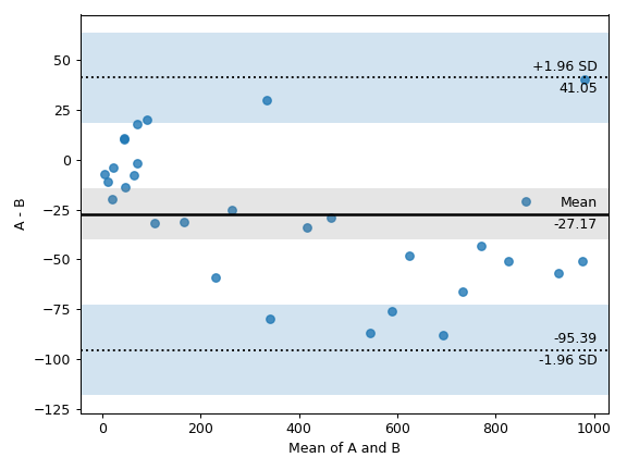
On this page
[Edit on GitHub](https://github.com/raphaelvallat/pingouin/edit/main/docs/generated/pingouin.plot_blandaltman.rst)
---
# pingouin.plot_paired — pingouin 0.5.5 documentation
[Skip to main content](https://pingouin-stats.org/build/html/generated/pingouin.plot_paired.html#main-content)
Back to top
Ctrl+K
* [GitHub](https://github.com/raphaelvallat/pingouin "GitHub")
pingouin.plot\_paired[#](https://pingouin-stats.org/build/html/generated/pingouin.plot_paired.html#pingouin-plot-paired "Link to this heading")
================================================================================================================================================
pingouin.plot\_paired(_data\=None_, _dv\=None_, _within\=None_, _subject\=None_, _order\=None_, _boxplot\=True_, _boxplot\_in\_front\=False_, _orient\='v'_, _ax\=None_, _colors\=\['green', 'grey', 'indianred'\]_, _pointplot\_kwargs\={'marker': '.', 'scale': 0.6}_, _boxplot\_kwargs\={'color': 'lightslategrey', 'width': 0.2}_)[\[source\]](https://pingouin-stats.org/build/html/_modules/pingouin/plotting.html#plot_paired)
[#](https://pingouin-stats.org/build/html/generated/pingouin.plot_paired.html#pingouin.plot_paired "Link to this definition")
Paired plot.
Parameters:
**data**[`pandas.DataFrame`](https://pandas.pydata.org/pandas-docs/stable/reference/api/pandas.DataFrame.html#pandas.DataFrame "(in pandas v2.2.2)")
Long-format dataFrame.
**dv**string
Name of column containing the dependent variable.
**within**string
Name of column containing the within-subject factor.
**subject**string
Name of column containing the subject identifier.
**order**list of str
List of values in `within` that define the order of elements on the x-axis of the plot. If None, uses alphabetical order.
**boxplot**boolean
If True, add a boxplot to the paired lines using the [`seaborn.boxplot()`](https://seaborn.pydata.org/generated/seaborn.boxplot.html#seaborn.boxplot "(in seaborn v0.13.2)")
function.
**boxplot\_in\_front**boolean
If True, the boxplot is plotted on the foreground (i.e. above the individual lines) and with a slight transparency. This makes the overall plot more readable when plotting a large numbers of subjects.
Added in version 0.3.8.
**orient**string
Plot the boxplots vertically and the subjects on the x-axis if `orient='v'` (default). Set to `orient='h'` to rotate the plot by by 90 degrees.
Added in version 0.3.9.
**ax**matplotlib axes
Axis on which to draw the plot.
**colors**list of str
Line colors names. Default is green when value increases from A to B, indianred when value decreases from A to B and grey when the value is the same in both measurements.
**pointplot\_kwargs**dict
Dictionnary of optional arguments that are passed to the [`seaborn.pointplot()`](https://seaborn.pydata.org/generated/seaborn.pointplot.html#seaborn.pointplot "(in seaborn v0.13.2)")
function.
**boxplot\_kwargs**dict
Dictionnary of optional arguments that are passed to the [`seaborn.boxplot()`](https://seaborn.pydata.org/generated/seaborn.boxplot.html#seaborn.boxplot "(in seaborn v0.13.2)")
function.
Returns:
**ax**Matplotlib Axes instance
Returns the Axes object with the plot for further tweaking.
Notes
Data must be a long-format pandas DataFrame. Missing values are automatically removed using a strict listwise approach (= complete-case analysis).
Examples
Default paired plot:
\>>> import pingouin as pg
\>>> df \= pg.read\_dataset('mixed\_anova').query("Time != 'January'")
\>>> df \= df.query("Group == 'Meditation' and Subject > 40")
\>>> ax \= pg.plot\_paired(data\=df, dv\='Scores', within\='Time', subject\='Subject')

Paired plot on an existing axis (no boxplot and uniform color):
\>>> import pingouin as pg
\>>> import matplotlib.pyplot as plt
\>>> df \= pg.read\_dataset('mixed\_anova').query("Time != 'January'")
\>>> df \= df.query("Group == 'Meditation' and Subject > 40")
\>>> fig, ax1 \= plt.subplots(1, 1, figsize\=(5, 4))
\>>> pg.plot\_paired(data\=df, dv\='Scores', within\='Time',
... subject\='Subject', ax\=ax1, boxplot\=False,
... colors\=\['grey', 'grey', 'grey'\])
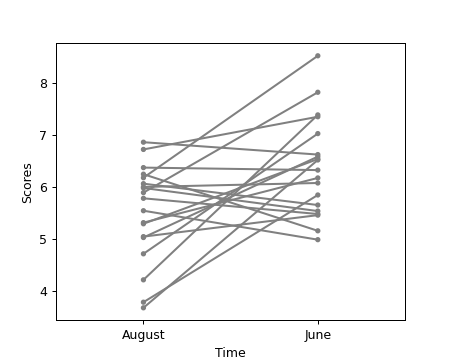
Horizontal paired plot with three unique within-levels:
\>>> import pingouin as pg
\>>> import matplotlib.pyplot as plt
\>>> df \= pg.read\_dataset('mixed\_anova').query("Group == 'Meditation'")
\>>> \# df = df.query("Group == 'Meditation' and Subject > 40")
\>>> pg.plot\_paired(data\=df, dv\='Scores', within\='Time',
... subject\='Subject', orient\='h')

With the boxplot on the foreground:
\>>> import pingouin as pg
\>>> df \= pg.read\_dataset('mixed\_anova').query("Time != 'January'")
\>>> df \= df.query("Group == 'Control'")
\>>> ax \= pg.plot\_paired(data\=df, dv\='Scores', within\='Time',
... subject\='Subject', boxplot\_in\_front\=True)
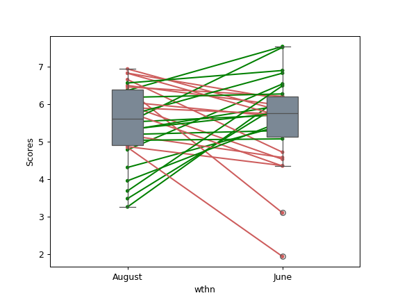
On this page
[Edit on GitHub](https://github.com/raphaelvallat/pingouin/edit/main/docs/generated/pingouin.plot_paired.rst)
---
# pingouin.plot_shift — pingouin 0.5.5 documentation
[Skip to main content](https://pingouin-stats.org/build/html/generated/pingouin.plot_shift.html#main-content)
Back to top
Ctrl+K
* [GitHub](https://github.com/raphaelvallat/pingouin "GitHub")
pingouin.plot\_shift[#](https://pingouin-stats.org/build/html/generated/pingouin.plot_shift.html#pingouin-plot-shift "Link to this heading")
=============================================================================================================================================
pingouin.plot\_shift(_x_, _y_, _paired\=False_, _n\_boot\=1000_, _percentiles\=array(\[10, 20, 30, 40, 50, 60, 70, 80, 90\])_, _confidence\=0.95_, _seed\=None_, _show\_median\=True_, _violin\=True_)[\[source\]](https://pingouin-stats.org/build/html/_modules/pingouin/plotting.html#plot_shift)
[#](https://pingouin-stats.org/build/html/generated/pingouin.plot_shift.html#pingouin.plot_shift "Link to this definition")
Shift plot.
Parameters:
**x, y**array\_like
First and second set of observations.
**paired**bool
Specify whether `x` and `y` are related (i.e. repeated measures) or independent.
Added in version 0.3.0.
**n\_boot**int
Number of bootstrap iterations. The higher, the better, the slower.
**percentiles: array\_like**
Sequence of percentiles to compute, which must be between 0 and 100 inclusive. Default set to \[10, 20, 30, 40, 50, 60, 70, 80, 90\].
**confidence**float
Confidence level (0.95 = 95%) for the confidence intervals.
**seed**int or None
Random seed for generating bootstrap samples, can be integer or None for no seed (default).
**show\_median: boolean**
If True (default), show the median with black lines.
**violin: boolean**
If True (default), plot the density of X and Y distributions. Defaut set to True.
Returns:
**fig**matplotlib Figure instance
Matplotlib Figure. To get the individual axes, use fig.axes.
See also
[`harrelldavis`](https://pingouin-stats.org/build/html/generated/pingouin.harrelldavis.html#pingouin.harrelldavis "pingouin.harrelldavis")
Notes
The shift plot is described in [\[1\]](https://pingouin-stats.org/build/html/generated/pingouin.plot_shift.html#rff4b96c9b138-1)
. It computes a shift function [\[2\]](https://pingouin-stats.org/build/html/generated/pingouin.plot_shift.html#rff4b96c9b138-2)
for two (in)dependent groups using the robust Harrell-Davis quantile estimator in conjunction with bias-corrected bootstrap confidence intervals.
References
\[[1](https://pingouin-stats.org/build/html/generated/pingouin.plot_shift.html#id1)\
\]
Rousselet, G. A., Pernet, C. R. and Wilcox, R. R. (2017). Beyond differences in means: robust graphical methods to compare two groups in neuroscience. Eur J Neurosci, 46: 1738-1748. doi:10.1111/ejn.13610
\[[2](https://pingouin-stats.org/build/html/generated/pingouin.plot_shift.html#id2)\
\]
[https://garstats.wordpress.com/2016/07/12/shift-function/](https://garstats.wordpress.com/2016/07/12/shift-function/)
Examples
Default shift plot
\>>> import numpy as np
\>>> import pingouin as pg
\>>> np.random.seed(42)
\>>> x \= np.random.normal(5.5, 2, 50)
\>>> y \= np.random.normal(6, 1.5, 50)
\>>> fig \= pg.plot\_shift(x, y)
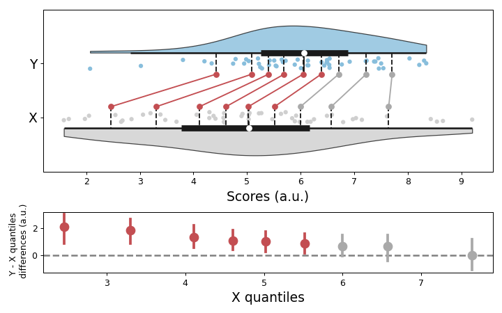
With different options, and custom axes labels
\>>> import pingouin as pg
\>>> import matplotlib.pyplot as plt
\>>> data \= pg.read\_dataset("pairwise\_corr")
\>>> fig \= pg.plot\_shift(data\["Neuroticism"\], data\["Conscientiousness"\], paired\=True,
... n\_boot\=2000, percentiles\=\[25, 50, 75\], show\_median\=False, seed\=456,
... violin\=False)
\>>> fig.axes\[0\].set\_xlabel("Groups")
\>>> fig.axes\[0\].set\_ylabel("Values", size\=15)
\>>> fig.axes\[0\].set\_title("Comparing Neuroticism and Conscientiousness", size\=15)
\>>> fig.axes\[1\].set\_xlabel("Neuroticism quantiles", size\=12)
\>>> plt.tight\_layout()
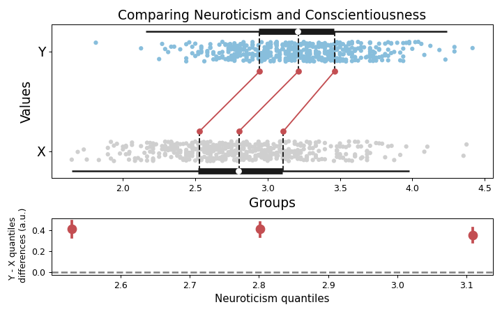
On this page
[Edit on GitHub](https://github.com/raphaelvallat/pingouin/edit/main/docs/generated/pingouin.plot_shift.rst)
---
# pingouin.plot_circmean — pingouin 0.5.5 documentation
[Skip to main content](https://pingouin-stats.org/build/html/generated/pingouin.plot_circmean.html#main-content)
Back to top
Ctrl+K
* [GitHub](https://github.com/raphaelvallat/pingouin "GitHub")
pingouin.plot\_circmean[#](https://pingouin-stats.org/build/html/generated/pingouin.plot_circmean.html#pingouin-plot-circmean "Link to this heading")
======================================================================================================================================================
pingouin.plot\_circmean(_angles_, _square\=True_, _ax\=None_, _kwargs\_markers\={'color': 'tab:blue', 'marker': 'o', 'mfc': 'none', 'ms': 10}_, _kwargs\_arrow\={'ec': 'tab:red', 'fc': 'tab:red', 'head\_length': 0.1, 'head\_width': 0.1, 'width': 0.01}_)[\[source\]](https://pingouin-stats.org/build/html/_modules/pingouin/plotting.html#plot_circmean)
[#](https://pingouin-stats.org/build/html/generated/pingouin.plot_circmean.html#pingouin.plot_circmean "Link to this definition")
Plot the circular mean and vector length of a set of angles on the unit circle.
Added in version 0.3.3.
Parameters:
**angles**array or list
Angles (expressed in radians). Only 1D array are supported here.
**square: bool**
If True (default), ensure equal aspect ratio between X and Y axes.
**ax**matplotlib axes
Axis on which to draw the plot.
**kwargs\_markers**dict
Optional keywords arguments that are passed to [`matplotlib.axes.Axes.plot`](https://matplotlib.org/stable/api/_as_gen/matplotlib.axes.Axes.plot.html#matplotlib.axes.Axes.plot "(in Matplotlib v3.9.2)")
to control the markers aesthetics.
**kwargs\_arrow**dict
Optional keywords arguments that are passed to [`matplotlib.axes.Axes.arrow`](https://matplotlib.org/stable/api/_as_gen/matplotlib.axes.Axes.arrow.html#matplotlib.axes.Axes.arrow "(in Matplotlib v3.9.2)")
to control the arrow aesthetics.
Returns:
**ax**Matplotlib Axes instance
Returns the Axes object with the plot for further tweaking.
Examples
Default plot
\>>> import pingouin as pg
\>>> ax \= pg.plot\_circmean(\[0.05, \-0.8, 1.2, 0.8, 0.5, \-0.3, 0.3, 0.7\])
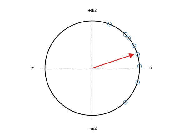
Changing some aesthetics parameters
\>>> import pingouin as pg
\>>> import matplotlib.pyplot as plt
\>>> \_, ax \= plt.subplots(1, 1, figsize\=(3, 3))
\>>> ax \= pg.plot\_circmean(\[0.05, \-0.8, 1.2, 0.8, 0.5, \-0.3, 0.3, 0.7\],
... kwargs\_markers\=dict(color\='k', mfc\='k'),
... kwargs\_arrow\=dict(ec\='k', fc\='k'), ax\=ax)
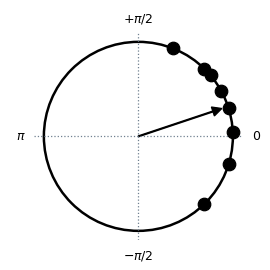
\>>> import pingouin as pg
\>>> import seaborn as sns
\>>> sns.set(font\_scale\=1.5, style\='white')
\>>> ax \= pg.plot\_circmean(\[0.8, 1.5, 3.14, 5.2, 6.1, 2.8, 2.6, 3.2\],
... kwargs\_markers\=dict(marker\="None"))
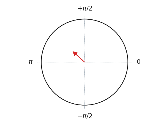
On this page
[Edit on GitHub](https://github.com/raphaelvallat/pingouin/edit/main/docs/generated/pingouin.plot_circmean.rst)
---
# pingouin.plot_rm_corr — pingouin 0.5.5 documentation
[Skip to main content](https://pingouin-stats.org/build/html/generated/pingouin.plot_rm_corr.html#main-content)
Back to top
Ctrl+K
* [GitHub](https://github.com/raphaelvallat/pingouin "GitHub")
pingouin.plot\_rm\_corr[#](https://pingouin-stats.org/build/html/generated/pingouin.plot_rm_corr.html#pingouin-plot-rm-corr "Link to this heading")
====================================================================================================================================================
pingouin.plot\_rm\_corr(_data\=None_, _x\=None_, _y\=None_, _subject\=None_, _legend\=False_, _kwargs\_facetgrid\={'aspect': 1, 'height': 4}_, _kwargs\_line\={'ls': 'solid'}_, _kwargs\_scatter\={'marker': 'o'}_)[\[source\]](https://pingouin-stats.org/build/html/_modules/pingouin/plotting.html#plot_rm_corr)
[#](https://pingouin-stats.org/build/html/generated/pingouin.plot_rm_corr.html#pingouin.plot_rm_corr "Link to this definition")
Plot a repeated measures correlation.
Parameters:
**data**[`pandas.DataFrame`](https://pandas.pydata.org/pandas-docs/stable/reference/api/pandas.DataFrame.html#pandas.DataFrame "(in pandas v2.2.2)")
Dataframe.
**x, y**string
Name of columns in `data` containing the two dependent variables.
**subject**string
Name of column in `data` containing the subject indicator.
**legend**boolean
If True, add legend to plot. Legend will show all the unique values in `subject`.
**kwargs\_facetgrid**dict
Optional keyword arguments passed to [`seaborn.FacetGrid`](https://seaborn.pydata.org/generated/seaborn.FacetGrid.html#seaborn.FacetGrid "(in seaborn v0.13.2)")
**kwargs\_line**dict
Optional keyword arguments passed to `matplotlib.pyplot.plot`
**kwargs\_scatter**dict
Optional keyword arguments passed to `matplotlib.pyplot.scatter`
Returns:
**g**[`seaborn.FacetGrid`](https://seaborn.pydata.org/generated/seaborn.FacetGrid.html#seaborn.FacetGrid "(in seaborn v0.13.2)")
Seaborn FacetGrid.
See also
[`rm_corr`](https://pingouin-stats.org/build/html/generated/pingouin.rm_corr.html#pingouin.rm_corr "pingouin.rm_corr")
Notes
Repeated measures correlation [\[1\]](https://pingouin-stats.org/build/html/generated/pingouin.plot_rm_corr.html#ra432921dd5c1-1)
(rmcorr) is a statistical technique for determining the common within-individual association for paired measures assessed on two or more occasions for multiple individuals.
Results have been tested against the rmcorr R package. Note that this function requires [statsmodels](https://www.statsmodels.org/stable/index.html)
.
Missing values are automatically removed from the `data` (listwise deletion).
References
\[[1](https://pingouin-stats.org/build/html/generated/pingouin.plot_rm_corr.html#id1)\
\]
Bakdash, J.Z., Marusich, L.R., 2017. Repeated Measures Correlation. Front. Psychol. 8, 456. [https://doi.org/10.3389/fpsyg.2017.00456](https://doi.org/10.3389/fpsyg.2017.00456)
Examples
Default repeated mesures correlation plot
\>>> import pingouin as pg
\>>> df \= pg.read\_dataset('rm\_corr')
\>>> g \= pg.plot\_rm\_corr(data\=df, x\='pH', y\='PacO2', subject\='Subject')
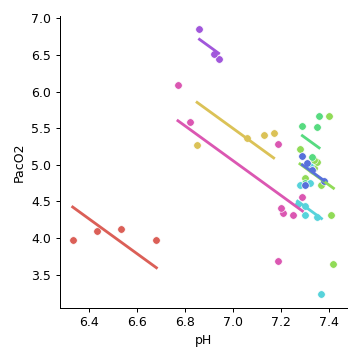
With some tweakings
\>>> import pingouin as pg
\>>> import seaborn as sns
\>>> df \= pg.read\_dataset('rm\_corr')
\>>> sns.set(style\='darkgrid', font\_scale\=1.2)
\>>> g \= pg.plot\_rm\_corr(data\=df, x\='pH', y\='PacO2',
... subject\='Subject', legend\=True,
... kwargs\_facetgrid\=dict(height\=4.5, aspect\=1.5,
... palette\='Spectral'))
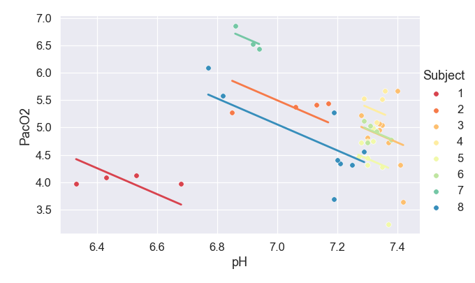
On this page
[Edit on GitHub](https://github.com/raphaelvallat/pingouin/edit/main/docs/generated/pingouin.plot_rm_corr.rst)
---
# pingouin.power_chi2 — pingouin 0.5.5 documentation
[Skip to main content](https://pingouin-stats.org/build/html/generated/pingouin.power_chi2.html#main-content)
Back to top
Ctrl+K
* [GitHub](https://github.com/raphaelvallat/pingouin "GitHub")
pingouin.power\_chi2[#](https://pingouin-stats.org/build/html/generated/pingouin.power_chi2.html#pingouin-power-chi2 "Link to this heading")
=============================================================================================================================================
pingouin.power\_chi2(_dof_, _w\=None_, _n\=None_, _power\=None_, _alpha\=0.05_)[\[source\]](https://pingouin-stats.org/build/html/_modules/pingouin/power.html#power_chi2)
[#](https://pingouin-stats.org/build/html/generated/pingouin.power_chi2.html#pingouin.power_chi2 "Link to this definition")
Evaluate power, sample size, effect size or significance level of chi-squared tests.
Parameters:
**dof**float
Degree of freedom (depends on the chosen test).
**w**float
Cohen’s w effect size [\[1\]](https://pingouin-stats.org/build/html/generated/pingouin.power_chi2.html#rbd2aa07349f2-1)
.
**n**int
Total number of observations.
**power**float
Test power (= 1 - type II error).
**alpha**float
Significance level (type I error probability). The default is 0.05.
Notes
Exactly ONE of the parameters `w`, `n`, `power` and `alpha` must be passed as None, and that parameter is determined from the others. The degrees of freedom `dof` must always be specified.
`alpha` has a default value of 0.05 so None must be explicitly passed if you want to compute it.
This function is a Python adaptation of the pwr.chisq.test function implemented in the [pwr](https://cran.r-project.org/web/packages/pwr/pwr.pdf)
R package.
Statistical power is the likelihood that a study will detect an effect when there is an effect there to be detected. A high statistical power means that there is a low probability of concluding that there is no effect when there is one. Statistical power is mainly affected by the effect size and the sample size.
The non-centrality parameter is defined by:
\\\[\\delta = N \* w^2\\\]
Then the critical value is computed using the percentile point function of the \\(\\chi^2\\) distribution with the alpha level and degrees of freedom.
Finally, the power of the chi-squared test is calculated using the survival function of the non-central \\(\\chi^2\\) distribution using the previously computed critical value, non-centrality parameter, and the degrees of freedom of the test.
[`scipy.optimize.brenth()`](https://docs.scipy.org/doc/scipy/reference/generated/scipy.optimize.brenth.html#scipy.optimize.brenth "(in SciPy v1.14.1)")
is used to solve power equations for other variables (i.e. sample size, effect size, or significance level). If the solving fails, a nan value is returned.
Results have been tested against GPower and the [pwr](https://cran.r-project.org/web/packages/pwr/pwr.pdf)
R package.
References
\[[1](https://pingouin-stats.org/build/html/generated/pingouin.power_chi2.html#id1)\
\]
Cohen, J. (1988). Statistical power analysis for the behavioral sciences (2nd ed.).
Examples
1. Compute achieved power
\>>> from pingouin import power\_chi2
\>>> print('power: %.4f' % power\_chi2(dof\=1, w\=0.3, n\=20))
power: 0.2687
2. Compute required sample size
\>>> print('n: %.4f' % power\_chi2(dof\=3, w\=0.3, power\=0.80))
n: 121.1396
3. Compute achieved effect size
\>>> print('w: %.4f' % power\_chi2(dof\=2, n\=20, power\=0.80, alpha\=0.05))
w: 0.6941
4. Compute achieved alpha (significance)
\>>> print('alpha: %.4f' % power\_chi2(dof\=1, w\=0.5, n\=20, power\=0.80, alpha\=None))
alpha: 0.1630
On this page
[Edit on GitHub](https://github.com/raphaelvallat/pingouin/edit/main/docs/generated/pingouin.power_chi2.rst)
---
# pingouin.power_corr — pingouin 0.5.5 documentation
[Skip to main content](https://pingouin-stats.org/build/html/generated/pingouin.power_corr.html#main-content)
Back to top
Ctrl+K
* [GitHub](https://github.com/raphaelvallat/pingouin "GitHub")
pingouin.power\_corr[#](https://pingouin-stats.org/build/html/generated/pingouin.power_corr.html#pingouin-power-corr "Link to this heading")
=============================================================================================================================================
pingouin.power\_corr(_r\=None_, _n\=None_, _power\=None_, _alpha\=0.05_, _alternative\='two-sided'_)[\[source\]](https://pingouin-stats.org/build/html/_modules/pingouin/power.html#power_corr)
[#](https://pingouin-stats.org/build/html/generated/pingouin.power_corr.html#pingouin.power_corr "Link to this definition")
Evaluate power, sample size, correlation coefficient or significance level of a correlation test.
Parameters:
**r**float
Correlation coefficient.
**n**int
Number of observations (sample size).
**power**float
Test power (= 1 - type II error).
**alpha**float
Significance level (type I error probability). The default is 0.05.
**alternative**string
Defines the alternative hypothesis, or tail of the correlation. Must be one of “two-sided” (default), “greater” or “less”. Both “greater” and “less” return a one-sided p-value. “greater” tests against the alternative hypothesis that the correlation is positive (greater than zero), “less” tests against the hypothesis that the correlation is negative.
Notes
Exactly ONE of the parameters `r`, `n`, `power` and `alpha` must be passed as None, and that parameter is determined from the others.
`alpha` has a default value of 0.05 so None must be explicitly passed if you want to compute it.
[`scipy.optimize.brenth()`](https://docs.scipy.org/doc/scipy/reference/generated/scipy.optimize.brenth.html#scipy.optimize.brenth "(in SciPy v1.14.1)")
is used to solve power equations for other variables (i.e. sample size, effect size, or significance level). If the solving fails, a nan value is returned.
This function is a Python adaptation of the pwr.r.test function implemented in the [pwr](https://cran.r-project.org/web/packages/pwr/pwr.pdf)
R package.
Examples
1. Compute achieved power given `r`, `n` and `alpha`
\>>> from pingouin import power\_corr
\>>> print('power: %.4f' % power\_corr(r\=0.5, n\=20))
power: 0.6379
2. Same but one-sided test
\>>> print('power: %.4f' % power\_corr(r\=0.5, n\=20, alternative\="greater"))
power: 0.7510
\>>> print('power: %.4f' % power\_corr(r\=0.5, n\=20, alternative\="less"))
power: 0.0000
3. Compute required sample size given `r`, `power` and `alpha`
\>>> print('n: %.4f' % power\_corr(r\=0.5, power\=0.80))
n: 28.2484
4. Compute achieved `r` given `n`, `power` and `alpha` level
\>>> print('r: %.4f' % power\_corr(n\=20, power\=0.80, alpha\=0.05))
r: 0.5822
5. Compute achieved alpha level given `r`, `n` and `power`
\>>> print('alpha: %.4f' % power\_corr(r\=0.5, n\=20, power\=0.80, alpha\=None))
alpha: 0.1377
On this page
[Edit on GitHub](https://github.com/raphaelvallat/pingouin/edit/main/docs/generated/pingouin.power_corr.rst)
---
# pingouin.power_anova — pingouin 0.5.5 documentation
[Skip to main content](https://pingouin-stats.org/build/html/generated/pingouin.power_anova.html#main-content)
Back to top
Ctrl+K
* [GitHub](https://github.com/raphaelvallat/pingouin "GitHub")
pingouin.power\_anova[#](https://pingouin-stats.org/build/html/generated/pingouin.power_anova.html#pingouin-power-anova "Link to this heading")
================================================================================================================================================
pingouin.power\_anova(_eta\_squared\=None_, _k\=None_, _n\=None_, _power\=None_, _alpha\=0.05_)[\[source\]](https://pingouin-stats.org/build/html/_modules/pingouin/power.html#power_anova)
[#](https://pingouin-stats.org/build/html/generated/pingouin.power_anova.html#pingouin.power_anova "Link to this definition")
Evaluate power, sample size, effect size or significance level of a one-way balanced ANOVA.
Parameters:
**eta\_squared**float
ANOVA effect size (eta-squared, \\(\\eta^2\\)).
**k**int
Number of groups
**n**int
Sample size per group. Groups are assumed to be balanced (i.e. same sample size).
**power**float
Test power (= 1 - type II error).
**alpha**float
Significance level \\(\\alpha\\) (type I error probability). The default is 0.05.
Notes
Exactly ONE of the parameters `eta_squared`, `k`, `n`, `power` and `alpha` must be passed as None, and that parameter is determined from the others.
`alpha` has a default value of 0.05 so None must be explicitly passed if you want to compute it.
This function is a Python adaptation of the pwr.anova.test function implemented in the [pwr](https://cran.r-project.org/web/packages/pwr/pwr.pdf)
R package.
Statistical power is the likelihood that a study will detect an effect when there is an effect there to be detected. A high statistical power means that there is a low probability of concluding that there is no effect when there is one. Statistical power is mainly affected by the effect size and the sample size.
For one-way ANOVA, eta-squared is the same as partial eta-squared. It can be evaluated from the F-value (\\(F^\*\\)) and the degrees of freedom of the ANOVA (\\(v\_1, v\_2\\)) using the following formula:
\\\[\\eta^2 = \\frac{v\_1 F^\*}{v\_1 F^\* + v\_2}\\\]
GPower uses the \\(f\\) effect size instead of the \\(\\eta^2\\). The formula to convert from one to the other are given below:
\\\[f = \\sqrt{\\frac{\\eta^2}{1 - \\eta^2}}\\\]
\\\[\\eta^2 = \\frac{f^2}{1 + f^2}\\\]
Using \\(\\eta^2\\) and the total sample size \\(N\\), the non-centrality parameter is defined by:
\\\[\\delta = N \* \\frac{\\eta^2}{1 - \\eta^2}\\\]
Then the critical value of the non-central F-distribution is computed using the percentile point function of the F-distribution with:
\\\[q = 1 - \\alpha\\\]
\\\[v\_1 = k - 1\\\]
\\\[v\_2 = N - k\\\]
where \\(k\\) is the number of groups.
Finally, the power of the ANOVA is calculated using the survival function of the non-central F-distribution using the previously computed critical value, non-centrality parameter, and degrees of freedom.
[`scipy.optimize.brenth()`](https://docs.scipy.org/doc/scipy/reference/generated/scipy.optimize.brenth.html#scipy.optimize.brenth "(in SciPy v1.14.1)")
is used to solve power equations for other variables (i.e. sample size, effect size, or significance level). If the solving fails, a nan value is returned.
Results have been tested against GPower and the [pwr](https://cran.r-project.org/web/packages/pwr/pwr.pdf)
R package.
Examples
1. Compute achieved power
\>>> from pingouin import power\_anova
\>>> print('power: %.4f' % power\_anova(eta\_squared\=0.1, k\=3, n\=20))
power: 0.6082
2. Compute required number of groups
\>>> print('k: %.4f' % power\_anova(eta\_squared\=0.1, n\=20, power\=0.80))
k: 6.0944
3. Compute required sample size
\>>> print('n: %.4f' % power\_anova(eta\_squared\=0.1, k\=3, power\=0.80))
n: 29.9256
4. Compute achieved effect size
\>>> print('eta-squared: %.4f' % power\_anova(n\=20, k\=4, power\=0.80, alpha\=0.05))
eta-squared: 0.1255
5. Compute achieved alpha (significance)
\>>> print('alpha: %.4f' % power\_anova(eta\_squared\=0.1, n\=20, k\=4, power\=0.80, alpha\=None))
alpha: 0.1085
On this page
[Edit on GitHub](https://github.com/raphaelvallat/pingouin/edit/main/docs/generated/pingouin.power_anova.rst)
---
# pingouin.power_rm_anova — pingouin 0.5.5 documentation
[Skip to main content](https://pingouin-stats.org/build/html/generated/pingouin.power_rm_anova.html#main-content)
Back to top
Ctrl+K
* [GitHub](https://github.com/raphaelvallat/pingouin "GitHub")
pingouin.power\_rm\_anova[#](https://pingouin-stats.org/build/html/generated/pingouin.power_rm_anova.html#pingouin-power-rm-anova "Link to this heading")
==========================================================================================================================================================
pingouin.power\_rm\_anova(_eta\_squared\=None_, _m\=None_, _n\=None_, _power\=None_, _alpha\=0.05_, _corr\=0.5_, _epsilon\=1_)[\[source\]](https://pingouin-stats.org/build/html/_modules/pingouin/power.html#power_rm_anova)
[#](https://pingouin-stats.org/build/html/generated/pingouin.power_rm_anova.html#pingouin.power_rm_anova "Link to this definition")
Evaluate power, sample size, effect size or significance level of a balanced one-way repeated measures ANOVA.
Parameters:
**eta\_squared**float
ANOVA effect size (eta-squared, \\(\\eta^2\\)).
**m**int
Number of repeated measurements.
**n**int
Sample size per measurement. All measurements must have the same sample size.
**power**float
Test power (= 1 - type II error).
**alpha**float
Significance level \\(\\alpha\\) (type I error probability). The default is 0.05.
**corr**float
Average correlation coefficient among repeated measurements. The default is \\(r=0.5\\).
**epsilon**float
Epsilon adjustement factor for sphericity. This can be calculated using the [`pingouin.epsilon()`](https://pingouin-stats.org/build/html/generated/pingouin.epsilon.html#pingouin.epsilon "pingouin.epsilon")
function.
Notes
Exactly ONE of the parameters `eta_squared`, `m`, `n`, `power` and `alpha` must be passed as None, and that parameter is determined from the others.
`alpha` has a default value of 0.05 so None must be explicitly passed if you want to compute it.
Statistical power is the likelihood that a study will detect an effect when there is an effect there to be detected. A high statistical power means that there is a low probability of concluding that there is no effect when there is one. Statistical power is mainly affected by the effect size and the sample size.
GPower uses the \\(f\\) effect size instead of the \\(\\eta^2\\). The formula to convert from one to the other are given below:
\\\[f = \\sqrt{\\frac{\\eta^2}{1 - \\eta^2}}\\\]
\\\[\\eta^2 = \\frac{f^2}{1 + f^2}\\\]
Using \\(\\eta^2\\), the sample size \\(N\\), the number of repeated measurements \\(m\\), the epsilon correction factor \\(\\epsilon\\) (see [`pingouin.epsilon()`](https://pingouin-stats.org/build/html/generated/pingouin.epsilon.html#pingouin.epsilon "pingouin.epsilon")
), and the average correlation between the repeated measures \\(c\\), one can then calculate the non-centrality parameter as follow:
\\\[\\delta = \\frac{f^2 \* N \* m \* \\epsilon}{1 - c}\\\]
Then the critical value of the non-central F-distribution is computed using the percentile point function of the F-distribution with:
\\\[q = 1 - \\alpha\\\]
\\\[v\_1 = (m - 1) \* \\epsilon\\\]
\\\[v\_2 = (N - 1) \* v\_1\\\]
Finally, the power of the ANOVA is calculated using the survival function of the non-central F-distribution using the previously computed critical value, non-centrality parameter, and degrees of freedom.
[`scipy.optimize.brenth()`](https://docs.scipy.org/doc/scipy/reference/generated/scipy.optimize.brenth.html#scipy.optimize.brenth "(in SciPy v1.14.1)")
is used to solve power equations for other variables (i.e. sample size, effect size, or significance level). If the solving fails, a nan value is returned.
Results have been tested against GPower and the [pwr](https://cran.r-project.org/web/packages/pwr/pwr.pdf)
R package.
Examples
1. Compute achieved power
\>>> from pingouin import power\_rm\_anova
\>>> print('power: %.4f' % power\_rm\_anova(eta\_squared\=0.1, m\=3, n\=20))
power: 0.8913
2. Compute required number of groups
\>>> print('m: %.4f' % power\_rm\_anova(eta\_squared\=0.1, n\=20, power\=0.90))
m: 3.1347
3. Compute required sample size
\>>> print('n: %.4f' % power\_rm\_anova(eta\_squared\=0.1, m\=3, power\=0.80))
n: 15.9979
4. Compute achieved effect size
\>>> print('eta-squared: %.4f' % power\_rm\_anova(n\=20, m\=4, power\=0.80, alpha\=0.05))
eta-squared: 0.0680
5. Compute achieved alpha (significance)
\>>> print('alpha: %.4f' % power\_rm\_anova(eta\_squared\=0.1, n\=20, m\=4, power\=0.80, alpha\=None))
alpha: 0.0081
Let’s take a more concrete example. First, we’ll load a repeated measures dataset in wide-format. Each row is an observation (e.g. a subject), and each column a successive repeated measurements (e.g t=0, t=1, …).
\>>> import pingouin as pg
\>>> data \= pg.read\_dataset('rm\_anova\_wide')
\>>> data.head()
Before 1 week 2 week 3 week
0 4.3 5.3 4.8 6.3
1 3.9 2.3 5.6 4.3
2 4.5 2.6 4.1 NaN
3 5.1 4.2 6.0 6.3
4 3.8 3.6 4.8 6.8
Note that this dataset has some missing values. We’ll simply delete any row with one or more missing values, and then compute a repeated measures ANOVA:
\>>> data \= data.dropna()
\>>> pg.rm\_anova(data, effsize\="n2").round(3)
Source ddof1 ddof2 F p-unc n2 eps
0 Within 3 24 5.201 0.007 0.346 0.694
The repeated measures ANOVA is significant at the 0.05 level. Now, we can easily compute the power of the ANOVA with the information in the ANOVA table:
\>>> \# n is the sample size and m is the number of repeated measures
\>>> n, m \= data.shape
\>>> round(pg.power\_rm\_anova(eta\_squared\=0.346, m\=m, n\=n, epsilon\=0.694), 3)
0.99
Our ANOVA has a very high statistical power. However, to be even more accurate in our power calculation, we should also fill in the average correlation among repeated measurements. Since our dataframe is in wide-format (with each column being a successive measurement), this can be done by taking the mean of the superdiagonal of the correlation matrix, which is similar to manually calculating the correlation between each successive pairwise measurements and then taking the mean. Since correlation coefficients are not normally distributed, we use the _r-to-z_ transform prior to averaging (`numpy.arctanh()`), and then the _z-to-r_ transform (`numpy.tanh()`) to convert back to a correlation coefficient. This gives a more precise estimate of the mean.
\>>> import numpy as np
\>>> corr \= np.diag(data.corr(), k\=1)
\>>> avgcorr \= np.tanh(np.arctanh(corr).mean())
\>>> round(avgcorr, 4)
\-0.1996
In this example, we’re using a fake dataset and the average correlation is negative. However, it will most likely be positive with real data. Let’s now compute the final power of the repeated measures ANOVA:
\>>> round(pg.power\_rm\_anova(eta\_squared\=0.346, m\=m, n\=n, epsilon\=0.694, corr\=avgcorr), 3)
0.771
On this page
[Edit on GitHub](https://github.com/raphaelvallat/pingouin/edit/main/docs/generated/pingouin.power_rm_anova.rst)
---
# pingouin.power_ttest2n — pingouin 0.5.5 documentation
[Skip to main content](https://pingouin-stats.org/build/html/generated/pingouin.power_ttest2n.html#main-content)
Back to top
Ctrl+K
* [GitHub](https://github.com/raphaelvallat/pingouin "GitHub")
pingouin.power\_ttest2n[#](https://pingouin-stats.org/build/html/generated/pingouin.power_ttest2n.html#pingouin-power-ttest2n "Link to this heading")
======================================================================================================================================================
pingouin.power\_ttest2n(_nx_, _ny_, _d\=None_, _power\=None_, _alpha\=0.05_, _alternative\='two-sided'_)[\[source\]](https://pingouin-stats.org/build/html/_modules/pingouin/power.html#power_ttest2n)
[#](https://pingouin-stats.org/build/html/generated/pingouin.power_ttest2n.html#pingouin.power_ttest2n "Link to this definition")
Evaluate power, effect size or significance level of an independent two-samples T-test with unequal sample sizes.
Parameters:
**nx, ny**int
Sample sizes. Must be specified. If the sample sizes are equal, you should use the [`power_ttest()`](https://pingouin-stats.org/build/html/generated/pingouin.power_ttest.html#pingouin.power_ttest "pingouin.power_ttest")
function instead.
**d**float
Cohen d effect size
**power**float
Test power (= 1 - type II error).
**alpha**float
Significance level (type I error probability). The default is 0.05.
**alternative**string
Defines the alternative hypothesis, or tail of the test. Must be one of “two-sided” (default), “greater” or “less”.
Notes
Exactly ONE of the parameters `d`, `power` and `alpha` must be passed as None, and that parameter is determined from the others.
`alpha` has a default value of 0.05 so None must be explicitly passed if you want to compute it.
This function is a Python adaptation of the pwr.t2n.test function implemented in the [pwr](https://cran.r-project.org/web/packages/pwr/pwr.pdf)
R package.
Statistical power is the likelihood that a study will detect an effect when there is an effect there to be detected. A high statistical power means that there is a low probability of concluding that there is no effect when there is one. Statistical power is mainly affected by the effect size and the sample size.
The first step is to use the Cohen’s d to calculate the non-centrality parameter \\(\\delta\\) and degrees of freedom \\(v\\).cIn case of two independent groups with unequal sample sizes, this is:
\\\[\\delta = d \* \\sqrt{\\frac{n\_i \* n\_j}{n\_i + n\_j}}\\\]
\\\[v = n\_i + n\_j - 2\\\]
where \\(d\\) is the Cohen d, \\(n\\) the sample size, \\(n\_i\\) the sample size of the first group and \\(n\_j\\) the sample size of the second group,
The critical value is then found using the percent point function of the T distribution with \\(q = 1 - alpha\\) and \\(v\\) degrees of freedom.
Finally, the power of the test is given by the survival function of the non-central distribution using the previously calculated critical value, degrees of freedom and non-centrality parameter.
[`scipy.optimize.brenth()`](https://docs.scipy.org/doc/scipy/reference/generated/scipy.optimize.brenth.html#scipy.optimize.brenth "(in SciPy v1.14.1)")
is used to solve power equations for other variables (i.e. sample size, effect size, or significance level). If the solving fails, a nan value is returned.
Results have been tested against GPower and the [pwr](https://cran.r-project.org/web/packages/pwr/pwr.pdf)
R package.
Examples
1. Compute achieved power of a T-test given `d`, `n` and `alpha`
\>>> from pingouin import power\_ttest2n
\>>> print('power: %.4f' % power\_ttest2n(nx\=20, ny\=15, d\=0.5, alternative\='greater'))
power: 0.4164
2. Compute achieved `d` given `n`, `power` and `alpha` level
\>>> print('d: %.4f' % power\_ttest2n(nx\=20, ny\=15, power\=0.80, alpha\=0.05))
d: 0.9859
3. Compute achieved alpha level given `d`, `n` and `power`
\>>> print('alpha: %.4f' % power\_ttest2n(nx\=20, ny\=15, d\=0.5, power\=0.80, alpha\=None))
alpha: 0.5000
On this page
[Edit on GitHub](https://github.com/raphaelvallat/pingouin/edit/main/docs/generated/pingouin.power_ttest2n.rst)
---
# pingouin.power_ttest — pingouin 0.5.5 documentation
[Skip to main content](https://pingouin-stats.org/build/html/generated/pingouin.power_ttest.html#main-content)
Back to top
Ctrl+K
* [GitHub](https://github.com/raphaelvallat/pingouin "GitHub")
pingouin.power\_ttest[#](https://pingouin-stats.org/build/html/generated/pingouin.power_ttest.html#pingouin-power-ttest "Link to this heading")
================================================================================================================================================
pingouin.power\_ttest(_d\=None_, _n\=None_, _power\=None_, _alpha\=0.05_, _contrast\='two-samples'_, _alternative\='two-sided'_)[\[source\]](https://pingouin-stats.org/build/html/_modules/pingouin/power.html#power_ttest)
[#](https://pingouin-stats.org/build/html/generated/pingouin.power_ttest.html#pingouin.power_ttest "Link to this definition")
Evaluate power, sample size, effect size or significance level of a one-sample T-test, a paired T-test or an independent two-samples T-test with equal sample sizes.
Parameters:
**d**float
Cohen d effect size
**n**int
Sample size In case of a two-sample T-test, sample sizes are assumed to be equal. Otherwise, see the [`power_ttest2n()`](https://pingouin-stats.org/build/html/generated/pingouin.power_ttest2n.html#pingouin.power_ttest2n "pingouin.power_ttest2n")
function.
**power**float
Test power (= 1 - type II error).
**alpha**float
Significance level (type I error probability). The default is 0.05.
**contrast**str
Can be “one-sample”, “two-samples” or “paired”. Note that “one-sample” and “paired” have the same behavior.
**alternative**string
Defines the alternative hypothesis, or tail of the test. Must be one of “two-sided” (default), “greater” or “less”.
Notes
Exactly ONE of the parameters `d`, `n`, `power` and `alpha` must be passed as None, and that parameter is determined from the others.
For a paired T-test, the sample size `n` corresponds to the number of pairs. For an independent two-sample T-test with equal sample sizes, `n` corresponds to the sample size of each group (i.e. number of observations in one group). If the sample sizes are unequal, please use the [`power_ttest2n()`](https://pingouin-stats.org/build/html/generated/pingouin.power_ttest2n.html#pingouin.power_ttest2n "pingouin.power_ttest2n")
function instead.
`alpha` has a default value of 0.05 so None must be explicitly passed if you want to compute it.
This function is a Python adaptation of the pwr.t.test function implemented in the [pwr](https://cran.r-project.org/web/packages/pwr/pwr.pdf)
R package.
Statistical power is the likelihood that a study will detect an effect when there is an effect there to be detected. A high statistical power means that there is a low probability of concluding that there is no effect when there is one. Statistical power is mainly affected by the effect size and the sample size.
The first step is to use the Cohen’s d to calculate the non-centrality parameter \\(\\delta\\) and degrees of freedom \\(v\\). In case of paired groups, this is:
\\\[\\delta = d \* \\sqrt n\\\]
\\\[v = n - 1\\\]
and in case of independent groups with equal sample sizes:
\\\[\\delta = d \* \\sqrt{\\frac{n}{2}}\\\]
\\\[v = (n - 1) \* 2\\\]
where \\(d\\) is the Cohen d and \\(n\\) the sample size.
The critical value is then found using the percent point function of the T distribution with \\(q = 1 - alpha\\) and \\(v\\) degrees of freedom.
Finally, the power of the test is given by the survival function of the non-central distribution using the previously calculated critical value, degrees of freedom and non-centrality parameter.
[`scipy.optimize.brenth()`](https://docs.scipy.org/doc/scipy/reference/generated/scipy.optimize.brenth.html#scipy.optimize.brenth "(in SciPy v1.14.1)")
is used to solve power equations for other variables (i.e. sample size, effect size, or significance level). If the solving fails, a nan value is returned.
Results have been tested against GPower and the [pwr](https://cran.r-project.org/web/packages/pwr/pwr.pdf)
R package.
Examples
1. Compute power of a one-sample T-test given `d`, `n` and `alpha`
\>>> from pingouin import power\_ttest
\>>> print('power: %.4f' % power\_ttest(d\=0.5, n\=20, contrast\='one-sample'))
power: 0.5645
2. Compute required sample size given `d`, `power` and `alpha`
\>>> print('n: %.4f' % power\_ttest(d\=0.5, power\=0.80, alternative\='greater'))
n: 50.1508
3. Compute achieved `d` given `n`, `power` and `alpha` level
\>>> print('d: %.4f' % power\_ttest(n\=20, power\=0.80, alpha\=0.05, contrast\='paired'))
d: 0.6604
4. Compute achieved alpha level given `d`, `n` and `power`
\>>> print('alpha: %.4f' % power\_ttest(d\=0.5, n\=20, power\=0.80, alpha\=None))
alpha: 0.4430
5. One-sided tests
\>>> from pingouin import power\_ttest
\>>> print('power: %.4f' % power\_ttest(d\=0.5, n\=20, alternative\='greater'))
power: 0.4634
\>>> print('power: %.4f' % power\_ttest(d\=0.5, n\=20, alternative\='less'))
power: 0.0007
On this page
[Edit on GitHub](https://github.com/raphaelvallat/pingouin/edit/main/docs/generated/pingouin.power_ttest.rst)
---
# pingouin.cronbach_alpha — pingouin 0.5.5 documentation
[Skip to main content](https://pingouin-stats.org/build/html/generated/pingouin.cronbach_alpha.html#main-content)
Back to top
Ctrl+K
* [GitHub](https://github.com/raphaelvallat/pingouin "GitHub")
pingouin.cronbach\_alpha[#](https://pingouin-stats.org/build/html/generated/pingouin.cronbach_alpha.html#pingouin-cronbach-alpha "Link to this heading")
=========================================================================================================================================================
pingouin.cronbach\_alpha(_data\=None_, _items\=None_, _scores\=None_, _subject\=None_, _nan\_policy\='pairwise'_, _ci\=0.95_)[\[source\]](https://pingouin-stats.org/build/html/_modules/pingouin/reliability.html#cronbach_alpha)
[#](https://pingouin-stats.org/build/html/generated/pingouin.cronbach_alpha.html#pingouin.cronbach_alpha "Link to this definition")
Cronbach’s alpha reliability measure.
Parameters:
**data**[`pandas.DataFrame`](https://pandas.pydata.org/pandas-docs/stable/reference/api/pandas.DataFrame.html#pandas.DataFrame "(in pandas v2.2.2)")
Wide or long-format dataframe.
**items**str
Column in `data` with the items names (long-format only).
**scores**str
Column in `data` with the scores (long-format only).
**subject**str
Column in `data` with the subject identifier (long-format only).
**nan\_policy**bool
If ‘listwise’, remove the entire rows that contain missing values (= listwise deletion). If ‘pairwise’ (default), only pairwise missing values are removed when computing the covariance matrix. For more details, please refer to the [`pandas.DataFrame.cov()`](https://pandas.pydata.org/pandas-docs/stable/reference/api/pandas.DataFrame.cov.html#pandas.DataFrame.cov "(in pandas v2.2.2)")
method.
**ci**float
Confidence interval (.95 = 95%)
Returns:
**alpha**float
Cronbach’s alpha
Notes
This function works with both wide and long format dataframe. If you pass a long-format dataframe, you must also pass the `items`, `scores` and `subj` columns (in which case the data will be converted into wide format using the [`pandas.DataFrame.pivot()`](https://pandas.pydata.org/pandas-docs/stable/reference/api/pandas.DataFrame.pivot.html#pandas.DataFrame.pivot "(in pandas v2.2.2)")
method).
Internal consistency is usually measured with Cronbach’s alpha [\[1\]](https://pingouin-stats.org/build/html/generated/pingouin.cronbach_alpha.html#r65a37577502b-1)
, a statistic calculated from the pairwise correlations between items. Internal consistency ranges between negative infinity and one. Coefficient alpha will be negative whenever there is greater within-subject variability than between-subject variability.
Cronbach’s \\(\\alpha\\) is defined as
\\\[\\alpha ={k \\over k-1}\\left(1-{\\sum\_{{i=1}}^{k}\\sigma\_{{y\_{i}}}^{2} \\over\\sigma\_{x}^{2}}\\right)\\\]
where \\(k\\) refers to the number of items, \\(\\sigma\_{x}^{2}\\) is the variance of the observed total scores, and \\(\\sigma\_{{y\_{i}}}^{2}\\) the variance of component \\(i\\) for the current sample of subjects.
Another formula for Cronbach’s \\(\\alpha\\) is
\\\[\\alpha = \\frac{k \\times \\bar c}{\\bar v + (k - 1) \\times \\bar c}\\\]
where \\(\\bar c\\) refers to the average of all covariances between items and \\(\\bar v\\) to the average variance of each item.
95% confidence intervals are calculated using Feldt’s method [\[2\]](https://pingouin-stats.org/build/html/generated/pingouin.cronbach_alpha.html#r65a37577502b-2)
:
\\\[ \\begin{align}\\begin{aligned}c\_L = 1 - (1 - \\alpha) \\cdot F\_{(0.025, n-1, (n-1)(k-1))}\\\\c\_U = 1 - (1 - \\alpha) \\cdot F\_{(0.975, n-1, (n-1)(k-1))}\\end{aligned}\\end{align} \\\]
where \\(n\\) is the number of subjects and \\(k\\) the number of items.
Results have been tested against the [psych](https://cran.r-project.org/web/packages/psych/psych.pdf)
R package.
References
\[[1](https://pingouin-stats.org/build/html/generated/pingouin.cronbach_alpha.html#id1)\
\]
[http://www.real-statistics.com/reliability/cronbachs-alpha/](http://www.real-statistics.com/reliability/cronbachs-alpha/)
\[[2](https://pingouin-stats.org/build/html/generated/pingouin.cronbach_alpha.html#id2)\
\]
Feldt, Leonard S., Woodruff, David J., & Salih, Fathi A. (1987). Statistical inference for coefficient alpha. Applied Psychological Measurement, 11(1):93-103.
Examples
Binary wide-format dataframe (with missing values)
\>>> import pingouin as pg
\>>> data \= pg.read\_dataset('cronbach\_wide\_missing')
\>>> \# In R: psych:alpha(data, use="pairwise")
\>>> pg.cronbach\_alpha(data\=data)
(0.732660835214447, array(\[0.435, 0.909\]))
After listwise deletion of missing values (remove the entire rows)
\>>> \# In R: psych:alpha(data, use="complete.obs")
\>>> pg.cronbach\_alpha(data\=data, nan\_policy\='listwise')
(0.8016949152542373, array(\[0.581, 0.933\]))
After imputing the missing values with the median of each column
\>>> pg.cronbach\_alpha(data\=data.fillna(data.median()))
(0.7380191693290734, array(\[0.447, 0.911\]))
Likert-type long-format dataframe
\>>> data \= pg.read\_dataset('cronbach\_alpha')
\>>> pg.cronbach\_alpha(data\=data, items\='Items', scores\='Scores',
... subject\='Subj')
(0.5917188485995826, array(\[0.195, 0.84 \]))
On this page
[Edit on GitHub](https://github.com/raphaelvallat/pingouin/edit/main/docs/generated/pingouin.cronbach_alpha.rst)
---
# pingouin.qqplot — pingouin 0.5.5 documentation
[Skip to main content](https://pingouin-stats.org/build/html/generated/pingouin.qqplot.html#main-content)
Back to top
Ctrl+K
* [GitHub](https://github.com/raphaelvallat/pingouin "GitHub")
pingouin.qqplot[#](https://pingouin-stats.org/build/html/generated/pingouin.qqplot.html#pingouin-qqplot "Link to this heading")
================================================================================================================================
pingouin.qqplot(_x_, _dist\='norm'_, _sparams\=()_, _confidence\=0.95_, _square\=True_, _ax\=None_, _\*\*kwargs_)[\[source\]](https://pingouin-stats.org/build/html/_modules/pingouin/plotting.html#qqplot)
[#](https://pingouin-stats.org/build/html/generated/pingouin.qqplot.html#pingouin.qqplot "Link to this definition")
Quantile-Quantile plot.
Parameters:
**x**array\_like
Sample data.
**dist**str or stats.distributions instance, optional
Distribution or distribution function name. The default is ‘norm’ for a normal probability plot.
**sparams**tuple, optional
Distribution-specific shape parameters (shape parameters, location, and scale). See [`scipy.stats.probplot()`](https://docs.scipy.org/doc/scipy/reference/generated/scipy.stats.probplot.html#scipy.stats.probplot "(in SciPy v1.14.1)")
for more details.
**confidence**float
Confidence level (.95 = 95%) for point-wise confidence envelope. Can be disabled by passing False.
**square: bool**
If True (default), ensure equal aspect ratio between X and Y axes.
**ax**matplotlib axes
Axis on which to draw the plot
**\*\*kwargs**optional
Optional argument(s) passed to [`matplotlib.pyplot.scatter()`](https://matplotlib.org/stable/api/_as_gen/matplotlib.pyplot.scatter.html#matplotlib.pyplot.scatter "(in Matplotlib v3.9.2)")
.
Returns:
**ax**Matplotlib Axes instance
Returns the Axes object with the plot for further tweaking.
Raises:
ValueError
If `sparams` does not contain the required parameters for `dist`. (e.g. `scipy.stats.t` has a mandatory degrees of freedom parameter _df_.)
Notes
This function returns a scatter plot of the quantile of the sample data `x` against the theoretical quantiles of the distribution given in `dist` (default = _‘norm’_).
The points plotted in a Q–Q plot are always non-decreasing when viewed from left to right. If the two distributions being compared are identical, the Q–Q plot follows the 45° line y = x. If the two distributions agree after linearly transforming the values in one of the distributions, then the Q–Q plot follows some line, but not necessarily the line y = x. If the general trend of the Q–Q plot is flatter than the line y = x, the distribution plotted on the horizontal axis is more dispersed than the distribution plotted on the vertical axis. Conversely, if the general trend of the Q–Q plot is steeper than the line y = x, the distribution plotted on the vertical axis is more dispersed than the distribution plotted on the horizontal axis. Q–Q plots are often arced, or “S” shaped, indicating that one of the distributions is more skewed than the other, or that one of the distributions has heavier tails than the other.
In addition, the function also plots a best-fit line (linear regression) for the data and annotates the plot with the coefficient of determination \\(R^2\\). Note that the intercept and slope of the linear regression between the quantiles gives a measure of the relative location and relative scale of the samples.
Warning
Be extra careful when using fancier distributions with several parameters. Always double-check your results with another software or package.
References
* [cran/car](https://github.com/cran/car/blob/master/R/qqPlot.R)
* Fox, J. (2008), Applied Regression Analysis and Generalized Linear Models, 2nd Ed., Sage Publications, Inc.
Examples
Q-Q plot using a normal theoretical distribution:
\>>> import numpy as np
\>>> import pingouin as pg
\>>> np.random.seed(123)
\>>> x \= np.random.normal(size\=50)
\>>> ax \= pg.qqplot(x, dist\='norm')
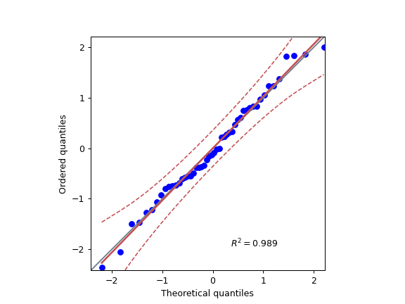
Two Q-Q plots using two separate axes:
\>>> import numpy as np
\>>> import pingouin as pg
\>>> import matplotlib.pyplot as plt
\>>> np.random.seed(123)
\>>> x \= np.random.normal(size\=50)
\>>> x\_exp \= np.random.exponential(size\=50)
\>>> fig, (ax1, ax2) \= plt.subplots(1, 2, figsize\=(9, 4))
\>>> ax1 \= pg.qqplot(x, dist\='norm', ax\=ax1, confidence\=False)
\>>> ax2 \= pg.qqplot(x\_exp, dist\='expon', ax\=ax2)
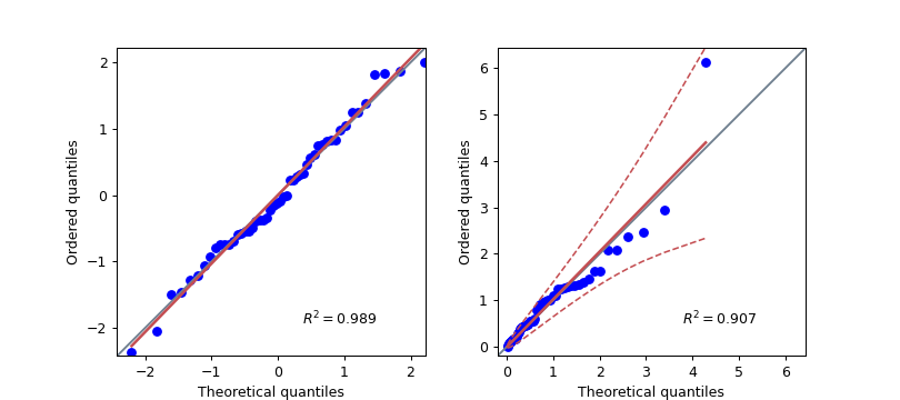
Using custom location / scale parameters as well as another Seaborn style
\>>> import numpy as np
\>>> import seaborn as sns
\>>> import pingouin as pg
\>>> import matplotlib.pyplot as plt
\>>> np.random.seed(123)
\>>> x \= np.random.normal(size\=50)
\>>> mean, std \= 0, 0.8
\>>> sns.set\_style('darkgrid')
\>>> ax \= pg.qqplot(x, dist\='norm', sparams\=(mean, std))

On this page
[Edit on GitHub](https://github.com/raphaelvallat/pingouin/edit/main/docs/generated/pingouin.qqplot.rst)
---
# pingouin.intraclass_corr — pingouin 0.5.5 documentation
[Skip to main content](https://pingouin-stats.org/build/html/generated/pingouin.intraclass_corr.html#main-content)
Back to top
Ctrl+K
* [GitHub](https://github.com/raphaelvallat/pingouin "GitHub")
pingouin.intraclass\_corr[#](https://pingouin-stats.org/build/html/generated/pingouin.intraclass_corr.html#pingouin-intraclass-corr "Link to this heading")
============================================================================================================================================================
pingouin.intraclass\_corr(_data\=None_, _targets\=None_, _raters\=None_, _ratings\=None_, _nan\_policy\='raise'_)[\[source\]](https://pingouin-stats.org/build/html/_modules/pingouin/reliability.html#intraclass_corr)
[#](https://pingouin-stats.org/build/html/generated/pingouin.intraclass_corr.html#pingouin.intraclass_corr "Link to this definition")
Intraclass correlation.
Parameters:
**data**[`pandas.DataFrame`](https://pandas.pydata.org/pandas-docs/stable/reference/api/pandas.DataFrame.html#pandas.DataFrame "(in pandas v2.2.2)")
Long-format dataframe. Data must be fully balanced.
**targets**string
Name of column in `data` containing the targets.
**raters**string
Name of column in `data` containing the raters.
**ratings**string
Name of column in `data` containing the ratings.
**nan\_policy**str
Defines how to handle when input contains missing values (nan). ‘raise’ (default) throws an error, ‘omit’ performs the calculations after deleting target(s) with one or more missing values (= listwise deletion).
Added in version 0.3.0.
Returns:
**stats**[`pandas.DataFrame`](https://pandas.pydata.org/pandas-docs/stable/reference/api/pandas.DataFrame.html#pandas.DataFrame "(in pandas v2.2.2)")
Output dataframe:
* `'Type'`: ICC type
* `'Description'`: description of the ICC
* `'ICC'`: intraclass correlation
* `'F'`: F statistic
* `'df1'`: numerator degree of freedom
* `'df2'`: denominator degree of freedom
* `'pval'`: p-value
* `'CI95%'`: 95% confidence intervals around the ICC
Notes
The intraclass correlation (ICC, [\[1\]](https://pingouin-stats.org/build/html/generated/pingouin.intraclass_corr.html#rc6e049bc6922-1)
) assesses the reliability of ratings by comparing the variability of different ratings of the same subject to the total variation across all ratings and all subjects.
Shrout and Fleiss (1979) [\[2\]](https://pingouin-stats.org/build/html/generated/pingouin.intraclass_corr.html#rc6e049bc6922-2)
describe six cases of reliability of ratings done by \\(k\\) raters on \\(n\\) targets. Pingouin returns all six cases with corresponding F and p-values, as well as 95% confidence intervals.
From the documentation of the ICC function in the [psych](https://cran.r-project.org/web/packages/psych/psych.pdf)
R package:
* **ICC1**: Each target is rated by a different rater and the raters are selected at random. This is a one-way ANOVA fixed effects model.
* **ICC2**: A random sample of \\(k\\) raters rate each target. The measure is one of absolute agreement in the ratings. ICC1 is sensitive to differences in means between raters and is a measure of absolute agreement.
* **ICC3**: A fixed set of \\(k\\) raters rate each target. There is no generalization to a larger population of raters. ICC2 and ICC3 remove mean differences between raters, but are sensitive to interactions. The difference between ICC2 and ICC3 is whether raters are seen as fixed or random effects.
Then, for each of these cases, the reliability can either be estimated for a single rating or for the average of \\(k\\) ratings. The 1 rating case is equivalent to the average intercorrelation, while the \\(k\\) rating case is equivalent to the Spearman Brown adjusted reliability. **ICC1k**, **ICC2k**, **ICC3K** reflect the means of \\(k\\) raters.
This function has been tested against the ICC function of the R psych package. Note however that contrarily to the R implementation, the current implementation does not use linear mixed effect but regular ANOVA, which means that it only works with complete-case data (no missing values).
References
\[[1](https://pingouin-stats.org/build/html/generated/pingouin.intraclass_corr.html#id1)\
\]
[http://www.real-statistics.com/reliability/intraclass-correlation/](http://www.real-statistics.com/reliability/intraclass-correlation/)
\[[2](https://pingouin-stats.org/build/html/generated/pingouin.intraclass_corr.html#id2)\
\]
Shrout, P. E., & Fleiss, J. L. (1979). Intraclass correlations: uses in assessing rater reliability. Psychological bulletin, 86(2), 420.
Examples
ICCs of wine quality assessed by 4 judges.
\>>> import pingouin as pg
\>>> data \= pg.read\_dataset('icc')
\>>> icc \= pg.intraclass\_corr(data\=data, targets\='Wine', raters\='Judge',
... ratings\='Scores').round(3)
\>>> icc.set\_index("Type")
Description ICC F df1 df2 pval CI95%
Type
ICC1 Single raters absolute 0.728 11.680 7 24 0.0 \[0.43, 0.93\]
ICC2 Single random raters 0.728 11.787 7 21 0.0 \[0.43, 0.93\]
ICC3 Single fixed raters 0.729 11.787 7 21 0.0 \[0.43, 0.93\]
ICC1k Average raters absolute 0.914 11.680 7 24 0.0 \[0.75, 0.98\]
ICC2k Average random raters 0.914 11.787 7 21 0.0 \[0.75, 0.98\]
ICC3k Average fixed raters 0.915 11.787 7 21 0.0 \[0.75, 0.98\]
On this page
[Edit on GitHub](https://github.com/raphaelvallat/pingouin/edit/main/docs/generated/pingouin.intraclass_corr.rst)
---