# Table of Contents
- [
Documentation page not found
- Read the Docs Community ](#-documentation-page-not-found-read-the-docs-community-)
- [User Guide — PyPortfolioOpt 1.4.1 documentation](#user-guide-pyportfolioopt-1-4-1-documentation)
- [Expected Returns — PyPortfolioOpt 1.4.1 documentation](#expected-returns-pyportfolioopt-1-4-1-documentation)
- [User Guide — PyPortfolioOpt 1.5.4 documentation](#user-guide-pyportfolioopt-1-5-4-documentation)
- [Expected Returns — PyPortfolioOpt 1.5.4 documentation](#expected-returns-pyportfolioopt-1-5-4-documentation)
- [Risk Models — PyPortfolioOpt 1.4.1 documentation](#risk-models-pyportfolioopt-1-4-1-documentation)
- [Installation — PyPortfolioOpt 1.4.1 documentation](#installation-pyportfolioopt-1-4-1-documentation)
- [Risk Models — PyPortfolioOpt 1.5.4 documentation](#risk-models-pyportfolioopt-1-5-4-documentation)
- [Installation — PyPortfolioOpt 1.5.4 documentation](#installation-pyportfolioopt-1-5-4-documentation)
- [Mean-Variance Optimization — PyPortfolioOpt 1.5.4 documentation](#mean-variance-optimization-pyportfolioopt-1-5-4-documentation)
- [Mean-Variance Optimization — PyPortfolioOpt 1.4.1 documentation](#mean-variance-optimization-pyportfolioopt-1-4-1-documentation)
- [Other Optimizers — PyPortfolioOpt 1.4.1 documentation](#other-optimizers-pyportfolioopt-1-4-1-documentation)
- [Post-processing weights — PyPortfolioOpt 1.4.1 documentation](#post-processing-weights-pyportfolioopt-1-4-1-documentation)
- [Other Optimizers — PyPortfolioOpt 1.5.4 documentation](#other-optimizers-pyportfolioopt-1-5-4-documentation)
- [Post-processing weights — PyPortfolioOpt 1.5.4 documentation](#post-processing-weights-pyportfolioopt-1-5-4-documentation)
- [Plotting — PyPortfolioOpt 1.5.4 documentation](#plotting-pyportfolioopt-1-5-4-documentation)
- [Plotting — PyPortfolioOpt 1.4.1 documentation](#plotting-pyportfolioopt-1-4-1-documentation)
- [Roadmap and Changelog — PyPortfolioOpt 1.4.1 documentation](#roadmap-and-changelog-pyportfolioopt-1-4-1-documentation)
- [FAQs — PyPortfolioOpt 1.5.4 documentation](#faqs-pyportfolioopt-1-5-4-documentation)
- [FAQs — PyPortfolioOpt 1.4.1 documentation](#faqs-pyportfolioopt-1-4-1-documentation)
- [Contributing — PyPortfolioOpt 1.4.1 documentation](#contributing-pyportfolioopt-1-4-1-documentation)
- [Roadmap and Changelog — PyPortfolioOpt 1.5.4 documentation](#roadmap-and-changelog-pyportfolioopt-1-5-4-documentation)
- [Citing PyPortfolioOpt — PyPortfolioOpt 1.5.4 documentation](#citing-pyportfolioopt-pyportfolioopt-1-5-4-documentation)
- [Contributing — PyPortfolioOpt 1.5.4 documentation](#contributing-pyportfolioopt-1-5-4-documentation)
- [Python Module Index — PyPortfolioOpt 1.5.4 documentation](#python-module-index-pyportfolioopt-1-5-4-documentation)
- [Search — PyPortfolioOpt 1.4.1 documentation](#search-pyportfolioopt-1-4-1-documentation)
- [About — PyPortfolioOpt 1.5.4 documentation](#about-pyportfolioopt-1-5-4-documentation)
- [About — PyPortfolioOpt 1.4.1 documentation](#about-pyportfolioopt-1-4-1-documentation)
- [Python Module Index — PyPortfolioOpt 1.4.1 documentation](#python-module-index-pyportfolioopt-1-4-1-documentation)
- [Search — PyPortfolioOpt 1.5.4 documentation](#search-pyportfolioopt-1-5-4-documentation)
- [Black-Litterman Allocation — PyPortfolioOpt 1.5.4 documentation](#black-litterman-allocation-pyportfolioopt-1-5-4-documentation)
- [Black-Litterman Allocation — PyPortfolioOpt 1.4.1 documentation](#black-litterman-allocation-pyportfolioopt-1-4-1-documentation)
- [General Efficient Frontier — PyPortfolioOpt 1.5.4 documentation](#general-efficient-frontier-pyportfolioopt-1-5-4-documentation)
- [General Efficient Frontier — PyPortfolioOpt 1.4.1 documentation](#general-efficient-frontier-pyportfolioopt-1-4-1-documentation)
- [Index — PyPortfolioOpt 1.5.4 documentation](#index-pyportfolioopt-1-5-4-documentation)
- [Index — PyPortfolioOpt 1.4.1 documentation](#index-pyportfolioopt-1-4-1-documentation)
---
#
Documentation page not found
- Read the Docs Community
[pyportfolioopt.readthedocs.io](https://pyportfolioopt.readthedocs.io/)
The documentation page you requested does not exist or may have been removed.
Hosted by [](https://app.readthedocs.org/)
---
# User Guide — PyPortfolioOpt 1.4.1 documentation
* [Docs](https://pyportfolioopt.readthedocs.io/en/stable/index.html)
»
* User Guide
* [Edit on GitHub](https://github.com/robertmartin8/PyPortfolioOpt/blob/1db089602dee348f1eade9b981ca21cd35f1dcca/docs/UserGuide.rst)
* * *
User Guide[¶](https://pyportfolioopt.readthedocs.io/en/stable/UserGuide.html#user-guide "Permalink to this headline")
======================================================================================================================
This is designed to be a practical guide, mostly aimed at users who are interested in a quick way of optimally combining some assets (most likely stocks). However, when necessary I do introduce the required theory and also point out areas that may be suitable springboards for more advanced optimization techniques. Details about the parameters can be found in the respective documentation pages (please see the sidebar).
For this guide, we will be focusing on mean-variance optimization (MVO), which is what most people think of when they hear “portfolio optimization”. MVO forms the core of PyPortfolioOpt’s offering, though it should be noted that MVO comes in many flavours, which can have very different performance characteristics. Please refer to the sidebar to get a feeling for the possibilities, as well as the other optimization methods offered. But for now, we will continue with the standard Efficient Frontier.
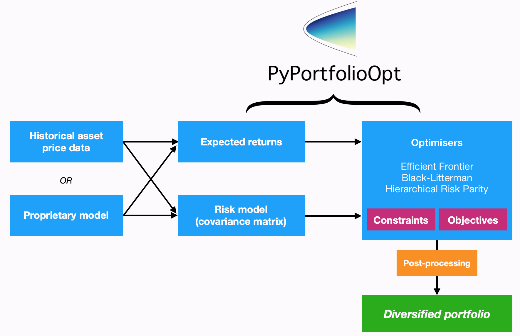
PyPortfolioOpt is designed with modularity in mind; the below flowchart sums up the current functionality and overall layout of PyPortfolioOpt.
Processing historical prices[¶](https://pyportfolioopt.readthedocs.io/en/stable/UserGuide.html#processing-historical-prices "Permalink to this headline")
----------------------------------------------------------------------------------------------------------------------------------------------------------
Mean-variance optimization requires two things: the expected returns of the assets, and the covariance matrix (or more generally, a _risk model_ quantifying asset risk). PyPortfolioOpt provides methods for estimating both (located in `expected_returns` and `risk_models` respectively), but also supports users who would like to use their own models.
However, I assume that most users will (at least initially) prefer to use the built-ins. In this case, all you need to supply is a dataset of historical prices for your assets. This dataset should look something like the one below:
XOM RRC BBY MA PFE JPM
date
2010\-01\-04 54.068794 51.300568 32.524055 22.062426 13.940202 35.175220
2010\-01\-05 54.279907 51.993038 33.349487 21.997149 13.741367 35.856571
2010\-01\-06 54.749043 51.690697 33.090542 22.081820 13.697187 36.053574
2010\-01\-07 54.577045 51.593170 33.616547 21.937523 13.645634 36.767757
2010\-01\-08 54.358093 52.597733 32.297466 21.945297 13.756095 36.677460
The index should consist of dates or timestamps, and each column should represent the time series of prices for an asset. A dataset of real-life stock prices has been included in the [tests folder](https://github.com/robertmartin8/PyPortfolioOpt/tree/master/tests)
of the GitHub repo.
Note
Pricing data does not have to be daily, but the frequency should be the same across all assets (workarounds exist but are not pretty).
After reading your historical prices into a pandas dataframe `df`, you need to decide between the available methods for estimating expected returns and the covariance matrix. Sensible defaults are `expected_returns.mean_historical_return()` and the Ledoit Wolf shrinkage estimate of the covariance matrix found in `risk_models.CovarianceShrinkage`. It is simply a matter of applying the relevant functions to the price dataset:
from pypfopt.expected\_returns import mean\_historical\_return
from pypfopt.risk\_models import CovarianceShrinkage
mu \= mean\_historical\_return(df)
S \= CovarianceShrinkage(df).ledoit\_wolf()
`mu` will then be a pandas series of estimated expected returns for each asset, and `S` will be the estimated covariance matrix (part of it is shown below):
GOOG AAPL FB BABA AMZN GE AMD \\
GOOG 0.045529 0.022143 0.006389 0.003720 0.026085 0.015815 0.021761
AAPL 0.022143 0.207037 0.004334 0.002954 0.058200 0.038102 0.084053
FB 0.006389 0.004334 0.029233 0.003770 0.007619 0.003008 0.005804
BABA 0.003720 0.002954 0.003770 0.013438 0.004176 0.002011 0.006332
AMZN 0.026085 0.058200 0.007619 0.004176 0.276365 0.038169 0.075657
GE 0.015815 0.038102 0.003008 0.002011 0.038169 0.083405 0.048580
AMD 0.021761 0.084053 0.005804 0.006332 0.075657 0.048580 0.388916
Now that we have expected returns and a risk model, we are ready to move on to the actual portfolio optimization.
Mean-variance optimization[¶](https://pyportfolioopt.readthedocs.io/en/stable/UserGuide.html#mean-variance-optimization "Permalink to this headline")
------------------------------------------------------------------------------------------------------------------------------------------------------
Mean-variance optimization is based on Harry Markowitz’s 1952 classic paper [\[1\]](https://pyportfolioopt.readthedocs.io/en/stable/UserGuide.html#id3)
, which spearheaded the transformation of portfolio management from an art into a science. The key insight is that by combining assets with different expected returns and volatilities, one can decide on a mathematically optimal allocation.
If \\(w\\) is the weight vector of stocks with expected returns \\(\\mu\\), then the portfolio return is equal to each stock’s weight multiplied by its return, i.e \\(w^T \\mu\\). The portfolio risk in terms of the covariance matrix \\(\\Sigma\\) is given by \\(w^T \\Sigma w\\). Portfolio optimization can then be regarded as a convex optimization problem, and a solution can be found using quadratic programming. If we denote the target return as \\(\\mu^\*\\), the precise statement of the long-only portfolio optimization problem is as follows:
\\\[\\begin{split}\\begin{equation\*} \\begin{aligned} & \\underset{w}{\\text{minimise}} & & w^T \\Sigma w \\\\ & \\text{subject to} & & w^T\\mu \\geq \\mu^\*\\\\ &&& w^T\\mathbf{1} = 1 \\\\ &&& w\_i \\geq 0 \\\\ \\end{aligned} \\end{equation\*}\\end{split}\\\]
If we vary the target return, we will get a different set of weights (i.e a different portfolio) – the set of all these optimal portfolios is referred to as the **efficient frontier**.
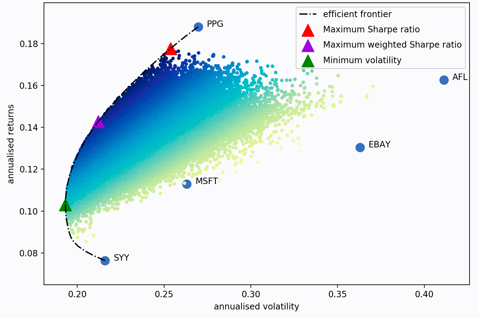
Each dot on this diagram represents a different possible portfolio, with darker blue corresponding to ‘better’ portfolios (in terms of the Sharpe Ratio). The dotted black line is the efficient frontier itself. The triangular markers represent the best portfolios for different optimization objectives.
The Sharpe ratio is the portfolio’s return in excess of the risk-free rate, per unit risk (volatility).
\\\[SR = \\frac{R\_P - R\_f}{\\sigma}\\\]
It is particularly important because it measures the portfolio returns, adjusted for risk. So in practice, rather than trying to minimise volatility for a given target return (as per Markowitz 1952), it often makes more sense to just find the portfolio that maximises the Sharpe ratio. This is implemented as the `max_sharpe()` method in the `EfficientFrontier` class. Using the series `mu` and dataframe `S` from before:
from pypfopt.efficient\_frontier import EfficientFrontier
ef \= EfficientFrontier(mu, S)
weights \= ef.max\_sharpe()
If you print these weights, you will get quite an ugly result, because they will be the raw output from the optimizer. As such, it is recommended that you use the `clean_weights()` method, which truncates tiny weights to zero and rounds the rest:
cleaned\_weights \= ef.clean\_weights()
ef.save\_weights\_to\_file("weights.txt") \# saves to file
print(cleaned\_weights)
This prints:
{'GOOG': 0.01269,
'AAPL': 0.09202,
'FB': 0.19856,
'BABA': 0.09642,
'AMZN': 0.07158,
'GE': 0.0,
'AMD': 0.0,
'WMT': 0.0,
'BAC': 0.0,
'GM': 0.0,
'T': 0.0,
'UAA': 0.0,
'SHLD': 0.0,
'XOM': 0.0,
'RRC': 0.0,
'BBY': 0.06129,
'MA': 0.24562,
'PFE': 0.18413,
'JPM': 0.0,
'SBUX': 0.03769}
If we want to know the expected performance of the portfolio with optimal weights `w`, we can use the `portfolio_performance()` method:
ef.portfolio\_performance(verbose\=True)
Expected annual return: 33.0%
Annual volatility: 21.7%
Sharpe Ratio: 1.43
A detailed discussion of optimization parameters is presented in [General Efficient Frontier](https://pyportfolioopt.readthedocs.io/en/stable/GeneralEfficientFrontier.html#efficient-frontier)
. However, there are two main variations which are discussed below.
### Short positions[¶](https://pyportfolioopt.readthedocs.io/en/stable/UserGuide.html#short-positions "Permalink to this headline")
To allow for shorting, simply initialise the `EfficientFrontier` object with bounds that allow negative weights, for example:
ef \= EfficientFrontier(mu, S, weight\_bounds\=(\-1,1))
This can be extended to generate **market neutral portfolios** (with weights summing to zero), but these are only available for the `efficient_risk()` and `efficient_return()` optimization methods for mathematical reasons. If you want a market neutral portfolio, pass `market_neutral=True` as shown below:
ef.efficient\_return(target\_return\=0.2, market\_neutral\=True)
### Dealing with many negligible weights[¶](https://pyportfolioopt.readthedocs.io/en/stable/UserGuide.html#dealing-with-many-negligible-weights "Permalink to this headline")
From experience, I have found that mean-variance optimization often sets many of the asset weights to be zero. This may not be ideal if you need to have a certain number of positions in your portfolio, for diversification purposes or otherwise.
To combat this, I have introduced an objective function which borrows the idea of regularisation from machine learning. Essentially, by adding an additional cost function to the objective, you can ‘encourage’ the optimizer to choose different weights (mathematical details are provided in the [More on L2 Regularisation](https://pyportfolioopt.readthedocs.io/en/stable/MeanVariance.html#l2-regularisation)
section). To use this feature, change the `gamma` parameter:
from pypfopt import objective\_functions
ef \= EfficientFrontier(mu, S)
ef.add\_objective(objective\_functions.L2\_reg, gamma\=0.1)
w \= ef.max\_sharpe()
print(ef.clean\_weights())
The result of this has far fewer negligible weights than before:
{'GOOG': 0.06366,
'AAPL': 0.09947,
'FB': 0.15742,
'BABA': 0.08701,
'AMZN': 0.09454,
'GE': 0.0,
'AMD': 0.0,
'WMT': 0.01766,
'BAC': 0.0,
'GM': 0.0,
'T': 0.00398,
'UAA': 0.0,
'SHLD': 0.0,
'XOM': 0.03072,
'RRC': 0.00737,
'BBY': 0.07572,
'MA': 0.1769,
'PFE': 0.12346,
'JPM': 0.0,
'SBUX': 0.06209}
### Post-processing weights[¶](https://pyportfolioopt.readthedocs.io/en/stable/UserGuide.html#post-processing-weights "Permalink to this headline")
In practice, we then need to convert these weights into an actual allocation, telling you how many shares of each asset you should purchase. This is discussed further in [Post-processing weights](https://pyportfolioopt.readthedocs.io/en/stable/Postprocessing.html#post-processing)
, but we provide an example below:
from pypfopt.discrete\_allocation import DiscreteAllocation, get\_latest\_prices
latest\_prices \= get\_latest\_prices(df)
da \= DiscreteAllocation(w, latest\_prices, total\_portfolio\_value\=20000)
allocation, leftover \= da.lp\_portfolio()
print(allocation)
These are the quantities of shares that should be bought to have a $20,000 portfolio:
{'AAPL': 2.0,
'FB': 12.0,
'BABA': 14.0,
'GE': 18.0,
'WMT': 40.0,
'GM': 58.0,
'T': 97.0,
'SHLD': 1.0,
'XOM': 47.0,
'RRC': 3.0,
'BBY': 1.0,
'PFE': 47.0,
'SBUX': 5.0}
Improving performance[¶](https://pyportfolioopt.readthedocs.io/en/stable/UserGuide.html#improving-performance "Permalink to this headline")
--------------------------------------------------------------------------------------------------------------------------------------------
Let’s say you have conducted backtests and the results aren’t spectacular. What should you try?
* Try the Hierarchical Risk Parity model (see [Other Optimizers](https://pyportfolioopt.readthedocs.io/en/stable/OtherOptimizers.html#other-optimizers)
) – which seems to robustly outperform mean-variance optimization out of sample.
* Use the Black-Litterman model to construct a more stable model of expected returns. Alternatively, just drop the expected returns altogether! There is a large body of research that suggests that minimum variance portfolios (`ef.min_volatility()`) consistently outperform maximum Sharpe ratio portfolios out-of-sample (even when measured by Sharpe ratio), because of the difficulty of forecasting expected returns.
* Try different risk models: shrinkage models are known to have better numerical properties compared with the sample covariance matrix.
* Add some new objective terms or constraints. Tune the L2 regularisation parameter to see how diversification affects the performance.
This concludes the guided tour. Head over to the appropriate sections in the sidebar to learn more about the parameters and theoretical details of the different models offered by PyPortfolioOpt. If you have any questions, please raise an issue on GitHub and I will try to respond promptly.
If you’d like even more examples, check out the cookbook [recipe](https://github.com/robertmartin8/PyPortfolioOpt/blob/master/cookbook/2-Mean-Variance-Optimization.ipynb)
.
References[¶](https://pyportfolioopt.readthedocs.io/en/stable/UserGuide.html#references "Permalink to this headline")
----------------------------------------------------------------------------------------------------------------------
| | |
| --- | --- |
| [\[1\]](https://pyportfolioopt.readthedocs.io/en/stable/UserGuide.html#id2) | Markowitz, H. (1952). [Portfolio Selection](https://onlinelibrary.wiley.com/doi/abs/10.1111/j.1540-6261.1952.tb01525.x)
. The Journal of Finance, 7(1), 77–91. [https://doi.org/10.1111/j.1540-6261.1952.tb01525.x](https://doi.org/10.1111/j.1540-6261.1952.tb01525.x) |
---
# Expected Returns — PyPortfolioOpt 1.4.1 documentation
* [Docs](https://pyportfolioopt.readthedocs.io/en/stable/index.html)
»
* Expected Returns
* [Edit on GitHub](https://github.com/robertmartin8/PyPortfolioOpt/blob/1db089602dee348f1eade9b981ca21cd35f1dcca/docs/ExpectedReturns.rst)
* * *
Expected Returns[¶](https://pyportfolioopt.readthedocs.io/en/stable/ExpectedReturns.html#expected-returns "Permalink to this headline")
========================================================================================================================================
Mean-variance optimization requires knowledge of the expected returns. In practice, these are rather difficult to know with any certainty. Thus the best we can do is to come up with estimates, for example by extrapolating historical data, This is the main flaw in mean-variance optimization – the optimization procedure is sound, and provides strong mathematical guarantees, _given the correct inputs_. This is one of the reasons why I have emphasised modularity: users should be able to come up with their own superior models and feed them into the optimizer.
Caution
Supplying expected returns can do more harm than good. If predicting stock returns were as easy as calculating the mean historical return, we’d all be rich! For most use-cases, I would suggest that you focus your efforts on choosing an appropriate risk model (see [Risk Models](https://pyportfolioopt.readthedocs.io/en/stable/RiskModels.html#risk-models)
).
As of v0.5.0, you can use [Black-Litterman Allocation](https://pyportfolioopt.readthedocs.io/en/stable/BlackLitterman.html#black-litterman)
to significantly improve the quality of your estimate of the expected returns.
The `expected_returns` module provides functions for estimating the expected returns of the assets, which is a required input in mean-variance optimization.
By convention, the output of these methods is expected _annual_ returns. It is assumed that _daily_ prices are provided, though in reality the functions are agnostic to the time period (just change the `frequency` parameter). Asset prices must be given as a pandas dataframe, as per the format described in the [User Guide](https://pyportfolioopt.readthedocs.io/en/stable/UserGuide.html#user-guide)
.
All of the functions process the price data into percentage returns data, before calculating their respective estimates of expected returns.
Currently implemented:
> * general return model function, allowing you to run any return model from one function.
> * mean historical return
> * exponentially weighted mean historical return
> * CAPM estimate of returns
Additionally, we provide utility functions to convert from returns to prices and vice-versa.
Note
For any of these methods, if you would prefer to pass returns (the default is prices), set the boolean flag `returns_data=True`
`pypfopt.expected_returns.``mean_historical_return`(_prices_, _returns\_data=False_, _compounding=True_, _frequency=252_)[\[source\]](https://pyportfolioopt.readthedocs.io/en/stable/_modules/pypfopt/expected_returns.html#mean_historical_return)
[¶](https://pyportfolioopt.readthedocs.io/en/stable/ExpectedReturns.html#pypfopt.expected_returns.mean_historical_return "Permalink to this definition")
Calculate annualised mean (daily) historical return from input (daily) asset prices. Use `compounding` to toggle between the default geometric mean (CAGR) and the arithmetic mean.
| | |
| --- | --- |
| Parameters: | * **prices** (_pd.DataFrame_) – adjusted closing prices of the asset, each row is a date and each column is a ticker/id.
* **returns\_data** (_bool__,_ _defaults to False._) – if true, the first argument is returns instead of prices. These **should not** be log returns.
* **compounding** (_bool__,_ _defaults to True_) – computes geometric mean returns if True, arithmetic otherwise, optional.
* **frequency** (_int__,_ _optional_) – number of time periods in a year, defaults to 252 (the number of trading days in a year) |
| Returns: | annualised mean (daily) return for each asset |
| Return type: | pd.Series |
This is probably the default textbook approach. It is intuitive and easily interpretable, however the estimates are subject to large uncertainty. This is a problem especially in the context of a mean-variance optimizer, which will maximise the erroneous inputs.
`pypfopt.expected_returns.``ema_historical_return`(_prices_, _returns\_data=False_, _compounding=True_, _span=500_, _frequency=252_)[\[source\]](https://pyportfolioopt.readthedocs.io/en/stable/_modules/pypfopt/expected_returns.html#ema_historical_return)
[¶](https://pyportfolioopt.readthedocs.io/en/stable/ExpectedReturns.html#pypfopt.expected_returns.ema_historical_return "Permalink to this definition")
Calculate the exponentially-weighted mean of (daily) historical returns, giving higher weight to more recent data.
| | |
| --- | --- |
| Parameters: | * **prices** (_pd.DataFrame_) – adjusted closing prices of the asset, each row is a date and each column is a ticker/id.
* **returns\_data** (_bool__,_ _defaults to False._) – if true, the first argument is returns instead of prices. These **should not** be log returns.
* **compounding** (_bool__,_ _defaults to True_) – computes geometric mean returns if True, arithmetic otherwise, optional.
* **frequency** (_int__,_ _optional_) – number of time periods in a year, defaults to 252 (the number of trading days in a year)
* **span** (_int__,_ _optional_) – the time-span for the EMA, defaults to 500-day EMA. |
| Returns: | annualised exponentially-weighted mean (daily) return of each asset |
| Return type: | pd.Series |
The exponential moving average is a simple improvement over the mean historical return; it gives more credence to recent returns and thus aims to increase the relevance of the estimates. This is parameterised by the `span` parameter, which gives users the ability to decide exactly how much more weight is given to recent data. Generally, I would err on the side of a higher span – in the limit, this tends towards the mean historical return. However, if you plan on rebalancing much more frequently, there is a case to be made for lowering the span in order to capture recent trends.
`pypfopt.expected_returns.``capm_return`(_prices_, _market\_prices=None_, _returns\_data=False_, _risk\_free\_rate=0.02_, _compounding=True_, _frequency=252_)[\[source\]](https://pyportfolioopt.readthedocs.io/en/stable/_modules/pypfopt/expected_returns.html#capm_return)
[¶](https://pyportfolioopt.readthedocs.io/en/stable/ExpectedReturns.html#pypfopt.expected_returns.capm_return "Permalink to this definition")
Compute a return estimate using the Capital Asset Pricing Model. Under the CAPM, asset returns are equal to market returns plus a \\(�eta\\) term encoding the relative risk of the asset.
\\\[R\_i = R\_f + \\beta\_i (E(R\_m) - R\_f)\\\]
| | |
| --- | --- |
| Parameters: | * **prices** (_pd.DataFrame_) – adjusted closing prices of the asset, each row is a date and each column is a ticker/id.
* **market\_prices** (_pd.DataFrame__,_ _optional_) – adjusted closing prices of the benchmark, defaults to None
* **returns\_data** (_bool__,_ _defaults to False._) – if true, the first arguments are returns instead of prices.
* **risk\_free\_rate** (_float__,_ _optional_) – risk-free rate of borrowing/lending, defaults to 0.02. You should use the appropriate time period, corresponding to the frequency parameter.
* **compounding** (_bool__,_ _defaults to True_) – computes geometric mean returns if True, arithmetic otherwise, optional.
* **frequency** (_int__,_ _optional_) – number of time periods in a year, defaults to 252 (the number of trading days in a year) |
| Returns: | annualised return estimate |
| Return type: | pd.Series |
`pypfopt.expected_returns.``returns_from_prices`(_prices_, _log\_returns=False_)[\[source\]](https://pyportfolioopt.readthedocs.io/en/stable/_modules/pypfopt/expected_returns.html#returns_from_prices)
[¶](https://pyportfolioopt.readthedocs.io/en/stable/ExpectedReturns.html#pypfopt.expected_returns.returns_from_prices "Permalink to this definition")
Calculate the returns given prices.
| | |
| --- | --- |
| Parameters: | * **prices** (_pd.DataFrame_) – adjusted (daily) closing prices of the asset, each row is a date and each column is a ticker/id.
* **log\_returns** (_bool__,_ _defaults to False_) – whether to compute using log returns |
| Returns: | (daily) returns |
| Return type: | pd.DataFrame |
`pypfopt.expected_returns.``prices_from_returns`(_returns_, _log\_returns=False_)[\[source\]](https://pyportfolioopt.readthedocs.io/en/stable/_modules/pypfopt/expected_returns.html#prices_from_returns)
[¶](https://pyportfolioopt.readthedocs.io/en/stable/ExpectedReturns.html#pypfopt.expected_returns.prices_from_returns "Permalink to this definition")
Calculate the pseudo-prices given returns. These are not true prices because the initial prices are all set to 1, but it behaves as intended when passed to any PyPortfolioOpt method.
| | |
| --- | --- |
| Parameters: | * **returns** (_pd.DataFrame_) – (daily) percentage returns of the assets
* **log\_returns** (_bool__,_ _defaults to False_) – whether to compute using log returns |
| Returns: | (daily) pseudo-prices. |
| Return type: | pd.DataFrame |
---
# User Guide — PyPortfolioOpt 1.5.4 documentation
* [Docs](https://pyportfolioopt.readthedocs.io/en/latest/index.html)
»
* User Guide
* [Edit on GitHub](https://github.com/robertmartin8/PyPortfolioOpt/blob/master/docs/UserGuide.rst)
* * *
User Guide[¶](https://pyportfolioopt.readthedocs.io/en/latest/UserGuide.html#user-guide "Permalink to this headline")
======================================================================================================================
This is designed to be a practical guide, mostly aimed at users who are interested in a quick way of optimally combining some assets (most likely stocks). However, when necessary I do introduce the required theory and also point out areas that may be suitable springboards for more advanced optimization techniques. Details about the parameters can be found in the respective documentation pages (please see the sidebar).
For this guide, we will be focusing on mean-variance optimization (MVO), which is what most people think of when they hear “portfolio optimization”. MVO forms the core of PyPortfolioOpt’s offering, though it should be noted that MVO comes in many flavours, which can have very different performance characteristics. Please refer to the sidebar to get a feeling for the possibilities, as well as the other optimization methods offered. But for now, we will continue with the standard Efficient Frontier.
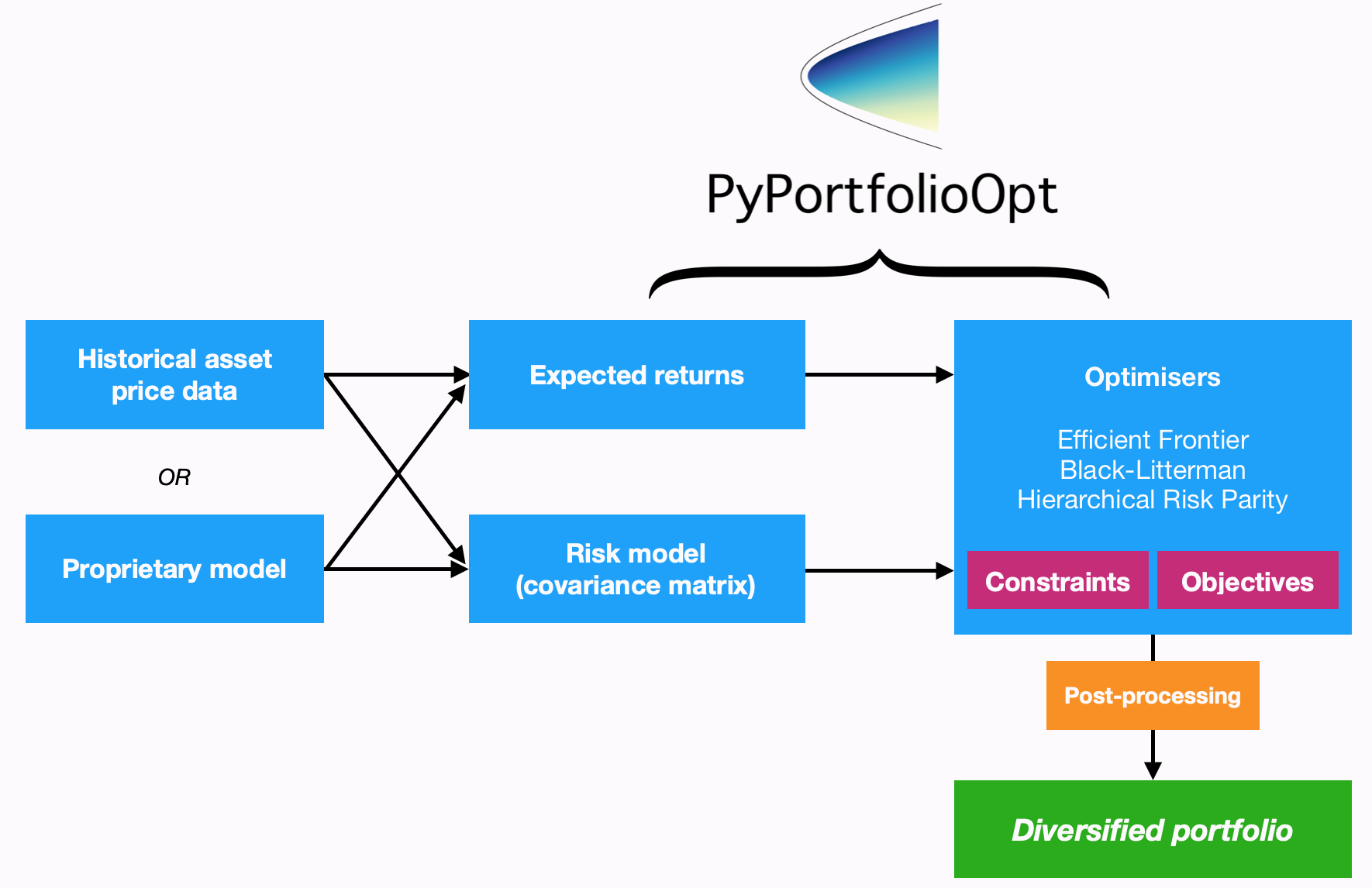
PyPortfolioOpt is designed with modularity in mind; the below flowchart sums up the current functionality and overall layout of PyPortfolioOpt.
Processing historical prices[¶](https://pyportfolioopt.readthedocs.io/en/latest/UserGuide.html#processing-historical-prices "Permalink to this headline")
----------------------------------------------------------------------------------------------------------------------------------------------------------
Mean-variance optimization requires two things: the expected returns of the assets, and the covariance matrix (or more generally, a _risk model_ quantifying asset risk). PyPortfolioOpt provides methods for estimating both (located in `expected_returns` and `risk_models` respectively), but also supports users who would like to use their own models.
However, I assume that most users will (at least initially) prefer to use the built-ins. In this case, all you need to supply is a dataset of historical prices for your assets. This dataset should look something like the one below:
XOM RRC BBY MA PFE JPM
date
2010\-01\-04 54.068794 51.300568 32.524055 22.062426 13.940202 35.175220
2010\-01\-05 54.279907 51.993038 33.349487 21.997149 13.741367 35.856571
2010\-01\-06 54.749043 51.690697 33.090542 22.081820 13.697187 36.053574
2010\-01\-07 54.577045 51.593170 33.616547 21.937523 13.645634 36.767757
2010\-01\-08 54.358093 52.597733 32.297466 21.945297 13.756095 36.677460
The index should consist of dates or timestamps, and each column should represent the time series of prices for an asset. A dataset of real-life stock prices has been included in the [tests folder](https://github.com/robertmartin8/PyPortfolioOpt/tree/master/tests)
of the GitHub repo.
Note
Pricing data does not have to be daily, but the frequency should be the same across all assets (workarounds exist but are not pretty).
After reading your historical prices into a pandas dataframe `df`, you need to decide between the available methods for estimating expected returns and the covariance matrix. Sensible defaults are `expected_returns.mean_historical_return()` and the Ledoit Wolf shrinkage estimate of the covariance matrix found in `risk_models.CovarianceShrinkage`. It is simply a matter of applying the relevant functions to the price dataset:
from pypfopt.expected\_returns import mean\_historical\_return
from pypfopt.risk\_models import CovarianceShrinkage
mu \= mean\_historical\_return(df)
S \= CovarianceShrinkage(df).ledoit\_wolf()
`mu` will then be a pandas series of estimated expected returns for each asset, and `S` will be the estimated covariance matrix (part of it is shown below):
GOOG AAPL FB BABA AMZN GE AMD \\
GOOG 0.045529 0.022143 0.006389 0.003720 0.026085 0.015815 0.021761
AAPL 0.022143 0.207037 0.004334 0.002954 0.058200 0.038102 0.084053
FB 0.006389 0.004334 0.029233 0.003770 0.007619 0.003008 0.005804
BABA 0.003720 0.002954 0.003770 0.013438 0.004176 0.002011 0.006332
AMZN 0.026085 0.058200 0.007619 0.004176 0.276365 0.038169 0.075657
GE 0.015815 0.038102 0.003008 0.002011 0.038169 0.083405 0.048580
AMD 0.021761 0.084053 0.005804 0.006332 0.075657 0.048580 0.388916
Now that we have expected returns and a risk model, we are ready to move on to the actual portfolio optimization.
Mean-variance optimization[¶](https://pyportfolioopt.readthedocs.io/en/latest/UserGuide.html#mean-variance-optimization "Permalink to this headline")
------------------------------------------------------------------------------------------------------------------------------------------------------
Mean-variance optimization is based on Harry Markowitz’s 1952 classic paper [\[1\]](https://pyportfolioopt.readthedocs.io/en/latest/UserGuide.html#id3)
, which spearheaded the transformation of portfolio management from an art into a science. The key insight is that by combining assets with different expected returns and volatilities, one can decide on a mathematically optimal allocation.
If \\(w\\) is the weight vector of stocks with expected returns \\(\\mu\\), then the portfolio return is equal to each stock’s weight multiplied by its return, i.e \\(w^T \\mu\\). The portfolio risk in terms of the covariance matrix \\(\\Sigma\\) is given by \\(w^T \\Sigma w\\). Portfolio optimization can then be regarded as a convex optimization problem, and a solution can be found using quadratic programming. If we denote the target return as \\(\\mu^\*\\), the precise statement of the long-only portfolio optimization problem is as follows:
\\\[\\begin{split}\\begin{equation\*} \\begin{aligned} & \\underset{w}{\\text{minimise}} & & w^T \\Sigma w \\\\ & \\text{subject to} & & w^T\\mu \\geq \\mu^\*\\\\ &&& w^T\\mathbf{1} = 1 \\\\ &&& w\_i \\geq 0 \\\\ \\end{aligned} \\end{equation\*}\\end{split}\\\]
If we vary the target return, we will get a different set of weights (i.e a different portfolio) – the set of all these optimal portfolios is referred to as the **efficient frontier**.
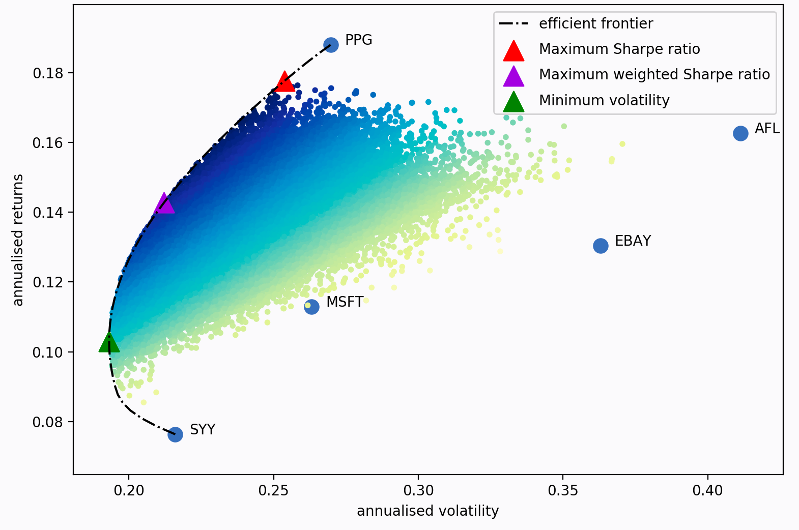
Each dot on this diagram represents a different possible portfolio, with darker blue corresponding to ‘better’ portfolios (in terms of the Sharpe Ratio). The dotted black line is the efficient frontier itself. The triangular markers represent the best portfolios for different optimization objectives.
The Sharpe ratio is the portfolio’s return in excess of the risk-free rate, per unit risk (volatility).
\\\[SR = \\frac{R\_P - R\_f}{\\sigma}\\\]
It is particularly important because it measures the portfolio returns, adjusted for risk. So in practice, rather than trying to minimise volatility for a given target return (as per Markowitz 1952), it often makes more sense to just find the portfolio that maximises the Sharpe ratio. This is implemented as the `max_sharpe()` method in the `EfficientFrontier` class. Using the series `mu` and dataframe `S` from before:
from pypfopt.efficient\_frontier import EfficientFrontier
ef \= EfficientFrontier(mu, S)
weights \= ef.max\_sharpe()
If you print these weights, you will get quite an ugly result, because they will be the raw output from the optimizer. As such, it is recommended that you use the `clean_weights()` method, which truncates tiny weights to zero and rounds the rest:
cleaned\_weights \= ef.clean\_weights()
ef.save\_weights\_to\_file("weights.txt") \# saves to file
print(cleaned\_weights)
This prints:
{'GOOG': 0.01269,
'AAPL': 0.09202,
'FB': 0.19856,
'BABA': 0.09642,
'AMZN': 0.07158,
'GE': 0.0,
'AMD': 0.0,
'WMT': 0.0,
'BAC': 0.0,
'GM': 0.0,
'T': 0.0,
'UAA': 0.0,
'SHLD': 0.0,
'XOM': 0.0,
'RRC': 0.0,
'BBY': 0.06129,
'MA': 0.24562,
'PFE': 0.18413,
'JPM': 0.0,
'SBUX': 0.03769}
If we want to know the expected performance of the portfolio with optimal weights `w`, we can use the `portfolio_performance()` method:
ef.portfolio\_performance(verbose\=True)
Expected annual return: 33.0%
Annual volatility: 21.7%
Sharpe Ratio: 1.43
A detailed discussion of optimization parameters is presented in [General Efficient Frontier](https://pyportfolioopt.readthedocs.io/en/latest/GeneralEfficientFrontier.html#efficient-frontier)
. However, there are two main variations which are discussed below.
### Short positions[¶](https://pyportfolioopt.readthedocs.io/en/latest/UserGuide.html#short-positions "Permalink to this headline")
To allow for shorting, simply initialise the `EfficientFrontier` object with bounds that allow negative weights, for example:
ef \= EfficientFrontier(mu, S, weight\_bounds\=(\-1,1))
This can be extended to generate **market neutral portfolios** (with weights summing to zero), but these are only available for the `efficient_risk()` and `efficient_return()` optimization methods for mathematical reasons. If you want a market neutral portfolio, pass `market_neutral=True` as shown below:
ef.efficient\_return(target\_return\=0.2, market\_neutral\=True)
### Dealing with many negligible weights[¶](https://pyportfolioopt.readthedocs.io/en/latest/UserGuide.html#dealing-with-many-negligible-weights "Permalink to this headline")
From experience, I have found that mean-variance optimization often sets many of the asset weights to be zero. This may not be ideal if you need to have a certain number of positions in your portfolio, for diversification purposes or otherwise.
To combat this, I have introduced an objective function which borrows the idea of regularisation from machine learning. Essentially, by adding an additional cost function to the objective, you can ‘encourage’ the optimizer to choose different weights (mathematical details are provided in the [More on L2 Regularisation](https://pyportfolioopt.readthedocs.io/en/latest/MeanVariance.html#l2-regularisation)
section). To use this feature, change the `gamma` parameter:
from pypfopt import objective\_functions
ef \= EfficientFrontier(mu, S)
ef.add\_objective(objective\_functions.L2\_reg, gamma\=0.1)
w \= ef.max\_sharpe()
print(ef.clean\_weights())
The result of this has far fewer negligible weights than before:
{'GOOG': 0.06366,
'AAPL': 0.09947,
'FB': 0.15742,
'BABA': 0.08701,
'AMZN': 0.09454,
'GE': 0.0,
'AMD': 0.0,
'WMT': 0.01766,
'BAC': 0.0,
'GM': 0.0,
'T': 0.00398,
'UAA': 0.0,
'SHLD': 0.0,
'XOM': 0.03072,
'RRC': 0.00737,
'BBY': 0.07572,
'MA': 0.1769,
'PFE': 0.12346,
'JPM': 0.0,
'SBUX': 0.06209}
### Post-processing weights[¶](https://pyportfolioopt.readthedocs.io/en/latest/UserGuide.html#post-processing-weights "Permalink to this headline")
In practice, we then need to convert these weights into an actual allocation, telling you how many shares of each asset you should purchase. This is discussed further in [Post-processing weights](https://pyportfolioopt.readthedocs.io/en/latest/Postprocessing.html#post-processing)
, but we provide an example below:
from pypfopt.discrete\_allocation import DiscreteAllocation, get\_latest\_prices
latest\_prices \= get\_latest\_prices(df)
da \= DiscreteAllocation(w, latest\_prices, total\_portfolio\_value\=20000)
allocation, leftover \= da.lp\_portfolio()
print(allocation)
These are the quantities of shares that should be bought to have a $20,000 portfolio:
{'AAPL': 2.0,
'FB': 12.0,
'BABA': 14.0,
'GE': 18.0,
'WMT': 40.0,
'GM': 58.0,
'T': 97.0,
'SHLD': 1.0,
'XOM': 47.0,
'RRC': 3.0,
'BBY': 1.0,
'PFE': 47.0,
'SBUX': 5.0}
Improving performance[¶](https://pyportfolioopt.readthedocs.io/en/latest/UserGuide.html#improving-performance "Permalink to this headline")
--------------------------------------------------------------------------------------------------------------------------------------------
Let’s say you have conducted backtests and the results aren’t spectacular. What should you try?
* Try the Hierarchical Risk Parity model (see [Other Optimizers](https://pyportfolioopt.readthedocs.io/en/latest/OtherOptimizers.html#other-optimizers)
) – which seems to robustly outperform mean-variance optimization out of sample.
* Use the Black-Litterman model to construct a more stable model of expected returns. Alternatively, just drop the expected returns altogether! There is a large body of research that suggests that minimum variance portfolios (`ef.min_volatility()`) consistently outperform maximum Sharpe ratio portfolios out-of-sample (even when measured by Sharpe ratio), because of the difficulty of forecasting expected returns.
* Try different risk models: shrinkage models are known to have better numerical properties compared with the sample covariance matrix.
* Add some new objective terms or constraints. Tune the L2 regularisation parameter to see how diversification affects the performance.
This concludes the guided tour. Head over to the appropriate sections in the sidebar to learn more about the parameters and theoretical details of the different models offered by PyPortfolioOpt. If you have any questions, please raise an issue on GitHub and I will try to respond promptly.
If you’d like even more examples, check out the cookbook [recipe](https://github.com/robertmartin8/PyPortfolioOpt/blob/master/cookbook/2-Mean-Variance-Optimization.ipynb)
.
References[¶](https://pyportfolioopt.readthedocs.io/en/latest/UserGuide.html#references "Permalink to this headline")
----------------------------------------------------------------------------------------------------------------------
| | |
| --- | --- |
| [\[1\]](https://pyportfolioopt.readthedocs.io/en/latest/UserGuide.html#id2) | Markowitz, H. (1952). [Portfolio Selection](https://onlinelibrary.wiley.com/doi/abs/10.1111/j.1540-6261.1952.tb01525.x)
. The Journal of Finance, 7(1), 77–91. [https://doi.org/10.1111/j.1540-6261.1952.tb01525.x](https://doi.org/10.1111/j.1540-6261.1952.tb01525.x) |
---
# Expected Returns — PyPortfolioOpt 1.5.4 documentation
* [Docs](https://pyportfolioopt.readthedocs.io/en/latest/index.html)
»
* Expected Returns
* [Edit on GitHub](https://github.com/robertmartin8/PyPortfolioOpt/blob/master/docs/ExpectedReturns.rst)
* * *
Expected Returns[¶](https://pyportfolioopt.readthedocs.io/en/latest/ExpectedReturns.html#expected-returns "Permalink to this headline")
========================================================================================================================================
Mean-variance optimization requires knowledge of the expected returns. In practice, these are rather difficult to know with any certainty. Thus the best we can do is to come up with estimates, for example by extrapolating historical data, This is the main flaw in mean-variance optimization – the optimization procedure is sound, and provides strong mathematical guarantees, _given the correct inputs_. This is one of the reasons why I have emphasised modularity: users should be able to come up with their own superior models and feed them into the optimizer.
Caution
Supplying expected returns can do more harm than good. If predicting stock returns were as easy as calculating the mean historical return, we’d all be rich! For most use-cases, I would suggest that you focus your efforts on choosing an appropriate risk model (see [Risk Models](https://pyportfolioopt.readthedocs.io/en/latest/RiskModels.html#risk-models)
).
As of v0.5.0, you can use [Black-Litterman Allocation](https://pyportfolioopt.readthedocs.io/en/latest/BlackLitterman.html#black-litterman)
to significantly improve the quality of your estimate of the expected returns.
The `expected_returns` module provides functions for estimating the expected returns of the assets, which is a required input in mean-variance optimization.
By convention, the output of these methods is expected _annual_ returns. It is assumed that _daily_ prices are provided, though in reality the functions are agnostic to the time period (just change the `frequency` parameter). Asset prices must be given as a pandas dataframe, as per the format described in the [User Guide](https://pyportfolioopt.readthedocs.io/en/latest/UserGuide.html#user-guide)
.
All of the functions process the price data into percentage returns data, before calculating their respective estimates of expected returns.
Currently implemented:
> * general return model function, allowing you to run any return model from one function.
> * mean historical return
> * exponentially weighted mean historical return
> * CAPM estimate of returns
Additionally, we provide utility functions to convert from returns to prices and vice-versa.
Note
For any of these methods, if you would prefer to pass returns (the default is prices), set the boolean flag `returns_data=True`
`pypfopt.expected_returns.``mean_historical_return`(_prices_, _returns\_data=False_, _compounding=True_, _frequency=252_, _log\_returns=False_)[\[source\]](https://pyportfolioopt.readthedocs.io/en/latest/_modules/pypfopt/expected_returns.html#mean_historical_return)
[¶](https://pyportfolioopt.readthedocs.io/en/latest/ExpectedReturns.html#pypfopt.expected_returns.mean_historical_return "Permalink to this definition")
Calculate annualised mean (daily) historical return from input (daily) asset prices. Use `compounding` to toggle between the default geometric mean (CAGR) and the arithmetic mean.
| | |
| --- | --- |
| Parameters: | * **prices** (_pd.DataFrame_) – adjusted closing prices of the asset, each row is a date and each column is a ticker/id.
* **returns\_data** (_bool__,_ _defaults to False._) – if true, the first argument is returns instead of prices. These **should not** be log returns.
* **compounding** (_bool__,_ _defaults to True_) – computes geometric mean returns if True, arithmetic otherwise, optional.
* **frequency** (_int__,_ _optional_) – number of time periods in a year, defaults to 252 (the number of trading days in a year)
* **log\_returns** (_bool__,_ _defaults to False_) – whether to compute using log returns |
| Returns: | annualised mean (daily) return for each asset |
| Return type: | pd.Series |
This is probably the default textbook approach. It is intuitive and easily interpretable, however the estimates are subject to large uncertainty. This is a problem especially in the context of a mean-variance optimizer, which will maximise the erroneous inputs.
`pypfopt.expected_returns.``ema_historical_return`(_prices_, _returns\_data=False_, _compounding=True_, _span=500_, _frequency=252_, _log\_returns=False_)[\[source\]](https://pyportfolioopt.readthedocs.io/en/latest/_modules/pypfopt/expected_returns.html#ema_historical_return)
[¶](https://pyportfolioopt.readthedocs.io/en/latest/ExpectedReturns.html#pypfopt.expected_returns.ema_historical_return "Permalink to this definition")
Calculate the exponentially-weighted mean of (daily) historical returns, giving higher weight to more recent data.
| | |
| --- | --- |
| Parameters: | * **prices** (_pd.DataFrame_) – adjusted closing prices of the asset, each row is a date and each column is a ticker/id.
* **returns\_data** (_bool__,_ _defaults to False._) – if true, the first argument is returns instead of prices. These **should not** be log returns.
* **compounding** (_bool__,_ _defaults to True_) – computes geometric mean returns if True, arithmetic otherwise, optional.
* **frequency** (_int__,_ _optional_) – number of time periods in a year, defaults to 252 (the number of trading days in a year)
* **span** (_int__,_ _optional_) – the time-span for the EMA, defaults to 500-day EMA.
* **log\_returns** (_bool__,_ _defaults to False_) – whether to compute using log returns |
| Returns: | annualised exponentially-weighted mean (daily) return of each asset |
| Return type: | pd.Series |
The exponential moving average is a simple improvement over the mean historical return; it gives more credence to recent returns and thus aims to increase the relevance of the estimates. This is parameterised by the `span` parameter, which gives users the ability to decide exactly how much more weight is given to recent data. Generally, I would err on the side of a higher span – in the limit, this tends towards the mean historical return. However, if you plan on rebalancing much more frequently, there is a case to be made for lowering the span in order to capture recent trends.
`pypfopt.expected_returns.``capm_return`(_prices_, _market\_prices=None_, _returns\_data=False_, _risk\_free\_rate=0.02_, _compounding=True_, _frequency=252_, _log\_returns=False_)[\[source\]](https://pyportfolioopt.readthedocs.io/en/latest/_modules/pypfopt/expected_returns.html#capm_return)
[¶](https://pyportfolioopt.readthedocs.io/en/latest/ExpectedReturns.html#pypfopt.expected_returns.capm_return "Permalink to this definition")
Compute a return estimate using the Capital Asset Pricing Model. Under the CAPM, asset returns are equal to market returns plus a \\(�eta\\) term encoding the relative risk of the asset.
\\\[R\_i = R\_f + \\beta\_i (E(R\_m) - R\_f)\\\]
| | |
| --- | --- |
| Parameters: | * **prices** (_pd.DataFrame_) – adjusted closing prices of the asset, each row is a date and each column is a ticker/id.
* **market\_prices** (_pd.DataFrame__,_ _optional_) – adjusted closing prices of the benchmark, defaults to None
* **returns\_data** (_bool__,_ _defaults to False._) – if true, the first arguments are returns instead of prices.
* **risk\_free\_rate** (_float__,_ _optional_) – risk-free rate of borrowing/lending, defaults to 0.02. You should use the appropriate time period, corresponding to the frequency parameter.
* **compounding** (_bool__,_ _defaults to True_) – computes geometric mean returns if True, arithmetic otherwise, optional.
* **frequency** (_int__,_ _optional_) – number of time periods in a year, defaults to 252 (the number of trading days in a year)
* **log\_returns** (_bool__,_ _defaults to False_) – whether to compute using log returns |
| Returns: | annualised return estimate |
| Return type: | pd.Series |
`pypfopt.expected_returns.``returns_from_prices`(_prices_, _log\_returns=False_)[\[source\]](https://pyportfolioopt.readthedocs.io/en/latest/_modules/pypfopt/expected_returns.html#returns_from_prices)
[¶](https://pyportfolioopt.readthedocs.io/en/latest/ExpectedReturns.html#pypfopt.expected_returns.returns_from_prices "Permalink to this definition")
Calculate the returns given prices.
| | |
| --- | --- |
| Parameters: | * **prices** (_pd.DataFrame_) – adjusted (daily) closing prices of the asset, each row is a date and each column is a ticker/id.
* **log\_returns** (_bool__,_ _defaults to False_) – whether to compute using log returns |
| Returns: | (daily) returns |
| Return type: | pd.DataFrame |
`pypfopt.expected_returns.``prices_from_returns`(_returns_, _log\_returns=False_)[\[source\]](https://pyportfolioopt.readthedocs.io/en/latest/_modules/pypfopt/expected_returns.html#prices_from_returns)
[¶](https://pyportfolioopt.readthedocs.io/en/latest/ExpectedReturns.html#pypfopt.expected_returns.prices_from_returns "Permalink to this definition")
Calculate the pseudo-prices given returns. These are not true prices because the initial prices are all set to 1, but it behaves as intended when passed to any PyPortfolioOpt method.
| | |
| --- | --- |
| Parameters: | * **returns** (_pd.DataFrame_) – (daily) percentage returns of the assets
* **log\_returns** (_bool__,_ _defaults to False_) – whether to compute using log returns |
| Returns: | (daily) pseudo-prices. |
| Return type: | pd.DataFrame |
---
# Risk Models — PyPortfolioOpt 1.4.1 documentation
* [Docs](https://pyportfolioopt.readthedocs.io/en/stable/index.html)
»
* Risk Models
* [Edit on GitHub](https://github.com/robertmartin8/PyPortfolioOpt/blob/1db089602dee348f1eade9b981ca21cd35f1dcca/docs/RiskModels.rst)
* * *
Risk Models[¶](https://pyportfolioopt.readthedocs.io/en/stable/RiskModels.html#risk-models "Permalink to this headline")
=========================================================================================================================
In addition to the expected returns, mean-variance optimization requires a **risk model**, some way of quantifying asset risk. The most commonly-used risk model is the covariance matrix, which describes asset volatilities and their co-dependence. This is important because one of the principles of diversification is that risk can be reduced by making many uncorrelated bets (correlation is just normalised covariance).
[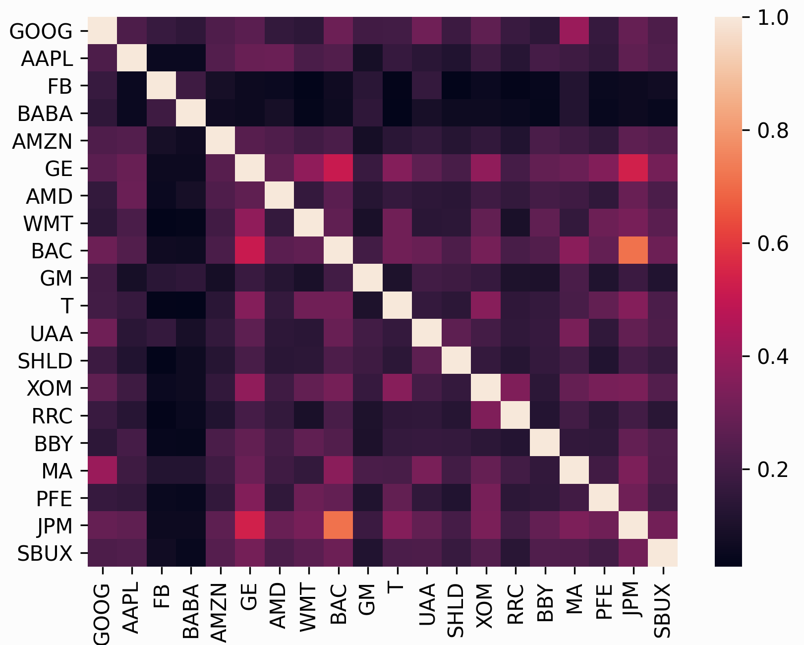](https://pyportfolioopt.readthedocs.io/en/stable/_images/corrplot.png)
In many ways, the subject of risk models is far more important than that of expected returns because historical variance is generally a much more persistent statistic than mean historical returns. In fact, research by Kritzman et al. (2010) [\[1\]](https://pyportfolioopt.readthedocs.io/en/stable/RiskModels.html#id9)
suggests that minimum variance portfolios, formed by optimising without providing expected returns, actually perform much better out of sample.
The problem, however, is that in practice we do not have access to the covariance matrix (in the same way that we don’t have access to expected returns) – the only thing we can do is to make estimates based on past data. The most straightforward approach is to just calculate the **sample covariance matrix** based on historical returns, but relatively recent (post-2000) research indicates that there are much more robust statistical estimators of the covariance matrix. In addition to providing a wrapper around the estimators in `sklearn`, PyPortfolioOpt provides some experimental alternatives such as semicovariance and exponentially weighted covariance.
Attention
Estimation of the covariance matrix is a very deep and actively-researched topic that involves statistics, econometrics, and numerical/computational approaches. PyPortfolioOpt implements several options, but there is a lot of room for more sophistication.
The `risk_models` module provides functions for estimating the covariance matrix given historical returns.
The format of the data input is the same as that in [Expected Returns](https://pyportfolioopt.readthedocs.io/en/stable/ExpectedReturns.html#expected-returns)
.
**Currently implemented:**
* fix non-positive semidefinite matrices
* general risk matrix function, allowing you to run any risk model from one function.
* sample covariance
* semicovariance
* exponentially weighted covariance
* minimum covariance determinant
* shrunk covariance matrices:
> * manual shrinkage
> * Ledoit Wolf shrinkage
> * Oracle Approximating shrinkage
* covariance to correlation matrix
Note
For any of these methods, if you would prefer to pass returns (the default is prices), set the boolean flag `returns_data=True`
`pypfopt.risk_models.``risk_matrix`(_prices_, _method='sample\_cov'_, _\*\*kwargs_)[\[source\]](https://pyportfolioopt.readthedocs.io/en/stable/_modules/pypfopt/risk_models.html#risk_matrix)
[¶](https://pyportfolioopt.readthedocs.io/en/stable/RiskModels.html#pypfopt.risk_models.risk_matrix "Permalink to this definition")
Compute a covariance matrix, using the risk model supplied in the `method` parameter.
| | |
| --- | --- |
| Parameters: | * **prices** (_pd.DataFrame_) – adjusted closing prices of the asset, each row is a date and each column is a ticker/id.
* **returns\_data** (_bool__,_ _defaults to False._) – if true, the first argument is returns instead of prices.
* **method** (_str__,_ _optional_) –
the risk model to use. Should be one of:
* `sample_cov`
* `semicovariance`
* `exp_cov`
* `ledoit_wolf`
* `ledoit_wolf_constant_variance`
* `ledoit_wolf_single_factor`
* `ledoit_wolf_constant_correlation`
* `oracle_approximating` |
| Raises: | **NotImplementedError** – if the supplied method is not recognised |
| Returns: | annualised sample covariance matrix |
| Return type: | pd.DataFrame |
`pypfopt.risk_models.``fix_nonpositive_semidefinite`(_matrix_, _fix\_method='spectral'_)[\[source\]](https://pyportfolioopt.readthedocs.io/en/stable/_modules/pypfopt/risk_models.html#fix_nonpositive_semidefinite)
[¶](https://pyportfolioopt.readthedocs.io/en/stable/RiskModels.html#pypfopt.risk_models.fix_nonpositive_semidefinite "Permalink to this definition")
Check if a covariance matrix is positive semidefinite, and if not, fix it with the chosen method.
The `spectral` method sets negative eigenvalues to zero then rebuilds the matrix, while the `diag` method adds a small positive value to the diagonal.
| | |
| --- | --- |
| Parameters: | * **matrix** (_pd.DataFrame_) – raw covariance matrix (may not be PSD)
* **fix\_method** (_str__,_ _optional_) – {“spectral”, “diag”}, defaults to “spectral” |
| Raises: | **NotImplementedError** – if a method is passed that isn’t implemented |
| Returns: | positive semidefinite covariance matrix |
| Return type: | pd.DataFrame |
Not all the calculated covariance matrices will be positive semidefinite (PSD). This method checks if a matrix is PSD and fixes it if not.
`pypfopt.risk_models.``sample_cov`(_prices_, _returns\_data=False_, _frequency=252_, _\*\*kwargs_)[\[source\]](https://pyportfolioopt.readthedocs.io/en/stable/_modules/pypfopt/risk_models.html#sample_cov)
[¶](https://pyportfolioopt.readthedocs.io/en/stable/RiskModels.html#pypfopt.risk_models.sample_cov "Permalink to this definition")
Calculate the annualised sample covariance matrix of (daily) asset returns.
| | |
| --- | --- |
| Parameters: | * **prices** (_pd.DataFrame_) – adjusted closing prices of the asset, each row is a date and each column is a ticker/id.
* **returns\_data** (_bool__,_ _defaults to False._) – if true, the first argument is returns instead of prices.
* **frequency** (_int__,_ _optional_) – number of time periods in a year, defaults to 252 (the number of trading days in a year) |
| Returns: | annualised sample covariance matrix |
| Return type: | pd.DataFrame |
This is the textbook default approach. The entries in the sample covariance matrix (which we denote as _S_) are the sample covariances between the _i_ th and _j_ th asset (the diagonals consist of variances). Although the sample covariance matrix is an unbiased estimator of the covariance matrix, i.e \\(E(S) = \\Sigma\\), in practice it suffers from misspecification error and a lack of robustness. This is particularly problematic in mean-variance optimization, because the optimizer may give extra credence to the erroneous values.
Note
This should _not_ be your default choice! Please use a shrinkage estimator instead.
`pypfopt.risk_models.``semicovariance`(_prices_, _returns\_data=False_, _benchmark=7.9e-05_, _frequency=252_, _\*\*kwargs_)[\[source\]](https://pyportfolioopt.readthedocs.io/en/stable/_modules/pypfopt/risk_models.html#semicovariance)
[¶](https://pyportfolioopt.readthedocs.io/en/stable/RiskModels.html#pypfopt.risk_models.semicovariance "Permalink to this definition")
Estimate the semicovariance matrix, i.e the covariance given that the returns are less than the benchmark.
| | |
| --- | --- |
| Parameters: | * **prices** (_pd.DataFrame_) – adjusted closing prices of the asset, each row is a date and each column is a ticker/id.
* **returns\_data** (_bool__,_ _defaults to False._) – if true, the first argument is returns instead of prices.
* **benchmark** (_float_) – the benchmark return, defaults to the daily risk-free rate, i.e \\(1.02^{(1/252)} -1\\).
* **frequency** (_int__,_ _optional_) – number of time periods in a year, defaults to 252 (the number of trading days in a year). Ensure that you use the appropriate benchmark, e.g if `frequency=12` use the monthly risk-free rate. |
| Returns: | semicovariance matrix |
| Return type: | pd.DataFrame |
The semivariance is the variance of all returns which are below some benchmark _B_ (typically the risk-free rate) – it is a common measure of downside risk. There are multiple possible ways of defining a semicovariance matrix, the main differences lying in the ‘pairwise’ nature, i.e whether we should sum over \\(\\min(r\_i,B)\\min(r\_j,B)\\) or \\(\\min(r\_ir\_j, B)\\). In this implementation, we have followed the advice of Estrada (2007) [\[2\]](https://pyportfolioopt.readthedocs.io/en/stable/RiskModels.html#id10)
, preferring:
\\\[\\frac{1}{n}\\sum\_{i = 1}^n {\\sum\_{j = 1}^n {\\min \\left( {{r\_i},B} \\right)} } \\min \\left( {{r\_j},B} \\right)\\\]
`pypfopt.risk_models.``exp_cov`(_prices_, _returns\_data=False_, _span=180_, _frequency=252_, _\*\*kwargs_)[\[source\]](https://pyportfolioopt.readthedocs.io/en/stable/_modules/pypfopt/risk_models.html#exp_cov)
[¶](https://pyportfolioopt.readthedocs.io/en/stable/RiskModels.html#pypfopt.risk_models.exp_cov "Permalink to this definition")
Estimate the exponentially-weighted covariance matrix, which gives greater weight to more recent data.
| | |
| --- | --- |
| Parameters: | * **prices** (_pd.DataFrame_) – adjusted closing prices of the asset, each row is a date and each column is a ticker/id.
* **returns\_data** (_bool__,_ _defaults to False._) – if true, the first argument is returns instead of prices.
* **span** (_int__,_ _optional_) – the span of the exponential weighting function, defaults to 180
* **frequency** (_int__,_ _optional_) – number of time periods in a year, defaults to 252 (the number of trading days in a year) |
| Returns: | annualised estimate of exponential covariance matrix |
| Return type: | pd.DataFrame |
The exponential covariance matrix is a novel way of giving more weight to recent data when calculating covariance, in the same way that the exponential moving average price is often preferred to the simple average price. For a full explanation of how this estimator works, please refer to the [blog post](https://reasonabledeviations.com/2018/08/15/exponential-covariance/)
on my academic website.
`pypfopt.risk_models.``cov_to_corr`(_cov\_matrix_)[\[source\]](https://pyportfolioopt.readthedocs.io/en/stable/_modules/pypfopt/risk_models.html#cov_to_corr)
[¶](https://pyportfolioopt.readthedocs.io/en/stable/RiskModels.html#pypfopt.risk_models.cov_to_corr "Permalink to this definition")
Convert a covariance matrix to a correlation matrix.
| | |
| --- | --- |
| Parameters: | **cov\_matrix** (_pd.DataFrame_) – covariance matrix |
| Returns: | correlation matrix |
| Return type: | pd.DataFrame |
`pypfopt.risk_models.``corr_to_cov`(_corr\_matrix_, _stdevs_)[\[source\]](https://pyportfolioopt.readthedocs.io/en/stable/_modules/pypfopt/risk_models.html#corr_to_cov)
[¶](https://pyportfolioopt.readthedocs.io/en/stable/RiskModels.html#pypfopt.risk_models.corr_to_cov "Permalink to this definition")
Convert a correlation matrix to a covariance matrix
| | |
| --- | --- |
| Parameters: | * **corr\_matrix** (_pd.DataFrame_) – correlation matrix
* **stdevs** (_array-like_) – vector of standard deviations |
| Returns: | covariance matrix |
| Return type: | pd.DataFrame |
Shrinkage estimators[¶](https://pyportfolioopt.readthedocs.io/en/stable/RiskModels.html#shrinkage-estimators "Permalink to this headline")
-------------------------------------------------------------------------------------------------------------------------------------------
A great starting point for those interested in understanding shrinkage estimators is _Honey, I Shrunk the Sample Covariance Matrix_ [\[3\]](https://pyportfolioopt.readthedocs.io/en/stable/RiskModels.html#id11)
by Ledoit and Wolf, which does a good job at capturing the intuition behind them – we will adopt the notation used therein. I have written a summary of this article, which is available on my [website](https://reasonabledeviations.com/notes/papers/ledoit_wolf_covariance/)
. A more rigorous reference can be found in Ledoit and Wolf (2001) [\[4\]](https://pyportfolioopt.readthedocs.io/en/stable/RiskModels.html#id12)
.
The essential idea is that the unbiased but often poorly estimated sample covariance can be combined with a structured estimator \\(F\\), using the below formula (where \\(\\delta\\) is the shrinkage constant):
\\\[\\hat{\\Sigma} = \\delta F + (1-\\delta) S\\\]
It is called shrinkage because it can be thought of as “shrinking” the sample covariance matrix towards the other estimator, which is accordingly called the **shrinkage target**. The shrinkage target may be significantly biased but has little estimation error. There are many possible options for the target, and each one will result in a different optimal shrinkage constant \\(\\delta\\). PyPortfolioOpt offers the following shrinkage methods:
* Ledoit-Wolf shrinkage:
> * `constant_variance` shrinkage, i.e the target is the diagonal matrix with the mean of asset variances on the diagonals and zeroes elsewhere. This is the shrinkage offered by `sklearn.LedoitWolf`.
> * `single_factor` shrinkage. Based on Sharpe’s single-index model which effectively uses a stock’s beta to the market as a risk model. See Ledoit and Wolf 2001 [\[4\]](https://pyportfolioopt.readthedocs.io/en/stable/RiskModels.html#id12)
> .
> * `constant_correlation` shrinkage, in which all pairwise correlations are set to the average correlation (sample variances are unchanged). See Ledoit and Wolf 2003 [\[3\]](https://pyportfolioopt.readthedocs.io/en/stable/RiskModels.html#id11)
>
* Oracle approximating shrinkage (OAS), invented by Chen et al. (2010) [\[5\]](https://pyportfolioopt.readthedocs.io/en/stable/RiskModels.html#id13)
, which has a lower mean-squared error than Ledoit-Wolf shrinkage when samples are Gaussian or near-Gaussian.
Tip
For most use cases, I would just go with Ledoit Wolf shrinkage, as recommended by [Quantopian](https://www.quantopian.com/)
in their lecture series on quantitative finance.
My implementations have been translated from the Matlab code on [Michael Wolf’s webpage](https://www.econ.uzh.ch/en/people/faculty/wolf/publications.html)
, with the help of [xtuanta](https://github.com/robertmartin8/PyPortfolioOpt/issues/20)
.
_class_ `pypfopt.risk_models.``CovarianceShrinkage`(_prices_, _returns\_data=False_, _frequency=252_)[\[source\]](https://pyportfolioopt.readthedocs.io/en/stable/_modules/pypfopt/risk_models.html#CovarianceShrinkage)
[¶](https://pyportfolioopt.readthedocs.io/en/stable/RiskModels.html#pypfopt.risk_models.CovarianceShrinkage "Permalink to this definition")
Provide methods for computing shrinkage estimates of the covariance matrix, using the sample covariance matrix and choosing the structured estimator to be an identity matrix multiplied by the average sample variance. The shrinkage constant can be input manually, though there exist methods (notably Ledoit Wolf) to estimate the optimal value.
Instance variables:
* `X` - pd.DataFrame (returns)
* `S` - np.ndarray (sample covariance matrix)
* `delta` - float (shrinkage constant)
* `frequency` - int
`__init__`(_prices_, _returns\_data=False_, _frequency=252_)[\[source\]](https://pyportfolioopt.readthedocs.io/en/stable/_modules/pypfopt/risk_models.html#CovarianceShrinkage.__init__)
[¶](https://pyportfolioopt.readthedocs.io/en/stable/RiskModels.html#pypfopt.risk_models.CovarianceShrinkage.__init__ "Permalink to this definition")
| | |
| --- | --- |
| Parameters: | * **prices** (_pd.DataFrame_) – adjusted closing prices of the asset, each row is a date and each column is a ticker/id.
* **returns\_data** (_bool__,_ _defaults to False._) – if true, the first argument is returns instead of prices.
* **frequency** (_int__,_ _optional_) – number of time periods in a year, defaults to 252 (the number of trading days in a year) |
`ledoit_wolf`(_shrinkage\_target='constant\_variance'_)[\[source\]](https://pyportfolioopt.readthedocs.io/en/stable/_modules/pypfopt/risk_models.html#CovarianceShrinkage.ledoit_wolf)
[¶](https://pyportfolioopt.readthedocs.io/en/stable/RiskModels.html#pypfopt.risk_models.CovarianceShrinkage.ledoit_wolf "Permalink to this definition")
Calculate the Ledoit-Wolf shrinkage estimate for a particular shrinkage target.
| | |
| --- | --- |
| Parameters: | **shrinkage\_target** (_str__,_ _optional_) – choice of shrinkage target, either `constant_variance`, `single_factor` or `constant_correlation`. Defaults to `constant_variance`. |
| Raises: | **NotImplementedError** – if the shrinkage\_target is unrecognised |
| Returns: | shrunk sample covariance matrix |
| Return type: | np.ndarray |
`oracle_approximating`()[\[source\]](https://pyportfolioopt.readthedocs.io/en/stable/_modules/pypfopt/risk_models.html#CovarianceShrinkage.oracle_approximating)
[¶](https://pyportfolioopt.readthedocs.io/en/stable/RiskModels.html#pypfopt.risk_models.CovarianceShrinkage.oracle_approximating "Permalink to this definition")
Calculate the Oracle Approximating Shrinkage estimate
| | |
| --- | --- |
| Returns: | shrunk sample covariance matrix |
| Return type: | np.ndarray |
`shrunk_covariance`(_delta=0.2_)[\[source\]](https://pyportfolioopt.readthedocs.io/en/stable/_modules/pypfopt/risk_models.html#CovarianceShrinkage.shrunk_covariance)
[¶](https://pyportfolioopt.readthedocs.io/en/stable/RiskModels.html#pypfopt.risk_models.CovarianceShrinkage.shrunk_covariance "Permalink to this definition")
Shrink a sample covariance matrix to the identity matrix (scaled by the average sample variance). This method does not estimate an optimal shrinkage parameter, it requires manual input.
| | |
| --- | --- |
| Parameters: | **delta** (_float__,_ _optional_) – shrinkage parameter, defaults to 0.2. |
| Returns: | shrunk sample covariance matrix |
| Return type: | np.ndarray |
References[¶](https://pyportfolioopt.readthedocs.io/en/stable/RiskModels.html#references "Permalink to this headline")
-----------------------------------------------------------------------------------------------------------------------
| | |
| --- | --- |
| [\[1\]](https://pyportfolioopt.readthedocs.io/en/stable/RiskModels.html#id2) | Kritzman, Page & Turkington (2010) [In defense of optimization: The fallacy of 1/N](https://www.cfapubs.org/doi/abs/10.2469/faj.v66.n2.6)
. Financial Analysts Journal, 66(2), 31-39. |
| | |
| --- | --- |
| [\[2\]](https://pyportfolioopt.readthedocs.io/en/stable/RiskModels.html#id3) | Estrada (2006), [Mean-Semivariance Optimization: A Heuristic Approach](https://papers.ssrn.com/sol3/papers.cfm?abstract_id=1028206) |
| | |
| --- | --- |
| \[3\] | _([1](https://pyportfolioopt.readthedocs.io/en/stable/RiskModels.html#id4)
, [2](https://pyportfolioopt.readthedocs.io/en/stable/RiskModels.html#id7)
)_ Ledoit, O., & Wolf, M. (2003). [Honey, I Shrunk the Sample Covariance Matrix](http://www.ledoit.net/honey.pdf)
The Journal of Portfolio Management, 30(4), 110–119. [https://doi.org/10.3905/jpm.2004.110](https://doi.org/10.3905/jpm.2004.110) |
| | |
| --- | --- |
| \[4\] | _([1](https://pyportfolioopt.readthedocs.io/en/stable/RiskModels.html#id5)
, [2](https://pyportfolioopt.readthedocs.io/en/stable/RiskModels.html#id6)
)_ Ledoit, O., & Wolf, M. (2001). [Improved estimation of the covariance matrix of stock returns with an application to portfolio selection](http://www.ledoit.net/ole2.pdf)
, 10, 603–621. |
| | |
| --- | --- |
| [\[5\]](https://pyportfolioopt.readthedocs.io/en/stable/RiskModels.html#id8) | Chen et al. (2010), [Shrinkage Algorithms for MMSE Covariance Estimation](https://arxiv.org/pdf/0907.4698.pdf)
, IEEE Transactions on Signals Processing, 58(10), 5016-5029. |
---
# Installation — PyPortfolioOpt 1.4.1 documentation
* [Docs](https://pyportfolioopt.readthedocs.io/en/stable/#)
»
* Installation
* [Edit on GitHub](https://github.com/robertmartin8/PyPortfolioOpt/blob/1db089602dee348f1eade9b981ca21cd35f1dcca/docs/index.rst)
* * *
[](https://pyportfolioopt.readthedocs.io/en/stable/_images/logo_v1-grey.png)
[](https://www.python.org/)
[](https://pypi.org/project/PyPortfolioOpt/)
[](https://opensource.org/licenses/MIT)
[](https://github.com/robertmartin8/PyPortfolioOpt/graphs/commit-activity)
PyPortfolioOpt is a library that implements portfolio optimization methods, including classical efficient frontier techniques and Black-Litterman allocation, as well as more recent developments in the field like shrinkage and Hierarchical Risk Parity, along with some novel experimental features like exponentially-weighted covariance matrices.
It is **extensive** yet easily **extensible**, and can be useful for both the casual investor and the serious practitioner. Whether you are a fundamentals-oriented investor who has identified a handful of undervalued picks, or an algorithmic trader who has a basket of strategies, PyPortfolioOpt can help you combine your alpha sources in a risk-efficient way.
Installation[¶](https://pyportfolioopt.readthedocs.io/en/stable/#installation "Permalink to this headline")
============================================================================================================
If you would like to play with PyPortfolioOpt interactively in your browser, you may launch Binder [here](https://mybinder.org/v2/gh/robertmartin8/pyportfolioopt/master/?filepath=cookbook)
. It takes a while to set up, but it lets you try out the cookbook recipes without having to install anything.
Prior to installing PyPortfolioOpt, you need to install C++. On macOS, this means that you need to install XCode Command Line Tools (see [here](https://osxdaily.com/2014/02/12/install-command-line-tools-mac-os-x/)
).
For Windows users, download Visual Studio [here](https://visualstudio.microsoft.com/thank-you-downloading-visual-studio/?sku=BuildTools&rel=16)
, with additional instructions [here](https://drive.google.com/file/d/0B4GsMXCRaSSIOWpYQkstajlYZ0tPVkNQSElmTWh1dXFaYkJr/view)
.
Installation can then be done via pip:
pip install PyPortfolioOpt
For the sake of best practice, it is good to do this with a dependency manager. I suggest you set yourself up with [poetry](https://github.com/sdispater/poetry)
, then within a new poetry project run:
poetry add PyPortfolioOpt
The alternative is to clone/download the project, then in the project directory run
python setup.py install
Thanks to Thomas Schmelzer, PyPortfolioOpt now supports Docker (requires **make**, **docker**, **docker-compose**). Build your first container with `make build`; run tests with `make test`. For more information, please read [this guide](https://docker-curriculum.com/#introduction)
.
Note
If any of these methods don’t work, please [raise an issue](https://github.com/robertmartin8/PyPortfolioOpt/issues)
with the ‘packaging’ label on GitHub
For developers[¶](https://pyportfolioopt.readthedocs.io/en/stable/#for-developers "Permalink to this headline")
----------------------------------------------------------------------------------------------------------------
If you are planning on using PyPortfolioOpt as a starting template for significant modifications, it probably makes sense to clone the repository and to just use the source code
git clone https://github.com/robertmartin8/PyPortfolioOpt
Alternatively, if you still want the convenience of a global `from pypfopt import x`, you should try
pip install -e git+https://github.com/robertmartin8/PyPortfolioOpt.git
A Quick Example[¶](https://pyportfolioopt.readthedocs.io/en/stable/#a-quick-example "Permalink to this headline")
==================================================================================================================
This section contains a quick look at what PyPortfolioOpt can do. For a guided tour, please check out the [User Guide](https://pyportfolioopt.readthedocs.io/en/stable/UserGuide.html#user-guide)
. For even more examples, check out the Jupyter notebooks in the [cookbook](https://github.com/robertmartin8/PyPortfolioOpt/tree/master/cookbook)
.
If you already have expected returns `mu` and a risk model `S` for your set of assets, generating an optimal portfolio is as easy as:
from pypfopt.efficient\_frontier import EfficientFrontier
ef \= EfficientFrontier(mu, S)
weights \= ef.max\_sharpe()
However, if you would like to use PyPortfolioOpt’s built-in methods for calculating the expected returns and covariance matrix from historical data, that’s fine too:
import pandas as pd
from pypfopt.efficient\_frontier import EfficientFrontier
from pypfopt import risk\_models
from pypfopt import expected\_returns
\# Read in price data
df \= pd.read\_csv("tests/resources/stock\_prices.csv", parse\_dates\=True, index\_col\="date")
\# Calculate expected returns and sample covariance
mu \= expected\_returns.mean\_historical\_return(df)
S \= risk\_models.sample\_cov(df)
\# Optimize for maximal Sharpe ratio
ef \= EfficientFrontier(mu, S)
weights \= ef.max\_sharpe()
ef.portfolio\_performance(verbose\=True)
This outputs the following:
Expected annual return: 33.0%
Annual volatility: 21.7%
Sharpe Ratio: 1.43
Contents[¶](https://pyportfolioopt.readthedocs.io/en/stable/#contents "Permalink to this headline")
====================================================================================================
* [User Guide](https://pyportfolioopt.readthedocs.io/en/stable/UserGuide.html)
* [Processing historical prices](https://pyportfolioopt.readthedocs.io/en/stable/UserGuide.html#processing-historical-prices)
* [Mean-variance optimization](https://pyportfolioopt.readthedocs.io/en/stable/UserGuide.html#mean-variance-optimization)
* [Improving performance](https://pyportfolioopt.readthedocs.io/en/stable/UserGuide.html#improving-performance)
* [References](https://pyportfolioopt.readthedocs.io/en/stable/UserGuide.html#references)
* [Expected Returns](https://pyportfolioopt.readthedocs.io/en/stable/ExpectedReturns.html)
* [Risk Models](https://pyportfolioopt.readthedocs.io/en/stable/RiskModels.html)
* [Shrinkage estimators](https://pyportfolioopt.readthedocs.io/en/stable/RiskModels.html#shrinkage-estimators)
* [References](https://pyportfolioopt.readthedocs.io/en/stable/RiskModels.html#references)
* [Mean-Variance Optimization](https://pyportfolioopt.readthedocs.io/en/stable/MeanVariance.html)
* [Structure](https://pyportfolioopt.readthedocs.io/en/stable/MeanVariance.html#structure)
* [Basic Usage](https://pyportfolioopt.readthedocs.io/en/stable/MeanVariance.html#module-pypfopt.efficient_frontier)
* [Adding objectives and constraints](https://pyportfolioopt.readthedocs.io/en/stable/MeanVariance.html#adding-objectives-and-constraints)
* [Objective functions](https://pyportfolioopt.readthedocs.io/en/stable/MeanVariance.html#module-pypfopt.objective_functions)
* [More on L2 Regularisation](https://pyportfolioopt.readthedocs.io/en/stable/MeanVariance.html#more-on-l2-regularisation)
* [References](https://pyportfolioopt.readthedocs.io/en/stable/MeanVariance.html#references)
* [General Efficient Frontier](https://pyportfolioopt.readthedocs.io/en/stable/GeneralEfficientFrontier.html)
* [Efficient Semivariance](https://pyportfolioopt.readthedocs.io/en/stable/GeneralEfficientFrontier.html#efficient-semivariance)
* [Efficient CVaR](https://pyportfolioopt.readthedocs.io/en/stable/GeneralEfficientFrontier.html#efficient-cvar)
* [Custom optimization problems](https://pyportfolioopt.readthedocs.io/en/stable/GeneralEfficientFrontier.html#custom-optimization-problems)
* [References](https://pyportfolioopt.readthedocs.io/en/stable/GeneralEfficientFrontier.html#references)
* [Black-Litterman Allocation](https://pyportfolioopt.readthedocs.io/en/stable/BlackLitterman.html)
* [Priors](https://pyportfolioopt.readthedocs.io/en/stable/BlackLitterman.html#priors)
* [Views](https://pyportfolioopt.readthedocs.io/en/stable/BlackLitterman.html#views)
* [Confidence matrix and tau](https://pyportfolioopt.readthedocs.io/en/stable/BlackLitterman.html#confidence-matrix-and-tau)
* [Output of the BL model](https://pyportfolioopt.readthedocs.io/en/stable/BlackLitterman.html#output-of-the-bl-model)
* [Documentation reference](https://pyportfolioopt.readthedocs.io/en/stable/BlackLitterman.html#module-pypfopt.black_litterman)
* [References](https://pyportfolioopt.readthedocs.io/en/stable/BlackLitterman.html#references)
* [Other Optimizers](https://pyportfolioopt.readthedocs.io/en/stable/OtherOptimizers.html)
* [Hierarchical Risk Parity (HRP)](https://pyportfolioopt.readthedocs.io/en/stable/OtherOptimizers.html#hierarchical-risk-parity-hrp)
* [The Critical Line Algorithm](https://pyportfolioopt.readthedocs.io/en/stable/OtherOptimizers.html#the-critical-line-algorithm)
* [Implementing your own optimizer](https://pyportfolioopt.readthedocs.io/en/stable/OtherOptimizers.html#implementing-your-own-optimizer)
* [References](https://pyportfolioopt.readthedocs.io/en/stable/OtherOptimizers.html#references)
* [Post-processing weights](https://pyportfolioopt.readthedocs.io/en/stable/Postprocessing.html)
* [Greedy algorithm](https://pyportfolioopt.readthedocs.io/en/stable/Postprocessing.html#greedy-algorithm)
* [Integer programming](https://pyportfolioopt.readthedocs.io/en/stable/Postprocessing.html#integer-programming)
* [Dealing with shorts](https://pyportfolioopt.readthedocs.io/en/stable/Postprocessing.html#dealing-with-shorts)
* [Documentation reference](https://pyportfolioopt.readthedocs.io/en/stable/Postprocessing.html#module-pypfopt.discrete_allocation)
* [Plotting](https://pyportfolioopt.readthedocs.io/en/stable/Plotting.html)
* [Documentation reference](https://pyportfolioopt.readthedocs.io/en/stable/Plotting.html#module-pypfopt.plotting)
Other information
* [FAQs](https://pyportfolioopt.readthedocs.io/en/stable/FAQ.html)
* [Roadmap and Changelog](https://pyportfolioopt.readthedocs.io/en/stable/Roadmap.html)
* [Contributing](https://pyportfolioopt.readthedocs.io/en/stable/Contributing.html)
* [About](https://pyportfolioopt.readthedocs.io/en/stable/About.html)
Project principles and design decisions[¶](https://pyportfolioopt.readthedocs.io/en/stable/#project-principles-and-design-decisions "Permalink to this headline")
==================================================================================================================================================================
* It should be easy to swap out individual components of the optimization process with the user’s proprietary improvements.
* Usability is everything: it is better to be self-explanatory than consistent.
* There is no point in portfolio optimization unless it can be practically applied to real asset prices.
* Everything that has been implemented should be tested.
* Inline documentation is good: dedicated (separate) documentation is better. The two are not mutually exclusive.
* Formatting should never get in the way of good code: because of this, I have deferred **all** formatting decisions to [Black](https://github.com/ambv/black)
.
Advantages over existing implementations[¶](https://pyportfolioopt.readthedocs.io/en/stable/#advantages-over-existing-implementations "Permalink to this headline")
====================================================================================================================================================================
* Includes both classical methods (Markowitz 1952 and Black-Litterman), suggested best practices (e.g covariance shrinkage), along with many recent developments and novel features, like L2 regularisation, exponential covariance, hierarchical risk parity.
* Native support for pandas dataframes: easily input your daily prices data.
* Extensive practical tests, which use real-life data.
* Easy to combine with your proprietary strategies and models.
* Robust to missing data, and price-series of different lengths (e.g FB data only goes back to 2012 whereas AAPL data goes back to 1980).
Contributors[¶](https://pyportfolioopt.readthedocs.io/en/stable/#contributors "Permalink to this headline")
============================================================================================================
This is a non-exhaustive unordered list of contributors. I am sincerely grateful for all of your efforts!
* Philipp Schiele
* Carl Peasnell
* Felipe Schneider
* Dingyuan Wang
* Pat Newell
* Aditya Bhutra
* Thomas Schmelzer
* Rich Caputo
* Nicolas Knudde
Indices and tables[¶](https://pyportfolioopt.readthedocs.io/en/stable/#indices-and-tables "Permalink to this headline")
========================================================================================================================
* [Index](https://pyportfolioopt.readthedocs.io/en/stable/genindex.html)
* [Module Index](https://pyportfolioopt.readthedocs.io/en/stable/py-modindex.html)
* [Search Page](https://pyportfolioopt.readthedocs.io/en/stable/search.html)
---
# Risk Models — PyPortfolioOpt 1.5.4 documentation
* [Docs](https://pyportfolioopt.readthedocs.io/en/latest/index.html)
»
* Risk Models
* [Edit on GitHub](https://github.com/robertmartin8/PyPortfolioOpt/blob/master/docs/RiskModels.rst)
* * *
Risk Models[¶](https://pyportfolioopt.readthedocs.io/en/latest/RiskModels.html#risk-models "Permalink to this headline")
=========================================================================================================================
In addition to the expected returns, mean-variance optimization requires a **risk model**, some way of quantifying asset risk. The most commonly-used risk model is the covariance matrix, which describes asset volatilities and their co-dependence. This is important because one of the principles of diversification is that risk can be reduced by making many uncorrelated bets (correlation is just normalised covariance).
[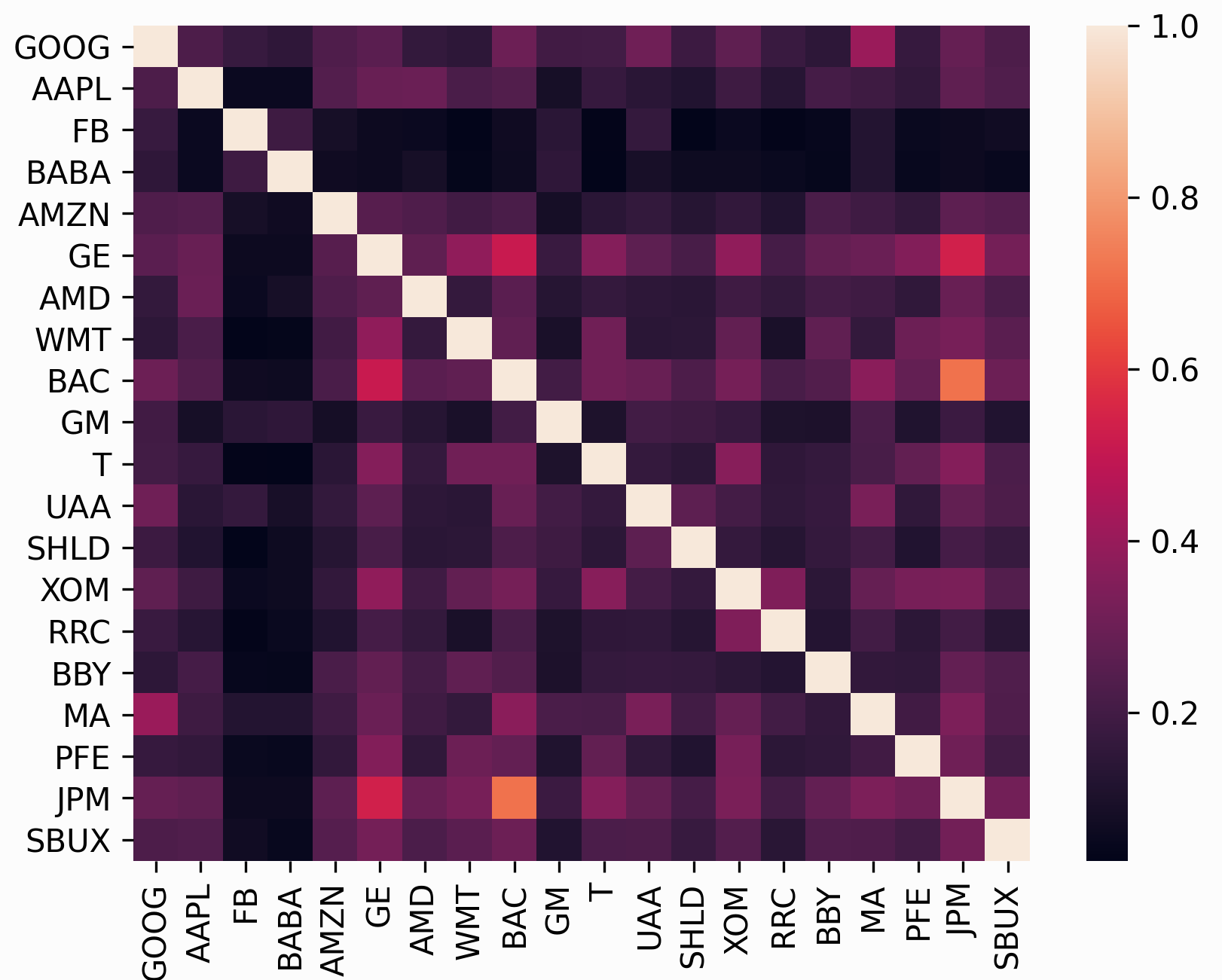](https://pyportfolioopt.readthedocs.io/en/latest/_images/corrplot.png)
In many ways, the subject of risk models is far more important than that of expected returns because historical variance is generally a much more persistent statistic than mean historical returns. In fact, research by Kritzman et al. (2010) [\[1\]](https://pyportfolioopt.readthedocs.io/en/latest/RiskModels.html#id9)
suggests that minimum variance portfolios, formed by optimising without providing expected returns, actually perform much better out of sample.
The problem, however, is that in practice we do not have access to the covariance matrix (in the same way that we don’t have access to expected returns) – the only thing we can do is to make estimates based on past data. The most straightforward approach is to just calculate the **sample covariance matrix** based on historical returns, but relatively recent (post-2000) research indicates that there are much more robust statistical estimators of the covariance matrix. In addition to providing a wrapper around the estimators in `sklearn`, PyPortfolioOpt provides some experimental alternatives such as semicovariance and exponentially weighted covariance.
Attention
Estimation of the covariance matrix is a very deep and actively-researched topic that involves statistics, econometrics, and numerical/computational approaches. PyPortfolioOpt implements several options, but there is a lot of room for more sophistication.
The `risk_models` module provides functions for estimating the covariance matrix given historical returns.
The format of the data input is the same as that in [Expected Returns](https://pyportfolioopt.readthedocs.io/en/latest/ExpectedReturns.html#expected-returns)
.
**Currently implemented:**
* fix non-positive semidefinite matrices
* general risk matrix function, allowing you to run any risk model from one function.
* sample covariance
* semicovariance
* exponentially weighted covariance
* minimum covariance determinant
* shrunk covariance matrices:
> * manual shrinkage
> * Ledoit Wolf shrinkage
> * Oracle Approximating shrinkage
* covariance to correlation matrix
Note
For any of these methods, if you would prefer to pass returns (the default is prices), set the boolean flag `returns_data=True`
`pypfopt.risk_models.``risk_matrix`(_prices_, _method='sample\_cov'_, _\*\*kwargs_)[\[source\]](https://pyportfolioopt.readthedocs.io/en/latest/_modules/pypfopt/risk_models.html#risk_matrix)
[¶](https://pyportfolioopt.readthedocs.io/en/latest/RiskModels.html#pypfopt.risk_models.risk_matrix "Permalink to this definition")
Compute a covariance matrix, using the risk model supplied in the `method` parameter.
| | |
| --- | --- |
| Parameters: | * **prices** (_pd.DataFrame_) – adjusted closing prices of the asset, each row is a date and each column is a ticker/id.
* **returns\_data** (_bool__,_ _defaults to False._) – if true, the first argument is returns instead of prices.
* **method** (_str__,_ _optional_) –
the risk model to use. Should be one of:
* `sample_cov`
* `semicovariance`
* `exp_cov`
* `ledoit_wolf`
* `ledoit_wolf_constant_variance`
* `ledoit_wolf_single_factor`
* `ledoit_wolf_constant_correlation`
* `oracle_approximating` |
| Raises: | **NotImplementedError** – if the supplied method is not recognised |
| Returns: | annualised sample covariance matrix |
| Return type: | pd.DataFrame |
`pypfopt.risk_models.``fix_nonpositive_semidefinite`(_matrix_, _fix\_method='spectral'_)[\[source\]](https://pyportfolioopt.readthedocs.io/en/latest/_modules/pypfopt/risk_models.html#fix_nonpositive_semidefinite)
[¶](https://pyportfolioopt.readthedocs.io/en/latest/RiskModels.html#pypfopt.risk_models.fix_nonpositive_semidefinite "Permalink to this definition")
Check if a covariance matrix is positive semidefinite, and if not, fix it with the chosen method.
The `spectral` method sets negative eigenvalues to zero then rebuilds the matrix, while the `diag` method adds a small positive value to the diagonal.
| | |
| --- | --- |
| Parameters: | * **matrix** (_pd.DataFrame_) – raw covariance matrix (may not be PSD)
* **fix\_method** (_str__,_ _optional_) – {“spectral”, “diag”}, defaults to “spectral” |
| Raises: | **NotImplementedError** – if a method is passed that isn’t implemented |
| Returns: | positive semidefinite covariance matrix |
| Return type: | pd.DataFrame |
Not all the calculated covariance matrices will be positive semidefinite (PSD). This method checks if a matrix is PSD and fixes it if not.
`pypfopt.risk_models.``sample_cov`(_prices_, _returns\_data=False_, _frequency=252_, _log\_returns=False_, _\*\*kwargs_)[\[source\]](https://pyportfolioopt.readthedocs.io/en/latest/_modules/pypfopt/risk_models.html#sample_cov)
[¶](https://pyportfolioopt.readthedocs.io/en/latest/RiskModels.html#pypfopt.risk_models.sample_cov "Permalink to this definition")
Calculate the annualised sample covariance matrix of (daily) asset returns.
| | |
| --- | --- |
| Parameters: | * **prices** (_pd.DataFrame_) – adjusted closing prices of the asset, each row is a date and each column is a ticker/id.
* **returns\_data** (_bool__,_ _defaults to False._) – if true, the first argument is returns instead of prices.
* **frequency** (_int__,_ _optional_) – number of time periods in a year, defaults to 252 (the number of trading days in a year)
* **log\_returns** (_bool__,_ _defaults to False_) – whether to compute using log returns |
| Returns: | annualised sample covariance matrix |
| Return type: | pd.DataFrame |
This is the textbook default approach. The entries in the sample covariance matrix (which we denote as _S_) are the sample covariances between the _i_ th and _j_ th asset (the diagonals consist of variances). Although the sample covariance matrix is an unbiased estimator of the covariance matrix, i.e \\(E(S) = \\Sigma\\), in practice it suffers from misspecification error and a lack of robustness. This is particularly problematic in mean-variance optimization, because the optimizer may give extra credence to the erroneous values.
Note
This should _not_ be your default choice! Please use a shrinkage estimator instead.
`pypfopt.risk_models.``semicovariance`(_prices_, _returns\_data=False_, _benchmark=7.9e-05_, _frequency=252_, _log\_returns=False_, _\*\*kwargs_)[\[source\]](https://pyportfolioopt.readthedocs.io/en/latest/_modules/pypfopt/risk_models.html#semicovariance)
[¶](https://pyportfolioopt.readthedocs.io/en/latest/RiskModels.html#pypfopt.risk_models.semicovariance "Permalink to this definition")
Estimate the semicovariance matrix, i.e the covariance given that the returns are less than the benchmark.
| | |
| --- | --- |
| Parameters: | * **prices** (_pd.DataFrame_) – adjusted closing prices of the asset, each row is a date and each column is a ticker/id.
* **returns\_data** (_bool__,_ _defaults to False._) – if true, the first argument is returns instead of prices.
* **benchmark** (_float_) – the benchmark return, defaults to the daily risk-free rate, i.e \\(1.02^{(1/252)} -1\\).
* **frequency** (_int__,_ _optional_) – number of time periods in a year, defaults to 252 (the number of trading days in a year). Ensure that you use the appropriate benchmark, e.g if `frequency=12` use the monthly risk-free rate.
* **log\_returns** (_bool__,_ _defaults to False_) – whether to compute using log returns |
| Returns: | semicovariance matrix |
| Return type: | pd.DataFrame |
The semivariance is the variance of all returns which are below some benchmark _B_ (typically the risk-free rate) – it is a common measure of downside risk. There are multiple possible ways of defining a semicovariance matrix, the main differences lying in the ‘pairwise’ nature, i.e whether we should sum over \\(\\min(r\_i,B)\\min(r\_j,B)\\) or \\(\\min(r\_ir\_j, B)\\). In this implementation, we have followed the advice of Estrada (2007) [\[2\]](https://pyportfolioopt.readthedocs.io/en/latest/RiskModels.html#id10)
, preferring:
\\\[\\frac{1}{n}\\sum\_{i = 1}^n {\\sum\_{j = 1}^n {\\min \\left( {{r\_i},B} \\right)} } \\min \\left( {{r\_j},B} \\right)\\\]
`pypfopt.risk_models.``exp_cov`(_prices_, _returns\_data=False_, _span=180_, _frequency=252_, _log\_returns=False_, _\*\*kwargs_)[\[source\]](https://pyportfolioopt.readthedocs.io/en/latest/_modules/pypfopt/risk_models.html#exp_cov)
[¶](https://pyportfolioopt.readthedocs.io/en/latest/RiskModels.html#pypfopt.risk_models.exp_cov "Permalink to this definition")
Estimate the exponentially-weighted covariance matrix, which gives greater weight to more recent data.
| | |
| --- | --- |
| Parameters: | * **prices** (_pd.DataFrame_) – adjusted closing prices of the asset, each row is a date and each column is a ticker/id.
* **returns\_data** (_bool__,_ _defaults to False._) – if true, the first argument is returns instead of prices.
* **span** (_int__,_ _optional_) – the span of the exponential weighting function, defaults to 180
* **frequency** (_int__,_ _optional_) – number of time periods in a year, defaults to 252 (the number of trading days in a year)
* **log\_returns** (_bool__,_ _defaults to False_) – whether to compute using log returns |
| Returns: | annualised estimate of exponential covariance matrix |
| Return type: | pd.DataFrame |
The exponential covariance matrix is a novel way of giving more weight to recent data when calculating covariance, in the same way that the exponential moving average price is often preferred to the simple average price. For a full explanation of how this estimator works, please refer to the [blog post](https://reasonabledeviations.com/2018/08/15/exponential-covariance/)
on my academic website.
`pypfopt.risk_models.``cov_to_corr`(_cov\_matrix_)[\[source\]](https://pyportfolioopt.readthedocs.io/en/latest/_modules/pypfopt/risk_models.html#cov_to_corr)
[¶](https://pyportfolioopt.readthedocs.io/en/latest/RiskModels.html#pypfopt.risk_models.cov_to_corr "Permalink to this definition")
Convert a covariance matrix to a correlation matrix.
| | |
| --- | --- |
| Parameters: | **cov\_matrix** (_pd.DataFrame_) – covariance matrix |
| Returns: | correlation matrix |
| Return type: | pd.DataFrame |
`pypfopt.risk_models.``corr_to_cov`(_corr\_matrix_, _stdevs_)[\[source\]](https://pyportfolioopt.readthedocs.io/en/latest/_modules/pypfopt/risk_models.html#corr_to_cov)
[¶](https://pyportfolioopt.readthedocs.io/en/latest/RiskModels.html#pypfopt.risk_models.corr_to_cov "Permalink to this definition")
Convert a correlation matrix to a covariance matrix
| | |
| --- | --- |
| Parameters: | * **corr\_matrix** (_pd.DataFrame_) – correlation matrix
* **stdevs** (_array-like_) – vector of standard deviations |
| Returns: | covariance matrix |
| Return type: | pd.DataFrame |
Shrinkage estimators[¶](https://pyportfolioopt.readthedocs.io/en/latest/RiskModels.html#shrinkage-estimators "Permalink to this headline")
-------------------------------------------------------------------------------------------------------------------------------------------
A great starting point for those interested in understanding shrinkage estimators is _Honey, I Shrunk the Sample Covariance Matrix_ [\[3\]](https://pyportfolioopt.readthedocs.io/en/latest/RiskModels.html#id11)
by Ledoit and Wolf, which does a good job at capturing the intuition behind them – we will adopt the notation used therein. I have written a summary of this article, which is available on my [website](https://reasonabledeviations.com/notes/papers/ledoit_wolf_covariance/)
. A more rigorous reference can be found in Ledoit and Wolf (2001) [\[4\]](https://pyportfolioopt.readthedocs.io/en/latest/RiskModels.html#id12)
.
The essential idea is that the unbiased but often poorly estimated sample covariance can be combined with a structured estimator \\(F\\), using the below formula (where \\(\\delta\\) is the shrinkage constant):
\\\[\\hat{\\Sigma} = \\delta F + (1-\\delta) S\\\]
It is called shrinkage because it can be thought of as “shrinking” the sample covariance matrix towards the other estimator, which is accordingly called the **shrinkage target**. The shrinkage target may be significantly biased but has little estimation error. There are many possible options for the target, and each one will result in a different optimal shrinkage constant \\(\\delta\\). PyPortfolioOpt offers the following shrinkage methods:
* Ledoit-Wolf shrinkage:
> * `constant_variance` shrinkage, i.e the target is the diagonal matrix with the mean of asset variances on the diagonals and zeroes elsewhere. This is the shrinkage offered by `sklearn.LedoitWolf`.
> * `single_factor` shrinkage. Based on Sharpe’s single-index model which effectively uses a stock’s beta to the market as a risk model. See Ledoit and Wolf 2001 [\[4\]](https://pyportfolioopt.readthedocs.io/en/latest/RiskModels.html#id12)
> .
> * `constant_correlation` shrinkage, in which all pairwise correlations are set to the average correlation (sample variances are unchanged). See Ledoit and Wolf 2003 [\[3\]](https://pyportfolioopt.readthedocs.io/en/latest/RiskModels.html#id11)
>
* Oracle approximating shrinkage (OAS), invented by Chen et al. (2010) [\[5\]](https://pyportfolioopt.readthedocs.io/en/latest/RiskModels.html#id13)
, which has a lower mean-squared error than Ledoit-Wolf shrinkage when samples are Gaussian or near-Gaussian.
Tip
For most use cases, I would just go with Ledoit Wolf shrinkage, as recommended by [Quantopian](https://www.quantopian.com/)
in their lecture series on quantitative finance.
My implementations have been translated from the Matlab code on [Michael Wolf’s webpage](https://www.econ.uzh.ch/en/people/faculty/wolf/publications.html)
, with the help of [xtuanta](https://github.com/robertmartin8/PyPortfolioOpt/issues/20)
.
_class_ `pypfopt.risk_models.``CovarianceShrinkage`(_prices_, _returns\_data=False_, _frequency=252_, _log\_returns=False_)[\[source\]](https://pyportfolioopt.readthedocs.io/en/latest/_modules/pypfopt/risk_models.html#CovarianceShrinkage)
[¶](https://pyportfolioopt.readthedocs.io/en/latest/RiskModels.html#pypfopt.risk_models.CovarianceShrinkage "Permalink to this definition")
Provide methods for computing shrinkage estimates of the covariance matrix, using the sample covariance matrix and choosing the structured estimator to be an identity matrix multiplied by the average sample variance. The shrinkage constant can be input manually, though there exist methods (notably Ledoit Wolf) to estimate the optimal value.
Instance variables:
* `X` - pd.DataFrame (returns)
* `S` - np.ndarray (sample covariance matrix)
* `delta` - float (shrinkage constant)
* `frequency` - int
`__init__`(_prices_, _returns\_data=False_, _frequency=252_, _log\_returns=False_)[\[source\]](https://pyportfolioopt.readthedocs.io/en/latest/_modules/pypfopt/risk_models.html#CovarianceShrinkage.__init__)
[¶](https://pyportfolioopt.readthedocs.io/en/latest/RiskModels.html#pypfopt.risk_models.CovarianceShrinkage.__init__ "Permalink to this definition")
| | |
| --- | --- |
| Parameters: | * **prices** (_pd.DataFrame_) – adjusted closing prices of the asset, each row is a date and each column is a ticker/id.
* **returns\_data** (_bool__,_ _defaults to False._) – if true, the first argument is returns instead of prices.
* **frequency** (_int__,_ _optional_) – number of time periods in a year, defaults to 252 (the number of trading days in a year)
* **log\_returns** (_bool__,_ _defaults to False_) – whether to compute using log returns |
`ledoit_wolf`(_shrinkage\_target='constant\_variance'_)[\[source\]](https://pyportfolioopt.readthedocs.io/en/latest/_modules/pypfopt/risk_models.html#CovarianceShrinkage.ledoit_wolf)
[¶](https://pyportfolioopt.readthedocs.io/en/latest/RiskModels.html#pypfopt.risk_models.CovarianceShrinkage.ledoit_wolf "Permalink to this definition")
Calculate the Ledoit-Wolf shrinkage estimate for a particular shrinkage target.
| | |
| --- | --- |
| Parameters: | **shrinkage\_target** (_str__,_ _optional_) – choice of shrinkage target, either `constant_variance`, `single_factor` or `constant_correlation`. Defaults to `constant_variance`. |
| Raises: | **NotImplementedError** – if the shrinkage\_target is unrecognised |
| Returns: | shrunk sample covariance matrix |
| Return type: | np.ndarray |
`oracle_approximating`()[\[source\]](https://pyportfolioopt.readthedocs.io/en/latest/_modules/pypfopt/risk_models.html#CovarianceShrinkage.oracle_approximating)
[¶](https://pyportfolioopt.readthedocs.io/en/latest/RiskModels.html#pypfopt.risk_models.CovarianceShrinkage.oracle_approximating "Permalink to this definition")
Calculate the Oracle Approximating Shrinkage estimate
| | |
| --- | --- |
| Returns: | shrunk sample covariance matrix |
| Return type: | np.ndarray |
`shrunk_covariance`(_delta=0.2_)[\[source\]](https://pyportfolioopt.readthedocs.io/en/latest/_modules/pypfopt/risk_models.html#CovarianceShrinkage.shrunk_covariance)
[¶](https://pyportfolioopt.readthedocs.io/en/latest/RiskModels.html#pypfopt.risk_models.CovarianceShrinkage.shrunk_covariance "Permalink to this definition")
Shrink a sample covariance matrix to the identity matrix (scaled by the average sample variance). This method does not estimate an optimal shrinkage parameter, it requires manual input.
| | |
| --- | --- |
| Parameters: | **delta** (_float__,_ _optional_) – shrinkage parameter, defaults to 0.2. |
| Returns: | shrunk sample covariance matrix |
| Return type: | np.ndarray |
References[¶](https://pyportfolioopt.readthedocs.io/en/latest/RiskModels.html#references "Permalink to this headline")
-----------------------------------------------------------------------------------------------------------------------
| | |
| --- | --- |
| [\[1\]](https://pyportfolioopt.readthedocs.io/en/latest/RiskModels.html#id2) | Kritzman, Page & Turkington (2010) [In defense of optimization: The fallacy of 1/N](https://www.cfapubs.org/doi/abs/10.2469/faj.v66.n2.6)
. Financial Analysts Journal, 66(2), 31-39. |
| | |
| --- | --- |
| [\[2\]](https://pyportfolioopt.readthedocs.io/en/latest/RiskModels.html#id3) | Estrada (2006), [Mean-Semivariance Optimization: A Heuristic Approach](https://papers.ssrn.com/sol3/papers.cfm?abstract_id=1028206) |
| | |
| --- | --- |
| \[3\] | _([1](https://pyportfolioopt.readthedocs.io/en/latest/RiskModels.html#id4)
, [2](https://pyportfolioopt.readthedocs.io/en/latest/RiskModels.html#id7)
)_ Ledoit, O., & Wolf, M. (2003). [Honey, I Shrunk the Sample Covariance Matrix](http://www.ledoit.net/honey.pdf)
The Journal of Portfolio Management, 30(4), 110–119. [https://doi.org/10.3905/jpm.2004.110](https://doi.org/10.3905/jpm.2004.110) |
| | |
| --- | --- |
| \[4\] | _([1](https://pyportfolioopt.readthedocs.io/en/latest/RiskModels.html#id5)
, [2](https://pyportfolioopt.readthedocs.io/en/latest/RiskModels.html#id6)
)_ Ledoit, O., & Wolf, M. (2001). [Improved estimation of the covariance matrix of stock returns with an application to portfolio selection](http://www.ledoit.net/ole2.pdf)
, 10, 603–621. |
| | |
| --- | --- |
| [\[5\]](https://pyportfolioopt.readthedocs.io/en/latest/RiskModels.html#id8) | Chen et al. (2010), [Shrinkage Algorithms for MMSE Covariance Estimation](https://arxiv.org/pdf/0907.4698.pdf)
, IEEE Transactions on Signals Processing, 58(10), 5016-5029. |
---
# Installation — PyPortfolioOpt 1.5.4 documentation
* [Docs](https://pyportfolioopt.readthedocs.io/en/latest/#)
»
* Installation
* [Edit on GitHub](https://github.com/robertmartin8/PyPortfolioOpt/blob/master/docs/index.rst)
* * *
[](https://pyportfolioopt.readthedocs.io/en/latest/_images/logo_v1-grey.png)
[](https://www.python.org/)
[](https://pypi.org/project/PyPortfolioOpt/)
[](https://opensource.org/licenses/MIT)
[](https://github.com/robertmartin8/PyPortfolioOpt/graphs/commit-activity)
[](https://doi.org/10.21105/joss.03066)
PyPortfolioOpt is a library that implements portfolio optimization methods, including classical efficient frontier techniques and Black-Litterman allocation, as well as more recent developments in the field like shrinkage and Hierarchical Risk Parity, along with some novel experimental features like exponentially-weighted covariance matrices.
It is **extensive** yet easily **extensible**, and can be useful for both the casual investor and the serious practitioner. Whether you are a fundamentals-oriented investor who has identified a handful of undervalued picks, or an algorithmic trader who has a basket of strategies, PyPortfolioOpt can help you combine your alpha sources in a risk-efficient way.
Installation[¶](https://pyportfolioopt.readthedocs.io/en/latest/#installation "Permalink to this headline")
============================================================================================================
If you would like to play with PyPortfolioOpt interactively in your browser, you may launch Binder [here](https://mybinder.org/v2/gh/robertmartin8/pyportfolioopt/master/?filepath=cookbook)
. It takes a while to set up, but it lets you try out the cookbook recipes without having to install anything.
Prior to installing PyPortfolioOpt, you need to install C++. On macOS, this means that you need to install XCode Command Line Tools (see [here](https://osxdaily.com/2014/02/12/install-command-line-tools-mac-os-x/)
).
For Windows users, download Visual Studio [here](https://visualstudio.microsoft.com/thank-you-downloading-visual-studio/?sku=BuildTools&rel=16)
, with additional instructions [here](https://docs.google.com/presentation/d/0B4GsMXCRaSSIOWpYQkstajlYZ0tPVkNQSElmTWh1dXFaYkJr/edit?usp=sharing&ouid=117107708911390632479&resourcekey=0-HEezB2NFstz1GjKDkroJSQ&rtpof=true&sd=true)
.
Installation can then be done via pip:
pip install PyPortfolioOpt
(you may need to follow separate installation instructions for [cvxopt](https://cvxopt.org/install/index.html#)
and [cvxpy](https://www.cvxpy.org/install/)
).
For the sake of best practice, it is good to do this with a dependency manager. I suggest you set yourself up with [poetry](https://github.com/sdispater/poetry)
, then within a new poetry project run:
poetry add PyPortfolioOpt
The alternative is to clone/download the project, then in the project directory run
python setup.py install
Thanks to Thomas Schmelzer, PyPortfolioOpt now supports Docker (requires **make**, **docker**, **docker-compose**). Build your first container with `make build`; run tests with `make test`. For more information, please read [this guide](https://docker-curriculum.com/#introduction)
.
Note
If any of these methods don’t work, please [raise an issue](https://github.com/robertmartin8/PyPortfolioOpt/issues)
with the ‘packaging’ label on GitHub
For developers[¶](https://pyportfolioopt.readthedocs.io/en/latest/#for-developers "Permalink to this headline")
----------------------------------------------------------------------------------------------------------------
If you are planning on using PyPortfolioOpt as a starting template for significant modifications, it probably makes sense to clone the repository and to just use the source code
git clone https://github.com/robertmartin8/PyPortfolioOpt
Alternatively, if you still want the convenience of a global `from pypfopt import x`, you should try
pip install -e git+https://github.com/robertmartin8/PyPortfolioOpt.git
A Quick Example[¶](https://pyportfolioopt.readthedocs.io/en/latest/#a-quick-example "Permalink to this headline")
==================================================================================================================
This section contains a quick look at what PyPortfolioOpt can do. For a guided tour, please check out the [User Guide](https://pyportfolioopt.readthedocs.io/en/latest/UserGuide.html#user-guide)
. For even more examples, check out the Jupyter notebooks in the [cookbook](https://github.com/robertmartin8/PyPortfolioOpt/tree/master/cookbook)
.
If you already have expected returns `mu` and a risk model `S` for your set of assets, generating an optimal portfolio is as easy as:
from pypfopt.efficient\_frontier import EfficientFrontier
ef \= EfficientFrontier(mu, S)
weights \= ef.max\_sharpe()
However, if you would like to use PyPortfolioOpt’s built-in methods for calculating the expected returns and covariance matrix from historical data, that’s fine too:
import pandas as pd
from pypfopt.efficient\_frontier import EfficientFrontier
from pypfopt import risk\_models
from pypfopt import expected\_returns
\# Read in price data
df \= pd.read\_csv("tests/resources/stock\_prices.csv", parse\_dates\=True, index\_col\="date")
\# Calculate expected returns and sample covariance
mu \= expected\_returns.mean\_historical\_return(df)
S \= risk\_models.sample\_cov(df)
\# Optimize for maximal Sharpe ratio
ef \= EfficientFrontier(mu, S)
weights \= ef.max\_sharpe()
ef.portfolio\_performance(verbose\=True)
This outputs the following:
Expected annual return: 33.0%
Annual volatility: 21.7%
Sharpe Ratio: 1.43
Contents[¶](https://pyportfolioopt.readthedocs.io/en/latest/#contents "Permalink to this headline")
====================================================================================================
* [User Guide](https://pyportfolioopt.readthedocs.io/en/latest/UserGuide.html)
* [Processing historical prices](https://pyportfolioopt.readthedocs.io/en/latest/UserGuide.html#processing-historical-prices)
* [Mean-variance optimization](https://pyportfolioopt.readthedocs.io/en/latest/UserGuide.html#mean-variance-optimization)
* [Improving performance](https://pyportfolioopt.readthedocs.io/en/latest/UserGuide.html#improving-performance)
* [References](https://pyportfolioopt.readthedocs.io/en/latest/UserGuide.html#references)
* [Expected Returns](https://pyportfolioopt.readthedocs.io/en/latest/ExpectedReturns.html)
* [Risk Models](https://pyportfolioopt.readthedocs.io/en/latest/RiskModels.html)
* [Shrinkage estimators](https://pyportfolioopt.readthedocs.io/en/latest/RiskModels.html#shrinkage-estimators)
* [References](https://pyportfolioopt.readthedocs.io/en/latest/RiskModels.html#references)
* [Mean-Variance Optimization](https://pyportfolioopt.readthedocs.io/en/latest/MeanVariance.html)
* [Structure](https://pyportfolioopt.readthedocs.io/en/latest/MeanVariance.html#structure)
* [Basic Usage](https://pyportfolioopt.readthedocs.io/en/latest/MeanVariance.html#module-pypfopt.efficient_frontier)
* [Adding objectives and constraints](https://pyportfolioopt.readthedocs.io/en/latest/MeanVariance.html#adding-objectives-and-constraints)
* [Objective functions](https://pyportfolioopt.readthedocs.io/en/latest/MeanVariance.html#module-pypfopt.objective_functions)
* [More on L2 Regularisation](https://pyportfolioopt.readthedocs.io/en/latest/MeanVariance.html#more-on-l2-regularisation)
* [References](https://pyportfolioopt.readthedocs.io/en/latest/MeanVariance.html#references)
* [General Efficient Frontier](https://pyportfolioopt.readthedocs.io/en/latest/GeneralEfficientFrontier.html)
* [Efficient Semivariance](https://pyportfolioopt.readthedocs.io/en/latest/GeneralEfficientFrontier.html#efficient-semivariance)
* [Efficient CVaR](https://pyportfolioopt.readthedocs.io/en/latest/GeneralEfficientFrontier.html#efficient-cvar)
* [EfficientCDaR](https://pyportfolioopt.readthedocs.io/en/latest/GeneralEfficientFrontier.html#efficientcdar)
* [Custom optimization problems](https://pyportfolioopt.readthedocs.io/en/latest/GeneralEfficientFrontier.html#custom-optimization-problems)
* [References](https://pyportfolioopt.readthedocs.io/en/latest/GeneralEfficientFrontier.html#references)
* [Black-Litterman Allocation](https://pyportfolioopt.readthedocs.io/en/latest/BlackLitterman.html)
* [Priors](https://pyportfolioopt.readthedocs.io/en/latest/BlackLitterman.html#priors)
* [Views](https://pyportfolioopt.readthedocs.io/en/latest/BlackLitterman.html#views)
* [Confidence matrix and tau](https://pyportfolioopt.readthedocs.io/en/latest/BlackLitterman.html#confidence-matrix-and-tau)
* [Output of the BL model](https://pyportfolioopt.readthedocs.io/en/latest/BlackLitterman.html#output-of-the-bl-model)
* [Documentation reference](https://pyportfolioopt.readthedocs.io/en/latest/BlackLitterman.html#module-pypfopt.black_litterman)
* [References](https://pyportfolioopt.readthedocs.io/en/latest/BlackLitterman.html#references)
* [Other Optimizers](https://pyportfolioopt.readthedocs.io/en/latest/OtherOptimizers.html)
* [Hierarchical Risk Parity (HRP)](https://pyportfolioopt.readthedocs.io/en/latest/OtherOptimizers.html#hierarchical-risk-parity-hrp)
* [The Critical Line Algorithm](https://pyportfolioopt.readthedocs.io/en/latest/OtherOptimizers.html#the-critical-line-algorithm)
* [Implementing your own optimizer](https://pyportfolioopt.readthedocs.io/en/latest/OtherOptimizers.html#implementing-your-own-optimizer)
* [References](https://pyportfolioopt.readthedocs.io/en/latest/OtherOptimizers.html#references)
* [Post-processing weights](https://pyportfolioopt.readthedocs.io/en/latest/Postprocessing.html)
* [Greedy algorithm](https://pyportfolioopt.readthedocs.io/en/latest/Postprocessing.html#greedy-algorithm)
* [Integer programming](https://pyportfolioopt.readthedocs.io/en/latest/Postprocessing.html#integer-programming)
* [Dealing with shorts](https://pyportfolioopt.readthedocs.io/en/latest/Postprocessing.html#dealing-with-shorts)
* [Documentation reference](https://pyportfolioopt.readthedocs.io/en/latest/Postprocessing.html#module-pypfopt.discrete_allocation)
* [Plotting](https://pyportfolioopt.readthedocs.io/en/latest/Plotting.html)
* [Documentation reference](https://pyportfolioopt.readthedocs.io/en/latest/Plotting.html#module-pypfopt.plotting)
Other information
* [FAQs](https://pyportfolioopt.readthedocs.io/en/latest/FAQ.html)
* [Roadmap and Changelog](https://pyportfolioopt.readthedocs.io/en/latest/Roadmap.html)
* [Citing PyPortfolioOpt](https://pyportfolioopt.readthedocs.io/en/latest/Citing.html)
* [Contributing](https://pyportfolioopt.readthedocs.io/en/latest/Contributing.html)
* [About](https://pyportfolioopt.readthedocs.io/en/latest/About.html)
Project principles and design decisions[¶](https://pyportfolioopt.readthedocs.io/en/latest/#project-principles-and-design-decisions "Permalink to this headline")
==================================================================================================================================================================
* It should be easy to swap out individual components of the optimization process with the user’s proprietary improvements.
* Usability is everything: it is better to be self-explanatory than consistent.
* There is no point in portfolio optimization unless it can be practically applied to real asset prices.
* Everything that has been implemented should be tested.
* Inline documentation is good: dedicated (separate) documentation is better. The two are not mutually exclusive.
* Formatting should never get in the way of good code: because of this, I have deferred **all** formatting decisions to [Black](https://github.com/ambv/black)
.
Advantages over existing implementations[¶](https://pyportfolioopt.readthedocs.io/en/latest/#advantages-over-existing-implementations "Permalink to this headline")
====================================================================================================================================================================
* Includes both classical methods (Markowitz 1952 and Black-Litterman), suggested best practices (e.g covariance shrinkage), along with many recent developments and novel features, like L2 regularisation, exponential covariance, hierarchical risk parity.
* Native support for pandas dataframes: easily input your daily prices data.
* Extensive practical tests, which use real-life data.
* Easy to combine with your proprietary strategies and models.
* Robust to missing data, and price-series of different lengths (e.g FB data only goes back to 2012 whereas AAPL data goes back to 1980).
Contributors[¶](https://pyportfolioopt.readthedocs.io/en/latest/#contributors "Permalink to this headline")
============================================================================================================
This is a non-exhaustive unordered list of contributors. I am sincerely grateful for all of your efforts!
* Philipp Schiele
* Carl Peasnell
* Felipe Schneider
* Dingyuan Wang
* Pat Newell
* Aditya Bhutra
* Thomas Schmelzer
* Rich Caputo
* Nicolas Knudde
Indices and tables[¶](https://pyportfolioopt.readthedocs.io/en/latest/#indices-and-tables "Permalink to this headline")
========================================================================================================================
* [Index](https://pyportfolioopt.readthedocs.io/en/latest/genindex.html)
* [Module Index](https://pyportfolioopt.readthedocs.io/en/latest/py-modindex.html)
* [Search Page](https://pyportfolioopt.readthedocs.io/en/latest/search.html)
---
# Mean-Variance Optimization — PyPortfolioOpt 1.5.4 documentation
* [Docs](https://pyportfolioopt.readthedocs.io/en/latest/index.html)
»
* Mean-Variance Optimization
* [Edit on GitHub](https://github.com/robertmartin8/PyPortfolioOpt/blob/master/docs/MeanVariance.rst)
* * *
Mean-Variance Optimization[¶](https://pyportfolioopt.readthedocs.io/en/latest/MeanVariance.html#mean-variance-optimization "Permalink to this headline")
=========================================================================================================================================================
Mathematical optimization is a very difficult problem in general, particularly when we are dealing with complex objectives and constraints. However, **convex optimization** problems are a well-understood class of problems, which happen to be incredibly useful for finance. A convex problem has the following form:
\\\[\\begin{split}\\begin{equation\*} \\begin{aligned} & \\underset{\\mathbf{x}}{\\text{minimise}} & & f(\\mathbf{x}) \\\\ & \\text{subject to} & & g\_i(\\mathbf{x}) \\leq 0, i = 1, \\ldots, m\\\\ &&& A\\mathbf{x} = b,\\\\ \\end{aligned} \\end{equation\*}\\end{split}\\\]
where \\(\\mathbf{x} \\in \\mathbb{R}^n\\), and \\(f(\\mathbf{x}), g\_i(\\mathbf{x})\\) are convex functions. [\[1\]](https://pyportfolioopt.readthedocs.io/en/latest/MeanVariance.html#id2)
Fortunately, portfolio optimization problems (with standard objectives and constraints) are convex. This allows us to immediately apply the vast body of theory as well as the refined solving routines – accordingly, the main difficulty is inputting our specific problem into a solver.
PyPortfolioOpt aims to do the hard work for you, allowing for one-liners like `ef.min_volatility()` to generate a portfolio that minimises the volatility, while at the same time allowing for more complex problems to be built up from modular units. This is all possible thanks to [cvxpy](https://www.cvxpy.org/)
, the _fantastic_ python-embedded modelling language for convex optimization upon which PyPortfolioOpt’s efficient frontier functionality lies.
Tip
You can find complete examples in the relevant cookbook [recipe](https://github.com/robertmartin8/PyPortfolioOpt/blob/master/cookbook/2-Mean-Variance-Optimization.ipynb)
.
Structure[¶](https://pyportfolioopt.readthedocs.io/en/latest/MeanVariance.html#structure "Permalink to this headline")
-----------------------------------------------------------------------------------------------------------------------
As shown in the definition of a convex problem, there are essentially two things we need to specify: the optimization objective, and the optimization constraints. For example, the classic portfolio optimization problem is to **minimise risk** subject to a **return constraint** (i.e the portfolio must return more than a certain amount). From an implementation perspective, however, there is not much difference between an objective and a constraint. Consider a similar problem, which is to **maximize return** subject to a **risk constraint** – now, the role of risk and return have swapped.
To that end, PyPortfolioOpt defines an `objective_functions` module that contains objective functions (which can also act as constraints, as we have just seen). The actual optimization occurs in the `efficient_frontier.EfficientFrontier` class. This class provides straightforward methods for optimising different objectives (all documented below).
However, PyPortfolioOpt was designed so that you can easily add new constraints or objective terms to an existing problem. For example, adding a regularisation objective (explained below) to a minimum volatility objective is as simple as:
ef \= EfficientFrontier(expected\_returns, cov\_matrix) \# setup
ef.add\_objective(objective\_functions.L2\_reg) \# add a secondary objective
ef.min\_volatility() \# find the portfolio that minimises volatility and L2\_reg
Tip
If you would like to plot the efficient frontier, take a look at the [Plotting](https://pyportfolioopt.readthedocs.io/en/latest/Plotting.html#plotting)
module.
Basic Usage[¶](https://pyportfolioopt.readthedocs.io/en/latest/MeanVariance.html#module-pypfopt.efficient_frontier "Permalink to this headline")
-------------------------------------------------------------------------------------------------------------------------------------------------
The `efficient_frontier` module houses the EfficientFrontier class and its descendants, which generate optimal portfolios for various possible objective functions and parameters.
_class_ `pypfopt.efficient_frontier.``EfficientFrontier`(_expected\_returns_, _cov\_matrix_, _weight\_bounds=(0_, _1)_, _solver=None_, _verbose=False_, _solver\_options=None_)[\[source\]](https://pyportfolioopt.readthedocs.io/en/latest/_modules/pypfopt/efficient_frontier/efficient_frontier.html#EfficientFrontier)
[¶](https://pyportfolioopt.readthedocs.io/en/latest/MeanVariance.html#pypfopt.efficient_frontier.EfficientFrontier "Permalink to this definition")
An EfficientFrontier object (inheriting from BaseConvexOptimizer) contains multiple optimization methods that can be called (corresponding to different objective functions) with various parameters. Note: a new EfficientFrontier object should be instantiated if you want to make any change to objectives/constraints/bounds/parameters.
Instance variables:
* Inputs:
> * `n_assets` - int
> * `tickers` - str list
> * `bounds` - float tuple OR (float tuple) list
> * `cov_matrix` - np.ndarray
> * `expected_returns` - np.ndarray
> * `solver` - str
> * `solver_options` - {str: str} dict
* Output: `weights` - np.ndarray
Public methods:
* `min_volatility()` optimizes for minimum volatility
* `max_sharpe()` optimizes for maximal Sharpe ratio (a.k.a the tangency portfolio)
* `max_quadratic_utility()` maximises the quadratic utility, given some risk aversion.
* `efficient_risk()` maximises return for a given target risk
* `efficient_return()` minimises risk for a given target return
* `add_objective()` adds a (convex) objective to the optimization problem
* `add_constraint()` adds a constraint to the optimization problem
* `convex_objective()` solves for a generic convex objective with linear constraints
* `portfolio_performance()` calculates the expected return, volatility and Sharpe ratio for the optimized portfolio.
* `set_weights()` creates self.weights (np.ndarray) from a weights dict
* `clean_weights()` rounds the weights and clips near-zeros.
* `save_weights_to_file()` saves the weights to csv, json, or txt.
`__init__`(_expected\_returns_, _cov\_matrix_, _weight\_bounds=(0_, _1)_, _solver=None_, _verbose=False_, _solver\_options=None_)[\[source\]](https://pyportfolioopt.readthedocs.io/en/latest/_modules/pypfopt/efficient_frontier/efficient_frontier.html#EfficientFrontier.__init__)
[¶](https://pyportfolioopt.readthedocs.io/en/latest/MeanVariance.html#pypfopt.efficient_frontier.EfficientFrontier.__init__ "Permalink to this definition")
| | |
| --- | --- |
| Parameters: | * **expected\_returns** (_pd.Series__,_ _list__,_ _np.ndarray_) – expected returns for each asset. Can be None if optimising for volatility only (but not recommended).
* **cov\_matrix** (_pd.DataFrame_ _or_ _np.array_) – covariance of returns for each asset. This **must** be positive semidefinite, otherwise optimization will fail.
* **weight\_bounds** (_tuple OR tuple list__,_ _optional_) – minimum and maximum weight of each asset OR single min/max pair if all identical, defaults to (0, 1). Must be changed to (-1, 1) for portfolios with shorting.
* **solver** (_str_) – name of solver. list available solvers with: cvxpy.installed\_solvers()
* **verbose** (_bool__,_ _optional_) – whether performance and debugging info should be printed, defaults to False
* **solver\_options** (_dict__,_ _optional_) – parameters for the given solver |
| Raises: | * **TypeError** – if `expected_returns` is not a series, list or array
* **TypeError** – if `cov_matrix` is not a dataframe or array |
Note
As of v0.5.0, you can pass a collection (list or tuple) of (min, max) pairs representing different bounds for different assets.
Tip
If you want to generate short-only portfolios, there is a quick hack. Multiply your expected returns by -1, then optimize a long-only portfolio.
`min_volatility`()[\[source\]](https://pyportfolioopt.readthedocs.io/en/latest/_modules/pypfopt/efficient_frontier/efficient_frontier.html#EfficientFrontier.min_volatility)
[¶](https://pyportfolioopt.readthedocs.io/en/latest/MeanVariance.html#pypfopt.efficient_frontier.EfficientFrontier.min_volatility "Permalink to this definition")
Minimise volatility.
| | |
| --- | --- |
| Returns: | asset weights for the volatility-minimising portfolio |
| Return type: | OrderedDict |
`max_sharpe`(_risk\_free\_rate=0.02_)[\[source\]](https://pyportfolioopt.readthedocs.io/en/latest/_modules/pypfopt/efficient_frontier/efficient_frontier.html#EfficientFrontier.max_sharpe)
[¶](https://pyportfolioopt.readthedocs.io/en/latest/MeanVariance.html#pypfopt.efficient_frontier.EfficientFrontier.max_sharpe "Permalink to this definition")
Maximise the Sharpe Ratio. The result is also referred to as the tangency portfolio, as it is the portfolio for which the capital market line is tangent to the efficient frontier.
This is a convex optimization problem after making a certain variable substitution. See [Cornuejols and Tutuncu (2006)](http://web.math.ku.dk/~rolf/CT_FinOpt.pdf)
for more.
| | |
| --- | --- |
| Parameters: | **risk\_free\_rate** (_float__,_ _optional_) – risk-free rate of borrowing/lending, defaults to 0.02. The period of the risk-free rate should correspond to the frequency of expected returns. |
| Raises: | **ValueError** – if `risk_free_rate` is non-numeric |
| Returns: | asset weights for the Sharpe-maximising portfolio |
| Return type: | OrderedDict |
Caution
Because `max_sharpe()` makes a variable substitution, additional objectives may not work as intended.
`max_quadratic_utility`(_risk\_aversion=1_, _market\_neutral=False_)[\[source\]](https://pyportfolioopt.readthedocs.io/en/latest/_modules/pypfopt/efficient_frontier/efficient_frontier.html#EfficientFrontier.max_quadratic_utility)
[¶](https://pyportfolioopt.readthedocs.io/en/latest/MeanVariance.html#pypfopt.efficient_frontier.EfficientFrontier.max_quadratic_utility "Permalink to this definition")
Maximise the given quadratic utility, i.e:
\\\[\\max\_w w^T \\mu - \\frac \\delta 2 w^T \\Sigma w\\\]
| | |
| --- | --- |
| Parameters: | * **risk\_aversion** (_positive float_) – risk aversion parameter (must be greater than 0), defaults to 1
* **market\_neutral** – whether the portfolio should be market neutral (weights sum to zero), defaults to False. Requires negative lower weight bound.
* **market\_neutral** – bool, optional |
| Returns: | asset weights for the maximum-utility portfolio |
| Return type: | OrderedDict |
Note
`pypfopt.black_litterman` provides a method for calculating the market-implied risk-aversion parameter, which gives a useful estimate in the absence of other information!
`efficient_risk`(_target\_volatility_, _market\_neutral=False_)[\[source\]](https://pyportfolioopt.readthedocs.io/en/latest/_modules/pypfopt/efficient_frontier/efficient_frontier.html#EfficientFrontier.efficient_risk)
[¶](https://pyportfolioopt.readthedocs.io/en/latest/MeanVariance.html#pypfopt.efficient_frontier.EfficientFrontier.efficient_risk "Permalink to this definition")
Maximise return for a target risk. The resulting portfolio will have a volatility less than the target (but not guaranteed to be equal).
| | |
| --- | --- |
| Parameters: | * **target\_volatility** (_float_) – the desired maximum volatility of the resulting portfolio.
* **market\_neutral** – whether the portfolio should be market neutral (weights sum to zero), defaults to False. Requires negative lower weight bound.
* **market\_neutral** – bool, optional |
| Raises: | * **ValueError** – if `target_volatility` is not a positive float
* **ValueError** – if no portfolio can be found with volatility equal to `target_volatility`
* **ValueError** – if `risk_free_rate` is non-numeric |
| Returns: | asset weights for the efficient risk portfolio |
| Return type: | OrderedDict |
Caution
If you pass an unreasonable target into [`efficient_risk()`](https://pyportfolioopt.readthedocs.io/en/latest/MeanVariance.html#pypfopt.efficient_frontier.EfficientFrontier.efficient_risk "pypfopt.efficient_frontier.EfficientFrontier.efficient_risk")
or [`efficient_return()`](https://pyportfolioopt.readthedocs.io/en/latest/MeanVariance.html#pypfopt.efficient_frontier.EfficientFrontier.efficient_return "pypfopt.efficient_frontier.EfficientFrontier.efficient_return")
, the optimizer will fail silently and return weird weights. _Caveat emptor_ applies!
`efficient_return`(_target\_return_, _market\_neutral=False_)[\[source\]](https://pyportfolioopt.readthedocs.io/en/latest/_modules/pypfopt/efficient_frontier/efficient_frontier.html#EfficientFrontier.efficient_return)
[¶](https://pyportfolioopt.readthedocs.io/en/latest/MeanVariance.html#pypfopt.efficient_frontier.EfficientFrontier.efficient_return "Permalink to this definition")
Calculate the ‘Markowitz portfolio’, minimising volatility for a given target return.
| | |
| --- | --- |
| Parameters: | * **target\_return** (_float_) – the desired return of the resulting portfolio.
* **market\_neutral** (_bool__,_ _optional_) – whether the portfolio should be market neutral (weights sum to zero), defaults to False. Requires negative lower weight bound. |
| Raises: | * **ValueError** – if `target_return` is not a positive float
* **ValueError** – if no portfolio can be found with return equal to `target_return` |
| Returns: | asset weights for the Markowitz portfolio |
| Return type: | OrderedDict |
`portfolio_performance`(_verbose=False_, _risk\_free\_rate=0.02_)[\[source\]](https://pyportfolioopt.readthedocs.io/en/latest/_modules/pypfopt/efficient_frontier/efficient_frontier.html#EfficientFrontier.portfolio_performance)
[¶](https://pyportfolioopt.readthedocs.io/en/latest/MeanVariance.html#pypfopt.efficient_frontier.EfficientFrontier.portfolio_performance "Permalink to this definition")
After optimising, calculate (and optionally print) the performance of the optimal portfolio. Currently calculates expected return, volatility, and the Sharpe ratio.
| | |
| --- | --- |
| Parameters: | * **verbose** (_bool__,_ _optional_) – whether performance should be printed, defaults to False
* **risk\_free\_rate** (_float__,_ _optional_) – risk-free rate of borrowing/lending, defaults to 0.02. The period of the risk-free rate should correspond to the frequency of expected returns. |
| Raises: | **ValueError** – if weights have not been calculated yet |
| Returns: | expected return, volatility, Sharpe ratio. |
| Return type: | (float, float, float) |
Tip
If you would like to use the `portfolio_performance` function independently of any optimizer (e.g for debugging purposes), you can use:
from pypfopt import base\_optimizer
base\_optimizer.portfolio\_performance(
weights, expected\_returns, cov\_matrix, verbose\=True, risk\_free\_rate\=0.02
)
Note
PyPortfolioOpt defers to cvxpy’s default choice of solver. If you would like to explicitly choose the solver, simply pass the optional `solver = "ECOS"` kwarg to the constructor. You can choose from any of the [supported solvers](https://www.cvxpy.org/tutorial/advanced/index.html#choosing-a-solver)
, and pass in solver params via `solver_options` (a `dict`).
Adding objectives and constraints[¶](https://pyportfolioopt.readthedocs.io/en/latest/MeanVariance.html#adding-objectives-and-constraints "Permalink to this headline")
-----------------------------------------------------------------------------------------------------------------------------------------------------------------------
EfficientFrontier inherits from the BaseConvexOptimizer class. In particular, the functions to add constraints and objectives are documented below:
_class_ `pypfopt.base_optimizer.``BaseConvexOptimizer`
`BaseConvexOptimizer.``add_constraint`(_new\_constraint_)[¶](https://pyportfolioopt.readthedocs.io/en/latest/MeanVariance.html#pypfopt.base_optimizer.pypfopt.base_optimizer.BaseConvexOptimizer.BaseConvexOptimizer.add_constraint "Permalink to this definition")
Add a new constraint to the optimization problem. This constraint must satisfy DCP rules, i.e be either a linear equality constraint or convex inequality constraint.
Examples:
ef.add\_constraint(lambda x : x\[0\] \== 0.02)
ef.add\_constraint(lambda x : x \>= 0.01)
ef.add\_constraint(lambda x: x <= np.array(\[0.01, 0.08, ..., 0.5\]))
| | |
| --- | --- |
| Parameters: | **new\_constraint** (_callable_ _(__e.g lambda function__)_) – the constraint to be added |
`BaseConvexOptimizer.``add_sector_constraints`(_sector\_mapper_, _sector\_lower_, _sector\_upper_)[¶](https://pyportfolioopt.readthedocs.io/en/latest/MeanVariance.html#pypfopt.base_optimizer.pypfopt.base_optimizer.BaseConvexOptimizer.BaseConvexOptimizer.add_sector_constraints "Permalink to this definition")
Adds constraints on the sum of weights of different groups of assets. Most commonly, these will be sector constraints e.g portfolio’s exposure to tech must be less than x%:
sector\_mapper \= {
"GOOG": "tech",
"FB": "tech",,
"XOM": "Oil/Gas",
"RRC": "Oil/Gas",
"MA": "Financials",
"JPM": "Financials",
}
sector\_lower \= {"tech": 0.1} \# at least 10% to tech
sector\_upper \= {
"tech": 0.4, \# less than 40% tech
"Oil/Gas": 0.1 # less than 10% oil and gas
}
| | |
| --- | --- |
| Parameters: | * **sector\_mapper** (_{str: str} dict_) – dict that maps tickers to sectors
* **sector\_lower** (_{str: float} dict_) – lower bounds for each sector
* **sector\_upper** (_{str:float} dict_) – upper bounds for each sector |
`BaseConvexOptimizer.``add_objective`(_new\_objective_, _\*\*kwargs_)[¶](https://pyportfolioopt.readthedocs.io/en/latest/MeanVariance.html#pypfopt.base_optimizer.pypfopt.base_optimizer.BaseConvexOptimizer.BaseConvexOptimizer.add_objective "Permalink to this definition")
Add a new term into the objective function. This term must be convex, and built from cvxpy atomic functions.
Example:
def L1\_norm(w, k\=1):
return k \* cp.norm(w, 1)
ef.add\_objective(L1\_norm, k\=2)
| | |
| --- | --- |
| Parameters: | **new\_objective** (_cp.Expression_ _(__i.e function of cp.Variable__)_) – the objective to be added |
Objective functions[¶](https://pyportfolioopt.readthedocs.io/en/latest/MeanVariance.html#module-pypfopt.objective_functions "Permalink to this headline")
----------------------------------------------------------------------------------------------------------------------------------------------------------
The `objective_functions` module provides optimization objectives, including the actual objective functions called by the `EfficientFrontier` object’s optimization methods. These methods are primarily designed for internal use during optimization and each requires a different signature (which is why they have not been factored into a class). For obvious reasons, any objective function must accept `weights` as an argument, and must also have at least one of `expected_returns` or `cov_matrix`.
The objective functions either compute the objective given a numpy array of weights, or they return a cvxpy _expression_ when weights are a `cp.Variable`. In this way, the same objective function can be used both internally for optimization and externally for computing the objective given weights. `_objective_value()` automatically chooses between the two behaviours.
`objective_functions` defaults to objectives for minimisation. In the cases of objectives that clearly should be maximised (e.g Sharpe Ratio, portfolio return), the objective function actually returns the negative quantity, since minimising the negative is equivalent to maximising the positive. This behaviour is controlled by the `negative=True` optional argument.
Currently implemented:
* Portfolio variance (i.e square of volatility)
* Portfolio return
* Sharpe ratio
* L2 regularisation (minimising this reduces nonzero weights)
* Quadratic utility
* Transaction cost model (a simple one)
* Ex-ante (squared) tracking error
* Ex-post (squared) tracking error
`pypfopt.objective_functions.``L2_reg`(_w_, _gamma=1_)[\[source\]](https://pyportfolioopt.readthedocs.io/en/latest/_modules/pypfopt/objective_functions.html#L2_reg)
[¶](https://pyportfolioopt.readthedocs.io/en/latest/MeanVariance.html#pypfopt.objective_functions.L2_reg "Permalink to this definition")
L2 regularisation, i.e \\(\\gamma ||w||^2\\), to increase the number of nonzero weights.
Example:
ef \= EfficientFrontier(mu, S)
ef.add\_objective(objective\_functions.L2\_reg, gamma\=2)
ef.min\_volatility()
| | |
| --- | --- |
| Parameters: | * **w** (_np.ndarray OR cp.Variable_) – asset weights in the portfolio
* **gamma** (_float__,_ _optional_) – L2 regularisation parameter, defaults to 1. Increase if you want more non-negligible weights |
| Returns: | value of the objective function OR objective function expression |
| Return type: | float OR cp.Expression |
`pypfopt.objective_functions.``ex_ante_tracking_error`(_w_, _cov\_matrix_, _benchmark\_weights_)[\[source\]](https://pyportfolioopt.readthedocs.io/en/latest/_modules/pypfopt/objective_functions.html#ex_ante_tracking_error)
[¶](https://pyportfolioopt.readthedocs.io/en/latest/MeanVariance.html#pypfopt.objective_functions.ex_ante_tracking_error "Permalink to this definition")
Calculate the (square of) the ex-ante Tracking Error, i.e \\((w - w\_b)^T \\Sigma (w-w\_b)\\).
| | |
| --- | --- |
| Parameters: | * **w** (_np.ndarray OR cp.Variable_) – asset weights in the portfolio
* **cov\_matrix** (_np.ndarray_) – covariance matrix
* **benchmark\_weights** (_np.ndarray_) – asset weights in the benchmark |
| Returns: | value of the objective function OR objective function expression |
| Return type: | float OR cp.Expression |
`pypfopt.objective_functions.``ex_post_tracking_error`(_w_, _historic\_returns_, _benchmark\_returns_)[\[source\]](https://pyportfolioopt.readthedocs.io/en/latest/_modules/pypfopt/objective_functions.html#ex_post_tracking_error)
[¶](https://pyportfolioopt.readthedocs.io/en/latest/MeanVariance.html#pypfopt.objective_functions.ex_post_tracking_error "Permalink to this definition")
Calculate the (square of) the ex-post Tracking Error, i.e \\(Var(r - r\_b)\\).
| | |
| --- | --- |
| Parameters: | * **w** (_np.ndarray OR cp.Variable_) – asset weights in the portfolio
* **historic\_returns** (_np.ndarray_) – historic asset returns
* **benchmark\_returns** (_pd.Series_ _or_ _np.ndarray_) – historic benchmark returns |
| Returns: | value of the objective function OR objective function expression |
| Return type: | float OR cp.Expression |
`pypfopt.objective_functions.``portfolio_return`(_w_, _expected\_returns_, _negative=True_)[\[source\]](https://pyportfolioopt.readthedocs.io/en/latest/_modules/pypfopt/objective_functions.html#portfolio_return)
[¶](https://pyportfolioopt.readthedocs.io/en/latest/MeanVariance.html#pypfopt.objective_functions.portfolio_return "Permalink to this definition")
Calculate the (negative) mean return of a portfolio
| | |
| --- | --- |
| Parameters: | * **w** (_np.ndarray OR cp.Variable_) – asset weights in the portfolio
* **expected\_returns** (_np.ndarray_) – expected return of each asset
* **negative** (_boolean_) – whether quantity should be made negative (so we can minimise) |
| Returns: | negative mean return |
| Return type: | float |
`pypfopt.objective_functions.``portfolio_variance`(_w_, _cov\_matrix_)[\[source\]](https://pyportfolioopt.readthedocs.io/en/latest/_modules/pypfopt/objective_functions.html#portfolio_variance)
[¶](https://pyportfolioopt.readthedocs.io/en/latest/MeanVariance.html#pypfopt.objective_functions.portfolio_variance "Permalink to this definition")
Calculate the total portfolio variance (i.e square volatility).
| | |
| --- | --- |
| Parameters: | * **w** (_np.ndarray OR cp.Variable_) – asset weights in the portfolio
* **cov\_matrix** (_np.ndarray_) – covariance matrix |
| Returns: | value of the objective function OR objective function expression |
| Return type: | float OR cp.Expression |
`pypfopt.objective_functions.``quadratic_utility`(_w_, _expected\_returns_, _cov\_matrix_, _risk\_aversion_, _negative=True_)[\[source\]](https://pyportfolioopt.readthedocs.io/en/latest/_modules/pypfopt/objective_functions.html#quadratic_utility)
[¶](https://pyportfolioopt.readthedocs.io/en/latest/MeanVariance.html#pypfopt.objective_functions.quadratic_utility "Permalink to this definition")
Quadratic utility function, i.e \\(\\mu - \\frac 1 2 \\delta w^T \\Sigma w\\).
| | |
| --- | --- |
| Parameters: | * **w** (_np.ndarray OR cp.Variable_) – asset weights in the portfolio
* **expected\_returns** (_np.ndarray_) – expected return of each asset
* **cov\_matrix** (_np.ndarray_) – covariance matrix
* **risk\_aversion** (_float_) – risk aversion coefficient. Increase to reduce risk.
* **negative** (_boolean_) – whether quantity should be made negative (so we can minimise). |
| Returns: | value of the objective function OR objective function expression |
| Return type: | float OR cp.Expression |
`pypfopt.objective_functions.``sharpe_ratio`(_w_, _expected\_returns_, _cov\_matrix_, _risk\_free\_rate=0.02_, _negative=True_)[\[source\]](https://pyportfolioopt.readthedocs.io/en/latest/_modules/pypfopt/objective_functions.html#sharpe_ratio)
[¶](https://pyportfolioopt.readthedocs.io/en/latest/MeanVariance.html#pypfopt.objective_functions.sharpe_ratio "Permalink to this definition")
Calculate the (negative) Sharpe ratio of a portfolio
| | |
| --- | --- |
| Parameters: | * **w** (_np.ndarray OR cp.Variable_) – asset weights in the portfolio
* **expected\_returns** (_np.ndarray_) – expected return of each asset
* **cov\_matrix** (_np.ndarray_) – covariance matrix
* **risk\_free\_rate** (_float__,_ _optional_) – risk-free rate of borrowing/lending, defaults to 0.02. The period of the risk-free rate should correspond to the frequency of expected returns.
* **negative** (_boolean_) – whether quantity should be made negative (so we can minimise) |
| Returns: | (negative) Sharpe ratio |
| Return type: | float |
`pypfopt.objective_functions.``transaction_cost`(_w_, _w\_prev_, _k=0.001_)[\[source\]](https://pyportfolioopt.readthedocs.io/en/latest/_modules/pypfopt/objective_functions.html#transaction_cost)
[¶](https://pyportfolioopt.readthedocs.io/en/latest/MeanVariance.html#pypfopt.objective_functions.transaction_cost "Permalink to this definition")
A very simple transaction cost model: sum all the weight changes and multiply by a given fraction (default to 10bps). This simulates a fixed percentage commission from your broker.
| | |
| --- | --- |
| Parameters: | * **w** (_np.ndarray OR cp.Variable_) – asset weights in the portfolio
* **w\_prev** (_np.ndarray_) – previous weights
* **k** (_float_) – fractional cost per unit weight exchanged |
| Returns: | value of the objective function OR objective function expression |
| Return type: | float OR cp.Expression |
More on L2 Regularisation[¶](https://pyportfolioopt.readthedocs.io/en/latest/MeanVariance.html#more-on-l2-regularisation "Permalink to this headline")
-------------------------------------------------------------------------------------------------------------------------------------------------------
As has been discussed in the [User Guide](https://pyportfolioopt.readthedocs.io/en/latest/UserGuide.html#user-guide)
, mean-variance optimization often results in many weights being negligible, i.e the efficient portfolio does not end up including most of the assets. This is expected behaviour, but it may be undesirable if you need a certain number of assets in your portfolio.
In order to coerce the mean-variance optimizer to produce more non-negligible weights, we add what can be thought of as a “small weights penalty” to all of the objective functions, parameterised by \\(\\gamma\\) (`gamma`). Considering the minimum variance objective for instance, we have:
\\\[\\underset{w}{\\text{minimise}} ~ \\left\\{w^T \\Sigma w \\right\\} ~~~ \\longrightarrow ~~~ \\underset{w}{\\text{minimise}} ~ \\left\\{w^T \\Sigma w + \\gamma w^T w \\right\\}\\\]
Note that \\(w^T w\\) is the same as the sum of squared weights (I didn’t write this explicitly to reduce confusion caused by \\(\\Sigma\\) denoting both the covariance matrix and the summation operator). This term reduces the number of negligible weights, because it has a minimum value when all weights are equally distributed, and maximum value in the limiting case where the entire portfolio is allocated to one asset. I refer to it as **L2 regularisation** because it has exactly the same form as the L2 regularisation term in machine learning, though a slightly different purpose (in ML it is used to keep weights small while here it is used to make them larger).
Note
In practice, \\(\\gamma\\) must be tuned to achieve the level of regularisation that you want. However, if the universe of assets is small (less than 20 assets), then `gamma=1` is a good starting point. For larger universes, or if you want more non-negligible weights in the final portfolio, increase `gamma`.
References[¶](https://pyportfolioopt.readthedocs.io/en/latest/MeanVariance.html#references "Permalink to this headline")
-------------------------------------------------------------------------------------------------------------------------
| | |
| --- | --- |
| [\[1\]](https://pyportfolioopt.readthedocs.io/en/latest/MeanVariance.html#id1) | Boyd, S.; Vandenberghe, L. (2004). [Convex Optimization](https://web.stanford.edu/~boyd/cvxbook/)
. |
---
# Mean-Variance Optimization — PyPortfolioOpt 1.4.1 documentation
* [Docs](https://pyportfolioopt.readthedocs.io/en/stable/index.html)
»
* Mean-Variance Optimization
* [Edit on GitHub](https://github.com/robertmartin8/PyPortfolioOpt/blob/1db089602dee348f1eade9b981ca21cd35f1dcca/docs/MeanVariance.rst)
* * *
Mean-Variance Optimization[¶](https://pyportfolioopt.readthedocs.io/en/stable/MeanVariance.html#mean-variance-optimization "Permalink to this headline")
=========================================================================================================================================================
Mathematical optimization is a very difficult problem in general, particularly when we are dealing with complex objectives and constraints. However, **convex optimization** problems are a well-understood class of problems, which happen to be incredibly useful for finance. A convex problem has the following form:
\\\[\\begin{split}\\begin{equation\*} \\begin{aligned} & \\underset{\\mathbf{x}}{\\text{minimise}} & & f(\\mathbf{x}) \\\\ & \\text{subject to} & & g\_i(\\mathbf{x}) \\leq 0, i = 1, \\ldots, m\\\\ &&& A\\mathbf{x} = b,\\\\ \\end{aligned} \\end{equation\*}\\end{split}\\\]
where \\(\\mathbf{x} \\in \\mathbb{R}^n\\), and \\(f(\\mathbf{x}), g\_i(\\mathbf{x})\\) are convex functions. [\[1\]](https://pyportfolioopt.readthedocs.io/en/stable/MeanVariance.html#id2)
Fortunately, portfolio optimization problems (with standard objectives and constraints) are convex. This allows us to immediately apply the vast body of theory as well as the refined solving routines – accordingly, the main difficulty is inputting our specific problem into a solver.
PyPortfolioOpt aims to do the hard work for you, allowing for one-liners like `ef.min_volatility()` to generate a portfolio that minimises the volatility, while at the same time allowing for more complex problems to be built up from modular units. This is all possible thanks to [cvxpy](https://www.cvxpy.org/)
, the _fantastic_ python-embedded modelling language for convex optimization upon which PyPortfolioOpt’s efficient frontier functionality lies.
Tip
You can find complete examples in the relevant cookbook [recipe](https://github.com/robertmartin8/PyPortfolioOpt/blob/master/cookbook/2-Mean-Variance-Optimization.ipynb)
.
Structure[¶](https://pyportfolioopt.readthedocs.io/en/stable/MeanVariance.html#structure "Permalink to this headline")
-----------------------------------------------------------------------------------------------------------------------
As shown in the definition of a convex problem, there are essentially two things we need to specify: the optimization objective, and the optimization constraints. For example, the classic portfolio optimization problem is to **minimise risk** subject to a **return constraint** (i.e the portfolio must return more than a certain amount). From an implementation perspective, however, there is not much difference between an objective and a constraint. Consider a similar problem, which is to **maximize return** subject to a **risk constraint** – now, the role of risk and return have swapped.
To that end, PyPortfolioOpt defines an `objective_functions` module that contains objective functions (which can also act as constraints, as we have just seen). The actual optimization occurs in the `efficient_frontier.EfficientFrontier` class. This class provides straightforward methods for optimising different objectives (all documented below).
However, PyPortfolioOpt was designed so that you can easily add new constraints or objective terms to an existing problem. For example, adding a regularisation objective (explained below) to a minimum volatility objective is as simple as:
ef \= EfficientFrontier(expected\_returns, cov\_matrix) \# setup
ef.add\_objective(objective\_functions.L2\_reg) \# add a secondary objective
ef.min\_volatility() \# find the portfolio that minimises volatility and L2\_reg
Tip
If you would like to plot the efficient frontier, take a look at the [Plotting](https://pyportfolioopt.readthedocs.io/en/stable/Plotting.html#plotting)
module.
Basic Usage[¶](https://pyportfolioopt.readthedocs.io/en/stable/MeanVariance.html#module-pypfopt.efficient_frontier "Permalink to this headline")
-------------------------------------------------------------------------------------------------------------------------------------------------
The `efficient_frontier` module houses the EfficientFrontier class and its descendants, which generate optimal portfolios for various possible objective functions and parameters.
_class_ `pypfopt.efficient_frontier.``EfficientFrontier`(_expected\_returns_, _cov\_matrix_, _weight\_bounds=(0_, _1)_, _solver=None_, _verbose=False_, _solver\_options=None_)[\[source\]](https://pyportfolioopt.readthedocs.io/en/stable/_modules/pypfopt/efficient_frontier/efficient_frontier.html#EfficientFrontier)
[¶](https://pyportfolioopt.readthedocs.io/en/stable/MeanVariance.html#pypfopt.efficient_frontier.EfficientFrontier "Permalink to this definition")
An EfficientFrontier object (inheriting from BaseConvexOptimizer) contains multiple optimization methods that can be called (corresponding to different objective functions) with various parameters. Note: a new EfficientFrontier object should be instantiated if you want to make any change to objectives/constraints/bounds/parameters.
Instance variables:
* Inputs:
> * `n_assets` - int
> * `tickers` - str list
> * `bounds` - float tuple OR (float tuple) list
> * `cov_matrix` - np.ndarray
> * `expected_returns` - np.ndarray
> * `solver` - str
> * `solver_options` - {str: str} dict
* Output: `weights` - np.ndarray
Public methods:
* `min_volatility()` optimizes for minimum volatility
* `max_sharpe()` optimizes for maximal Sharpe ratio (a.k.a the tangency portfolio)
* `max_quadratic_utility()` maximises the quadratic utility, given some risk aversion.
* `efficient_risk()` maximises return for a given target risk
* `efficient_return()` minimises risk for a given target return
* `add_objective()` adds a (convex) objective to the optimization problem
* `add_constraint()` adds a constraint to the optimization problem
* `convex_objective()` solves for a generic convex objective with linear constraints
* `portfolio_performance()` calculates the expected return, volatility and Sharpe ratio for the optimized portfolio.
* `set_weights()` creates self.weights (np.ndarray) from a weights dict
* `clean_weights()` rounds the weights and clips near-zeros.
* `save_weights_to_file()` saves the weights to csv, json, or txt.
`__init__`(_expected\_returns_, _cov\_matrix_, _weight\_bounds=(0_, _1)_, _solver=None_, _verbose=False_, _solver\_options=None_)[\[source\]](https://pyportfolioopt.readthedocs.io/en/stable/_modules/pypfopt/efficient_frontier/efficient_frontier.html#EfficientFrontier.__init__)
[¶](https://pyportfolioopt.readthedocs.io/en/stable/MeanVariance.html#pypfopt.efficient_frontier.EfficientFrontier.__init__ "Permalink to this definition")
| | |
| --- | --- |
| Parameters: | * **expected\_returns** (_pd.Series__,_ _list__,_ _np.ndarray_) – expected returns for each asset. Can be None if optimising for volatility only (but not recommended).
* **cov\_matrix** (_pd.DataFrame_ _or_ _np.array_) – covariance of returns for each asset. This **must** be positive semidefinite, otherwise optimization will fail.
* **weight\_bounds** (_tuple OR tuple list__,_ _optional_) – minimum and maximum weight of each asset OR single min/max pair if all identical, defaults to (0, 1). Must be changed to (-1, 1) for portfolios with shorting.
* **solver** (_str_) – name of solver. list available solvers with: cvxpy.installed\_solvers()
* **verbose** (_bool__,_ _optional_) – whether performance and debugging info should be printed, defaults to False
* **solver\_options** (_dict__,_ _optional_) – parameters for the given solver |
| Raises: | * **TypeError** – if `expected_returns` is not a series, list or array
* **TypeError** – if `cov_matrix` is not a dataframe or array |
Note
As of v0.5.0, you can pass a collection (list or tuple) of (min, max) pairs representing different bounds for different assets.
Tip
If you want to generate short-only portfolios, there is a quick hack. Multiply your expected returns by -1, then optimize a long-only portfolio.
`min_volatility`()[\[source\]](https://pyportfolioopt.readthedocs.io/en/stable/_modules/pypfopt/efficient_frontier/efficient_frontier.html#EfficientFrontier.min_volatility)
[¶](https://pyportfolioopt.readthedocs.io/en/stable/MeanVariance.html#pypfopt.efficient_frontier.EfficientFrontier.min_volatility "Permalink to this definition")
Minimise volatility.
| | |
| --- | --- |
| Returns: | asset weights for the volatility-minimising portfolio |
| Return type: | OrderedDict |
`max_sharpe`(_risk\_free\_rate=0.02_)[\[source\]](https://pyportfolioopt.readthedocs.io/en/stable/_modules/pypfopt/efficient_frontier/efficient_frontier.html#EfficientFrontier.max_sharpe)
[¶](https://pyportfolioopt.readthedocs.io/en/stable/MeanVariance.html#pypfopt.efficient_frontier.EfficientFrontier.max_sharpe "Permalink to this definition")
Maximise the Sharpe Ratio. The result is also referred to as the tangency portfolio, as it is the portfolio for which the capital market line is tangent to the efficient frontier.
This is a convex optimization problem after making a certain variable substitution. See [Cornuejols and Tutuncu (2006)](http://web.math.ku.dk/~rolf/CT_FinOpt.pdf)
for more.
| | |
| --- | --- |
| Parameters: | **risk\_free\_rate** (_float__,_ _optional_) – risk-free rate of borrowing/lending, defaults to 0.02. The period of the risk-free rate should correspond to the frequency of expected returns. |
| Raises: | **ValueError** – if `risk_free_rate` is non-numeric |
| Returns: | asset weights for the Sharpe-maximising portfolio |
| Return type: | OrderedDict |
Caution
Because `max_sharpe()` makes a variable substitution, additional objectives may not work as intended.
`max_quadratic_utility`(_risk\_aversion=1_, _market\_neutral=False_)[\[source\]](https://pyportfolioopt.readthedocs.io/en/stable/_modules/pypfopt/efficient_frontier/efficient_frontier.html#EfficientFrontier.max_quadratic_utility)
[¶](https://pyportfolioopt.readthedocs.io/en/stable/MeanVariance.html#pypfopt.efficient_frontier.EfficientFrontier.max_quadratic_utility "Permalink to this definition")
Maximise the given quadratic utility, i.e:
\\\[\\max\_w w^T \\mu - \\frac \\delta 2 w^T \\Sigma w\\\]
| | |
| --- | --- |
| Parameters: | * **risk\_aversion** (_positive float_) – risk aversion parameter (must be greater than 0), defaults to 1
* **market\_neutral** – whether the portfolio should be market neutral (weights sum to zero), defaults to False. Requires negative lower weight bound.
* **market\_neutral** – bool, optional |
| Returns: | asset weights for the maximum-utility portfolio |
| Return type: | OrderedDict |
Note
`pypfopt.black_litterman` provides a method for calculating the market-implied risk-aversion parameter, which gives a useful estimate in the absence of other information!
`efficient_risk`(_target\_volatility_, _market\_neutral=False_)[\[source\]](https://pyportfolioopt.readthedocs.io/en/stable/_modules/pypfopt/efficient_frontier/efficient_frontier.html#EfficientFrontier.efficient_risk)
[¶](https://pyportfolioopt.readthedocs.io/en/stable/MeanVariance.html#pypfopt.efficient_frontier.EfficientFrontier.efficient_risk "Permalink to this definition")
Maximise return for a target risk. The resulting portfolio will have a volatility less than the target (but not guaranteed to be equal).
| | |
| --- | --- |
| Parameters: | * **target\_volatility** (_float_) – the desired maximum volatility of the resulting portfolio.
* **market\_neutral** – whether the portfolio should be market neutral (weights sum to zero), defaults to False. Requires negative lower weight bound.
* **market\_neutral** – bool, optional |
| Raises: | * **ValueError** – if `target_volatility` is not a positive float
* **ValueError** – if no portfolio can be found with volatility equal to `target_volatility`
* **ValueError** – if `risk_free_rate` is non-numeric |
| Returns: | asset weights for the efficient risk portfolio |
| Return type: | OrderedDict |
Caution
If you pass an unreasonable target into [`efficient_risk()`](https://pyportfolioopt.readthedocs.io/en/stable/MeanVariance.html#pypfopt.efficient_frontier.EfficientFrontier.efficient_risk "pypfopt.efficient_frontier.EfficientFrontier.efficient_risk")
or [`efficient_return()`](https://pyportfolioopt.readthedocs.io/en/stable/MeanVariance.html#pypfopt.efficient_frontier.EfficientFrontier.efficient_return "pypfopt.efficient_frontier.EfficientFrontier.efficient_return")
, the optimizer will fail silently and return weird weights. _Caveat emptor_ applies!
`efficient_return`(_target\_return_, _market\_neutral=False_)[\[source\]](https://pyportfolioopt.readthedocs.io/en/stable/_modules/pypfopt/efficient_frontier/efficient_frontier.html#EfficientFrontier.efficient_return)
[¶](https://pyportfolioopt.readthedocs.io/en/stable/MeanVariance.html#pypfopt.efficient_frontier.EfficientFrontier.efficient_return "Permalink to this definition")
Calculate the ‘Markowitz portfolio’, minimising volatility for a given target return.
| | |
| --- | --- |
| Parameters: | * **target\_return** (_float_) – the desired return of the resulting portfolio.
* **market\_neutral** (_bool__,_ _optional_) – whether the portfolio should be market neutral (weights sum to zero), defaults to False. Requires negative lower weight bound. |
| Raises: | * **ValueError** – if `target_return` is not a positive float
* **ValueError** – if no portfolio can be found with return equal to `target_return` |
| Returns: | asset weights for the Markowitz portfolio |
| Return type: | OrderedDict |
`portfolio_performance`(_verbose=False_, _risk\_free\_rate=0.02_)[\[source\]](https://pyportfolioopt.readthedocs.io/en/stable/_modules/pypfopt/efficient_frontier/efficient_frontier.html#EfficientFrontier.portfolio_performance)
[¶](https://pyportfolioopt.readthedocs.io/en/stable/MeanVariance.html#pypfopt.efficient_frontier.EfficientFrontier.portfolio_performance "Permalink to this definition")
After optimising, calculate (and optionally print) the performance of the optimal portfolio. Currently calculates expected return, volatility, and the Sharpe ratio.
| | |
| --- | --- |
| Parameters: | * **verbose** (_bool__,_ _optional_) – whether performance should be printed, defaults to False
* **risk\_free\_rate** (_float__,_ _optional_) – risk-free rate of borrowing/lending, defaults to 0.02. The period of the risk-free rate should correspond to the frequency of expected returns. |
| Raises: | **ValueError** – if weights have not been calcualted yet |
| Returns: | expected return, volatility, Sharpe ratio. |
| Return type: | (float, float, float) |
Tip
If you would like to use the `portfolio_performance` function independently of any optimizer (e.g for debugging purposes), you can use:
from pypfopt import base\_optimizer
base\_optimizer.portfolio\_performance(
weights, expected\_returns, cov\_matrix, verbose\=True, risk\_free\_rate\=0.02
)
Note
PyPortfolioOpt defers to cvxpy’s default choice of solver. If you would like to explicitly choose the solver, simply pass the optional `solver = "ECOS"` kwarg to the constructor. You can choose from any of the [supported solvers](https://www.cvxpy.org/tutorial/advanced/index.html#choosing-a-solver)
, and pass in solver params via `solver_options` (a `dict`).
Adding objectives and constraints[¶](https://pyportfolioopt.readthedocs.io/en/stable/MeanVariance.html#adding-objectives-and-constraints "Permalink to this headline")
-----------------------------------------------------------------------------------------------------------------------------------------------------------------------
EfficientFrontier inherits from the BaseConvexOptimizer class. In particular, the functions to add constraints and objectives are documented below:
_class_ `pypfopt.base_optimizer.``BaseConvexOptimizer`
`BaseConvexOptimizer.``add_constraint`(_new\_constraint_)[¶](https://pyportfolioopt.readthedocs.io/en/stable/MeanVariance.html#pypfopt.base_optimizer.pypfopt.base_optimizer.BaseConvexOptimizer.BaseConvexOptimizer.add_constraint "Permalink to this definition")
Add a new constraint to the optimization problem. This constraint must satisfy DCP rules, i.e be either a linear equality constraint or convex inequality constraint.
Examples:
ef.add\_constraint(lambda x : x\[0\] \== 0.02)
ef.add\_constraint(lambda x : x \>= 0.01)
ef.add\_constraint(lambda x: x <= np.array(\[0.01, 0.08, ..., 0.5\]))
| | |
| --- | --- |
| Parameters: | **new\_constraint** – the constraint to be added |
`BaseConvexOptimizer.``add_sector_constraints`(_sector\_mapper_, _sector\_lower_, _sector\_upper_)[¶](https://pyportfolioopt.readthedocs.io/en/stable/MeanVariance.html#pypfopt.base_optimizer.pypfopt.base_optimizer.BaseConvexOptimizer.BaseConvexOptimizer.add_sector_constraints "Permalink to this definition")
Adds constraints on the sum of weights of different groups of assets. Most commonly, these will be sector constraints e.g portfolio’s exposure to tech must be less than x%:
sector\_mapper \= {
"GOOG": "tech",
"FB": "tech",,
"XOM": "Oil/Gas",
"RRC": "Oil/Gas",
"MA": "Financials",
"JPM": "Financials",
}
sector\_lower \= {"tech": 0.1} \# at least 10% to tech
sector\_upper \= {
"tech": 0.4, \# less than 40% tech
"Oil/Gas": 0.1 # less than 10% oil and gas
}
| | |
| --- | --- |
| Parameters: | * **sector\_mapper** (_{str: str} dict_) – dict that maps tickers to sectors
* **sector\_lower** (_{str: float} dict_) – lower bounds for each sector
* **sector\_upper** (_{str:float} dict_) – upper bounds for each sector |
`BaseConvexOptimizer.``add_objective`(_new\_objective_, _\*\*kwargs_)[¶](https://pyportfolioopt.readthedocs.io/en/stable/MeanVariance.html#pypfopt.base_optimizer.pypfopt.base_optimizer.BaseConvexOptimizer.BaseConvexOptimizer.add_objective "Permalink to this definition")
Add a new term into the objective function. This term must be convex, and built from cvxpy atomic functions.
Example:
def L1\_norm(w, k\=1):
return k \* cp.norm(w, 1)
ef.add\_objective(L1\_norm, k\=2)
| | |
| --- | --- |
| Parameters: | **new\_objective** (_cp.Expression_ _(__i.e function of cp.Variable__)_) – the objective to be added |
Objective functions[¶](https://pyportfolioopt.readthedocs.io/en/stable/MeanVariance.html#module-pypfopt.objective_functions "Permalink to this headline")
----------------------------------------------------------------------------------------------------------------------------------------------------------
The `objective_functions` module provides optimization objectives, including the actual objective functions called by the `EfficientFrontier` object’s optimization methods. These methods are primarily designed for internal use during optimization and each requires a different signature (which is why they have not been factored into a class). For obvious reasons, any objective function must accept `weights` as an argument, and must also have at least one of `expected_returns` or `cov_matrix`.
The objective functions either compute the objective given a numpy array of weights, or they return a cvxpy _expression_ when weights are a `cp.Variable`. In this way, the same objective function can be used both internally for optimization and externally for computing the objective given weights. `_objective_value()` automatically chooses between the two behaviours.
`objective_functions` defaults to objectives for minimisation. In the cases of objectives that clearly should be maximised (e.g Sharpe Ratio, portfolio return), the objective function actually returns the negative quantity, since minimising the negative is equivalent to maximising the positive. This behaviour is controlled by the `negative=True` optional argument.
Currently implemented:
* Portfolio variance (i.e square of volatility)
* Portfolio return
* Sharpe ratio
* L2 regularisation (minimising this reduces nonzero weights)
* Quadratic utility
* Transaction cost model (a simple one)
* Ex-ante (squared) tracking error
* Ex-post (squared) tracking error
`pypfopt.objective_functions.``L2_reg`(_w_, _gamma=1_)[\[source\]](https://pyportfolioopt.readthedocs.io/en/stable/_modules/pypfopt/objective_functions.html#L2_reg)
[¶](https://pyportfolioopt.readthedocs.io/en/stable/MeanVariance.html#pypfopt.objective_functions.L2_reg "Permalink to this definition")
L2 regularisation, i.e \\(\\gamma ||w||^2\\), to increase the number of nonzero weights.
Example:
ef \= EfficientFrontier(mu, S)
ef.add\_objective(objective\_functions.L2\_reg, gamma\=2)
ef.min\_volatility()
| | |
| --- | --- |
| Parameters: | * **w** (_np.ndarray OR cp.Variable_) – asset weights in the portfolio
* **gamma** (_float__,_ _optional_) – L2 regularisation parameter, defaults to 1. Increase if you want more non-negligible weights |
| Returns: | value of the objective function OR objective function expression |
| Return type: | float OR cp.Expression |
`pypfopt.objective_functions.``ex_ante_tracking_error`(_w_, _cov\_matrix_, _benchmark\_weights_)[\[source\]](https://pyportfolioopt.readthedocs.io/en/stable/_modules/pypfopt/objective_functions.html#ex_ante_tracking_error)
[¶](https://pyportfolioopt.readthedocs.io/en/stable/MeanVariance.html#pypfopt.objective_functions.ex_ante_tracking_error "Permalink to this definition")
Calculate the (square of) the ex-ante Tracking Error, i.e \\((w - w\_b)^T \\Sigma (w-w\_b)\\).
| | |
| --- | --- |
| Parameters: | * **w** (_np.ndarray OR cp.Variable_) – asset weights in the portfolio
* **cov\_matrix** (_np.ndarray_) – covariance matrix
* **benchmark\_weights** (_np.ndarray_) – asset weights in the benchmark |
| Returns: | value of the objective function OR objective function expression |
| Return type: | float OR cp.Expression |
`pypfopt.objective_functions.``ex_post_tracking_error`(_w_, _historic\_returns_, _benchmark\_returns_)[\[source\]](https://pyportfolioopt.readthedocs.io/en/stable/_modules/pypfopt/objective_functions.html#ex_post_tracking_error)
[¶](https://pyportfolioopt.readthedocs.io/en/stable/MeanVariance.html#pypfopt.objective_functions.ex_post_tracking_error "Permalink to this definition")
Calculate the (square of) the ex-post Tracking Error, i.e \\(Var(r - r\_b)\\).
| | |
| --- | --- |
| Parameters: | * **w** (_np.ndarray OR cp.Variable_) – asset weights in the portfolio
* **historic\_returns** (_np.ndarray_) – historic asset returns
* **benchmark\_returns** (_pd.Series_ _or_ _np.ndarray_) – historic benchmark returns |
| Returns: | value of the objective function OR objective function expression |
| Return type: | float OR cp.Expression |
`pypfopt.objective_functions.``portfolio_return`(_w_, _expected\_returns_, _negative=True_)[\[source\]](https://pyportfolioopt.readthedocs.io/en/stable/_modules/pypfopt/objective_functions.html#portfolio_return)
[¶](https://pyportfolioopt.readthedocs.io/en/stable/MeanVariance.html#pypfopt.objective_functions.portfolio_return "Permalink to this definition")
Calculate the (negative) mean return of a portfolio
| | |
| --- | --- |
| Parameters: | * **w** (_np.ndarray OR cp.Variable_) – asset weights in the portfolio
* **expected\_returns** (_np.ndarray_) – expected return of each asset
* **negative** (_boolean_) – whether quantity should be made negative (so we can minimise) |
| Returns: | negative mean return |
| Return type: | float |
`pypfopt.objective_functions.``portfolio_variance`(_w_, _cov\_matrix_)[\[source\]](https://pyportfolioopt.readthedocs.io/en/stable/_modules/pypfopt/objective_functions.html#portfolio_variance)
[¶](https://pyportfolioopt.readthedocs.io/en/stable/MeanVariance.html#pypfopt.objective_functions.portfolio_variance "Permalink to this definition")
Calculate the total portfolio variance (i.e square volatility).
| | |
| --- | --- |
| Parameters: | * **w** (_np.ndarray OR cp.Variable_) – asset weights in the portfolio
* **cov\_matrix** (_np.ndarray_) – covariance matrix |
| Returns: | value of the objective function OR objective function expression |
| Return type: | float OR cp.Expression |
`pypfopt.objective_functions.``quadratic_utility`(_w_, _expected\_returns_, _cov\_matrix_, _risk\_aversion_, _negative=True_)[\[source\]](https://pyportfolioopt.readthedocs.io/en/stable/_modules/pypfopt/objective_functions.html#quadratic_utility)
[¶](https://pyportfolioopt.readthedocs.io/en/stable/MeanVariance.html#pypfopt.objective_functions.quadratic_utility "Permalink to this definition")
Quadratic utility function, i.e \\(\\mu - \\frac 1 2 \\delta w^T \\Sigma w\\).
| | |
| --- | --- |
| Parameters: | * **w** (_np.ndarray OR cp.Variable_) – asset weights in the portfolio
* **expected\_returns** (_np.ndarray_) – expected return of each asset
* **cov\_matrix** (_np.ndarray_) – covariance matrix
* **risk\_aversion** (_float_) – risk aversion coefficient. Increase to reduce risk.
* **negative** (_boolean_) – whether quantity should be made negative (so we can minimise). |
| Returns: | value of the objective function OR objective function expression |
| Return type: | float OR cp.Expression |
`pypfopt.objective_functions.``sharpe_ratio`(_w_, _expected\_returns_, _cov\_matrix_, _risk\_free\_rate=0.02_, _negative=True_)[\[source\]](https://pyportfolioopt.readthedocs.io/en/stable/_modules/pypfopt/objective_functions.html#sharpe_ratio)
[¶](https://pyportfolioopt.readthedocs.io/en/stable/MeanVariance.html#pypfopt.objective_functions.sharpe_ratio "Permalink to this definition")
Calculate the (negative) Sharpe ratio of a portfolio
| | |
| --- | --- |
| Parameters: | * **w** (_np.ndarray OR cp.Variable_) – asset weights in the portfolio
* **expected\_returns** (_np.ndarray_) – expected return of each asset
* **cov\_matrix** (_np.ndarray_) – covariance matrix
* **risk\_free\_rate** (_float__,_ _optional_) – risk-free rate of borrowing/lending, defaults to 0.02. The period of the risk-free rate should correspond to the frequency of expected returns.
* **negative** (_boolean_) – whether quantity should be made negative (so we can minimise) |
| Returns: | (negative) Sharpe ratio |
| Return type: | float |
`pypfopt.objective_functions.``transaction_cost`(_w_, _w\_prev_, _k=0.001_)[\[source\]](https://pyportfolioopt.readthedocs.io/en/stable/_modules/pypfopt/objective_functions.html#transaction_cost)
[¶](https://pyportfolioopt.readthedocs.io/en/stable/MeanVariance.html#pypfopt.objective_functions.transaction_cost "Permalink to this definition")
A very simple transaction cost model: sum all the weight changes and multiply by a given fraction (default to 10bps). This simulates a fixed percentage commission from your broker.
| | |
| --- | --- |
| Parameters: | * **w** (_np.ndarray OR cp.Variable_) – asset weights in the portfolio
* **w\_prev** (_np.ndarray_) – previous weights
* **k** (_float_) – fractional cost per unit weight exchanged |
| Returns: | value of the objective function OR objective function expression |
| Return type: | float OR cp.Expression |
More on L2 Regularisation[¶](https://pyportfolioopt.readthedocs.io/en/stable/MeanVariance.html#more-on-l2-regularisation "Permalink to this headline")
-------------------------------------------------------------------------------------------------------------------------------------------------------
As has been discussed in the [User Guide](https://pyportfolioopt.readthedocs.io/en/stable/UserGuide.html#user-guide)
, mean-variance optimization often results in many weights being negligible, i.e the efficient portfolio does not end up including most of the assets. This is expected behaviour, but it may be undesirable if you need a certain number of assets in your portfolio.
In order to coerce the mean-variance optimizer to produce more non-negligible weights, we add what can be thought of as a “small weights penalty” to all of the objective functions, parameterised by \\(\\gamma\\) (`gamma`). Considering the minimum variance objective for instance, we have:
\\\[\\underset{w}{\\text{minimise}} ~ \\left\\{w^T \\Sigma w \\right\\} ~~~ \\longrightarrow ~~~ \\underset{w}{\\text{minimise}} ~ \\left\\{w^T \\Sigma w + \\gamma w^T w \\right\\}\\\]
Note that \\(w^T w\\) is the same as the sum of squared weights (I didn’t write this explicitly to reduce confusion caused by \\(\\Sigma\\) denoting both the covariance matrix and the summation operator). This term reduces the number of negligible weights, because it has a minimum value when all weights are equally distributed, and maximum value in the limiting case where the entire portfolio is allocated to one asset. I refer to it as **L2 regularisation** because it has exactly the same form as the L2 regularisation term in machine learning, though a slightly different purpose (in ML it is used to keep weights small while here it is used to make them larger).
Note
In practice, \\(\\gamma\\) must be tuned to achieve the level of regularisation that you want. However, if the universe of assets is small (less than 20 assets), then `gamma=1` is a good starting point. For larger universes, or if you want more non-negligible weights in the final portfolio, increase `gamma`.
References[¶](https://pyportfolioopt.readthedocs.io/en/stable/MeanVariance.html#references "Permalink to this headline")
-------------------------------------------------------------------------------------------------------------------------
| | |
| --- | --- |
| [\[1\]](https://pyportfolioopt.readthedocs.io/en/stable/MeanVariance.html#id1) | Boyd, S.; Vandenberghe, L. (2004). [Convex Optimization](https://web.stanford.edu/~boyd/cvxbook/)
. |
---
# Other Optimizers — PyPortfolioOpt 1.4.1 documentation
* [Docs](https://pyportfolioopt.readthedocs.io/en/stable/index.html)
»
* Other Optimizers
* [Edit on GitHub](https://github.com/robertmartin8/PyPortfolioOpt/blob/1db089602dee348f1eade9b981ca21cd35f1dcca/docs/OtherOptimizers.rst)
* * *
Other Optimizers[¶](https://pyportfolioopt.readthedocs.io/en/stable/OtherOptimizers.html#other-optimizers "Permalink to this headline")
========================================================================================================================================
Efficient frontier methods involve the direct optimization of an objective subject to constraints. However, there are some portfolio optimization schemes that are completely different in character. PyPortfolioOpt provides support for these alternatives, while still giving you access to the same pre and post-processing API.
Note
As of v0.4, these other optimizers now inherit from `BaseOptimizer` or `BaseConvexOptimizer`, so you no longer have to implement pre-processing and post-processing methods on your own. You can thus easily swap out, say, `EfficientFrontier` for `HRPOpt`.
Hierarchical Risk Parity (HRP)[¶](https://pyportfolioopt.readthedocs.io/en/stable/OtherOptimizers.html#hierarchical-risk-parity-hrp "Permalink to this headline")
------------------------------------------------------------------------------------------------------------------------------------------------------------------
Hierarchical Risk Parity is a novel portfolio optimization method developed by Marcos Lopez de Prado [\[1\]](https://pyportfolioopt.readthedocs.io/en/stable/OtherOptimizers.html#id4)
. Though a detailed explanation can be found in the linked paper, here is a rough overview of how HRP works:
1. From a universe of assets, form a distance matrix based on the correlation of the assets.
2. Using this distance matrix, cluster the assets into a tree via hierarchical clustering
3. Within each branch of the tree, form the minimum variance portfolio (normally between just two assets).
4. Iterate over each level, optimally combining the mini-portfolios at each node.
The advantages of this are that it does not require the inversion of the covariance matrix as with traditional mean-variance optimization, and seems to produce diverse portfolios that perform well out of sample.
[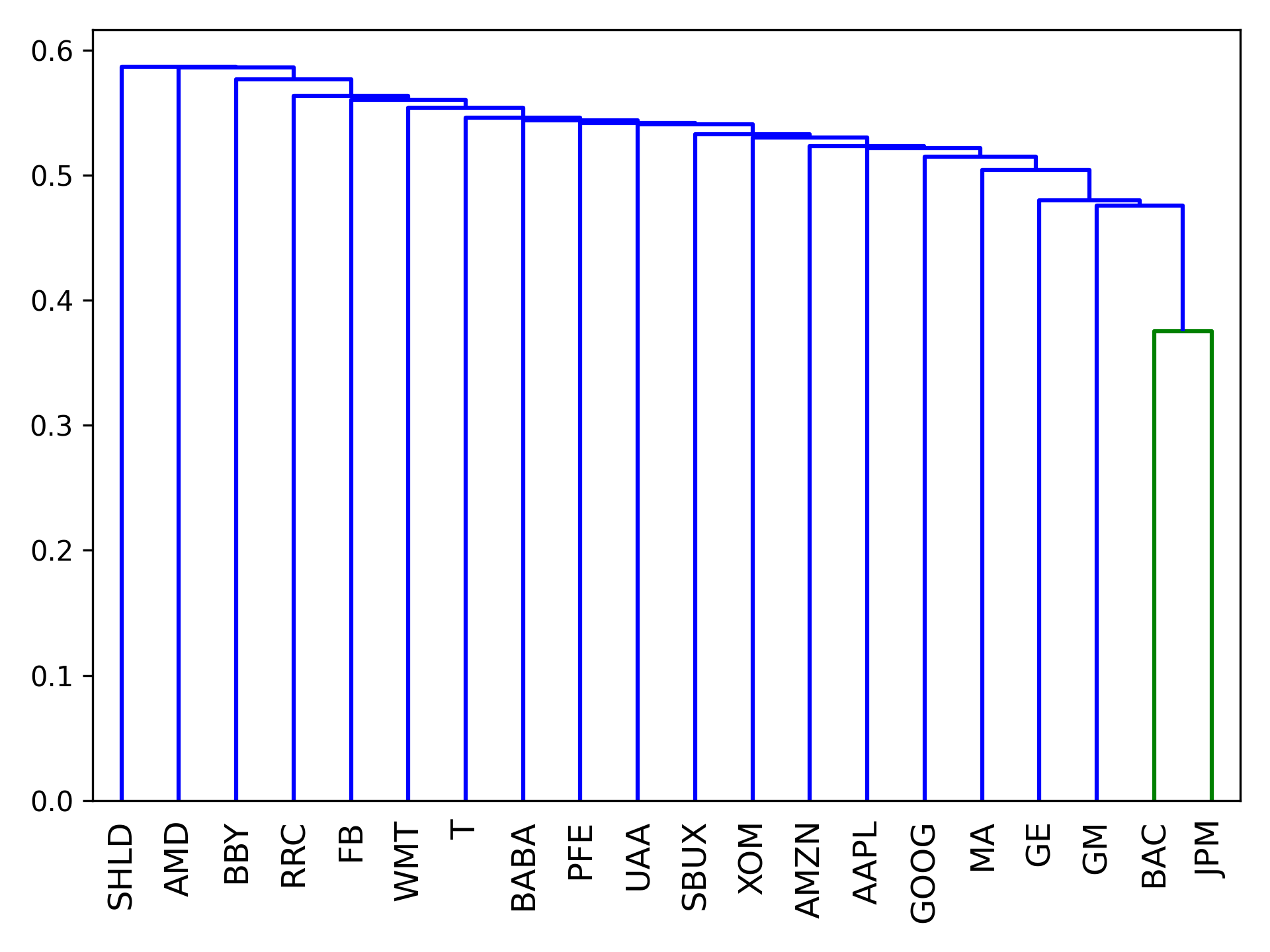](https://pyportfolioopt.readthedocs.io/en/stable/_images/dendrogram.png)
The `hierarchical_portfolio` module seeks to implement one of the recent advances in portfolio optimization – the application of hierarchical clustering models in allocation.
All of the hierarchical classes have a similar API to `EfficientFrontier`, though since many hierarchical models currently don’t support different objectives, the actual allocation happens with a call to optimize().
Currently implemented:
* `HRPOpt` implements the Hierarchical Risk Parity (HRP) portfolio. Code reproduced with permission from Marcos Lopez de Prado (2016).
_class_ `pypfopt.hierarchical_portfolio.``HRPOpt`(_returns=None_, _cov\_matrix=None_)[\[source\]](https://pyportfolioopt.readthedocs.io/en/stable/_modules/pypfopt/hierarchical_portfolio.html#HRPOpt)
[¶](https://pyportfolioopt.readthedocs.io/en/stable/OtherOptimizers.html#pypfopt.hierarchical_portfolio.HRPOpt "Permalink to this definition")
A HRPOpt object (inheriting from BaseOptimizer) constructs a hierarchical risk parity portfolio.
Instance variables:
* Inputs
> * `n_assets` - int
> * `tickers` - str list
> * `returns` - pd.DataFrame
* Output:
> * `weights` - np.ndarray
> * `clusters` - linkage matrix corresponding to clustered assets.
Public methods:
* `optimize()` calculates weights using HRP
* `portfolio_performance()` calculates the expected return, volatility and Sharpe ratio for the optimized portfolio.
* `set_weights()` creates self.weights (np.ndarray) from a weights dict
* `clean_weights()` rounds the weights and clips near-zeros.
* `save_weights_to_file()` saves the weights to csv, json, or txt.
`__init__`(_returns=None_, _cov\_matrix=None_)[\[source\]](https://pyportfolioopt.readthedocs.io/en/stable/_modules/pypfopt/hierarchical_portfolio.html#HRPOpt.__init__)
[¶](https://pyportfolioopt.readthedocs.io/en/stable/OtherOptimizers.html#pypfopt.hierarchical_portfolio.HRPOpt.__init__ "Permalink to this definition")
| | |
| --- | --- |
| Parameters: | * **returns** (_pd.DataFrame_) – asset historical returns
* **cov\_matrix** (_pd.DataFrame._) – covariance of asset returns |
| Raises: | **TypeError** – if `returns` is not a dataframe |
`optimize`(_linkage\_method='single'_)[\[source\]](https://pyportfolioopt.readthedocs.io/en/stable/_modules/pypfopt/hierarchical_portfolio.html#HRPOpt.optimize)
[¶](https://pyportfolioopt.readthedocs.io/en/stable/OtherOptimizers.html#pypfopt.hierarchical_portfolio.HRPOpt.optimize "Permalink to this definition")
Construct a hierarchical risk parity portfolio, using Scipy hierarchical clustering (see [here](https://docs.scipy.org/doc/scipy/reference/generated/scipy.cluster.hierarchy.linkage.html)
)
| | |
| --- | --- |
| Parameters: | **linkage\_method** (_str_) – which scipy linkage method to use |
| Returns: | weights for the HRP portfolio |
| Return type: | OrderedDict |
`portfolio_performance`(_verbose=False_, _risk\_free\_rate=0.02_, _frequency=252_)[\[source\]](https://pyportfolioopt.readthedocs.io/en/stable/_modules/pypfopt/hierarchical_portfolio.html#HRPOpt.portfolio_performance)
[¶](https://pyportfolioopt.readthedocs.io/en/stable/OtherOptimizers.html#pypfopt.hierarchical_portfolio.HRPOpt.portfolio_performance "Permalink to this definition")
After optimising, calculate (and optionally print) the performance of the optimal portfolio. Currently calculates expected return, volatility, and the Sharpe ratio assuming returns are daily
| | |
| --- | --- |
| Parameters: | * **verbose** (_bool__,_ _optional_) – whether performance should be printed, defaults to False
* **risk\_free\_rate** (_float__,_ _optional_) – risk-free rate of borrowing/lending, defaults to 0.02. The period of the risk-free rate should correspond to the frequency of expected returns.
* **frequency** (_int__,_ _optional_) – number of time periods in a year, defaults to 252 (the number of trading days in a year) |
| Raises: | **ValueError** – if weights have not been calculated yet |
| Returns: | expected return, volatility, Sharpe ratio. |
| Return type: | (float, float, float) |
The Critical Line Algorithm[¶](https://pyportfolioopt.readthedocs.io/en/stable/OtherOptimizers.html#the-critical-line-algorithm "Permalink to this headline")
--------------------------------------------------------------------------------------------------------------------------------------------------------------
This is a robust alternative to the quadratic solver used to find mean-variance optimal portfolios, that is especially advantageous when we apply linear inequalities. Unlike generic convex optimization routines, the CLA is specially designed for portfolio optimization. It is guaranteed to converge after a certain number of iterations, and can efficiently derive the entire efficient frontier.
[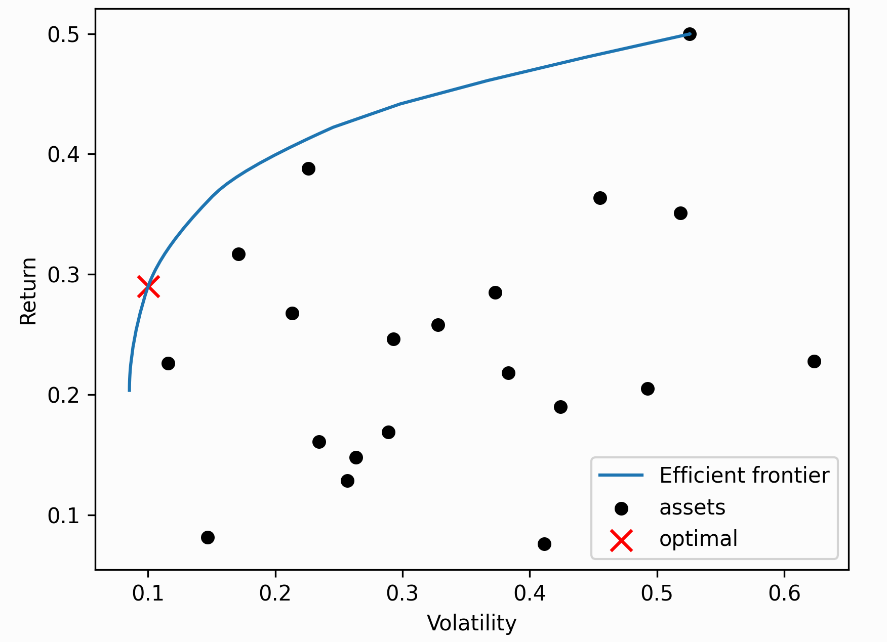](https://pyportfolioopt.readthedocs.io/en/stable/_images/cla_plot.png)
Tip
In general, unless you have specific requirements e.g you would like to efficiently compute the entire efficient frontier for plotting, I would go with the standard `EfficientFrontier` optimizer.
I am most grateful to Marcos López de Prado and David Bailey for providing the implementation [\[2\]](https://pyportfolioopt.readthedocs.io/en/stable/OtherOptimizers.html#id5)
. Permission for its distribution has been received by email. It has been modified such that it has the same API, though as of v0.5.0 we only support `max_sharpe()` and `min_volatility()`.
The `cla` module houses the CLA class, which generates optimal portfolios using the Critical Line Algorithm as implemented by Marcos Lopez de Prado and David Bailey.
_class_ `pypfopt.cla.``CLA`(_expected\_returns_, _cov\_matrix_, _weight\_bounds=(0_, _1)_)[\[source\]](https://pyportfolioopt.readthedocs.io/en/stable/_modules/pypfopt/cla.html#CLA)
[¶](https://pyportfolioopt.readthedocs.io/en/stable/OtherOptimizers.html#pypfopt.cla.CLA "Permalink to this definition")
Instance variables:
* Inputs:
> * `n_assets` - int
> * `tickers` - str list
> * `mean` - np.ndarray
> * `cov_matrix` - np.ndarray
> * `expected_returns` - np.ndarray
> * `lb` - np.ndarray
> * `ub` - np.ndarray
* Optimization parameters:
> * `w` - np.ndarray list
> * `ls` - float list
> * `g` - float list
> * `f` - float list list
* Outputs:
> * `weights` - np.ndarray
> * `frontier_values` - (float list, float list, np.ndarray list)
Public methods:
* `max_sharpe()` optimizes for maximal Sharpe ratio (a.k.a the tangency portfolio)
* `min_volatility()` optimizes for minimum volatility
* `efficient_frontier()` computes the entire efficient frontier
* `portfolio_performance()` calculates the expected return, volatility and Sharpe ratio for the optimized portfolio.
* `clean_weights()` rounds the weights and clips near-zeros.
* `save_weights_to_file()` saves the weights to csv, json, or txt.
`__init__`(_expected\_returns_, _cov\_matrix_, _weight\_bounds=(0_, _1)_)[\[source\]](https://pyportfolioopt.readthedocs.io/en/stable/_modules/pypfopt/cla.html#CLA.__init__)
[¶](https://pyportfolioopt.readthedocs.io/en/stable/OtherOptimizers.html#pypfopt.cla.CLA.__init__ "Permalink to this definition")
| | |
| --- | --- |
| Parameters: | * **expected\_returns** (_pd.Series__,_ _list__,_ _np.ndarray_) – expected returns for each asset. Set to None if optimising for volatility only.
* **cov\_matrix** (_pd.DataFrame_ _or_ _np.array_) – covariance of returns for each asset
* **weight\_bounds** (_tuple_ _(__float__,_ _float__) or_ _(__list/ndarray__,_ _list/ndarray__) or_ _list__(__tuple__(__float__,_ _float__)__)_) – minimum and maximum weight of an asset, defaults to (0, 1). Must be changed to (-1, 1) for portfolios with shorting. |
| Raises: | * **TypeError** – if `expected_returns` is not a series, list or array
* **TypeError** – if `cov_matrix` is not a dataframe or array |
`efficient_frontier`(_points=100_)[\[source\]](https://pyportfolioopt.readthedocs.io/en/stable/_modules/pypfopt/cla.html#CLA.efficient_frontier)
[¶](https://pyportfolioopt.readthedocs.io/en/stable/OtherOptimizers.html#pypfopt.cla.CLA.efficient_frontier "Permalink to this definition")
Efficiently compute the entire efficient frontier
| | |
| --- | --- |
| Parameters: | **points** (_int__,_ _optional_) – rough number of points to evaluate, defaults to 100 |
| Raises: | **ValueError** – if weights have not been computed |
| Returns: | return list, std list, weight list |
| Return type: | (float list, float list, np.ndarray list) |
`max_sharpe`()[\[source\]](https://pyportfolioopt.readthedocs.io/en/stable/_modules/pypfopt/cla.html#CLA.max_sharpe)
[¶](https://pyportfolioopt.readthedocs.io/en/stable/OtherOptimizers.html#pypfopt.cla.CLA.max_sharpe "Permalink to this definition")
Maximise the Sharpe ratio.
| | |
| --- | --- |
| Returns: | asset weights for the max-sharpe portfolio |
| Return type: | OrderedDict |
`min_volatility`()[\[source\]](https://pyportfolioopt.readthedocs.io/en/stable/_modules/pypfopt/cla.html#CLA.min_volatility)
[¶](https://pyportfolioopt.readthedocs.io/en/stable/OtherOptimizers.html#pypfopt.cla.CLA.min_volatility "Permalink to this definition")
Minimise volatility.
| | |
| --- | --- |
| Returns: | asset weights for the volatility-minimising portfolio |
| Return type: | OrderedDict |
`portfolio_performance`(_verbose=False_, _risk\_free\_rate=0.02_)[\[source\]](https://pyportfolioopt.readthedocs.io/en/stable/_modules/pypfopt/cla.html#CLA.portfolio_performance)
[¶](https://pyportfolioopt.readthedocs.io/en/stable/OtherOptimizers.html#pypfopt.cla.CLA.portfolio_performance "Permalink to this definition")
After optimising, calculate (and optionally print) the performance of the optimal portfolio. Currently calculates expected return, volatility, and the Sharpe ratio.
| | |
| --- | --- |
| Parameters: | * **verbose** (_bool__,_ _optional_) – whether performance should be printed, defaults to False
* **risk\_free\_rate** (_float__,_ _optional_) – risk-free rate of borrowing/lending, defaults to 0.02 |
| Raises: | **ValueError** – if weights have not been calculated yet |
| Returns: | expected return, volatility, Sharpe ratio. |
| Return type: | (float, float, float) |
`set_weights`(_\__)[\[source\]](https://pyportfolioopt.readthedocs.io/en/stable/_modules/pypfopt/cla.html#CLA.set_weights)
[¶](https://pyportfolioopt.readthedocs.io/en/stable/OtherOptimizers.html#pypfopt.cla.CLA.set_weights "Permalink to this definition")
Utility function to set weights attribute (np.array) from user input
| | |
| --- | --- |
| Parameters: | **input\_weights** (_dict_) – {ticker: weight} dict |
Implementing your own optimizer[¶](https://pyportfolioopt.readthedocs.io/en/stable/OtherOptimizers.html#implementing-your-own-optimizer "Permalink to this headline")
----------------------------------------------------------------------------------------------------------------------------------------------------------------------
Please note that this is quite different to implementing [Custom optimization problems](https://pyportfolioopt.readthedocs.io/en/stable/GeneralEfficientFrontier.html#custom-optimization)
, because in that case we are still using the same convex optimization structure. However, HRP and CLA optimization have a fundamentally different optimization method. In general, these are much more difficult to code up compared to custom objective functions.
To implement a custom optimizer that is compatible with the rest of PyPortfolioOpt, just extend `BaseOptimizer` (or `BaseConvexOptimizer` if you want to use `cvxpy`), both of which can be found in `base_optimizer.py`. This gives you access to utility methods like `clean_weights()`, as well as making sure that any output is compatible with `portfolio_performance()` and post-processing methods.
The `base_optimizer` module houses the parent classes `BaseOptimizer` from which all optimizers will inherit. `BaseConvexOptimizer` is the base class for all `cvxpy` (and `scipy`) optimization.
Additionally, we define a general utility function `portfolio_performance` to evaluate return and risk for a given set of portfolio weights.
_class_ `pypfopt.base_optimizer.``BaseOptimizer`(_n\_assets_, _tickers=None_)[\[source\]](https://pyportfolioopt.readthedocs.io/en/stable/_modules/pypfopt/base_optimizer.html#BaseOptimizer)
[¶](https://pyportfolioopt.readthedocs.io/en/stable/OtherOptimizers.html#pypfopt.base_optimizer.BaseOptimizer "Permalink to this definition")
Instance variables:
* `n_assets` - int
* `tickers` - str list
* `weights` - np.ndarray
Public methods:
* `set_weights()` creates self.weights (np.ndarray) from a weights dict
* `clean_weights()` rounds the weights and clips near-zeros.
* `save_weights_to_file()` saves the weights to csv, json, or txt.
`__init__`(_n\_assets_, _tickers=None_)[\[source\]](https://pyportfolioopt.readthedocs.io/en/stable/_modules/pypfopt/base_optimizer.html#BaseOptimizer.__init__)
[¶](https://pyportfolioopt.readthedocs.io/en/stable/OtherOptimizers.html#pypfopt.base_optimizer.BaseOptimizer.__init__ "Permalink to this definition")
| | |
| --- | --- |
| Parameters: | * **n\_assets** (_int_) – number of assets
* **tickers** (_list_) – name of assets |
`clean_weights`(_cutoff=0.0001_, _rounding=5_)[\[source\]](https://pyportfolioopt.readthedocs.io/en/stable/_modules/pypfopt/base_optimizer.html#BaseOptimizer.clean_weights)
[¶](https://pyportfolioopt.readthedocs.io/en/stable/OtherOptimizers.html#pypfopt.base_optimizer.BaseOptimizer.clean_weights "Permalink to this definition")
Helper method to clean the raw weights, setting any weights whose absolute values are below the cutoff to zero, and rounding the rest.
| | |
| --- | --- |
| Parameters: | * **cutoff** (_float__,_ _optional_) – the lower bound, defaults to 1e-4
* **rounding** (_int__,_ _optional_) – number of decimal places to round the weights, defaults to 5. Set to None if rounding is not desired. |
| Returns: | asset weights |
| Return type: | OrderedDict |
`save_weights_to_file`(_filename='weights.csv'_)[\[source\]](https://pyportfolioopt.readthedocs.io/en/stable/_modules/pypfopt/base_optimizer.html#BaseOptimizer.save_weights_to_file)
[¶](https://pyportfolioopt.readthedocs.io/en/stable/OtherOptimizers.html#pypfopt.base_optimizer.BaseOptimizer.save_weights_to_file "Permalink to this definition")
Utility method to save weights to a text file.
| | |
| --- | --- |
| Parameters: | **filename** (_str_) – name of file. Should be csv, json, or txt. |
`set_weights`(_input\_weights_)[\[source\]](https://pyportfolioopt.readthedocs.io/en/stable/_modules/pypfopt/base_optimizer.html#BaseOptimizer.set_weights)
[¶](https://pyportfolioopt.readthedocs.io/en/stable/OtherOptimizers.html#pypfopt.base_optimizer.BaseOptimizer.set_weights "Permalink to this definition")
Utility function to set weights attribute (np.array) from user input
| | |
| --- | --- |
| Parameters: | **input\_weights** (_dict_) – {ticker: weight} dict |
_class_ `pypfopt.base_optimizer.``BaseConvexOptimizer`(_n\_assets_, _tickers=None_, _weight\_bounds=(0_, _1)_, _solver=None_, _verbose=False_, _solver\_options=None_)[\[source\]](https://pyportfolioopt.readthedocs.io/en/stable/_modules/pypfopt/base_optimizer.html#BaseConvexOptimizer)
[¶](https://pyportfolioopt.readthedocs.io/en/stable/OtherOptimizers.html#pypfopt.base_optimizer.BaseConvexOptimizer "Permalink to this definition")
The BaseConvexOptimizer contains many private variables for use by `cvxpy`. For example, the immutable optimization variable for weights is stored as self.\_w. Interacting directly with these variables directly is discouraged.
Instance variables:
* `n_assets` - int
* `tickers` - str list
* `weights` - np.ndarray
* `_opt` - cp.Problem
* `_solver` - str
* `_solver_options` - {str: str} dict
Public methods:
* `add_objective()` adds a (convex) objective to the optimization problem
* `add_constraint()` adds a constraint to the optimization problem
* `convex_objective()` solves for a generic convex objective with linear constraints
* `nonconvex_objective()` solves for a generic nonconvex objective using the scipy backend. This is prone to getting stuck in local minima and is generally _not_ recommended.
* `set_weights()` creates self.weights (np.ndarray) from a weights dict
* `clean_weights()` rounds the weights and clips near-zeros.
* `save_weights_to_file()` saves the weights to csv, json, or txt.
`__init__`(_n\_assets_, _tickers=None_, _weight\_bounds=(0_, _1)_, _solver=None_, _verbose=False_, _solver\_options=None_)[\[source\]](https://pyportfolioopt.readthedocs.io/en/stable/_modules/pypfopt/base_optimizer.html#BaseConvexOptimizer.__init__)
[¶](https://pyportfolioopt.readthedocs.io/en/stable/OtherOptimizers.html#pypfopt.base_optimizer.BaseConvexOptimizer.__init__ "Permalink to this definition")
| | |
| --- | --- |
| Parameters: | * **weight\_bounds** (_tuple OR tuple list__,_ _optional_) – minimum and maximum weight of each asset OR single min/max pair if all identical, defaults to (0, 1). Must be changed to (-1, 1) for portfolios with shorting.
* **solver** (_str__,_ _optional. Defaults to "ECOS"_) – name of solver. list available solvers with: `cvxpy.installed_solvers()`
* **verbose** (_bool__,_ _optional_) – whether performance and debugging info should be printed, defaults to False
* **solver\_options** (_dict__,_ _optional_) – parameters for the given solver |
`_map_bounds_to_constraints`(_test\_bounds_)[\[source\]](https://pyportfolioopt.readthedocs.io/en/stable/_modules/pypfopt/base_optimizer.html#BaseConvexOptimizer._map_bounds_to_constraints)
[¶](https://pyportfolioopt.readthedocs.io/en/stable/OtherOptimizers.html#pypfopt.base_optimizer.BaseConvexOptimizer._map_bounds_to_constraints "Permalink to this definition")
Convert input bounds into a form acceptable by cvxpy and add to the constraints list.
| | |
| --- | --- |
| Parameters: | **test\_bounds** (_tuple OR list/tuple of tuples OR pair of np arrays_) – minimum and maximum weight of each asset OR single min/max pair if all identical OR pair of arrays corresponding to lower/upper bounds. defaults to (0, 1). |
| Raises: | **TypeError** – if `test_bounds` is not of the right type |
| Returns: | bounds suitable for cvxpy |
| Return type: | tuple pair of np.ndarray |
`_solve_cvxpy_opt_problem`()[\[source\]](https://pyportfolioopt.readthedocs.io/en/stable/_modules/pypfopt/base_optimizer.html#BaseConvexOptimizer._solve_cvxpy_opt_problem)
[¶](https://pyportfolioopt.readthedocs.io/en/stable/OtherOptimizers.html#pypfopt.base_optimizer.BaseConvexOptimizer._solve_cvxpy_opt_problem "Permalink to this definition")
Helper method to solve the cvxpy problem and check output, once objectives and constraints have been defined
| | |
| --- | --- |
| Raises: | **exceptions.OptimizationError** – if problem is not solvable by cvxpy |
`add_constraint`(_new\_constraint_)[\[source\]](https://pyportfolioopt.readthedocs.io/en/stable/_modules/pypfopt/base_optimizer.html#BaseConvexOptimizer.add_constraint)
[¶](https://pyportfolioopt.readthedocs.io/en/stable/OtherOptimizers.html#pypfopt.base_optimizer.BaseConvexOptimizer.add_constraint "Permalink to this definition")
Add a new constraint to the optimization problem. This constraint must satisfy DCP rules, i.e be either a linear equality constraint or convex inequality constraint.
Examples:
ef.add\_constraint(lambda x : x\[0\] \== 0.02)
ef.add\_constraint(lambda x : x \>= 0.01)
ef.add\_constraint(lambda x: x <= np.array(\[0.01, 0.08, ..., 0.5\]))
| | |
| --- | --- |
| Parameters: | **new\_constraint** – the constraint to be added |
`add_objective`(_new\_objective_, _\*\*kwargs_)[\[source\]](https://pyportfolioopt.readthedocs.io/en/stable/_modules/pypfopt/base_optimizer.html#BaseConvexOptimizer.add_objective)
[¶](https://pyportfolioopt.readthedocs.io/en/stable/OtherOptimizers.html#pypfopt.base_optimizer.BaseConvexOptimizer.add_objective "Permalink to this definition")
Add a new term into the objective function. This term must be convex, and built from cvxpy atomic functions.
Example:
def L1\_norm(w, k\=1):
return k \* cp.norm(w, 1)
ef.add\_objective(L1\_norm, k\=2)
| | |
| --- | --- |
| Parameters: | **new\_objective** (_cp.Expression_ _(__i.e function of cp.Variable__)_) – the objective to be added |
`add_sector_constraints`(_sector\_mapper_, _sector\_lower_, _sector\_upper_)[\[source\]](https://pyportfolioopt.readthedocs.io/en/stable/_modules/pypfopt/base_optimizer.html#BaseConvexOptimizer.add_sector_constraints)
[¶](https://pyportfolioopt.readthedocs.io/en/stable/OtherOptimizers.html#pypfopt.base_optimizer.BaseConvexOptimizer.add_sector_constraints "Permalink to this definition")
Adds constraints on the sum of weights of different groups of assets. Most commonly, these will be sector constraints e.g portfolio’s exposure to tech must be less than x%:
sector\_mapper \= {
"GOOG": "tech",
"FB": "tech",,
"XOM": "Oil/Gas",
"RRC": "Oil/Gas",
"MA": "Financials",
"JPM": "Financials",
}
sector\_lower \= {"tech": 0.1} \# at least 10% to tech
sector\_upper \= {
"tech": 0.4, \# less than 40% tech
"Oil/Gas": 0.1 # less than 10% oil and gas
}
| | |
| --- | --- |
| Parameters: | * **sector\_mapper** (_{str: str} dict_) – dict that maps tickers to sectors
* **sector\_lower** (_{str: float} dict_) – lower bounds for each sector
* **sector\_upper** (_{str:float} dict_) – upper bounds for each sector |
`convex_objective`(_custom\_objective_, _weights\_sum\_to\_one=True_, _\*\*kwargs_)[\[source\]](https://pyportfolioopt.readthedocs.io/en/stable/_modules/pypfopt/base_optimizer.html#BaseConvexOptimizer.convex_objective)
[¶](https://pyportfolioopt.readthedocs.io/en/stable/OtherOptimizers.html#pypfopt.base_optimizer.BaseConvexOptimizer.convex_objective "Permalink to this definition")
Optimize a custom convex objective function. Constraints should be added with `ef.add_constraint()`. Optimizer arguments must be passed as keyword-args. Example:
\# Could define as a lambda function instead
def logarithmic\_barrier(w, cov\_matrix, k\=0.1):
\# 60 Years of Portfolio Optimization, Kolm et al (2014)
return cp.quad\_form(w, cov\_matrix) \- k \* cp.sum(cp.log(w))
w \= ef.convex\_objective(logarithmic\_barrier, cov\_matrix\=ef.cov\_matrix)
| | |
| --- | --- |
| Parameters: | * **custom\_objective** (function with signature (cp.Variable, \*\*kwargs) -> cp.Expression) – an objective function to be MINIMISED. This should be written using cvxpy atoms Should map (w, \*\*kwargs) -> float.
* **weights\_sum\_to\_one** (_bool__,_ _optional_) – whether to add the default objective, defaults to True |
| Raises: | **OptimizationError** – if the objective is nonconvex or constraints nonlinear. |
| Returns: | asset weights for the efficient risk portfolio |
| Return type: | OrderedDict |
`nonconvex_objective`(_custom\_objective_, _objective\_args=None_, _weights\_sum\_to\_one=True_, _constraints=None_, _solver='SLSQP'_, _initial\_guess=None_)[\[source\]](https://pyportfolioopt.readthedocs.io/en/stable/_modules/pypfopt/base_optimizer.html#BaseConvexOptimizer.nonconvex_objective)
[¶](https://pyportfolioopt.readthedocs.io/en/stable/OtherOptimizers.html#pypfopt.base_optimizer.BaseConvexOptimizer.nonconvex_objective "Permalink to this definition")
Optimize some objective function using the scipy backend. This can support nonconvex objectives and nonlinear constraints, but may get stuck at local minima. Example:
\# Market-neutral efficient risk
constraints \= \[\
{"type": "eq", "fun": lambda w: np.sum(w)}, \# weights sum to zero\
{\
"type": "eq",\
"fun": lambda w: target\_risk \*\* 2 \- np.dot(w.T, np.dot(ef.cov\_matrix, w)),\
}, \# risk = target\_risk\
\]
ef.nonconvex\_objective(
lambda w, mu: \-w.T.dot(mu), \# min negative return (i.e maximise return)
objective\_args\=(ef.expected\_returns,),
weights\_sum\_to\_one\=False,
constraints\=constraints,
)
| | |
| --- | --- |
| Parameters: | * **objective\_function** (_function with signature_ _(__np.ndarray__,_ _args__)_ _\-> float_) – an objective function to be MINIMISED. This function should map (weight, args) -> cost
* **objective\_args** (_tuple of np.ndarrays_) – arguments for the objective function (excluding weight)
* **weights\_sum\_to\_one** (_bool__,_ _optional_) – whether to add the default objective, defaults to True
* **constraints** (_dict list_) – list of constraints in the scipy format (i.e dicts)
* **solver** (_string_) – which SCIPY solver to use, e.g “SLSQP”, “COBYLA”, “BFGS”. User beware: different optimizers require different inputs.
* **initial\_guess** (_np.ndarray_) – the initial guess for the weights, shape (n,) or (n, 1) |
| Returns: | asset weights that optimize the custom objective |
| Return type: | OrderedDict |
References[¶](https://pyportfolioopt.readthedocs.io/en/stable/OtherOptimizers.html#references "Permalink to this headline")
----------------------------------------------------------------------------------------------------------------------------
| | |
| --- | --- |
| [\[1\]](https://pyportfolioopt.readthedocs.io/en/stable/OtherOptimizers.html#id2) | López de Prado, M. (2016). [Building Diversified Portfolios that Outperform Out of Sample](https://papers.ssrn.com/sol3/papers.cfm?abstract_id=2708678)
. The Journal of Portfolio Management, 42(4), 59–69. |
| | |
| --- | --- |
| [\[2\]](https://pyportfolioopt.readthedocs.io/en/stable/OtherOptimizers.html#id3) | Bailey and Loópez de Prado (2013). [An Open-Source Implementation of the Critical-Line Algorithm for Portfolio Optimization](https://papers.ssrn.com/sol3/papers.cfm?abstract_id=2197616) |
---
# Post-processing weights — PyPortfolioOpt 1.4.1 documentation
* [Docs](https://pyportfolioopt.readthedocs.io/en/stable/index.html)
»
* Post-processing weights
* [Edit on GitHub](https://github.com/robertmartin8/PyPortfolioOpt/blob/1db089602dee348f1eade9b981ca21cd35f1dcca/docs/Postprocessing.rst)
* * *
Post-processing weights[¶](https://pyportfolioopt.readthedocs.io/en/stable/Postprocessing.html#post-processing-weights "Permalink to this headline")
=====================================================================================================================================================
After optimal weights have been generated, it is often necessary to do some post-processing before they can be used practically. In particular, you are likely using portfolio optimization techniques to generate a **portfolio allocation** – a list of tickers and corresponding integer quantities that you could go and purchase at a broker.
However, it is not trivial to convert the continuous weights (output by any of our optimization methods) into an actionable allocation. For example, let us say that we have $10,000 that we would like to allocate. If we multiply the weights by this total portfolio value, the result will be dollar amounts of each asset. So if the optimal weight for Apple is 0.15, we need $1500 worth of Apple stock. However, Apple shares come in discrete units ($190 at the time of writing), so we will not be able to buy exactly $1500 of stock. The best we can do is to buy the number of shares that gets us closest to the desired dollar value.
PyPortfolioOpt offers two ways of solving this problem: one using a simple greedy algorithm, the other using integer programming.
Greedy algorithm[¶](https://pyportfolioopt.readthedocs.io/en/stable/Postprocessing.html#greedy-algorithm "Permalink to this headline")
---------------------------------------------------------------------------------------------------------------------------------------
`DiscreteAllocation.greedy_portfolio()` proceeds in two ‘rounds’. In the first round, we buy as many shares as we can for each asset without going over the desired weight. In the Apple example, \\(1500/190 \\approx 7.89\\), so we buy 7 shares at a cost of $1330. After iterating through all of the assets, we will have a lot of money left over (since we always rounded down).
In the second round, we calculate how far the current weights deviate from the existing weights for each asset. We wanted Apple to form 15% of the portfolio (with total value $10,000), but we only bought $1330 worth of Apple stock, so there is a deviation of \\(0.15 - 0.133\\). Some assets will have a higher deviation from the ideal, so we will purchase shares of these first. We then repeat the process, always buying shares of the asset whose current weight is furthest away from the ideal weight. Though this algorithm will not guarantee the optimal solution, I have found that it allows us to generate discrete allocations with very little money left over (e.g $12 left on a $10,000 portfolio).
That being said, we can see that on the test dataset (for a standard `max_sharpe` portfolio), the allocation method may deviate rather widely from the desired weights, particularly for companies with a high share price (e.g AMZN).
Funds remaining: 12.15
MA: allocated 0.242, desired 0.246
FB: allocated 0.200, desired 0.199
PFE: allocated 0.183, desired 0.184
BABA: allocated 0.088, desired 0.096
AAPL: allocated 0.086, desired 0.092
AMZN: allocated 0.000, desired 0.072
BBY: allocated 0.064, desired 0.061
SBUX: allocated 0.036, desired 0.038
GOOG: allocated 0.102, desired 0.013
Allocation has RMSE: 0.038
Integer programming[¶](https://pyportfolioopt.readthedocs.io/en/stable/Postprocessing.html#integer-programming "Permalink to this headline")
---------------------------------------------------------------------------------------------------------------------------------------------
This method (credit to [Dingyuan Wang](https://github.com/gumblex)
for the first implementation) treats the discrete allocation as an integer programming problem. In effect, the integer programming approach searches the space of possible allocations to find the one that is closest to our desired weights. We will use the following notation:
* \\(T \\in \\mathbb{R}\\) is the total dollar value to be allocated
* \\(p \\in \\mathbb{R}^n\\) is the array of latest prices
* \\(w \\in \\mathbb{R}^n\\) is the set of target weights
* \\(x \\in \\mathbb{Z}^n\\) is the integer allocation (i.e the result)
* \\(r \\in \\mathbb{R}\\) is the remaining unallocated value, i.e \\(r = T - x \\cdot p\\).
The optimization problem is then given by:
\\\[\\begin{split}\\begin{equation\*} \\begin{aligned} & \\underset{x \\in \\mathbb{Z}^n}{\\text{minimise}} & & r + \\lVert wT - x \\odot p \\rVert\_1 \\\\ & \\text{subject to} & & r + x \\cdot p = T\\\\ \\end{aligned} \\end{equation\*}\\end{split}\\\]
This is straightforward to translate into `cvxpy`.
Caution
Though `lp_portfolio()` produces allocations with a lower RMSE, some testing shows that it is between 100 and 1000 times slower than `greedy_portfolio()`. This doesn’t matter for small portfolios (it should still take less than a second), but the runtime for integer programs grows exponentially as the number of stocks, so for large portfolios you may have to use `greedy_portfolio()`.
Dealing with shorts[¶](https://pyportfolioopt.readthedocs.io/en/stable/Postprocessing.html#dealing-with-shorts "Permalink to this headline")
---------------------------------------------------------------------------------------------------------------------------------------------
As of v0.4, `DiscreteAllocation` automatically deals with shorts by finding separate discrete allocations for the long-only and short-only portions. If your portfolio has shorts, you should pass a short ratio. The default is 0.30, corresponding to a 130/30 long-short balance. Practically, this means that you would go long $10,000 of some stocks, short $3000 of some other stocks, then use the proceeds from the shorts to go long another $3000. Thus the total value of the resulting portfolio would be $13,000.
Documentation reference[¶](https://pyportfolioopt.readthedocs.io/en/stable/Postprocessing.html#module-pypfopt.discrete_allocation "Permalink to this headline")
----------------------------------------------------------------------------------------------------------------------------------------------------------------
The `discrete_allocation` module contains the `DiscreteAllocation` class, which offers multiple methods to generate a discrete portfolio allocation from continuous weights.
_class_ `pypfopt.discrete_allocation.``DiscreteAllocation`(_weights_, _latest\_prices_, _total\_portfolio\_value=10000_, _short\_ratio=None_)[\[source\]](https://pyportfolioopt.readthedocs.io/en/stable/_modules/pypfopt/discrete_allocation.html#DiscreteAllocation)
[¶](https://pyportfolioopt.readthedocs.io/en/stable/Postprocessing.html#pypfopt.discrete_allocation.DiscreteAllocation "Permalink to this definition")
Generate a discrete portfolio allocation from continuous weights
Instance variables:
* Inputs:
> * `weights` - dict
> * `latest_prices` - pd.Series or dict
> * `total_portfolio_value` - int/float
> * `short_ratio`\- float
* Output: `allocation` - dict
Public methods:
* `greedy_portfolio()` - uses a greedy algorithm
* `lp_portfolio()` - uses linear programming
`__init__`(_weights_, _latest\_prices_, _total\_portfolio\_value=10000_, _short\_ratio=None_)[\[source\]](https://pyportfolioopt.readthedocs.io/en/stable/_modules/pypfopt/discrete_allocation.html#DiscreteAllocation.__init__)
[¶](https://pyportfolioopt.readthedocs.io/en/stable/Postprocessing.html#pypfopt.discrete_allocation.DiscreteAllocation.__init__ "Permalink to this definition")
| | |
| --- | --- |
| Parameters: | * **weights** (_dict_) – continuous weights generated from the `efficient_frontier` module
* **latest\_prices** (_pd.Series_) – the most recent price for each asset
* **total\_portfolio\_value** (_int/float__,_ _optional_) – the desired total value of the portfolio, defaults to 10000
* **short\_ratio** (_float__,_ _defaults to None._) – the short ratio, e.g 0.3 corresponds to 130/30. If None, defaults to the input weights. |
| Raises: | * **TypeError** – if `weights` is not a dict
* **TypeError** – if `latest_prices` isn’t a series
* **ValueError** – if `short_ratio < 0` |
`_allocation_rmse_error`(_verbose=True_)[\[source\]](https://pyportfolioopt.readthedocs.io/en/stable/_modules/pypfopt/discrete_allocation.html#DiscreteAllocation._allocation_rmse_error)
[¶](https://pyportfolioopt.readthedocs.io/en/stable/Postprocessing.html#pypfopt.discrete_allocation.DiscreteAllocation._allocation_rmse_error "Permalink to this definition")
Utility function to calculate and print RMSE error between discretised weights and continuous weights. RMSE was used instead of MAE because we want to penalise large variations.
| | |
| --- | --- |
| Parameters: | **verbose** (_bool_) – print weight discrepancies? |
| Returns: | rmse error |
| Return type: | float |
_static_ `_remove_zero_positions`(_allocation_)[\[source\]](https://pyportfolioopt.readthedocs.io/en/stable/_modules/pypfopt/discrete_allocation.html#DiscreteAllocation._remove_zero_positions)
[¶](https://pyportfolioopt.readthedocs.io/en/stable/Postprocessing.html#pypfopt.discrete_allocation.DiscreteAllocation._remove_zero_positions "Permalink to this definition")
Utility function to remove zero positions (i.e with no shares being bought)
`greedy_portfolio`(_reinvest=False_, _verbose=False_)[\[source\]](https://pyportfolioopt.readthedocs.io/en/stable/_modules/pypfopt/discrete_allocation.html#DiscreteAllocation.greedy_portfolio)
[¶](https://pyportfolioopt.readthedocs.io/en/stable/Postprocessing.html#pypfopt.discrete_allocation.DiscreteAllocation.greedy_portfolio "Permalink to this definition")
Convert continuous weights into a discrete portfolio allocation using a greedy iterative approach.
| | |
| --- | --- |
| Parameters: | * **reinvest** (_bool__,_ _defaults to False_) – whether or not to reinvest cash gained from shorting
* **verbose** (_bool__,_ _defaults to False_) – print error analysis? |
| Returns: | the number of shares of each ticker that should be purchased, along with the amount of funds leftover. |
| Return type: | (dict, float) |
`lp_portfolio`(_reinvest=False_, _verbose=False_, _solver='GLPK\_MI'_)[\[source\]](https://pyportfolioopt.readthedocs.io/en/stable/_modules/pypfopt/discrete_allocation.html#DiscreteAllocation.lp_portfolio)
[¶](https://pyportfolioopt.readthedocs.io/en/stable/Postprocessing.html#pypfopt.discrete_allocation.DiscreteAllocation.lp_portfolio "Permalink to this definition")
Convert continuous weights into a discrete portfolio allocation using integer programming.
| | |
| --- | --- |
| Parameters: | * **reinvest** (_bool__,_ _defaults to False_) – whether or not to reinvest cash gained from shorting
* **verbose** (_bool_) – print error analysis?
* **solver** (_str__,_ _defaults to "GLPK\_MI"_) – the CVXPY solver to use (must support mixed-integer programs) |
| Returns: | the number of shares of each ticker that should be purchased, along with the amount of funds leftover. |
| Return type: | (dict, float) |
---
# Other Optimizers — PyPortfolioOpt 1.5.4 documentation
* [Docs](https://pyportfolioopt.readthedocs.io/en/latest/index.html)
»
* Other Optimizers
* [Edit on GitHub](https://github.com/robertmartin8/PyPortfolioOpt/blob/master/docs/OtherOptimizers.rst)
* * *
Other Optimizers[¶](https://pyportfolioopt.readthedocs.io/en/latest/OtherOptimizers.html#other-optimizers "Permalink to this headline")
========================================================================================================================================
Efficient frontier methods involve the direct optimization of an objective subject to constraints. However, there are some portfolio optimization schemes that are completely different in character. PyPortfolioOpt provides support for these alternatives, while still giving you access to the same pre and post-processing API.
Note
As of v0.4, these other optimizers now inherit from `BaseOptimizer` or `BaseConvexOptimizer`, so you no longer have to implement pre-processing and post-processing methods on your own. You can thus easily swap out, say, `EfficientFrontier` for `HRPOpt`.
Hierarchical Risk Parity (HRP)[¶](https://pyportfolioopt.readthedocs.io/en/latest/OtherOptimizers.html#hierarchical-risk-parity-hrp "Permalink to this headline")
------------------------------------------------------------------------------------------------------------------------------------------------------------------
Hierarchical Risk Parity is a novel portfolio optimization method developed by Marcos Lopez de Prado [\[1\]](https://pyportfolioopt.readthedocs.io/en/latest/OtherOptimizers.html#id4)
. Though a detailed explanation can be found in the linked paper, here is a rough overview of how HRP works:
1. From a universe of assets, form a distance matrix based on the correlation of the assets.
2. Using this distance matrix, cluster the assets into a tree via hierarchical clustering
3. Within each branch of the tree, form the minimum variance portfolio (normally between just two assets).
4. Iterate over each level, optimally combining the mini-portfolios at each node.
The advantages of this are that it does not require the inversion of the covariance matrix as with traditional mean-variance optimization, and seems to produce diverse portfolios that perform well out of sample.
[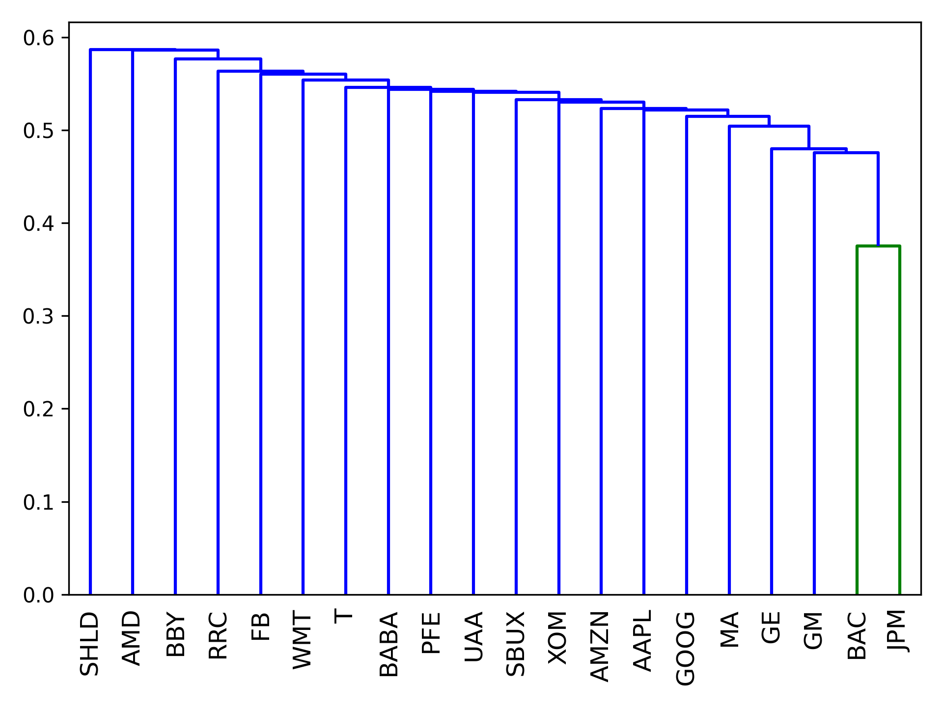](https://pyportfolioopt.readthedocs.io/en/latest/_images/dendrogram.png)
The `hierarchical_portfolio` module seeks to implement one of the recent advances in portfolio optimization – the application of hierarchical clustering models in allocation.
All of the hierarchical classes have a similar API to `EfficientFrontier`, though since many hierarchical models currently don’t support different objectives, the actual allocation happens with a call to optimize().
Currently implemented:
* `HRPOpt` implements the Hierarchical Risk Parity (HRP) portfolio. Code reproduced with permission from Marcos Lopez de Prado (2016).
_class_ `pypfopt.hierarchical_portfolio.``HRPOpt`(_returns=None_, _cov\_matrix=None_)[\[source\]](https://pyportfolioopt.readthedocs.io/en/latest/_modules/pypfopt/hierarchical_portfolio.html#HRPOpt)
[¶](https://pyportfolioopt.readthedocs.io/en/latest/OtherOptimizers.html#pypfopt.hierarchical_portfolio.HRPOpt "Permalink to this definition")
A HRPOpt object (inheriting from BaseOptimizer) constructs a hierarchical risk parity portfolio.
Instance variables:
* Inputs
> * `n_assets` - int
> * `tickers` - str list
> * `returns` - pd.DataFrame
* Output:
> * `weights` - np.ndarray
> * `clusters` - linkage matrix corresponding to clustered assets.
Public methods:
* `optimize()` calculates weights using HRP
* `portfolio_performance()` calculates the expected return, volatility and Sharpe ratio for the optimized portfolio.
* `set_weights()` creates self.weights (np.ndarray) from a weights dict
* `clean_weights()` rounds the weights and clips near-zeros.
* `save_weights_to_file()` saves the weights to csv, json, or txt.
`__init__`(_returns=None_, _cov\_matrix=None_)[\[source\]](https://pyportfolioopt.readthedocs.io/en/latest/_modules/pypfopt/hierarchical_portfolio.html#HRPOpt.__init__)
[¶](https://pyportfolioopt.readthedocs.io/en/latest/OtherOptimizers.html#pypfopt.hierarchical_portfolio.HRPOpt.__init__ "Permalink to this definition")
| | |
| --- | --- |
| Parameters: | * **returns** (_pd.DataFrame_) – asset historical returns
* **cov\_matrix** (_pd.DataFrame._) – covariance of asset returns |
| Raises: | **TypeError** – if `returns` is not a dataframe |
`optimize`(_linkage\_method='single'_)[\[source\]](https://pyportfolioopt.readthedocs.io/en/latest/_modules/pypfopt/hierarchical_portfolio.html#HRPOpt.optimize)
[¶](https://pyportfolioopt.readthedocs.io/en/latest/OtherOptimizers.html#pypfopt.hierarchical_portfolio.HRPOpt.optimize "Permalink to this definition")
Construct a hierarchical risk parity portfolio, using Scipy hierarchical clustering (see [here](https://docs.scipy.org/doc/scipy/reference/generated/scipy.cluster.hierarchy.linkage.html)
)
| | |
| --- | --- |
| Parameters: | **linkage\_method** (_str_) – which scipy linkage method to use |
| Returns: | weights for the HRP portfolio |
| Return type: | OrderedDict |
`portfolio_performance`(_verbose=False_, _risk\_free\_rate=0.02_, _frequency=252_)[\[source\]](https://pyportfolioopt.readthedocs.io/en/latest/_modules/pypfopt/hierarchical_portfolio.html#HRPOpt.portfolio_performance)
[¶](https://pyportfolioopt.readthedocs.io/en/latest/OtherOptimizers.html#pypfopt.hierarchical_portfolio.HRPOpt.portfolio_performance "Permalink to this definition")
After optimising, calculate (and optionally print) the performance of the optimal portfolio. Currently calculates expected return, volatility, and the Sharpe ratio assuming returns are daily
| | |
| --- | --- |
| Parameters: | * **verbose** (_bool__,_ _optional_) – whether performance should be printed, defaults to False
* **risk\_free\_rate** (_float__,_ _optional_) – risk-free rate of borrowing/lending, defaults to 0.02. The period of the risk-free rate should correspond to the frequency of expected returns.
* **frequency** (_int__,_ _optional_) – number of time periods in a year, defaults to 252 (the number of trading days in a year) |
| Raises: | **ValueError** – if weights have not been calculated yet |
| Returns: | expected return, volatility, Sharpe ratio. |
| Return type: | (float, float, float) |
The Critical Line Algorithm[¶](https://pyportfolioopt.readthedocs.io/en/latest/OtherOptimizers.html#the-critical-line-algorithm "Permalink to this headline")
--------------------------------------------------------------------------------------------------------------------------------------------------------------
This is a robust alternative to the quadratic solver used to find mean-variance optimal portfolios, that is especially advantageous when we apply linear inequalities. Unlike generic convex optimization routines, the CLA is specially designed for portfolio optimization. It is guaranteed to converge after a certain number of iterations, and can efficiently derive the entire efficient frontier.
[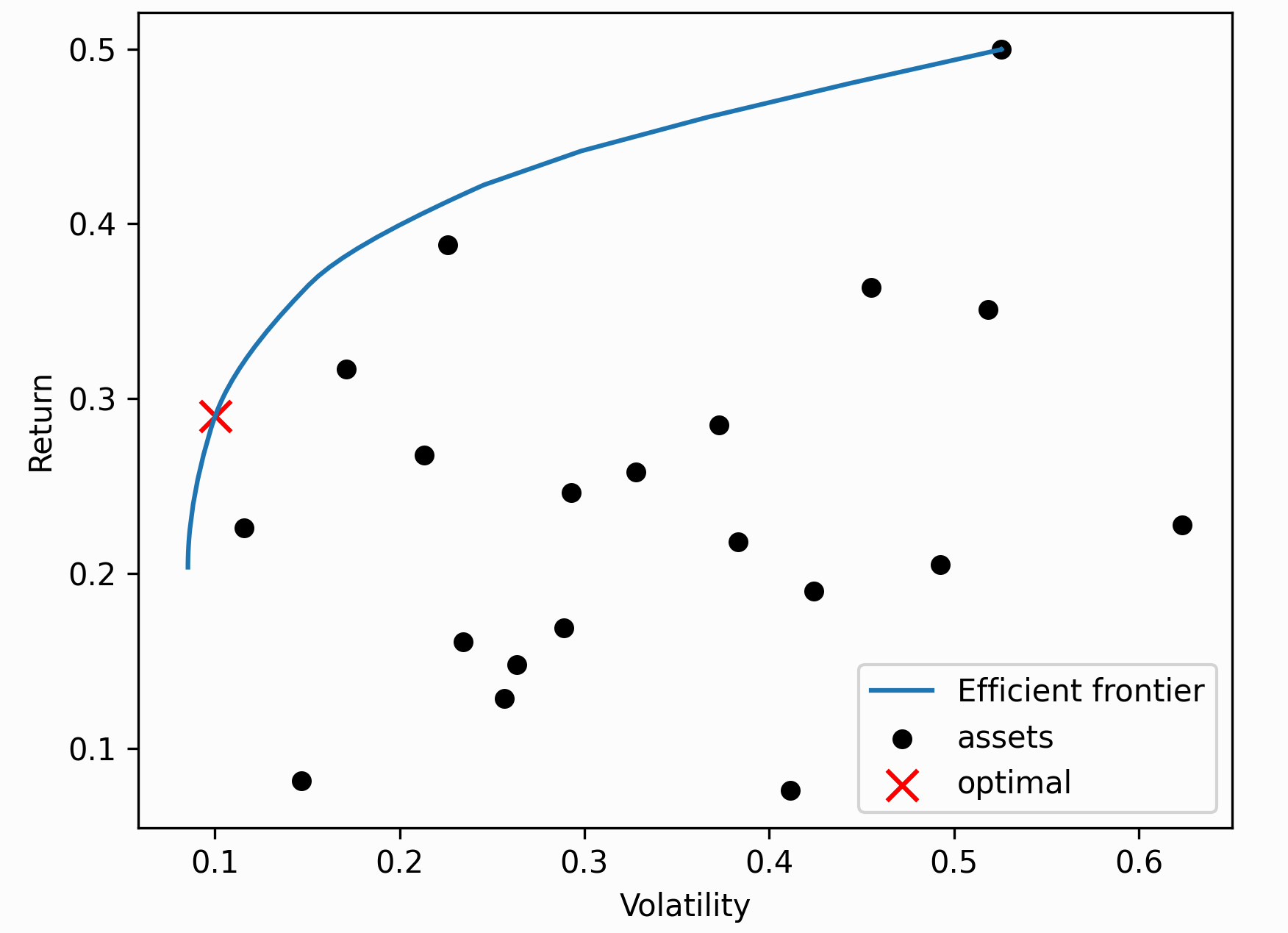](https://pyportfolioopt.readthedocs.io/en/latest/_images/cla_plot.png)
Tip
In general, unless you have specific requirements e.g you would like to efficiently compute the entire efficient frontier for plotting, I would go with the standard `EfficientFrontier` optimizer.
I am most grateful to Marcos López de Prado and David Bailey for providing the implementation [\[2\]](https://pyportfolioopt.readthedocs.io/en/latest/OtherOptimizers.html#id5)
. Permission for its distribution has been received by email. It has been modified such that it has the same API, though as of v0.5.0 we only support `max_sharpe()` and `min_volatility()`.
The `cla` module houses the CLA class, which generates optimal portfolios using the Critical Line Algorithm as implemented by Marcos Lopez de Prado and David Bailey.
_class_ `pypfopt.cla.``CLA`(_expected\_returns_, _cov\_matrix_, _weight\_bounds=(0_, _1)_)[\[source\]](https://pyportfolioopt.readthedocs.io/en/latest/_modules/pypfopt/cla.html#CLA)
[¶](https://pyportfolioopt.readthedocs.io/en/latest/OtherOptimizers.html#pypfopt.cla.CLA "Permalink to this definition")
Instance variables:
* Inputs:
> * `n_assets` - int
> * `tickers` - str list
> * `mean` - np.ndarray
> * `cov_matrix` - np.ndarray
> * `expected_returns` - np.ndarray
> * `lb` - np.ndarray
> * `ub` - np.ndarray
* Optimization parameters:
> * `w` - np.ndarray list
> * `ls` - float list
> * `g` - float list
> * `f` - float list list
* Outputs:
> * `weights` - np.ndarray
> * `frontier_values` - (float list, float list, np.ndarray list)
Public methods:
* `max_sharpe()` optimizes for maximal Sharpe ratio (a.k.a the tangency portfolio)
* `min_volatility()` optimizes for minimum volatility
* `efficient_frontier()` computes the entire efficient frontier
* `portfolio_performance()` calculates the expected return, volatility and Sharpe ratio for the optimized portfolio.
* `clean_weights()` rounds the weights and clips near-zeros.
* `save_weights_to_file()` saves the weights to csv, json, or txt.
`__init__`(_expected\_returns_, _cov\_matrix_, _weight\_bounds=(0_, _1)_)[\[source\]](https://pyportfolioopt.readthedocs.io/en/latest/_modules/pypfopt/cla.html#CLA.__init__)
[¶](https://pyportfolioopt.readthedocs.io/en/latest/OtherOptimizers.html#pypfopt.cla.CLA.__init__ "Permalink to this definition")
| | |
| --- | --- |
| Parameters: | * **expected\_returns** (_pd.Series__,_ _list__,_ _np.ndarray_) – expected returns for each asset. Set to None if optimising for volatility only.
* **cov\_matrix** (_pd.DataFrame_ _or_ _np.array_) – covariance of returns for each asset
* **weight\_bounds** (_tuple_ _(__float__,_ _float__) or_ _(__list/ndarray__,_ _list/ndarray__) or_ _list__(__tuple__(__float__,_ _float__)__)_) – minimum and maximum weight of an asset, defaults to (0, 1). Must be changed to (-1, 1) for portfolios with shorting. |
| Raises: | * **TypeError** – if `expected_returns` is not a series, list or array
* **TypeError** – if `cov_matrix` is not a dataframe or array |
`efficient_frontier`(_points=100_)[\[source\]](https://pyportfolioopt.readthedocs.io/en/latest/_modules/pypfopt/cla.html#CLA.efficient_frontier)
[¶](https://pyportfolioopt.readthedocs.io/en/latest/OtherOptimizers.html#pypfopt.cla.CLA.efficient_frontier "Permalink to this definition")
Efficiently compute the entire efficient frontier
| | |
| --- | --- |
| Parameters: | **points** (_int__,_ _optional_) – rough number of points to evaluate, defaults to 100 |
| Raises: | **ValueError** – if weights have not been computed |
| Returns: | return list, std list, weight list |
| Return type: | (float list, float list, np.ndarray list) |
`max_sharpe`()[\[source\]](https://pyportfolioopt.readthedocs.io/en/latest/_modules/pypfopt/cla.html#CLA.max_sharpe)
[¶](https://pyportfolioopt.readthedocs.io/en/latest/OtherOptimizers.html#pypfopt.cla.CLA.max_sharpe "Permalink to this definition")
Maximise the Sharpe ratio.
| | |
| --- | --- |
| Returns: | asset weights for the max-sharpe portfolio |
| Return type: | OrderedDict |
`min_volatility`()[\[source\]](https://pyportfolioopt.readthedocs.io/en/latest/_modules/pypfopt/cla.html#CLA.min_volatility)
[¶](https://pyportfolioopt.readthedocs.io/en/latest/OtherOptimizers.html#pypfopt.cla.CLA.min_volatility "Permalink to this definition")
Minimise volatility.
| | |
| --- | --- |
| Returns: | asset weights for the volatility-minimising portfolio |
| Return type: | OrderedDict |
`portfolio_performance`(_verbose=False_, _risk\_free\_rate=0.02_)[\[source\]](https://pyportfolioopt.readthedocs.io/en/latest/_modules/pypfopt/cla.html#CLA.portfolio_performance)
[¶](https://pyportfolioopt.readthedocs.io/en/latest/OtherOptimizers.html#pypfopt.cla.CLA.portfolio_performance "Permalink to this definition")
After optimising, calculate (and optionally print) the performance of the optimal portfolio. Currently calculates expected return, volatility, and the Sharpe ratio.
| | |
| --- | --- |
| Parameters: | * **verbose** (_bool__,_ _optional_) – whether performance should be printed, defaults to False
* **risk\_free\_rate** (_float__,_ _optional_) – risk-free rate of borrowing/lending, defaults to 0.02 |
| Raises: | **ValueError** – if weights have not been calculated yet |
| Returns: | expected return, volatility, Sharpe ratio. |
| Return type: | (float, float, float) |
`set_weights`(_\__)[\[source\]](https://pyportfolioopt.readthedocs.io/en/latest/_modules/pypfopt/cla.html#CLA.set_weights)
[¶](https://pyportfolioopt.readthedocs.io/en/latest/OtherOptimizers.html#pypfopt.cla.CLA.set_weights "Permalink to this definition")
Utility function to set weights attribute (np.array) from user input
| | |
| --- | --- |
| Parameters: | **input\_weights** (_dict_) – {ticker: weight} dict |
Implementing your own optimizer[¶](https://pyportfolioopt.readthedocs.io/en/latest/OtherOptimizers.html#implementing-your-own-optimizer "Permalink to this headline")
----------------------------------------------------------------------------------------------------------------------------------------------------------------------
Please note that this is quite different to implementing [Custom optimization problems](https://pyportfolioopt.readthedocs.io/en/latest/GeneralEfficientFrontier.html#custom-optimization)
, because in that case we are still using the same convex optimization structure. However, HRP and CLA optimization have a fundamentally different optimization method. In general, these are much more difficult to code up compared to custom objective functions.
To implement a custom optimizer that is compatible with the rest of PyPortfolioOpt, just extend `BaseOptimizer` (or `BaseConvexOptimizer` if you want to use `cvxpy`), both of which can be found in `base_optimizer.py`. This gives you access to utility methods like `clean_weights()`, as well as making sure that any output is compatible with `portfolio_performance()` and post-processing methods.
The `base_optimizer` module houses the parent classes `BaseOptimizer` from which all optimizers will inherit. `BaseConvexOptimizer` is the base class for all `cvxpy` (and `scipy`) optimization.
Additionally, we define a general utility function `portfolio_performance` to evaluate return and risk for a given set of portfolio weights.
_class_ `pypfopt.base_optimizer.``BaseOptimizer`(_n\_assets_, _tickers=None_)[\[source\]](https://pyportfolioopt.readthedocs.io/en/latest/_modules/pypfopt/base_optimizer.html#BaseOptimizer)
[¶](https://pyportfolioopt.readthedocs.io/en/latest/OtherOptimizers.html#pypfopt.base_optimizer.BaseOptimizer "Permalink to this definition")
Instance variables:
* `n_assets` - int
* `tickers` - str list
* `weights` - np.ndarray
Public methods:
* `set_weights()` creates self.weights (np.ndarray) from a weights dict
* `clean_weights()` rounds the weights and clips near-zeros.
* `save_weights_to_file()` saves the weights to csv, json, or txt.
`__init__`(_n\_assets_, _tickers=None_)[\[source\]](https://pyportfolioopt.readthedocs.io/en/latest/_modules/pypfopt/base_optimizer.html#BaseOptimizer.__init__)
[¶](https://pyportfolioopt.readthedocs.io/en/latest/OtherOptimizers.html#pypfopt.base_optimizer.BaseOptimizer.__init__ "Permalink to this definition")
| | |
| --- | --- |
| Parameters: | * **n\_assets** (_int_) – number of assets
* **tickers** (_list_) – name of assets |
`clean_weights`(_cutoff=0.0001_, _rounding=5_)[\[source\]](https://pyportfolioopt.readthedocs.io/en/latest/_modules/pypfopt/base_optimizer.html#BaseOptimizer.clean_weights)
[¶](https://pyportfolioopt.readthedocs.io/en/latest/OtherOptimizers.html#pypfopt.base_optimizer.BaseOptimizer.clean_weights "Permalink to this definition")
Helper method to clean the raw weights, setting any weights whose absolute values are below the cutoff to zero, and rounding the rest.
| | |
| --- | --- |
| Parameters: | * **cutoff** (_float__,_ _optional_) – the lower bound, defaults to 1e-4
* **rounding** (_int__,_ _optional_) – number of decimal places to round the weights, defaults to 5. Set to None if rounding is not desired. |
| Returns: | asset weights |
| Return type: | OrderedDict |
`save_weights_to_file`(_filename='weights.csv'_)[\[source\]](https://pyportfolioopt.readthedocs.io/en/latest/_modules/pypfopt/base_optimizer.html#BaseOptimizer.save_weights_to_file)
[¶](https://pyportfolioopt.readthedocs.io/en/latest/OtherOptimizers.html#pypfopt.base_optimizer.BaseOptimizer.save_weights_to_file "Permalink to this definition")
Utility method to save weights to a text file.
| | |
| --- | --- |
| Parameters: | **filename** (_str_) – name of file. Should be csv, json, or txt. |
`set_weights`(_input\_weights_)[\[source\]](https://pyportfolioopt.readthedocs.io/en/latest/_modules/pypfopt/base_optimizer.html#BaseOptimizer.set_weights)
[¶](https://pyportfolioopt.readthedocs.io/en/latest/OtherOptimizers.html#pypfopt.base_optimizer.BaseOptimizer.set_weights "Permalink to this definition")
Utility function to set weights attribute (np.array) from user input
| | |
| --- | --- |
| Parameters: | **input\_weights** (_dict_) – {ticker: weight} dict |
_class_ `pypfopt.base_optimizer.``BaseConvexOptimizer`(_n\_assets_, _tickers=None_, _weight\_bounds=(0_, _1)_, _solver=None_, _verbose=False_, _solver\_options=None_)[\[source\]](https://pyportfolioopt.readthedocs.io/en/latest/_modules/pypfopt/base_optimizer.html#BaseConvexOptimizer)
[¶](https://pyportfolioopt.readthedocs.io/en/latest/OtherOptimizers.html#pypfopt.base_optimizer.BaseConvexOptimizer "Permalink to this definition")
The BaseConvexOptimizer contains many private variables for use by `cvxpy`. For example, the immutable optimization variable for weights is stored as self.\_w. Interacting directly with these variables directly is discouraged.
Instance variables:
* `n_assets` - int
* `tickers` - str list
* `weights` - np.ndarray
* `_opt` - cp.Problem
* `_solver` - str
* `_solver_options` - {str: str} dict
Public methods:
* `add_objective()` adds a (convex) objective to the optimization problem
* `add_constraint()` adds a constraint to the optimization problem
* `convex_objective()` solves for a generic convex objective with linear constraints
* `nonconvex_objective()` solves for a generic nonconvex objective using the scipy backend. This is prone to getting stuck in local minima and is generally _not_ recommended.
* `set_weights()` creates self.weights (np.ndarray) from a weights dict
* `clean_weights()` rounds the weights and clips near-zeros.
* `save_weights_to_file()` saves the weights to csv, json, or txt.
`__init__`(_n\_assets_, _tickers=None_, _weight\_bounds=(0_, _1)_, _solver=None_, _verbose=False_, _solver\_options=None_)[\[source\]](https://pyportfolioopt.readthedocs.io/en/latest/_modules/pypfopt/base_optimizer.html#BaseConvexOptimizer.__init__)
[¶](https://pyportfolioopt.readthedocs.io/en/latest/OtherOptimizers.html#pypfopt.base_optimizer.BaseConvexOptimizer.__init__ "Permalink to this definition")
| | |
| --- | --- |
| Parameters: | * **weight\_bounds** (_tuple OR tuple list__,_ _optional_) – minimum and maximum weight of each asset OR single min/max pair if all identical, defaults to (0, 1). Must be changed to (-1, 1) for portfolios with shorting.
* **solver** (_str__,_ _optional._) – name of solver. list available solvers with: `cvxpy.installed_solvers()`
* **verbose** (_bool__,_ _optional_) – whether performance and debugging info should be printed, defaults to False
* **solver\_options** (_dict__,_ _optional_) – parameters for the given solver |
`_map_bounds_to_constraints`(_test\_bounds_)[\[source\]](https://pyportfolioopt.readthedocs.io/en/latest/_modules/pypfopt/base_optimizer.html#BaseConvexOptimizer._map_bounds_to_constraints)
[¶](https://pyportfolioopt.readthedocs.io/en/latest/OtherOptimizers.html#pypfopt.base_optimizer.BaseConvexOptimizer._map_bounds_to_constraints "Permalink to this definition")
Convert input bounds into a form acceptable by cvxpy and add to the constraints list.
| | |
| --- | --- |
| Parameters: | **test\_bounds** (_tuple OR list/tuple of tuples OR pair of np arrays_) – minimum and maximum weight of each asset OR single min/max pair if all identical OR pair of arrays corresponding to lower/upper bounds. defaults to (0, 1). |
| Raises: | **TypeError** – if `test_bounds` is not of the right type |
| Returns: | bounds suitable for cvxpy |
| Return type: | tuple pair of np.ndarray |
`_solve_cvxpy_opt_problem`()[\[source\]](https://pyportfolioopt.readthedocs.io/en/latest/_modules/pypfopt/base_optimizer.html#BaseConvexOptimizer._solve_cvxpy_opt_problem)
[¶](https://pyportfolioopt.readthedocs.io/en/latest/OtherOptimizers.html#pypfopt.base_optimizer.BaseConvexOptimizer._solve_cvxpy_opt_problem "Permalink to this definition")
Helper method to solve the cvxpy problem and check output, once objectives and constraints have been defined
| | |
| --- | --- |
| Raises: | **exceptions.OptimizationError** – if problem is not solvable by cvxpy |
`add_constraint`(_new\_constraint_)[\[source\]](https://pyportfolioopt.readthedocs.io/en/latest/_modules/pypfopt/base_optimizer.html#BaseConvexOptimizer.add_constraint)
[¶](https://pyportfolioopt.readthedocs.io/en/latest/OtherOptimizers.html#pypfopt.base_optimizer.BaseConvexOptimizer.add_constraint "Permalink to this definition")
Add a new constraint to the optimization problem. This constraint must satisfy DCP rules, i.e be either a linear equality constraint or convex inequality constraint.
Examples:
ef.add\_constraint(lambda x : x\[0\] \== 0.02)
ef.add\_constraint(lambda x : x \>= 0.01)
ef.add\_constraint(lambda x: x <= np.array(\[0.01, 0.08, ..., 0.5\]))
| | |
| --- | --- |
| Parameters: | **new\_constraint** (_callable_ _(__e.g lambda function__)_) – the constraint to be added |
`add_objective`(_new\_objective_, _\*\*kwargs_)[\[source\]](https://pyportfolioopt.readthedocs.io/en/latest/_modules/pypfopt/base_optimizer.html#BaseConvexOptimizer.add_objective)
[¶](https://pyportfolioopt.readthedocs.io/en/latest/OtherOptimizers.html#pypfopt.base_optimizer.BaseConvexOptimizer.add_objective "Permalink to this definition")
Add a new term into the objective function. This term must be convex, and built from cvxpy atomic functions.
Example:
def L1\_norm(w, k\=1):
return k \* cp.norm(w, 1)
ef.add\_objective(L1\_norm, k\=2)
| | |
| --- | --- |
| Parameters: | **new\_objective** (_cp.Expression_ _(__i.e function of cp.Variable__)_) – the objective to be added |
`add_sector_constraints`(_sector\_mapper_, _sector\_lower_, _sector\_upper_)[\[source\]](https://pyportfolioopt.readthedocs.io/en/latest/_modules/pypfopt/base_optimizer.html#BaseConvexOptimizer.add_sector_constraints)
[¶](https://pyportfolioopt.readthedocs.io/en/latest/OtherOptimizers.html#pypfopt.base_optimizer.BaseConvexOptimizer.add_sector_constraints "Permalink to this definition")
Adds constraints on the sum of weights of different groups of assets. Most commonly, these will be sector constraints e.g portfolio’s exposure to tech must be less than x%:
sector\_mapper \= {
"GOOG": "tech",
"FB": "tech",,
"XOM": "Oil/Gas",
"RRC": "Oil/Gas",
"MA": "Financials",
"JPM": "Financials",
}
sector\_lower \= {"tech": 0.1} \# at least 10% to tech
sector\_upper \= {
"tech": 0.4, \# less than 40% tech
"Oil/Gas": 0.1 # less than 10% oil and gas
}
| | |
| --- | --- |
| Parameters: | * **sector\_mapper** (_{str: str} dict_) – dict that maps tickers to sectors
* **sector\_lower** (_{str: float} dict_) – lower bounds for each sector
* **sector\_upper** (_{str:float} dict_) – upper bounds for each sector |
`convex_objective`(_custom\_objective_, _weights\_sum\_to\_one=True_, _\*\*kwargs_)[\[source\]](https://pyportfolioopt.readthedocs.io/en/latest/_modules/pypfopt/base_optimizer.html#BaseConvexOptimizer.convex_objective)
[¶](https://pyportfolioopt.readthedocs.io/en/latest/OtherOptimizers.html#pypfopt.base_optimizer.BaseConvexOptimizer.convex_objective "Permalink to this definition")
Optimize a custom convex objective function. Constraints should be added with `ef.add_constraint()`. Optimizer arguments must be passed as keyword-args. Example:
\# Could define as a lambda function instead
def logarithmic\_barrier(w, cov\_matrix, k\=0.1):
\# 60 Years of Portfolio Optimization, Kolm et al (2014)
return cp.quad\_form(w, cov\_matrix) \- k \* cp.sum(cp.log(w))
w \= ef.convex\_objective(logarithmic\_barrier, cov\_matrix\=ef.cov\_matrix)
| | |
| --- | --- |
| Parameters: | * **custom\_objective** (function with signature (cp.Variable, \*\*kwargs) -> cp.Expression) – an objective function to be MINIMISED. This should be written using cvxpy atoms Should map (w, \*\*kwargs) -> float.
* **weights\_sum\_to\_one** (_bool__,_ _optional_) – whether to add the default objective, defaults to True |
| Raises: | **OptimizationError** – if the objective is nonconvex or constraints nonlinear. |
| Returns: | asset weights for the efficient risk portfolio |
| Return type: | OrderedDict |
`deepcopy`()[\[source\]](https://pyportfolioopt.readthedocs.io/en/latest/_modules/pypfopt/base_optimizer.html#BaseConvexOptimizer.deepcopy)
[¶](https://pyportfolioopt.readthedocs.io/en/latest/OtherOptimizers.html#pypfopt.base_optimizer.BaseConvexOptimizer.deepcopy "Permalink to this definition")
Returns a custom deep copy of the optimizer. This is necessary because `cvxpy` expressions do not support deepcopy, but the mutable arguments need to be copied to avoid unintended side effects. Instead, we create a shallow copy of the optimizer and then manually copy the mutable arguments.
`nonconvex_objective`(_custom\_objective_, _objective\_args=None_, _weights\_sum\_to\_one=True_, _constraints=None_, _solver='SLSQP'_, _initial\_guess=None_)[\[source\]](https://pyportfolioopt.readthedocs.io/en/latest/_modules/pypfopt/base_optimizer.html#BaseConvexOptimizer.nonconvex_objective)
[¶](https://pyportfolioopt.readthedocs.io/en/latest/OtherOptimizers.html#pypfopt.base_optimizer.BaseConvexOptimizer.nonconvex_objective "Permalink to this definition")
Optimize some objective function using the scipy backend. This can support nonconvex objectives and nonlinear constraints, but may get stuck at local minima. Example:
\# Market-neutral efficient risk
constraints \= \[\
{"type": "eq", "fun": lambda w: np.sum(w)}, \# weights sum to zero\
{\
"type": "eq",\
"fun": lambda w: target\_risk \*\* 2 \- np.dot(w.T, np.dot(ef.cov\_matrix, w)),\
}, \# risk = target\_risk\
\]
ef.nonconvex\_objective(
lambda w, mu: \-w.T.dot(mu), \# min negative return (i.e maximise return)
objective\_args\=(ef.expected\_returns,),
weights\_sum\_to\_one\=False,
constraints\=constraints,
)
| | |
| --- | --- |
| Parameters: | * **objective\_function** (_function with signature_ _(__np.ndarray__,_ _args__)_ _\-> float_) – an objective function to be MINIMISED. This function should map (weight, args) -> cost
* **objective\_args** (_tuple of np.ndarrays_) – arguments for the objective function (excluding weight)
* **weights\_sum\_to\_one** (_bool__,_ _optional_) – whether to add the default objective, defaults to True
* **constraints** (_dict list_) – list of constraints in the scipy format (i.e dicts)
* **solver** (_string_) – which SCIPY solver to use, e.g “SLSQP”, “COBYLA”, “BFGS”. User beware: different optimizers require different inputs.
* **initial\_guess** (_np.ndarray_) – the initial guess for the weights, shape (n,) or (n, 1) |
| Returns: | asset weights that optimize the custom objective |
| Return type: | OrderedDict |
References[¶](https://pyportfolioopt.readthedocs.io/en/latest/OtherOptimizers.html#references "Permalink to this headline")
----------------------------------------------------------------------------------------------------------------------------
| | |
| --- | --- |
| [\[1\]](https://pyportfolioopt.readthedocs.io/en/latest/OtherOptimizers.html#id2) | López de Prado, M. (2016). [Building Diversified Portfolios that Outperform Out of Sample](https://papers.ssrn.com/sol3/papers.cfm?abstract_id=2708678)
. The Journal of Portfolio Management, 42(4), 59–69. |
| | |
| --- | --- |
| [\[2\]](https://pyportfolioopt.readthedocs.io/en/latest/OtherOptimizers.html#id3) | Bailey and Loópez de Prado (2013). [An Open-Source Implementation of the Critical-Line Algorithm for Portfolio Optimization](https://papers.ssrn.com/sol3/papers.cfm?abstract_id=2197616) |
---
# Post-processing weights — PyPortfolioOpt 1.5.4 documentation
* [Docs](https://pyportfolioopt.readthedocs.io/en/latest/index.html)
»
* Post-processing weights
* [Edit on GitHub](https://github.com/robertmartin8/PyPortfolioOpt/blob/master/docs/Postprocessing.rst)
* * *
Post-processing weights[¶](https://pyportfolioopt.readthedocs.io/en/latest/Postprocessing.html#post-processing-weights "Permalink to this headline")
=====================================================================================================================================================
After optimal weights have been generated, it is often necessary to do some post-processing before they can be used practically. In particular, you are likely using portfolio optimization techniques to generate a **portfolio allocation** – a list of tickers and corresponding integer quantities that you could go and purchase at a broker.
However, it is not trivial to convert the continuous weights (output by any of our optimization methods) into an actionable allocation. For example, let us say that we have $10,000 that we would like to allocate. If we multiply the weights by this total portfolio value, the result will be dollar amounts of each asset. So if the optimal weight for Apple is 0.15, we need $1500 worth of Apple stock. However, Apple shares come in discrete units ($190 at the time of writing), so we will not be able to buy exactly $1500 of stock. The best we can do is to buy the number of shares that gets us closest to the desired dollar value.
PyPortfolioOpt offers two ways of solving this problem: one using a simple greedy algorithm, the other using integer programming.
Greedy algorithm[¶](https://pyportfolioopt.readthedocs.io/en/latest/Postprocessing.html#greedy-algorithm "Permalink to this headline")
---------------------------------------------------------------------------------------------------------------------------------------
`DiscreteAllocation.greedy_portfolio()` proceeds in two ‘rounds’. In the first round, we buy as many shares as we can for each asset without going over the desired weight. In the Apple example, \\(1500/190 \\approx 7.89\\), so we buy 7 shares at a cost of $1330. After iterating through all of the assets, we will have a lot of money left over (since we always rounded down).
In the second round, we calculate how far the current weights deviate from the existing weights for each asset. We wanted Apple to form 15% of the portfolio (with total value $10,000), but we only bought $1330 worth of Apple stock, so there is a deviation of \\(0.15 - 0.133\\). Some assets will have a higher deviation from the ideal, so we will purchase shares of these first. We then repeat the process, always buying shares of the asset whose current weight is furthest away from the ideal weight. Though this algorithm will not guarantee the optimal solution, I have found that it allows us to generate discrete allocations with very little money left over (e.g $12 left on a $10,000 portfolio).
That being said, we can see that on the test dataset (for a standard `max_sharpe` portfolio), the allocation method may deviate rather widely from the desired weights, particularly for companies with a high share price (e.g AMZN).
Funds remaining: 12.15
MA: allocated 0.242, desired 0.246
FB: allocated 0.200, desired 0.199
PFE: allocated 0.183, desired 0.184
BABA: allocated 0.088, desired 0.096
AAPL: allocated 0.086, desired 0.092
AMZN: allocated 0.000, desired 0.072
BBY: allocated 0.064, desired 0.061
SBUX: allocated 0.036, desired 0.038
GOOG: allocated 0.102, desired 0.013
Allocation has RMSE: 0.038
Integer programming[¶](https://pyportfolioopt.readthedocs.io/en/latest/Postprocessing.html#integer-programming "Permalink to this headline")
---------------------------------------------------------------------------------------------------------------------------------------------
This method (credit to [Dingyuan Wang](https://github.com/gumblex)
for the first implementation) treats the discrete allocation as an integer programming problem. In effect, the integer programming approach searches the space of possible allocations to find the one that is closest to our desired weights. We will use the following notation:
* \\(T \\in \\mathbb{R}\\) is the total dollar value to be allocated
* \\(p \\in \\mathbb{R}^n\\) is the array of latest prices
* \\(w \\in \\mathbb{R}^n\\) is the set of target weights
* \\(x \\in \\mathbb{Z}^n\\) is the integer allocation (i.e the result)
* \\(r \\in \\mathbb{R}\\) is the remaining unallocated value, i.e \\(r = T - x \\cdot p\\).
The optimization problem is then given by:
\\\[\\begin{split}\\begin{equation\*} \\begin{aligned} & \\underset{x \\in \\mathbb{Z}^n}{\\text{minimise}} & & r + \\lVert wT - x \\odot p \\rVert\_1 \\\\ & \\text{subject to} & & r + x \\cdot p = T\\\\ \\end{aligned} \\end{equation\*}\\end{split}\\\]
This is straightforward to translate into `cvxpy`.
Warning
PyPortfolioOpt uses `ECOS_BB` as a default solver for integer programming. `ECOS_BB` has known correctness issues (see [here](https://www.cvxpy.org/tutorial/advanced/index.html#mixed-integer-programs)
for a discussion). An alternative is to use `GLPK_MI`, which comes packaged with `cvxopt`.
Dealing with shorts[¶](https://pyportfolioopt.readthedocs.io/en/latest/Postprocessing.html#dealing-with-shorts "Permalink to this headline")
---------------------------------------------------------------------------------------------------------------------------------------------
As of v0.4, `DiscreteAllocation` automatically deals with shorts by finding separate discrete allocations for the long-only and short-only portions. If your portfolio has shorts, you should pass a short ratio. The default is 0.30, corresponding to a 130/30 long-short balance. Practically, this means that you would go long $10,000 of some stocks, short $3000 of some other stocks, then use the proceeds from the shorts to go long another $3000. Thus the total value of the resulting portfolio would be $13,000.
Documentation reference[¶](https://pyportfolioopt.readthedocs.io/en/latest/Postprocessing.html#module-pypfopt.discrete_allocation "Permalink to this headline")
----------------------------------------------------------------------------------------------------------------------------------------------------------------
The `discrete_allocation` module contains the `DiscreteAllocation` class, which offers multiple methods to generate a discrete portfolio allocation from continuous weights.
_class_ `pypfopt.discrete_allocation.``DiscreteAllocation`(_weights_, _latest\_prices_, _total\_portfolio\_value=10000_, _short\_ratio=None_)[\[source\]](https://pyportfolioopt.readthedocs.io/en/latest/_modules/pypfopt/discrete_allocation.html#DiscreteAllocation)
[¶](https://pyportfolioopt.readthedocs.io/en/latest/Postprocessing.html#pypfopt.discrete_allocation.DiscreteAllocation "Permalink to this definition")
Generate a discrete portfolio allocation from continuous weights
Instance variables:
* Inputs:
> * `weights` - dict
> * `latest_prices` - pd.Series or dict
> * `total_portfolio_value` - int/float
> * `short_ratio`\- float
* Output: `allocation` - dict
Public methods:
* `greedy_portfolio()` - uses a greedy algorithm
* `lp_portfolio()` - uses linear programming
`__init__`(_weights_, _latest\_prices_, _total\_portfolio\_value=10000_, _short\_ratio=None_)[\[source\]](https://pyportfolioopt.readthedocs.io/en/latest/_modules/pypfopt/discrete_allocation.html#DiscreteAllocation.__init__)
[¶](https://pyportfolioopt.readthedocs.io/en/latest/Postprocessing.html#pypfopt.discrete_allocation.DiscreteAllocation.__init__ "Permalink to this definition")
| | |
| --- | --- |
| Parameters: | * **weights** (_dict_) – continuous weights generated from the `efficient_frontier` module
* **latest\_prices** (_pd.Series_) – the most recent price for each asset
* **total\_portfolio\_value** (_int/float__,_ _optional_) – the desired total value of the portfolio, defaults to 10000
* **short\_ratio** (_float__,_ _defaults to None._) – the short ratio, e.g 0.3 corresponds to 130/30. If None, defaults to the input weights. |
| Raises: | * **TypeError** – if `weights` is not a dict
* **TypeError** – if `latest_prices` isn’t a series
* **ValueError** – if `short_ratio < 0` |
`_allocation_rmse_error`(_verbose=True_)[\[source\]](https://pyportfolioopt.readthedocs.io/en/latest/_modules/pypfopt/discrete_allocation.html#DiscreteAllocation._allocation_rmse_error)
[¶](https://pyportfolioopt.readthedocs.io/en/latest/Postprocessing.html#pypfopt.discrete_allocation.DiscreteAllocation._allocation_rmse_error "Permalink to this definition")
Utility function to calculate and print RMSE error between discretised weights and continuous weights. RMSE was used instead of MAE because we want to penalise large variations.
| | |
| --- | --- |
| Parameters: | **verbose** (_bool_) – print weight discrepancies? |
| Returns: | rmse error |
| Return type: | float |
_static_ `_remove_zero_positions`(_allocation_)[\[source\]](https://pyportfolioopt.readthedocs.io/en/latest/_modules/pypfopt/discrete_allocation.html#DiscreteAllocation._remove_zero_positions)
[¶](https://pyportfolioopt.readthedocs.io/en/latest/Postprocessing.html#pypfopt.discrete_allocation.DiscreteAllocation._remove_zero_positions "Permalink to this definition")
Utility function to remove zero positions (i.e with no shares being bought)
`greedy_portfolio`(_reinvest=False_, _verbose=False_)[\[source\]](https://pyportfolioopt.readthedocs.io/en/latest/_modules/pypfopt/discrete_allocation.html#DiscreteAllocation.greedy_portfolio)
[¶](https://pyportfolioopt.readthedocs.io/en/latest/Postprocessing.html#pypfopt.discrete_allocation.DiscreteAllocation.greedy_portfolio "Permalink to this definition")
Convert continuous weights into a discrete portfolio allocation using a greedy iterative approach.
| | |
| --- | --- |
| Parameters: | * **reinvest** (_bool__,_ _defaults to False_) – whether or not to reinvest cash gained from shorting
* **verbose** (_bool__,_ _defaults to False_) – print error analysis? |
| Returns: | the number of shares of each ticker that should be purchased, along with the amount of funds leftover. |
| Return type: | (dict, float) |
`lp_portfolio`(_reinvest=False_, _verbose=False_, _solver='ECOS\_BB'_)[\[source\]](https://pyportfolioopt.readthedocs.io/en/latest/_modules/pypfopt/discrete_allocation.html#DiscreteAllocation.lp_portfolio)
[¶](https://pyportfolioopt.readthedocs.io/en/latest/Postprocessing.html#pypfopt.discrete_allocation.DiscreteAllocation.lp_portfolio "Permalink to this definition")
Convert continuous weights into a discrete portfolio allocation using integer programming.
| | |
| --- | --- |
| Parameters: | * **reinvest** (_bool__,_ _defaults to False_) – whether or not to reinvest cash gained from shorting
* **verbose** (_bool_) – print error analysis?
* **solver** (_str__,_ _defaults to "ECOS\_BB"_) – the CVXPY solver to use (must support mixed-integer programs) |
| Returns: | the number of shares of each ticker that should be purchased, along with the amount of funds leftover. |
| Return type: | (dict, float) |
---
# Plotting — PyPortfolioOpt 1.5.4 documentation
* [Docs](https://pyportfolioopt.readthedocs.io/en/latest/index.html)
»
* Plotting
* [Edit on GitHub](https://github.com/robertmartin8/PyPortfolioOpt/blob/master/docs/Plotting.rst)
* * *
Plotting[¶](https://pyportfolioopt.readthedocs.io/en/latest/Plotting.html#plotting "Permalink to this headline")
=================================================================================================================
All of the optimization functions in `EfficientFrontier` produce a single optimal portfolio. However, you may want to plot the entire efficient frontier. This efficient frontier can be thought of in several different ways:
1. The set of all `efficient_risk()` portfolios for a range of target risks
2. The set of all `efficient_return()` portfolios for a range of target returns
3. The set of all `max_quadratic_utility()` portfolios for a range of risk aversions.
The `plotting` module provides support for all three of these approaches. To produce a plot of the efficient frontier, you should instantiate your `EfficientFrontier` object and add constraints like you normally would, but _before_ calling an optimization function (e.g with `ef.max_sharpe()`), you should pass this the instantiated object into `plot.plot_efficient_frontier()`:
ef \= EfficientFrontier(mu, S, weight\_bounds\=(None, None))
ef.add\_constraint(lambda w: w\[0\] \>= 0.2)
ef.add\_constraint(lambda w: w\[2\] \== 0.15)
ef.add\_constraint(lambda w: w\[3\] + w\[4\] <= 0.10)
fig, ax \= plt.subplots()
plotting.plot\_efficient\_frontier(ef, ax\=ax, show\_assets\=True)
plt.show()
This produces the following plot:
> [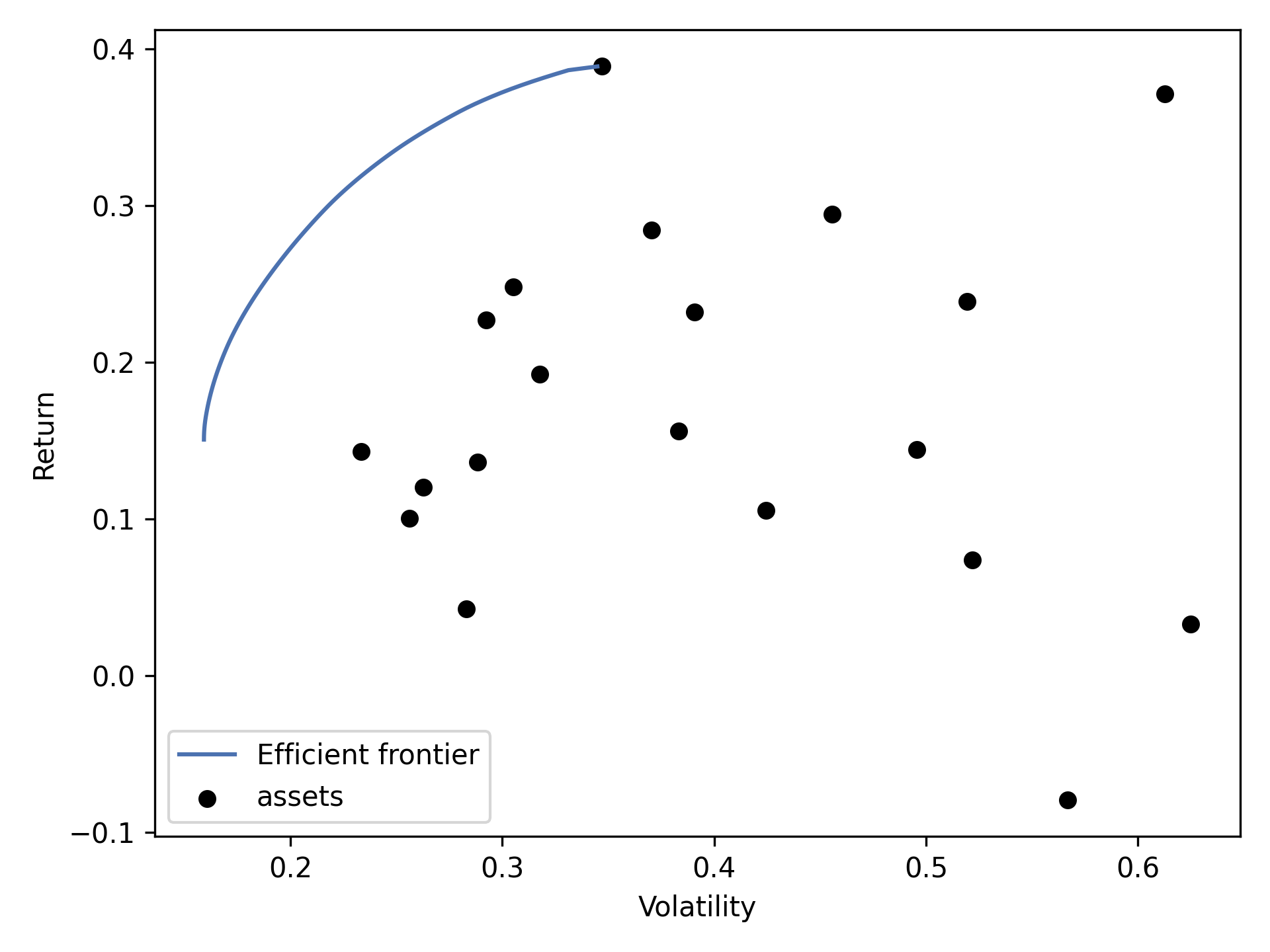](https://pyportfolioopt.readthedocs.io/en/latest/_images/ef_plot.png)
You can explicitly pass a range of parameters (risk, utility, or returns) to generate a frontier:
\# 100 portfolios with risks between 0.10 and 0.30
risk\_range \= np.linspace(0.10, 0.40, 100)
plotting.plot\_efficient\_frontier(ef, ef\_param\="risk", ef\_param\_range\=risk\_range,
show\_assets\=True, showfig\=True)
We can easily generate more complex plots. The following script plots both the efficient frontier and randomly generated (suboptimal) portfolios, coloured by the Sharpe ratio:
fig, ax \= plt.subplots()
ef\_max\_sharpe \= ef.deepcopy()
plotting.plot\_efficient\_frontier(ef, ax\=ax, show\_assets\=False)
\# Find the tangency portfolio
ef\_max\_sharpe.max\_sharpe()
ret\_tangent, std\_tangent, \_ \= ef\_max\_sharpe.portfolio\_performance()
ax.scatter(std\_tangent, ret\_tangent, marker\="\*", s\=100, c\="r", label\="Max Sharpe")
\# Generate random portfolios
n\_samples \= 10000
w \= np.random.dirichlet(np.ones(ef.n\_assets), n\_samples)
rets \= w.dot(ef.expected\_returns)
stds \= np.sqrt(np.diag(w @ ef.cov\_matrix @ w.T))
sharpes \= rets / stds
ax.scatter(stds, rets, marker\=".", c\=sharpes, cmap\="viridis\_r")
\# Output
ax.set\_title("Efficient Frontier with random portfolios")
ax.legend()
plt.tight\_layout()
plt.savefig("ef\_scatter.png", dpi\=200)
plt.show()
This is the result:
> [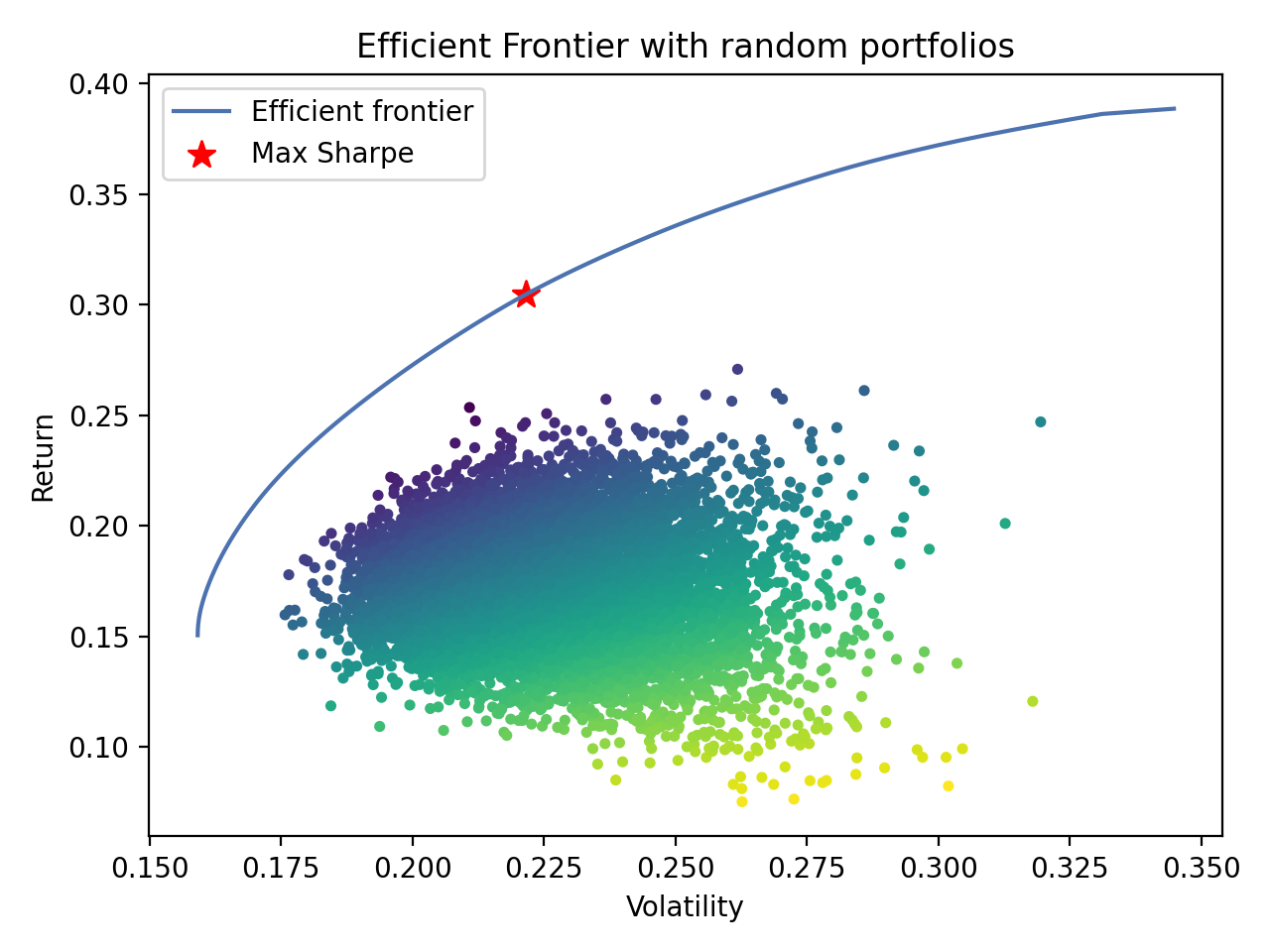](https://pyportfolioopt.readthedocs.io/en/latest/_images/ef_scatter.png)
Documentation reference[¶](https://pyportfolioopt.readthedocs.io/en/latest/Plotting.html#module-pypfopt.plotting "Permalink to this headline")
-----------------------------------------------------------------------------------------------------------------------------------------------
The `plotting` module houses all the functions to generate various plots.
Currently implemented:
> * `plot_covariance` - plot a correlation matrix
> * `plot_dendrogram` - plot the hierarchical clusters in a portfolio
> * `plot_efficient_frontier` – plot the efficient frontier from an EfficientFrontier or CLA object
> * `plot_weights` - bar chart of weights
Tip
To save the plot, pass `filename="somefile.png"` as a keyword argument to any of the plotting functions. This (along with some other kwargs) get passed through [`_plot_io()`](https://pyportfolioopt.readthedocs.io/en/latest/Plotting.html#pypfopt.plotting._plot_io "pypfopt.plotting._plot_io")
before being returned.
`pypfopt.plotting.``_plot_io`(_\*\*kwargs_)[\[source\]](https://pyportfolioopt.readthedocs.io/en/latest/_modules/pypfopt/plotting.html#_plot_io)
[¶](https://pyportfolioopt.readthedocs.io/en/latest/Plotting.html#pypfopt.plotting._plot_io "Permalink to this definition")
Helper method to optionally save the figure to file.
| | |
| --- | --- |
| Parameters: | * **filename** (_str__,_ _optional_) – name of the file to save to, defaults to None (doesn’t save)
* **dpi** (_int_ _(__between 50-500__)_) – dpi of figure to save or plot, defaults to 300
* **showfig** (_bool__,_ _optional_) – whether to plt.show() the figure, defaults to False |
`pypfopt.plotting.``plot_covariance`(_cov\_matrix_, _plot\_correlation=False_, _show\_tickers=True_, _\*\*kwargs_)[\[source\]](https://pyportfolioopt.readthedocs.io/en/latest/_modules/pypfopt/plotting.html#plot_covariance)
[¶](https://pyportfolioopt.readthedocs.io/en/latest/Plotting.html#pypfopt.plotting.plot_covariance "Permalink to this definition")
Generate a basic plot of the covariance (or correlation) matrix, given a covariance matrix.
| | |
| --- | --- |
| Parameters: | * **cov\_matrix** (_pd.DataFrame_ _or_ _np.ndarray_) – covariance matrix
* **plot\_correlation** (_bool__,_ _optional_) – whether to plot the correlation matrix instead, defaults to False.
* **show\_tickers** (_bool__,_ _optional_) – whether to use tickers as labels (not recommended for large portfolios), defaults to True |
| Returns: | matplotlib axis |
| Return type: | matplotlib.axes object |
[](https://pyportfolioopt.readthedocs.io/en/latest/_images/corrplot.png)
`pypfopt.plotting.``plot_dendrogram`(_hrp_, _ax=None_, _show\_tickers=True_, _\*\*kwargs_)[\[source\]](https://pyportfolioopt.readthedocs.io/en/latest/_modules/pypfopt/plotting.html#plot_dendrogram)
[¶](https://pyportfolioopt.readthedocs.io/en/latest/Plotting.html#pypfopt.plotting.plot_dendrogram "Permalink to this definition")
Plot the clusters in the form of a dendrogram.
| | |
| --- | --- |
| Parameters: | * **hrp** (_object_) – HRPpt object that has already been optimized.
* **show\_tickers** (_bool__,_ _optional_) – whether to use tickers as labels (not recommended for large portfolios), defaults to True
* **filename** (_str__,_ _optional_) – name of the file to save to, defaults to None (doesn’t save)
* **showfig** (_bool__,_ _optional_) – whether to plt.show() the figure, defaults to False |
| Returns: | matplotlib axis |
| Return type: | matplotlib.axes object |
[](https://pyportfolioopt.readthedocs.io/en/latest/_images/dendrogram.png)
`pypfopt.plotting.``plot_efficient_frontier`(_opt_, _ef\_param='return'_, _ef\_param\_range=None_, _points=100_, _ax=None_, _show\_assets=True_, _show\_tickers=False_, _\*\*kwargs_)[\[source\]](https://pyportfolioopt.readthedocs.io/en/latest/_modules/pypfopt/plotting.html#plot_efficient_frontier)
[¶](https://pyportfolioopt.readthedocs.io/en/latest/Plotting.html#pypfopt.plotting.plot_efficient_frontier "Permalink to this definition")
Plot the efficient frontier based on either a CLA or EfficientFrontier object.
| | |
| --- | --- |
| Parameters: | * **opt** ([_EfficientFrontier_](https://pyportfolioopt.readthedocs.io/en/latest/MeanVariance.html#pypfopt.efficient_frontier.EfficientFrontier "pypfopt.efficient_frontier.EfficientFrontier")
_or_ [_CLA_](https://pyportfolioopt.readthedocs.io/en/latest/OtherOptimizers.html#pypfopt.cla.CLA "pypfopt.cla.CLA")
) – an instantiated optimizer object BEFORE optimising an objective
* **ef\_param** (_str__,_ _one of {"utility"__,_ _"risk"__,_ _"return"}._) – \[EfficientFrontier\] whether to use a range over utility, risk, or return. Defaults to “return”.
* **ef\_param\_range** (_np.array_ _or_ _list_ _(__recommended to use np.arange_ _or_ _np.linspace__)_) – the range of parameter values for ef\_param. If None, automatically compute a range from min->max return.
* **points** (_int__,_ _optional_) – number of points to plot, defaults to 100. This is overridden if an ef\_param\_range is provided explicitly.
* **show\_assets** (_bool__,_ _optional_) – whether we should plot the asset risks/returns also, defaults to True
* **show\_tickers** (_bool__,_ _optional_) – whether we should annotate each asset with its ticker, defaults to False
* **filename** (_str__,_ _optional_) – name of the file to save to, defaults to None (doesn’t save)
* **showfig** (_bool__,_ _optional_) – whether to plt.show() the figure, defaults to False |
| Returns: | matplotlib axis |
| Return type: | matplotlib.axes object |
[](https://pyportfolioopt.readthedocs.io/en/latest/_images/cla_plot.png)
`pypfopt.plotting.``plot_weights`(_weights_, _ax=None_, _\*\*kwargs_)[\[source\]](https://pyportfolioopt.readthedocs.io/en/latest/_modules/pypfopt/plotting.html#plot_weights)
[¶](https://pyportfolioopt.readthedocs.io/en/latest/Plotting.html#pypfopt.plotting.plot_weights "Permalink to this definition")
Plot the portfolio weights as a horizontal bar chart
| | |
| --- | --- |
| Parameters: | * **weights** (_{ticker: weight} dict_) – the weights outputted by any PyPortfolioOpt optimizer
* **ax** (_matplotlib.axes_) – ax to plot to, optional |
| Returns: | matplotlib axis |
| Return type: | matplotlib.axes |
[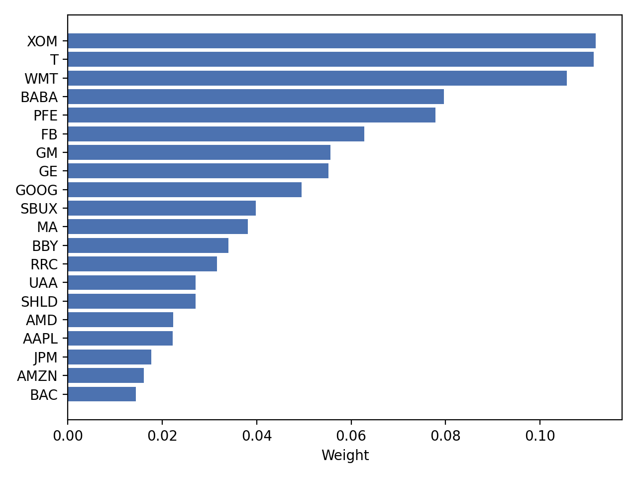](https://pyportfolioopt.readthedocs.io/en/latest/_images/weight_plot.png)
---
# Plotting — PyPortfolioOpt 1.4.1 documentation
* [Docs](https://pyportfolioopt.readthedocs.io/en/stable/index.html)
»
* Plotting
* [Edit on GitHub](https://github.com/robertmartin8/PyPortfolioOpt/blob/1db089602dee348f1eade9b981ca21cd35f1dcca/docs/Plotting.rst)
* * *
Plotting[¶](https://pyportfolioopt.readthedocs.io/en/stable/Plotting.html#plotting "Permalink to this headline")
=================================================================================================================
All of the optimization functions in `EfficientFrontier` produce a single optimal portfolio. However, you may want to plot the entire efficient frontier. This efficient frontier can be thought of in several different ways:
1. The set of all `efficient_risk()` portfolios for a range of target risks
2. The set of all `efficient_return()` portfolios for a range of target returns
3. The set of all `max_quadratic_utility()` portfolios for a range of risk aversions.
The `plotting` module provides support for all three of these approaches. To produce a plot of the efficient frontier, you should instantiate your `EfficientFrontier` object and add constraints like you normally would, but _before_ calling an optimization function (e.g with `ef.max_sharpe()`), you should pass this the instantiated object into `plot.plot_efficient_frontier()`:
ef \= EfficientFrontier(mu, S, weight\_bounds\=(None, None))
ef.add\_constraint(lambda w: w\[0\] \>= 0.2)
ef.add\_constraint(lambda w: w\[2\] \== 0.15)
ef.add\_constraint(lambda w: w\[3\] + w\[4\] <= 0.10)
fig, ax \= plt.subplots()
plotting.plot\_efficient\_frontier(ef, ax\=ax, show\_assets\=True)
plt.show()
This produces the following plot:
> [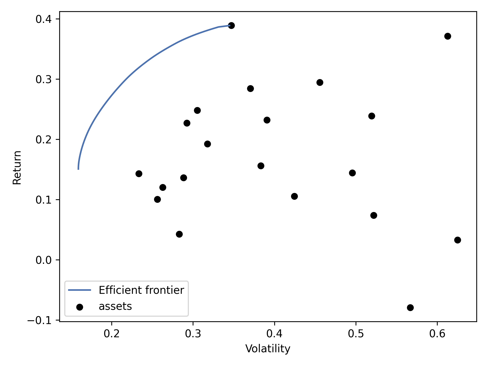](https://pyportfolioopt.readthedocs.io/en/stable/_images/ef_plot.png)
You can explicitly pass a range of parameters (risk, utility, or returns) to generate a frontier:
\# 100 portfolios with risks between 0.10 and 0.30
risk\_range \= np.linspace(0.10, 0.40, 100)
plotting.plot\_efficient\_frontier(ef, ef\_param\="risk", ef\_param\_range\=risk\_range,
show\_assets\=True, showfig\=True)
We can easily generate more complex plots. The following script plots both the efficient frontier and randomly generated (suboptimal) portfolios, coloured by the Sharpe ratio:
fig, ax \= plt.subplots()
plotting.plot\_efficient\_frontier(ef, ax\=ax, show\_assets\=False)
\# Find the tangency portfolio
ef.max\_sharpe()
ret\_tangent, std\_tangent, \_ \= ef.portfolio\_performance()
ax.scatter(std\_tangent, ret\_tangent, marker\="\*", s\=100, c\="r", label\="Max Sharpe")
\# Generate random portfolios
n\_samples \= 10000
w \= np.random.dirichlet(np.ones(len(mu)), n\_samples)
rets \= w.dot(mu)
stds \= np.sqrt(np.diag(w @ S @ w.T))
sharpes \= rets / stds
ax.scatter(stds, rets, marker\=".", c\=sharpes, cmap\="viridis\_r")
\# Output
ax.set\_title("Efficient Frontier with random portfolios")
ax.legend()
plt.tight\_layout()
plt.savefig("ef\_scatter.png", dpi\=200)
plt.show()
This is the result:
> [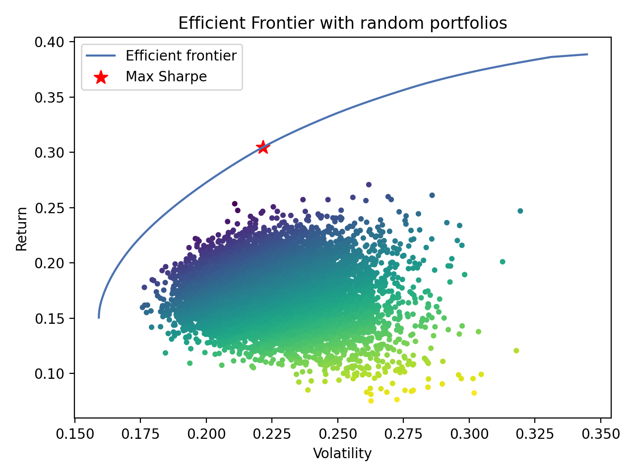](https://pyportfolioopt.readthedocs.io/en/stable/_images/ef_scatter.png)
Documentation reference[¶](https://pyportfolioopt.readthedocs.io/en/stable/Plotting.html#module-pypfopt.plotting "Permalink to this headline")
-----------------------------------------------------------------------------------------------------------------------------------------------
The `plotting` module houses all the functions to generate various plots.
Currently implemented:
> * `plot_covariance` - plot a correlation matrix
> * `plot_dendrogram` - plot the hierarchical clusters in a portfolio
> * `plot_efficient_frontier` – plot the efficient frontier from an EfficientFrontier or CLA object
> * `plot_weights` - bar chart of weights
Tip
To save the plot, pass `filename="somefile.png"` as a keyword argument to any of the plotting functions. This (along with some other kwargs) get passed through [`_plot_io()`](https://pyportfolioopt.readthedocs.io/en/stable/Plotting.html#pypfopt.plotting._plot_io "pypfopt.plotting._plot_io")
before being returned.
`pypfopt.plotting.``_plot_io`(_\*\*kwargs_)[\[source\]](https://pyportfolioopt.readthedocs.io/en/stable/_modules/pypfopt/plotting.html#_plot_io)
[¶](https://pyportfolioopt.readthedocs.io/en/stable/Plotting.html#pypfopt.plotting._plot_io "Permalink to this definition")
Helper method to optionally save the figure to file.
| | |
| --- | --- |
| Parameters: | * **filename** (_str__,_ _optional_) – name of the file to save to, defaults to None (doesn’t save)
* **dpi** (_int_ _(__between 50-500__)_) – dpi of figure to save or plot, defaults to 300
* **showfig** (_bool__,_ _optional_) – whether to plt.show() the figure, defaults to False |
`pypfopt.plotting.``plot_covariance`(_cov\_matrix_, _plot\_correlation=False_, _show\_tickers=True_, _\*\*kwargs_)[\[source\]](https://pyportfolioopt.readthedocs.io/en/stable/_modules/pypfopt/plotting.html#plot_covariance)
[¶](https://pyportfolioopt.readthedocs.io/en/stable/Plotting.html#pypfopt.plotting.plot_covariance "Permalink to this definition")
Generate a basic plot of the covariance (or correlation) matrix, given a covariance matrix.
| | |
| --- | --- |
| Parameters: | * **cov\_matrix** (_pd.DataFrame_ _or_ _np.ndarray_) – covariance matrix
* **plot\_correlation** (_bool__,_ _optional_) – whether to plot the correlation matrix instead, defaults to False.
* **show\_tickers** (_bool__,_ _optional_) – whether to use tickers as labels (not recommended for large portfolios), defaults to True |
| Returns: | matplotlib axis |
| Return type: | matplotlib.axes object |
[](https://pyportfolioopt.readthedocs.io/en/stable/_images/corrplot.png)
`pypfopt.plotting.``plot_dendrogram`(_hrp_, _ax=None_, _show\_tickers=True_, _\*\*kwargs_)[\[source\]](https://pyportfolioopt.readthedocs.io/en/stable/_modules/pypfopt/plotting.html#plot_dendrogram)
[¶](https://pyportfolioopt.readthedocs.io/en/stable/Plotting.html#pypfopt.plotting.plot_dendrogram "Permalink to this definition")
Plot the clusters in the form of a dendrogram.
| | |
| --- | --- |
| Parameters: | * **hrp** (_object_) – HRPpt object that has already been optimized.
* **show\_tickers** (_bool__,_ _optional_) – whether to use tickers as labels (not recommended for large portfolios), defaults to True
* **filename** (_str__,_ _optional_) – name of the file to save to, defaults to None (doesn’t save)
* **showfig** (_bool__,_ _optional_) – whether to plt.show() the figure, defaults to False |
| Returns: | matplotlib axis |
| Return type: | matplotlib.axes object |
[](https://pyportfolioopt.readthedocs.io/en/stable/_images/dendrogram.png)
`pypfopt.plotting.``plot_efficient_frontier`(_opt_, _ef\_param='return'_, _ef\_param\_range=None_, _points=100_, _ax=None_, _show\_assets=True_, _\*\*kwargs_)[\[source\]](https://pyportfolioopt.readthedocs.io/en/stable/_modules/pypfopt/plotting.html#plot_efficient_frontier)
[¶](https://pyportfolioopt.readthedocs.io/en/stable/Plotting.html#pypfopt.plotting.plot_efficient_frontier "Permalink to this definition")
Plot the efficient frontier based on either a CLA or EfficientFrontier object.
| | |
| --- | --- |
| Parameters: | * **opt** ([_EfficientFrontier_](https://pyportfolioopt.readthedocs.io/en/stable/MeanVariance.html#pypfopt.efficient_frontier.EfficientFrontier "pypfopt.efficient_frontier.EfficientFrontier")
_or_ [_CLA_](https://pyportfolioopt.readthedocs.io/en/stable/OtherOptimizers.html#pypfopt.cla.CLA "pypfopt.cla.CLA")
) – an instantiated optimizer object BEFORE optimising an objective
* **ef\_param** (_str__,_ _one of {"utility"__,_ _"risk"__,_ _"return"}._) – \[EfficientFrontier\] whether to use a range over utility, risk, or return. Defaults to “return”.
* **ef\_param\_range** (_np.array_ _or_ _list_ _(__recommended to use np.arange_ _or_ _np.linspace__)_) – the range of parameter values for ef\_param. If None, automatically compute a range from min->max return.
* **points** (_int__,_ _optional_) – number of points to plot, defaults to 100. This is overridden if an ef\_param\_range is provided explicitly.
* **show\_assets** (_bool__,_ _optional_) – whether we should plot the asset risks/returns also, defaults to True
* **filename** (_str__,_ _optional_) – name of the file to save to, defaults to None (doesn’t save)
* **showfig** (_bool__,_ _optional_) – whether to plt.show() the figure, defaults to False |
| Returns: | matplotlib axis |
| Return type: | matplotlib.axes object |
[](https://pyportfolioopt.readthedocs.io/en/stable/_images/cla_plot.png)
`pypfopt.plotting.``plot_weights`(_weights_, _ax=None_, _\*\*kwargs_)[\[source\]](https://pyportfolioopt.readthedocs.io/en/stable/_modules/pypfopt/plotting.html#plot_weights)
[¶](https://pyportfolioopt.readthedocs.io/en/stable/Plotting.html#pypfopt.plotting.plot_weights "Permalink to this definition")
Plot the portfolio weights as a horizontal bar chart
| | |
| --- | --- |
| Parameters: | * **weights** (_{ticker: weight} dict_) – the weights outputted by any PyPortfolioOpt optimizer
* **ax** (_matplotlib.axes_) – ax to plot to, optional |
| Returns: | matplotlib axis |
| Return type: | matplotlib.axes |
[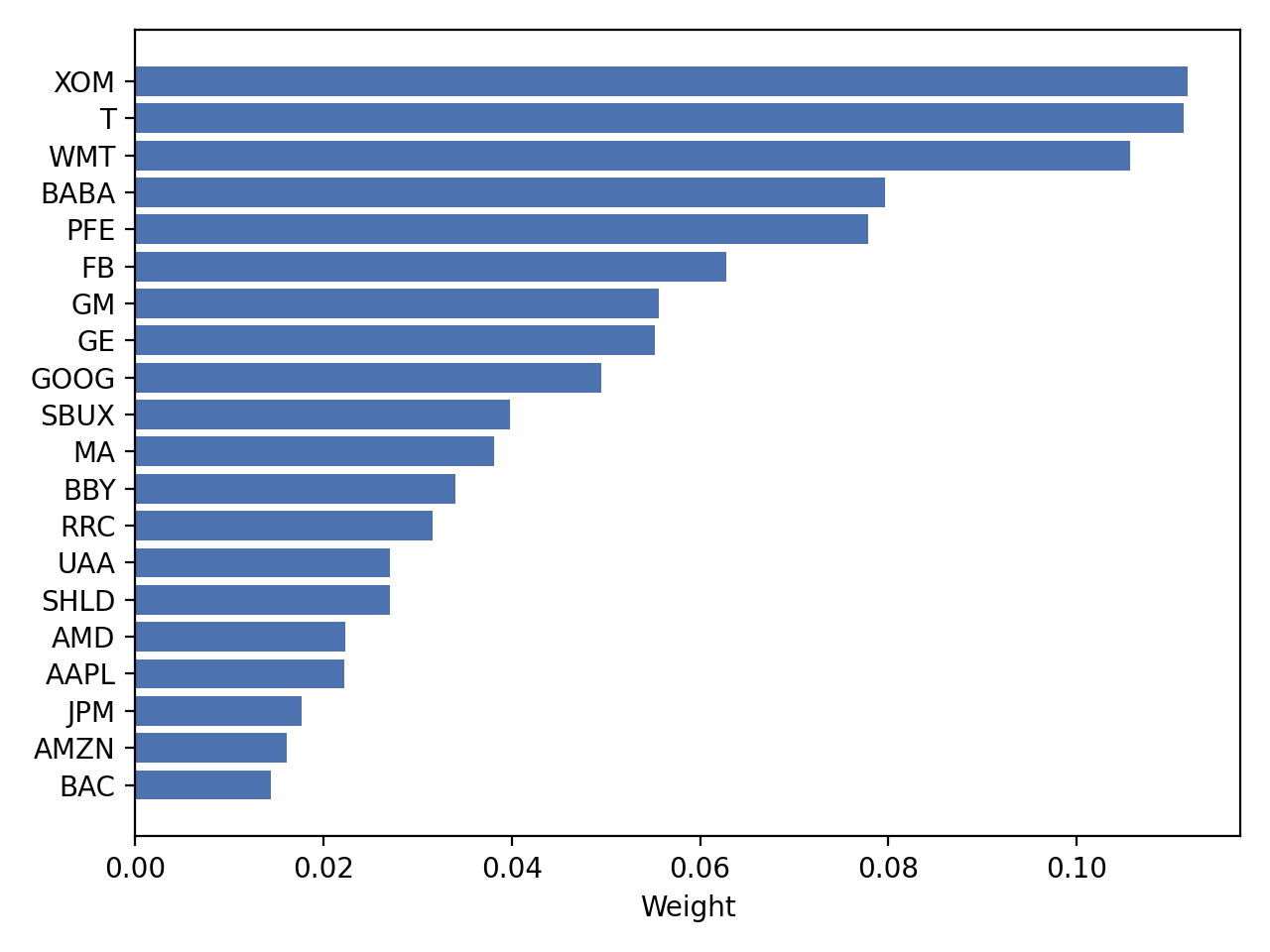](https://pyportfolioopt.readthedocs.io/en/stable/_images/weight_plot.png)
---
# Roadmap and Changelog — PyPortfolioOpt 1.4.1 documentation
* [Docs](https://pyportfolioopt.readthedocs.io/en/stable/index.html)
»
* Roadmap and Changelog
* [Edit on GitHub](https://github.com/robertmartin8/PyPortfolioOpt/blob/1db089602dee348f1eade9b981ca21cd35f1dcca/docs/Roadmap.rst)
* * *
Roadmap and Changelog[¶](https://pyportfolioopt.readthedocs.io/en/stable/Roadmap.html#roadmap-and-changelog "Permalink to this headline")
==========================================================================================================================================
Roadmap[¶](https://pyportfolioopt.readthedocs.io/en/stable/Roadmap.html#id1 "Permalink to this headline")
----------------------------------------------------------------------------------------------------------
These are some of the features that I think would greatly improve PyPortfolioOpt; if you are interested in implementing one of these, raise an issue or send me an email and we can discuss. If you have any other feature requests, please raise them using GitHub [issues](https://github.com/robertmartin8/PyPortfolioOpt/issues)
* Open-source backtests using either [Backtrader](https://www.backtrader.com/)
or [Zipline](https://github.com/quantopian/zipline)
.
* Risk parity
* Optimising for higher moments (i.e skew and kurtosis)
* Factor modelling - this is conceptually doable, but a lot of thought needs to be put into the API.
* Monte Carlo optimization with custom distributions
* Further support for different risk/return models
1.4.0[¶](https://pyportfolioopt.readthedocs.io/en/stable/Roadmap.html#id2 "Permalink to this headline")
--------------------------------------------------------------------------------------------------------
* Finally implemented CVaR optimization! This has been one of the most requested features. Many thanks to [Nicolas Knudde](https://github.com/nknudde)
for the initial draft.
* Re-architected plotting so users can pass an ax, allowing for complex plots (see cookbook).
* Helper method to compute the max-return portfolio (thanks to [Philipp Schiele](https://github.com/phschiele)
) for the suggestion).
* Several bug fixes and test improvements (thanks to [Carl Peasnell](https://github.com/SeaPea1)
).
### 1.4.1[¶](https://pyportfolioopt.readthedocs.io/en/stable/Roadmap.html#id3 "Permalink to this headline")
* 100% test coverage
* Reorganised docs; added FAQ page
* Reorganised module structure to make it more scalable
* Python 3.9 support, dockerfile versioning, misc packaging improvements (e.g cvxopt optional)
1.3.0[¶](https://pyportfolioopt.readthedocs.io/en/stable/Roadmap.html#id4 "Permalink to this headline")
--------------------------------------------------------------------------------------------------------
* Significantly improved plotting functionality: can now plot constrained efficient frontier!
* Efficient semivariance portfolios (thanks to [Philipp Schiele](https://github.com/phschiele)
)
* Improved functionality for portfolios with short positions (thanks to [Rich Caputo](https://github.com/arcaputo3)
).
* Significant improvement in test coverage (thanks to [Carl Peasnell](https://github.com/SeaPea1)
).
* Several bug fixes and usability improvements.
* Migrated from TravisCI to Github Actions.
### 1.3.1[¶](https://pyportfolioopt.readthedocs.io/en/stable/Roadmap.html#id7 "Permalink to this headline")
* Minor cleanup (forgotten commits from v1.3.0).
1.2.0[¶](https://pyportfolioopt.readthedocs.io/en/stable/Roadmap.html#id8 "Permalink to this headline")
--------------------------------------------------------------------------------------------------------
* Added Idzorek’s method for calculating the `omega` matrix given percentage confidences.
* Fixed max sharpe to allow for custom constraints
* Grouped sector constraints
* Improved error tracebacks
* Adding new cookbook for examples (in progress).
* Packaging: added bettter instructions for windows, added docker support.
### 1.2.1[¶](https://pyportfolioopt.readthedocs.io/en/stable/Roadmap.html#id9 "Permalink to this headline")
Fixed critical ordering bug in sector constraints
### 1.2.2[¶](https://pyportfolioopt.readthedocs.io/en/stable/Roadmap.html#id10 "Permalink to this headline")
Matplotlib now required dependency; support for pandas 1.0.
### 1.2.3[¶](https://pyportfolioopt.readthedocs.io/en/stable/Roadmap.html#id11 "Permalink to this headline")
* Added support for changing solvers and verbose output
* Changed dict to OrderedDict to support python 3.5
* Improved packaging/dependencies: simplified requirements.txt, improved processes before pushing.
### 1.2.4[¶](https://pyportfolioopt.readthedocs.io/en/stable/Roadmap.html#id12 "Permalink to this headline")
* Fixed bug in Ledoit-Wolf shrinkage calculation.
* Fixed bug in plotting docs that caused them not to render.
### 1.2.5[¶](https://pyportfolioopt.readthedocs.io/en/stable/Roadmap.html#id13 "Permalink to this headline")
* Fixed compounding in `expected_returns` (thanks to [Aditya Bhutra](https://github.com/bhutraaditya)
).
* Improvements in advanced cvxpy API (thanks to [Pat Newell](https://github.com/pmn4)
).
* Deprecating James-Stein
* Exposed `linkage_method` in HRP.
* Added support for cvxpy 1.1.
* Added an error check for `efficient_risk`.
* Small improvements to docs.
### 1.2.6[¶](https://pyportfolioopt.readthedocs.io/en/stable/Roadmap.html#id14 "Permalink to this headline")
* Fixed order-dependence bug in Black-Litterman `market_implied_prior_returns`
* Fixed inaccuracy in BL cookbook.
* Fixed bug in exponential covariance.
### 1.2.7[¶](https://pyportfolioopt.readthedocs.io/en/stable/Roadmap.html#id15 "Permalink to this headline")
* Fixed bug which required conservative risk targets for long/short portfolios.
1.1.0[¶](https://pyportfolioopt.readthedocs.io/en/stable/Roadmap.html#id16 "Permalink to this headline")
---------------------------------------------------------------------------------------------------------
* Multiple additions and improvements to `risk_models`:
* Introduced a new API, in which the function `risk_models.risk_matrix(method="...")` allows all the different risk models to be called. This should make testing easier.
* All methods now accept returns data instead of prices, if you set the flag `returns_data=True`.
* Automatically fix non-positive semidefinite covariance matrices!
* Additions and improvements to `expected_returns`:
* Introduced a new API, in which the function `expected_returns.return_model(method="...")` allows all the different return models to be called. This should make testing easier.
* Added option to ‘properly’ compound returns.
* Added the CAPM return model.
* `from pypfopt import plotting`: moved all plotting functionality into a new class and added new plots. All other plotting functions (scattered in different classes) have been retained, but are now deprecated.
1.0.0[¶](https://pyportfolioopt.readthedocs.io/en/stable/Roadmap.html#id17 "Permalink to this headline")
---------------------------------------------------------------------------------------------------------
* Migrated backend from `scipy` to `cvxpy` and made significant breaking changes to the API
* PyPortfolioOpt is now significantly more robust and numerically stable.
* These changes will not affect basic users, who can still access features like `max_sharpe()`.
* However, additional objectives and constraints (including L2 regularisation) are now explicitly added before optimising some ‘primary’ objective.
* Added basic plotting capabilities for the efficient frontier, hierarchical clusters, and HRP dendrograms.
* Added a basic transaction cost objective.
* Made breaking changes to some modules and classes so that PyPortfolioOpt is easier to extend in future:
* Replaced `BaseScipyOptimizer` with `BaseConvexOptimizer`
* `hierarchical_risk_parity` was replaced by `hierarchical_portfolios` to leave the door open for other hierarchical methods.
* Sadly, removed CVaR optimization for the time being until I can properly fix it.
### 1.0.1[¶](https://pyportfolioopt.readthedocs.io/en/stable/Roadmap.html#id18 "Permalink to this headline")
Fixed minor issues in CLA: weight bound bug, `efficient_frontier` needed weights to be called, `set_weights` not needed.
### 1.0.2[¶](https://pyportfolioopt.readthedocs.io/en/stable/Roadmap.html#id19 "Permalink to this headline")
Fixed small but important bug where passing `expected_returns=None` fails. According to the docs, users should be able to only pass covariance if they want to only optimize min volatility.
0.5.0[¶](https://pyportfolioopt.readthedocs.io/en/stable/Roadmap.html#id20 "Permalink to this headline")
---------------------------------------------------------------------------------------------------------
* Black-Litterman model and docs.
* Custom bounds per asset
* Improved `BaseOptimizer`, adding a method that writes weights to text and fixing a bug in `set_weights`.
* Unconstrained quadratic utility optimization (analytic)
* Revamped docs, with information on types of attributes and more examples.
### 0.5.1[¶](https://pyportfolioopt.readthedocs.io/en/stable/Roadmap.html#id21 "Permalink to this headline")
Fixed an error with dot products by amending the pandas requirements.
### 0.5.2[¶](https://pyportfolioopt.readthedocs.io/en/stable/Roadmap.html#id22 "Permalink to this headline")
Made PuLP, sklearn, noisyopt optional dependencies to improve installation experience.
### 0.5.3[¶](https://pyportfolioopt.readthedocs.io/en/stable/Roadmap.html#id23 "Permalink to this headline")
* Fixed an optimization bug in `EfficientFrontier.efficient_risk`. An error is now thrown if optimization fails.
* Added a hidden API to change the scipy optimizer method.
### 0.5.4[¶](https://pyportfolioopt.readthedocs.io/en/stable/Roadmap.html#id24 "Permalink to this headline")
* Improved the Black-Litterman linear algebra to avoid inverting the uncertainty matrix. It is now possible to have 100% confidence in views.
* Clarified regarding the role of tau.
* Added a `pipfile` for `pipenv` users.
* Removed Value-at-risk from docs to discourage usage until it is properly fixed.
### 0.5.5[¶](https://pyportfolioopt.readthedocs.io/en/stable/Roadmap.html#id25 "Permalink to this headline")
Began migration to cvxpy by changing the discrete allocation backend from PuLP to cvxpy.
0.4.0[¶](https://pyportfolioopt.readthedocs.io/en/stable/Roadmap.html#id26 "Permalink to this headline")
---------------------------------------------------------------------------------------------------------
* Major improvements to `discrete_allocation`. Added functionality to allocate shorts; modified the linear programming method suggested by [Dingyuan Wang](https://github.com/gumblex)
; added postprocessing section to User Guide.
* Further refactoring and docs for `HRPOpt`.
* Major documentation update, e.g to support custom optimizers
### 0.4.1[¶](https://pyportfolioopt.readthedocs.io/en/stable/Roadmap.html#id27 "Permalink to this headline")
* Added CLA back in after getting permission from Dr Marcos López de Prado
* Added more tests for different risk models.
### 0.4.2[¶](https://pyportfolioopt.readthedocs.io/en/stable/Roadmap.html#id28 "Permalink to this headline")
* Minor fix for `clean_weights`
* Removed official support for python 3.4.
* Minor improvement to semicovariance, thanks to [Felipe Schneider](https://github.com/schneiderfelipe)
.
### 0.4.3[¶](https://pyportfolioopt.readthedocs.io/en/stable/Roadmap.html#id29 "Permalink to this headline")
* Added `prices_from_returns` utility function and provided better docs for `returns_from_prices`.
* Added `cov_to_corr` method to produce correlation matrices from covariance matrices.
* Fixed readme examples.
0.3.0[¶](https://pyportfolioopt.readthedocs.io/en/stable/Roadmap.html#id30 "Permalink to this headline")
---------------------------------------------------------------------------------------------------------
* Merged an amazing PR from [Dingyuan Wang](https://github.com/gumblex)
that rearchitects the project to make it more self-consistent and extensible.
* New algorithm: ML de Prado’s CLA
* New algorithms for converting continuous allocation to discrete (using linear programming).
* Merged a [PR](https://github.com/robertmartin8/PyPortfolioOpt/pull/22)
implementing Single Factor and Constant Correlation shrinkage.
### 0.3.1[¶](https://pyportfolioopt.readthedocs.io/en/stable/Roadmap.html#id32 "Permalink to this headline")
Merged [PR](https://github.com/robertmartin8/PyPortfolioOpt/pull/23)
from [TommyBark](https://github.com/TommyBark)
fixing a bug in the arguments of a call to `portfolio_performance`.
### 0.3.3[¶](https://pyportfolioopt.readthedocs.io/en/stable/Roadmap.html#id33 "Permalink to this headline")
Migrated the project internally to use the `poetry` dependency manager. Will still keep `setup.py` and `requirements.txt`, but `poetry` is now the recommended way to interact with PyPortfolioOpt.
### 0.3.4[¶](https://pyportfolioopt.readthedocs.io/en/stable/Roadmap.html#id34 "Permalink to this headline")
Refactored shrinkage models, including single factor and constant correlation.
0.2.0[¶](https://pyportfolioopt.readthedocs.io/en/stable/Roadmap.html#id35 "Permalink to this headline")
---------------------------------------------------------------------------------------------------------
* Hierarchical Risk Parity optimization
* Semicovariance matrix
* Exponential covariance matrix
* CVaR optimization
* Better support for custom objective functions
* Multiple bug fixes (including minimum volatility vs minimum variance)
* Refactored so all optimizers inherit from a `BaseOptimizer`.
### 0.2.1[¶](https://pyportfolioopt.readthedocs.io/en/stable/Roadmap.html#id36 "Permalink to this headline")
* Included python 3.7 in travis build
* Merged PR from [schneiderfelipe](https://github.com/schneiderfelipe)
to fix an error message.
0.1.0[¶](https://pyportfolioopt.readthedocs.io/en/stable/Roadmap.html#id37 "Permalink to this headline")
---------------------------------------------------------------------------------------------------------
Initial release:
* Efficient frontier (max sharpe, min variance, target risk/return)
* L2 regularisation
* Discrete allocation
* Mean historical returns, exponential mean returns
* Sample covariance, sklearn wrappers.
* Tests
* Docs
### 0.1.1[¶](https://pyportfolioopt.readthedocs.io/en/stable/Roadmap.html#id38 "Permalink to this headline")
Minor bug fixes and documentation
---
# FAQs — PyPortfolioOpt 1.5.4 documentation
* [Docs](https://pyportfolioopt.readthedocs.io/en/latest/index.html)
»
* FAQs
* [Edit on GitHub](https://github.com/robertmartin8/PyPortfolioOpt/blob/master/docs/FAQ.rst)
* * *
FAQs[¶](https://pyportfolioopt.readthedocs.io/en/latest/FAQ.html#faqs "Permalink to this headline")
====================================================================================================
Constraining a score[¶](https://pyportfolioopt.readthedocs.io/en/latest/FAQ.html#constraining-a-score "Permalink to this headline")
------------------------------------------------------------------------------------------------------------------------------------
Suppose that for each asset you have some “score” – it could be an ESG metric, or some custom risk/return metric. It is simple to specify linear constraints, like “portfolio ESG score must be greater than x”: you simply create a vector of scores, add a constraint on the dot product of those scores with the portfolio weights, then optimize your objective:
esg\_scores \= \[0.3, 0.1, 0.4, 0.1, 0.5, 0.9, 0.2\]
portfolio\_min\_score \= 0.5
ef \= EfficientFrontier(mu, S)
ef.add\_constraint(lambda w: esg\_scores @ w \>= portfolio\_min\_score)
ef.min\_volatility()
Constraining the number of assets[¶](https://pyportfolioopt.readthedocs.io/en/latest/FAQ.html#constraining-the-number-of-assets "Permalink to this headline")
--------------------------------------------------------------------------------------------------------------------------------------------------------------
Unfortunately, cardinality constraints are not convex, making them difficult to implement.
However, we can treat it as a mixed-integer program and solve (provided you have access to a solver). for small problems with less than 1000 variables and constraints, you can use the community version of CPLEX: `pip install cplex`. In the below example, we limit the portfolio to at most 10 assets:
import cvxpy as cp
ef \= EfficientFrontier(mu, S, solver\=cp.CPLEX)
booleans \= cp.Variable(len(ef.tickers), boolean\=True)
ef.add\_constraint(lambda x: x <= booleans)
ef.add\_constraint(lambda x: cp.sum(booleans) <= 10)
ef.min\_volatility()
This does not play well with `max_sharpe`, and needs to be modified for different bounds. See [this issue](https://github.com/robertmartin8/PyPortfolioOpt/issues/243)
for further discussion.
Tracking error[¶](https://pyportfolioopt.readthedocs.io/en/latest/FAQ.html#tracking-error "Permalink to this headline")
------------------------------------------------------------------------------------------------------------------------
Tracking error can either be used as an objective (as described in [General Efficient Frontier](https://pyportfolioopt.readthedocs.io/en/latest/GeneralEfficientFrontier.html#efficient-frontier)
) or as a constraint. This is an example of adding a tracking error constraint:
from objective functions import ex\_ante\_tracking\_error
benchmark\_weights \= ... \# benchmark
ef \= EfficientFrontier(mu, S)
ef.add\_constraint(ex\_ante\_tracking\_error, cov\_matrix\=ef.cov\_matrix,
benchmark\_weights\=benchmark\_weights)
ef.min\_volatility()
---
# FAQs — PyPortfolioOpt 1.4.1 documentation
* [Docs](https://pyportfolioopt.readthedocs.io/en/stable/index.html)
»
* FAQs
* [Edit on GitHub](https://github.com/robertmartin8/PyPortfolioOpt/blob/1db089602dee348f1eade9b981ca21cd35f1dcca/docs/FAQ.rst)
* * *
FAQs[¶](https://pyportfolioopt.readthedocs.io/en/stable/FAQ.html#faqs "Permalink to this headline")
====================================================================================================
Constraining the number of assets[¶](https://pyportfolioopt.readthedocs.io/en/stable/FAQ.html#constraining-the-number-of-assets "Permalink to this headline")
--------------------------------------------------------------------------------------------------------------------------------------------------------------
Unfortunately, cardinality constraints are not convex, making them difficult to implement.
However, we can treat it as a mixed-integer program and solve (provided you have access to a solver). for small problems with less than 1000 variables and constraints, you can use the community version of CPLEX: `pip install cplex`. In the below example, we limit the portfolio to at most 10 assets:
ef \= EfficientFrontier(mu, S, solver\=cp.CPLEX)
booleans \= cp.Variable(len(ef.tickers), boolean\=True)
ef.add\_constraint(lambda x: x <= booleans)
ef.add\_constraint(lambda x: cp.sum(booleans) <= 10)
ef.min\_volatility()
This does not play well with `max_sharpe`, and needs to be modified for different bounds. See [this issue](https://github.com/robertmartin8/PyPortfolioOpt/issues/243)
for further discussion.
Tracking error[¶](https://pyportfolioopt.readthedocs.io/en/stable/FAQ.html#tracking-error "Permalink to this headline")
------------------------------------------------------------------------------------------------------------------------
Tracking error can either be used as an objective (as described in [General Efficient Frontier](https://pyportfolioopt.readthedocs.io/en/stable/GeneralEfficientFrontier.html#efficient-frontier)
) or as a constraint. This is an example of adding a tracking error constraint:
from objective functions import ex\_ante\_tracking\_error
benchmark\_weights \= ... \# benchmark
ef \= EfficientFrontier(mu, S)
ef.add\_constraint(ex\_ante\_tracking\_error, cov\_matrix\=ef.cov\_matrix,
benchmark\_weights\=benchmark\_weights)
ef.min\_volatility()
---
# Contributing — PyPortfolioOpt 1.4.1 documentation
* [Docs](https://pyportfolioopt.readthedocs.io/en/stable/index.html)
»
* Contributing
* [Edit on GitHub](https://github.com/robertmartin8/PyPortfolioOpt/blob/1db089602dee348f1eade9b981ca21cd35f1dcca/docs/Contributing.rst)
* * *
Contributing[¶](https://pyportfolioopt.readthedocs.io/en/stable/Contributing.html#contributing "Permalink to this headline")
=============================================================================================================================
Some of the things that I’d love for people to help with:
* Improve performance of existing code (but not at the cost of readability)
* Add new optimization objectives. For example, if you would like to use something other than the Sharpe ratio, write an optimizer! (or suggest it in [Issues](https://github.com/robertmartin8/PyPortfolioOpt/issues)
and I will have a go).
* Help me write more tests! If you are someone learning about quant finance and/or unit testing in python, what better way to practice than to write some tests on an open-source project! Feel free to check for edge cases, or for uncommon parameter combinations which may cause silent errors.
Guidelines[¶](https://pyportfolioopt.readthedocs.io/en/stable/Contributing.html#guidelines "Permalink to this headline")
-------------------------------------------------------------------------------------------------------------------------
### Seek early feedback[¶](https://pyportfolioopt.readthedocs.io/en/stable/Contributing.html#seek-early-feedback "Permalink to this headline")
Before you start coding your contribution, it may be wise to [raise an issue](https://github.com/robertmartin8/PyPortfolioOpt/issues)
on GitHub to discuss whether the contribution is appropriate for the project.
### Code style[¶](https://pyportfolioopt.readthedocs.io/en/stable/Contributing.html#code-style "Permalink to this headline")
For this project I have used [Black](https://github.com/ambv/black)
as the formatting standard, with all of the default settings. It would be much appreciated if any PRs follow this standard because if not I will have to format before merging.
### Testing[¶](https://pyportfolioopt.readthedocs.io/en/stable/Contributing.html#testing "Permalink to this headline")
Any contributions **must** be accompanied by unit tests (written with `pytest`). These are incredibly simple to write, just find the relevant test file (or create a new one), and write a bunch of `assert` statements. The test should be applied to the dummy dataset I have provided in `tests/stock_prices.csv`, and should cover core functionality, warnings/errors (check that they are raised as expected), and limiting behaviour or edge cases.
### Documentation[¶](https://pyportfolioopt.readthedocs.io/en/stable/Contributing.html#documentation "Permalink to this headline")
Inline comments are great when needed, but don’t go overboard. Docstring content should follow [PEP257](https://stackoverflow.com/questions/2557110/what-to-put-in-a-python-module-docstring)
semantically and sphinx syntactically, such that sphinx can automatically document the methods and their arguments. I am personally not a fan of writing long paragraphs in the docstrings: in my view, docstrings should state briefly how an object can be used, while the rest of the explanation and theoretical background should be offloaded to ReadTheDocs.
I would appreciate if changes are accompanied by relevant documentation - it doesn’t have to be pretty, because I will probably try to tidy it up before it goes onto ReadTheDocs, but it’d make things a lot simpler to have the person who wrote the code explain it in their own words.
Questions[¶](https://pyportfolioopt.readthedocs.io/en/stable/Contributing.html#questions "Permalink to this headline")
-----------------------------------------------------------------------------------------------------------------------
If you have any questions related to the project, it is probably best to [raise an issue](https://github.com/robertmartin8/PyPortfolioOpt/issues)
and I will tag it as a question.
If you have questions _unrelated_ to the project, drop me an email - contact details can be found on my [website](https://reasonabledeviations.com/about/)
.
Bugs/issues[¶](https://pyportfolioopt.readthedocs.io/en/stable/Contributing.html#bugs-issues "Permalink to this headline")
---------------------------------------------------------------------------------------------------------------------------
If you find any bugs or the portfolio optimization is not working as expected, feel free to [raise an issue](https://github.com/robertmartin8/PyPortfolioOpt/issues)
. I would ask that you provide the following information in the issue:
* Descriptive title so that other users can see the existing issues
* Operating system, python version, and python distribution (optional).
* Minimal example for reproducing the issue.
* What you expected to happen
* What actually happened
* A full traceback of the error message (omit personal details as you see fit).
---
# Roadmap and Changelog — PyPortfolioOpt 1.5.4 documentation
* [Docs](https://pyportfolioopt.readthedocs.io/en/latest/index.html)
»
* Roadmap and Changelog
* [Edit on GitHub](https://github.com/robertmartin8/PyPortfolioOpt/blob/master/docs/Roadmap.rst)
* * *
Roadmap and Changelog[¶](https://pyportfolioopt.readthedocs.io/en/latest/Roadmap.html#roadmap-and-changelog "Permalink to this headline")
==========================================================================================================================================
Roadmap[¶](https://pyportfolioopt.readthedocs.io/en/latest/Roadmap.html#id1 "Permalink to this headline")
----------------------------------------------------------------------------------------------------------
PyPortfolioOpt is now a “mature” package – it is stable and I don’t intend to implement major new functionality (though I will endeavour to fix bugs).
1.5.0[¶](https://pyportfolioopt.readthedocs.io/en/latest/Roadmap.html#id2 "Permalink to this headline")
--------------------------------------------------------------------------------------------------------
* Major redesign of the backend, thanks to [Philipp Schiele](https://github.com/phschiele)
- Becuase we use `cp.Parameter`, we can efficiently re-run optimisation problems with different constants (e.g risk targets) - This leads to a significant improvement in plotting performance as we no longer have to repeatedly re-instantiate `EfficientFrontier`.
* Several misc bug fixes (thanks to [Eric Armbruster](https://github.com/armbruer)
and [Ayoub Ennassiri](https://github.com/samatix)
)
### 1.5.1[¶](https://pyportfolioopt.readthedocs.io/en/latest/Roadmap.html#id3 "Permalink to this headline")
Mucked up the versioning on the 1.5.0 launch. Sorry!
### 1.5.2[¶](https://pyportfolioopt.readthedocs.io/en/latest/Roadmap.html#id4 "Permalink to this headline")
Minor bug fixes
### 1.5.3[¶](https://pyportfolioopt.readthedocs.io/en/latest/Roadmap.html#id5 "Permalink to this headline")
* Reworked packaging: `cvxpy` is no longer a requirement as we default to `ECOS_BB` for discrete allocation.
* Bumped minimum python version to `3.8`. I would love to keep as many versions compatible (and I think most of the functionality _should_ still work with `3.6, 3.7` but the dependencies have gotten too tricky to manage).
* Changed to numpy pseudoinverse to allow for “cash” assets
* Ticker labels for efficient frontier plot
### 1.5.4[¶](https://pyportfolioopt.readthedocs.io/en/latest/Roadmap.html#id6 "Permalink to this headline")
* Fixed `cvxpy` deprecating deepcopy. Thanks to Philipp for the fix!
* Several other tiny checks and bug fixes. Cheers to everyone for the PRs!
1.4.0[¶](https://pyportfolioopt.readthedocs.io/en/latest/Roadmap.html#id7 "Permalink to this headline")
--------------------------------------------------------------------------------------------------------
* Finally implemented CVaR optimization! This has been one of the most requested features. Many thanks to [Nicolas Knudde](https://github.com/nknudde)
for the initial draft.
* Re-architected plotting so users can pass an ax, allowing for complex plots (see cookbook).
* Helper method to compute the max-return portfolio (thanks to [Philipp Schiele](https://github.com/phschiele)
) for the suggestion).
* Several bug fixes and test improvements (thanks to [Carl Peasnell](https://github.com/SeaPea1)
).
### 1.4.1[¶](https://pyportfolioopt.readthedocs.io/en/latest/Roadmap.html#id9 "Permalink to this headline")
* 100% test coverage
* Reorganised docs; added FAQ page
* Reorganised module structure to make it more scalable
* Python 3.9 support, dockerfile versioning, misc packaging improvements (e.g cvxopt optional)
### 1.4.2[¶](https://pyportfolioopt.readthedocs.io/en/latest/Roadmap.html#id10 "Permalink to this headline")
* Implemented CDaR optimization – full credit to [Nicolas Knudde](https://github.com/nknudde)
.
* Misc bug fixes
1.3.0[¶](https://pyportfolioopt.readthedocs.io/en/latest/Roadmap.html#id12 "Permalink to this headline")
---------------------------------------------------------------------------------------------------------
* Significantly improved plotting functionality: can now plot constrained efficient frontier!
* Efficient semivariance portfolios (thanks to [Philipp Schiele](https://github.com/phschiele)
)
* Improved functionality for portfolios with short positions (thanks to [Rich Caputo](https://github.com/arcaputo3)
).
* Significant improvement in test coverage (thanks to [Carl Peasnell](https://github.com/SeaPea1)
).
* Several bug fixes and usability improvements.
* Migrated from TravisCI to Github Actions.
### 1.3.1[¶](https://pyportfolioopt.readthedocs.io/en/latest/Roadmap.html#id15 "Permalink to this headline")
* Minor cleanup (forgotten commits from v1.3.0).
1.2.0[¶](https://pyportfolioopt.readthedocs.io/en/latest/Roadmap.html#id16 "Permalink to this headline")
---------------------------------------------------------------------------------------------------------
* Added Idzorek’s method for calculating the `omega` matrix given percentage confidences.
* Fixed max sharpe to allow for custom constraints
* Grouped sector constraints
* Improved error tracebacks
* Adding new cookbook for examples (in progress).
* Packaging: added bettter instructions for windows, added docker support.
### 1.2.1[¶](https://pyportfolioopt.readthedocs.io/en/latest/Roadmap.html#id17 "Permalink to this headline")
Fixed critical ordering bug in sector constraints
### 1.2.2[¶](https://pyportfolioopt.readthedocs.io/en/latest/Roadmap.html#id18 "Permalink to this headline")
Matplotlib now required dependency; support for pandas 1.0.
### 1.2.3[¶](https://pyportfolioopt.readthedocs.io/en/latest/Roadmap.html#id19 "Permalink to this headline")
* Added support for changing solvers and verbose output
* Changed dict to OrderedDict to support python 3.5
* Improved packaging/dependencies: simplified requirements.txt, improved processes before pushing.
### 1.2.4[¶](https://pyportfolioopt.readthedocs.io/en/latest/Roadmap.html#id20 "Permalink to this headline")
* Fixed bug in Ledoit-Wolf shrinkage calculation.
* Fixed bug in plotting docs that caused them not to render.
### 1.2.5[¶](https://pyportfolioopt.readthedocs.io/en/latest/Roadmap.html#id21 "Permalink to this headline")
* Fixed compounding in `expected_returns` (thanks to [Aditya Bhutra](https://github.com/bhutraaditya)
).
* Improvements in advanced cvxpy API (thanks to [Pat Newell](https://github.com/pmn4)
).
* Deprecating James-Stein
* Exposed `linkage_method` in HRP.
* Added support for cvxpy 1.1.
* Added an error check for `efficient_risk`.
* Small improvements to docs.
### 1.2.6[¶](https://pyportfolioopt.readthedocs.io/en/latest/Roadmap.html#id22 "Permalink to this headline")
* Fixed order-dependence bug in Black-Litterman `market_implied_prior_returns`
* Fixed inaccuracy in BL cookbook.
* Fixed bug in exponential covariance.
### 1.2.7[¶](https://pyportfolioopt.readthedocs.io/en/latest/Roadmap.html#id23 "Permalink to this headline")
* Fixed bug which required conservative risk targets for long/short portfolios.
1.1.0[¶](https://pyportfolioopt.readthedocs.io/en/latest/Roadmap.html#id24 "Permalink to this headline")
---------------------------------------------------------------------------------------------------------
* Multiple additions and improvements to `risk_models`:
* Introduced a new API, in which the function `risk_models.risk_matrix(method="...")` allows all the different risk models to be called. This should make testing easier.
* All methods now accept returns data instead of prices, if you set the flag `returns_data=True`.
* Automatically fix non-positive semidefinite covariance matrices!
* Additions and improvements to `expected_returns`:
* Introduced a new API, in which the function `expected_returns.return_model(method="...")` allows all the different return models to be called. This should make testing easier.
* Added option to ‘properly’ compound returns.
* Added the CAPM return model.
* `from pypfopt import plotting`: moved all plotting functionality into a new class and added new plots. All other plotting functions (scattered in different classes) have been retained, but are now deprecated.
1.0.0[¶](https://pyportfolioopt.readthedocs.io/en/latest/Roadmap.html#id25 "Permalink to this headline")
---------------------------------------------------------------------------------------------------------
* Migrated backend from `scipy` to `cvxpy` and made significant breaking changes to the API
* PyPortfolioOpt is now significantly more robust and numerically stable.
* These changes will not affect basic users, who can still access features like `max_sharpe()`.
* However, additional objectives and constraints (including L2 regularisation) are now explicitly added before optimising some ‘primary’ objective.
* Added basic plotting capabilities for the efficient frontier, hierarchical clusters, and HRP dendrograms.
* Added a basic transaction cost objective.
* Made breaking changes to some modules and classes so that PyPortfolioOpt is easier to extend in future:
* Replaced `BaseScipyOptimizer` with `BaseConvexOptimizer`
* `hierarchical_risk_parity` was replaced by `hierarchical_portfolios` to leave the door open for other hierarchical methods.
* Sadly, removed CVaR optimization for the time being until I can properly fix it.
### 1.0.1[¶](https://pyportfolioopt.readthedocs.io/en/latest/Roadmap.html#id26 "Permalink to this headline")
Fixed minor issues in CLA: weight bound bug, `efficient_frontier` needed weights to be called, `set_weights` not needed.
### 1.0.2[¶](https://pyportfolioopt.readthedocs.io/en/latest/Roadmap.html#id27 "Permalink to this headline")
Fixed small but important bug where passing `expected_returns=None` fails. According to the docs, users should be able to only pass covariance if they want to only optimize min volatility.
0.5.0[¶](https://pyportfolioopt.readthedocs.io/en/latest/Roadmap.html#id28 "Permalink to this headline")
---------------------------------------------------------------------------------------------------------
* Black-Litterman model and docs.
* Custom bounds per asset
* Improved `BaseOptimizer`, adding a method that writes weights to text and fixing a bug in `set_weights`.
* Unconstrained quadratic utility optimization (analytic)
* Revamped docs, with information on types of attributes and more examples.
### 0.5.1[¶](https://pyportfolioopt.readthedocs.io/en/latest/Roadmap.html#id29 "Permalink to this headline")
Fixed an error with dot products by amending the pandas requirements.
### 0.5.2[¶](https://pyportfolioopt.readthedocs.io/en/latest/Roadmap.html#id30 "Permalink to this headline")
Made PuLP, sklearn, noisyopt optional dependencies to improve installation experience.
### 0.5.3[¶](https://pyportfolioopt.readthedocs.io/en/latest/Roadmap.html#id31 "Permalink to this headline")
* Fixed an optimization bug in `EfficientFrontier.efficient_risk`. An error is now thrown if optimization fails.
* Added a hidden API to change the scipy optimizer method.
### 0.5.4[¶](https://pyportfolioopt.readthedocs.io/en/latest/Roadmap.html#id32 "Permalink to this headline")
* Improved the Black-Litterman linear algebra to avoid inverting the uncertainty matrix. It is now possible to have 100% confidence in views.
* Clarified regarding the role of tau.
* Added a `pipfile` for `pipenv` users.
* Removed Value-at-risk from docs to discourage usage until it is properly fixed.
### 0.5.5[¶](https://pyportfolioopt.readthedocs.io/en/latest/Roadmap.html#id33 "Permalink to this headline")
Began migration to cvxpy by changing the discrete allocation backend from PuLP to cvxpy.
0.4.0[¶](https://pyportfolioopt.readthedocs.io/en/latest/Roadmap.html#id34 "Permalink to this headline")
---------------------------------------------------------------------------------------------------------
* Major improvements to `discrete_allocation`. Added functionality to allocate shorts; modified the linear programming method suggested by [Dingyuan Wang](https://github.com/gumblex)
; added postprocessing section to User Guide.
* Further refactoring and docs for `HRPOpt`.
* Major documentation update, e.g to support custom optimizers
### 0.4.1[¶](https://pyportfolioopt.readthedocs.io/en/latest/Roadmap.html#id35 "Permalink to this headline")
* Added CLA back in after getting permission from Dr Marcos López de Prado
* Added more tests for different risk models.
### 0.4.2[¶](https://pyportfolioopt.readthedocs.io/en/latest/Roadmap.html#id36 "Permalink to this headline")
* Minor fix for `clean_weights`
* Removed official support for python 3.4.
* Minor improvement to semicovariance, thanks to [Felipe Schneider](https://github.com/schneiderfelipe)
.
### 0.4.3[¶](https://pyportfolioopt.readthedocs.io/en/latest/Roadmap.html#id37 "Permalink to this headline")
* Added `prices_from_returns` utility function and provided better docs for `returns_from_prices`.
* Added `cov_to_corr` method to produce correlation matrices from covariance matrices.
* Fixed readme examples.
0.3.0[¶](https://pyportfolioopt.readthedocs.io/en/latest/Roadmap.html#id38 "Permalink to this headline")
---------------------------------------------------------------------------------------------------------
* Merged an amazing PR from [Dingyuan Wang](https://github.com/gumblex)
that rearchitects the project to make it more self-consistent and extensible.
* New algorithm: ML de Prado’s CLA
* New algorithms for converting continuous allocation to discrete (using linear programming).
* Merged a [PR](https://github.com/robertmartin8/PyPortfolioOpt/pull/22)
implementing Single Factor and Constant Correlation shrinkage.
### 0.3.1[¶](https://pyportfolioopt.readthedocs.io/en/latest/Roadmap.html#id40 "Permalink to this headline")
Merged [PR](https://github.com/robertmartin8/PyPortfolioOpt/pull/23)
from [TommyBark](https://github.com/TommyBark)
fixing a bug in the arguments of a call to `portfolio_performance`.
### 0.3.3[¶](https://pyportfolioopt.readthedocs.io/en/latest/Roadmap.html#id41 "Permalink to this headline")
Migrated the project internally to use the `poetry` dependency manager. Will still keep `setup.py` and `requirements.txt`, but `poetry` is now the recommended way to interact with PyPortfolioOpt.
### 0.3.4[¶](https://pyportfolioopt.readthedocs.io/en/latest/Roadmap.html#id42 "Permalink to this headline")
Refactored shrinkage models, including single factor and constant correlation.
0.2.0[¶](https://pyportfolioopt.readthedocs.io/en/latest/Roadmap.html#id43 "Permalink to this headline")
---------------------------------------------------------------------------------------------------------
* Hierarchical Risk Parity optimization
* Semicovariance matrix
* Exponential covariance matrix
* CVaR optimization
* Better support for custom objective functions
* Multiple bug fixes (including minimum volatility vs minimum variance)
* Refactored so all optimizers inherit from a `BaseOptimizer`.
### 0.2.1[¶](https://pyportfolioopt.readthedocs.io/en/latest/Roadmap.html#id44 "Permalink to this headline")
* Included python 3.7 in travis build
* Merged PR from [schneiderfelipe](https://github.com/schneiderfelipe)
to fix an error message.
0.1.0[¶](https://pyportfolioopt.readthedocs.io/en/latest/Roadmap.html#id45 "Permalink to this headline")
---------------------------------------------------------------------------------------------------------
Initial release:
* Efficient frontier (max sharpe, min variance, target risk/return)
* L2 regularisation
* Discrete allocation
* Mean historical returns, exponential mean returns
* Sample covariance, sklearn wrappers.
* Tests
* Docs
### 0.1.1[¶](https://pyportfolioopt.readthedocs.io/en/latest/Roadmap.html#id46 "Permalink to this headline")
Minor bug fixes and documentation
---
# Citing PyPortfolioOpt — PyPortfolioOpt 1.5.4 documentation
* [Docs](https://pyportfolioopt.readthedocs.io/en/latest/index.html)
»
* Citing PyPortfolioOpt
* [Edit on GitHub](https://github.com/robertmartin8/PyPortfolioOpt/blob/master/docs/Citing.rst)
* * *
Citing PyPortfolioOpt[¶](https://pyportfolioopt.readthedocs.io/en/latest/Citing.html#citing-pyportfolioopt "Permalink to this headline")
=========================================================================================================================================
If you use PyPortfolioOpt for published work, please cite the [JOSS paper](https://joss.theoj.org/papers/10.21105/joss.03066)
.
Citation string:
Martin, R. A., (2021). PyPortfolioOpt: portfolio optimization in Python. Journal of Open Source Software, 6(61), 3066, https://doi.org/10.21105/joss.03066
BibTex:
@article{Martin2021,
doi \= {10.21105/joss.03066},
url \= {https://doi.org/10.21105/joss.03066},
year \= {2021},
publisher \= {The Open Journal},
volume \= {6},
number \= {61},
pages \= {3066},
author \= {Robert Andrew Martin},
title \= {PyPortfolioOpt: portfolio optimization in Python},
journal \= {Journal of Open Source Software}
}
---
# Contributing — PyPortfolioOpt 1.5.4 documentation
* [Docs](https://pyportfolioopt.readthedocs.io/en/latest/index.html)
»
* Contributing
* [Edit on GitHub](https://github.com/robertmartin8/PyPortfolioOpt/blob/master/docs/Contributing.rst)
* * *
Contributing[¶](https://pyportfolioopt.readthedocs.io/en/latest/Contributing.html#contributing "Permalink to this headline")
=============================================================================================================================
Some of the things that I’d love for people to help with:
* Improve performance of existing code (but not at the cost of readability)
* Add new optimization objectives. For example, if you would like to use something other than the Sharpe ratio, write an optimizer! (or suggest it in [Issues](https://github.com/robertmartin8/PyPortfolioOpt/issues)
and I will have a go).
* Help me write more tests! If you are someone learning about quant finance and/or unit testing in python, what better way to practice than to write some tests on an open-source project! Feel free to check for edge cases, or for uncommon parameter combinations which may cause silent errors.
Guidelines[¶](https://pyportfolioopt.readthedocs.io/en/latest/Contributing.html#guidelines "Permalink to this headline")
-------------------------------------------------------------------------------------------------------------------------
### Seek early feedback[¶](https://pyportfolioopt.readthedocs.io/en/latest/Contributing.html#seek-early-feedback "Permalink to this headline")
Before you start coding your contribution, it may be wise to [raise an issue](https://github.com/robertmartin8/PyPortfolioOpt/issues)
on GitHub to discuss whether the contribution is appropriate for the project.
### Code style[¶](https://pyportfolioopt.readthedocs.io/en/latest/Contributing.html#code-style "Permalink to this headline")
For this project I have used [Black](https://github.com/ambv/black)
as the formatting standard, with all of the default settings. It would be much appreciated if any PRs follow this standard because if not I will have to format before merging.
### Testing[¶](https://pyportfolioopt.readthedocs.io/en/latest/Contributing.html#testing "Permalink to this headline")
Any contributions **must** be accompanied by unit tests (written with `pytest`). These are incredibly simple to write, just find the relevant test file (or create a new one), and write a bunch of `assert` statements. The test should be applied to the dummy dataset I have provided in `tests/stock_prices.csv`, and should cover core functionality, warnings/errors (check that they are raised as expected), and limiting behaviour or edge cases.
### Documentation[¶](https://pyportfolioopt.readthedocs.io/en/latest/Contributing.html#documentation "Permalink to this headline")
Inline comments are great when needed, but don’t go overboard. Docstring content should follow [PEP257](https://stackoverflow.com/questions/2557110/what-to-put-in-a-python-module-docstring)
semantically and sphinx syntactically, such that sphinx can automatically document the methods and their arguments. I am personally not a fan of writing long paragraphs in the docstrings: in my view, docstrings should state briefly how an object can be used, while the rest of the explanation and theoretical background should be offloaded to ReadTheDocs.
I would appreciate if changes are accompanied by relevant documentation - it doesn’t have to be pretty, because I will probably try to tidy it up before it goes onto ReadTheDocs, but it’d make things a lot simpler to have the person who wrote the code explain it in their own words.
Questions[¶](https://pyportfolioopt.readthedocs.io/en/latest/Contributing.html#questions "Permalink to this headline")
-----------------------------------------------------------------------------------------------------------------------
If you have any questions related to the project, it is probably best to [raise an issue](https://github.com/robertmartin8/PyPortfolioOpt/issues)
and I will tag it as a question.
If you have questions _unrelated_ to the project, drop me an email - contact details can be found on my [website](https://reasonabledeviations.com/about/)
.
Bugs/issues[¶](https://pyportfolioopt.readthedocs.io/en/latest/Contributing.html#bugs-issues "Permalink to this headline")
---------------------------------------------------------------------------------------------------------------------------
If you find any bugs or the portfolio optimization is not working as expected, feel free to [raise an issue](https://github.com/robertmartin8/PyPortfolioOpt/issues)
. I would ask that you provide the following information in the issue:
* Descriptive title so that other users can see the existing issues
* Operating system, python version, and python distribution (optional).
* Minimal example for reproducing the issue.
* What you expected to happen
* What actually happened
* A full traceback of the error message (omit personal details as you see fit).
[Automatic scaling and high availability mean your LLM never stays down when the traffic goes up.](https://server.ethicalads.io/proxy/click/10207/019d0e8a-ab87-7012-9979-3d0b113f1526/)
[Ads by EthicalAds](https://www.ethicalads.io/advertisers/?ref=ea-text)
Close Ad

---
# Python Module Index — PyPortfolioOpt 1.5.4 documentation
* [Docs](https://pyportfolioopt.readthedocs.io/en/latest/index.html)
»
* Python Module Index
* * *
Python Module Index
===================
[**p**](https://pyportfolioopt.readthedocs.io/en/latest/py-modindex.html#cap-p)
| | | |
| --- | --- | --- |
| | | |
| | **p** | |
|  | `pypfopt` | |
| | [`pypfopt.base_optimizer`](https://pyportfolioopt.readthedocs.io/en/latest/OtherOptimizers.html#module-pypfopt.base_optimizer) | |
| | [`pypfopt.black_litterman`](https://pyportfolioopt.readthedocs.io/en/latest/BlackLitterman.html#module-pypfopt.black_litterman) | |
| | [`pypfopt.cla`](https://pyportfolioopt.readthedocs.io/en/latest/OtherOptimizers.html#module-pypfopt.cla) | |
| | [`pypfopt.discrete_allocation`](https://pyportfolioopt.readthedocs.io/en/latest/Postprocessing.html#module-pypfopt.discrete_allocation) | |
| | [`pypfopt.efficient_frontier`](https://pyportfolioopt.readthedocs.io/en/latest/MeanVariance.html#module-pypfopt.efficient_frontier) | |
| | [`pypfopt.expected_returns`](https://pyportfolioopt.readthedocs.io/en/latest/ExpectedReturns.html#module-pypfopt.expected_returns) | |
| | [`pypfopt.hierarchical_portfolio`](https://pyportfolioopt.readthedocs.io/en/latest/OtherOptimizers.html#module-pypfopt.hierarchical_portfolio) | |
| | [`pypfopt.objective_functions`](https://pyportfolioopt.readthedocs.io/en/latest/MeanVariance.html#module-pypfopt.objective_functions) | |
| | [`pypfopt.plotting`](https://pyportfolioopt.readthedocs.io/en/latest/Plotting.html#module-pypfopt.plotting) | |
| | [`pypfopt.risk_models`](https://pyportfolioopt.readthedocs.io/en/latest/RiskModels.html#module-pypfopt.risk_models) | |
[Automatic scaling and high availability mean your LLM never stays down when the traffic goes up.](https://server.ethicalads.io/proxy/click/10207/019d0e8a-ab87-7012-9979-3d0b113f1526/)
[Ads by EthicalAds](https://www.ethicalads.io/advertisers/?ref=ea-text)
Close Ad

---
# Search — PyPortfolioOpt 1.4.1 documentation
* [Docs](https://pyportfolioopt.readthedocs.io/en/stable/index.html)
»
* Search
* [Edit on GitHub](https://github.com/robertmartin8/PyPortfolioOpt/blob/1db089602dee348f1eade9b981ca21cd35f1dcca/docs/search.rst)
* * *
[Automatic scaling and high availability mean your LLM never stays down when the traffic goes up.](https://server.ethicalads.io/proxy/click/10207/019d0e8a-ab87-7012-9979-3d0b113f1526/)
[Ads by EthicalAds](https://www.ethicalads.io/advertisers/?ref=ea-text)
Close Ad

---
# About — PyPortfolioOpt 1.5.4 documentation
* [Docs](https://pyportfolioopt.readthedocs.io/en/latest/index.html)
»
* About
* [Edit on GitHub](https://github.com/robertmartin8/PyPortfolioOpt/blob/master/docs/About.rst)
* * *
About[¶](https://pyportfolioopt.readthedocs.io/en/latest/About.html#about "Permalink to this headline")
========================================================================================================
I’m Robert, a Natural Sciences undergraduate at the University of Cambridge. I am interested in a broad range of quantitative topics, including physics, statistics, finance and computer science (and the intersection between them). For more about me, please head over to my [website](https://reasonabledeviations.com/)
.
I learn fastest when making real projects. In early 2018 I began seriously trying to self-educate on certain topics in quantitative finance, and mean-variance optimization is one of the cornerstones of this field. I read quite a few journal articles and explanations but ultimately felt that a real proof of understanding would lie in the implementation. At the same time, I realised that existing open-source (python) portfolio optimization libraries (there are one or two), were unsatisfactory for several reasons, and that people ‘out there’ might benefit from a well-documented and intuitive API. This is what motivated the development of PyPortfolioOpt.
[**Try Redis Cloud, hands-on.** Spin up a database in minutes. Start cutting latency today. **Start free.**](https://server.ethicalads.io/proxy/click/10017/019d0e8a-aa6c-7623-bcfb-5874297813bb/)
[Ads by EthicalAds](https://www.ethicalads.io/advertisers/topics/backend-web/?ref=ea-text)
Close Ad

---
# About — PyPortfolioOpt 1.4.1 documentation
* [Docs](https://pyportfolioopt.readthedocs.io/en/stable/index.html)
»
* About
* [Edit on GitHub](https://github.com/robertmartin8/PyPortfolioOpt/blob/1db089602dee348f1eade9b981ca21cd35f1dcca/docs/About.rst)
* * *
About[¶](https://pyportfolioopt.readthedocs.io/en/stable/About.html#about "Permalink to this headline")
========================================================================================================
I’m Robert, a Natural Sciences undergraduate at the University of Cambridge. I am interested in a broad range of quantitative topics, including physics, statistics, finance and computer science (and the intersection between them). For more about me, please head over to my [website](https://reasonabledeviations.com/)
.
I learn fastest when making real projects. In early 2018 I began seriously trying to self-educate on certain topics in quantitative finance, and mean-variance optimization is one of the cornerstones of this field. I read quite a few journal articles and explanations but ultimately felt that a real proof of understanding would lie in the implementation. At the same time, I realised that existing open-source (python) portfolio optimization libraries (there are one or two), were unsatisfactory for several reasons, and that people ‘out there’ might benefit from a well-documented and intuitive API. This is what motivated the development of PyPortfolioOpt.
[ClickSend is fast, reliable and dev-friendly. Get your first message out in minutes **Test for free.**](https://server.ethicalads.io/proxy/click/10199/019d0e8a-a856-76f0-a9ce-5a438f080cf1/)
[Ads by EthicalAds](https://www.ethicalads.io/advertisers/topics/data-science/?ref=ea-text)
Close Ad

---
# Python Module Index — PyPortfolioOpt 1.4.1 documentation
* [Docs](https://pyportfolioopt.readthedocs.io/en/stable/index.html)
»
* Python Module Index
* * *
Python Module Index
===================
[**p**](https://pyportfolioopt.readthedocs.io/en/stable/py-modindex.html#cap-p)
| | | |
| --- | --- | --- |
| | | |
| | **p** | |
|  | `pypfopt` | |
| | [`pypfopt.base_optimizer`](https://pyportfolioopt.readthedocs.io/en/stable/OtherOptimizers.html#module-pypfopt.base_optimizer) | |
| | [`pypfopt.black_litterman`](https://pyportfolioopt.readthedocs.io/en/stable/BlackLitterman.html#module-pypfopt.black_litterman) | |
| | [`pypfopt.cla`](https://pyportfolioopt.readthedocs.io/en/stable/OtherOptimizers.html#module-pypfopt.cla) | |
| | [`pypfopt.discrete_allocation`](https://pyportfolioopt.readthedocs.io/en/stable/Postprocessing.html#module-pypfopt.discrete_allocation) | |
| | [`pypfopt.efficient_frontier`](https://pyportfolioopt.readthedocs.io/en/stable/MeanVariance.html#module-pypfopt.efficient_frontier) | |
| | [`pypfopt.expected_returns`](https://pyportfolioopt.readthedocs.io/en/stable/ExpectedReturns.html#module-pypfopt.expected_returns) | |
| | [`pypfopt.hierarchical_portfolio`](https://pyportfolioopt.readthedocs.io/en/stable/OtherOptimizers.html#module-pypfopt.hierarchical_portfolio) | |
| | [`pypfopt.objective_functions`](https://pyportfolioopt.readthedocs.io/en/stable/MeanVariance.html#module-pypfopt.objective_functions) | |
| | [`pypfopt.plotting`](https://pyportfolioopt.readthedocs.io/en/stable/Plotting.html#module-pypfopt.plotting) | |
| | [`pypfopt.risk_models`](https://pyportfolioopt.readthedocs.io/en/stable/RiskModels.html#module-pypfopt.risk_models) | |
[Get the APM insights you need without enterprise price tags. Built for dev teams, not Fortune 500s.](https://server.ethicalads.io/proxy/click/10236/019d0e8a-ad24-76b1-8e4d-bcd23b2ccaf7/)
[Ads by EthicalAds](https://www.ethicalads.io/advertisers/topics/data-science/?ref=ea-text)
Close Ad

---
# Search — PyPortfolioOpt 1.5.4 documentation
* [Docs](https://pyportfolioopt.readthedocs.io/en/latest/index.html)
»
* Search
* [Edit on GitHub](https://github.com/robertmartin8/PyPortfolioOpt/blob/master/docs/search.rst)
* * *
[Automatic scaling and high availability mean your LLM never stays down when the traffic goes up.](https://server.ethicalads.io/proxy/click/10207/019d0e8a-ab87-7012-9979-3d0b113f1526/)
[Ads by EthicalAds](https://www.ethicalads.io/advertisers/?ref=ea-text)
Close Ad

---
# Black-Litterman Allocation — PyPortfolioOpt 1.5.4 documentation
* [Docs](https://pyportfolioopt.readthedocs.io/en/latest/index.html)
»
* Black-Litterman Allocation
* [Edit on GitHub](https://github.com/robertmartin8/PyPortfolioOpt/blob/master/docs/BlackLitterman.rst)
* * *
Black-Litterman Allocation[¶](https://pyportfolioopt.readthedocs.io/en/latest/BlackLitterman.html#black-litterman-allocation "Permalink to this headline")
===========================================================================================================================================================
The Black-Litterman (BL) model [\[1\]](https://pyportfolioopt.readthedocs.io/en/latest/BlackLitterman.html#id6)
takes a Bayesian approach to asset allocation. Specifically, it combines a **prior** estimate of returns (for example, the market-implied returns) with **views** on certain assets, to produce a **posterior** estimate of expected returns. The advantages of this are:
* You can provide views on only a subset of assets and BL will meaningfully propagate it, taking into account the covariance with other assets.
* You can provide _confidence_ in your views.
* Using Black-Litterman posterior returns results in much more stable portfolios than using mean-historical return.
Essentially, Black-Litterman treats the vector of expected returns itself as a quantity to be estimated. The Black-Litterman formula is given below:
E(R)\=\[(τΣ)−1+PTΩ−1P\]−1\[(τΣ)−1Π+PTΩ−1Q\]E(R)\=\[(τΣ)−1+PTΩ−1P\]−1\[(τΣ)−1Π+PTΩ−1Q\]
* E(R)E(R) is a Nx1 vector of expected returns, where _N_ is the number of assets.
* QQ is a Kx1 vector of views.
* PP is the KxN **picking matrix** which maps views to the universe of assets. Essentially, it tells the model which view corresponds to which asset(s).
* ΩΩ is the KxK **uncertainty matrix** of views.
* ΠΠ is the Nx1 vector of prior expected returns.
* ΣΣ is the NxN covariance matrix of asset returns (as always)
* ττ is a scalar tuning constant.
Though the formula appears to be quite unwieldy, it turns out that the formula simply represents a weighted average between the prior estimate of returns and the views, where the weighting is determined by the confidence in the views and the parameter ττ.
Similarly, we can calculate a posterior estimate of the covariance matrix:
Σ^\=Σ+\[(τΣ)−1+PTΩ−1P\]−1Σ^\=Σ+\[(τΣ)−1+PTΩ−1P\]−1
Though the algorithm is relatively simple, BL proved to be a challenge from a software engineering perspective because it’s not quite clear how best to fit it into PyPortfolioOpt’s API. The full discussion can be found on a [Github issue thread](https://github.com/robertmartin8/PyPortfolioOpt/issues/48)
, but I ultimately decided that though BL is not technically an optimizer, it didn’t make sense to split up its methods into expected\_returns or risk\_models. I have thus made it an independent module and owing to the comparatively extensive theory, have given it a dedicated documentation page. I’d like to thank [Felipe Schneider](https://github.com/schneiderfelipe)
for his multiple contributions to the Black-Litterman implementation. A full example of its usage, including the acquisition of market cap data for free, please refer to the [cookbook recipe](https://github.com/robertmartin8/PyPortfolioOpt/blob/master/cookbook/4-Black-Litterman-Allocation.ipynb)
.
Tip
Thomas Kirschenmann has built a neat interactive [Black-Litterman tool](https://github.com/thk3421-models/cardiel)
on top of PyPortfolioOpt, which allows you to visualise BL outputs and compare optimization objectives.
Priors[¶](https://pyportfolioopt.readthedocs.io/en/latest/BlackLitterman.html#priors "Permalink to this headline")
-------------------------------------------------------------------------------------------------------------------
You can think of the prior as the “default” estimate, in the absence of any information. Black and Litterman (1991) [\[2\]](https://pyportfolioopt.readthedocs.io/en/latest/BlackLitterman.html#id7)
provide the insight that a natural choice for this prior is the market’s estimate of the return, which is embedded into the market capitalisation of the asset.
Every asset in the market portfolio contributes a certain amount of risk to the portfolio. Standard theory suggests that investors must be compensated for the risk that they take, so we can attribute to each asset an expected compensation (i.e prior estimate of returns). This is quantified by the market-implied risk premium, which is the market’s excess return divided by its variance:
δ\=R−Rfσ2δ\=R−Rfσ2
To calculate the market-implied returns, we then use the following formula:
Π\=δΣwmktΠ\=δΣwmkt
Here, wmktwmkt denotes the market-cap weights. This formula is calculating the total amount of risk contributed by an asset and multiplying it with the market price of risk, resulting in the market-implied returns vector ΠΠ. We can use PyPortfolioOpt to calculate this as follows:
from pypfopt import black\_litterman, risk\_models
"""
cov\_matrix is a NxN sample covariance matrix
mcaps is a dict of market caps
market\_prices is a series of S&P500 prices
"""
delta \= black\_litterman.market\_implied\_risk\_aversion(market\_prices)
prior \= black\_litterman.market\_implied\_prior\_returns(mcaps, delta, cov\_matrix)
There is nothing stopping you from using any prior you see fit (but it must have the same dimensionality as the universe). If you think that the mean historical returns are a good prior, you could go with that. But a significant body of research shows that mean historical returns are a completely uninformative prior.
Note
You don’t technically have to provide a prior estimate to the Black-Litterman model. This is particularly useful if your views (and confidences) were generated by some proprietary model, in which case BL is essentially a clever way of mixing your views.
Views[¶](https://pyportfolioopt.readthedocs.io/en/latest/BlackLitterman.html#views "Permalink to this headline")
-----------------------------------------------------------------------------------------------------------------
In the Black-Litterman model, users can either provide **absolute** or **relative** views. Absolute views are statements like: “AAPL will return 10%” or “XOM will drop 40%”. Relative views, on the other hand, are statements like “GOOG will outperform FB by 3%”.
These views must be specified in the vector QQ and mapped to the asset universe via the picking matrix PP. A brief example of this is shown below, though a comprehensive guide is given by [Idzorek](https://faculty.fuqua.duke.edu/~charvey/Teaching/BA453_2006/Idzorek_onBL.pdf)
. Let’s say that our universe is defined by the ordered list: SBUX, GOOG, FB, AAPL, BAC, JPM, T, GE, MSFT, XOM. We want to represent four views on these 10 assets, two absolute and two relative:
1. SBUX will drop 20% (absolute)
2. MSFT will rise by 5% (absolute)
3. GOOG outperforms FB by 10%
4. BAC and JPM will outperform T and GE by 15%
The corresponding views vector is formed by taking the numbers above and putting them into a column:
Q \= np.array(\[\-0.20, 0.05, 0.10, 0.15\]).reshape(\-1, 1)
The picking matrix is more interesting. Remember that its role is to link the views (which mention 8 assets) to the universe of 10 assets. Arguably, this is the most important part of the model because it is what allows us to propagate our expectations (and confidences in expectations) into the model:
P \= np.array(
\[\
\[1, 0, 0, 0, 0, 0, 0, 0, 0, 0\],\
\[0, 0, 0, 0, 0, 0, 0, 0, 1, 0\],\
\[0, 1, \-1, 0, 0, 0, 0, 0, 0, 0\],\
\[0, 0, 0, 0, 0.5, 0.5, \-0.5, \-0.5, 0, 0\],\
\]
)
A brief explanation of the above:
* Each view has a corresponding row in the picking matrix (the order matters)
* Absolute views have a single 1 in the column corresponding to the ticker’s order in the universe.
* Relative views have a positive number in the nominally outperforming asset columns and a negative number in the nominally underperforming asset columns. The numbers in each row should sum up to 0.
PyPortfolioOpt provides a helper method for inputting absolute views as either a `dict` or `pd.Series` – if you have relative views, you must build your picking matrix manually:
from pypfopt.black\_litterman import BlackLittermanModel
viewdict \= {"AAPL": 0.20, "BBY": \-0.30, "BAC": 0, "SBUX": \-0.2, "T": 0.15}
bl \= BlackLittermanModel(cov\_matrix, absolute\_views\=viewdict)
Confidence matrix and tau[¶](https://pyportfolioopt.readthedocs.io/en/latest/BlackLitterman.html#confidence-matrix-and-tau "Permalink to this headline")
---------------------------------------------------------------------------------------------------------------------------------------------------------
The confidence matrix is a diagonal covariance matrix containing the variances of each view. One heuristic for calculating ΩΩ is to say that is proportional to the variance of the priors. This is reasonable - quantities that move around a lot are harder to forecast! Hence PyPortfolioOpt does not require you to input a confidence matrix, and defaults to:
Ω\=τ∗PΣPTΩ\=τ∗PΣPT
Alternatively, we provide an implementation of Idzorek’s method [\[1\]](https://pyportfolioopt.readthedocs.io/en/latest/BlackLitterman.html#id6)
. This allows you to specify your view uncertainties as percentage confidences. To use this, choose `omega="idzorek"` and pass a list of confidences (from 0 to 1) into the `view_confidences` parameter.
You are of course welcome to provide your own estimate. This is particularly applicable if your views are the output of some statistical model, which may also provide the view uncertainty.
Another parameter that controls the relative weighting of the priors views is ττ. There is a lot to be said about tuning this parameter, with many contradictory rules of thumb. Indeed, there has been an entire paper written on it [\[3\]](https://pyportfolioopt.readthedocs.io/en/latest/BlackLitterman.html#id8)
. We choose the sensible default τ\=0.05τ\=0.05.
Note
If you use the default estimate of ΩΩ, or `omega="idzorek"`, it turns out that the value of ττ does not matter. This is a consequence of the mathematics: the ττ cancels in the matrix multiplications.
Output of the BL model[¶](https://pyportfolioopt.readthedocs.io/en/latest/BlackLitterman.html#output-of-the-bl-model "Permalink to this headline")
---------------------------------------------------------------------------------------------------------------------------------------------------
The BL model outputs posterior estimates of the returns and covariance matrix. The default suggestion in the literature is to then input these into an optimizer (see [General Efficient Frontier](https://pyportfolioopt.readthedocs.io/en/latest/GeneralEfficientFrontier.html#efficient-frontier)
). A quick alternative, which is quite useful for debugging, is to calculate the weights implied by the returns vector [\[4\]](https://pyportfolioopt.readthedocs.io/en/latest/BlackLitterman.html#id9)
. It is actually the reverse of the procedure we used to calculate the returns implied by the market weights.
w\=(δΣ)−1E(R)w\=(δΣ)−1E(R)
In PyPortfolioOpt, this is available under `BlackLittermanModel.bl_weights()`. Because the `BlackLittermanModel` class inherits from `BaseOptimizer`, this follows the same API as the `EfficientFrontier` objects:
from pypfopt import black\_litterman
from pypfopt.black\_litterman import BlackLittermanModel
from pypfopt.efficient\_frontier import EfficientFrontier
viewdict \= {"AAPL": 0.20, "BBY": \-0.30, "BAC": 0, "SBUX": \-0.2, "T": 0.15}
bl \= BlackLittermanModel(cov\_matrix, absolute\_views\=viewdict)
rets \= bl.bl\_returns()
ef \= EfficientFrontier(rets, cov\_matrix)
\# OR use return-implied weights
delta \= black\_litterman.market\_implied\_risk\_aversion(market\_prices)
bl.bl\_weights(delta)
weights \= bl.clean\_weights()
Documentation reference[¶](https://pyportfolioopt.readthedocs.io/en/latest/BlackLitterman.html#module-pypfopt.black_litterman "Permalink to this headline")
------------------------------------------------------------------------------------------------------------------------------------------------------------
The `black_litterman` module houses the BlackLittermanModel class, which generates posterior estimates of expected returns given a prior estimate and user-supplied views. In addition, two utility functions are defined, which calculate:
* market-implied prior estimate of returns
* market-implied risk-aversion parameter
_class_ `pypfopt.black_litterman.``BlackLittermanModel`(_cov\_matrix_, _pi=None_, _absolute\_views=None_, _Q=None_, _P=None_, _omega=None_, _view\_confidences=None_, _tau=0.05_, _risk\_aversion=1_, _\*\*kwargs_)[\[source\]](https://pyportfolioopt.readthedocs.io/en/latest/_modules/pypfopt/black_litterman.html#BlackLittermanModel)
[¶](https://pyportfolioopt.readthedocs.io/en/latest/BlackLitterman.html#pypfopt.black_litterman.BlackLittermanModel "Permalink to this definition")
A BlackLittermanModel object (inheriting from BaseOptimizer) contains requires a specific input format, specifying the prior, the views, the uncertainty in views, and a picking matrix to map views to the asset universe. We can then compute posterior estimates of returns and covariance. Helper methods have been provided to supply defaults where possible.
Instance variables:
* Inputs:
> * `cov_matrix` - np.ndarray
> * `n_assets` - int
> * `tickers` - str list
> * `Q` - np.ndarray
> * `P` - np.ndarray
> * `pi` - np.ndarray
> * `omega` - np.ndarray
> * `tau` - float
* Output:
> * `posterior_rets` - pd.Series
> * `posterior_cov` - pd.DataFrame
> * `weights` - np.ndarray
Public methods:
* `default_omega()` - view uncertainty proportional to asset variance
* `idzorek_method()` - convert views specified as percentages into BL uncertainties
* `bl_returns()` - posterior estimate of returns
* `bl_cov()` - posterior estimate of covariance
* `bl_weights()` - weights implied by posterior returns
* `portfolio_performance()` calculates the expected return, volatility and Sharpe ratio for the allocated portfolio.
* `set_weights()` creates self.weights (np.ndarray) from a weights dict
* `clean_weights()` rounds the weights and clips near-zeros.
* `save_weights_to_file()` saves the weights to csv, json, or txt.
`__init__`(_cov\_matrix_, _pi=None_, _absolute\_views=None_, _Q=None_, _P=None_, _omega=None_, _view\_confidences=None_, _tau=0.05_, _risk\_aversion=1_, _\*\*kwargs_)[\[source\]](https://pyportfolioopt.readthedocs.io/en/latest/_modules/pypfopt/black_litterman.html#BlackLittermanModel.__init__)
[¶](https://pyportfolioopt.readthedocs.io/en/latest/BlackLitterman.html#pypfopt.black_litterman.BlackLittermanModel.__init__ "Permalink to this definition")
| | |
| --- | --- |
| Parameters: | * **cov\_matrix** (_pd.DataFrame_ _or_ _np.ndarray_) – NxN covariance matrix of returns
* **pi** (_np.ndarray__,_ _pd.Series__,_ _optional_) – Nx1 prior estimate of returns, defaults to None. If pi=”market”, calculate a market-implied prior (requires market\_caps to be passed). If pi=”equal”, use an equal-weighted prior.
* **absolute\_views** (_pd.Series_ _or_ _dict__,_ _optional_) – a collection of K absolute views on a subset of assets, defaults to None. If this is provided, we do not need P, Q.
* **Q** (_np.ndarray_ _or_ _pd.DataFrame__,_ _optional_) – Kx1 views vector, defaults to None
* **P** (_np.ndarray_ _or_ _pd.DataFrame__,_ _optional_) – KxN picking matrix, defaults to None
* **omega** (_np.ndarray_ _or_ _Pd.DataFrame__, or_ _string__,_ _optional_) – KxK view uncertainty matrix (diagonal), defaults to None Can instead pass “idzorek” to use Idzorek’s method (requires you to pass view\_confidences). If omega=”default” or None, we set the uncertainty proportional to the variance.
* **view\_confidences** (_np.ndarray__,_ _pd.Series__,_ _list__,_ _optional_) – Kx1 vector of percentage view confidences (between 0 and 1), required to compute omega via Idzorek’s method.
* **tau** (_float__,_ _optional_) – the weight-on-views scalar (default is 0.05)
* **risk\_aversion** (_positive float__,_ _optional_) – risk aversion parameter, defaults to 1
* **market\_caps** (_np.ndarray__,_ _pd.Series__,_ _optional_) – (kwarg) market caps for the assets, required if pi=”market”
* **risk\_free\_rate** (_float__,_ _defaults to 0.02_) – (kwarg) risk\_free\_rate is needed in some methods |
Caution
You **must** specify the covariance matrix and either absolute views or _both_ Q and P, except in the special case where you provide exactly one view per asset, in which case P is inferred.
`bl_cov`()[\[source\]](https://pyportfolioopt.readthedocs.io/en/latest/_modules/pypfopt/black_litterman.html#BlackLittermanModel.bl_cov)
[¶](https://pyportfolioopt.readthedocs.io/en/latest/BlackLitterman.html#pypfopt.black_litterman.BlackLittermanModel.bl_cov "Permalink to this definition")
Calculate the posterior estimate of the covariance matrix, given views on some assets. Based on He and Litterman (2002). It is assumed that omega is diagonal. If this is not the case, please manually set omega\_inv.
| | |
| --- | --- |
| Returns: | posterior covariance matrix |
| Return type: | pd.DataFrame |
`bl_returns`()[\[source\]](https://pyportfolioopt.readthedocs.io/en/latest/_modules/pypfopt/black_litterman.html#BlackLittermanModel.bl_returns)
[¶](https://pyportfolioopt.readthedocs.io/en/latest/BlackLitterman.html#pypfopt.black_litterman.BlackLittermanModel.bl_returns "Permalink to this definition")
Calculate the posterior estimate of the returns vector, given views on some assets.
| | |
| --- | --- |
| Returns: | posterior returns vector |
| Return type: | pd.Series |
`bl_weights`(_risk\_aversion=None_)[\[source\]](https://pyportfolioopt.readthedocs.io/en/latest/_modules/pypfopt/black_litterman.html#BlackLittermanModel.bl_weights)
[¶](https://pyportfolioopt.readthedocs.io/en/latest/BlackLitterman.html#pypfopt.black_litterman.BlackLittermanModel.bl_weights "Permalink to this definition")
Compute the weights implied by the posterior returns, given the market price of risk. Technically this can be applied to any estimate of the expected returns, and is in fact a special case of mean-variance optimization
w\=(δΣ)−1E(R)w\=(δΣ)−1E(R)
| | |
| --- | --- |
| Parameters: | **risk\_aversion** (_positive float__,_ _optional_) – risk aversion parameter, defaults to 1 |
| Returns: | asset weights implied by returns |
| Return type: | OrderedDict |
_static_ `default_omega`(_cov\_matrix_, _P_, _tau_)[\[source\]](https://pyportfolioopt.readthedocs.io/en/latest/_modules/pypfopt/black_litterman.html#BlackLittermanModel.default_omega)
[¶](https://pyportfolioopt.readthedocs.io/en/latest/BlackLitterman.html#pypfopt.black_litterman.BlackLittermanModel.default_omega "Permalink to this definition")
If the uncertainty matrix omega is not provided, we calculate using the method of He and Litterman (1999), such that the ratio omega/tau is proportional to the variance of the view portfolio.
| | |
| --- | --- |
| Returns: | KxK diagonal uncertainty matrix |
| Return type: | np.ndarray |
_static_ `idzorek_method`(_view\_confidences_, _cov\_matrix_, _pi_, _Q_, _P_, _tau_, _risk\_aversion=1_)[\[source\]](https://pyportfolioopt.readthedocs.io/en/latest/_modules/pypfopt/black_litterman.html#BlackLittermanModel.idzorek_method)
[¶](https://pyportfolioopt.readthedocs.io/en/latest/BlackLitterman.html#pypfopt.black_litterman.BlackLittermanModel.idzorek_method "Permalink to this definition")
Use Idzorek’s method to create the uncertainty matrix given user-specified percentage confidences. We use the closed-form solution described by Jay Walters in The Black-Litterman Model in Detail (2014).
| | |
| --- | --- |
| Parameters: | **view\_confidences** (_np.ndarray__,_ _pd.Series__,_ _list__,__,_ _optional_) – Kx1 vector of percentage view confidences (between 0 and 1), required to compute omega via Idzorek’s method. |
| Returns: | KxK diagonal uncertainty matrix |
| Return type: | np.ndarray |
`optimize`(_risk\_aversion=None_)[\[source\]](https://pyportfolioopt.readthedocs.io/en/latest/_modules/pypfopt/black_litterman.html#BlackLittermanModel.optimize)
[¶](https://pyportfolioopt.readthedocs.io/en/latest/BlackLitterman.html#pypfopt.black_litterman.BlackLittermanModel.optimize "Permalink to this definition")
Alias for bl\_weights for consistency with other methods.
`portfolio_performance`(_verbose=False_, _risk\_free\_rate=0.02_)[\[source\]](https://pyportfolioopt.readthedocs.io/en/latest/_modules/pypfopt/black_litterman.html#BlackLittermanModel.portfolio_performance)
[¶](https://pyportfolioopt.readthedocs.io/en/latest/BlackLitterman.html#pypfopt.black_litterman.BlackLittermanModel.portfolio_performance "Permalink to this definition")
After optimising, calculate (and optionally print) the performance of the optimal portfolio. Currently calculates expected return, volatility, and the Sharpe ratio. This method uses the BL posterior returns and covariance matrix.
| | |
| --- | --- |
| Parameters: | * **verbose** (_bool__,_ _optional_) – whether performance should be printed, defaults to False
* **risk\_free\_rate** (_float__,_ _optional_) – risk-free rate of borrowing/lending, defaults to 0.02. The period of the risk-free rate should correspond to the frequency of expected returns. |
| Raises: | **ValueError** – if weights have not been calculated yet |
| Returns: | expected return, volatility, Sharpe ratio. |
| Return type: | (float, float, float) |
`pypfopt.black_litterman.``market_implied_prior_returns`(_market\_caps_, _risk\_aversion_, _cov\_matrix_, _risk\_free\_rate=0.02_)[\[source\]](https://pyportfolioopt.readthedocs.io/en/latest/_modules/pypfopt/black_litterman.html#market_implied_prior_returns)
[¶](https://pyportfolioopt.readthedocs.io/en/latest/BlackLitterman.html#pypfopt.black_litterman.market_implied_prior_returns "Permalink to this definition")
Compute the prior estimate of returns implied by the market weights. In other words, given each asset’s contribution to the risk of the market portfolio, how much are we expecting to be compensated?
Π\=δΣwmktΠ\=δΣwmkt
| | |
| --- | --- |
| Parameters: | * **market\_caps** (_{ticker: cap} dict_ _or_ _pd.Series_) – market capitalisations of all assets
* **risk\_aversion** (_positive float_) – risk aversion parameter
* **cov\_matrix** (_pd.DataFrame_) – covariance matrix of asset returns
* **risk\_free\_rate** (_float__,_ _optional_) – risk-free rate of borrowing/lending, defaults to 0.02. You should use the appropriate time period, corresponding to the covariance matrix. |
| Returns: | prior estimate of returns as implied by the market caps |
| Return type: | pd.Series |
`pypfopt.black_litterman.``market_implied_risk_aversion`(_market\_prices_, _frequency=252_, _risk\_free\_rate=0.02_)[\[source\]](https://pyportfolioopt.readthedocs.io/en/latest/_modules/pypfopt/black_litterman.html#market_implied_risk_aversion)
[¶](https://pyportfolioopt.readthedocs.io/en/latest/BlackLitterman.html#pypfopt.black_litterman.market_implied_risk_aversion "Permalink to this definition")
Calculate the market-implied risk-aversion parameter (i.e market price of risk) based on market prices. For example, if the market has excess returns of 10% a year with 5% variance, the risk-aversion parameter is 2, i.e you have to be compensated 2x the variance.
δ\=R−Rfσ2δ\=R−Rfσ2
| | |
| --- | --- |
| Parameters: | * **market\_prices** (_pd.Series with DatetimeIndex._) – the (daily) prices of the market portfolio, e.g SPY.
* **frequency** (_int__,_ _optional_) – number of time periods in a year, defaults to 252 (the number of trading days in a year)
* **risk\_free\_rate** (_float__,_ _optional_) – risk-free rate of borrowing/lending, defaults to 0.02. The period of the risk-free rate should correspond to the frequency of expected returns. |
| Raises: | **TypeError** – if market\_prices cannot be parsed |
| Returns: | market-implied risk aversion |
| Return type: | float |
References[¶](https://pyportfolioopt.readthedocs.io/en/latest/BlackLitterman.html#references "Permalink to this headline")
---------------------------------------------------------------------------------------------------------------------------
| | |
| --- | --- |
| \[1\] | _([1](https://pyportfolioopt.readthedocs.io/en/latest/BlackLitterman.html#id1)
, [2](https://pyportfolioopt.readthedocs.io/en/latest/BlackLitterman.html#id3)
)_ Idzorek T. A step-by-step guide to the Black-Litterman model: Incorporating user-specified confidence levels. In: Forecasting Expected Returns in the Financial Markets. Elsevier Ltd; 2007. p. 17–38. |
| | |
| --- | --- |
| [\[2\]](https://pyportfolioopt.readthedocs.io/en/latest/BlackLitterman.html#id2) | Black, F; Litterman, R. Combining investor views with market equilibrium. The Journal of Fixed Income, 1991. |
| | |
| --- | --- |
| [\[3\]](https://pyportfolioopt.readthedocs.io/en/latest/BlackLitterman.html#id4) | Walters, Jay, The Factor Tau in the Black-Litterman Model (October 9, 2013). Available at SSRN: [https://ssrn.com/abstract=1701467](https://ssrn.com/abstract=1701467)
or [http://dx.doi.org/10.2139/ssrn.1701467](http://dx.doi.org/10.2139/ssrn.1701467) |
| | |
| --- | --- |
| [\[4\]](https://pyportfolioopt.readthedocs.io/en/latest/BlackLitterman.html#id5) | Walters J. The Black-Litterman Model in Detail (2014). SSRN Electron J.;(February 2007):1–65. |
[**Try Redis Cloud, hands-on.** Spin up a database in minutes. Start cutting latency today. **Start free.**](https://server.ethicalads.io/proxy/click/10017/019d0e8a-aa6c-7623-bcfb-5874297813bb/)
[Ads by EthicalAds](https://www.ethicalads.io/advertisers/topics/backend-web/?ref=ea-text)
Close Ad

---
# Black-Litterman Allocation — PyPortfolioOpt 1.4.1 documentation
* [Docs](https://pyportfolioopt.readthedocs.io/en/stable/index.html)
»
* Black-Litterman Allocation
* [Edit on GitHub](https://github.com/robertmartin8/PyPortfolioOpt/blob/1db089602dee348f1eade9b981ca21cd35f1dcca/docs/BlackLitterman.rst)
* * *
Black-Litterman Allocation[¶](https://pyportfolioopt.readthedocs.io/en/stable/BlackLitterman.html#black-litterman-allocation "Permalink to this headline")
===========================================================================================================================================================
The Black-Litterman (BL) model [\[1\]](https://pyportfolioopt.readthedocs.io/en/stable/BlackLitterman.html#id6)
takes a Bayesian approach to asset allocation. Specifically, it combines a **prior** estimate of returns (for example, the market-implied returns) with **views** on certain assets, to produce a **posterior** estimate of expected returns. The advantages of this are:
* You can provide views on only a subset of assets and BL will meaningfully propagate it, taking into account the covariance with other assets.
* You can provide _confidence_ in your views.
* Using Black-Litterman posterior returns results in much more stable portfolios than using mean-historical return.
Essentially, Black-Litterman treats the vector of expected returns itself as a quantity to be estimated. The Black-Litterman formula is given below:
E(R)\=\[(τΣ)−1+PTΩ−1P\]−1\[(τΣ)−1Π+PTΩ−1Q\]E(R)\=\[(τΣ)−1+PTΩ−1P\]−1\[(τΣ)−1Π+PTΩ−1Q\]
* E(R)E(R) is a Nx1 vector of expected returns, where _N_ is the number of assets.
* QQ is a Kx1 vector of views.
* PP is the KxN **picking matrix** which maps views to the universe of assets. Essentially, it tells the model which view corresponds to which asset(s).
* ΩΩ is the KxK **uncertainty matrix** of views.
* ΠΠ is the Nx1 vector of prior expected returns.
* ΣΣ is the NxN covariance matrix of asset returns (as always)
* ττ is a scalar tuning constant.
Though the formula appears to be quite unwieldy, it turns out that the formula simply represents a weighted average between the prior estimate of returns and the views, where the weighting is determined by the confidence in the views and the parameter ττ.
Similarly, we can calculate a posterior estimate of the covariance matrix:
Σ^\=Σ+\[(τΣ)−1+PTΩ−1P\]−1Σ^\=Σ+\[(τΣ)−1+PTΩ−1P\]−1
Though the algorithm is relatively simple, BL proved to be a challenge from a software engineering perspective because it’s not quite clear how best to fit it into PyPortfolioOpt’s API. The full discussion can be found on a [Github issue thread](https://github.com/robertmartin8/PyPortfolioOpt/issues/48)
, but I ultimately decided that though BL is not technically an optimizer, it didn’t make sense to split up its methods into expected\_returns or risk\_models. I have thus made it an independent module and owing to the comparatively extensive theory, have given it a dedicated documentation page. I’d like to thank [Felipe Schneider](https://github.com/schneiderfelipe)
for his multiple contributions to the Black-Litterman implementation. A full example of its usage, including the acquistion of market cap data for free, please refer to the [cookbook recipe](https://github.com/robertmartin8/PyPortfolioOpt/blob/master/cookbook/4-Black-Litterman-Allocation.ipynb)
.
Tip
Thomas Kirschenmann has built a neat interactive [Black-Litterman tool](https://github.com/thk3421-models/cardiel)
on top of PyPortfolioOpt, which allows you to visualise BL outputs and compare optimization objectives.
Priors[¶](https://pyportfolioopt.readthedocs.io/en/stable/BlackLitterman.html#priors "Permalink to this headline")
-------------------------------------------------------------------------------------------------------------------
You can think of the prior as the “default” estimate, in the absence of any information. Black and Litterman (1991) [\[2\]](https://pyportfolioopt.readthedocs.io/en/stable/BlackLitterman.html#id7)
provide the insight that a natural choice for this prior is the market’s estimate of the return, which is embedded into the market capitalisation of the asset.
Every asset in the market portfolio contributes a certain amount of risk to the portfolio. Standard theory suggests that investors must be compensated for the risk that they take, so we can attribute to each asset an expected compensation (i.e prior estimate of returns). This is quantified by the market-implied risk premium, which is the market’s excess return divided by its variance:
δ\=R−Rfσ2δ\=R−Rfσ2
To calculate the market-implied returns, we then use the following formula:
Π\=δΣwmktΠ\=δΣwmkt
Here, wmktwmkt denotes the market-cap weights. This formula is calculating the total amount of risk contributed by an asset and multiplying it with the market price of risk, resulting in the market-implied returns vector ΠΠ. We can use PyPortfolioOpt to calculate this as follows:
from pypfopt import black\_litterman, risk\_models
"""
cov\_matrix is a NxN sample covariance matrix
mcaps is a dict of market caps
market\_prices is a series of S&P500 prices
"""
delta \= black\_litterman.market\_implied\_risk\_aversion(market\_prices)
prior \= black\_litterman.market\_implied\_prior\_returns(mcaps, delta, cov\_matrix)
There is nothing stopping you from using any prior you see fit (but it must have the same dimensionality as the universe). If you think that the mean historical returns are a good prior, you could go with that. But a significant body of research shows that mean historical returns are a completely uninformative prior.
Note
You don’t technically have to provide a prior estimate to the Black-Litterman model. This is particularly useful if your views (and confidences) were generated by some proprietary model, in which case BL is essentially a clever way of mixing your views.
Views[¶](https://pyportfolioopt.readthedocs.io/en/stable/BlackLitterman.html#views "Permalink to this headline")
-----------------------------------------------------------------------------------------------------------------
In the Black-Litterman model, users can either provide **absolute** or **relative** views. Absolute views are statements like: “AAPL will return 10%” or “XOM will drop 40%”. Relative views, on the other hand, are statements like “GOOG will outperform FB by 3%”.
These views must be specified in the vector QQ and mapped to the asset universe via the picking matrix PP. A brief example of this is shown below, though a comprehensive guide is given by [Idzorek](https://faculty.fuqua.duke.edu/~charvey/Teaching/BA453_2006/Idzorek_onBL.pdf)
. Let’s say that our universe is defined by the ordered list: SBUX, GOOG, FB, AAPL, BAC, JPM, T, GE, MSFT, XOM. We want to represent four views on these 10 assets, two absolute and two relative:
1. SBUX will drop 20% (absolute)
2. MSFT will rise by 5% (absolute)
3. GOOG outperforms FB by 10%
4. BAC and JPM will outperform T and GE by 15%
The corresponding views vector is formed by taking the numbers above and putting them into a column:
Q \= np.array(\[\-0.20, 0.05, 0.10, 0.15\]).reshape(\-1, 1)
The picking matrix is more interesting. Remember that its role is to link the views (which mention 8 assets) to the universe of 10 assets. Arguably, this is the most important part of the model because it is what allows us to propagate our expectations (and confidences in expectations) into the model:
P \= np.array(
\[\
\[1, 0, 0, 0, 0, 0, 0, 0, 0, 0\],\
\[0, 0, 0, 0, 0, 0, 0, 0, 1, 0\],\
\[0, 1, \-1, 0, 0, 0, 0, 0, 0, 0\],\
\[0, 0, 0, 0, 0.5, 0.5, \-0.5, \-0.5, 0, 0\],\
\]
)
A brief explanation of the above:
* Each view has a corresponding row in the picking matrix (the order matters)
* Absolute views have a single 1 in the column corresponding to the ticker’s order in the universe.
* Relative views have a positive number in the nominally outperforming asset columns and a negative number in the nominally underperforming asset columns. The numbers in each row should sum up to 0.
PyPortfolioOpt provides a helper method for inputting absolute views as either a `dict` or `pd.Series` – if you have relative views, you must build your picking matrix manually:
from pypfopt.black\_litterman import BlackLittermanModel
viewdict \= {"AAPL": 0.20, "BBY": \-0.30, "BAC": 0, "SBUX": \-0.2, "T": 0.15}
bl \= BlackLittermanModel(cov\_matrix, absolute\_views\=viewdict)
Confidence matrix and tau[¶](https://pyportfolioopt.readthedocs.io/en/stable/BlackLitterman.html#confidence-matrix-and-tau "Permalink to this headline")
---------------------------------------------------------------------------------------------------------------------------------------------------------
The confidence matrix is a diagonal covariance matrix containing the variances of each view. One heuristic for calculating ΩΩ is to say that is proportional to the variance of the priors. This is reasonable - quantities that move around a lot are harder to forecast! Hence PyPortfolioOpt does not require you to input a confidence matrix, and defaults to:
Ω\=τ∗PΣPTΩ\=τ∗PΣPT
Alternatively, we provide an implementation of Idzorek’s method [\[1\]](https://pyportfolioopt.readthedocs.io/en/stable/BlackLitterman.html#id6)
. This allows you to specify your view uncertainties as percentage confidences. To use this, choose `omega="idzorek"` and pass a list of confidences (from 0 to 1) into the `view_confidences` parameter.
You are of course welcome to provide your own estimate. This is particularly applicable if your views are the output of some statistical model, which may also provide the view uncertainty.
Another parameter that controls the relative weighting of the priors views is ττ. There is a lot to be said about tuning this parameter, with many contradictory rules of thumb. Indeed, there has been an entire paper written on it [\[3\]](https://pyportfolioopt.readthedocs.io/en/stable/BlackLitterman.html#id8)
. We choose the sensible default τ\=0.05τ\=0.05.
Note
If you use the default estimate of ΩΩ, or `omega="idzorek"`, it turns out that the value of ττ does not matter. This is a consequence of the mathematics: the ττ cancels in the matrix multiplications.
Output of the BL model[¶](https://pyportfolioopt.readthedocs.io/en/stable/BlackLitterman.html#output-of-the-bl-model "Permalink to this headline")
---------------------------------------------------------------------------------------------------------------------------------------------------
The BL model outputs posterior estimates of the returns and covariance matrix. The default suggestion in the literature is to then input these into an optimizer (see [General Efficient Frontier](https://pyportfolioopt.readthedocs.io/en/stable/GeneralEfficientFrontier.html#efficient-frontier)
). A quick alternative, which is quite useful for debugging, is to calculate the weights implied by the returns vector [\[4\]](https://pyportfolioopt.readthedocs.io/en/stable/BlackLitterman.html#id9)
. It is actually the reverse of the procedure we used to calculate the returns implied by the market weights.
w\=(δΣ)−1E(R)w\=(δΣ)−1E(R)
In PyPortfolioOpt, this is available under `BlackLittermanModel.bl_weights()`. Because the `BlackLittermanModel` class inherits from `BaseOptimizer`, this follows the same API as the `EfficientFrontier` objects:
from pypfopt import black\_litterman
from pypfopt.black\_litterman import BlackLittermanModel
from pypfopt.efficient\_frontier import EfficientFrontier
viewdict \= {"AAPL": 0.20, "BBY": \-0.30, "BAC": 0, "SBUX": \-0.2, "T": 0.15}
bl \= BlackLittermanModel(cov\_matrix, absolute\_views\=viewdict)
rets \= bl.bl\_returns()
ef \= EfficientFrontier(rets, cov\_matrix)
\# OR use return-implied weights
delta \= black\_litterman.market\_implied\_risk\_aversion(market\_prices)
bl.bl\_weights(delta)
weights \= bl.clean\_weights()
Documentation reference[¶](https://pyportfolioopt.readthedocs.io/en/stable/BlackLitterman.html#module-pypfopt.black_litterman "Permalink to this headline")
------------------------------------------------------------------------------------------------------------------------------------------------------------
The `black_litterman` module houses the BlackLittermanModel class, which generates posterior estimates of expected returns given a prior estimate and user-supplied views. In addition, two utility functions are defined, which calculate:
* market-implied prior estimate of returns
* market-implied risk-aversion parameter
_class_ `pypfopt.black_litterman.``BlackLittermanModel`(_cov\_matrix_, _pi=None_, _absolute\_views=None_, _Q=None_, _P=None_, _omega=None_, _view\_confidences=None_, _tau=0.05_, _risk\_aversion=1_, _\*\*kwargs_)[\[source\]](https://pyportfolioopt.readthedocs.io/en/stable/_modules/pypfopt/black_litterman.html#BlackLittermanModel)
[¶](https://pyportfolioopt.readthedocs.io/en/stable/BlackLitterman.html#pypfopt.black_litterman.BlackLittermanModel "Permalink to this definition")
A BlackLittermanModel object (inheriting from BaseOptimizer) contains requires a specific input format, specifying the prior, the views, the uncertainty in views, and a picking matrix to map views to the asset universe. We can then compute posterior estimates of returns and covariance. Helper methods have been provided to supply defaults where possible.
Instance variables:
* Inputs:
> * `cov_matrix` - np.ndarray
> * `n_assets` - int
> * `tickers` - str list
> * `Q` - np.ndarray
> * `P` - np.ndarray
> * `pi` - np.ndarray
> * `omega` - np.ndarray
> * `tau` - float
* Output:
> * `posterior_rets` - pd.Series
> * `posterior_cov` - pd.DataFrame
> * `weights` - np.ndarray
Public methods:
* `default_omega()` - view uncertainty proportional to asset variance
* `idzorek_method()` - convert views specified as percentages into BL uncertainties
* `bl_returns()` - posterior estimate of returns
* `bl_cov()` - posterior estimate of covariance
* `bl_weights()` - weights implied by posterior returns
* `portfolio_performance()` calculates the expected return, volatility and Sharpe ratio for the allocated portfolio.
* `set_weights()` creates self.weights (np.ndarray) from a weights dict
* `clean_weights()` rounds the weights and clips near-zeros.
* `save_weights_to_file()` saves the weights to csv, json, or txt.
`__init__`(_cov\_matrix_, _pi=None_, _absolute\_views=None_, _Q=None_, _P=None_, _omega=None_, _view\_confidences=None_, _tau=0.05_, _risk\_aversion=1_, _\*\*kwargs_)[\[source\]](https://pyportfolioopt.readthedocs.io/en/stable/_modules/pypfopt/black_litterman.html#BlackLittermanModel.__init__)
[¶](https://pyportfolioopt.readthedocs.io/en/stable/BlackLitterman.html#pypfopt.black_litterman.BlackLittermanModel.__init__ "Permalink to this definition")
| | |
| --- | --- |
| Parameters: | * **cov\_matrix** (_pd.DataFrame_ _or_ _np.ndarray_) – NxN covariance matrix of returns
* **pi** (_np.ndarray__,_ _pd.Series__,_ _optional_) – Nx1 prior estimate of returns, defaults to None. If pi=”market”, calculate a market-implied prior (requires market\_caps to be passed). If pi=”equal”, use an equal-weighted prior.
* **absolute\_views** (_pd.Series_ _or_ _dict__,_ _optional_) – a colleciton of K absolute views on a subset of assets, defaults to None. If this is provided, we do not need P, Q.
* **Q** (_np.ndarray_ _or_ _pd.DataFrame__,_ _optional_) – Kx1 views vector, defaults to None
* **P** (_np.ndarray_ _or_ _pd.DataFrame__,_ _optional_) – KxN picking matrix, defaults to None
* **omega** (_np.ndarray_ _or_ _Pd.DataFrame__, or_ _string__,_ _optional_) – KxK view uncertainty matrix (diagonal), defaults to None Can instead pass “idzorek” to use Idzorek’s method (requires you to pass view\_confidences). If omega=”default” or None, we set the uncertainty proportional to the variance.
* **view\_confidences** (_np.ndarray__,_ _pd.Series__,_ _list__,_ _optional_) – Kx1 vector of percentage view confidences (between 0 and 1), required to compute omega via Idzorek’s method.
* **tau** (_float__,_ _optional_) – the weight-on-views scalar (default is 0.05)
* **risk\_aversion** (_positive float__,_ _optional_) – risk aversion parameter, defaults to 1
* **market\_caps** (_np.ndarray__,_ _pd.Series__,_ _optional_) – (kwarg) market caps for the assets, required if pi=”market”
* **risk\_free\_rate** (_float__,_ _defaults to 0.02_) – (kwarg) risk\_free\_rate is needed in some methods |
Caution
You **must** specify the covariance matrix and either absolute views or _both_ Q and P, except in the special case where you provide exactly one view per asset, in which case P is inferred.
`bl_cov`()[\[source\]](https://pyportfolioopt.readthedocs.io/en/stable/_modules/pypfopt/black_litterman.html#BlackLittermanModel.bl_cov)
[¶](https://pyportfolioopt.readthedocs.io/en/stable/BlackLitterman.html#pypfopt.black_litterman.BlackLittermanModel.bl_cov "Permalink to this definition")
Calculate the posterior estimate of the covariance matrix, given views on some assets. Based on He and Litterman (2002). It is assumed that omega is diagonal. If this is not the case, please manually set omega\_inv.
| | |
| --- | --- |
| Returns: | posterior covariance matrix |
| Return type: | pd.DataFrame |
`bl_returns`()[\[source\]](https://pyportfolioopt.readthedocs.io/en/stable/_modules/pypfopt/black_litterman.html#BlackLittermanModel.bl_returns)
[¶](https://pyportfolioopt.readthedocs.io/en/stable/BlackLitterman.html#pypfopt.black_litterman.BlackLittermanModel.bl_returns "Permalink to this definition")
Calculate the posterior estimate of the returns vector, given views on some assets.
| | |
| --- | --- |
| Returns: | posterior returns vector |
| Return type: | pd.Series |
`bl_weights`(_risk\_aversion=None_)[\[source\]](https://pyportfolioopt.readthedocs.io/en/stable/_modules/pypfopt/black_litterman.html#BlackLittermanModel.bl_weights)
[¶](https://pyportfolioopt.readthedocs.io/en/stable/BlackLitterman.html#pypfopt.black_litterman.BlackLittermanModel.bl_weights "Permalink to this definition")
Compute the weights implied by the posterior returns, given the market price of risk. Technically this can be applied to any estimate of the expected returns, and is in fact a special case of mean-variance optimization
w\=(δΣ)−1E(R)w\=(δΣ)−1E(R)
| | |
| --- | --- |
| Parameters: | **risk\_aversion** (_positive float__,_ _optional_) – risk aversion parameter, defaults to 1 |
| Returns: | asset weights implied by returns |
| Return type: | OrderedDict |
_static_ `default_omega`(_cov\_matrix_, _P_, _tau_)[\[source\]](https://pyportfolioopt.readthedocs.io/en/stable/_modules/pypfopt/black_litterman.html#BlackLittermanModel.default_omega)
[¶](https://pyportfolioopt.readthedocs.io/en/stable/BlackLitterman.html#pypfopt.black_litterman.BlackLittermanModel.default_omega "Permalink to this definition")
If the uncertainty matrix omega is not provided, we calculate using the method of He and Litterman (1999), such that the ratio omega/tau is proportional to the variance of the view portfolio.
| | |
| --- | --- |
| Returns: | KxK diagonal uncertainty matrix |
| Return type: | np.ndarray |
_static_ `idzorek_method`(_view\_confidences_, _cov\_matrix_, _pi_, _Q_, _P_, _tau_, _risk\_aversion=1_)[\[source\]](https://pyportfolioopt.readthedocs.io/en/stable/_modules/pypfopt/black_litterman.html#BlackLittermanModel.idzorek_method)
[¶](https://pyportfolioopt.readthedocs.io/en/stable/BlackLitterman.html#pypfopt.black_litterman.BlackLittermanModel.idzorek_method "Permalink to this definition")
Use Idzorek’s method to create the uncertainty matrix given user-specified percentage confidences. We use the closed-form solution described by Jay Walters in The Black-Litterman Model in Detail (2014).
| | |
| --- | --- |
| Parameters: | **view\_confidences** (_np.ndarray__,_ _pd.Series__,_ _list__,__,_ _optional_) – Kx1 vector of percentage view confidences (between 0 and 1), required to compute omega via Idzorek’s method. |
| Returns: | KxK diagonal uncertainty matrix |
| Return type: | np.ndarray |
`optimize`(_risk\_aversion=None_)[\[source\]](https://pyportfolioopt.readthedocs.io/en/stable/_modules/pypfopt/black_litterman.html#BlackLittermanModel.optimize)
[¶](https://pyportfolioopt.readthedocs.io/en/stable/BlackLitterman.html#pypfopt.black_litterman.BlackLittermanModel.optimize "Permalink to this definition")
Alias for bl\_weights for consistency with other methods.
`portfolio_performance`(_verbose=False_, _risk\_free\_rate=0.02_)[\[source\]](https://pyportfolioopt.readthedocs.io/en/stable/_modules/pypfopt/black_litterman.html#BlackLittermanModel.portfolio_performance)
[¶](https://pyportfolioopt.readthedocs.io/en/stable/BlackLitterman.html#pypfopt.black_litterman.BlackLittermanModel.portfolio_performance "Permalink to this definition")
After optimising, calculate (and optionally print) the performance of the optimal portfolio. Currently calculates expected return, volatility, and the Sharpe ratio. This method uses the BL posterior returns and covariance matrix.
| | |
| --- | --- |
| Parameters: | * **verbose** (_bool__,_ _optional_) – whether performance should be printed, defaults to False
* **risk\_free\_rate** (_float__,_ _optional_) – risk-free rate of borrowing/lending, defaults to 0.02. The period of the risk-free rate should correspond to the frequency of expected returns. |
| Raises: | **ValueError** – if weights have not been calcualted yet |
| Returns: | expected return, volatility, Sharpe ratio. |
| Return type: | (float, float, float) |
`pypfopt.black_litterman.``market_implied_prior_returns`(_market\_caps_, _risk\_aversion_, _cov\_matrix_, _risk\_free\_rate=0.02_)[\[source\]](https://pyportfolioopt.readthedocs.io/en/stable/_modules/pypfopt/black_litterman.html#market_implied_prior_returns)
[¶](https://pyportfolioopt.readthedocs.io/en/stable/BlackLitterman.html#pypfopt.black_litterman.market_implied_prior_returns "Permalink to this definition")
Compute the prior estimate of returns implied by the market weights. In other words, given each asset’s contribution to the risk of the market portfolio, how much are we expecting to be compensated?
Π\=δΣwmktΠ\=δΣwmkt
| | |
| --- | --- |
| Parameters: | * **market\_caps** (_{ticker: cap} dict_ _or_ _pd.Series_) – market capitalisations of all assets
* **risk\_aversion** (_positive float_) – risk aversion parameter
* **cov\_matrix** (_pd.DataFrame_) – covariance matrix of asset returns
* **risk\_free\_rate** (_float__,_ _optional_) – risk-free rate of borrowing/lending, defaults to 0.02. You should use the appropriate time period, corresponding to the covariance matrix. |
| Returns: | prior estimate of returns as implied by the market caps |
| Return type: | pd.Series |
`pypfopt.black_litterman.``market_implied_risk_aversion`(_market\_prices_, _frequency=252_, _risk\_free\_rate=0.02_)[\[source\]](https://pyportfolioopt.readthedocs.io/en/stable/_modules/pypfopt/black_litterman.html#market_implied_risk_aversion)
[¶](https://pyportfolioopt.readthedocs.io/en/stable/BlackLitterman.html#pypfopt.black_litterman.market_implied_risk_aversion "Permalink to this definition")
Calculate the market-implied risk-aversion parameter (i.e market price of risk) based on market prices. For example, if the market has excess returns of 10% a year with 5% variance, the risk-aversion parameter is 2, i.e you have to be compensated 2x the variance.
δ\=R−Rfσ2δ\=R−Rfσ2
| | |
| --- | --- |
| Parameters: | * **market\_prices** (_pd.Series with DatetimeIndex._) – the (daily) prices of the market portfolio, e.g SPY.
* **frequency** (_int__,_ _optional_) – number of time periods in a year, defaults to 252 (the number of trading days in a year)
* **risk\_free\_rate** (_float__,_ _optional_) – risk-free rate of borrowing/lending, defaults to 0.02. The period of the risk-free rate should correspond to the frequency of expected returns. |
| Raises: | **TypeError** – if market\_prices cannot be parsed |
| Returns: | market-implied risk aversion |
| Return type: | float |
References[¶](https://pyportfolioopt.readthedocs.io/en/stable/BlackLitterman.html#references "Permalink to this headline")
---------------------------------------------------------------------------------------------------------------------------
| | |
| --- | --- |
| \[1\] | _([1](https://pyportfolioopt.readthedocs.io/en/stable/BlackLitterman.html#id1)
, [2](https://pyportfolioopt.readthedocs.io/en/stable/BlackLitterman.html#id3)
)_ Idzorek T. A step-by-step guide to the Black-Litterman model: Incorporating user-specified confidence levels. In: Forecasting Expected Returns in the Financial Markets. Elsevier Ltd; 2007. p. 17–38. |
| | |
| --- | --- |
| [\[2\]](https://pyportfolioopt.readthedocs.io/en/stable/BlackLitterman.html#id2) | Black, F; Litterman, R. Combining investor views with market equilibrium. The Journal of Fixed Income, 1991. |
| | |
| --- | --- |
| [\[3\]](https://pyportfolioopt.readthedocs.io/en/stable/BlackLitterman.html#id4) | Walters, Jay, The Factor Tau in the Black-Litterman Model (October 9, 2013). Available at SSRN: [https://ssrn.com/abstract=1701467](https://ssrn.com/abstract=1701467)
or [http://dx.doi.org/10.2139/ssrn.1701467](http://dx.doi.org/10.2139/ssrn.1701467) |
| | |
| --- | --- |
| [\[4\]](https://pyportfolioopt.readthedocs.io/en/stable/BlackLitterman.html#id5) | Walters J. The Black-Litterman Model in Detail (2014). SSRN Electron J.;(February 2007):1–65. |
[**Try Redis Cloud, hands-on.** Spin up a database in minutes. Start cutting latency today. **Start free.**](https://server.ethicalads.io/proxy/click/10017/019d0e8a-aa6c-7623-bcfb-5874297813bb/)
[Ads by EthicalAds](https://www.ethicalads.io/advertisers/topics/backend-web/?ref=ea-text)
Close Ad

---
# General Efficient Frontier — PyPortfolioOpt 1.5.4 documentation
* [Docs](https://pyportfolioopt.readthedocs.io/en/latest/index.html)
»
* General Efficient Frontier
* [Edit on GitHub](https://github.com/robertmartin8/PyPortfolioOpt/blob/master/docs/GeneralEfficientFrontier.rst)
* * *
General Efficient Frontier[¶](https://pyportfolioopt.readthedocs.io/en/latest/GeneralEfficientFrontier.html#general-efficient-frontier "Permalink to this headline")
=====================================================================================================================================================================
The mean-variance optimization methods described previously can be used whenever you have a vector of expected returns and a covariance matrix. The objective and constraints will be some combination of the portfolio return and portfolio volatility.
However, you may want to construct the efficient frontier for an entirely different type of risk model (one that doesn’t depend on covariance matrices), or optimize an objective unrelated to portfolio return (e.g tracking error). PyPortfolioOpt comes with several popular alternatives and provides support for custom optimization problems.
Efficient Semivariance[¶](https://pyportfolioopt.readthedocs.io/en/latest/GeneralEfficientFrontier.html#efficient-semivariance "Permalink to this headline")
-------------------------------------------------------------------------------------------------------------------------------------------------------------
Instead of penalising volatility, mean-semivariance optimization seeks to only penalise downside volatility, since upside volatility may be desirable.
There are two approaches to the mean-semivariance optimization problem. The first is to use a heuristic (i.e “quick and dirty”) solution: pretending that the semicovariance matrix (implemented in `risk_models`) is a typical covariance matrix and doing standard mean-variance optimization. It can be shown that this _does not_ yield a portfolio that is efficient in mean-semivariance space (though it might be a good-enough approximation).
Fortunately, it is possible to write mean-semivariance optimization as a convex problem (albeit one with many variables), that can be solved to give an “exact” solution. For example, to maximise return for a target semivariance s∗s∗ (long-only), we would solve the following problem:
maximisewsubject towTμnTn≤s∗Bw−p+n\=0wT1\=1n≥0p≥0.maximisewwTμsubject tonTn≤s∗Bw−p+n\=0wT1\=1n≥0p≥0.
Here, **B** is the T×NT×N (scaled) matrix of excess returns: `B = (returns - benchmark) / sqrt(T)`. Additional linear equality constraints and convex inequality constraints can be added.
PyPortfolioOpt allows users to optimize along the efficient semivariance frontier via the `EfficientSemivariance` class. `EfficientSemivariance` inherits from `EfficientFrontier`, so it has the same utility methods (e.g `add_constraint()`, `portfolio_performance()`), but finds portfolios on the mean-semivariance frontier. Note that some of the parent methods, like `max_sharpe()` and `min_volatility()` are not applicable to mean-semivariance portfolios, so calling them returns `NotImplementedError`.
`EfficientSemivariance` has a slightly different API to `EfficientFrontier`. Instead of passing in a covariance matrix, you should past in a dataframe of historical/simulated returns (this can be constructed from your price dataframe using the helper method `expected_returns.returns_from_prices()`). Here is a full example, in which we seek the portfolio that minimises the semivariance for a target annual return of 20%:
from pypfopt import expected\_returns, EfficientSemivariance
df \= ... \# your dataframe of prices
mu \= expected\_returns.mean\_historical\_returns(df)
historical\_returns \= expected\_returns.returns\_from\_prices(df)
es \= EfficientSemivariance(mu, historical\_returns)
es.efficient\_return(0.20)
\# We can use the same helper methods as before
weights \= es.clean\_weights()
print(weights)
es.portfolio\_performance(verbose\=True)
The `portfolio_performance` method outputs the expected portfolio return, semivariance, and the Sortino ratio (like the Sharpe ratio, but for downside deviation).
Interested readers should refer to Estrada (2007) [\[1\]](https://pyportfolioopt.readthedocs.io/en/latest/GeneralEfficientFrontier.html#id7)
for more details. I’d like to thank [Philipp Schiele](https://github.com/phschiele)
for authoring the bulk of the efficient semivariance functionality and documentation (all errors are my own). The implementation is based on Markowitz et al (2019) [\[2\]](https://pyportfolioopt.readthedocs.io/en/latest/GeneralEfficientFrontier.html#id8)
.
Caution
Finding portfolios on the mean-semivariance frontier is computationally harder than standard mean-variance optimization: our implementation uses `2T + N` optimization variables, meaning that for 50 assets and 3 years of data, there are about 1500 variables. While `EfficientSemivariance` allows for additional constraints/objectives in principle, you are much more likely to run into solver errors. I suggest that you keep `EfficientSemivariance` problems small and minimally constrained.
_class_ `pypfopt.efficient_frontier.``EfficientSemivariance`(_expected\_returns_, _returns_, _frequency=252_, _benchmark=0_, _weight\_bounds=(0_, _1)_, _solver=None_, _verbose=False_, _solver\_options=None_)[\[source\]](https://pyportfolioopt.readthedocs.io/en/latest/_modules/pypfopt/efficient_frontier/efficient_semivariance.html#EfficientSemivariance)
[¶](https://pyportfolioopt.readthedocs.io/en/latest/GeneralEfficientFrontier.html#pypfopt.efficient_frontier.EfficientSemivariance "Permalink to this definition")
EfficientSemivariance objects allow for optimization along the mean-semivariance frontier. This may be relevant for users who are more concerned about downside deviation.
Instance variables:
* Inputs:
> * `n_assets` - int
> * `tickers` - str list
> * `bounds` - float tuple OR (float tuple) list
> * `returns` - pd.DataFrame
> * `expected_returns` - np.ndarray
> * `solver` - str
> * `solver_options` - {str: str} dict
* Output: `weights` - np.ndarray
Public methods:
* `min_semivariance()` minimises the portfolio semivariance (downside deviation)
* `max_quadratic_utility()` maximises the “downside quadratic utility”, given some risk aversion.
* `efficient_risk()` maximises return for a given target semideviation
* `efficient_return()` minimises semideviation for a given target return
* `add_objective()` adds a (convex) objective to the optimization problem
* `add_constraint()` adds a constraint to the optimization problem
* `convex_objective()` solves for a generic convex objective with linear constraints
* `portfolio_performance()` calculates the expected return, semideviation and Sortino ratio for the optimized portfolio.
* `set_weights()` creates self.weights (np.ndarray) from a weights dict
* `clean_weights()` rounds the weights and clips near-zeros.
* `save_weights_to_file()` saves the weights to csv, json, or txt.
`efficient_return`(_target\_return_, _market\_neutral=False_)[\[source\]](https://pyportfolioopt.readthedocs.io/en/latest/_modules/pypfopt/efficient_frontier/efficient_semivariance.html#EfficientSemivariance.efficient_return)
[¶](https://pyportfolioopt.readthedocs.io/en/latest/GeneralEfficientFrontier.html#pypfopt.efficient_frontier.EfficientSemivariance.efficient_return "Permalink to this definition")
Minimise semideviation for a given target return.
| | |
| --- | --- |
| Parameters: | * **target\_return** (_float_) – the desired return of the resulting portfolio.
* **market\_neutral** (_bool__,_ _optional_) – whether the portfolio should be market neutral (weights sum to zero), defaults to False. Requires negative lower weight bound. |
| Raises: | * **ValueError** – if `target_return` is not a positive float
* **ValueError** – if no portfolio can be found with return equal to `target_return` |
| Returns: | asset weights for the optimal portfolio |
| Return type: | OrderedDict |
`efficient_risk`(_target\_semideviation_, _market\_neutral=False_)[\[source\]](https://pyportfolioopt.readthedocs.io/en/latest/_modules/pypfopt/efficient_frontier/efficient_semivariance.html#EfficientSemivariance.efficient_risk)
[¶](https://pyportfolioopt.readthedocs.io/en/latest/GeneralEfficientFrontier.html#pypfopt.efficient_frontier.EfficientSemivariance.efficient_risk "Permalink to this definition")
Maximise return for a target semideviation (downside standard deviation). The resulting portfolio will have a semideviation less than the target (but not guaranteed to be equal).
| | |
| --- | --- |
| Parameters: | * **target\_semideviation** (_float_) – the desired maximum semideviation of the resulting portfolio.
* **market\_neutral** – whether the portfolio should be market neutral (weights sum to zero), defaults to False. Requires negative lower weight bound.
* **market\_neutral** – bool, optional |
| Returns: | asset weights for the efficient risk portfolio |
| Return type: | OrderedDict |
`max_quadratic_utility`(_risk\_aversion=1_, _market\_neutral=False_)[\[source\]](https://pyportfolioopt.readthedocs.io/en/latest/_modules/pypfopt/efficient_frontier/efficient_semivariance.html#EfficientSemivariance.max_quadratic_utility)
[¶](https://pyportfolioopt.readthedocs.io/en/latest/GeneralEfficientFrontier.html#pypfopt.efficient_frontier.EfficientSemivariance.max_quadratic_utility "Permalink to this definition")
Maximise the given quadratic utility, using portfolio semivariance instead of variance.
| | |
| --- | --- |
| Parameters: | * **risk\_aversion** (_positive float_) – risk aversion parameter (must be greater than 0), defaults to 1
* **market\_neutral** – whether the portfolio should be market neutral (weights sum to zero), defaults to False. Requires negative lower weight bound.
* **market\_neutral** – bool, optional |
| Returns: | asset weights for the maximum-utility portfolio |
| Return type: | OrderedDict |
`min_semivariance`(_market\_neutral=False_)[\[source\]](https://pyportfolioopt.readthedocs.io/en/latest/_modules/pypfopt/efficient_frontier/efficient_semivariance.html#EfficientSemivariance.min_semivariance)
[¶](https://pyportfolioopt.readthedocs.io/en/latest/GeneralEfficientFrontier.html#pypfopt.efficient_frontier.EfficientSemivariance.min_semivariance "Permalink to this definition")
Minimise portfolio semivariance (see docs for further explanation).
| | |
| --- | --- |
| Parameters: | * **market\_neutral** – whether the portfolio should be market neutral (weights sum to zero), defaults to False. Requires negative lower weight bound.
* **market\_neutral** – bool, optional |
| Returns: | asset weights for the volatility-minimising portfolio |
| Return type: | OrderedDict |
`portfolio_performance`(_verbose=False_, _risk\_free\_rate=0.02_)[\[source\]](https://pyportfolioopt.readthedocs.io/en/latest/_modules/pypfopt/efficient_frontier/efficient_semivariance.html#EfficientSemivariance.portfolio_performance)
[¶](https://pyportfolioopt.readthedocs.io/en/latest/GeneralEfficientFrontier.html#pypfopt.efficient_frontier.EfficientSemivariance.portfolio_performance "Permalink to this definition")
After optimising, calculate (and optionally print) the performance of the optimal portfolio, specifically: expected return, semideviation, Sortino ratio.
| | |
| --- | --- |
| Parameters: | * **verbose** (_bool__,_ _optional_) – whether performance should be printed, defaults to False
* **risk\_free\_rate** (_float__,_ _optional_) – risk-free rate of borrowing/lending, defaults to 0.02. The period of the risk-free rate should correspond to the frequency of expected returns. |
| Raises: | **ValueError** – if weights have not been calculated yet |
| Returns: | expected return, semideviation, Sortino ratio. |
| Return type: | (float, float, float) |
Efficient CVaR[¶](https://pyportfolioopt.readthedocs.io/en/latest/GeneralEfficientFrontier.html#efficient-cvar "Permalink to this headline")
---------------------------------------------------------------------------------------------------------------------------------------------
The **conditional value-at-risk** (a.k.a **expected shortfall**) is a popular measure of tail risk. The CVaR can be thought of as the average of losses that occur on “very bad days”, where “very bad” is quantified by the parameter ββ.
For example, if we calculate the CVaR to be 10% for β\=0.95β\=0.95, we can be 95% confident that the worst-case average daily loss will be 3%. Put differently, the CVaR is the average of all losses so severe that they only occur (1−β)%(1−β)% of the time.
While CVaR is quite an intuitive concept, a lot of new notation is required to formulate it mathematically (see the [wiki page](https://en.wikipedia.org/wiki/Expected_shortfall)
for more details). We will adopt the following notation:
* _w_ for the vector of portfolio weights
* _r_ for a vector of asset returns (daily), with probability distribution p(r)p(r).
* L(w,r)\=−wTrL(w,r)\=−wTr for the loss of the portfolio
* αα for the portfolio value-at-risk (VaR) with confidence ββ.
The CVaR can then be written as:
CVaR(w,β)\=11−β∫L(w,r)≥α(w)L(w,r)p(r)dr.CVaR(w,β)\=11−β∫L(w,r)≥α(w)L(w,r)p(r)dr.
This is a nasty expression to optimize because we are essentially integrating over VaR values. The key insight of Rockafellar and Uryasev (2001) [\[3\]](https://pyportfolioopt.readthedocs.io/en/latest/GeneralEfficientFrontier.html#id9)
is that we can can equivalently optimize the following convex function:
Fβ(w,α)\=α+11−β∫\[−wTr−α\]+p(r)dr,Fβ(w,α)\=α+11−β∫\[−wTr−α\]+p(r)dr,
where \[x\]+\=max(x,0)\[x\]+\=max(x,0). The authors prove that minimising Fβ(w,α)Fβ(w,α) over all w,αw,α minimises the CVaR. Suppose we have a sample of _T_ daily returns (these can either be historical or simulated). The integral in the expression becomes a sum, so the CVaR optimization problem reduces to a linear program:
minimisew,αsubject toα+11−β1T∑i\=1Tuiui≥0ui≥−wTri−α.minimisew,αα+11−β1T∑i\=1Tuisubject toui≥0ui≥−wTri−α.
This formulation introduces a new variable for each datapoint (similar to Efficient Semivariance), so you may run into performance issues for long returns dataframes. At the same time, you should aim to provide a sample of data that is large enough to include tail events.
I am grateful to [Nicolas Knudde](https://github.com/nknudde)
for the initial draft (all errors are my own). The implementation is based on Rockafellar and Uryasev (2001) [\[3\]](https://pyportfolioopt.readthedocs.io/en/latest/GeneralEfficientFrontier.html#id9)
.
_class_ `pypfopt.efficient_frontier.``EfficientCVaR`(_expected\_returns_, _returns_, _beta=0.95_, _weight\_bounds=(0_, _1)_, _solver=None_, _verbose=False_, _solver\_options=None_)[\[source\]](https://pyportfolioopt.readthedocs.io/en/latest/_modules/pypfopt/efficient_frontier/efficient_cvar.html#EfficientCVaR)
[¶](https://pyportfolioopt.readthedocs.io/en/latest/GeneralEfficientFrontier.html#pypfopt.efficient_frontier.EfficientCVaR "Permalink to this definition")
The EfficientCVaR class allows for optimization along the mean-CVaR frontier, using the formulation of Rockafellar and Ursayev (2001).
Instance variables:
* Inputs:
> * `n_assets` - int
> * `tickers` - str list
> * `bounds` - float tuple OR (float tuple) list
> * `returns` - pd.DataFrame
> * `expected_returns` - np.ndarray
> * `solver` - str
> * `solver_options` - {str: str} dict
* Output: `weights` - np.ndarray
Public methods:
* `min_cvar()` minimises the CVaR
* `efficient_risk()` maximises return for a given CVaR
* `efficient_return()` minimises CVaR for a given target return
* `add_objective()` adds a (convex) objective to the optimization problem
* `add_constraint()` adds a constraint to the optimization problem
* `portfolio_performance()` calculates the expected return and CVaR of the portfolio
* `set_weights()` creates self.weights (np.ndarray) from a weights dict
* `clean_weights()` rounds the weights and clips near-zeros.
* `save_weights_to_file()` saves the weights to csv, json, or txt.
`efficient_return`(_target\_return_, _market\_neutral=False_)[\[source\]](https://pyportfolioopt.readthedocs.io/en/latest/_modules/pypfopt/efficient_frontier/efficient_cvar.html#EfficientCVaR.efficient_return)
[¶](https://pyportfolioopt.readthedocs.io/en/latest/GeneralEfficientFrontier.html#pypfopt.efficient_frontier.EfficientCVaR.efficient_return "Permalink to this definition")
Minimise CVaR for a given target return.
| | |
| --- | --- |
| Parameters: | * **target\_return** (_float_) – the desired return of the resulting portfolio.
* **market\_neutral** (_bool__,_ _optional_) – whether the portfolio should be market neutral (weights sum to zero), defaults to False. Requires negative lower weight bound. |
| Raises: | * **ValueError** – if `target_return` is not a positive float
* **ValueError** – if no portfolio can be found with return equal to `target_return` |
| Returns: | asset weights for the optimal portfolio |
| Return type: | OrderedDict |
`efficient_risk`(_target\_cvar_, _market\_neutral=False_)[\[source\]](https://pyportfolioopt.readthedocs.io/en/latest/_modules/pypfopt/efficient_frontier/efficient_cvar.html#EfficientCVaR.efficient_risk)
[¶](https://pyportfolioopt.readthedocs.io/en/latest/GeneralEfficientFrontier.html#pypfopt.efficient_frontier.EfficientCVaR.efficient_risk "Permalink to this definition")
Maximise return for a target CVaR. The resulting portfolio will have a CVaR less than the target (but not guaranteed to be equal).
| | |
| --- | --- |
| Parameters: | * **target\_cvar** (_float_) – the desired conditional value at risk of the resulting portfolio.
* **market\_neutral** – whether the portfolio should be market neutral (weights sum to zero), defaults to False. Requires negative lower weight bound.
* **market\_neutral** – bool, optional |
| Returns: | asset weights for the efficient risk portfolio |
| Return type: | OrderedDict |
`min_cvar`(_market\_neutral=False_)[\[source\]](https://pyportfolioopt.readthedocs.io/en/latest/_modules/pypfopt/efficient_frontier/efficient_cvar.html#EfficientCVaR.min_cvar)
[¶](https://pyportfolioopt.readthedocs.io/en/latest/GeneralEfficientFrontier.html#pypfopt.efficient_frontier.EfficientCVaR.min_cvar "Permalink to this definition")
Minimise portfolio CVaR (see docs for further explanation).
| | |
| --- | --- |
| Parameters: | * **market\_neutral** – whether the portfolio should be market neutral (weights sum to zero), defaults to False. Requires negative lower weight bound.
* **market\_neutral** – bool, optional |
| Returns: | asset weights for the volatility-minimising portfolio |
| Return type: | OrderedDict |
`portfolio_performance`(_verbose=False_)[\[source\]](https://pyportfolioopt.readthedocs.io/en/latest/_modules/pypfopt/efficient_frontier/efficient_cvar.html#EfficientCVaR.portfolio_performance)
[¶](https://pyportfolioopt.readthedocs.io/en/latest/GeneralEfficientFrontier.html#pypfopt.efficient_frontier.EfficientCVaR.portfolio_performance "Permalink to this definition")
After optimising, calculate (and optionally print) the performance of the optimal portfolio, specifically: expected return, CVaR
| | |
| --- | --- |
| Parameters: | **verbose** (_bool__,_ _optional_) – whether performance should be printed, defaults to False |
| Raises: | **ValueError** – if weights have not been calculated yet |
| Returns: | expected return, CVaR. |
| Return type: | (float, float) |
`set_weights`(_input\_weights_)[\[source\]](https://pyportfolioopt.readthedocs.io/en/latest/_modules/pypfopt/efficient_frontier/efficient_cvar.html#EfficientCVaR.set_weights)
[¶](https://pyportfolioopt.readthedocs.io/en/latest/GeneralEfficientFrontier.html#pypfopt.efficient_frontier.EfficientCVaR.set_weights "Permalink to this definition")
Utility function to set weights attribute (np.array) from user input
| | |
| --- | --- |
| Parameters: | **input\_weights** (_dict_) – {ticker: weight} dict |
EfficientCDaR[¶](https://pyportfolioopt.readthedocs.io/en/latest/GeneralEfficientFrontier.html#efficientcdar "Permalink to this headline")
-------------------------------------------------------------------------------------------------------------------------------------------
The **conditional drawdown at risk** (CDaR) is a more exotic measure of tail risk. It tries to alleviate the problems with Efficient Semivariance and Efficient CVaR in that it accounts for the timespan of material decreases in value. The CDaR can be thought of as the average of losses that occur on “very bad periods”, where “very bad” is quantified by the parameter ββ. The drawdown is defined as the difference in non-compounded return to the previous peak.
Put differently, the CDaR is the average of all drawdowns so severe that they only occur (1−β)%(1−β)% of the time. When β\=1β\=1 CDaR is simply the maximum drawdown.
While drawdown is quite an intuitive concept, a lot of new notation is required to formulate it mathematically (see [the wiki page](https://en.wikipedia.org/wiki/Drawdown_(economics))
for more details). We will adopt the following notation:
* _w_ for the vector of portfolio weights
* _r_ for a vector of cumulative asset returns (daily), with probability distribution p(r(t))p(r(t)).
* D(w,r,t)\=maxτ * `n_assets` - int
> * `tickers` - str list
> * `bounds` - float tuple OR (float tuple) list
> * `returns` - pd.DataFrame
> * `expected_returns` - np.ndarray
> * `solver` - str
> * `solver_options` - {str: str} dict
* Output: `weights` - np.ndarray
Public methods:
* `min_cdar()` minimises the CDaR
* `efficient_risk()` maximises return for a given CDaR
* `efficient_return()` minimises CDaR for a given target return
* `add_objective()` adds a (convex) objective to the optimisation problem
* `add_constraint()` adds a (linear) constraint to the optimisation problem
* `portfolio_performance()` calculates the expected return and CDaR of the portfolio
* `set_weights()` creates self.weights (np.ndarray) from a weights dict
* `clean_weights()` rounds the weights and clips near-zeros.
* `save_weights_to_file()` saves the weights to csv, json, or txt.
`efficient_return`(_target\_return_, _market\_neutral=False_)[\[source\]](https://pyportfolioopt.readthedocs.io/en/latest/_modules/pypfopt/efficient_frontier/efficient_cdar.html#EfficientCDaR.efficient_return)
[¶](https://pyportfolioopt.readthedocs.io/en/latest/GeneralEfficientFrontier.html#pypfopt.efficient_frontier.EfficientCDaR.efficient_return "Permalink to this definition")
Minimise CDaR for a given target return.
| | |
| --- | --- |
| Parameters: | * **target\_return** (_float_) – the desired return of the resulting portfolio.
* **market\_neutral** (_bool__,_ _optional_) – whether the portfolio should be market neutral (weights sum to zero), defaults to False. Requires negative lower weight bound. |
| Raises: | * **ValueError** – if `target_return` is not a positive float
* **ValueError** – if no portfolio can be found with return equal to `target_return` |
| Returns: | asset weights for the optimal portfolio |
| Return type: | OrderedDict |
`efficient_risk`(_target\_cdar_, _market\_neutral=False_)[\[source\]](https://pyportfolioopt.readthedocs.io/en/latest/_modules/pypfopt/efficient_frontier/efficient_cdar.html#EfficientCDaR.efficient_risk)
[¶](https://pyportfolioopt.readthedocs.io/en/latest/GeneralEfficientFrontier.html#pypfopt.efficient_frontier.EfficientCDaR.efficient_risk "Permalink to this definition")
Maximise return for a target CDaR. The resulting portfolio will have a CDaR less than the target (but not guaranteed to be equal).
| | |
| --- | --- |
| Parameters: | * **target\_cdar** (_float_) – the desired maximum CDaR of the resulting portfolio.
* **market\_neutral** – whether the portfolio should be market neutral (weights sum to zero), defaults to False. Requires negative lower weight bound.
* **market\_neutral** – bool, optional |
| Returns: | asset weights for the efficient risk portfolio |
| Return type: | OrderedDict |
`min_cdar`(_market\_neutral=False_)[\[source\]](https://pyportfolioopt.readthedocs.io/en/latest/_modules/pypfopt/efficient_frontier/efficient_cdar.html#EfficientCDaR.min_cdar)
[¶](https://pyportfolioopt.readthedocs.io/en/latest/GeneralEfficientFrontier.html#pypfopt.efficient_frontier.EfficientCDaR.min_cdar "Permalink to this definition")
Minimise portfolio CDaR (see docs for further explanation).
| | |
| --- | --- |
| Parameters: | * **market\_neutral** – whether the portfolio should be market neutral (weights sum to zero), defaults to False. Requires negative lower weight bound.
* **market\_neutral** – bool, optional |
| Returns: | asset weights for the volatility-minimising portfolio |
| Return type: | OrderedDict |
`portfolio_performance`(_verbose=False_)[\[source\]](https://pyportfolioopt.readthedocs.io/en/latest/_modules/pypfopt/efficient_frontier/efficient_cdar.html#EfficientCDaR.portfolio_performance)
[¶](https://pyportfolioopt.readthedocs.io/en/latest/GeneralEfficientFrontier.html#pypfopt.efficient_frontier.EfficientCDaR.portfolio_performance "Permalink to this definition")
After optimising, calculate (and optionally print) the performance of the optimal portfolio, specifically: expected return, CDaR
| | |
| --- | --- |
| Parameters: | **verbose** (_bool__,_ _optional_) – whether performance should be printed, defaults to False |
| Raises: | **ValueError** – if weights have not been calculated yet |
| Returns: | expected return, CDaR. |
| Return type: | (float, float) |
`set_weights`(_input\_weights_)[\[source\]](https://pyportfolioopt.readthedocs.io/en/latest/_modules/pypfopt/efficient_frontier/efficient_cdar.html#EfficientCDaR.set_weights)
[¶](https://pyportfolioopt.readthedocs.io/en/latest/GeneralEfficientFrontier.html#pypfopt.efficient_frontier.EfficientCDaR.set_weights "Permalink to this definition")
Utility function to set weights attribute (np.array) from user input
| | |
| --- | --- |
| Parameters: | **input\_weights** (_dict_) – {ticker: weight} dict |
I am grateful to [Nicolas Knudde](https://github.com/nknudde)
for implementing this feature.
Custom optimization problems[¶](https://pyportfolioopt.readthedocs.io/en/latest/GeneralEfficientFrontier.html#custom-optimization-problems "Permalink to this headline")
-------------------------------------------------------------------------------------------------------------------------------------------------------------------------
We have seen previously that it is easy to add constraints to `EfficientFrontier` objects (and by extension, other general efficient frontier objects like `EfficientSemivariance`). However, what if you aren’t interested in anything related to `max_sharpe()`, `min_volatility()`, `efficient_risk()` etc and want to set up a completely new problem to optimize for some custom objective?
For example, perhaps our objective is to construct a basket of assets that best replicates a particular index, in other words, to minimise the **tracking error**. This does not fit within a mean-variance optimization paradigm, but we can still implement it in PyPortfolioOpt:
from pypfopt.base\_optimizer import BaseConvexOptimizer
from pypfopt.objective\_functions import ex\_post\_tracking\_error
historic\_rets \= ... \# dataframe of historic asset returns
benchmark\_rets \= ... \# pd.Series of historic benchmark returns (same index as historic)
opt \= BaseConvexOptimizer(
n\_assets\=len(historic\_returns.columns),
tickers\=historic\_returns.columns,
weight\_bounds\=(0, 1)
)
opt.convex\_objective(
ex\_post\_tracking\_error,
historic\_returns\=historic\_rets,
benchmark\_returns\=benchmark\_rets,
)
weights \= opt.clean\_weights()
The `EfficientFrontier` class inherits from `BaseConvexOptimizer`. It may be more convenient to call `convex_objective` from an `EfficientFrontier` instance than from `BaseConvexOptimizer`, particularly if your objective depends on the mean returns or covariance matrix.
You can either optimize some generic `convex_objective` (which _must_ be built using `cvxpy` atomic functions – see [here](https://www.cvxpy.org/tutorial/functions/index.html)
) or a `nonconvex_objective`, which uses `scipy.optimize` as the backend and thus has a completely different API. For more examples, check out this [cookbook recipe](https://github.com/robertmartin8/PyPortfolioOpt/blob/master/cookbook/3-Advanced-Mean-Variance-Optimization.ipynb)
.
> _class_ `pypfopt.base_optimizer.``BaseConvexOptimizer`[¶](https://pyportfolioopt.readthedocs.io/en/latest/GeneralEfficientFrontier.html#pypfopt.base_optimizer.BaseConvexOptimizer "Permalink to this definition")
>
> `BaseConvexOptimizer.``convex_objective`(_custom\_objective_, _weights\_sum\_to\_one=True_, _\*\*kwargs_)[¶](https://pyportfolioopt.readthedocs.io/en/latest/GeneralEfficientFrontier.html#pypfopt.base_optimizer.pypfopt.base_optimizer.BaseConvexOptimizer.BaseConvexOptimizer.convex_objective "Permalink to this definition")
>
> Optimize a custom convex objective function. Constraints should be added with `ef.add_constraint()`. Optimizer arguments must be passed as keyword-args. Example:
>
> \# Could define as a lambda function instead
> def logarithmic\_barrier(w, cov\_matrix, k\=0.1):
> \# 60 Years of Portfolio Optimization, Kolm et al (2014)
> return cp.quad\_form(w, cov\_matrix) \- k \* cp.sum(cp.log(w))
>
> w \= ef.convex\_objective(logarithmic\_barrier, cov\_matrix\=ef.cov\_matrix)
>
> | | |
> | --- | --- |
> | Parameters: | * **custom\_objective** (function with signature (cp.Variable, \*\*kwargs) -> cp.Expression) – an objective function to be MINIMISED. This should be written using cvxpy atoms Should map (w, \*\*kwargs) -> float.
* **weights\_sum\_to\_one** (_bool__,_ _optional_) – whether to add the default objective, defaults to True |
> | Raises: | **OptimizationError** – if the objective is nonconvex or constraints nonlinear. |
> | Returns: | asset weights for the efficient risk portfolio |
> | Return type: | OrderedDict |
>
> `BaseConvexOptimizer.``nonconvex_objective`(_custom\_objective_, _objective\_args=None_, _weights\_sum\_to\_one=True_, _constraints=None_, _solver='SLSQP'_, _initial\_guess=None_)[¶](https://pyportfolioopt.readthedocs.io/en/latest/GeneralEfficientFrontier.html#pypfopt.base_optimizer.pypfopt.base_optimizer.BaseConvexOptimizer.BaseConvexOptimizer.nonconvex_objective "Permalink to this definition")
>
> Optimize some objective function using the scipy backend. This can support nonconvex objectives and nonlinear constraints, but may get stuck at local minima. Example:
>
> \# Market-neutral efficient risk
> constraints \= \[\
> {"type": "eq", "fun": lambda w: np.sum(w)}, \# weights sum to zero\
> {\
> "type": "eq",\
> "fun": lambda w: target\_risk \*\* 2 \- np.dot(w.T, np.dot(ef.cov\_matrix, w)),\
> }, \# risk = target\_risk\
> \]
> ef.nonconvex\_objective(
> lambda w, mu: \-w.T.dot(mu), \# min negative return (i.e maximise return)
> objective\_args\=(ef.expected\_returns,),
> weights\_sum\_to\_one\=False,
> constraints\=constraints,
> )
>
> | | |
> | --- | --- |
> | Parameters: | * **objective\_function** (_function with signature_ _(__np.ndarray__,_ _args__)_ _\-> float_) – an objective function to be MINIMISED. This function should map (weight, args) -> cost
* **objective\_args** (_tuple of np.ndarrays_) – arguments for the objective function (excluding weight)
* **weights\_sum\_to\_one** (_bool__,_ _optional_) – whether to add the default objective, defaults to True
* **constraints** (_dict list_) – list of constraints in the scipy format (i.e dicts)
* **solver** (_string_) – which SCIPY solver to use, e.g “SLSQP”, “COBYLA”, “BFGS”. User beware: different optimizers require different inputs.
* **initial\_guess** (_np.ndarray_) – the initial guess for the weights, shape (n,) or (n, 1) |
> | Returns: | asset weights that optimize the custom objective |
> | Return type: | OrderedDict |
References[¶](https://pyportfolioopt.readthedocs.io/en/latest/GeneralEfficientFrontier.html#references "Permalink to this headline")
-------------------------------------------------------------------------------------------------------------------------------------
| | |
| --- | --- |
| [\[1\]](https://pyportfolioopt.readthedocs.io/en/latest/GeneralEfficientFrontier.html#id1) | Estrada, J (2007). [Mean-Semivariance Optimization: A Heuristic Approach](https://papers.ssrn.com/sol3/papers.cfm?abstract_id=1028206)
. |
| | |
| --- | --- |
| [\[2\]](https://pyportfolioopt.readthedocs.io/en/latest/GeneralEfficientFrontier.html#id2) | Markowitz, H.; Starer, D.; Fram, H.; Gerber, S. (2019). [Avoiding the Downside](https://www.hudsonbaycapital.com/documents/FG/hudsonbay/research/599440_paper.pdf)
. |
| | |
| --- | --- |
| \[3\] | _([1](https://pyportfolioopt.readthedocs.io/en/latest/GeneralEfficientFrontier.html#id3)
, [2](https://pyportfolioopt.readthedocs.io/en/latest/GeneralEfficientFrontier.html#id4)
)_ Rockafellar, R.; Uryasev, D. (2001). [Optimization of conditional value-at-risk](https://www.ise.ufl.edu/uryasev/files/2011/11/CVaR1_JOR.pdf) |
| | |
| --- | --- |
| [\[4\]](https://pyportfolioopt.readthedocs.io/en/latest/GeneralEfficientFrontier.html#id5) | Chekhlov, A.; Rockafellar, R.; Uryasev, D. (2005). [Drawdown measure in portfolio optimization](http://www.math.columbia.edu/~chekhlov/IJTheoreticalAppliedFinance.8.1.2005.pdf) |
[ClickSend is fast, reliable and dev-friendly. Get your first message out in minutes **Test for free.**](https://server.ethicalads.io/proxy/click/10199/019d0e8a-a856-76f0-a9ce-5a438f080cf1/)
[Ads by EthicalAds](https://www.ethicalads.io/advertisers/topics/data-science/?ref=ea-text)
Close Ad

---
# General Efficient Frontier — PyPortfolioOpt 1.4.1 documentation
* [Docs](https://pyportfolioopt.readthedocs.io/en/stable/index.html)
»
* General Efficient Frontier
* [Edit on GitHub](https://github.com/robertmartin8/PyPortfolioOpt/blob/1db089602dee348f1eade9b981ca21cd35f1dcca/docs/GeneralEfficientFrontier.rst)
* * *
General Efficient Frontier[¶](https://pyportfolioopt.readthedocs.io/en/stable/GeneralEfficientFrontier.html#general-efficient-frontier "Permalink to this headline")
=====================================================================================================================================================================
The mean-variance optimization methods described previously can be used whenever you have a vector of expected returns and a covariance matrix. The objective and constraints will be some combination of the portfolio return and portfolio volatility.
However, you may want to construct the efficient frontier for an entirely different type of risk model (one that doesn’t depend on covariance matrices), or optimize an objective unrelated to portfolio return (e.g tracking error). PyPortfolioOpt comes with several popular alternatives and provides support for custom optimization problems.
Efficient Semivariance[¶](https://pyportfolioopt.readthedocs.io/en/stable/GeneralEfficientFrontier.html#efficient-semivariance "Permalink to this headline")
-------------------------------------------------------------------------------------------------------------------------------------------------------------
Instead of penalising volatility, mean-semivariance optimization seeks to only penalise downside volatility, since upside volatility may be desirable.
There are two approaches to the mean-semivariance optimization problem. The first is to use a heuristic (i.e “quick and dirty”) solution: pretending that the semicovariance matrix (implemented in `risk_models`) is a typical covariance matrix and doing standard mean-variance optimization. It can be shown that this _does not_ yield a portfolio that is efficient in mean-semivariance space (though it might be a good-enough approximation).
Fortunately, it is possible to write mean-semivariance optimization as a convex problem (albeit one with many variables), that can be solved to give an “exact” solution. For example, to maximise return for a target semivariance s∗s∗ (long-only), we would solve the following problem:
maximisewsubject towTμnTn≤s∗Bw−p+n\=0wT1\=1n≥0p≥0.maximisewwTμsubject tonTn≤s∗Bw−p+n\=0wT1\=1n≥0p≥0.
Here, **B** is the T×NT×N (scaled) matrix of excess returns: `B = (returns - benchmark) / sqrt(T)`. Additional linear equality constraints and convex inequality constraints can be added.
PyPortfolioOpt allows users to optimize along the efficient semivariance frontier via the `EfficientSemivariance` class. `EfficientSemivariance` inherits from `EfficientFrontier`, so it has the same utility methods (e.g `add_constraint()`, `portfolio_performance()`), but finds portfolios on the mean-semivariance frontier. Note that some of the parent methods, like `max_sharpe()` and `min_volatility()` are not applicable to mean-semivariance portfolios, so calling them returns `NotImplementedError`.
`EfficientSemivariance` has a slightly different API to `EfficientFrontier`. Instead of passing in a covariance matrix, you should past in a dataframe of historical/simulated returns (this can be constructed from your price dataframe using the helper method `expected_returns.returns_from_prices()`). Here is a full example, in which we seek the portfolio that minimises the semivariance for a target annual return of 20%:
from pypfopt import expected\_returns, EfficientSemivariance
df \= ... \# your dataframe of prices
mu \= expected\_returns.mean\_historical\_returns(df)
historical\_returns \= expected\_returns.returns\_from\_prices(df)
es \= EfficientSemivariance(mu, historical\_returns)
es.efficient\_return(0.20)
\# We can use the same helper methods as before
weights \= es.clean\_weights()
print(weights)
es.portfolio\_performance(verbose\=True)
The `portfolio_performance` method outputs the expected portfolio return, semivariance, and the Sortino ratio (like the Sharpe ratio, but for downside deviation).
Interested readers should refer to Estrada (2007) [\[1\]](https://pyportfolioopt.readthedocs.io/en/stable/GeneralEfficientFrontier.html#id5)
for more details. I’d like to thank [Philipp Schiele](https://github.com/phschiele)
for authoring the bulk of the efficient semivariance functionality and documentation (all errors are my own). The implementation is based on Markowitz et al (2019) [\[2\]](https://pyportfolioopt.readthedocs.io/en/stable/GeneralEfficientFrontier.html#id6)
.
Caution
Finding portfolios on the mean-semivariance frontier is computationally harder than standard mean-variance optimization: our implementation uses `2T + N` optimization variables, meaning that for 50 assets and 3 years of data, there are about 1500 variables. While `EfficientSemivariance` allows for additional constraints/objectives in principle, you are much more likely to run into solver errors. I suggest that you keep `EfficientSemivariance` problems small and minimally constrained.
_class_ `pypfopt.efficient_frontier.``EfficientSemivariance`(_expected\_returns_, _returns_, _frequency=252_, _benchmark=0_, _weight\_bounds=(0_, _1)_, _solver=None_, _verbose=False_, _solver\_options=None_)[\[source\]](https://pyportfolioopt.readthedocs.io/en/stable/_modules/pypfopt/efficient_frontier/efficient_semivariance.html#EfficientSemivariance)
[¶](https://pyportfolioopt.readthedocs.io/en/stable/GeneralEfficientFrontier.html#pypfopt.efficient_frontier.EfficientSemivariance "Permalink to this definition")
EfficientSemivariance objects allow for optimization along the mean-semivariance frontier. This may be relevant for users who are more concerned about downside deviation.
Instance variables:
* Inputs:
> * `n_assets` - int
> * `tickers` - str list
> * `bounds` - float tuple OR (float tuple) list
> * `returns` - pd.DataFrame
> * `expected_returns` - np.ndarray
> * `solver` - str
> * `solver_options` - {str: str} dict
* Output: `weights` - np.ndarray
Public methods:
* `min_semivariance()` minimises the portfolio semivariance (downside deviation)
* `max_quadratic_utility()` maximises the “downside quadratic utility”, given some risk aversion.
* `efficient_risk()` maximises return for a given target semideviation
* `efficient_return()` minimises semideviation for a given target return
* `add_objective()` adds a (convex) objective to the optimization problem
* `add_constraint()` adds a constraint to the optimization problem
* `convex_objective()` solves for a generic convex objective with linear constraints
* `portfolio_performance()` calculates the expected return, semideviation and Sortino ratio for the optimized portfolio.
* `set_weights()` creates self.weights (np.ndarray) from a weights dict
* `clean_weights()` rounds the weights and clips near-zeros.
* `save_weights_to_file()` saves the weights to csv, json, or txt.
`efficient_return`(_target\_return_, _market\_neutral=False_)[\[source\]](https://pyportfolioopt.readthedocs.io/en/stable/_modules/pypfopt/efficient_frontier/efficient_semivariance.html#EfficientSemivariance.efficient_return)
[¶](https://pyportfolioopt.readthedocs.io/en/stable/GeneralEfficientFrontier.html#pypfopt.efficient_frontier.EfficientSemivariance.efficient_return "Permalink to this definition")
Minimise semideviation for a given target return.
| | |
| --- | --- |
| Parameters: | * **target\_return** (_float_) – the desired return of the resulting portfolio.
* **market\_neutral** (_bool__,_ _optional_) – whether the portfolio should be market neutral (weights sum to zero), defaults to False. Requires negative lower weight bound. |
| Raises: | * **ValueError** – if `target_return` is not a positive float
* **ValueError** – if no portfolio can be found with return equal to `target_return` |
| Returns: | asset weights for the optimal portfolio |
| Return type: | OrderedDict |
`efficient_risk`(_target\_semideviation_, _market\_neutral=False_)[\[source\]](https://pyportfolioopt.readthedocs.io/en/stable/_modules/pypfopt/efficient_frontier/efficient_semivariance.html#EfficientSemivariance.efficient_risk)
[¶](https://pyportfolioopt.readthedocs.io/en/stable/GeneralEfficientFrontier.html#pypfopt.efficient_frontier.EfficientSemivariance.efficient_risk "Permalink to this definition")
Maximise return for a target semideviation (downside standard deviation). The resulting portfolio will have a semideviation less than the target (but not guaranteed to be equal).
| | |
| --- | --- |
| Parameters: | * **target\_semideviation** (_float_) – the desired maximum semideviation of the resulting portfolio.
* **market\_neutral** – whether the portfolio should be market neutral (weights sum to zero), defaults to False. Requires negative lower weight bound.
* **market\_neutral** – bool, optional |
| Returns: | asset weights for the efficient risk portfolio |
| Return type: | OrderedDict |
`max_quadratic_utility`(_risk\_aversion=1_, _market\_neutral=False_)[\[source\]](https://pyportfolioopt.readthedocs.io/en/stable/_modules/pypfopt/efficient_frontier/efficient_semivariance.html#EfficientSemivariance.max_quadratic_utility)
[¶](https://pyportfolioopt.readthedocs.io/en/stable/GeneralEfficientFrontier.html#pypfopt.efficient_frontier.EfficientSemivariance.max_quadratic_utility "Permalink to this definition")
Maximise the given quadratic utility, using portfolio semivariance instead of variance.
| | |
| --- | --- |
| Parameters: | * **risk\_aversion** (_positive float_) – risk aversion parameter (must be greater than 0), defaults to 1
* **market\_neutral** – whether the portfolio should be market neutral (weights sum to zero), defaults to False. Requires negative lower weight bound.
* **market\_neutral** – bool, optional |
| Returns: | asset weights for the maximum-utility portfolio |
| Return type: | OrderedDict |
`min_semivariance`(_market\_neutral=False_)[\[source\]](https://pyportfolioopt.readthedocs.io/en/stable/_modules/pypfopt/efficient_frontier/efficient_semivariance.html#EfficientSemivariance.min_semivariance)
[¶](https://pyportfolioopt.readthedocs.io/en/stable/GeneralEfficientFrontier.html#pypfopt.efficient_frontier.EfficientSemivariance.min_semivariance "Permalink to this definition")
Minimise portfolio semivariance (see docs for further explanation).
| | |
| --- | --- |
| Parameters: | * **market\_neutral** – whether the portfolio should be market neutral (weights sum to zero), defaults to False. Requires negative lower weight bound.
* **market\_neutral** – bool, optional |
| Returns: | asset weights for the volatility-minimising portfolio |
| Return type: | OrderedDict |
`portfolio_performance`(_verbose=False_, _risk\_free\_rate=0.02_)[\[source\]](https://pyportfolioopt.readthedocs.io/en/stable/_modules/pypfopt/efficient_frontier/efficient_semivariance.html#EfficientSemivariance.portfolio_performance)
[¶](https://pyportfolioopt.readthedocs.io/en/stable/GeneralEfficientFrontier.html#pypfopt.efficient_frontier.EfficientSemivariance.portfolio_performance "Permalink to this definition")
After optimising, calculate (and optionally print) the performance of the optimal portfolio, specifically: expected return, semideviation, Sortino ratio.
| | |
| --- | --- |
| Parameters: | * **verbose** (_bool__,_ _optional_) – whether performance should be printed, defaults to False
* **risk\_free\_rate** (_float__,_ _optional_) – risk-free rate of borrowing/lending, defaults to 0.02. The period of the risk-free rate should correspond to the frequency of expected returns. |
| Raises: | **ValueError** – if weights have not been calcualted yet |
| Returns: | expected return, semideviation, Sortino ratio. |
| Return type: | (float, float, float) |
Efficient CVaR[¶](https://pyportfolioopt.readthedocs.io/en/stable/GeneralEfficientFrontier.html#efficient-cvar "Permalink to this headline")
---------------------------------------------------------------------------------------------------------------------------------------------
The **conditional value-at-risk** (a.k.a **expected shortfall**) is a popular measure of tail risk. The CVaR can be thought of as the average of losses that occur on “very bad days”, where “very bad” is quantified by the parameter ββ.
For example, if we calculate the CVaR to be 10% for β\=0.95β\=0.95, we can be 95% confident that the worst-case average daily loss will be 3%. Put differently, the CVaR is the average of all losses so severe that they only occur (1−β)%(1−β)% of the time.
While CVaR is quite an intuitive concept, a lot of new notation is required to formulate it mathematically (see the [wiki page](https://en.wikipedia.org/wiki/Expected_shortfall)
for more details). We will adopt the following notation:
* _w_ for the vector of portfolio weights
* _r_ for a vector of asset returns (daily), with probability distribution p(r)p(r).
* L(w,r)\=−wTrL(w,r)\=−wTr for the loss of the portfolio
* αα for the portfolio value-at-risk (VaR) with confidence ββ.
The CVaR can then be written as:
CVaR(w,β)\=11−β∫L(w,r)≥α(w)L(w,r)p(r)dr.CVaR(w,β)\=11−β∫L(w,r)≥α(w)L(w,r)p(r)dr.
This is a nasty expression to optimize because we are essentially integrating over VaR values. The key insight of Rockafellar and Uryasev (2001) [\[3\]](https://pyportfolioopt.readthedocs.io/en/stable/GeneralEfficientFrontier.html#id7)
is that we can can equivalently optimize the following convex function:
Fβ(w,α)\=α+11−β∫\[−wTr−α\]+p(r)dr,Fβ(w,α)\=α+11−β∫\[−wTr−α\]+p(r)dr,
where \[x\]+\=max(x,0)\[x\]+\=max(x,0). The authors prove that minimising Fβ(w,α)Fβ(w,α) over all w,αw,α minimises the CVaR. Suppose we have a sample of _T_ daily returns (these can either be historical or simulated). The integral in the expression becomes a sum, so the CVaR optimization problem reduces to a linear program:
minimisew,αsubject toα+11−β1T∑i\=1Tuiui≥0ui≥−wTri−α.minimisew,αα+11−β1T∑i\=1Tuisubject toui≥0ui≥−wTri−α.
This formulation introduces a new variable for each datapoint (similar to Efficient Semivariance), so you may run into performance issues for long returns dataframes. At the same time, you should aim to provide a sample of data that is large enough to include tail events.
I am grateful to [Nicolas Knudde](https://github.com/nknudde)
for the initial draft (all errors are my own). The implementation is based on Rockafellar and Uryasev (2001) [\[3\]](https://pyportfolioopt.readthedocs.io/en/stable/GeneralEfficientFrontier.html#id7)
.
_class_ `pypfopt.efficient_frontier.``EfficientCVaR`(_expected\_returns_, _returns_, _beta=0.95_, _weight\_bounds=(0_, _1)_, _solver=None_, _verbose=False_, _solver\_options=None_)[\[source\]](https://pyportfolioopt.readthedocs.io/en/stable/_modules/pypfopt/efficient_frontier/efficient_cvar.html#EfficientCVaR)
[¶](https://pyportfolioopt.readthedocs.io/en/stable/GeneralEfficientFrontier.html#pypfopt.efficient_frontier.EfficientCVaR "Permalink to this definition")
The EfficientCVaR class allows for optimization along the mean-CVaR frontier, using the formulation of Rockafellar and Ursayev (2001).
Instance variables:
* Inputs:
> * `n_assets` - int
> * `tickers` - str list
> * `bounds` - float tuple OR (float tuple) list
> * `returns` - pd.DataFrame
> * `expected_returns` - np.ndarray
> * `solver` - str
> * `solver_options` - {str: str} dict
* Output: `weights` - np.ndarray
Public methods:
* `min_cvar()` minimises the CVaR
* `efficient_risk()` maximises return for a given CVaR
* `efficient_return()` minimises CVaR for a given target return
* `add_objective()` adds a (convex) objective to the optimization problem
* `add_constraint()` adds a constraint to the optimization problem
* `portfolio_performance()` calculates the expected return and CVaR of the portfolio
* `set_weights()` creates self.weights (np.ndarray) from a weights dict
* `clean_weights()` rounds the weights and clips near-zeros.
* `save_weights_to_file()` saves the weights to csv, json, or txt.
`efficient_return`(_target\_return_, _market\_neutral=False_)[\[source\]](https://pyportfolioopt.readthedocs.io/en/stable/_modules/pypfopt/efficient_frontier/efficient_cvar.html#EfficientCVaR.efficient_return)
[¶](https://pyportfolioopt.readthedocs.io/en/stable/GeneralEfficientFrontier.html#pypfopt.efficient_frontier.EfficientCVaR.efficient_return "Permalink to this definition")
Minimise CVaR for a given target return.
| | |
| --- | --- |
| Parameters: | * **target\_return** (_float_) – the desired return of the resulting portfolio.
* **market\_neutral** (_bool__,_ _optional_) – whether the portfolio should be market neutral (weights sum to zero), defaults to False. Requires negative lower weight bound. |
| Raises: | * **ValueError** – if `target_return` is not a positive float
* **ValueError** – if no portfolio can be found with return equal to `target_return` |
| Returns: | asset weights for the optimal portfolio |
| Return type: | OrderedDict |
`efficient_risk`(_target\_cvar_, _market\_neutral=False_)[\[source\]](https://pyportfolioopt.readthedocs.io/en/stable/_modules/pypfopt/efficient_frontier/efficient_cvar.html#EfficientCVaR.efficient_risk)
[¶](https://pyportfolioopt.readthedocs.io/en/stable/GeneralEfficientFrontier.html#pypfopt.efficient_frontier.EfficientCVaR.efficient_risk "Permalink to this definition")
Maximise return for a target CVaR. The resulting portfolio will have a CVaR less than the target (but not guaranteed to be equal).
| | |
| --- | --- |
| Parameters: | * **target\_cvar** (_float_) – the desired maximum semideviation of the resulting portfolio.
* **market\_neutral** – whether the portfolio should be market neutral (weights sum to zero), defaults to False. Requires negative lower weight bound.
* **market\_neutral** – bool, optional |
| Returns: | asset weights for the efficient risk portfolio |
| Return type: | OrderedDict |
`min_cvar`(_market\_neutral=False_)[\[source\]](https://pyportfolioopt.readthedocs.io/en/stable/_modules/pypfopt/efficient_frontier/efficient_cvar.html#EfficientCVaR.min_cvar)
[¶](https://pyportfolioopt.readthedocs.io/en/stable/GeneralEfficientFrontier.html#pypfopt.efficient_frontier.EfficientCVaR.min_cvar "Permalink to this definition")
Minimise portfolio CVaR (see docs for further explanation).
| | |
| --- | --- |
| Parameters: | * **market\_neutral** – whether the portfolio should be market neutral (weights sum to zero), defaults to False. Requires negative lower weight bound.
* **market\_neutral** – bool, optional |
| Returns: | asset weights for the volatility-minimising portfolio |
| Return type: | OrderedDict |
`portfolio_performance`(_verbose=False_)[\[source\]](https://pyportfolioopt.readthedocs.io/en/stable/_modules/pypfopt/efficient_frontier/efficient_cvar.html#EfficientCVaR.portfolio_performance)
[¶](https://pyportfolioopt.readthedocs.io/en/stable/GeneralEfficientFrontier.html#pypfopt.efficient_frontier.EfficientCVaR.portfolio_performance "Permalink to this definition")
After optimising, calculate (and optionally print) the performance of the optimal portfolio, specifically: expected return, CVaR
| | |
| --- | --- |
| Parameters: | **verbose** (_bool__,_ _optional_) – whether performance should be printed, defaults to False |
| Raises: | **ValueError** – if weights have not been calcualted yet |
| Returns: | expected return, CVaR. |
| Return type: | (float, float) |
Custom optimization problems[¶](https://pyportfolioopt.readthedocs.io/en/stable/GeneralEfficientFrontier.html#custom-optimization-problems "Permalink to this headline")
-------------------------------------------------------------------------------------------------------------------------------------------------------------------------
We have seen previously that it is easy to add constraints to `EfficientFrontier` objects (and by extension, other general efficient frontier objects like `EfficientSemivariance`). However, what if you aren’t interested in anything related to `max_sharpe()`, `min_volatility()`, `efficient_risk()` etc and want to set up a completely new problem to optimize for some custom objective?
For example, perhaps our objective is to construct a basket of assets that best replicates a particular index, in otherwords, to minimise the **tracking error**. This does not fit within a mean-variance optimization paradigm, but we can still implement it in PyPortfolioOpt:
from pypfopt.base\_optimizer import BaseConvexOptimizer
from pypfopt.objective\_functions import ex\_post\_tracking\_error
historic\_rets \= ... \# dataframe of historic asset returns
benchmark\_rets \= ... \# pd.Series of historic benchmark returns (same index as historic)
opt \= BaseConvexOptimizer(
n\_assets\=len(historic\_returns.columns),
tickers\=historic\_returns.columns,
weight\_bounds\=(0, 1)
)
opt.convex\_objective(
ex\_post\_tracking\_error,
historic\_returns\=historic\_rets,
benchmark\_returns\=benchmark\_rets,
)
weights \= opt.clean\_weights()
The `EfficientFrontier` class inherits from `BaseConvexOptimizer`. It may be more convenient to call `convex_objective` from an `EfficientFrontier` instance than from `BaseConvexOptimizer`, particularly if your objective depends on the mean returns or covariance matrix.
You can either optimize some generic `convex_objective` (which _must_ be built using `cvxpy` atomic functions – see [here](https://www.cvxpy.org/tutorial/functions/index.html)
) or a `nonconvex_objective`, which uses `scipy.optimize` as the backend and thus has a completely different API. For more examples, check out this [cookbook recipe](https://github.com/robertmartin8/PyPortfolioOpt/blob/master/cookbook/3-Advanced-Mean-Variance-Optimization.ipynb)
.
> _class_ `pypfopt.base_optimizer.``BaseConvexOptimizer`[¶](https://pyportfolioopt.readthedocs.io/en/stable/GeneralEfficientFrontier.html#pypfopt.base_optimizer.BaseConvexOptimizer "Permalink to this definition")
>
> `BaseConvexOptimizer.``convex_objective`(_custom\_objective_, _weights\_sum\_to\_one=True_, _\*\*kwargs_)[¶](https://pyportfolioopt.readthedocs.io/en/stable/GeneralEfficientFrontier.html#pypfopt.base_optimizer.pypfopt.base_optimizer.BaseConvexOptimizer.BaseConvexOptimizer.convex_objective "Permalink to this definition")
>
> Optimize a custom convex objective function. Constraints should be added with `ef.add_constraint()`. Optimizer arguments must be passed as keyword-args. Example:
>
> \# Could define as a lambda function instead
> def logarithmic\_barrier(w, cov\_matrix, k\=0.1):
> \# 60 Years of Portfolio Optimization, Kolm et al (2014)
> return cp.quad\_form(w, cov\_matrix) \- k \* cp.sum(cp.log(w))
>
> w \= ef.convex\_objective(logarithmic\_barrier, cov\_matrix\=ef.cov\_matrix)
>
> | | |
> | --- | --- |
> | Parameters: | * **custom\_objective** (function with signature (cp.Variable, \*\*kwargs) -> cp.Expression) – an objective function to be MINIMISED. This should be written using cvxpy atoms Should map (w, \*\*kwargs) -> float.
* **weights\_sum\_to\_one** (_bool__,_ _optional_) – whether to add the default objective, defaults to True |
> | Raises: | **OptimizationError** – if the objective is nonconvex or constraints nonlinear. |
> | Returns: | asset weights for the efficient risk portfolio |
> | Return type: | OrderedDict |
>
> `BaseConvexOptimizer.``nonconvex_objective`(_custom\_objective_, _objective\_args=None_, _weights\_sum\_to\_one=True_, _constraints=None_, _solver='SLSQP'_, _initial\_guess=None_)[¶](https://pyportfolioopt.readthedocs.io/en/stable/GeneralEfficientFrontier.html#pypfopt.base_optimizer.pypfopt.base_optimizer.BaseConvexOptimizer.BaseConvexOptimizer.nonconvex_objective "Permalink to this definition")
>
> Optimize some objective function using the scipy backend. This can support nonconvex objectives and nonlinear constraints, but may get stuck at local minima. Example:
>
> \# Market-neutral efficient risk
> constraints \= \[\
> {"type": "eq", "fun": lambda w: np.sum(w)}, \# weights sum to zero\
> {\
> "type": "eq",\
> "fun": lambda w: target\_risk \*\* 2 \- np.dot(w.T, np.dot(ef.cov\_matrix, w)),\
> }, \# risk = target\_risk\
> \]
> ef.nonconvex\_objective(
> lambda w, mu: \-w.T.dot(mu), \# min negative return (i.e maximise return)
> objective\_args\=(ef.expected\_returns,),
> weights\_sum\_to\_one\=False,
> constraints\=constraints,
> )
>
> | | |
> | --- | --- |
> | Parameters: | * **objective\_function** (_function with signature_ _(__np.ndarray__,_ _args__)_ _\-> float_) – an objective function to be MINIMISED. This function should map (weight, args) -> cost
* **objective\_args** (_tuple of np.ndarrays_) – arguments for the objective function (excluding weight)
* **weights\_sum\_to\_one** (_bool__,_ _optional_) – whether to add the default objective, defaults to True
* **constraints** (_dict list_) – list of constraints in the scipy format (i.e dicts)
* **solver** (_string_) – which SCIPY solver to use, e.g “SLSQP”, “COBYLA”, “BFGS”. User beware: different optimizers require different inputs.
* **initial\_guess** (_np.ndarray_) – the initial guess for the weights, shape (n,) or (n, 1) |
> | Returns: | asset weights that optimize the custom objective |
> | Return type: | OrderedDict |
References[¶](https://pyportfolioopt.readthedocs.io/en/stable/GeneralEfficientFrontier.html#references "Permalink to this headline")
-------------------------------------------------------------------------------------------------------------------------------------
| | |
| --- | --- |
| [\[1\]](https://pyportfolioopt.readthedocs.io/en/stable/GeneralEfficientFrontier.html#id1) | Estrada, J (2007). [Mean-Semivariance Optimization: A Heuristic Approach](https://papers.ssrn.com/sol3/papers.cfm?abstract_id=1028206)
. |
| | |
| --- | --- |
| [\[2\]](https://pyportfolioopt.readthedocs.io/en/stable/GeneralEfficientFrontier.html#id2) | Markowitz, H.; Starer, D.; Fram, H.; Gerber, S. (2019). [Avoiding the Downside](https://www.hudsonbaycapital.com/documents/FG/hudsonbay/research/599440_paper.pdf)
. |
| | |
| --- | --- |
| \[3\] | _([1](https://pyportfolioopt.readthedocs.io/en/stable/GeneralEfficientFrontier.html#id3)
, [2](https://pyportfolioopt.readthedocs.io/en/stable/GeneralEfficientFrontier.html#id4)
)_ Rockafellar, R.; Uryasev, D. (2001). [Optimization of conditional value-at-risk](https://www.ise.ufl.edu/uryasev/files/2011/11/CVaR1_JOR.pdf) |
[Get the APM insights you need without enterprise price tags. Built for dev teams, not Fortune 500s.](https://server.ethicalads.io/proxy/click/10236/019d0e8a-ad24-76b1-8e4d-bcd23b2ccaf7/)
[Ads by EthicalAds](https://www.ethicalads.io/advertisers/topics/data-science/?ref=ea-text)
Close Ad

---
# Index — PyPortfolioOpt 1.5.4 documentation
* [Docs](https://pyportfolioopt.readthedocs.io/en/latest/index.html)
»
* Index
* [Edit on GitHub](https://github.com/robertmartin8/PyPortfolioOpt/blob/master/docs/genindex.rst)
* * *
Index
=====
[**\_**](https://pyportfolioopt.readthedocs.io/en/latest/genindex.html#_)
| [**A**](https://pyportfolioopt.readthedocs.io/en/latest/genindex.html#A)
| [**B**](https://pyportfolioopt.readthedocs.io/en/latest/genindex.html#B)
| [**C**](https://pyportfolioopt.readthedocs.io/en/latest/genindex.html#C)
| [**D**](https://pyportfolioopt.readthedocs.io/en/latest/genindex.html#D)
| [**E**](https://pyportfolioopt.readthedocs.io/en/latest/genindex.html#E)
| [**F**](https://pyportfolioopt.readthedocs.io/en/latest/genindex.html#F)
| [**G**](https://pyportfolioopt.readthedocs.io/en/latest/genindex.html#G)
| [**H**](https://pyportfolioopt.readthedocs.io/en/latest/genindex.html#H)
| [**I**](https://pyportfolioopt.readthedocs.io/en/latest/genindex.html#I)
| [**L**](https://pyportfolioopt.readthedocs.io/en/latest/genindex.html#L)
| [**M**](https://pyportfolioopt.readthedocs.io/en/latest/genindex.html#M)
| [**N**](https://pyportfolioopt.readthedocs.io/en/latest/genindex.html#N)
| [**O**](https://pyportfolioopt.readthedocs.io/en/latest/genindex.html#O)
| [**P**](https://pyportfolioopt.readthedocs.io/en/latest/genindex.html#P)
| [**Q**](https://pyportfolioopt.readthedocs.io/en/latest/genindex.html#Q)
| [**R**](https://pyportfolioopt.readthedocs.io/en/latest/genindex.html#R)
| [**S**](https://pyportfolioopt.readthedocs.io/en/latest/genindex.html#S)
| [**T**](https://pyportfolioopt.readthedocs.io/en/latest/genindex.html#T)
\_
--
| | |
| --- | --- |
| * [\_\_init\_\_() (pypfopt.base\_optimizer.BaseConvexOptimizer method)](https://pyportfolioopt.readthedocs.io/en/latest/OtherOptimizers.html#pypfopt.base_optimizer.BaseConvexOptimizer.__init__)
* [(pypfopt.base\_optimizer.BaseOptimizer method)](https://pyportfolioopt.readthedocs.io/en/latest/OtherOptimizers.html#pypfopt.base_optimizer.BaseOptimizer.__init__)
* [(pypfopt.black\_litterman.BlackLittermanModel method)](https://pyportfolioopt.readthedocs.io/en/latest/BlackLitterman.html#pypfopt.black_litterman.BlackLittermanModel.__init__)
* [(pypfopt.cla.CLA method)](https://pyportfolioopt.readthedocs.io/en/latest/OtherOptimizers.html#pypfopt.cla.CLA.__init__)
* [(pypfopt.discrete\_allocation.DiscreteAllocation method)](https://pyportfolioopt.readthedocs.io/en/latest/Postprocessing.html#pypfopt.discrete_allocation.DiscreteAllocation.__init__)
* [(pypfopt.efficient\_frontier.EfficientFrontier method)](https://pyportfolioopt.readthedocs.io/en/latest/MeanVariance.html#pypfopt.efficient_frontier.EfficientFrontier.__init__)
* [(pypfopt.hierarchical\_portfolio.HRPOpt method)](https://pyportfolioopt.readthedocs.io/en/latest/OtherOptimizers.html#pypfopt.hierarchical_portfolio.HRPOpt.__init__)
* [(pypfopt.risk\_models.CovarianceShrinkage method)](https://pyportfolioopt.readthedocs.io/en/latest/RiskModels.html#pypfopt.risk_models.CovarianceShrinkage.__init__) | * [\_allocation\_rmse\_error() (pypfopt.discrete\_allocation.DiscreteAllocation method)](https://pyportfolioopt.readthedocs.io/en/latest/Postprocessing.html#pypfopt.discrete_allocation.DiscreteAllocation._allocation_rmse_error)
* [\_map\_bounds\_to\_constraints() (pypfopt.base\_optimizer.BaseConvexOptimizer method)](https://pyportfolioopt.readthedocs.io/en/latest/OtherOptimizers.html#pypfopt.base_optimizer.BaseConvexOptimizer._map_bounds_to_constraints)
* [\_plot\_io() (in module pypfopt.plotting)](https://pyportfolioopt.readthedocs.io/en/latest/Plotting.html#pypfopt.plotting._plot_io)
* [\_remove\_zero\_positions() (pypfopt.discrete\_allocation.DiscreteAllocation static method)](https://pyportfolioopt.readthedocs.io/en/latest/Postprocessing.html#pypfopt.discrete_allocation.DiscreteAllocation._remove_zero_positions)
* [\_solve\_cvxpy\_opt\_problem() (pypfopt.base\_optimizer.BaseConvexOptimizer method)](https://pyportfolioopt.readthedocs.io/en/latest/OtherOptimizers.html#pypfopt.base_optimizer.BaseConvexOptimizer._solve_cvxpy_opt_problem) |
A
-
| | |
| --- | --- |
| * [add\_constraint() (pypfopt.base\_optimizer.BaseConvexOptimizer method)](https://pyportfolioopt.readthedocs.io/en/latest/OtherOptimizers.html#pypfopt.base_optimizer.BaseConvexOptimizer.add_constraint)
* [(pypfopt.base\_optimizer.pypfopt.base\_optimizer.BaseConvexOptimizer.BaseConvexOptimizer method)](https://pyportfolioopt.readthedocs.io/en/latest/MeanVariance.html#pypfopt.base_optimizer.pypfopt.base_optimizer.BaseConvexOptimizer.BaseConvexOptimizer.add_constraint)
* [add\_objective() (pypfopt.base\_optimizer.BaseConvexOptimizer method)](https://pyportfolioopt.readthedocs.io/en/latest/OtherOptimizers.html#pypfopt.base_optimizer.BaseConvexOptimizer.add_objective)
* [(pypfopt.base\_optimizer.pypfopt.base\_optimizer.BaseConvexOptimizer.BaseConvexOptimizer method)](https://pyportfolioopt.readthedocs.io/en/latest/MeanVariance.html#pypfopt.base_optimizer.pypfopt.base_optimizer.BaseConvexOptimizer.BaseConvexOptimizer.add_objective) | * [add\_sector\_constraints() (pypfopt.base\_optimizer.BaseConvexOptimizer method)](https://pyportfolioopt.readthedocs.io/en/latest/OtherOptimizers.html#pypfopt.base_optimizer.BaseConvexOptimizer.add_sector_constraints)
* [(pypfopt.base\_optimizer.pypfopt.base\_optimizer.BaseConvexOptimizer.BaseConvexOptimizer method)](https://pyportfolioopt.readthedocs.io/en/latest/MeanVariance.html#pypfopt.base_optimizer.pypfopt.base_optimizer.BaseConvexOptimizer.BaseConvexOptimizer.add_sector_constraints) |
B
-
| | |
| --- | --- |
| * [BaseConvexOptimizer (class in pypfopt.base\_optimizer)](https://pyportfolioopt.readthedocs.io/en/latest/OtherOptimizers.html#pypfopt.base_optimizer.BaseConvexOptimizer)
* [BaseOptimizer (class in pypfopt.base\_optimizer)](https://pyportfolioopt.readthedocs.io/en/latest/OtherOptimizers.html#pypfopt.base_optimizer.BaseOptimizer)
* [bl\_cov() (pypfopt.black\_litterman.BlackLittermanModel method)](https://pyportfolioopt.readthedocs.io/en/latest/BlackLitterman.html#pypfopt.black_litterman.BlackLittermanModel.bl_cov) | * [bl\_returns() (pypfopt.black\_litterman.BlackLittermanModel method)](https://pyportfolioopt.readthedocs.io/en/latest/BlackLitterman.html#pypfopt.black_litterman.BlackLittermanModel.bl_returns)
* [bl\_weights() (pypfopt.black\_litterman.BlackLittermanModel method)](https://pyportfolioopt.readthedocs.io/en/latest/BlackLitterman.html#pypfopt.black_litterman.BlackLittermanModel.bl_weights)
* [BlackLittermanModel (class in pypfopt.black\_litterman)](https://pyportfolioopt.readthedocs.io/en/latest/BlackLitterman.html#pypfopt.black_litterman.BlackLittermanModel) |
C
-
| | |
| --- | --- |
| * [capm\_return() (in module pypfopt.expected\_returns)](https://pyportfolioopt.readthedocs.io/en/latest/ExpectedReturns.html#pypfopt.expected_returns.capm_return)
* [CLA (class in pypfopt.cla)](https://pyportfolioopt.readthedocs.io/en/latest/OtherOptimizers.html#pypfopt.cla.CLA)
* [clean\_weights() (pypfopt.base\_optimizer.BaseOptimizer method)](https://pyportfolioopt.readthedocs.io/en/latest/OtherOptimizers.html#pypfopt.base_optimizer.BaseOptimizer.clean_weights)
* [convex\_objective() (pypfopt.base\_optimizer.BaseConvexOptimizer method)](https://pyportfolioopt.readthedocs.io/en/latest/OtherOptimizers.html#pypfopt.base_optimizer.BaseConvexOptimizer.convex_objective)
* [(pypfopt.base\_optimizer.pypfopt.base\_optimizer.BaseConvexOptimizer.BaseConvexOptimizer method)](https://pyportfolioopt.readthedocs.io/en/latest/GeneralEfficientFrontier.html#pypfopt.base_optimizer.pypfopt.base_optimizer.BaseConvexOptimizer.BaseConvexOptimizer.convex_objective) | * [corr\_to\_cov() (in module pypfopt.risk\_models)](https://pyportfolioopt.readthedocs.io/en/latest/RiskModels.html#pypfopt.risk_models.corr_to_cov)
* [cov\_to\_corr() (in module pypfopt.risk\_models)](https://pyportfolioopt.readthedocs.io/en/latest/RiskModels.html#pypfopt.risk_models.cov_to_corr)
* [CovarianceShrinkage (class in pypfopt.risk\_models)](https://pyportfolioopt.readthedocs.io/en/latest/RiskModels.html#pypfopt.risk_models.CovarianceShrinkage) |
D
-
| | |
| --- | --- |
| * [deepcopy() (pypfopt.base\_optimizer.BaseConvexOptimizer method)](https://pyportfolioopt.readthedocs.io/en/latest/OtherOptimizers.html#pypfopt.base_optimizer.BaseConvexOptimizer.deepcopy) | * [default\_omega() (pypfopt.black\_litterman.BlackLittermanModel static method)](https://pyportfolioopt.readthedocs.io/en/latest/BlackLitterman.html#pypfopt.black_litterman.BlackLittermanModel.default_omega)
* [DiscreteAllocation (class in pypfopt.discrete\_allocation)](https://pyportfolioopt.readthedocs.io/en/latest/Postprocessing.html#pypfopt.discrete_allocation.DiscreteAllocation) |
E
-
| | |
| --- | --- |
| * [efficient\_frontier() (pypfopt.cla.CLA method)](https://pyportfolioopt.readthedocs.io/en/latest/OtherOptimizers.html#pypfopt.cla.CLA.efficient_frontier)
* [efficient\_return() (pypfopt.efficient\_frontier.EfficientCDaR method)](https://pyportfolioopt.readthedocs.io/en/latest/GeneralEfficientFrontier.html#pypfopt.efficient_frontier.EfficientCDaR.efficient_return)
* [(pypfopt.efficient\_frontier.EfficientCVaR method)](https://pyportfolioopt.readthedocs.io/en/latest/GeneralEfficientFrontier.html#pypfopt.efficient_frontier.EfficientCVaR.efficient_return)
* [(pypfopt.efficient\_frontier.EfficientFrontier method)](https://pyportfolioopt.readthedocs.io/en/latest/MeanVariance.html#pypfopt.efficient_frontier.EfficientFrontier.efficient_return)
* [(pypfopt.efficient\_frontier.EfficientSemivariance method)](https://pyportfolioopt.readthedocs.io/en/latest/GeneralEfficientFrontier.html#pypfopt.efficient_frontier.EfficientSemivariance.efficient_return)
* [efficient\_risk() (pypfopt.efficient\_frontier.EfficientCDaR method)](https://pyportfolioopt.readthedocs.io/en/latest/GeneralEfficientFrontier.html#pypfopt.efficient_frontier.EfficientCDaR.efficient_risk)
* [(pypfopt.efficient\_frontier.EfficientCVaR method)](https://pyportfolioopt.readthedocs.io/en/latest/GeneralEfficientFrontier.html#pypfopt.efficient_frontier.EfficientCVaR.efficient_risk)
* [(pypfopt.efficient\_frontier.EfficientFrontier method)](https://pyportfolioopt.readthedocs.io/en/latest/MeanVariance.html#pypfopt.efficient_frontier.EfficientFrontier.efficient_risk)
* [(pypfopt.efficient\_frontier.EfficientSemivariance method)](https://pyportfolioopt.readthedocs.io/en/latest/GeneralEfficientFrontier.html#pypfopt.efficient_frontier.EfficientSemivariance.efficient_risk) | * [EfficientCDaR (class in pypfopt.efficient\_frontier)](https://pyportfolioopt.readthedocs.io/en/latest/GeneralEfficientFrontier.html#pypfopt.efficient_frontier.EfficientCDaR)
* [EfficientCVaR (class in pypfopt.efficient\_frontier)](https://pyportfolioopt.readthedocs.io/en/latest/GeneralEfficientFrontier.html#pypfopt.efficient_frontier.EfficientCVaR)
* [EfficientFrontier (class in pypfopt.efficient\_frontier)](https://pyportfolioopt.readthedocs.io/en/latest/MeanVariance.html#pypfopt.efficient_frontier.EfficientFrontier)
* [EfficientSemivariance (class in pypfopt.efficient\_frontier)](https://pyportfolioopt.readthedocs.io/en/latest/GeneralEfficientFrontier.html#pypfopt.efficient_frontier.EfficientSemivariance)
* [ema\_historical\_return() (in module pypfopt.expected\_returns)](https://pyportfolioopt.readthedocs.io/en/latest/ExpectedReturns.html#pypfopt.expected_returns.ema_historical_return)
* [ex\_ante\_tracking\_error() (in module pypfopt.objective\_functions)](https://pyportfolioopt.readthedocs.io/en/latest/MeanVariance.html#pypfopt.objective_functions.ex_ante_tracking_error)
* [ex\_post\_tracking\_error() (in module pypfopt.objective\_functions)](https://pyportfolioopt.readthedocs.io/en/latest/MeanVariance.html#pypfopt.objective_functions.ex_post_tracking_error)
* [exp\_cov() (in module pypfopt.risk\_models)](https://pyportfolioopt.readthedocs.io/en/latest/RiskModels.html#pypfopt.risk_models.exp_cov) |
F
-
* [fix\_nonpositive\_semidefinite() (in module pypfopt.risk\_models)](https://pyportfolioopt.readthedocs.io/en/latest/RiskModels.html#pypfopt.risk_models.fix_nonpositive_semidefinite)
G
-
* [greedy\_portfolio() (pypfopt.discrete\_allocation.DiscreteAllocation method)](https://pyportfolioopt.readthedocs.io/en/latest/Postprocessing.html#pypfopt.discrete_allocation.DiscreteAllocation.greedy_portfolio)
H
-
* [HRPOpt (class in pypfopt.hierarchical\_portfolio)](https://pyportfolioopt.readthedocs.io/en/latest/OtherOptimizers.html#pypfopt.hierarchical_portfolio.HRPOpt)
I
-
* [idzorek\_method() (pypfopt.black\_litterman.BlackLittermanModel static method)](https://pyportfolioopt.readthedocs.io/en/latest/BlackLitterman.html#pypfopt.black_litterman.BlackLittermanModel.idzorek_method)
L
-
| | |
| --- | --- |
| * [L2\_reg() (in module pypfopt.objective\_functions)](https://pyportfolioopt.readthedocs.io/en/latest/MeanVariance.html#pypfopt.objective_functions.L2_reg) | * [ledoit\_wolf() (pypfopt.risk\_models.CovarianceShrinkage method)](https://pyportfolioopt.readthedocs.io/en/latest/RiskModels.html#pypfopt.risk_models.CovarianceShrinkage.ledoit_wolf)
* [lp\_portfolio() (pypfopt.discrete\_allocation.DiscreteAllocation method)](https://pyportfolioopt.readthedocs.io/en/latest/Postprocessing.html#pypfopt.discrete_allocation.DiscreteAllocation.lp_portfolio) |
M
-
| | |
| --- | --- |
| * [market\_implied\_prior\_returns() (in module pypfopt.black\_litterman)](https://pyportfolioopt.readthedocs.io/en/latest/BlackLitterman.html#pypfopt.black_litterman.market_implied_prior_returns)
* [market\_implied\_risk\_aversion() (in module pypfopt.black\_litterman)](https://pyportfolioopt.readthedocs.io/en/latest/BlackLitterman.html#pypfopt.black_litterman.market_implied_risk_aversion)
* [max\_quadratic\_utility() (pypfopt.efficient\_frontier.EfficientFrontier method)](https://pyportfolioopt.readthedocs.io/en/latest/MeanVariance.html#pypfopt.efficient_frontier.EfficientFrontier.max_quadratic_utility)
* [(pypfopt.efficient\_frontier.EfficientSemivariance method)](https://pyportfolioopt.readthedocs.io/en/latest/GeneralEfficientFrontier.html#pypfopt.efficient_frontier.EfficientSemivariance.max_quadratic_utility)
* [max\_sharpe() (pypfopt.cla.CLA method)](https://pyportfolioopt.readthedocs.io/en/latest/OtherOptimizers.html#pypfopt.cla.CLA.max_sharpe)
* [(pypfopt.efficient\_frontier.EfficientFrontier method)](https://pyportfolioopt.readthedocs.io/en/latest/MeanVariance.html#pypfopt.efficient_frontier.EfficientFrontier.max_sharpe) | * [mean\_historical\_return() (in module pypfopt.expected\_returns)](https://pyportfolioopt.readthedocs.io/en/latest/ExpectedReturns.html#pypfopt.expected_returns.mean_historical_return)
* [min\_cdar() (pypfopt.efficient\_frontier.EfficientCDaR method)](https://pyportfolioopt.readthedocs.io/en/latest/GeneralEfficientFrontier.html#pypfopt.efficient_frontier.EfficientCDaR.min_cdar)
* [min\_cvar() (pypfopt.efficient\_frontier.EfficientCVaR method)](https://pyportfolioopt.readthedocs.io/en/latest/GeneralEfficientFrontier.html#pypfopt.efficient_frontier.EfficientCVaR.min_cvar)
* [min\_semivariance() (pypfopt.efficient\_frontier.EfficientSemivariance method)](https://pyportfolioopt.readthedocs.io/en/latest/GeneralEfficientFrontier.html#pypfopt.efficient_frontier.EfficientSemivariance.min_semivariance)
* [min\_volatility() (pypfopt.cla.CLA method)](https://pyportfolioopt.readthedocs.io/en/latest/OtherOptimizers.html#pypfopt.cla.CLA.min_volatility)
* [(pypfopt.efficient\_frontier.EfficientFrontier method)](https://pyportfolioopt.readthedocs.io/en/latest/MeanVariance.html#pypfopt.efficient_frontier.EfficientFrontier.min_volatility) |
N
-
* [nonconvex\_objective() (pypfopt.base\_optimizer.BaseConvexOptimizer method)](https://pyportfolioopt.readthedocs.io/en/latest/OtherOptimizers.html#pypfopt.base_optimizer.BaseConvexOptimizer.nonconvex_objective)
* [(pypfopt.base\_optimizer.pypfopt.base\_optimizer.BaseConvexOptimizer.BaseConvexOptimizer method)](https://pyportfolioopt.readthedocs.io/en/latest/GeneralEfficientFrontier.html#pypfopt.base_optimizer.pypfopt.base_optimizer.BaseConvexOptimizer.BaseConvexOptimizer.nonconvex_objective)
O
-
| | |
| --- | --- |
| * [optimize() (pypfopt.black\_litterman.BlackLittermanModel method)](https://pyportfolioopt.readthedocs.io/en/latest/BlackLitterman.html#pypfopt.black_litterman.BlackLittermanModel.optimize)
* [(pypfopt.hierarchical\_portfolio.HRPOpt method)](https://pyportfolioopt.readthedocs.io/en/latest/OtherOptimizers.html#pypfopt.hierarchical_portfolio.HRPOpt.optimize) | * [oracle\_approximating() (pypfopt.risk\_models.CovarianceShrinkage method)](https://pyportfolioopt.readthedocs.io/en/latest/RiskModels.html#pypfopt.risk_models.CovarianceShrinkage.oracle_approximating) |
P
-
| | |
| --- | --- |
| * [plot\_covariance() (in module pypfopt.plotting)](https://pyportfolioopt.readthedocs.io/en/latest/Plotting.html#pypfopt.plotting.plot_covariance)
* [plot\_dendrogram() (in module pypfopt.plotting)](https://pyportfolioopt.readthedocs.io/en/latest/Plotting.html#pypfopt.plotting.plot_dendrogram)
* [plot\_efficient\_frontier() (in module pypfopt.plotting)](https://pyportfolioopt.readthedocs.io/en/latest/Plotting.html#pypfopt.plotting.plot_efficient_frontier)
* [plot\_weights() (in module pypfopt.plotting)](https://pyportfolioopt.readthedocs.io/en/latest/Plotting.html#pypfopt.plotting.plot_weights)
* [portfolio\_performance() (pypfopt.black\_litterman.BlackLittermanModel method)](https://pyportfolioopt.readthedocs.io/en/latest/BlackLitterman.html#pypfopt.black_litterman.BlackLittermanModel.portfolio_performance)
* [(pypfopt.cla.CLA method)](https://pyportfolioopt.readthedocs.io/en/latest/OtherOptimizers.html#pypfopt.cla.CLA.portfolio_performance)
* [(pypfopt.efficient\_frontier.EfficientCDaR method)](https://pyportfolioopt.readthedocs.io/en/latest/GeneralEfficientFrontier.html#pypfopt.efficient_frontier.EfficientCDaR.portfolio_performance)
* [(pypfopt.efficient\_frontier.EfficientCVaR method)](https://pyportfolioopt.readthedocs.io/en/latest/GeneralEfficientFrontier.html#pypfopt.efficient_frontier.EfficientCVaR.portfolio_performance)
* [(pypfopt.efficient\_frontier.EfficientFrontier method)](https://pyportfolioopt.readthedocs.io/en/latest/MeanVariance.html#pypfopt.efficient_frontier.EfficientFrontier.portfolio_performance)
* [(pypfopt.efficient\_frontier.EfficientSemivariance method)](https://pyportfolioopt.readthedocs.io/en/latest/GeneralEfficientFrontier.html#pypfopt.efficient_frontier.EfficientSemivariance.portfolio_performance)
* [(pypfopt.hierarchical\_portfolio.HRPOpt method)](https://pyportfolioopt.readthedocs.io/en/latest/OtherOptimizers.html#pypfopt.hierarchical_portfolio.HRPOpt.portfolio_performance)
* [portfolio\_return() (in module pypfopt.objective\_functions)](https://pyportfolioopt.readthedocs.io/en/latest/MeanVariance.html#pypfopt.objective_functions.portfolio_return) | * [portfolio\_variance() (in module pypfopt.objective\_functions)](https://pyportfolioopt.readthedocs.io/en/latest/MeanVariance.html#pypfopt.objective_functions.portfolio_variance)
* [prices\_from\_returns() (in module pypfopt.expected\_returns)](https://pyportfolioopt.readthedocs.io/en/latest/ExpectedReturns.html#pypfopt.expected_returns.prices_from_returns)
* [pypfopt.base\_optimizer (module)](https://pyportfolioopt.readthedocs.io/en/latest/OtherOptimizers.html#module-pypfopt.base_optimizer)
* [pypfopt.base\_optimizer.BaseConvexOptimizer (built-in class)](https://pyportfolioopt.readthedocs.io/en/latest/GeneralEfficientFrontier.html#pypfopt.base_optimizer.BaseConvexOptimizer)
* [pypfopt.black\_litterman (module)](https://pyportfolioopt.readthedocs.io/en/latest/BlackLitterman.html#module-pypfopt.black_litterman)
* [pypfopt.cla (module)](https://pyportfolioopt.readthedocs.io/en/latest/OtherOptimizers.html#module-pypfopt.cla)
* [pypfopt.discrete\_allocation (module)](https://pyportfolioopt.readthedocs.io/en/latest/Postprocessing.html#module-pypfopt.discrete_allocation)
* [pypfopt.efficient\_frontier (module)](https://pyportfolioopt.readthedocs.io/en/latest/MeanVariance.html#module-pypfopt.efficient_frontier)
* [pypfopt.expected\_returns (module)](https://pyportfolioopt.readthedocs.io/en/latest/ExpectedReturns.html#module-pypfopt.expected_returns)
* [pypfopt.hierarchical\_portfolio (module)](https://pyportfolioopt.readthedocs.io/en/latest/OtherOptimizers.html#module-pypfopt.hierarchical_portfolio)
* [pypfopt.objective\_functions (module)](https://pyportfolioopt.readthedocs.io/en/latest/MeanVariance.html#module-pypfopt.objective_functions)
* [pypfopt.plotting (module)](https://pyportfolioopt.readthedocs.io/en/latest/Plotting.html#module-pypfopt.plotting)
* [pypfopt.risk\_models (module)](https://pyportfolioopt.readthedocs.io/en/latest/RiskModels.html#module-pypfopt.risk_models) |
Q
-
* [quadratic\_utility() (in module pypfopt.objective\_functions)](https://pyportfolioopt.readthedocs.io/en/latest/MeanVariance.html#pypfopt.objective_functions.quadratic_utility)
R
-
| | |
| --- | --- |
| * [returns\_from\_prices() (in module pypfopt.expected\_returns)](https://pyportfolioopt.readthedocs.io/en/latest/ExpectedReturns.html#pypfopt.expected_returns.returns_from_prices) | * [risk\_matrix() (in module pypfopt.risk\_models)](https://pyportfolioopt.readthedocs.io/en/latest/RiskModels.html#pypfopt.risk_models.risk_matrix) |
S
-
| | |
| --- | --- |
| * [sample\_cov() (in module pypfopt.risk\_models)](https://pyportfolioopt.readthedocs.io/en/latest/RiskModels.html#pypfopt.risk_models.sample_cov)
* [save\_weights\_to\_file() (pypfopt.base\_optimizer.BaseOptimizer method)](https://pyportfolioopt.readthedocs.io/en/latest/OtherOptimizers.html#pypfopt.base_optimizer.BaseOptimizer.save_weights_to_file)
* [semicovariance() (in module pypfopt.risk\_models)](https://pyportfolioopt.readthedocs.io/en/latest/RiskModels.html#pypfopt.risk_models.semicovariance)
* [set\_weights() (pypfopt.base\_optimizer.BaseOptimizer method)](https://pyportfolioopt.readthedocs.io/en/latest/OtherOptimizers.html#pypfopt.base_optimizer.BaseOptimizer.set_weights)
* [(pypfopt.cla.CLA method)](https://pyportfolioopt.readthedocs.io/en/latest/OtherOptimizers.html#pypfopt.cla.CLA.set_weights)
* [(pypfopt.efficient\_frontier.EfficientCDaR method)](https://pyportfolioopt.readthedocs.io/en/latest/GeneralEfficientFrontier.html#pypfopt.efficient_frontier.EfficientCDaR.set_weights)
* [(pypfopt.efficient\_frontier.EfficientCVaR method)](https://pyportfolioopt.readthedocs.io/en/latest/GeneralEfficientFrontier.html#pypfopt.efficient_frontier.EfficientCVaR.set_weights) | * [sharpe\_ratio() (in module pypfopt.objective\_functions)](https://pyportfolioopt.readthedocs.io/en/latest/MeanVariance.html#pypfopt.objective_functions.sharpe_ratio)
* [shrunk\_covariance() (pypfopt.risk\_models.CovarianceShrinkage method)](https://pyportfolioopt.readthedocs.io/en/latest/RiskModels.html#pypfopt.risk_models.CovarianceShrinkage.shrunk_covariance) |
T
-
* [transaction\_cost() (in module pypfopt.objective\_functions)](https://pyportfolioopt.readthedocs.io/en/latest/MeanVariance.html#pypfopt.objective_functions.transaction_cost)
[Get the APM insights you need without enterprise price tags. Built for dev teams, not Fortune 500s.](https://server.ethicalads.io/proxy/click/10236/019d0e8a-ad24-76b1-8e4d-bcd23b2ccaf7/)
[Ads by EthicalAds](https://www.ethicalads.io/advertisers/topics/data-science/?ref=ea-text)
Close Ad

---
# Index — PyPortfolioOpt 1.4.1 documentation
* [Docs](https://pyportfolioopt.readthedocs.io/en/stable/index.html)
»
* Index
* [Edit on GitHub](https://github.com/robertmartin8/PyPortfolioOpt/blob/1db089602dee348f1eade9b981ca21cd35f1dcca/docs/genindex.rst)
* * *
Index
=====
[**\_**](https://pyportfolioopt.readthedocs.io/en/stable/genindex.html#_)
| [**A**](https://pyportfolioopt.readthedocs.io/en/stable/genindex.html#A)
| [**B**](https://pyportfolioopt.readthedocs.io/en/stable/genindex.html#B)
| [**C**](https://pyportfolioopt.readthedocs.io/en/stable/genindex.html#C)
| [**D**](https://pyportfolioopt.readthedocs.io/en/stable/genindex.html#D)
| [**E**](https://pyportfolioopt.readthedocs.io/en/stable/genindex.html#E)
| [**F**](https://pyportfolioopt.readthedocs.io/en/stable/genindex.html#F)
| [**G**](https://pyportfolioopt.readthedocs.io/en/stable/genindex.html#G)
| [**H**](https://pyportfolioopt.readthedocs.io/en/stable/genindex.html#H)
| [**I**](https://pyportfolioopt.readthedocs.io/en/stable/genindex.html#I)
| [**L**](https://pyportfolioopt.readthedocs.io/en/stable/genindex.html#L)
| [**M**](https://pyportfolioopt.readthedocs.io/en/stable/genindex.html#M)
| [**N**](https://pyportfolioopt.readthedocs.io/en/stable/genindex.html#N)
| [**O**](https://pyportfolioopt.readthedocs.io/en/stable/genindex.html#O)
| [**P**](https://pyportfolioopt.readthedocs.io/en/stable/genindex.html#P)
| [**Q**](https://pyportfolioopt.readthedocs.io/en/stable/genindex.html#Q)
| [**R**](https://pyportfolioopt.readthedocs.io/en/stable/genindex.html#R)
| [**S**](https://pyportfolioopt.readthedocs.io/en/stable/genindex.html#S)
| [**T**](https://pyportfolioopt.readthedocs.io/en/stable/genindex.html#T)
\_
--
| | |
| --- | --- |
| * [\_\_init\_\_() (pypfopt.base\_optimizer.BaseConvexOptimizer method)](https://pyportfolioopt.readthedocs.io/en/stable/OtherOptimizers.html#pypfopt.base_optimizer.BaseConvexOptimizer.__init__)
* [(pypfopt.base\_optimizer.BaseOptimizer method)](https://pyportfolioopt.readthedocs.io/en/stable/OtherOptimizers.html#pypfopt.base_optimizer.BaseOptimizer.__init__)
* [(pypfopt.black\_litterman.BlackLittermanModel method)](https://pyportfolioopt.readthedocs.io/en/stable/BlackLitterman.html#pypfopt.black_litterman.BlackLittermanModel.__init__)
* [(pypfopt.cla.CLA method)](https://pyportfolioopt.readthedocs.io/en/stable/OtherOptimizers.html#pypfopt.cla.CLA.__init__)
* [(pypfopt.discrete\_allocation.DiscreteAllocation method)](https://pyportfolioopt.readthedocs.io/en/stable/Postprocessing.html#pypfopt.discrete_allocation.DiscreteAllocation.__init__)
* [(pypfopt.efficient\_frontier.EfficientFrontier method)](https://pyportfolioopt.readthedocs.io/en/stable/MeanVariance.html#pypfopt.efficient_frontier.EfficientFrontier.__init__)
* [(pypfopt.hierarchical\_portfolio.HRPOpt method)](https://pyportfolioopt.readthedocs.io/en/stable/OtherOptimizers.html#pypfopt.hierarchical_portfolio.HRPOpt.__init__)
* [(pypfopt.risk\_models.CovarianceShrinkage method)](https://pyportfolioopt.readthedocs.io/en/stable/RiskModels.html#pypfopt.risk_models.CovarianceShrinkage.__init__) | * [\_allocation\_rmse\_error() (pypfopt.discrete\_allocation.DiscreteAllocation method)](https://pyportfolioopt.readthedocs.io/en/stable/Postprocessing.html#pypfopt.discrete_allocation.DiscreteAllocation._allocation_rmse_error)
* [\_map\_bounds\_to\_constraints() (pypfopt.base\_optimizer.BaseConvexOptimizer method)](https://pyportfolioopt.readthedocs.io/en/stable/OtherOptimizers.html#pypfopt.base_optimizer.BaseConvexOptimizer._map_bounds_to_constraints)
* [\_plot\_io() (in module pypfopt.plotting)](https://pyportfolioopt.readthedocs.io/en/stable/Plotting.html#pypfopt.plotting._plot_io)
* [\_remove\_zero\_positions() (pypfopt.discrete\_allocation.DiscreteAllocation static method)](https://pyportfolioopt.readthedocs.io/en/stable/Postprocessing.html#pypfopt.discrete_allocation.DiscreteAllocation._remove_zero_positions)
* [\_solve\_cvxpy\_opt\_problem() (pypfopt.base\_optimizer.BaseConvexOptimizer method)](https://pyportfolioopt.readthedocs.io/en/stable/OtherOptimizers.html#pypfopt.base_optimizer.BaseConvexOptimizer._solve_cvxpy_opt_problem) |
A
-
| | |
| --- | --- |
| * [add\_constraint() (pypfopt.base\_optimizer.BaseConvexOptimizer method)](https://pyportfolioopt.readthedocs.io/en/stable/OtherOptimizers.html#pypfopt.base_optimizer.BaseConvexOptimizer.add_constraint)
* [(pypfopt.base\_optimizer.pypfopt.base\_optimizer.BaseConvexOptimizer.BaseConvexOptimizer method)](https://pyportfolioopt.readthedocs.io/en/stable/MeanVariance.html#pypfopt.base_optimizer.pypfopt.base_optimizer.BaseConvexOptimizer.BaseConvexOptimizer.add_constraint)
* [add\_objective() (pypfopt.base\_optimizer.BaseConvexOptimizer method)](https://pyportfolioopt.readthedocs.io/en/stable/OtherOptimizers.html#pypfopt.base_optimizer.BaseConvexOptimizer.add_objective)
* [(pypfopt.base\_optimizer.pypfopt.base\_optimizer.BaseConvexOptimizer.BaseConvexOptimizer method)](https://pyportfolioopt.readthedocs.io/en/stable/MeanVariance.html#pypfopt.base_optimizer.pypfopt.base_optimizer.BaseConvexOptimizer.BaseConvexOptimizer.add_objective) | * [add\_sector\_constraints() (pypfopt.base\_optimizer.BaseConvexOptimizer method)](https://pyportfolioopt.readthedocs.io/en/stable/OtherOptimizers.html#pypfopt.base_optimizer.BaseConvexOptimizer.add_sector_constraints)
* [(pypfopt.base\_optimizer.pypfopt.base\_optimizer.BaseConvexOptimizer.BaseConvexOptimizer method)](https://pyportfolioopt.readthedocs.io/en/stable/MeanVariance.html#pypfopt.base_optimizer.pypfopt.base_optimizer.BaseConvexOptimizer.BaseConvexOptimizer.add_sector_constraints) |
B
-
| | |
| --- | --- |
| * [BaseConvexOptimizer (class in pypfopt.base\_optimizer)](https://pyportfolioopt.readthedocs.io/en/stable/OtherOptimizers.html#pypfopt.base_optimizer.BaseConvexOptimizer)
* [BaseOptimizer (class in pypfopt.base\_optimizer)](https://pyportfolioopt.readthedocs.io/en/stable/OtherOptimizers.html#pypfopt.base_optimizer.BaseOptimizer)
* [bl\_cov() (pypfopt.black\_litterman.BlackLittermanModel method)](https://pyportfolioopt.readthedocs.io/en/stable/BlackLitterman.html#pypfopt.black_litterman.BlackLittermanModel.bl_cov) | * [bl\_returns() (pypfopt.black\_litterman.BlackLittermanModel method)](https://pyportfolioopt.readthedocs.io/en/stable/BlackLitterman.html#pypfopt.black_litterman.BlackLittermanModel.bl_returns)
* [bl\_weights() (pypfopt.black\_litterman.BlackLittermanModel method)](https://pyportfolioopt.readthedocs.io/en/stable/BlackLitterman.html#pypfopt.black_litterman.BlackLittermanModel.bl_weights)
* [BlackLittermanModel (class in pypfopt.black\_litterman)](https://pyportfolioopt.readthedocs.io/en/stable/BlackLitterman.html#pypfopt.black_litterman.BlackLittermanModel) |
C
-
| | |
| --- | --- |
| * [capm\_return() (in module pypfopt.expected\_returns)](https://pyportfolioopt.readthedocs.io/en/stable/ExpectedReturns.html#pypfopt.expected_returns.capm_return)
* [CLA (class in pypfopt.cla)](https://pyportfolioopt.readthedocs.io/en/stable/OtherOptimizers.html#pypfopt.cla.CLA)
* [clean\_weights() (pypfopt.base\_optimizer.BaseOptimizer method)](https://pyportfolioopt.readthedocs.io/en/stable/OtherOptimizers.html#pypfopt.base_optimizer.BaseOptimizer.clean_weights)
* [convex\_objective() (pypfopt.base\_optimizer.BaseConvexOptimizer method)](https://pyportfolioopt.readthedocs.io/en/stable/OtherOptimizers.html#pypfopt.base_optimizer.BaseConvexOptimizer.convex_objective)
* [(pypfopt.base\_optimizer.pypfopt.base\_optimizer.BaseConvexOptimizer.BaseConvexOptimizer method)](https://pyportfolioopt.readthedocs.io/en/stable/GeneralEfficientFrontier.html#pypfopt.base_optimizer.pypfopt.base_optimizer.BaseConvexOptimizer.BaseConvexOptimizer.convex_objective) | * [corr\_to\_cov() (in module pypfopt.risk\_models)](https://pyportfolioopt.readthedocs.io/en/stable/RiskModels.html#pypfopt.risk_models.corr_to_cov)
* [cov\_to\_corr() (in module pypfopt.risk\_models)](https://pyportfolioopt.readthedocs.io/en/stable/RiskModels.html#pypfopt.risk_models.cov_to_corr)
* [CovarianceShrinkage (class in pypfopt.risk\_models)](https://pyportfolioopt.readthedocs.io/en/stable/RiskModels.html#pypfopt.risk_models.CovarianceShrinkage) |
D
-
| | |
| --- | --- |
| * [default\_omega() (pypfopt.black\_litterman.BlackLittermanModel static method)](https://pyportfolioopt.readthedocs.io/en/stable/BlackLitterman.html#pypfopt.black_litterman.BlackLittermanModel.default_omega) | * [DiscreteAllocation (class in pypfopt.discrete\_allocation)](https://pyportfolioopt.readthedocs.io/en/stable/Postprocessing.html#pypfopt.discrete_allocation.DiscreteAllocation) |
E
-
| | |
| --- | --- |
| * [efficient\_frontier() (pypfopt.cla.CLA method)](https://pyportfolioopt.readthedocs.io/en/stable/OtherOptimizers.html#pypfopt.cla.CLA.efficient_frontier)
* [efficient\_return() (pypfopt.efficient\_frontier.EfficientCVaR method)](https://pyportfolioopt.readthedocs.io/en/stable/GeneralEfficientFrontier.html#pypfopt.efficient_frontier.EfficientCVaR.efficient_return)
* [(pypfopt.efficient\_frontier.EfficientFrontier method)](https://pyportfolioopt.readthedocs.io/en/stable/MeanVariance.html#pypfopt.efficient_frontier.EfficientFrontier.efficient_return)
* [(pypfopt.efficient\_frontier.EfficientSemivariance method)](https://pyportfolioopt.readthedocs.io/en/stable/GeneralEfficientFrontier.html#pypfopt.efficient_frontier.EfficientSemivariance.efficient_return)
* [efficient\_risk() (pypfopt.efficient\_frontier.EfficientCVaR method)](https://pyportfolioopt.readthedocs.io/en/stable/GeneralEfficientFrontier.html#pypfopt.efficient_frontier.EfficientCVaR.efficient_risk)
* [(pypfopt.efficient\_frontier.EfficientFrontier method)](https://pyportfolioopt.readthedocs.io/en/stable/MeanVariance.html#pypfopt.efficient_frontier.EfficientFrontier.efficient_risk)
* [(pypfopt.efficient\_frontier.EfficientSemivariance method)](https://pyportfolioopt.readthedocs.io/en/stable/GeneralEfficientFrontier.html#pypfopt.efficient_frontier.EfficientSemivariance.efficient_risk) | * [EfficientCVaR (class in pypfopt.efficient\_frontier)](https://pyportfolioopt.readthedocs.io/en/stable/GeneralEfficientFrontier.html#pypfopt.efficient_frontier.EfficientCVaR)
* [EfficientFrontier (class in pypfopt.efficient\_frontier)](https://pyportfolioopt.readthedocs.io/en/stable/MeanVariance.html#pypfopt.efficient_frontier.EfficientFrontier)
* [EfficientSemivariance (class in pypfopt.efficient\_frontier)](https://pyportfolioopt.readthedocs.io/en/stable/GeneralEfficientFrontier.html#pypfopt.efficient_frontier.EfficientSemivariance)
* [ema\_historical\_return() (in module pypfopt.expected\_returns)](https://pyportfolioopt.readthedocs.io/en/stable/ExpectedReturns.html#pypfopt.expected_returns.ema_historical_return)
* [ex\_ante\_tracking\_error() (in module pypfopt.objective\_functions)](https://pyportfolioopt.readthedocs.io/en/stable/MeanVariance.html#pypfopt.objective_functions.ex_ante_tracking_error)
* [ex\_post\_tracking\_error() (in module pypfopt.objective\_functions)](https://pyportfolioopt.readthedocs.io/en/stable/MeanVariance.html#pypfopt.objective_functions.ex_post_tracking_error)
* [exp\_cov() (in module pypfopt.risk\_models)](https://pyportfolioopt.readthedocs.io/en/stable/RiskModels.html#pypfopt.risk_models.exp_cov) |
F
-
* [fix\_nonpositive\_semidefinite() (in module pypfopt.risk\_models)](https://pyportfolioopt.readthedocs.io/en/stable/RiskModels.html#pypfopt.risk_models.fix_nonpositive_semidefinite)
G
-
* [greedy\_portfolio() (pypfopt.discrete\_allocation.DiscreteAllocation method)](https://pyportfolioopt.readthedocs.io/en/stable/Postprocessing.html#pypfopt.discrete_allocation.DiscreteAllocation.greedy_portfolio)
H
-
* [HRPOpt (class in pypfopt.hierarchical\_portfolio)](https://pyportfolioopt.readthedocs.io/en/stable/OtherOptimizers.html#pypfopt.hierarchical_portfolio.HRPOpt)
I
-
* [idzorek\_method() (pypfopt.black\_litterman.BlackLittermanModel static method)](https://pyportfolioopt.readthedocs.io/en/stable/BlackLitterman.html#pypfopt.black_litterman.BlackLittermanModel.idzorek_method)
L
-
| | |
| --- | --- |
| * [L2\_reg() (in module pypfopt.objective\_functions)](https://pyportfolioopt.readthedocs.io/en/stable/MeanVariance.html#pypfopt.objective_functions.L2_reg) | * [ledoit\_wolf() (pypfopt.risk\_models.CovarianceShrinkage method)](https://pyportfolioopt.readthedocs.io/en/stable/RiskModels.html#pypfopt.risk_models.CovarianceShrinkage.ledoit_wolf)
* [lp\_portfolio() (pypfopt.discrete\_allocation.DiscreteAllocation method)](https://pyportfolioopt.readthedocs.io/en/stable/Postprocessing.html#pypfopt.discrete_allocation.DiscreteAllocation.lp_portfolio) |
M
-
| | |
| --- | --- |
| * [market\_implied\_prior\_returns() (in module pypfopt.black\_litterman)](https://pyportfolioopt.readthedocs.io/en/stable/BlackLitterman.html#pypfopt.black_litterman.market_implied_prior_returns)
* [market\_implied\_risk\_aversion() (in module pypfopt.black\_litterman)](https://pyportfolioopt.readthedocs.io/en/stable/BlackLitterman.html#pypfopt.black_litterman.market_implied_risk_aversion)
* [max\_quadratic\_utility() (pypfopt.efficient\_frontier.EfficientFrontier method)](https://pyportfolioopt.readthedocs.io/en/stable/MeanVariance.html#pypfopt.efficient_frontier.EfficientFrontier.max_quadratic_utility)
* [(pypfopt.efficient\_frontier.EfficientSemivariance method)](https://pyportfolioopt.readthedocs.io/en/stable/GeneralEfficientFrontier.html#pypfopt.efficient_frontier.EfficientSemivariance.max_quadratic_utility)
* [max\_sharpe() (pypfopt.cla.CLA method)](https://pyportfolioopt.readthedocs.io/en/stable/OtherOptimizers.html#pypfopt.cla.CLA.max_sharpe)
* [(pypfopt.efficient\_frontier.EfficientFrontier method)](https://pyportfolioopt.readthedocs.io/en/stable/MeanVariance.html#pypfopt.efficient_frontier.EfficientFrontier.max_sharpe) | * [mean\_historical\_return() (in module pypfopt.expected\_returns)](https://pyportfolioopt.readthedocs.io/en/stable/ExpectedReturns.html#pypfopt.expected_returns.mean_historical_return)
* [min\_cvar() (pypfopt.efficient\_frontier.EfficientCVaR method)](https://pyportfolioopt.readthedocs.io/en/stable/GeneralEfficientFrontier.html#pypfopt.efficient_frontier.EfficientCVaR.min_cvar)
* [min\_semivariance() (pypfopt.efficient\_frontier.EfficientSemivariance method)](https://pyportfolioopt.readthedocs.io/en/stable/GeneralEfficientFrontier.html#pypfopt.efficient_frontier.EfficientSemivariance.min_semivariance)
* [min\_volatility() (pypfopt.cla.CLA method)](https://pyportfolioopt.readthedocs.io/en/stable/OtherOptimizers.html#pypfopt.cla.CLA.min_volatility)
* [(pypfopt.efficient\_frontier.EfficientFrontier method)](https://pyportfolioopt.readthedocs.io/en/stable/MeanVariance.html#pypfopt.efficient_frontier.EfficientFrontier.min_volatility) |
N
-
* [nonconvex\_objective() (pypfopt.base\_optimizer.BaseConvexOptimizer method)](https://pyportfolioopt.readthedocs.io/en/stable/OtherOptimizers.html#pypfopt.base_optimizer.BaseConvexOptimizer.nonconvex_objective)
* [(pypfopt.base\_optimizer.pypfopt.base\_optimizer.BaseConvexOptimizer.BaseConvexOptimizer method)](https://pyportfolioopt.readthedocs.io/en/stable/GeneralEfficientFrontier.html#pypfopt.base_optimizer.pypfopt.base_optimizer.BaseConvexOptimizer.BaseConvexOptimizer.nonconvex_objective)
O
-
| | |
| --- | --- |
| * [optimize() (pypfopt.black\_litterman.BlackLittermanModel method)](https://pyportfolioopt.readthedocs.io/en/stable/BlackLitterman.html#pypfopt.black_litterman.BlackLittermanModel.optimize)
* [(pypfopt.hierarchical\_portfolio.HRPOpt method)](https://pyportfolioopt.readthedocs.io/en/stable/OtherOptimizers.html#pypfopt.hierarchical_portfolio.HRPOpt.optimize) | * [oracle\_approximating() (pypfopt.risk\_models.CovarianceShrinkage method)](https://pyportfolioopt.readthedocs.io/en/stable/RiskModels.html#pypfopt.risk_models.CovarianceShrinkage.oracle_approximating) |
P
-
| | |
| --- | --- |
| * [plot\_covariance() (in module pypfopt.plotting)](https://pyportfolioopt.readthedocs.io/en/stable/Plotting.html#pypfopt.plotting.plot_covariance)
* [plot\_dendrogram() (in module pypfopt.plotting)](https://pyportfolioopt.readthedocs.io/en/stable/Plotting.html#pypfopt.plotting.plot_dendrogram)
* [plot\_efficient\_frontier() (in module pypfopt.plotting)](https://pyportfolioopt.readthedocs.io/en/stable/Plotting.html#pypfopt.plotting.plot_efficient_frontier)
* [plot\_weights() (in module pypfopt.plotting)](https://pyportfolioopt.readthedocs.io/en/stable/Plotting.html#pypfopt.plotting.plot_weights)
* [portfolio\_performance() (pypfopt.black\_litterman.BlackLittermanModel method)](https://pyportfolioopt.readthedocs.io/en/stable/BlackLitterman.html#pypfopt.black_litterman.BlackLittermanModel.portfolio_performance)
* [(pypfopt.cla.CLA method)](https://pyportfolioopt.readthedocs.io/en/stable/OtherOptimizers.html#pypfopt.cla.CLA.portfolio_performance)
* [(pypfopt.efficient\_frontier.EfficientCVaR method)](https://pyportfolioopt.readthedocs.io/en/stable/GeneralEfficientFrontier.html#pypfopt.efficient_frontier.EfficientCVaR.portfolio_performance)
* [(pypfopt.efficient\_frontier.EfficientFrontier method)](https://pyportfolioopt.readthedocs.io/en/stable/MeanVariance.html#pypfopt.efficient_frontier.EfficientFrontier.portfolio_performance)
* [(pypfopt.efficient\_frontier.EfficientSemivariance method)](https://pyportfolioopt.readthedocs.io/en/stable/GeneralEfficientFrontier.html#pypfopt.efficient_frontier.EfficientSemivariance.portfolio_performance)
* [(pypfopt.hierarchical\_portfolio.HRPOpt method)](https://pyportfolioopt.readthedocs.io/en/stable/OtherOptimizers.html#pypfopt.hierarchical_portfolio.HRPOpt.portfolio_performance)
* [portfolio\_return() (in module pypfopt.objective\_functions)](https://pyportfolioopt.readthedocs.io/en/stable/MeanVariance.html#pypfopt.objective_functions.portfolio_return)
* [portfolio\_variance() (in module pypfopt.objective\_functions)](https://pyportfolioopt.readthedocs.io/en/stable/MeanVariance.html#pypfopt.objective_functions.portfolio_variance) | * [prices\_from\_returns() (in module pypfopt.expected\_returns)](https://pyportfolioopt.readthedocs.io/en/stable/ExpectedReturns.html#pypfopt.expected_returns.prices_from_returns)
* [pypfopt.base\_optimizer (module)](https://pyportfolioopt.readthedocs.io/en/stable/OtherOptimizers.html#module-pypfopt.base_optimizer)
* [pypfopt.base\_optimizer.BaseConvexOptimizer (built-in class)](https://pyportfolioopt.readthedocs.io/en/stable/GeneralEfficientFrontier.html#pypfopt.base_optimizer.BaseConvexOptimizer)
* [pypfopt.black\_litterman (module)](https://pyportfolioopt.readthedocs.io/en/stable/BlackLitterman.html#module-pypfopt.black_litterman)
* [pypfopt.cla (module)](https://pyportfolioopt.readthedocs.io/en/stable/OtherOptimizers.html#module-pypfopt.cla)
* [pypfopt.discrete\_allocation (module)](https://pyportfolioopt.readthedocs.io/en/stable/Postprocessing.html#module-pypfopt.discrete_allocation)
* [pypfopt.efficient\_frontier (module)](https://pyportfolioopt.readthedocs.io/en/stable/MeanVariance.html#module-pypfopt.efficient_frontier)
* [pypfopt.expected\_returns (module)](https://pyportfolioopt.readthedocs.io/en/stable/ExpectedReturns.html#module-pypfopt.expected_returns)
* [pypfopt.hierarchical\_portfolio (module)](https://pyportfolioopt.readthedocs.io/en/stable/OtherOptimizers.html#module-pypfopt.hierarchical_portfolio)
* [pypfopt.objective\_functions (module)](https://pyportfolioopt.readthedocs.io/en/stable/MeanVariance.html#module-pypfopt.objective_functions)
* [pypfopt.plotting (module)](https://pyportfolioopt.readthedocs.io/en/stable/Plotting.html#module-pypfopt.plotting)
* [pypfopt.risk\_models (module)](https://pyportfolioopt.readthedocs.io/en/stable/RiskModels.html#module-pypfopt.risk_models) |
Q
-
* [quadratic\_utility() (in module pypfopt.objective\_functions)](https://pyportfolioopt.readthedocs.io/en/stable/MeanVariance.html#pypfopt.objective_functions.quadratic_utility)
R
-
| | |
| --- | --- |
| * [returns\_from\_prices() (in module pypfopt.expected\_returns)](https://pyportfolioopt.readthedocs.io/en/stable/ExpectedReturns.html#pypfopt.expected_returns.returns_from_prices) | * [risk\_matrix() (in module pypfopt.risk\_models)](https://pyportfolioopt.readthedocs.io/en/stable/RiskModels.html#pypfopt.risk_models.risk_matrix) |
S
-
| | |
| --- | --- |
| * [sample\_cov() (in module pypfopt.risk\_models)](https://pyportfolioopt.readthedocs.io/en/stable/RiskModels.html#pypfopt.risk_models.sample_cov)
* [save\_weights\_to\_file() (pypfopt.base\_optimizer.BaseOptimizer method)](https://pyportfolioopt.readthedocs.io/en/stable/OtherOptimizers.html#pypfopt.base_optimizer.BaseOptimizer.save_weights_to_file)
* [semicovariance() (in module pypfopt.risk\_models)](https://pyportfolioopt.readthedocs.io/en/stable/RiskModels.html#pypfopt.risk_models.semicovariance) | * [set\_weights() (pypfopt.base\_optimizer.BaseOptimizer method)](https://pyportfolioopt.readthedocs.io/en/stable/OtherOptimizers.html#pypfopt.base_optimizer.BaseOptimizer.set_weights)
* [(pypfopt.cla.CLA method)](https://pyportfolioopt.readthedocs.io/en/stable/OtherOptimizers.html#pypfopt.cla.CLA.set_weights)
* [sharpe\_ratio() (in module pypfopt.objective\_functions)](https://pyportfolioopt.readthedocs.io/en/stable/MeanVariance.html#pypfopt.objective_functions.sharpe_ratio)
* [shrunk\_covariance() (pypfopt.risk\_models.CovarianceShrinkage method)](https://pyportfolioopt.readthedocs.io/en/stable/RiskModels.html#pypfopt.risk_models.CovarianceShrinkage.shrunk_covariance) |
T
-
* [transaction\_cost() (in module pypfopt.objective\_functions)](https://pyportfolioopt.readthedocs.io/en/stable/MeanVariance.html#pypfopt.objective_functions.transaction_cost)
[Get the APM insights you need without enterprise price tags. Built for dev teams, not Fortune 500s.](https://server.ethicalads.io/proxy/click/10236/019d0e8a-ad24-76b1-8e4d-bcd23b2ccaf7/)
[Ads by EthicalAds](https://www.ethicalads.io/advertisers/topics/data-science/?ref=ea-text)
Close Ad

---