# Table of Contents
- [Authentication required!](#authentication-required-)
- [CUHK Mathematics](#cuhk-mathematics)
- [User account | CUHK Mathematics](#user-account-cuhk-mathematics)
- [About Us | CUHK Mathematics](#about-us-cuhk-mathematics)
- [Life in CUHK Mathematics | CUHK Mathematics](#life-in-cuhk-mathematics-cuhk-mathematics)
- [Message from the Chair | CUHK Mathematics](#message-from-the-chair-cuhk-mathematics)
- [Newsletter | CUHK Mathematics](#newsletter-cuhk-mathematics)
- [Photo Album | CUHK Mathematics](#photo-album-cuhk-mathematics)
- [Computing Laboratory | CUHK Mathematics](#computing-laboratory-cuhk-mathematics)
- [Maps & Directions | CUHK Mathematics](#maps-directions-cuhk-mathematics)
- [Contact Us | CUHK Mathematics](#contact-us-cuhk-mathematics)
- [Career Opportunities | CUHK Mathematics](#career-opportunities-cuhk-mathematics)
- [User account | CUHK Mathematics](#user-account-cuhk-mathematics)
- [Honours & Awards by Current and Former Faculty Members | CUHK Mathematics](#honours-awards-by-current-and-former-faculty-members-cuhk-mathematics)
- [Professors | CUHK Mathematics](#professors-cuhk-mathematics)
- [Administrative Staff | CUHK Mathematics](#administrative-staff-cuhk-mathematics)
- [Administration | CUHK Mathematics](#administration-cuhk-mathematics)
- [People | CUHK Mathematics](#people-cuhk-mathematics)
- [Academic Staff | CUHK Mathematics](#academic-staff-cuhk-mathematics)
- [Alumni | CUHK Mathematics](#alumni-cuhk-mathematics)
- [Constitution | CUHK Mathematics](#constitution-cuhk-mathematics)
- [Join Alumni Association | CUHK Mathematics](#join-alumni-association-cuhk-mathematics)
- [Alumni Association | CUHK Mathematics](#alumni-association-cuhk-mathematics)
- [Photo Gallery | CUHK Mathematics](#photo-gallery-cuhk-mathematics)
- [Research Graduate Students | CUHK Mathematics](#research-graduate-students-cuhk-mathematics)
- [Alumni Employment Survey | CUHK Mathematics](#alumni-employment-survey-cuhk-mathematics)
- [Alumni in Academia | CUHK Mathematics](#alumni-in-academia-cuhk-mathematics)
- [Prof. Shing Tung YAU | CUHK Mathematics](#prof-shing-tung-yau-cuhk-mathematics)
- [Prof. Juncheng WEI | CUHK Mathematics](#prof-juncheng-wei-cuhk-mathematics)
- [Undergraduate Admission | CUHK Mathematics](#undergraduate-admission-cuhk-mathematics)
- [Prof. Bangti JIN | CUHK Mathematics](#prof-bangti-jin-cuhk-mathematics)
- [Prof. Jiu Kang YU | CUHK Mathematics](#prof-jiu-kang-yu-cuhk-mathematics)
- [Prof. Conan Nai Chung LEUNG | CUHK Mathematics](#prof-conan-nai-chung-leung-cuhk-mathematics)
- [Prof. Jun ZOU | CUHK Mathematics](#prof-jun-zou-cuhk-mathematics)
- [Bangti Jin's Homepage](#bangti-jin-s-homepage)
- [Prof. Zhouping XIN | CUHK Mathematics](#prof-zhouping-xin-cuhk-mathematics)
- [CUHK Innovation Day 2024 | CUHK Mathematics](#cuhk-innovation-day-2024-cuhk-mathematics)
- [Prof. Renjun DUAN | CUHK Mathematics](#prof-renjun-duan-cuhk-mathematics)
- [BSc in Mathematics | CUHK Mathematics](#bsc-in-mathematics-cuhk-mathematics)
- [Mathematical Modelling @ CUHK Mathematics](#mathematical-modelling-cuhk-mathematics)
- [Prof. Kwok Wai CHAN | CUHK Mathematics](#prof-kwok-wai-chan-cuhk-mathematics)
- [Unknown](#unknown)
- [Further Graduate Studies | CUHK Mathematics](#further-graduate-studies-cuhk-mathematics)
- [Welcome to Jun Zou's Home Page](#welcome-to-jun-zou-s-home-page)
- [2020 YAU INTERNATIONAL MATHCAMP - Introduction](#2020-yau-international-mathcamp-introduction)
- [Undergraduate Programmes | CUHK Mathematics](#undergraduate-programmes-cuhk-mathematics)
- [BSc in Mathematics and Information Engineering | CUHK Mathematics](#bsc-in-mathematics-and-information-engineering-cuhk-mathematics)
- [Undergraduates | CUHK Mathematics](#undergraduates-cuhk-mathematics)
- [Academic Counselling Session for Local Students | CUHK Mathematics](#academic-counselling-session-for-local-students-cuhk-mathematics)
- [Former Faculty Members | CUHK Mathematics](#former-faculty-members-cuhk-mathematics)
- [Zhizhen School of Interdisciplinary Mathematical Sciences 8-Year Articulated Bachelor-Ph.D Programme in Mathematics - Zhizhen School of Interdisciplinary Mathematical Sciences 8-Year Articulated Bachelor-Ph.D Programme in Mathematics](#zhizhen-school-of-interdisciplinary-mathematical-sciences-8-year-articulated-bachelor-ph-d-programme-in-mathematics-zhizhen-school-of-interdisciplinary-mathematical-sciences-8-year-articulated-bachelor-ph-d-programme-in-mathematics)
- [PhD Careers | CUHK Mathematics](#phd-careers-cuhk-mathematics)
- [Introductory Lecture of the Shaw Prize Lecture 2023 | CUHK Mathematics](#introductory-lecture-of-the-shaw-prize-lecture-2023-cuhk-mathematics)
- [The HongKong-Taiwan Joint Conference On Applied Mathematics and Related topics | CUHK Mathematics](#the-hongkong-taiwan-joint-conference-on-applied-mathematics-and-related-topics-cuhk-mathematics)
- [Prof. Gary Pui Tung CHOI | CUHK Mathematics](#prof-gary-pui-tung-choi-cuhk-mathematics)
- [Second Major in Mathematics | CUHK Mathematics](#second-major-in-mathematics-cuhk-mathematics)
- [The Taiwan-Hong Kong Joint Conference on Applied Mathematics and Related Topics 2025 | CUHK Mathematics](#the-taiwan-hong-kong-joint-conference-on-applied-mathematics-and-related-topics-2025-cuhk-mathematics)
- [Prof. Eric Tsz Shun CHUNG | CUHK Mathematics](#prof-eric-tsz-shun-chung-cuhk-mathematics)
- [Prof. Yi Jen LEE | CUHK Mathematics](#prof-yi-jen-lee-cuhk-mathematics)
- [Prof. Dejun FENG | CUHK Mathematics](#prof-dejun-feng-cuhk-mathematics)
- [Unknown](#unknown)
- [Unknown](#unknown)
- [Unknown](#unknown)
- [Unknown](#unknown)
- [Publications](#publications)
- [Unknown](#unknown)
- [Unknown](#unknown)
- [Unknown](#unknown)
- [Unknown](#unknown)
- [Unknown](#unknown)
- [Error | Drupal](#error-drupal)
- [Unknown](#unknown)
- [Error | Drupal](#error-drupal)
- [Unknown](#unknown)
- [Error | Drupal](#error-drupal)
- [MATH3230A - Numerical Analysis - 2024/25 | CUHK Mathematics](#math3230a-numerical-analysis-2024-25-cuhk-mathematics)
- [Error | Drupal](#error-drupal)
- [Error | Drupal](#error-drupal)
- [Error | Drupal](#error-drupal)
- [MATH6221 - Topics in Numerical Analysis I - 2024/25 | CUHK Mathematics](#math6221-topics-in-numerical-analysis-i-2024-25-cuhk-mathematics)
- [Error | Drupal](#error-drupal)
- [Numerical Analysis | CUHK Mathematics](#numerical-analysis-cuhk-mathematics)
- [Unknown](#unknown)
- [Error | Drupal](#error-drupal)
- [Unknown](#unknown)
- [Error | Drupal](#error-drupal)
- [Error | Drupal](#error-drupal)
- [Error | Drupal](#error-drupal)
- [Error | Drupal](#error-drupal)
- [MATH2070B - Algebraic Structures - 2021/22 | CUHK Mathematics](#math2070b-algebraic-structures-2021-22-cuhk-mathematics)
- [Error | Drupal](#error-drupal)
- [MATH3030 - Abstract Algebra - 2018/19 | CUHK Mathematics](#math3030-abstract-algebra-2018-19-cuhk-mathematics)
- [Error | Drupal](#error-drupal)
- [The Competition on the Mathematics of Information (CMI) 2024 - ieweb](#the-competition-on-the-mathematics-of-information-cmi-2024-ieweb)
- [Unknown](#unknown)
- [Error | Drupal](#error-drupal)
- [Error | Drupal](#error-drupal)
- [Error | Drupal](#error-drupal)
- [Error | Drupal](#error-drupal)
- [Error | Drupal](#error-drupal)
- [Error | Drupal](#error-drupal)
- [Error | Drupal](#error-drupal)
- [Error | Drupal](#error-drupal)
- [Error | Drupal](#error-drupal)
- [Error | Drupal](#error-drupal)
- [Error | Drupal](#error-drupal)
- [Error | Drupal](#error-drupal)
- [Error | Drupal](#error-drupal)
- [Error | Drupal](#error-drupal)
- [Error | Drupal](#error-drupal)
- [Error | Drupal](#error-drupal)
- [Error | Drupal](#error-drupal)
- [Error | Drupal](#error-drupal)
- [Error | Drupal](#error-drupal)
- [Error | Drupal](#error-drupal)
- [Error | Drupal](#error-drupal)
- [Error | Drupal](#error-drupal)
- [Error | Drupal](#error-drupal)
- [Error | Drupal](#error-drupal)
- [Error | Drupal](#error-drupal)
- [Error | Drupal](#error-drupal)
- [Error | Drupal](#error-drupal)
- [Error | Drupal](#error-drupal)
- [Error | Drupal](#error-drupal)
- [Error | Drupal](#error-drupal)
- [Error | Drupal](#error-drupal)
- [Error | Drupal](#error-drupal)
- [Error | Drupal](#error-drupal)
- [Error | Drupal](#error-drupal)
- [MATH6021 - Topics in Geometry I - 2022/23 | CUHK Mathematics](#math6021-topics-in-geometry-i-2022-23-cuhk-mathematics)
- [MATH2070B - Algebraic Structures - 2020/21 | CUHK Mathematics](#math2070b-algebraic-structures-2020-21-cuhk-mathematics)
- [MATH6061A - Topics in Number Theory I - 2017/18 | CUHK Mathematics](#math6061a-topics-in-number-theory-i-2017-18-cuhk-mathematics)
- [MATH6022A - Topics in Geometry II - 2022/23 | CUHK Mathematics](#math6022a-topics-in-geometry-ii-2022-23-cuhk-mathematics)
- [MATH6031 - Topics in Algebra I - 2021/22 | CUHK Mathematics](#math6031-topics-in-algebra-i-2021-22-cuhk-mathematics)
- [Number Theory | CUHK Mathematics](#number-theory-cuhk-mathematics)
- [MATH1010G - University Mathematics - 2023/24 | CUHK Mathematics](#math1010g-university-mathematics-2023-24-cuhk-mathematics)
- [MATH6062A - Topics in Number Theory II - 2014/15 | CUHK Mathematics](#math6062a-topics-in-number-theory-ii-2014-15-cuhk-mathematics)
- [MATH3340 - Mathematics of Machine Learning - 2024/25 | CUHK Mathematics](#math3340-mathematics-of-machine-learning-2024-25-cuhk-mathematics)
- [MATH6022A - Topics in Geometry II - 2023/24 | CUHK Mathematics](#math6022a-topics-in-geometry-ii-2023-24-cuhk-mathematics)
- [Abstract Algebra I | CUHK Mathematics](#abstract-algebra-i-cuhk-mathematics)
- [MATH4400C - Project - 2024/25 | CUHK Mathematics](#math4400c-project-2024-25-cuhk-mathematics)
- [MATH4080 - Modules & Representation Theory - 2017/18 | CUHK Mathematics](#math4080-modules-representation-theory-2017-18-cuhk-mathematics)
- [University Mathematics | CUHK Mathematics](#university-mathematics-cuhk-mathematics)
- [MATH6022 - Topics in Geometry II - 2024/25 | CUHK Mathematics](#math6022-topics-in-geometry-ii-2024-25-cuhk-mathematics)
- [Algebraic Structures | CUHK Mathematics](#algebraic-structures-cuhk-mathematics)
- [MATH1010G - University Mathematics - 2022/23 | CUHK Mathematics](#math1010g-university-mathematics-2022-23-cuhk-mathematics)
- [Topics in Algebra I | CUHK Mathematics](#topics-in-algebra-i-cuhk-mathematics)
- [MATH5051 - Abstract Algebra I - 2024/25 | CUHK Mathematics](#math5051-abstract-algebra-i-2024-25-cuhk-mathematics)
- [MATH3080 - Number Theory - 2016/17 | CUHK Mathematics](#math3080-number-theory-2016-17-cuhk-mathematics)
- [MATH3230B - Numerical Analysis - 2023/24 | CUHK Mathematics](#math3230b-numerical-analysis-2023-24-cuhk-mathematics)
- [MATH4900E - Seminar - 2016/17 | CUHK Mathematics](#math4900e-seminar-2016-17-cuhk-mathematics)
- [MATH5051 - Abstract Algebra I - 2022/23 | CUHK Mathematics](#math5051-abstract-algebra-i-2022-23-cuhk-mathematics)
- [MATH6061A - Topics in Number Theory I - 2018/19 | CUHK Mathematics](#math6061a-topics-in-number-theory-i-2018-19-cuhk-mathematics)
- [MATH3030 - Abstract Algebra - 2020/21 | CUHK Mathematics](#math3030-abstract-algebra-2020-21-cuhk-mathematics)
- [MATH3080 - Number Theory - 2024/25 | CUHK Mathematics](#math3080-number-theory-2024-25-cuhk-mathematics)
- [Course Catalog | CUHK Mathematics](#course-catalog-cuhk-mathematics)
- [MATH1010A - University Mathematics - 2024/25 | CUHK Mathematics](#math1010a-university-mathematics-2024-25-cuhk-mathematics)
- [MATH1010D - University Mathematics - 2024/25 | CUHK Mathematics](#math1010d-university-mathematics-2024-25-cuhk-mathematics)
- [Postgraduate Courses | CUHK Mathematics](#postgraduate-courses-cuhk-mathematics)
- [Course Catalog | CUHK Mathematics](#course-catalog-cuhk-mathematics)
- [MATH1010J - University Mathematics - 2024/25 | CUHK Mathematics](#math1010j-university-mathematics-2024-25-cuhk-mathematics)
- [MATH1010C - University Mathematics - 2024/25 | CUHK Mathematics](#math1010c-university-mathematics-2024-25-cuhk-mathematics)
- [MATH1010F - University Mathematics - 2024/25 | CUHK Mathematics](#math1010f-university-mathematics-2024-25-cuhk-mathematics)
---
# Authentication required!
Authentication required!
========================
This server could not verify that you are authorized to access the URL "/~mathcal/MM". You either supplied the wrong credentials (e.g., bad password), or your browser doesn't understand how to supply the credentials required.
In case you are allowed to request the document, please check your user-id and password and try again.
If you think this is a server error, please contact the [webmaster](mailto:support@math.cuhk.edu.hk)
.
Error 401
---------
[www.math.cuhk.edu.hk](/)
Wed Feb 26 17:44:35 2025
---
# CUHK Mathematics
[Skip to main content](#main-content)
[](http://www.cuhk.edu.hk "The Chinese University of Hong Kong")
[](http://www.sci.cuhk.edu.hk/ "Faculty of Science")
[](/ "Home")
Search form
-----------
Search Search Search
[](https://imap.math.cuhk.edu.hk "Math Webmail")
[](/user "Login to this Math Web")
> Probability is the very guide of life.
> ======================================
* [News](#news)
* [Seminars](#seminar)
* [Jan 20](http://www.math.cuhk.edu.hk/news/taiwan-hong-kong-joint-conference-applied-mathematics-and-related-topics-2025)
#### [The Taiwan-Hong Kong Joint Conference on Applied Mathematics and Related Topics 2025](http://www.math.cuhk.edu.hk/news/taiwan-hong-kong-joint-conference-applied-mathematics-and-related-topics-2025)
* [Sep 06](http://www.math.cuhk.edu.hk/news/cuhk-innovation-day-2024)
#### [CUHK Innovation Day 2024](http://www.math.cuhk.edu.hk/news/cuhk-innovation-day-2024)
* [Aug 12](http://www.math.cuhk.edu.hk/news/academic-counselling-session-local-students)
#### [Academic Counselling Session for Local Students](http://www.math.cuhk.edu.hk/news/academic-counselling-session-local-students)
* [Mar 25](http://www.math.cuhk.edu.hk/news/lectures-14th-lecture-series-academicians-chinese-academy-sciences-cas)
#### [Lectures for The 14th Lecture Series by Academicians from the Chinese Academy of Sciences (CAS)](http://www.math.cuhk.edu.hk/news/lectures-14th-lecture-series-academicians-chinese-academy-sciences-cas)
* [Feb 07](http://www.math.cuhk.edu.hk/news/hongkong-taiwan-joint-conference-applied-mathematics-and-related-topics)
#### [The HongKong-Taiwan Joint Conference On Applied Mathematics and Related topics](http://www.math.cuhk.edu.hk/news/hongkong-taiwan-joint-conference-applied-mathematics-and-related-topics)
* [Jan 19](http://www.math.cuhk.edu.hk/news/competition-mathematics-information-cmi-2024)
#### [The Competition on the Mathematics of Information (CMI) 2024](http://www.math.cuhk.edu.hk/news/competition-mathematics-information-cmi-2024)
* [Oct 12](http://www.math.cuhk.edu.hk/news/introductory-lecture-shaw-prize-lecture-2023)
#### [Introductory Lecture of the Shaw Prize Lecture 2023](http://www.math.cuhk.edu.hk/news/introductory-lecture-shaw-prize-lecture-2023)
* [Oct 12](http://www.math.cuhk.edu.hk/news/shaw-prize-lecture-mathematical-sciences-2023)
#### [Shaw Prize Lecture in Mathematical Sciences 2023](http://www.math.cuhk.edu.hk/news/shaw-prize-lecture-mathematical-sciences-2023)
* [Sep 27](http://www.math.cuhk.edu.hk/news/workshop-undergraduate-research-opportunity-program-2022-23)
#### [Workshop of Undergraduate Research Opportunity Program 2022-23](http://www.math.cuhk.edu.hk/news/workshop-undergraduate-research-opportunity-program-2022-23)
* [Aug 15](http://www.math.cuhk.edu.hk/node/5017)
#### [Academic Counselling Session for Local Students](http://www.math.cuhk.edu.hk/node/5017)
[Show all news...](http://www.math.cuhk.edu.hk/news)
\- No upcoming seminars -
[Show all seminars...](http://www.math.cuhk.edu.hk/seminars)
### [Zhizhen School of Interdisciplinary \
Mathematical Sciences 8-Year Articulated \
Bachelor-Ph.D Programme in Mathematics](https://www.math.cuhk.edu.hk/app/zhizhen/en/)
### [Career Opportunities](https://www.math.cuhk.edu.hk/about-us/career-opportunities)
### [ZOOM for Online Teaching](/news/zoom-online-teaching)
### [Information for Visitors and New Staff](/information-visitors-and-new-staff)
[](/undergraduates/undergraduate-admission "Undergraduate Admission")
[](/postgraduates/admission "Postgraduate Admission")
[](/student-centre/cosine-program "China and Overseas Study, INternship and Exchange (COSINE) Program")
[](https://www.math.cuhk.edu.hk/app/mathcamp/ "Mathcamp")
[](http://epymt.math.cuhk.edu.hk "Enrichment Programme for Young Mathematics Talents")
### [Zhizhen School of Interdisciplinary \
Mathematical Sciences 8-Year Articulated \
Bachelor-Ph.D Programme in Mathematics](https://www.math.cuhk.edu.hk/app/zhizhen/en/)
### [Career Opportunities](https://www.math.cuhk.edu.hk/about-us/career-opportunities)
### [ZOOM for Online Teaching](/news/zoom-online-teaching)
### [Information for Visitors and New Staff](/information-visitors-and-new-staff)
---
# User account | CUHK Mathematics
[Skip to main content](#main-content)
[](http://www.cuhk.edu.hk "The Chinese University of Hong Kong")
[](http://www.sci.cuhk.edu.hk/ "Faculty of Science")
[](/ "Home")
Search form
-----------
Search Search Search
[](https://imap.math.cuhk.edu.hk "Math Webmail")
[](/user "Login to this Math Web")
1. [Home](/)
2. User account
User account
============
Primary tabs
------------
* [Log in(active tab)](/user)
* [Request new password](/user/password)
Username \*
Password \*
Log in
---
# About Us | CUHK Mathematics
[Skip to main content](#main-content)
[](http://www.cuhk.edu.hk "The Chinese University of Hong Kong")
[](http://www.sci.cuhk.edu.hk/ "Faculty of Science")
[](/ "Home")
Search form
-----------
Search Search Search
[](https://imap.math.cuhk.edu.hk "Math Webmail")
[](/user "Login to this Math Web")
1. [Home](/)
2. About Us
About Us
========
Mathematics lays a solid foundation for today's skyscrapers of science and technology, improving lives and humanity's understanding of the world, including physics, engineering, medicine, financial analysis and atmospheric science.
Located at the heart of the university campus in Ma Liu Shui, Shatin, the Department of Mathematics at CUHK sits in the three-storey Lady Shaw Building. It has a peaceful garden on its roof, and oversees the sheltered Tolo Harbour.
We have been developing a strong reputation in both research and teaching. Our faculty members strive for outstanding research and international recognition. The department is consistently ranked high by many agencies. In the most recent survey, we are ranked 41st in the QS World University Rankings by Subject 2022 and 42nd in the US News Best Global Universities for Mathematics 2022.
* [QS World University Rankings](https://www.topuniversities.com/university-rankings/university-subject-rankings/2022/mathematics)
* [US News Rankings](http://www.usnews.com/education/best-global-universities/mathematics?page=3)
We have around 90 undergraduates each year. Apart from the MATH programme, we offer double major options, a minor option and multiple streams of specialization. We also have increasing numbers of taught and research postgraduates, as well as faculty research fellows and postdoctoral researchers studying and working in algebra, analysis, differential equations, geometry, number theory, numerical linear algebra, numerical partial differential equations, optimization, and topology. Our graduates work in government, industry, education and finance, and pursue further studies in mathematics, engineering, business and the natural and social sciences.
A strong local identity with an international touch marks the Department. Most faculty members grew up in Hong Kong and have developed their careers in the West. Among them is globally-acclaimed mathematician Professor S.T. Yau, who received the Fields medal in 1982, the Crafoord Prize in 1994, the U.S. National Medal of Science in 1997 and the Wolf Prize in Mathematics in 2010. More distinguished alumni appear in the [Hall of Fame](/people/alumni/distinguished-alumni)
.
---
# Life in CUHK Mathematics | CUHK Mathematics
[Skip to main content](#main-content)
[](http://www.cuhk.edu.hk "The Chinese University of Hong Kong")
[](http://www.sci.cuhk.edu.hk/ "Faculty of Science")
[](/ "Home")
Search form
-----------
Search Search Search
[](https://imap.math.cuhk.edu.hk "Math Webmail")
[](/user "Login to this Math Web")
1. [Home](/)
2. [About Us](/about-us)
3. Life in CUHK Mathematics
Life in CUHK Mathematics
========================
[](/sites/default/files/about-us/img_3065_2.jpg "White board for discussion.")
White board for discussion.
[](/sites/default/files/about-us/img_1994_2.jpg "Students studying in the computer laboratory.")
Students studying in the computer laboratory.
On G/F of Lady Shaw Building is the undergraduate mathematics common room. Being the headquarters of the current undergraduate math society, it is better known as the "society room". With a mini-library of mathematics books, comics and games, students go there during a break to relax and chat. It also sells uniforms – no, that's a joke – math-themed hoodies or T-shirts designed to evoke a sense of belonging.
[The computing laboratory](/about-us/computing-laboratory)
in 2/F brims with activity as students exchange ideas on mathematics among other things. When the laboratory is reserved, some of us migrate quietly to the nearby computer centre at Pi Ch'iu Building or the University Library. Both are within walking distance outside Lady Shaw Building and are open to all CUHK students.
Seminar rooms come in handy for teaching activities and meetings, including end-of-term parties. Apart from de-stressing before the final exams, these meetings double as staff-student consultation meetings that could send everyone laughing.
Yet one never waits that long for like-minded company. At student canteens in the main campus, you may spot our students and staff enjoying their tea break at around 4 o'clock.
---
# Message from the Chair | CUHK Mathematics
[Skip to main content](#main-content)
[](http://www.cuhk.edu.hk "The Chinese University of Hong Kong")
[](http://www.sci.cuhk.edu.hk/ "Faculty of Science")
[](/ "Home")
Search form
-----------
Search Search Search
[](https://imap.math.cuhk.edu.hk "Math Webmail")
[](/user "Login to this Math Web")
1. [Home](/)
2. [About Us](/about-us)
3. Message from the Chair
Message from the Chair
======================
[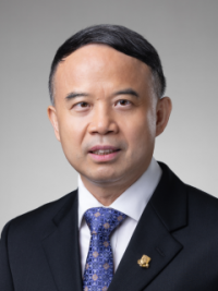](https://www.math.cuhk.edu.hk/sites/default/files/people/zou3_chair.png)
Welcome to the Department of Mathematics at The Chinese University of Hong Kong. Our Department started even before the establishment of the University in 1963. It began as three separate Mathematics Departments in Chung Chi College, New Asia College and United College some 60 years ago, and merged into a single department when the University was formed in 1963.
Over the years, our Department has developed into a world-class Mathematics Department to meet societal needs and global challenges through quality teaching, research and knowledge transfer. We have trained thousands of graduates who have been occupying top positions here in the Hong Kong and the world over. Most noteworthy is our alumnus Prof. S.T. Yau, who obtained the Fields Medal (the highest honor in Mathematics) in 1982.
Mathematics is the foundation of all sciences as it provides the universal language and tools to study and analyze different disciplines. It becomes increasingly important in this day and age when people collect vast amounts of information and data daily via different sources – financial, social, medical, environmental or astronomical. Analyzing these data requires a deep understanding of the mathematical models behind them, and solving the models requires sophisticated mathematical knowledge. The knowledge which a mathematics student would gain from the Department will prepare them for a wide range of careers.
Our Department provides a comprehensive curriculum that covers different aspects of mathematics and various streams of study to cater for the diverse career goals the students may have. We have world-leading researchers in algebra, analysis, geometry, number theory, partial differential equations, scientific computing and topology on our staff list. Even in today’s environment where research always takes the lead, high-quality teaching has always been the hallmark of the Department. As a result, our programme is able to attract top-notch students and has become one of the most competitive programmes within the University.
I invite you to browse our website to learn more about our curriculum and streams of study.
_Jun Zou_
_Choh-Ming Li Chair Professor and Chairman, Department of Mathematics_
---
# Newsletter | CUHK Mathematics
[Skip to main content](#main-content)
[](http://www.cuhk.edu.hk "The Chinese University of Hong Kong")
[](http://www.sci.cuhk.edu.hk/ "Faculty of Science")
[](/ "Home")
Search form
-----------
Search Search Search
[](https://imap.math.cuhk.edu.hk "Math Webmail")
[](/user "Login to this Math Web")
1. [Home](/)
2. [About Us](/about-us)
3. Newsletter
Newsletter
==========
> "Obvious" is the most dangerous word in mathematics.
How obviously do people in mathematics lead a social life? How easily do we believe in popular culture, which portrays people doing mathematics as social misfits? Let our newsletters speak for ourselves.
Real-life mathematicians come from many walks of life. We gather to delve into mathematics, share our insights and celebrate our successes. Past students who have put aside mathematics came to appreciate it even more. From professors' unusual background stories to outgoing students who returned to Hong Kong, many treasures await you here. Achievements, activities, alumni, anecdotes - find out more in our annual newsletter archive.
All submissions are welcome. Please submit your articles using [this form](/about-us/life-cumath/newsletter/submission)
and we will get back to you shortly.
* * *
[](https://www.math.cuhk.edu.hk/sites/default/files/about-us/newsletter/newsletter2223.pdf)
[Issue 20, Year 2022-2023](https://www.math.cuhk.edu.hk/sites/default/files/about-us/newsletter/newsletter2122.pdf)
[](https://www.math.cuhk.edu.hk/sites/default/files/about-us/newsletter/newsletter2122.pdf)
[Issue 19, Year 2021-2022](https://www.math.cuhk.edu.hk/sites/default/files/about-us/newsletter/newsletter2122.pdf)
[](/sites/default/files/about-us/newsletter/newsletter2021.pdf)
[Issue 18, Year 2020-2021](/sites/default/files/about-us/newsletter/newsletter2021.pdf)
[](/sites/default/files/about-us/newsletter/newsletter1920.pdf)
[Issue 17, Year 2019-2020](/sites/default/files/about-us/newsletter/newsletter1920.pdf)
[](/sites/default/files/about-us/newsletter/newsletter1819.pdf)
[Issue 16, Year 2018-201](/sites/default/files/about-us/newsletter/newsletter1819.pdf)
9
[](/sites/default/files/about-us/newsletter/newsletter1718.pdf)
[Issue 15, Year 2017-2018](/sites/default/files/about-us/newsletter/newsletter1718.pdf)
[](/sites/default/files/about-us/newsletter/newsletter1617.pdf)
[Issue 14, Year 2016-2017](/sites/default/files/about-us/newsletter/newsletter1617.pdf)
[](/sites/default/files/about-us/newsletter/newsletter1516.pdf)
[Issue 13, Year 2015-2016](/sites/default/files/about-us/newsletter/newsletter1516.pdf)
[](/sites/default/files/about-us/newsletter/newsletter1415.pdf)
[Issue 12, Year 2014-2015](/sites/default/files/about-us/newsletter/newsletter1415.pdf)
[](/sites/default/files/about-us/newsletter/newsletter1314.pdf)
[Issue 11, Year 2013-2014](/sites/default/files/about-us/newsletter/newsletter1314.pdf)
[](/sites/default/files/about-us/newsletter/newsletter1213.pdf)
[Issue 10, Year 2012-2013](/sites/default/files/about-us/newsletter/newsletter1213.pdf)
[](/sites/default/files/about-us/newsletter/newsletter1112.pdf)
[Issue 9, Year 2011-2012](/sites/default/files/about-us/newsletter/newsletter1112.pdf)
[](/sites/default/files/about-us/newsletter/newsletter1011.pdf)
[Issue 8, Year 2010-2011](/sites/default/files/about-us/newsletter/newsletter1011.pdf)
[](/sites/default/files/about-us/newsletter/newsletter0910.pdf)
[Issue 7, Year 2009-2010](/sites/default/files/about-us/newsletter/newsletter0910.pdf)
[](/sites/default/files/about-us/newsletter/newsletter0809.pdf)
[Issue 6, Year 2008-2009](/sites/default/files/about-us/newsletter/newsletter0809.pdf)
[](/sites/default/files/about-us/newsletter/newsletter0708.pdf)
[Issue 5, Year 2007-2008](/sites/default/files/about-us/newsletter/newsletter0708.pdf)
[](/sites/default/files/about-us/newsletter/newsletter0607.pdf)
[Issue 4, Year 2006-2007](/sites/default/files/about-us/newsletter/newsletter0607.pdf)
[](/sites/default/files/about-us/newsletter/newsletter0506.pdf)
[Issue 3, Year 2005-2006](/sites/default/files/about-us/newsletter/newsletter0506.pdf)
[](/sites/default/files/about-us/newsletter/newsletter0405.pdf)
[Issue 2, Year 2004-2005](/sites/default/files/about-us/newsletter/newsletter0405.pdf)
[](/sites/default/files/about-us/newsletter/newsletter0304.pdf)
[Issue 1, Year 2003-2004](/sites/default/files/about-us/newsletter/newsletter0304.pdf)
* [Issue 15, Year 2017-2018](/sites/default/files/about-us/newsletter/newsletter1718.pdf)
* [Issue 14, Year 2016-2017](/sites/default/files/about-us/newsletter/newsletter1617.pdf)
* [Issue 13, Year 2015-2016](/sites/default/files/about-us/newsletter/newsletter1516.pdf)
* [Issue 12, Year 2014-2015](/sites/default/files/about-us/newsletter/newsletter1415.pdf)
* [Issue 11, Year 2013-2014](/sites/default/files/about-us/newsletter/newsletter1314.pdf)
* [Issue 10, Year 2012-2013](/sites/default/files/about-us/newsletter/newsletter1213.pdf)
* [Issue 9, Year 2011-2012](/sites/default/files/about-us/newsletter/newsletter1112.pdf)
* [Issue 8, Year 2010-2011](/sites/default/files/about-us/newsletter/newsletter1011.pdf)
* [Issue 7, Year 2009-2010](/sites/default/files/about-us/newsletter/newsletter0910.pdf)
* [Issue 6, Year 2008-2009](/sites/default/files/about-us/newsletter/newsletter0809.pdf)
* [Issue 5, Year 2007-2008](/sites/default/files/about-us/newsletter/newsletter0708.pdf)
* [Issue 4, Year 2006-2007](/sites/default/files/about-us/newsletter/newsletter0607.pdf)
* [Issue 3, Year 2005-2006](/sites/default/files/about-us/newsletter/newsletter0506.pdf)
* [Issue 2, Year 2004-2005](/sites/default/files/about-us/newsletter/newsletter0405.pdf)
* [Issue 1, Year 2003-2004](/sites/default/files/about-us/newsletter/newsletter0304.pdf)
---
# Photo Album | CUHK Mathematics
[Skip to main content](#main-content)
[](http://www.cuhk.edu.hk "The Chinese University of Hong Kong")
[](http://www.sci.cuhk.edu.hk/ "Faculty of Science")
[](/ "Home")
Search form
-----------
Search Search Search
[](https://imap.math.cuhk.edu.hk "Math Webmail")
[](/user "Login to this Math Web")
1. [Home](/)
2. [About Us](/about-us)
3. [Life in CU Math](/about-us/life-cumath)
4. Photo Album
Photo Album
===========
### Activities
* * *
#### 2016
[](http://www.math.cuhk.edu.hk/sites/default/files/about-us/life-cumath/photo_day_2016.jpg "Photo Day 2016")
#### 2015
[](/sites/default/files/about-us/life-cumath/img_1662.jpg "Departmental Retreat in 2015")
[](/sites/default/files/about-us/life-cumath/img_7685.jpg "Photo Day 2015")
#### 2013
[](/sites/default/files/about-us/life-cumath/img_3449.jpg "Photo Day 2013")
#### 2012
[](/sites/default/files/about-us/life-cumath/img_6027.jpg "Academic Lecture by Prof. Paul LEE")
###
Souvenirs / Welfare Products
* * *
#### Souvenirs for Orientation Day (for Undergraduate Admissions)
[](/sites/default/files/about-us/life-cumath/file2013.jpg "Souvenirs delivered on O-day 2013")
[](/sites/default/files/about-us/life-cumath/file2014.jpg "Souvenirs delivered on O-day 2014")
---
# Computing Laboratory | CUHK Mathematics
[Skip to main content](#main-content)
[](http://www.cuhk.edu.hk "The Chinese University of Hong Kong")
[](http://www.sci.cuhk.edu.hk/ "Faculty of Science")
[](/ "Home")
Search form
-----------
Search Search Search
[](https://imap.math.cuhk.edu.hk "Math Webmail")
[](/user "Login to this Math Web")
1. [Home](/)
2. [About Us](/about-us)
3. Computing Laboratory
Computing Laboratory
====================
The computing laboratory is mainly used for the teaching of undergraduate courses in Mathematics. Some senior courses in applied and/or computational mathematics are also taught there.
The laboratory has a scanner, black-and-white printers, a whiteboard in the front and a table for quiet discussion at the back. Printer "ug232" is for undergraduates. Undergraduates and postgraduates may print up to 400 and 1500 A4 pages respectively, and each printed side counts as one page.
###
Opening Hours
* * *
The computing laboratory is open 24 hours every day, **with the following exceptions for classes:**
**2022/23 - Term 2**
#### _For MATH2221 A/B/C Mathematics Laboratory II_
#### **Every Tuesday : 10:15 a.m. - 1:30 p.m.**
#### **Every Thursday : 10:15 a.m. - 4:15 p.m.**
#### _For MATH3330 Big Data Computing_
#### **Every Thursday : 4:15 p.m. - 6:30 p.m.**
###
Laboratory Guidelines
* * *
1. **ONLY** Mathematics major students and departmental staff may access the Laboratory. They may only use the computers for valid mathematics courses efficiently and non-wastefully - never for commercial purposes.
2. All users must observe the Laboratory regulations posted at the Laboratory entrance to make the Laboratory safe and comfortable for proper use.
3. All users are automatically governed by the policies in [GEN002 (Computer Network, Policies and Guidelines on Access and Usage)](https://www.itsc.cuhk.edu.hk/it-policies/net-guide-use/)
. The [User Area of ITSC](https://www.itsc.cuhk.edu.hk/all-it/it-facilities/user-areas/)
provides hard copies of these guidelines.
4. We will suspend the Laboratory privileges of any user who violates the guidelines and regulations presented and mentioned here.
5. All users have the responsibility to report:
* system or hardware failure,
* any abuse or wrongful usage of the computer facilities, and
* any attack on the computer security systemto the system administrators in the Laboratory directly.
6. After using a computer, please select LOG OFF / RESTART instead of SHUT DOWN.
###
Notes for the Users
* * *
**Do NOT turn off the air conditioners:**
We frequently find that the air conditioners of our computing lab are turned off. PLEASE DO NOT turn them off under any circumstances. If the air conditioners are found out of order, such as dripping water, please report to the system administrators in the lab or general office staff (in Rm 220) as soon as possible.
_Computer Labs are always low-temperature._
If you feel cool, please put on more clothes before going to the computing lab. Computing equipment is required to work under a certain temperature or their lifespan will be greatly cut short.
---
# Maps & Directions | CUHK Mathematics
[Skip to main content](#main-content)
[](http://www.cuhk.edu.hk "The Chinese University of Hong Kong")
[](http://www.sci.cuhk.edu.hk/ "Faculty of Science")
[](/ "Home")
Search form
-----------
Search Search Search
[](https://imap.math.cuhk.edu.hk "Math Webmail")
[](/user "Login to this Math Web")
1. [Home](/)
2. [About Us](/about-us)
3. Maps & Directions
Maps & Directions
=================
Our teaching buildings are **Lady Shaw Building** for our department, and **Academic Building 1** for the Institute of Mathematical Sciences.
Overnight visitors may free up their time to experience Hong Kong by staying at any of the lodgings closest to us: [Hyatt Regency Hong Kong, Sha Tin](https://www.hyatt.com/en-US/hotel/china/hyatt-regency-hong-kong-sha-tin/shahr)
and [Royal Park Hong Kong Hotel](https://www.royalpark.com.hk/en/)
.
**Tips:**
* Use an Octopus card for bus and MTR journeys.
* This [list of Chinese texts](/sites/default/files/about-us/maps-directions/chinese.pdf)
may help in case the driver does not understand English or Putonghua well.
* The place names "Shatin" and "Sha Tin" are equivalent and may be used interchangeably.
* * *
#### [Hong Kong International Airport : University MTR Station](#hkia_umtr)
Choose one of the following:
* Take the Airport Express which runs every 10 minutes and change at **Tsing Yi**; or
* Take the [circular **S1** bus](http://search.kmb.hk/KMBWebSite/index.aspx?lang=tc)
which runs every 10-15 minutes from the airport to **Tung Chung** MTR Station.
Board the MTR to Lai King. At Lai King, change to Prince Edward in the direction of Yau Ma Tei. Then change to Kowloon Tong in the direction of Lo Wu / Lok Ma Chau, and get off at University. Click [here](http://www.mtr.com.hk/en/customer/jp/index.php?sid=47&eid=71)
for more details.
#### [Hong Kong International Airport : Hyatt Regency Hong Kong, Sha Tin](#hkia_hyatt)
#### By taxi:
A taxi seats at most five. The 40-minute ride costs HKD 350-400 (USD 45-50) subject to traffic conditions. Both red and green taxis are available, the red ones being more expensive. Passengers may request a receipt of payment upon arrival. The address of Hyatt Regency Hong Kong, Shatin is **18 Chak Cheung Street, Shatin**.
* * *
#### By bus:
At the Airport Bus Terminus, take [Airport Bus **A41**](http://search.kmb.hk/KMBWebSite/index.aspx?lang=tc)
. Get off at Shatin Central Bus Terminus of a huge mall known as New Town Plaza in Sha Tin. However it is not the terminal stop for the bus, so ask the driver where to get off, or pay attention to the announcement, and press the red button on the rail when it is the next stop. The frequency is 20 minutes, and the journey takes 45-60 minutes depending on traffic conditions.
Alternatively, [Airport Bus **E42**](http://search.kmb.hk/KMBWebSite/index.aspx?lang=tc)
runs every 20 minutes, and it is a 75-minute trip, while [Airport Bus **N42**](http://search.kmb.hk/KMBWebSite/index.aspx?lang=tc)
is a 1½-hour night bus route and runs at 03:50 am and 04:50 am only.
At Shatin MTR Station, connected by:
* **Taxi**
You can take a taxi to the hotel. The fare is about HK$70. It will take about 15 minutes.
* **MTR Train**
Take the escalator in New Town Plaza, and board the MTR from Sha Tin to University. It is a 9-minute ride. The trains run every 5 to 10 minutes from 06:00 to 24:00. Click [here](http://www.mtr.com.hk/en/customer/jp/index.php?sid=68&eid=71)
for more information. At University MTR Station, take Exit B. You may follow the map below to go to the hotel. The hotel is a three-minute walk from University MTR Station, next to the tall white Cheng Yu Tung building.
#### [Hong Kong International Airport : Royal Park Hong Kong Hotel](#hkia_royal)
#### By taxi:
A taxi seats at most five. The 40-minute ride costs HKD 250 (about USD 30) if traffic is good. You can only take the red-colored taxi (city taxis). Passengers may request a receipt of payment upon arrival. The
address of Royal Park Hotel is **8 Pak Hok Ting Street, Shatin**.
* * *
#### By bus:
At the Airport Bus Terminus, take [Airport Bus **A41**](http://search.kmb.hk/KMBWebSite/index.aspx?lang=tc)
. Get off at the bus stop in front of the Hotel. It should be the second bus stop after a long tunnel. Note that it is not the terminal stop for the bus, so ask the driver where to get off, or pay attention to the announcement and press the red button on the rail when it is the next stop. The frequency is 20 minutes and the journey takes 45-60 minutes depending on traffic conditions. (Please click [here](http://m.kmb.hk/en/result.html?busno=a41#desDetail)
for bus stop information.)
#### [Hyatt Regency Hong Kong, Sha Tin : University MTR Station](#hyatt_umtr)
The hotel is a three-minute walk from University MTR Station, next to the tall white Cheng Yu Tung building.
#### [Royal Park Hong Kong Hotel : University MTR Station](#royal_umtr)
Exit the hotel and turn right. Walk along Hok Ting Street to New Town Plaza. Take the escalator in New Town Plaza, and board the MTR from Sha Tin to University. It is a 9-minute ride. The trains run every 5 to 10 minutes from 06:00 to 24:00.
#### [University MTR Station : Lady Shaw Building](#umtr_lsb)
Take Shuttle Bus **1A** / **1B**/ **2** / **H** near MTR Exit A or Exit C. Get off at the second stop (**Sir Run Run Shaw Hall**).
* [Shuttle Bus Route Information](https://transport.cuhk.edu.hk/route/1a/)
The rooftop garden opposite Sir Run Run Shaw Hall is part of Lady Shaw Building. Go there and enter the lift on the right under the flat canopy. It is a three-minute walk. In particular, the six lecture theatres of Lady Shaw Building (LT1-LT6) are on 1/F.
#### [University MTR Station : Academic Building 1](#umtr_ab1)
#### By car:
Enter the university through the Chung Chi College gate. Pass by the college chapel and drive to the second crossroad. Turn left. Somewhere on the right of the sidewalk is a white building with 7 stories and glass panes. That is Academic Building 1.
* * *
#### By foot:
This is a stroll that takes 10-15 minutes. Get off at Exit C and enter Wu Ho Man Yuen building opposite the road. Exit at 5/F and walk straight, past the student hostels. Cross the driveway and walk along the brick-laid Garden Road, where many sheds and pots are. After a small climb where you reach the top of a hill, turn left and descend the wavy brick road. At the crossroad (a driveway), turn right and keep to the sidewalk.
Somewhere on the right of the sidewalk is a white building with 7 stories and glass panes. That is Academic Building 1.
#### [Lady Shaw Building : Academic Building 1](#lsb_ab1)
Leave Lady Shaw Building via Exit D to LG1/F. Walk along the footbridge to the clearing. Choose one of the following:
* Turn left, walk along the bridge (2/3 covered, 1/3 open-air) and enter Mong Man Wai Engineering Building. Turn right and take the express lift from 9/F to 4/F. Exit the glass doors on your left. Walk straight through the car park until you reach the foot of a flight of stairs.
* Turn right and enter the glass door to Ho Sin Hang Engineering Building. (Do not enter the one that has the view of the Tolo Harbour.) Take the lift from 5/F to G/F. Exit the lift on your right and turn right. Then exit the glass doors leading to a staircase, not the car park. Walk down the staircase.
Walk down the road. Somewhere on the left of the sidewalk is a white building with 7 stories and glass panes. That is Academic Building 1.
To travel from Academic Building 1 to Lady Shaw Building, reverse the steps above.
---
# Contact Us | CUHK Mathematics
[Skip to main content](#main-content)
[](http://www.cuhk.edu.hk "The Chinese University of Hong Kong")
[](http://www.sci.cuhk.edu.hk/ "Faculty of Science")
[](/ "Home")
Search form
-----------
Search Search Search
[](https://imap.math.cuhk.edu.hk "Math Webmail")
[](/user "Login to this Math Web")
1. [Home](/)
2. [About Us](/about-us)
3. Contact Us
Contact Us
==========
**Address**
Department of Mathematics,
Room 220, Lady Shaw Building,
The Chinese University of Hong Kong,
Shatin, N.T., Hong Kong
**Tel**
(852) 3943-7988
**Fax**
(852) 2603-5154
**Email**
[dept@math.cuhk.edu.hk](mailto:dept@math.cuhk.edu.hk)
**URL**
[http://www.math.cuhk.edu.hk/](http://www.math.cuhk.edu.hk/)
###
Opening Hours
* * *
#### General Office
**Monday to Thursday:**
8:45 am to 1:00 pm, 2:00 pm to 5:30 pm
**Friday:**
8:45 am to 1:00 pm, 2:00 pm to 5:45 pm
**Remarks:**
* Telephone recording is available for students/public enquiries. Enquiries or service requests may be made by post, fax or electronic means.
* Saturday classes of postgraduate/self-financed programmes remain unchanged.
* * *
#### Computing Laboratory
**Monday to Sunday:**
24 hours
**Remarks:**
Please refer to the page of [Computing Laboratory](/about-us/computing-laboratory)
for lab classes schedules
---
# Career Opportunities | CUHK Mathematics
[Skip to main content](#main-content)
[](http://www.cuhk.edu.hk "The Chinese University of Hong Kong")
[](http://www.sci.cuhk.edu.hk/ "Faculty of Science")
[](/ "Home")
Search form
-----------
Search Search Search
[](https://imap.math.cuhk.edu.hk "Math Webmail")
[](/user "Login to this Math Web")
1. [Home](/)
2. [About Us](/about-us)
3. Career Opportunities
Career Opportunities
====================
We currently have the following opening(s):
### **Professor / Associate Professor / Assistant Professor**
Founded in 1963, The Chinese University of Hong Kong (CUHK) is a forward-looking comprehensive research university with a global vision and a mission to combine tradition with modernity, and to bring together China and the West. The Department of Mathematics in CUHK has developed a strong reputation in teaching and research. Many of the faculty members are internationally renowned and are recipients of prestigious awards and honours. The graduates are successful in both academia and industry. The Department is highly ranked internationally, e.g., it is 41st, 66th and 63rd in the 2022, 2023 and 2024 QS World University Rankings, and 51st, 42nd and 56th in the 2022, 2023 and 2024 US News Rankings, respectively.
The Department is now inviting applications for substantiable-track faculty posts at all the academic levels, one for algebra and related areas, one for general areas of mathematics (with priority on harmonic analysis/geometric analysis), and two in applied and computational mathematics, beginning in August 2025. Applicants should have (i) a relevant PhD degree in mathematics or related disciplines; (ii) an established track record in research, including publications; and (iii) a demonstrated commitment to excellence in teaching.
Applicants should arrange at least 3 reference letters, 2 on research and 1 on teaching, to be submitted by the reference writers.
Appointment will normally be made on contract basis for up to three years initially commencing August 2025, which, subject to mutual agreement, may lead to substantiation or longer-term appointment later. Review of applications will begin on 1 December, 2024, and will continue until the positions are filled.
Submission an application: [https://www.mathjobs.org/jobs/list/25175](https://www.mathjobs.org/jobs/list/25175)
### **Research Assistant Professor / Postdoctoral Fellows**
Founded in 1963, The Chinese University of Hong Kong (CUHK) is a forward-looking comprehensive research university with a global vision and a mission to combine tradition with modernity, and to bring together China and the West. The Department of Mathematics in CUHK has developed a strong reputation in teaching and research. Many of the faculty members are internationally renowned and are recipients of prestigious awards and honours. The graduates are successful in both academia and industry. The Department is highly ranked internationally, e.g., it is 41st, 66th and 63rd in the 2022, 2023 and 2024 QS World University Rankings, and 51st, 42nd and 56th in the 2022, 2023 and 2024 US News Rankings, respectively.
The Department has multiple openings for Research Assistant Professors and Postdoctoral Fellows. The Department is now cordially inviting applications for non-substantiable posts at Research Assistant Professor (RAP) / Postdoctoral Fellow (Post-doc) levels in all areas of Mathematics beginning in August 2025. We seek promising young mathematicians whose research areas match the areas of our faculty members. The RAP and Post-doc positions are for three-year and two-year durations, respectively, with possible extension. The teaching load of these appointments is light, with one course each academic year. Applicants should have (i) a PhD degree in mathematics or related disciplines; and (ii) demonstrated potential for research and teaching.
Applicants should arrange at least 3 reference letters, 2 on research and 1 on teaching, to be submitted by the reference writers.
Review of applications will begin on 1 December, 2024 and will continue until the positions are filled.
Submit an application: [https://www.mathjobs.org/jobs/list/25141](https://www.mathjobs.org/jobs/list/25141)
The University reserves the right to appoint by invitation.
* * *
* * *
---
# User account | CUHK Mathematics
[Skip to main content](#main-content)
[](http://www.cuhk.edu.hk "The Chinese University of Hong Kong")
[](http://www.sci.cuhk.edu.hk/ "Faculty of Science")
[](/ "Home")
Search form
-----------
Search Search Search
[](https://imap.math.cuhk.edu.hk "Math Webmail")
[](/user "Login to this Math Web")
1. [Home](/)
2. [User account](/user)
3. Request new password
User account
============
Primary tabs
------------
* [Log in](/user)
* [Request new password(active tab)](/user/password)
Username or e-mail address \*
E-mail new password
---
# Honours & Awards by Current and Former Faculty Members | CUHK Mathematics
[Skip to main content](#main-content)
[](http://www.cuhk.edu.hk "The Chinese University of Hong Kong")
[](http://www.sci.cuhk.edu.hk/ "Faculty of Science")
[](/ "Home")
Search form
-----------
Search Search Search
[](https://imap.math.cuhk.edu.hk "Math Webmail")
[](/user "Login to this Math Web")
1. [Home](/)
2. [Research](/research)
3. [Honours & Awards](/research/honours-awards)
4. Honours & Awards by Current and Former Faculty Members
Honours & Awards by Current and Former Faculty Members
======================================================
* * *
#### [2021 - present](#collapse2021)
#### **2024**
* * *
* **Recipient for HKSAR Global STEM Professorship Scheme**
* ****Prof. Juncheng WEI
* **National Science Fund for Distinguished Young Scholars (國家傑出青年科學基金項目)**
* ****Prof. Renjun DUAN
* **Asian Young Scientist Fellowship 2024**
* Prof. Man Chun LEE
#### **2023**
* * *
* **Faculty Exemplary Teaching Award**
* Prof. Ronald Lok Ming LUI
#### **2022**
* * *
* **Recipient for HKSAR Global STEM Professorship Scheme**
* ****Prof. Bangti JIN
* **New Cornerstone Investigator (新基石研究員), Tencent Foundation**
* Prof. Xuhua HE
* **ICCM Silver Medal of Mathematics**
* Prof. Eric Tsz Shun CHUNG
* **Fellow, American Mathematical Society (AMS)**
* Prof. Jun ZOU ([link](http://www.ams.org/cgi-bin/fellows/fellows_by_year.cgi)
)
* **Chevalley Prize, American Mathematical Society (AMS)**
* Prof. Xuhua HE ([link](https://www.ams.org/news?news_id=6828)
)
* **Outstanding Fellow, Faculty of Science (CUHK)**
* Prof. Eric Tsz Shun CHUNG
* **Faculty Exemplary Teaching Award**
* Dr. Man Chuen CHENG
#### **2021**
* * *
* **Antonio Ambrosetti Medal**
* Prof. Po Lam YUNG ([link](https://www.math.sissa.it/content/antonio-ambrosetti-medal)
)
* **Early Career Award, Research Grant Council**
* Prof. Liu LIU
* Prof. Chenyun LUO
* Prof. Michael McBREEN
* **Hong Kong Mathematical Society Young Scholar Award**
* Prof. Martin Man Chun LI
* Prof. Tieyong ZENG
* **Faculty Exemplary Teaching Award**
* Dr. Kai Leung CHAN
#### [2016 - 2020](#collapse2016)
#### **2020**
* * *
* **XPLORER Prize 2020 (科學探索獎 2020), XPLORER Prize Foundation**
* Prof. Xuhua HE
* **Excellent Young Scientists Fund 2020, National Natural Science Foundation of China (NSFC)**
* ****Prof. Martin Man Chun LI
* **Hong Kong Mathematical Society Young Scholar Award**
* Prof. Kwok Wai CHAN
* Prof. Renjun DUAN
* **Faculty Exemplary Teaching Award**
* Prof. Martin Man Chun LI
#### **2019**
* * *
* **Fellow, Society for Industrial and Applied Mathematics**
* Prof. Jun ZOU
* **Member, Academy of Science, The Royal Society of Canada**
* Prof. Juncheng WEI
* **Zhong Jia Qin Mathematics Award**
* Prof. Guohuan QIU
* **Qin Yuanxun Mathematical Award, Qin Yuanxun Mathematical Prize Foundation**
* Prof. Zhouping XIN
* **ICCM Best paper award**
* Prof. Kwok Wai CHAN
* Prof. Conan Nai Chung LEUNG
* **University Exemplary Teaching Award in General Education**
* Dr. Chi Hin LAU
* **Vice-Chancellor's Exemplary Teaching Award**
* Prof. Ronald Lok Ming LUI
* **Faculty Exemplary Teaching Award**
* Prof. Ronald Lok Ming LUI
#### **2018**
* * *
* **Hong Kong Mathematical Society Young Scholar Award**
* Prof. Ronald Lok Ming LUI
* **Distinguished Paper Award, International Consortium of Chinese Mathematicians Best Paper Award**
* Prof. Luen Fai TAM
* Prof. Zhongtao WU
* Prof. Po Lam YUNG
* **Faculty Exemplary Teaching Award**
* Dr. Mark Jingjing XIAO
* **ICCM Best Paper Award**
* Prof. Xuhua HE
* Prof. Zhouping XIN
* **ICM Invited Speaker**
* Prof. Xuhua HE
#### **2017**
* * *
* **Vice-Chancellor's Exemplary Teaching Award**
* Prof. Kwok Wai CHAN
* **Distinguished Paper Award and Silver Award, International Consortium of Chinese Mathematicians Best Paper Award**
* Prof. Kwok Wai CHAN
* Prof. Conan N. C. LEUNG
* **Hong Kong Mathematical Society Young Scholar Award**
* Prof. Eric Tsz Shun CHUNG
* **Faculty Exemplary Teaching Award**
* Prof. Kwok Wai CHAN
* **Distinguished Paper Award, International Consortium of Chinese Mathematicians**
* Prof. Ronald Lok Ming LUI
#### **2016**
* * *
* **Paul Erdős Award**
* Prof. Kar-Ping SHUM
* **Faculty Exemplary Teaching Award**
* Prof. Po Lam YUNG
* **International Conference on Representations of Algebras Award (ICRA Award)**
* Prof. Yu QIU
* **Morningside Silver Medal of Mathematics**
* Prof. Ronald Lok Ming LUI
#### [2011 - 2015](#collapse2011)
#### **2015**
* * *
* **Faculty Exemplary Teaching Award**
* Dr. Wing Chung FONG
* **Early Career Award, Research Grant Council**
* Prof. Po Lam YUNG
* **University Education Award 2014/15**
* Prof. Thomas Kwok Keung AU
* **Invited Speaker of Current development of Mathematics conference**
* Prof. Xuhua HE
#### **2014**
* * *
* **The China National Thousands Talents Program**
* Prof. Jun ZOU
* **Faculty Exemplary Teaching Award**
* ****Prof. Ronald Lok Ming LUI
* **Fellow, American Mathematical Society (AMS)**
* Prof. Zhouping XIN
#### **2013**
* * *
* **Fellow, American Mathematical Society (AMS)**
* Prof. Conan Nai Chung LEUNG
* Prof. Jiu-Kang YU
* **Fellow, Society for Industrial and Applied Mathematics**
* Prof. Raymond Honfu CHAN
* **Faculty Exemplary Teaching Award**
* Prof. Chi Wai LEUNG
* **Morningside Gold Medal of Mathematics**
* Prof. Xuhua HE
* **Croucher Fellowship for Postdoctoral Research**
* Prof. Martin Man Chun LI
#### **2012**
* * *
* **Faculty Exemplary Teaching Award**
* Prof. Kai Seng CHOU
#### **2011**
* * *
* **Faculty Exemplary Teaching Award**
* Prof. Thomas Kwok Keung AU
* **Natural Science Award First-class Award**
* Prof. Raymond Honfu CHAN
* **Vice-Chancellor's Exemplary Teaching Award**
* Prof. Thomas Kwok Keung AU
#### [2006 - 2010](#collapse2006)
#### **2010**
* * *
* **ICCM Chern Prize**
* Prof. Conan Nai Chung LEUNG
* **Faculty Exemplary Teaching Award**
* Dr. Jeff Chak Fu WONG
* **Natural Science Award First-class Award**
* Prof. Juncheng WEI
* **Research Excellence Award, CUHK**
* Prof. Juncheng WEI
#### **2009**
* * *
* **Faculty Exemplary Teaching Award**
* Prof. Dejun FENG
#### **2008**
* * *
* **Faculty Exemplary Teaching Award**
* Dr. Leung Fu CHEUNG
#### **2007**
* * *
* **Faculty Exemplary Teaching Award**
* Prof. Thomas Kwok Keung AU
* **Morningside Gold Medal**
* Prof. Zhouping XIN
#### **2006**
* * *
* **Faculty Exemplary Teaching Award**
* Prof. Chi Wai LEUNG
#### [2001 - 2005](#collapse2001)
#### **2005**
* * *
* **Faculty Exemplary Teaching Award**
* Dr. Ka Lun CHEUNG
* **Croucher Senior Research Fellowship**
* Prof. Juncheng WEI
#### **2004**
* * *
* **Faculty Exemplary Teaching Award**
* Prof. Thomas Kwok Keung AU
* **The Young Researcher Award, CUHK**
* Prof. Juncheng WEI
#### **2003**
* * *
* **Faculty Exemplary Teaching Award**
* Prof. Luen Fai TAM
#### **2002**
* * *
* **Faculty Exemplary Teaching Award**
* Prof. Kung Fu NG
* **ICM invited speaker**
* Prof. Zhouping XIN
* **Vice-Chancellor's Exemplary Teaching Award**
* Prof. Kung Fu NG
#### **2001**
* * *
* **Faculty Exemplary Teaching Award**
* ****Prof. Hing Sun LUK
* **ICCM Chern Prize**
* Prof. Jiu Kang YU
#### [1996 - 2000](#collapse1996)
#### **2000**
* * *
* **Faculty Exemplary Teaching Award**
* ****Prof. Luen Fai TAM
#### **1999**
* * *
* **Faculty Exemplary Teaching Award**
* ****Prof. Kung Fu NG
---
# Professors | CUHK Mathematics
[Skip to main content](#main-content)
[](http://www.cuhk.edu.hk "The Chinese University of Hong Kong")
[](http://www.sci.cuhk.edu.hk/ "Faculty of Science")
[](/ "Home")
Search form
-----------
Search Search Search
[](https://imap.math.cuhk.edu.hk "Math Webmail")
[](/user "Login to this Math Web")
1. [Home](/)
2. [People](/people)
3. [Academic Staff](/people/academic-staff)
4. Professors
Professors
==========
| | | | |
| --- | --- | --- | --- |
### Professor of Mathematics
| **[Prof. Bangti JIN (Global STEM Scholar)](/people/academic-staff/btjin)
** | LSB 215 | 3943 6777 | [b.jin@cuhk.edu.hk](mailto:b.jin@cuhk.edu.hk) |
| **[Prof. Conan Nai Chung LEUNG](/people/academic-staff/leung)
** | AB1 506 | 3943 8065 | [leung@math.cuhk.edu.hk](mailto:leung@math.cuhk.edu.hk) |
| **[Prof. Juncheng Wei
(Global STEM Scholar)](https://www.math.cuhk.edu.hk/people/academic-staff/wei)
** | LSB 201 | 3943 7970 | [wei@math.cuhk.edu.hk](mailto:wei@math.cuhk.edu.hk) |
| **[Prof. Zhouping XIN](/people/academic-staff/zpxin)
** | AB1 701 | 3943 4100 | [zpxin@ims.cuhk.edu.hk](mailto:zpxin@ims.cuhk.edu.hk) |
| **[Prof. Shing Tung YAU](/people/academic-staff/yau)
** | LSB 102 | 3943 7968 | [yau@ims.cuhk.edu.hk](mailto:yau@ims.cuhk.edu.hk) |
| **[Prof. Jiu Kang YU](/people/academic-staff/jkyu)
** | AB1 411 | 3943 3716 | [jkyu@ims.cuhk.edu.hk](mailto:jkyu@ims.cuhk.edu.hk) |
| **[Prof. Jun ZOU](/people/academic-staff/zou)
** | LSB 224 | 3943 7967 | [zou@math.cuhk.edu.hk](mailto:zou@math.cuhk.edu.hk) |
| | | | |
| --- | --- | --- | --- |
### Professor
| **[Prof. Kwok Wai CHAN](/people/academic-staff/kwchan)
** | LSB 212 | 3943 7976 | [kwchan@math.cuhk.edu.hk](mailto:kwchan@math.cuhk.edu.hk) |
| **[Prof. Eric Tsz Shun CHUNG](/people/academic-staff/tschung)
** | LSB 205 | 3943 7972 | [tschung@math.cuhk.edu.hk](mailto:tschung@math.cuhk.edu.hk) |
| **[Prof. Renjun DUAN](/people/academic-staff/rjduan)
** | LSB 206 | 3943 7977 | [rjduan@math.cuhk.edu.hk](mailto:rjduan@math.cuhk.edu.hk) |
| **[Prof. Dejun FENG](/people/academic-staff/djfeng)
** | LSB 211 | 3943 7965 | [djfeng@math.cuhk.edu.hk](mailto:djfeng@math.cuhk.edu.hk) |
| **[Prof. Yi Jen LEE](/people/academic-staff/yjlee)
** | AB1 412 | 3943 3715 | [yjlee@math.cuhk.edu.hk](mailto:yjlee@math.cuhk.edu.hk) |
| **[Prof. Ronald Lok Ming LUI](/people/academic-staff/lmlui)
** | LSB 207 | 3943 7975 | [lmlui@math.cuhk.edu.hk](mailto:lmlui@math.cuhk.edu.hk) |
| **[Prof. Xiaolu TAN](/people/academic-staff/xltan)
** | LSB 227 | 3943 5296 | [xltan@math.cuhk.edu.hk](mailto:xltan@math.cuhk.edu.hk) |
| **[Prof. Tieyong ZENG](/people/academic-staff/zeng)
** | LSB 225 | 3943 7966 | [zeng@math.cuhk.edu.hk](mailto:zeng@math.cuhk.edu.hk) |
| | | | |
| --- | --- | --- | --- |
### Associate Professor
| [**Prof. Martin Man Chun LI**](https://www.math.cuhk.edu.hk/people/academic-staff/martinli) | LSB 236 | 3943 1851 | [martinli@math.cuhk.edu.hk](mailto:martinli@math.cuhk.edu.hk) |
| **[Prof. Zhongtao WU](/people/academic-staff/ztwu)
** | LSB 216 | 3943 8578 | [ztwu@math.cuhk.edu.hk](mailto:ztwu@math.cuhk.edu.hk) |
| **[Prof. Yong YU](/people/academic-staff/yongyu)
** | LSB 214 | 3943 8900 | [yongyu@math.cuhk.edu.hk](mailto:yongyu@math.cuhk.edu.hk) |
| | | | |
| --- | --- | --- | --- |
### Assistant Professor
| [**Prof. Gary Pui Tung CHOI
(Vice-Chancellor Assistant Professor)**](https://www.math.cuhk.edu.hk/people/academic-staff/ptchoi) | LSB 204 | 3943 5481 | [ptchoi@math.cuhk.edu.hk](mailto:ptchoi@math.cuhk.edu.hk) |
| **[Prof. Omar KIDWAI](https://www.math.cuhk.edu.hk/people/academic-staff/kidwai)
** | LSB 226 | 3943 7954 | [kidwai@math.cuhk.edu.hk](mailto:kidwai@math.cuhk.edu.hk) |
| **[Prof. Man Chun LEE](https://www.math.cuhk.edu.hk/people/academic-staff/mclee)
** | LSB 237 | 3943 5137 | [mclee@math.cuhk.edu.hk](mailto:mclee@math.cuhk.edu.hk) |
| **[Prof. Liu LIU](/people/academic-staff/lliu)
** | LSB 234 | 3943 7957 | [lliu@math.cuhk.edu.hk](mailto:lliu@math.cuhk.edu.hk) |
| [**Prof. Chenyun LUO**](/people/academic-staff/cluo) | LSB 213 | 3943 7981 | [cluo@math.cuhk.edu.hk](mailto:cluo@math.cuhk.edu.hk) |
| [**Prof. Michael McBREEN**](/people/academic-staff/mcb) | LSB 235 | 3943 5297 | [mcb@math.cuhk.edu.hk](mailto:mcb@math.cuhk.edu.hk) |
| **[Prof. Ziquan YANG
(Chiu Chin Yin Assistant Professor of Mathematics)](https://www.math.cuhk.edu.hk/people/academic-staff/zqyang)
** | AB1 410 | 3943 3717 | [zqyang@math.cuhk.edu.hk](mailto:zqyang@math.cuhk.edu.hk) |
| | | | |
| --- | --- | --- | --- |
### Research Assistant Professor
| [**Prof. Fenglei FAN**](/people/academic-staff/flfan) | LSB232A | 3943 7978 | [flfan@math.cuhk.edu.hk](mailto:flfan@math.cuhk.edu.hk) |
| [**Prof. Kuang HUANG**](https://www.math.cuhk.edu.hk/people/academic-staff/khuang) | LSB237A | 3943 5139 | [khuang@math.cuhk.edu.hk](mailto:khuang@math.cuhk.edu.hk) |
| [**Prof. Jin TAN**](https://www.math.cuhk.edu.hk/people/academic-staff/jtan) | LSB237A | 3943 5139 | [jtan@math.cuhk.edu.hk](mailto:jtan@math.cuhk.edu.hk) |
---
# Administrative Staff | CUHK Mathematics
[Skip to main content](#main-content)
[](http://www.cuhk.edu.hk "The Chinese University of Hong Kong")
[](http://www.sci.cuhk.edu.hk/ "Faculty of Science")
[](/ "Home")
Search form
-----------
Search Search Search
[](https://imap.math.cuhk.edu.hk "Math Webmail")
[](/user "Login to this Math Web")
1. [Home](/)
2. [People](/people)
3. Administrative Staff
Administrative Staff
====================
| | | | |
| --- | --- | --- | --- |
### Administrative Support
| **Ms. Elaine CHAN**
Executive Officer | LSB 221 | 3943 7946 | [elaine.chan@cuhk.edu.hk](mailto:elaine.chan@cuhk.edu.hk) |
| **Ms. Sardonna CHEUNG**
Project Coordinator | LSB 220 | 3943 5295 | [sardonna.cheung@cuhk.edu.hk](mailto:sardonna.cheung@cuhk.edu.hk) |
| **Ms. Joanne HO**
Project Coordinator | LSB 220 | 3943 5482 | [joanne@math.cuhk.edu.hk](mailto:joanne@math.cuhk.edu.hk) |
| **Ms. Amber LAM**
Project Coordinator | LSB 220 | 3943 8608 | [AmberLam@cuhk.edu.hk](mailto:AmberLam@cuhk.edu.hk) |
| **Ms. Janice WONG**
Project Coordinator | LSB 220 | 3943 7729 | [janicewyk@cuhk.edu.hk](mailto:janicewyk@cuhk.edu.hk) |
| **Miss Pauline CHAN**
Clerk | LSB 220 | 3943 7988 | [pauline@math.cuhk.edu.hk](mailto:pauline@math.cuhk.edu.hk) |
| **Miss Suki CHAN**
Clerk | LSB 220 | 3943 7989 | [suki@math.cuhk.edu.hk](mailto:suki@math.cuhk.edu.hk) |
| **Ms. Jenny LAM**
Office Assistant | LSB 220 | 3943 5295 | [jenny@math.cuhk.edu.hk](mailto:jenny@math.cuhk.edu.hk) |
| | | | |
| --- | --- | --- | --- |
### Technical Support
| **Mr. Michael AU YEUNG**
Assistant Computer Officer | LSB 232B | 3943 1897 | [michael@math.cuhk.edu.hk](mailto:michael@math.cuhk.edu.hk) |
| **Mr. Feilan LIU**
Assistant Computer Officer | LSB 232B | 3943 7735 | [flliu@math.cuhk.edu.hk](mailto:flliu@math.cuhk.edu.hk) |
| | | | |
| --- | --- | --- | --- |
### Research / Teaching Support
| **Dr. Xiaoli LIN**
Teaching Assistant | LSB 232A | 3943 7978 | [xllin@math.cuhk.edu.hk](mailto:xllin@math.cuhk.edu.hk) |
| **Dr. Shang Yi LIU**
Teaching Assistant | LSB 232A | 3943 7978 | [syliu@math.cuhk.edu.hk](mailto:syliu@math.cuhk.edu.hk) |
| **Dr. Hiu Ying MAN**
Teaching Assistant | LSB 223 | 3943 7971 | [mhyman@math.cuhk.edu.hk](mailto:mhyman@math.cuhk.edu.hk) |
---
# Administration | CUHK Mathematics
[Skip to main content](#main-content)
[](http://www.cuhk.edu.hk "The Chinese University of Hong Kong")
[](http://www.sci.cuhk.edu.hk/ "Faculty of Science")
[](/ "Home")
Search form
-----------
Search Search Search
[](https://imap.math.cuhk.edu.hk "Math Webmail")
[](/user "Login to this Math Web")
1. [Home](/)
2. [People](/people)
3. Administration
Administration
==============
| | | | |
| --- | --- | --- | --- |
### Department Chair
| [**Prof. Jun ZOU**](https://www.math.cuhk.edu.hk/people/academic-staff/zou) | LSB 224 | 3943 7967 | [zou@math.cuhk.edu.hk](mailto:zou@math.cuhk.edu.hk) |
| | | | |
| --- | --- | --- | --- |
### Deputy Chair
| **[Prof. Ronald Lok Ming LUI](https://www.math.cuhk.edu.hk/people/academic-staff/lmlui)
(Research)** | LSB 207 | 3943 7975 | [lmlui@math.cuhk.edu.hk](mailto:lmlui@math.cuhk.edu.hk) |
| **[Prof. Kwok Wai CHAN](https://www.math.cuhk.edu.hk/people/academic-staff/kwchan)
(Administration)** | LSB 212 | 3943 7976 | [kwchan@math.cuhk.edu.hk](mailto:kwchan@math.cuhk.edu.hk) |
| | | | |
| --- | --- | --- | --- |
### Head of Graduate Admission
| [**Prof. Dejun FENG**](https://www.math.cuhk.edu.hk/people/academic-staff/djfeng) | LSB 211 | 3943 7965 | [djfeng@math.cuhk.edu.hk](mailto:djfeng@math.cuhk.edu.hk) |
| | | | |
| --- | --- | --- | --- |
### Director of MSc Programme
| **[Prof. Renjun DUAN](https://www.math.cuhk.edu.hk/people/academic-staff/rjduan)
** | LSB 206 | 3943 7977 | [rjduan@math.cuhk.edu.hk](mailto:rjduan@math.cuhk.edu.hk) |
| | | | |
| --- | --- | --- | --- |
### Associate Director of MSc Programme
| **[Prof. Chi Wai LEUNG](https://www.math.cuhk.edu.hk/people/academic-staff/cwleung)
** | LSB 204 | 3943 7982 | [cwleung@math.cuhk.edu.hk](mailto:cwleung@math.cuhk.edu.hk) |
| **[Dr. Man Chuen CHENG](https://www.math.cuhk.edu.hk/people/academic-staff/mccheng)
** | LSB 210 | 3943 7985 | [mccheng@math.cuhk.edu.hk](mailto:mccheng@math.cuhk.edu.hk) |
| | | | |
| --- | --- | --- | --- |
### Admission
| **[Prof. Kwok Wai CHAN](/people/academic-staff/kwchan)
** | LSB 212 | 3943 7976 | [kwchan@math.cuhk.edu.hk](mailto:kwchan@math.cuhk.edu.hk) |
| | | | |
| --- | --- | --- | --- |
### Academic Counselling
| [**Prof. Martin Man Chun LI**](https://www.math.cuhk.edu.hk/people/academic-staff/martinli) | LSB 236 | 3943 1851 | [martinli@math.cuhk.edu.hk](mailto:martinli@math.cuhk.edu.hk) |
| | | | |
| --- | --- | --- | --- |
### COSINE Program
| **[Prof. Eric Tsz Shun CHUNG](/people/academic-staff/tschung)
** | LSB 205 | 3943 7972 | [tschung@math.cuhk.edu.hk](mailto:tschung@math.cuhk.edu.hk) |
| | | | |
| --- | --- | --- | --- |
### Scholarship
| **[Prof. Renjun DUAN](https://www.math.cuhk.edu.hk/people/academic-staff/rjduan)
** | LSB 206 | 3943 7977 | [rjduan@math.cuhk.edu.hk](mailto:rjduan@math.cuhk.edu.hk) |
| | | | |
| --- | --- | --- | --- |
### College Coordinators
| #### Chung Chi College | | | |
| [**Dr. Hiu Ning CHAN**](https://www.math.cuhk.edu.hk/people/academic-staff/hnchan) | LSB 233 | 3943 7956 | [hnchan@math.cuhk.edu.hk](mailto:hnchan@math.cuhk.edu.hk) |
| #### New Asia College | | | |
| [**Prof. Michael McBREEN**](https://www.math.cuhk.edu.hk/people/academic-staff/mcb) | LSB 235 | 3943 5297 | [mcb@math.cuhk.edu.hk](mailto:mcb@math.cuhk.edu.hk) |
| #### United College | | | |
| **[Prof. Zhongtao WU](https://www.math.cuhk.edu.hk/people/academic-staff/ztwu)
** | LSB 216 | 3943 8578 | [ztwu@math.cuhk.edu.hk](mailto:ztwu@math.cuhk.edu.hk) |
| #### Shaw College | | | |
| **[Prof. Xiaolu TAN](https://www.math.cuhk.edu.hk/people/academic-staff/xltan)
** | LSB 227 | 3943 5296 | [xltan@math.cuhk.edu.hk](mailto:xltan@math.cuhk.edu.hk) |
---
# People | CUHK Mathematics
[Skip to main content](#main-content)
[](http://www.cuhk.edu.hk "The Chinese University of Hong Kong")
[](http://www.sci.cuhk.edu.hk/ "Faculty of Science")
[](/ "Home")
Search form
-----------
Search Search Search
[](https://imap.math.cuhk.edu.hk "Math Webmail")
[](/user "Login to this Math Web")
1. [Home](/)
2. People
People
======
From the mathematics departments of three colleges to a centre marked by exemplary teaching and research, our first-rate mathematicians are united in their passion for the subject and their love for CUHK and Hong Kong. Our research postgraduates and teaching/research assistants also contribute to our growing body of mathematical work.
Our dedicated support staff teams help us run the Department every day. They are based in the main office or the computing laboratory, both on 2/F of Lady Shaw Building.
---
# Academic Staff | CUHK Mathematics
[Skip to main content](#main-content)
[](http://www.cuhk.edu.hk "The Chinese University of Hong Kong")
[](http://www.sci.cuhk.edu.hk/ "Faculty of Science")
[](/ "Home")
Search form
-----------
Search Search Search
[](https://imap.math.cuhk.edu.hk "Math Webmail")
[](/user "Login to this Math Web")
1. [Home](/)
2. [People](/people)
3. Academic Staff
Academic Staff
==============
[Professors](/people/academic-staff/professors)
------------------------------------------------
[Emeritus / Adjunct Professors](/people/academic-staff/emeritus-adjunct-professors)
------------------------------------------------------------------------------------
[Lecturers](/people/academic-staff/lecturers)
----------------------------------------------
[Post-Doctoral Fellows](/people/academic-staff/post-doctoral-fellows)
----------------------------------------------------------------------
---
# Alumni | CUHK Mathematics
[Skip to main content](#main-content)
[](http://www.cuhk.edu.hk "The Chinese University of Hong Kong")
[](http://www.sci.cuhk.edu.hk/ "Faculty of Science")
[](/ "Home")
Search form
-----------
Search Search Search
[](https://imap.math.cuhk.edu.hk "Math Webmail")
[](/user "Login to this Math Web")
1. [Home](/)
2. [People](/people)
3. Alumni
Alumni
======
We are honoured to have outstanding graduates in education, academia and industry. They are making a difference in our lives, be they in the limelight or behind the scenes.
* Launched in 2016, our [Alumni Association](/alumni-association)
connects our alumni, and supports the development of the Department.
* [Distinguished Alumni](/people/alumni/distinguished-alumni)
recognizes distinguished past students who have risen to prominence in their fields of interest.
* [Further Graduate Studies](/people/further-graduate-studies)
keeps a record of our students who pursue further graduate studies, preparing themselves for careers in both academia and industry.
* [PhD Careers](/people/phd-careers)
lists the first jobs of our PhD graduates.
---
# Constitution | CUHK Mathematics
[Skip to main content](#main-content)
[](http://www.cuhk.edu.hk "The Chinese University of Hong Kong")
[](http://www.sci.cuhk.edu.hk/ "Faculty of Science")
[](/ "Home")
Search form
-----------
Search Search Search
[](https://imap.math.cuhk.edu.hk "Math Webmail")
[](/user "Login to this Math Web")
1. [Home](/)
2. [People](/people)
3. [Alumni](/people/alumni)
4. [Alumni Association](/people/alumni/alumni-association)
5. Constitution
Constitution
============
### 香港中文大學數學系校友會會章
####
第一章 總則
第一條 本會定名為香港中文大學數學系校友會
(英文名稱CUHK Mathematics Alumni Association),以下簡稱本會。
第二條 本會以香港中文大學數學系校友為基礎,以社團形式組成。
第三條 本會宗旨是:加強會員之關係及團結,促進會員福利及協助數學系之發展。
第四條 本會活動包括:
(一) 加強會員間之聯誼、聯繫、資訊交流以及維護會員間之共同利益。
(二) 加強會員與數學系及在學同學之間的聯繫。
(三) 舉辦文娛、學術、體育及聯誼活動等。
(四) 參加及支持香港中文大學各種活動。
(五) 建立和鞏固數學系與社會之間的良好關係。
第五條 本會會址設於香港新界沙田香港中文大學數學系。
第六條 本會以中文為法定語文,以中文及英文為工作語文。
####
第二章 會員
第一條 會員資格:
(1) 基本會員資格:
(a) 1963年香港中文大學成立以後曾在數學系畢業或肄業者;或
(b) 1963年或以前(新亞,聯合,崇基)各書院數學系畢業或肄業者。
(2) 名譽會員資格:
各界友好人士,經幹事會提名、會員大會通過便可加入成為名譽會員。
第二條 會員權利:
每一基本會員均享有同等權利,此等權利包括選舉、被選、提名、表決及罷免等。此外,並享有參與本會舉辦各項活動之權利。
非基本會員之名譽會員可參與本會舉辦之各項活動,擁有提名權,但無選舉,被選及表決權。
第三條 會員義務:
包括遵守本會會章、繳交會費、支持及推動本會各項活動,及共同組成本會之會員大會和幹事會等各項義務。
第四條:
若會員損害本會利益或違反本會會章,經出席會員大會全體人士三分之二或以上議決通過,得終止其會員資格。關於退會方面,會員需要以書面向幹事會申請退會。
第五條 會費:
會員於入會時須繳付終身會費,終身會費由會員大會決定。
####
第三章 會員大會
第一條 本會最高權力機構為會員大會。
會員大會為本會之立法、監察、及選舉機構。其職權包括:通過及修訂會章、選舉及罷免幹事、檢討通過幹事會會務及財務年報,訂定會務方針,提名及通過邀請本會顧問及義務核數師等,及討論和決定其他有關事項。
第二條 會員大會由基本會員組成,於幹事會任期內必須召開最少一次。
第三條 會員大會主席一職由幹事會會長擔任。
第四條 會員大會開會時,如會長缺席,由幹事會副會長替代,若會長與幹事會副會長同時缺席,則由幹事會秘書暫代,如上述三人均缺席,則應由出席會員互選,以最高得票者當選為臨時主席,主持會議。
第五條 會員大會每年至少召開會議一次,開會須十四天前通知會員,並附議程。如屬臨時會議,須於七天前由主席通知召開。若有二十位基本會員或以上聯名動議,主席亦須於接獲動議後十四天內召開臨時會議。
第六條 彈劾及修章議案須獲三分之二或以上出席會員贊成,始算通過。
第七條 除會章聲明特別議案所需之票數外,其他議案,若有出席會員過半數贊成,即可通過。
第八條 會員須由其本人行使投票權或用書面授權予其他會員投票。
第九條 會員大會全部會議均以二十人為法定人數,如因出席人數不足無法舉行會議,則可一星期後重行召開。
第十條 本會設有顧問及義務核數師,須由會員大會選定及邀請。
####
第四章 幹事會
第一條 幹事會是本會最高行政機構,向會員大會負責。其職權包括根據會章釐定政策及執行會員大會之議決案。
第二條 幹事會由會員選出,全部幹事之選舉及委任均由會員大會負責執行。
第三條 幹事會幹事之職務如下:
(一) 會長:為本會行政之最高負責人。對外代表本會,對內則統籌本會一切行政權責,並主持會員大會及幹事會之各會議。
(二) 副會長:協助會長執行職務及負責會員推廣事宜,並於會長缺席期內,代行幹事會會務。
(三) 秘書:處理幹事會一切秘書事務。
(四) 財政:處理幹事會一切財政事務。
(五) 其他幹事:協助推廣及執行一切有關事項。
此外現屆香港中文大學數學系系會主席及學生代表一名及歷屆聯絡人均可列席幹事會會議,並協助推行各有關決議。其他會員如要列席可於開會前通知秘書。
第四條 幹事會任期為兩年。
第五條
候選幹事提名
候選幹事名單須由一名基本會員提名及一名基本會員和議,並於會員大會召開七天前以書面通知現屆幹事會。
第六條 若下屆幹事會未能在該年的會員大會中或之前順利被選出,則下屆幹事會幹事將於會員大會中由出席會員互相投票選出。凡出席是次會員大會的會員均有選舉、被選、提名的權利及義務。選舉中會按幹事職務依次進行投票,是次選舉產生之幹事會只包括四個基本職位(會長、副會長、秘書及財政各一人)。當選者為被提名的會員當中,獲得最高得票者。是次投票產生的幹事會幹事,需按會章理行幹事會的一切權責。
第七條 幹事會每年最少召開兩次。
第八條 幹事會任何會議,須以半數出席幹事為法定人數。
第九條 若幹事會會長在任期內離任,則由幹事會副會長補替並身兼兩職。若其他幹事在任期內離任,由會長提名,幹事會通過補替。
第十條 若幹事有失職實據,經幹事會半數以上議決或二十名以上基本會員聯名,可向會員大會提出彈劾案。
第十一條 幹事會須於任期結束前向會員大會提交工作匯報及財政結算案,以備會員大會通過接納。
第十二條 幹事會各幹事,可競選連任。
第十三條 幹事會有權自行選定各屆聯絡人協助推行會務,此等代表均直接向幹事會負責。
####
第五章 財政
第一條 本會常務經費之使用須符合本會宗旨。
第二條 每屆會費盈餘得撥入下屆使用。
第三條 會員退會,已繳基金、會費,或對本會之捐贈,概不退還。
第四條 本會財政年度由每年四月一日起至下年三月三十一日底止。
第五條 若本會因財政出現問題而需要清盤時,每位基本會員除入會時所繳交之終身會費外,最多需要額外承擔港幣一元。
####
第六章 釋章權
第一條 幹事會擁有解釋會章的權利,惟最終釋章權利歸會員大會所有。
####
第七章 修改會章
第一條 如會章有未盡善處,得由出席會員大會全體人數三分之二通過修改之方得施行。
---
# Join Alumni Association | CUHK Mathematics
[Skip to main content](#main-content)
[](http://www.cuhk.edu.hk "The Chinese University of Hong Kong")
[](http://www.sci.cuhk.edu.hk/ "Faculty of Science")
[](/ "Home")
Search form
-----------
Search Search Search
[](https://imap.math.cuhk.edu.hk "Math Webmail")
[](/user "Login to this Math Web")
1. [Home](/)
2. [People](/people)
3. [Alumni](/people/alumni)
4. [Alumni Association](/people/alumni/alumni-association)
5. Join Alumni Association
Join Alumni Association
=======================
如欲申請成為校友會會員,請填寫下列資料,請電郵至本會[cumaa@math.cuhk.edu.hk](mailto:cumaa@math.cuhk.edu.hk)
。謝謝!
姓 名:
聯絡電話:
電 郵:
畢業年份:
修讀課程:
所屬書院(如適用):
並將終身會費$100存入校友會
東亞銀行 戶口
戶口號碼:015-526-68-00264-4
戶口名稱:CUHK Mathematics Alumni Association
請在入數紙寫上姓名,並電郵至本會[cumaa@math.cuhk.edu.hk](mailto:cumaa@math.cuhk.edu.hk)
。謝謝!
香港中文大學數學系校友會
---
# Alumni Association | CUHK Mathematics
[Skip to main content](#main-content)
[](http://www.cuhk.edu.hk "The Chinese University of Hong Kong")
[](http://www.sci.cuhk.edu.hk/ "Faculty of Science")
[](/ "Home")
Search form
-----------
Search Search Search
[](https://imap.math.cuhk.edu.hk "Math Webmail")
[](/user "Login to this Math Web")
1. [Home](/)
2. [People](/people)
3. [Alumni](/people/alumni)
4. Alumni Association
Alumni Association
==================
### \[香港中文大學數學系校友會\] 2025年會員大會暨周年聚餐
大家好!校友會即將舉辦2025年會員大會暨周年聚餐,誠邀各位校友出席。活動資料如下︰
日期:2025年3月22日 (星期六)
時間:下午六時三十分
地點:中大崇基學院教職員聯誼會會所 (品御軒) 。
費用:$300 (費用請於當晚將款項交予本會幹事,一經報名便作實論。如當晚未能出席,$300款項亦必須交予本會幹事)
\*\*餐廳附近有少量泊車位。如果閣下當日需要泊車,可於報名時將車牌號碼一併電郵至本會( [),本會將以先到先得方式安排中大泊車券予閣下](mailto:cumaa@math.cuhk.edu.hk),本會將以先到先得方式安排中大泊車券予閣下)
。
如欲報名參加是次會員大會暨周年聚餐,請填寫下列資料,並於3月15日前電郵至本會,謝謝!
姓 名:
聯絡電話:
電 郵:
畢業年份:
修讀課程:
所屬書院(如適用):
車牌號碼(如需要中大泊車券):
歡迎各位約定好友,支持校友會會務發展!為方便統計,請盡早報名。如有任何查詢,歡迎電郵至 [cumaa@math.cuhk.edu.hk](mailto:cumaa@math.cuhk.edu.hk)
聯絡我們。
香港中文大學數學系校友會幹事會 謹啟
* * *
### \[中大學數學系校友會\]畢架山遠足活動
天高氣爽,正是行山好時節!
約上好友,齊齊參加
香港中文大學數學系校友會
–「畢架山遠足活動」
活動日期 及 集合時間
2024年12月7日(星期六); 下午一時三十分
集合地點
長沙灣港鐵站C1出口
遠足路線
長沙灣港鐵站出發,經蘇屋邨巴士站旁的椅級至大埔道。利用行人天橋橫過大埔道後就開始進入登山路線。沿鷹巢山自然教育徑前往楊梅坳,經過楊梅坳走一小段橫越龍欣道後即上麥理浩徑,走不遠就能夠找到標距柱M110。再往上走至450米高就會看見畢架山的雷達型建築物。繼續沿麥理浩徑到達長坑嶺、九龍坳、回歸紀念亭。稍作休息後,沿獅紅古道可以直落到紅梅谷燒烤場。最後沿紅梅谷道落大圍港鐵站散隊。
解散時間及地點
約下午五時三十分; 大圍港鐵站
報名方法
1. 電郵至[cumaa@math.cuhk.edu.hk](mailto:cumaa@math.cuhk.edu.hk)
;或
2. 直接聯絡本會幹事或各屆聯絡人
注意事項
1. 請準備足夠糧食及約1.5公升清水;
2. 請穿著行山鞋及長褲;
3. 使用背囊、帶備晴雨具和少量現金。
香港中文大學數學系校友會幹事會 謹啟
* * *
### \[香港中文大學數學系校友會\] 2024年會員大會暨周年聚餐(是次為幹事會換屆選舉)
大家好!校友會即將舉辦2024年會員大會暨周年聚餐,按照會章規定幹事會任期為兩年一任,是次為幹事會換屆選舉,誠邀各位校友出席。活動資料如下︰
日期:2024年3月16日 (星期六)
時間:下午六時三十分
地點:中大崇基學院教職員聯誼會會所 (品御軒) 。
費用:$300 (費用請於當晚將款項交予本會幹事,一經報名便作實論。如當晚未能出席,$300款項亦必須交予本會幹事)
\*\*餐廳附近有少量泊車位。如果閣下當日需要泊車,可於報名時將車牌號碼一併電郵至本會([cumaa@math.cuhk.edu.hk](mailto:cumaa@math.cuhk.edu.hk)
),本會將以先到先得方式安排中大泊車券予閣下。
如欲報名參加是次會員大會暨周年聚餐,請填寫下列資料,並於3月9日前電郵至本會,謝謝!
姓 名:
聯絡電話:
電 郵:
畢業年份:
修讀課程:
所屬書院(如適用):
車牌號碼(如需要中大泊車券):
是次會員大會將進行幹事會選舉,議程請參看附件。如閣下有意提名會員出任幹事會,請下載附件中的提名表,於填妥後交回。若閣下未能出席會員大會而希望投票權由其他出席的校友代行,請於附件下載授權書 (Proxy Form),於填妥後交回或當晚出示。
歡迎各位約定好友,支持校友會會務發展!為方便統計,請盡早報名。如有任何查詢,歡迎電郵至 [cumaa@math.cuhk.edu.hk](mailto:cumaa@math.cuhk.edu.hk)
聯絡我們。
香港中文大學數學系校友會幹事會 謹啟
[https://www.math.cuhk.edu.hk/people/alumni/alumni-association](https://www.math.cuhk.edu.hk/people/alumni/alumni-association)
* * *
### 香港中文大學數學系校友會
2024年會員大會暨周年聚餐
會員大會 議程 暨周年聚餐 程序
日期 : 二零二四年三月十六日(星期六)
時間 : 下午六時三十分
地點:中大崇基學院教職員聯誼會會所 (品御軒)。
程序:
I. 會員大會
1 通過上次會議記錄
2 會務報告
3 財政報告
4 通過下屆2024至2025年幹事會選舉名單
4 其他事項
\* 大合照 \*
II. 嘉賓專業分享 / 校友分享近況
榮幸邀請 香港資深教育前輩馬紹良先生(1969年中大崇基數學系校友)擔任嘉賓專業分享
III. 聚餐
1\. 邀請系主任鄒軍教授致勉辭
2\. 嘉賓/校友/會員晚宴
3\. 抽獎/有獎問答遊戲
4\. 晚宴完結
附件:
[授權書](https://www.math.cuhk.edu.hk/sites/default/files/people/alumni-association/cumaa_agm_proxy_form_2024.pdf)
[2024-25 屆幹事會提名表](https://www.math.cuhk.edu.hk/sites/default/files/people/alumni-association/cumaa_nomination_form_2024.pdf)
* * *
### \[香港中文大學數學系校友會\] 中大數學系校友燒烤同樂日
各位校友︰
想唔想喺中大 BBQ
數學系校友會成全你
Do you want to have a BBQ at CUHK?
CUMAA can make it happen for you!
活動名稱:中大數學系校友燒烤同樂日
Event Name: CUHK Mathematics Alumni BBQ Fun Day
日期:2023年12月16日(星期六)
Date: December 16, 2023 (Saturday)
時間:下午5時30分至晚上9時30分
Time: 5:30 PM to 9:30 PM
地點:崇基龔約翰學生中心LG1天台燒烤園
Venue: LG1 Rooftop BBQ Site Kunkle Student Centre, Chung Chi College, The Chinese University of Hong Kong
人數上限:30人
Maximum Capacity: 30 people
費用:200元
Fee: HKD 200
報名辦法 Registration method:
1\. 電郵 by email [cumaa@math.cuhk.edu.hk](mailto:cumaa@math.cuhk.edu.hk)
;
或 or
2\. 直接聯絡本會幹事或各屆聯絡人 contact committee member or coordinators directly
報名截止日期: 2023年12月9日 中午12點
Registration deadline : 12pm 9-12-2023
香港中文大學數學系校友會幹事會 謹啟
[https://www.math.cuhk.edu.hk/people/alumni/alumni-association](https://www.math.cuhk.edu.hk/people/alumni/alumni-association)
<[cumaa@math.cuhk.edu.hk](mailto:cumaa@math.cuhk.edu.hk)
\>
* * *
### 2023年度橋牌聚會
各位校友:
距離我們上次在德國橋牌桌上見面已經兩年了。校友會誠意邀請大家,參加我們所舉辦的2023年度橋牌聚會。詳情如下:
It has been 2 years since we last met at the German Bridge table. Alumni Association sincerely invites you to join our 2023 German Bridge Gathering. Details as below.
日期:2023年 10月15日 (星期日)
Date: 15-10-2023 (Sunday)
時間: 下午三時至晚上八時 (友誼賽+晚飯)
Time: 3pm - 8pm (friendly match +dinner)
地點: 客家人菜館 (香港長沙灣青山道193A號永業大厦地下B號舖)
Place: Hakka Kitchen (G/F B, Wing Yip Building, No. 193A Castle Peak Road, Cheung Sha Wan, Hong Kong)
費用: 每位港幣220元正
Charge : HK$220 per person
活動人數: 上限20人
Participants: Maximum 20 people
建議校友自行組成兩人一組參賽,如果尚未找到伙伴參與,可以單獨報名,幹事會樂意幫忙組隊參賽。
We suggest that you form a team of two to participate. You can also register on your own, and we will be happy to arrange a teammate for you.
報名辦法 Registration method:
1\. 電郵 by email [cumaa@math.cuhk.edu.hk](mailto:cumaa@math.cuhk.edu.hk)
;
或 or
2\. 直接聯絡本會幹事或各屆聯絡人 contact committee member or coordinators directly
報名截止日期: 2023年10月10日 中午12點
Registration deadline : 12pm 10-10-2023
香港中文大學數學系校友會幹事會 謹啟
[https://www.math.cuhk.edu.hk/people/alumni/alumni-association](https://www.math.cuhk.edu.hk/people/alumni/alumni-association)
<[cumaa@math.cuhk.edu.hk](mailto:cumaa@math.cuhk.edu.hk)
\>
* * *
### \[香港中文大學數學系校友會\] 2023年會員大會暨周年聚餐
各位校友︰
大家好!校友會即將舉辦2023年會員大會暨周年聚餐,誠邀各位校友出席。活動資料如下︰
日期:2023年3月25日 (星期六)
時間:下午六時三十分
地點:中大崇基學院教職員聯誼會會所 (品御軒) 一樓。
費用:$280 (費用請於當晚將款項交予本會幹事,一經報名便作實論。如當晚未能出席,$280款項亦必須交予本會幹事)
\*\*餐廳附近有少量泊車位。如果閣下當日需要泊車,可於報名時將車牌號碼一併電郵至本會([cumaa@math.cuhk.edu.hk](mailto:cumaa@math.cuhk.edu.hk)
),本會將以先到先得方式安排中大泊車券予閣下。
如欲報名參加是次會員大會暨周年聚餐,請填寫下列資料,並於3月18日前電郵至本會,謝謝!
姓 名:
聯絡電話:
電 郵:
畢業年份:
修讀課程:
所屬書院(如適用):
車牌號碼(如需要中大泊車券):
聚餐當晚亦會舉行會員大會,議程請參看附件。若閣下未能出席會員大會而希望投票權由其他出席的校友代行,請於附件[下載授權書 (Proxy Form)](https://www.math.cuhk.edu.hk/sites/default/files/people/alumni-association/proxy_form_2023.pdf)
,於填妥後交回或當晚出示。
歡迎各位約定好友,在當晚共敘同窗深情!為免向隅,報名從速。如有任何查詢,歡迎電郵至 [cumaa@math.cuhk.edu.hk](mailto:cumaa@math.cuhk.edu.hk)
聯絡我們。
香港中文大學數學系校友會幹事會 謹啟
[https://www.math.cuhk.edu.hk/people/alumni/alumni-association](https://www.math.cuhk.edu.hk/people/alumni/alumni-association)
<[cumaa@math.cuhk.edu.hk](mailto:cumaa@math.cuhk.edu.hk)
\>
* * *
### 香港中文大學數學系校友會
2023年會員大會暨周年聚餐
會員大會 議程 暨周年聚餐 程序
日期 : 二零二三年三月二十五日(星期六)
時間 : 下午六時三十分
地點:中大崇基學院教職員聯誼會會所 (品御軒)一 樓。
程序:
I. 會員大會
1 通過上次會議記錄
2 會務報告
3 財政報告
4 其他事項
\* 大合照 \*
II. 嘉賓專業分享 / 校友分享近況
榮幸邀請 香港城市大學副校長(學生事務)陳漢夫教授(1980年崇基數學系校友)
擔任嘉賓專業分享
III. 聚餐
1\. 邀請系主任鄒軍教授致勉辭
2\. 嘉賓/校友/會員晚宴
3\. 抽獎/有獎問答遊戲
4\. 晚宴完結
* * *
### \[中大學數學系校友會\]小馬山遠足活動
天高氣爽,正是行山好時節!
約上好友,齊齊參加
香港中文大學數學系校友會
–「小馬山遠足活動」
活動日期 及 集合時間 :
2022年11月26日(星期六); 下午一時三十分
集合地點 :
北角港鐵站B1出口(書局街)
遠足路線 :
北角港鐵站出發,沿香花徑至北角配水庫遊樂場。經過樓梯,沿寶馬山道,接寶聯徑,再沿金督馳馬徑上BB澗(即小馬坑石澗),然後沿衛奕信徑登小馬山標高柱(424米)。經畢拿山落大風坳,最後沿柏架山道落鰂魚涌英皇道散隊。
香花徑 =>北角配水庫遊樂場 => 寶馬山道 => 寶聯徑 => 金督馳馬徑 => BB澗(小馬坑) => 小馬山 => 畢拿山 => 大風坳 => 柏架山道 => 鰂魚涌英皇道
解散時間及地點 :
約下午五時三十分; 鰂魚涌英皇道
報名方法
1\. 電郵至[cumaa@math.cuhk.edu.hk](mailto:cumaa@math.cuhk.edu.hk)
;或
2\. 直接聯絡本會幹事或各屆聯絡人
注意事項
1\. 請準備足夠糧食及約1.5公升清水;
2\. 請穿著行山鞋及長褲;
3\. 使用背囊、帶備晴雨具和少量現金。
香港中文大學數學系校友會幹事會 謹啟
* * *
### \[中大數學系校友會\] 2022年會員大會(是次為幹事會換屆選舉)
各位校友︰
大家好!校友會即將舉行2022年會員大會,按照會章規定幹事會任期為兩年一任,是次為幹事會換屆選舉,誠邀各位校友出席。因應新冠肺炎疫情的變化,四月份幹事會會議建議會員大會以Zoom 視像會議形式進行。活動資料如下︰
日期:2022年6月25日 (星期六)
時間:下午四時三十分
形式:Zoom 視像會議
注意事項:需預先報名登記 (透過電郵或WhatsApp 群組報名。報名會員稍後會再收到通知Zoom meeting ID等資訊。)
如欲報名參加是次會員大會,請填寫下列資料,並於6月22日前電郵至本會[cumaa@math.cuhk.edu.hk](mailto:cumaa@math.cuhk.edu.hk)
,謝謝!
姓 名:
聯絡電話:
電 郵:
畢業年份:
修讀課程:
所屬書院(如適用):
是次會員大會將進行幹事會選舉,議程請參看附件。如閣下有意提名會員出任幹事會,請下載附件中的提名表,於填妥後交回。若閣下未能出席會員大會而希望投票權由其他出席的校友代行,請於附件下載授權書 (Proxy Form),於填妥後交回或當晚出示。
歡迎各位約定好友,支持校友會會務發展!為方便統計,請盡早報名。如有任何查詢,歡迎電郵至 [cumaa@math.cuhk.edu.hk](mailto:cumaa@math.cuhk.edu.hk)
聯絡我們。
香港中文大學數學系校友會幹事會 謹啟
[https://www.math.cuhk.edu.hk/people/alumni/alumni-association](https://www.math.cuhk.edu.hk/people/alumni/alumni-association)
<[cumaa@math.cuhk.edu.hk](mailto:cumaa@math.cuhk.edu.hk)
\>
附件:
(1) [會員大會議程](https://www.math.cuhk.edu.hk/sites/default/files/people/alumni-association/2022_agm_agenda.pdf)
(2) [授權書](https://www.math.cuhk.edu.hk/sites/default/files/people/alumni-association/cumaa_agm_proxy_form_2022_amended.pdf)
(3) [2022-23屆幹事會提名表](https://www.math.cuhk.edu.hk/sites/default/files/people/alumni-association/cumaa_nomination_form_2022.pdf)
* * *
### **大埔梧桐寨遠足活動**
各位校友︰
天高氣爽,正是行山好時節!
約上好友,齊齊參加
香港中文大學數學系校友會
–「大埔梧桐寨遠足活動」
活動日期 及 集合時間:2021年11月20日(星期六);下午一時正
集合地點:大埔林錦公路梧桐寨巴士站
(可由太和港鐵站乘64K \[元朗(西)\] 前往)
遠足路線:在梧桐寨巴士站出發,進梧桐寨村上山。經過萬德苑,隨徑前往瀑布
梧桐寨村 => 萬德苑 => 井底瀑 => 中瀑 => 主瀑 => 散髮瀑 => 萬德苑 => 梧桐寨村
解散時間及地點:約下午五時正;大埔林錦公路梧桐寨巴士站
報名方法
1\. 電郵至[cumaa@math.cuhk.edu.hk](mailto:cumaa@math.cuhk.edu.hk)
;或
2\. 直接聯絡本會幹事或各屆聯絡人
注意事項
1\. 請帶備足夠糧食及飲用水;
2\. 請穿著行山鞋及長褲;
3\. 使用背囊、帶備晴雨具和少量現金。
香港中文大學數學系校友會幹事會 謹啟
[https://www.math.cuhk.edu.hk/people/alumni/alumni-association](https://www.math.cuhk.edu.hk/people/alumni/alumni-association)
<[cumaa@math.cuhk.edu.hk](mailto:cumaa@math.cuhk.edu.hk)
\>
* * *
### \[香港中文大學數學系校友會\] 2021年會員大會暨周年聚餐
各位校友︰
大家好!校友會即將舉辦2021年會員大會暨周年聚餐,誠邀各位校友出席。活動資料如下︰
日期:2021年3月20日 (星期六)
時間:下午六時三十分
地點:中大崇基學院教職員聯誼會會所 (品御軒)
費用:$250 (費用請於當晚將款項交予本會幹事,一經報名便作實論。如當晚未能出席,$250款項亦必須交予本會幹事)
\*\*餐廳附近有少量泊車位。如果閣下當日需要泊車,可於報名時將車牌號碼一併電郵至本會([cumaa@math.cuhk.edu.hk](mailto:cumaa@math.cuhk.edu.hk)
),本會將以先到先得方式安排中大泊車券予閣下。
如欲報名參加是次會員大會暨周年聚餐,請填寫下列資料,並於3月7日前電郵至本會,謝謝!
姓 名:
聯絡電話:
電 郵:
畢業年份:
修讀課程:
所屬書院(如適用):
車牌號碼(如需要中大泊車券):
聚餐當晚亦會舉行會員大會,議程請參看附件。若閣下未能出席會員大會而希望投票權由其他出席的校友代行,請於附件下載授權書 (Proxy Form),於填妥後交回或當晚出示。
歡迎各位約定好友,在當晚共敘同窗深情!為免向隅,報名從速。如有任何查詢,歡迎電郵至 [cumaa@math.cuhk.edu.hk](mailto:cumaa@math.cuhk.edu.hk)
聯絡我們。
香港中文大學數學系校友會幹事會 謹啟
[https://www.math.cuhk.edu.hk/people/alumni/alumni-association](https://www.math.cuhk.edu.hk/people/alumni/alumni-association)
<[cumaa@math.cuhk.edu.hk](mailto:cumaa@math.cuhk.edu.hk)
\>
香港中文大學數學系校友會
2021年會員大會暨周年聚餐
* * *
### 會員大會 議程 暨周年聚餐 程序
日期 : 二零二一年三月二十日(星期六)
時間 : 下午六時三十分
地點 : 中大崇基學院教職員聯誼會
程序:
I. 會員大會
1 通過上次會議記錄
2 會務報告
3 財政報告
4 其他事項
\* 大合照 \*
II. 嘉賓專業分享 / 校友分享近況
榮幸邀請 香港中文大學哲學系張錦青教授(1986年崇基數學系校友)
擔任嘉賓專業分享
III. 聚餐
1\. 邀請系主任鄒軍教授致勉辭
2\. 嘉賓/校友/會員晚宴
3\. 抽獎/有獎問答遊戲
4\. 晚宴完結
\*\*上述會員大會暨周年聚餐純屬幹事會最期望的安排,然而幹事會亦會密切留意新冠肺炎疫情的進展,若疫情嚴峻,則會員大會或將改為zoom 網上視像會議,又或許需要取消晚宴,届時將再作通知。請各位校友會會員留意幹事會最終的安排。
[Proxy Form](https://www.math.cuhk.edu.hk/sites/default/files/people/alumni-association/cumaa_agm_proxy_form_2021.pdf)
* * *
### \[香港中文大學數學系校友會\] 大埔梧桐寨遠足活動
各位校友︰
天高氣爽,正是行山好時節!
約上好友,齊齊參加
香港中文大學數學系校友會
–「大埔梧桐寨遠足活動」
日期 & 時間
2020年12月13日(星期日); 下午一時正
集合地點:大埔林錦公路白牛石巴士站
(可由太和港鐵站乘64K \[元朗(西)\] 前往)
路線:在白牛石巴士站出發,進梧桐寨村上山。經過萬德苑,隨徑前往瀑布
梧桐寨村 => 萬德苑 => 井底瀑 => 中瀑 => 主瀑 => 散髮瀑 => 萬德苑 => 梧桐寨村
解散時間及地點:約下午五時正;大埔林錦公路白牛石巴士站
報名方法
1\. 電郵至[cumaa@math.cuhk.edu.hk](mailto:cumaa@math.cuhk.edu.hk)
;或
2\. 直接聯絡本會幹事或各屆聯絡人
注意事項
1\. 請準備足夠糧食及約1.5公升清水;
2\. 請穿著行山鞋及長褲;
3\. 使用背囊、帶備晴雨具和少量現金。
香港中文大學數學系校友會幹事會 謹啟
* * *
### \[香港中文大學數學系校友會\]
### 2020年會員大會(網上視像會議)
各位校友︰
大家好!因應疫情的原故,校友會即將舉辦2020年會員大會(網上視像會議),誠邀各位校友出席。活動資料如下︰
香港中文大學數學系校友會
2020年會員大會(網上視像會議)
日期 : 2020年7月25日(星期六)
時間 : 下午6:00(下午5:45開始登入)
地點 : 中大數學系(網上聯線)
會員大會 議程
1 通過上次會議記錄(參看[附件1](https://www.math.cuhk.edu.hk/sites/default/files/people/alumni-association/annex_1_cumaa_agm_notes_2019.pdf)
)
2 會務報告(參看[附件2](https://www.math.cuhk.edu.hk/sites/default/files/people/alumni-association/annex_2_cumaa_annual_report_2019.pdf)
)
3 財政報告(參看[附件3](https://www.math.cuhk.edu.hk/sites/default/files/people/alumni-association/annex_3_cumaa-july2020_financial.pdf)
)
4 選舉及通過2020-21屆幹事會([附件4](https://www.math.cuhk.edu.hk/sites/default/files/people/alumni-association/annex_4_cumaa_nomination_form_2020.pdf)
)
5 其他事項
如欲報名參加是次會員大會,請填寫下列資料,並於7月18日前電郵至本會,謝謝!
姓 名:
聯絡電話:
電 郵:
畢業年份:
修讀課程:
所屬書院(如適用):
如閣下有意提名會員出任幹事會,請下載附件4的提名表,於填妥後交回。若閣下未能出席會員大會而希望投票權由其他出席的校友代行,請於下載[附件5](https://www.math.cuhk.edu.hk/sites/default/files/people/alumni-association/annex_5_cumaa_agm_proxy_form_2020.pdf)
授權書 (Proxy Form),於填妥後電郵至 [cumaa@math.cuhk.edu.hk](mailto:cumaa@math.cuhk.edu.hk)
或透過各屆的聯絡人上傳給本會。
香港中文大學數學系校友會幹事會 謹啟
* * *
### 3·14會員大會暨周年聚餐活動取消
鑑於本港至今仍受新冠狀病毒疫情持續的影響,中大數學系校友會幹事會透過電子通訊商議後,決定原訂於3月14日的2020年會員大會暨周年聚餐延期舉行。
至於2020-21屆幹事會提名程序亦同步延期,不便之處,敬請各會員見諒。現屆幹事會將密切留意疫情受控進展情況,盡快召開會員大會,並盡早通知各會員及校友。
中大數學系校友會幹事會謹啟
* * *
### \[香港中文大學數學系校友會\] 2020年會員大會暨周年聚餐
各位校友︰
大家好!校友會即將舉辦2020年會員大會暨周年聚餐,誠邀各位校友出席。活動資料如下︰
日期:2020年3月14日 (星期六)
時間:下午六時三十分
地點:中大崇基學院教職員聯誼會會所 (品御軒)
費用:$250 (費用請於當晚將款項交予本會幹事,一經報名便作實論。如當晚未能出席,$250款項亦必須交予本會幹事)
\*\*餐廳附近有少量泊車位。如果閣下當日需要泊車,可於報名時將車牌號碼一併電郵至本會([cumaa@math.cuhk.edu.hk](mailto:cumaa@math.cuhk.edu.hk)
),本會將以先到先得方式安排中大泊車券予閣下。
如欲報名參加是次會員大會暨周年聚餐,請填寫下列資料,並於3月1日前電郵至本會,謝謝!
姓 名:
聯絡電話:
電 郵:
畢業年份:
修讀課程:
所屬書院(如適用):
車牌號碼(如需要中大泊車券):
聚餐當晚亦會舉行會員大會及幹事會選舉,議程請參看附件。如閣下有意提名會員出任幹事會,請下載附件中的提名表,於填妥後交回。若閣下未能出席會員大會而希望投票權由其他出席的校友代行,請於附件下載授權書 (Proxy Form),於填妥後交回或當晚出示。
歡迎各位約定好友,在當晚共敘同窗深情!為免向隅,報名從速。如有任何查詢,歡迎電郵至 [cumaa@math.cuhk.edu.hk](mailto:cumaa@math.cuhk.edu.hk)
聯絡我們。
香港中文大學數學系校友會幹事會 謹啟
[2020-21屆幹事會提名表](https://www.math.cuhk.edu.hk/sites/default/files/people/alumni-association/2020_21.pdf)
[proxy form](https://www.math.cuhk.edu.hk/sites/default/files/people/alumni-association/proxy_form_2020.pdf)
* * *
###
\[香港中文大學數學系校友會\] 2020年會員大會暨周年聚餐會員大會 議程 暨周年聚餐 程序
日期 : 二零二零年三月十四日(星期六)
時間 : 下午六時三十分
地點 : 中大崇基學院教職員聯誼會
程序:
I. 會員大會
1 通過上次會議記錄
2 會務報告
3 財政報告
4 選舉及通過2020-21屆幹事會
5 其他事項
\* 大合照 \*
II. 嘉賓專業分享 / 校友分享近況
榮幸邀請
香港中文大學哲學系系主任張錦青教授(1986年崇基數學系校友)
擔任嘉賓專業分享
III. 聚餐
1\. 邀請系主任致勉辭
2\. 嘉賓/校友/會員晚宴
3\. 抽獎/有獎問答遊戲
4\. 晚宴完結
* * *
### 數學系校友會「九龍東行山」
日期 12月15日(日)
集合時間 下午2:00
集合地點
油塘港鐵站A2出口外平台
路線
步行往鯉魚門馬環村後,上坡並沿衛奕信徑第三段經過歌賦炮台及魔鬼山碉堡,並眺望藍塘海峽和東龍洲。最後沿澳景路回油塘港鐵站。
費用
全免 (請自備交通費)
解散時間及地點
約下午5:00;油塘港鐵站
報名方法
1\. 電郵至[cumaa@math.cuhk.edu.hk](mailto:cumaa@math.cuhk.edu.hk)
;或
2\. 直接聯絡本會幹事或各屆聯絡人
注意事項
1\. 請準備足夠糧食及約1.5公升清水;
2\. 請穿著行山鞋及長褲
3\. 使用背囊、帶備晴雨具和少量現金。
查詢
網址 ([http://www.math.cuhk.edu.hk/people/alumni/alumni-association](http://www.math.cuhk.edu.hk/people/alumni/alumni-association)
)
電郵: [cumaa@math.cuhk.edu.hk](mailto:cumaa@math.cuhk.edu.hk)
* * *
### \[數學系校友會\] 2019年會員大會暨周年聚餐活動通告
各位校友,大家好!
校友會即將舉辦2019年會員大會暨周年聚餐,誠邀各位校友出席。活動資料如下︰
日期: 2019年3月9日(星期六)
時間: 下午六時三十分
地點: 中大崇基學院教職員聯誼會會所 (品御軒)
費用: $250 (費用請於當晚將款項交予本會幹事,一經報名便作實論。如當晚未能出席,$250款項亦必須交予本會幹事)
\--------------------------------
聚餐節目豐富,懇請各位萬勿錯過!今年我們有幸邀請得兩位校友蒞臨分享:陳炳基先生分享「數學與大數據」;
周書正先生分享「享受健行」
此外,當晚亦會有有獎問答遊戲,考考你對中大數學系和數學小知識有多熟悉!
\--------------------------------
\*\*餐廳附近有少量泊車位。如果閣下當日需要泊車,可於報名時將車牌號碼一併電郵至本會([cumaa@math.cuhk.edu.hk](mailto:cumaa@math.cuhk.edu.hk)
),本會將以先到先得方式安排中大泊車券予閣下。
如欲報名參加是次會員大會暨周年聚餐,請填寫下列資料,並於3月2日前電郵至本會,謝謝!
姓 名:
聯絡電話:
電 郵:
畢業年份:
修讀課程:
所屬書院(如適用):
車牌號碼(如需要中大泊車券):
歡迎各位約定好友,在當晚共敘同窗深情!為免向隅,報名從速。如有任何查詢,歡迎電郵至[cumaa@math.cuhk.edu.hk](mailto:cumaa@math.cuhk.edu.hk)
聯絡我們。
香港中文大學數學系校友會幹事會 謹啟
* * *
### 香港中文大學數學系校友會–「西貢行山」
日期: 2018年11月25日(星期日)
集合時間: 上午八時四十五分
集合地點: 西貢火山探知館門外(巴士總站旁)
路線: 乘的士到萬宜水庫東壩錨形石紀念碑集合起步,登花山,並觀賞香港震撼景觀–破邊洲。接回西貢東壩結束行程。
費用: 全免 (請自備交通費)
解散時間及地點: 約下午3:00; 萬宜水庫東壩 (可隨大隊回西貢市中心)
報名方法:
1. 電郵至[cumaa@math.cuhk.edu.hk](mailto:cumaa@math.cuhk.edu.hk)
;或
2. 直接聯絡本會幹事或各屆聯絡人
注意事項:
1. 請準備足夠糧食及清水;
2. 請穿著行山鞋及長褲
3. 使用背囊、帶備晴雨具和少量現金。
查詢:
網址 [http://www.math.cuhk.edu.hk/people/alumni/alumni-association](http://www.math.cuhk.edu.hk/people/alumni/alumni-association)
電郵 [cumaa@math.cuhk.edu.hk](mailto:cumaa@math.cuhk.edu.hk)
* * *
### CUHK Mathematics Alumni Association – Hiking in Sai Kung
Date : 25 November 2018 (Sunday)
Assembly Time : 8:45 am
Assembly Point : Outside Volcano Discovery Centre, near Sai Kung Bus Terminus
Itinerary : Take a taxi to the starting point (Dolosse monument, East Dam of High
Island Reservoir). Hike on Fa Shan, overlooking the breathtaking scenery of
Po Pin Chau. Descend to the East Dam, which marks the end of the trip.
Fee : $0 (transportation at participant's own cost)
Dismissal time and point : Around 3:00 pm; High Island Reservoir East Dam (participants may return to Sai Kung town centre with the group)
How to apply :
1. Email to [cumaa@math.cuhk.edu.hk](mailto:cumaa@math.cuhk.edu.hk)
; or
2. Contact committee members or alumni class coordinators
Points to note :
1. Prepare enough food and water
2. Wear hiking shoes and pants
3. Bring a backpack, sun hat, umbrella and some cash
Enquiry :
Website [http://www.math.cuhk.edu.hk/people/alumni/alumni-association](http://www.math.cuhk.edu.hk/people/alumni/alumni-association)
Email: [cumaa@math.cuhk.edu.hk](mailto:cumaa@math.cuhk.edu.hk)
* * *
### 香港中文大學數學系校友會
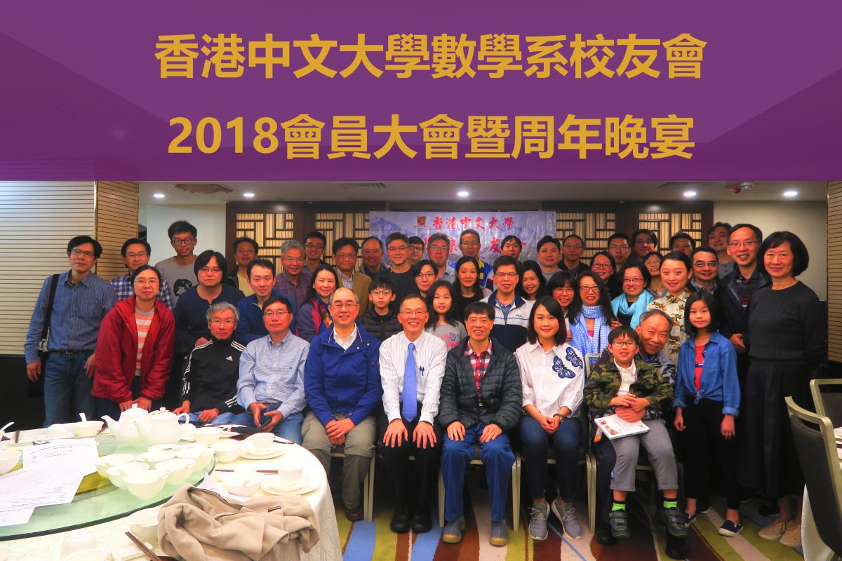
時光荏苒,不經不覺間,中大數學系已成立了數十個寒暑了!期間數學系人才輩出。2015年,在數學系系主任陳漢夫教授的大力推動、支持及一眾校友見證下,「香港中文大學數學系校友會」(CUHK Mathematics Alumni Association) 正式成立,校友會宗旨是:加強會員之關係及團結,促進會員福利及協助中大數學系之發展。本會會章可參閱[此頁](/people/alumni/alumni-association/constitution)
。2018-19屆幹事會有職守理事如下:
會 長: 龍德義 (84新亞)
副會長: 王華峰 (94新亞)
秘 書: 李 星 (07逸夫)
財 政: 張亮夫 (82新亞)
推 廣: 劉仲強 (12聯合)
幹 事: 梁玉明 (94新亞)
* * *
#### 2018年會員大會暨周年聚餐
各位校友︰
大家好!校友會即將舉辦2018年會員大會暨周年聚餐,誠邀各位校友出席。活動資料如下︰
日期:2018年3月24日(星期六)
時間:下午六時三十分
地點:中大崇基學院教職員聯誼會會所 (品御軒)
費用:$250 (費用請於當晚將款項交予本會幹事,一經報名便作實論。如當晚未能出席,$250款項亦必須交予本會幹事)
\*\*餐廳附近有少量泊車位。如果閣下當日需要泊車,可於報名時將車牌號碼一併電郵至本會([cumaa@math.cuhk.edu.hk](mailto:cumaa@math.cuhk.edu.hk)
),本會將以先到先得方式安排中大泊車券予閣下。
如欲報名參加是次會員大會暨周年聚餐,請填寫下列資料,並於3月10日前電郵至本會,謝謝!
姓 名:
聯絡電話:
電 郵:
畢業年份:
修讀課程:
所屬書院(如適用):
車牌號碼(如需要中大泊車券):
聚餐當晚亦會舉行會員大會及幹事會選舉。如閣下有意提名會員出任幹事會,或未能出席會員大會而希望投票權由其他出席的校友代行,歡迎經電郵向我們索取相關文件。謝謝。
歡迎各位約定好友,在當晚共敘同窗深情!為免向隅,報名從速。如有任何查詢,歡迎電郵至 [cumaa@math.cuhk.edu.hk](mailto:cumaa@math.cuhk.edu.hk)
聯絡我們。
香港中文大學數學系校友會幹事會 謹啟
<[cumaa@math.cuhk.edu.hk](mailto:cumaa@math.cuhk.edu.hk)
\>
「香港中文大學數學系校友會」(CUHK Mathematics Alumni Association)
* * *
#### Graduation Greetings from CUMAA to all Year 4 Mathematics Students (2017)
Dear all Year 4 Mathematics Students,
Time flies. I think all of you are heavily involving in preparing for your forthcoming final examination. On behalf of the CUHK Mathematics Alumni Association (CUMAA), I would like to take this opportunity to wish you every smooth and success in the examination. And of course, I would like to say in advance to congratulate you the graduation in advance.
For the time being, you are cordially invited to join the CUMAA. The aims of the Association are to foster alumni’s effort and strengths to match with our Department’s current direction of the development to continuously support Mathematics development in Hong Kong and keep on contributing to it.
For the way to join our “Big Family” or contact us, you may refer to the following
* Website:
* [http://www.math.cuhk.edu.hk/people/alumni/alumni-association](http://www.math.cuhk.edu.hk/people/alumni/alumni-association)
* Email:
* [cumaa@math.cuhk.edu.hk](mailto:cumaa@math.cuhk.edu.hk)
* Contact Point:
* Dr LEUNG King-man (President of CUMAA) Tel : 94853210
* Dr CHEUNG Leung-fu (Treasury of CUMAA) Tel : 39437961
Once again, may I welcome you all and wish to see you in our forthcoming events or activities.
Keep in touch.
Finally, wishing all of you good health, lots of unforgettable moment on the campus and enjoyable study in the Mathematics Department.
Best regards
Dr KM LEUNG
for the Executive Committee of CUMAA
(香港中文大學數學系校友會會長梁敬文博士暨全體幹事謹上)
April 2017
* * *
[「香港中文大學數學系校友會」第 二屆會員大會暨周年聚餐 相片分享](/people/alumni/alumni-association/photo-gallery#20170306)
* * *
#### 第二屆會員大會暨週年聚餐
各位校友,
又是一年辭舊迎新的時刻,校友會幹事會祝大家在新的一年裏,身體健康,萬事如意,花開富貴,心中有數!
校友會誠邀你出席
第二屆會員大會暨週年聚餐
日期: 2017年3月4日(星期六)
時間: 下午六時三十分
地點: \[更新\] 和聲滬軒 (中大和聲書院低層二樓)
費用:$200 (費用請於當晚將款項交予本會幹事,一經報名便作實論。)
\*\*\*\*\*\*\*\*\*\*\*\*\*\*\*\*\*\*\*\*\*\*\*\*\*\*\*\*\*\*\*\*\*\*\*\*\*\*\*\*\*\*\*\*\*\*\*\*\*\*\*\*\*\*\*\*\*\*\*\*\*\*\*\*\*\*\*\*\*\*\*\*\*\*\*\*\*\*\*\*
已確定出席之教職員:陳漢夫教授 譚炳均博士 名單不斷更新中
\*\*\*\*\*\*\*\*\*\*\*\*\*\*\*\*\*\*\*\*\*\*\*\*\*\*\*\*\*\*\*\*\*\*\*\*\*\*\*\*\*\*\*\*\*\*\*\*\*\*\*\*\*\*\*\*\*\*\*\*\*\*\*\*\*\*\*\*\*\*\*\*\*\*\*\*\*\*\*\*
是晚節目內容豐富:嘉賓分享,會務報告,趣味問答,幸運抽獎...... 當晚出席之校友會會員更可獲贈系紙一疊,非會員可即場入會
報名參加會員大會暨周年聚餐方法,請填寫下列資料,並於3月1日前電郵給我們 ([cumaa@math.cuhk.edu.hk](mailto:cumaa@math.cuhk.edu.hk)
)。
姓 名:
聯絡電話:
電 郵:
畢業年份:
修讀課程:
所屬書院(如適用):
\*\*\*\*\*\*\*\*\*\*\*\*\*\*\*\*\*\*\*\*\*\*\*\*\*\*\*\*\*\*\*\*\*\*\*\*\*\*\*\*\*\*\*\*\*\*\*\*\*\*\*\*\*\*\*\*\*\*\*\*\*\*\*\*\*\*\*\*\*\*\*\*\*\*\*\*\*\*\*\*
約定舊時好友,共敘同窗深情! 為免向隅,報名從速
如有任何查詢,請電郵 [.hk](mailto:cumaa@math.cuhk.edu.hk)
聯絡我們。
香港中文大學數學系校友會首屆幹事會
會 長: 梁敬文 (86新亞)
副會長: 劉仲强 (12聯合)
秘 書: 李 星 (07逸夫)
財 政: 張亮夫 (82新亞)
推 廣: 王華峰 (94新亞)
幹 事: 陳彩珍 (92聯合)、陳美珊 (99崇基)
謹啟
* * *
#### 11月校友會活動︰遠足(梅子林到馬鞍山昂平)
本會將於本年11月27日早上舉辦遠足活動,希望讓大家在秋季一起親親大自然,與其他校友共聚、交流。請各位興趣參加的校友踴躍報名!
| | |
| --- | --- |
| 日期 | 2016年11月27日 (星期日) |
| 時間 | 09:00 ~ 14:00 |
| 集合時間 | 09:00 |
| 集合地點 | 港鐵大水坑站大堂 |
| 行程 | 大水坑站 => 梅子林 => 茅坪 => 昂平 => 馬鞍山村,全長約8.5km |
| 終點交通 | 到達馬鞍山村後,乘搭村巴84R 到港鐵馬鞍山站 |
| 報名方法 | 請按[https://docs.google.com/forms/d/e/1FAIpQLSeLzKx\_y1\_fdoJEgS\-jdogEERsFfZcHS077lTKsmZaj0uVBgA/viewform](https://docs.google.com/forms/d/e/1FAIpQLSeLzKx_y1_fdoJEgS-jdogEERsFfZcHS077lTKsmZaj0uVBgA/viewform)
填寫資料 |
| 簡介 | 全程有上坡路及下坡路各一段,均屬易行的山徑及車路,而昂平觀景開揚,可以俯瞰西貢及其對開海域的各個小島。 |
| 費用 | 免費 |
| 名額 | 30人 |
| 截止日期 | 2016年 11 月 19 日 |
| 聯絡人 | 劉仲強
電郵︰[cumaa@math.cuhk.edu.hk](mailto:cumaa@math.cuhk.edu.hk) |
| 參考 | [http://www.lcsd.gov.hk/tc/healthy/hiking/road\_nature/road\_nature5.html#](http://www.lcsd.gov.hk/tc/healthy/hiking/road_nature/road_nature5.html#)
(是次遠足路線與網址中的相同但方向相反) |
| 詳情 | 請按入[https://docs.google.com/forms/d/1YdxUqe8tGOgWhkoioiceGz2g5Cf9AxwHF1Jd0GqvM6c/prefill](https://docs.google.com/forms/d/1YdxUqe8tGOgWhkoioiceGz2g5Cf9AxwHF1Jd0GqvM6c/prefill) |
* * *
#### 數學系校友會致四年級同學的祝賀信
致 中大數學系四年級同學:
首先代表中大數學系校友會(CUMAA)預祝大家考試如意、順利畢業!
再誠意邀請你加入校友會,凝聚校友力量、加強溝通及配合系內發展,繼續為香港數學發展作出貢獻。
有關加入校友會事宜,與及我們的聯絡方法,可參閱以下資料 :
網址︰[http://www.math.cuhk.edu.hk/people/alumni/alumni-association](http://www.math.cuhk.edu.hk/people/alumni/alumni-association)
電郵︰[cumaa@math.cuhk.edu.hk](mailto:cumaa@math.cuhk.edu.hk)
聯絡︰梁敬文博士(會長) 電話: 94853210 或
張亮夫博士(財政) 電話: 39437961
歡迎大家踴躍參與校友會日後舉辦的各項活動,期待與大家見面,大家保持聯絡。
再次祝大家學業順利、生活愉快、事事如意!
香港中文大學數學系校友會會長梁敬文博士暨全體幹事謹上
二零一六年四月
* * *
[「香港中文大學數學系校友會」第一屆會員大會暨周年聚餐 相片分享 及 校友曹啟昇教授「七律」來鴻](/people/alumni/alumni-association/photo-gallery#20160312)
* * *
#### 第一屆會員大會暨周年聚餐
詳情如下
日期: 2016年3月12日(星期六)
時間: 下午六時三十分
地點: 中大崇基學院教職員聯誼會
聚餐費用:$250 (費用請於當晚將款項交予本會幹事,一經報名便作實論。)
報名參加會員大會暨周年聚餐方法,請填寫下列資料,並於三月八日前電郵給我們 ([cumaa@math.cuhk.edu.hk](mailto:cumaa@math.cuhk.edu.hk)
)。
姓 名: 例︰梁某某
聯絡電話: 例︰9xx532x0
電 郵: 例︰[cumaa@math.cuhk.edu.hk](mailto:cumaa@math.cuhk.edu.hk)
畢業年份: 例︰1986
修讀課程: 例︰BSc(Hon)
所屬書院: 例︰NA College
約定你,到時見。如有任何查詢,亦可透過電郵 [cumaa@math.cuhk.edu.hk](mailto:cumaa@math.cuhk.edu.hk)
聯絡我們。
---
# Photo Gallery | CUHK Mathematics
[Skip to main content](#main-content)
[](http://www.cuhk.edu.hk "The Chinese University of Hong Kong")
[](http://www.sci.cuhk.edu.hk/ "Faculty of Science")
[](/ "Home")
Search form
-----------
Search Search Search
[](https://imap.math.cuhk.edu.hk "Math Webmail")
[](/user "Login to this Math Web")
1. [Home](/)
2. [People](/people)
3. [Alumni](/people/alumni)
4. [Alumni Association](/people/alumni/alumni-association)
5. Photo Gallery
Photo Gallery
=============
#### 西貢行山
2018年11月25日
數學系校友會在2018年11月25日成功舉辦了登山活動,往破邊洲觀賞六角石柱奇觀。
[](/sites/default/files/people/alumni-association/gallery/20181125/0A957CA6-557F-441B-ABEC-71DB36479189.jpg "西貢行山")
[](/sites/default/files/people/alumni-association/gallery/20181125/2A59F218-7F4A-4A33-BB21-B2547EB9253C.jpg "西貢行山")
[](/sites/default/files/people/alumni-association/gallery/20181125/BF1D7866-548A-45AB-AB4A-39E45B0976EA.jpg "西貢行山")
[](/sites/default/files/people/alumni-association/gallery/20181125/DSC04664.jpg "西貢行山")
[](/sites/default/files/people/alumni-association/gallery/20181125/DSC04674.jpg "西貢行山")
[](/sites/default/files/people/alumni-association/gallery/20181125/DSC04692.jpg "西貢行山")
[](/sites/default/files/people/alumni-association/gallery/20181125/DSC04708.jpg "西貢行山")
[](/sites/default/files/people/alumni-association/gallery/20181125/DSC04711.jpg "西貢行山")
[](/sites/default/files/people/alumni-association/gallery/20181125/DSC04713.jpg "西貢行山")
[](/sites/default/files/people/alumni-association/gallery/20181125/E08C3F04-CF7B-4790-9FB9-BFEFD7AB321C.jpg "西貢行山")
[](/sites/default/files/people/alumni-association/gallery/20181125/IMG_9880.jpg "西貢行山")
[](/sites/default/files/people/alumni-association/gallery/20181125/IMG_9881.jpg "西貢行山")
[](/sites/default/files/people/alumni-association/gallery/20181125/IMG_9895.jpg "西貢行山")
[](/sites/default/files/people/alumni-association/gallery/20181125/IMG_9905.jpg "西貢行山")
[](/sites/default/files/people/alumni-association/gallery/20181125/IMG_9909.jpg "西貢行山")
[](/sites/default/files/people/alumni-association/gallery/20181125/IMG_20181125_092147.jpg "西貢行山")
[](/sites/default/files/people/alumni-association/gallery/20181125/IMG_20181125_092247.jpg "西貢行山")
[](/sites/default/files/people/alumni-association/gallery/20181125/IMG_20181125_095604.jpg "西貢行山")
[](/sites/default/files/people/alumni-association/gallery/20181125/IMG_20181125_104058.jpg "西貢行山")
[](/sites/default/files/people/alumni-association/gallery/20181125/IMG_20181125_104216.jpg "西貢行山")
[](/sites/default/files/people/alumni-association/gallery/20181125/IMG_20181125_111307_1.jpg "西貢行山")
[](/sites/default/files/people/alumni-association/gallery/20181125/IMG_20181125_115456.jpg "西貢行山")
[](/sites/default/files/people/alumni-association/gallery/20181125/IMG_20181125_115503.jpg "西貢行山")
* * *
#### 中大校友日
2018年11月24日
數學系校友會在2018年11月24日首次於中大校友日設立遊戲攤位,與一衆校友、家屬感受拼砌七巧板的樂趣。
[](/sites/default/files/people/alumni-association/gallery/20181124/IMG_20181124_113609.jpg "中大校友日")
[](/sites/default/files/people/alumni-association/gallery/20181124/IMG_20181124_114042.jpg "中大校友日")
[](/sites/default/files/people/alumni-association/gallery/20181124/IMG_20181124_114431.jpg "中大校友日")
[](/sites/default/files/people/alumni-association/gallery/20181124/IMG_20181124_114519.jpg "中大校友日")
[](/sites/default/files/people/alumni-association/gallery/20181124/IMG_20181124_114726.jpg "中大校友日")
[](/sites/default/files/people/alumni-association/gallery/20181124/IMG_20181124_115428.jpg "中大校友日")
[](/sites/default/files/people/alumni-association/gallery/20181124/IMG_20181124_115436.jpg "中大校友日")
[](/sites/default/files/people/alumni-association/gallery/20181124/IMG_20181124_120424.jpg "中大校友日")
[](/sites/default/files/people/alumni-association/gallery/20181124/IMG_20181124_120435.jpg "中大校友日")
[](/sites/default/files/people/alumni-association/gallery/20181124/IMG_20181124_130714.jpg "中大校友日")
[](/sites/default/files/people/alumni-association/gallery/20181124/IMG_20181124_142625.jpg "中大校友日")
[](/sites/default/files/people/alumni-association/gallery/20181124/IMG_20181124_142625_1.jpg "中大校友日")
[](/sites/default/files/people/alumni-association/gallery/20181124/IMG_20181124_145241.jpg "中大校友日")
[](/sites/default/files/people/alumni-association/gallery/20181124/IMG_20181124_145339.jpg "中大校友日")
* * *
#### 2018年會員大會暨周年聚餐 相片分享
2018年3月24日
[](http://www.math.cuhk.edu.hk/sites/default/files/people/alumni-association/gallery/20180324/img_7005.jpg "2018年會員大會暨周年聚餐 相片分享")
[](http://www.math.cuhk.edu.hk/sites/default/files/people/alumni-association/gallery/20180324/img_7016.jpg "2018年會員大會暨周年聚餐 相片分享")
[](http://www.math.cuhk.edu.hk/sites/default/files/people/alumni-association/gallery/20180324/img_7026.jpg "2018年會員大會暨周年聚餐 相片分享")
[](http://www.math.cuhk.edu.hk/sites/default/files/people/alumni-association/gallery/20180324/img_7040.jpg "2018年會員大會暨周年聚餐 相片分享")
[](http://www.math.cuhk.edu.hk/sites/default/files/people/alumni-association/gallery/20180324/img_7045.jpg "2018年會員大會暨周年聚餐 相片分享")
[](http://www.math.cuhk.edu.hk/sites/default/files/people/alumni-association/gallery/20180324/img_7049.jpg "2018年會員大會暨周年聚餐 相片分享")
[](http://www.math.cuhk.edu.hk/sites/default/files/people/alumni-association/gallery/20180324/0cimg9706.jpg "2018年會員大會暨周年聚餐 相片分享")
[](http://www.math.cuhk.edu.hk/sites/default/files/people/alumni-association/gallery/20180324/002.jpg "2018年會員大會暨周年聚餐 相片分享")
[](http://www.math.cuhk.edu.hk/sites/default/files/people/alumni-association/gallery/20180324/003.jpg "2018年會員大會暨周年聚餐 相片分享")
[](http://www.math.cuhk.edu.hk/sites/default/files/people/alumni-association/gallery/20180324/004.jpg "2018年會員大會暨周年聚餐 相片分享")
[](http://www.math.cuhk.edu.hk/sites/default/files/people/alumni-association/gallery/20180324/005.jpg "2018年會員大會暨周年聚餐 相片分享")
[](http://www.math.cuhk.edu.hk/sites/default/files/people/alumni-association/gallery/20180324/006.jpg "2018年會員大會暨周年聚餐 相片分享")
[](http://www.math.cuhk.edu.hk/sites/default/files/people/alumni-association/gallery/20180324/007.jpg "2018年會員大會暨周年聚餐 相片分享")
[](http://www.math.cuhk.edu.hk/sites/default/files/people/alumni-association/gallery/20180324/008.jpg "2018年會員大會暨周年聚餐 相片分享")
[](http://www.math.cuhk.edu.hk/sites/default/files/people/alumni-association/gallery/20180324/009.jpg "2018年會員大會暨周年聚餐 相片分享")
[](http://www.math.cuhk.edu.hk/sites/default/files/people/alumni-association/gallery/20180324/010.jpg "2018年會員大會暨周年聚餐 相片分享")
[](http://www.math.cuhk.edu.hk/sites/default/files/people/alumni-association/gallery/20180324/011.jpg "2018年會員大會暨周年聚餐 相片分享")
[](http://www.math.cuhk.edu.hk/sites/default/files/people/alumni-association/gallery/20180324/012.jpg "2018年會員大會暨周年聚餐 相片分享")
[](http://www.math.cuhk.edu.hk/sites/default/files/people/alumni-association/gallery/20180324/013.jpg "2018年會員大會暨周年聚餐 相片分享")
[](http://www.math.cuhk.edu.hk/sites/default/files/people/alumni-association/gallery/20180324/014.jpg "2018年會員大會暨周年聚餐 相片分享")
[](http://www.math.cuhk.edu.hk/sites/default/files/people/alumni-association/gallery/20180324/015.jpg "2018年會員大會暨周年聚餐 相片分享")
[](http://www.math.cuhk.edu.hk/sites/default/files/people/alumni-association/gallery/20180324/016.jpg "2018年會員大會暨周年聚餐 相片分享")
[](http://www.math.cuhk.edu.hk/sites/default/files/people/alumni-association/gallery/20180324/017.jpg "2018年會員大會暨周年聚餐 相片分享")
[](http://www.math.cuhk.edu.hk/sites/default/files/people/alumni-association/gallery/20180324/018.jpg "2018年會員大會暨周年聚餐 相片分享")
[](http://www.math.cuhk.edu.hk/sites/default/files/people/alumni-association/gallery/20180324/019.jpg "2018年會員大會暨周年聚餐 相片分享")
[](http://www.math.cuhk.edu.hk/sites/default/files/people/alumni-association/gallery/20180324/020.jpg "2018年會員大會暨周年聚餐 相片分享")
[](http://www.math.cuhk.edu.hk/sites/default/files/people/alumni-association/gallery/20180324/021.jpg "2018年會員大會暨周年聚餐 相片分享")
[](http://www.math.cuhk.edu.hk/sites/default/files/people/alumni-association/gallery/20180324/022.jpg "2018年會員大會暨周年聚餐 相片分享")
[](http://www.math.cuhk.edu.hk/sites/default/files/people/alumni-association/gallery/20180324/023.jpg "2018年會員大會暨周年聚餐 相片分享")
[](http://www.math.cuhk.edu.hk/sites/default/files/people/alumni-association/gallery/20180324/024.jpg "2018年會員大會暨周年聚餐 相片分享")
[](http://www.math.cuhk.edu.hk/sites/default/files/people/alumni-association/gallery/20180324/025.jpg "2018年會員大會暨周年聚餐 相片分享")
[](http://www.math.cuhk.edu.hk/sites/default/files/people/alumni-association/gallery/20180324/026.jpg "2018年會員大會暨周年聚餐 相片分享")
[](http://www.math.cuhk.edu.hk/sites/default/files/people/alumni-association/gallery/20180324/cimg9730.jpg "2018年會員大會暨周年聚餐 相片分享")
[](http://www.math.cuhk.edu.hk/sites/default/files/people/alumni-association/gallery/20180324/cimg9734.jpg "2018年會員大會暨周年聚餐 相片分享")
[](http://www.math.cuhk.edu.hk/sites/default/files/people/alumni-association/gallery/20180324/cimg9736.jpg "2018年會員大會暨周年聚餐 相片分享")
[](http://www.math.cuhk.edu.hk/sites/default/files/people/alumni-association/gallery/20180324/cimg9739.jpg "2018年會員大會暨周年聚餐 相片分享")
[](http://www.math.cuhk.edu.hk/sites/default/files/people/alumni-association/gallery/20180324/cimg9760.jpg "2018年會員大會暨周年聚餐 相片分享")
* * *
#### 第二屆會員大會暨周年聚餐 相片分享
2017年3月4日
[](http://www.math.cuhk.edu.hk/sites/default/files/people/alumni-association/gallery/20170306/cimg8914.jpg "第二屆會員大會暨周年聚餐")
[](http://www.math.cuhk.edu.hk/sites/default/files/people/alumni-association/gallery/20170306/cimg8915.jpg "第二屆會員大會暨周年聚餐")
[](http://www.math.cuhk.edu.hk/sites/default/files/people/alumni-association/gallery/20170306/cimg8917.jpg "第二屆會員大會暨周年聚餐")
[](http://www.math.cuhk.edu.hk/sites/default/files/people/alumni-association/gallery/20170306/cimg8918.jpg "第二屆會員大會暨周年聚餐")
[](http://www.math.cuhk.edu.hk/sites/default/files/people/alumni-association/gallery/20170306/cimg8922.jpg "第二屆會員大會暨周年聚餐")
[](http://www.math.cuhk.edu.hk/sites/default/files/people/alumni-association/gallery/20170306/cimg8924.jpg "第二屆會員大會暨周年聚餐")
[](http://www.math.cuhk.edu.hk/sites/default/files/people/alumni-association/gallery/20170306/cimg8925.jpg "第二屆會員大會暨周年聚餐")
[](http://www.math.cuhk.edu.hk/sites/default/files/people/alumni-association/gallery/20170306/cimg8926.jpg "第二屆會員大會暨周年聚餐")
[](http://www.math.cuhk.edu.hk/sites/default/files/people/alumni-association/gallery/20170306/cimg8927.jpg "第二屆會員大會暨周年聚餐")
[](http://www.math.cuhk.edu.hk/sites/default/files/people/alumni-association/gallery/20170306/cimg8937.jpg "第二屆會員大會暨周年聚餐")
[](http://www.math.cuhk.edu.hk/sites/default/files/people/alumni-association/gallery/20170306/cimg8942.jpg "第二屆會員大會暨周年聚餐")
[](http://www.math.cuhk.edu.hk/sites/default/files/people/alumni-association/gallery/20170306/cimg8952.jpg "第二屆會員大會暨周年聚餐")
[](http://www.math.cuhk.edu.hk/sites/default/files/people/alumni-association/gallery/20170306/cimg8958.jpg "第二屆會員大會暨周年聚餐")
[](http://www.math.cuhk.edu.hk/sites/default/files/people/alumni-association/gallery/20170306/cimg8972.jpg "第二屆會員大會暨周年聚餐")
[](http://www.math.cuhk.edu.hk/sites/default/files/people/alumni-association/gallery/20170306/cimg8975.jpg "第二屆會員大會暨周年聚餐")
[](http://www.math.cuhk.edu.hk/sites/default/files/people/alumni-association/gallery/20170306/cimg8977.jpg "第二屆會員大會暨周年聚餐")
[](http://www.math.cuhk.edu.hk/sites/default/files/people/alumni-association/gallery/20170306/cimg8979.jpg "第二屆會員大會暨周年聚餐")
[](http://www.math.cuhk.edu.hk/sites/default/files/people/alumni-association/gallery/20170306/cimg8981.jpg "第二屆會員大會暨周年聚餐")
[](http://www.math.cuhk.edu.hk/sites/default/files/people/alumni-association/gallery/20170306/cimg8984.jpg "第二屆會員大會暨周年聚餐")
[](http://www.math.cuhk.edu.hk/sites/default/files/people/alumni-association/gallery/20170306/cimg8985.jpg "第二屆會員大會暨周年聚餐")
[](http://www.math.cuhk.edu.hk/sites/default/files/people/alumni-association/gallery/20170306/cimg8988.jpg "第二屆會員大會暨周年聚餐")
[](http://www.math.cuhk.edu.hk/sites/default/files/people/alumni-association/gallery/20170306/cimg8990.jpg "第二屆會員大會暨周年聚餐")
[](http://www.math.cuhk.edu.hk/sites/default/files/people/alumni-association/gallery/20170306/cimg8992.jpg "第二屆會員大會暨周年聚餐")
[](http://www.math.cuhk.edu.hk/sites/default/files/people/alumni-association/gallery/20170306/cimg8993.jpg "第二屆會員大會暨周年聚餐")
[](http://www.math.cuhk.edu.hk/sites/default/files/people/alumni-association/gallery/20170306/cimg8994.jpg "第二屆會員大會暨周年聚餐")
[](http://www.math.cuhk.edu.hk/sites/default/files/people/alumni-association/gallery/20170306/cimg8997.jpg "第二屆會員大會暨周年聚餐")
[](http://www.math.cuhk.edu.hk/sites/default/files/people/alumni-association/gallery/20170306/cimg8999.jpg "第二屆會員大會暨周年聚餐")
[](http://www.math.cuhk.edu.hk/sites/default/files/people/alumni-association/gallery/20170306/cimg9001.jpg "第二屆會員大會暨周年聚餐")
[](http://www.math.cuhk.edu.hk/sites/default/files/people/alumni-association/gallery/20170306/cimg9003.jpg "第二屆會員大會暨周年聚餐")
[](http://www.math.cuhk.edu.hk/sites/default/files/people/alumni-association/gallery/20170306/cimg9004.jpg "第二屆會員大會暨周年聚餐")
[](http://www.math.cuhk.edu.hk/sites/default/files/people/alumni-association/gallery/20170306/cimg9006.jpg "第二屆會員大會暨周年聚餐")
[](http://www.math.cuhk.edu.hk/sites/default/files/people/alumni-association/gallery/20170306/cimg9008.jpg "第二屆會員大會暨周年聚餐")
[](http://www.math.cuhk.edu.hk/sites/default/files/people/alumni-association/gallery/20170306/cimg9009.jpg "第二屆會員大會暨周年聚餐")
[](http://www.math.cuhk.edu.hk/sites/default/files/people/alumni-association/gallery/20170306/cimg9011.jpg "第二屆會員大會暨周年聚餐")
[](http://www.math.cuhk.edu.hk/sites/default/files/people/alumni-association/gallery/20170306/cimg9012.jpg "第二屆會員大會暨周年聚餐")
[](http://www.math.cuhk.edu.hk/sites/default/files/people/alumni-association/gallery/20170306/dsc_0677_1.jpg "第二屆會員大會暨周年聚餐")
[](http://www.math.cuhk.edu.hk/sites/default/files/people/alumni-association/gallery/20170306/dsc_0681.jpg "第二屆會員大會暨周年聚餐")
[](http://www.math.cuhk.edu.hk/sites/default/files/people/alumni-association/gallery/20170306/dsc_0682.jpg "第二屆會員大會暨周年聚餐")
[](http://www.math.cuhk.edu.hk/sites/default/files/people/alumni-association/gallery/20170306/dsc_0683.jpg "第二屆會員大會暨周年聚餐")
[](http://www.math.cuhk.edu.hk/sites/default/files/people/alumni-association/gallery/20170306/dsc_0687.jpg "第二屆會員大會暨周年聚餐")
[](http://www.math.cuhk.edu.hk/sites/default/files/people/alumni-association/gallery/20170306/dsc_0693.jpg "第二屆會員大會暨周年聚餐")
[](http://www.math.cuhk.edu.hk/sites/default/files/people/alumni-association/gallery/20170306/dsc_0695.jpg "第二屆會員大會暨周年聚餐")
[](http://www.math.cuhk.edu.hk/sites/default/files/people/alumni-association/gallery/20170306/dsc_0696.jpg "第二屆會員大會暨周年聚餐")
[](http://www.math.cuhk.edu.hk/sites/default/files/people/alumni-association/gallery/20170306/dsc_0699_2.jpg "第二屆會員大會暨周年聚餐")
[](http://www.math.cuhk.edu.hk/sites/default/files/people/alumni-association/gallery/20170306/img_2845.jpg "第二屆會員大會暨周年聚餐")
[](http://www.math.cuhk.edu.hk/sites/default/files/people/alumni-association/gallery/20170306/img_2907.jpg "第二屆會員大會暨周年聚餐")
[](http://www.math.cuhk.edu.hk/sites/default/files/people/alumni-association/gallery/20170306/img_2908.jpg "第二屆會員大會暨周年聚餐")
[](http://www.math.cuhk.edu.hk/sites/default/files/people/alumni-association/gallery/20170306/img_2909.jpg "第二屆會員大會暨周年聚餐")
[](http://www.math.cuhk.edu.hk/sites/default/files/people/alumni-association/gallery/20170306/img_2910.jpg "第二屆會員大會暨周年聚餐")
[](http://www.math.cuhk.edu.hk/sites/default/files/people/alumni-association/gallery/20170306/p1010187.jpg "第二屆會員大會暨周年聚餐")
[](http://www.math.cuhk.edu.hk/sites/default/files/people/alumni-association/gallery/20170306/p1010200.jpg "第二屆會員大會暨周年聚餐")
[](http://www.math.cuhk.edu.hk/sites/default/files/people/alumni-association/gallery/20170306/p1010211.jpg "第二屆會員大會暨周年聚餐")
[](http://www.math.cuhk.edu.hk/sites/default/files/people/alumni-association/gallery/20170306/p1010212.jpg "第二屆會員大會暨周年聚餐")
[](http://www.math.cuhk.edu.hk/sites/default/files/people/alumni-association/gallery/20170306/p1010214.jpg "第二屆會員大會暨周年聚餐")
[](http://www.math.cuhk.edu.hk/sites/default/files/people/alumni-association/gallery/20170306/p1010217.jpg "第二屆會員大會暨周年聚餐")
[](http://www.math.cuhk.edu.hk/sites/default/files/people/alumni-association/gallery/20170306/p1010220.jpg "第二屆會員大會暨周年聚餐")
[](http://www.math.cuhk.edu.hk/sites/default/files/people/alumni-association/gallery/20170306/p1010229.jpg "第二屆會員大會暨周年聚餐")
[](http://www.math.cuhk.edu.hk/sites/default/files/people/alumni-association/gallery/20170306/p1010248.jpg "第二屆會員大會暨周年聚餐")
[](http://www.math.cuhk.edu.hk/sites/default/files/people/alumni-association/gallery/20170306/p1010250.jpg "第二屆會員大會暨周年聚餐")
[](http://www.math.cuhk.edu.hk/sites/default/files/people/alumni-association/gallery/20170306/p1010259.jpg "第二屆會員大會暨周年聚餐")
* * *
#### 第一屆會員大會暨周年聚餐 相片分享 及 校友曹啟昇教授「七律」來鴻
2016年3月12日
《數 學 校 友 會 晚 宴》 曹 啟 昇
疇 學 元 來 國 棟 梁,矩 窺 天 道 發 幽 光。
歌 弦 數 載 同 風 雨,絕 足 無 垠 任 雪 霜。
春 宴 華 堂 寒 料 峭,蒼 顏 綠 鬢 意 昂 揚。
歡 會 明 年 應 更 勝,香 茶 代 酒 各 傾 觴。
[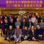](http://www.math.cuhk.edu.hk/sites/default/files/people/alumni-association/gallery/20160312/1cumaadinner2016.jpg "第一屆會員大會暨周年聚餐")
[](http://www.math.cuhk.edu.hk/sites/default/files/people/alumni-association/gallery/20160312/cimg7977.jpg "第一屆會員大會暨周年聚餐")
[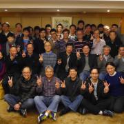](http://www.math.cuhk.edu.hk/sites/default/files/people/alumni-association/gallery/20160312/p1070639.jpg "第一屆會員大會暨周年聚餐")
[](http://www.math.cuhk.edu.hk/sites/default/files/people/alumni-association/gallery/20160312/p1070645.jpg "第一屆會員大會暨周年聚餐")
[](http://www.math.cuhk.edu.hk/sites/default/files/people/alumni-association/gallery/20160312/p1070695.jpg "第一屆會員大會暨周年聚餐")
[](http://www.math.cuhk.edu.hk/sites/default/files/people/alumni-association/gallery/20160312/p1070700.jpg "第一屆會員大會暨周年聚餐")
[](http://www.math.cuhk.edu.hk/sites/default/files/people/alumni-association/gallery/20160312/p1070726.jpg "第一屆會員大會暨周年聚餐")
[](http://www.math.cuhk.edu.hk/sites/default/files/people/alumni-association/gallery/20160312/p1070735.jpg "第一屆會員大會暨周年聚餐")
[](http://www.math.cuhk.edu.hk/sites/default/files/people/alumni-association/gallery/20160312/p1070755.jpg "第一屆會員大會暨周年聚餐")
[](http://www.math.cuhk.edu.hk/sites/default/files/people/alumni-association/gallery/20160312/p1070761.jpg "第一屆會員大會暨周年聚餐")
[](http://www.math.cuhk.edu.hk/sites/default/files/people/alumni-association/gallery/20160312/p1070767.jpg "第一屆會員大會暨周年聚餐")
[](http://www.math.cuhk.edu.hk/sites/default/files/people/alumni-association/gallery/20160312/p1070770.jpg "第一屆會員大會暨周年聚餐")
[](http://www.math.cuhk.edu.hk/sites/default/files/people/alumni-association/gallery/20160312/p1070776.jpg "第一屆會員大會暨周年聚餐")
[](http://www.math.cuhk.edu.hk/sites/default/files/people/alumni-association/gallery/20160312/p1070782.jpg "第一屆會員大會暨周年聚餐")
[](http://www.math.cuhk.edu.hk/sites/default/files/people/alumni-association/gallery/20160312/p1070796.jpg "第一屆會員大會暨周年聚餐")
[](http://www.math.cuhk.edu.hk/sites/default/files/people/alumni-association/gallery/20160312/p1070798.jpg "第一屆會員大會暨周年聚餐")
---
# Research Graduate Students | CUHK Mathematics
[Skip to main content](#main-content)
[](http://www.cuhk.edu.hk "The Chinese University of Hong Kong")
[](http://www.sci.cuhk.edu.hk/ "Faculty of Science")
[](/ "Home")
Search form
-----------
Search Search Search
[](https://imap.math.cuhk.edu.hk "Math Webmail")
[](/user "Login to this Math Web")
1. [Home](/)
2. [People](/people)
3. Research Graduate Students
Research Graduate Students
==========================
_(As of 2024/25 1st Term)_

#### Mr. CHAN Kam Fai Alan
**Program:** Ph.D
**Office:**LSB 232
**Tel:** 3943 5294
**Email:** [akfchan@math.cuhk.edu.hk](mailto:akfchan@math.cuhk.edu.hk)
**Research Interests:** Fluid Dynamics

#### Mr. CHAN Ki Fung
**Program:** Ph.D
**Office:**AB1 505
**Tel:** 3943 4298
**Email:** [kfchan@math.cuhk.edu.hk](mailto:kfchan@math.cuhk.edu.hk)
**Research Interests:** 3d Mirror symmetry, representation theory

#### Mr. CHAN Tsz Hong Clive Junior
**Program:** M.Phil.
**Office:**LSB G05
**Tel:**
**Email:** [thchan@math.cuhk.edu.hk](mailto:thchan@math.cuhk.edu.hk)
**Research Interests:**

#### Mr. CHEN Haiyu
**Program:** Ph.D
**Office:**AB1 614
**Tel:** 3943 4109
**Email:** [hychen@math.cuhk.edu.hk](mailto:hychen@math.cuhk.edu.hk)
**Research Interests:** Lie theory, representation theory

#### Mr. CHEN Meiguang
**Program:** Ph.D
**Office:**AB1 614
**Tel:** 3943 4109
**Email:** [mgchen@math.cuhk.edu.hk](mailto:mgchen@math.cuhk.edu.hk)
**Research Interests:** Partial Differential Equations

#### Mr. CHEN Qiguang
**Program:** Ph.D
**Office:**LSB 222B
**Tel:** 3943 7963
**Email:** [qgchen@math.cuhk.edu.hk](mailto:qgchen@math.cuhk.edu.hk)
**Research Interests:** Quasiconformal geometry and deep learning

#### Mr. CHEN Ruizhe
**Program:** Ph.D.
**Office:**LSB 222C
**Tel:** 3943 8570
**Email:** [rzchen@math.cuhk.edu.hk](mailto:rzchen@math.cuhk.edu.hk)
**Research Interests:**

#### Mr. CHEN Yue
**Program:** M.Phil
**Office:**AB1 407B
**Tel:** 3943 3720
**Email:** [ychen@math.cuhk.edu.hk](mailto:ychen@math.cuhk.edu.hk)
**Research Interests:**

#### Miss CHOW Tsz Ching
**Program:** M.Phil (PT)
**Office:**Sino 540A
**Tel:** 3943 5415
**Email:** [tcchow@math.cuhk.edu.hk](mailto:tcchow@math.cuhk.edu.hk)
**Research Interests:**

#### Mr. CHOY Zi Him Jason
**Program:** Ph.D
**Office:**LSB 222A
**Tel:** 3943 3575
**Email:** [zhchoy@math.cuhk.edu.hk](mailto:zhchoy@math.cuhk.edu.hk)
**Research Interests:**

#### Mr. CUI Han
**Program:** Ph.D
**Office:**AB1 614
**Tel:** 3943 4109
**Email:** [hcui@math.cuhk.edu.hk](mailto:hcui@math.cuhk.edu.hk)
**Research Interests:**

#### Mr. DENG Maolin
**Program:** Ph.D.
**Office:**LSB 222A
**Tel:** 3943 8570
**Email:** [mldeng@math.cuhk.edu.hk](mailto:mldeng@math.cuhk.edu.hk)
**Research Interests:**

#### Mr. DING Zijun
**Program:** Ph.D
**Office:**LSB 222C
**Tel:** 3943 8570
**Email:** [zjding@math.cuhk.edu.hk](mailto:zjding@math.cuhk.edu.hk)
**Research Interests:**

#### Mr. FAN Hongbo
**Program:** Ph.D
**Office:**LSB 222B
**Tel:** 3943 7963
**Email:** [hbfan@math.cuhk.edu.hk](mailto:hbfan@math.cuhk.edu.hk)
**Research Interests:** Quasiconformal Geometry, Deep Learning

#### Ms. FAN Yuxin
**Program:** Ph.D
**Office:**LSB 222A
**Tel:** 3943 3575
**Email:** [yxfan@math.cuhk.edu.hk](mailto:yxfan@math.cuhk.edu.hk)
**Research Interests:**

#### Mr. GU Sixuan
**Program:** M.Phil.
**Office:**AB1 407B
**Tel:** 3943 3720
**Email:** [sxgu@math.cuhk.edu.hk](mailto:sxgu@math.cuhk.edu.hk)
**Research Interests:**

#### Mr. GUO Yuhang
**Program:** M.Phil
**Office:**AB1 407B
**Tel:** 3943 3720
**Email:** [yhguo@math.cuhk.edu.hk](mailto:yhguo@math.cuhk.edu.hk)
**Research Interests:**

#### Mr. HAN Zean
**Program:** M.Phil.
**Office:**LSB G05
**Tel:**
**Email:** [zhan@math.cuhk.edu.hk](mailto:zhan@math.cuhk.edu.hk)
**Research Interests:**

#### Mr. HU Haoqiang
**Program:** M.Phil.
**Office:**AB1 505
**Tel:** 3943 4298
**Email:** [hqhu@math.cuhk.edu.hk](mailto:hqhu@math.cuhk.edu.hk)
**Research Interests:**

#### Ms. HU Shuying
**Program:** Ph.D
**Office:**AB1 614
**Tel:** 3943 4109
**Email:** [syhu@math.cuhk.edu.hk](mailto:syhu@math.cuhk.edu.hk)
**Research Interests:**

#### Mr. HU Tianhao
**Program:** Ph.D
**Office:**LSB 222A
**Tel:** 3943 3575
**Email:** [thhu@math.cuhk.edu.hk](mailto:thhu@math.cuhk.edu.hk)
**Research Interests:**

#### Ms. HUANG Chaoyan
**Program:** Ph.D
**Office:**LSB G08
**Tel:** 3943 7594
**Email:** [cyhuang@math.cuhk.edu.hk](mailto:cyhuang@math.cuhk.edu.hk)
**Research Interests:** Image Processing, Data science, Optimization

#### Mr. HUANG Yanwen
**Program:** M.Phil.
**Office:**SC 333B
**Tel:**
**Email:** [ywhuang@math.cuhk.edu.hk](mailto:ywhuang@math.cuhk.edu.hk)
**Research Interests:**

#### Mr. HUANG Yuchen
**Program:** Ph.D
**Office:**LSB 232
**Tel:** 3943 5294
**Email:** [ychuang@math.cuhk.edu.hk](mailto:ychuang@math.cuhk.edu.hk)
**Research Interests:**

#### Miss IBRAR Nida
**Program:** Ph.D.
**Office:**LSB 222A
**Tel:** 3943 8570
**Email:** [nidaibrar@math.cuhk.edu.hk](mailto:nidaibrar@math.cuhk.edu.hk)
**Research Interests:**

#### Mr. IP Tsz Lok
**Program:** M.Phil.
**Office:**SC 333B
**Tel:**
**Email:** [tlip@math.cuhk.edu.hk](mailto:tlip@math.cuhk.edu.hk)
**Research Interests:**

#### Mr. JIANG Qinghai
**Program:** Ph.D.
**Office:**LSB 222B
**Tel:** 3943 7963
**Email:** [qhjiang@math.cuhk.edu.hk](mailto:qhjiang@math.cuhk.edu.hk)
**Research Interests:**

#### Mr. JIN Chenhan
**Program:** Ph.D (PT)
**Office:**Sino 540A
**Tel:** 3943 5415
**Email:** [chjin2@math.cuhk.edu.hk](mailto:chjin2@math.cuhk.edu.hk)
**Research Interests:**

#### Mr. JIN Xingguang
**Program:** Ph.D
**Office:**LSB 222C
**Tel:** 3943 8570
**Email:** [xgjin@math.cuhk.edu.hk](mailto:xgjin@math.cuhk.edu.hk)
**Research Interests:** Multiscale methods and Deep learning

#### Mr. KANG Jiazhi
**Program:** Ph.D
**Office:**LSB 222B
**Tel:** 3943 7963
**Email:** [jzkang@math.cuhk.edu.hk](mailto:jzkang@math.cuhk.edu.hk)
**Research Interests:** Stochastic Analysis, Stochastic Optimal Control

#### Mr. LAM Chin Hang Eddie
**Program:** Ph.D
**Office:**LSB 222B
**Tel:** 3943 7963
**Email:** [echlam@math.cuhk.edu.hk](mailto:echlam@math.cuhk.edu.hk)
**Research Interests:** Mirror symmetry, symplectic duality

#### Mr. LAN Tianxu
**Program:** Ph.D
**Office:**LSB G08
**Tel:** 3943 7594
**Email:** [txlan@math.cuhk.edu.hk](mailto:txlan@math.cuhk.edu.hk)
**Research Interests:** Stochastic controls and stochastic differential equations

#### Mr. LAU Wing Lim
**Program:** Ph.D.
**Office:**LSB 222C
**Tel:** 3943 8570
**Email:**[](mailto:lwlau@math.cuhk.edu.hk)
**Research Interests:**

#### Mr. LAW Sum Kiu
**Program:** M.Phil.
**Office:**LSB G05
**Tel:**
**Email:** [sklaw@math.cuhk.edu.hk](mailto:sklaw@math.cuhk.edu.hk)
**Research Interests:**

#### Mr. LI Tuoxin
**Program:** Ph.D.
**Office:**LSB 232
**Tel:** 3943 5294
**Email:** [txli@math.cuhk.edu.hk](mailto:txli@math.cuhk.edu.hk)
**Research Interests:**

#### Mr. LI Zeyu
**Program:** Ph.D
**Office:**LSB 222A
**Tel:** 3943 3575
**Email:** [zyli@math.cuhk.edu.hk](mailto:zyli@math.cuhk.edu.hk)
**Research Interests:** Deep learning, Image Process, Optimization

#### Mr. LI Zhiwen
**Program:** Ph.D
**Office:**LSB 222A
**Tel:** 3943 3575
**Email:** [zwli@math.cuhk.edu.hk](mailto:zwli@math.cuhk.edu.hk)
**Research Interests:** Imaging Science, Deep Learning, Scientific Computing

#### Ms. LI Zishang
**Program:** Ph.D
**Office:**LSB 222C
**Tel:** 3943 8570
**Email:** [zsli@math.cuhk.edu.hk](mailto:zsli@math.cuhk.edu.hk)
**Research Interests:** Scientific computing, numerical analysis, multiscale method

#### Mr. LIAO Wenbo
**Program:** Ph.D
**Office:**LSB 232
**Tel:** 3943 5294
**Email:** [wbliao@math.cuhk.edu.hk](mailto:wbliao@math.cuhk.edu.hk)
**Research Interests:**

#### Mr. LIU Ke
**Program:** M.Phil.
**Office:**SC 333B
**Tel:**
**Email:** [kliu@math.cuhk.edu.hk](mailto:kliu@math.cuhk.edu.hk)
**Research Interests:**

#### Mr. LIU Lintao
**Program:** Ph.D.
**Office:**AB1 614
**Tel:** 3943 4109
**Email:** [ltliu@math.cuhk.edu.hk](mailto:ltliu@math.cuhk.edu.hk)
**Research Interests:**

#### Mr. LIU Siqing
**Program:** Ph.D.
**Office:**LSB 222A
**Tel:** 3943 8570
**Email:** [siqingliu@math.cuhk.edu.hk](mailto:siqingliu@math.cuhk.edu.hk)
**Research Interests:**

#### Mr. LIU Sizhe
**Program:** M.Phil.
**Office:**SC 333B
**Tel:**
**Email:** [szliu@math.cuhk.edu.hk](mailto:szliu@math.cuhk.edu.hk)
**Research Interests:**

#### Mr. LIU Yucheng
**Program:** Ph.D
**Office:**LSB 222C
**Tel:** 3943 8570
**Email:** [ycliu@math.cuhk.edu.hk](mailto:ycliu@math.cuhk.edu.hk)
**Research Interests:** Machine learning; Applications of numerical methods

#### Mr. LU Haowen
**Program:** M.Phil
**Office:** AB1 505
**Tel:** 3943 4298
**Email:** [hwlu@math.cuhk.edu.hk](mailto:hwlu@math.cuhk.edu.hk)
**Research Interests:**

#### Mr. LUO Kaihui
**Program:** Ph.D
**Office:**
**Tel:**
**Email:** [khluo@math.cuhk.edu.hk](mailto:khluo@math.cuhk.edu.hk)
**Research Interests:** Free surface problems

#### Mr. LYU Junzhe
**Program:** M.Phil
**Office:**AB1 505
**Tel:** 3943 4298
**Email:** [jzlyu@math.cuhk.edu.hk](mailto:jzlyu@math.cuhk.edu.hk)
**Research Interests:**

#### Mr. MU Zuodong
**Program:** Ph.D
**Office:**LSB 222B
**Tel:** 3943 7963
**Email:** [zdmu@math.cuhk.edu.hk](mailto:zdmu@math.cuhk.edu.hk)
**Research Interests:** Mirror Symmetry and Symplectic Geometry

#### Mr. PAN Zheng
**Program:** Ph.D (PT)
**Office:**
**Tel:**
**Email:** [zpan@math.cuhk.edu.hk](mailto:zpan@math.cuhk.edu.hk)
**Research Interests:**

#### Ms. PANG Xiangying
**Program:** Ph.D
**Office:**LSB 232
**Tel:** 3943 5294
**Email:** [xypang@math.cuhk.edu.hk](mailto:xypang@math.cuhk.edu.hk)
**Research Interests:** Financial Mathematics

#### Mr. PEK Yu-xuan Sean
**Program:** Ph.D
**Office:**LSB 232
**Tel:** 3943 5294
**Email:** [yxpek@math.cuhk.edu.hk](mailto:yxpek@math.cuhk.edu.hk)
**Research Interests:** Representation Theory and Lie Theory

#### Mr. QI Haowei
**Program:** Ph.D.
**Office:**LSB 232
**Tel:** 3943 5294
**Email:** [hwqi@math.cuhk.edu.hk](mailto:hwqi@math.cuhk.edu.hk)
**Research Interests:**

#### Ms. QI Te Jessie
**Program:** Ph.D
**Office:**LSB G08
**Tel:** 3943 37954
**Email:** [tqi@math.cuhk.edu.hk](mailto:tqi@math.cuhk.edu.hk)
**Research Interests:** Image Processing, Optimization, Data Science

#### Mr. SHE Kuigang
**Program:** M.Phil.
**Office:**AB1 407A
**Tel:** 3943 3721
**Email:** [kgshe@math.cuhk.edu.hk](mailto:kgshe@math.cuhk.edu.hk)
**Research Interests:**

#### Mr. SHEN Jianhao
**Program:** Ph.D
**Office:** AB1 614
**Tel:** 3943 4109
**Email:** [jhshen@math.cuhk.edu.hk](mailto:jhshen@math.cuhk.edu.hk)
**Research Interests:** Algebraic number theory, Linear algebraic groups

#### Miss SHEN Yi
**Program:** Ph.D
**Office:** LSB G08
**Tel:** 394335294
**Email:** [yishen@math.cuhk.edu.hk](mailto:yishen@math.cuhk.edu.hk)
**Research Interests:**

#### Mr. SHEN Zhiyuan
**Program:** M.Phil.
**Office:**AB1 505
**Tel:** 3943 4298
**Email:** [zyshen@math.cuhk.edu.hk](mailto:zyshen@math.cuhk.edu.hk)
**Research Interests:**

#### Mr. SHI Linhao
**Program:** Ph.D
**Office:**AB1 614
**Tel:** 3943 4109
**Email:** [lhshi@math.cuhk.edu.hk](mailto:lhshi@math.cuhk.edu.hk)
**Research Interests:** Magnetohydrodynamics PDE; Water waves PDE with free boundary

#### Mr. TIAMIYU Abd'gafar Tunde
**Program:** Ph.D
**Office:**LSB 222C
**Tel:** 3943 8570
**Email:** [tiamiyu@math.cuhk.edu.hk](mailto:tiamiyu@math.cuhk.edu.hk)
**Research Interests:** Inverse problems with deep neural networks and learning theory

#### Mr. TONG Nok To Omega
**Program:** M.Phil.
**Office:**LSB G05
**Tel:**
**Email:** [onttong@math.cuhk.edu.hk](mailto:onttong@math.cuhk.edu.hk)
**Research Interests:**

#### Mr. TSANG Hei Tung
**Program:** M.Phil.
**Office:**SC 333B
**Tel:**
**Email:** [httsang@math.cuhk.edu.hk](mailto:httsang@math.cuhk.edu.hk)
**Research Interests:**

#### Mr. TU Xinyue
**Program:** Ph.D.
**Office:**LSB G05
**Tel:**
**Email:** [xytu@math.cuhk.edu.hk](mailto:xytu@math.cuhk.edu.hk)
**Research Interests:**

#### Mr. Ullah Habib
**Program:** Ph.D
**Office:**LSB 222C
**Tel:** 3943 8570
**Email:** [uhabib@math.cuhk.edu.hk](mailto:uhabib@math.cuhk.edu.hk)
**Research Interests:** Numerical solution of PDE's, Computational fluid dynamics (CFD), Finite element method

#### Mr. WANG Bin
**Program:** Ph.D
**Office:**LSB 222B
**Tel:** 3943 7963
**Email:** [bwang@math.cuhk.edu.hk](mailto:bwang@math.cuhk.edu.hk)
**Research Interests:** Stochastic Analysis and its Applications

#### Miss WANG Hetong
**Program:** Ph.D
**Office:**LSB 232
**Tel:** 3943 5294
**Email:** [htwang@math.cuhk.edu.hk](mailto:htwang@math.cuhk.edu.hk)
**Research Interests:**

#### Mr. WANG Jida
**Program:** M.Phil.
**Office:**SC 333B
**Tel:**
**Email:** [jidawang@math.cuhk.edu.hk](mailto:jidawang@math.cuhk.edu.hk)
**Research Interests:**

#### Mr. WANG Jixin
**Program:** Ph.D
**Office:**LSB 222B
**Tel:** 3943 7963
**Email:** [jxwang@math.cuhk.edu.hk](mailto:jxwang@math.cuhk.edu.hk)
**Research Interests:** Stochastic analysis, Ito's formula

#### Miss WANG Mincheng
**Program:** M.Phil.
**Office:**SC 333B
**Tel:**
**Email:** [mcwang@math.cuhk.edu.hk](mailto:mcwang@math.cuhk.edu.hk)
**Research Interests:**

#### Mr. WANG Ruoyu Steven
**Program:** Ph.D
**Office:**LSB 222B
**Tel:** 3943 7963
**Email:** [rywang@math.cuhk.edu.hk](mailto:rywang@math.cuhk.edu.hk)
**Research Interests:** Quasi-conformal Geometry and Deep Learning

#### Mr. WANG Wenguan
**Program:** Ph.D (PT)
**Office:**
**Tel:**
**Email:** [wgwang@math.cuhk.edu.hk](mailto:wgwang@math.cuhk.edu.hk)
**Research Interests:** Machine Learning and Computer Vision

#### Miss WEI Yulin
**Program:** Ph.D.
**Office:**LSB 222B
**Tel:** 3943 7963
**Email:** [ylwei@math.cuhk.edu.hk](mailto:ylwei@math.cuhk.edu.hk)
**Research Interests:**

#### Mr. WEI Yunsong
**Program:** Ph.D
**Office:**AB1 505
**Tel:** 3943 4298
**Email:** [yswei@math.cuhk.edu.hk](mailto:yswei@math.cuhk.edu.hk)
**Research Interests:** Geometric representation theory, combinatoric algebraic geometry

#### Mr. WU Longjun
**Program:** Ph.D.
**Office:**LSB 222A
**Tel:** 3943 8570
**Email:**[](mailto:ljwu@math.cuhk.edu.hk)
**Research Interests:**

#### Mr. WU Tong
**Program:** M.Phil.
**Office:**LSB G05
**Tel:**
**Email:** [twu@math.cuhk.edu.hk](mailto:twu@math.cuhk.edu.hk)
**Research Interests:**

#### Miss Xia Yu
**Program:** Ph.D.
**Office:**LSB 222A
**Tel:** 3943 8570
**Email:** [yuxia@math.cuhk.edu.hk](mailto:yuxia@math.cuhk.edu.hk)
**Research Interests:**

#### Mr. XIE Yichuan
**Program:** Ph.D.
**Office:**LSB 222A
**Tel:** 3943 8570
**Email:** [ycxie@math.cuhk.edu.hk](mailto:ycxie@math.cuhk.edu.hk)
**Research Interests:**

#### Miss XIONG Wanjun
**Program:** Ph.D.
**Office:**LSB 222A
**Tel:** 3943 8570
**Email:** [wjxiong@math.cuhk.edu.hk](mailto:wjxiong@math.cuhk.edu.hk)
**Research Interests:**

#### Mr. XU Bowei
**Program:** Ph.D
**Office:**LSB 222C
**Tel:** 3943 8570
**Email:** [bwxu@math.cuhk.edu.hk](mailto:bwxu@math.cuhk.edu.hk)
**Research Interests:** Numerical methods and analysis for partial differential equations

#### Mr. XU Jun
**Program:** Ph.D.
**Office:**AB1 407A
**Tel:** 3943 3721
**Email:**[](mailto:jxu@math.cuhk.edu.hk)
**Research Interests:**

#### Mr. XU Shengze
**Program:** Ph.D
**Office:**LSB 222C
**Tel:** 3943 8570
**Email:** [szxu@math.cuhk.edu.hk](mailto:szxu@math.cuhk.edu.hk)
**Research Interests:**

#### Mr. XU Wentao
**Program:** M.Phil
**Office:**AB1 505
**Tel:** 3943 4298
**Email:** [wtxu@math.cuhk.edu.hk](mailto:wtxu@math.cuhk.edu.hk)
**Research Interests:** Algebraic Geometry

#### Mr. XU Zhehao
**Program:** Ph.D
**Office:**LSB 222B
**Tel:** 3943 7963
**Email:** [zhxu@math.cuhk.edu.hk](mailto:zhxu@math.cuhk.edu.hk)
**Research Interests:**

#### Mr. XU Ziyang
**Program:** Ph.D.
**Office:**LSB G08
**Tel:** 3943 7594
**Email:** [zyxu@math.cuhk.edu.hk](mailto:zyxu@math.cuhk.edu.hk)
**Research Interests:**

#### Mr. XUAN Yuanhao
**Program:** Ph.D
**Office:**LSB 222C
**Tel:** 3943 8570
**Email:** [yhxuan@math.cuhk.edu.hk](mailto:yhxuan@math.cuhk.edu.hk)
**Research Interests:**

#### Ms. YANG Anita
**Program:** Ph.D
**Office:**LSB 232
**Tel:** 3943 5294
**Email:** [ayang@math.cuhk.edu.hk](mailto:ayang@math.cuhk.edu.hk)
**Research Interests:** Partial Differential Equations

#### Mr. YANG Bohan
**Program:** Ph.D.
**Office:**LSB 222A
**Tel:** 3943 8570
**Email:** [bhyang@math.cuhk.edu.hk](mailto:bhyang@math.cuhk.edu.hk)
**Research Interests:**

#### Mr. YE Zhenyu
**Program:** M.Phil
**Office:**AB1 505
**Tel:** 3943 4298
**Email:** [zyye@math.cuhk.edu.hk](mailto:zyye@math.cuhk.edu.hk)
**Research Interests:**

#### Mr. YE Zikai
**Program:** Ph.D.
**Office:**LSB 232
**Tel:** 3943 5294
**Email:** [zkye@math.cuhk.edu.hk](mailto:zkye@math.cuhk.edu.hk)
**Research Interests:**

#### Mr. YI Tianhan
**Program:** Ph.D
**Office:**LSB 232
**Tel:** 3943 5294
**Email:** [thyi@math.cuhk.edu.hk](mailto:thyi@math.cuhk.edu.hk)
**Research Interests:** Dynamical System

#### Mr. YU Hang
**Program:** M.Phil.
**Office:**SC 333B
**Tel:**
**Email:** [hyu@math.cuhk.edu.hk](mailto:hyu@math.cuhk.edu.hk)
**Research Interests:**

#### Mr. ZHANG Junhao
**Program:** Ph.D
**Office:**LSB 232
**Tel:** 3943 5294
**Email:** [jhzhang@math.cuhk.edu.hk](mailto:jhzhang@math.cuhk.edu.hk)
**Research Interests:** Nonlinear Partial Differential Equations, Kinetic Theory

#### Miss ZHANG Xinfang
**Program:** M.Phil.
**Office:**SC 333B
**Tel:**
**Email:** [xfzhang@math.cuhk.edu.hk](mailto:xfzhang@math.cuhk.edu.hk)
**Research Interests:**

#### Mr. ZHANG Yichi
**Program:** Ph.D
**Office:**AB1 614
**Tel:** 3943 4109
**Email:** [yczhang@math.cuhk.edu.hk](mailto:yczhang@math.cuhk.edu.hk)
**Research Interests:** Partial Differential Equations

#### Mr. ZHANG Zhiwen
**Program:** Ph.D
**Office:**LSB 232
**Tel:** 3943 5294
**Email:** [zwzhang@math.cuhk.edu.hk](mailto:zwzhang@math.cuhk.edu.hk)
**Research Interests:** Partial Differential Equations, Kinetic theory

#### Mr. ZHANG Ziqian
**Program:** Ph.D
**Office:**AB1 614
**Tel:** 3943 4109
**Email:** [zqzhang@math.cuhk.edu.hk](mailto:zqzhang@math.cuhk.edu.hk)
**Research Interests:** Hyperbolic partial differential equations, geometric analysis

#### Mr. ZHAO Xuanxuan
**Program:** Ph.D
**Office:**AB1 614
**Tel:** 3943 4109
**Email:** [xxzhao@math.cuhk.edu.hk](mailto:xxzhao@math.cuhk.edu.hk)
**Research Interests:** Partial Differential Equations

#### Miss ZHAO Zixuan
**Program:** M.Phil
**Office:**AB1 614
**Tel:** 3943 4109
**Email:** [zxzhao@math.cuhk.edu.hk](mailto:zxzhao@math.cuhk.edu.hk)
**Research Interests:**

#### Mr. ZHENG Xukun
**Program:** M.Phil
**Office:**AB1 505
**Tel:** 3943 4298
**Email:** [xkzheng@math.cuhk.edu.hk](mailto:xkzheng@math.cuhk.edu.hk)
**Research Interests:**

#### Miss ZHONG Fei
**Program:** M.Phil.
**Office:**AB1 407A
**Tel:** 3943 3721
**Email:** [fzhong@math.cuhk.edu.hk](mailto:fzhong@math.cuhk.edu.hk)
**Research Interests:**

#### Mr. ZHOU Tao
**Program:** Ph.D
**Office:**AB1 614
**Tel:** 3943 4109
**Email:** [tzhou@math.cuhk.edu.hk](mailto:tzhou@math.cuhk.edu.hk)
**Research Interests:** Partial Differential Equations

#### Mr. ZHOU Yingjie
**Program:** Ph.D
**Office:**LSB 222C
**Tel:** 3943 8570
**Email:** [yjzhou@math.cuhk.edu.hk](mailto:yjzhou@math.cuhk.edu.hk)
**Research Interests:** Scientific Computing

#### Mr. ZHU Zhipeng
**Program:** Ph.D
**Office:**LSB 222B
**Tel:** 3943 7963
**Email:** [zpzhu@math.cuhk.edu.hk](mailto:zpzhu@math.cuhk.edu.hk)
**Research Interests:**

#### Mr. ZHU Zhenyi
**Program:** Ph.D
**Office:**LSB 232
**Tel:** 3943 5294
**Email:** [zyzhu@math.cuhk.edu.hk](mailto:zyzhu@math.cuhk.edu.hk)
**Research Interests:**
---
# Alumni Employment Survey | CUHK Mathematics
[Skip to main content](#main-content)
[](http://www.cuhk.edu.hk "The Chinese University of Hong Kong")
[](http://www.sci.cuhk.edu.hk/ "Faculty of Science")
[](/ "Home")
Search form
-----------
Search Search Search
[](https://imap.math.cuhk.edu.hk "Math Webmail")
[](/user "Login to this Math Web")
1. [Home](/)
2. [People](/people)
3. [Alumni](/people/alumni)
4. Alumni Employment Survey
Alumni Employment Survey
========================
Thank you for doing the survey. The information collected in this survey will be used by our Department and Alumni Association for statistical analysis and future communication. NO personal information will be disclosed to any third party without your prior consent.
Surname
Family
Given Name
Given
Email
Contact Number
Year of Graduation at CUHK MATH (if applicable):
B.Sc
M.Sc
M.Phil
Ph.D
**Q1: Which of the following BEST describes your current PRIMARY status?**
(Please select only ONE of the following categories)
A. Employed full time
B. Employed part time
C. Self-employed
D. Further studies
E. Seeking employment or further studies
F. Not seeking employment or further studies at this time
G. Retired
H. Others. Please specify:
(Please select only ONE of the following categories) H. Others. Please specify:
* * *
**Q2: If employed, please provide the following information concerning your employment:**
Business nature of employing organizations
A. Commerce & Industry
B. Education
C. Government
D. Social and Public Organizations
Employing organization
Job location (city and country)
Job title
* * *
**Q3: If your PRIMARY status is further studies, please provide the following information concerning your education:**
Name of institution
Location of the institution (city and country)
Program of study
Degree you are pursuing
* * *
**Q4: If Retired, please provide the following information concerning your key employment(s) in reverse chronological order:**
1\. Employing organization
1\. Job title
2\. Employing organization
2\. Job title
3\. Employing organization
3\. Job title
4\. Employing organization
4\. Job title
5\. Employing organization
5\. Job title
Any further information:
Links for the CUHK Mathematics Alumni Association (CUMAA)
1. [Information on joining CUMAA](/people/alumni/alumni-association/join-alumni-association)
2. [Webpage of CUMAA](https://www.math.cuhk.edu.hk/people/alumni/alumni-association)
3. [Facebook page of CUMAA](https://www.facebook.com/%E9%A6%99%E6%B8%AF%E4%B8%AD%E6%96%87%E5%A4%A7%E5%AD%B8%E6%95%B8%E5%AD%B8%E7%B3%BB%E6%A0%A1%E5%8F%8B%E6%9C%83-CUHK-Mathematics-Alumni-Association-438847319984446)
CAPTCHA
This question is for testing whether or not you are a human visitor and to prevent automated spam submissions.
Math question \*
8 + 0 =
Submit
---
# Alumni in Academia | CUHK Mathematics
[Skip to main content](#main-content)
[](http://www.cuhk.edu.hk "The Chinese University of Hong Kong")
[](http://www.sci.cuhk.edu.hk/ "Faculty of Science")
[](/ "Home")
Search form
-----------
Search Search Search
[](https://imap.math.cuhk.edu.hk "Math Webmail")
[](/user "Login to this Math Web")
1. [Home](/)
2. [People](/people)
3. [Alumni](/people/alumni)
4. Alumni in Academia
Alumni in Academia
==================
| English Name | Degrees obtained | Current and previous positions |
| --- | --- | --- |
| Thomas Kwok Keung AU | BSc (CUHK, 1982), PhD (UCSD, 1990) | Retired Associate Professor & Former Associate Dean of Science & Lecturer (CUHK) |
| Zheng-Jian BAI | BSc (Yantai Normal University, 1998), MSc (Ocean University of Qingdao, 2001), PhD (CUHK, 2004) | Professor (Xiamen University) |
| Jian-Feng CAI | BSc (Fudan University, 2000), MSc (Fudan University, 2004), PhD (CUHK, 2007) | Professor (Hong Kong University of Science and Technology) |
| Yalong CAO | BEng (Tsinghua University, 2011), MPhil (CUHK, 2013), PhD (CUHK, 2016) | Project Researcher (University of Tokyo) |
| Hiu Ning CHAN | BSc (HKU, 2009), MSc (CUHK, 2010), MPhil (CUHK, 2012), PhD (HKU, 2016) | Lecturer (CUHK) |
| Raymond Hon Fu CHAN | BSc (CUHK, 1980), PhD (New York University, 1985) | Vice-President (Student Affairs) & Chair Professor (City University of Hong Kong) |
| Hardy Hon To CHAN | BSc (CUHK, 2010), MPhil (CUHK, 2012), PhD (University of British Columbia, 2018) | Postdoctoral Fellow (ETH Zurich) |
| Kai Leung CHAN | BSc (CUHK, 2005), M.Phil (CUHK, 2007), PhD (CUHK, 2013) | Lecturer (CUHK) |
| Kung Sik CHAN | BSc (CUHK, 1980), MSc (Princeton University, 1982), PhD (Princeton University, 1986) | Robert V. Hogg Professor (University of Iowa) |
| Kwok Wai CHAN | BSc (CUHK, 2002), MPhil (CUHK, 2004), PhD (CUHK, 2008) | Associate Professor (CUHK) |
| Ngai Hang CHAN | BSc (CUHK, 1981), PhD (University of Maryland, College Park, 1985) | Choh-Ming Li Professor of Statistics (CUHK) |
| Samuel Wai Kwong CHAN | BSc (CUHK, 1982), MPhil (CUHK), PhD (University of New South Wales) | Professor of Supply Chain and Information Management (Hang Seng University of Hong Kong) |
| Binglong CHEN | BSc (Sun Yat-Sen University, 1996), PhD (CUHK, 2003) | Professor (Sun Yat-Sen University) |
| Chao CHEN | BSc (Wuhan University, 2007), MPhil (CUHK, 2009), PhD (CUHK, 2012) | Assistant Professor (Fujian Normal University) |
| Yong CHEN | PhD (CUHK, 2002) | Lecturer (Jiangsu Normal University) |
| Yunxia CHEN | BSc (Wuhan University, 2008), MPhil (CUHK, 2010), PhD (CUHK, 2013) | Associate Professor (East China University of Science and Technology) |
| Man Chuen CHENG | BSc (CUHK, 2004), MPhil (CUHK, 2006), PhD (Stanford University, 2011) | Lecturer (CUHK) |
| Shiu Yuen CHENG | BSc (CUHK, 1970), PhD (University of California, Berkeley, 1974) | Professor Emeritus (Hong Kong University of Science and Technology), Professor (Tsinghua University) |
| Ting CHENG | BSc (Central China Normal University, 1994), MSc (Central China Normal University, 2001), PhD (CUHK, 2004) | Associate Professor (Central China Normal University) |
| Ka Luen CHEUNG | BSc (CUHK, 1986) MPhil (CUHK, 1988), PhD (CUHK, 2003) | Assistant Professor (Education University of Hong Kong) |
| Leo Kam Ching CHEUNG | BSc (CUHK, 1986), MPhil (CUHK, 1988), PhD (University of Sussex, 1993) | Professor (CUHK) |
| Leung Fu CHEUNG | BSc (CUHK, 1982), MPhil (CUHK, 1984), PhD (University of Bonn, 1990) | Lecturer (CUHK) |
| Man Wah CHEUNG | BSc (CUHK, 2005), MPhil (CUHK, 2007), PhD (University of Wisconsin–Madison, 2015) | Associate Professor (Shanghai University of Finance & Economics) |
| Man Wai CHEUNG | BSc (CUHK, 2008), PhD (University of California, San Diego, 2016) | Member (The Institute of Advanced Study) |
| Tony Siu Wun CHEUNG | BSc (CUHK, 2014), MPhil (CUHK, 2016), PhD (Texas A&M University, 2020) | Postdoctoral Research Scientist (Lawrence Livermore National Laboratory) |
| Wing Sum CHEUNG | BSc (CUHK, 1978), MPhil (CUHK, 1980), PhD (Harvard University, 1985) | Professor (University of Hong Kong) |
| Stephen Yan Leung CHEUNG | BSc (CUHK, 1982), PhD (University of Paris VI, 1985), PhD (University of Strathclyde, 1993) | President (Education University of Hong Kong) |
| Man Duen CHOI | BSc (CUHK, 1967), MSc (University of Toronto, 1970), PhD (University of Toronto, 1973) | Professor Emeritus (University of Toronto) |
| Kai Seng CHOU | BSc (CUHK, 1977), MPhil (CUHK, 1979), PhD (New York University, 1983) | Retired Professor & Lecturer (CUHK) |
| Hing Lun CHOW | BSc (CUHK) | Retired (CUHK) |
| Mo Suk CHOW | BSc (CUHK, 1978), MSc (Cornell University, 1981), PhD (Cornell University, 1983) | Research Professor of Statistics (Pennsylvania State University) |
| Yat Tin CHOW | BSc (CUHK, 2009), MPhil (CUHK, 2011), PhD (CUHK, 2015) | Assistant Professor (University of California, Riverside) |
| Cho Ho CHU | BSc (CUHK, 1970), PhD (University of Wales, 1973) | Emeritus Professor of Mathematics (Queen Mary University of London) |
| I-Ping CHU | BSc (CUHK, 1976), PhD (State University of New York at Stony Brook, 1981) | Associate Professor (DePaul University) |
| Eric Tsz Shun CHUNG | BSc (CUHK, 1998), MPhil(CUHK, 2000), PhD (UCLA, 2005) | Professor (CUHK) |
| Qirong DENG | BSc (Guangxi Normal University, 1984), MPhil (Yunnan University, 1987), PhD (CUHK, 2005) | Professor (Fujian Normal University) |
| Xinhan DONG | BSc (Hunan Normal University, 1981), MPhil (Jiangxi Normal University, 1985), PhD (CUHK, 2002) | Professor (Hunan Normal University) |
| Yiqiu DONG | BSc (Yantai University, 2002), PhD (Peking University & CUHK, 2007) | Associate Professor (Technical University of Denmark) |
| Shizhong DU | BSc (Sun Yat-Sen University, 2000), MPhil (CUHK, 2003), PhD (CUHK, 2008) | Associate Professor (Shantou University) |
| Ben DUAN | BSc (Jilin University, 2005), MPhil (CUHK, 2007), PhD (CUHK, 2010) | Professor (Dalian University of Technology) |
| Qin DUAN | BSc (Xiamen University, 2004), MPhil (CUHK, 2008), PhD (CUHK, 2011) | Associate Professor (ShenZhen University) |
| Edward Sin Tsun FAN | BSc (CUHK, 2007), MPhil (CUHK, 2009) PhD (California Institute of Technology) | Tamarkin Assistant Professor (Brown University) |
| Louis Wai Tong FAN | BSc (CUHK, 2003), MPhil (HKUST, 2005), PhD (University of Washington-Seattle, 2014) | Assistant Professor & Adjunct Professor (Indiana University) |
| Xu-Qian FAN | BSc (Hunan Normal University), MPhil (CUHK), PhD (CUHK, 2004) | Associate Professor (Jinan University) |
| Chi Kwong FOK | BSc (CUHK, 2007), PhD (Cornell University, 2014) | Visiting Assistant Professor (NYU Shanghai) |
| Duncan King Hoi FONG | BSc (CUHK, 1979), MSc (Purdue University, 1984), PhD (Purdue University, 1987) | Professor of Marketing (The Pennsylvania State University) |
| Cheuk Yan FUNG | BSc (CUHK, 2020), MPhil (HKUST, 2022) | |
| Bao Zhu GUO | BSc (Shanxi University, 1982), MSc (Chinese Academy of Science, 1984), PhD (CUHK, 1991) | Research Professor (Chinese Academy of Sciences) |
| Zhenhua GUO | BSc (Central China Normal University, 1994), MPhil (Central China Normal University, 1997), PhD (CUHK, 2003) | Professor (Northwest University (China)) |
| Xinggang HE | BSc (Wuhan University, 1983), MPhil (Fudan University, 1989), PhD (CUHK, 2001) | Professor (Central China Normal University) |
* [1](#)
* [2](/alumni-academia?page=1 "Go to page 2")
* [3](/alumni-academia?page=2 "Go to page 3")
* [4](/alumni-academia?page=3 "Go to page 4")
* [next ›](/alumni-academia?page=1 "Go to next page")
---
# Prof. Shing Tung YAU | CUHK Mathematics
[Skip to main content](#main-content)
[](http://www.cuhk.edu.hk "The Chinese University of Hong Kong")
[](http://www.sci.cuhk.edu.hk/ "Faculty of Science")
[](/ "Home")
Search form
-----------
Search Search Search
[](https://imap.math.cuhk.edu.hk "Math Webmail")
[](/user "Login to this Math Web")
1. [Home](/)
2. [People](/people)
3. [Academic Staff](/people/academic-staff)
4. Prof. Shing Tung YAU
Prof. Shing Tung YAU
====================
**Distinguished Visiting Professor-at-Large**
_PhD (University of California, Berkeley)
Honorary PhD (Harvard University)_
* * *
**Address:**
Room 102, Lady Shaw Building,
The Chinese University of Hong Kong,
Shatin, N.T., Hong Kong
* * *
**Tel:**
(852) 3943 7936
* * *
**Email:**
[yau@ims.cuhk.edu.hk](mailto:yau@ims.cuhk.edu.hk)
* * *
**Personal Website:**
[http://www.ims.cuhk.edu.hk/people/staff/yau/](http://www.ims.cuhk.edu.hk/people/staff/yau/)
* * *
**Fields of Interest:**
Differential Geometry, Differential Equations and General Relativity
* * *
**Biography:**
Professor Yau Shing-tung is one of the most influential contemporary Mathematicians. He is now Distinguished Professor-at-Large and Director of The Institute of Mathematical Sciences (IMS) at The Chinese University of Hong Kong, as well as William Casper Graustein Professor of Mathematics at Harvard University. In 1969, he graduated from the Department of Mathematics, Chung Chi College, the Chinese University of Hong Kong, and was then admitted to the University of California, Berkeley where he completed his PhD degree two years later under the supervision of Prof. Chern Shiing-shen. He taught at the Institute for Advanced Study of Princeton, Stanford University, Stony Brook University, and University of California, San Diego. He has been a faculty member at Harvard since 1987. Professor Yau initiated the development of Mathematics in China. He led a number of research institutes in China, including Hong Kong where he grew up, for research and nurturing young mathematicians. He strived for research in Mathematics for 40 years and has received numerous awards and honours. At his age of 33, he was granted the Fields Medal, which was regarded as the Nobel Prize in Mathematics. He continued to be recognized via the Veblen Prize in Geometry (1981), the MacArthur Fellowship (1985), the Crafoord Prize (1994) and the US National Medal of Science (1997). In 2010, Professor Yau received the Wolf Prize in Mathematics in recognition of his lifetime contribution to geometric analysis, and his enormous impact on many areas of geometry and physics.
* * *
**Honours and Awards:**
* Fellow of the American Mathematical Society
* Marcel Grossmann Award
* * *
---
# Prof. Juncheng WEI | CUHK Mathematics
[Skip to main content](#main-content)
[](http://www.cuhk.edu.hk "The Chinese University of Hong Kong")
[](http://www.sci.cuhk.edu.hk/ "Faculty of Science")
[](/ "Home")
Search form
-----------
Search Search Search
[](https://imap.math.cuhk.edu.hk "Math Webmail")
[](/user "Login to this Math Web")
1. [Home](/)
2. [People](/people)
3. [Academic Staff](/people/academic-staff)
4. Prof. Juncheng WEI
Prof. Juncheng WEI
==================
**Professor (Global STEM Scholar)
Choh-Ming Li Professor of Mathematics**
_Ph.D. (University of Minnesota)
B.S. (Wuhan University)_
* * *
[](https://www.math.cuhk.edu.hk/sites/default/files/people/wei2024.jpg)
**ORCID:**
* * *
**Address:**
Room 201, Lady Shaw Building,
The Chinese University of Hong Kong,
Shatin, N.T., Hong Kong
* * *
**Tel:**
(852) 3943 7970
* * *
**Email:**
[wei@math.cuhk.edu.hk](mailto:wei@math.cuhk.edu.hk)
* * *
**Personal Website:**
[https://www.math.cuhk.edu.hk/~wei/](https://personal.math.ubc.ca/~jcwei/)
* * *
**Fields of Interest:**
Nonlinear Partial Differential Equations/Semilinear Elliptic Equations/Applied Analysis/Mathematical Biology/Singular Perturbation Problems/Phase Transition
* * *
**Selected Publications:**
1. _(with L. Cui, W. Yang and L. Zhang)_ [The blow-up analysis on $B\_2^{(1)}$ affine Toda system: local mass and affine Weyl group WEYL GROUP](https://personal.math.ubc.ca/~jcwei/CWYZ-Weyl-2022-06-26.pdf)
International Mathematics Research Notices accepted for publication.
2. _(with X. Ren)_ [The BCC lattice in a long range interaction system](https://personal.math.ubc.ca/~jcwei/bcc-2022-07-20.pdf)
SIAM J. Appl. Math. accepted for publication
3. _(with Y. Liu, X. Ma and W. Wu)_ [Entire solutions of the magnetic Ginzburg-Landau equation in $\\mathbb{R}^4$](https://personal.math.ubc.ca/~jcwei/Magnetic-Ginzburg-Landau-equation-2021-08-05.pdf)
Annali della Scuola Normale Superiore di Pisa, Classe di Scienze accepted for publication
4. _(with Xin Yang Lu)_ [Uniform bound on the number of partitions for optimal configurations of the Ohta-Kawasaki energy in 3D](https://personal.math.ubc.ca/~jcwei/Finite-Number-Of-Bubbles-2022-01-25.pdf)
Canadian Mathematical Bulletin accepted for publication
5. _(with Ke Wu)_ [On singular solutions of Lane-Emden equation on the Heisenberg group](https://personal.math.ubc.ca/~jcwei/Jerison-Heisenberg-2023-06-17.pdf)
Advance Nonlinear Studies accepted for publication
6. _(with Yuanze Wu)_ [On some nonlinear Schr\\"odinger equations in $R^N$](https://personal.math.ubc.ca/~jcwei/WeiWu-Mixed-2021-12-05.pdf)
Proceedings of the Royal Society of Edinburgh Section A: Mathematics accepted for publication
* * *
**Major Research Grants:**
* * *
**Honours and Awards:**
* Jeffrey-Williams Prize, 2020, Canadian Mathematical Society
* SIMONS Fellowship in Mathematics, 2020
* Fellow of Royal Society of Canada, 2019 Juncheng Wei 2
* ISI Highly Cited Researcher, 2018
* Invited Speaker, International Congress of Mathematicians 2014, Korea
* Cheung Kong Chair Professorship 2015, Ministry of Education of China
* Canada Research Chair Tier I, 2013
* Morningside Silver Medal, International Congress of Chinese Mathematicians 2010
* First Class Award of Natural Science 2010, Ministry of Education of China
* Inclusion in ISIHighlyCited.com, 2010
* Research Excellence Award, Chinese University of HK, 2010
* Awards of the Joint Research Fund for HK and Macau Young Scholars, National Science Fund for Distinguished Young Scholars in China, 2009
* Croucher Senior Fellowship, 2005-2006
* Young Research Award, Chinese University of HK, 2004
* Outstanding Thesis Award, School of Mathematics, University of Minnesota, 1994
* * *
**Professional activities:**
* Canada Research Chair (Tier I) in Nonlinear Partial Differential Equations, October 2013-present
* Professor of Mathematics, University of British Columbia, Sept 2012-present
* Wei Lun Professor of Mathematics, Chinese University of Hong Kong, October 2011-September 2013
* Chair Professor in Mathematics, Chinese University of Hong Kong, August 2009-present
* Professor I in Mathematics, Chinese University of Hong Kong, August 2005-July 2009
* Professor II in Mathematics, Chinese University of Hong Kong, August 2003-July 2005
* Associate Professor in Mathematics, Chinese University of Hong Kong, September, 1999-July 2003
* Assistant Professor in Mathematics, Chinese University of Hong Kong, September, 1995-August 1999
* Postdoctoral Fellow, Nonlinear Analysis and Geometry Section, SISSA, Italy, September, 1994- September, 1995.
* Research Assistant, School of Mathematics, University of Minnesota, Summer 1992, 1993, 1994.
* Teaching Assistant, School of Mathematics, University of Minnesota, Fall 1990- Spring 1994.
* * *
---
# Undergraduate Admission | CUHK Mathematics
[Skip to main content](#main-content)
[](http://www.cuhk.edu.hk "The Chinese University of Hong Kong")
[](http://www.sci.cuhk.edu.hk/ "Faculty of Science")
[](/ "Home")
Search form
-----------
Search Search Search
[](https://imap.math.cuhk.edu.hk "Math Webmail")
[](/user "Login to this Math Web")
1. [Home](/)
2. [Undergraduates](/undergraduates)
3. Undergraduate Admission
Undergraduate Admission
=======================
### Program Overview
The Department of Mathematics at CUHK aims to provide high-quality mathematical trainings for students with various interests and orientations. We have always focused on cultivating young talents and enhancing their abilities to contribute to the society.
JS4682 Enrichment Mathematics is a stream designed for students who wish to delve deeper into mathematical theories and are interested in mathematics-related research. It helps students lay a solid mathematical foundation and go further on the road of academic research.
JS4601 Broad-based Admission under the Faculty of Science is suitable for students with a more diversified range of interests.
The curriculum of the Department of Mathematics at CUHK is comprehensive. We offer a wide range of courses covering both pure and applied mathematics, as well as several stream choices including Enrichment Stream, Computational and Applied Mathematics (CAM) Stream and Computational Big Data Analytics Stream, which help broaden students' knowledge and enhance their application skills.
* * *
####
* [Download slide](https://www.math.cuhk.edu.hk/sites/default/files/undergraduates/Math_promotion_slides.pdf)
* [Program Brochure](https://www.math.cuhk.edu.hk/sites/default/files/undergraduates/cuhk_mathematics_program_brochure.pdf)
* * *
### Our Teachers
The Department of Mathematics at CUHK is a warm family with many devoted teachers. Their research interests span across a broad range of fields in both pure and applied mathematics. Please visit the links below for further information on the research interests and research highlights of faculty members.
* [Research Interests of Our Teachers](https://www.math.cuhk.edu.hk/research/research-interests)
* [Honours & Awards by Our Teachers](https://www.math.cuhk.edu.hk/about-us/honours-awards/honours-awards-current-and-former-faculty-members)
[](https://cuhkintouch.cpr.cuhk.edu.hk/2021/03/4054/)
[](https://www.sci.cuhk.edu.hk/en-gb/faculty/faces-of-cuhk-science/article/611-21-12-mcli)
* * *
### Our Alumni
Over the years, the Department of Mathematics at CUHK has been renowned internationally for the training of mathematical talents. Our alumni have flourished in many different sectors, both inside and outside the academia.
* [Alumni in Academia](https://www.math.cuhk.edu.hk/alumni-academia)
* [Further Studies](https://www.math.cuhk.edu.hk/people/further-graduate-studies)
[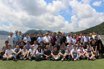](https://www.math.cuhk.edu.hk/sites/default/files/undergraduates/alumni.jpg)
* * *
### Admission Information
####
Admission Lines
* * *
#### [Enrichment Mathematics (JS4682)](#collapseEMAT)
Successful applicants are directly admitted to the Department of Mathematics. This line is for applicants who have decided to take mathematics seriously, with a strong inclination to graduate in the Enrichment Stream. See [BSc in Mathematics](/undergraduates/programmes/bsc-mathematics)
for details.
Students admitted through this line may focus more on mathematics courses in their first year of study, building a solid foundation in theoretical mathematics. Those who satisfy certain criteria will be granted the [Mathematics Scholarship](/student-centre/scholarships)
, which has no limit on the number of awardees.
#### [Broad-based Admission Scheme under the Faculty of Science (JS4601)](#collapseSCI)
Students may also apply to enter [the Science Faculty](http://www.sci.cuhk.edu.hk/en-gb/prospective-students/ug/adm/bsci)
first and then declare Mathematics as their major in their first or second year of study. They must demonstrate basic mathematical competence. There is no limit on student intake via this line.
This line is for applicants intending to explore their interests, strengths, and possible pathways early in university. Apart from concentrations in MATH, they may consider a second major or strong minor in another subject.
See [BSc in Mathematics](/undergraduates/programmes/bsc-mathematics)
for details.
#### [Mathematics and Information Engineering (JS4682 or JS4733)](#collapseMIEG)
Mathematics and Information Engineering (MIEG) is an interdisciplinary programme designed to equip gifted students with solid fundamental knowledge in mathematics as well as information and computer sciences. See [BSc in Mathematics and Information Engineering](https://www.math.cuhk.edu.hk/undergraduates/programmes/maie)
for the curriculum.
Upon completing their first year of study, students admitted through the Enrichment Mathematics (JS4682) line may switch to MIEG on a competitive basis. In this case, prospective MIEG students must declare MIEG before their second year of attendance.
Alternatively, students can apply MIEG (JS4733) directly.
On top of opportunities in MATH, MIEG students enjoy privileges exclusive to the Faculty of Engineering, including but not limited to access to engineering laboratories for coursework, work-study programmes, internships, research opportunities, competitions, scholarships and – for top students with great expectations – [the ELITE stream](http://www3.erg.cuhk.edu.hk/erg/Elite)
.
Please be reminded that MIEG students are not eligible for the Engineering and Business Administration (ERG-BBA) double degree programme offered by the Faculty of Engineering.
####
Admission Channels
* * *
#### [Local Students](#collapseL)
#### JUPAS (Joint University Programmes Admissions System)
* * *
This admission channel is for residents of Hong Kong. Local secondary school students may apply on the strength of HKDSE results. Visit [this site](http://admission.cuhk.edu.hk/jupas/requirements.html)
for detailed procedures.
Applicants must have taken a minimum of four core (C) and two elective (X, including M1/M2) subjects (4C+2X or 4C+1X+M1/M2). They must also have attained at least 3 for Chinese Language, 3 for English Language, 2 for Mathematics and 2 for Liberal Studies. In addition to satisfying the minimum University requirements, the minimum requirements for specific programmes are listed below.
| Programme | Mathematics | Mathematics
(Module 1 or 2) | Electives |
| --- | --- | --- | --- |
| Enrichment Mathematics (JS4682) | Level 4 | Level 4 | * Any one of the following subjects with Level 3:
Biology / Chemistry / Physics / Combined Science / Economics / Geography / ICT / Integrated Science / Technology and Living (Food Science & Technology) |
| Broad-based Admission Scheme under the Faculty of Science (JS4601) | Nil | Nil | * Any one of the following subjects with Level 3:
M1 or M2 / Biology / Chemistry / Physics / Combined Science / Integrated Science
* Any one subject in Category A with Level 3 |
####
Non-JUPAS
* * *
To apply on the strength of other qualifications, such as GCE-AL, IB, SAT, a higher diploma or an Associate Degree, visit [this site](http://admission.cuhk.edu.hk/non-jupas-yr-1/requirements.html)
for detailed procedures.
#### [Non-Local Students](#collapseNL)
Successful applicants are only admitted under the [Broad-based Admission Scheme under the Faculty of Science](http://www.sci.cuhk.edu.hk/en-gb/prospective-students/ug/adm/bsci)
. Prospective students need to declare Mathematics as their major in their first year of study.
####
Mainland Students
* * *
Applicants from mainland China shall apply through JEE (中華人民共和國普通高等學校聯合招生考試) on the strength of their Gaokao (內地高考). They will be admitted under the [Broad-based Admission Scheme](http://www.sci.cuhk.edu.hk/en-gb/prospective-students/ug/adm/bsci)
and declare Mathematics as their major in their first year of study. Visit [this site](http://admission.cuhk.edu.hk/sc/mainland/requirements.html)
for details.
####
International Students
* * *
Applicants from places other than Hong Kong or mainland China shall apply through this channel. Visit [this site](http://admission.cuhk.edu.hk/international/requirements.html)
for details.
---
# Prof. Bangti JIN | CUHK Mathematics
[Skip to main content](#main-content)
[](http://www.cuhk.edu.hk "The Chinese University of Hong Kong")
[](http://www.sci.cuhk.edu.hk/ "Faculty of Science")
[](/ "Home")
Search form
-----------
Search Search Search
[](https://imap.math.cuhk.edu.hk "Math Webmail")
[](/user "Login to this Math Web")
1. [Home](/)
2. [People](/people)
3. [Academic Staff](/people/academic-staff)
4. Prof. Bangti JIN
Prof. Bangti JIN
================
**Professor (Global STEM Scholar)**
_BEng, MSc (Zhejiang University);
PhD (CUHK)_
* * *
![[Teacher's name in full]](https://www.math.cuhk.edu.hk/sites/default/files/people/btjin2022.jpg)
**Address:**
Room 215, Lady Shaw Building,
The Chinese University of Hong Kong,
Shatin, N.T., Hong Kong
* * *
**Tel:**
(852) 3943-36777
* * *
**Email:**
[b.jin@cuhk.edu.hk](mailto:b.jin@cuhk.edu.hk)
* * *
**Personal Website:**
[https://www.math.cuhk.edu.hk/~btjin/](https://www.math.cuhk.edu.hk/~btjin/)
* * *
**Fields of Interest:**
inverse problems, numerical analysis, scientific computing, machine learning
* * *
**Selected Publications:**
1. Bangti Jin, Xiyao Li, Xiliang Lu. Imaging conductivity from current density magnitude using neural networks. Inverse Problems 2022; 38(7): 075003, 36 pp.
2. Bangti Jin, Yavar Kian. Recovery of the order of derivation in time-fractional differential equations in an unknown medium. SIAM Journal on Applied Mathematics 2022;82(3): 1045-1067.
3. Bangti Jin, Zehui Zhou, Jun Zou. On the saturation phenomenon of stochastic gradient descent for linear inverse problems, SIAM/ASA Journal on Uncertainty Quantification 2021; 9(4): 1553-1588.
4. Bangti Jin, Yavar Kian, Zhi Zhou. Reconstruction of a space-time dependent source in subdiffusion models via a perturbation approach. SIAM Journal on Mathematical Analysis 2021; 53(4): 4445-4473.
5. Bangti Jin, Zhi Zhou. Error analysis of finite element approximations of diffusion coefficient identification for elliptic and parabolic problems. SIAM Journal on Numerical Analysis 2021; 59(1): 119-142.
* * *
**Major Research Grants:**
* UK Engineering and Physical Science Research Council
* * *
**Professional activities:**
* editorial board, Advances in Computational Mathematics (since 2020)
* editorial board, Calcolo (since 2020)
* editorial board, Fractional Calculus & Applied Analysis (since 2021)
* editorial board, Inverse Problems (since 2019)
* editorial board, Journal of Computational Mathematics (since 2021)
* * *
#### Courses
[Current Academic Year](#teacher_current_courses_content)
----------------------------------------------------------
| Course Code | Course Title | Academic Year | Term |
| --- | --- | --- | --- |
| [MATH3230A](/course/2425/math3230a) | [Numerical Analysis](/course/math3230) | 2024/25 | 1 |
| [MATH4400C](/course/2425/math4400c) | [Project](/course/math4400) | 2024/25 | 1 |
| [MATH6221](/course/2425/math6221) | [Topics in Numerical Analysis I](/course/math6221) | 2024/25 | 1 |
| [MATH3340](/course/2425/math3340) | [Mathematics of Machine Learning](/course/math3340) | 2024/25 | 2 |
[Previous Academic Years](#teacher_previous_courses_content)
-------------------------------------------------------------
| Course Code | Course Title | Academic Year | Term |
| --- | --- | --- | --- |
| [MATH6221](/course/2324/math6221) | [Topics in Numerical Analysis I](/course/math6221) | 2023/24 | 1 |
| [MATH1010G](/course/2324/math1010g) | [University Mathematics](/course/math1010) | 2023/24 | 2 |
| [MATH3230B](/course/2324/math3230b) | [Numerical Analysis](/course/math3230) | 2023/24 | 2 |
| [MATH6221](/course/2223/math6221) | [Topics in Numerical Analysis I](/course/math6221) | 2022/23 | 1 |
| [MATH1010G](/course/2223/math1010g) | [University Mathematics](/course/math1010) | 2022/23 | 2 |
---
# Prof. Jiu Kang YU | CUHK Mathematics
[Skip to main content](#main-content)
[](http://www.cuhk.edu.hk "The Chinese University of Hong Kong")
[](http://www.sci.cuhk.edu.hk/ "Faculty of Science")
[](/ "Home")
Search form
-----------
Search Search Search
[](https://imap.math.cuhk.edu.hk "Math Webmail")
[](/user "Login to this Math Web")
1. [Home](/)
2. [People](/people)
3. [Academic Staff](/people/academic-staff)
4. Prof. Jiu Kang YU
Prof. Jiu Kang YU
=================
**Lee Hysan Professor of Mathematics**
_BSc (National Taiwan University)
PhD (Harvard University)_
* * *

**Address:**
Room 411, Academic Building No.1,
The Chinese University of Hong Kong,
Shatin, N.T., Hong Kong
* * *
**Tel:**
(852) 3943 3716
* * *
**Email:**
[jkyu@ims.cuhk.edu.hk](mailto:jkyu@ims.cuhk.edu.hk)
* * *
**Fields of Interest:**
Number theory, Representation Theory and Automorphic Forms
* * *
**Honours and Awards:**
* Fellow of the American Mathematical Society
* * *
#### Courses
[Current Academic Year](#teacher_current_courses_content)
----------------------------------------------------------
| Course Code | Course Title | Academic Year | Term |
| --- | --- | --- | --- |
| [MATH2070A](/course/2425/math2070a) | [Algebraic Structures](/course/math2070) | 2024/25 | 1 |
| [MATH4400H](/course/2425/math4400h) | [Project](/course/math4400) | 2024/25 | 1 |
| [MATH5051](/course/2425/math5051) | [Abstract Algebra I](/course/math5051) | 2024/25 | 1 |
[Previous Academic Years](#teacher_previous_courses_content)
-------------------------------------------------------------
| Course Code | Course Title | Academic Year | Term |
| --- | --- | --- | --- |
| [MATH5051](/course/2223/math5051) | [Abstract Algebra I](/course/math5051) | 2022/23 | 1 |
| [MATH2070B](/course/2122/math2070b) | [Algebraic Structures](/course/math2070) | 2021/22 | 1 |
| [MATH6031](/course/2122/math6031) | [Topics in Algebra I](/course/math6031) | 2021/22 | 1 |
| [MATH4080](/course/2122/math4080) | [Modules and Representation Theory](/course/math4080) | 2021/22 | 2 |
| [MATH3030](/course/2021/math3030) | [Abstract Algebra](/course/math3030) | 2020/21 | 1 |
| [MATH2070B](/course/2021/math2070b) | [Algebraic Structures](/course/math2070) | 2020/21 | 2 |
| [MATH3030](/course/1819/math3030) | [Abstract Algebra](/course/math3030) | 2018/19 | 1 |
| [MATH6061A](/course/1819/math6061a) | [Topics in Number Theory I](/course/math6061) | 2018/19 | 1 |
| [MATH4080](/course/1718/math4080) | [Modules and Representation Theory](/course/math4080) | 2017/18 | 2 |
| [MATH6061A](/course/1718/math6061a) | [Topics in Number Theory I](/course/math6061) | 2017/18 | 2 |
| [MATH3080](/course/1617/math3080) | [Number Theory](/course/math3080) | 2016/17 | 1 |
| [MATH4900E](/course/1617/math4900e) | [Seminar](/course/math4900) | 2016/17 | 1 |
| [MATH6061A](/course/1617/math6061a) | [Topics in Number Theory I](/course/math6061) | 2016/17 | 2 |
| [MATH3080](/course/1516/math3080) | [Number Theory](/course/math3080) | 2015/16 | 1 |
| [MATH4900B](/course/1516/math4900b) | [Seminar](/course/math4900) | 2015/16 | 1 |
| [MATH6061A](/course/1516/math6061a) | [Topics in Number Theory I](/course/math6061) | 2015/16 | 2 |
| [MATH6061A](/course/1415/math6061a) | [Topics in Number Theory I](/course/math6061) | 2014/15 | 1 |
| [MATH6062A](/course/1415/math6062a) | [Topics in Number Theory II](/course/math6062) | 2014/15 | 2 |
---
# Prof. Conan Nai Chung LEUNG | CUHK Mathematics
[Skip to main content](#main-content)
[](http://www.cuhk.edu.hk "The Chinese University of Hong Kong")
[](http://www.sci.cuhk.edu.hk/ "Faculty of Science")
[](/ "Home")
Search form
-----------
Search Search Search
[](https://imap.math.cuhk.edu.hk "Math Webmail")
[](/user "Login to this Math Web")
1. [Home](/)
2. [People](/people)
3. [Academic Staff](/people/academic-staff)
4. Prof. Conan Nai Chung LEUNG
Prof. Conan Nai Chung LEUNG
===========================
**Professor**
_MSc (University of California, San Diego)
PhD (Massachusetts Institute of Technology)_
* * *
**Address:**
Room 506, Academic Building No.1,
The Chinese University of Hong Kong,
Shatin, N.T., Hong Kong
* * *
**Tel:**
(852) 3943 8065
* * *
**Email:**
[leung@math.cuhk.edu.hk](mailto:leung@math.cuhk.edu.hk)
* * *
**Personal Website:**
[http://www.ims.cuhk.edu.hk/~leung](http://www.ims.cuhk.edu.hk/~leung)
* * *
**Fields of Interest:**
Calabi-Yau Geometry, Closed and Open Gromov-Witten Invariants, SYZ Conjecture for Mirror Symmetry, Witten-Morse Theory, Quantization, Rozansky-Witten Invariants, Hyperkähler Geometry, Geometry of Special Holonomy and ADE Bundles over Complex Surfaces
* * *
**Selected Publications:**
1. Generalization of Lawson and Simons' result to quaternion and octonion geometry, S.C. Lau and N.C. Leung
2. Moduli of Bundles over Rational Surfaces and Elliptic Curves I: Simply Laced cases, N.C. Leung and J.J. Zhang.
3. Moduli of Bundles over Rational Surfaces and Elliptic Curves II: Non-simply Laced cases, N.C. Leung and J.J. Zhang.
4. A quadratic inequality for sum of co-adjoint orbits, N.C. Leung and X.W. Wang.
5. Hard Lefschetz actions in Riemannian geometry with special holonomy, N.C. Leung and C.Z. Li.
* * *
**Major Research Grants:**
* Research Grants Council - General Research Fund
* * *
**Honours and Awards:**
* Distinguished Paper Award and Silver Award, International Consortium of Chinese Mathematicians Best Paper Award
* ICCM Best paper award
* Fellow of the American Mathematical Society
* * *
**Professional activities:**
* Editor of the New York Journal of Mathematics (NYJM) and The Asian Journal of Mathematics (AJM).
* * *
#### Courses
[Current Academic Year](#teacher_current_courses_content)
----------------------------------------------------------
| Course Code | Course Title | Academic Year | Term |
| --- | --- | --- | --- |
| [MATH6021](/course/2425/math6021) | [Topics in Geometry I](/course/math6021) | 2024/25 | 1 |
| [MATH6022](/course/2425/math6022) | [Topics in Geometry II](/course/math6022) | 2024/25 | 2 |
[Previous Academic Years](#teacher_previous_courses_content)
-------------------------------------------------------------
| Course Code | Course Title | Academic Year | Term |
| --- | --- | --- | --- |
| [MATH6021](/course/2324/math6021) | [Topics in Geometry I](/course/math6021) | 2023/24 | 1 |
| [MATH6022A](/course/2324/math6022a) | [Topics in Geometry II](/course/math6022) | 2023/24 | 2 |
| [MATH6021](/course/2223/math6021) | [Topics in Geometry I](/course/math6021) | 2022/23 | 1 |
| [MATH6022A](/course/2223/math6022a) | [Topics in Geometry II](/course/math6022) | 2022/23 | 2 |
| [MATH6021](/course/2122/math6021) | [Topics in Geometry I](/course/math6021) | 2021/22 | 1 |
| [MATH6022A](/course/2122/math6022a) | [Topics in Geometry II](/course/math6022) | 2021/22 | 2 |
| [MATH6022](/course/2021/math6022) | [Topics in Geometry II](/course/math6022) | 2020/21 | 2 |
| [MATH6021A](/course/1819/math6021a) | [Topics in Geometry I](/course/math6021) | 2018/19 | 1 |
| [MATH6022B](/course/1819/math6022b) | [Topics in Geometry II](/course/math6022) | 2018/19 | 2 |
| [MATH6021A](/course/1718/math6021a) | [Topics in Geometry I](/course/math6021) | 2017/18 | 1 |
| [MATH6022A](/course/1718/math6022a) | [Topics in Geometry II](/course/math6022) | 2017/18 | 2 |
| [MATH6021B](/course/1617/math6021b) | [Topics in Geometry I](/course/math6021) | 2016/17 | 2 |
| [MATH6021A](/course/1415/math6021a) | [Topics in Geometry I](/course/math6021) | 2014/15 | 1 |
| [MATH6022A](/course/1415/math6022a) | [Topics in Geometry II](/course/math6022) | 2014/15 | 2 |
---
# Prof. Jun ZOU | CUHK Mathematics
[Skip to main content](#main-content)
[](http://www.cuhk.edu.hk "The Chinese University of Hong Kong")
[](http://www.sci.cuhk.edu.hk/ "Faculty of Science")
[](/ "Home")
Search form
-----------
Search Search Search
[](https://imap.math.cuhk.edu.hk "Math Webmail")
[](/user "Login to this Math Web")
1. [Home](/)
2. [People](/people)
3. [Academic Staff](/people/academic-staff)
4. Prof. Jun ZOU
Prof. Jun ZOU
=============
**Chairman & Choh-Ming Li Professor of Mathematics**
_BSc (Jiangxi University)
MSc (Wuhan University)
PhD (Chinese Academy of Science)_
* * *
**ORCID:**
[0000-0002-4809-7724](https://orcid.org/0000-0002-4809-7724)
* * *
**Address:**
Room 224, Lady Shaw Building,
The Chinese University of Hong Kong,
Shatin, N.T., Hong Kong
* * *
**Tel:**
(852) 3943 7967
* * *
**Email:**
[zou@math.cuhk.edu.hk](mailto:zou@math.cuhk.edu.hk)
* * *
**Personal Website:**
[http://www.math.cuhk.edu.hk/~zou/](http://www.math.cuhk.edu.hk/~zou/)
* * *
**Fields of Interest:**
Numerical Solutions of Electromagnetic Maxwell Systems, Numerical Solutions of Interface Problems, Ill-posed Problems, Inverse Problems, Preconditioned Iterative Methods and Domain Decomposition Methods
* * *
**Selected Publications:**
1. (with Zhiming Chen and Wenlong Zhang)
Stochastic convergence of regularized solutions and their finite element approximations to inverse source problems.
SIAM J. Numer. Anal. 60 (2022), 751-780. [(PDF file)](https://www.math.cuhk.edu.hk/~zou/publication/sinum22zmchen_wlzhang.pdf)
2. (with Yat Tin Chow and Fuqun Han)
A direct sampling method for the inversion of the Radon transform.
SIAM J. Imaging Sci. 14 (2021), 1004-1038. [(PDF file)](https://www.math.cuhk.edu.hk/~zou/publication/siims21ytchow.pdf)
3. (with Yat Tin Chow and Fuqun Han) A direct sampling method for simultaneously recovering inhomogeneous inclusions of different nature.
SIAM J. Sci. Comput. 43 (2021), A2161-A2189. [(PDF file)](https://www.math.cuhk.edu.hk/~zou/publication/sisc21ytchow.pdf)
4. (with Habib Ammari and Bowen Li)
Superresolution in recovering embedded electromagnetic sources in high contrast media.
SIAM J. Imag. Sci. 13 (2020), 1467-1510. [(PDF file)](https://www.math.cuhk.edu.hk/~zou/publication/siims20ammari_bowen.pdf)
5. (wth Haijun Wu) Finite element method and its analysis for a nonlinear Helmholtz equation with high wave numbers.
SIAM J. Numer. Anal. 56 (2018), 1338-1359. [(PDF file)](https://www.math.cuhk.edu.hk/~zou/publication/sinum18hjwu.pdf)
6. (with Patrick Ciarlet, Jr. and Haijun Wu) Edge element methods for Maxwell's equations with strong convergence for Gauss' laws.
SIAM J. Numer. Anal. 52 (2014), 779-807. [(PDF file)](https://www.math.cuhk.edu.hk/~zou/publication/sinum14ciarletwu.pdf)
7. (with Hongyu Liu and Masahiro Yamamoto) Reflection principle for the Maxwell equations and its application to inverse electromagnetic scattering.
Inverse Problems 23 (2007), 2357-2366. [(PDF file)](https://www.math.cuhk.edu.hk/~zou/publication/.pdf)
8. (with R. Hiptmair and G. Widmer) Auxiliary space preconditioning in $H\_0(curl;\\Omega)$.
Numerische Mathematik 103 (2006), 435-459. [(PDF file)](https://www.math.cuhk.edu.hk/~zou/publication/numermathralf06.pdf)
9. (with Qiya Hu) A nonoverlapping domain decomposition method for Maxwell's equations in three dimensions.
SIAM J. Numer. Anal. 41 (2003), 1682-1708. [(PDF file)](https://www.math.cuhk.edu.hk/~zou/publication/sinum03b.pdf)
10. (with Eric T. Chung and Qiang Du) Convergence analysis of a finite volume method for Maxwell's equations in nonhomogeneous media.
SIAM J. Numer. Anal. 41 (2003), 37-63. [(PDF file)](https://www.math.cuhk.edu.hk/~zou/publication/sinum03a.pdf)
11. (with Qiya Hu) An iterative method with variable relaxation parameters for saddle-point problems.
SIAM J. Matrix Anal. Appl. 23 (2001), 317-338. [(PDF file)](https://www.math.cuhk.edu.hk/~zou/publication/siamtrix01hu.pdf)
12. (with Heinz W. Engl) A new approach to convergence rate analysis of Tikhonov regularization for parameter identification in heat conduction.
Inverse Problems 16 (2000), 1907-1923. [(PDF file)](https://www.math.cuhk.edu.hk/~zou/publication/inverse2000engl.pdf)
13. (with Z. Chen and Q. Du) Finite element methods with matching and nonmatching meshes for Maxwell equations with discontinuous coefficients.
SIAM J. Numer. Anal. 37 (2000), 1542-1570. [(PDF file)](https://www.math.cuhk.edu.hk/~zou/publication/sinum2000chendu.pdf)
14. (with P. Ciarlet) Fully discrete finite element approaches for time-dependent Maxwell's equations.
Numerische Mathematik 82 (1999), 193-219. [(PDF file)](https://www.math.cuhk.edu.hk/~zou/publication/numermath99ciar.pdf)
15. (with Z. Chen) An augmented Lagrangian method for identifying discontinuous parameters in elliptic systems.
SIAM J. Control Optim. 37 (1999), 892-910. [(PDF file)](https://www.math.cuhk.edu.hk/~zou/publication/siamcontrl99chen.pdf)
16. (with J. Xu) Some nonoverlapping domain decomposition methods.
SIAM Review 40 (1998), 857-914. [(PDF file)](https://www.math.cuhk.edu.hk/~zou/publication/siamreview98xu.pdf)
17. (with Z. Chen) Finite element methods and their convergence for elliptic and parabolic interface problems.
Numerische Mathematik 79 (1998), 175-202. [(PDF file)](https://www.math.cuhk.edu.hk/~zou/publication/numermath98chen.pdf)
18. (with T.F. Chan and B. Smith) Overlapping Schwarz methods on unstructublue meshes using non-matching coarse grids.
Numerische Mathematik 73 (1996), 149-167. [(PDF file)](https://www.math.cuhk.edu.hk/~zou/publication/numermath96chan.pdf)
* * *
**Major Research Grants:**
(as Principal Investigator)
* Hong Kong RGC Earmarked Grant (CUHK338/96E).
* Hong Kong RGC Earmarked Grant (CUHK4004/98E).
* Germany/Hong Kong Joint Research Scheme Grant 1998-1999 (GHK99/05).
* Hong Kong RGC Earmarked Grant (CUHK4292/00P).
* France/Hong Kong Joint Research Scheme Grant 2000-2001 (F-HKB03/00).
* Hong Kong RGC Earmarked Grant (CUHK4244/01P).
* France/Hong Kong Joint Research Scheme Grant 2001-2002 (F-HKB03/01).
* Hong Kong RGC Earmarked Grant (CUHK4048/02P).
* Hong Kong RGC Earmarked Grant (project 403403).
* Hong Kong RGC General Research Fund (project 404105).
* Hong Kong RGC General Research Fund (project 404606).
* Hong Kong RGC General Research Fund (project 404407).
* Hong Kong RGC General Research Fund (project 405110).
* Hong Kong RGC General Research Fund (project 404611).
* Hong Kong RGC General Research Fund (project 405513).
* Hong Kong RGC General Research Fund (project 14306814).
* Hong Kong RGC General Research Fund (project 14322516).
* Hong Kong RGC/NSFC Joint Scheme (project N-CUHK437/16).
* Hong Kong RGC General Research Fund (project 14304517).
* Hong Kong RGC General Research Fund (project 14306718).
* Hong Kong RGC General Research Fund (project 14306719).
* * *
**Honours and Awards:**
* Fellow, The American Mathematical Society (AMS), 2022
* Fellow, The Society for Industrial and Applied Mathematics (SIAM), 2019.
* * *
**Professional activities:**
##### **Associate editors of the journals**
* January 2013 -- present :
[ESAIM: Mathematical Modelling and Numerical Analysis](https://www.esaim-m2an.org/about-the-journal/editorial-board)
(M2AN).
French Society for Applied and Industrial Mathematics & Cambridge University Press.
* January 2018 -- present :
[SIAM Journal on Numerical Analysis](https://www.siam.org/journals/sinum.php)
(SINUM).
Society for Industrial and Applied Mathematics, USA.
* November 2012 -- present :
[Inverse Problems and Imaging](https://www.aimsciences.org/journal/1930-8337/editorialboard)
(IPI).
American Institute of Mathematical Sciences, USA.
* January 2018 -- present :
[SIAM Journal on Scientific Computing](https://www.siam.org/journals/sisc.php)
(SISC).
Society for Industrial and Applied Mathematics, USA.
* January 2017 -- present :
[Computational Methods in Applied Mathematics](https://www.degruyter.com/view/j/cmam)
(CMAM).
De Gruyter, Germany.
* May 2017 -- present :
[Numerical Algorithms](https://link.springer.com/journal/11075)
.
Springer, Germany.
* June 2011 -- present :
[Applicable Analysis](http://www.tandfonline.com/toc/gapa20/current/)
.
Taylor & Francis, UK.
* March 2006 -- present :
[Journal of Numerical Mathematics](https://www.degruyter.com/view/j/jnma)
.
Brill Academic Publishers, The Netherlands.
* January 2005 -- present :
[Journal of Inverse and Ill-posed Problems](https://www.degruyter.com/view/j/jiip)
(JIIP).
VSP, The Netherlands.
* January 2019 -- present :
[Results in Applied Mathematics](https://www.journals.elsevier.com/results-in-applied-mathematics)
.
Elsevier, The Netherlands.
* January 2004 -- June 2020 :
[International Journal of Numerical Analysis & Modeling](http://www.math.ualberta.ca/ijnam/)
.
IJNAM Publisher, Canada.
* * *
#### Courses
[Current Academic Year](#teacher_current_courses_content)
----------------------------------------------------------
| Course Code | Course Title | Academic Year | Term |
| --- | --- | --- | --- |
| [MATH3230B](/course/2425/math3230b) | [Numerical Analysis](/course/math3230) | 2024/25 | 2 |
[Previous Academic Years](#teacher_previous_courses_content)
-------------------------------------------------------------
| Course Code | Course Title | Academic Year | Term |
| --- | --- | --- | --- |
| [MATH3230A](/course/2324/math3230a) | [Numerical Analysis](/course/math3230) | 2023/24 | 1 |
| [MATH3230](/course/2223/math3230) | [Numerical Analysis](/course/math3230) | 2022/23 | 1 |
| [MATH3230](/course/2122/math3230) | [Numerical Analysis](/course/math3230) | 2021/22 | 1 |
| [MATH3230A](/course/2021/math3230a) | [Numerical Analysis](/course/math3230) | 2020/21 | 1 |
| [MATH3230A](/course/1920/math3230a) | [Numerical Analysis](/course/math3230) | 2019/20 | 1 |
| [MATH3230A](/course/1718/math3230a) | [Numerical Analysis](/course/math3230) | 2017/18 | 1 |
| [MATH3240](/course/1718/math3240) | [Numerical Methods for Differential Equations](/course/math3240) | 2017/18 | 2 |
| [MATH4900G](/course/1617/math4900g) | [Seminar](/course/math4900) | 2016/17 | 1 |
| [MATH3230B](/course/1617/math3230b) | [Numerical Analysis](/course/math3230) | 2016/17 | 2 |
| [MATH3240](/course/1617/math3240) | [Numerical Methods for Differential Equations](/course/math3240) | 2016/17 | 2 |
| [MATH3230A](/course/1516/math3230a) | [Numerical Analysis](/course/math3230) | 2015/16 | 1 |
| [MATH3230B](/course/1516/math3230b) | [Numerical Analysis](/course/math3230) | 2015/16 | 2 |
| [MATH3240](/course/1516/math3240) | [Numerical Methods for Differential Equations](/course/math3240) | 2015/16 | 2 |
| [MATH3230A](/course/1415/math3230a) | [Numerical Analysis](/course/math3230) | 2014/15 | 1 |
| [MATH3413B](/course/1415/math3413b) | [Seminar I](/course/math3413) | 2014/15 | 1 |
| [MATH3413C](/course/1415/math3413c) | [Seminar I](/course/math3413) | 2014/15 | 1 |
| [MATH3230B](/course/1415/math3230b) | [Numerical Analysis](/course/math3230) | 2014/15 | 2 |
| [MATH3423B](/course/1415/math3423b) | [Seminar II](/course/math3423) | 2014/15 | 2 |
---
# Bangti Jin's Homepage
**Welcome to the Homepage of Bangti Jin**
### I am a Professor of Mathematics (Global STEM Scholar), at [Department of Mathematics](https://www.math.cuhk.edu.hk/)
, [The Chinese University of Hong Kong](http://www.cuhk.edu.hk/)
. My research areas is applied and computational mathematics, and I am particularly interested in computational inverse problems, numerical analysis, machine learning, and scientific computing.
### I am on the editorial boards of the following journals: [Advances in Computational Mathematics](https://www.springer.com/journal/10444)
(Springer), [Calcolo](https://www.springer.com/journal/10092)
(Springer), [Fractional Calculus and Applied Analysis](https://www.springer.com/journal/13540)
(Springer), [Inverse Problems](https://iopscience.iop.org/journal/0266-5611)
(Institute of Physics) and [Journal of Computational Mathematics](https://www.global-sci.org/jcm/)
(Global Science).
**Address:** Room 215, Lady Shaw Building, Department of Mathematics, The Chinese University of Hong Kong, Shatin, New Territories, Hong Kong
**Tel**: (852) 3943 6777
**Email**: b.jin AT cuhk.edu.hk
**[Publications](publications.htm)
**
**[Research group](group.htm)
**
**[Inverse Problems Seminar](ipseminar.htm)
**
**[Teaching](teaching.htm)
**
**[Openings (new)](opening.htm)
**
---
# Prof. Zhouping XIN | CUHK Mathematics
[Skip to main content](#main-content)
[](http://www.cuhk.edu.hk "The Chinese University of Hong Kong")
[](http://www.sci.cuhk.edu.hk/ "Faculty of Science")
[](/ "Home")
Search form
-----------
Search Search Search
[](https://imap.math.cuhk.edu.hk "Math Webmail")
[](/user "Login to this Math Web")
1. [Home](/)
2. [People](/people)
3. [Academic Staff](/people/academic-staff)
4. Prof. Zhouping XIN
Prof. Zhouping XIN
==================
**William M.W. Mong Professor of Mathematics**
_BS (Northwestern University)
MS (Academia Sinica)
PhD (University of Michigan)_
* * *

**Address:**
Room 701, Academic Building No.1,
The Chinese University of Hong Kong,
Shatin, N.T., Hong Kong
* * *
**Tel:**
(852) 3943 4100
* * *
**Email:**
[zpxin@ims.cuhk.edu.hk](mailto:zpxin@ims.cuhk.edu.hk)
* * *
**Personal Website:**
[http://www.ims.cuhk.edu.hk/people/staff/zpxin/](http://www.ims.cuhk.edu.hk/people/staff/zpxin/)
* * *
**Fields of Interest:**
Partial Differential Equations, Fluid Dynamics and Nonlinear Waves
* * *
**Selected Publications:**
1. Subsonic flows past a profile with a vortex line at the trailing edge, (with Jun Chen, Aibin Zang), SIAM J. Math. Anal., 54, No. 1, 912-939 (2022).
2. On Some Smooth Symmetric Transonic Flows with Nonzero Angular Velocity and Vorticity, (with S. K. Weng, H. W. Yuan), submitted to M3AS: Math. Models Methods Appl. Sci., 31, no. 13, 2773-2817 (2021).
3. Global well-posedness of regular solutions to the three-dimensional isentropic compressible Navier-Stokes equations with degenerate viscosities and vacuum, (with S. G. Zhu), Advances in Mathematics, 393, [https://doi.org/10.1016/j.aim.2021.108072](https://doi.org/10.1016/j.aim.2021.108072)
(2021).
4. Global Well-Posedness of Free Interface Problems for the Incompressible Inviscid Resistive MHD, (with Yanjin Wang), Commun. Math. Phys, [http://doi.org/10.1007/s00220-021-04235-3](http://doi.org/10.1007/s00220-021-04235-3)
(2021).
5. Global Well-Posedness of the Inviscid Heat-Conductive Resistive Compressible MHD in a Strip Domain, (with Yanjin Wang), Commun. Math. Res., Vol. 38, No. 1, pp. 1-27 (2021).
* * *
**Major Research Grants:**
* PI, RGC General Research Fund 2021/22, Well-Posedness of The Contact Discontinuities for the Ideal MHD, 14301421, 01/01/2022 – 31/12/2024
* PI, RGC General Research Fund 2019/20, Regularity estimates of Hessian and Curvature equations, 14300819, 01/11/2019 – 31/10/2022
* PI, RGC General Research Fund 2019/20, Vacuum Dynamics for the Full Compressible Navier-Stokes Equations, 14302819, 01/01/2020 - 31/12/2022
* PI, RGC General Research Fund 2017/18, On Some Problems for Steady Compressible Euler Systems, 14300917, 01/01/2018 - 31/12/2021
* PI, RGC General Research Fund 2017/18, Weak and Strong Solutions to the Primitive Equations with Full or Horizontal Viscosity but No Diffusivity, 14302917, 01/09/2017 - 28/02/2021
* * *
**Honours and Awards:**
* Top 1000 Scientists in Mathematicians, 2022
* Qin Yuan Xun Mathematical Award, 08/2019
* Distinguished Paper Award (Silver), International Consortium of Chinese Mathematicians, 2017
* Changjiang Scholar, Ministry of Education of China, 2006-2008
* Morningside Gold Medalist in Mathematics, International Congress of Chinese Mathematicians, 12/2004
* * *
**Professional activities:**
* Member, and Member of Academic Committee, International Consortium of Chinese Mathematicians (ICCM) since 08/2016
* Council Member at Large, Hong Kong Mathematical Society, since 05/2016
* President, Hong Kong Mathematical Society, 05/2012 - 04/2016
* Vice President, Hong Kong Mathematical Society, 05/2004 - 04/2012
* Member, Hong Kong Mathematical Society, since 09/1998
* * *
#### Courses
[Current Academic Year](#teacher_current_courses_content)
----------------------------------------------------------
| Course Code | Course Title | Academic Year | Term |
| --- | --- | --- | --- |
| [MATH6041](/course/2425/math6041) | [Topics in Differential Equations I](/course/math6041) | 2024/25 | 1 |
[Previous Academic Years](#teacher_previous_courses_content)
-------------------------------------------------------------
| Course Code | Course Title | Academic Year | Term |
| --- | --- | --- | --- |
| [MATH6041A](/course/2324/math6041a) | [Topics in Differential Equations I](/course/math6041) | 2023/24 | 1 |
| [MATH6041](/course/2223/math6041) | [Topics in Differential Equations I](/course/math6041) | 2022/23 | 1 |
| [MATH6041](/course/2122/math6041) | [Topics in Differential Equations I](/course/math6041) | 2021/22 | 1 |
| [MATH6041](/course/2021/math6041) | [Topics in Differential Equations I](/course/math6041) | 2020/21 | 1 |
| [MATH6041A](/course/1920/math6041a) | [Topics in Differential Equations I](/course/math6041) | 2019/20 | 1 |
| [MATH6041A](/course/1819/math6041a) | [Topics in Differential Equations I](/course/math6041) | 2018/19 | 1 |
| [MATH6041A](/course/1718/math6041a) | [Topics in Differential Equations I](/course/math6041) | 2017/18 | 1 |
| [MATH4220](/course/1718/math4220) | [Partial Differential Equations](/course/math4220) | 2017/18 | 2 |
| [MATH4220](/course/1617/math4220) | [Partial Differential Equations](/course/math4220) | 2016/17 | 2 |
| [MATH4220](/course/1516/math4220) | [Partial Differential Equations](/course/math4220) | 2015/16 | 2 |
| [MATH3270A](/course/1415/math3270a) | [Ordinary Differential Equations](/course/math3270) | 2014/15 | 1 |
---
# CUHK Innovation Day 2024 | CUHK Mathematics
[Skip to main content](#main-content)
[](http://www.cuhk.edu.hk "The Chinese University of Hong Kong")
[](http://www.sci.cuhk.edu.hk/ "Faculty of Science")
[](/ "Home")
Search form
-----------
Search Search Search
[](https://imap.math.cuhk.edu.hk "Math Webmail")
[](/user "Login to this Math Web")
1. [Home](/)
2. [News](/news)
3. CUHK Innovation Day 2024
CUHK Innovation Day 2024
========================
Date Posted:
6 September, 2024
[](https://innovationday2024.cuhk.edu.hk/registration)
---
# Prof. Renjun DUAN | CUHK Mathematics
[Skip to main content](#main-content)
[](http://www.cuhk.edu.hk "The Chinese University of Hong Kong")
[](http://www.sci.cuhk.edu.hk/ "Faculty of Science")
[](/ "Home")
Search form
-----------
Search Search Search
[](https://imap.math.cuhk.edu.hk "Math Webmail")
[](/user "Login to this Math Web")
1. [Home](/)
2. [People](/people)
3. [Academic Staff](/people/academic-staff)
4. Prof. Renjun DUAN
Prof. Renjun DUAN
=================
**Professor**
_BSc, MS (Central China Normal University)
PhD (City University of Hong Kong)_
* * *

**ORCID:**
[0000-0001-8821-8829](https://orcid.org/0000-0001-8821-8829)
* * *
**Address:**
Room 206, Lady Shaw Building,
The Chinese University of Hong Kong,
Shatin, N.T., Hong Kong
* * *
**Tel:**
(852) 3943 7977
* * *
**Email:**
[rjduan@math.cuhk.edu.hk](mailto:rjduan@math.cuhk.edu.hk)
* * *
**Personal Website:**
[http://www.math.cuhk.edu.hk/~rjduan/](http://www.math.cuhk.edu.hk/~rjduan/)
* * *
**Fields of Interest:**
PDEs related to kinetic and fluid dynamic equations
* * *
**Selected Publications:**
1. Renjun Duan and Shuangqian Liu, _Compressible Navier-Stokes approximation for the Boltzmann equation in bounded domains_. Transactions of the American Mathematical Society, 374 (2021), no. 11, 7867-7924.
2. Renjun Duan, Dongcheng Yang, and Hongjun Yu, _Small Knudsen rate of convergence to rarefaction wave for the Landau equation_. Archive for Rational Mechanics and Analysis, 240 (2021), no. 3,1535-1592.
3. Renjun Duan, Shuangqian Liu, Shota Sakamoto, and Robert M. Strain, _Global mild solutions of the Landau and non-cutoff Boltzmann equations_. Communications on Pure and Applied Mathematics, 74 (2021), no. 5, 932-1020.
4. Yoshihiro Ueda, Renjun Duan and Shuichi Kawashima, _Decay structure for symmetric hyperbolic systems with non-symmetric relaxation and its application_. Archive for Rational Mechanics and Analysis, 205 (2012), no. 1, 239-266.
5. Renjun Duan and Robert M. Strain, _Optimal large-time behavior of the Vlasov-Maxwell-Boltzmann system in the whole space_. Communications on Pure and Applied Mathematics, 64 (2011), no. 11, 1497-1546.
6. Renjun Duan, Alexander Lorz and Peter Markowich, _Global solutions to the coupled chemotaxis-fluid equations_. Communications in Partial Differential Equations, 35 (2010), no. 9, 1635-1673.
7. Renjun Duan, Massimo Fornasier and Giuseppe Toscani, _A kinetic flocking model with diffusions_. Communications in Mathematical Physics, 300 (2010), no. 1, 95-145.
* * *
**Major Research Grants:**
* National Natural Science Foundation of China and Hong Kong Research Grant Council - Joint Research Scheme
* Research Grants Council - General Research Fund
* * *
**Honours and Awards:**
* Hong Kong Mathematical Society Young Scholar Award
* * *
**Professional activities:**
* Editorial board - Nonlinear Analysis: Real World Applications (Board member, 08/2018-present)
* Editorial board - Discrete & Continuous Dynamical Systems – B (Board member, 01/2020-present)
* Editorial board - Kinetic and Related Models (Associate editor, 01/2022-present)
* Editorial board - Communications in Mathematical Analysis and Applications (Managing editor, 01/2022-present)
* * *
#### Courses
[Current Academic Year](#teacher_current_courses_content)
----------------------------------------------------------
| Course Code | Course Title | Academic Year | Term |
| --- | --- | --- | --- |
| [MATH2040A](/course/2425/math2040a) | [Linear Algebra II](/course/math2040) | 2024/25 | 1 |
| [MATH2060C](/course/2425/math2060c) | [Mathematical Analysis II](/course/math2060) | 2024/25 | 2 |
| [MATH4240](/course/2425/math4240) | [Stochastic Processes](/course/math4240) | 2024/25 | 2 |
[Previous Academic Years](#teacher_previous_courses_content)
-------------------------------------------------------------
| Course Code | Course Title | Academic Year | Term |
| --- | --- | --- | --- |
| [MATH2060A](/course/2324/math2060a) | [Mathematical Analysis II](/course/math2060) | 2023/24 | 2 |
| [MATH4240](/course/2324/math4240) | [Stochastic Processes](/course/math4240) | 2023/24 | 2 |
| [MATH2040A](/course/2223/math2040a) | [Linear Algebra II](/course/math2040) | 2022/23 | 1 |
| [MATH4240](/course/2223/math4240) | [Stochastic Processes](/course/math4240) | 2022/23 | 2 |
| [MATH6042](/course/2223/math6042) | [Topics in Differential Equations II](/course/math6042) | 2022/23 | 2 |
| [MATH2040A](/course/2122/math2040a) | [Linear Algebra II](/course/math2040) | 2021/22 | 1 |
| [MATH4240](/course/2122/math4240) | [Stochastic Processes](/course/math4240) | 2021/22 | 2 |
| [MATH2040A](/course/2021/math2040a) | [Linear Algebra II](/course/math2040) | 2020/21 | 1 |
| [MATH4240](/course/2021/math4240) | [Stochastic Processes](/course/math4240) | 2020/21 | 2 |
| [MATH6042](/course/2021/math6042) | [Topics in Differential Equations II](/course/math6042) | 2020/21 | 2 |
| [MATH2040A](/course/1920/math2040a) | [Linear Algebra II](/course/math2040) | 2019/20 | 1 |
| [MATH4240](/course/1920/math4240) | [Stochastic Processes](/course/math4240) | 2019/20 | 2 |
| [MATH6042A](/course/1920/math6042a) | [Topics in Differential Equations II](/course/math6042) | 2019/20 | 2 |
| [MATH2040A](/course/1819/math2040a) | [Linear Algebra II](/course/math2040) | 2018/19 | 1 |
| [MATH4240](/course/1819/math4240) | [Stochastic Processes](/course/math4240) | 2018/19 | 2 |
| [MATH6042](/course/1819/math6042) | [Topics in Differential Equations II](/course/math6042) | 2018/19 | 2 |
| [MATH4240](/course/1718/math4240) | [Stochastic Processes](/course/math4240) | 2017/18 | 2 |
| [MATH6041B](/course/1718/math6041b) | [Topics in Differential Equations I](/course/math6041) | 2017/18 | 2 |
| [MATH2010A](/course/1617/math2010a) | [Advanced Calculus I](/course/math2010) | 2016/17 | 1 |
| [MATH4240](/course/1617/math4240) | [Stochastic Processes](/course/math4240) | 2016/17 | 2 |
| [MATH5022](/course/1617/math5022) | [Theory of Partial Differential Equations II](/course/math5022) | 2016/17 | 2 |
| [MATH4240](/course/1516/math4240) | [Stochastic Processes](/course/math4240) | 2015/16 | 2 |
| [MATH5022](/course/1516/math5022) | [Theory of Partial Differential Equations II](/course/math5022) | 2015/16 | 2 |
| [MATH2010A](/course/1415/math2010a) | [Advanced Calculus I](/course/math2010) | 2014/15 | 1 |
| [MATH2020B](/course/1415/math2020b) | [Advanced Calculus II](/course/math2020) | 2014/15 | 2 |
| [MATH4220](/course/1415/math4220) | [Partial Differential Equations](/course/math4220) | 2014/15 | 2 |
---
# BSc in Mathematics | CUHK Mathematics
[Skip to main content](#main-content)
[](http://www.cuhk.edu.hk "The Chinese University of Hong Kong")
[](http://www.sci.cuhk.edu.hk/ "Faculty of Science")
[](/ "Home")
Search form
-----------
Search Search Search
[](https://imap.math.cuhk.edu.hk "Math Webmail")
[](/user "Login to this Math Web")
1. [Home](/)
2. [Undergraduates](/undergraduates)
3. [Programmes](/undergraduates/programmes)
4. BSc in Mathematics
BSc in Mathematics
==================
**The following details are for reference only. Students are advised to visit** [**Undergraduate** **Student Handbook**](https://rgsntl.rgs.cuhk.edu.hk/aqs_prd_applx/public/handbook/default.aspx)
**or** **[CUSIS](http://rgsntl.rgs.cuhk.edu.hk/aqs_prd_applx/Public/tt_dsp_acad_prog.aspx)** **for the latest curriculum, which depends on the year of admission.**
###
Programme Features
* * *
Students take the same mandatory fundamental courses in their first two years of study, and can choose from a wide range of courses according to their interests, abilities, and career aspirations.
We have designated five graduation pathways, or streams, as goals for different students. For students who focus on reaching their goals, a fulfilling and rewarding undergraduate journey awaits.
Prospective students are welcome to explore the [Student Centre](/student-centre)
, where they can find [academic advice](/student-centre/academic-advice)
, [scholarship information](/student-centre/scholarships)
and details about the [COSINE program](/student-centre/cosine-program)
. Current students may also approach our [academic advisors](/people/administration)
for enquiries.
Note that MATH streams are not mutually exclusive. There is no limit to the number of streams in which a MATH student can graduate.
###
Study Scheme
* * *
Students are required to complete the following courses:
* 9 units of the Science Faculty Package in Physics, Chemistry, Life Sciences, Statistics and Mathematics;
* 35 units of fundamental Mathematics courses;
* 27 units of elective courses
For details of the streams, please visit [this page](https://www.math.cuhk.edu.hk/undergraduates/streams)
.
* * *
**Science, Technology And Research Stream (STARS) \[applicable to 2017-18 cohort\]**
In addition to fulfilling the above Major Programme Requirement, students meeting the criteria as specified by the Faculty of Science can take Science, Technology And Research Stream (STARS) offered by the Faculty.
Students are required to complete a minimum of 12 units of courses as follows:
1\. Required Courses:
* 3 units of the Science Faculty Package Course (Choose from the two remaining groups of the Faculty Package that have not been used to fulfill the Faculty Package Requirement) ;
* 6 units of Research Courses;
* 3 units of Seminar Courses
2\. Experiential Learning:
* At least 4 consecutive weeks of outside Hong Kong exposure
---
# Mathematical Modelling @ CUHK Mathematics
Mathematical Modelling @ CUHK Mathematics
=========================================
#### What is Mathematical Modelling? 甚麼是數學建模?

* * *
[The Department of Mathematics](https://www.math.cuhk.edu.hk/)
at [The Chinese University of Hong Kong](https://www.cuhk.edu.hk/)
is dedicated to making a positive impact on promoting mathematical modelling for teachers and students in secondary schools in Hong Kong.
[香港中文大學](https://www.cuhk.edu.hk/)
[數學系](https://www.math.cuhk.edu.hk/)
致力向香港中學師生推廣數學建模。
Since 2024, we have organized a series of mathematical modelling [workshops](workshop.html)
for teachers and students and [mathematical modelling competitions](competition.html)
.
自2024年起,我們舉辦了一系列的數學建模教師與學生[工作坊](workshop.html)
及[數學建模比賽](competition.html)
。
We are also providing various mathematical modelling [teaching and learning resources](learning.html)
and [interactive IT tools](tool.html)
for teachers and students to experience mathematical modelling.
我們亦提供不同的數學建模[教學資源](learning.html)
和[互動式 IT 工具](tool.html)
,供教師和學生體驗數學建模。
Last updated: 09/02/2025
[Back to top 回到頂部](index.html#)
---
# Prof. Kwok Wai CHAN | CUHK Mathematics
[Skip to main content](#main-content)
[](http://www.cuhk.edu.hk "The Chinese University of Hong Kong")
[](http://www.sci.cuhk.edu.hk/ "Faculty of Science")
[](/ "Home")
Search form
-----------
Search Search Search
[](https://imap.math.cuhk.edu.hk "Math Webmail")
[](/user "Login to this Math Web")
1. [Home](/)
2. [People](/people)
3. [Academic Staff](/people/academic-staff)
4. Prof. Kwok Wai CHAN
Prof. Kwok Wai CHAN
===================
**Professor**
_BSc, MPhil, PhD (The Chinese University of Hong Kong)_
* * *
**ORCID:**
[0000-0003-1113-6758](https://orcid.org/0000-0003-1113-6758)
* * *
**Address:**
Room 212, Lady Shaw Building,
The Chinese University of Hong Kong,
Shatin, N.T., Hong Kong
* * *
**Tel:**
(852) 3943 7976
* * *
**Email:**
[kwchan@math.cuhk.edu.hk](mailto:kwchan@math.cuhk.edu.hk)
* * *
**Personal Website:**
[http://www.math.cuhk.edu.hk/~kwchan/](http://www.math.cuhk.edu.hk/~kwchan/)
* * *
**Fields of Interest:**
Complex Geometry, Mirror Symmetry, Quantization
* * *
**Selected Publications:**
1. K. Chan, Z. N. Ma and Y.-H. Suen, Tropical Lagrangian multi-sections and smoothing of locally free sheaves over degenerate Calabi-Yau surfaces, **Advances in Mathematics** 401 (2022), 108280, 37 pp.
2. K. Chan, N. C. Leung and Z. N. Ma, _Scattering diagrams from asymptotic analysis on Maurer-Cartan equations_, **Journal of the European Mathematical Society (JEMS)** 24 (2022), no. 3, 773-849.
3. K. Chan, N. C. Leung and Q. Li, _Bargmann-Fock sheaves on Kähler manifolds_, **Communications in Mathematical Physics** 388 (2021), no. 3, 1297-1322.
4. K. Chan, S.-C. Lau, N. C. Leung and H.-H. Tseng, _Open Gromov-Witten invariants, mirror maps, and Seidel representations for toric manifolds,_ **Duke Mathematical Journal** 166 (2017), no. 8, 1405-1462.
5. K. Chan, C.-H. Cho, S.-C. Lau and H.-H. Tseng, _Gross fibrations, SYZ mirror symmetry, and open Gromov-Witten invariants for toric Calabi-Yau orbifolds_, **Journal of Differential Geometry** 103 (2016), no. 2, 207-288.
6. K. Chan, D. Pomerleano and K. Ueda, _Lagrangian torus fibrations and homological mirror symmetry for the conifold,_ **Communications in Mathematical Physics** 341 (2016), no. 1, 135-178.
7. K. Chan, C.-H. Cho, S.-C. Lau and H.-H. Tseng, _Lagrangian Floer superpotentials and crepant resolutions for toric orbifolds,_ **Communications in Mathematical Physics** 328 (2014), no. 1, 83-130.
8. K. Chan, S.-C. Lau and H.-H. Tseng, _Enumerative meaning of mirror maps for toric Calabi-Yau manifolds_, **Advances in Mathematics** 244 (2013), 605-625.
9. K. Chan, S.-C. Lau and N. C. Leung, _SYZ mirror symmetry for toric Calabi-Yau manifolds_, **Journal of Differential Geometry** 90 (2012), no. 2, 177-250.
10. K. Chan and N. C. Leung, _Mirror symmetry for toric Fano manifolds via SYZ transformations_, **Advances in Mathematics** 223 (2010), no. 3, 797-839.
* * *
**Major Research Grants:**
* Research Grants Council - General Research Fund
* * *
**Honours and Awards:**
* Hong Kong Mathematical Society Young Scholar Award
* ICCM Best paper award
* Vice-Chancellor's Exemplary Teaching Award
* Distinguished Paper Award and Silver Award, International Consortium of Chinese Mathematicians Best Paper Award
* Faculty Exemplary Teaching Award
* * *
**Professional activities:**
* Editor, The Asian Journal of Mathematics (AJM), 01/2022 - present
* * *
#### Courses
[Current Academic Year](#teacher_current_courses_content)
----------------------------------------------------------
| Course Code | Course Title | Academic Year | Term |
| --- | --- | --- | --- |
| [MATH3030](/course/2425/math3030) | [Abstract Algebra](/course/math3030) | 2024/25 | 1 |
[Previous Academic Years](#teacher_previous_courses_content)
-------------------------------------------------------------
| Course Code | Course Title | Academic Year | Term |
| --- | --- | --- | --- |
| [MATH3030](/course/2324/math3030) | [Abstract Algebra](/course/math3030) | 2023/24 | 1 |
| [MMAT5120](/course/2324/mmat5120) | [Topics in Geometry](/course/mmat5120) | 2023/24 | 1 |
| [MATH2078](/course/2324/math2078) | [Honours Algebraic Structures](/course/math2078) | 2023/24 | 2 |
| [MATH3030](/course/2223/math3030) | [Abstract Algebra](/course/math3030) | 2022/23 | 1 |
| [MATH2078](/course/2223/math2078) | [Honours Algebraic Structures](/course/math2078) | 2022/23 | 2 |
| [MATH3030](/course/2122/math3030) | [Abstract Algebra](/course/math3030) | 2021/22 | 1 |
| [MATH4900B](/course/2122/math4900b) | [Seminar](/course/math4900) | 2021/22 | 1 |
| [MATH2078](/course/2122/math2078) | [Honours Algebraic Structures](/course/math2078) | 2021/22 | 2 |
| [MMAT5120](/course/2122/mmat5120) | [Topics in Geometry](/course/mmat5120) | 2021/22 | 2 |
| [MATH3040](/course/2021/math3040) | [Fields and Galois Theory](/course/math3040) | 2020/21 | 2 |
| [MATH6031](/course/2021/math6031) | [Topics in Algebra I](/course/math6031) | 2020/21 | 2 |
| [MATH2070A](/course/1920/math2070a) | [Algebraic Structures](/course/math2070) | 2019/20 | 1 |
| [MATH4900C](/course/1920/math4900c) | [Seminar](/course/math4900) | 2019/20 | 1 |
| [MATH6031A](/course/1920/math6031a) | [Topics in Algebra I](/course/math6031) | 2019/20 | 2 |
| [MMAT5220](/course/1920/mmat5220) | [Complex Analysis and Its Applications](/course/mmat5220) | 2019/20 | 2 |
| [MATH2040B](/course/1819/math2040b) | [Linear Algebra II](/course/math2040) | 2018/19 | 1 |
| [MATH2070A](/course/1819/math2070a) | [Algebraic Structures](/course/math2070) | 2018/19 | 1 |
| [MATH3040](/course/1819/math3040) | [Fields and Galois Theory](/course/math3040) | 2018/19 | 2 |
| [MATH2070A](/course/1718/math2070a) | [Algebraic Structures](/course/math2070) | 2017/18 | 1 |
| [MATH3030](/course/1718/math3030) | [Abstract Algebra](/course/math3030) | 2017/18 | 1 |
| [MATH1030E](/course/1718/math1030e) | [Linear Algebra I](/course/math1030) | 2017/18 | 2 |
| [MATH1030C](/course/1617/math1030c) | [Linear Algebra I](/course/math1030) | 2016/17 | 1 |
| [MATH3030](/course/1617/math3030) | [Abstract Algebra](/course/math3030) | 2016/17 | 1 |
| [MATH3040](/course/1617/math3040) | [Fields and Galois Theory](/course/math3040) | 2016/17 | 2 |
| [MATH1030C](/course/1516/math1030c) | [Linear Algebra I](/course/math1030) | 2015/16 | 1 |
| [MATH3030](/course/1516/math3030) | [Abstract Algebra](/course/math3030) | 2015/16 | 1 |
| [MATH3030](/course/1415/math3030) | [Abstract Algebra](/course/math3030) | 2014/15 | 1 |
| [MATH6031A](/course/1415/math6031a) | [Topics in Algebra I](/course/math6031) | 2014/15 | 1 |
| [MATH3040](/course/1415/math3040) | [Fields and Galois Theory](/course/math3040) | 2014/15 | 2 |
---
# Unknown
**Opening****:** I am always looking for highly motivated and passionate PhD students and postdocs to join my group. If you are interested in working with me, please feel free to email me to discuss the possibilities.
**PhD Students:**
1. Mr. Tianhao Hu (CUHK, 2023 - now)
2. Mr. Jason Choy (CUHK, 2023 - now)
3. Ms. Yuxin Fan (CUHK, 2023 - now)
4. Mr. Luowei Yin (The Chinese University of Hong Kong, 2022 - now)
5. Ms. Xiyao Li (University College London, 2020 - now)
6. Mr. Riccardo Barbano (University College London, 2019 - 2023)
**Postdocs**
1. Dr. Fengru Wang (PhD university: Wuhan University, 2023 - now)
2. Dr. Qimeng Quan (PhD university: Wuhan University, 2023 - now)
3. Dr. Ramesh Chandra Sau (PhD university: Indian Institute of Science, Bangalore, 2022 - now)
**Alumni (PhD students)**
1. Chen Zhang (University College London, PhD student, 2016 - 2020)
2. Zhi Zhou (Texas A&M University, 2011 - 2015, PhD student, co-supervisor)
3. Matthias Gehre (University of Bremen, 2010 - 2013, PhD student, co-supervisor)
**Alumni (postdocs)**
1. Dr. Zeljko Kereta (PhD university: ETH Zurich, 2019 - 2022)
2. Dr. Youzi He (PhD university: Hong Kong Baptist University, 2022 - 2023)
---
# Further Graduate Studies | CUHK Mathematics
[Skip to main content](#main-content)
[](http://www.cuhk.edu.hk "The Chinese University of Hong Kong")
[](http://www.sci.cuhk.edu.hk/ "Faculty of Science")
[](/ "Home")
Search form
-----------
Search Search Search
[](https://imap.math.cuhk.edu.hk "Math Webmail")
[](/user "Login to this Math Web")
1. [Home](/)
2. [People](/people)
3. Further Graduate Studies
Further Graduate Studies
========================
Every year, many of our graduates pursue further graduate studies in local institutions and abroad, preparing themselves for careers in both academia and industry. Despite keen global competition for entering top universities, our graduates have performed outstandingly in their graduate school applications.
Our students are well-trained through our undergraduate program to learn efficiently and to transcend their academic abilities and to do frontier research in mathematics and other fields. By raising student research standards, we also contribute to the international academic community by preparing Hong Kong students for further education, many of them have become active mathematicians internationally.
If you are a CUHK Mathematics graduate who has studied for a second degree, and your name is not listed below, please fill in [this form](https://www.math.cuhk.edu.hk/people/alumni/advanced-study/overseas-study-form)
and we will get back to you shortly. Thank you very much.
#### [2021 - Present](#collapse2021)
#### **2024
Overseas**
* * *
* **Ric Lim COO**
National University of Singapore \[Mathematics\]
* **Yiqi HUANG**
Massachusetts Institute of Technology \[Geometric Analysis and Partial Differential Equations\]
* **Yu Chung HUNG**
Texas A&M University \[Mathematics\]
* **Matthew Jamie LIU**
University of Alberta \[Mathematics\]
* **Tianyu LU**
Northeastern University \[Applied Mathematics\]
* **Chun Hei Michael SHIU**
The University of British Columbia \[Electrical and Computer Engineering\]
* **Sin Hang Jason YEUNG**
University of Toronto \[Mathematics\]
* **Wing Lok YIP**
Imperial College London \[Applied Mathematics\]
* **Kejing YU**
Massachusetts Institute of Technology \[Financial Mathematics\]
#### **Local**
* * *
* **Ruizhe CHEN**
Chinese University of Hong Kong \[Applied Mathematics\]
* **Yicheng CUI**
Chinese University of Hong Kong \[Information Engineering\]
* **Yanwen HUANG**
Chinese University of Hong Kong \[Mathematics\]
* **Zhangshu JIAN**
University of Hong Kong \[Data Science\]
* **Wing Lim LAU**
Chinese University of Hong Kong \[Applied Mathematics\]
* **Ka Lun LEUNG**
Hong Kong University of Science and Technology \[Mathematics\]
* **Hei Tung TSANG**
Chinese University of Hong Kong \[Mathematics\]
* **Youqi WU**
Chinese University of Hong Kong \[Computer Science\]
* **Jiaci YI**
Chinese University of Hong Kong \[Marketing\]
* **Hang YU**
Chinese University of Hong Kong \[Mathematics\]
* **Xinfang ZHANG**
Chinese University of Hong Kong \[Mathematics\]
* **Zhaobang ZHU**
Chinese University of Hong Kong \[Information Engineering\]
* * *
#### **2023
Overseas**
* * *
* **Yunrui GUAN**
Rice University \[Computational Applied Mathematics and Operations Research\]
* **Meixi LI**
University of Cambridge \[Applied Mathematics\]
* **Zichao LIN**
University of Massachusetts Amherst \[Mathematics\]
* **Xindi TONG**
Nanyang Technological University \[Artificial Intelligence\]
* **Zifan WANG**
Washington University at St. Louis \[Computer Science\]
* **Tingyang YU**
École Polytechnique Fédérale de Lausanne \[Communication and Computer Sciences\]
#### **Local**
* * *
* **Hong Nam AU**
Hong Kong Baptist University \[Mathematics\]
* **Tsz Hong Clive Junior CHAN**
Chinese University of Hong Kong \[Mathematics\]
* **Huiyi CHEN**
Chinese University of Hong Kong \[Systems Engineering and Engineering Management\]
* **Zijie CHEN**
Chinese University of Hong Kong \[Information Engineering\]
* **Zhehao GU**
University of Hong Kong \[Artificial Intelligence\]
* **Wing Tung KEUNG**
Chinese University of Hong Kong \[Statistics\]
* **Sum Kiu LAW**
Chinese University of Hong Kong \[Mathematics\]
* **Yi LIU**
Chinese University of Hong Kong \[Information Engineering\]
* **Weijia ZHENG**
Chinese University of Hong Kong \[Information Engineering\]
* **Yuchen ZHONG**
Chinese University of Hong Kong \[Computer Science and Engineering\]
* **Junda ZHOU**
Chinese University of Hong Kong \[Information Engineering\]
* * *
#### **2022
Overseas**
* * *
* **Daoyuan CHEN**
ETH Zurich \[Computer Science\]
* **Tianwen FU**
Carnegie Mellon University \[Computer Vision\]
* **Mahmoud HEGAZY**
Institut Polytechnique de Paris \[Data & Artificial Intelligence\]
* **Cheuk Hin HO**
University of British Columbia \[Mathematics\]
* **Yiqi HUANG**
Massachusetts Institute of Technology \[Mathematics\]
* **On Yu HUI**
Monash University \[Mathematics\]
* **Xinyu LAI**
HEC Paris \[Data Science for Business\]
* **Ka Lok LAM**
University of California, Santa Barbara \[Mathematics\]
* **Chenfeng LI**
University of Chicago \[Statistics\]
* **Danshi LI**
New York University \[Computer Engineering\]
* **Jiaxin LI**
University of Cambridge \[Applied Mathematics\]
* **Muyun LI**
New York University \[Scientific Computing\]
* **Sijie LI**
University of Texas at Austin \[Electrical and Computer Engineering\]
* **Chi Ki NGAI**
Simon Fraser University \[Mathematics\]
* **Thanh Ngoc PHAM**
Carnegie Mellon University \[Data Analytics for Science\]
* **Wing SO**
Simon Fraser University \[Mathematics\]
* **Xinran WANG**
University of Southern California \[Biostatistics\]
* **Ming Hei WONG**
University of Tennessee \[Mathematics\]
* **Wan Ki WONG**
University of Edinburgh \[Cyber Security, Privacy and Trust Program\]
* **Pui Yung Anna WOO**
University of Michigan \[Computer Science and Engineering\]
* **Zhiyi XING**
Imperial College London \[Mathematics and Finance\]
* **Tsz Fung YU**
University of Warwick \[Mathematics\]
#### **Local**
* * *
* **Jinghan JI**
Hong Kong University of Science and Technology \[Financial Mathematics\]
* **Chin Hang Eddie LAM**
Chinese University of Hong Kong \[Mathematics\]
* **Kam Ming LAU**
Chinese University of Hong Kong \[Mathematics\]
* **Haoyu LEI**
Chinese University of Hong Kong \[Computer Science and Engineering\]
* **Hung Hei LEUNG**
Chinese University of Hong Kong \[Mathematics\]
* **Chuyao LI**
Chinese University of Hong Kong \[Financial Technology\]
* **Chen TANG**
City University of Hong Kong \[Computer Science\]
* **Hanyang WANG**
Chinese University of Hong Kong \[Mathematics\]
* **Yunsong WEI**
Chinese University of Hong Kong \[Mathematics\]
* **Chi Wa WONG**
University of Hong Kong \[Artificial Intelligence\]
* **Po Chai WONG**
Chinese University of Hong Kong \[Mathematics\]
* **Longhui XU**
Chinese University of Hong Kong \[Mathematics\]
* **Huan ZHANG**
Chinese University of Hong Kong \[Mathematics\]
* **Jinpei ZHAO**
Chinese University of Hong Kong \[Information Engineering\]
* * *
#### **2021
Overseas**
* * *
* **Qifan CHEN**
Ohio State University \[Applied Mathematics\]
* **Hang CHEUNG**
University of Calgary \[Mathematical Finance\]
* **Jianjun FANG**
University of Southern California \[Applied Data Science\]
* **Kaiyi HUANG**
University of Wisconsin-Madison \[Mathematics\]
* **Ying Kit Macro HUI**
University of Waterloo \[Computational Mathematics\]
* **Shun Ming Samuel LEE**
University of Bonn \[Mathematics\]
* **Kin Lok LI**
University of Padova and University of Duisburg-Essen \[Joint ALGANT Program\]
* **Qinmi LI**
Columbia University \[Applied Analytics\]
* **Man Yi Mandy KWOK**
University of Bonn \[Mathematics\]
* **Weiheng PAN**
Carnegie Mellon University \[Mobile & IoT Engineering\]
* **Bokai WANG**
Columbia University \[Computer Science\]
* **Xu WANG**
Boston University \[Computer Science\]
* **Xingyu WEI**
Columbia University \[Data Science\]
* **Chaorui YAO**
University of California at Los Angeles \[Electrical & Computer Engineering\]
#### **Local**
* * *
* **Chak Fung CHOI**
Chinese University of Hong Kong \[Statistics\]
* **Mik Kei KUNG**
Chinese University of Hong Kong \[Mathematics\]
* **Zhiwen LI**
Chinese University of Hong Kong \[Mathematics\]
* **Zichao LIN**
Chinese University of Hong Kong \[Mathematics\]
* **Di SU**
Chinese University of Hong Kong \[Statistics\]
* **Zerun WANG**
Chinese University of Hong Kong \[Statistics\]
* **Yi ZHANG**
Chinese University of Hong Kong \[Biomedical Engineering\]
* **Mingjun ZHOU**
Chinese University of Hong Kong \[Computer Science\]
* * *
#### [2016 - 2020](#collapse2016)
#### **2020**
* * *
* **Cheuk Yan FUNG**
University of Maryland, College Park \[Mathematics\]
* **Hei Yin LAM**
University of Edinburgh \[Applied and Computational Mathematics\]
* **Tian LAN**
ETH Zurich \[Mathematics\]
* **Ho LAW**
Georgia Institute of Technology \[Computational Science and Engineering\]
* **Sunkai LEUNG**
University of Montreal \[Mathematics\]
* **Yechen LIU**
Johns Hopkins University \[Applied Mathematics and Statistics\]
* **Yinyin LIU**
University of California at Berkeley \[Electrical Engineering\]
* **Qiqi OUYANG**
Imperial College \[Mathematical Finance\]
* **Ziqiu QIN**
Delft University of Technology \[Applied Mathematics\]
* **Zitong WANG**
Columbia University \[Industrial Engineering and Operations Research\]
* **Yumeng ZHU**
University of California at San Diego \[Mathematics\]
* * *
#### **2019**
* * *
* **Jiaming CAO**
Georgia Institute of Technology \[Electrical & Computer Engineering\]
* **Yi Wei CHEN**
Boston University \[Electrical & Computer Engineering\]
* **Yiyao CHEN**
Columbia University \[Financial Engineering\]
* **Hip Kuen CHONG**
McGill University \[Mathematics and Statistics\]
* **Chun Pong CHU**
University of Chicago \[Mathematics\]
* **Yuxuan DU**
University of Waterloo \[Electrical & Computer Engineering\]
* **Tianci JU**
University of Notre Dame \[Electrical Engineering\]
* **Jianhui LI**
University of Wisconsin-Madison \[Mathematics\]
* **Wenjie LI**
Purdue University \[Statistics\]
* **Yuchen QI**
Columbia University \[Biostatistics\]
* **Kam Chuen TUNG**
University of Waterloo \[Computer Science\]
* **Dixi WANG**
University of Florida \[Mathematics\]
* **Tianyang WANG**
ETH Zurich \[Applied Mathematics\]
* **Yeqiu WANG**
Brown University \[Mathematics\]
* **Xiaoyu XIE**
Brown University \[Applied Mathematics\]
* **Chin Ching YEUNG**
University of Oxford \[Mathematics\]
* **Mulun YIN**
University of Carlifornia at Santa Barbara \[Mathematics\]
* **Yuqiu ZHANG**
University of Toronto \[Electrical and Computer Engineering\]
* * *
#### **2018**
* * *
* **Kelvin Cheuk Kit CHAN**
Nanyang Technological University \[Computer Science and Engineering\]
* **Yu-hin CHAN**
University of California at Davis \[Mathematics\]
* **Chi Fai CHAU**
University of California at Irvine \[Mathematics\]
* **Yue GAO**
University of Alberta \[Computing Science\]
* **Ru HAN**
Courant Institute \[Mathematics in Finance\]
* **Kai Fung KAN**
Emory University \[Mathematics & Computer Science\]
* **Chun Ho LAU**
Concordia University \[Mathematics\]
* **Chun Pong LAU**
University of Maryland \[Applied Mathematics, Statistics & Scientific Computation\]
* **Chenghui LI**
Carnegie Mellon University \[Information Technology\]
* **Shujian LIAO**
University College London \[Applied Mathematics\]
* **Yue SHI**
Indiana University \[Mathematics\]
* **Chi Cheuk TSANG**
University of California at Berkeley \[Mathematics\]
* **Tin Yau TSANG**
University of California at Irvine \[Mathematics\]
* **Ka Ho WONG**
Texas A&M University \[Mathematics\]
* **Sen YANG**
New York University \[Operations Management, Stern School of Business\]
* **Qile YANG**
Pennsylvania State University \[Applied Mathematics\]
* **Weize YIN**
University of Wisconsin–Madison \[Economics\]
* **Jiyao YUAN**
Stanford University \[Electrical Engineering\]
* **Yihui ZENG**
Georgia Institute of Technology \[Cybersecurity\]
* **Zhen ZHANG**
Columbia University \[Computer Science\]
* **Huanlin ZHOU**
University of Chicago \[Statistics\]
* * *
#### **2017**
* * *
* **Xinshi CHEN**
Georgia Institution of Technology \[Computational Science & Engineering\]
* **Tsz Him CHEUNG**
University of Music and Theatre Hamburg \[Multimedia Composition\]
* **Shing Hin CHUNG**
University of Edinburgh \[Computational Mathematical Finance\]
* **Yaxu DAI**
University of California, San Diego \[Computer Science & Engineering\]
* **Wenyuan GU**
Rice University \[Computer Science\]
* **Chung Hang KWAN**
Columbia University \[Mathematics\]
* **Haocheng LI**
University of California, San Diego \[Computer Science\]
* **Hiu Ying MAN**
Northeastern University \[Mathematics\]
* **Haoran SHU**
Carnegie Mellon University \[Computer Science\]
* **Ling Hei TSANG**
Ohio State University \[Mathematics\]
* **Tianming WANG**
Carnegie Mellon University \[Information Technology\]
* **Tongou YANG**
University of British Columbia \[Mathematics\]
* **Yufei ZHANG**
University of Oxford \[Applied Mathematics\]
* **Zhe ZHU**
Georgia Institute of Technology \[Computational Science & Engineering\]
* * *
#### **2016**
* * *
* **Helsa Heishun CHAN**
University of Waterloo \[Computational Mathematics\]
* **Siu Wun CHEUNG**
Texas A&M University \[Mathematics\]
* **Gary Pui Tung CHOI**
Harvard University \[Applied Mathematics\]
* **Wenjing CUN**
Stony Brook University, New York \[Applied Mathematics & Statistics\]
* **Shiqi DUAN**
Columbia University \[Statistics\]
* **Cheuk Yin LEE**
Michigan State University \[Statistics & Probability\]
* **Albert Yau Wing LI**
Yale University \[Mathematics\]
* **Zihan LIU**
University of California, Berkeley \[Electrical Engineering & Computer Sciences\]
* **Ruqi LUO**
London School of Economics \[Risk and Finance\]
* **Fanqi MENG**
University of California, Santa Barbara \[Statistics with Financial Mathematics\]
* **Tingwei MENG**
Brown University \[Applied Math\]
* **Haoying NIU**
Carnegie Mellon University \[Electrical and Computer Engineering\]
* **Hongxiang QIU**
University of Washington, Seattle \[Biostatistics\]
* **Ka Lok TAM**
Blaise Pascal University, France \[Mathematics\]
* **Peida TIAN**
California Institute of Technology \[Electrical Engineering\]
* **Daniel TSAI**
Nagoya University \[Mathematical Sciences\]
* **Lanston Lane Chun YEUNG**
Columbia University, New York \[Operations Research\]
* **Qianling ZHENG**
Imperial College London \[Risk Management and Financial Engineering\]
* **Tian ZHU**
Johns Hopkins University \[Financial Mathematics\]
* * *
#### [2011 - 2015](#collapse2011)
#### **2015**
* * *
* **Teng CHEN**
University of New York, Stony Brook \[Mathematics\]
* **Xinyu CHENG**
University of British Columbia, Canada \[Mathematics\]
* **Yi HAO**
University of California, San Diego \[Electrical Engineering\]
* **Hangfan LI**
Georgia Institute of Technology \[Mathematics\]
* **Beibei LIU**
University of California at Davis \[Mathematics\]
* **Dateng LIN**
Carnegie Mellon University \[Computational Science\]
* **Jie MIN**
University of Minnesota \[Mathematics\]
* **Lok Hei NG**
University of Illinois Urbana-Champaign \[Mathematics\]
* **Zebang REN**
Miami University \[Electrical Engineering\]
* **Haoran TANG**
University of California, Berkeley \[Mathematics\]
* **Ningyuan WANG**
University of Michigan \[Mathematics\]
* **Tengjie WEI**
University of Warwick \[Political & Legal Theory\]
* **Rui XIANG**
University of California, Irvine \[Mathematics\]
* **Xin ZHAO**
King's College London \[Mathematics\]
* * *
#### **2014**
* * *
* **Pak Yeung CHAN**
University of Minnesota \[Mathematics\]
* **Chi Po CHOI**
University of California, Davis \[Statistics\]
* **Linqi GUO**
California Institute of Technology \[Computational & Mathematical Science\]
* **Pak Hin LI**
Cornell University \[Mathematics\]
* **Tsz Ching NG**
Stony Brook University \[Mathematics\]
* **Weining XIN**
University of Southern California \[Economics\]
* **Hongli YIN**
Carnegie Mellon University \[Information Security\]
* **Qi ZHANG**
Stony Brook University \[Applied Math & Statistics\]
* **Yiwei ZHAO**
Georgia Institute of Technology \[Computer Science & Engineering\]
* * *
#### **2013**
* * *
* **Ching Wei HO**
University of California, San Diego \[Mathematics\]
* **Zhiang HU**
Stanford University \[Computational & Mathematical Engineering\]
* **Hang HUANG**
University of Wisconsin-Madison \[Mathematics\]
* **Wai Kit LAM**
Indiana University, Bloomington \[Mathematics\]
* **Wing Tat LEUNG**
Texas A&M University \[Mathematics\]
* **Hanbo LI**
University of California, San Diego \[Mathematics\]
* **Ho Chi Tony LOW**
University of Pittsburgh \[Mathematics\]
* **Xuqiang QIN**
Indiana University, Bloomington \[Mathematics\]
* **Wenjing RUAN**
Pennsylvania State University \[Economics\]
* **Yiqun SHAO**
New York University \[Mathematics\]
* **Tianming WANG**
University of Iowa \[Mathematics\]
* **Chengfeng WEN**
Stony Brook University \[Computer Science\]
* **Sze Wai WONG**
University of Chicago \[Statistics\]
* **Yan XU**
Carnegie Mellon University \[Mathematics\]
* **Zi YIN**
Stanford University \[Electrical Engineering\]
* **Hui YU**
University of Texas, Austin \[Mathematics\]
* * *
#### **2012**
* * *
* **Qiurui FU**
California Institute of Technology \[Electrical, Electronics & Communications Engineering\]
* **Zijian GUO**
The Wharton School, The University of Pennsylvania \[Statistics\]
* **Yukun HE**
ETH Zurich \[Swiss Federal Institute of Technology\]
* **Yin Tat LEE**
MIT \[Massachusetts Institute of Technology\]
* **Cheuk Ting LI**
Stanford University \[Electrical Engineering\]
* **Ding LIU**
University of Illinois at Urbana-Champaign \[Electronic Engineering\]
* **Cheuk Yu MAK**
University of Minnesota \[Mathematics\]
* **Tsz Ching NG**
Stony Brook University \[Mathematics\]
* **Xinyang WANG**
Johns Hopkins University \[Mathematics\]
* **Chi Ho YUEN**
Georgia Institute of Technology \[Algorithms, Combinatorics and Optimization\]
* **Tianjian ZHANG**
Oklahoma State University \[Mathematics\]
* **Dongmian ZOU**
University of Maryland \[Applied Mathematics & Statistics, and Scientific Computation\]
* * *
#### **2011**
* * *
* **Fun Choi John CHAN**
University of Delaware \[Mathematics\]
* **Heung Shan HUI**
University of Waterloo \[Mathematics\]
* **Ho Yeung HUNG**
Courant Institute of Mathematical Sciences, New York University \[Mathematics\]
* **Ka Kit LAM**
University of California, Berkeley \[Electrical Engineering & Computer Sciences\]
* **Wai Yeung LAM**
Free University of Berlin \[Mathematics\]
* **Chak Shing LEE**
Texas A&M University \[Mathematics\]
* **Hon Leung LEE**
University of Washington, Seattle \[Mathematics\]
* **Cheung Yu LEUNG**
University of Waterloo \[Mathematics\]
* **Yong LI**
University of Pittsburgh \[Mathematics\]
* **Fangye SHI**
Indiana University, Bloomington \[Mathematics\]
* **Rui SHI**
George Washington University \[Finance\]
* **Ting Kam WONG**
University of Washington, Seattle \[Mathematics\]
* **Ka Kuen WU**
Indiana University, Bloomington \[Mathematics\]
* **Wai Kit YEUNG**
Cornell University \[Mathematics\]
* * *
#### [2006 - 2010](#collapse2006)
#### **2010**
* * *
* **Kin Wai Edisy CHAN**
Indiana University, Bloomington \[Mathematics\]
* **Man Wah CHEUNG**
University of Wisconsin-Madison \[Economics\]
* **Man Wai CHEUNG**
University of California, San Diego \[Mathematics\]
* **Pok Wai FONG**
Cornell University \[Mathematics\]
* **Bolong LI**
University of Iowa \[Actuarial Science\]
* **Yijun LIU**
Oxford University \[Mathematical and Computational Finance\]
* **Kin Hei Anthony MAK**
University of Virginia \[Mathematics\]
* **Yuchen MEI**
University of Waterloo \[Actuarial Science\]
* **Pun Wai TONG**
University of California, San Diego \[Mathematics\]
* **Chi Shing Sidney TSANG**
University of California, Irvine \[Mathematics\]
* **Wang Hung Simon TSE**
University of British Columbia \[Mathematics\]
* **Fei WANG**
George Washington University \[International Affairs\]
* **Lijiang WU**
Carnegie Mellon University \[Mathematics\]
* **Tao WU**
University of Graz, Austria \[Mathematics\]
* **Ling Jennifer YIP**
Universite de Grenoble, France \[Informatics\]
* **Yuchong ZHANG**
University of Michigan \[Mathematics\]
* * *
#### **2009**
* * *
* **Sin Tsun FAN**
California Institute of Technology \[Mathematics\]
* **Wing Chung LAM**
Ohio State University \[Mathematics\]
* **Ka Shing NG**
University of Waterloo \[Mathematics\]
* **Ka Wai TSANG**
Stanford University \[Mathematics\]
* **Yun Pui TSOI**
Cambridge University \[Mathematics\]
* **Fengwan WANG**
University of Chicago \[Mathematics\]
* **Yiran WANG**
Purdue University \[Mathematics\]
* **Hai ZHANG**
Michigan State University \[Mathematics\]
* * *
#### **2008**
* * *
* **Wai Kit CHAN**
Indiana University, Bloomington \[Mathematics\]
* **Man Wai CHEUNG**
University of Illinois, Urbana Champagne \[Mathematics\]
* **Yuen Lam CHEUNG**
University of Waterloo \[Mathematics\]
* **Kim Hong CHIU**
Columbia University \[Mathematics\]
* **Wai Tong FAN**
University of Washington, Seattle \[Mathematics\]
* **Chin Lung FONG**
Stanford University \[Mathematics\]
* **Chun Yin HUI**
Indiana University, Bloomington \[Mathematics\]
* **Ying Tung LAW**
Indiana University, Bloomington \[Mathematics\]
* **Chi Yu LO**
Indiana University, Bloomington \[Mathematics\]
* **Kit Ho MAK**
University of Illinois, Urbana Champagne \[Mathematics\]
* **Hui SUN**
University of California, Los Angeles \[Mathematics\]
* **Shu Tong TSE**
University of Waterloo \[Mathematics\]
* **Wing Hong WONG**
California Institute of Technology \[Mathematics\]
* * *
#### **2007**
* * *
* **Khek Lun Harold CHAO**
Indiana University, Bloomington \[Mathematics\]
* **Lanston Hau Man CHU**
University of Wisconsin-Madison \[Computer Science\]
* **Chi Kwong FOK**
Cornell University \[Mathematics\]
* **Chun Kit Anthony SUEN**
Indiana University, Bloomington \[Mathematics\]
* **ZeXi WANG**
Norwegian School of Economics and Business Administration \[Mathematics\]
* **Weiye XU**
University of Iowa \[Mathematics\]
* * *
#### **2006**
* * *
* **Kin Hang CHAN**
University of Illinois at Chicago \[Mathematics\]
* **Kin Hang CHAN**
University of Washington, Seattle \[Mathematics\]
* **Man Chuen CHENG**
Stanford University \[Mathematics\]
* **Yin Hei CHENG**
University of Alberta \[Mathematics\]
* **Huihui JIANG**
Florida Atlantic University \[Mathematics\]
* **King Yeung LAM**
University of Minnesota \[Mathematics\]
* **Tin Yin LAM**
University of British Columbia \[Mathematics\]
* **Man Chun LI**
Stanford University \[Mathematics\]
* **Xiaoyue LI**
Tinbergen Institute, Netherlands \[Mathematics\]
* **Chun Lung LIU**
Michigan State University \[Mathematics\]
* **Ting Kei PONG**
University of Washington, Seattle \[Mathematics\]
* **Yi WANG**
Princeton University \[Mathematics\]
* **Yuliang WANG**
Michigan State University \[Mathematics\]
* * *
#### [2001 - 2005](#collapse2001)
#### **2005**
* * *
* **Pak Keung CHAN**
University of Alberta \[Mathematics\]
* **Pak Tung HO**
Purdue University \[Mathematics\]
* **Chun Wai Carto WONG**
University of Washington, Seattle \[Mathematics\]
* **Po Lam YUNG**
Princeton University \[Mathematics\]
* * *
#### **2004**
* * *
* **Wing Kai HO**
Pennsylvania State University \[Mathematics\]
* **Chen HU**
Ecole Normale Superieure de Cachan, France \[Mathematics\]
* **Tsz Ho IP**
Purdue University \[Mathematics\]
* **Wah Kwan KU**
Indiana University, Bloomington \[Mathematics\]
* **Ka Chun MA**
Columbia University \[Industrial Engineering & Operations Research\]
* **Tak Kwong WONG**
Courant Institute of Mathematical Sciences, New York University \[Mathematics\]
* * *
#### **2003**
* * *
* **Ying Wai FAN**
Wake Forest University / Emory University \[Mathematics\]
* **Wing San HUI**
Ohio State University \[Mathematics\]
* **Chung Pang MOK**
Harvard University \[Mathematics\]
* * *
#### **2001**
* * *
* **Tsz Shun Eric CHUNG**
University of California, Los Angeles \[Mathematics\]
* * *
#### [1996 - 2000](#collapse1996)
#### **1996**
* * *
* **Hao-Min ZHOU**
University of California, Los Angeles \[Mathematics\]
* * *
#### [1991 - 1995](#collapse1991)
#### **1993**
* * *
* **Wing Lok Justin WAN**
University of California, Los Angeles \[Mathematics\]
* * *
---
# Welcome to Jun Zou's Home Page
* * *
* * *
Welcome to visit Jun Zou's  page.
======================================================
Jun ZOU
=========
### is Choh-Ming Li Chair Professor of Mathematics of [The Chinese University of Hong Kong](http://www.cuhk.edu.hk)
, and Chairman of [Department of Mathematics](http://www.math.cuhk.edu.hk)
. Before taking up his current position in Hong Kong, he had worked two years (93-95) in [University of California at Los Angeles](http://www.math.ucla.edu/) as a post-doctoral fellow and a [CAM Assistant Professor](http://www.math.ucla.edu/people/positions.shtml)
, worked two and a half years (91-93) in [Technical University of Munich](http://www.tum.de/en/homepage/)
as a Visiting Assistant Professor and an [Alexander von Humboldt Research Fellow](http://www.humboldt-foundation.de/en/index.htm)
(Germany), and worked two years (89-91) in [Chinese Academy of Sciences](http://www.cc.ac.cn/)
(Beijing) as an Assistant Professor.
* * *
Jun Zou was elected as a [Fellow of the Society for Industrial and Applied Mathematics](https://www.siam.org/Prizes-Recognition/Fellows-Program/all-siam-fellows)
(SIAM) in 2019.
* * *
Jun Zou was elected as a [Fellow of the American Mathematical Society](https://www.ams.org/cgi-bin/fellows/fellows_by_year.cgi)
(AMS) in 2022.
* * *
**Address:** Department of Mathematics, Lady Shaw Building,
The Chinese University of Hong Kong, Shatin, N.T., Hong Kong.
**Phone:** (852) 3943 7967, **Fax:** (852) 2603 5154.
**E-mail:** [zou "AT" math.cuhk.edu.hk](mailto:zou%20at%20math.cuhk.edu.hk)
**Fields of Interest:** Numerical Solutions of Electromagnetic Maxwell Systems, Numerical Solutions of Interface Problems. Ill-posed Problems, Inverse Problems. Preconditioned Iterative Methods, Domain Decomposition Methods.
* * *
 [**Curriculum Vitae**](zoucvlist.html)
 [**Publications**](publication.html)
 [**Graduate Students / Post-docs**](studentlist.html)
* * *
* * *
---------------------------------------------------------------------------------------------------------------------------------------------------------------------------------------------------------------------------------
### [Mathematics Connections](mathematics.html)
. This page was updated on February 22, 2020 by Jun Zou
### [ **Go back to my home page**](https://www.math.cuhk.edu.hk/%7Ezou)
---
# 2020 YAU INTERNATIONAL MATHCAMP - Introduction
2020 YAU INTERNATIONAL MATHCAMP
===============================
###### Introduction
The Yau International Mathcamp is a summer camp for mathematically talented and strongly motivated secondary school students from all over the world. This Mathcamp was formerly known as the [Yau Tsinghua Mathcamp](?History&normal)
, organized each summer by the Yau Mathematical Science Center, Tsinghua University, since 2014. Starting from 2020, the Yau International Mathcamp will be jointly organized by Department of Mathematics and Institute of Mathematical Sciences, the Chinese University of Hong Kong and the Yau Mathematical Science Center, Tsinghua University. A highly selected group of students will be invited to join a four-week rigorous program to explore the art of creative problem solving with masters. Mathcamp will also offer a great opportunity for students to work on research projects through collaborative discoveries guided by their coaches and teachers.
###### 2020 Yau International Mathcamp
Due to the COVID-19 pandemic, the 2020 Yau International Mathcamp will be conducted online fashion between 27 July and 23 August, 2020.
Most of the camp program, including lectures, tutorials, and research projects and collaborations between students and teachers will parallel last year. Since a majority of teaching staff reside in the US while majority of the students will be from the Asia region, the daily activity schedule of the Mathcamp will be adjusted to account for the time zone difference among teachers and students. Please click **[here](?Program_Details)
** for detail of the Mathcamp this year.
###### Organizers
| | |
| --- | --- |
| * [The Chinese University of Hong Kong](https://www.cuhk.edu.hk/english/index.html)
 | * [Tsinghua University](https://www.tsinghua.edu.cn/)
 |
| * [Department of Mathematics, CUHK](../../)
 | * [Yau Mathematical Sciences Center](http://ymsc.tsinghua.edu.cn/en)
 |
| * [The Institute of Mathematical Sciences, CUHK](http://www.ims.cuhk.edu.hk/)
 | |
[](#TOP)
[](/app/mathcamp/?Registration)
* Introduction
* [Registration](/app/mathcamp/?Registration)
* [Program Details](/app/mathcamp/?Program_Details)
* [Courses](/app/mathcamp/?Courses)
* [Lecturers and Coaches](/app/mathcamp/?Lecturers_and_Coaches)
* [Guest Speakers](/app/mathcamp/?Guest_Speakers)
* [Personnel Directory](/app/mathcamp/?Personnel_Directory)
* [History](/app/mathcamp/?History)
* [Contact Us](/app/mathcamp/?Contact_Us)
* [Announcements](/app/mathcamp/?Announcements)
###### Announments
Welcome!
The registration period of the 2020 Yau International Mathcamp:
10 May - 30 June 2020
Successful applicants will be informed by email on or before 10 July, 2020.
[Login](/app/mathcamp/?Introduction&login)
[](#tplge_newsArea)
[](#top)
---
# Undergraduate Programmes | CUHK Mathematics
[Skip to main content](#main-content)
[](http://www.cuhk.edu.hk "The Chinese University of Hong Kong")
[](http://www.sci.cuhk.edu.hk/ "Faculty of Science")
[](/ "Home")
Search form
-----------
Search Search Search
[](https://imap.math.cuhk.edu.hk "Math Webmail")
[](/user "Login to this Math Web")
1. [Home](/)
2. [Undergraduates](/undergraduates)
3. Undergraduate Programmes
Undergraduate Programmes
========================
We offer the following single degree programmes:
1. [Bachelor of Science degree in Mathematics](/undergraduates/programmes/bsc-mathematics)
(MATH) with several streams of specialization
2. [Bachelor of Science degree in Mathematics and Information Engineering](http://www.mie.cuhk.edu.hk/)
(MIEG) with the Faculty of Engineering
Our undergraduate programmes have two admission lines and six graduation pathways, one of which is MIEG. We welcome applicants of all nationalities. Graduating local and international school students may apply. Residents and non-residents of Hong Kong follow different admission channels.
The Faculty of Education manages the [Bachelor of Education degree in Mathematics and Mathematics Education](http://www.fed.cuhk.edu.hk/~bmed/)
(BMED; JUPAS code JS4361). Our Department guarantees the mathematical standard of future teachers by requiring BMED students to pass certain MATH courses.
---
# BSc in Mathematics and Information Engineering | CUHK Mathematics
[Skip to main content](#main-content)
[](http://www.cuhk.edu.hk "The Chinese University of Hong Kong")
[](http://www.sci.cuhk.edu.hk/ "Faculty of Science")
[](/ "Home")
Search form
-----------
Search Search Search
[](https://imap.math.cuhk.edu.hk "Math Webmail")
[](/user "Login to this Math Web")
1. [Home](/)
2. [Undergraduates](/undergraduates)
3. [Programmes](/undergraduates/programmes)
4. BSc in Mathematics and Information Engineering
BSc in Mathematics and Information Engineering
==============================================
**The following details are for reference only. Students are advised to visit CUSIS and [MIEG Programme Website from IE Department](http://www.mie.cuhk.edu.hk/)
for the latest curriculum, which depends on the year of admission.**
###
Programme Features
* * *
Jointly offered by the Faculties of Engineering and of Science, and managed by the Departments of Information Engineering and of Mathematics, this interdisciplinary programme has been restructured from the BSc-BEng double degree since its 2006-07 inception to a BSc double major since 2013-14. It:
* builds a solid foundation in mathematics and engineering,
* provides good prerequisites for further studies at postgraduate level,
* emphasizes research strongly,
* encourages independent studies under the supervision of professors from both Departments, and
* enables students to pursue independent research or careers in various sectors.
High achievers in MIEG open many doors to research work in their senior years of study. On top of this, eligible students may also declare, as soon as possible, the Engineering Leadership, Innovation, Technology and Entrepreneurship (ELITE) stream to access exclusive in-circle courses, exchange opportunities, social and scholarly events and a student society just for them. For more about this exciting and challenging opportunity, visit [the ELITE website](http://www3.erg.cuhk.edu.hk/erg/Elite)
.
Please be reminded that MIEG students are **not** eligible for the Engineering and Business Administration (ERG-BBA) double degree programme offered by the Faculty of Engineering. Students intent on developing business and workplace skills are encouraged to join events organized by the [Career Planning & Development Centre](http://cpdc.osa.cuhk.edu.hk/)
and the [Independent Learning Centre](http://www.ilc.cuhk.edu.hk/)
at their own pace.
###
Study Scheme (for Enrichment Mathematics entrants only)
* * *
Students are required to complete the following courses:
* 9 units of the Science Faculty Package in Physics, Chemistry, Life Sciences, Statistics and Mathematics, with MATH1010 being the requirement for Mathematics;
* 12 units of fundamental Engineering courses;
* 45 units of required Mathematics and Engineering courses, including MATH[1030](/course/description/math1030)
, [1050](/course/description/math1050)
, [2010](/course/description/math2010)
, [2020](/course/description/math2020)
, [2040](/course/description/math2040)
, [2050](/course/description/math2050)
, [2070](/course/description/math2070)
, [2230](/course/description/math2230)
;
* 6 units of required research Engineering courses; and
* 9 units of elective courses in Mathematics and Information Engineering.
###
Career Prospects
* * *
Students who delight in pure mathematics are known to worry about their competitiveness in the job market, not knowing that many industries require abstract thinking more than they can imagine. The industry of all industries in the 21st century is IT, or information technology, which includes cryptography, image processing, telecommunication networks, artificial intelligence and emerging "smart" products.
A major in Information Engineering prepares these students for careers in IT. Very promising and diverse career prospects arise from the unique combination of abstract mathematical thinking abilities and solid engineering expertise in solving problems, including:
1. **Research Studies** - To pursue postgraduate studies in areas related to Mathematics and/or Information Engineering.
2. **Information Analysis** - To analyse and process information in quantifiable forms for financial and banking industries.
3. **Engineering** - To develop engineering careers in networking, security, and system management.
4. **Consultancy** - To advise industries and government agencies on optimal strategies and technologies.
5. **Education** - To teach mathematics- and IT-related subjects in schools and contribute to scholastic IT development.
6. **General** - To pursue a broad spectrum of professional careers that require the combination of logical thinking, analytical power, problem-solving skills, and understanding of technology.
###
Contact Persons / Enquiries
* * *
**Prof. Eric Tsz Shun CHUNG**
Department of Mathematics
The Chinese University of Hong Kong
[tschung@math.cuhk.edu.hk](mailto:tschung@math.cuhk.edu.hk)
Tel: 3943-7972
---
# Undergraduates | CUHK Mathematics
[Skip to main content](#main-content)
[](http://www.cuhk.edu.hk "The Chinese University of Hong Kong")
[](http://www.sci.cuhk.edu.hk/ "Faculty of Science")
[](/ "Home")
Search form
-----------
Search Search Search
[](https://imap.math.cuhk.edu.hk "Math Webmail")
[](/user "Login to this Math Web")
1. [Home](/)
2. Undergraduates
Undergraduates
==============
Attracting the best talents in Hong Kong from straight-A public examination candidates to winners of mathematics competitions, we offer the most prestigious undergraduate mathematics programme in the region, with a curriculum comparable to that of most top undergraduate mathematics programmes in the United States.
Apart from being math teachers, our rigorous mathematical training helps our students knock down many other doors – the natural sciences, computer science, engineering, economics, actuarial science, business and even social science – so we also urge students to excel in other areas, broadening their horizons, connecting mathematics to the society they live in, and exploring alternative career paths that excite them.
---
# Academic Counselling Session for Local Students | CUHK Mathematics
[Skip to main content](#main-content)
[](http://www.cuhk.edu.hk "The Chinese University of Hong Kong")
[](http://www.sci.cuhk.edu.hk/ "Faculty of Science")
[](/ "Home")
Search form
-----------
Search Search Search
[](https://imap.math.cuhk.edu.hk "Math Webmail")
[](/user "Login to this Math Web")
1. [Home](/)
2. [News](/news)
3. Academic Counselling Session for Local Students
Academic Counselling Session for Local Students
===============================================
Date Posted:
12 August, 2024
[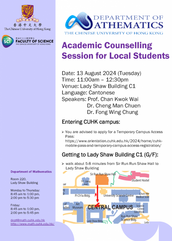](https://www.math.cuhk.edu.hk/sites/default/files/news/20180328_thomas_hou_lecture_poster.pdf)
---
# Former Faculty Members | CUHK Mathematics
[Skip to main content](#main-content)
[](http://www.cuhk.edu.hk "The Chinese University of Hong Kong")
[](http://www.sci.cuhk.edu.hk/ "Faculty of Science")
[](/ "Home")
Search form
-----------
Search Search Search
[](https://imap.math.cuhk.edu.hk "Math Webmail")
[](/user "Login to this Math Web")
1. [Home](/)
2. [People](/people)
3. Former Faculty Members
Former Faculty Members
======================
These scholars of varied mathematical and cultural heritage used to teach, discuss and do mathematics here. Their devotion and memory remain with the many lives they have influenced. We welcome with open arms those who would like to revisit our community, and we miss dearly those who have passed on.
| Name | Period of Service |
| --- | --- |
| [Raymond Honfu CHAN](http://staffweb1.cityu.edu.hk/rhfchan/) | 1993 - 2019 |
| [Ka Sing LAU](mailto:kslau@math.cuhk.edu.hk) | 1996 - 2017 |
| Ping Kwan TAM | 1970 - 2015 |
| Juncheng WEI | 1995 - 2015 |
| [Po Lam YUNG](https://maths-people.anu.edu.au/~plyung/) | 2014 - 2021 |
---
# Zhizhen School of Interdisciplinary Mathematical Sciences 8-Year Articulated Bachelor-Ph.D Programme in Mathematics - Zhizhen School of Interdisciplinary Mathematical Sciences 8-Year Articulated Bachelor-Ph.D Programme in Mathematics
The Chinese University of Hong Kong (CUHK) has established the Zhizhen School of Interdisciplinary Mathematical Sciences (Zhizhen School, or “the School”), as an initiative of internationally renowned mathematician Professor Yau Shing-tung. It aims to cultivate mathematical science talent in Hong Kong, aligning with the national aspiration to building China into a leading country in education, as well as the 14th Five-Year Plan’s vision of strengthening basic research. This also aligns with the aspiration in the Hong Kong Special Administrative Region government’s policy address to develop Hong Kong as an international hub for post-secondary education and establish the “Study in Hong Kong” brand. Professor Yau will serve as the Founding Director of Zhizhen School.

=================================


* Zhizhen School of Interdisciplinary Mathematical Sciences 8-Year Articulated Bachelor-Ph.D Programme in Mathematics
* [Introduction](./?Zhizhen_School_of_Interdisciplinary_Mathematical_Sciences_8-Year_Articulated_Bachelor-Ph.D_Programme_in_Mathematics___Introduction)
* [Mission and Vision](./?Zhizhen_School_of_Interdisciplinary_Mathematical_Sciences_8-Year_Articulated_Bachelor-Ph.D_Programme_in_Mathematics___Mission_and_Vision)
* [Admission and Selection](./?Zhizhen_School_of_Interdisciplinary_Mathematical_Sciences_8-Year_Articulated_Bachelor-Ph.D_Programme_in_Mathematics___Admission_and_Selection)
* [Webinar](./?Zhizhen_School_of_Interdisciplinary_Mathematical_Sciences_8-Year_Articulated_Bachelor-Ph.D_Programme_in_Mathematics___Webinar)
* [Important Dates](./?Zhizhen_School_of_Interdisciplinary_Mathematical_Sciences_8-Year_Articulated_Bachelor-Ph.D_Programme_in_Mathematics___Important_Dates)
* [Contact](./?Zhizhen_School_of_Interdisciplinary_Mathematical_Sciences_8-Year_Articulated_Bachelor-Ph.D_Programme_in_Mathematics___Contact)
X
X
---
# PhD Careers | CUHK Mathematics
[Skip to main content](#main-content)
[](http://www.cuhk.edu.hk "The Chinese University of Hong Kong")
[](http://www.sci.cuhk.edu.hk/ "Faculty of Science")
[](/ "Home")
Search form
-----------
Search Search Search
[](https://imap.math.cuhk.edu.hk "Math Webmail")
[](/user "Login to this Math Web")
1. [Home](/)
2. [People](/people)
3. PhD Careers
PhD Careers
===========
Our PhD graduates have successful careers in both academia and industry. Many of them started out as postdoctoral researchers, while others have entered various industries, making use of their training in mathematical research.
### Academia
Some of our graduates spread the light of education throughout the world as postdoctoral researchers and faculties in different institutes. Here we list graduates who have held postdoctoral and faculty positions locally or abroad:
#### [2021 - Present](#collapse-academia-2021)
#### **2024**
* * *
* **Yan Lung LI**
Senior Researcher, Institute for Basic Science Center for Geometry and Physics (POSTECH Campus)
* * *
#### **2023**
* * *
* **Fuqun HAN**
Hedrick Assistant Adjunct Professor, University of California, Los Angeles
* **Zhongqian WANG**
Postdoctoral Fellow, Technical University of Munich
* **Yu Tung YAU**
Postdoctoral Assistant Professor, University of Michigan
* * *
#### **2022**
* * *
* **Gaoming WANG**
Visiting Assistant Professor, Cornell University
* **Yiran WANG**
Golomb Visiting Assistant Professor, Purdue University
* **Zehui ZHOU**
Hill Assistant Professor, Rutgers University
* * *
#### **2021**
* * *
* **Bowen LI**
Phillip Griffiths Assistant Research Professor, Duke University
* **Ying LIANG**
Golomb Visiting Assistant Professor, Purdue University
* * *
#### [2016 - 2020](#collapse-academia-2016)
#### **2020**
* * *
* **Shanjiang CHEN**
Postdoctoral Fellow, National Center for Theoretical Sciences
* * *
#### **2019**
* * *
* **Xiaoxiang CHAI**
Postdoctoral Fellow, Korea Institute for Advanced Study
* **Simon PUN**
Visiting Assistant Professor, Texas A&M University
* **Zhu ZHANG**
Postdoctoral Fellow, City University of Hong Kong
* * *
#### **2018**
* * *
* **Guanheng CHEN**
Postdoctoral Fellow, University of Adelaide
* **Yuan CHEN**
Postdoctoral Fellow, Michigan State University
* **Qingyuan JIANG**
Postdoctoral Fellow, Institute for Advanced Study, Princeton University
* **Rihuan KE**
Postdoctoral Fellow, University of Cambridge
* **Man-Chun LEE**
Postdoctoral Fellow, University of British Columbia
* **Yat-Hin SUEN**
Postdoctoral Fellow, Institute for Basic Science, Center for Geometry & Physics, Korea
* **Chao WANG**
Postdoctoral Fellow, University of Texas at Dallas
* * *
#### **2017**
* * *
* **Chi Yeung LAM**
Postdoctoral Fellow, Michigan State University
* * *
#### **2016**
* * *
* **Yalong CAO**
Postdoctoral Fellow, Kavli Institute for Physics and Mathematics, University of Tokyo
* **Shaochuang HUANG**
Postdoctoral Fellow, Yau Mathematical Sciences Center, Tsinghua university
* **Jeffery Ka Chun LAM**
Von Karman Postdoctoral Instructorship, California Institute of Technology
* * *
#### [2011 - 2015](#collapse-academia-2011)
#### **2015**
* * *
* **Yat Tin CHOW**
CAM Assistant Professor, University of California, Los Angeles
* * *
#### **2014**
* * *
* **Haixia LIU**
Postdoctoral Fellow, Hong Kong University of Science and Technology
* **Ziming MA**
Postdoctoral Fellow, Harvard University
Assistant Professor, National Taiwan University
* **Guojian YIN**
Postdoctoral Fellow, CAS and Shenzhen Institute of Advanced Technology
* * *
#### **2013**
* * *
* **Kai-leung CHAN**
Postdoctoral Fellow, University of Hong Kong
* **Yunxia CHEN**
Postdoctoral Fellow, University of Bonn and University of Waterloo
* * *
#### **2012**
* * *
* **Xiaohao CAI**
Postdoctoral Fellow, Kaiserslautern University of Technology
* **Chun Kit LAI**
Postdoctoral Fellow, McMaster University
Postdoctoral Fellow, University of Cambridge
* * *
#### **2011**
* * *
* **Kwok Kun KWONG**
Postdoctoral Fellow, Monash University
* **Siu Cheong LAU**
Postdoctoral Fellow, Harvard University and University of Tokyo
Benjamin Peirce Assistant Professor, Harvard University
* **Wei YAO**
Postdoctoral Fellow, Universidad de Chile
* * *
#### [2006 - 2010](#collapse-academia-2006)
#### **2010**
* * *
* **Hai-Xia LIANG**
Postdoctoral Fellow, Nanyang Technological University
* * *
#### **2009**
* * *
* **Jian-Feng CAI**
CAM Assistant Adjunct Professor, University of California, Los Angeles
* **Changzheng LI**
Postdoctoral Fellow, Korea Institute for Advanced Study (KIAS)
* **Jingzhi LI**
Postdoctoral Fellow, ETH Zurich (Swiss Federal Institute of Technology)
* **Wei WANG**
Postdoctoral Fellow, The Chinese Academy of Sciences and Max-Planck Institute Partner Institute of Computational Biology
* * *
#### **2008**
* * *
* **Kwok Wai CHAN**
Postdoctoral Fellow, Harvard University
* **Bangti JIN**
Postdoctoral Fellow, Alexander von Humboldt Fellowship
* **Kai ZHANG**
Postdoctoral Fellow, Michigan State University
* * *
#### **2007**
* * *
* **Jian Feng CAI**
Postdoctoral Fellow, National University of Singapore
* **Yiqiu DONG**
Postdoctoral Fellow, University of Graz
_Co-supervised under CUHK-Beijing University agreement_
* **Yongdong HUANG**
Postdoctoral Fellow, Shanghai East China Normal University
Assistant Professor, Jinan University
* **Guoyin LI**
Postdoctoral Fellow, University of New South Wales
* **Hongyu LIU**
Acting Assistant Professor, University of Washington (Seattle)
* **Yin LE**
Assistant Professor, Shenzhen University
* **Lin SHU**
Postdoctoral Fellow, Peking University
* **Chunjing XIE**
Postdoctoral Fellow, The Chinese University of Hong Kong
* **Jiajin ZHANG**
Postdoctoral Fellow, University of Mainz
* * *
#### **2006**
* * *
* **Dongjuan NIU**
Postdoctoral Fellow, Chinese Academy of Sciences
* **Mao SHENG**
Postdoctoral Fellow, Universitat Mainz
* **Lulin TAN**
Postdoctoral Fellow, Sun Yat-Sen University
* * *
#### [2001 - 2005](#collapse-academia-2001)
#### **2004**
* * *
* **Zheng Jian BAI**
Postdoctoral Fellow, National University of Singapore
* **Kit Hung CHAN**
Postdoctoral Fellow, University of Exeter
* **Jing LI**
Postdoctoral Fellow, Osaka University
* * *
---
# Introductory Lecture of the Shaw Prize Lecture 2023 | CUHK Mathematics
[Skip to main content](#main-content)
[](http://www.cuhk.edu.hk "The Chinese University of Hong Kong")
[](http://www.sci.cuhk.edu.hk/ "Faculty of Science")
[](/ "Home")
Search form
-----------
Search Search Search
[](https://imap.math.cuhk.edu.hk "Math Webmail")
[](/user "Login to this Math Web")
1. [Home](/)
2. [News](/news)
3. Introductory Lecture of the Shaw Prize Lecture 2023
Introductory Lecture of the Shaw Prize Lecture 2023
===================================================
Date Posted:
12 October, 2023
[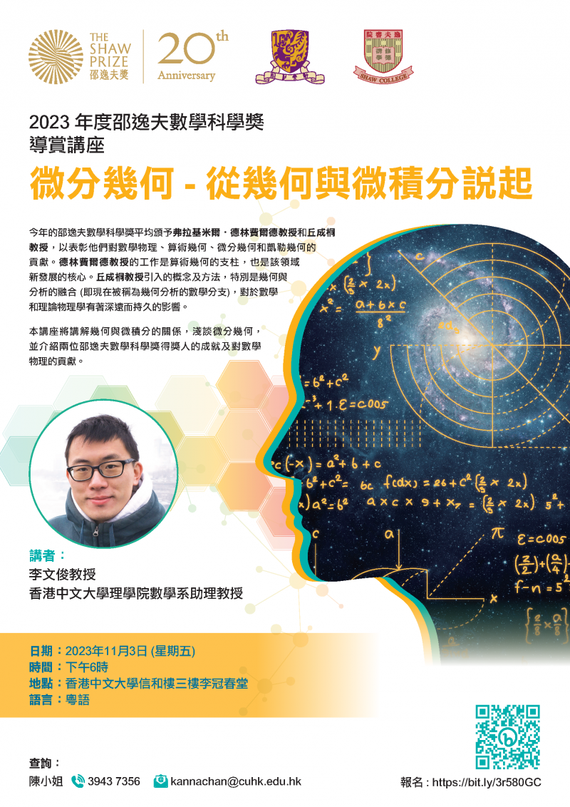](https://www.math.cuhk.edu.hk/sites/default/files/news/20231113_cuhk_the_shaw_prize_lecture.pdf)
---
# The HongKong-Taiwan Joint Conference On Applied Mathematics and Related topics | CUHK Mathematics
[Skip to main content](#main-content)
[](http://www.cuhk.edu.hk "The Chinese University of Hong Kong")
[](http://www.sci.cuhk.edu.hk/ "Faculty of Science")
[](/ "Home")
Search form
-----------
Search Search Search
[](https://imap.math.cuhk.edu.hk "Math Webmail")
[](/user "Login to this Math Web")
1. [Home](/)
2. [News](/news)
3. The HongKong-Taiwan Joint Conference On Applied Mathematics and Related topics
The HongKong-Taiwan Joint Conference On Applied Mathematics and Related topics
==============================================================================
Date Posted:
7 February, 2024
[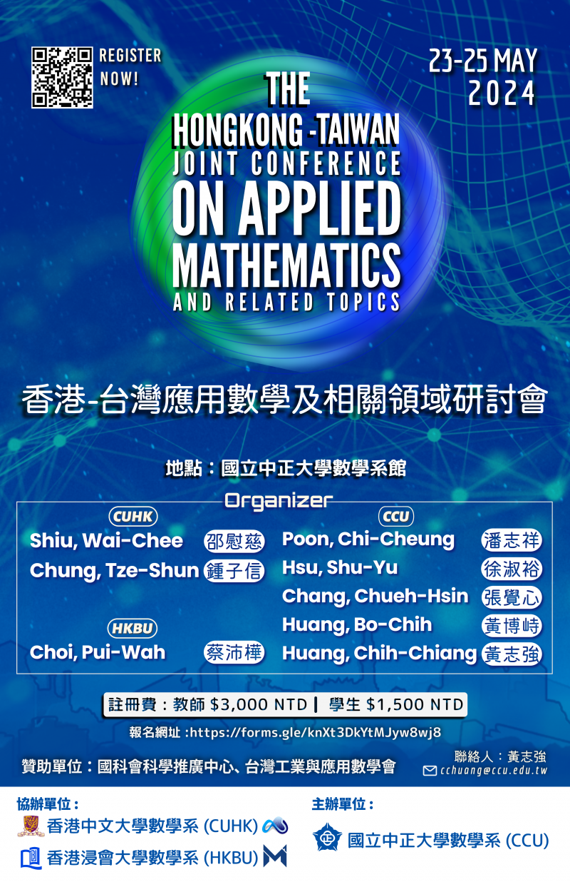](https://www.math.cuhk.edu.hk/sites/default/files/news/20240207-2.png)
---
# Prof. Gary Pui Tung CHOI | CUHK Mathematics
[Skip to main content](#main-content)
[](http://www.cuhk.edu.hk "The Chinese University of Hong Kong")
[](http://www.sci.cuhk.edu.hk/ "Faculty of Science")
[](/ "Home")
Search form
-----------
Search Search Search
[](https://imap.math.cuhk.edu.hk "Math Webmail")
[](/user "Login to this Math Web")
1. [Home](/)
2. [People](/people)
3. [Academic Staff](/people/academic-staff)
4. Prof. Gary Pui Tung CHOI
Prof. Gary Pui Tung CHOI
========================
**Vice-Chancellor Assistant Professor**
_BSc (The Chinese University of Hong Kong)
MPhil (The Chinese University of Hong Kong)
PhD (Harvard University)_
* * *
[![[Teacher's name in full]](https://www.math.cuhk.edu.hk/sites/default/files/resize/people/gary_choi_profile-240x320.png)](https://www.math.cuhk.edu.hk/sites/default/files/people/gary_choi_profile.png)
**ORCID:**
[0000-0001-5407-9111](https://orcid.org/0000-0001-5407-9111)
* * *
**Address:**
Room 204, Lady Shaw Building,
The Chinese University of Hong Kong,
Shatin, N.T., Hong Kong
* * *
**Tel:**
(852) 3943 5481
* * *
**Email:**
[ptchoi@math.cuhk.edu.hk](mailto:ptchoi@math.cuhk.edu.hk)
* * *
**Personal Website:**
[https://www.math.cuhk.edu.hk/~ptchoi/](https://www.math.cuhk.edu.hk/~ptchoi/)
* * *
**Fields of Interest:**
Applied and computational geometry, interdisciplinary mathematical modeling, metamaterial design, quantitative biology, medical imaging, geometry processing, scientific computing
* * *
**Selected Publications:**
1. (with L. H. Dudte, K. P. Becker, and L. Mahadevan) An additive framework for kirigami design. **Nature Computational Science**, 3, 443-454, 2023.
2. (with R. Supekar, B. Song, A. Hastewell, A. Mietke, and J. Dunkel) Learning hydrodynamic equations for active matter from particle simulations and experiments. **Proceedings of the National Academy of Sciences**, 120(7), e2206994120, 2023.
3. (with S. Al-Mosleh, A. Abzhanov, and L. Mahadevan) Geometry and dynamics link form, function and evolution of finch beaks.
**Proceedings of the National Academy of Sciences**, 118(46), e2105957118, 2021.
4. (with L. H. Dudte and L. Mahadevan) An additive algorithm for origami design. **Proceedings of the National Academy of Sciences**, 118(21), e2019241118, 2021.
5. Efficient conformal parameterization of multiply-connected surfaces using quasi-conformal theory. **Journal of Scientific Computing**, 87(3), 70, 2021.
6. (with S. Chen and L. Mahadevan) Deterministic and stochastic control of kirigami topology. **Proceedings of the National Academy of Sciences**, 117(9), 4511-4517, 2020.
7. (with L. H. Dudte and L. Mahadevan) Programming shape using kirigami tessellations. **Nature Materials**, 18(9), 999-1004, 2019.
8. (with A. Pumarola, J. Sanchez-Riera, A. Sanfeliu, and F. Moreno-Noguer) 3DPeople: Modeling the geometry of dressed humans.
**The IEEE International Conference on Computer Vision (ICCV)**, 2242-2251, 2019.
9. (with C. H. Rycroft) Density-equalizing maps for simply connected open surfaces. **SIAM Journal on Imaging Sciences**, 11(2), 1134-1178, 2018.
10. (with K. C. Lam and L. M. Lui) FLASH: Fast landmark aligned spherical harmonic parameterization for genus-0 closed brain surfaces. **SIAM Journal on Imaging Sciences**, 8(1), 67-94, 2015.
* * *
**Honours and Awards:**
* NSF Mathematical Sciences Postdoctoral Research Fellowship, 2020
* New World Mathematics Award, Silver Medal for Master Thesis, 2017
* Croucher Foundation Scholarship, 2016
* Hong Kong Scholarship for Excellence, 2016
* * *
#### Courses
[Current Academic Year](#teacher_current_courses_content)
----------------------------------------------------------
| Course Code | Course Title | Academic Year | Term |
| --- | --- | --- | --- |
| [MATH4400A](/course/2425/math4400a) | [Project](/course/math4400) | 2024/25 | 1 |
| [MATH2221A](/course/2425/math2221a) | [Mathematics Laboratory II](/course/math2221) | 2024/25 | 2 |
| [MATH2221B](/course/2425/math2221b) | [Mathematics Laboratory II](/course/math2221) | 2024/25 | 2 |
| [MATH2221C](/course/2425/math2221c) | [Mathematics Laboratory II](/course/math2221) | 2024/25 | 2 |
[Previous Academic Years](#teacher_previous_courses_content)
-------------------------------------------------------------
| Course Code | Course Title | Academic Year | Term |
| --- | --- | --- | --- |
| [MATH1010F](/course/2324/math1010f) | [University Mathematics](/course/math1010) | 2023/24 | 1 |
---
# Second Major in Mathematics | CUHK Mathematics
[Skip to main content](#main-content)
[](http://www.cuhk.edu.hk "The Chinese University of Hong Kong")
[](http://www.sci.cuhk.edu.hk/ "Faculty of Science")
[](/ "Home")
Search form
-----------
Search Search Search
[](https://imap.math.cuhk.edu.hk "Math Webmail")
[](/user "Login to this Math Web")
1. [Home](/)
2. [Undergraduates](/undergraduates)
3. Second Major in Mathematics
Second Major in Mathematics
===========================
The new undergraduate curriculum offers an extra year for many students to pursue a second major in Mathematics. A single degree indicating two majors will be awarded, the degree being that of the first major. Programmes that have already incorporated sufficient mathematics content will not be eligible to make mathematics a second major. These programmes include BEng Mathematics and Information Engineering and BEd Mathematics and Mathematics Education. Enquiries should be directed to Faculty of Engineering and Faculty of Education correspondingly.
Students with their second major intention endorsed by the Department of Mathematics are eligible for all benefits of mathematics major including scholarships, internships, outgoing research, and other opportunities, together with students from BEng Mathematics and Information Engineering and BEd Mathematics and Mathematics Education. However the prioirty of all these students will be lower than all students with first major in Mathematics.
###
Procedures
* * *
Students who wish to declare a double major must complete the requirements of both majors within the normal period of study and attain the required cumulative grade point average (CGPA).
Students are advised to search for "second major" in [CUHK RES](http://www.cuhk.edu.hk/rgs)
for the most updated procedures, and the application period applicable to the current academic year.
1. With the approval of the first major department and ours, students may declare a second major in Mathematics **at the start of the last term of attendance within the normative study period**.
2. Students can make inquiries to us and express in writing the intention of declaring the second major at least one term before registration of the second major.
* The Department of Mathematics will only consider second major intention from students who have completed 33 units according to the following
* Science Faculty Package (9 units)
* MATH1010, 1030, 1050, 2010, 2020, 2040, 2050, 2070, 2230 (additional 24 units)
* Historically, to complete the above, students with intention for second major in Mathematics at least needed 2.5 years including well use of summer courses.
* The letter of intention should demonstrate an academic plan to complete the second major. The academic plan will be judged with reference to previous academic result.
3. Before making the declaration, students must have attained a CGPA of 3.0 or above in all the courses taken before the last term of attendance. Students must also have completed/registered for all course requirements for graduation purposes in the first major (including Faculty/University/College requirements) at the time the declaration of second major is made.
4. The application form for "Declaration of a Second Major" is obtainable from CUHK RES **within the add/drop period of each term**. Students permitted to declare a second major should submit the approved form to RES by the close of the application period listed in CUHK RES.
5. Students who have declared double major and cannot complete the requirements of the first or second major within the normative study period will be charged a prescribed fee for the remaining units of courses according to the fee schedule on the CUHK RES homepage.
---
# The Taiwan-Hong Kong Joint Conference on Applied Mathematics and Related Topics 2025 | CUHK Mathematics
[Skip to main content](#main-content)
[](http://www.cuhk.edu.hk "The Chinese University of Hong Kong")
[](http://www.sci.cuhk.edu.hk/ "Faculty of Science")
[](/ "Home")
Search form
-----------
Search Search Search
[](https://imap.math.cuhk.edu.hk "Math Webmail")
[](/user "Login to this Math Web")
1. [Home](/)
2. [News](/news)
3. The Taiwan-Hong Kong Joint Conference on Applied Mathematics and Related Topics 2025
The Taiwan-Hong Kong Joint Conference on Applied Mathematics and Related Topics 2025
====================================================================================
Date Posted:
20 January, 2025
[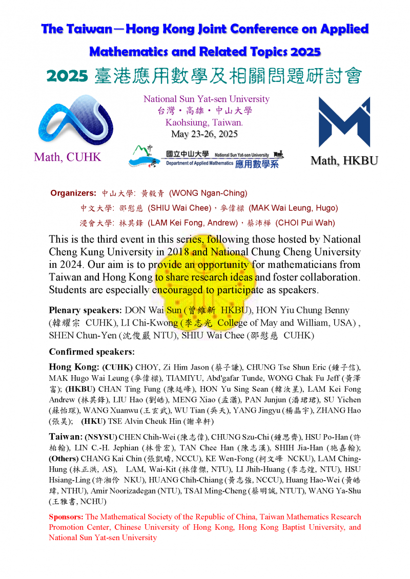](https://www-math.nsysu.edu.tw/~wong/taiwan-HK2025/)
[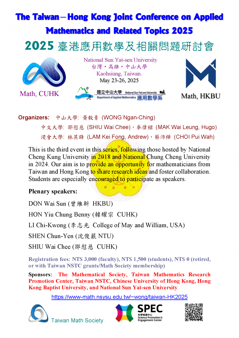](https://www-math.nsysu.edu.tw/~wong/taiwan-HK2025/)
---
# Prof. Eric Tsz Shun CHUNG | CUHK Mathematics
[Skip to main content](#main-content)
[](http://www.cuhk.edu.hk "The Chinese University of Hong Kong")
[](http://www.sci.cuhk.edu.hk/ "Faculty of Science")
[](/ "Home")
Search form
-----------
Search Search Search
[](https://imap.math.cuhk.edu.hk "Math Webmail")
[](/user "Login to this Math Web")
1. [Home](/)
2. [People](/people)
3. [Academic Staff](/people/academic-staff)
4. Prof. Eric Tsz Shun CHUNG
Prof. Eric Tsz Shun CHUNG
=========================
**Professor**
_BSc, MPhil (The Chinese University of Hong Kong)
PhD (University of California, Los Angeles)_
* * *
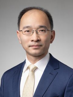
**ORCID:**
[0000-0002-3096-3399](https://orcid.org/0000-0002-3096-3399)
* * *
**Address:**
Room 205, Lady Shaw Building,
The Chinese University of Hong Kong,
Shatin, N.T., Hong Kong
* * *
**Tel:**
(852) 3943 7972
* * *
**Email:**
[tschung@math.cuhk.edu.hk](mailto:tschung@math.cuhk.edu.hk)
* * *
**Personal Website:**
[http://www.math.cuhk.edu.hk/~tschung/](http://www.math.cuhk.edu.hk/~tschung/)
* * *
**Fields of Interest:**
Multiscale methods for high-contrast multiscale flow and wave problems, Multiscale model reduction for fractured media and perforated domains, Nonlinear upscaling methods for nonlinear heterogeneous problems, Data driven multiscale model reduction, Machine learning based reduced order modelling, Discontinuous Galerkin methods: theory, numerics and applications, Domain decomposition methods for multiscale problems, Applications of advanced numerical methods in the geosciences
* * *
**Selected Publications:**
1. Yiran Wang, Eric Chung and Shubin Fu.
A local-global generalized multiscale finite element method for highly heterogeneous stochastic groundwater flow problems. Computer Methods in Applied Mechanics and Engineering, 392 (2022), 114688.
2. Lina Zhao, Dohyun Kim, Eun-Jae Park and Eric Chung.
Staggered DG method with small edges for Darcy flows in fractured porous media. Journal of Scientific Computing, 90 (2022).
3. Yating Wang, Siu Wun Cheung, Eric T. Chung, Yalchin Efendiev and Min Wang.
Deep multiscale model learning. Journal of Computational Physics, 406 (2020), 109071.
4. Eric Chung, Yalchin Efendiev and Wing Tat Leung.
Constraint energy minimizing generalized multiscale finite element method. Computer Methods in Applied Mechanics and Engineering, 339 (2018), pp. 298-319
5. Eric Chung, Yalchin Efendiev and Thomas Y. Hou.
Adaptive multiscale model reduction with generalized multiscale finite element methods. Journal of Com- putational Physics, 320 (2016), pp. 69-95.
* * *
**Major Research Grants:**
* Research Grants Council - General Research Fund
* Germany Academic Exchange Service and Research Grant Council - Joint Research Scheme
* * *
**Honours and Awards:**
* ICCM Silver Medal of Mathematics
* Outstanding Fellow of the Faculty of Science
* Hong Kong Mathematical Society Young Scholar Award
* * *
**Professional activities:**
* RGC Physical Science Panel
* Membership Committee, Society for Industrial and Applied Mathematics
**Editorial board:**
* Specialty Chief Editor (since March 2022), Frontier in Applied Mathematics and Statistics
* Editorial Board (since August 2020), Mathematical and Computational Applications
* Editorial Board (since August 2020), Taiwanese Journal of Mathematics
* Editorial Board (since August 2020), Mathematics and Computers in Simulation
* Editorial Board (since January 2018), Computers & Mathematics with Applications
* Editorial Board (since April 2011), Journal of Computational and Applied Mathematics
* * *
#### Courses
[Current Academic Year](#teacher_current_courses_content)
----------------------------------------------------------
| Course Code | Course Title | Academic Year | Term |
| --- | --- | --- | --- |
| [MATH4280](/course/2425/math4280) | [Innovation and Design in Big Data Analytics](/course/math4280) | 2024/25 | 1 |
| [MATH5212](/course/2425/math5212) | [Advanced Numerical Analysis II](/course/math5212) | 2024/25 | 1 |
| [MMAT5320](/course/2425/mmat5320) | [Computational Mathematics](/course/mmat5320) | 2024/25 | 1 |
| [MATH6212](/course/2425/math6212) | [Topics in Applied Mathematics II](/course/math6212) | 2024/25 | 2 |
[Previous Academic Years](#teacher_previous_courses_content)
-------------------------------------------------------------
| Course Code | Course Title | Academic Year | Term |
| --- | --- | --- | --- |
| [MATH4280](/course/2324/math4280) | [Innovation and Design in Big Data Analytics](/course/math4280) | 2023/24 | 1 |
| [MATH5211](/course/2324/math5211) | [Advanced Numerical Analysis I](/course/math5211) | 2023/24 | 1 |
| [MMAT5320](/course/2324/mmat5320) | [Computational Mathematics](/course/mmat5320) | 2023/24 | 1 |
| [MATH6212](/course/2324/math6212) | [Topics in Applied Mathematics II](/course/math6212) | 2023/24 | 2 |
| [MATH4280](/course/2223/math4280) | [Innovation and Design in Big Data Analytics](/course/math4280) | 2022/23 | 1 |
| [MATH5212](/course/2223/math5212) | [Advanced Numerical Analysis II](/course/math5212) | 2022/23 | 1 |
| [MMAT5270](/course/2223/mmat5270) | [Introduction to Inverse Problems](/course/mmat5270) | 2022/23 | 1 |
| [MATH4280](/course/2122/math4280) | [Innovation and Design in Big Data Analytics](/course/math4280) | 2021/22 | 1 |
| [MATH5211](/course/2122/math5211) | [Advanced Numerical Analysis I](/course/math5211) | 2021/22 | 1 |
| [MMAT5320](/course/2122/mmat5320) | [Computational Mathematics](/course/mmat5320) | 2021/22 | 1 |
| [MATH3290](/course/2122/math3290) | [Mathematical Modeling](/course/math3290) | 2021/22 | 2 |
| [MATH4280](/course/2021/math4280) | [Innovation and Design in Big Data Analytics](/course/math4280) | 2020/21 | 1 |
| [MATH5212](/course/2021/math5212) | [Advanced Numerical Analysis II](/course/math5212) | 2020/21 | 1 |
| [MMAT5320](/course/2021/mmat5320) | [Computational Mathematics](/course/mmat5320) | 2020/21 | 1 |
| [MATH5211](/course/1920/math5211) | [Advanced Numerical Analysis I](/course/math5211) | 2019/20 | 1 |
| [MATH6221](/course/1920/math6221) | [Topics in Numerical Analysis I](/course/math6221) | 2019/20 | 2 |
| [MATH3290](/course/1819/math3290) | [Mathematical Modeling](/course/math3290) | 2018/19 | 1 |
| [MATH5212](/course/1819/math5212) | [Advanced Numerical Analysis II](/course/math5212) | 2018/19 | 1 |
| [MMAT5320](/course/1819/mmat5320) | [Computational Mathematics](/course/mmat5320) | 2018/19 | 1 |
| [MATH3230B](/course/1819/math3230b) | [Numerical Analysis](/course/math3230) | 2018/19 | 2 |
| [MATH3290](/course/1718/math3290) | [Mathematical Modeling](/course/math3290) | 2017/18 | 1 |
| [MATH5211](/course/1718/math5211) | [Advanced Numerical Analysis I](/course/math5211) | 2017/18 | 1 |
| [MMAT5270](/course/1718/mmat5270) | [Introduction to Inverse Problems](/course/mmat5270) | 2017/18 | 1 |
| [MATH3290](/course/1617/math3290) | [Mathematical Modeling](/course/math3290) | 2016/17 | 1 |
| [MATH5212](/course/1617/math5212) | [Advanced Numerical Analysis II](/course/math5212) | 2016/17 | 1 |
| [MATH3290](/course/1516/math3290) | [Mathematical Modeling](/course/math3290) | 2015/16 | 1 |
| [MATH5211](/course/1516/math5211) | [Advanced Numerical Analysis I](/course/math5211) | 2015/16 | 1 |
| [MATH3310](/course/1516/math3310) | [Computational and Applied Mathematics](/course/math3310) | 2015/16 | 2 |
| [MATH3290](/course/1415/math3290) | [Mathematical Modeling](/course/math3290) | 2014/15 | 1 |
| [MATH5212](/course/1415/math5212) | [Advanced Numerical Analysis II](/course/math5212) | 2014/15 | 1 |
| [MMAT5430](/course/1415/mmat5410) | [Graduate Seminar I](/course/mmat5430) | 2014/15 | 1 |
| [MATH3240](/course/1415/math3240) | [Numerical Methods for Differential Equations](/course/math3240) | 2014/15 | 2 |
---
# Prof. Yi Jen LEE | CUHK Mathematics
[Skip to main content](#main-content)
[](http://www.cuhk.edu.hk "The Chinese University of Hong Kong")
[](http://www.sci.cuhk.edu.hk/ "Faculty of Science")
[](/ "Home")
Search form
-----------
Search Search Search
[](https://imap.math.cuhk.edu.hk "Math Webmail")
[](/user "Login to this Math Web")
1. [Home](/)
2. [People](/people)
3. [Academic Staff](/people/academic-staff)
4. Prof. Yi Jen LEE
Prof. Yi Jen LEE
================
**Si Yuan Professor of Mathematics**
_BS (National Taiwan University)
MA, PhD (Harvard University)_
* * *

**Address:**
Room 412, Academic Building No.1,
The Chinese University of Hong Kong,
Shatin, N.T., Hong Kong
* * *
**Tel:**
(852) 3943 3715
* * *
**Email:**
[yjlee@math.cuhk.edu.hk](mailto:yjlee@math.cuhk.edu.hk)
* * *
**Fields of Interest:**
Gauge Theory and Symplectic Topology (e.g. Seiberg-Witten theory), Heegaard Floer Homology and Pseudo-Holomorphic Curves
* * *
#### Courses
[Current Academic Year](#teacher_current_courses_content)
----------------------------------------------------------
| Course Code | Course Title | Academic Year | Term |
| --- | --- | --- | --- |
| [MATH1520B](/course/2425/math1520b) | [University Mathematics for Applications](/course/math1520) | 2024/25 | 1 |
| [MATH4400D](/course/2425/math4400d) | [Project](/course/math4400) | 2024/25 | 1 |
| [MATH4900A](/course/2425/math4900a) | [Seminar](/course/math4900) | 2024/25 | 1 |
| [MATH6072](/course/2425/math6072) | [Topics in Topology II](/course/math6072) | 2024/25 | 2 |
[Previous Academic Years](#teacher_previous_courses_content)
-------------------------------------------------------------
| Course Code | Course Title | Academic Year | Term |
| --- | --- | --- | --- |
| [MATH6071](/course/2324/math6071) | [Topics in Topology I](/course/math6071) | 2023/24 | 1 |
| [MATH6072](/course/2324/math6072) | [Topics in Topology II](/course/math6072) | 2023/24 | 2 |
| [MATH1030D](/course/2223/math1030d) | [Linear Algebra I](/course/math1030) | 2022/23 | 2 |
| [MATH6071](/course/2223/math6071) | [Topics in Topology I](/course/math6071) | 2022/23 | 2 |
| [MATH1520A](/course/2122/math1520a) | [University Mathematics for Applications](/course/math1520) | 2021/22 | 1 |
| [MATH1520AB](/course/2122/math1520ab) | [University Mathematics for Applications](/course/math1520) | 2021/22 | 1 |
| [MATH1520B](/course/2122/math1520b) | [University Mathematics for Applications](/course/math1520) | 2021/22 | 1 |
| [MATH6071](/course/2122/math6071) | [Topics in Topology I](/course/math6071) | 2021/22 | 2 |
| [MATH4900D](/course/2021/math4900d) | [Seminar](/course/math4900) | 2020/21 | 1 |
| [MATH4900E](/course/2021/math4900e) | [Seminar](/course/math4900) | 2020/21 | 1 |
| [MATH1520C](/course/2021/math1520c) | [University Mathematics for Applications](/course/math1520) | 2020/21 | 2 |
| [MATH4900E](/course/1920/math4900e) | [Seminar](/course/math4900) | 2019/20 | 1 |
| [MATH1520C](/course/1920/math1520c) | [University Mathematics for Applications](/course/math1520) | 2019/20 | 2 |
| [MATH6071A](/course/1718/math6071a) | [Topics in Topology I](/course/math6071) | 2017/18 | 1 |
| [MATH6072A](/course/1718/math6072a) | [Topics in Topology II](/course/math6072) | 2017/18 | 2 |
| [MATH6071A](/course/1617/math6071a) | [Topics in Topology I](/course/math6071) | 2016/17 | 1 |
| [MATH6072A](/course/1617/math6072a) | [Topics in Topology II](/course/math6072) | 2016/17 | 2 |
| [MATH6071A](/course/1516/math6071a) | [Topics in Topology I](/course/math6071) | 2015/16 | 1 |
| [MATH6072A](/course/1516/math6072a) | [Topics in Topology II](/course/math6072) | 2015/16 | 2 |
| [MATH5070](/course/1415/math5070) | [Topology of Manifolds](/course/math5070) | 2014/15 | 1 |
| [MATH3423D](/course/1415/math3423d) | [Seminar II](/course/math3423) | 2014/15 | 2 |
| [MATH6071A](/course/1415/math6071a) | [Topics in Topology I](/course/math6071) | 2014/15 | 2 |
---
# Prof. Dejun FENG | CUHK Mathematics
[Skip to main content](#main-content)
[](http://www.cuhk.edu.hk "The Chinese University of Hong Kong")
[](http://www.sci.cuhk.edu.hk/ "Faculty of Science")
[](/ "Home")
Search form
-----------
Search Search Search
[](https://imap.math.cuhk.edu.hk "Math Webmail")
[](/user "Login to this Math Web")
1. [Home](/)
2. [People](/people)
3. [Academic Staff](/people/academic-staff)
4. Prof. Dejun FENG
Prof. Dejun FENG
================
**Professor**
_BEng (Chengdu UST)
PhD (Wuhan University)_
* * *

**Address:**
Room 211, Lady Shaw Building,
The Chinese University of Hong Kong,
Shatin, N.T., Hong Kong
* * *
**Tel:**
(852) 3943 7965
* * *
**Email:**
[djfeng@math.cuhk.edu.hk](mailto:djfeng@math.cuhk.edu.hk)
* * *
**Personal Website:**
[http://www.math.cuhk.edu.hk/~djfeng/](http://www.math.cuhk.edu.hk/~djfeng/)
* * *
**Fields of Interest:**
Fractal Geometry, Ergodic Theory, Dynamical Systems.
* * *
**Selected Publications:**
1. Dimension of invariant measures for affine iterated function systems. Preprint, 2019. To appear in Duke Math. J.
2. Dimension estimates for $C^1$ iterated function systems and repellers. Part II. To appear in Ergodic theory Dynam. Systems (with Karoly Simon)
3. Dimension estimates for $C^1$ iterated function systems and repellers. Part I. To appear in Ergodic theory Dynam. Systems (with Karoly Simon)
4. Estimates on the dimension of self-similar measures with overlaps. To appear in J. Lond. Math. Soc. (with Zhou Feng)
5. On arithmetic sums of fractal sets in ${\\Bbb R}^d$. J. Lond. Math. Soc. 104(2021), no. 1, 35-65. (with Yufeng Wu)
* * *
**Major Research Grants:**
* Research Grants Council - General Research Fund
* * *
**Honours and Awards:**
* Faculty Exemplary Teaching Award
* * *
**Professional activities:**
* Editorial Board - Methods and Applications of Analysis
* * *
#### Courses
[Current Academic Year](#teacher_current_courses_content)
----------------------------------------------------------
| Course Code | Course Title | Academic Year | Term |
| --- | --- | --- | --- |
| [MATH5011](/course/2425/math5011) | [Real Analysis I](/course/math5011) | 2024/25 | 1 |
| [MATH4400K](/course/2425/math4400k) | [Project](/course/math4400) | 2024/25 | 2 |
| [MATH6082](/course/2425/math6082) | [Topics in Analysis II](/course/math6082) | 2024/25 | 2 |
[Previous Academic Years](#teacher_previous_courses_content)
-------------------------------------------------------------
| Course Code | Course Title | Academic Year | Term |
| --- | --- | --- | --- |
| [MATH3280A](/course/2324/math3280a) | [Introductory Probability](/course/math3280) | 2023/24 | 1 |
| [MATH5011](/course/2324/math5011) | [Real Analysis I](/course/math5011) | 2023/24 | 1 |
| [MATH3093](/course/2324/math3093) | [Fourier Analysis](/course/math3093) | 2023/24 | 2 |
| [MATH3280A](/course/2223/math3280a) | [Introductory Probability](/course/math3280) | 2022/23 | 1 |
| [MATH5011](/course/2223/math5011) | [Real Analysis I](/course/math5011) | 2022/23 | 1 |
| [MATH6261](/course/2223/math6261) | [Topics in Probability Theory](/course/math6261) | 2022/23 | 2 |
| [MATH3280A](/course/2122/math3280a) | [Introductory Probability](/course/math3280) | 2021/22 | 1 |
| [MATH5011](/course/2122/math5011) | [Real Analysis I](/course/math5011) | 2021/22 | 1 |
| [MATH3093](/course/2122/math3093) | [Fourier Analysis](/course/math3093) | 2021/22 | 2 |
| [MATH3280](/course/2021/math3280) | [Introductory Probability](/course/math3280) | 2020/21 | 1 |
| [MATH5011](/course/2021/math5011) | [Real Analysis I](/course/math5011) | 2020/21 | 1 |
| [MATH3280](/course/1920/math3280) | [Introductory Probability](/course/math3280) | 2019/20 | 1 |
| [MATH5011](/course/1920/math5011) | [Real Analysis I](/course/math5011) | 2019/20 | 1 |
| [MATH3093](/course/1920/math3093) | [Fourier Analysis](/course/math3093) | 2019/20 | 2 |
| [MATH3280](/course/1819/math3280) | [Introductory Probability](/course/math3280) | 2018/19 | 1 |
| [MATH5011](/course/1819/math5011) | [Real Analysis I](/course/math5011) | 2018/19 | 1 |
| [MATH6081](/course/1819/math6081) | [Topics in Analysis I](/course/math6081) | 2018/19 | 2 |
| [MATH3280](/course/1718/math3280) | [Introductory Probability](/course/math3280) | 2017/18 | 1 |
| [MATH5011](/course/1718/math5011) | [Real Analysis I](/course/math5011) | 2017/18 | 1 |
| [MATH3093](/course/1718/math3093) | [Fourier Analysis](/course/math3093) | 2017/18 | 2 |
| [MATH3280](/course/1617/math3280) | [Introductory Probability](/course/math3280) | 2016/17 | 1 |
| [MATH4900B](/course/1617/math4900b) | [Seminar](/course/math4900) | 2016/17 | 1 |
| [MATH5011](/course/1617/math5011) | [Real Analysis I](/course/math5011) | 2016/17 | 1 |
| [MATH3280A](/course/1516/math3280a) | [Introductory Probability](/course/math3280) | 2015/16 | 1 |
| [MATH4900A](/course/1516/math4900a) | [Seminar](/course/math4900) | 2015/16 | 1 |
| [MATH6081A](/course/1516/math6081a) | [Topics in Analysis I](/course/math6081) | 2015/16 | 1 |
| [MATH3093](/course/1516/math3093) | [Fourier Analysis](/course/math3093) | 2015/16 | 2 |
| [MATH1520A](/course/1415/math1520a) | [University Mathematics for Applications](/course/math1520) | 2014/15 | 1 |
| [MATH3093](/course/1415/math3093) | [Fourier Analysis](/course/math3093) | 2014/15 | 1 |
---
# Unknown
Mathematics Programme Introduction Curriculum There is both breadth and depth to our curriculum. Students can choose from a wide range of courses according to their interests, abilities, and career aspirations. Students majoring in math can graduate in one of our 7 streams of study. For instance, the Enrichment Stream is specially designed to train professional mathematicians, while the Computational and Applied Mathematics (CAM) Stream and Computational Big Data Analytics Stream further increase the breadth of knowledge and emphasizes the ability to apply mathematics for real life problems. Students are required to complete the following courses: 9 units from the Science Faculty Package; 35 units of fundamental Mathematics courses; and 27 units of elective courses Further information is available on the department website: https://www.math.cuhk.edu.hk/undergraduates/streams COSINE China and Overseas Study, Internship and Exchange Program In developing our students' potential, we have organized summer research, work and exchange opportunities under various names since the founding of the Department. Competition for placement is fierce, so ask questions and get prepared early. Our advisors are very willing to help you make the most out of your mathematical studies, so that you could keep a good track record for the career path you would like to pursue. In general, students with good conduct and academic records are eligible to apply. Successful applicants may apply for financial support for summer programmes outside Hong Kong. Past Opportunities Summer Research 1. Caltech (in USA) 2. The Chinese University of Hong Kong 3. Cornell University (in USA) 4. Johns Hopkins Medical School (in USA) 5. Oak Ridge National Laboratory (in USA) 6. Shanghai Institute of Biological Sciences (in China) 7. University of Chicago (in USA) 8. University of Delaware (in USA) 9. University of California, Irvine (in USA) 10. University of California, Los Angeles (in USA) 11. University of Waterloo (in Canada) 12. University System of Taiwan Summer Schools and Workshops 1. Yau Mathematical Sciences Center (YMSC) in Tsinghua University 2. Institute of Mathematics, Academia Sinica (in Taipei) 3. 應用數學暑期學校,北京大學 4. 非線性偏微分方程暑期講習班 5. The International Congress of Chinese Mathematicians (ICCM) 2019 in Tsinghua University 6. 2018年數學拔尖學生聯合暑期學校, 廈門大學 7. 2018國際人工智能暑期學校,哈爾濱 工業大學 Industrial Internship Opportunities 1. Celestial Asia Securities Holdings Limited (CASH Group) Research analyst in algorithmic trading team Business development of mobile trading services 2. ClusterTech Limited Summer intern at advanced clustering technologies team 3. Silverhorn Investment Advisors Limited Summer intern Educational Internship Opportunities 1. Times Publishing (Hong Kong) Limited Textbook editors 2. Hong Kong Educational Publishing Company Textbook editors 3. The Commercial Press (Hong Kong) Ltd. Editorial assistant 4. CCC Mong Man Wai College Classroom teaching positions 5. Christ College Classroom teaching positions 6. Li Kau Yan Memorial School Classroom teaching positions Scholarships On average, more than 80 Mathematics Scholarships (amounting to more than 1 million dollars) are awarded each year, including: 1978 Mathematics Alumus Li Sze-lim Scholarships Department of Mathematics Exemplary Student Award Dr. Chao Yong Chi-hsing Mathematics Scholarship Student Development Scholarship for Mathematics Undergraduates Undergraduate Mathematics Scholarship Details of Department Scholarships are posted under Scholarships on the department website. Career Path On completion of this degree, graduates should have acquired good mathematical knowledge and skills for their further studies and/or careers. Recent past graduates have started careers in professions including: Banking Computer Science Data Science Engineering Education Information Technology Quantitative Finance Further studies Every year, a significant proportion of our graduates pursue further studies abroad, in prestigious graduate programmes such as those at the following universities: Princeton University Harvard University Massachusetts Institute of Technology University of California, Berkeley Stanford University University of Cambridge University of Oxford They are typically fully supported in these programmes through scholarships, fellowships and teaching assistantships. Department of Mathematics, Room 220, Lady Shaw Building, The Chinese University of Hong Kong Tel: 39437988 Fax: 26035154 Email: dept@math.cuhk.edu.hk Website: https://www.math.cuhk.edu.hk/
---
# Unknown
Weekly Inverse Problems at CUHK
Schedule of Fall 2022
**December 1, [Kuang Huang](https://cm3.apam.columbia.edu/people/kuang-huang)
(Columbia University) [poster](seminar/S221201_Inverse%20Problems%20Seminar.pdf)
**
**November 24, [Markus Haltmeier](https://applied-math.uibk.ac.at/index.php/members/scientific-staff/markus-haltmeier)
(University of Innsbruck) [poster](seminar/S221124_Inverse%20Problems%20Seminar.pdf)
**
**November 17, [Christian Clason](https://homepage.uni-graz.at/de/c.clason/)
(University of Graz) [poster](seminar/S221117_Inverse%20Problems%20Seminar.pdf)
**
**November 10, [Erik Burman](https://iris.ucl.ac.uk/iris/browse/profile?upi=ENBUR31)
(University College London) [poster](seminar/S221110_Inverse%20Problems%20Seminar.pdf)
**
**November 3, [Qianxiao Li](https://blog.nus.edu.sg/qianxiaoli/)
(National University of Singapore) [poster](seminar/S221103_Inverse%20Problems%20Seminar.pdf)
**
**October 27, [Lei Zhang](https://ins.sjtu.edu.cn/people/lzhang/)
(Shanghai Jiaotong University) [poster](seminar/S221027_Inverse%20Problems%20Seminar.pdf)
**
**October 20, [Elen Beretta](https://sites.google.com/view/eberetta/home)
(NYU Abu Dhabi) [poster](seminar/S221020_Inverse%20Problems%20Seminar.pdf)
(cancelled)**
**October 13, [Kui Ren](http://www.columbia.edu/~kr2002/)
(Columbia University) [poster](seminar/S221013_Inverse%20Problems%20Seminar.pdf)
**
**October 6, [Shuai Lu](https://homepage.fudan.edu.cn/shuailu/)
(Fudan University)** **[poster](seminar/S221006_Inverse%20Problems%20Seminar.pdf)
**
**September 29, [Xiliang Lu](seminar)
(Wuhan University)** **[poster](seminar/S220929_Inverse%20Problems%20Seminar.pdf)
**
**September 8, [Xin Tong](https://sites.google.com/view/xintongthomson/home)
(National University of Singapore) [poster](seminar/S220908_Inverse%20Problems%20Seminar.pdf)
**
**August 12, [Xudong Chen](https://www.ece.nus.edu.sg/stfpage/elechenx/)
(National University of Singapore)** [poster](seminar/S220812_Xudong%20Chen.pdf)
**August 11, [Xudong Chen](https://www.ece.nus.edu.sg/stfpage/elechenx/)
(National University of Singapore)** [poster](seminar/S220811_Xudong%20Chen.pdf)
�
---
# Unknown
We are constantly looking for **highly motivated students with strong mathematical background and / or programming skills** to join the research group of Prof. Bangti Jin, at Department of Mathematics, The Chinese University of Hong Kong. The group currently has the following open positions: research assistant professor, PhD position, research assistant / MPhi students. Interested candidates are cordially invited to apply for the positions directly via emailing the relevant materials (cv, transcripts, expression of interest) to Prof. Bangti Jin (b.jin@cuhk.edu.hk).
===========================================================================================================================================================================================================================================================================================================================================================================================================================================================================================================================================================================================
**One position of research assistant professor** at Department of Mathematics, The Chinese University of Hong Kong. The details can be found at [https://www.math.cuhk.edu.hk/about-us/job-opportunities](https://www.math.cuhk.edu.hk/about-us/job-opportunities)
. Please apply through mathjob.org: [https://www.mathjobs.org/jobs/list/22310](https://www.mathjobs.org/jobs/list/22310)
**One PhD position on deep solvers for PDEs** (jointly with Prof. Simon Arridge, Department of Computer Science University College London).
The studentship is funded by the international joint supervision of PhD students scheme of CUHK. The project is to investigate deep neural networks for solving inverse problems associated with partial differential equations, with a focus on developing efficient numerical algorithms and / or establishing theoretical guarantees. The specific inverse problems of interest include electrical impedance tomography, current density impedance imaging and conductivity imaging from partial interior data. The topics deal with the development and application of neural networks and their integration to inverse problems, and the main tasks of the student include (but not limited to): 1) conduct numerical experiments on model inverse problems; 2) conduct preliminary theoretical analysis of the algorithm, e.g., generalization error analysis; 3) perform comparative study with traditional methods. The deadline for the application is September 20, 2023, and the application and questions on the position should be sent directly to Bangti Jin (b.jin@cuhk.edu.hk).
**Two research assistant / MPhil** **student** **positions** in computational inverse problems / numerical analysis broadly speaking. Potential topics of interest include but not limited to:
(1) theoretical and applied aspects of adaptive FEM for PDE constrained optimization
(2) neural networks for solving PDEs
(3) stochastic iterative methods
(4) generative models for inverse problems etc.
---
# Unknown
**MATH6221 (fall 2023), Topics in Numerical Analysis**
Instructor: Bangti Jin ([b.jin@cuhk.edu.hk](mailto:b.jin@cuhk.edu.hk)
)
Lecture room: Lady Shaw Building 222
Lecture hour: 9:30 am � 12:15 pm
Important note: The first lecture will be on Sept. 9, Saturday (instead of Sept. 4, Monday).
Lecture slide
Week 13, December 4, No lecture, presentation for final assessment
Week 12, November 27, [lect11](math6221/lect11.pdf)
Week 11, November 20, [lect10](math6221/lect10.pdf)
Week 10, November 13, [lect9](math6221/lect9.pdf)
Week 9, November 6, [lect8](math6221/lect8.pdf)
Week 8, October 30, [lect7](math6221/lect7.pdf)
Week 7, October 23, [lect6](math6221/lect6.pdf)
Week 6, October 9, [lect5](math6221/lect5.pdf)
Week 5 (cancelled for holiday)
Week 4, September 25 [lect4](math6221/lect4.pdf)
Week 3, September 18 [lect3](math6221/lect3.pdf)
Week 2, September 11 [lect2](math6221/lect2.pdf)
Week 1, September 9 [lect1](math6221/lect1.pdf)
The first part of the lectures is based on standard references, e.g.,
1. C. Vogel. Computational Methods for Inverse Problems, SIAM 2002
2. H. Engl, M. Hanke, A. Neubauer. Regularization of Inverse Problems, Kluwer, 1996
3. K. Ito, B. Jin. Inverse Problems: Tikhonov Theory and Algorithms, World Scientific, 2015
4. P. Hansen. Rank-Deficient and Discrete Ill-Posed Problems, SIAM, 1998
The second part of the lectures will be based on recent papers and reviews, and will be posted accordingly.
The following papers are possible materials for presentation:
[Paper1](math6221/p1.pdf)
[paper2](math6221/p2.pdf)
[paper3](math6221/p3.pdf)
[paper4](math6221/lect4.pdf)
[paper5](math6221/p5.pdf)
[paper6](math6221/p6.pdf)
[paper7](math6221/p7.pdf)
[paper8](math6221/p8.pdf)
[paper9](math6221/p9.pdf)
---
# Publications
****
The most updated publication list is available from [Google Scholar](https://scholar.google.com/citations?hl=en&user=8Axgx3wAAAAJ&view_op=list_works&sortby=pubdate)
page.
**Monographs:**
****
1. Kazufumi Ito, Bangti Jin. Inverse Problems: Tikhonov Theory and Algorithms, World Publishing, 2014. [publisher](http://www.worldscientific.com/worldscibooks/10.1142/9120)
, [Amazon](http://www.amazon.com/Inverse-Problems-Tikhonov-Theory-Algorithms/dp/9814596191/ref=sr_1_1?s=books&ie=UTF8&qid=1415802802&sr=1-1&keywords=kazufumi+ito)
2. Bangti Jin. Fractional Differential Equations. (Applied Mathematical Sciences, vol. 206). Springer 2021. [publisher](https://link.springer.com/book/10.1007/978-3-030-76043-4)
, [Amazon](https://www.amazon.com/Fractional-Differential-Equations_-An-Approach-via-Fractional-Derivatives-_Applied-Mathematical-Sciences-Book-206_/dp/B09B38PMCJ)
3. Bangti Jin, Zhi Zhou. Numerical Treatment and Analysis of Time-Fractional Evolution Equations (Applied Mathematical Sciences, vol. 214). Springer 2023. [publisher](https://link.springer.com/book/9783031210495)
**Journal articles**:
**2023**
1. Siyu Cen, Bangti Jin, Qimeng Quan, Zhi Zhou. Hybrid neural-network FEM approximation of diffusion coefficient in elliptic and parabolic problems. IMA Journal of Numerical Analysis, in press.
2. Siyu Cen, Bangti Jin, Kwancheol Shin, Zhi Zhou. Deep Calderon method for electrical impedance tomography. Journal of Computational Physics, in press.
3. Siyu Cen, Bangti Jin, Yikan Liu, Zhi Zhou. Recovery of multiple parameters in subdiffusion from one lateral boundary measurement. Inverse Problems, in press.
4. Tianhao Hu, Bangti Jin, Zhi Zhou. Solving elliptic problems with singular sources using singularity splitting deep Ritz method. SIAM Journal on Scientific Computing 2023; 45 (4): 2043--2074.
5. Bangti Jin, Yavar Kian, Zhi Zhou. Inverse problems for subdiffusion from observation at an unknown terminal time. SIAM Journal on Applied Mathematics 2023; 83 (4): 1496-1517.
6. Bangti Jin, Zeljko Kereta. On the convergence of stochastic gradient descent for linear inverse problems in Banach spaces. SIAM Journal on Imaging Sciences 2023; 16 (2): 671-705.
7. Bangti Jin, Yavar Kian. Recovery of a distributed order fractional derivative in an unknown medium. Communications in Mathematical Sciences, in press.
8. Riccardo Barbano, Johannes Leuschner, Maximilian Schmidt, Alexander Denker, Andreas Hauptmann, Peter Maass, Bangti Jin. An educated warm start for deep image prior-based micro-CT reconstruction. IEEE Transactions on Computational Imaging, in press.
9. Bangti Jin, Xiliang Lu, Qimeng Quan, Zhi Zhou. Convergence rate analysis of Galerkin approximations of inverse potential problem. Inverse Problems 2023; 39(1):� 015008, 26 pp.
**2022**
1. Robert Twyman, Simon Arridge, Zeljko Kereta, Bangti Jin, Ludovica Brusaferri, Sangtae Ahn, Charles Stearns, Brian Hutton, Irene A Burger, Fotis Kotasidis, Kris Thielemans. An investigation of stochastic variance reduction algorithms for 3D penalised PET reconstruction. IEEE Transactions on Medical Imaging, in press.
2. Riccardo Barbano, Zeljko Kereta, Andreas Hauptman, Simon Arridge, Bangti Jin. Unsupervised knowledge transfer in learned image reconstruction. Inverse Problems, in press.
3. Bangti Jin, Zhi Zhou. Recovery of a space-time dependent diffusion coefficient in subdiffusion: stability, approximation and error analysis. IMA Journal of Numerical Analysis 2023; 43 (4), 2496�2531.
4. Bangti Jin, Xiyao Li, Xiliang Lu. Imaging conductivity from current density magnitude using neural networks. Inverse Problems 2022; 38(7): 075003, 36 pp.
5. Huan Liu, Bangti Jin, Xiliang Lu. Imaging anisotropic conductivities from current densities. SIAM Journal on Imaging Sciences 2022;15(2): 860--891.
6. Bangti Jin, Zehui Zhou, Jun Zou. An analysis of stochastic variance reduced gradient for linear inverse problems. Inverse Problems 2022; 38(2): 025009, 34 pp.
7. Bangti Jin, Yavar Kian. Recovery of the order of derivation in time-fractional differential equations in an unknown medium. SIAM Journal on Applied Mathematics 2022;82(3): 1045--1067.
**2021**
1. Chen Zhang, Riccardo Barbano, Bangti Jin. Conditional variational autoencoder for image reconstruction. Computation 2021; 9(11): 114.
2. Zeljko Kereta, Robert Twyman, Simon Arridge, Kris Thielemans, Bangti Jin. Stochastic EM methods with variance reduction for penalised PET reconstruction. Inverse Problems 2021; 37(11): 115006, 21 pp.
3. Bangti Jin, Zhi Zhou. Recovering the potential and order in one-dimensional time-fractional diffusion with unknown initial condition and source. Inverse Problems 2021; 37(10): 105009 (28 pp).
4. Bangti Jin, Yavar Kian. Recovering multiple orders of derivation in time-fractional differential equations. Proceedings of the Royal Society A 2021; 477(2253): 0210468 (21 pp).
5. Bangti Jin, Zehui Zhou, Jun Zou. On the saturation phenomenon of stochastic gradient descent for linear inverse problems, SIAM/ASA Journal on Uncertainty Quantification 2021; 9(4): 1553--1588.
6. Bangti Jin, Yavar Kian, Zhi Zhou. Reconstruction of a space-time dependent source in subdiffusion models via a perturbation approach. SIAM Journal on Mathematical Analysis 2021; 53(4): 4445--4473.
7. Bangti Jin, Zhi Zhou. Numerical estimation of a diffusion coefficient in subdiffusion equations. SIAM Journal on Control and Optimization 2021;59(2): 1466--1496.
8. Bangti Jin, Zhi Zhou. Error analysis of finite element approximations of diffusion coefficient identification for elliptic and parabolic problems. SIAM Journal on Numerical Analysis 2021; 59(1): 119--142.
9. Bangti Jin, Zhi Zhou. An inverse potential problem with subdiffusion: stability and reconstruction. Inverse Problems 2021;(1): 37, 015006, 26 pp.
10. Jian Huang, Yuling Jiao, Bangti Jin, Xiliang Lu, Can Yang. A unified primal dual active set algorithm for nonconvex sparse recovery. Statistical Sciences 2021; 36(2): 215--238.
**2020**
1. Bangti Jin, Tobias Kluth. L1 data fitting for robust reconstruction in magnetic particle imaging: quantitative evaluation on Open MPI Dataset. International Journal of Magnetic Particle Imaging 2020;6(2), Article ID: 2012001, DOI: 10.18416/IJMPI.2020.2012001.
2. Tim Jahn, Bangti Jin. On the discrepancy principle for stochastic gradient descent. Inverse Problems 2020;36(9): 095009, 30 pp.
3. Bangti Jin, Zhi Zhou. Incomplete iterative scheme for subdiffusion. Numerische Mathematik 2020;145(3): 693--725.
4. Bangti Jin, Buyang Li, Zhi Zhou. Second-order time-stepping scheme for subdiffusion with a time-dependent coefficient. Numerische Mathematik 2020; 145(4): 883--913.
5. Manh Hong Duong, Bangti Jin. Wasserstein gradient flow formulation of the time-fractional Fokker-Planck equation. Communications in Mathematical Sciences 2020; 18(7): 1949--1975.
6. Bangti Jin, Zehui Zhou, Jun Zou. On the convergence of stochastic gradient descent for nonlinear inverse problems. SIAM Journal on Optimization 2020; 30(2): 1421--1450.
7. Federico Benvenuto, Bangti Jin. A regularization parameter for Tikhonov regularization based on predictive risk. Inverse Problems 2020; 36(6), 065004, 24 pp.
8. Bangti Jin, Yifeng Xu. Adaptive reconstruction for electrical impedance tomography with a piecewise constant conductivity. Inverse Problems 2020; 36(1): 014003, 28 pp.
**2019**
1. Chen Zhang, Simon Arridge, Bangti Jin. Expectation propagation for Poisson data. Inverse Problems 2019;35(8), 085006, 27 pp.
2. Bangti Jin, Buyang Li, Zhi Zhou. Pointwise-in-time error estimate for an optimal control problem with subdiffusion constraint. IMA Journal on Numerical Analysis 2020; 40(1): 377--404.
3. Tobias Kluth, Bangti Jin. Enhanced reconstruction in magnetic particle imaging by whitening and randomized SVD approximation. Physics in Medicines \\& Biology 2019; 64(12): 125026, 21 pp.
4. Bangti Jin, Yubin Yan, Zhi Zhou. Numerical approximation of stochastic time-fractional diffusion. ESAIM: Mathematical Modeling and Numerical Analysis 2019; 53(4): 1245--1268.
5. Bangti Jin, Raytcho Lazarov, Zhi Zhou. Numerical methods for time-fractional diffusion with nonsmooth data: a concise overview. Computer Methods in Applied Mechanics and Engineering 2019; 346: 332--358.
6. Bangti Jin, Buyang Li, Zhi Zhou. Subdiffusion with a time-dependent coefficient: analysis and numerical solution. Mathematics of Computation 2019;88(319): 2157--2186.
7. Habib Ammari, Bangti Jin, Wenlong Zhang. Linearized reconstruction for diffuse optical spectroscopic imaging. Proceedings of the Royal Society A, Mathematical, Physical and Engineering Sciences 2019; 475(2221): 20180592, 21 pp.
8. James Adesokan, Bj\\"{o}rn Jensen, Bangti Jin, Kim Knudsen. Acousto\-electric tomography with total variation regularization. Inverse Problems 2019;35(3), 035008, 25 pp.
9. Bangti Jin, Xiliang Lu. On the regularizing property of stochastic gradient descent. Inverse Problems 2019; 35(1): 015004, 27 pp.
10. Eric T. Chung, Yalchin Efendiev, Bangti Jin, Wing Tat Leung, Maria Vasilyeva. Generalized multiscale inversion for heterogeneous problems. Communication in Computational Physics 2019;25(4): 1177--1212.
**2018**
1. Tobias Kluth, Bangti Jin, Guanglian Li. On the degree of ill-posedness of multi-dimensional magnetic particle imaging. Inverse Problems 2018; 34(9): 095006, 26 pp.
2. Simon Arridge, Kazufumi Ito, Bangti Jin, Chen Zhang. Variational Gaussian approximation for Poisson data. Inverse Problems 2018; 34(2): 025005, 29pp.
3. Beiping Duan, Bangti Jin, Raytcho Lazarov, Joseph Pasciak, Zhi Zhou. Space-time Petrov-Galerkin FEM for fractional parabolic problems. Computational Methods in Applied Mathematics 2018; 18(1): 1--20.
4. Bangti Jin, Buyang Li, Zhi Zhou. Discrete maximal regularity of time stepping schemes for fractional evolution equations. Numerische Mathematik 2018; 138 (1): 101--131.
5. Bangti Jin, Buyang Li, Zhi Zhou. Numerical analysis of nonlinear subdiffusion equations. SIAM Journal on Numerical Analysis 2018; 56(1): 1--23.
6. Bangti Jin, Buyang Li, Zhi Zhou. An analysis of Crank-Nicolson method for subdiffusion. IMA Journal of Numerical Analysis 2018; 38(1): 518--541.
**2017**
1. Bangti Jin, Buyang Li, Zhi Zhou. On high-order BDF convolution quadrature for fractional evolution equations. SIAM Journal on Scientific Computing 2017; 39(6): A3129--A3152.
2. Yuling Jiao, Bangti Jin, Xiliang Lu. Group sparse recovery via $\\ell^0(\\ell^2)$ penalty: theory and algorithm. IEEE Transactions on Signal Processing, 2017; 65(4): 998--1012.
3. Yuling Jiao, Bangti Jin, Xiliang Lu. Preasymptotic convergence of the randomized Kaczmarz method. Inverse Problems 2017; 33(12), 125012, 21pp.
4. Yuling Jiao, Bangti Jin, Xiliang Lu. Iterative soft/hard thresholding homotopy algorithm for sparse recovery. IEEE Signal Processing Letters 2017;24(6):784--788.
5. Bangti Jin, Yifeng Xu, Jun Zou. An adaptive finite element method for electrical impedance tomography. IMA Journal of Numerical Analysis 2017;37(3): 1520--1550.
6. Bangti Jin, Raytcho Lazarov, Vidar Thomee, Zhi Zhou. On nonnegativity preservation in finite element methods for subdiffusion equations. Mathematics of Computation, 2017;86(307): 2239--2260.
7. Bangti Jin, Zhi Zhou. An analysis of the Galerkin proper orthogonal decomposition for subdiffusion. ESAIM: Mathematical Modeling and Numerical Analysis 2017; 51(1): 89--113.
**2016**
1. Bangti Jin, Raytcho Lazarov, Zhi Zhou. A Petrov-Galerkin finite element method for fractional convection diffusion equation. SIAM Journal on Numerical Analysis 2016;54(1):481--503.
2. Bangti Jin, Raytcho Lazarov, Zhi Zhou. Two fully discrete schemes for fractional diffusion and diffusion wave equations. SIAM Journal on Scientific Computing; 2016;38(1), A146--A170.
3. Giovanni Alberti, Habib Ammari, Bangti Jin, Jinkeun Seo, Wenlong Zhang. The linear inverse problem in multifrequency electrical impedance tomography. SIAM Journal on Imaging Science 2016;9(4): 1525--1551.
4. Bangti Jin, Raytcho Lazarov, Dongwoo Sheen, Zhi Zhou. Error estimates for the approximations of distributed-order time fractional diffusion with nonsmooth data. Fractional Calculus and Applied Analysis 2016; 19(1): 69--93.
5. Bangti Jin, Tomoya Takeuchi. Lagrangian optimality system for a class of nonsmooth convex optimization problems. Optimization 2016; 65(6): 1151--1166.
6. Kazufumi Ito, Bangti Jin, Tomoya Takeuchi. On a Legendre tau method for boundary value problems with a Caputo derivative. Fractional Calculus and Applied Analysis 2016;19(2): 357--378.
7. Bangti Jin, Raytcho Lazarov, Xiliang Lu, Zhi Zhou. A simple finite element method for the boundary value problem with a Riemann-Liouville derivative. Journal of Computational and Applied Mathematics 2016; 293: 94--111.
8. Bangti Jin, Raytcho Lazarov, Zhi Zhou. An analysis of the L1 scheme for the subdiffusion equation with nonsmooth data. IMA Journal of Numerical Analysis 2016;36(1): 197--221.
**2015**
1. Nilabja Guha, Xiaoqing Wu, Yalchin Efendiev, Bangti Jin, Bani K. Mallick. A Bayesian variational approach for inverse problems with skew-t error distributions. Journal of Computational Physics 2015; 301: 377--393.
2. Kazufumi Ito, Bangti Jin, Tomoya Takeuchi. On the sectorial property of the Caputo derivative. Applied Mathematics Letters 2015; 47: 43--46.
3. Bangti Jin, Zhi Zhou. A singularity reconstructed finite element method for fractional boundary value problems. ESAIM Mathematical Modeling and Numerical Analysis 2015; 49(5): 1261--1283.
4. Emilia Bazhlekova, Bangti Jin, Raytcho Lazarov, Zhi Zhou. An analysis of the Rayleigh-Stokes problem for the generalized second grade fluid. Numerische Mathematik 2015;131(1): 1--31.
5. Yuling Jiao, Bangti Jin, Xiliang Lu. A primal-dual active set with continuation algorithm for the $\\ell^0$-regularized optimization problem. Applied and Computational Harmonic Analysis 2015;39(3): 259--286.
6. Bangti Jin, Raytcho Lazarov, Joseph Pasciak, William Rundell. Variational formulation of problems involving fractional order differential operators. Mathematics of Computation 2015;84(296): 2665--2700.
7. Bangti Jin, Raytcho Lazarov, Joseph Pasciak, Zhi Zhou. Error analysis of semidiscrete finite element methods for inhomogeneous time-fractional diffusion. IMA Journal of Numerical Analysis 2015;35(2): 561--582.
8. Bangti Jin, William Rundell. A tutorial on inverse problems in anomalous diffusion process. Inverse Problems 2015;31(3), 035003, 40 pp.
9. Yalchin Efendiev, Bangti Jin, Michael Prescho, Xiaosi Tan. Multilevel Markov chain Monte Carlo method for high-contrast single-phase flow problems. Communications in Computational Physics 2015;17(1): 259--286.
10. Bangti Jin, Raytcho Lazarov, Yikan Liu, Zhi Zhou. The Galerkin finite element method for a multi-term time-fractional diffusion equation. Journal of Computational Physics 2015;281: 825--843.
11. Zhiyuan Sun, Yuling Jiao, Bangti Jin, Xiliang Lu. Numerical identification of a sparse Robin coefficient. Advances in Computational Mathematics 2015;41(1): 131--148.
**2014**
1. Matthias Gehre, Bangti Jin, Xiliang Lu. An analysis of finite element approximation of electrical impedance tomography. Inverse Problems 2014;30(4), 045013 (24 pp).
2. Bangti Jin, Raytcho Lazarov, Joseph Pasciak, Zhi Zhou. Error analysis of a finite element method for a space-fractional parabolic equation. SIAM Journal on Numerical Analysis 2014; 52(5): 2272--2294.
3. Matthias Gehre, Bangti Jin. Expectation propagation for nonlinear inverse problems -- with an application to electrical impedance tomography. Journal of Computational Physics 2014; 259: 513--535.
4. Kazufumi Ito, Bangti Jin, Tomoya Takeuchi. Multi-parameter Tikhonov regularization -- an augmented approach. Chinese Annals of Mathematics, Series B, 2014; 35B(3): 383--398.
**2013**
1. Kazufumi Ito, Bangti Jin, Jun Zou. A direct sampling method for the inverse electromagnetic medium scattering problem. Inverse Problems 2013;29(9): 095018, 19 pp.
2. Kazufumi Ito, Bangti Jin, Jun Zou. A two-stage method for inverse medium scattering. Journal of Computational Physics 2013; 237: 211--223.
3. Bangti Jin, Raytcho Lazarov, Zhi Zhou. Error estimates for a semidiscrete finite element method for fractional order parabolic equations, SIAM Journal on Numerical Analysis 2013;51(1): 445--466.
**2012**
1. Bangti Jin, Peter Maass. Sparsity regularization for parameter identification problems. Inverse Problems 2012; 28(12): 123001 (70 pp.)
2. Bangti Jin, Yubo Zhao, Jun Zou. Iterative parameter choice by discrepancy principle. IMA Journal of Numerical Analysis 2012;32(4):1714--1732.
3. Bangti Jin, Peter Maass. An analysis of electrical impedance tomography with applications to Tikhonov regularization. ESAIM: Control, Optimisation and Calculus of Variations 2012;18(4): 1027--1048.
4. Bangti Jin, William Rundell. An inverse problem for a one-dimensional time-fractional diffusion equation. Inverse Problems 2012;28(7): 075010 (19 pp.)
5. Bangti Jin, William Rundell. An inverse Sturm-Liouville problem with a fractional derivative. Journal of Computational Physics 2012;231(14): 4954--4966.
6. Christian Clason, Bangti Jin. A semi-smooth Newton method for nonlinear parameter identification problems with impulsive noise. SIAM Journal on Imaging Sciences 2012;5(2): 505--536.
7. Kazufumi Ito, Bangti Jin, Jun Zou. A direct sampling method to inverse medium scattering problem. Inverse Problems 2012;28(2): 025003 (11 pp.).
8. Bangti Jin. A variational Bayesian method to inverse problems with impulsive noise. Journal of Computational Physics 2012;231(2):423--435.
9. Bangti Jin, Taufiquar Khan, Peter Maass. A reconstruction algorithm for electrical impedance tomography based on sparsity regularization. International Journal for Numerical Methods in Engineering 2012;89(3):337--353.
10. Bangti Jin, Xiliang Lu. Numerical identification of a Robin coefficient in parabolic problems. Mathematics of Computation 2012;81(279):1369--1398.
11. Matthias Gehre, Tobias Kluth, Antti Lipponen, Bangti Jin, Aku Seppanen, Jari Kaipio, Peter Maass. Sparsity reconstruction in electrical impedance tomography: an experimental evaluation. Journal of Computational and Applied Mathematics 2012;236(8):2126--2136.
**2011**
1. Kazufumi Ito, Bangti Jin. A new approach to nonlinear constrained Tikhonov regularization. Inverse Problems 2011;27(10): 105005(23 pp.).
2. Kazufumi Ito, Bangti Jin, Tomoya Takeuchi. A regularization parameter for nonsmooth Tikhonov regularization. SIAM Journal on Scientific Computing 2011;33(3):1415--1438.
3. Kazufumi Ito, Bangti Jin, Jun Zou. A new choice rule for regularization parameters in Tikhonov regularization. Applicable Analysis 2011;90(10): 1521--1544.
4. Kazufumi Ito, Bangti Jin, Tomoya Takeuchi. Multi-parameter Tikhonov regularization, Methods and Applications of Analysis 2011;18(1): 31--46.
**2010**
1. Bangti Jin, Dirk A Lorenz. Heuristic parameter-choice rules for convex variational regularization based on error estimate. SIAM Journal on Numerical Analysis 2010;48(3):1208--1229.
2. Bangti Jin, Jun Zou. Hierarchical Bayesian inference for ill-posed problems via variational method. Journal of Computational Physics 2010;229(19):7317--7343.
3. Christian Clason, Bangti Jin, Karl Kunisch. A duality-based splitting method for l1-TV image restoration with automatic regularization parameter choice, SIAM Journal on Scientific Computing 2010;32(3):1484-1505.
4. Christian Clason, Bangti Jin, Karl Kunisch. A semismooth Newton method for L1 data fitting with automatic choice of regularization parameters and noise calibration, SIAM Journal on Imaging Sciences 2010;3(2):199--231.
5. Bangti Jin, Jun Zou. Numerical estimation of the Robin coefficient in a stationary diffusion equation. IMA Journal of Numerical Analysis 2010;30(3): 677--701.
6. Wen Chen, Zoujia Fu, Bangti Jin. A truly boundary-only meshfree method for inhomogeneous problems based on recursive composite multiple reciprocity technique. Engineering Analysis with Boundary Elements 2010; 34(3): 196--205.
**Before 2010**
1. Bangti Jin, Dirk Lorenz, Stefan Schiffler. Elastic-net regularization: error estimates and active set methods, Inverse Problems 2009;25(11): 115022 (26pp).
2. Bangti Jin, Jun Zou. Numerical estimation of piecewise constant Robin coefficient. SIAM Journal on Control and Optimization 2009;48(3): 1977--2002.
3. Bangti Jin, Jun Zou. Augmented Tikhonov regularization. Inverse Problems 2009;25(2): 0255001 (25pp).
4. Bangti Jin. Fast Bayesian approach for parameter estimation. International Journal for Numerical Methods in Engineering 2008;76(2):230--252.
5. Bangti Jin, Jun Zou. Inversion of Robin coefficient by a spectral stochastic finite element approach. Journal of Computational Physics 2008; 227(6): 3282--3306.
6. Bangti Jin, Jun Zou. A Bayesian approach to the ill-posed Cauchy problem of steady-state heat conduction. International Journal for Numerical Methods in Engineering 2008;76(4): 521--544.
7. Bangti Jin, Yao Zheng. A meshless method for some inverse problems associated with the Helmholtz equation. Computer Methods in Applied Mechanics and Engineering 2006; 195(19-22): 2270--2288.
8. Bangti Jin, Yao Zheng. Boundary knot method for the Cauchy problem associated with the inhomogeneous Helmholtz equation. Engineering Analysis with Boundary Elements 2005; 29(10): 925--935.
9. Bangti Jin, Yao Zheng. Boundary knot method for some inverse problems associated with the Helmholtz equation. International Journal for Numerical Methods in Engineering 2005; 62(12):1636--1651.
---
# Unknown
A NONOVERLAPPING DOMAIN DECOMPOSITION METHOD FOR MAXWELL’S EQUATIONS IN THREE DIMENSIONS ∗ QIYA HU † ANDJUN ZOU ‡ SIAM J. N UMER.ANAL. c � 2003 Society for Industrial and Applied Mathematics Vol. 41, No. 5, pp. 1682–1708 Abstract.In this paper, we propose a nonoverlapping domain decomposition method for solving the three-dimensional Maxwell equations, based on the edge element discretization. For the Schur complement system on the interface, we construct an efficient preconditioner by introducing two special coarse subspaces defined on the nonoverlapping subdomains. It is shown that the condition number of the preconditioned system grows only polylogarithmically with the ratio between the subdomain diameter and the finite element mesh size but possibly depends on the jumps of the coefficients. Keywords.Maxwell’s equations, N ́ed ́elec finite elements, nonoverlapping domain decomposi- tion, condition numbers AMSsubjectclassifications.65N30, 65N55 DOI.10.1137/S0036142901396909 1. Introduction.In the numerical solution of the Maxwell equations, one needs to repeatedly solve the following system \[9\], \[12\], \[17\], \[21\], \[28\], \[30\]: ∇×(α∇×u)+βu=fin Ω,(1.1) where Ω is an open polyhedral domain inR 3 and the coefficientsα(x) andβ(x) are two positive bounded functions in Ω. Among various boundary conditions for (1.1), we shall consider the perfect conductor condition u×n=0 on∂Ω,(1.2) wherenis the unit outward normal vector on∂Ω. Both the nodal and edge finite element methods have been widely used for solv- ing the system (1.1)–(1.2); see, for example, \[5\], \[10\], \[11\], \[12\], \[22\], \[24\]. However, the algebraic systems arising from the discretization by the edge element methods are very different from the ones arising from the discretization by the standard nodal finite element methods. So the nonoverlapping domain decomposition theory for the nodal element systems, which has been well developed for second order elliptic prob- lems in the past two decades (see the survey articles \[13\] \[33\]), does not work for the edge element systems in general, especially in three dimensions. During the last five years, there has been a rapidly growing interest in domain decomposition methods (DDMs) for solving the system (1.1)–(1.2). Some substructuring DDMs were studied for two-dimensional Maxwell equations in \[29\], \[30\] and for a different three dimen- sional model problem in \[31\]. Overlapping Schwarz methods were investigated in ∗ Received by the editors October 23, 2001; accepted for publication (in revised form) March 17, 2003; published electronically October 28, 2003. http://www.siam.org/journals/sinum/41-5/39690.html † Institute of Computational Mathematics and Scientific/Engineering Computing, Academy of Mathematical and System Sciences, The Chinese Academy of Sciences, Beijing 100080, China (hqy@lsec.cc.ac.cn). The work of this author was supported by Special Funds for Major State Basic Research Projects of China G1999032804. ‡ Department of Mathematics, The Chinese University of Hong Kong, Shatin, N.T., Hong Kong (zou@math.cuhk.edu.hk). The work of this author was completely supported by Hong Kong RGC grants (Projects CUHK4048/02P and 403403). 1682 DOMAIN DECOMPOSITION METHOD FOR MAXWELL EQUATIONS1683 \[15\], \[28\], \[16\] for three-dimensional Maxwell equations. As far as the nonoverlapping DDMs are concerned, very few works can be found in the literature. A nonoverlap- ping DDM with two subdomains was proposed in \[3\] for Maxwell equations in three dimensions. The current work represents some initial efforts in the construction of efficient nonoverlapping DDMs for the case with general multiple subdomains. As we shall see, not only the construction of the coarse subspaces but also the estimates of the condition numbers of the preconditioned systems for the three-dimensional case with multiple nonoverlapping subdomains are much more difficult and tricky than in the two-dimensional case or the three-dimensional case with overlapping subdomains. In this paper, we will propose an efficient preconditioner for the Schur comple- ment system arising from the nonoverlapping DDM based on the edge element dis- cretization. For the analysis of our new method, some important inequalities will be established for discrete functions in edge element spaces. We believe these inequalities should also be useful to the future developments in the field. It will be shown that the resulting preconditioned system has a nearly optimal condition number; namely, the condition number grows only polylogarithmically with the ratio between the subdo- main diameter and the finite element mesh size. Unlike the optimal nonoverlapping domain decomposition preconditioners for elliptic problems \[13\], \[25\], \[33\], we are still unable to conclude whether the condition number of the preconditioned system gen- erated by our nonoverlapping DDM is independent of the jumps of the coefficients. This is an important problem that we are currently working on. The paper is arranged as follows. The edge element discretization of the system (1.1)–(1.2) and some basic formulae and definitions will be described in section 2. The construction of nonoverlapping domain decomposition preconditioners and the main results of the paper are discussed in section 3. Section 4 presents some auxiliary lemmas, which are needed in section 5 to deal with the technical difficulties in the estimates of the condition numbers. 2. Domain decompositions and discretizations.This section is devoted to the introduction of the nonoverlapping domain decomposition and the weak form and the edge element discretization of the system (1.1)–(1.2) as well as some discrete operators. Domain decomposition. We decompose the physical domain Ω intoNnonover- lapping tetrahedral subdomains{Ω i } N i , with each Ω i of sized(see \[7\], \[33\]). The faces and vertices of the subdomains are always denoted byfandv, while the common (open) face of the subdomains Ω i and Ω j are denoted by Γ ij , and the union of all such common faces is denoted by Γ, i.e., Γ =∪ ̄ Γ ij . Γ will be calledthe interface.By Γ i we denote the intersection of Γ with the boundary of the subdomain Ω i .Sowe have Γ i =∂Ω i if Ω i is an interior subdomain of Ω. Finite element triangulation. Further, we divide each subdomain Ω i into smaller tetrahedral elements of sizehso that elements from the neighboring two subdomains have an intersection which is either empty or a single nodal point or an edge or a face on the interface Γ. The resulting triangulation of the domain Ω is denoted byT h , which is assumed to be quasi-uniform (cf. \[33\]), while the set of edges and the set of nodes inT h are denoted byE h andN h , respectively. Weak formulation. The primary goal of this paper is to construct an efficient nonoverlapping DDM for solving the discrete system arising from the edge element discretization of (1.1). For this, we first introduce its weak form and then the edge element discretization of the weak form. LetH(curl; Ω) be the Sobolev space con- sisting of all square integrable functions whosecurl’s are also square integrable in Ω, 1684 QIYA HU AND JUN ZOU and letH 0 (curl; Ω) be a subspace ofH(curl; Ω) with all functions whose tangential components vanish on∂Ω, i.e.,v×n=0on∂Ω for allv∈H 0 (curl; Ω). Then, by integration by parts, one derives immediately the variational problem associated with the system (1.1)–(1.2). Findu∈H 0 (curl; Ω) such that A(u,v)=(f,v)∀v∈H 0 (curl;Ω),(2.1) whereA(·,·) is a bilinear form given by A(u,v)=(α∇×u,∇×v)+(βu,v),u,v∈H(curl;Ω). Here and in what follows, (·,·) denotes the scalar product inL 2 (Ω) orL 2 (Ω) 3 . Edge element discretization. The N ́ed ́elec edge element space, of the lowest order, is a subspace of piecewise linear polynomials defined onT h (cf. \[14\] and \[23\]): V h (Ω) = � v∈H 0 (curl; Ω);v| K ∈R(K)∀K∈T h � , whereR(K) is a subset of all linear polynomials on the elementKof the form R(K)= � a+b×x;a,b∈R 3 ,x∈K � . It is known \[14\], \[23\] that the tangential components of any edge element function vofV h (Ω) are continuous on all edges of every element in the triangulationT h , and vis uniquely determined by its moments on edges ofT h : � λ e (v)= � e v·t e ds;e∈E h � , wheret e denotes the unit vector on the edgee. Let{L e ;e∈E h }be the edge element basis functions ofV h (Ω) satisfying λ e � (L e )= � 1ife � =e, 0ife � =e; then the edge element basis functionL e associated with the edgeehas the represen- tation L e =c e (λ e 1 ∇λ e 2 −λ e 2 ∇λ e 1 ),(2.2) wherec e is a constant independent ofh, andλ e 1 andλ e 2 are two barycentric basis functions at the two endpoints ofe. Furthermore, each functionvofV h (Ω) can be expressed as v(x)= � e∈E h λ e (v)L e (x),x∈Ω. With the above notation, the edge element approximation to the variational prob- lem (2.1) can be formulated as follows: Findu h ∈V h (Ω) such that A(u h ,v h )=(f,v h )∀v h ∈V h (Ω),(2.3) DOMAIN DECOMPOSITION METHOD FOR MAXWELL EQUATIONS1685 whereA h (·,·) is a bilinear form given by A h (u h ,v h )= N � i=1 A i (u h ,v h ) with eachA i (·,·) defined only on the subdomain Ω i : A i (u,v)=(α∇×u,∇×v) Ω i +(βu,v) Ω i ,i=1,2,...,N. Some edge element subspaces. In section 3, we will formulate our DDM for solving the edge element system (2.3). Before doing so, we need to introduce more notation, subspaces, and discrete operation tools. We will often useGto represent a subset of Γ, which may be the entire interface Γ or the local interface Γ i or a facefof Γ i . The notatione, withe⊂G, always means thateis an edge ofT h and lies onG. By restrictingV h (Ω) onG, we generate a subspace ofL 2 (G) 3 : V h (G)= � ψ∈L 2 (G) 3 ;ψ=v×nonGfor somev∈V h (Ω) � . ByV h (Ω i ) we denote the restriction ofV h (Ω) on the subdomain Ω i . The following two local subspaces ofV h (Ω i ) andV h (f) will be important to our subsequent analysis: V 0 h (Ω i )= � v∈V h (Ω i );v×n= 0 on Γ i � , V 0 h (f)= � Φ=v×n∈V h (f);λ e (v)=0∀e⊂∂f∩E h � . Discrete operators. We will often use the natural restriction operator from V h (Γ) ontoV h (G), denoted byI G , and the natural zero extension operator fromV h (G) intoL 2 (Γ) 3 , denoted byI t G . By definition it is clear that for a facef,I t f v∈V h (Γ) if and only ifv∈V 0 h (f), andI G andI t G satisfy �I G Ψ,Φ� G =�Ψ,I t G Φ�∀Ψ∈V h (Γ),Φ∈V h (G), where�·,·� G stands for theL 2 -inner product inL 2 (G)orL 2 (G) 3 , and the subscript Gwill be dropped whenG= Γ. Also, we shall writeI i =I Γ i andI t ij =I t Γ ij . For any facefof Ω i , we usef b to denote the union of allT h -induced (closed) triangles onfwhich have at least one edge lying on∂fandf ∂ to denote the open set f\\f b . By definition, for any Φ∈V h (Γ i ), there exists av∈V h (Ω i ) such that Φ =v×n on Γ i . So Φ has the representation of the form Φ(x)= � e⊂Γ i λ e (v)(L e ×n)(x),x∈Γ i .(2.4) For any open facefon Γ i , we define an operatorI 0 f ∂ :V h (Γ i )→I t f V 0 h (f)by (I 0 f ∂ Φ)(x)= � e⊂f ∂ λ e (v)(L e ×n)(x),x∈Γ i ,(2.5) 1686 QIYA HU AND JUN ZOU and an operatorI 0 f b by (I 0 f b Φ)(x)= � e⊂f b λ e (v)I t f (L e ×n)(x),x∈Γ i . Some nodal element spaces. From time to time, we shall also need some nodal element spaces in the analyses—for example, the continuous piecewise linear finite element spaceZ h (Ω) ofH 1 0 (Ω), its restrictionZ h (Γ) on Γ andZ h (Ω i )onany subdomain Ω i , and the restrictionZ h (Γ i )ofZ h (Ω i ) on the local interface Γ i and Z h (f) on a facef. The operator I t f :Z h (f)→L 2 (Γ) is defined similarly toI t f . For a subsetGof Γ i , we introduce a “local” subspace Z 0 h (G)={v∈Z h (Γ i );v= 0 at all nodes on Γ i \\G}. For any open facef⊂Γ i , we will use I 0 f :Z h (Γ i )→Z 0 h (f) and I 0 ∂ f :Z h (Γ i )→Z 0 h (∂f) to denote the natural restriction operators (see \[33\]). curl- and harmonic extension operators. The next two extension operators will play an important role in the subsequent analysis. The first is the discretecurl- extension operatorR i h :V h (Γ i )→V h (Ω i ) defined as follows: For any Φ∈V h (Γ i ), R i h Φ∈V h (Ω i ) satisfiesR i h Φ×n= Φ on Γ i and solves A i (R i h Φ,v h )=0∀v h ∈V 0 h (Ω i ). The second is the discrete harmonic extension operatorR i h :Z h (Γ i )→Z h (Ω i ) defined as follows: For anyv h ∈Z h (Γ i ),R i h v h ∈Z h (Ω i ) satisfiesR i h v h =v h on Ω i and (∇R i h v h ,∇w h )=0∀w h ∈Z h (Ω i )∩H 1 0 (Ω i ). 3. Nonoverlapping DDMs.In this section, we propose a nonoverlapping DDM for solving the edge element system (2.3). The notation�·,·� Γ i and (·,·) Ω i shall be used for the scalar products inL 2 (Γ i ) andL 2 (Ω i ), respectively. 3.1. The interface equation.For the solutionu h to the system (2.3), we write u hi =u h | Ω i . It follows from (2.3) that A i (u hi ,v h )=(f,v h ) Ω i ∀v h ∈V 0 h (Ω i ).(3.1) This indicates that if the tangential componentsu hi ×n i are known on Γ i the “local” unknownu hi can be obtained by solving the local equation (3.1). Next, we will establish an equation for the interface quantity Φ =u h ×non Γ. To do so, we introduce a “local” interface operatorS i :V h (Γ i )→V h (Γ i ) ∗ by �S i Φ i ,Ψ i � Γ i =A i (R i h Φ i ,R i h Ψ i )∀Ψ i ,Φ i ∈V h (Γ i ). Using the obvious decomposition u hi =u 0 hi +R i h (u hi ×n i ) withu 0 hi ∈V 0 h (Ω i ), solving (3.1), (2.3) reduces to the interface equation (cf. \[27\]) N � i=1 �S i I i Φ,I i Ψ� Γ i = N � i=1 (f,R i h I i Ψ) Ω i ∀Ψ∈V h (Γ).(3.2) DOMAIN DECOMPOSITION METHOD FOR MAXWELL EQUATIONS1687 Letg∈V h (Γ) ∗ be defined by �g,Ψ� Γ = N � i=1 (f,R i h I i Ψ) Ω i ∀Ψ∈V h (Γ), and letS= � N i=1 I t i S i I i ; then (3.2) may be written as �SΦ,Ψ�=�g,Ψ�∀Ψ∈V h (Γ).(3.3) With Φ =u h ×navailable on Γ, the solution of (2.3) can be obtained by solving one subproblem, (3.1), on each subdomain Ω i . Therefore, the solution of (2.3) reduces to the one of the interface problem (3.3). However, it is very expensive to solve this interface equation directly. Instead, we will construct an efficient preconditioner for S; then (3.3) can be solved by the preconditioned CG method. 3.2. Preconditioners for the interface operator S.We now start to con- struct a preconditioner forS. As usual, a good preconditioner should involve both local solvers and global coarse solvers. First, the local solvers can be constructed on each local face Γ ij . For each Γ ij , we define a “local” operatorS ij :V 0 h (Γ ij )→V 0 h (Γ ij ) ∗ by �S ij Φ ij ,Ψ ij � Γ ij =A i (R i h I t ij Φ ij ,R i h I t ij Ψ ij )+A j (R j h I t ij Φ ij ,R j h I t ij Ψ ij ) ∀Φ ij ,Ψ ij ∈V 0 h (Γ ij ), andS −1 ij will be our desired local solvers. The construction of the global coarse solvers is much more tricky and technical. Before doing this, we would like to illustrate our main idea about the construction. The essential difficulty in the construction of a coarse solver lies in two facts: (1) The edge element spaceV h (Ω), different from the nodal element space, is not a subspace ofH 1 (Ω) 3 ; (2) for anyv h ∈V h (Ω), its tangential components are continuous on allcross-edges, namely, the edges which are shared by more than two fine elements (tangential components make no sense at the cross-pointsin two dimensions), but the moments on thecross-edgesare not sufficient to determine the values of the tangential tracev h ×non these edges. As one will see, we have the Helmholtz decomposition V h (Ω) =gradZ h (Ω) + ̃ V h (Ω), where ̃ V h (Ω) corresponds to the divergence-free part and is closely related to the spaceH 1 (Ω) 3 . Thus it seems necessary to construct two coarse subspaces and coarse solvers, corresponding to thecurl-free and divergence-free subspaces∇Z h (Ω) and ̃ V h (Ω), respectively. For the construction of the coarse subspaces, we introduce some more notation below. For any subdomain Ω i ,byW i we denote the set of the edges of Ω i , which belong to at least two other local interfaces Γ j ,j =i. On eachW i , we define the discreteL 2 -scalar product �φ,ψ� h,W i =h � x∈N h ∩W i φ(x)ψ(x)∀φ,ψ∈Z h (Γ i ); the corresponding norm is denoted by�·� h,W i . Let ∆ i = � f ⊂Γ i f b ,i=1,...,N. 1688 QIYA HU AND JUN ZOU We introduce a norm�·� ∗,∆ i that is induced from the following inner product in L 2 (∆ i ) 3 : �v×n,w×n� ∗,∆ i = � K⊂∆ i �v×n,w×n� ∂K ∀v×n,w×n∈V h (Γ i ), where the summation is over all trianglesKin ∆ i . For any given subsetGof Ω and functionφinL 2 (G), we useγ G (φ) for the average value ofφonG. Similarly, for a vectorv=(v 1 ,v 2 ,v 3 )inL 2 (G) 3 , we use Υ G (v) for the constant vector with three average valuesγ G (v 1 ),γ G (v 2 ), andγ G (v 3 ) as its components. Now we define two discrete operators inZ h (Γ) andV h (Γ) which will generate two coarse subspaces. For anyφ∈Z h (Γ), we defineπ 0 φ∈Z h (Γ) by π 0 φ(x)= � φ(x)forx∈W i ∩N h (i=1,...,N), γ ∂f (φ) forx∈f∩N h (f⊂Γ). (3.4) Similarly, for eachv×n∈V h (Γ), we define Π 0 v×n∈V h (Γ) such that λ e (Π 0 v)= � λ e (v) fore⊂∆ i ∪Ω i (i=1,...,N), λ e (Υ ∂f (v)) fore⊂f ∂ (f⊂Γ). Note that although Π 0 vinvolves the degrees of freedom inside Ω i ,Π 0 v×nis deter- mined on Γ uniquely by the momentsλ e (v) for alle⊂Γ. Thus Π 0 v×n∈V h (Γ) can also be defined directly by Π 0 v×n= � v×non ∆ i (i=1,...,N), Υ ∂f (v×n)onf ∂ (f⊂Γ), where we have used the fact that the normal vectornis constant on any facef⊂Γ and Υ ∂f (v)×n| f =Υ ∂f (v×n). Now, we can define the two coarse subspaces: V 01 h (Γ) = � Φ 0 ∈V h (Γ);I i Φ 0 =grad(R i 0 I i π 0 φ)×non Γ i for someφ∈Z h (Γ) � , V 02 h (Γ) = � v 0 ×n∈V h (Γ);v 0 =Π 0 vfor somev×n∈V h (Γ) � . The operatorR i 0 used inV 01 h (Γ) is the zero extension into the interior of Ω i ; namely, for anyv h ∈Z h (Γ i ),R i 0 v h ∈Z h (Ω i ) takes the same values asv h on Γ i and vanishes at all interior nodes of Ω i . We can define two coarse solversS 0k :V 0k h (Γ)→V 0k h (Γ) ∗ , k=1,2, associated with these coarse subspaces. For any Φ 0 ,Ψ 0 ∈V 01 h (Γ), there exist φ, ψ∈Z h (Γ) such that on Γ i , I i Φ 0 =grad(R i 0 I i π 0 φ)×n,I i Ψ 0 =grad(R i 0 I i π 0 ψ)×n. ThenS 01 is defined by �S 01 Φ 0 ,Ψ 0 �= \[1 + log(d/h)\] N � i=1 �π 0 φ−γ W i (π 0 φ),π 0 ψ−γ W i (π 0 ψ)� h,W i . DOMAIN DECOMPOSITION METHOD FOR MAXWELL EQUATIONS1689 Similarly, for any Φ 0 ,Ψ 0 ∈V 02 h (Γ), there existv,w∈V h (Ω) such that on Γ i , I i Φ 0 =Π 0 v×n,I i Ψ 0 =Π 0 w×n. ThenS 02 is defined by �S 02 Φ 0 ,Ψ 0 �= \[1 + log(d/h)\] N � i=1 �Φ 0 −Υ ∆ i (v)×n,Ψ 0 −Υ ∆ i (w)×n� ∗,∆ i +d 2 �Φ 0 ,Ψ 0 � ∗,∆ i . Hereafter, Υ ∆ i (v) is the constant vector satisfying �Φ 0 −Υ ∆ i (v)×n� 2 ∗,∆ i = min C ∆ i ∈R 3 �Φ 0 −C ∆ i ×n� 2 ∗,∆ i , which can be viewed as some average of Φ 0 on ∆ i . And the average is well defined. Finally, the preconditioner for the interface operatorScan be defined as follows: M −1 =S −1 01 +S −1 02 + � Γ ij I t ij S −1 ij I ij .(3.5) For this preconditioner, we have the following theorem. Theorem 3.1.The condition number of the preconditioned system can be esti- mated by cond(M −1 S)≤C\[1 + log(d/h)\] 3 .(3.6) Remark3.1.A simple algorithm to implement the coarse solverS 01 can be found in \[33\]. By the minimum property of the average Υ ∆ i (Φ 0 ), we can also derive a simple algorithm for implementing the coarse solverS 02 , which is similar to the one in \[33\]. Note that one may also use the inner producth −1 �·,·� ∆ i in the definition ofS 02 instead of the inner product�·,·� ∗,∆ i . Furthermore, one may use the discrete L 2 (∆ i ) 3 -inner product ��v×n,w×n�� h,∆ i = � e⊂∆ i λ e (v)λ e (w)∀v×n,w×n∈V h (Γ i ), to define the coarse solverS 02 , but we do not know yet how to verify the existence of the corresponding average. Remark3.2.The “local” operatorS ij may be replaced by any other spectrally equivalent operator, for example, the operator defined by �S i ij Φ ij ,Ψ ij � Γ ij =A i (R i h I t ij Φ ij ,R i h I t ij Ψ ij )∀Ψ ij ∈V 0 h (Γ ij ). S i ij is easier to implement thanS ij , but it loses the symmetry with respect to the face Γ ij . Remark3.3.Based on our current analysis in section 5, the constantCin the condition number estimate (3.6) may have a factorγ max /γ min related to the coeffi- cients in (1.1), whereγ max is the supremum ofβ(x) andα 2 (x) over ̄ Ω, andγ min is the infimum ofβ(x) andα 2 (x) over ̄ Ω. It is possible to improve such dependence on the coefficients if a more localized and sharper analysis can be found. 1690 QIYA HU AND JUN ZOU Remark3.4.The nodal element coarse interpolantπ 0 is widely used in nonover- lapping DDMs for second order elliptic problems \[13\], \[33\]. The new edge element coarse interpolant Π 0 is very similar toπ 0 but with some essential differences. For a H 1 (Ω) 3 vector-valued functionv, there is no trace on the wirebasket setW i , and the coarse interpolantsπ 0 vand Π 0 vmake no sense. However, it is known thatπ 0 is stable in the nodal element spaceZ h (Γ i ) \[13\], \[33\]. Likewise, we shall show in section 4 that Π 0 is stable in the edge element spaceV h (Γ i ), with the stability constants growing only polylogarithmically withd/h. This explains somewhat why we can achieve a logarithmical bound (3.6) on the condition number. 4. Some auxiliary lemmas.As we shall see, the estimate (3.6) of the condition number cond(M −1 S) for the preconditioned system is rather technical. This section presents some basic properties of Sobolev spaces and auxiliary lemmas, which are needed to deal with the technical difficulties in the estimate of the condition number. The proofs will be provided in the appendix. The constantCwill be used often in what follows for the generic constant that may take different values at different occasions. 4.1. The scaled norms.A large part of the condition number estimate will be carried out on the subdomains, for which we need some scaled norms. For the space H 1 (Ω i ) 3 , we define a scaled norm by �v� 1,Ω i =(|v| 2 1,Ω i +d −2 �v� 2 0,Ω i ) 1 2 ∀v∈H 1 (Ω i ) 3 , while for the spaceH(curl;Ω i ), the restriction ofH 0 (curl; Ω) on the subdomain Ω i , and the interface spaceH − 1 2 (Γ i ), we define their scaled norms by �v� curl;Ω i = �curl v� 2 0,Ω i +d −2 �v� 2 0,Ω i 1 2 ∀v∈H(curl;Ω i ), �λ� − 1 2 ,Γ i = sup v∈H 1 2 (Γ i ) |�λ,v� Γ i | �v� 1 2 ,Γ i ∀λ∈H − 1 2 (Γ i ), where �v� 1 2 ,Γ i =(|v| 2 1 2 ,Γ i +d −1 �v� 2 0,Γ i ) 1 2 . For any Φ∈V h (Γ i ), we use div τ Φ to denote the tangential divergence of Φ; see \[2\] and \[3\] for the definition of div τ Φ. It is known that div τ Φ∈H − 1 2 (Γ i ), so it makes sense to define the norm �Φ� X Γ i =d −1 �Φ� − 1 2 ,Γ i +�div τ Φ� − 1 2 ,Γ i . The next two estimates on this norm�·� X Γ i can be found in \[3\]. Lemma 4.1.The discretecurl-extensionR i h Φ∈V h (Ω i )satisfies �R i h Φ� curl;Ω i ≤C�Φ� X Γ i .(4.1) Lemma 4.2.Letu∈V h (Ω i ), which satisfiesu×n=ΦonΓ i . Then �Φ� X Γ i ≤C�u� curl;Ω i .(4.2) DOMAIN DECOMPOSITION METHOD FOR MAXWELL EQUATIONS1691 4.2. Estimates with the norm�·� 1/2,Γ i and the edge element inter- polant.The results in Lemma 4.3 can be found in \[7\] and \[33\]. Lemma 4.3.For anyφ∈Z h (Γ), we have C|π 0 φ| 2 1 2 ,Γ i ≤\[1 + log(d/h)\]�φ−γ W i (φ)� 2 h,W i ≤C\[1 + log(d/h)\] 2 |φ| 2 1 2 ,Γ i (4.3) and for any facef⊂Γ i , �I 0 f (φ−π 0 φ)� 2 1 2 ,Γ i ≤C\[1 + log(d/h)\] 2 |φ| 2 1 2 ,Γ i .(4.4) Now we define an interpolation operatorr h associated with the spaceV h (Ω). For any appropriately smoothv,r h v∈V h (Ω) is a function inV h (Ω) which has the same moments on the edges ofT h asv, namely, � e r h v·t e ds= � e v·t e ds∀v∈H 1 (Ω) ande∈E h . The interpolantr h vis well defined on each elementKfor allvlying in the space � w∈L p (K) 3 ;curl v∈L p (K) 3 andv×n∈L p (∂K) 3 � withp>2; see Lemma 4.7 in \[4\]. From this we immediately know thatr h vis well defined for allvinH 1 (Ω) 3 whosecurlis inL p (K) 3 . The following three lemmas present some estimates on the interpolation operator r h . The proof of the first lemma below is quite similar to the proofs of Lemma 4.7 in \[4\] and Lemma 3.2 in \[12\], and details can be found in \[20\]. Lemma 4.4.Letw∈H 1 (Ω i ) 3 and its interpolantr h wbe well defined inV h (Ω i ). Also, we assume thatcurl w=curl v h for somev h ∈V h (Ω i ). Then �r h w−w� 0,Ω i ≤Ch(|w| 2 1,Ω i +�curl v h � 2 0,Ω i ) 1 2 .(4.5) Lemma 4.5.Under the same assumptions as in Lemma4.4, for any facefofΓ i we have �(r h w)×n� ∗,f b ≤C\[1 + log(d/h)\] 1 2 (�w� 2 1,Ω i +�curl v h � 2 0,Ω i ) 1 2 .(4.6) Lemma 4.6.Under the same assumptions as in Lemma4.4, for any facefofΓ i we have d −2 �r h w−Υ ∂f (r h w)� 2 0,Ω i ≤C\[1 + log(d/h)\]|(|w| 2 1,Ω i +�curl v h � 2 0,Ω i ),(4.7) d −2 �w−Υ ∂f (r h w)� 0,Ω i ≤C\[1 + log(d/h)\]|(|w| 2 1,Ω i +�curl v h � 2 0,Ω i ).(4.8) 4.3. Some estimates with the norm�·� X Γ i . Lemma 4.7.Letwandv h be the same as specified in Lemma4.4, andΦ= r h w×nonΓ i . Then for any facef⊂Γ i we have �I 0 f ∂ Φ� X Γ i ≤C\[1 + log(d/h)\](�Φ� X Γ i +�w� 1,Ω i +�curl v h � 0,Ω i ).(4.9) Lemma 4.8.LetΦ=v×n∈V h (Γ i )onΓ i , and I 0 ∆ i Φ(x)= � e⊂∆ i λ e (v)(L e ×n i )(x),x∈Γ i . We have �I 0 ∆ i Φ� X Γ i ≤C\[1 + log(d/h)\] 1 2 �Φ� ∗,∆ i .(4.10) Lemma 4.9.Assume thatv∈V h (Ω)andf⊂Γ k . Then �I 0 f ∂ (Υ ∂f (Π 0 v)×n)� 2 X Γ k ≤C\[1 + log(d/h)\]�(Π 0 v)×n� 2 ∗, f b .(4.11) 1692 QIYA HU AND JUN ZOU 5. The estimate of condition number.This section is devoted to the esti- mate (3.6) of the condition number of the preconditioned systemM −1 S. The estima- tion will be done by using the following additive Schwarz framework \[26\], \[32\], whose proof is standard (cf. \[18\] and \[27\]). Lemma 5.1.Assume that the following two conditions hold: (i)For anyΦ∈V h (Γ)there is a decompositionΦ=Φ 01 +Φ 02 + � i0: � v h � 2 A ≤c 0 N � i=1 � v i � 2 A ∀v h = N � i=1 v i ∈V h ,v i ∈V i .(2.2) Let us writeV h for the dual space ofV h ,V i for the dual space ofV i (1≤ i≤N), and letA h :V h �→V h be the operator associated witha(·,·). Then the corresponding additive preconditionerM h :V h �→V h for operatorA h is defined by M h := N � i=1 I i A −1 i I i +I h B −1 a I h ,(2.3) whereA i :V i �→V i andB a :V a �→V a denote, respectively, the local opera- tor associated witha(·,·)onV i and the operator induced byb(·,·)onV a , while I i :V i �→V h represents the natural embedding,I i :V h �→V i andI h :V h �→V a are, respectively, the adjoint operators ofI i andI h . Two constants are crucial in the abstract convergence theory presented in \[5\]. The first measures the stability of the splitting (2.1) plus the auxiliary space K 0 :=sup v h ∈V h \\{0} inf � � N i=1 � v i � 2 A + � v a � 2 B ,v i ∈V i ,v a ∈V a , � N i=1 v i +I h v a =v h � � v h � 2 A . (2.4) 438R. Hiptmair et al. The second agrees with the operator norm of the prolongation ω 0 :=max � 1,sup v a ∈V a \\{0} � I h v a � A � v a � B � .(2.5) Lemma 2.1The spectral condition number of M h A h from(2.3)is bounded by κ(M h A h )≤(c 0 +ω 2 0 )K 0 . ProofTo begin with, we note a useful identity: for allv h ∈V h b(B −1 a I h A h v h ,B −1 a I h A h v h )= � I h A h v h ,B −1 a I h A h v h � =a(v h ,I h B −1 a I h A h v h ). (2.6) Next, we pick anyv h ∈V h and writev h =I h v a + � N i=1 v i for a decomposition in (2.4) that realizes the infimum. Applying the Cauchy-Schwarz inequality twice, we obtain the estimate≥K −1 0 for the smallest eigenvalue ofM h A h : a(v h ,v h )=a(v h ,I h v a + N � i=1 v i )=b(B −1 a I h A h v h ,v a )+ N � i=1 a(P i v h ,v i ) ≤ � v a � B � � B −1 a I h A h v h � � B + N � i=1 � P i v h � A � v i � A (2.6) ≤ � v a � 2 B + N � i=1 � v i � 2 A 1 2 a(M h A h v h ,v h ) 1 2 . Here,P i :V h �→V i denotes thea(·,·)-orthogonal projection. Further, we can separately estimate the summands in a(M h A h v h ,v h )=a(I h B −1 a I h A h v h ,v h )+a N � i=1 P i v h ,v h , For the first, we use (2.6) and get a(I h B −1 a I h A h v h ,v h )= � � B −1 a I h A h v h � � 2 B =sup w a ∈V a \\{0} b(B −1 a I h A h v h ,w a ) 2 � w a � 2 B =sup w a ∈V a \\{0} � A h v h ,I h w a � 2 � w a � 2 B ≤sup w a ∈V a \\{0} � v h � 2 A � I h w a � 2 A � w a � 2 B ≤ω 2 0 � v h � 2 A . Auxiliary space preconditioning inH 0 (curl;�)439 The second can be tackled by the Cauchy-Schwarz inequality, inequality (2.2), and exploiting the properties of thea(·,·)-orthogonal projectorsP i : a N � i=1 P i v h ,v h ≤a N � i=1 P i v h , N � i=1 P i v h 1 2 � v h � A ≤c 0 N � i=1 a(P i v h ,P i v h ) 1 2 � v h � A =c 0 a N � i=1 P i v h ,v h 1 2 · � v h � A . This yields the bound(c 0 +ω 2 0 )for the largest eigenvalue ofM h A h . � In practice, a “semi-multiplicative” variant of the auxiliary space method is usually more efficient. It gives rise to the following modified preconditioner M m h A h := Id− 1 � i=N (Id−P i )· N � i=1 (Id−P i ) +ωI h B −1 a I h A h ,(2.7) whereω>0 is a damping parameter, which may be set to 1. From \[30, Sect. 4\] we learn that an analogue of Lemma 2.1 will still hold forM m h A h . 3 Edge elements Let�be polyhedral and equipped with an oriented unstructured regular tetrahedral mesh T h in the sense of \[14, Def. 3\]. We gauge the quality ofT h by means of its shape regularity measure \[5, Sect. 3\] ρ( T h ):=max K∈T h h K r K , h K :=max{|x−y|:x,y∈K}, r K :=max{r>0:∃x∈K;|x−y| ∼ , and = ∼ to indicate one-sided and two-sided estimates, respectively, whose constants may only depend on�and the shape regularity of the finite element meshes involved. 440R. Hiptmair et al. A suitable trial spaceE h ⊂H 0 (curl;�)for the Galerkin discretization of (1.2) is supplied by lowest order edge elements of the first family \[14, 19\], that is, E h := {v h ∈H 0 (curl;�):v h | K (x)=a K +b K ×x,a K ,b K ∈R 3 ,∀K∈T h }. Writing E h for the set of interior edges ofT h , the global degrees of freedom forE h are given by the path integrals v h �→ � e v h ·d�s,e∈E h .(3.3) They induce the finite element interpolation operatorI h :C 0 ( ̄ �)�→E h , which can be extended to a continuous operatorI h :(H 1 (�)∩{v:curl v∈L ∞ (�)})�→E h \[14, Sect. 3.6\]. Moreover, we remind that edge elements are an affine equivalent family of finite elements with respect to the pullback transformation, see \[14, Sect. 2.2\], �v(�x):=B T v(x),x=B�x+t,B∈R 3,3 ,t∈R 3 .(3.4) Affine equivalence techniques can be used to establish theL 2 -stability of the finite element basis{b e } e∈E h ofE h \[14, Sect. 3.6\] � � � � e∈E h α e b e � � � 2 L 2 (�) = ∼ � e∈E h α 2 e � b e � 2 L 2 (�) ∀α e ∈R.(3.5) The standard finite element spaceS h ⊂H 1 0 (�)of piecewise linear finite element functions on T h plays an important role as the space of discrete scalar potentials forE h : gradS h ⊂{v h ∈E h :curl v h =0}.(3.6) We adopt the notation V h for the set of interior vertices ofT h and{ψ p } p∈V h for the standard nodal basis ofS h .ItenjoysL 2 -stability similar to (3.5). It will be important thatI h and the standard nodal interpolation operator h :C 0 ( ̄ �)�→S h arelinkedbythecommuting diagram property\[14, Sect. 3.2\] I h ◦grad=grad◦ h onC 1 ( ̄ �).(3.7) Of course, (3.7) can be extended to the maximal domains of definition of the involved interpolation operators. There is another relevant commuting diagram property and it involves the spaceF h ofH 0 (div;�)-conforming lowest order face elements, see \[14, Sect. 3.2\]: F h := {v h ∈H 0 (div;�):v h | K (x)=a+βx,a∈R 3 ,β∈R,∀K∈T h }. (3.8) Its global degrees of freedom boil down to evaluating fluxes through the interior faces of T h . They give rise to an interpolation operatorJ h :C 0 ( ̄ �)�→F h that satisfies J h ◦curl=curl◦I h onC 1 ( ̄ �).(3.9) Auxiliary space preconditioning inH 0 (curl;�)441 The implementation of the auxiliary space method relies on the so-called sec- ond family of edge elements \[20\]. The correspondingH 0 (curl;�)-conforming finite element space on T h reads E h := {v h ∈H 0 (curl;�):v h |K ∈(P 1 (K)) 3 ∀K∈T h },(3.10) where P 1 (K)is the space of affine linear functions onK. There are two global degrees of freedom associated with each edge in E h : beside (3.3) they comprise the first moments v h �→ � e (1−2t)v h (t)·d�s(t),e∈E h , with 0≤t≤1 designating a normalized edge coordinate. Let I h :C 0 ( ̄ �)�→ E h denote the induced finite element interpolation operator. On a tetrahedronKwith barycentric coordinatesλ 1 ,...,λ 4 the local shape functions of E h are given by λ i gradλ j −λ j gradλ i ,grad(3λ i λ j ),1≤i0 such that C −1 a h≤h a ≤C a ha.e. in� a .(4.2) Moreover, we expect T a to cover�except for a “thin” strip along∂�.LetV ∂ stand for the vertices of T h located on∂�.Forp∈V ∂ we introduce h p := 1 �T p � K∈T p h K ,T p := {K∈T h :p∈ ̄ K},(4.3) in order to refer to the average size of tetrahedra adjacent top. Hence,h p can be read as local meshwidth atp. The boundary strip (see Fig. 4.1(c) for a 2D illustration) ̄ B:= � { ̄ K∈ T h :K�⊂� a }(4.4) has to be slim, expressed by the requirement that there must exist a small constant C ∂ >0 such that B⊂ � p∈V ∂ B p ,B p := {x∈B:|x−p| ∼ ,and = ∼ may also depend onC a andC ∂ . Apart from (4.2) and (4.5), no further requirements are imposed on T a .Inpar- ticular, the cells of T h andT a can have arbitrary relative positions. Fig. 4.1 depicts a typical two-dimensional situation, where the meshes are rather structured and the auxiliary space is based on a mesh that allows geometric coarsening,cf.\[29\]. Fig. 4.2 illustrates a particular choice of T a in the case of local refinement: both meshes undergo refinement in the same part of�. The auxiliary spaceV a from Sect. 2 will be chosen as the finite element sub- space 2 E a ofH 0 (curl;� a )generated by the second family of edge elements(3.10) on T a . Why not the first family of edge elements as used inE h onT h ? The reason 2 We will consistently tag entities associated withT a by a subscripta, whereas relationship with T h is expressed by a subscripth. Auxiliary space preconditioning inH 0 (curl;�)443 (a) MeshT h of�(b) MeshT a of� a (c) StripB(shaded) Fig. 4.2Auxiliary mesh and boundary stripBfor locally refined meshes is that the theoretical analysis of Sect. 5.2 hinges on the fact that only edge ele- ment spaces of the second family are rich enough to contain all piecewise linear continuous vector fields. However, the need for second family of edge elements in V a is not borne out by numerical experiments, see Sect. 6: it is due to limitations of the current theory. As prolongation operatorI h we choose the finite element interpolationI h : E a �→E h . The splitting (2.1) is inspired by the idea of hybrid smoothing in the con- text of multigrid forH(curl;�)-elliptic variational problems \[12, Formula (3.5)\]: E h = � e∈E h Span { b e } + � p∈V h Span � gradψ p � .(4.6) This splitting captures oscillatorycurl-free error components,cf.the discussion in \[12, Sect. 3\]. Eventually, we simply pick the restriction ofa(·,·)from (1.2) to E a as bilinear formb(·,·)onV a . This tacitly assumes a zero extension to�of functions in E a . Table 4.1 summarizes how to fit this particular algorithm into the abstract theory of Sect. 2. In order to give an algebraic description of the resulting auxiliary space pre- conditioner we have to introduce a few matrices ( E a are the interior edges ofT a ) A:=(a(b e ,b e )) e,e ∈E h ∈R �E h ,�E h , B:=(a( b i , b j )) i,j ∈R 2�E a ,2�E a , L:=(l e,p ) e∈E h ,p∈V h ∈R �E h ,�V h :gradψ p = � e∈E h l e,p b e , D:=(a(gradψ p ,gradψ q )) p,q∈V h ∈R �V h ,�V h , T:=(t e,i ) e∈E h ,i=1,...,2�E a ∈R �E h ,2�E a :I h b i = � e∈E h t e,i b e . (4.7) Ta b l e 4 . 1Concrete choices for auxiliary space preconditioner inH(curl;�) Sect. 2Concrete choice for algorithm V h First family edge element spaceE h onT h V a Second family edge element space E a onT a a(·,·)Bilinear forma(·,·)from (1.2) on� b(·,·)Same asa(·,·)but on� a I h Edge element interpolation operatorI h V i (Lumped) Span { b e } and Span � gradψ p � 444R. Hiptmair et al. All these matrices have a small number of non-zero entries per row so that matrix- vector products requireO(� E h )operations in each case. If the costs of solving the linear system with matrixBare ignored, the computational effort for a single evaluation of the preconditioner scales linearly with the size of the stiffness matrix A. A pseudo-code description of an implementation of the preconditioner (2.7) is given in Fig. 4.3. RemarkThe construction of a structured auxiliary mesh as those shown in Figs. 4.1 and 4.2 can efficiently done by means of octree techniques. In addition, this hier- archical data structure makes it easy to locate cells of the auxiliary mesh. RemarkAny s.p.d. bilinear formb(·,·)that is spectrally equivalent toa(·,·)on V a can be used to get the correction from the auxiliary space without affecting the asymptotic properties of the method. For instance, the exact solve ofB � c a = � f a (see Fig. 4.3) can be replaced by a V-cycle of geometric multigrid inH 0 (curl;�).This will result in trueO(� E h )computational costs of a single evaluation. RemarkIn practice, see Sect. 6, the best performing preconditioner seems to arise from a fully multiplicative implementation of the auxiliary space method, whose implementation is outlined in Fig. 4.4. 5 Convergence analysis In this section we aim to prove the main theoretical result of this paper. It will first be stated and then we will establish the prerequisites for applying the abstract theory of Sect. 2. Theorem 5.1Under the assumptions made in the previous section the spectral condition numberκ(M h A h )for the auxiliary space method outlined in the pre- vious section only depends on�and the shape-regularity measuresρ( T h )and ρ( T a ). function � u=M m h ( � f) { � u=0 Forward Gauss-Seidel sweep(s) onA � u= � f Compute residual � r:= � f−A � u Lift residual�ρ:=L T � r �γ:=0; Symmetric Gauss-Seidel onD�γ=�ρ Update � u← � u+L�γ Backward Gauss-Seidel sweep(s) onA � u= � f (Hybrid) Smoothing Restrict � f a :=T T � f SolveB � c a = � f a Prolongate (damped) correction � u← � u+ωT � c a Auxiliary space correction } Fig. 4.3Pseudo-code for the evaluation of the semi-multiplicative auxiliary space preconditioner, � f, � u∈ R �E h , matrices from (4.7) Auxiliary space preconditioning inH 0 (curl;�)445 function � u=M m h ( � f) { � u=0 Forward Gauss-Seidel sweep(s) onA � u= � f Compute residual � r:= � f−A � u Lift residual�ρ:=L T � r �γ:=0; Forward Gauss-Seidel onD�γ=�ρ Update � u← � u+L�γ (Hybrid) Pre-smoothing Compute residual � r:= � f−A � u Restrict � r a :=T T � r SolveB � e a = � r a Prolongate correction � u← � u+T � e a Auxiliary space correction Compute residual � r:= � f−A � u Lift residual�ρ:=L T � r �γ:=0; Backward Gauss-Seidel onD�γ=�ρ Update � u← � u+L�γ Backward Gauss-Seidel sweep(s) onA � u= � f (Hybrid) Post-smoothing Fig. 4.4Pseudo-code for the evaluation of the multiplicative auxiliary space preconditioner, � f, � u∈ R �E h , matrices from (4.7) To begin with, (2.2) is a fairly straightforward estimate for decompositions (2.1) based on locally supported basis functions. For anyv h ∈E h ,v h = � e∈E h a e b e , α e ∈R, � v h � 2 A = � � � � e∈E h a e b e � � � 2 A = � K∈T h � � � � � 6 j=1 α j,K b j,K � � � � 2 A,K , whereb j,K ,j=1,...,6, are the nontrivial restrictions of edge element basis functions to the elementK. The Cauchy-Schwarz inequality yields � v h � 2 A ≤6 � K∈T h � 6 j=1 |α j,K | 2 � � b j,K � � 2 A,K =6 � K∈T h � e∈E h |α e | 2 � b e � 2 A,K =6 � e∈E h � α e b e � 2 A . A similar argument applies to nodal decompositions ofS h , and we conclude (2.2) withc 0 =6. Next, we investigate the continuity ofI h in order to establish mesh-indepen- dence ofω 0 . Lemma 5.2Under the assumptions (4.2) and (4.5) on T h andT a there holds true � I h v a � A < ∼ � v a � A ∀v a ∈ E a . 446R. Hiptmair et al. ProofConsider an arbitrary elementK∈T h . One can show by a simple scaling argument the following equivalence for allv h ∈E h andv a ∈ E a � v h � 2 L 2 (K) = ∼ h K � e∈E K � � e v h ·d�s � 2 ,(5.1) �v a � 2 L 2 (K a ) = ∼ h K a � e∈E K a � � � e v a ·d�s � 2 + � � e (1−2t)v a (t)·d�s(t) � 2 � . (5.2) Ifv h =I h v a for somev a ∈ E a (which is supposed to have been extended by zero outside� a ), the very definition ofI h implies � I h v a � 2 L 2 (K) < ∼ h 3 K � v a � 2 L ∞ (U K ) ,(5.3) withU K := � {K a ∈T a ,K a ∩K�=∅}, see Fig. 5.1. Inspecting the basis functions from (3.11) we find that for aK a ∈T a � v a � L ∞ (K a ) < ∼ h −1 K a � e∈E K a � � � � � � e v a ·d�s � � � � + � � � � � e (1−2t)v a (t)·d�s(t) � � � � � < ∼ h −1 K a � e∈E K a � � � e v a ·d�s � 2 + � � e (1−2t)v a (t)·d�s(t) � 2 � 1 2 . From this and (5.2) we infer � v a � 2 L ∞ (K a ) < ∼ h −3 K a � v a � 2 L 2 (K a ) .(5.4) Combining the estimates, we arrive at � I h v a � 2 L 2 (K) < ∼ h 3 K � K a ∈U K h −3 K a � v a � 2 L 2 (K a ) .(5.5) K U K Fig. 5.1Proof of Lemma 5.2: neighborhoodU K in 2D Auxiliary space preconditioning inH 0 (curl;�)447 Now we appeal to the matching condition (4.2) and the local quasi-uniformity of the meshes, which give ush K = ∼ h K a for allK a ∈U K . The finite overlap property of the neighborhoodsU K finally confirms � I h v a � L 2 (�) < ∼ � v a � L 2 (� a ) .(5.6) In order to show � curl I h v a � L 2 (�) < ∼ � curl v a � L 2 (�) (5.7) we need merely resort to the commuting diagram property (3.9). Then the proof can be carried out as above with face elements and their degrees of freedom replacing edge elements and edge path integrals. We skip the details. � Summing up, we have shownω 0 < ∼ 1 in (2.5) for the concrete choices forV h , V a ,andI h given in Tab. 4.1. It remains to prove thatK 0 from (2.4) does not depend on the sizes of elements of T h . 5.1 Auxiliary space decomposition inH 1 0 (�) To fix ideas and provide estimates for later use, we briefly recall the proof of the stability of the auxiliary space decomposition ofS h . More details can be found in \[29, Sect. 4\] and \[5, Sect. 3\]. We pick an arbitraryφ h ∈S h . The crucial idea is to separate off a partβ h ∈S h close to the boundary: β h (p):= � φ h (p)forp∈V h ∩ ̄ B, 0forp∈ V h ∩(�\\ ̄ B). (5.8) Lemma 5.3 (cf.Lemma 4.2 in \[29\])The following estimates hold with constants only depending onρ( T h )and C ∂ � � h −1 β h � � L 2 (�) < ∼ | β h | H 1 (�) , | β h | H 1 (�) < ∼ | φ h | H 1 (�) . ProofWe invoke theL 2 -stability of the nodal basis ofS h and then use local Poin- caré-Friedrichs inequalities (sinceβ h =0on∂�), and the finite overlap property of the neighborhoodsB p defined in (4.5): � � h −1 β h � � 2 L 2 (�) < ∼ � � h −1 β h � � 2 L 2 (B) < ∼ � p∈V ∂ h −2 p � β h � 2 L 2 (B p ) < ∼ � p∈V ∂ h −2 p diam(B p ) 2 | β h | 2 H 1 (B p ) < ∼ � p∈V ∂ | β h | 2 H 1 (B p ) < ∼ | β h | 2 H 1 (B) . Applying local inverse inequalities settles the second estimate | β h | H 1 (�) < ∼ � � h −1 β h � � L 2 (�) < ∼ � � h −1 β h � � L 2 (B) < ∼ | β h | H 1 (B) < ∼ | φ h | H 1 (B) , becauseβ h ≡φ h onB. � 448R. Hiptmair et al. Next, recall the concept oflocalquasi-interpolation operators, for instance the one proposed by Scott and Zhang in \[24\], see also \[31\]. It provides a local projec- tionQ a :H 1 0 (� a )�→S a ,S a the space of piecewise linearH 1 0 (� a )-conforming finite element functions on T a , with the following properties: for allφ a ∈H 1 0 (� a ) � � h −1 a (φ a −Q a φ a ) � � L 2 (� a ) < ∼ | φ a | H 1 (� a ) ,(5.9) | Q a φ a | H 1 (� a ) < ∼ | φ a | H 1 (� a ) .(5.10) Further, one can establish the following estimates for the nodal interpolation operator h , see \[6, Lemma 1\], \[29, Lemma 4.1\] and the proof of Lemma 5.5 below: � � h −1 (Id− h )φ a � � L 2 (�) < ∼ | φ a | H 1 (�) ∀φ a ∈S a .(5.11) Keepinginmindthatμ h :=φ h −β h is supported in ̄ � 0 ,� 0 :=�\\ ̄ B, estimates (5.9), (5.10), and (5.11) immediately give � � h −1 (Id− h Q a )μ h � � L 2 (�) < ∼ | μ h | H 1 (�) .(5.12) Now we are in a position to study theH 1 -stability of the splitting (For the sake of clarity it has been related to the abstract decomposition discussed in Sect. 2.) φ h =(β h +(Id− h Q a )μ h )+ h (Q a μ h ). ∈ �� V h =V 1 +···+V N +I h V a (5.13) By virtue of (5.12), Lemma 5.3,L 2 -stability of the nodal basis{ψ p } p∈V h ,and the fact that|ψ p | H 1 (�) < ∼ �h −1 ψ p � L 2 (�) ,∀p∈V h , we conclude that the first term in the splitting can be decomposed into contributions of basis functions in a H 1 -stable manner: β h +(Id− h Q a )μ h = � p∈V h α p ψ p ,(5.14) � p∈V h α 2 p |ψ p | 2 H 1 (�) < ∼ |β h | 2 H 1 (�) +|μ h | 2 H 1 (�) .(5.15) Further, Lemma 5.3 also implies | μ h | H 1 (�) < ∼ | φ h | H 1 (�) and along with (5.9) this ensures theH 1 -stability of (5.13) with constants only depending on shape regularity,C ∂ andC a . 5.2 Auxiliary space decomposition inH 0 (curl;�) Givenv h ∈E h we have to findq h ∈E h ,ζ h ∈S h ,and w a ∈ E a such that v h =q h +gradζ h +I h w a ,(5.16) and � � h −1 q h � � L 2 (�) < ∼ � v h � A , � � h −1 ζ h � � L 2 (�) < ∼ � v h � A , � w a � A < ∼ � v h � A . (5.17) Auxiliary space preconditioning inH 0 (curl;�)449 Thanks to theL 2 -stability of the bases ofE h andS h and local inverse esti- mates,cf.the arguments at the end of Sect. 5.1, the first two estimates ensure that q h +gradζ h possesses a uniformly stable splitting according to (4.6). Together with the third inequality of (5.17), it is then straightforward thatK 0 < ∼ 1. Our key tool is the stable regular Helmholtz-type decomposition from \[14, Lemma 2.4\], \[21, Lemma 2.2\] H 0 (curl;�)=H 1 0 (�)+gradH 1 0 (�) . This guarantees that we can findz∈H 1 0 (�)andφ∈H 1 0 (�)such thatv h = z+gradφand | z | H 1 (�) < ∼ � curl v h � L 2 (�) , | φ | H 1 (�) < ∼ � v h � A .(5.18) The Helmholtz-type regular decomposition ofv h fails to provide components in finite element space. So the next step is about retrieving a fully discrete splitting. To that end we introduce a vectorial quasi-interpolation operatorQ h :H 1 0 (�)�→ S h :=(S h ) 3 by applying the standard Scott-Zhang operatorQ h :H 1 0 (�)�→S h to the components of vector fields. The operatorQ h enjoys continuity and stability properties analoguous to (5.9) and (5.10), which means thatz h :=Q h zsatisfies | z h | H 1 (�) < ∼ | z | H 1 (�) ,�h −1 (z−z h )� L 2 (�) < ∼ | z | H 1 (�) .(5.19) This gives us the intermediate splitting v h =z h +(z−z h )+gradφ.(5.20) In order to return to the discrete setting completely, we apply edge element interpolation I h onto the second family edge element space E h : by the commuting diagram property (3.14) we obtain v h =z h + I h (z−z h )+grad h φ.(5.21) Here, the second family of edge elements comes very handy, becauseS h ⊂ E h so that I h z h =z h , which would not be the case if we had usedI h . Owing to the following fundamental result the application of I h to (5.20) is justified and will not affect stability. Lemma 5.4 (Lemma 4.6 in \[14\])Ifu∈H 1 (�)satisfiescurl u∈curl E h ,then �h −1 (u− I h u)� L 2 (�) < ∼ | u | H 1 (�) . From this lemma and (5.19) we conclude the estimate �h −1 I h (z−z h )� L 2 (�) ≤�h −1 (z− I h z)� L 2 (�) +�h −1 (z−z h )� L 2 (�) < ∼ | z | H 1 (�) < ∼ � curl v h � L 2 (�) . (5.22) As in Sect. 5.1, we shall now decomposez h into the sum of a boundary partz ∂ h ∈S h and an interior partz i h ∈S h , where the former is defined by,cf.(5.8), z ∂ h (p):= � z h (p)ifp∈V h ∩ ̄ B, 0ifp∈ V h ∩� 0 , (5.23) 450R. Hiptmair et al. and the latter is supported in ̄ � 0 : z i h :=z h −z ∂ h ∈H 1 0 (� 0 ).(5.24) We can simply apply Lemma 5.3 to the components ofz ∂ h and learn � � � h −1 z ∂ h � � � L 2 (�) < ∼ � � � z ∂ h � � � H 1 (�) , � � � z ∂ h � � � H 1 (�) < ∼ | z h | H 1 (�) .(5.25) Summing up, local decompositions of I h (z−z h )andz ∂ h will be uniformly stable, but the auxiliary space has to take care ofz i h . Following the policy of Sect. 5.1, we make use of another vectorial Scott- Zhang type quasi-interpolation operatorQ a :H 1 0 (� a )�→S a :=(S a ) 3 ,thatis,the vectorial version ofQ a .Thenw a :=Q a z i h ∈S a ⊂ E a will give the desired contribution of the auxiliary space. First note that by (5.10), (5.25), and (5.19) � w a � A < ∼ | w a | H 1 (�) < ∼ � � � z i h � � � H 1 (�) < ∼ | z h | H 1 (�) < ∼ � curl v h � L 2 (�) .(5.26) In addition,w a really contains all “smooth components” ofz i h : Lemma 5.5We have � � � h −1 (z i h −I h w a ) � � � L 2 (�) < ∼ � � � z i h � � � H 1 (�) . ProofWe depart from the splitting z i h −I h w a =(z i h −Q a z i h )+(w a −I h w a ).(5.27) First, we estimate the second term. Pick a tetrahdedronK∈ T h and writeBfor the matrix associated with the affine transformation mapping the reference (“unit”) tetrahedron � KontoK. Label pulled back functions by�and take into account that edge element interpolation and the pullback (3.4) commute: � w a −I h w a � 2 L 2 (K) < ∼ h 3 K � w a −I h w a � 2 L ∞ (K) =h 3 K �B −T (�w a − � I h �w a )� 2 L ∞ ( � K) < ∼ h 3 K |B −T | 2 inf c∈R 3 �(Id− � I h )(�w a −c)� 2 L ∞ ( � K) < ∼ h K | �w a | 2 W 1,∞ ( � K) < ∼ h K �B T (gradw a )B� 2 L ∞ (K) < ∼ h K |B| 4 | w a | 2 W 1,∞ (K) . The final steps rely on the Bramble-Hilbert lemma and the obvious continuity of � I h onW 1,∞ ( � K). Using the neighborhoodU K introduced in the proof of Lemma 5.2, the local relationship | w a | W 1,∞ (K a ) =h − 3 2 K a | w a | H 1 (K a ) ∀K a ∈T a , makes it possible to proceed � w a −I h w a � 2 L 2 (K) < ∼ h 5 K | w a | 2 W 1,∞ (U K ) < ∼ h 2 K | w a | 2 H 1 (U K ) . Auxiliary space preconditioning inH 0 (curl;�)451 We owe this last estimate to the matching condition (4.2). Thus, the finite overlap property of the neighborhoodsU K leads to � � h −1 (Id−I h )w a � � L 2 (�) < ∼ | w a | H 1 (�) , and an application of the triangle inequality together with interpolation error estimates forQ a finishes the proof. � Summing up, forv h ∈E h we have constructed the following decomposition v h = q h +I h w a +grad h φ,(5.28) where q h ∈ E h is given by q h =z ∂ h + I h (z−z h )+(z i h −I h w a ), and, by (5.22), (5.25), and Lemma 5.5, it satisfies � � h −1 q h � � L 2 (�) < ∼ � curl v h � L 2 (�) .(5.29) Still, q h does not belong toE h as required by the decomposition (4.6). Yet, by virtue of (3.12) and (3.13), we can shed the surplus: q h =q h +grad η h ,q h ∈E h ,η h ∈ S h , � � h −1 q h � � L 2 (�) < ∼ � � h −1 q h � � L 2 (�) . This yields a modified decomposition v h =q h +I h w a +grad θ h , θ h := h φ+ η h ∈ S h .(5.30) On the one hand, we note that (5.29) carries over toq h , which, therefore, meets the specification (5.17). The same is true ofw a . On the other hand θ h ∈ S h seems to be a misfit. However, from (5.30) it is clear thatgrad θ h ∈E h . Since the splitting (3.12) is direct, this enforces θ h ∈S h ! So, from now on, we will writeθ h instead of θ h . Now we can fully exploit the results of Sect. 5.1: they supply a decomposition θ h =ζ h + h μ a ,ζ h ∈S h ,μ a ∈S a ,(5.31) whose terms satisfy � � h −1 ζ h � � L 2 (�) < ∼ | θ h | H 1 (�) , | μ a | H 1 (�) < ∼ | θ h | H 1 (�) .(5.32) Merge this with (5.30) by alteringw a ←w a +gradμ a ∈ E a . Recalling the commuting diagram property (3.7) and | θ h | H 1 (�) < ∼ � v h � L 2 (�) + � I h w a � L 2 (�) + � q h � L 2 (�) < ∼ � v h � A ,(5.33) it is straightforward that we have finally obtained a decomposition (5.16) with the desired properties (5.17). As explained above, this is what it takes to prove Thm. 5.1. 452R. Hiptmair et al. 00.10.20.30.40.50.60.70.80.91 0 0.1 0.2 0.3 0.4 0.5 0.6 0.7 0.8 0.9 1 (a) Coarse circular meshC 1 00.10.20.30.40.50.60.70.80.91 0 0.1 0.2 0.3 0.4 0.5 0.6 0.7 0.8 0.9 1 (b) Coarse triangular meshT 1 Fig. 6.1The coarsest meshesC 1 andT 1 used in the numerical experiments RemarkWe could replacea(·,·)by a(u,v):= � � curl u·curl vdx+τ � � u·vdx,τ>0.(5.34) A careful inspection of the proofs yields that forτ�1 the stabilty estimates will hold uniformly inτ. However, the constants will blow up forτ→∞.Thisis also a shortcoming of analyses of multigrid inH(curl;�)based on stable decom- positions \[15\]. This pessimistic theoretical result is in stark contrast to the ample numerical evidence that the semi-multiplicative version of the preconditioners does not suffer whenτ→∞, see Sect. 6. 6 Numerical experiments We first report the performance of the semi-multiplicative auxiliary space precon- ditioner from Sect. 4 for two two-dimensional model problems. We have decided to perform numerical studies in 2D, because in three dimensions soaring compu- tational costs rule out the use of very fine meshes, on which the true asymptotic behavior might finally emerge. We stress that the 2D case usingcurl u:= ∂u 1 ∂x 2 − ∂u 2 ∂x 1 fully captures all essential features of the three-dimensional problem. All numerical experiments rely on the bilinear form (5.34) on the domains shown in 1(a) and 1(b) equipped with a sequence of fairly uniform unstructured triangular meshes C 1 ,...,C 6 (T 1 ,...,T 6 , respectively) that arise from succes- sive regular refinement (plus boundary adaptation) of the coarsest meshes. The auxiliary meshes possess a regular structure and are fully covered by the unstruc- tured meshes, see Fig. 2(a) and 2(b). In all experiments, one symmetric Gauss- Seidel sweep is chosen for hybrid smoothing and a direct solver of the problem is used in the auxiliary space. Auxiliary space preconditioning inH 0 (curl;�)453 00.10.20.30.40.50.60.70.80.91 0 0.1 0.2 0.3 0.4 0.5 0.6 0.7 0.8 0.9 1 (a) Auxiliary mesh onC 1 00.10.20.30.40.50.60.70.80.91 0 0.1 0.2 0.3 0.4 0.5 0.6 0.7 0.8 0.9 1 (b) Auxiliary mesh onT 1 Fig. 6.2The auxiliary meshes belonging to the coarsest triangulations Ta b l e 6 . 1Experiment 1: spectral condition numbers ofM m h A h τ10 −6 10 −3 110 3 10 6 C 1 10.110.19.963.533.03 C 2 9.719.719.675.493.05 C 3 13.613.613.579.893.22 C 4 14.314.314.312.53.38 C 5 14.614.614.6313.93.52 C 6 12.912.912.912.55.00 T 1 9.869.869.743.752.84 T 2 9.109.109.075.162.89 T 3 14.114.114.19.413.16 T 4 13.913.913.911.63.21 T 5 14.214.214.213.33.53 T 6 12.212.212.112.05.25 In the experiments we monitor the spectral condition numbers ofM m h A h and the speed of convergence of preconditioned CG iterations. Largest and smallest eigenvalues were determined by means of direct and inverse power iterations 3 . Thefirst experimentexamines the algorithm given in Fig. 4.3. It reports the condition number on meshes C 1 /T 1 throughC 6 /T 6 for different values ofτin (5.34), see Tab. 6.1 for results. The condition numbers show a slight increase when the mesh is refined which is assumed to be a preasymptotic behavior, as we know that the same observation is made in the case of BPX-type preconditioners for discrete second order elliptic problems,cf.Rem. 2 in \[3, Sect. 5\]. The estimates seem to be independent ofτ, which was not predicted by the theory. The mildly erratic behavior of the condition numbers is not surprising, because the local geo- metric relationship of the unstructured meshes and their auxiliary meshes varies on different levels of refinement. 3 The termination criterium was a relative change of the eigenvalue estimate below 10 −6 . Cross-checking with the MATLABeigs()-routine \[11, Sect. 16.5\] confirmed the accuracy of the computed eigenvalues. 454R. Hiptmair et al. Ta b l e 6 . 2Experiment 2: spectral condition numbers ofM m h A h τ10 −6 10 −3 110 3 10 6 C 1 7.867.867.782.852.61 C 2 7.417.417.384.342.68 C 3 10.210.210.157.442.79 C 4 10.5710.110.569.222.63 C 5 10.710.710.710.22.72 C 6 9.009.009.008.743.61 T 1 7.867.867.773.112.62 T 2 7.127.127.104.132.63 T 3 10.810.810.77.192.74 T 4 10.310.310.38.642.59 T 5 10.610.610.69.962.78 T 6 8.618.648.648.533.79 Thesecond experimentagrees with the first except for the use of the first family of lowest order edge elements on the auxiliary mesh. We point out that this arrangement is not covered by the theory of Sect. 5. Nevertheless, the overall behavior of the condition numbers recorded in Table. 6.2 matches that observed in the first experiment. Apparently, buildingV a from second family edge elements is not essential. In thethird experimentwe examine the performance of the semi-multiplicative auxiliary space method as a preconditioner for a preconditioned conjugate gradient iterative solver. We track the decrease of the relative error in the energy norm||e i || A during the iteration process for the right hand side functionf=(1,1) T in (1.1) (withτ=1 in (5.34)). The relative error||e i || A is defined as||e i || A := ||u i −u|| A ||u|| A , whereuis the exact solution of the discretized problem andu i the solution afteri iterations withu 0 =0. Fig. 6.3 to 6.6 show the convergence of the preconditioned CG-scheme. The corresponding convergence rates are given in Tab. 6.3 and 6.4. The preconditioned CG-method displays excellent mesh-independent convergence. In thefourth experiment, the semi-multiplicative scheme is replaced by the multiplicative method described in Figure 4.4. Condition numbers for all meshes in the caseτ=1 are shown in Table 6.5. The condition numbers are uniformly small on all meshes, and significantly smaller than for the semi-multiplicative version of the preconditioner (at the same computational cost!). 7Conclusion We proposed and analyzed an auxiliary space preconditioner forH 0 (curl;�)- elliptic boundary value problems discretized by means of lowest order edge elements. Theory confirms asymptotic quasi-optimality and numerical experiments demonstrate the viability of the approach. It goes without saying that the results can easily be extended to theh-version of edge elements of arbitrary but fixed polynomial degree. So far, our investigations have focused on the case of constant coefficients. Evidently, mildly varying coefficients can be absorbed into the constants. Yet, if a(·,·)from (1.2) featured strongly varying or anisotropic coefficients in both terms Auxiliary space preconditioning inH 0 (curl;�)455 051015202530 10 −9 10 −8 10 −7 10 −6 10 −5 10 −4 10 −3 10 −2 10 −1 10 0 relative error ||e i || A CG step i C 2 C 4 C 6 Fig. 6.3Convergence of the preconditioned CG-method on the meshesC 2 ,C 4 ,C 6 with first family of lowest order edge elements on the auxiliary mesh 051015202530 10 −9 10 −8 10 −7 10 −6 10 −5 10 −4 10 −3 10 −2 10 −1 10 0 relative error ||e i || A CG step i C 2 C 4 C 6 Fig. 6.4Convergence of the preconditioned CG-method on the meshesT 2 ,T 4 ,T 6 with first family of lowest order edge elements on the auxiliary mesh 456R. Hiptmair et al. 051015202530 10 −9 10 −8 10 −7 10 −6 10 −5 10 −4 10 −3 10 −2 10 −1 10 0 relative error ||e i || A CG step i T 2 T 4 T 6 Fig. 6.5Convergence of the preconditioned CG-scheme on the circular domain with second family of lowest order edge elements on the auxiliary mesh 051015202530 10 −9 10 −8 10 −7 10 −6 10 −5 10 −4 10 −3 10 −2 10 −1 10 0 relative error ||e i || A CG step i T 2 T 4 T 6 Fig. 6.6Convergence of the preconditioned CG-scheme on the triangular domain with second family of lowest order edge elements on the auxiliary mesh Auxiliary space preconditioning inH 0 (curl;�)457 Ta b l e 6 . 3Experiment 3: preconditioned CG convergence rates (second family of lowest order edge elements on auxiliary mesh) C 1 C 2 C 3 C 4 C 5 C 6 5 � � e 6 � A � e 1 � A 0.16960.41180.20460.41440.13670.3214 5 � � e 11 � A � e 6 � A 0.23120.53450.29340.56290.34830.5578 5 � � e 16 � A � e 11 � A 0.24200.49510.32610.53510.30490.5586 5 � � e 21 � A � e 16 � A 0.27950.47880.33470.61020.36460.5390 5 � � e 26 � A � e 21 � A 0.20630.49790.28830.54610.28170.5417 T 1 T 2 T 3 T 4 T 5 T 6 5 � � e 6 � A � e 1 � A 0.23370.43890.21060.42900.13650.3447 5 � � e 11 � A � e 6 � A 0.25920.49840.35430.58330.32120.5339 5 � � e 16 � A � e 11 � A 0.20610.48660.27990.52340.34410.5376 5 � � e 21 � A � e 16 � A 0.23340.45930.30740.55320.33850.5385 5 � � e 26 � A � e 21 � A 0.20680.46510.27030.58020.27170.5534 Ta b l e 6 . 4Experiment 3: preconditioned CG convergence rates (first family of lowest order edge elements on auxiliary mesh) C 1 C 2 C 3 C 4 C 5 C 6 5 � � e 6 � A � e 1 � A 0.16110.39890.19890.40740.13080.3075 5 � � e 11 � A � e 6 � A 0.17460.48170.23690.49880.26070.4851 5 � � e 16 � A � e 11 � A 0.21240.43580.26940.51230.27590.4915 5 � � e 21 � A � e 16 � A 0.23570.43970.28180.52980.27000.4812 5 � � e 26 � A � e 21 � A 0.13710.45230.18710.47940.21660.4756 T 1 T 2 T 3 T 4 T 5 T 6 5 � � e 6 � A � e 1 � A 0.22550.42330.20420.42140.12910.3353 5 � � e 11 � A � e 6 � A 0.20790.44950.27820.51700.25270.4787 5 � � e 16 � A � e 11 � A 0.16950.43420.23210.48990.30890.4850 5 � � e 21 � A � e 16 � A 0.20400.41500.26090.50850.25200.4942 5 � � e 26 � A � e 21 � A 0.15230.40810.21290.52340.22770.5000 we have to resign to a gross deterioration of the constants in the theoretical esti- mates. As far as implementation is concerned, if the coefficients for the second and zero order term ofa(·,·)display completely different behavior it might be advisable to use different bilinear forms on the auxiliary space for the treatment of gradient components andcurl-carrying components. The efficacy of this idea remains to be investigated. 458R. Hiptmair et al. Ta b l e 6 . 5Experiment 4: spectral condition numbers (first and second family of lowest order edge elements on auxiliary mesh) C 1 C 2 C 3 C 4 C 5 C 6 first family3.723.834.504.364.243.75 second family3.833.844.714.654.624.32 T 1 T 2 T 3 T 4 T 5 T 6 first family4.333.845.584.855.153.97 second family4.333.945.745.195.534.29 References 1. Arnold, D., Falk, R., Winther, R.: Multigrid inH(div)andH(curl). Numer. Math.85, 175–195 (2000) 2. Bochev, P., Garasi, C., Hu, J., Robinson, A., Tuminaro, R.: An improved algebraic multigrid method for solving Maxwell’s equations. SIAM J. Sci. Comp.25, 623–642 (2003) 3. Bornemann F., A sharpedned condition number estimate for the BPX-preconditioner of ellip- tic finite element problems on highly non-uniform triangulations, Tech. Report SC 91-9, ZIB, Berlin, Germany, September 1991 4. Bossavit, A.: Two dual formulations of the 3D eddy–currents problem. COMPEL,4, 103– 116 (1985) 5. Chan, T., Zou, J.: A convergence theory of multilevel additive schwarz methods on unstruc- tured meshes. Numerical Algorithms,13, 365–398 (1996) 6. Chan, T.F., Smith, B.F., Zou, J.: Overlapping schwarz methods on unstructured meshes using non-matching coarse grids. Numer. Math.73, 149–167 (1996) 7. Girault, V., Raviart, P.: Finite element methods for Navier–Stokes equations. Springer, Berlin, 1986 8. Gopalakrishnan, J., Pasciak, J.: Overlapping schwarz preconditioners for indefinite time harmonic Maxwell equations. Math. Comp.72, 1–15 (2003) 9. Gopalakrishnan, J., Pasciak, J., Demkowicz, L.: Analysis of a multigrid algorithm for time harmonic Maxwell equations. SIAM J. Numer. Anal.42, 90–108 (2003) 10. Griebel, M., Oswald, P.: On the abstract theory of additive and multiplicative schwarz algorithms. Numer. Math.70, 163–180 (1995) 11. Hanselman, D., Littlefield, B.: Mastering MATLAB 6. Prentice Hall, Upper Saddle River, NJ, 2001 12. Hiptmair, R.: Multigrid method for Maxwell’s equations. SIAM J. Numer. Anal.36, 204–225 (1999) 13. Hiptmair, R.: Discrete Hodge operators. Numer. Math.90, 265–289 (2001) 14. Hiptmair, R.: Finite elements in computational electromagnetism. Acta Numerica,11, 237– 339 (2002) 15. Hiptmair, R.: Analysis of multilevel methods for eddy current problems. Math. Comp.72, 1281–1303 (2003) 16. Hiptmair, R., Toselli, A.: Overlapping and multilevel Schwarz methods for vector valued elliptic problems in three dimensions. In: Parallel Solution of Partial Differential Equations, Bjorstad P. and M. Luskin, eds. no. 120 in IMA Volumes in Mathematics and its Applications, Springer, Berlin, (1999), pp. 181–202. 17. Hu, Q., Zou, J.: A non-overlapping domain decomposition method for Maxwell’s equation in three dimensions. SIAM J. Numer. Anal.41, 1682–1708 (2003) 18. Hu, Q., Zou, J.: Substructuring preconditioners for saddle-point problems arising from Max- well’s equations in three dimensions. Math. Comp.73, 35–61 (2003) 19. Nédélec, J.: Mixed finite elements in R 3 . Numer. Math.35, 315–341 (1980) 20. Nédélec, J.: A new family of mixed finite elements inR 3 . Numer. Math.50, 57–81 (1986) 21. Pasciak, J., Zhao, J.: Overlapping Schwarz methods in H(curl) on polyhedral domains. J. Numer. Math.10, 221–234 (2002) 22. Reitzinger, S., Schöberl, J.: Algebraic multigrid for edge elements. Numerical Linear Alge- bra with Applications,9, 223–238 (2002) 23. Ruge, J., Stüben, K.: Algebraic multigrid. In: McCormick, S. (ed.), Multigrid methods, Frontiers in Applied Mathematics, SIAM, Philadelphia, 1987, ch. 4, pp. 73–130 Auxiliary space preconditioning inH 0 (curl;�)459 24. Scott, L.R., Zhang, Z..: Finite element interpolation of nonsmooth functions satisfying boundary conditions Math. Comp.54, 483–493 (1990) 25. Sterz, O.: Multigrid for time-harmonic eddy currents without gauge. Preprint 2003-07, IWR Heidelberg, Heidelberg, Germany, April 2003 26. Stüben, K.: An introduction to algebraic multigrid. Academic Press, London, ch. Appendix A, 2001, pp. 413–528 27. Toselli, A.: Overlapping Schwarz methods for Maxwell’s equations in three dimensions. Numer. Math.86, 733–752 (2000) 28. Xu, J.: Iterative methods by space decomposition and subspace correction. SIAM Review, 34, 581–613 (1992) 29. Xu, J.: The auxiliary space method and optimal multigrid preconditioning techniques for unstructured grids. Computing,56, 215–235 (1996) 30. Xu, J.: An introduction to multilevel methods. In: M. Ainsworth, K. Levesley, M. Marletta, W. Light (eds.), Wavelets, Multilevel Methods and Elliptic PDEs, Numerical Mathematics and Scientific Computation, Oxford: Clarendon Press, 1997, pp. 213–301 31. Xu, J., Zou, J.: Some non-overlapping domain decomposition methods. SIAM Review,40, 857–914 (1998)
---
# Unknown
AN ITERATIVE METHOD WITH VARIABLE RELAXATION PARAMETERS FOR SADDLE-POINT PROBLEMS ∗ QIYA HU † ANDJUN ZOU ‡ SIAM J. MATRIXANAL.APPL. c 2001 Society for Industrial and Applied Mathematics Vol. 23, No. 2, pp. 317–338 Abstract.In this paper, we propose an inexact Uzawa method with variable relaxation parame- ters for iteratively solving linear saddle-point problems. The method involves two variable relaxation parameters, which can be updated easily in each iteration, similar to the evaluation of the two it- eration parameters in the conjugate gradient method. This new algorithm has an advantage over most existing Uzawa-type algorithms: it is always convergent without any a priori estimates on the spectrum of the preconditioned Schur complement matrix, which may not be easy to achieve in ap- plications. The rate of the convergence of the inexact Uzawa method is analyzed. Numerical results of the algorithm applied for the Stokes problem and a purely linear system of algebraic equations are presented. Key words.saddle-point, inexact Uzawa method, indefinite systems, preconditioning AMS subject classifications.65F10, 65N20 PII.S0895479899364064 1. Introduction.The major interest of this paper is to solve the indefinite system of equations � A B B t 0 �� x y � = � f g � ,(1.1) whereAis a symmetric and positive definiten×nmatrix, andBis ann×mmatrix withm≤n. We assume that the global coefficient matrix M= � A B B t 0 � is nonsingular, which is equivalent to the positive definiteness of the Schur complement matrix C=B t A −1 B.(1.2) Linear systems such as (1.1) are called saddle-point problems, which may arise from finite element discretizations of Stokes equations and Maxwell equations \[6\], \[8\], \[12\]; mixed finite element formulations for second order elliptic problems \[2\], \[6\]; or from Lagrange multiplier formulations for optimization problems \[1\], \[13\], for parameter identification, and domain decomposition problems \[9\], \[14\], \[15\]. ∗ Received by the editors November 18, 1999; accepted for publication (in revised form) by L. Eld ́en March 5, 2001; published electronically August 8, 2001. http://www.siam.org/journals/simax/23-2/36406.html † Institute of Computational Mathematics and Scientific/Engineering Computing, Academy of Mathematics and System Science, Chinese Academy of Sciences, Beijing 100080, China (hqy@lsec.cc.ac.cn). The work of this author was partially supported by National Natural Science Foundation grant 19801030 and a grant from the Institute of Mathematical Sciences of the Chinese University of Hong Kong. ‡ Department of Mathematics, The Chinese University of Hong Kong, Shatin, N.T., Hong Kong (zou@math.cuhk.edu.hk). The work of this author was partially supported by Hong Kong RGC grants CUHK4004/98P and CUHK4292/00P and the Visiting Scholar Foundation of Key Laboratory in University (China). 317 318QIYA HU AND JUN ZOU In recent years, there has been a rapidly growing interest in preconditioned iter- ative methods for solving the indefinite system of equations like (1.1); see \[3\], \[4\], \[5\], \[7\], \[11\], \[14\], \[16\], \[17\], and \[18\]. In particular, the inexact Uzawa-type algorithms have attracted wide attention; see \[3\], \[4\], \[7\], \[11\], \[17\], and the references therein. The main merit of these Uzawa-type algorithms is that they preserve the minimal memory requirement and do not need actions of the inverse matrixA −1 . Let ˆ Aand ˆ Cbe two positive definite matrices, which are assumed to be the preconditioners of the matricesAandC, respectively. Also letR l be the usuall- dimensional Euclidean space. For anyl×lpositive definite matrixG, we usekxk G to denote theG-induced norm, i.e.,kxk G = (Gx, x) 1/2 for allx∈R l . However, we writekxk(the Euclidean norm) whenGis the identity. Then the standard inexact Uzawa algorithm can be described as follows (cf. \[4\] and \[11\]). Algorithm 1.1 (inexact Uzawa).Givenx 0 ∈R n andy 0 ∈R m , the sequence {x i , y i }⊂R n ×R m is defined fori= 1,2, . . .by x i+1 =x i + ˆ A −1 \[f−(Ax i +By i )\](1.3) and y i+1 =y i + ˆ C −1 (B t x i+1 −g).(1.4) There are several earlier versions of the above algorithm; see, e.g., \[3\] and \[17\]. The existing convergence results indicate that these algorithms are convergent by assuming some good knowledge of the spectrum of the preconditioned matrices ˆ A −1 Aand ˆ C −1 C or under some proper scalings of the preconditioners ˆ Aand ˆ C. This “preprocessing” may not be easy to achieve in some applications. To avoid the proper estimate of the generalized eigenvalues of ˆ Cwith respect toB t ˆ A −1 B, the Uzawa-type algorithm proposed in \[3\] introduced a preconditioned conjugate gradient (PCG) algorithm as an inner iteration of (1.4) and proved that when the number of the PCG iteration is suitably large this Uzawa-type algorithm converges. However, it requires subtle skill in implementations to determine when to terminate this inner iteration. The preconditioned minimal residual method is always convergent, but its con- vergence depends on the ratio of the smallest eigenvalue of ˆ A −1 Aover the smallest eigenvalue of ˆ C −1 (B t ˆ A −1 B) (cf. \[18\]). Hence one should have some good knowledge of the smallest eigenvalues of these preconditioned matrices in order to achieve a practical convergence rate. Without a good scaling based on some a priori estimate of these smallest eigenvalues, the condition number of the (global) preconditioned system still may be very large even if the condition numbers of the matrices ˆ A −1 A and ˆ C −1 (B t ˆ A −1 B) are small (cf. \[18\]). In this case, the convergence of this iterative method may be slow (see section 4). In this paper we propose a new variant of the inexact Uzawa algorithm to relax some aforementioned drawbacks by introducing two variable relaxation parameters in the algorithm (1.3)–(1.4). That is, we define the sequence{x i , y i }fori= 1,2, . . .by x i+1 =x i +ω i ˆ A −1 \[f−(Ax i +By i )\](1.5) and y i+1 =y i +τ i ˆ C −1 (B t x i+1 −g).(1.6) The parametersω i andτ i above can be computed effectively, similar to the evaluation of the two iteration parameters in the conjugate gradient method. It will be shown AN ITERATIVE METHOD FOR SADDLE-POINT PROBLEMS319 that our algorithm always converges provided the preconditioner ˆ AforAis properly scaled so that the eigenvalues ofA −1 ˆ Aare bounded by one. It is very interesting to know whether this is a technical or necessary assumption, a question to which we still do not have a definite answer. But the numerical experiments of section 4 seem to imply that the proposed algorithm converges even when this assumption is violated. Furthermore, it is important to remark that the convergence of the new algorithm is independent of the constant scalings of the preconditioners ˆ Aand ˆ Cwhile the con- vergences of the preconditioned minimum residual (MINRES) method and Algorithm 1.1 are strongly affected by such constant scalings; see section 4 for some numerical verifications. Also the new algorithm is always convergent for general precondition- ers ˆ C, while the convergences of most existing Uzawa-type algorithms are guaranteed only under certain conditions on the extreme eigenvalues of the preconditioned matrix ˆ C −1 Cor ˆ C −1 H(cf. \[3\] and \[4\]). The rest of the paper is arranged as follows. In section 2, we describe the algorithm and its convergence results, which indicate that the algorithm converges with an optimal rate (independent of mesh sizes) if the preconditioned matrices ˆ A −1 Aand ˆ C −1 Cor ˆ C −1 (B t ˆ A −1 B) are well-conditioned. The analysis of convergence rates will be given in section 3. In section 4, we apply the proposed algorithm for solving the Stokes problem and a linear system of purely algebraic equations. 2. Algorithm and main results.We start with some illustrations about how to choose the relaxation parametersω i andτ i in (1.5)–(1.6). We first claim that it is impractical to determine these two parameters by the standard steepest descent method. To see this, let{x, y}be the true solution of the saddle-point problem (1.1) and set e x i =x−x i ,e y i =y−y i , f i =f−(Ax i +By i ), g i =B t x i+1 −g. Consider two arbitrary symmetric and positive definiten×nandm×mmatricesA 0 andC 0 . Suppose we choose the parametersω i andτ i such that the errors ke x i+1 k 2 A 0 =ke x i k 2 A 0 −2ω i (e x i , ˆ A −1 f i ) A 0 +ω 2 i k ˆ A −1 f i k 2 A 0 and ke y i+1 k 2 C 0 =ke y i k 2 C 0 −2τ i (e y i , ˆ C −1 g i ) C 0 +τ 2 i k ˆ C −1 g i k 2 C 0 are minimized; then we have ω i = (A 0 e x i , ˆ A −1 f i ) k ˆ A −1 f i k 2 A 0 , f i 6= 0;τ i = (C 0 e y i , ˆ C −1 g i ) k ˆ C −1 g i k 2 C 0 , g i 6= 0. This requires the evaluations ofA 0 e x i =A 0 x−A 0 x i andC 0 e y i =C 0 y−C 0 y i . Clearly such evaluations are usually very expensive no matter how we chooseA 0 andC 0 , since the action ofA −1 is always involved. This verifies our claim. Now, we are going to find a more efficient way to compute the parametersω i and τ i . Note that the exact version of the inner iteration (1.3) is x i+1 =x i +A −1 f i . 320QIYA HU AND JUN ZOU Comparing this with the inexact iteration (1.5), we see thatω i may be chosen such that the norm kA −1 f i −ω i ˆ A −1 f i k 2 A is minimized. A direct computation yields that ω i = ( (f i , ˆ A −1 f i ) k ˆ A −1 f i k 2 A , f i 6= 0, 1,f i = 0. (2.1) With this parameterω i , the outer iteration (1.4) is changed to y i+1 =y i + ˆ C −1 (b i −ω i B t ˆ A −1 By i ) with b i =B t x i +ω i B t ˆ A −1 (f−Ax i )−g, which is independent ofy i . When replacing ˆ Cbyω i B t ˆ A −1 B, we get the exact version of this outer iteration: y i+1 =y i + (ω i B t ˆ A −1 B) −1 g i . Comparing this with the inexact form (1.6), we see that the parameterτ i may be chosen such that the norm k(ω i B t ˆ A −1 B) −1 g i −τ i ˆ C −1 g i k 2 (ω i B t ˆ A −1 B) is minimized. A direct calculation gives τ i = ( ω −1 i ( ˆ C −1 g i , g i ) k ˆ C −1 g i k 2 B t ˆ A −1 B , g i 6= 0; 1,g i = 0. orτ i = ( ω −1 i ( ˆ C −1 g i , g i ) kB ˆ C −1 g i k 2 ˆ A −1 , g i 6= 0; 1,g i = 0. (2.2) Unfortunately, such a relaxation parameterτ i chosen as in (2.2) may cause the corre- sponding algorithm (1.5)–(1.6) to diverge, especially whenω i is very small. This has been confirmed by our numerical experiments. Also we will see from the subsequent analysis that the factorω −1 i in (2.2) needs to be corrected appropriately to guarantee the convergence. With the above preparations, we are now ready to formulate a new inexact Uzawa algorithm. Algorithm 2.1 (Uzawa algorithm with variable relaxation parameters).Given the initial guessesx 0 ∈R n andy 0 ∈R m , compute the sequences{x i , y i }fori= 1,2, . . .as follows. Step1. Computef i =f−(Ax i +By i ),r i = ˆ A −1 f i , and ω i = ( (f i , r i ) (Ar i ,r i ) , f i 6= 0, 1,f i = 0. Set x i+1 =x i +ω i r i .(2.3) AN ITERATIVE METHOD FOR SADDLE-POINT PROBLEMS321 Step2. Computeg i =B t x i+1 −g,d i = ˆ C −1 g i , and τ i = ( (g i , d i ) ( ˆ A −1 Bd i , Bd i ) , g i 6= 0, 1,g i = 0. Set y i+1 =y i +θ i τ i d i (2.4) with θ i = 1− √ 1−ω i 2 .(2.5) Remark2.1.Intuitively, it is not easy to see why one needs to introduce the addi- tional parameterθ i in (2.4), but its presence is essential to guarantee the convergence of Algorithm 2.1. This will become transparent from our subsequent convergence proof. Also, the choices ofθ i in (2.4) are not unique. In fact,θ i can be chosen to be any real numbers such that 0< θ i ≤ 1− √ 1−ω i 2 . We refer to the remarks at the end of section 3 for more details. Remark2.2.It is clear that when bothf i andg i vanish, the vectorsx i andy i are the exact solution of the system (1.1). In this case Algorithm 2.1 terminates. Now we are ready to state our main results. LetH=B t ˆ A −1 Band κ 1 = cond( ˆ A −1 A), α= κ 1 −1 κ 1 + 1 , κ 2 = cond( ˆ C −1 H), β= κ 2 −1 κ 2 + 1 . We shall frequently use a new normk|�k|given by k|vk|= kv 1 k 2 +kv 2 k 2 C � 1 2 , v={v 1 , v 2 }∈R n ×R m . Without loss of generality, from now on we will always assume thatα >0, and the preconditioner ˆ AforAis properly scaled so that ( ˆ Av, v)≤(Av, v) for allv∈R n .(2.6) The numerical experiments of section 4 indicate that Algorithm 2.1 still converges when the condition (2.6) is violated. But our convergence proof will make use of this assumption, and it is still an open question whether the convergence of Algorithm 2.1 is guaranteed without this assumption. The following two theorems summarize the main results of the paper, and their proofs will be given in section 3. Theorem 2.1.With the assumption(2.6), there is a positive numberρ <1such that |||E i+1 |||≤ρ|||E i ||| 322QIYA HU AND JUN ZOU withE i ={ √ αA − 1 2 f i , e y i }. Also the positive numberρcan be estimated by ρ≤ρ 0 = |c(γ, α)|+ p c(γ, α) 2 + 4α 2 (2.7) with γ≡ (1−β)( √ λ 0 − √ λ 0 −1) 2λ 0 √ λ 0 <1−α, c(γ, α) = 1−γ−α(1 +γ). Hereλ 0 is any positive number such that (Av, v)≤λ 0 ( ˆ Av, v)for allv∈R n .(2.8) Moreover, we have ρ 0 < � 1− 1 2 γ(1 +α),0< γ≤ 1−α 1+α , 1− 1 2 (1−α) 2 , 1−α 1+α < γ <1−α. (2.9) Theorem 2.2.With the assumption(2.6), Algorithm2.1converges, and we have ke x i k A ≤( √ 1 + 4α+ρ)ρ i−1 |||E 0 |||, i= 1,2, . . . , and ke y i k C ≤ρ i |||E 0 |||, i= 1,2, . . . . Remark2.3.There always exists aλ 0 such that (2.8) holds. It follows from (2.6) thatλ 0 ≥1. Remark2.4.Theorem 2.2 indicates that Algorithm 2.1 is always convergent for general preconditioners ˆ C. This seems to be a big advantage over most existing inexact Uzawa-type algorithms for saddle-point problems, whose convergences are guaranteed only under certain conditions on the extreme eigenvalues of the preconditioned matrix ˆ C −1 Cor ˆ C −1 H; see, for example, \[3\] and \[4\]. 3. Analysis of the convergence rate.This section will focus on the proofs of our main results stated in Theorems 2.1 and 2.2. Unless otherwise specified, the notation below will be the same as that defined in section 2. In our subsequent proofs we will often use the following well-known inequality: (v, v) (v, v) (Gv, v) (G −1 v, v) ≥ 4λ 1 λ 2 (λ 1 +λ 2 ) 2 for allv∈R l ,(3.1) whereλ 1 andλ 2 are the smallest and largest eigenvalues of thel×lsymmetric positive definite matrixG. First we will show some auxiliary lemmas. Forf i 6= 0, letα i denote the following ratio: α i = k(I−ω i A 1 2 ˆ A −1 A 1 2 )A − 1 2 f i k kA − 1 2 f i k . Lemma 3.1.With the assumption(2.6), the above ratioα i and the parameterω i given in Algorithm2.1can be bounded above and below as follows: λ −1 0 ≤ω i ≤1−α 2 i ,0≤α i ≤α. AN ITERATIVE METHOD FOR SADDLE-POINT PROBLEMS323 Proof.By the definition of the parameterω i , we have k(I−ω i A 1 2 ˆ A −1 A 1 2 )A − 1 2 f i k 2 =kA −1 f i −ω i ˆ A −1 f i k 2 A =kA −1 f i k 2 A −ω i (f i , ˆ A −1 f i ) = 1−ω i (f i , ˆ A −1 f i ) (f i , A −1 f i ) ! kA −1 f i k 2 A .(3.2) Using the Cauchy–Schwarz inequality and assumption (2.6), we obtain (A −1 f i , f i ) = ( ˆ A(A −1 f i ), ˆ A −1 f i )≤kA −1 f i k ˆ A k ˆ A −1 f i k ˆ A ≤kA −1 f i k A k ˆ A − 1 2 f i k= (A −1 f i , f i ) 1 2 ( ˆ A −1 f i , f i ) 1 2 . Thus (A −1 f i , f i )≤( ˆ A −1 f i , f i ), and this with (3.2) leads toα 2 i ≤1−ω i orω i ≤1−α 2 i .The desired lower bound of ω i is a direct consequence of (2.8) and the definition ofω i . We next show that 0≤α i ≤α. It follows from (3.1) that ω i (f i , ˆ A −1 f i ) (f i , A −1 f i ) = (f i , ˆ A −1 f i ) 2 (A ˆ A −1 f i , ˆ A −1 f i ) (f i , A −1 f i ) = ( ˆ A − 1 2 f i , ˆ A − 1 2 f i ) 2 ( ˆ A − 1 2 A ˆ A − 1 2 ( ˆ A − 1 2 f i ), ˆ A − 1 2 f i ) ( ˆ A 1 2 A −1 ˆ A 1 2 ( ˆ A − 1 2 f i ), ˆ A − 1 2 f i ) ≥ 4λ 1 λ 2 (λ 1 +λ 2 ) 2 , whereλ 1 andλ 2 are the minimal and maximal eigenvalues of the matrix ˆ A − 1 2 A ˆ A − 1 2 , respectively. This with (3.2) implies that α 2 i ≤1− 4λ 1 λ 2 (λ 1 +λ 2 ) 2 =α 2 . The following lemma introduces an auxiliary matrixQ Bi which plays an important role in the subsequent spectral estimates of the propagation matrix associated with Algorithm 2.1. Lemma 3.2.With the assumption(2.6), for any natural numberi, there is a symmetric and positive definitem×mmatrixQ Bi such that (i)Q −1 Bi g i =θ i τ i ˆ C −1 g i withg i =B t x i+1 −gas defined in Algorithm2.1; (ii)all eigenvalues of the matrixQ −1 Bi Clie in the interval\[ θ i (1−β) λ 0 , θ i (1 +β)\]. Proof. Ifg i = 0,Q Bi = \[θ i (1 +β)\] −1 Cis the desired matrix. We next consider the case withg i 6= 0. UsingH=B t ˆ A −1 B, we can write kB ˆ C −1 g i k 2 ˆ A −1 =k ˆ C −1 g i k 2 H ; then by the definition of the parameterτ i we have kτ i ˆ C −1 g i −H −1 g i k 2 H =kH −1 g i k 2 H −τ i (g i , ˆ C −1 g i ) = 1−τ i (g i , ˆ C −1 g i ) (g i , H −1 g i ) ! kH −1 g i k 2 H . 324QIYA HU AND JUN ZOU It follows from (3.1) that τ i (g i , ˆ C −1 g i ) (g i , H −1 g i ) = ( ˆ C − 1 2 g i , ˆ C − 1 2 g i ) 2 ( ˆ C − 1 2 H ˆ C − 1 2 ( ˆ C − 1 2 g i ), ˆ C − 1 2 g i ) ( ˆ C 1 2 H −1 ˆ C 1 2 ( ˆ C − 1 2 g i ), ˆ C − 1 2 g i ) ≥ 4λ ′ 1 λ ′ 2 (λ ′ 1 +λ ′ 2 ) 2 , whereλ ′ 1 andλ ′ 2 are the minimal and maximal eigenvalues of the matrix ˆ C − 1 2 H ˆ C − 1 2 , respectively. Hence we obtain kτ i ˆ C −1 g i −H −1 g i k H ≤ ( 1− 4λ ′ 1 λ ′ 2 (λ ′ 1 +λ ′ 2 ) 2 ) 1 2 kH −1 g i k H =βkH −1 g i k H . This implies the existence of a symmetric positive definitem×mmatrixG Bi such that G −1 Bi g i =τ i ˆ C −1 g i and kI−H 1 2 G −1 Bi H 1 2 k≤β.(3.3) See Lemma 9 in \[3\], for example, for the existence of such a matrixG Bi . Now setQ −1 Bi =θ i G Bi ; then Q −1 Bi g i =θ i τ i ˆ C −1 g i , and we know from (3.3) that all eigenvalues of the matrixH 1 2 Q −1 Bi H 1 2 lie in the interval \[θ i (1−β), θ i (1 +β)\]. To prove result (ii), letφbe an eigenvector of the matrixQ −1 Bi Ccorresponding to the eigenvalueλ. Then we can write (Cφ, φ) =λ(Q Bi φ, φ), or equivalently, ( ˆ A 1 2 A −1 ˆ A 1 2 ( ˆ A − 1 2 Bφ),( ˆ A − 1 2 Bφ)) =λ(Q Bi φ, φ). Using inequalities (2.6) and (2.8), we immediately derive λ −1 0 ( ˆ A − 1 2 Bφ, ˆ A − 1 2 Bφ)≤λ(Q Bi φ, φ)≤( ˆ A − 1 2 Bφ, ˆ A − 1 2 Bφ). This can be written as λ −1 0 (Hφ, φ)≤λ(Q Bi φ, φ)≤(Hφ, φ). Note thatQ −1 Bi Hhas the same eigenvalues as the matrixH 1 2 Q −1 Bi H 1 2 ; thus by (3.3) we have λ −1 0 θ i (1−β)(Q Bi φ, φ)≤λ(Q Bi φ, φ)≤θ i (1 +β)(Q Bi φ, φ), which yields the desired eigenvalue bound. AN ITERATIVE METHOD FOR SADDLE-POINT PROBLEMS325 The two functionsF(z) andφ(z) to be introduced below and their properties are very helpful in achieving some sharper estimates in the subsequent convergence rate analysis.F(z) is defined for two given positive numbersα, γ∈(0,1) as follows: F(z) = 1 2 � az+b+ p (az+b) 2 −4z � , z∈\[0,1), wherea= (1+γ) 2 +γ 2 /αandb=αγ 2 +(1−γ) 2 , and it has the following properties. Lemma 3.3.The function F(z) can be bounded below and above as follows: αγ 2 + (1−γ) 2 ≤F(z)≤F(α 2 ) = � |c(γ, α)|+ p c(γ, α) 2 + 4α � 2 /4(3.4) for allz∈\[0, α 2 \]. Herec(γ, α)is as given in Theorem2.1. Proof. Setf(z) =az+b. Then F(z) = 1 2 \[f(z) + p f 2 (z)−4z\]. Moreover, we have f(α 2 ) =α 2 (1 +γ) 2 + 2αγ 2 + (1−γ) 2 =c(γ, α) 2 + 2α; therefore p f 2 (α 2 )−4α 2 = p \[f(α 2 )−2α\]\[f(α 2 ) + 2α\] =|c(γ, α)| p c(γ, α) 2 + 4α. Note thatf(α 2 ) can be written as f(α 2 ) = 1 2 c(γ, α) 2 + 1 2 {c(γ, α) 2 + 4α}; then F(α 2 ) = 1 2 \[f(α 2 ) + p f 2 (α 2 )−4α 2 \] = |c(γ, α)|+ p c(γ, α) 2 + 4α 2 ! 2 . It is easy to see that (3.4) is equivalent to F(0)≤F(z)≤F(α 2 ), so it suffices to prove thatF(z) is a real and monotone increasing function in the interval \[0,1). First we see that ab= \[(1 +γ) 2 +γ 2 /α\] \[αγ 2 + (1−γ) 2 \] =αγ 2 (1 +γ) 2 + (1−γ 2 ) 2 +γ 4 + γ 2 (1−γ) 2 α = 1 + " √ αγ(1 +γ)− γ(1−γ) √ α # 2 ; thusab≥1, and (az+b) 2 −4z= (az+ 2 √ z+b) " � √ az− 1 √ a � 2 + ab−1 a # ≥0, 326QIYA HU AND JUN ZOU which indicates thatF(z) is real in the interval \[0, 1). On the other hand, taking the derivative ofF, we have F ′ (z) = f ′ (z)\[f(z) + p f 2 (z)−4z\]−2 2 p f 2 (z)−4z , z∈\[0,1); then the condition thatF ′ (z)≥0 is equivalent to f ′ (z)\[ p f 2 (z)−4z\]≥2−f ′ (z)f(z), z∈\[0,1).(3.5) Usingab≥1, we obtain (note thatf ′ (z) =a) z\[f ′ (z)\] 2 −f(z)f ′ (z) + 1 =a 2 z−a(az+b) + 1 = 1−ab≤0, z∈\[0,1). This implies \[f ′ (z)\] 2 \[f 2 (z)−4z\]≥\[2−f ′ (z)f(z)\] 2 , z∈\[0,1), which guarantees the inequality (3.5). (Note thatf ′ (z) p f 2 (z)−4z≥0.) Lemma 3.4.Letγbe defined as in Theorem2.1andφ(z) =αz 2 + (1−z) 2 ; then φ(z)≤φ(γ)for allz∈ � 1−β 2λ 0 , 1 +β 2 � . Proof. We can directly verify that φ ′ (z) <0, z <(1 +α) −1 ; = 0, z= (1 +α) −1 ; >0, z >(1 +α) −1 . So the maximum value ofφ(z) is max � φ � 1−β 2λ 0 � , φ � 1 +β 2 �� . By the direct calculations we have φ � 1−β 2λ 0 � = 1− 1−β λ 0 + (1 +α)(1−β) 2 4λ 2 0 and φ � 1 +β 2 � = 1−(1 +β) + (1 +α)(1 +β) 2 4 . Thus φ � 1−β 2λ 0 � −φ � 1 +β 2 � = � 1− 1 +α 4 � 1 +β+ 1−β λ 0 �� � (1 +β)− 1−β λ 0 � . Note thatλ 0 ≥1 andα <1; hence 1−β λ 0 ≤1−β≤1 +β AN ITERATIVE METHOD FOR SADDLE-POINT PROBLEMS327 and 1 +α 4 � 1 +β+ 1−β λ 0 � ≤ 1 +α 4 (1 +β+ 1−β)<1, and we have φ � 1−β 2λ 0 � −φ � 1 +β 2 � ≥0.(3.6) Soφ(z) reaches its maximum atz= (1−β)/(2λ 0 ). By the definition ofγit is easy to see that 1−β 2λ 0 ≥γ; this and the monotonicity ofφimplies the desired estimate of Lemma 3.4. The following spectral bounds will be directly used in the spectral estimates of the propagation matrix associated with Algorithm 2.1. Lemma 3.5.LetQbe a given symmetric positive definite matrix with its eigen- values lying in the interval\[ θ i (1−β) λ 0 , θ i (1 +β)\] (cf. Lemma3.2(ii)), andF i is a matrix given by F i = � α i (I+Q)− √ αQ √ α −1 α i Q (I−Q) � . Then the spectrum ofF i is bounded byρ 0 (defined in(2.7)), i.e.,kF i k≤ρ 0 . Proof. Let{λ j } m j=1 be the positive eigenvalues of the matrixQ. It is easy to verify that kF i k= max 1≤j≤m � � � � � � � � � α i (1 +λ j )− √ αλ j √ α −1 α i λ j 1−λ j � � � � � � � � � . (3.7) To estimatekF i k, it suffices to estimate the maximum eigenvalue of the matrixF t i F i with F i = � α i (1 +λ j )− √ αλ j √ α −1 α i λ j 1−λ j � . The determinant of the matrixF t i F i can be simplified as follows: \[α 2 i (1 +β j ) 2 +α −1 α 2 i β 2 j \] \[(1−β j ) 2 +αβ 2 j \]−{ √ α −1 α i β j \[1−β j −α(1 +β j )\]} 2 =α 2 i (1−β 2 j ) 2 +αα 2 i β 2 j (1 +β j ) 2 +α −1 α 2 i β 2 j (1−β j ) 2 +α 2 i β 4 j −α −1 α 2 i β 2 j \[(1−β j ) 2 −2α(1−β 2 j ) +α 2 (1 +β j ) 2 \] =α 2 i (1−β 2 j ) 2 +αα 2 i β 2 j (1 +β j ) 2 +α −1 α 2 i β 2 j (1−β j ) 2 +α 2 i β 4 j −α −1 α 2 i β 2 j (1−β j ) 2 + 2α 2 i β 2 j (1−β 2 j )−αα 2 i β 2 j (1 +β j ) 2 =α 2 i \[(1−β 2 j ) 2 +β 4 j + 2β 2 j (1−β 2 j )\] =α 2 i \[(1−β 2 j ) +β 2 j \] 2 =α 2 i ; hence the characteristic equation ofF t i F i is λ 2 −\[α 2 i (1 +λ j ) 2 +α −1 α 2 i λ 2 j + (1−λ j ) 2 +αλ 2 j \]λ+α 2 i = 0. 328QIYA HU AND JUN ZOU Then the desired maximum eigenvalue is λ ∗ = � f(α i , λ j ) + q f 2 (α i , λ j )−4α 2 i � /2(3.8) withf(α i , z) defined by f(α i , z) =α 2 i (1 +z) 2 +α −1 α 2 i z 2 + (1−z) 2 +α z 2 . For a fixedα i , the equationf ′ (α i , z) = 0 has a unique solution: z=β 0 ≡ α(1−α 2 i ) αα 2 i +α 2 i +α 2 +α . Moreover, we havef ′ (α i , z)<0 forz < β 0 andf ′ (α i , z)>0 forz > β 0 . Thus using the assumption on the range of the eigenvalues ofQ, we have max 1≤j≤m {f(α i , λ j )}≤max � f � α i , θ i (1−β) λ 0 � , f(α i , θ i (1 +β)) � .(3.9) Noting that αα 2 i +α 2 i +α 2 +α≤α(1 +α)(1 +α i )<2α(1 +α i ), it follows from Lemma 3.1 that θ i = 1− √ 1−ω i 2 ≤ 1−α i 2 ≤ α(1−α 2 i ) αα 2 i +α 2 i +α 2 +α . (3.10) Using this, one can verify directly that f(α i , θ i (1−β))≥f(α i , θ i (1 +β)), which, with the fact thatλ 0 ≥1, yields f � α i , θ i (1−β) λ 0 � ≥f(α i , θ i (1 +β)).(3.11) On the other hand, Lemma 3.1 implies that √ 1−ω i ≤ q 1−λ −1 0 ; hence θ i = 1− √ 1−ω i 2 ≥ 1− q 1−λ −1 0 2 or θ i (1−β) λ 0 ≥ (1−β) 2λ 0 � 1− q 1−λ −1 0 � =γ with theγgiven in Theorem 2.1. Therefore, f � α i , θ i (1−β) λ 0 � ≤f(α i , γ); this together with (3.9) and (3.11) leads to f(α i , λ j )≤f(α i , γ), j= 1, . . . , m.(3.12) AN ITERATIVE METHOD FOR SADDLE-POINT PROBLEMS329 By (3.8), (3.12), and the definitions off(α i , γ) andF(z), we haveλ ∗ ≤F(α 2 i ). This result together with (3.7), Lemma 3.1, and the second inequality of Lemma 3.3 implies kF i k≤ρ 0 . With the help of Lemmas 3.1–3.5 above, we are now ready to show the convergence results in Theorems 2.1 and 2.2. Proof of Theorem2.1. As is true for classical iterative methods, the convergence proofs for most existing inexact Uzawa-type iterative methods are carried out with the natural error vectorse x i =x−x i ande y i =y−y i (cf. \[3\], \[4\], \[17\]). But this traditional analysis seems to be very difficult to follow in our current case with variable relaxation parameters, which is much more complicated technically. It is essential that we shall first estimate the residualf i instead of the error vectore x i . Clearly, the residualsf i andg i can be represented in terms ofe x i ande y i : f i =Ae x i +Be y i , g i =−B t e x i+1 .(3.13) By (2.3) and (3.13) we have A 1 2 e x i+1 =A 1 2 (e x i −ω i ˆ A −1 f i ) = (I−ω i A 1 2 ˆ A −1 A 1 2 )A − 1 2 f i −A − 1 2 Be y i .(3.14) Using (2.4), Lemma 3.2(i), and (3.14) we obtain A − 1 2 Be y i+1 =A − 1 2 B(e y i −θ i τ i ˆ C −1 g i ) =A − 1 2 B(e y i +Q −1 Bi B t e x i+1 ) =A − 1 2 B\[e y i +Q −1 Bi B t A − 1 2 ((I−ω i A 1 2 ˆ A −1 A 1 2 )A − 1 2 f i −A − 1 2 Be y i )\] =A − 1 2 BQ −1 Bi B t A − 1 2 (I−ω i A 1 2 ˆ A −1 A 1 2 )A − 1 2 f i +(I−A − 1 2 BQ −1 Bi B t A − 1 2 )A − 1 2 Be y i ,(3.15) while using (3.14) and (3.15) we have A − 1 2 f i+1 =A 1 2 e x i+1 +A − 1 2 Be y i+1 = (I+A − 1 2 BQ −1 Bi B t A − 1 2 )(I−ω i A 1 2 ˆ A −1 A 1 2 )A − 1 2 f i −(A − 1 2 BQ −1 Bi B t A − 1 2 )A − 1 2 Be y i .(3.16) Now let B t A − 1 2 =UΣV t (3.17) with Σ = (Σ 0 0) being the singular value decomposition of the matrixB t A − 1 2 . As usual,Uis an orthogonalm×mmatrix andVis an orthogonaln×nmatrix. The diagonal entries of the matrix Σ 0 are the singular values ofB t A − 1 2 . Define E xy i = √ αV t A − 1 2 f i , E y i = Σ t U t e y i . By (3.15) and (3.16), we obtain E xy i+1 = (I+V t A − 1 2 BQ −1 Bi B t A − 1 2 V)V t (I−ω i A 1 2 ˆ A −1 A 1 2 )V E xy i − √ α(V t A − 1 2 BQ −1 Bi B t A − 1 2 V)E y i (3.18) 330QIYA HU AND JUN ZOU and E y i+1 = 1 √ α (V t A − 1 2 BQ −1 Bi B t A − 1 2 V)V t (I−ω i A 1 2 ˆ A −1 A 1 2 )V E xy i + (I−V t A − 1 2 BQ −1 Bi B t A − 1 2 V)E y i .(3.19) Set Q 1i ≡V t (I−ω i A 1 2 ˆ A −1 A 1 2 )V and Q 2i ≡Σ t U t Q −1 Bi UΣ =V t A − 1 2 BQ −1 Bi B t A − 1 2 V; then the propagation relations (3.18) and (3.19) may be written in the matrix form � E xy i+1 E y i+1 � = � (I+Q 2i )Q 1i − √ αQ 2i √ α −1 Q 2i Q 1i (I−Q 2i ) �� E xy i E y i � .(3.20) LetE 0y i andQ 0 2i denote the nonzero part ofE y i andQ 2i , respectively, namely, E 0y i = Σ 0 U t e y i , Q 0 2i = Σ 0 U t Q −1 Bi UΣ 0 , and set ˆ Q 2i = (Q 0 2i ,0) t . Then we have from (3.20) that � E xy i+1 E 0y i+1 � = (I+Q 2i )Q 1i − √ α ˆ Q 2i √ α −1 ˆ Q t 2i Q 1i (I−Q 0 2i ) ! � E xy i E 0y i � .(3.21) Next we estimate the spectrum of the propagation matrix in (3.21). We first consider two cases:f i = 0;f i 6= 0 butα i = 0. Then we have by the definition ofE xy i andα i that Q 1i E xy i = 0 forf i = 0 orα i = 0. So we can write (3.21) as � E xy i+1 E 0y i+1 � = � 0− √ α ˆ Q 2i 0 (I−Q 0 2i ) �� E xy i E 0y i � ≡F 0i � E xy i E 0y i � . For the case thatf i 6= 0 butα i = 0, an estimate of the normkF 0i kcan be obtained directly later on, so we consider only the case thatf i = 0 at the moment. Since F t 0i F 0i = � 00 − √ α ˆ Q t 2i (I−Q 0 2i ) �� 0− √ α ˆ Q 2i 0 (I−Q 0 2i ) � = � 00 0α(Q 0 2i ) 2 + (I−Q 0 2i ) 2 � , it suffices to estimate the maximum eigenvalue of the matrix Q 0i =α(Q 0 2i ) 2 + (I−Q 0 2i ) 2 .(3.22) Using (1.2) and (3.17), we have Q −1 Bi C=Q −1 Bi UΣV t VΣ t U t =Q −1 Bi UΣ 2 0 U t = (Σ 0 U t ) −1 Q 0 2i (Σ 0 U t ).(3.23) AN ITERATIVE METHOD FOR SADDLE-POINT PROBLEMS331 Thus the matrixQ 0 2i has the same eigenvalues as the matrixQ −1 Bi C, and Lemma 3.2(ii) implies that the maximum eigenvalue of the matrixQ 0i defined in (3.22) is bounded above by the maximum of the function φ(z) =αz 2 + (1−z) 2 , z∈ � (1−β) 2λ 0 , (1 +β) 2 � . Here we have used the fact thatθ i = 1 2 forf i = 0 by definition. Using (3.22), (3.4), and Lemmas 3.3 and 3.4 we have kF 0i k 2 ≤αγ 2 + (1−γ) 2 ≤F(α 2 ) =ρ 2 0 (whenf i = 0).(3.24) Next, we consider the case thatf i 6= 0 andα i >0. Write (3.21) in the form � E xy i+1 E 0y i+1 � = α i (I+Q 2i )− √ α ˆ Q 2i √ α −1 α i ˆ Q t 2i (I−Q 0 2i ) ! � α −1 i Q 1i 0 0I �� E xy i E 0y i � . By the definitions ofQ 1i ,E xy i , andα i , we have (note thatV t is an orthogonal matrix) kα −1 i Q 1i E xy i k 2 =kα −1 i √ αV t (I−ω i A 1 2 ˆ A −1 A 1 2 )A − 1 2 f i k 2 =α −2 i αk(I−ω i A 1 2 ˆ A −1 A 1 2 )A − 1 2 f i k 2 =α −2 i αα 2 i kA − 1 2 f i k 2 =k √ αV t A − 1 2 f i k 2 =kE xy i k 2 . Thus � α −1 i Q 1i 0 0I �� E xy i E 0y i � = � α −1 i Q 1i E xy i E 0y i � = � kα −1 i Q 1i E xy i k 2 +kE 0y i k 2 � 1 2 = � E xy i E 0y i � . Therefore � � � � � � � � � E xy i+1 E 0y i+1 � � � � � � � � � ≤ � � � � � � � � � � α i (I+Q 2i )− √ α ˆ Q 2i √ α −1 α i ˆ Q t 2i (I−Q 0 2i ) ! � � � � � � � � � � � � � � � � � � � E xy i E 0y i � � � � � � � � � . It is clear that α i (I+Q 2i )− √ α ˆ Q 2i √ α −1 α i ˆ Q t 2i (I−Q 0 2i ) ! = α i (I+Q 0 2i ) 0− √ αQ 0 2i 0α i I0 √ α −1 α i Q 0 2i 0 (I−Q 0 2i ) . LetF i be the matrix defined in Lemma 3.5 but withQreplaced byQ 0 2i ; then we have � � � � � � � � � � α i (I+Q 2i )− √ α ˆ Q 2i √ α −1 α i ˆ Q t 2i (I−Q 0 2i ) ! � � � � � � � � � � = � � � � � � � � � α i I0 0F i � � � � � � � � � = max{α i ,kF i k}≤max{α,kF i k}. Noting thatα≤ρ 0 by the definition ofρ 0 and|c(γ, α)|≥0, the desired estimate now follows from Lemma 3.5. 332QIYA HU AND JUN ZOU For the case thatf i 6= 0 andα i = 0,F 0i has the same form asF i . ThuskF 0i k≤ρ 0 by Lemma 3.5. This proves (2.7) for all possible cases. Finally we show (2.9). We first claim that |1−γ−α(1 +γ)|<1−α.(3.25) In fact, since λ 0 ≥κ 1 = 1 +α 1−α , we have r 1− 1 λ 0 ≥ r 2α 1 +α ≥α. Thus γ= 1−β 2λ 0 � 1− r 1− 1 λ 0 � <1−α, which implies (3.25) usingγ >0 andα <1. Now by (3.25) and the definition ofρ 0 in (2.7) ρ 0 < |1−γ−α(1 +γ)|+ (1 +α) 2 = ( 1−α−γ(1+α)+(1+α) 2 ,0< γ≤ 1−α 1+α , γ(1+α)−(1−α)+(1+α) 2 , 1−α 1+α < γ <1−α . This completes the proof of Theorem 2.1. Proof of Theorem2.2. For ease of notation, we let ̃ Q 1i =I−ω i A 1 2 ˆ A −1 A 1 2 , ̃ Q 2i =A − 1 2 BQ −1 Bi B t A − 1 2 . Then (3.16) can be written as (replacingibyi−1) A − 1 2 f i = (I+ e Q 2i ) ̃ Q 1i A − 1 2 f i−1 − e Q 2i A − 1 2 Be y i−1 . Applying Young’s inequality, we obtain for any positiveηthat kA − 1 2 f i k 2 ≤(1 +η)k(I+ e Q 2i ) e Q 1i A − 1 2 f i−1 k 2 + (1 +η −1 )k e Q 2i A − 1 2 Be y i−1 k 2 . (3.26) By the proof of Theorem 2.1 we know that e Q 2i has the same positive eigenvalues as the matrixQ −1 Bi C. Hence, Lemma 3.2(ii) infers that the eigenvalues of e Q 2i lie in the interval \[0, 1\], namely, k e Q 2i k≤1,kI+ e Q 2i k≤2; combining with (3.26) and Lemma 3.1, this leads to kA − 1 2 f i k 2 ≤(1 +η)4α 2 kA − 1 2 f i−1 k 2 + (1 +η −1 )kA − 1 2 Be y i−1 k 2 = 4α(1 +η)k √ αA − 1 2 f i−1 k 2 + (1 +η −1 )ke y i−1 k 2 C ; takingη= (4α) −1 and using Theorem 2.1, we have kA − 1 2 f i k≤ √ 1 + 4αρ i−1 |||E 0 |||. AN ITERATIVE METHOD FOR SADDLE-POINT PROBLEMS333 Now Theorem 2.2 follows immediately from the identityA 1 2 e x i =A − 1 2 f i −A − 1 2 Be y i , the triangle inequality, and Theorem 2.1. We end this section with some remarks on the selection of the parameterθ i in Algorithm 2.1. As we see, the parameterθ i has been used in the convergence rate analysis (cf. the inequality (3.10)). We next illustrate in a more direct manner why we have to introduce such a parameter and why we suggest choosingθ i using (2.5). It is easy to find out from the proof of Theorem 2.1 that the sufficient and necessary condition for Algorithm 2.1 to converge iskF i k<1, whereF i is essentially the propagation matrix of Algorithm 2.1. This is equivalent to the condition thatλ ∗ <1 (cf. 3.8), that is, q f 2 (α i , λ j )−4α 2 i <2−f(α i , λ j ) or f 2 (α i , λ j )−4α 2 i <4−4f(α i , λ j ) +f 2 (α i , λ j ), f(α i , λ j )≤2. Namely, f(α i , λ j )<1 +α 2 i . By the definition off(α i , λ j ), this condition is equivalent to 0< λ j < 2α(1−α 2 i ) αα 2 i +α 2 i +α 2 +α .(3.27) From Lemma 3.2(ii) and (3.23) we know thatλ j ∈\[θ i (1−β)/λ 0 , θ i (1 +β)\]. Clearly (3.27) holds ifθ i is chosen such that 0< θ i < 2α(1−α 2 i ) (αα 2 i +α 2 i +α 2 +α)(1 +β) .(3.28) But since the paramatersα,β, andα i are not easily computable, it is impractical to chooseθ i using the criterion (3.28). To find a more practical way of choosingθ i , we further relax the condition (3.27). By Lemma 3.1, we knowα i ≤α; hence αα 2 i +α 2 i +α 2 +α= (1 +α)α � 1 + α i α α i � <2α(1 +α i ), (3.29) so (3.27) is still satisfied if 0< λ j ≤1−α i , j= 1, . . . , m.(3.30) For this we need to chooseθ i such that 0< θ i (1 +β)≤1−α i , j= 1, . . . , m;(3.31) this, with the relationα i < √ 1−ω i from Lemma 3.1, yields the following selection criterion forθ i : θ i ≤ 1− √ 1−ω i 2 .(3.32) Namely, any positiveθ i satisfying (3.32) guarantees the convergence of Algorithm 2.1. However, using (3.8) and the monotone decreasing property off(α i , z) forz < β 0 we 334QIYA HU AND JUN ZOU know that the larger the parameterθ i is, the faster Algorithm 2.1 converges, namely, the choice θ i < 1− √ 1−ω i 2 � ≤ 1−α i 2 ≤β 0 � will result in a convergence slower than the equality case. This is why we choose the equality case forθ i in Theorem 2.1. Note that the condition (3.32) is very conservative and it is obtained under the worst case:α→1 − (cf. (3.29)) andβ→1 − (cf. (3.31)). Therefore the choice θ i > 1− √ 1−ω i 2 is also possible. We omit the detailed discussion about this possibility here. Finally, we add the additional observation that whenαis small the condition (3.27) becomes 0< λ j <2 (the last term of (3.27) tends to 2 − asα→0), which is satisfied ifθ i (1 +β)<2 orθ i ≤1. Thus we can takeθ i =ω i ≤1 to speed up the convergence of Algorithm 2.1 in this case. Summarizing the above, and noting that 0.25ω i < 1− √ 1−ω i 2 <0.5ω i , we can conclude that the convergence of Algorithm 2.1 will speed up in the following order: θ i = 0.25ω i , 1− √ 1−ω i 2 ,0.5ω i , ω i in the case that Algorithm 2.1 converges withθ i = 0.5ω i andω i . This matches well with our numerical results; see Tables 4.1 and 4.2. 4. Numerical experiments.In this section, we apply our new Algorithm 2.1 of section 2, Algorithm 1.1 of \[4\], and the preconditioned MINRES method \[18\] to solve the two-dimensional generalized Stokes problem and a system of purely algebraic equations. Let Ω be the unit square inR 2 , andL 2 0 (Ω) be the set of all square integrable functions with zero mean values over Ω, and letH 1 (Ω) be the usual Sobolev space of order one. The spaceH 1 0 (Ω) consists of those functions inH 1 (Ω) with vanishing traces on∂Ω. Our first example is the generalized Stokes problem whose variational formulation reads as follows: Find (u, p)∈(H 1 0 (Ω)) 2 ×L 2 0 (Ω) such that (μ(x)∇u,∇v)−(p,∇�v) = (f, v),for allv∈(H 1 0 (Ω)) 2 ,(4.1) (q,∇�u) = (q, g),for allq∈L 2 0 (Ω),(4.2) wheref∈(L 2 (Ω)) 2 ,g∈L 2 (Ω), andμ∈L ∞ (Ω) withμ(x)≥c >0 almost everywhere in Ω. We use one of the well-known conforming Taylor–Hood elements, which have been widely used in engineering, to solve the system (4.1)–(4.2). For any positive integerN, a triangulationT h of Ω is obtained by dividing Ω intoN×Nsubsquares with side lengths ofh= 1/N. LetX h ⊂H 1 0 (Ω) andM h ⊂H 1 (Ω)∩L 2 0 (Ω) be the usual continuousQ 2 andQ 1 finite element spaces defined onT h , respectively AN ITERATIVE METHOD FOR SADDLE-POINT PROBLEMS335 Table 4.1 Number of iterations for Algorithm2.1. N θ i =ω −1 i θ i = 1θ i =ω i θ i = 0.5ω i θ i = 1− √ 1−ω i 2 θ i = 0.25ω i 863820335394146 161544436414246 321534536404246 481544537404147 641544436414246 Table 4.2 Number of iterations for Algorithm1.1(left) and the MINRES method (right). N816324864 Alg. 1.1917300589395 N816324864 MINRES6355515050 N8 16324864 Alg. 1.19285767575 N 816324864 MINRES 5665656666 (cf. \[6, 10\]). The total number of unknowns for this finite element isn+m= \[2(2N− 1) 2 \] + \[(N+ 1) 2 −1\]; e.g., the total unknowns are 36482 forN= 64. The finite element approximation of the above Stokes system can be formulated as follows: Find (u h , p h )∈X 2 h ×M h such that (μ(x)∇u h ,∇v)−(p h ,∇�v) = (f, v),for allv∈X 2 h ,(4.3) (q,∇�u h ) = (q, g),for allq∈M h .(4.4) It is known that the inf-sup condition is satisfied by the pair (X 2 h , M h ) (see \[6\]), thus the Schur complement matrixC=B t A −1 Bassociated with the system (4.3)–(4.4) has a condition number independent ofh. As in \[5\], \[18\], we take the variable coefficient μto beμ= 1 +x 1 x 2 +x 2 1 −x 2 2 /2. We know that the corresponding matrixAis block diagonal with two copies of a discrete Laplace operator on the diagonal ifμ= 1, and so it can be solved by the fast Poisson solver. Therefore it is natural to choose this fast solver ˆ Aas the preconditioner ofA. In fact, the matrix ˆ A −1 Ais well-conditioned since we have 0.5 ( ˆ Az, z)≤(Az, z)≤2.5 ( ˆ Az, z).(4.5) Thus the matrixB t ˆ A −1 Bis also well-conditioned. In fact, it is spectrally equivalent toh 2 I(cf. \[19\]); that is, we can choose ˆ C=h 2 I. In most applications, the condition numbersκ 1 andκ 2 are not very large; other- wise all iterative methods for the saddle-point problems perform without any essential difference. It is clear that the parameterω i has a small range in this case, and we can roughly estimate the maximum and minimum eigenvalues of the matrix ˆ A −1 Abased on several values ofω i . In fact, when the system (4.3)–(4.4) is solved by Algorithm 2.1 with these preconditioners, the computational results (setθ i = 1) indicate that the parameterω i lies between 0.46 and 0.93 for 1≤i≤4, which reflects roughly the range of the eigenvalues of the matrix ˆ A −1 A. In order to see whether assumption (2.6) is necessary for the convergence of Algorithm 2.1, we do not scale the preconditioner ˆ A, so condition (2.6) is violated. The numerical results show that our Algorithm 2.1 converges well; the number of iterations is listed in Table 4.1. Note that all the initial guesses for the algorithms tested in this section are taken to be zero and the algorithms are terminated when 336QIYA HU AND JUN ZOU the following relative error reaches 1.0×10 −5 : ε= kM u i −bk kM u 0 −bk , whereMandb= (b 1 b 2 ) t are the coefficient matrix and the right-hand side vector of the algebraic system corresponding to (4.3)–(4.4) andu i = (x i y i ) t is theith iterate of the algorithms to be tested. Here we take the vectorb=M uwith the solution u= (x y) t , andxandyare two vectors with all components being 1.0 and 0.5, respectively. From Table 4.1 we can see the importance of choosing a differentθ i other thanθ i =ω −1 i . Also, one can find out that the convergence of Algorithm 2.1 is nearly independent of the mesh sizeh. The inexact Uzawa Algorithm 1.1 is convergent if the two preconditioners forA andCsatisfy the conditions (3.2) and (2.3) of \[4\]. Using (4.5), one can verify that these two conditions are indeed satisfied if we take the two preconditioners to be 2.5 ˆ A and 2IforAandC, respectively. Thus, we can also apply Algorithm 1.1 to solve the system (4.3)–(4.4). However, the convergence is a bit slow; see Table 4.2 (upper left). When the preconditioner 2IforCis replaced byh 2 I, which is spectrally equivalent toC(cf. \[19\]), Algorithm 1.1 converges slightly faster; see Table 4.2 (lower left). The main reason for the slow convergence in this case is that the parameterγdefined by (2.4) of \[4\] is close to one. Also it is difficult to achieve an accurate estimate on this parameterγbecause of the difficulty of estimating the maximum eigenvalue of the matrix ˆ C −1 C. Then we applied the preconditioned MINRES method (cf. \[16\], \[18\]) with a block diagonal preconditioner with diagonal blocks being ˆ Aand ˆ C= 0.01Ior ˆ C=h 2 I (spectrally equivalent toC; cf. \[19\]) to solve the system (4.3)–(4.4). The number of iterations is listed in the upper right of Table 4.2 for ˆ C= 0.01Iand in the lower right for ˆ C=h 2 I. We remark that different constant scalings for ˆ Caffect the convergence of the MINRES method greatly; see the comments at the end of this section. Our second example is a system of purely algebraic equations. We define the matricesA= (a ij ) n×n andB= (b ij ) n×m (n≥m) in (1.1) as follows: a ij = i+ 1, i=j, 1,|i−j|= 1, 0,otherwise; b ij = � j, i=j+n−m, 0,otherwise. The preconditioners ˆ A= (ˆa ij ) n×n and ˆ C= (ˆc ij ) m×m are defined by ˆa ij = � i+ 2, i=j , 0,i6=j; ˆc ij = � k(i 2 + 3), i=j , 0,i6=j , wherekis a scaling constant. The right-hand side vectorsfandgare taken such that the exact solutionsxandyare both vectors with all components being 1. Assumption (2.6) is violated again with this example. However, Algorithm 2.1 still converges well; see the number of iterations listed in Table 4.3. The convergence of Algorithm 1.1 and the preconditioned MINRES method with two different scaling constants,k= 1,1/200, are reported in Tables 4.4 and 4.5. AN ITERATIVE METHOD FOR SADDLE-POINT PROBLEMS337 Table 4.3 Number of iterations for Algorithm2.1. nm θ i =ω −1 i θ i = 1θ i =ω i θ i = 0.5ω i θ i = 1− √ 1−ω i 2 θ i = 0.25ω i 200150151515171938 400300161616171838 800600171717181838 1600 1200171717171839 Table 4.4 Iterations for Algorithm1.1with different scalings:k= 1,1/200. n2004008001600 m 1503006001200 k= 1 18923759>5000>5000 n2004008001600 m1503006001200 k= 1/200 diverge243471 Table 4.5 Iterations for the preconditioned MINRES method with different scalingsk= 1,1/200. n200 4008001600 m1503006001200 k= 1 33353839 n200 4008001600 m1503006001200 k= 1/200 22222223 From the above numerical results and many more tests we have not reported here, one can observe that different scalings for the preconditioner ˆ Cgreatly affect the convergence of Algorithm 1.1 and the preconditioned MINRES method. For example, Algorithm 1.1 converges (slowly) when the scaling constantk= 1, but it may diverge (the errors do not decrease) whenk= 1/200; see Table 4.4. Such behaviors also happen for the preconditioned MINRES method (cf. \[16\], \[18\] and also see Table 4.5), whose convergence rate is known to depend on the ratioλ min /λ ′ min , whereλ min andλ ′ min are, respectively, the minimal eigenvalues of ˆ A −1 Aand ˆ C −1 H withH=B t ˆ A −1 B(cf. \[18\]). So it is important for these algorithms to have good a priori estimates on the minimum or maximum eigenvalues of the matrix ˆ C −1 Cor ˆ C −1 Hin order to find an effective scaling for the preconditioner ˆ C. But such a priori estimates are usually very difficult to achieve in practical applications, even when ˆ C −1 Cis well-conditioned; e.g., this is the case with our first example; see the system (4.3)–(4.4). One of the advantages of our Algorithm 2.1 is to have relieved such a troublesome estimate, and different scalings for the preconditioner ˆ Cdo not affect the convergence of our Algorithm 2.1, which is easily seen from the algorithm itself. Acknowledgments.The authors wish to thank the anonymous referees for many constructive comments that improved the paper greatly. REFERENCES \[1\]K. Arrow, L. Hurwicz, and H. Uzawa,Studies in Linear and Nonlinear Programming, Stan- ford University Press, Stanford, 1958. \[2\]O. Axelsson,Numerical algorithms for indefinite problems, in Elliptic Problem Solvers, Aca- demic Press, New York, 1984, pp. 219–232. \[3\]R. Bank, B. Welfert, and H. Yserentant,A class of iterative methods for solving saddle point problems, Numer. Math., 56 (1990), pp. 645–666. \[4\]J. H. Bramble, J. E. Pasciak, and A. T. Vassilev,Analysis of the inexact Uzawa algorithm for saddle point problems, SIAM J. Numer. Anal., 34 (1997), pp. 1072–1092. 338QIYA HU AND JUN ZOU \[5\]J. Bramble and J. Pasciak,A preconditioning technique for indefinite systems resulting from mixed approximations of elliptic problems, Math. Comp., 50 (1988), pp. 1–18. \[6\]F. Brezzi and M. Fortin,Mixed and Hybrid Finite Element Methods, Springer-Verlag, New York, 1991. \[7\]X. Chen,On preconditioned Uzawa methods and SOR methods for saddle-point problems, J. Comput. Appl. Math., 100 (1998), pp. 207–224. \[8\]Z. Chen, Q. Du, and J. Zou,Finite element methods with matching and nonmatching meshes for Maxwell equations with discontinuous coefficients, SIAM J. Numer. Anal., 37 (2000), pp. 1542–1570. \[9\]Z. Chen and J. Zou,An augmented Lagrangian method for identifying discontinuous param- eters in elliptic systems, SIAM J. Control Optim., 37 (1999), pp. 892–910. \[10\]P. Ciarlet,Basic error estimates for elliptic problems, in Handbook of Numerical Analysis, Vol. II, P. Ciarlet and J.-L. Lions, eds., North-Holland, Amsterdam, 1991, pp. 17–351. \[11\]H. C. Elman and G. H. Golub,Inexact and preconditioned Uzawa algorithms for saddle point problems, SIAM J. Numer. Anal., 31 (1994), pp. 1645–1661. \[12\]V. Girault and P. Raviart,Finite Element Methods for Navier–Stokes Equations, Springer- Verlag, Berlin, 1986. \[13\]R. Glowinski and P. Le Tallec,Augmented Lagrangian and Operator-Splitting Methods in Nonlinear Mechanics, SIAM Stud. Appl. Math. 9, SIAM, Philadelphia, 1989. \[14\]Q. Hu, G. Liang, and P. Sun,Solving parabolic problems by domain decomposition methods with Lagrangian multipliers, Math. Numer. Sin., 22 (2000), pp. 241–256. \[15\]Y. Keung and J. Zou,Numerical identifications of parameters in parabolic systems, Inverse Problems, 14 (1998), pp. 83–100. \[16\]A. Klawonn,An optimal preconditioner for a class of saddle point problems with a penalty term, SIAM J. Sci. Comput., 19 (1998), pp. 540–552. \[17\]W. Queck,The convergence factor of preconditioned algorithms of the Arrow–Hurwicz type, SIAM J. Numer. Anal., 26 (1989), pp. 1016–1030. \[18\]T. Rusten and R. Winther,A preconditioned iterative method for saddlepoint problems, SIAM J. Matrix Anal. Appl., 13 (1992), pp. 887–904. \[19\]A. Wathen and D. Silvester,Fast iterative solution of stabilised Stokes systems. PartI: Using simple diagonal preconditioners, SIAM J. Numer. Anal., 30 (1993), pp. 630–649.
---
# Unknown
CONVERGENCE ANALYSIS OF A FINITE VOLUME METHOD FOR MAXWELL’S EQUATIONS IN NONHOMOGENEOUS MEDIA ∗ ERIC T. CHUNG † , QIANG DU ‡ ,ANDJUN ZOU § SIAM J. N UMER.ANAL. c � 2003 Society for Industrial and Applied Mathematics Vol. 41, No. 1, pp. 37–63 Abstract.In this paper, we analyze a recently develope dfinite volume metho dfor the time- dependent Maxwell’s equations in a three-dimensional polyhedral domain composed of two dielectric materials with different parameter values for the electric permittivity and the magnetic permeability. Convergence an derror estimates of the numerical scheme are establishe dfor general nonuniform tetrahedral triangulations of the physical domain. In the case of nonuniform rectangular grids, the scheme converges with second order accuracy in the discreteL 2 -norm, despite the low regularity of the true solution over the entire domain. In particular, the finite volume method is shown to be superconvergent in the discreteH(curl; Ω)-norm. In addition, the explicit dependence of the error estimates on the material parameters is given. Keywords.finite volume method, Maxwell’s equations, inhomogeneous medium, stability, convergence AMSsubjectclassifications.65M12, 65M15, 78-08 PII.S0036142901398453 1. Introduction.Let Ω be a general polyhedral domain inR 3 , occupied by a material with electric permittivityεand magnetic permeabilityμ. Maxwell’s equa- tions state that ε ∂E ∂t −curl H=Jin Ω×(0,T),(1.1) μ ∂H ∂t +curl E=0in Ω×(0,T),(1.2) div(εE)=ρin Ω×(0,T),(1.3) div(μH) = 0in Ω×(0,T),(1.4) whereE=E(x, t) andH=H(x, t) denote the electric and magnetic fields,J=J(x, t) denotes the applied current density, andρ=ρ(x, t) denotes the charge density. This paper is concerned with the case where the domain Ω is composed of two distinct dielectric materials. Let Ω 1 be a polyhedral subdomain strictly lying inside Ω, occu- pied by a material with electric permittivityε 1 and magnetic permeabilityμ 1 , and let Ω 2 =Ω\\ ̄ Ω 1 be occupied by another material with electric permittivityε 2 and magnetic permeabilityμ 2 . For ease of exposition, we shall consider only the case where the parametersε i andμ i are constant functions in Ω i ,i=1,2, but possibly with great differences in their values. We remark that our subsequent analyses can be ∗ Receive dby the e ditors November 16, 2001; accepte dfor publication (in revise dform) June 4, 2002; publishe delectronically February 12, 2003. http://www.siam.org/journals/sinum/41-1/39845.html † Department of Mathematics, University of California, Los Angeles, CA 90095 (tschung@math.ucla.edu). ‡ Department of Mathematics, Penn State Univeristy, University Park, PA 16802 an dDepartment of Mathematics, Hong Kong University of Science an dTechnology, Clear Water Bay, Hong Kong (qdu@math.psu.edu). The research of this author was supported in part by the state major basic research project G199903280 an dby NSF DMS-0196522. § Department of Mathematics, The Chinese University of Hong Kong, Shatin, N.T., Hong Kong (zou@math.cuhk.edu.hk). The work of this author was partially supported by Hong Kong RGC grants CUHK4292/00P an dCUHK4048/02P. 37 38ERIC T. CHUNG, QIANG DU, AND JUN ZOU ✣ n Ω 1 Ω 2 Γ � m Fig. 1.Two-dimensional cross-section of dielectric materialsΩ 1 ,Ω 2 and their interfaceΓ. naturally extended to the case with piecewise smooth coefficients as well as multiple subdomains for which our methods have broad applications \[3, 11\]. Let Γ =∂Ω 1 be the boundary of Ω 1 with a unit outward normal vectorm, and let∂Ω be the boundary of Ω with a unit outward normal vectorn; see Figure 1. We supplement the system (1.1)–(1.4) with the perfect conductor boundary condition and the initial condition given by E×n=0on∂Ω×(0,T),(1.5) E(x,0)=E 0 (x) andH(x,0)=H 0 (x)∀x∈Ω.(1.6) It is well known \[3, 19\] that the electric and magnetic fieldsEandHsatisfy the following physical jump conditions across the interface Γ: \[E×m\]=0,\[εE·m\]=ρ Γ ,(1.7) \[H×m\]=0,\[μH·m\]=0,(1.8) whereρ Γ =ρ Γ (x) is the surface charge density and, throughout this paper, the jump of any functionfacross the interface Γ is defined by \[f\]:=f 2 | Γ −f 1 | Γ , wheref i =f| Ω i fori=1,2. In addition, we have the following constitutive relations: D=εE,B=μH,(1.9) whereDandBare the electric flux density and the magnetic flux density, respectively. Over the past few decades, numerical methods for solving Maxwell’s equations in homogeneous media have received much attention \[11, 20\]. The simple and popular Yee’s scheme was proposed in 1966 \[21\], though its convergence analysis was not avail- able until the work by Monk and S ̈uli for nonuniform rectangular grids \[14\]. In order to handle domains with complicated geometry, both finite element and finite volume methods have been widely studied. For example, some fully discrete finite element methods were used to solve the decoupled time-dependent Maxwell’s equations by Monk \[13\] and Raviart \[18\]. Second order convergence for the stationary case was established there, while a convergence analysis for the fully discrete time-dependent FINITE VOLUME METHODS FOR MAXWELL’S EQUATIONS39 case was given by Ciarlet and Zou \[7\]. Chen and Yee proposed a finite volume method to solve Maxwell’s equations in \[4\]. Convergence analyses for both semidiscrete and fully discrete schemes were given by Nicolaides and Wang \[16\]. For most real applications, however, one is often confronted with the solution of Maxwell’s equations in nonhomogeneous media. Many of the aforementioned nu- merical methods either are not directly applicable or become inefficient (with lower order convergence) for these problems due to different physical characteristics re- flected by the electric permittivities and magnetic permeabilities of different media, and due to the extra jump conditions the electric and magnetic fields need to satisfy on the interface; see (1.7)–(1.8). Several attempts have been made to handle the interface Maxwell’s problems \[4, 5, 20\]. For example, Chen and Yee studied a hybrid FDTD/FVTD method for the interface problem \[4\], assuming that both the tangential components of the electric and magnetic fields are continuous across the interface and the electric field is tangentially piecewise constant on the interface. Chen, Du, and Zou \[5\] proposed an edge finite element method for solving Maxwell’s system with general interface conditions and developed a general framework for its convergence analysis. Recently, Chung and Zou presented a new finite volume method for Maxwell’s equations in nonhomogeneous media \[6\], together with numerical experiments. In this paper, we will give the convergence analysis of the method for general tetrahe- dral triangulations. As in many interface problems, the regularity of the analytical solution of Maxwell’s system in the entire physical domain is very low, which makes the convergence analysis very difficult. Regardless, we will show that, without mak- ing any extra regularity assumptions beyond those that are used for the case of a homogeneous medium \[14, 16\], the method under consideration is first order conver- gent for general tetrahedral triangulations and second order convergent for general nonuniform rectangular grids. Furthermore, it is shown that the proposed method has superconvergence in a discreteH(curl; Ω)-norm, and the explicit dependence of the error estimates on the physical material parameters is given. To our knowledge, this seems to be the first rigorous work so far on the convergence of a finite volume method for Maxwell’s equations with discontinuous coefficients. We end this section with some notational conventions to be used in the subsequent analysis. For a nonnegative integermand 1≤p<∞, we useW m,p (Ω) to denote the standard Sobolev space equipped with the norm \[1\] u W m,p (Ω) = � 0≤|α|≤m D α u p L p (Ω) 1/p and the seminorm |u| W m,p (Ω) = � |α|=m D α u p L p (Ω) 1/p . HereD α udenotes theαth order weak derivative ofu. In addition, we define \[10\] H(curl; Ω) ={u∈L 2 (Ω) 3 ;curl u∈L 2 (Ω) 3 }, with its seminorm and norm given by |u| H(curl;Ω) = curl u L 2 (Ω) 3 ; u H(curl;Ω) ={ u 2 L 2 (Ω) 3 + curl u 2 L 2 (Ω) 3 } 1 2 , 40ERIC T. CHUNG, QIANG DU, AND JUN ZOU respectively. Furthermore, for some 0<λ<1,C m,λ (Ω) denotes the standard H ̈older spaces of functions whosemth order derivatives are H ̈older continuous with expo- nentλ. The same definitions are adopted on Ω 1 and Ω 2 . We useL p (0,T;X) to denote the space of allL p integrable functionsu(t,·) from \[0,T\] into the Banach spaceX, and we also define \[12\] W m,p (0,T;X)= � u∈L p (0,T;X); ∂ α u ∂t α ∈L p (0,T;X)∀|α|≤m � , with norm u W m,p (0,T;X) = � 0≤|α|≤m � � � � ∂ α u ∂t α � � � � p X 1/p . Whenp=2,wesetH m (Ω) =W m,2 (Ω) andH m (0,T;X)=W m,2 (0,T;X). The rest of the paper is organized as follows. Some discrete vector fields and the finite volume method are introduced in sections 2 and 3, respectively. In section 4, we give a discussion of the discrete divergence constraints and stability. The convergence analysis for the general tetrahedral triangulation and the convergence analysis for the case of a nonuniform rectangular grid are given in section 5. Some concluding remarks are given in section 6. 2. Discrete vector fields.We now discuss the triangulation of the domain Ω. We use the Voronoi–Delaunay triangulation \[9\], which enjoys many elegant ge- ometric properties that allow us to derive the numerical schemes in the subsequent sections. We adopt the notation developed by Nicolaides \[15\], Nicolaides and Wang \[16\], and Nicolaides and Wu \[17\], where a finite volume method was proposed for solving Maxwell’s equations with smooth physical coefficientsεandμ. We first triangulate Ω using the standard tetrahedral elements, which are called theprimal elements. The triangulation is chosen so that the faces of the primal elements are aligned with the interface Γ. A primal element with at least one face lying on Γ is called aninterface primal element, and a primal face (edge) lying on Γ is called an interface primal face (edge). Thedual elementsare the Voronoi polyhedra formed by connecting the circum- centers of adjacent primal elements. Those dual elements (faces and edges) separated by the interface Γ into two parts lying in Ω 1 and Ω 2 , respectively, are called the interface dual elements (faces and edges). The definitions and convergence analysis related to dual elements are much more complicated than those related to primal elements, due to the interface. From geometry, it is known that each primal edge is perpendicular to and is in one-to-one correspondence with a dual face, and each dual edge is perpendicular to and in one-to-one correspondence with a primal face. For the subsequent convergence analysis, we assume that all dihedral angles of each tetrahedron are uniformly acute and the triangulation restricted to each subdo- main satisfies K r ≤ h r max h r min ≤ ̃ K r ,r=1,2,(2.1) whereh r max andh r min are, respectively, the local maximum and minimum side lengths of adjacent primal and dual elements in Ω r , andK r and ̃ K r are two positive constants. LetNandLbe the numbers of primal and dual elements, respectively, and letF be the number of primal faces (dual edges) andMthe number of primal edges (dual FINITE VOLUME METHODS FOR MAXWELL’S EQUATIONS41 faces). Assume that these quantities are numbered sequentially in some order. The individual elements, faces, edges, and nodes of the primal mesh are denoted byτ i ,κ j , σ k , andν l , respectively. Those quantities related to the dual mesh are denoted by the primed forms such asτ � i ,κ � j ,σ � k , andν � l . The area ofκ j is denoted bys j , and the length ofσ k is given byh k . A direction is assigned to each primal and dual edge by the rule that positive direction is from low to high node number. A direction is also assigned to each primal (dual) face so that it is the same as that of the corresponding dual (primal) edge. We denote byF 1 the number of interior primal faces (dual edges) and byM 1 the number of interior primal edges (dual faces). For each dual edgeσ � j of lengthh � j , we define a scaled length: ̄ h � j = 1 μ 1 h � j ifσ � j ∈Ω 1 , 1 μ 2 h � j ifσ � j ∈Ω 2 , ( 1 μ 1 a j + 1 μ 2 (1−a j ))h � j otherwise, where 02, are the solutions to Maxwell’s system(1.1)–(1.4), whileEandBare the finite volume solution of(3.5)–(3.6). Then the following error estimate holds for some constantK, independent of the mesh and the material parameters: max 0≤t≤T { (E−E e )(t) W ′ + (B−B f )(t) W } ≤Kh 2 � i=1 { ε 1 2 i E W 1,1 (0,T;W 1,p (Ω i ) 3 ) + μ − 1 2 i B W 1,1 (0,T;W 1,p (Ω i ) 3 ) }. (5.6) Proof. We prove this theorem by using (5.5). For each noninterface interior primal edgeσ i , by definition we have ( ̇ E � f − ̇ E e ) i = 1 s � i � κ ′ i ̇ E·n i dσ− 1 h i � σ i ̇ E·t i dl, wheren i is the unit normal vector to the dual faceκ � i . Letτ � i 1 andτ � i 2 be the two dual elements sharing the same dual faceκ � i ; then by the Sobolev embedding theorem we have, forp>2, W 1,p (τ � i 1 ∪τ � i 2 )4→L 1 (κ � i ),W 1,p (τ � i 1 ∪τ � i 2 )4→L 1 (σ i ). FINITE VOLUME METHODS FOR MAXWELL’S EQUATIONS49 Hence, ( ̇ E � f − ̇ E e ) i is a bounded linear functional onW 1,p (τ � i 1 ∪τ � i 2 ) 3 and vanishes for all constant functions. By the Bramble–Hilbert lemma and a standard scaling argument, we obtain |( ̇ E � f − ̇ E e ) i |≤Kh 1− 3 p | ̇ E| W 1,p (τ ′ i 1 ∪τ ′ i 2 ) 3 (5.7) for some generic constantK. Next, for each interface primal edgeσ i corresponding to an interface dual faceκ � i , using (3.2) we get ( ̇ E � f − ̇ E e ) i =(β i ̇ E � f 1 +(1−β i ) ̇ E � f 2 ) i −( ̇ E e ) i =β i ( ̇ E � f 1 − ̇ E e ) i +(1−β i )( ̇ E � f 2 − ̇ E e ) i . LetO i 1 =(τ � i 2 ∪τ � i 1 )∩Ω 1 andO i 2 =(τ � i 2 ∪τ � i 1 )∩Ω 2 ; then the same reasoning as above shows that ( ̇ E � f 1 − ̇ E e ) i and ( ̇ E � f 2 − ̇ E e ) i are bounded linear functionals on W 1,p (O i 1 ) 3 andW 1,p (O i 2 ) 3 , respectively, and vanish for all constant functions. Again, an application of the Bramble–Hilbert lemma and a scaling argument yield |( ̇ E � f 1 − ̇ E e ) i |≤Kh 1− 3 p | ̇ E| W 1,p (O i 1 ) 3 ,(5.8) |( ̇ E � f 2 − ̇ E e ) i |≤Kh 1− 3 p | ̇ E| W 1,p (O i 2 ) 3 .(5.9) By the definitions of ̄s � i andβ i , it is easy to see that ̄s � i β 2 i ≤ε 1 s 1 i and ̄s � i (1−β i ) 2 ≤ε 2 s 2 i . Thus we have ̄s � i h i |( ̇ E � f − ̇ E e ) i | 2 ≤ ̄s � i h i (2β 2 i |( ̇ E � f 1 − ̇ E e ) i | 2 + 2(1−β i ) 2 |( ̇ E � f 2 − ̇ E e ) i | 2 ) ≤2ε 1 h i s 1 i |( ̇ E � f 1 − ̇ E e ) i | 2 +2ε 2 h i s 2 i |( ̇ E � f 2 − ̇ E e ) i | 2 . This, along with the estimates (5.7)–(5.9) and the Cauchy–Schwarz inequality, leads to ̇ E � f − ̇ E e 2 W ′ = � κ ′ i ⊂Ω 1 ∪Ω 2 ̄s � i h i |( ̇ E � f − ̇ E e ) i | 2 + � κ ′ i ∩Γ =φ ̄s � i h i |( ̇ E � f − ̇ E e ) i | 2 , ≤Kh 5− 6 p M 1 � i=1 � ε 1 | ̇ E| 2 W 1,p (O i 1 ) 3 +ε 2 | ̇ E| 2 W 1,p (O i 2 ) 3 � , ≤Kh 5− 6 p � M 1 � i=1 ε p/2 1 | ̇ E| p W 1,p (O i 1 ) 3 +ε p/2 2 | ̇ E| p W 1,p (O i 2 ) 3 � 2 p � M 1 � i=1 1 � 1− 2 p . Noting the fact thath 3 � M 1 i=1 1≤K, we conclude that ̇ E � f − ̇ E e W ′ ≤Kh 2 � r=1 |ε 1 2 r ̇ E| W 1,p (Ω r ) 3 .(5.10) Similarly, we have ̇ B f − ̇ B � e W ≤Kh 2 � r=1 |μ − 1 2 r ̇ B| W 1,p (Ω r ) 3 .(5.11) 50ERIC T. CHUNG, QIANG DU, AND JUN ZOU By integrating (5.5) over (0,t) and applying the Cauchy–Schwarz inequality, we obtain (B−B � e )(t) 2 W + (E−E e )(t) 2 W ′ ≤2 � t 0 ( (B−B � e )(s) W ( ̇ B f − ̇ B � e )(s) W + (E−E e )(s) W ′ ( ̇ E � f − ̇ E e )(s) W ′ )ds, ≤2 max 0≤t≤T ( (B−B � e )(t) W + (E−E e )(t) W ′ ) × � T 0 ( ( ̇ B f − ̇ B � e )(s) W + ( ̇ E � f − ̇ E e )(s) W ′ )ds. Then, by (5.10) and (5.11), we have max 0≤t≤T ( (E−E e )(t) W ′ + (B−B � e )(t) W ) ≤Kh 2 � i=1 (|ε 1 2 i E| W 1,1 (0,T;W 1,p (Ω i )) 3 +|μ − 1 2 i B| W 1,1 (0,T;W 1,p (Ω i )) 3 ). In order to complete the proof, we first observe that (B−B f )(t) W ≤ (B−B � e )(t) W + (B � e −B f )(t) W . So it remains to estimate (B � e −B f )(t) W . Following the same argument as the one that led to (5.11), we have B f −B � e W ≤Kh 2 � r=1 |μ − 1 2 r B| W 1,p (Ω r ) 3 . Hence, max 0≤t≤T (B f −B � e )(t) W ≤Kh 2 � r=1 max 0≤t≤T |μ − 1 2 r B(t)| W 1,p (Ω r ) 3 ≤Kh 2 � r=1 μ − 1 2 r B W 1,1 (0,T;W 1,p (Ω r )) 3 . Remark. There are very few studies in the literature concerning the regularity of the solution to the time-dependent Maxwell system (1.1)–(1.4) with discontinu- ous coefficients. However, for domains with smooth boundaries and interfaces, the regularityB,E∈L 2 (0,T;W 1,p (Ω i )) (i=1,2) can be shown by slightly modifying the proof of Theorem 6.2 \[8\] in combination with the equivalence between the space {w∈W 1,p (Ω);w·n=0on∂Ω}and the space {w∈L p (Ω) 3 ;curl w∈L p (Ω) 3 ,div w∈L p (Ω) 3 ,w·n=0on∂Ω}. The additional time differentiabilityB,E∈W 1,1 (0,T;W 1,p (Ω i )) can be proved using standard arguments; see, e.g., \[2\]. 5.2. DiscreteL 2 -norm error estimate for rectangular grids.The first order convergence of the finite volume scheme (3.5)–(3.6) given in the last subsection is generally optimal in terms of the regularities used. In this section, we intend to improve the convergence rate of the scheme (3.5)–(3.6) on rectangular grids by one FINITE VOLUME METHODS FOR MAXWELL’S EQUATIONS51 order; namely, we establish second order convergence by making full use of the local regularities of the fieldsEandB. Such a second order convergence result is invalid for general tetrahedral triangulations, even in the case of the noninterface Maxwell’s equations \[14, 16\]. Let Ω be a rectangular cuboid inR 3 . Similarly to the case of a polyhedral domain in section 2, we generate the primal and dual triangulations of Ω by using smaller rectangular cuboids. Note that both the primal and dual meshes are now made up of rectangular cuboids. For simplicity, the directions of edges and faces are assigned as follows: a direction is assigned to each primal and dual edge by the rule that positive direction means that it points in the positive axis direction. The directions of primal and dual faces are the same as those of the corresponding dual and primal edges. Below, we adopt the same notations as in section 2. Clearly, most of the arguments presented in the previous subsection remain valid for the case of rectangular domain Ω considered here. To begin, we rewrite (5.4) as ( ̇ B− ̇ B f ,B−B f ) W +( ̇ E− ̇ E e ,E−E e ) W ′ =( ̇ B− ̇ B f ,B � e −B f ) W +( ̇ E � f − ̇ E e ,E−E e ) W ′ or, equivalently, as 1 2 d dt ( B−B f 2 W + E−E e 2 W ′ )(5.12) =( ̇ B− ̇ B f ,B � e −B f ) W +( ̇ E � f − ̇ E e ,E−E e ) W ′ .(5.13) Next we estimate the terms on the right-hand side of (5.13), and this needs the following two auxiliary lemmas. Lemma 5.2.There exist functionsu(t)andξ(t)∈R F 1 such that all the nonin- terface components ofξ(t)vanish, all the components ofuandξare bounded linear functionals ofB, and the following relation holds for allφ∈R M withφ| ∂Ω =0: (Cφ,D � (B f −B � e ))=(Cφ,D � u)+(Cφ,ξ).(5.14) Furthermore, the following estimates hold foru(t)andξ(t): u W ≤Kh 2 2 � i=1 μ − 1 2 i B H 3 (Ω i ) 3 , D ′ −1 ξ W ≤Kh 2 2 � i=1 μ − 1 2 i B H 3 (Ω i ) 3 . (5.15) Proof. By definition, for any strictly interior primal faceκ j we have (B f −B � e ) j = 1 s j � κ j B·n j dσ− 1 h � j � σ ′ j B·t j dl. Assume thatκ j is parallel to thexy-plane, withP 1 as its center; see Figure 3. We know that the quadrature rule � κ j B·n j dσ=s j (B·n j )(P 1 ) is exact for linear functions. 52ERIC T. CHUNG, QIANG DU, AND JUN ZOU O O � P 4 P 3 P 1 P 2 C 1 h y h x κ j κ � j ✲ z ✲ y ✠ x Fig. 3.Noninterface element. Note thatP 1 is not the center of the dual edgeσ � j . By adding a first order correction term, it is easy to see that the quadrature rule � σ ′ j B·t j dl=(B·t j )(P 1 )h � j + 1 2 ( O � P 1 2 B 3z (O � )−OP 1 2 B 3z (O)) is then exact for linear functions. Here O � P 1 denotes the distance fromO � toP 1 and B 3z denotes the derivative of the third component ofBwith respect toz. Similar notation will be used below. By the two relations above, we can rewrite (B f −B � e ) j as (B f −B � e ) j = 1 ̄ h � j ̃u j +u j ,(5.16) whereu j vanishes for linear functions and the first order correction ̃u j is given by ̃u j := 1 2μ r (OP 1 2 B 3z +h 2 x B 1x +h 2 y B 2y )(O) − 1 2μ r (O � P 1 2 B 3z +h 2 x B 1x +h 2 y B 2y )(O � ).(5.17) Herer= 1 or 2 is the index corresponding to the subdomain Ω r in whichκ j lies. Moreover, notice the fact thatB 1x (O)−B 1x (O � ) andB 2y (O)−B 2y (O � ) vanish for all linear functions, and the terms related toB 1x andB 2y are added to the above equation to make the relation more symmetric. Next, by (3.1), for an interface primal faceκ i lying on Γ, we have (B f −B � e ) i =α i (B f −B � e 1 ) i +(1−α i )(B f −B � e 2 ) i . FINITE VOLUME METHODS FOR MAXWELL’S EQUATIONS53 I I � Q 4 Q 3 Q 1 Q 2 C 2 h y h x κ i κ � i ✲ z ✲ y ✠ x Γ Γ Fig. 4.Interface element. Without loss of generality, we assume thatκ i is parallel to thexy-plane; see Figure 4. It is easy to verify that the quadrature rules � κ i B·n i dσ=s i (B·n i )(Q 1 ), (B � e 1 ) i = � σ 1 i B·t i dl=(B·t i )(Q 1 )h 1 i − 1 2 IQ 1 2 B 3z (I), (B � e 2 ) i = � σ 2 i B·t i dl=(B·t i )(Q 1 )h 2 i + 1 2 I � Q 1 2 B 3z (I � ) are all exact for linear functions. Using these relations, we can rewrite (B f −B � e ) i as (B f −B � e ) i = 1 ̄ h � i ̃u i + 1 ̄ h � i ξ i +u i ,(5.18) whereu i =α i u 1 i +(1−α i )u 2 i ,u 1 i andu 2 i both vanish for linear functions, and the correction terms ̃u i andξ i are given by ̃u i := 1 2μ 1 (IQ 1 2 B 3z +h 2 x B 1x +h 2 y B 2y )(I) − 1 2μ 2 (I � Q 1 2 B 3z +h 2 x B 1x +h 2 y B 2y )(I � ),(5.19) ξ i := 1 2μ 2 (h 2 x B 1x +h 2 y B 2y )(I � )− 1 2μ 1 (h 2 x B 1x +h 2 y B 2y )(I).(5.20) For the same reason as earlier for the noninterface faceκ i , we have also added some 54ERIC T. CHUNG, QIANG DU, AND JUN ZOU extra terms related toB 1x andB 2y here. Note, however, that due to the jumps across the interface,ξ i no longer vanishes for linear functions. By (5.17), (5.19), and the definition ofB 1 , we can write ̃u=B 1 ̃ φfor some ̃ φ∈R N . Hence for anyφ∈R M withφ| ∂Ω = 0, we get from (5.16) and (5.18) that (Cφ,D � (B f −B � e )) = (Cφ, ̃u)+(Cφ,D � u)+(Cφ,ξ) =(Cφ,B 1 ̃ φ)+(Cφ,D � u)+(Cφ,ξ) =(B T 1 Cφ, ̃ φ)+(Cφ,D � u)+(Cφ,ξ) =(Cφ,D � u)+(Cφ,ξ). This proves (5.14). For the estimate (5.15), letu j be a component ofucorresponding to an interior primal faceκ j in Ω r ,r=1,2. We recall from (5.16) that u j =(B f −B � e ) j − 1 ̄ h � j ̃u j . By the Sobolev embedding theorem, we have H 3 (τ j 1 ∪τ j 2 )4→C 1, 1 2 (τ j 1 ∪τ j 2 ), whereτ j 1 andτ j 2 are two elements in Ω r and share the faceκ j . Hence,u j is a bounded linear functional ofBinH 3 (τ j 1 ∪τ j 2 ) 3 and vanishes for linear fieldsB. Then, by the Bramble–Hilbert lemma, we have |u j | 2 ≤K(h) � |B| 2 H 2 (τ j 1 ∪τ j 2 ) 3 +|B| 2 H 3 (τ j 1 ∪τ j 2 ) 3 � . A standard scaling argument yields |u j | 2 ≤Kh � |B| 2 H 2 (τ j 1 ∪τ j 2 ) 3 +|B| 2 H 3 (τ j 1 ∪τ j 2 ) 3 � ≤Kh B 2 H 3 (τ j 1 ∪τ j 2 ) 3 .(5.21) Now consider a componentu i ofucorresponding to an interface faceκ i , which is shared by the elementτ i 1 in Ω 1 andτ i 2 in Ω 2 . Recall that u i =α i u 1 i +(1−α i )u 2 i , where h 1 i u 1 i :=h 1 i (B � e 1 i −(B f ) i )− 1 2 IQ 1 2 B 3z (I), h 2 i u 2 i :=h 2 i (B � e 2 i −(B f ) i )+ 1 2 I � Q 1 2 B 3z (I � ). By the Sobolev embedding theorem,u r i is a bounded linear functional ofBinH 3 (τ i r ) 3 and vanishes for all linear fields forr= 1 or 2. Hence, again by the Bramble–Hilbert lemma and a scaling argument, we have |u 1 i |≤Kh 1 2 B H 3 (τ i 1 ) 3 ,|u 2 i |≤Kh 1 2 B H 3 (τ i 2 ) 3 . FINITE VOLUME METHODS FOR MAXWELL’S EQUATIONS55 Similarly to the proof of (5.10), using the above estimates and (5.21) we obtain u 2 W = � σ ′ i ⊂Ω 1 ∩Ω 2 s j ̄ h � j |u j | 2 + � σ ′ i ∩Γ =φ s j ̄ h � j |u j | 2 ≤ � σ ′ i ⊂Ω 1 ∩Ω 2 s j ̄ h � j |u j | 2 + � σ ′ j ∩Γ =φ s j ̄ h � j (2α 2 j |u 1 j | 2 + 2(1−α j ) 2 |u 2 j | 2 ) ≤Kh 4 � τ i 1 ⊂Ω 1 μ −1 1 B 2 H 3 (τ i 1 ) 3 + � τ i 2 ⊂Ω 2 μ −1 2 B 2 H 3 (τ i 2 ) 3 ≤Kh 4 � 2 � r=1 μ − 1 2 r B 2 H 3 (Ω r ) 3 � 2 . We are now ready to estimateξ. For each interface primal faceκ i shared by the elementτ i 1 in Ω 1 andτ i 2 in Ω 2 , we rewriteξ i using the interface condition (1.8) as ξ i := � 1 2 (h 2 x H 1x +h 2 y H 2y )(I � )− 1 2 (h 2 x H 1x +h 2 y H 2y )(Q 1 ) � + � 1 2 (h 2 x H 1x +h 2 y H 2y )(Q 1 )− 1 2 (h 2 x H 1x +h 2 y H 2y )(I) � .(5.22) By the H ̈older continuity ofH 1x ,wehave |H 1x (I � )−H 1x (Q 1 )|≤Kh 1 2 H C 1, 1 2 (τ i 2 ) 3 . Similar estimates hold for the other pairs in (5.22). This leads to |ξ i |≤Kh 5 2 � H C 1, 1 2 (τ i 1 ) 3 + H C 1, 1 2 (τ i 2 ) 3 � . Consequently, by the fact thatξ i = 0for any noninterface primal face, we get D ′ −1 ξ 2 W = F 1 � i=1 s i ̄ h � i |( ̄ h � j ) −1 ξ i | 2 ≤Kh 6 � κ i ⊂Γ � μ 1 H 2 C 1, 1 2 (τ i 1 ) 3 +μ 2 H 2 C 1, 1 2 (τ i 2 ) 3 � ≤Kh 4 2 � r=1 μ 1 2 r H 2 C 1, 1 2 (Ω r ) 3 . Lemma 5.3.There exist functionsv(t),λ(t)∈R M 1 , andw(t)∈R F 1 , such that all the noninterface components ofλ(t)vanish and all the components ofv,w, andλ are bounded linear functionals ofE, and the following relation holds for allφ∈R M withφ| ∂Ω =0: ( ̇ E � f − ̇ E e ,φ) W ′ =( ̇v,φ) W ′ +(D � ̇w,Cφ)+(S ′ −1 ̇ λ, φ) W ′ .(5.23) Furthermore, we have the following estimates forv(t),λ(t),w(t), andp>3: ̇v W ′ ≤Kh 2 2 � i=1 > 1 2 i ̇ E H 3 (Ω i ) 3 , ̇w W ≤Kh 2 2 � i=1 > 1 2 i ̇ E W 2,p (Ω i ) 3 ,(5.24) S ′ −1 ̇ λ W ′ ≤Kh 2 2 � i=1 > 1 2 i ̇ E H 3 (Ω i ) 3 .(5.25) 56ERIC T. CHUNG, QIANG DU, AND JUN ZOU Proof. The proof is similar to that of Lemma 5.2. First, we consider a noninterface dual faceκ � j lying in Ω r (r=1,2). Recall that (E � f −E e ) j = 1 s � j � κ ′ j E·n j dσ− 1 h j � σ j E·t j dl. We see from Figure 3 thatC 1 is the center of the primal edgeσ j , so the quadrature rule � σ j E·t j dl=E 1 (C 1 )h j is exact for all linear functions. However,C 1 is not the center of the dual faceκ � j .By adding a first order correction term ̃w j , the quadrature rule � κ ′ j E·n j dσ=E 1 (C 1 )s � j + ̃w j is then exact for all linear functions, where ̃w j is given by 2 ̃w j =\[E 1y (P 2 )P 2 C 1 2 −E 1y (P 1 )P 1 C 1 2 \]P 3 P 4 +\[E 1z (P 4 )P 4 C 1 2 −E 1z (P 3 )P 3 C 1 2 \]P 1 P 2 . By direct computations, ̃w j can be represented by the discrete circulation as follows: ̃w j := 1 ε r (C � w) j ,(5.26) where the components ofwcorresponding to the four edges ofκ � j containing the points P 1 ,P 2 ,P 3 , andP 4 are assigned, respectively, the following values: w(P 1 ):= 1 2 ε r μ r (h 2 y E 1y (P 1 )−h 2 x E 2x (P 1 )), w(P 2 ):= 1 2 ε r μ r ((P 2 C 1 2 E 1y (P 2 )−h 2 x E 2x (P 2 )), w(P 3 ):= 1 2 ε r μ r (h 2 x E 3x (P 3 )−P 3 C 1 2 E 1z (P 3 )), w(P 4 ):= 1 2 ε r μ r (h 2 x E 3x (P 4 )−P 4 P 1 2 E 1z (P 4 )). We remark that for the verification of (5.26) we have used the simple fact thatE 2x (P 1 ) andE 2x (P 2 ), as well asE 3x (P 1 ) andE 3x (P 2 ), are equal, respectively, for all linear functions. Using (5.26), we can rewrite ̇ E � f − ̇ E e as ( ̇ E � f − ̇ E e ) j = 1 ̄s � j (C � ̇w) j + ̇v j ,(5.27) where ̇v j is a functional which vanishes for all linear functions. Now consider an interface dual faceκ � i . By the definition (3.2) we have ̄s � i ( ̇ E � f − ̇ E e ) i = d dt {ε 1 s 1 i (E � f 1 −E e ) i +ε 2 s 2 i (E � f 2 −E e ) i }. FINITE VOLUME METHODS FOR MAXWELL’S EQUATIONS57 Without loss of generality, we assume thatκ � i is parallel to thezy-plane and perpen- dicular to the interface primal faceκ i ; see Figure 4. It is straightforward to verify that the three quadrature rules (E e ) i = 1 h i � σ i E·t i dl=E 1 (C 2 ), (E � f 1 ) i = 1 s 1 i � κ 1 i E·n i dσ= 1 s 1 i {E 1 (C 2 )s 1 i + ̃w 1 i }, (E � f 2 ) i = 1 s 2 i � κ 2 i E·n i dσ= 1 s 2 i {E 1 (C 2 )s 2 i + ̃w 2 i } are all exact for linear functions, where ̃w 1 i := 1 2 \[−E 1y (Q 1 )Q 1 C 2 2 \]Q 3 C 2 + 1 2 \[−E 1z (Q 3 )Q 3 C 2 2 \]Q 1 C 2 and ̃w 2 i := 1 2 \[E 1y (Q 2 )Q 2 C 2 2 \]Q 3 Q 4 + 1 2 \[−E 1y (Q 1 )Q 1 C 2 2 \]Q 4 C 2 + 1 2 \[E 1z (Q 4 )Q 4 C 2 2 \]Q 1 Q 2 + 1 2 \[−E 1z (Q 3 )Q 3 C 2 2 \]Q 2 C 2 . Then we have ̄s � i ( ̇ E � f − ̇ E e ) i = d dt (ε 1 ̃w 1 i +ε 2 ̃w 2 i )+ d dt (ε 1 s 1 i v 1 i +ε 2 s 2 i v 2 i ), wherev 1 i andv 2 i are linear functionals which vanish for all linear functions. We further write d dt (ε 1 ̃w 1 i +ε 2 ̃w 2 i )=(C � ̇w) i + ̇ λ i ,(5.28) where the components ofwon the four edges ofκ � i containing the pointsQ 1 ,Q 2 ,Q 3 , andQ 4 are assigned, respectively, the following values: w(Q 1 ):= 1 2 ̄ h � i 1 (ε 1 Q 3 C 2 h 2 y E 1y (Q 1 )+ε 2 Q 4 C 2 h 2 y E 1y (Q 1 )) + 1 2 ̄ h � i 1 (−ε 1 Q 3 C 2 h 2 x E 2x (Q 1 )−ε 2 C 2 Q 4 h 2 x E 2x (Q 1 )), w(Q 2 ):= 1 2 ̄ h � i 2 (ε 2 Q 3 Q 4 C 2 Q 2 2 E 1y (Q 2 )−ε 2 Q 3 Q 4 h 2 x E 2x (Q 2 )), w(Q 3 ):= 1 2 ̄ h � i 3 (−ε 1 Q 1 C 2 Q 3 C 2 2 E 1z (Q 3 )−ε 2 C 2 Q 2 Q 3 C 2 2 E 1z (Q 3 )) + 1 2 ̄ h � i 3 (ε 1 Q 1 C 2 h 2 x E 3x (Q 3 )+ε 2 C 2 Q 2 h 2 x E 3x (Q 3 )), w(Q 4 ):= 1 2 ̄ h � i 4 (−ε 2 Q 1 Q 2 C 2 Q 4 2 E 1z (Q 4 )+ε 2 Q 1 Q 2 h 2 x E 3x (Q 4 )), 58ERIC T. CHUNG, QIANG DU, AND JUN ZOU andλ i is a term due to the jump in the coefficients across the interface: λ i = 1 2 {−ε 1 Q 3 C 2 h 2 x E 2x (Q 1 )−ε 2 C 2 Q 4 h 2 x E 2x (Q 1 )+ε 2 Q 3 Q 4 h 2 x E 2x (Q 2 )} + 1 2 {−ε 1 Q 1 C 2 h 2 x E 3x (Q 3 )−ε 2 C 2 Q 2 h 2 x E 3x (Q 3 )+ε 2 Q 1 Q 2 h 2 x E 3x (Q 4 )} :≡ 1 2 I+ 1 2 II. As above, we can write ( ̇ E � f − ̇ E e ) i = 1 ̄s � i (C � ̇w) i + 1 ̄s � i ̇ λ i + ̇v i ,(5.29) where ̇v i =(ε 1 s 2 i ̇v 1 i +ε 2 s 2 i ̇v 2 i )/ ̄s � i . It is easy to see by using (5.27) and (5.29) that ( ̇ E � f − ̇ E e ,φ) W ′ =(C � ̇w,Dφ)+( ̇v,φ) W ′ +(S ′ −1 ̇ λ, φ) W ′ =(D � ̇w,Cφ)+( ̇v,φ) W ′ +(S ′ −1 ̇ λ, φ) W ′ . The estimates in (5.24) can be proved similarly to those in Lemma 5.2. We show only (5.25). First, we rewrite ̇ Ias ̇ I= ̇ δ 1 + ̇ δ 2 with ̇ δ 1 =−ε 2 C 2 Q 4 h 2 x ̇ E 2x (Q 1 )+ε 2 C 2 Q 4 h 2 x ̇ E 2x (Q 2 ), ̇ δ 2 =−ε 1 Q 3 C 2 h 2 x ̇ E 2x (Q 1 )+ε 2 Q 3 C 2 h 2 x ̇ E 2x (Q 2 ). Note that the term ̇ δ 1 clearly vanishes for any linear fieldE, so it can be absorbed into the term ̇v i . The remaining term ̇ δ 2 can be written as ̇ δ 2 =ε 1 Q 3 C 2 h 2 x {− ̇ E 2x (Q 1 )+ ̇ E 2x (C 2 )}−ε 2 Q 3 C 2 h 2 x { ̇ E 2x (C 2 )− ̇ E 2x (Q 2 )} by using the interface condition (1.7) and the fact that the functionρ Γ depends only on the spatial variables. Then, by the H ̈older continuity of ̇ E 2x ,wehave | ̇ E 2x (Q 1 )− ̇ E 2x (C 2 )|≤Kh 1 2 ̇ E C 1, 1 2 (τ ′ i 1 ) , | ̇ E 2x (Q 2 )− ̇ E 2x (C 2 )|≤Kh 1 2 ̇ E C 1, 1 2 (τ ′ i 2 ) , whereτ � i r is the intersection of Ω r with the union of all dual elements sharing the dual faceκ � i (r=1,2). Hence, |δ 2 |≤Kh 7 2 � > 1 2 1 ̇ E C 1, 1 2 (τ ′ i 1 ) +> 1 2 2 ̇ E C 1, 1 2 (τ ′ i 2 ) � . The term II can be estimated in the same manner. The rest of the proof is the same as the proof forξin (5.15). We are now ready to give the main result of this section. Theorem 5.4.Assume that the following regularity hypotheses hold for the so- lution of the interface Maxwell system(1.1)–(1.8): E∈W 1,1 (0,T;H 3 (Ω i ) 3 )∩W 2,1 (0,T;W 2,p (Ω i ) 3 ),B∈W 1,1 (0,T;H 3 (Ω i ) 3 ) FINITE VOLUME METHODS FOR MAXWELL’S EQUATIONS59 fori=1,2andp>3, and(E,B)is the solution of(3.5)–(3.6)on a nonuniform rectangular grid of sizeh. Then we have max 0≤t≤T { (E−E e )(t) W ′ + (B−B f )(t) W } ≤Kh 2 2 � i=1 { > 1 2 i E W 1,1 (0,T;H 3 (Ω i ) 3 ) + > 1 2 i E W 2,1 (0,T;W 2,p (Ω i ) 3 ) + μ − 1 2 i B W 1,1 (0,T;H 3 (Ω i ) 3 ) }. (5.30) Proof. It follows from (5.1), (5.13), (5.14), and (5.23) that 1 2 d dt ( B−B f 2 W + E−E e 2 W ′ ) =(C(E−E e ),D � (B f −B � e ))+( ̇v,E−E e ) W ′ +(D � ̇w,C(E−E e ))+(S ′ −1 ̇ λ, E−E e ) W ′ =(C(E−E e ),D � u)+(C(E−E e ),ξ)+( ̇v,E−E e ) W ′ −( ̇w, ̇ B− ̇ B f ) W +(S ′ −1 ̇ λ, E−E e ) W ′ =−( ̇ B− ̇ B f ,u) W −( ̇ B− ̇ B f ,D ′ −1 ξ) W +( ̇v,E−E e ) W ′ −( ̇w, ̇ B− ̇ B f ) W +(S ′ −1 ̇ λ, E−E e ) W ′ . Integrating over (0,t 1 ), we have 1 2 ( B−B f 2 W + E−E e 2 W ′ )(t 1 ) = � t 1 0 \[−( ̇ B− ̇ B f ,u) W −( ̇ B− ̇ B f ,D ′ −1 ξ) W +( ̇v,E−E e ) W ′ −( ̇w, ̇ B− ̇ B f ) W +(S ′ −1 ̇ λ, E−E e ) W ′ \]dt . Then, by integration by parts, 1 2 ( B−B f 2 W + E−E e 2 W ′ )(t 1 ) = � t 1 0 \[( ̇v,E−E e ) W ′ +(S ′ −1 ̇ λ, E−E e ) W ′ \]dt + � t 1 0 (B−B f , ̇u+ ̈w) W dt+ � t 1 0 (B−B f ,D ′ −1 ̇ ξ) W dt −(B−B f , ̇w+u) W (t 1 )−(B−B f ,D ′ −1 ξ) W (t 1 ). Now the desired estimate follows from the Cauchy–Schwarz inequality and the esti- mates in Lemmas 5.2 and 5.3. 5.3. Superconvergence in the discreteH(curl; Ω)-norm.We now show that the finite volume scheme (3.5)–(3.6) has certain superconvergence property; namely, the errorsE−E e andB−B f are also second order convergent in a discrete H(curl; Ω)-norm. To do so, we first differentiate (3.5) with respect totto obtain S � d 2 E dt 2 −C � dB dt = d ̃ J dt , 60ERIC T. CHUNG, QIANG DU, AND JUN ZOU and then by (3.6) we obtain S � d 2 E dt 2 +C � S −1 CE= d ̃ J dt .(5.31) We supplement (5.31) with the following initial conditions: E(0) =E e (0), ̇ E(0) = ̇ E e (0).(5.32) Upon rewriting (5.31) as S � d 2 dt 2 (E−E e )+C � S −1 C(E−E e )= d ̃ J dt −S � d 2 E e dt 2 −C � S −1 CE e , and by (3.3), we then have S � d 2 dt 2 (E−E e )+C � S −1 C(E−E e )=S � d 2 dt 2 (E � f −E e )+ d dt (C � (B f −B � e )).(5.33) This indicates thatE−E e satisfies the ordinary differential equation (5.33) with the homogeneous initial conditions (E−E e )(0) = 0,( ̇ E− ̇ E e )(0) = 0.(5.34) Multiplying (5.33) byD( ̇ E− ̇ E e ), we obtain (S � ( ̈ E− ̈ E e ),D( ̇ E− ̇ E e ))+(C � S −1 C(E−E e ),D( ̇ E− ̇ E e )) =(S � ( ̈ E � f − ̈ E e ),D( ̇ E− ̇ E e ))+(C � ( ̇ B f − ̇ B � e ),D( ̇ E− ̇ E e )). Then, using (2.7), we get (S � ( ̈ E− ̈ E e ),D( ̇ E− ̇ E e ))+(D � S −1 C(E−E e ),C( ̇ E− ̇ E e )) =(S � ( ̈ E � f − ̈ E e ),D( ̇ E− ̇ E e ))+(D � ( ̇ B f − ̇ B � e ),C( ̇ E− ̇ E e )), which can be written as 1 2 d dt ̇ E− ̇ E e 2 W ′ + 1 2 d dt E−E e 2 V =( ̈ E � f − ̈ E e , ̇ E− ̇ E e ) W ′ +(D � ( ̇ B f − ̇ B � e ),C( ̇ E− ̇ E e )). (5.35) The following theorem gives a superconvergence result forE−E e . Theorem 5.5.Assume that E∈W 2,1 (0,T;H 3 (Ω i ) 3 )∩W 3,1 (0,T;W 2,p (Ω i ) 3 ),B∈W 2,1 (0,T;H 3 (Ω i ) 3 ) satisfy the interface Maxwell system(1.1)–(1.8)fori=1,2andp>3, and(E,B)is the solution of(3.5)–(3.6)on a nonuniform rectangular grid of sizeh. Then we have max 0≤t≤T { ( ̇ E− ̇ E e )(t) W ′ + (E−E e )(t) V } ≤Kh 2 2 � i=1 { > 1 2 i E W 2,1 (0,T;H 3 (Ω i ) 3 ) + > 1 2 i E W 3,1 (0,T;W 2,p (Ω i ) 3 ) + μ − 1 2 i B W 2,1 (0,T;H 3 (Ω i ) 3 ) }. (5.36) FINITE VOLUME METHODS FOR MAXWELL’S EQUATIONS61 Proof. By Lemma 5.3 we have ( ̇ E � f − ̇ E e ,E−E e ) W ′ =( ̇v,E−E e ) W ′ +(D � ̇w,C(E−E e ))+(S ′ −1 ̇ λ, E−E e ) W ′ . A proof similar to the one for (5.23) leads to the following relations: ( ̈ E � f − ̈ E e ,E−E e ) W ′ =( ̈v,E−E e ) W ′ +(D � ̈w,C(E−E e ))+(S ′ −1 ̈ λ, E−E e ) W ′ , ( ... E � f − ... E e ,E−E e ) W ′ =( ... v ,E−E e ) W ′ +(D � ... w ,C(E−E e ))+(S ′ −1 ... λ ,E−E e ) W ′ , with ̈v, ... v , ̈w, ... w , ̈ λ, ... λ obeying the same estimates as those stated in Lemma 5.3. In addition, by Lemma 5.2 and (5.1), we have (C(E−E e ),D � (B f −B � e ))=(C(E−E e ),u)+(C(E−E e ),ξ). Again, by a proof similar to the one of Lemma 5.2 we deduce that (C(E−E e ),D � ( ̇ B f − ̇ B � e )) = (C(E−E e ), ̇u)+(C(E−E e ), ̇ ξ), (C(E−E e ),D � ( ̈ B f − ̈ B � e )) = (C(E−E e ), ̈u)+(C(E−E e ), ̈ ξ), with the corresponding estimates for ̇u, ̈u, ̇ ξ, and ̈ ξas those stated in Lemma 5.2. Now, integrating (5.35) over \[0,t 1 \], and by (5.34), we obtain ( ̇ E− ̇ E e )(t 1 ) 2 W ′ + (E−E e )(t 1 ) 2 V =2 � t 1 0 ( ̈ E � f − ̈ E e , ̇ E− ̇ E e ) W ′ ds+2 � t 1 0 (D � ( ̇ B f − ̇ B � e ),C( ̇ E− ̇ E e ))ds. An application of integration by parts yields ( ̇ E− ̇ E e )(t 1 ) 2 W ′ + (E−E e )(t 1 ) 2 V =2 � t 1 0 ( ̈ E � f − ̈ E e , ̇ E− ̇ E e ) W ′ ds +2(D � ( ̇ B f − ̇ B � e ),C(E−E e ))(t 1 )−2 � t 1 0 (D � ( ̈ B f − ̈ B � e ),C(E−E e ))ds. Substituting the relations given in the beginning of the proof into the above equation, and using the Cauchy–Schwarz inequality together with the estimates in Lemmas 5.2 and 5.3, we obtain the desired estimate. The following theorem gives a superconvergence result forB−B f . Theorem 5.6.Under the same assumptions as in Theorem5.5, we have max 0≤t≤T � ( ̇ B− ̇ B f )(t) W + sup φ∈R M 1 |(C � (B−B f ),Dφ)| φ V � ≤Kh 2 2 � i=1 { > 1 2 i E W 2,1 (0,T;H 3 (Ω i ) 3 ) + > 1 2 i E W 3,1 (0,T;W 2,p (Ω i ) 3 ) + μ − 1 2 i B W 2,1 (0,T;H 3 (Ω i ) 3 ) }. Proof. By (5.1) and (5.36), we obtain max 0≤t≤T ( ̇ B− ̇ B f )(t) W ≤Kh 2 2 � i=1 { > 1 2 i E W 2,1 (0,T;H 3 (Ω i ) 3 ) + > 1 2 i E W 3,1 (0,T;W 2,p (Ω i ) 3 ) + μ − 1 2 i B W 2,1 (0,T;H 3 (Ω i ) 3 ) }. 62ERIC T. CHUNG, QIANG DU, AND JUN ZOU By (5.2), we have C � (B−B f )=S � d dt (E−E e )−S � d dt (E � f −E e )−C � (B f −B � e ).(5.37) For anyφ∈R M 1 , multiplying (5.37) byDφand using (2.7), we obtain (C � (B−B f ),Dφ)=( ̇ E− ̇ E e ,φ) W ′ −( ̇ E � f − ̇ E e ,φ) W ′ −(D � (B f −B � e ),Cφ). First, by (5.36) we have |( ̇ E− ̇ E e ,φ) W ′ | ≤Kh 2 φ W ′ 2 � i=1 { > 1 2 i E W 2,1 (0,T;H 3 (Ω i ) 3 ) + > 1 2 i E W 3,1 (0,T;W 2,p (Ω i ) 3 ) + μ − 1 2 i B W 2,1 (0,T;H 3 (Ω i ) 3 ) }. Then, using (5.23) and (5.25), we easily derive |( ̇ E � f − ̇ E e ,φ) W ′ |≤Kh 2 φ V 2 � i=1 { > 1 2 i E W 2,1 (0,T;H 3 (Ω i ) 3 ) + > 1 2 i E W 3,1 (0,T;W 2,p (Ω i ) 3 ) }, while using (5.14) and (5.15) we have |(D � (B f −B � e ),Cφ)|≤Kh 2 φ V 2 � i=1 μ − 1 2 i B W 2,1 (0,T;H 3 (Ω i ) 3 ) . Collecting the above results leads to |(C � (B−B f ),Cφ)| φ V ≤K 1 h 2 2 � i=1 ( > 1 2 i E W 2,1 (0,T;H 3 (Ω i ) 3 ) + > 1 2 i E W 3,1 (0,T;W 2,p (Ω i ) 3 ) ) +K 2 h 2 2 � i=1 μ − 1 2 i B W 2,1 (0,T;H 3 (Ω i ) 3 ) for anyφ∈R M 1 . 6. Conclusion.Through a detailed analysis, we have established some rigor- ous convergence results for a finite volume method for the time-dependent Maxwell’s equations in a three-dimensional polyhedral domain. Different materials are allowed to occupy portions of the domain, and interface conditions are imposed. Our analysis does not require extra regularity assumptions on the solutions of the interface prob- lem beyond those for the analogous convergence results for noninterface Maxwell’s equations, and our estimates also exhibit the detailed dependence on the material pa- rameters. For brevity, we have chosen the case of two subdomains in our derivations, though much of our theory can be generalized to cases involving multiple subdo- mains. Implementations and applications of the methods discussed here are currently underway, and the results will be reported elsewhere. FINITE VOLUME METHODS FOR MAXWELL’S EQUATIONS63 Acknowledgments.The authors would like to thank the editor and the referees whose constructive suggestions and comments significantly improved the presentation of the paper. REFERENCES \[1\]R. A. Adams,Sobolev Spaces, Academic Press, New York, 1975. \[2\]H. T. Banks and J. Zou,Regularity and approximation of systems arising in electromagnetic interrogation of dielectric materials. Numer. Funct. Anal. Optim., 20 (1999), pp. 609–627. \[3\]A. Chatterjee, L. C. Kempel, and J. L. Volakis,Finite Element Method for Electromagnet- ics: Antennas, Microwave Circuits, and Scattering Applications, IEEE Press, New York, 1998. \[4\]J. S. Chen and K. S. Yee,The finite-difference time-domain and the finite-volume time- domain methods in solving Maxwell’s equations. IEEE Trans. Antennas an dPropagation, 45 (1997), pp. 354–363. \[5\]Z. Chen, Q. Du, and J. Zou,Finite element methods with matching and non-matching meshes for Maxwell equations with discontinuous coefficients, SIAM J. Numer. Anal., 37 (2000), pp. 1542–1570. \[6\]T. S. Chung and J. Zou,A finite volume method for Maxwell’s equations with discontinuous physical coefficients, Int. J. Appl. Math., 7 (2001), pp. 201–223. \[7\]P. Ciarlet, Jr., and J. Zou,Fully discrete finite element approaches for time-dependent Maxwell equations, Numer. Math., 82 (1999), pp. 193–219. \[8\]G. Duvaut and J. Lions,Inequalities in Mechanics and Physics, Springer-Verlag, New York, 1976. \[9\]S. Fortune,Voronoi diagrams and Delaunay triangulations, in Computing in Euclidean Ge- ometry, Worl dScientific, Singapore, 1992, pp. 193–233. \[10\]V. Girault and P. A. Raviart,Finite Element Approximation of the Navier-Stokes Equa- tions, Springer-Verlag, New York, 1979. \[11\]J. Jin,The Finite Element Method in Electromagnetics, John Wiley an dSons, New York, 1993. \[12\]J. L. Lions and E. Magenes,Non-homogeneous Boundary Value Problems and ApplicationsI, Springer-Verlag, Berlin, Heidelberg, 1972. \[13\]P. Monk,Analysis of a finite element method for Maxwell’s equations, SIAM J. Numer. Anal., 29 (1992), pp. 714–729. \[14\]P. Monk and E. S ̈ uli,A convergence analysis of Yee’s scheme on nonuniform grids, SIAM J. Numer. Anal., 31 (1994), pp. 393–412. \[15\]R. A. Nicolaides,Direct discretization of planer div-curl problems, SIAM J. Numer. Anal., 29 (1992), pp. 32–56. \[16\]R. A. Nicolaides and D. Q. Wang,Convergence analysis of a covolume scheme for Maxwell’s equations in three dimensions, Math. Comp., 67 (1998), pp. 947–963. \[17\]R. A. Nicolaides and X. Wu,Covolume solutions of three-dimensional div-curl equations, SIAM J. Numer. Anal., 34 (1997), pp. 2195–2203. \[18\]P. A. Raviart,Finite Element Approximation of the Time Dependent Maxwell Equations, Technical Report GdR SPARCH #6, Ecole Polytechnique, Palaiseau Cedex, France, 1993. \[19\]N. O. Sadiku,Elements of Electromagnetics, Oxfor dUniversity Press, Oxfor d, UK, 2001. \[20\]A. Taflove,Computational Electrodynamics, Artech House, Boston, MA, 1995. \[21\]K. S. Yee,Numerical solution of initial boundary value problems involving Maxwell’s equations in isotropic media, IEEE Trans. Antennas an dPropagation, 14 (1966), pp. 302–307.
---
# Unknown
SIAM J. NUMER.ANAL. c � 2014 Society for Industrial and Applied Mathematics Vol. 52, No. 2, pp. 779–807 EDGE ELEMENT METHODS FOR MAXWELL’S EQUATIONS WITH STRONG CONVERGENCE FOR GAUSS’ LAWS ∗ PATRICK CIARLET, JR. † , HAIJUN WU ‡ ,ANDJUN ZOU § Abstract.In this paper we propose and investigate some edge element approximations for three Maxwell systems in three dimensions: the stationary Maxwell equations, the time-harmonic Maxwell equations, and the time-dependent Maxwell equations. These approximations have three novel features. First, the resulting discrete edge element systems can be solved by some existing preconditioned solvers with optimal convergence rate independent of finite element meshes, includ- ing the stationary Maxwell equations. Second, they ensure the optimal strong convergence of Gauss’ laws in some appropriate norm, in addition to the standard optimal convergence in energy norm, under the general weak regularity assumptions that hold for both convex and nonconvex polyhedral domains and for the discontinuous coefficients that may have large jumps across the interfaces be- tween different media. Finally, no saddle-point discrete systems are needed to solve for the stationary Maxwell equations, unlike most existing edge element schemes. Key words.Maxwell’s equations, edge elements, Gauss’ laws, error estimates AMS subject classifications.35J20, 35Q61, 65M15, 65M60, 65N15 DOI.10.1137/120899856 1. Introduction.The N ́ed ́elec’s edge element methods are popular and efficient for the discretization of the Maxwell’s equations, and have been extensively studied numerically and theoretically \[3, 10, 16, 21, 29, 30\]. But there is an interesting and important issue about the convergence ofedge element methods, which has not been investigated much in the literature: how well can Gauss’ laws be satisfied by the edge element solutions? Gauss’ laws are important in many applications \[5, 14, 27, 28\] and should be obeyed by the finite element solutions at the discrete level. For most existing edge element methods, we know only that Gauss’ laws are satisfied in some weak sense or elementwise (e.g., the edge element solutions of first family with lowest order are divergence-free in each element), but not much is known about if the discrete Gauss’ laws converge globally or to what accuracy Gauss’ laws are satisfied globally. In this work we shall fill in the gap, and propose some efficient edge element approximations which lead to strong convergence of the divergence of the edge element solution in an appropriately selected norm, under the general weak regularity assumptions that hold for both convex and nonconvex polyhedral domains and for the discontinuous coeffi- cients that may have large jumps across the interfaces between different media. Unlike the classical schemes, no saddle-point discrete systems are needed to solve for the sta- tionary Maxwell equations. This brings in some important advantages in numerical simulations as it is much more difficult to construct efficient preconditioning-type ∗ Received by the editors November 26, 2012; accepted for publication (in revised form) January 23, 2014; published electronically April 3, 2014. http://www.siam.org/journals/sinum/52-2/89985.html † POEMS Laboratory UMR CNRS-ENSTA-INRIA 7231, ENSTA ParisTech, 91762 Palaiseau Cedex, France (patrick.ciarlet@ensta-paristech.fr). ‡ Department of Mathematics, Nanjing University, Jiangsu, 210093, People’s Republic of China (hjw@nju.edu.cn). The work of this author was partially supported by the National Magnetic Con- finement Fusion Science Program under grant 2011GB105003 and by the NSF of China grants (projects 11071116, 91130004). § Department of Mathematics, The Chinese University of Hong Kong, Shatin, N.T., Hong Kong, China (zou@math.cuhk.edu.hk). The work of this author was substantially supported by Hong Kong RGC grants (projects 405110 and 404611). 779 780PATRICK CIARLET, JR., HAIJUN WU, AND JUN ZOU iterative methods for saddle-point systemsthan for relevant positive definite systems \[23, 24\]. Next we shall describe three different Maxwell systems that will be investigated in this work. Let Ω⊂R 3 be a (polyhedral) domain, that is an open, connected subset ofR 3 with (polyhedral) connected Lipschitz boundary∂Ω. The domain Ω may not necessarily be convex, nor topologically trivial. We denote bynthe unit outward normal vector to the boundary. Then the three Maxwell systems of our interest can be stated as follows (formulated with the electric fieldEas the only unknown, the magnetic fieldHappearing only in the initial condition \[16, 29\]), whereε(x)andμ(x) are the dielectric constant and the magnetic permeability, respectively. Stationary Maxwell equations. curl(μ −1 curl E)=fin Ω,(1.1) div (εE)=ρin Ω.(1.2) Accordingto(1.1),weshouldhavedivf= 0 in the stationary case. Time-harmonic Maxwell equations. curl(μ −1 curl E)−k 2 εE=fin Ω,(1.3) div (εE)=ρin Ω,(1.4) wherek>0isthewavenumberandk 2 is assumed not to be an eigenvalue of the operatorcurl(μ −1 curl)inH 0 (curl; Ω) withε-weightedL 2 scalar product, and it holds thatk 2 ρ+divf=0. Time-dependent Maxwell equations. εE tt +curl(μ −1 curl E)=fin (0,T)×Ω,(1.5) div (εE)=ρin (0,T)×Ω,(1.6) E(0,x)=E 0 (x),E t (0,x)=F 0 (x)inΩ,(1.7) whereT>0 is the terminal time,ρis the charge density,f:=−J t ,andJis the applied current density. The initial data areF 0 (x):=ε −1 (−J(0,x)+curl H 0 (x)). Note thatρis allowed to be time dependent, but it is assumed thatεandμare time independent, hence we have div (εF 0 )=ρ t (0,x) and the charge conservation equation ρ tt −divf=0. Boundary condition and assumptions onεandμ.We shall complement the above three systems by the perfect conductor boundary condition (1.8)E×n=0on∂Ω, and assume that (1.9)0<ε 0 ≤ε(x)≤ε 1 <∞,0<μ 0 ≤μ(x)≤μ 1 <∞a.e.in Ω. In this paper, we shall first propose and analyze an edge element approximation for the stationary Maxwell system (1.1)–(1.2), which allows us to achieve a strong convergence for Gauss’ law. For this system, most existing finite element methods use the saddle-point formulations in order to enforce the divergence law (1.2). As is well known, saddle-point systems are themselves much more technical and expen- sive to solve than their corresponding self-adjoint coercive systems, and their effective EDGE ELEMENTS METHODS WITH STRONG GAUSS’ LAWS781 preconditioners are also more challenging to construct \[23, 24, 25\]. In fact the con- vergence behavior of the preconditioning iterative methods can be rather complicated for saddle-point systems \[4, 32\]. This is one of the important motivations that has led us to consider the possibility of constructing some edge element methods that do not involve any saddle-point systems. Indeed, as we shall see, the new method needs only to solve a symmetric and positive definite system, which is much easier to solve than the saddle-point system. In fact, optimal preconditioned solvers are available for these edge element systems, such as the Hiptmair–Xu preconditioner \[22\] and a nonoverlapping domain decomposition preconditioner \[23\]. Then the edge element method will be extended for both the time-harmonic Maxwell problem (1.3)–(1.4) and the time-dependent Maxwell system (1.5)–(1.7) to achieve a strong convergence for Gauss’ law for the edge element solutions. This pro- vides some new understandings to the mathematical theory of edge element methods. Generic notation.Throughout the paper,Cis used to denote a generic positive constant which is independent of the mesh size, the triangulation, (possibly) the time step size, and the quantities/fields of interest. We also use the shorthand notation A�Bfor the inequalityA≤CB,whereAandBare two scalar quantities, andC is a generic constant. We often write vector unknowns and fields in boldface. Finally, we denote by (·,·) the usual inner product of eitherL 2 (Ω) orL 2 (Ω) := (L 2 (Ω)) 3 , whereas�·� s (resp.,|·| s ) denotes the norm (resp., seminorm) of the Sobolev spaces H s (Ω) andH s (Ω) := (H s (Ω)) 3 fors∈R. 2. Edge and nodal element spaces and their interpolations.In this sec- tion we present some finite element spaces and preliminary results for the subsequent analyses. LetT h be a shape regular triangulation of Ω made up of tetrahedra,F h the set of interior faces inT h ,andh K the diameter of elementK. The mesh sizeh is defined byh:= max K h K .LetX h be the lowest order edge element space of first family associated withT h , conforming inH 0 (curl; Ω) (cf. \[30\]): (2.1)X h :={v h ∈H 0 (curl;Ω);v h | K (x)=a K +b K ×x,a K ,b K ∈R 3 ,∀K∈T h }. Note that the functions inX h are piecewise divergence-free, that is, for anyv h ∈X h we have div (v h | K )=0∀K∈T h . However, a piecewise divergence-free function may have a globally large weak di- vergence, due to the jumps of its normal component at the interior faces between elements. Now we introduce the linearH 1 -conforming finite element space inH 1 0 (Ω): (2.2)U h := � φ h ∈H 1 0 (Ω);φ h | K ∈P 1 (K),∀K∈T h � . A functionv∈L 2 (Ω) is called discreteε-divergence-freeif (εv,∇φ h ) = 0 for all φ h ∈U h . We defineX ε 0,h to be the edge element space consisting of all discrete ε-divergence-free functions: X ε 0,h :={v h ∈X h ;(εv h ,∇φ h )=0,∀φ h ∈U h }. Next we present a few important results. The first result is on a local trace inequality, whose proof follows from the trace inequality on the reference element and the scaling argument (cf. \[11\]). Given an elementK∈T h ,�·� s,K (resp.,|·| s,K ) denotes the norm (resp., seminorm) of the Sobolev spacesH s (K)andH s (K):=(H s (K)) 3 fors∈R. 782PATRICK CIARLET, JR., HAIJUN WU, AND JUN ZOU Lemma 2.1.For1/21/2depending only on the geometry ofΩsuch that for0≤δ<δ D max ,δ =1/2it holds (3.2)�z� 1+δ ��f� δ−1 , whereδ D max is called the limit regularity exponent of the Poisson problem with homo- geneous Dirichlet boundary condition. Remark3.1.If Ω is convex, we haveδ D max >1, and as a consequence, (3.3)�z� 2 ��f� 0 . On the other hand, if Ω is nonconvex, we haveδ D max <1. If we define Ψ D (Ω) := � ψ∈H 1 0 (Ω); Δψ∈L 2 (Ω) � , then it follows from Lemma 3.1 that the continuous embedding Ψ D (Ω)⊂H 1+δ (Ω) holds for 0<δ<δ D max ,δ≤1. Similar regularity results hold for the Poisson problem with homogeneous Neu- mann boundary condition. Letδ N max be the corresponding limit regularity exponent for this Neumann problem; then for a nonconvex Ω, we have 1/2<δ N max <1, and (3.2) holds for the solutionzto (3.1). On the other hand, for a convex Ω, we have δ N max >1 and the estimate (3.3). Thus, if we define Ψ N (Ω) := � ψ∈H 1 (Ω); Δψ∈L 2 (Ω), ∂ψ ∂n =0on∂Ω, � Ω ψdx=0 � , then the continuous embedding Ψ N (Ω)⊂H 1+δ (Ω) holds for 0<δ<δ N max ,δ≤1. Remark3.2.For a three-dimensional polyhedral domain Ω, it may happen that δ D max =δ N max . We shall often writeδ max = min(δ D max ,δ N max ) in the rest of the paper. Next we discuss some close relations between spaces Ψ D (Ω) and Ψ N (Ω) and the following spaces: X N (Ω) :=H 0 (curl;Ω)∩H(div ; Ω) andX T (Ω) :=H(curl;Ω)∩H 0 (div ; Ω) which are endowed with their graph norms (also called the full norms). The following continuous regular-singular decompositions can be found, e.g., in \[17, Theorem 3.5 with constant coefficients\]. Lemma 3.2.For anyu∈X N (Ω)we can split it as (3.4)u=u reg +∇ψ D , whereu reg ∈X N (Ω)∩H 1 (Ω)andψ D ∈Ψ D (Ω)satisfy (3.5)�u reg � X N (Ω) +�u reg � H 1 (Ω) + � � ψ D � � H 1 (Ω) + � � Δψ D � � L 2 (Ω) ��u� X N (Ω) . Similarly, for anyu∈X T (Ω)we can split it as (3.6)u=u reg +∇ψ N , whereu reg ∈X T (Ω)∩H 1 (Ω)andψ N ∈Ψ N (Ω)satisfy (3.7)�u reg � X T (Ω) +�u reg � H 1 (Ω) + � � ψ N � � H 1 (Ω) + � � Δψ N � � L 2 (Ω) ��u� X T (Ω) . As a consequence of the above lemma, we have the following a priori regularities. 784PATRICK CIARLET, JR., HAIJUN WU, AND JUN ZOU Corollary 3.1.The following continuous embeddings hold: •X N (Ω)⊂ 0≤δ<δ D max ,δ≤1 H δ (Ω); •X T (Ω)⊂ 0≤δ<δ N max ,δ≤1 H δ (Ω). Moreover, bothX N (Ω)andX T (Ω)are compact subsets ofL 2 (Ω). The above results suggest a useful measure of functions inX N (Ω). Corollary 3.2.The seminorm (3.8)u → �curl u� 2 0 +�divu� 2 0 � 1/2 is a norm ofX N (Ω), which is equivalent to its full norm. Proof. We prove by contradiction. Assume there exists a sequence (u � ) � of func- tions inX N (Ω) such that �u � � 0 =1∀�and lim �→∞ (�curl u � � 0 +�divu � � 0 )=0. The sequence (u � ) � is bounded inX N (Ω); thanks to the compact embedding ofX N (Ω) intoL 2 (Ω), there exists a subsequence, still denoted by (u � ) � ,andu∈L 2 (Ω) such that lim �→∞ �u � −u� 0 =0. Inparticular,�u� 0 = 1. Due to lim �→∞ �curl u � � 0 =0, one obtains thatcurl u= 0 (weakly). Similarly, we have divu= 0 (weakly). If the domain Ω is topologically trivial, then the curl-free conditioncurl u=0 implies the existence of a scalar potentialφ∈H 1 (Ω):u=∇φ; see \[3, section 3.3\]. In addition,u×n= 0 on the connected boundary∂Ω ensures thatφis constant on∂Ω. As a consequence, one can chooseφ∈H 1 0 (Ω). On the other hand, divu= 0 leads to Δφ= 0, so one concludes thatφ= 0, henceu= 0. This contradicts the fact that �u� 0 =1. If the domain is topologically nontrivial, we shall follow \[3, section 3.3\] again. Assume that there existInonintersecting manifolds, Σ 1 ,...,Σ I , with boundaries ∂Σ i ⊂∂Ω such that ̇ Ω≡Ω\\ � I i=1 Σ i is topologically trivial. We shall write the continuation operator fromL 2 ( ̇ Ω) toL 2 (Ω) or fromL 2 ( ̇ Ω) toL 2 (Ω) by ,andthe jump across Σ i by \[·\] Σ i fori=1,...,I. Noting thatuis curl-free, there exists a scalar potentialφ∈H 1 ( ̇ Ω), with \[φ\] Σ i =C i for 1≤i≤Isuch thatu= � ∇φin Ω. As we did before,u×n= 0 on the connected boundary∂Ω yieldsφ=Con∂Ω. Because the boundaries∂Σ i are all included in∂Ω, the jumps \[φ\] Σ i all vanish. To see this, one can take their trace on the boundary∂ΩtoobtainC i =C−C=0 fori=1,...,I. Therefore we see thatu=∇ φin Ω, where φis a scalar potential that belongs toH 1 (Ω). Now we can conclude as we did for the topologically trivial case. 3.2. Regularities with discontinuous coefficients and regular decompo- sitions.In this section we revisit the results of section 3.1 for the case with discon- tinuous coefficientsεandμ. For this purpose we incorporate coefficientsεandμ explicitly into the spacesX N (Ω) andX T (Ω), and define X N (Ω,ε):={u∈H 0 (curl;Ω); div(εu)∈L 2 (Ω)}, X T (Ω,μ):={u∈H(curl;Ω); div(μu)∈L 2 (Ω),μu·n=0on∂Ω}. Because of the jumps of the coefficientε, the fact that div (εu) belongs toL 2 (Ω) does not ensure that divu∈L 2 (Ω) any more, and we do not have the embedding X N (Ω,ε)⊂X N (Ω). EDGE ELEMENTS METHODS WITH STRONG GAUSS’ LAWS785 Following \[17\], we assume thatεandμare piecewise constant over Ω, namely, there exists a partitionP:={Ω j } J j=1 of Ω intoJpolyhedral subdomains such that ε j :=ε |Ω j andμ j :=μ |Ω j are constants forj=1,...,J.Thenforr>0 we define PH r (Ω) := � u∈L 2 (Ω);u |Ω j ∈H r (Ω j ),j=1,...,J � andPH r (Ω) := (PH r (Ω)) 3 , PH r (curl;Ω):={u∈PH r (Ω);curl u∈PH r (Ω)}. First, we consider the regularity of the solutionz∈H 1 0 (Ω) to the Poisson problem (3.9)div (ε∇z)=fin Ω with Dirichlet boundary condition and givenf.We have the following general a priori estimate for the solutionz; see, e.g., \[31\]. Lemma 3.3.There exists a constantδ D max >0such that it holds (3.10)�z� 1+δ ��f� δ−1 for0≤δ<δ D max ,δ =1/2. And the limit regularity exponentδ D max depends only on the geometry ofΩ, the partitionP,andthevalues{ε j } J j=1 . Depending on the maximal number of adjacent subdomains and the values{ε j } J j=1 , constantδ D max may be arbitrarily small. We will now focus on the domain Ω of special geometries, for which one always hasδ D max >1/2. In this case, we are still able to extend the analyses developed in section 3.1. To this end, we assume the domain Ω (with its partitionP) has a geometry of one of the following two types (see, e.g., \[31, 17\]): (G1) domain Ω is convex, and the maximal number of adjacent subdomains is equal to two ; (G2) there exists somejsuch that∂Ω⊂∂Ω j , and the maximal number of adjacent subdomains is equal to two. Remark3.3.The second type (G2) above includes the important case of isolated inclusions of media in the domain Ω, which has wide applications, e.g., in inverse problems \[1, 2\]. Now we define Ψ D (Ω,ε):= � ψ∈H 1 0 (Ω); div (ε∇ψ)∈L 2 (Ω) � , and we know the continuous embedding Ψ D (Ω,ε)⊂PH 1+δ (Ω) for 0<δ<δ D max . Similar results hold also for the problem with Neumann boundary condition. We define Ψ N (Ω,μ):= � ψ∈H 1 (Ω); div (μ∇ψ)∈L 2 (Ω),μ ∂ψ ∂n =0on∂Ω, � Ω ψdx=0 � , then the continuous embedding Ψ N (Ω,μ)⊂PH 1+δ (Ω) holds for 0<δ<δ N max ,where δ N max >0 is the limit regularity exponent for the Poisson problem with operator div (μ∇·) and homogeneous Neumann boundary condition. For the domain Ω with geometry of type (G1) or (G2), it is always true thatδ N max >1/2(cf.\[31,17\]). Now we recall some continuous regular-singular splittings of functions inX N (Ω,ε) andX T (Ω,μ) (cf. \[17, Theorem 3.5\]). Lemma 3.4.For anyu∈X N (Ω,ε), we can decompose it as (3.11)u=u reg +∇ψ D , 786PATRICK CIARLET, JR., HAIJUN WU, AND JUN ZOU whereu reg ∈X N (Ω,ε)∩PH 1 (Ω)andψ D ∈Ψ D (Ω,ε)satisfy (3.12) �u reg � X N (Ω,ε) +�u reg � PH 1 (Ω) + � � ψ D � � H 1 (Ω) + � � div (ε∇ψ D ) � � L 2 (Ω) ��u� X N (Ω,ε) . Similarly, for anyu∈X T (Ω,μ), we can decompose it as (3.13)u=u reg +∇ψ N , whereu reg ∈X T (Ω,μ)∩PH 1 (Ω)andψ N ∈Ψ N (Ω,μ)satisfy (3.14) �u reg � X T (Ω,μ) +�u reg � PH 1 (Ω) + � � ψ N � � H 1 (Ω) + � � div (μ∇ψ N ) � � L 2 (Ω) ��u� X T (Ω,μ) . As a consequence of the above lemma, we have the following continuous embed- dings. Corollary 3.3.It holds that •X N (Ω,ε)⊂ 0≤δ<δ D max ,δ≤1 PH δ (Ω), •X T (Ω,μ)⊂ 0≤δ<δ N max ,δ≤1 PH δ (Ω). In particular, bothX N (Ω,ε)andX T (Ω,μ)are compact subsets ofL 2 (Ω). As in Corollary3.2, using the result in Corollary3.3 we can show the following result. Corollary 3.4.The seminorm (3.15)u → �curl u� 2 0 +�div (εu)� 2 0 � 1/2 is a norm ofX N (Ω,ε), which is equivalent to its full norm. 3.3. Some classical error estimates.For simplicity, we assume from now on that the chargeρbelongs toL 2 (Ω). For our subsequent edge element approximation of Gauss’ law, we introduce a discrete functionχ h ∈U h such that (3.16)(ε∇χ h ,∇φ h )=−(ρ, φ h )∀φ h ∈U h . This is the piecewise linear finite element discretization of thePoisson problem with Dirichlet boundary condition: findχ∈H 1 0 (Ω) such that (3.17)(ε∇χ,∇φ)=−(ρ, φ)∀φ∈H 1 0 (Ω). The following lemma states the a priori estimate of the solutionχto (3.17) and the error estimate of the finite element solutionχ h to (3.16) (cf. \[8\]). Lemma 3.5.Suppose thatε∈W 1,∞ (Ω)and that0<δ<δ D max ,δ≤1.Thenit holds that (3.18)�χ� 1+δ ��ρ� δ−1 if furtherδ =1/2;�χ−χ h � 1 �h δ |χ| 1+δ . Proof. By takingφ=χin (3.17), we know that�χ� 1 ��ρ� −1 . On the other hand, because of the regularity assumption on the permitivityε,onecanwrite divε∇χ=∇ε·∇χ+εΔχinL 2 (Ω). Hence Δχ=ε −1 (ρ−∇ε·∇χ), so it follows from (3.2)–(3.3) that �χ� 1+δ � � � ε −1 (ρ−∇ε·∇χ) � � δ−1 � � � ε −1 � � L ∞ (Ω) �ρ� δ−1 +�ε� W 1,∞ (Ω) �χ� 1 � ��ρ� δ−1 . This gives the first estimate in (3.18). Thesecond estimate can be derived from the interpolation properties of Π h and C ́ea’s lemma \[8\]. EDGE ELEMENTS METHODS WITH STRONG GAUSS’ LAWS787 3.4. Interpolation properties of electric-like fields.Givenj∈L 2 (Ω) and g∈L 2 (Ω), we introducez∈H 0 (curl; Ω) to be the weak solution to curl(μ −1 curl z)=jin Ω,(3.19) divz=gin Ω.(3.20) Noting thatzbelongs toX N (Ω), we have�z� 0 ��curl z� 0 +�g� 0 by using the equivalence of norms (see the definition (3.8)). Using this estimate, it follows from (3.19) that �curl z� 2 0 ≤�μ� L ∞ (Ω) (μ −1 curl z,curl z)≤�μ� L ∞ (Ω) �j� 0 (�curl z� 0 +�g� 0 ). This enables us to derive that�curl z� 0 ��j� 0 +�g� 0 by using Young’s inequality. Hence we conclude that the solution to (3.19)–(3.20) satisfies �z� 0 +�curl z� 0 +�divz� 0 ��j� 0 +�g� 0 .(3.21) Lemma 3.6.Supposeμ −1 ∈W 1,∞ (Ω), then the solutionzof(3.19)–(3.20)has the following estimates for1/2<δ � <δ max ,δ � ≤1: (3.22)�z� H δ � (curl;Ω) ��j� 0 +�g� 0 and�z−r h z� H(curl;Ω) �h δ � (�j� 0 +�g� 0 ). Proof. Recall thatX N (Ω) is continuously embedded intoH δ � (Ω) (cf. Corollary 3.1). So we know from (3.21) that �z� δ � ��j� 0 +�g� 0 . Now consideringw=curl z,wehaveclearlyw∈H 0 (div ; Ω) with divw=0. In addition, j=curl(μ −1 w)=∇μ −1 ×w+μ −1 curl w; hencecurl w=μ(j−∇μ −1 ×w)∈L 2 (Ω). So we know thatwbelongs toX T (Ω), and derive by direct estimates and using (3.21) that �w� 0 +�curl w� 0 +�divw� 0 ��j� 0 +�g� 0 . Recall thatX T (Ω) is also continuously embedded intoH δ � (Ω) (cf. Corollary 3.1), so we have �curl z� δ � =�w� δ � ��j� 0 +�g� 0 . Now the error estimate (3.22) follows directly from Lemma 2.3 withr=δ � . 3.5. Some properties on discreteε-divergence-free functions.The fol- lowing lemma says that a discreteε-divergence-free function can be well approxi- mated by a continuousε-divergence-free function. The results forε=1arewell known (cf. \[29, Lemma 7.6\]). Lemma 3.7.Supposeε∈W 1,∞ (Ω). For anyw h ∈X ε 0,h there exists a function w h ∈H 0 (curl;Ω)satisfying (3.23)curl w h =curl w h ,div (εw h )=0inΩ. 788PATRICK CIARLET, JR., HAIJUN WU, AND JUN ZOU Moreover, the following estimates hold for1/2<δ<δ D max ,δ≤1: � � w h � � δ ��curl w h � 0 , � � w h −w h � � 0 �h δ � � w h � � δ +h�curl w h � 0 .(3.24) Proof. As div (εw h )∈H −1 (Ω), there existsψ∈H 1 0 (Ω) such that div (ε∇ψ)= div (εw h ). Letw h =w h −∇ψ,thenw h belongs toX N (Ω,ε) and fulfills (3.23). Next, for anyw∈X N (Ω,ε) we can writeεdivw+∇ε·w= div (εw). Hence divw=ε −1 (div (εw)−∇ε·w)∈L 2 (Ω) because of the regularity ofε. This implies the embeddingX N (Ω,ε)⊂X N (Ω). Therefore, the first estimate in (3.24) follows from Corollary 3.1 and the equivalence of norms inX N (Ω,ε) (cf. Corollary 3.4). On the other hand, we have by following the proof of Lemma 7.6 in \[29\] that � ε(w h −w h ),w h −w h � = � ε(w h −w h ),w h −r h w h � , which implies � � w h −w h � � 0 � � � w h −r h w h � � 0 . Then the second estimate (3.24) fol- lows from Lemma 2.3 (withr=δ) and (3.23). This completes the proof of Lem- ma 3.7. The next lemma shows that the divergence of a discreteε-divergence-free edge element function is small inH −s (Ω)-norm for 1/20 depends only onh. The parameterγ(h)justneedstobechosen appropriately small in terms ofhso that the newly added perturbation term does not affect our desired convergence order for the edge element solutionE h . As we shall see (cf. Theorems 4.1 and 4.2), we should takeγ(h) in the range 0<γ(h)�h 2 . EDGE ELEMENTS METHODS WITH STRONG GAUSS’ LAWS791 With the bilinear forma h in (4.1), we can formulate our discrete scheme to the system (1.1)–(1.2) and (1.8) as follows: findE h ∈X h such that (4.2)a h (E h ,v h )=(f,v h )∀v h ∈X h . This formulation indeed ensures thatE h is discreteε-divergence-free, i.e.,E h ∈X ε 0,h . One can see this by takingv h =∇φ h for anyφ h ∈U h in (4.2) and noting that divf=0. On the other hand, for the continuous solutionEto (1.1)–(1.2), we can easily see that (4.3)a h (E,v)=(f,v)+γ(h)(εE,v)∀v∈H 0 (curl;Ω). The error estimates regarding the edge element solution to (4.2) are given in sec- tion 4.3. 4.2. Non-charge-free case.The treatment of the divergence law in section 4.1 does not work when the charge is present, namely, divf = 0 and div (εE) =0. In order to enforce this divergence law, we propose the edge element approximation of the stationary problem (1.1)–(1.2) as follows: findE h ∈X h such that (4.4)a h (E h ,v h )=(f,v h )+γ(h)(ε∇χ h ,v h )∀v h ∈X h , where the bilinear forma h is the same as in (4.1) andχ h ∈U h is the solution to (3.16). By takingv h =∇φ h for anyφ h ∈U h in (4.4), we see that � ε(E h −∇χ h ),∇φ h � =0∀φ h ∈U h ,(4.5) that is,E h −∇χ h ∈X ε 0,h , i.e.,E h −∇χ h is discreteε-divergence-free. As we will show, div (εE h )−div (ε∇χ h ) is small in some sense. We remark that a piecewise non- divergence-free function may have a goodapproximation by a piecewise divergence- free function in some appropriate norm (cf. Lemma 3.9). We shall first develop the error estimates of the edge element schemes (4.2) and (4.4) for smooth coefficientsεandμ,namely,ε, μ −1 ∈W 1,∞ (Ω), in subsections 4.3– 4.4. Then we will handle the discontinuous coefficientsεandμin section 5, which will require more specific and delicate regularity results. For these purposes, it is natural to consider the followingω-weightedL 2 -norm for a given positive functionω∈L ∞ (Ω) and the mesh-dependent energy norm: �u� 0,ω := � � � ω 1/2 u � � � 0 ∀u∈L 2 (Ω),(4.6) �v� a h :=a h (v,v) 1/2 = � �curl v� 2 0,μ −1 +γ(h)�v� 2 0,ε � 1/2 .(4.7) Remark4.1.There are optimal preconditioned iterative solvers available for the edge element system (4.2) and (4.4), e.g., the Hiptmair–Xu preconditioner \[22\] and a nonoverlapping domain decomposition preconditioner \[23\]. In particular, if the discrete system is preconditioned by the preconditioner in \[22\], the resulting precon- ditioned system is well-conditioned and, more importantly, the condition number is independent of the parameterγ(h); see section 8 for some numerical examples. 792PATRICK CIARLET, JR., HAIJUN WU, AND JUN ZOU 4.3. Error estimates for the charge-free case.In this section we consider the charge-free case, namely, div (εE) = 0. In this case we proposed the edge element scheme (4.2) with the solutionE h , and will now derive the estimates for the error E−E h in theH(curl)-norm and for div (εE h )intheH −s -norm for 1/22. But a major technical issue for such a generalization relies on if a discreteε-divergence- free function can be approximated by a continuousε-divergence-free function with a desired higher order accuracy (cf. Lemma 3.7). 796PATRICK CIARLET, JR., HAIJUN WU, AND JUN ZOU 4.5. Relation with the standard saddle-point system.As was mentioned at the beginning of section 4, one usually solves the stationary problem (1.1)–(1.2) with the help of the saddle-point system: find (E † h ,p † h )∈X h ×U h such that (4.24) (μ −1 curl E † h ,curl v h )+(εv h ,∇p † h )=(f,v h )∀v h ∈X h , (εE † h ,∇q h )=−(ρ, q h )∀q h ∈U h , where the divergence law (1.2) is enforced explicitly through the second variational equation above. In this subsection we shall discuss some interesting relationships between the solutionE † h to the standard saddle-point system (4.24) and the solution E h to the newly proposed edgeelement scheme (4.4). The saddle-point system (4.24) is well-posed, and using the Babuska–Brezzi the- ory \[20, 9\], one finds that the convergence of its solution inH(curl)-norm is the same as (4.23) (cf. \[15\]). In other words, under the same assumptions as those in Theorem 4.2, it holds for 1/2<δ � <δ max andδ � ≤1that (4.25) � � � E−E † h � � � H(curl;Ω) �h δ � �E� H δ � (curl;Ω) . Also, we can see that∇p † h =0bytakingv h =∇p † h in the first equation of (4.24) and then integrating by parts, hence the Lagrange multiplierp † h in (4.24) is actually identical to zero. Clearly, convergence ofE h −E † h to zero inH(curl)-norm is an obvious con- sequence of (4.23) and (4.25). Next we study the convergence ofE h −E † h in the divergence form. By the definitions ofE h andE † h , we can easily check that (4.26)(μ −1 curl(E h −E † h ),curl v h )=γ(h)(ε(∇χ h −E h ),v h )∀v h ∈X h , whereχ h ∈U h is the solution to (3.16). We know from (3.16), (4.5), and (4.24) that the differenceE h −E † h is discreteε-divergence-free, namely,E h −E † h ∈X ε 0,h .Using this fact and takingv h =E h −E † h in (4.26), we obtain (4.27)�μ −1/2 curl(E h −E † h )� 2 =−γ(h)(εE h ,E h −E † h ). But we know readily from (4.23) that�E h � 0 ��E� H δ � (curl;Ω) ,and from (4.23) and (4.25) that �E h −E † h � 0 ≤�E h −E� 0 +�E−E † h � 0 �h δ � �E� H δ � (curl;Ω) . Combining these two estimates with (4.27) gives (4.28) � � � μ −1/2 curl(E h −E † h ) � � � 0 �h δ � /2 (γ(h)) 1/2 �E� H δ � (curl;Ω) for 1/2<δ � <δ max andδ � ≤1. On the other hand, it follows from (4.28) and Lemma 3.8 that for 1/2<δ<δ D max ,δ≤1, and 1/20such that it holds for00. Suppose that\\BbbR 3 \\setminus \\= Dis connected. We have that if\\lambda = - 1is an eigenvalue ofT k D , then the associated eigenspace must be contained in\\nabla H 1 0 (D). Proof.We assume thatu\\in H loc (curl,\\BbbR 3 ) is a radiating solution to (3.1), or equivalently, the following system: (3.3) \\left\\{ \\nabla \\times \\nabla \\times u - k 2 \\lambda u= 0inD, \\nabla \\times \\nabla \\times u - k 2 u= 0in\\BbbR 3 \\setminus \\= D, \[\\nu \\times u\] = 0,\[\\nu \\times \\nabla \\times u\] = 0 on\\partial D, where\\lambda \\not = 0 is a complex number with\\frakI \\frakm \\lambda \\leq 0. We shall prove that if\\lambda \\not = - 1 (equivalently, k \\lambda \\not = 0),umust be zero everywhere; if\\lambda = - 1, thenu\\in \\nabla H 1 0 (D), provided that the open set \\BbbR 3 \\setminus \\= Dis connected. For this purpose, choose an open ballB(0,R) centered at the origin with large enough radiusRsuch that \\= D\\subset B(0,R), and multiply both sides of the second equation in the system (3.3) by the test function \\=u. Then a direct integration by parts onB(0,R)\\setminus \\= D gives us 0 = \\int B(0,R)\\setminus \\= D \\nabla \\times \\nabla \\times u\\cdot \\=u - k 2 u\\cdot \\=udx = \\int B(0,R)\\setminus \\= D | \\nabla \\times u| 2 - k 2 | u| 2 dx+ \\int \\partial B(0,R) \\^x\\times \\nabla \\times u\\cdot \\=ud\\sigma (x) - \\int \\partial D \\nu \\times \\nabla \\times u\\cdot \\=ud\\sigma (x) = \\int B(0,R)\\setminus \\= D | \\nabla \\times u| 2 - k 2 | u| 2 dx - ik \\int \\partial B(0,R) | u| 2 d\\sigma (x) +O \\biggl( 1 R \\biggr) - \\int \\partial D \\nu \\times \\nabla \\times u\\cdot \\=ud\\sigma (x), (3.4) where we have used the radiation condition (2.4) and the fact that\\nabla \\times u\\in H 1 loc (\\BbbR 3 ,\\BbbR 3 ). By taking the imaginary parts of both sides of (3.4) and lettingRtends to infinity, we have (3.5)\\frakI \\frakm \\int \\partial D \\nu \\times \\nabla \\times u\\cdot \\=ud\\sigma (x) = - k \\int S 2 | u \\infty | 2 d\\sigma (\\^x)\\leq 0. Here,u \\infty is the far-field pattern ofugiven by (2.5). We now consider the field inside the domain. Similarly, with the help of an integration by parts overDand the first equation in (3.3), we obtain (3.6) - \\int D | \\nabla \\times u| 2 - k 2 \\lambda | u| 2 dx= \\int \\partial D \\nu \\times \\nabla \\times u\\cdot \\=ud\\sigma (x) and its imaginary part (3.7)\\frakI \\frakm \\int \\partial D \\nu \\times \\nabla \\times u\\cdot \\=ud\\sigma (x) =\\frakI \\frakm \\int D k 2 1 \\lambda | u| 2 dx. Noting that\\frakI \\frakm \\lambda - 1 = - \\frakI \\frakm (\\lambda /| \\lambda | 2 )\\geq 0, we readily have \\frakI \\frakm \\int \\partial D \\nu \\times \\nabla \\times u\\cdot \\=ud\\sigma (x) = 0, Downloaded 07/19/22 to 137.189.49.142 . Redistribution subject to SIAM license or copyright; see https://epubs.siam.org/terms-privacy Copyright © by SIAM. Unauthorized reproduction of this article is prohibited. 1478HABIB AMMARI, BOWEN LI, AND JUN ZOU by (3.5) and (3.7), since the tangential traces ofuand\\nabla \\times uare continuous. Then, we see from the above formula and (3.5) that the far-field patternu \\infty vanishes, and thusuvanishes in the unbounded connected component of\\BbbR 3 \\setminus \\= Dby Rellich's lemma. Therefore, it follows that (3.8)\\nu \\times u= 0, \\nu \\times \\nabla \\times u= 0 on \\Gamma 0 , where \\Gamma 0 is the boundary of the unbounded component of\\BbbR 3 \\setminus \\= D. To complete the proof, let us first consider the simple case:\\lambda \\not = - 1, where the interior wave numberk \\lambda does not vanish. The desired result thatu= 0 inDdirectly follows from (3.8) and the Holmgren's theorem (cf. \[21, Theorem 6.5\]). We now consider the other case where \\lambda = - 1 under the condition that\\BbbR 3 \\setminus \\= Dis connected. In this case, we only have\\nabla \\times u= 0 in D, i.e.,u\\in H 0 (curl0,D), from (3.6) and the observation \\Gamma 0 =\\partial D. Recalling (A.2), we have the following characterization ofH 0 (curl0,D), H 0 (curl0,D) =\\nabla H 1 0 (D), since the\\BbbR 3 \\setminus \\= Dis connected and thus the corresponding normal cohomology spaceK N (D) is trivial. Therefore, we can concludeu=\\nabla pfor somep\\in H 1 0 (D) if\\lambda = - 1 is an eigenvalue and complete the proof. The above theorem does not tell us whether\\lambda = - 1 is an eigenvalue or not. However, if we extend anL 2 -fieldufrom\\nabla H 1 0 (D), or more generally,H 0 (curl0,D), by zero outside the domainD, i.e.,\\chi D u, we can find that it solves the system (3.3) for\\lambda = - 1, which indicates that\\lambda = - 1 is indeed an eigenvalue ofT k D . Thus, we actually have the following corollary. Corollary 3.3.For a bounded smooth domainD,\\lambda = - 1is always an eigenvalue ofT k D with the associated eigenspace containingH 0 (curl0,D). If\\BbbR 3 \\setminus \\= Dis connected, then the eiganspace is equal to\\nabla H 1 0 (D). To proceed, we need the following concepts about the spectrum of a bounded linear op- eratorA. We say that\\lambda \\in \\sigma (A) is an eigenvalue of finite type if and only if\\lambda is an isolated point in\\sigma (A) and the corresponding Riesz ProjectionP \\lambda , (3.9)P \\lambda (A) = 1 2\\pi i \\int \\Gamma (z - A) - 1 dz, is a finite rank operator, where \\Gamma is a Cauchy contour in\\BbbC enclosing only the eigenvalue\\lambda among\\sigma (A), and the definition does not depend on the choice of \\Gamma . The other concept is the essential spectrum\\sigma ess (A) defined by \\sigma ess (A) =\\{ \\lambda \\in \\BbbC ;\\lambda \\BbbI - Ais not Fredholm operator\\} . Inspired by the work \[22\], where the strongly singular volume integral equation associated with the EM scattering problem was transformed to a coupled surface-volume system involving only weakly singular kernels by introducing an additional variable on the boundary via an integration by parts, here we exploit the Helmholtz decomposition ofL 2 -vector fields to obtain Downloaded 07/19/22 to 137.189.49.142 . Redistribution subject to SIAM license or copyright; see https://epubs.siam.org/terms-privacy Copyright © by SIAM. Unauthorized reproduction of this article is prohibited. SUPERRESOLUTION IN RECOVERING EM SOURCES1479 another operator matrix similar to the one in \[22\] but with fully decoupled unknown variables. This newly derived system enables us to see a clear and insightful spectral structure ofT k D . We now recall from Proposition A.3 the Helmholtz decomposition ofL 2 -vector fields: L 2 (D,\\BbbR 3 ) =\\nabla H 1 0 (D)\\oplus \\bot H 0 (div0,D)\\oplus \\bot W ,(3.10) whereWis the function space consisting ofH 1 -harmonic functions andH 0 (div0,D) = curl \\widetilde X 0 N \\oplus \\bot K T (D). Denote by\\BbbP 0 ,\\BbbP \\mathrm{d} , and\\BbbP \\mathrm{w} the projections fromL 2 (D,\\BbbR 3 ) to\\nabla H 1 0 (D), H 0 (div0,D), andW, respectively. In Appendix A, we show how these subspaces are con- nected with the divergence, curl, and normal trace of a vector field. In particular, we have \\BbbP 0 u= - \\nabla \\BbbS divuand\\BbbP \\mathrm{w} u=\\widetilde \\gamma - 1 n \\gamma n (u+\\nabla \\BbbS divu); see Appendix A for the definitions of oper- ators\\BbbS and\\widetilde \\gamma - 1 n . For our subsequent analysis, we introduce a product space, \\BbbX :=\\nabla H 1 0 (D)\\times H 0 (div0,D)\\times H - 1 2 0 (\\partial D), equipped with the norm\\| F\\| \\BbbX :=\\| f 1 \\| L 2 (D) +\\| f 2 \\| L 2 (D) +\\| f 3 \\| H - 1/2 0 (\\partial D) for F = (f 1 ,f 2 ,f 3 )\\in \\BbbX , which is isomorphic toL 2 (D,\\BbbR 3 ) via the isomorphism \\Xi :f\\rightarrow \\Xi \[f\] = (\\BbbP 0 f,\\BbbP \\mathrm{d} f,\\widetilde \\gamma n \\BbbP \\mathrm{w} f). By using the isomorphism \\Xi , we define an operator\\scrT k D on\\BbbX by (3.11)\\scrT k D := \\Xi T k D \\Xi - 1 , which is similar toT k D and hence has the same spectral properties asT k D . We remark that the inverse of \\Xi is given by \\Xi - 1 (f 1 ,f 2 ,f 3 ) =f 1 +f 2 +\\widetilde \\gamma - 1 n f 3 . We proceed to consider the spectral analysis of\\scrT k D . We first observe that\\nabla H 1 0 (D) and divergence-free vector fieldsH(div0,D) areT k D -invariant spaces. In fact, for\\phi \\in H 1 0 (D), we have T k D \[\\nabla \\phi \] =k 2 \\nabla K k D \[\\phi \] +\\nabla \\Delta K k D \[\\phi \] = - \\nabla \\phi ,(3.12) which can be verified by using integration by parts with the fact that\\phi has zero trace on\\partial D. On the other hand, by a density argument and the fact that div :L 2 (D,\\BbbR 3 )\\rightarrow H - 1 (D), we have divT k D \[\\phi \] = - div\\phi for\\phi \\in L 2 (D,\\BbbR 3 ). By these observations and the definition of\\scrT k D (cf. (3.11)), we can write the operator matrix \\scrT k D as follows: (3.13)\\scrT k D = \\left\[ - 100 0\\BbbP \\mathrm{d} T k D \\BbbP \\mathrm{d} T k D \\widetilde \\gamma - 1 n 0\\gamma n T k D \\gamma n T k D \\widetilde \\gamma - 1 n \\right\] . To further analyze the properties of\\scrT k D , we need to work out explicit formulas for the operators involved in (3.13), which are only defined in an abstract way. To do so, a direct calculation gives us that T k D \[\\varphi \] =k 2 K k D \[\\varphi \] - \\nabla \\scrS k \\partial D \[\\varphi \\cdot \\nu \] =k 2 K k D \[\\BbbP \\mathrm{d} \\varphi +\\BbbP \\mathrm{w} \\varphi \] - \\nabla \\scrS k \\partial D \[\\gamma n \\BbbP \\mathrm{w} \\varphi \](3.14) Downloaded 07/19/22 to 137.189.49.142 . Redistribution subject to SIAM license or copyright; see https://epubs.siam.org/terms-privacy Copyright © by SIAM. Unauthorized reproduction of this article is prohibited. 1480HABIB AMMARI, BOWEN LI, AND JUN ZOU holds for\\varphi \\in H(div0,D). Then, we take the normal trace on both sides of (3.14) and find \\gamma n T k D \[\\varphi \] =k 2 \\gamma n K k D \[\\BbbP \\mathrm{d} \\varphi +\\BbbP \\mathrm{w} \\varphi \] - \\biggl( 1 2 +\\scrK k,\\ast \\partial D \\biggr) \[\\gamma n \\BbbP \\mathrm{w} \\varphi \] for\\varphi \\in H(div0,D),(3.15) where we have used the normal trace formula (2.7) for\\nabla \\scrS k \\partial D . By (3.14) and (3.15), we readily have (3.16) \\left\\{ \\BbbP \\mathrm{d} T k D \[\\cdot \] =k 2 \\BbbP \\mathrm{d} K k D \[\\cdot \],\\gamma n T k D \[\\cdot \] =k 2 \\gamma n K k D \[\\cdot \] onH 0 (div0,D), \\BbbP \\mathrm{d} T k D \\widetilde \\gamma - 1 n \[\\cdot \] =k 2 \\BbbP \\mathrm{d} K k D \\widetilde \\gamma - 1 n \[\\cdot \] - \\BbbP \\mathrm{d} \\nabla \\scrS k \\partial D \[\\cdot \], \\gamma n T k D \\widetilde \\gamma - 1 n \[\\cdot \] =k 2 \\gamma n K k D \\widetilde \\gamma - 1 n \[\\cdot \] - \\biggl( 1 2 +\\scrK k,\\ast \\partial D \\biggr) \[\\cdot \] onH - 1/2 0 (\\partial D). We are now in a position to prove the following lemma. Lemma 3.4.\\scrR k D :=\\scrT k D - diag( - 1,0, - 1 2 )is a compact operator on\\BbbX . Proof.To prove the compactness of\\scrR k D on the product space\\BbbX , it suffices to show that each block in\\scrR k D is compact. By the mapping property ofK k D and Rellich's lemma for Sobolev spaces, we can obtain that\\BbbP \\mathrm{d} K k D and\\gamma n T k D are compact operators fromH 0 (div0,D) toH 0 (div0,D) andH - 1/2 0 (\\partial D), namely, the operators (\\scrR k D ) 2,2 and (\\scrR k D ) 3,2 are compact (cf. (3.16)). Meanwhile, a further fact that\\scrK k,\\ast \\partial D is compact gives us the compactness of (\\scrR k D ) 3,3 =\\gamma n T k D \\widetilde \\gamma - 1 n + 1/2 onH - 1/2 0 (\\partial D), by (3.16). To show that (\\scrR k D ) 2,3 =\\BbbP \\mathrm{d} T k D \\widetilde \\gamma - 1 n is compact fromH - 1/2 0 (\\partial D) toH 0 (div0,D), we write it, by using (3.16), as \\BbbP \\mathrm{d} T k D \\widetilde \\gamma - 1 n \[\\cdot \] = (k 2 \\BbbP \\mathrm{d} K k D \\widetilde \\gamma - 1 n - \\BbbP \\mathrm{d} \\nabla (\\scrS k \\partial D - \\scrS \\partial D ))\[\\cdot \] - \\BbbP \\mathrm{d} \\nabla \\scrS \\partial D \[\\cdot \], where the first term is obviously compact, and the second term actually vanishes due to the fact that\\nabla \\scrS \\partial D \[\\cdot \]\\in W. The proof is complete. By Lemma (3.4) and the fact that the essential spectrum is stable under a compact perturbation \[29\], we directly have the characterization of the essential spectrum \[23\], \\sigma ess (T k D ) =\\sigma ess (\\scrT k D ) =\\sigma ess (diag( - 1,0, - 1 2 )) = \\biggl\\{ - 1,0, - 1 2 \\biggr\\} , and\\lambda - T k D is an analytic Fredholm operator function with index zero on\\BbbC \\setminus \\sigma ess as a consequence of the definition of essential spectrum and the fact that the Fredholm index ind(\\lambda - T k D ) is a constant on a connected open set. Then, by using the analytic Fredholm theory \[29\] and Proposition 3.2, we can conclude that (\\lambda - T k D ) - 1 is extended to a mero- morphic function on\\BbbC \\setminus \\sigma ess (T k D ) with its poles being a discrete and countable bounded set given by\\sigma p (T k D )\\setminus \\sigma ess (T k D ), and for some\\lambda 0 \\in \\sigma p (T k D )\\setminus \\sigma ess (T k D ) and\\lambda in a sufficiently small neighborhood of\\lambda 0 , (\\lambda - T k D ) - 1 has the following Laurent expansion: (3.17)(\\lambda - T k D ) - 1 = \\infty \\sum n= - q(\\lambda 0 ) (\\lambda - \\lambda 0 ) n T n , Downloaded 07/19/22 to 137.189.49.142 . Redistribution subject to SIAM license or copyright; see https://epubs.siam.org/terms-privacy Copyright © by SIAM. Unauthorized reproduction of this article is prohibited. SUPERRESOLUTION IN RECOVERING EM SOURCES1481 whereT 0 is Fredholm operator with index zero, andT i , - q(\\lambda 0 )\\leq i\\leq - 1, are finite rank operators withq(\\lambda 0 ) being a positive integer. From now on we shall denote the set of all the eigenvalues of finite type ofT k D by\\sigma f (T k D ). To better understand this set, we recall the following fundamental property concerning the Riesz projection (cf. \[29, Theorem 2.2\]). Lemma 3.5.For a bounded linear operatorAon a Banach spaceX, let\\sigma be an isolated part of\\sigma (A)andP \\sigma (A)be the associated Riesz projection. Then bothimP \\sigma (A)andkerP \\sigma (A) are the invariant subspaces ofAwith\\sigma (A| \\mathrm{i}\\mathrm{m}P \\sigma ) =\\sigma and\\sigma (A| \\mathrm{k}\\mathrm{e}\\mathrm{r}P \\sigma (A) ) =\\sigma (A)\\setminus \\sigma . Moreover, Xhas the direct sum decomposition:X= imP \\sigma (A)\\oplus kerP \\sigma (A). From Lemma 3.5 it immediately follows that\\sigma f (T k D ) is a subset of\\sigma p (T k D ). Conversely, note from (3.17) that for\\lambda 0 \\in \\sigma p (T k D )\\setminus \\sigma ess (T k D ), P \\lambda 0 (T k D ) = 1 2\\pi i \\int \\Gamma (\\lambda - \\lambda 0 ) - 1 T - 1 d\\lambda =T - 1 is a finite rank operator. By this fact, together with the definition of eigenvalues of finite type and\\sigma f (T k D )\\subset \\sigma p (T k D ), we readily have (3.18)\\sigma p (T k D )\\setminus \\sigma ess (T k D ) =\\sigma f (T k D )\\setminus \\sigma ess (T k D ). In fact, we can obtain a sharper version of (3.18) by some further observations. We first note from Lemma 3.1 and Proposition 3.2 that\\{ 0, - 1 2 \\} \\not \\subset \\sigma p (T k D ) and further that (3.19)\\sigma p (T k D )\\setminus \\sigma ess (T k D ) =\\sigma p (T k D )\\setminus \\{ - 1\\} \\subset \\{ \\lambda \\in \\BbbC ;\\frakI \\frakm \\lambda >0\\} . To consider the relation between\\sigma f (T k D ) and\\sigma ess (T k D ), we need a general result from \[26, Lemma 4.3.17\]. Lemma 3.6.LetAbe a bounded linear operator, and let\\lambda 0 be an isolated point in\\sigma (A). Then we have\\lambda 0 \\in \\sigma ess (A)if and only if the Riesz projectionP \\lambda 0 (A)has an infinite- dimensional range. In particular, we have \\sigma ess (A) \\bigcap \\sigma f (A) =\\emptyset . This lemma, along with (3.18) and (3.19), allows us to conclude that \\sigma p (T k D )\\setminus \\{ - 1\\} =\\sigma f (T k D ). With all the above arguments, we actually have proved our second main result of this subsec- tion. Theorem 3.7.The spectrum\\sigma (T k D )is a disjoint union of essential spectrum and eigenvalues of finite type, i.e., \\sigma (T k D ) =\\sigma ess (T k D ) \\bigcup \\sigma f (T k D ), Downloaded 07/19/22 to 137.189.49.142 . Redistribution subject to SIAM license or copyright; see https://epubs.siam.org/terms-privacy Copyright © by SIAM. Unauthorized reproduction of this article is prohibited. 1482HABIB AMMARI, BOWEN LI, AND JUN ZOU where\\sigma ess (T k D )and\\sigma f (T k D )are given by \\sigma ess (T k D ) = \\biggl\\{ - 1,0, - 1 2 \\biggr\\} , \\sigma f (T k D ) =\\sigma p (T k D )\\setminus \\{ - 1\\} \\subset \\{ \\lambda \\in \\BbbC ;\\frakI \\frakm \\lambda >0\\} , and\\sigma ess (T k D )gives all the possible accumulation points of\\sigma f (T k D ). Furthermore,(\\lambda - T k D ) - 1 is a meromorphic function on\\BbbC \\setminus \\sigma ess (T k D )with a discrete set of poles given by\\sigma f (T k D ). Remark3.8.This remark emphasizes the special roles of eigenvalue - 1 and its eigenspace and connects it with the nonradiating sources. We have observed in Corollary 3.3 that H 0 (curl0,D) is aT k D -invariant subspace with\\sigma (T k D | H 0 (\\mathrm{c}\\mathrm{u}\\mathrm{r}\\mathrm{l}0,D) ) =\\{ - 1\\} , which can also be obtained by a direct calculation as in (3.12). In fact, we have T k D \[\\varphi \] = curlK k D \[curl\\varphi \] - curl\\scrA k \\partial D \[\\nu \\times \\varphi \] - \\varphi \\chi D for\\varphi \\in H(curl,D). Hence, the spaceH 0 (curl0,D) also corresponds to the nonradiating sources in the sense that T k D \[\\varphi \] for\\varphi \\in H 0 (curl0,D) vanishes in the far field sinceT k D \[\\varphi \] = - \\varphi \\chi D . A more general version of this fact has actually been included in the proof of Proposition 3.2 implicitly. We have proved therein that ifuis the eigenfunction ofT k D with eigenvalue - 1, thenT k D \[u\] has a vanishing far-field pattern. We refer the readers to \[17\] for the detailed characterization of nonradiating sources for Maxwell's equations in the homogeneous space. 3.2. Pole-pencil decomposition.To fully understand the structure of (\\lambda - T k D ) - 1 , we may need to perform the full expansion of a vector field with respect to eigenfunctions and generalized eigenfunctions ofT k D as the one given in \[13\] for the Helmholtz equation. Nev- ertheless, such a full expansion does not work here since we do not know whether the set of eigenfunctions and generalized eigenfunctions is complete in the spaceL 2 (D,\\BbbR 3 ). To cir- cumvent this technical barrier, we develop a new pole-pencil decomposition (local expansion) in this subsection for the resolvent (\\lambda - T k D ) - 1 near the reciprocal of the contrast\\tau instead, which relies on the concept of eigenvalues of finite type and Theorem 3.7. For our purpose, we define an\\varepsilon -neighborhood of\\tau - 1 in\\sigma (T k D ): (3.20)\\sigma :=B(\\tau - 1 ,\\varepsilon )\\cap \\sigma (T k D ), where\\varepsilon is a given small enough constant. By the fact from Theorem 3.7 that\\sigma f (T k D ) is discrete, we readily see that\\sigma must be a finite set of eigenvalues of finite type ofT k D , i.e., \\sigma =\\cup i\\in I \\{ \\lambda i \\} =\\{ \\lambda i ;\\lambda i \\in B(\\tau - 1 ,\\varepsilon )\\cap \\sigma f (T k D )\\} , whereI\\subset \\BbbN is a finite index set. Without loss of generality, we assume that\\sigma is a nonempty set. In view of the facts that\\nabla H 1 0 (D) is an invariant space ofT k D and\\sigma (T k D | \\nabla H 1 0 (D) ) =\\{ - 1\\} is disjoint from\\sigma , it suffices to consider the resolvent of the restriction ofT k D onH(div0,D) to derive the pole-pencil decomposition of (\\lambda - T k D ) - 1 . In the remainder of this subsection, we simply denoteT k D | H(\\mathrm{d}\\mathrm{i}\\mathrm{v}0,D) by \\widetilde T k D . To proceed, we first note from (3.13) and Lemma 3.4 that Theorem 3.7 still holds withT k D replaced by \\widetilde T k D except \\sigma ess ( \\widetilde T k D ) =\\{ 0, - 1/2\\} and\\sigma f ( \\widetilde T k D ) =\\sigma p ( \\widetilde T k D ). Downloaded 07/19/22 to 137.189.49.142 . Redistribution subject to SIAM license or copyright; see https://epubs.siam.org/terms-privacy Copyright © by SIAM. Unauthorized reproduction of this article is prohibited. SUPERRESOLUTION IN RECOVERING EM SOURCES1483 It follows that both\\sigma and its complement\\zeta :=\\sigma ( \\widetilde T k D )\\setminus \\sigma are closed subsets of\\sigma ( \\widetilde T k D ), which allows us to choose a Cauchy contour \\Gamma in\\rho ( \\widetilde T k D ) around\\sigma separating\\sigma from\\zeta and define the Riesz projection corresponding to\\sigma : (3.21)P \\sigma := 1 2\\pi i \\int \\Gamma (\\lambda - \\widetilde T k D ) - 1 d\\lambda = \\sum i\\in I P \\lambda i . The Riesz projection corresponding to\\zeta can be introduced similarly. By Lemma 3.5,H(div0,D) can be decomposed into two invariant subspaces of \\widetilde T k D (and alsoT k D ), (3.22)H(div0,D) = imP \\sigma \\oplus kerP \\sigma with kerP \\sigma = imP \\zeta , and it holds that \\sigma (T k D | \\mathrm{i}\\mathrm{m}P \\sigma ) =\\sigma =\\cup i\\in I \\{ \\lambda i \\} , \\sigma (T k D | \\mathrm{k}\\mathrm{e}\\mathrm{r}P \\sigma ) =\\sigma ( \\widetilde T k D )\\setminus \\cup i\\in I \\{ \\lambda i \\} . This decomposition (3.22), along with the Helmholtz decomposition (3.10), gives us the fol- lowingT k D -invariant subspace decomposition ofL 2 -vector fields: L 2 (D,\\BbbR 3 ) =\\nabla H 1 0 (D,\\BbbR 3 )\\oplus \\bot (imP \\sigma \\oplus imP \\zeta ). On the associated product space,\\nabla H 1 0 (D,\\BbbR 3 )\\times imP \\sigma \\times imP \\zeta , the operator\\lambda - T k D with\\lambda \\in \\BbbC has a diagonal representation, diag(\\lambda + 1,\\lambda - T k \\sigma ,\\lambda - T k \\zeta ), whereT k \\sigma andT k \\zeta are shorthand notation ofT k D | \\mathrm{i}\\mathrm{m}P \\sigma andT k D | \\mathrm{i}\\mathrm{m}P \\zeta , respectively. With the help of this notation, we arrive at the following representation of the solution to (\\lambda - T k D )\[\\varphi \] =fforf\\in L 2 (D,\\BbbR 3 ) and \\lambda \\in B(\\tau - 1 ,\\varepsilon )\\setminus \\sigma : (3.23)\\varphi = 1 \\lambda + 1 \\BbbP 0 f+ (\\lambda - T k \\sigma ) - 1 P \\sigma f+ (\\lambda - T k \\zeta ) - 1 P \\zeta f . To further understand the behavior of (\\lambda - T k D ) - 1 locally, we recall from the defini- tions of\\sigma andP \\sigma that imP \\sigma is of finite-dimensional andT k D | \\mathrm{i}\\mathrm{m}P \\sigma is an operator acting on a finite-dimensional vector space with eigenvalues\\{ \\lambda i \\} i\\in I . By the Jordan theory to the finite- dimensional linear operator, there exists a basis such that the matrix representation ofT k D | \\mathrm{i}\\mathrm{m}P \\sigma has a Jordan canonical form, that is, the representation matrix is a block diagonal one con- sisting of elementary Jordan blocks: J= \\left\[ \\lambda 1 \\lambda . . . . . . 1 \\lambda \\right\] . More precisely, suppose that\\lambda i has geometric multiplicityN i , and then the associated Jordan matrixJ \\lambda i will have the formJ \\lambda i = diag(J 1 \\lambda i ,...,J N i \\lambda i ), whereJ j \\lambda i ,1\\leq j\\leq N i , are the elementary Jordan blocks. Suppose also that for each Jordan blockJ j \\lambda i , there is a Jordan chain Downloaded 07/19/22 to 137.189.49.142 . Redistribution subject to SIAM license or copyright; see https://epubs.siam.org/terms-privacy Copyright © by SIAM. Unauthorized reproduction of this article is prohibited. 1484HABIB AMMARI, BOWEN LI, AND JUN ZOU \\bfitvarphi j \\lambda i := (\\varphi j,0 \\lambda i ,\\varphi j,1 \\lambda i ,...,\\varphi j,n ij - 1 \\lambda i ),\\BbbN \\ni n ij \\geq 1, an ordered collection of linearly independent generalized eigenfunctions, such thatJ j \\lambda i is the representation matrix ofT k D restricted onE j \\lambda i : T k D | E j \\lambda i \\bfitvarphi j \\lambda i =\\bfitvarphi j \\lambda i J j \\lambda i , whereE j \\lambda i is the invariant subspace ofT k D spanned by the Jordan chain\\bfitvarphi j \\lambda i . Without loss of generality, we assume \\bigm\\| \\bigm\\| \\varphi j,s \\lambda i \\bigm\\| \\bigm\\| L 2 (D) = 1 fori\\in I, 1\\leq j\\leq N i , 0\\leq s\\leq n ij - 1 in the rest of the exposition. WithE j \\lambda i , we can write the following invariant subspace decomposition of imP \\sigma : imP \\sigma =\\oplus i\\in I \\oplus N i j=1 E j \\lambda i . In our notation, the eigenspace corresponding to\\lambda i is spanned by\\{ \\varphi j,0 \\lambda i \\} N i j=1 with dimensionN i while the generalized eigenspace is given by\\oplus N i j=1 E j \\lambda i with dimension \\sum N i j=1 n ij (the algebraic multiplicity of\\lambda i ). For vector\\varphi \\in E j \\lambda i , denote by (\\varphi ) \\bfitvarphi j \\lambda i = ((\\varphi ) \\bfitvarphi j \\lambda i (0),(\\varphi ) \\bfitvarphi j \\lambda i (1),...(\\varphi ) \\bfitvarphi j \\lambda i (n ij - 1))\\in \\BbbR n ij the coefficients in the expansion of\\varphi with respect to the basis\\{ \\varphi j,s \\lambda i \\} n ij - 1 s=0 , i.e., (3.24)\\varphi =\\bfitvarphi j \\lambda i \\cdot (\\varphi ) \\bfitvarphi j \\lambda i := n ij - 1 \\sum k=0 (\\varphi ) \\bfitvarphi j \\lambda i (k)\\varphi j,k \\lambda i . With the help of these notions and (3.23), we arrive at the pole-pencil decomposition of (\\lambda - T k D ) - 1 . Proposition 3.9.The resolvent(\\lambda - T k D ) - 1 onB(\\tau - 1 ,\\varepsilon )\\setminus \\sigma has the following pole-pencil decomposition: (3.25)(\\lambda - T k D ) - 1 \[\\cdot \] = 1 \\lambda + 1 \\BbbP 0 \[\\cdot \] + \\sum i\\in I N i \\sum j=1 \\bfitvarphi j \\lambda i \\cdot (\\lambda - J j \\lambda i ) - 1 (P j \\lambda i \[\\cdot \]) \\bfitvarphi j \\lambda i + (\\lambda - T k \\zeta ) - 1 P \\zeta \[\\cdot \]. Here,P j \\lambda i :=P j i P \\lambda i is the composition of projectionsP j i andP \\lambda i , whereP j i (i\\in I,1\\leq j\\leq N i ) are finite-dimensional projections fromimP \\lambda i toE \\lambda j i . By the above theorem, we clearly see that the behavior of (\\lambda - T k D ) - 1 is essentially deter- mined by its principal part, \\sum i\\in I \\sum N i j=1 \\bfitvarphi j \\lambda i \\cdot (\\lambda - J j \\lambda i ) - 1 (P j \\lambda i \[\\cdot \]) \\bfitvarphi j \\lambda i , in the sense that it contains all the singularity of (\\lambda - T k D ) - 1 onB(\\tau - 1 ,\\varepsilon ) while the remainder term (\\lambda + 1) - 1 \\BbbP 0 + (\\lambda - T k \\zeta ) - 1 P \\zeta is an analytic operator function onB(\\tau - 1 ,\\varepsilon ). In fact, if\\sigma has only one element\\lambda i , the principal part here exactly matches the one in the Laurent series of (\\lambda - T k D ) - 1 (3.17) near the pole\\lambda i : (3.26) N i \\sum j=1 \\bfitvarphi j \\lambda i \\cdot (\\lambda - J j \\lambda i ) - 1 (P j \\lambda i \[\\cdot \]) \\bfitvarphi j \\lambda i = - 1 \\sum n= - q(\\lambda i ) (\\lambda - \\lambda i ) n T n . Downloaded 07/19/22 to 137.189.49.142 . Redistribution subject to SIAM license or copyright; see https://epubs.siam.org/terms-privacy Copyright © by SIAM. Unauthorized reproduction of this article is prohibited. SUPERRESOLUTION IN RECOVERING EM SOURCES1485 We also note that (\\lambda - J j \\lambda i ) - 1 has the following explicit form, (\\lambda - J j \\lambda i ) - 1 = \\left\[ (\\lambda - \\lambda i ) - 1 (\\lambda - \\lambda i ) - 2 ...(\\lambda - \\lambda i ) - n ij (\\lambda - \\lambda i ) - 1 . . . . . . . . . (\\lambda - \\lambda i ) - 2 (\\lambda - \\lambda i ) - 1 \\right\] , which readily gives us that the orderq(\\lambda i ) of the pole\\lambda i is determined by (3.27)q(\\lambda i ) = max 1\\leq j\\leq N i n ij . Hence, we may expect that there is a blow-up of (\\lambda - T k D ) - 1 near the pole\\lambda i with order of 1/| \\lambda - \\lambda i | q(\\lambda i ) . In fact, we have the following local resolvent estimate (see Proposition 3.10) directly from (3.17) and the estimate for\\| (\\lambda - J j \\lambda i ) - 1 \\| : (3.28) \\bigm\\| \\bigm\\| \\bigm\\| (\\lambda - J j \\lambda i ) - 1 \\bigm\\| \\bigm\\| \\bigm\\| \\leq C 1 | \\lambda - \\lambda i | n ij , where\\lambda is in a small neighborhood of\\lambda i andCis a generic constant depending onn ij and the aforementioned neighborhood of\\lambda i . Note that we do not indicate the matrix norm that is used due to the norm equivalence property on a finite-dimensional space. Proposition 3.10.Suppose thatB(\\tau - 1 ,\\varepsilon )and\\sigma are given as in(3.20). There exists a constant depending on\\varepsilon and the pole set\\sigma such that the following estimate holds forf\\in L 2 (D,\\BbbR 3 )and\\lambda \\in B(\\tau - 1 ,\\varepsilon )\\setminus \\sigma : \\bigm\\| \\bigm\\| \\bigm\\| (\\lambda - T k D ) - 1 f \\bigm\\| \\bigm\\| \\bigm\\| L 2 (D) \\leq C \\sum i\\in I 1 | \\lambda - \\lambda i | q(\\lambda i ) \\| f\\| L 2 (D) , whereq(\\lambda i )is given by(3.27). This subsection ends with two remarks for a further discussion of the resolvent estimate ofT k D . Remark3.11.In \[32\], the author gives the following bound for the smallest singular value of ann\\times nJordan blockJwith\\lambda being its diagonal elements: \\biggl( n+ 1 n \\biggr) n | \\lambda | n n+ 1 \\leq min 1\\leq j\\leq n s j (J)< | \\lambda | n for 0<| \\lambda | < n n+ 1 , wheres j (A) n j=1 denote the singular values for a generaln\\times nmatrixA. The above estimate further gives us a sharper estimate for the induced 2-norm of the resolvent ofJ j \\lambda i than (3.28): \\bigm\\| \\bigm\\| \\bigm\\| (\\lambda - J j \\lambda i ) - 1 \\bigm\\| \\bigm\\| \\bigm\\| 2 = max 1\\leq j\\leq n ij s j ((\\lambda - J j \\lambda i ) - 1 ) = 1 min 1\\leq j\\leq n ij s j ((\\lambda - J j \\lambda i )) \\leq ( n ij n ij + 1 ) n ij n ij + 1 | \\lambda - \\lambda i | n ij Downloaded 07/19/22 to 137.189.49.142 . Redistribution subject to SIAM license or copyright; see https://epubs.siam.org/terms-privacy Copyright © by SIAM. Unauthorized reproduction of this article is prohibited. 1486HABIB AMMARI, BOWEN LI, AND JUN ZOU when 0<| \\lambda - \\lambda j | \\leq n ij /(n ij + 1). It allows us to derive a new local resolvent estimate forT k D , \\bigm\\| \\bigm\\| \\bigm\\| (\\lambda - T k D ) - 1 f \\bigm\\| \\bigm\\| \\bigm\\| L 2 (D) \\leq C \\sum i\\in I N i \\sum j=1 \\surd n ij ( n ij n ij + 1 ) n ij n ij + 1 | \\lambda - \\lambda i | n ij \\| f\\| L 2 (D) , for a generic constantCand\\lambda \\in B(\\tau - 1 ,\\varepsilon ), which seems to be a little bit shaper than the one in Proposition 3.10 but actually does not provide us new information on the singularity of (\\lambda - T k D ) - 1 and its blow-up rate near the regular value\\tau - 1 . Remark3.12.In general, it is very difficult to obtain a sharp global estimate for the resolvent (\\lambda - T k D ) - 1 of the nonselfadjoint and noncompact operatorT k D . Nevertheless, by noting thatT k D is a quasi-Hermitian operator, we can apply a general result toT k D to obtain its resolvent estimate. We put the detailed analysis and some relevant definitions in Appendix B. We have observed from Proposition 3.2 and Theorem 3.7 that\\tau - 1 - T k D is invertible, and then Propositions 3.9 and 3.10 permit us to write (3.29)(\\tau - 1 - T k D ) - 1 \\sim \\sum i\\in I N i \\sum j=1 \\bfitvarphi j \\lambda i \\cdot (\\tau - 1 - J j \\lambda i ) - 1 (P j \\lambda i \[\\cdot \]) \\bfitvarphi j \\lambda i and to see that the behavior of (\\tau - 1 - T k D ) - 1 is indeed significantly influenced by the poles of the resolvent ofT k D near\\tau - 1 and their associated eigenstructures, as is suggested at the end of section 2. 3.3. Spherical region.In view of the formula (3.29), both eigenvalues and eigenfunctions can play a crucial role in the local behavior of (\\lambda - T k D ) - 1 near the very small regular value \\tau - 1 , which motivates us to quantitatively investigate the asymptotic behaviors of eigenvalues and eigenfunctions of the operatorT k D as\\lambda \\rightarrow 0 to further explore the mechanism lying behind the superresolution. In this subsection, we consider the spectral properties ofT k D on the unit ballD=B(0,1) in\\BbbR 3 , where the Mie scattering theory is applicable. We have seen in Lemma 3.1 that solving the eigenvalue equation (\\lambda - T k D )\[\\varphi \] = 0 is equivalent to finding\\lambda and the associated nontrivial radiating solution to the transmission problem: (3.30)\\nabla \\times \\nabla \\times E - k 2 E= k 2 \\lambda E\\chi D . In this subsection, we assume\\lambda \\not = - 1 so that the wave numberk \\lambda =k \\surd 1 +\\lambda - 1 inside the domain will never vanish; see Remark 3.14 and also Remark 3.8 for a discussion of the case of\\lambda = - 1. By the Mie theory, any solutionEof the time-harmonic Maxwell equations \\nabla \\times \\nabla \\times E - k 2 E= 0 in the far field can be represented in the following series form: (3.31)E(x) = \\infty \\sum n=1 n \\sum m= - n \\gamma n,m E TE n,m (k,x) +\\eta n,m E TM n,m (k,x), Downloaded 07/19/22 to 137.189.49.142 . Redistribution subject to SIAM license or copyright; see https://epubs.siam.org/terms-privacy Copyright © by SIAM. Unauthorized reproduction of this article is prohibited. SUPERRESOLUTION IN RECOVERING EM SOURCES1487 where the complex coefficients\\gamma n,m and\\eta n,m are to be determined andE TE n,m andE TM n,m are vector wave functions defined in the Appendix C.1. Similarly, any solutionEto the Maxwell equations\\nabla \\times \\nabla \\times E - k 2 \\lambda E= 0 near 0 has the following representation: (3.32)E(x) = \\infty \\sum n=1 n \\sum m= - n \\alpha n,m \\widetilde E TE n,m (k \\lambda ,x) +\\beta n,m \\widetilde E TM n,m (k \\lambda ,x) with undetermined coefficients\\alpha n,m ,\\beta n,m \\in \\BbbC (see (C.3) and (C.4) for the definitions of \\widetilde E TE n,m and \\widetilde E TM n,m ). To establish the equations for eigenvalues\\lambda , we match the Cauchy data (\\^x\\times E,\\^x\\times \\nabla \\times E) of (3.31) and (3.32) on the boundary\\partial B(0,1). By the trace formulas of multipole fields (C.5) and (C.6) and recalling that\\{ U m n \\} and\\{ V m n \\} are an orthonormal basis ofL 2 T (S 2 ), matching Cauchy data reduces the original eigenvalue problem to solving infinite linear systems, \[\\^x\\times E(x)\] = 0\\Leftarrow \\Rightarrow \\Biggl\\{ \\gamma n,m h (1) n (k) =\\alpha n,m j n (k \\lambda ), \\eta n,m \\scrH n (k) =\\beta n,m k k \\lambda \\scrJ n (k \\lambda ), n= 1,2,..., m= - n,...,n, and \[\\^x\\times \\nabla \\times E(x)\] = 0\\Leftarrow \\Rightarrow \\Biggl\\{ \\gamma n,m \\scrH n (k) =\\alpha n,m \\scrJ n (k \\lambda ), \\eta n,m kh (1) n (k) =\\beta n,m k \\lambda j n (k \\lambda ), n= 1,2,..., m= - n,...,n, which can be reformulated into the following independent equations with the undetermined coefficients as unknowns: (3.33) \\Biggl\[ j n (k \\lambda ) - h (1) n (k) \\scrJ n (k \\lambda ) - \\scrH n (k) \\Biggr\] \\biggl\[ \\alpha n,m \\gamma n,m \\biggr\] = 0, n= 1,2,..., m= - n,...,n, and (3.34) \\Biggl\[ k k \\lambda \\scrJ n (k \\lambda ) - \\scrH n (k) k \\lambda j n (k \\lambda ) - kh (1) n (k) \\Biggr\] \\biggl\[ \\beta n,m \\eta n,m \\biggr\] = 0, n= 1,2,..., m= - n,...,n. We readily observe that the coefficient matrices in the above linear systems do not depend on the indexm, and the equation (3.30) has nontrivial solutions for\\lambda \\in \\sigma p (T k D )\\setminus \\{ 0\\} if and only if (3.33) or (3.34) has nonzero solutions for some indexn\\in \\BbbN + , or equivalently, the determinants of the associated coefficient matrices are zero: (3.35)h (1) n (k)\\scrJ n (k \\lambda ) - j n (k \\lambda )\\scrH n (k) = 0 or (3.36) k 2 k 2 \\lambda h (1) n (k)\\scrJ n (k \\lambda ) - j n (k \\lambda )\\scrH n (k) = 0. To proceed, let us focus on the first case, i.e., (3.33) and (3.35). We note from the fact that all the zeros ofj n (z)(n\\in \\BbbN + ), except the possible pointz= 0, are simple \[39\] that Downloaded 07/19/22 to 137.189.49.142 . Redistribution subject to SIAM license or copyright; see https://epubs.siam.org/terms-privacy Copyright © by SIAM. Unauthorized reproduction of this article is prohibited. 1488HABIB AMMARI, BOWEN LI, AND JUN ZOU j n (k \\lambda ) and\\scrJ n (k \\lambda ) cannot vanish simultaneously, and neither canh (1) n (k) and\\scrH n (k) by a similar observation. Then all the nontrivial solutions of (3.33) have the form (\\alpha n,m ,\\gamma n,m ) = c n,m (\\alpha n ,\\gamma n ) with\\alpha n ,\\gamma n \\not = 0 andc n,m \\in \\BbbC \\setminus \\{ 0\\} . Therefore, for\\lambda such that (3.35) holds for some indexn, there is an associated subspace spanned by the eigenfunctions\\{ \\widetilde E TE n,m \\} m=n m= - n . If the same\\lambda happens to satisfy (3.33) for indexn \\prime \\not =nor (3.34) for indexn \\prime \\prime , we can find another (sub)eigenspace spanned by\\{ \\widetilde E TE n \\prime ,m \\} m=n \\prime m= - n \\prime or\\{ \\widetilde E TM n \\prime \\prime ,m \\} m=n \\prime \\prime m= - n \\prime \\prime , which is orthogonal to the aforementioned one. Moreover, the geometric multiplicity of\\lambda is the sum of the dimensions of these subspaces, which must be finite, since all the eigenvalues ofT k D except - 1 are eigenvalues of finite type (see Theorem 3.7). The same arguments can be applied to the system (3.34) as well as to (3.36). We summarize the above facts in the following theorem. Theorem 3.13.Denote by\\sigma 1 n and\\sigma 2 n the sets of\\lambda such that(3.35)and(3.36)holds, re- spectively, and then we have that the set of eigenvalues of finite type ofT k D for a spherical regionB(0,1)is given by \\sigma f (T k D ) =\\sigma p (T k D )\\setminus \\{ - 1\\} =\\cup \\infty n=1 (\\sigma 1 n \\cup \\sigma 2 n ). And for each\\lambda \\in \\sigma f (T k D ), the finite-dimensional eigenspace is spanned by \\cup 2 i=1 \\cup n\\in \\Lambda i \\cup n m= - n \\widetilde E i n,m (k \\lambda ,x), where\\Lambda i ,i= 1,2, is a finite subset of\\BbbN + such that\\lambda \\in \\sigma i n forn\\in \\Lambda i . Here, \\widetilde E i n,m (k \\lambda ,x), i= 1,2, denote the eigenfunctions \\widetilde E TE n,m (k \\lambda ,x)and \\widetilde E TM n,m (k \\lambda ,x), respectively. Remark3.14.As we have seen in Corollary 3.3 and Remark 3.8, the eigenspace of eigen- value\\lambda = 1 is given by\\nabla H 1 0 (D), which are the nonradiating sources. For the case of the domainB(0,1), it is spanned by the gradient of eigenfunctionsu n of the Dirichlet Laplacian, that is, \\biggl\\{ \\Delta u n = - k 2 n u n inB(0,1), u n = 0on\\partial B(0,1). The explicit formulas of the Dirichlet eigenvaluesk n and eigenfunctionsu n are available in \[27\]. It is also worth mentioning that in the above argument, we have actually proved that all of these eigenfunctions, \\widetilde E TE n,m and \\widetilde E TM n,m , are the radiating sources, since both solution spaces of (3.33) and (3.34) are one-dimensional and spanned by some vectorp\\in \\BbbC 2 with nonvanishing componentsp 1 ,p 2 , i.e.,p 1 ,p 2 \\not = 0. 3.3.1. Asymptotic behavior of eigenvalues.This subsection is devoted to the under- standing of the distribution of eigenvalues in\\sigma i n fori= 1,2, namely, the eigenvalues ofT k D . For this purpose, it suffices to investigate the zeros off i n (z) fori= 1,2 on\\BbbC \\setminus \\{ 0\\} , wheref i n (z) are introduced by the right-hand side of (3.35) and (3.36) by settingz=k \\lambda , i.e., f 1 n (z) =h (1) n (k)\\scrJ n (z) - j n (z)\\scrH n (k),(3.37) f 2 n (z) = k 2 z 2 h (1) n (k)\\scrJ n (z) - j n (z)\\scrH n (k).(3.38) Downloaded 07/19/22 to 137.189.49.142 . Redistribution subject to SIAM license or copyright; see https://epubs.siam.org/terms-privacy Copyright © by SIAM. Unauthorized reproduction of this article is prohibited. SUPERRESOLUTION IN RECOVERING EM SOURCES1489 050100150200250 -0.09 -0.08 -0.07 -0.06 -0.05 -0.04 -0.03 -0.02 -0.01 0 050100150200250300 -9 -8 -7 -6 -5 -4 -3 -2 -1 0 10 -8 050100150200250 -2.5 -2 -1.5 -1 -0.5 0 0.5 1 1.5 2 10 -16 050100150200250300350 -0.14 -0.12 -0.1 -0.08 -0.06 -0.04 -0.02 0 050100150200250300 -5 -4.5 -4 -3.5 -3 -2.5 -2 -1.5 -1 -0.5 0 10 -9 050100150200250300 -1 -0.8 -0.6 -0.4 -0.2 0 0.2 0.4 0.6 0.8 1 10 -16 Figure 1.70zeros off i n (z)fori= 1(the first row),i= 2(the second row), andn= 1,5,9(from left to right) in the right half plane:\\{ z\\in \\BbbC ; - \\pi 2 1, by (C.12) and (C.13) in Appendix C.3. These formulas motivate us to define the following two propagating functions, respectively, responsible for the propagation of vector spherical harmonicsU m n andV m n : (3.47)\\varphi \\lambda ,1 n (kt) := \\Biggl\\{ \\sqrt{} n(n+ 1)\\lambda j n (k \\lambda t),0< t\\leq 1, ik 3 \\sqrt{} n(n+ 1)h (1) n (kt) \\int 1 0 j n (kr)j n (k \\lambda r)r 2 dr, t >1, and (3.48) \\varphi \\lambda ,2 n (kt) := \\left\\{ i\\lambda \\surd n(n+1) k \\lambda t \\scrJ n (k \\lambda t),0< t\\leq 1, - k \\surd n(n+1) k \\lambda t \\scrH n (kt) \\int 1 0 \\scrJ n (kr)\\scrJ (k \\lambda r) +n(n+ 1)j n (kr)j n (k \\lambda r)dr, t >1. Downloaded 07/19/22 to 137.189.49.142 . Redistribution subject to SIAM license or copyright; see https://epubs.siam.org/terms-privacy Copyright © by SIAM. Unauthorized reproduction of this article is prohibited. SUPERRESOLUTION IN RECOVERING EM SOURCES1493 Here, to define\\varphi \\lambda ,i n inside the domain fori= 1,2, we have used the fact that \\widetilde E TE n,m and \\widetilde E TM n,m are eigenfunctions ofT k D with eigenvalue\\lambda . From the definitions (3.47) and (3.48), we readily see that whent >1,\\varphi \\lambda ,1 n (resp.,\\varphi \\lambda ,2 n ) is proportional toh (1) n (kt) (resp.,\\scrH n (kt)) and thereby has the same asymptotic behavior ash (1) n (kt) (resp.,\\scrH n (kt)) ast\\rightarrow +\\infty . To understand the roles played by\\varphi \\lambda ,i n for different ordersnin the far-field measurement, we give the result about their asymptotics for large ordern. The detailed calculations and estimates are included in Appendix C.3. Proposition 3.18.The following asymptotic estimates uniformly hold fortin a compact subset of(1,+\\infty ), (3.49) \\varphi \\lambda ,1 n (t) =O \\Biggl( \\Bigl( e 2t \\Bigr) n+1 k n - 1 \\lambda (n+ 1) n \\Biggr) , \\varphi \\lambda ,2 n (t) =O \\Biggl( \\biggl( ek 2t \\biggr) n - 1 k n - 2 \\lambda (n - 1) n - 3 \\Biggr) asn\\rightarrow \\infty , where we recall that the big-Oterms are bounded by constants independent ofnbut depending on other parameters: the wave numberk, the eigenvalue\\lambda , and the compact set for variable t. In view of the exponential decay of propagating functions\\varphi \\lambda ,i n in (3.49) whenntends to infinity, we have theoretically justified the previously mentioned fact in the introduction that the evanescent part of the radiating EM wave with the fine-detail information of the objects, i.e., the remainder term of the infinite sum in (3.31) from large enoughn, is almost negligible in the measured far-field data. It is the low-frequency component, E low (x) = N \\sum n=1 n \\sum m= - n \\gamma n,m E TE n,m (k,x) +\\eta n,m E TM n,m (k,x), \\gamma n,m ,\\eta n,m \\in \\BbbC ,| x| \\gg 1, that dominates the far-field behavior of the radiating waveE, whereNis a given small positive integer. We plot both real and imaginary parts of\\varphi \\lambda ,i n in Figures 2 and 3 for different values of nandk= 1, from which we can clearly observe that the higher the resonant mode oscillates, the smaller the amplitude is. We also note from Figures 2(a) and 3(a) that the imaginary parts of\\varphi \\lambda ,1 n for differentn have very small amplitudes inside and outside the domain, while for the case\\varphi \\lambda ,2 n , it is the real part. However, it is not a surprising fact if we recall from Theorem 3.17 that the eigenvalues \\lambda ofT k D are near the real axis and there is an additional factoriin the definition of\\varphi \\lambda ,2 n , compared to\\varphi \\lambda ,1 n (cf. (C.3) and (C.4)). We next consider the behaviors of the propagating functions\\varphi \\lambda i n,l ,i n (kt) fori= 1,2 inside the domain. To simplify the notation, we redenote them as follows: (3.50)\\varphi 1 n,l (kt) :=\\varphi \\lambda 1 n,l ,1 n (kt) = \\sqrt{} n(n+ 1)\\lambda 1 n,l j n (z 1 n,l t) fort\\in \[0,1\] and (3.51)\\varphi 2 n,l (kt) :=\\varphi \\lambda 2 n,l ,2 n (kt) = i\\lambda 2 n,l \\sqrt{} n(n+ 1) z 2 n,l t \\scrJ n (z 2 n,l t) fort\\in \[0,1\]. Downloaded 07/19/22 to 137.189.49.142 . Redistribution subject to SIAM license or copyright; see https://epubs.siam.org/terms-privacy Copyright © by SIAM. Unauthorized reproduction of this article is prohibited. 1494HABIB AMMARI, BOWEN LI, AND JUN ZOU 00.20.40.60.81 -4 -2 0 2 4 6 8 10 -3 1 2 3 4 123456 -4 -3 -2 -1 0 1 2 10 -3 1 2 3 4 00.20.40.60.81 -2 -1 0 1 2 3 10 -10 1 2 3 4 123456 -6 -5 -4 -3 -2 -1 0 1 2 3 10 -7 1 2 3 4 (a)\\varphi \\lambda ,1 5 (t). Left:t\\in (0,1); right: t\\in (1,6). 00.20.40.60.81 -2 -1.5 -1 -0.5 0 0.5 1 10 -11 1 2 3 4 123456 -12 -10 -8 -6 -4 -2 0 2 4 10 -8 1 2 3 4 00.20.40.60.81 -8 -6 -4 -2 0 2 4 6 10 -3 1 2 3 4 123456 -7 -6 -5 -4 -3 -2 -1 0 1 2 3 10 -3 1 2 3 4 (b)\\varphi \\lambda ,2 5 (t). Left:t\\in (0,1); right: t\\in (1,6). Figure 2.Propagating function\\varphi \\lambda ,i 5 for the first four\\lambda from\\sigma i 5 ,i= 1,2. First row: real part of\\varphi \\lambda ,i 5 ; second row: imaginary part of\\varphi \\lambda ,i 5 fori= 1,2. 00.20.40.60.81 -3 -2 -1 0 1 2 3 4 10 -3 1 2 3 4 123456 -2 -1.5 -1 -0.5 0 0.5 1 1.5 10 -3 1 2 3 4 00.20.40.60.81 -1.5 -1 -0.5 0 0.5 1 10 -17 1 2 3 4 123456 -4 -3 -2 -1 0 1 2 10 -13 1 2 3 4 (a)\\varphi \\lambda ,1 9 (t). Left:t\\in (0,1); right: t\\in (1,6). 00.20.40.60.81 -5 0 5 10 10 -18 1 2 3 4 123456 -10 -5 0 5 10 -14 1 2 3 4 00.20.40.60.81 -4 -3 -2 -1 0 1 2 10 -3 1 2 3 4 123456 -4 -3 -2 -1 0 1 2 10 -3 1 2 3 4 (b)\\varphi \\lambda ,2 9 (t). Left:t\\in (0,1); right: t\\in (1,6). Figure 3.Propagating function\\varphi \\lambda ,i 9 for the first four\\lambda from\\sigma i 9 ,i= 1,2. First row: real part of\\varphi \\lambda ,i 9 ; second row: imaginary part of\\varphi \\lambda ,i 9 fori= 1,2. By estimates (3.43) and (3.45), the zerosz i n,l ,i= 1,2, have very small imaginary parts when lis large enough (for the casen= 5,\\frakI \\frakm z i n,l \\sim 10 - 8 by numerical simulation; see Figure 1). This indicates that\\varphi 1 n,l is almost a real function while\\varphi 2 5,l is almost purely imaginary (for the casen= 5,\\frakI \\frakm \\varphi 1 n,l \\sim 10 - 10 and\\frakR \\frake \\varphi 2 n,l \\sim 10 - 11 by numerical simulation; see Figure 2). We plot in Figure 4 the normalized real parts of propagating function\\varphi 1 n,l (k| x| ), \\widetilde \\frakR \\frake \\varphi 1 n,l (k| x| ) = \\frakR \\frake \\varphi 1 n,l (k| x| ) max 0\\leq | x| \\leq 1 \\frakR \\frake \\varphi 1 n,l (k| x| ) , Downloaded 07/19/22 to 137.189.49.142 . Redistribution subject to SIAM license or copyright; see https://epubs.siam.org/terms-privacy Copyright © by SIAM. Unauthorized reproduction of this article is prohibited. SUPERRESOLUTION IN RECOVERING EM SOURCES1495 (a)l= 1,5,20,50 (\\frakR \\frake z 1 5,l = 11.6952,24.7230,75.2638,216.7232) from left to right. (b)l= 1,5,20,50 (\\frakR \\frake z 2 5,l = 9.3339,22.8956,70.4700,164.8413) from left to right. Figure 4.(a)Normalized real part of\\varphi 1 5,l (| x| );(b)normalized imaginary part of\\varphi 2 5,l (| x| )for different values oflon the cross-sectional plane:| x| \\leq 1withx 3 = 0. and the normalized imaginary parts of propagating function\\varphi 2 n,l (k| x| ), \\widetilde \\frakI \\frakm \\varphi 2 n,l (k| x| ) = \\frakI \\frakm \\varphi 2 n,l (k| x| ) max 0\\leq | x| \\leq 1 \\frakR \\frake \\varphi 2 n,l (k| x| ) , on a two-dimensional cross-sectional plane of the ballB(0,1) passing through the origin for k= 1,n= 5, and different values ofl. And we readily see from Figure 4 that for a fixedn, when ltends to infinity, both \\widetilde \\frakR \\frake \\varphi 1 5,l (| x| ) and \\widetilde \\frakI \\frakm \\varphi 2 5,l (| x| ) present a remarkable localization pattern in the sense that they are highly oscillating, essentially distributed in a small neighborhood of the origin, and rapidly attenuated toward the boundary. We now give a qualitative mathematical result to illustrate this localization phenomenon. Theorem 3.19.Let\\{ \\varphi i n,l \\} ,i= 1,2be the sequences of propagating functions defined by (3.50)and(3.51). Then the following asymptotics hold: (3.52) max t\\in \[a,1\] | \\varphi 1 n,l (kt)| max t\\in \[0,1\] | \\varphi 1 n,l (kt)| =O(l - 1 ), max t\\in \[a,1\] | \\varphi 2 n,l (kt)| max t\\in \[0,1\] | \\varphi 2 n,l (kt)| =O(l - 1 )asl\\rightarrow \\infty , whereais a positive real number from(0,1). Proof.The proof is direct and simple based on two lemmas in Appendix C. We only give the argument for the first estimate in (3.52). The analysis for the second one can be conducted by the same idea. In fact, by Lemma C.2 and the asymptotic expansion (C.8), we have max t\\in \[a,1\] | \\varphi 1 n,l (kt)| max t\\in \[0,1\] | \\varphi 1 n,l (kt)| = max t\\in \[a,1\] | j n (z 1 n,l t)| max t\\in \[0,1\] | j n (z 1 n,l t)| \\leq C 1 | z 1 n,l | - 1 max t\\in \[0,1\] | j n (\\widetilde z 1 n,l t)| - C 2 | l| - 1 , Downloaded 07/19/22 to 137.189.49.142 . Redistribution subject to SIAM license or copyright; see https://epubs.siam.org/terms-privacy Copyright © by SIAM. Unauthorized reproduction of this article is prohibited. 1496HABIB AMMARI, BOWEN LI, AND JUN ZOU whereC 1 andC 2 are some generic constants depending onn. Note that lettingltends to infinity, both\\{ \\widetilde z 1 n,l \\} and\\{ z 1 n,l \\} vanish with the ratel - 1 . Then the result directly follows from Lemma C.1. Remark3.20.It is possible to obtain more subtle estimates for the localization speed under variousL p -norm (p\\geq 1) in a similar manner as in \[34\], where the authors considered the high- frequency localization of Laplacian eigenfunctions in circular, spherical, and elliptical domains under various boundary conditions. However, detailed discussions are beyond the scope of this work. Another important and very challenging problem is how to extend Theorems 3.17 and 3.19 to the arbitrarily shaped domain to provide a quantitative explanation of superresolution for nonspherical domains. 4. Applications to superresolutions in high contrast media.We have established the main mathematical results in this work concerning the spectral properties ofT k D and the behavior of the resolvent (\\lambda - T k D ) - 1 in the high contrast regime, as well as the asymptotic estimates for the eigenvalues and eigenfunctions for a spherical domain. In this section, we shall derive the resonance expansions for the Green's tensorGand its imaginary part \\frakI \\frakm G, by Theorem 2.2 and Proposition 3.9, and use it to explain the expected superresolution phenomenon when imaging the sourcefembedded in the high contrast medium. We shall also provide the numerical experiments for the case of a spherical region to show the existence of the possible subwavelength peaks of the imaginary part of the Green's tensor. 4.1. Resonance expansion of Green's tensor.To write the resonance expansion for the Green's tensorG, we directly substitute the pole-pencil decomposition in (3.25) into the representation ofGin (2.27) with a polarizationp\\in S 2 and then obtain G(z,z \\prime ,k)p= 1 k 2 \\tau \\nabla z div z (\\widetilde g(z,z \\prime ,k)p) + 1 \\tau + 1 \\BbbP 0 \\widetilde G(z,z \\prime ,k)p + 1 \\tau \\sum i\\in I N i \\sum j=1 \\bfitvarphi j \\lambda i (z)\\cdot (\\tau - 1 - J j \\lambda i ) - 1 (P j \\lambda i \\widetilde G(\\cdot ,z \\prime ,k)p) \\bfitvarphi j \\lambda i + (1 - \\tau T k \\zeta ) - 1 \[P \\zeta \\widetilde G(\\cdot ,z \\prime ,k)p\](z)(4.1) forz\\in Dandz \\prime \\in D \\prime ; see Theorem 2.2 for the definitions of\\widetilde gand \\widetilde Ghere. To derive the resonance expansion of\\frakI \\frakm G, we first recall the explicit form\\BbbP 0 = - \\nabla \\BbbS div and formula (2.22), and then have \\frakI \\frakm \\BbbP 0 \\widetilde G(z,z \\prime ,k)p=\\BbbP 0 \\frakI \\frakm \\widetilde G(z,z \\prime ,k)p = - \\nabla z \\BbbS div z \\frakI \\frakm G 0 (z,z 0 ,k)p+\\nabla z \\BbbS div z 1 k 2 \\nabla z div z \\frakI \\frakm \\widetilde g(z,z 0 ,k)p = - 1 k 2 \\nabla z div z (\\frakI \\frakm \\widetilde g(z,z 0 ,k)p),(4.2) by noting that div z \\frakI \\frakm G 0 (z,z 0 ,k)p= 0 and\\BbbS is the inverse of - \\Delta in the variational sense (cf. (A.1)). In view of (4.2), taking the imaginary part of both sides of (4.1) gives us the following Downloaded 07/19/22 to 137.189.49.142 . Redistribution subject to SIAM license or copyright; see https://epubs.siam.org/terms-privacy Copyright © by SIAM. Unauthorized reproduction of this article is prohibited. SUPERRESOLUTION IN RECOVERING EM SOURCES1497 resonance expansion of\\frakI \\frakm G, \\frakI \\frakm G(z,z \\prime ,k)p=\\frakI \\frakm 1 \\tau \\sum i\\in I N i \\sum j=1 \\bfitvarphi j \\lambda i (z)\\cdot (\\tau - 1 - J j \\lambda i ) - 1 (P j \\lambda i \\widetilde G(\\cdot ,z \\prime ,k)p) \\bfitvarphi j \\lambda i +\\frakI \\frakm (1 - \\tau T k \\zeta ) - 1 \[P \\zeta \\widetilde G(\\cdot ,z \\prime ,k)p\](z), z\\in D, z \\prime \\in D \\prime ,(4.3) which has a more concise expression than (4.1). Note that the counterpart of the expansion (4.3) for the imaginary part of the free space Green's tensor\\frakI \\frakm G 0 can be derived from (2.22) and (4.2): \\frakI \\frakm G 0 (z,z \\prime ,k)p= 1 k 2 \\nabla div(\\frakI \\frakm \\widetilde g(z,z \\prime ,k)p) +\\frakI \\frakm (\\BbbP 0 +P \\sigma +P \\xi ) \\widetilde G(z,z \\prime ,k)p =\\frakI \\frakm \\sum i\\in I N i \\sum j=1 \\bfitvarphi j \\lambda i (z)\\cdot (P j \\lambda i \\widetilde G(\\cdot ,z \\prime ,k)p) \\bfitvarphi j \\lambda i +\\frakI \\frakm P \\xi \\widetilde G(z,z \\prime ,k)p, z\\in D, z \\prime \\in D \\prime ,(4.4) where we have used the fact that\\BbbP 0 +P \\sigma +P \\xi is the identity operator, and the definition ofP \\sigma in (3.21) and the expression (3.24). The first term in the above expansion may be viewed as the high-frequency part of\\frakI \\frakm G 0 that can encode the subwavelength information of the sources due to the superoscillatory nature of the generalized eigenfunctions in the Jordan chains\\bfitvarphi j \\lambda i ; see Figures 3 and 4. Comparing it with (4.3), we can find that this high-frequency part is amplified by the resolvents of Jordan matrices: (1 - \\tau J j \\lambda i ) - 1 when\\tau - 1 is approaching the eigenvalues\\lambda i , i\\in I. Therefore, the imaginary part ofGmay display a sharper peak than the one ofG 0 for some specified high contrast parameters and thus help us more accurately resolve subwavelength details. 4.2. Numerical illustrations.In this subsection, we numerically study the imaginary part of the Green's tensorG(x,y,k) corresponding to the spherical mediumB(0,1) with the high contrast\\tau , as a complement of the analysis and the illustration for the superresolution pro- vided in the previous subsection. For the sake of simplicity, we lety= 0 and writeG(x,k) (resp.,G 0 (x,k)) forG(x,0,k) (resp.,G 0 (x,0,k)). (Ify\\not = 0, we shall have an infinite series representation forG(x,y,k)pin (4.5) and need to further truncate the series in order to per- form the numerical simulations.) By the addition formula in (C.7) forG 0 and noting that \\widetilde E TE n,m (k,0) = 0 forn\\geq 1 and \\widetilde E TM n,m (k,0) = 0 forn\\geq 2, we have G 0 (x,k) = ik 2 1 \\sum m= - 1 E m (k,x)\\otimes \\widetilde E m (k,0), x\\in \\BbbR 3 \\setminus \\{ 0\\} . Here and throughout this subsection, we simply denoteE TM 1,m (resp., \\widetilde E TM n,m ) byE m (k,x) (resp., \\widetilde E m ) form= - 1,0,1. As in section 3.3, via the vector wave functions, we assume that the Green's tensorGwith a real polarization vectorp\\in \\BbbR 3 has the following ansatz: (4.5)G(x,k)p= \\biggl\\{ G 0 (x,k \\tau )p+ \\sum 1 m= - 1 a m \\widetilde E m (k \\tau ,x),| x| \\leq 1, \\sum 1 m= - 1 b m E m (k,x),| x| \\geq 1, Downloaded 07/19/22 to 137.189.49.142 . Redistribution subject to SIAM license or copyright; see https://epubs.siam.org/terms-privacy Copyright © by SIAM. Unauthorized reproduction of this article is prohibited. 1498HABIB AMMARI, BOWEN LI, AND JUN ZOU wherea m andb m form= - 1,0,1 are complex constants to be determined and linearly depending onp. To proceed, we note that, from (C.5) and (C.6), it follows that (4.6) \\left\\{ \\^x\\times G 0 (x,k \\tau )p= - 1 \\surd 2| x| \\scrH 1 (k \\tau | x| ) \\sum 1 m= - 1 V m 1 (\\^x) \\widetilde E m (k \\tau ,0) t \\cdot p, x\\in \\BbbR 3 \\setminus \\{ 0\\} , \\^x\\times \\nabla \\times G 0 (x,k \\tau )p= - k 2 \\tau \\surd 2 h (1) 1 (k \\tau | x| ) \\sum 1 m= - 1 U m 1 (\\^x) \\widetilde E m (k \\tau ,0) t \\cdot p, x\\in \\BbbR 3 \\setminus \\{ 0\\} . To avoid calculating the three coefficientsa m (m= - 1,0,1), we choose a special real polariza- tion vectorp, (4.7)p= \\widetilde p \\| \\widetilde E 0 (k \\tau ,0)\\| 2 \\in \\BbbR 3 ,\\widetilde p= \\widetilde E 0 (k \\tau ,0)/i, according to two easily verified observations that \\widetilde E m (k,0),m= - 1,0,1, are orthogonal vectors with the samel 2 -norms (cf. (C.13)), and \\widetilde E 0 (k \\tau ,0) has purely imaginary components sinceY 0 1 (\\^x) is a real vector function onS 2 . With this specially chosenp, we can simplify (4.6) as follows: (4.8) \\left\\{ \\^x\\times G 0 (x,k \\tau )p= i \\surd 2| x| \\scrH 1 (k \\tau | x| )V 0 1 (\\^x), x\\in \\BbbR 3 \\setminus \\{ 0\\} , \\^x\\times \\nabla \\times G 0 (x,k \\tau )p= ik 2 \\tau \\surd 2 h (1) 1 (k \\tau | x| )U 0 1 (\\^x), x\\in \\BbbR 3 \\setminus \\{ 0\\} . Matching the Cauchy data of the field in (4.5) inside and outside the domain on the boundary \\partial B(0,1), we obtain, by using (C.5) and (C.6), thata - 1 =a 1 = 0 andb - 1 =b 1 = 0, and the following equation for (a 0 ,b 0 ): \\Biggl\[ 1 ik \\tau \\scrJ 1 (k \\tau ) - 1 ik \\scrH 1 (k) - ik \\tau j 1 (k \\tau )ikh (1) 1 (k) \\Biggr\] \\biggl\[ a 0 b 0 \\biggr\] = \\Biggl\[ i 2 \\scrH 1 (k \\tau ) ik 2 \\tau 2 h (1) 1 (k \\tau ) \\Biggr\] . Then the solutiona 0 to the above equation readily follows (we only needa 0 to investigate the behavior ofGinside the domain): a 0 = - k 2 2k \\tau \\scrH 1 (k \\tau )h (1) 1 (k) + k \\tau 2 \\scrH 1 (k)h (1) 1 (k \\tau ) k 2 k 2 \\tau \\scrJ 1 (k \\tau )h (1) 1 (k) - j 1 (k \\tau )\\scrH 1 (k) . We regarda 0 as a function of the real variablek \\tau and plot its absolute value in Figure 5 for k= 1, from which we clearly see that it blows up whenk \\tau hits the real parts of the discrete zerosz 2 1,l off 2 n (z). Since the spherical harmonics has nothing to do with the contrast\\tau , in the following, we shall pay attention to the imaginary part of the radial part, \\phi (k \\tau ,t) = i \\surd 2t \\scrH 1 (k \\tau t) - a 0 \\surd 2 ik \\tau t \\scrJ n (k \\tau t), t\\in \[ - 1,1\], of the tangential component \\^x\\times G(x,k)pofG(x,k)p: \\^x\\times G(x,k)p= i \\surd 2| x| \\scrH 1 (k \\tau | x| )V 0 1 (\\^x) - a 0 \\surd 2 ik \\tau | x| \\scrJ n (k \\tau | x| )V 0 1 (\\^x). Downloaded 07/19/22 to 137.189.49.142 . Redistribution subject to SIAM license or copyright; see https://epubs.siam.org/terms-privacy Copyright © by SIAM. Unauthorized reproduction of this article is prohibited. SUPERRESOLUTION IN RECOVERING EM SOURCES1499 01020304050 0 200 400 600 800 1000 1200 Figure 5.| a 0 (k \\tau )| as a function ofk \\tau ,k \\tau \\in \[1,50\]. -1-0.500.51 -60 -40 -20 0 20 40 60 80 100 120 140 1 2 3 4 5 (a)k \\tau = 1,\\frakR \\frake (z 2 1,l ) forl= 2,3,4,5, i.e.,k \\tau =1, 7.5944, 10.8119, 13.9949, 17.1626. -1-0.500.51 -0.3 -0.2 -0.1 0 0.1 0.2 0.3 0.4 0.5 0.6 0.7 1 2 3 (b)k \\tau =1, 15, 25. Figure 6.Imaginary part of\\phi (k \\tau ,t)for variousk \\tau . We remark that\\phi (k \\tau ,t) is a one-dimensional function but keeping all the main features of \\frakI \\frakm G(x,k)pwe are interested in; and the radial part of the normal component \\^x\\cdot G(x,k)phas a very similar behavior as\\phi (k \\tau ,t). From Figure 6(a), where we present\\frakI \\frakm \\phi (k \\tau ,t) for different values ofk \\tau , we see that when k \\tau increases and hits the real parts ofz 2 1,l , the imaginary part of Green's tensor become highly oscillating and exhibit a subwavelength peak, and hence the superresolution can be achieved with the increasing likelihood. When\\tau tends to infinity, we can even expect the infinite resolvability of the imaging system, by Theorems 3.17 and 3.19. However, we would like to stress that the superresolution phenomenon can only be expected for discrete values of\\tau . For those\\tau taking high values but not near the resonant values, the magnitude of\\frakI \\frakm G(x,k)pwill not be significantly enhanced and have almost the same order of\\frakI \\frakm G 0 (x,k)p, although it is more oscillatory than the one in the homogeneous space; see Figure 6(b). Downloaded 07/19/22 to 137.189.49.142 . Redistribution subject to SIAM license or copyright; see https://epubs.siam.org/terms-privacy Copyright © by SIAM. Unauthorized reproduction of this article is prohibited. 1500HABIB AMMARI, BOWEN LI, AND JUN ZOU 5. Concluding remarks.In this work, we have considered the time-reversal reconstruction of EM sources embedded in an inhomogeneous background and tied its anisotropic resolution to the resolvent of a certain type of integral operatorsT k D via a newly derived Lippmann-- Schwinger representation that reveals the close relation between the medium (shape and re- fractive indices) and its associated EM Green's tensor. We have then investigated the spectral structure ofT k D for a bounded smooth domain with a very general geometry and found that all the poles of its resolvent in\\BbbC \\setminus \\sigma ess (T k D ) are eigenvalues of finite type and lie in the upper-half plane with\\sigma ess (T k D ) being all its possible accumulation points. With these new findings, we have derived the pole-decomposition for the resolvent ofT k D and obtained the local resonance expansion for the Green's tensor associated with the high contrast medium. More quanti- tative results about the asymptotic behaviors of eigenvalues and eigenfunctions have been also provided for the case of a spherical domain. As a byproduct of our spectral analysis, we have given a characterization and discussion about the EM nonradiating sources (see Remarks 3.8 and 3.14). Some further interesting spectral results about the operatorT k D based on the fact thatT k D is a quasi-Hermitian operator have been included in Appendix B. In section 4, we have applied our new theoretical results to explain the expected superresolution in the inverse electromagnetic source problem at some discrete characteristic values. It turns out that both eigenvalues and eigenfunctions are responsible for the superresolution phenomenon in the sense that the eigenfunctions are superoscillatory and can encode the subwavelength information of the sources; while the eigenvalues serve as an amplifier when they nearly hit the reciprocal of the contrast so that these subwavelength information can be measurable in the far field. We finally remark that our analysis and results can be naturally extended to the Lipschitz domain by noting the facts that the Helmholtz decomposition in Appendix A still holds \[14\] and that for a self-adjoint operator on a Hilbert space, the essential spectrum is a compact subset of the real line \[29\]. Appendix A. Helmholtz decomposition of\\bfitL \\bftwo -vector fields.In this section we give a complete review of the Helmholtz decomposition ofL 2 -vector fields in a unified manner due to its great significance to our main analysis in the work. For a vector fieldu, the Helmholtz decomposition provides us a procedure to separate its divergence, curl, and the normal trace information. In the following, we show how to extract these information from a fielduby solving some subvariational problems. Let us first give a more precise description about the geometry of the domainD. We denote by \\Gamma j ,0\\leq j\\leq J, the connected component of\\partial D, in which \\Gamma 0 is the boundary of the unbounded connected component of\\BbbR 3 \\setminus \\= D. And the genusL of\\partial Dmay be nontrivial, i.e.,L\\geq 0 (forL\\geq 1, we can construct interior cuts: \\Sigma i ,1\\leq i\\leq L contained inDsuch thatD\\setminus \\cup L i=1 \\Sigma i is simple connected; see \[33, section 3.7\]). A typical example ofDwithL= 1 andJ= 1 is a torus with a ball hole. Denote by\\BbbS :H - 1 (D)\\rightarrow H 1 0 (D) the solution operator of the Dirichlet source problem, namely, forl\\in H - 1 (D),\\BbbS l\\in H 1 0 (D) solves the variational problem: (A.1)Find\\psi \\in H 1 0 (D) such that\\langle l,\\varphi \\rangle H 1 0 (D) = (\\nabla \\psi ,\\nabla \\varphi ) L 2 (D) \\forall \\varphi \\in H 1 0 (D). We remark that\\BbbS is an isomorphism betweenH - 1 (D) andH 1 0 (D). Note that div :L 2 (D,\\BbbR 3 )\\rightarrow H - 1 (D) is the adjoint operator of - \\nabla :H 1 0 (D)\\rightarrow L 2 (D,\\BbbR 3 ). Foru\\in L 2 (D,\\BbbR 3 ), we consider Downloaded 07/19/22 to 137.189.49.142 . Redistribution subject to SIAM license or copyright; see https://epubs.siam.org/terms-privacy Copyright © by SIAM. Unauthorized reproduction of this article is prohibited. SUPERRESOLUTION IN RECOVERING EM SOURCES1501 (A.1) with \\langle l,\\varphi \\rangle H 1 0 (D) := (u,\\nabla \\varphi ) L 2 (D) \\forall \\varphi \\in H 1 0 (D). Then there exists a unique solution\\psi 1 := - \\BbbS divu\\in H 1 0 (D) satisfying (A.1), from which it follows thatu - \\nabla \\psi 1 is divergence-free in the distribution sense, and the normal trace\\gamma n is well-defined. To obtain the curl part ofu, we need to solve a magnetostatics problem. To do so, we introduce the Hilbert spaceX N :=H 0 (curl,D) \\bigcap H(div,D) with the graph norm\\| \\cdot \\| X N := \\| \\cdot \\| L 2 (D) +\\| div\\cdot \\| L 2 (D) +\\| curl\\cdot \\| L 2 (D) and its subspaceX 0 N :=H 0 (curl,D) \\bigcap H(div0,D). By the well-known de Rham diagram (cf. \[33, section 3.7\]), we see that the kernel space of the curl operator inH 0 (curl,D), i.e.,H 0 (curl0,D), has the following orthogonal decomposition: (A.2)H 0 (curl0,D) =\\nabla H 1 0 (D)\\oplus \\bot K N (D), whereK N (D) is the normal cohomology space with the dimensionJ, given by K N (D) =\\{ u\\in H 0 (curl,D) ;\\nabla \\times u= 0,divu= 0 inD\\} . Moreover, we have the following characterization ofK N (D) from \[33, Theorem 3.42\]. Lemma A.1.K N (D)is spanned by\\nabla p j ,1\\leq j\\leq J, wherep j \\in H 1 (D)satisfies \\Delta p j = 0inD,andp j =\\delta j,s on\\Gamma s ,0\\leq s\\leq J. In addition\\langle \\partial p j \\partial \\nu ,1\\rangle H 1/2 (\\Gamma s ) =\\delta j,s ,1\\leq j\\leq J, and\\langle \\partial p j \\partial \\nu ,1\\rangle H 1/2 (\\Gamma 0 ) = - 1. By Friedrich's inequality (cf. \[14, Corollary 3.19\]), on the spaceX N , the seminorm | \\cdot | X N :=\\| curl\\cdot \\| L 2 (D) +\\| div\\cdot \\| L 2 (D) + J \\sum j=1 \\bigm| \\bigm| \\bigm| \\langle \\gamma n \\cdot ,1\\rangle H 1/2 (\\Gamma j ) \\bigm| \\bigm| \\bigm| is equivalent to the graph norm\\| \\cdot \\| X N . We now define the following quotient space: \\widetilde X N :=X N /K N (D) with the standard quotient norm\\| \[u\]\\| \\widetilde X N := inf v\\in K N (D) | u+v| X N , where \[u\]\\in \\widetilde X N denotes the equivalent class ofu. It is easy to see that the quotient norm has an explicit form: (A.3)\\| \[u\]\\| \\widetilde X N =\\| curl\[u\]\\| L 2 (D) +\\| div\[u\]\\| L 2 (D) , where curl\[u\] and div\[u\] are well-defined. Indeed, we can choose v= - J \\sum j=1 \\langle \\gamma n u,1\\rangle H 1/2 (\\Gamma j ) \\nabla p j \\in K N (D) Downloaded 07/19/22 to 137.189.49.142 . Redistribution subject to SIAM license or copyright; see https://epubs.siam.org/terms-privacy Copyright © by SIAM. Unauthorized reproduction of this article is prohibited. 1502HABIB AMMARI, BOWEN LI, AND JUN ZOU such that for the representation elementu+vof \[u\], the term \\sum J j=1 | \\langle \\gamma n \\cdot ,1\\rangle H 1/2 (\\Gamma j ) | vanishes, which directly leads us to (A.3). Moreover, on the subspace \\widetilde X 0 N :=X 0 N /K N (D) the quotient norm reduces to\\| curl\\cdot \\| L 2 (D) . We are now ready to consider the following magnetostatic field problem: forf\\in L 2 (D,\\BbbR 3 ), find\\psi \\in \\widetilde X N such that (A.4) \\left\\{ curlcurl\\psi = curlfinD, div\\psi = 0inD, \\nu \\times \\psi = 0on\\partial D, which shall be seen to have a unique solution. Its variational formulation is given by the next lemma. Lemma A.2.The system(A.4)is equivalent to the following variational problem: find \\psi \\in \\widetilde X N such that it holds, for all\\phi \\in \\widetilde X N , that (A.5)(f,curl\\phi ) L 2 (D) = (curl\\psi ,curl\\phi ) L 2 (D) + (div\\psi ,div\\phi ) L 2 (D) . Proof.If\\psi is a solution of (A.4), by the first equation in (A.4), then it holds for all \\phi \\in H 0 (curl,D) that (f,curl\\phi ) L 2 (D) = (curl\\psi ,curl\\phi ) L 2 (D) . Therefore, by combining it with the fact that div\\psi = 0, we can directly see that (A.5) holds. Conversely, if (A.5) holds, it suffices to prove that div\\psi = 0 to conclude the lemma. Recalling (A.2), we have (A.6)H 0 (curl0,D) \\bigcap H(div,D) =\\{ \\nabla \\varphi ;\\varphi \\in H 1 0 (D) with \\Delta \\varphi \\in L 2 (D)\\} \\oplus \\bot K N (D). Denoting the space defined in (A.6) byX, we then obtainL 2 (D) = div(X/K N (D)) since for allv\\in L 2 (D), we can find\\varphi \\in H 1 0 (D) such that \\Delta \\varphi =vin the variational sense. By choosing \\phi \\in X/K N (D) in (A.5), we readily see div\\psi = 0, and hence the proof is complete. To show the existence and uniqueness of a solution, we introduce the isomorphism\\BbbT : \\widetilde X \\prime N \\rightarrow \\widetilde X N such that forl\\in \\widetilde X \\prime N ,Tlsatisfies \\langle l,\\phi \\rangle \\widetilde X N = (curl\\BbbT l,curl\\phi ) L 2 (D) + (div\\BbbT l,div\\phi ) L 2 (D) \\forall \\varphi \\in \\widetilde X N , by (A.3) and the Riesz representation theorem. We note that curl can be regarded as a continuous mapping fromL 2 (D,\\BbbR 3 ) to \\widetilde X \\prime N , by setting (A.7)\\langle curlu,\\phi \\rangle \\widetilde X N := (u,curl\\phi ) L 2 (D) , which is well-defined since curl\\phi is independent of the choice of the representative element of \[\\phi \]. Then foru\\in L 2 (D,\\BbbR 3 ), there is a unique\\psi 2 :=\\BbbT curlu\\in \\widetilde X 0 N solving (A.5) or (A.4) with f=u. By the above constructions, we can see that the remainingvofu\\in L 2 (D,\\BbbR 3 ), (A.8)v:=u - \\nabla \\psi 1 - curl\\psi 2 =u+\\nabla \\BbbS divu - curl\\BbbT curlu\\in L 2 (D,\\BbbR 3 ), is an irrational and divergence-free vector field, i.e., divv= curlv= 0. Downloaded 07/19/22 to 137.189.49.142 . Redistribution subject to SIAM license or copyright; see https://epubs.siam.org/terms-privacy Copyright © by SIAM. Unauthorized reproduction of this article is prohibited. SUPERRESOLUTION IN RECOVERING EM SOURCES1503 The last step regarding the normal trace is relatively simple by noting the fact that the restriction of normal trace mapping\\widetilde \\gamma n :=\\gamma n | W onWis an isomorphism fromWto H - 1/2 0 (\\partial D). To be precise, for\\phi \\in H - 1/2 0 (\\partial D),\\widetilde \\gamma - 1 n \\phi is the gradient, which is unique, of a solution to the following Neumann problem: \\biggl\\{ \\Delta p= 0inD, \\partial p \\partial \\nu =\\phi on\\partial D. By setting\\phi =\\gamma n v, wherevis introduced in (A.8), we can find an element\\widetilde \\gamma - 1 n \\gamma n vfromW to characterize the normal trace information ofv(and alsou). However, after we remove the divergence, curl, and normal trace component ofu, the remaining part, u - \\nabla \\psi 1 - curl\\psi 2 - \\widetilde \\gamma - 1 n \\gamma n v , is still nontrivial if the genusL\\geq 1, and it is located in the so-called tangential cohomology spaceK T (D), defined by K T (D) =\\{ u\\in H 0 (div,D) ;\\nabla \\times u= 0,divu= 0 inD\\} , which has dimensionL. We remark that there exists a similar characterization as in Lemma A.1 forK T (D). We now summarize the above constructions in the following result, where the L 2 -orthogonal relation can be verified directly. Proposition A.3.L 2 (D,\\BbbR 3 )has the followingL 2 -orthogonal decomposition: L 2 (D,\\BbbR 3 ) =\\nabla H 1 0 (D)\\oplus \\bot curl \\widetilde X 0 N \\oplus \\bot W\\oplus \\bot K T (D), where\\nabla H 1 0 (D),curl \\widetilde X 0 N , andWare uniquely determined bydivu,curlu, and\\gamma n (u+\\nabla \\BbbS divu), respectively. Here, the operator\\BbbS is given by(A.1). Appendix B.\\bfitT \\bfitk \\bfitD as a quasi-Hermitian operator. B.1. A global resolvent estimate.In this subsection, we provide a resolvent estimate for (\\lambda - T k D ) - 1 on\\rho (T k D ) by applying a general spectral result from \[28\]. To do this, We first introduce some notions. We consider the bounded linear operatorAacting on a separable Hilbert spaceH. The imaginary Hermitian componentA I and the real Hermitian component A R are defined as follows: A I = A - A \\ast 2i , A R = A+A \\ast 2 , whereA \\ast is the adjoint operator ofAin the Hilbert sense. Moreover, we say that an operator Ais quasi-Hermitian operator if it is a sum of a self-adjoint operator and a compact one. For such kinds of operators, we have a general resolvent bound under the condition (cf. \[28, Theorem 7.7.1\]): (B.1)A I is a Hilbert--Schmidt operator. Downloaded 07/19/22 to 137.189.49.142 . Redistribution subject to SIAM license or copyright; see https://epubs.siam.org/terms-privacy Copyright © by SIAM. Unauthorized reproduction of this article is prohibited. 1504HABIB AMMARI, BOWEN LI, AND JUN ZOU Proposition B.1.Under condition(B.1), the following bound for the norm of(\\lambda - A) - 1 holds, (B.2) \\bigm\\| \\bigm\\| (\\lambda - A) - 1 \\bigm\\| \\bigm\\| \\leq \\surd 2 dist(\\lambda ,\\sigma (A)) exp \\biggl( g 2 I (A) dist 2 (\\lambda ,\\sigma (A)) \\biggr) , where the quantityg I (A)is given by (B.3)g I (A) = \\surd 2 \\Bigl\[ \\| A I \\| 2 HS - \\infty \\sum k=0 (\\frakI \\frakm \\lambda k (A)) 2 \\Bigr\] 1 2 , where\\lambda k (A)are the eigenvalues ofAcounting multiplicity and\\| \\cdot \\| HS denotes the Hilbert-- Schmidt norm. For our purpose, we writeT k D as the sum ofT D andN k D :=T k D - T D , whereT D is known to be a self-adjoint operator. We consider the kernelK N of the integral operatorN k D : K N (x,y) := (k 2 +\\nabla x div x )(g(x,y,k) - g(x,y,0)). It is easy to see that whenxapproachesy, the kernel has the following singularity: K N (x,y) =O \\biggl( 1 | x - y| \\biggr) . It directly follows thatN k D and its imaginary Hermitian componentN k D,I are Hilbert--Schmidt operators. We further note the relation, T k D,I = T k D - T k,\\ast D 2i = N k D - N k,\\ast D 2i =N k D,I , which helps us to conclude thatT k D is a quasi-Hermitian operator satisfying condition (B.1), and thus Proposition B.1 can be applied. B.2. Decay property and bound of the imaginary parts of eigenvalues.Formula (B.3) has suggested to us that\\{ \\frakI \\frakm \\lambda k (A)\\} is a bounded sequence and tends to zero whenk\\rightarrow \\infty . Its detailed proof can be found in \[28, pp. 106--107\]. Here we provide a sketch of the main argument for the sake of completeness. For a quasi-Hermitian operatorAsatisfying condition (B.1), we have the following triangular representation, A=D+V , such that\\sigma (D) =\\sigma (A), whereDis a normal operator andVis a compact operator with \\sigma (V) =\\{ 0\\} and \\| A I \\| 2 HS =\\| D I \\| 2 HS +\\| V I \\| 2 HS <+\\infty . Then, by using\\sigma (A) =\\sigma (D) and the fact thatDis a normal operator, we can obtain \\| D I \\| 2 HS = \\infty \\sum k=0 (\\frakI \\frakm \\lambda k (A)) 2 <+\\infty . We end this appendix with the corresponding result forT k D . Downloaded 07/19/22 to 137.189.49.142 . Redistribution subject to SIAM license or copyright; see https://epubs.siam.org/terms-privacy Copyright © by SIAM. Unauthorized reproduction of this article is prohibited. SUPERRESOLUTION IN RECOVERING EM SOURCES1505 Proposition B.2.For the integral operatorT k D defined in(2.2), its spectrum\\sigma (T k D )is con- tained in a strip in the complex plane, \\sigma (T k D )\\subset \\{ z\\in \\BbbC ;| \\frakI \\frakm z| \\leq C\\} for someC , and the imaginary parts of the eigenvalues in the spectrum consists of a2-power summable sequence, i.e., \\infty \\sum i=0 \\bigm| \\bigm| \\bigm| \\frakI \\frakm \\lambda i (T k D ) \\bigm| \\bigm| \\bigm| 2 <+\\infty , \\lambda i \\in \\sigma f (T k D ). Appendix C. Some definitions, calculations, and auxiliary results for section 3.3. C.1. Vector wave functions.LetY m n (\\^x),n= 0,1,2,..., m= - n,...,n,be the spherical harmonics onS 2 . The vector spherical harmonics, which form a complete orthonormal system ofL 2 T (S 2 ) \[21, Theorem 6.25\], are introduced as follows: U m n = 1 \\sqrt{} n(n+ 1) \\nabla S Y m n , V m n = \\^x\\times U m n , n= 1,2,..., m= - n,...,n. Define the radiating electric multipole fields in\\BbbR 3 \\setminus \\{ 0\\} forn= 1,2,...andm= - m,...,n \[33\]: E TE n,m (k,x) =\\nabla \\times \\{ xh (1) n (k| x| )Y m n (\\^x)\\} = - \\sqrt{} n(n+ 1)h (1) n (k| x| )V m n (\\^x),(C.1) E TM n,m (k,x) = - 1 ik \\nabla \\times E TE n,m (k,x) = - \\sqrt{} n(n+ 1) ik| x| \\scrH n (k| x| )U m n (\\^x) - n(n+ 1) ik| x| h (1) n (k| x| )Y m n (\\^x)\\^x,(C.2) whereh (1) n (t) is the spherical Hankel function of the first kind and ordernand\\scrH n (t) := h (1) n (t) +t(h (1) n ) \\prime (t). The entire electric multipole fields \\widetilde E TE n,m (k,x) and \\widetilde E TM n,m (k,x) can be similarly introduced \[33\]: \\widetilde E TE n,m (k,x) =\\nabla \\times \\{ xj n (k| x| )Y m n (\\^x)\\} = - \\sqrt{} n(n+ 1)j n (k| x| )V m n (\\^x),(C.3) \\widetilde E TM n,m (k,x) = - 1 ik \\nabla \\times \\widetilde E TE n,m (k,x) = - \\sqrt{} n(n+ 1) ik| x| \\scrJ n (k| x| )U m n (\\^x) - n(n+ 1) ik| x| j n (k| x| )Y m n (\\^x)\\^x,(C.4) wherej n (t) is the spherical Bessel function of the first kind and ordernand\\scrJ n is given by\\scrJ n (t) :=j n (t) +tj \\prime n (t). Then, a direct calculation gives us the tangential traces of the Downloaded 07/19/22 to 137.189.49.142 . Redistribution subject to SIAM license or copyright; see https://epubs.siam.org/terms-privacy Copyright © by SIAM. Unauthorized reproduction of this article is prohibited. 1506HABIB AMMARI, BOWEN LI, AND JUN ZOU multipole fields: (C.5) \\left\\{ \\^x\\times E TE n,m (k,x) = \\sqrt{} n(n+ 1)h (1) n (k| x| )U m n (\\^x), \\^x\\times E TM n,m (k,x) = - \\surd n(n+1) ik| x| \\scrH n (k| x| )V m n (\\^x) and (C.6) \\left\\{ \\^x\\times \\widetilde E TE n,m (k \\lambda ,x) = \\sqrt{} n(n+ 1)j n (k| x| )U m n (\\^x), \\^x\\times \\widetilde E TM n,m (k \\lambda ,x) = - \\surd n(n+1) ik| x| \\scrJ n (k| x| )V m n (\\^x) We end this section with the addition formula of the Green's tensorG 0 (x,y,k) \[21, The- orem 6.29\]: G 0 (x,y,k) = \\infty \\sum n=1 ik n(n+ 1) n \\sum m= - n E TM n,m (x)\\otimes \\widetilde E TM n,m (y) + \\infty \\sum n=1 ik n(n+ 1) n \\sum m= - n E TE n,m (x)\\otimes \\widetilde E TE n,m (y) for| x| >| y| .(C.7) C.2. Asymptotic expansions for spherical Bessel functions.We collect some standard results about asymptotic expansions forj n (z), n\\geq 0. For the complex variablezwith | arg(z)| < \\pi , the following asymptotics holds \[39, p. 199\]: j n (z) = 1 z cos \\Bigl( z - n\\pi 2 - \\pi 2 \\Bigr) +e | \\frakI \\frakm z| O \\biggl( 1 | z| 2 \\biggr) as| z| \\rightarrow \\infty .(C.8) Combining (C.8) with the following recurrence relations of Bessel functions \[35, 39\], nj n - 1 (z) - (n+ 1)j n+1 (z) = (2n+ 1)j \\prime n (z), we see the asymptotic form ofj \\prime n (z): (C.9)j \\prime n (z) = 1 z cos \\Bigl( z - n\\pi 2 \\Bigr) +e | \\frakI \\frakm z| O \\biggl( 1 | z| 2 \\biggr) as| z| \\rightarrow \\infty . By definition of\\scrJ n (z), (C.8), and (C.9), it holds that \\scrJ n (z) = 1 z cos \\Bigl( z - n\\pi 2 - \\pi 2 \\Bigr) + cos \\Bigl( z - n\\pi 2 \\Bigr) +e | \\frakI \\frakm z| O \\biggl( 1 | z| \\biggr) = cos \\Bigl( z - n\\pi 2 \\Bigr) +e | \\frakI \\frakm z| O \\biggl( 1 | z| \\biggr) as| z| \\rightarrow \\infty ,(C.10) where we have also used the observation (C.11) e | \\frakI \\frakm z| - 1 2 \\leq | cos(z)| = \\bigm| \\bigm| \\bigm| \\bigm| e i\\frakR \\frake z - \\frakI \\frakm z +e - i\\frakR \\frake z+\\frakI \\frakm z 2 \\bigm| \\bigm| \\bigm| \\bigm| \\leq 1 +e | \\frakI \\frakm z| 2 . Downloaded 07/19/22 to 137.189.49.142 . Redistribution subject to SIAM license or copyright; see https://epubs.siam.org/terms-privacy Copyright © by SIAM. Unauthorized reproduction of this article is prohibited. SUPERRESOLUTION IN RECOVERING EM SOURCES1507 C.3. Auxiliary results for propagating functions.In this section, we first calculate the tangential traces of \\^x\\times T k D \[ \\widetilde E TE n,m (k \\lambda ,\\cdot )\](x) and \\^x\\times T k D \[ \\widetilde E TM n,m (k \\lambda ,\\cdot )\](x) on the sphere\\partial B(0,| x| ) with radius| x| >1, whereD=B(0,1). By the addition formula for the Green's tensor (C.7) and the definition ofT k D , we have, by using the orthogonality of\\{ U m n \\} and\\{ V m n \\} , \\^x\\times T k D \[ \\widetilde E TE n,m (k \\lambda ,\\cdot )\](x) = ik 3 n(n+ 1) \\^x\\times E TE n,m (k,x) \\int B(0,1) \\widetilde E TE n,m (k,x) t \\cdot \\widetilde E TE n,m (k \\lambda ,x)dx =ik 3 \\^x\\times E TE n,m (k,x) \\int 1 0 j n (kr)j n (k \\lambda r)r 2 dr =ik 3 \\sqrt{} n(n+ 1)h (1) n (k| x| )U m n (\\^x) \\int 1 0 j n (kr)j n (k \\lambda r)r 2 dr(C.12) and \\^x\\times T k D \[ \\widetilde E TM n,m (k \\lambda ,\\cdot )\](x) = ik 3 n(n+ 1) \\^x\\times E TM n,m (k,x) \\int B(0,1) \\widetilde E TM n,m (k,x) t \\cdot \\widetilde E TM n,m (k \\lambda ,x)dx = ik 3 kk \\lambda \\^x\\times E TM n,m (k,x) \\int 1 0 \\scrJ n (kr)\\scrJ n (k \\lambda r) +n(n+ 1)j n (kr)j n (k \\lambda r)dr = - k \\sqrt{} n(n+ 1) k \\lambda | x| \\scrH n (k| x| )V m n (\\^x) \\int 1 0 \\scrJ n (kr)\\scrJ (k \\lambda r) +n(n+ 1)j n (kr)j n (k \\lambda r)dr.(C.13) The integrals involved in (C.12) and (C.13) can be explicitly calculated by the Lommel's integrals \[39\] forn\\geq 1: (C.14) \\int 1 0 j n (kr)j n (k \\lambda r)r 2 dr= 1 k 2 - k 2 \\lambda \[k \\lambda j n (k)j n - 1 (k \\lambda ) - kj n - 1 (k)j n (k \\lambda )\] and \\int 1 0 n(n+ 1)j n (kr)j n (k \\lambda r) +\\scrJ n (kr)\\scrJ n (k \\lambda r)dr = kk \\lambda 2n+ 1 \\biggl( (n+ 1) \\int 1 0 j n - 1 (kr)j n - 1 (k \\lambda r)r 2 dr+n \\int 1 0 j n+1 (kr)j n+1 (k \\lambda r)r 2 dr \\biggr) .(C.15) We next provide the calculations and estimates for Proposition 3.18. We recall the follow- ing asymptotic forms ofj n andh (1) n for largenthat uniformly hold forzin a compact subset of\\BbbC away from the origin, (C.16)j n (z) =O \\Biggl( \\biggl( e| z| 2(n+ 1) \\biggr) n+1 \\Biggr) , h (1) n (z) =O \\biggl( \\biggl( 2n e| z| \\biggr) n \\biggr) asn\\rightarrow \\infty , as a result of series expansions ofj n andh (1) n and Stirling's formula (cf. \[21, p. 30\]). For the propagating function\\varphi \\lambda ,1 n (kt), by (C.12) and (C.14), a direct application of (C.16) gives us Downloaded 07/19/22 to 137.189.49.142 . Redistribution subject to SIAM license or copyright; see https://epubs.siam.org/terms-privacy Copyright © by SIAM. Unauthorized reproduction of this article is prohibited. 1508HABIB AMMARI, BOWEN LI, AND JUN ZOU fortfrom a compact subset of (1,+\\infty ), \\varphi \\lambda ,1 n (kt) =O \\Biggl( n \\biggl( 2n ekt \\biggr) n 1 | k \\lambda | 2 \\Biggl\[ | k \\lambda | \\biggl( ek 2(n+ 1) \\biggr) n+1 \\biggl( e| k \\lambda | 2n \\biggr) n + \\biggl( ek 2n \\biggr) n \\biggl( e| k \\lambda | 2(n+ 1) \\biggr) n+1 \\Biggr\] \\Biggr) =O \\Biggl( n 1 t n 1 | k \\lambda | 2 \\Biggl\[ | k \\lambda | \\biggl( 1 2(n+ 1) \\biggr) n+1 (e| k \\lambda | ) n + \\biggl( e| k \\lambda | 2(n+ 1) \\biggr) n+1 \\Biggr\] \\Biggr) =O \\Biggl( n 1 t n 1 | k \\lambda | 2 \\biggl( e| k \\lambda | 2(n+ 1) \\biggr) n+1 \\Biggr) =O \\biggl( \\Bigl( e 2t \\Bigr) n+1 | k \\lambda | n - 1 (n+ 1) n \\biggr) . A very similar but more complicated calculation yields the second estimate in (3.49). We omit the details here. The following two lemmas were used for Theorem 3.19. Lemma C.1.Suppose thatf(x)is a continuous function on\[0,+\\infty )withf(x)\\rightarrow 0as x\\rightarrow +\\infty . We have max x\\in \[0,a\] | f(x)| = max x\\in \[0,+\\infty ) | f(x)| for anya\\in \\BbbR larger than some fixeda 0 >0. Moreover, let\\{ a n \\} be a sequence such that a n \\rightarrow +\\infty whenn\\rightarrow +\\infty , and then\\{ f(a n x)\\} are localized near the origin in the sense that lim n\\rightarrow +\\infty max x\\in \[a,1\] | f(a n x)| max x\\in \[0,1\] | f(a n x)| = 0. Lemma C.2.Forj n (z)and\\scrJ n (z)/z, the following estimates uniformly hold fort\\in \[0,1\], (C.17) \\bigm| \\bigm| j n (z 1 n,l t) - j n (\\widetilde z 1 n,l t) \\bigm| \\bigm| =O(l - 1 ), \\bigm| \\bigm| \\bigm| \\bigm| \\bigm| \\scrJ n (z 2 n,l t) z 2 n,l t - \\scrJ n (\\widetilde z 2 n,l t) \\widetilde z 2 n,l t \\bigm| \\bigm| \\bigm| \\bigm| \\bigm| =O(l - 1 ), whenltends to infinity. Here,\\{ z i n,l \\} and\\{ \\widetilde z i n,l \\} ,i= 1,2, are the same as the ones in(3.43) and(3.45). Proof.For the first estimate, we first observe from (C.9) and (C.11) that| j \\prime n (z)| is bounded by a constantMon the strip: (C.18) \\Bigl\\{ z\\in \\BbbC ;| \\frakI \\frakm z| \\leq C, - \\pi 2 0,C <∞. Letσ 0 and V 0 be the respective coefficients describing the homogeneous background mediumu 0 . We assume two physical inclusions are in the interior of the domain, i.e., supp(σ− σ 0 ), supp(V−V 0 ). Our goal is to simultaneously identify and reconstruct these two ∗ Submitted to the journal’s Methods and Algorithms for Scientific Computing section May 11, 2020; accepted for publication (in revised form) March 2, 2021; published electronically June 16, 2021. https://doi.org/10.1137/20M133628X Funding:The work of the first author was supported by Omnibus Research and Travel Award and a startup grant from University of California, Riverside. The work of the third author was supported by Hong Kong RGC grants 14304517 and 14306718. † Department of Mathematics, University of California, Riverside, Riverside, CA 92521 USA (yattinc@ucr.edu). ‡ Department of Mathematics, The Chinese University of Hong Kong, Shatin, N.T., Hong Kong (fqhan@math.cuhk.edu.hk, zou@math.cuhk.edu.hk). A2161 Downloaded 07/19/22 to 137.189.49.142 . Redistribution subject to SIAM license or copyright; see https://epubs.siam.org/terms-privacy Copyright © by SIAM. Unauthorized reproduction of this article is prohibited. A2162YAT TIN CHOW, FUQUN HAN, JUN ZOU inclusions, i.e., supp(σ−σ 0 ) and supp(V−V 0 ), using the dataumeasured on the boundary corresponding to a boundary influxf. We would like to point out that our proposed method can be appropriately generalized to handle other types of boundary conditions that may arise in real applications, e.g., the Robin boundary condition, although this work focuses only on a Neumann boundary condition (cf. (1.1)). Inverse problems of the elliptic system (1.1) may arise from a wide range of applications, such as medical imaging, geophysical prospecting, nano-optics, and non- destructive testing; see, e.g., \[18, 27, 31, 35\] and the references therein. The solution uand two coefficientsσandVmay represent different physical state and parameters in different applications. For instance, in the diffusion-based optical tomography \[4\], u,σ, andVrepresent the photon density, diffusion, and absorption coefficients, re- spectively; identification of locations of inhomogeneities ofσandVhelps determine the distribution of different types of tissues. The model (1.1) can also represent the inverse electromagnetic scattering problem. Under the transverse electric symmetry, the three-dimensional full Maxwell equations may be reduced to (1.1), whereσand −Vstand for the permeability and permittivity of the media \[33\]. The system (1.1) is also adopted in the ultrasound medical imaging, whereσandVrepresent the vol- umetric mass density and bulk modulus, respectively, whileudescribes the acoustic pressure \[2\]. For the convenience of descriptions, we shall often refer toσandVas conductivity and potential throughout this work. The uniqueness and simultaneous identifiability for the elliptic inverse problem (1.1)) have been widely investigated. In particular, a negative result was proved in \[5\], that is, no uniqueness for the simultaneous reconstruction ofσandVwhen both coefficients are smooth. For piecewise constantσand piecewise analyticV, the uniqueness and simultaneous identifiability were established in \[21\] for real-valued coefficients, as long as all possible Neumann-to-Dirichlet data is available. It is worth mentioning that when the Helmholtz equation is considered, i.e.,V=ω 2 ρand the unknown coefficientsρandσare sufficiently smooth and close to constant, it was shown in \[19\] that the knowledge of the Neumann-to-Dirichlet map for two different frequenciesωis sufficient to determine the scalar coefficientsρandσuniquely. This uniqueness result also suggests why there are many reasonable numerical results for simultaneous reconstructions, even though there is still no general uniqueness result. During the last two decades, many efficient numerical methods were proposed for the inverse problem (1.1). Minimizing a least-squares functional with appropriate regularizations is a very popular methodology in many applications, along with iter- ative methods; see, e.g., \[6, 16, 17, 25, 34\]. Usually, a locally convergent Newton-type method is employed. However, an iterative scheme may be trapped often in local op- tima, owing to high ill-posedness and high nonconvexity of the objective functional. Moreover, the high dimension of the optimization problem also hinders the perfor- mance of this type of algorithm. Therefore, there is a significant interest to develop some alternative numerical methods, that are fast, computationally cheap, and robust against noisy data, to provide a reasonable initial guess for these iterative methods. On the other hand, some rough estimates of the inhomogeneous inclusions directly from the measurement data may be sufficient for many practical applications. Motivated by these two important applications, many noniterative schemes were developed for a large class of inverse problems for parameter identifications. Most of those methods are sampling type, which rely on an appropriately designed functional that is expected to attain relatively large values inside the inhomogeneity. These include the linear sampling method \[15\], singular source method \[28\], factorization Downloaded 07/19/22 to 137.189.49.142 . Redistribution subject to SIAM license or copyright; see https://epubs.siam.org/terms-privacy Copyright © by SIAM. Unauthorized reproduction of this article is prohibited. DIRECT METHOD FOR RECOVERING INHOMOGENEITIESA2163 method \[23\], algorithms based on the topological derivative \[7\], and the reverse time migration \[10\]. We refer to several recent monographs \[9, 11, 24, 29\] for more develop- ments in this direction. In particular, one may observe that the index function that we proposed in this work may look similar to the indicator function in the MUSIC-type methods \[3, 8, 23\]. But the two methods are significantly different in terms of their motivations and mathematical developments as well as the measurement data that is required. The MUSIC-type method is based on some range criterion and usually requires a large set of Cauchy measurement data to obtain an orthonormal basis for the range and the null space for the Neumann-to-Dirichlet map. The proposed direct sampling method (DSM) is based on the almost orthogonality property which follows from proper choices of probing functions and duality products that are independent of measurement data. The DSM works for very limited data and can even apply with one single set of Cauchy measurement data. Nevertheless, to the best of our knowledge, there seems to exist little development of sampling-type methods for simultaneously reconstructing two different types of inhomogeneities. In this work, we make the first effort to develop a new sampling-type method, a DSM, for simultaneously identifying and recovering multiple inhomogeneous inclu- sions corresponding to two different physical parameters. In particular, a specific attempt is made to ensure that the method can apply to the important scenarios where very limited data is available, e.g., only noisy data collected at one or two mea- surement events. DSMs have been developed recently through a series of efforts, e.g., \[12, 13, 14, 22, 26, 30\], for recovering the inhomogeneous media, first for the wave-type inverse problems and then for the nonwave inverse problems. This family of DSMs constructs an index function that leverages upon an almost orthogonality property between the family of fundamental functions of the forward problem and a particular family of probing functions under a properly selected Sobolev duality product. All the existing DSMs were designed for the cases when there are only inhomogeneous inclusions of same physical nature. In this work, we make the first attempt to design DSMs for simultaneously recovering multiple inhomogeneous inclusions of two very different physical parameters. A natural mathematical and technical issue is how to identify which inclusions come from one physical parameter, not from the other, and how to locate and separate the multiple inclusions corresponding to one parameter from those corresponding to the other. We shall make use of an important observa- tion that the near field or scattered data satisfies a fundamental property that it can be approximated as a combination of Green’s functions and their gradients at a set of discrete points. With this observation, we shall develop two separate families of probing functions, namely, the monopole and dipole probing functions, which enable us to construct two separate index functions for decoupling the multiple inhomoge- neous inclusions associated with one physical parameter from those associated with the other parameter. In order for this decoupling to function effectively, we introduce a new and key concept, the mutually almost orthogonality property, between the fam- ily of fundamental functions and their gradients, and two families of monopole and dipole probing functions. Furthermore, we take advantage of an additional parame- ter, namely, the probing direction of the dipole probing function, and an appropriate boundary influx to decouple the multiple inhomogeneous inclusions of one parameter from those of the other parameter. As we will see, the new method is computation- ally cheap and numerically stable and works quite satisfactorily, as demonstrated in section 6 by several typical challenging numerical examples with very limited data available, e.g., only noisy data collected at one or two measurement events. The outputs generated by the new method can serve as reasonable approximations for Downloaded 07/19/22 to 137.189.49.142 . Redistribution subject to SIAM license or copyright; see https://epubs.siam.org/terms-privacy Copyright © by SIAM. Unauthorized reproduction of this article is prohibited. A2164YAT TIN CHOW, FUQUN HAN, JUN ZOU many important applications where general rough locations and shapes of inhomoge- neous inclusions are sufficient, or as a quick and stable initial guess of some expensive nonlinear optimization approaches when more accurate reconstructions are needed The rest of our work is as follows. We address in section 2 the general principles of DSMs, including the fundamental property and the new mutually almost orthog- onality property. We then show in section 3 that the fundamental property holds for our inverse problem in many cases that we encounter in practice. We propose in section 4 two index functions for the reconstruction process and discuss their proper- ties, including an alternative characterization. In section 5, we derive some explicit representations of the probing and index functions in some special sampling domains and discuss the mutually almost orthogonality properties in those cases. We will also address some appropriate boundary influxes to further decouple the monopole and the dipole effects in the measurement. Numerical experiments are conducted in section 6 to illustrate the effectiveness of the new method. 2. Principles of DSMs with coupled measurement.We briefly explain in this section some general observations that motivate our DSM with coupled measure- ment. The development of our DSM hinges on a basic fact that our measurement data can be approximated by a sum of Green’s functions of the homogeneous equation and their gradients. With this in mind, along with an appropriate choice of the Sobolev duality product, those Green’s functions and their gradients located at different sam- pling points are, respectively, nearly orthogonal with two properly selected families of probing functions. These two families of probing functions are monopole-type and dipole-type functions, and they couple well with the Green’s function and its gradient, respectively. This is a very important property of our new method and will be called the mutually almost orthogonality property, namely, the Green’s functions interact well only with monopole probing functions, while the gradient of Green’s functions interact well solely with dipole probing functions. This allows us to decouple the monopole and the dipole effects. Moreover, different types of boundary influxes and probing directions can be chosen to maximize the decoupling effect. To be more precise, we aim to make use of the following two properties to develop an effective and robust DSM: 1. (Fundamental property) The boundary data, i.e.,u−u 0 on∂Ω, of the model (1.1) can be represented approximately by a sum of Green’s functions of the homogeneous medium and their gradients: (u−u 0 )(x)≈ n ∑ j=1 c j G q j (x) + m ∑ i=1 a i d i ·∇G p i (x), x∈∂Ω for some choices of coefficients{c j } n j=1 ∈C,{(a i ,d i )} n i=1 ∈C×S d−1 , and the sets of discrete points{q j } n j=1 ∈supp(V−V 0 ),{p i } m i=1 ∈supp(σ−σ 0 ). 2. (Mutually almost orthogonality property) There are two sets of probing func- tions, namely,{ζ x } x∈Ω representing a family of monopole probing functions at sourcesx∈Ω and{η x,d } x∈Ω,d∈S d−1 representing a family of dipole probing functions at sourcesx∈Ω and dipole directionsd∈S d−1 such that the four kernels (x,z)7→K 1 (x,z) := (ζ x ,G z ) mo C mo (x) , (x,z,d z )7→K 2,d z (x,z) := (ζ x ,d z ·∇G z ) mo C mo (x) , Downloaded 07/19/22 to 137.189.49.142 . Redistribution subject to SIAM license or copyright; see https://epubs.siam.org/terms-privacy Copyright © by SIAM. Unauthorized reproduction of this article is prohibited. DIRECT METHOD FOR RECOVERING INHOMOGENEITIESA2165 (x,z,d x )7→K 3,d x (x,z) := (η x,d x ,G z ) di C di (x,d x ) , (x,z,d x ,d z )7→K 4,d x ,d z (x,z) := (η x,d x ,d z ·∇G z ) di C di (x,d x ) have the following properties, under two appropriate couplings (·,·) mo , (·,·) di and weightsC mo (x) forx∈Ω andC di (x,d) forx∈Ω,d∈S d−1 : K 1 (x,z) is of large magnitude ifxis close tozand is small otherwise, K 2,d z (x,z) is relatively small, K 3,d x (x,z) is relatively small, K 4,d x ,d z (x,z) is of large magnitude ifx≈zandd x ≈d z and is small otherwise. The above mutually almost orthogonality property means that the two families of probing functions, i.e., monopole and dipole probing functions, interact well with only the Green’s functions and their gradients, respectively. This is a very important property that allows us to decouple the monopole and dipole effects in the measure- ment data. With the above definitions and the fundamental property, we can define two index functions I mo (x) := (ζ x ,u−u 0 ) mo C mo (x) andI di (x,d x ) := (η x,d x ,u−u 0 ) di C di (x,d x ) ,(2.1) which have the approximations I mo (x)≈ n ∑ j=1 c j K 1 (x,q j ) + m ∑ i=1 a i K 2,d i (x,p i ), I di (x,d x )≈ n ∑ j=1 c j K 3,d x (x,q j ) + m ∑ i=1 a i K 4,d x ,d i (x,p i ). From the above, we can see from the mutually almost orthogonality property that the index functionI mo (x) has a large magnitude ifxis close to one of the points{q j } m j=1 inside the potential inclusions, i.e., supp(V−V 0 ), and is small otherwise. Meanwhile, the index functionI di (x,d x ) has a large magnitude ifxis close to one of the points {p i } n i=1 inside the conductivity inclusions, i.e., supp(σ−σ 0 ), as well asd x ≈d i for such i, and is small otherwise. Therefore, this decouples the effect of Green’s functions and their gradients in the near field or scattered data with the help of monopole and dipole probing functions, thanks to the mutually almost orthogonality property. In order to maximize such a decoupling effect, different types of boundary influxes and probing directions are also analyzed. The above properties and strategies for decoupling will be addressed in further detail in the rest of the work. Under the settings above, two index functions in (2.1) give rise to our new DSM: Given the measurement datau−u 0 on∂Ω, and a set of discrete sampling points x∈Ω, (i) evaluateI mo to recover the potential inclusions, i.e., supp(V−V 0 ); (ii) evaluateI di to recover the conductivity inclusions, i.e., supp(σ−σ 0 ). Downloaded 07/19/22 to 137.189.49.142 . Redistribution subject to SIAM license or copyright; see https://epubs.siam.org/terms-privacy Copyright © by SIAM. Unauthorized reproduction of this article is prohibited. A2166YAT TIN CHOW, FUQUN HAN, JUN ZOU 3. Fundamental property.In this section, we aim to verify the fundamental property introduced in section 2 for some typical cases that we encounter in real applications. In particular, we intend to derive an approximation of the measurements as a combination of the Green’s functions of the homogeneous medium and their gradients whenσis either smooth or piecewise constant. Associated with the model (1.1), the incident fieldu 0 from the homogeneous background satisfies −∇·(σ 0 ∇u 0 ) +V 0 u 0 = 0in Ω, ∂u 0 ∂ν =fon∂Ω. (3.1) Combining the systems (1.1) and (3.1), we readily see −∆(u−u 0 ) + V 0 σ 0 (u−u 0 ) = 1 σ 0 \[∇·((σ−σ 0 )∇u)−(V−V 0 )u\]in Ω, ∂(u−u 0 ) ∂ν = 0on∂Ω. (3.2) IfV 0 6= 0, we consider the Green’s functionG x forx∈Ω satisfying −∆G x + V 0 σ 0 G x =δ x in Ω, ∂G x ∂ν = 0 on∂Ω.(3.3) Then the differenceu−u 0 can be represented by (u−u 0 )(x) = 1 σ 0 ∫ Ω \[∇ y ·((σ−σ 0 )∇ y u)−(V−V 0 )u\]G x dy .(3.4) On the other hand, ifV 0 = 0, we consider the following Green’s functionG x for x∈Ω instead: −∆G x =δ x in Ω, ∂G x ∂ν =− 1 |∂Ω| on∂Ω, ∫ ∂Ω G x ds= 0.(3.5) Then we can obtain a similar representation to (3.4). From now on, we shall consider only the following two typical cases:σis either smooth or piecewise constant. First for the case whenσ∈C 1 (Ω), by writingD:= supp(σ−σ 0 ) ⋃ supp(V−V 0 )bΩ, we can readily derive from (3.4) by the divergence theorem that (u−u 0 )(x) (3.6) = 1 σ 0 \[ ∫ ∂Ω (σ−σ 0 )G x ∂u ∂ν ds(y)− ∫ Ω (σ−σ 0 )∇ y u·∇ y G x dy− ∫ Ω (V−V 0 )uG x dy \] =− 1 σ 0 \[ ∫ Ω (σ−σ 0 )∇ y u·∇ y G x dy+ ∫ Ω (V−V 0 )uG x dy \] . Next, we consider the case whenσis piecewise constant. We assume thatD= ∪ m i=1 Ω i , where Ω i are open subsets of Ω with smooth boundary such that Ω i ⋂ Ω j =∅, and thatσ=σ i in Ω i for some constantσ i . And we further write Ω 0 = ̄ Ω\\Dfor simplicity. Then for allφ∈H 1 (Ω), we derive from (1.1) that Downloaded 07/19/22 to 137.189.49.142 . Redistribution subject to SIAM license or copyright; see https://epubs.siam.org/terms-privacy Copyright © by SIAM. Unauthorized reproduction of this article is prohibited. DIRECT METHOD FOR RECOVERING INHOMOGENEITIESA2167 0 = m ∑ i=0 ( ∫ Ω i σ i ∇u·∇φdy ) − ∫ ∂Ω σ 0 fφds(y) + ∫ Ω V uφdy = m ∑ i=0 \[ ∫ Ω i ( −σ i ∆u+V u ) φdy \] + m ∑ i=1 \[ ∫ ∂Ω i ( σ i ∂u − ∂ν −σ 0 ∂u + ∂ν ) φds(y) \] . (3.7) Noticing that the normal derivative ofuhas a jump across∂Ω i , we get forv:=σu from (3.7) that −∆v+ V 0 σ 0 v= ( σ σ 0 V 0 −V ) uin Ω\\(∪ m i=1 ∂Ω i ) ; ∂v ∂ν = f σ 0 on∂Ω, ∂v + ∂ν | ∂Ω i = ∂v − ∂ν | ∂Ω i on∂Ω i , where we have chosen the normal vector to point towards Ω 0 on each∂Ω i and will write the jump of any functionwacross the boundary∂Ω i as \[w\] :=w + −w − . The above equation readily implies the equation forγ:=σu−σ 0 u 0 : −∆γ+ V 0 σ 0 γ=−(V−V 0 )u+ (σ−σ 0 ) V 0 σ 0 uin Ω\\(∪ m i=1 ∂Ω i ), ∂γ ∂ν = 0 on∂Ω, ∂γ + ∂ν | ∂Ω i = ∂γ − ∂ν | ∂Ω i on∂Ω i . (3.8) For anyx∈Ω 0 , we can easily write m ∑ i=1 ∫ ∂Ω i \[γ\] ∂G x ∂ν ds(y) (3.9) = m ∑ i=1 ∫ ∂Ω i ( γ + ∂G x ∂ν − ∂γ + ∂ν G x ) ds(y)− m ∑ i=1 ∫ ∂Ω i ( γ − ∂G x ∂ν − ∂γ − ∂ν G x ) ds(y) = \[ m ∑ i=1 ∫ ∂Ω i ( γ + ∂G x ∂ν − ∂γ + ∂ν G x ) ds(y)− ∫ ∂Ω ( γ ∂G x ∂ν − ∂γ ∂ν G x ) ds(y) \] − \[ m ∑ i=1 ∫ ∂Ω i ( γ − ∂G x ∂ν − ∂γ − ∂ν G x ) ds(y) \] . Applying the Green’s formula in Ω 0 to the first part of the above difference, we obtain m ∑ i=1 \[ ∫ ∂Ω i ( γ + ∂G x ∂ν − ∂γ + ∂ν G x ) ds(y) \] − ∫ ∂Ω ( γ ∂G x ∂ν − ∂γ ∂ν G x ) ds(y) = ∫ Ω 0 ( ∆γG x −γ∆G x ) dy= ∫ Ω 0 \[ (V−V 0 )uG x +σ 0 (u−u 0 ) \] dy . (3.10) Meanwhile, for the second part of the difference in (3.9), we notice the following for each Ω i : ∫ ∂Ω i ( γ − ∂G x ∂ν − ∂γ − ∂ν G x ) ds(y) = ∫ Ω i \[ −(V−V 0 )uG x + (σ i −σ 0 )u∆G x \] dy =− ∫ Ω i \[ (V−V 0 )uG x + (σ i −σ 0 )∇u·∇G x \] dy+ ∫ ∂Ω i (σ i −σ 0 )u − ∂G x ∂ν ds(y). (3.11) Downloaded 07/19/22 to 137.189.49.142 . Redistribution subject to SIAM license or copyright; see https://epubs.siam.org/terms-privacy Copyright © by SIAM. Unauthorized reproduction of this article is prohibited. A2168YAT TIN CHOW, FUQUN HAN, JUN ZOU Combining (3.9)–(3.11), we come to the difference of the potentials: (u−u 0 )(x) =− 1 σ 0 { ∫ Ω (V−V 0 )uG x dy+ m ∑ i=1 \[ ∫ Ω i (σ i −σ 0 )∇u·∇G x dy + ∫ ∂Ω i (\[γ\]−(σ i −σ 0 )u − ) ∂G x ∂ν ds(y) \]} .(3.12) Now using some appropriate numerical quadrature rule, we can easily see from the expressions (3.6) and (3.12) that the boundary data or the scattered field can be approximated by (u−u 0 )(x)≈ n ∑ j=1 c j G q j (x) + m ∑ i=1 a i d i ·∇G p i (x), x∈∂Ω(3.13) for some coefficientsa i ∈C,c j ∈C,d i ∈S d−1 and some quadrature pointsp i ∈ supp(σ−σ 0 ) andq j ∈supp(V−V 0 ). We have therefore verified the fundamental property introduced in section 2. 4. Probing and index functions. 4.1. Monopole and dipole probing functions.In order to accurately locate the respective medium inhomogeneities supp(σ−σ 0 ) and supp(V−V 0 ), we are ex- pected to decouple the effects of the Green’s functionG x and∇G x in (3.13). For this purpose, we define two groups of probing functions,{ζ x } x∈Ω representing a family of monopole probing functions from sourcesx∈Ω, and{η x,d } x∈Ω,d∈S d−1 representing a family of dipole probing functions from sourcesx∈Ω and dipole directionsd∈S d−1 . We first introduce the family of monopole probing functions{ζ x } x∈Ω . For a point x∈Ω, we consider a monopole potentialv x satisfying −∆v x + V 0 σ 0 v x =δ x in Ω, v x = 0on∂Ω. (4.1) We then defineζ x as the boundary flux ofv x : ζ x :=− ∂v x ∂ν on∂Ω.(4.2) To avoid the approximation of a delta measure in computingζ x , we may evaluatev x using its equivalent expressionv x =v (1) x −v (2) x , wherev (1) x is the fundamental solution in the whole spaceR d with any appropriate boundary condition, namely, −∆v (1) x + V 0 σ 0 v (1) x =δ x inR d ,(4.3) whilev (2) x solves −∆v (2) x + V 0 σ 0 v (2) x = 0 in Ω, v (2) x =v (1) x on∂Ω.(4.4) Downloaded 07/19/22 to 137.189.49.142 . Redistribution subject to SIAM license or copyright; see https://epubs.siam.org/terms-privacy Copyright © by SIAM. Unauthorized reproduction of this article is prohibited. DIRECT METHOD FOR RECOVERING INHOMOGENEITIESA2169 Next we define another family of dipole probing functions{η x,d } x∈Ω,d∈S d−1 . Given x∈Ω andd∈S d−1 , we consider the dipole potentialw x,d satisfying −∆w x,d + V 0 σ 0 w x,d =−d·∇δ x in Ω, w x,d = 0on∂Ω ; (4.5) then we defineη x,d as the boundary flux: η x,d :=− ∂w x,d ∂ν on∂Ω.(4.6) Similarly, to avoid the approximation of a delta measure in computingη x,d , we may evaluatew x,d using its equivalent expressionw x,d =w (1) x,d −w (2) x,d , wherew (1) x,d is defined as (4.3) with the right-hand side replaced by−d·∇δ x whilew (2) x,d is defined as (4.4). 4.2. Monopole and dipole index functions.We are now ready to define two critical index functions that give rise to our new DSM. For this purpose, for a given γ≥0 and an auxiliary choice ofl≥0, we introduce a Sobolev duality product 〈f,g〉 H γ (∂Ω) := ∫ ∂Ω (−∆ ∂Ω ) γ f(x)g(x)ds(x)∀f∈H 2γ+l (∂Ω), g∈H −l (∂Ω). (4.7) We notice that forf,g∈H γ (∂Ω), the above duality product is the standard definition of aγ-semi-inner product onH γ (∂Ω). However, the argumentgin (4.7) will play the role of the noisy measurement from the forward problem, which exists generally only inH −l (∂Ω) for somel≥0. For simplicity, we will often write〈·,·〉 H γ instead of 〈·,·〉 H γ (∂Ω) and use|·| H γ (∂Ω) as theH γ seminorm induced by the duality product in (4.7).γis often called a Sobolev scale. We are now ready to introduce our two index functions. First, for anyx∈Ω, d∈S d−1 , we knowζ x ,η x,d ∈H 2γ−l (∂Ω) for anyγ,l≥0. Then corresponding to the monopole probing functions in (4.2) and the dipole probing functions (4.6), we define the index functions as follows: I mo (x) := 〈ζ x ,u s 〉 H γ mo (∂Ω) |ζ x | n 1 H γ mo (∂Ω) ·|G x | n 2 H γ mo (∂Ω) ,(4.8) I di (x,d x ) := 〈η x,d x ,u s 〉 H γ di (∂Ω) |η x,d x | m 1 H γ di (∂Ω) ·|d x ·∇G x | m 2 H γ di (∂Ω) (4.9) under appropriate choices of two Sobelov scalesγ mo andγ di and the coefficientsn i andm i . Using (3.13), we have the approximations I mo (x)≈ n ∑ j=1 c j 〈ζ x ,G q j 〉 H γ mo |ζ x | n 1 H γ mo ·|G x | n 2 H γ mo + m ∑ i=1 a i 〈ζ x ,d i ·∇G p i 〉 H γ mo |ζ x | n 1 H γ mo ·|G x | n 2 H γ mo = n ∑ j=1 c j K 1 (x,q j ) + m ∑ i=1 a i K 2,d i (x,p i ), I di (x,d x )≈ n ∑ j=1 c j 〈η x,d x ,G q j 〉 H γ di |η x,d x | m 1 H γ di ·|d x ·∇G x | m 2 H γ di + m ∑ i=1 a i 〈η x,d x ,d i ·∇G p i 〉 H γ di |η x,d x | m 1 H γ di ·|d x ·∇G x | m 2 H γ di = n ∑ j=1 c j K 3,d x (x,q j ) + m ∑ i=1 a i K 4,d x ,d i (x,p i ), Downloaded 07/19/22 to 137.189.49.142 . Redistribution subject to SIAM license or copyright; see https://epubs.siam.org/terms-privacy Copyright © by SIAM. Unauthorized reproduction of this article is prohibited. A2170YAT TIN CHOW, FUQUN HAN, JUN ZOU where the kernelsK s fors= 1,2,3,4 are now, respectively, given by K 1 (x,z) = 〈ζ x ,G z 〉 H γ mo |ζ x | n 1 H γ mo ·|G x | n 2 H γ mo ,K 2,d z (x,z) = 〈ζ x ,d z ·∇G z 〉 H γ mo |ζ x | n 1 H γ mo ·|G x | n 2 H γ mo ; (4.10) K 3,d x (x,z) = 〈η x,d x ,G z 〉 H γ di |η x,d x | m 1 H γ di ·|d x ·∇G x | m 2 H γ di , K 4,d x ,d z (x,z) = 〈η x,d x ,d z ·∇G z 〉 H γ di |η x,d x | m 1 H γ di ·|d x ·∇G x | m 2 H γ di . (4.11) Therefore, if we have the mutually almost orthogonality property between the two families of probing functions and the fundamental solution with its gradient, respec- tively, under the aforementioned duality product, we shall be able to decouple the effects coming from monopoles and dipoles and reconstruct inhomogeneous inclusions as well as recognize their types with one or two pair(s) of Cauchy data. In section 5, we will verify these desired properties of probing functions under our special choice of the duality product in some typical sampling domains. We end this subsection with two helpful remarks: 1. In order to numerically evaluate our index functions efficiently from the mea- surement data, we need only to compute the Sobolev duality product ap- proximately after discretization. The approximations of theH γ norm and pointwise values of probing functions can be all computed off-line. The entire algorithm does not involve any iterative procedure or matrix inversion. 2. We would like to comment on the intuition of what the surface Laplacian in (4.7) does. Considering the fact that whenxapproaches the boundary, one may represent the Laplacian in terms of the surface Laplacian operator (up to the boundary), ∆ ∂Ω u(x) =−∆u(x) + V 0 σ 0 u(x) + ∆ ∂Ω u(x)(4.12) =− ∂ 2 u ∂ν 2 (x)−(d−1)H(x) ∂u ∂ν (x) + V 0 σ 0 u(x), whereH(x) represents the mean curvature of∂Ω embedded inR d at the point xand the normal derivative is taken outward from the inside. Therefore, we may expect that, by choosing a larger value of Sobolev scaleγ, we are essen- tially taking a higher order normal derivative of the boundary measurement in the distributional sense, i.e., a higher order flux of the measurement at the boundary. Hence, taking a biggerγin the duality product amounts to comparing the higher order details of probing functions along the boundary (either in the tangential or normal direction) with that of monopole/dipole functions in the measurement. This can improve the reconstruction results; see our numerical studies in Example 1 of section 6. 4.3. Alternative characterization of index functions.In order to simplify the computation and obtain a better understanding of the index functions (4.8) and (4.9), as well as to make an optimal choice of the probing directiond x there, we now present an alternative characterization of the index functions. For this purpose, let us considerφto be an auxiliary function that solves { −∆φ+ V 0 σ 0 φ= 0in Ω, φ= (−∆ ∂Ω ) γ (u−u 0 ) on∂Ω, (4.13) Downloaded 07/19/22 to 137.189.49.142 . Redistribution subject to SIAM license or copyright; see https://epubs.siam.org/terms-privacy Copyright © by SIAM. Unauthorized reproduction of this article is prohibited. DIRECT METHOD FOR RECOVERING INHOMOGENEITIESA2171 where the boundary condition is understood in the distributional sense. Using the definitions (4.6) and (4.7), we can easily observe that 〈η x,d ,u s 〉 H γ (∂Ω) = ∫ ∂Ω (−∆ ∂Ω ) γ (u−u 0 ) η x,d dy=− ∫ Ω ( φ ∆w x,d +∇φ·∇w x,d ) dy = ∫ Ω ( V 0 σ 0 φw x,d −φ∆w x,d ) dy=d·∇φ(x).(4.14) Similarly, from definitions (4.2) and (4.7), we readily obtain 〈ζ x,d ,u s 〉 H γ (∂Ω) = ∫ ∂Ω (−∆ ∂Ω ) γ (u−u 0 ) ζ x dy=φ(x). (4.15) With the help of the above expressions, we can therefore rewrite (4.8) and (4.9) as I mo (x) = φ(x) |ζ x | n 1 H γ ·|G x | n 2 H γ , I di (x,d x ) = d x ·∇φ(x) |η x,d x | m 1 H γ ·|d x ·∇G x | m 2 H γ .(4.16) The above understanding of the index functions helps in two folds: 1. First, this provides us another way to quickly compute index functions. In particular, given that∂Ω is smooth enough, we could quickly evaluate the surface Laplacian. It then remains to numerically solve a Dirichlet boundary value problem forφby any appropriate numerical method. 2. This expression helps us obtain an optimal choice of the probing directiond x at each pointx∈Ω. In fact, based on the expression (4.16), we can see that the magnitude ofI di (x,d x ) can be maximized by choosingd x parallel to∇φ(x) and minimized when we choose ad x that is orthogonal to∇φ(x). Therefore, in order to locate supp(σ−σ 0 ), we may therefore maximizeI di (x,d x ) by choosing d x = ∇φ(x) |∇φ(x)| .(4.17) This serves as a guide for an optimal probing direction. 5. Explicit expressions of probing functions and index functions in some special domains.In this section, we aim at obtaining some explicit expres- sions of our choices of probing functions in some special domains for more efficient numerical computation. With the same technique, we can also obtain explicit ex- pressions of kernelsK i introduced in (4.10) and (4.11) in those cases, which help us understand more precisely the behavior of those kernels and verify the mutually almost orthogonality properties. For the sake of notation, we shall writek 2 :=V 0 /σ 0 from now on. The Poincar ́e– Steklov operator plays an essential role in our subsequent analysis. We define the Neumann-to-Dirichlet map as Λf=g, wherefandgsatisfy the equations −∆Φ +k 2 Φ = 0in Ω, ∂ ∂ν Φ =fon∂Ω, Φ =gon∂Ω. (5.1) Downloaded 07/19/22 to 137.189.49.142 . Redistribution subject to SIAM license or copyright; see https://epubs.siam.org/terms-privacy Copyright © by SIAM. Unauthorized reproduction of this article is prohibited. A2172YAT TIN CHOW, FUQUN HAN, JUN ZOU We recall that Λ :H − 1 2 (∂Ω)→H 1 2 (∂Ω) is a compact self-adjoint operator when we restrict ourselves toL 2 (∂Ω). Therefore, there exists a complete orthonormal basis consisting of eigenfunctions of Λ. We notice that, in some special cases, this set of eigenfunctions coincides with the set of eigenfunctions of the surface Laplacian ∆ ∂Ω . This helps us to write both probing functions and theH γ (∂Ω) semi-inner product defined in (4.7) explicitly via Fourier coefficients with respect to the same orthonormal basis. In this section, we will focus on one such case, that is, when∂Ω =RS d−1 for someR >0 andd≥2, which is a typical geometric shape used in many applications. We would like to point out that, although the two sets of eigenfunctions differ in general, they are comparable to each other based on the following observation: if we denote|ξ| 2 g(x) :=〈ξ, g −1 (x)ξ〉, the dual norm ofξunder the metricg(x) on the surface, then the principle symbol of ∆ ∂Ω is|ξ| 2 g(x) , while that of Λ is|ξ| −1 g(x) (Proposition 8.53 in \[32\]). With this, via an application of the generalized Weyl’s law, we can obtain a precise comparison of the pointwise asymptotic average squared density between the two sets of eigenfunctions. In fact, one readily checks that the volume of the variety coming from the two Hamiltonians{ξ:|ξ| 2 g(x) = 1}and{ξ:|ξ| −1 g(x) = 1}are in fact the same, and the generalized Weyl’s law will therefore render us that the two sets of eigenfunctions have the same pointwise asymptotic average squared density in some sense mathematically. We skip the details of this argument for the sake of exposition and focus only on the case∂Ω =RS d−1 for someR >0, when the two sets of eigenfunctions coincide. 5.1. Circular domains.Now let us consider the special case when the domain Ω =B R ⊂R 2 is a disk with radiusR >0 centered at the origin. We consider the following Poincar ́e–Steklov eigenvalue problem: −∆φ n +k 2 φ n = 0inB R , ∂ ∂ν φ n = 1 λ n f n on∂B R , φ n =f n on∂B R . (5.2) WritingI n as the modified Bessel function of the first kind of ordern, we readily obtain, via a separation of variables, that eigenfunctions of Λ and their associated eigenvalues are given by φ n = { I n (kr) I n (kR) e inθ , k 2 6= 0 ; r |n| R |n| e inθ ,k 2 = 0 ; λ n = { I n (kR) kI ′ n (kR) , k 2 6= 0 ; R |n| ,k 2 = 0 (n6= 0). (5.3) From these explicit expressions, one can readily find fork 2 6= 0 andk= 0 that ∇φ n = e inθ I n (kR) ( cos(θ)−sin(θ) sin(θ)cos(θ) )( kI ′ n (kr) inI n (kr) r ) fork6= 0,(5.4) ∇φ n = r |n|−1 R |n| e inθ ( cos(θ)−sin(θ) sin(θ)cos(θ) )( |n| in ) fork= 0.(5.5) Recalling the definition of the dipole probing function in (4.6), we obtain their Fourier coefficients Downloaded 07/19/22 to 137.189.49.142 . Redistribution subject to SIAM license or copyright; see https://epubs.siam.org/terms-privacy Copyright © by SIAM. Unauthorized reproduction of this article is prohibited. DIRECT METHOD FOR RECOVERING INHOMOGENEITIESA2173 R ∫ ∂B R e inθ y η x,d dθ y =− ∫ ∂B R φ n η x,d ds(y) = ∫ ∂B R ( w x,d ∂φ n ∂ν −φ n ∂w x,d ∂ν ) ds(y) = ∫ B R ( k 2 w x,d φ n −∆w x,d φ n ) dy=d·∇φ n (x).(5.6) Similarly, from the definition of the monopole probing function in (4.2), we derive R ∫ ∂B R e inθ y ζ x dθ y = ∫ ∂B R ( v x ∂φ n ∂ν −φ n ∂v x ∂ν ) ds(y) =φ n (x). (5.7) On the other hand, we can deduce from definitions (3.3) and (5.2) that R ∫ ∂B R e inθ y G x dθ y =λ n ∫ ∂B R ( G x ∂φ n ∂ν −φ n ∂G x ∂ν ) ds(y) =λ n φ n (x). (5.8) Differentiating (5.8) with respect toxand considering the symmetry of the Green’s functionG x in (3.3), i.e.,∇G x =∇ x G x , we obtain R ∫ ∂B R e inθ y d·∇G x dθ y =R ∫ ∂B R e inθ y d·∇ x G x dθ y =λ n d·∇φ n (x). (5.9) Now let us recall the definition of the duality product in (4.7). When Ω =B R , with ˆ f(n) := ∫ ∂B R f(θ)e −inθ dθ, one may readily check that ∆ ∂Ω e inθ =−n 2 e inθ , and therefore 〈f,g〉 H γ (∂B R ) = ∞ ∑ n=−∞ R|n| 2γ 2π ˆ f(n)ˆg(n). (5.10) Using (5.6)–(5.10), we can obtain the explicit expressions of the duality products and H γ seminorms: 〈η x 1 ,d 1 ,d 2 ·∇G x 2 〉 H γ (∂B R ) = ∞ ∑ n=−∞ { |n| 2γ 2πR (d 1 ·∇ x φ n (x 1 ))(λ n d 2 ·∇ x φ n (x 2 )) } , (5.11) 〈η x 1 ,d 1 ,G x 2 〉 H γ (∂B R ) = ∞ ∑ n=−∞ { |n| 2γ 2πR (d 1 ·∇ x φ n (x 1 ))(λ n φ n (x 2 )) } ,(5.12) 〈ζ x 1 ,d 2 ·∇G x 2 〉 H γ (∂B R ) = ∞ ∑ n=−∞ { |n| 2γ 2πR (φ n (x 1 ))(λ n d 2 ·∇ x φ n (x 2 )) } ,(5.13) 〈ζ x 1 ,G x 2 〉 H γ (∂B R ) = ∞ ∑ n=−∞ { |n| 2γ 2πR (φ n (x 1 ))(λ n φ n (x 2 )) } ;(5.14) |η x,d | 2 H γ = ∞ ∑ n=−∞ |n| 2γ 2πR |d·∇φ n (x)| 2 ,|ζ x | 2 H γ = ∞ ∑ n=−∞ |n| 2γ 2πR |φ n (x)| 2 ;(5.15) |d·∇G x | 2 H γ = ∞ ∑ n=−∞ |n| 2γ 2πR |λ n d·∇φ n (x)| 2 ,|G x | 2 H γ = ∞ ∑ n=−∞ |n| 2γ 2πR |λ n φ n (x)| 2 . (5.16) Downloaded 07/19/22 to 137.189.49.142 . Redistribution subject to SIAM license or copyright; see https://epubs.siam.org/terms-privacy Copyright © by SIAM. Unauthorized reproduction of this article is prohibited. A2174YAT TIN CHOW, FUQUN HAN, JUN ZOU 5.1.1. More about the mutually almost orthogonality property.We shall focus only on the case of Sobolev scaleγ= 1, and the cases of otherγ≥0 follow similarly. Case1:V 0 = 0. For given|c|<1, one may quickly obtain ∞ ∑ n=1 nc n = c (1−c) 2 , ∞ ∑ n=1 n 2 c n = c(1 +c) (1−c) 3 , ∞ ∑ n=1 n 3 c n = c(c 2 + 4c+ 1) (1−c) 4 ,(5.17) ∞ ∑ n=1 n 4 c n = c 4 + 11c 3 + 11c 2 +c (1−c) 5 . We first considerK 4,d 1 ,d 2 (x 1 ,x 2 ). For convenience, we writed i = (−sin(α i ), cos(α i )),x i = (r i ,θ i ) in the polar coordinates and ̃r i =r i /R. Using the fact that ̃r i <1, (5.11) can be simplified as |〈η x 1 ,d 1 ,d 2 ·∇G x 2 〉 H 1 (∂B 1 ) | = ∣ ∣ ∣ ∣ ∣ ∞ ∑ n=1 n 3 π(r 1 r 2 ) ( ̃r 1 ̃r 2 ) n cos((n−1)(θ 1 −θ 2 ) +α 1 −α 2 ) ∣ ∣ ∣ ∣ ∣ ≤ |( ̃r 2 1 ̃r 2 2 e 2i(θ 1 −θ 2 ) + 4 ̃r 1 ̃r 2 e i(θ 1 −θ 2 ) + 1)| πR 2 |(1− ̃r 1 ̃r 2 e i(θ 1 −θ 2 ) ) 4 | ≤ ̃r 2 1 ̃r 2 2 + 4 ̃r 1 ̃r 2 + 1 πR 2 (1− ̃r 1 ̃r 2 ) 4 . (5.18) We may notice that the above inequalities become equalities ifα 1 −α 2 =nπ(i.e., d 1 =±d 2 ) andθ 1 =θ 2 , that is, when the maximum is attained for fixedr 1 andr 2 . Applying a similar trick, we further obtain from (5.15) and (5.16) that |η x 1 ,d 1 | 2 H 1 = ∞ ∑ n=1 n 4 R π ̃r 2n−2 1 = ( ̃r 6 1 + 11 ̃r 4 1 + 11 ̃r 2 1 + 1) πR(1− ̃r 2 1 ) 5 ,(5.19) |ζ x 1 | 2 H 1 = ∞ ∑ n=1 n 2 πR ̃r 2n 1 = ̃r 2 1 (1 + ̃r 2 1 ) πR(1− ̃r 2 1 ) 3 ; |d 1 ·∇G x 1 | 2 H 1 = ∞ ∑ n=1 n 2 R π ̃r 2n−2 1 = R(1 + ̃r 2 1 ) π(1− ̃r 2 1 ) 3 ,(5.20) |G x 1 | 2 H 1 = ∞ ∑ n=1 R π ̃r 2n 1 = R ̃r 2 1 π(1− ̃r 2 1 ) . To better understand the behavior of the kernelK 4,d 1 ,d 2 (x 1 ,x 2 ), let us fixθ 1 =θ 2 andr 1 in (5.18) for the time being. Then we would like to check if the maximum of K 4,d 1 ,d 2 , which is now a rational function ofr 2 , is attained whenr 2 ≈r 1 . While the explicit optimum is hard to find analytically, we can obtain it by solving the KKT optimality system via numerical approximations. The second plot in Figure 1 shows the value ofr 2 that maximizesK 4,d 1 ,d 2 (x 1 , x 2 ) withm 1 =m 2 = 1/2,d 1 =d 2 , and θ 1 =θ 2 . We may observe that the function argmax r 2 K 4,d 1 ,d 2 (x 1 ,x 2 ) is very close to the linear functionr 1 =r 2 . For instance, we may check that whenr 1 = 0.4, the maximum value is attained whenr 2 ≈0.386, and whenr 1 = 0.6, the maximum value is attained whenr 2 ≈0.598. Therefore, we can verify the almost orthogonality property numerically in the most part of the domain Ω forK 4,d x ,d z . We next studyK 1 (x 1 ,x 2 ) defined as in (4.10). We can similarly deduce the explicit expression of the numerator ofK 1 whenγ= 1 as Downloaded 07/19/22 to 137.189.49.142 . Redistribution subject to SIAM license or copyright; see https://epubs.siam.org/terms-privacy Copyright © by SIAM. Unauthorized reproduction of this article is prohibited. DIRECT METHOD FOR RECOVERING INHOMOGENEITIESA2175 Fig. 1.The location of the maximum value of kernelsK 1 (x 1 ,x 2 )andK 4,d 1 ,d 2 (x 1 ,x 2 )defined in(4.10)and(4.11)whenV 0 = 0, underγ= 1,m i =n i = 1/2(i= 1,2),d 1 =d 2 , andθ 1 =θ 2 , wherex i = (r i , θ i ). |〈ζ x 1 ,G x 2 〉 H 1 (∂B R ) |= ∣ ∣ ∣ ∣ ∣ ∞ ∑ n=1 n π ( ̃r 1 ̃r 2 ) n cos(nθ 1 −nθ 2 ) ∣ ∣ ∣ ∣ ∣ = ∣ ∣ ∣ ∣ Re { ̃r 1 ̃r 2 e i(θ 1 −θ 2 ) π(1− ̃r 1 ̃r 2 e i(θ 1 −θ 2 ) ) 2 } ∣ ∣ ∣ ∣ ≤ ̃r 1 ̃r 2 π |e i(θ 1 −θ 2 ) | |1− ̃r 1 ̃r 2 e i(θ 1 −θ 2 ) | 2 ≤ ̃r 1 ̃r 2 π(1− ̃r 1 ̃r 2 ) 2 .(5.21) We can see that the equalities hold whenθ 1 =θ 2 in (5.21), that is, when the maximum is achieved for fixedr 1 andr 2 . Let us now fixθ 1 =θ 2 andr 1 in (5.21); we would like to check again if the maximum ofK 1 , which is a rational function ofr 2 , is attained whenr 2 ≈r 1 . Similarly, we may approximate them by solving the KKT optimality system via numerical approximations. The first plot in Figure 1 describes the value of r 2 that maximizesK 1 (x 1 ,x 2 ) withn 1 =n 2 = 1/2. We may observe that the function argmax r 2 K 1 (x 1 ,x 2 ) is very close to the linear functionr 1 =r 2 . For instance, we may check that whenr 1 = 0.4, the maximum occurs atr 2 ≈0.342, and whenr 1 = 0.7, the maximum happens atr 2 ≈0.666. Therefore we have verified numerically that the maximum ofK 1 (x 1 ,x 2 ) occurs whenx 1 is very close tox 2 , which is the desired almost orthogonality property. Now we consider the decoupling effect, i.e., to check the full version of the mu- tually almost orthogonality property. For this purpose, we would like to compare behaviors ofK 2,d 2 (x 1 ,x 2 ) andK 3,d 1 (x 1 ,x 2 ) withK 1 (x 1 ,x 2 ) andK 4,d 1 ,d 2 (x 1 ,x 2 ) de- fined in (4.10) and (4.11). We obtain from (5.13) and (5.12) which provide explicit representations of numerators ofK 2,d 2 andK 3,d 1 that |〈ζ x 1 , d 2 ·∇G x 2 〉 H 1 (∂B 1 ) |= ∣ ∣ ∣ ∣ ∣ 1 πR ∞ ∑ n=1 n 2 ̃r n 1 ̃r n−1 2 sin(nθ 1 −(n−1)θ 2 −α 2 ) ∣ ∣ ∣ ∣ ∣ (5.22) = r 1 πR 2 ∣ ∣ ∣ ∣ Im { e i(θ 1 −α 2 ) (1 + ̃r 1 ̃r 2 e i(θ 1 −θ 2 ) ) (1− ̃r 1 ̃r 2 e i(θ 1 −θ 2 ) ) 3 } ∣ ∣ ∣ ∣ , |〈η x 1 ,d 1 , G x 2 〉 H 1 (∂B R ) |= ∣ ∣ ∣ ∣ ∣ 1 πR ∞ ∑ n=1 n 2 ̃r n−1 1 ̃r n 2 sin(nθ 2 −(n−1)θ 1 −α 1 ) ∣ ∣ ∣ ∣ ∣ (5.23) = r 2 πR 2 ∣ ∣ ∣ ∣ Im { e i(θ 2 −α 1 ) (1 + ̃r 1 ̃r 2 e −i(θ 1 −θ 2 ) ) (1− ̃r 1 ̃r 2 e −i(θ 1 −θ 2 ) ) 3 } ∣ ∣ ∣ ∣ . Downloaded 07/19/22 to 137.189.49.142 . Redistribution subject to SIAM license or copyright; see https://epubs.siam.org/terms-privacy Copyright © by SIAM. Unauthorized reproduction of this article is prohibited. A2176YAT TIN CHOW, FUQUN HAN, JUN ZOU We may now see a very interesting behavior: a minimum (i.e., zero) of |K 2,d 2 (x 1 ,x 2 )|and|K 3,d 1 (x 1 ,x 2 )|is attained whenα 1 =θ 2 ,α 1 =α 2 , andθ 1 =θ 2 . This is an ideal behavior as the maximum of the numerator ofK 1 andK 4,d 1 ,d 2 occurs atθ 1 =θ 2 andα 1 =α 2 by using (5.18) and (5.21); this behavior therefore helps contrastK 2,d 2 andK 3,d 1 withK 1 andK 4,d 1 ,d 2 . In Figures 2–4, mutually almost orthogonality properties are further studied through numerical experiments forR= 1. From these results, we may see that there is a monopole located atz 1 = (0.6,0.45) and a dipole located atz 2 = (0.45,−0.6). To clearly illustrate the decoupling effect by considering the situation when the influence of the monopole and the dipole on the boundary are comparable, the monopoleG z 1 is multiplied by a constant 6 with respect to our expressions in (5.21) and (5.23). We also takem i =n i = 1/2 (i= 1, 2) and denote the locations ofz 1 andz 2 us- ing a yellow cross and a blue cross, respectively. In what follows,d=θ x represents d= (−sin(θ x ),cos(θ x )) T , whereθ x is the angular coordinate in polar coordinates for x. 1. In Figure 2, the first plot isK 1 (x,z 1 ) forx∈Ω. This plot demonstrates the desired property ofK 1 , and we notice that the maximum occurs whenx is very close toz 1 . We then assumed z 2 =θ z 2 ; the second plot in Figure 2 isK 4,d x ,d z 2 (x,z 2 ), withd x =θ x . We can observe that the maximum occurs whenx≈z 2 , given the appropriate probing direction. The third plot is for K 4,d x ,d z 2 (x,z 2 ) withd x =θ x +π/4. We notice that even if there is a moderate perturbation from the best probing direction (θ x =θ z 2 ), the maximum of the kernel function is not very far away from the pointz 2 . The last plot is the case whend x =θ x +π/2. In this case, two peaks of the kernel function appear around the point with a dipole, and the maximum value in the figure is smaller than the case whend x =θ x . This illustrates that a reasonable probing direction is essential for the accurate determination of the location of a dipole. 2. In Figure 3, we demonstrate behaviors ofK 3,d x (x,z 1 ) withd x =θ x ,d x =π/3 andK 2,d z 2 (x,z 2 ) withd z 2 =θ z 2 from left to right. There are two important observations: the maxima ofK 2,d z andK 3,d x are smaller than those ofK 1 andK 4,d x ,d z ; for the cased x =θ x , the maximum appears at two sides of the pointz i instead of being right at the spot. 3. In Figure 4, we examine the coexistence of a monopole atz 1 = (0.6,0.45) and a dipole atz 2 = (0.45,−0.6). The first plot can be considered as probing byζ x , while the second and third plots can be considered as probing by η x,d x under different probing directions. We may conclude that the monopole Fig. 2.Almost orthogonality property ofK 1 (x,z 1 )andK 4,d x ,d z 2 (x,z 2 )forV 0 = 0, with m i =n i = 1/2(i= 1,2) andz 1 = (0.6,0.45),z 2 = (0.45,−0.6). Directions inK 4,d x ,d z 2 (x,z 2 )are chosen asd x =θ x ,d x =θ x +π/4,d x =θ x +π/2(from left to right), andd z 2 =θ z 2 . Downloaded 07/19/22 to 137.189.49.142 . Redistribution subject to SIAM license or copyright; see https://epubs.siam.org/terms-privacy Copyright © by SIAM. Unauthorized reproduction of this article is prohibited. DIRECT METHOD FOR RECOVERING INHOMOGENEITIESA2177 Fig. 3.Mutually almost orthogonality property ofK 3,d x (x,z 1 )andK 2,d z 2 (x,z 2 )forV 0 = 0, withm i =n i = 1/2(i= 1,2), andz 1 = (0.6,0.45),z 2 = (0.45,−0.6). Directions are chosen as d x =θ x ,d x =π/3, andd z 2 =θ z 2 (from left to right). Fig. 4.Mutually almost orthogonality property ofK 1 (x,z 1 ) +K 2,d z 2 (x,z 2 )(the left plot) and K 4,d x ,d z 2 (x,z 2 ) +K 3,d x (x,z 1 )(the middle and right plots) forV 0 = 0, withm i =n i = 1/2(i= 1, 2), andz 1 = (0.6,0.45),z 2 = (0.45,−0.6). Directions are chosen asd z 2 =θ z 2 ,d x =θ x , and d x =d z 2 =π/3(from left to right). probing functionζ x interacts better with the monopole located atz 1 , while the dipole probing functionη x,d interacts better with the dipole located at z 2 , under an appropriate probing direction. Case2:V 0 6= 0. In this case, the kernel functions are expressed in terms of Bessel functions. A closed formula is hard to obtain, so we will verify the mutually almost orthogonality property mainly through numerical experiments. We first derive the explicit representations of the numerators ofK 1 ,K 2,d z ,K 3,d x , K 4,d x ,d z through (5.11) to (5.14): |〈ζ x 1 , G x 2 〉 H 1 (∂B 1 ) | = 1 2πRk ∣ ∣ ∣ ∣ ∣ ∑ n∈Z \[ e in(θ 2 −θ 1 ) |n| 2 I n (kr 1 )I n (kr 2 ) I ′ n (kR)I n (kR) \] ∣ ∣ ∣ ∣ ∣ .(5.24) |〈ζ x 1 , d 2 ·∇G x 2 〉 H 1 (∂B 1 ) | = 1 2πRk ∣ ∣ ∣ ∣ ∣ ∑ n∈Z e in(θ 2 −θ 1 ) |n| 2 I n (kr 1 ) I n (kR)I ′ n (kR) ( sin(θ 2 −α 2 ) cos(θ 2 −α 2 ) ) T ( kI ′ n (kr 2 ) inI n (kr 2 )/r 2 ) ∣ ∣ ∣ ∣ ∣ .(5.25) Downloaded 07/19/22 to 137.189.49.142 . Redistribution subject to SIAM license or copyright; see https://epubs.siam.org/terms-privacy Copyright © by SIAM. Unauthorized reproduction of this article is prohibited. A2178YAT TIN CHOW, FUQUN HAN, JUN ZOU |〈η x 1 ,d 1 , G x 2 〉 H 1 (∂B 1 ) | = 1 2πRk ∣ ∣ ∣ ∣ ∣ ∑ n∈Z \[ e in(θ 2 −θ 1 ) |n| 2 I n (kr 2 ) I n (kR)I ′ n (kR) ( sin(θ 1 −α 1 ) cos(θ 1 −α 1 ) ) T ( kI ′ n (kr 1 ) −inI n (kr 1 )/r 1 )\] ∣ ∣ ∣ ∣ ∣ .(5.26) |〈η x 1 ,d 1 , d 2 ·∇G x 2 〉 H 1 (∂B 1 ) | = 1 2πRk ∣ ∣ ∣ ∣ ∣ ∑ n∈Z \[ e in(θ 2 −θ 1 ) |n| 2 I n (kR)I ′ n (kR) ( sin(θ 1 −α 1 ) cos(θ 1 −α 1 ) ) T ( kI ′ n (kr 1 ) −inI n (kr 1 )/r 1 ) (5.27) × ( sin(θ 2 −α 2 ) cos(θ 2 −α 2 ) ) T ( kI ′ n (kr 2 ) inI n (kr 2 )/r 2 )\] ∣ ∣ ∣ ∣ ∣ . Similarly, the explicit expressions forH γ seminorms can be derived from (5.15) and (5.16) as |η x 1 ,d 1 | 2 H 1 = ∑ n∈Z |n| 2 \[ (cos(θ 1 −α 1 ) n r 1 I n (kr 1 )) 2 + (sin(θ 1 −α 1 )kI ′ n (kr 1 )) 2 \] 2πRI n (kR) 2 ,(5.28) |d 1 ·∇G x 1 | 2 H 1 = ∑ n∈Z |n| 2 \[ (cos(θ 1 −α 1 ) n r 1 I n (kr 1 )) 2 + (sin(θ 1 −α 1 )kI ′ n (kr 1 )) 2 \] 2πRk 2 I ′ n (kR) 2 , (5.29) |ζ x 1 | 2 H 1 = ∞ ∑ n=1 n 2 πR I n (kr 1 ) 2 I n (kR) 2 ,|G x 2 | 2 H 1 = ∞ ∑ n=1 n 2 πRk 2 I n (kr 2 ) 2 I ′ n (kR) 2 .(5.30) Numerical experiments are conducted again to verify the mutually almost or- thogonality property of the kernel functions in Figures 5–8, withk 2 = 10 and R= 1. Three points are chosen in Ω, i.e.,z 1 = (−0.63,0.37),z 2 = (−0.06,−0.73), z 3 = (−0.11,−0.24), and the constantsm i =n i = 1/2 (i= 1, 2) are selected as the normalizations which are used in (4.8) and (4.9). In the following figures, the yellow cross and the blue cross represent the location of a monopole and a dipole, respectively. 1. Figure 5 plots the kernelK 1 (x,z i ) fori= 1,2,3. We can clearly see its maximum is attained whenx≈z i and hence verifies the almost orthogonality property ofK 1 (x,z i ). 2. Figure 6 plots the kernelK 4,d x ,d z i (x,z i ) fori= 1,2,3. With an appro- priate probing direction, we can clearly see its maximum is attained when x≈z i andd x =d z i and hence verifies the almost orthogonality property of K 4,d x ,d z i (x,z i ). 3. We show in Figure 7 the effect of the probing direction. In the first plot, we examine the special choice of the probing direction such thatd x ·d z 2 = 0 atz 2 , and we see the kernel functionK 4,d x ,d z 2 (x,z 2 ) cannot properly indicate the location of the dipole. The second and third plots demonstrate the behaviors ofK 2,d z andK 3,d x whend z =θ z ,d x =θ x . We notice that as in the case V 0 = 0, the peaks of the kernel functions appear to be very close to the location of the dipole or the monopole. Meanwhile we see clearly that the value ofK 4,d x ,d z is larger than the peak values ofK 2,d z andK 3,d x . Downloaded 07/19/22 to 137.189.49.142 . Redistribution subject to SIAM license or copyright; see https://epubs.siam.org/terms-privacy Copyright © by SIAM. Unauthorized reproduction of this article is prohibited. DIRECT METHOD FOR RECOVERING INHOMOGENEITIESA2179 Fig. 5.Almost orthogonality property ofK 1 (x,z i )forV 0 6= 0, withn 1 =n 2 = 1/2, and z 1 = (−0.63,0.37),z 2 = (−0.06,−0.73),z 3 = (−0.11,−0.24)(from left to right). Fig. 6.Almost orthogonality property ofK 4,d x ,d z i (x,z i )forV 0 6= 0, withm 1 =m 2 = 1/2, d x =d z i , andz 1 = (−0.63,0.37),z 2 = (−0.06,−0.73),z 3 = (−0.11,−0.24)(from left to right). Fig. 7.Mutually almost orthogonality property ofK 4,d x ,d z 2 (x,z 2 ),K 3,d x (x,z 1 ), and K 2,d z 2 (x,z 2 )forV 0 6= 0, withm i =n i = 1/2(i= 1,2), andz 1 = (−0.63,0.37),z 2 = (−0.06,−0.73). Directions are chosen asd x ·d z 2 = 0,d z 2 =θ z 2 , andd x =θ x (from left to right). 4. In Figure 8, we examine the coexistence of a monopole atz 1 = (−0.63,0.37) and a dipole atz 2 = (−0.06,−0.73). To consider the case when the influ- ences of the monopole and the dipole are comparable on the boundary, we enhance the strength of the monopole by multiplying a constant 1.5. The first plot can be considered as probing byζ x , while the second and third plots can be considered as probing byη x,d x under different probing directions. We may conclude that the monopole probing functionζ x interacts better with the monopole located atz 1 , while the dipole probing functionη x,d in- teracts better with the dipole located atz 2 , under an appropriate probing direction. Downloaded 07/19/22 to 137.189.49.142 . Redistribution subject to SIAM license or copyright; see https://epubs.siam.org/terms-privacy Copyright © by SIAM. Unauthorized reproduction of this article is prohibited. A2180YAT TIN CHOW, FUQUN HAN, JUN ZOU Fig. 8.Mutually almost orthogonality property ofK 1 (x,z 1 ) +K 2,d z 2 (x,z 2 )(the left plot) andK 4,d x ,d z 2 (x,z 2 ) +K 3,d x (x,z 1 )(the middle and the right plots) forV 0 6= 0, withm i =n i = 1/2(i= 1,2), andz 1 = (−0.63,0.37),z 2 = (−0.06,−0.73). Directions are chosen asd z 2 =θ z 2 , d x =θ x , andd x =d z 2 =π/4(from left to right). 5.1.2. Explicit representations of probing functions in terms of Bessel function.Before we continue to explore the mutually almost orthogonality property in other special domains, we present some explicit representations of the probing func- tions on the boundary of the unit disk. This will help us efficiently evaluate the inner products involved in the index functions (4.8) and (4.9). Note that the corresponding norms of the probing functions used as the weights in the index functions were already given in the previous subsection. We first compute an explicit expression forζ x . Via a separation of variables, the solution to (4.4) can be represented by v (2) x (y) = ∞ ∑ n=−∞ C n (k,r x )I n (kr y )e in(θ y −θ x ) ,(5.31) wherex= (r x ,θ x ),y= (r y ,θ y ) in polar coordinates, andC n (k,r x ) are coefficients determined by the boundary condition. Now let us consider one special solution to (4.3), which we may choose asK 0 (k|y−x|), whereK 0 is the modified Bessel function of the second kind of order 0. Note thatxrepresents a point inside Ω andyrepresents a point on∂Ω; hence we always haver y > r x . Applying Graf’s formula \[1\], we obtain K 0 (k|y−x|) = ∞ ∑ n=−∞ I n (kr x )K n (kr y )e in(θ y −θ x ) .(5.32) Furthermore, we may determineC n (k,r x ) by a comparison of coefficients and derive v x (y) = ∑ n∈Z ( I n (kr x )K n (kr y )− I n (kr x )K n (k) I n (k) I n (kr y ) ) e in(θ y −θ x ) .(5.33) Employing the relationship on the Wronskian betweenK n andI n \[1\], we then get the expression ofζ z whenr y = 1: ζ x (y) = ∂v x (y) ∂r y =k ∑ n∈Z I n (kr x ) I n (k) e in(θ y −θ x ) .(5.34) To computeη x,d , we first note thatη x,d is linear with respect to different choices ofd, so it suffices to computeη x,e i (i= 1,2) for two canonical basis vectorse 1 ande 2 inR 2 . For simplicity, we set Downloaded 07/19/22 to 137.189.49.142 . Redistribution subject to SIAM license or copyright; see https://epubs.siam.org/terms-privacy Copyright © by SIAM. Unauthorized reproduction of this article is prohibited. DIRECT METHOD FOR RECOVERING INHOMOGENEITIESA2181 a n (r x , r y ) = I n (kr x ) I n (k) \[ I n (k)K n (kr y )−K n (k)I n (kr y ) \] ,(5.35) b n (r x , r y ) =k I ′ n (kr x ) I n (k) \[ I n (k)K n (kr y )−K n (k)I n (kr y ) \] .(5.36) A particular solution tow x,e 1 defined in (4.5) can be obtained by taking the partial derivative ofv x (y) in (5.33) with respect toy·e 1 : w x,e 1 (y) = ∑ n∈Z \[ cos(θ x )b n (r x ,r y )−in sin(θ x ) r x a n (r x ,r y ) \] e in(θ y −θ x ) .(5.37) Then the probing functionη x,e 1 (y) in (4.6) withr y = 1 is obtained by applying the partial derivative with respect tor y : η x,e 1 (y) = ∑ n∈Z \[ kcos(θ x ) I ′ n (kr x ) I n (k) −in sin(θ x ) r x I n (kr x ) I n (k) \] e in(θ y −θ x ) .(5.38) Similarly,η x,e 2 can be given by η x,e 2 (y) = ∑ n∈Z \[ ksin(θ x ) I ′ n (kr x ) I n (k) +in cos(θ x ) r x I n (kr x ) I n (k) \] e in(θ y −θ x ) .(5.39) 5.2. Spherical domains inR d ford >2.We now derive the explicit expres- sions of kernelsK i defined in (4.10) and (4.11) and the probing functions for the case of open balls inR d ford >2. The analyses are quite similar to the circular case in the previous two subsections, so we will give a sketch only ford= 3 and emphasize some main differences. Let Ω be a unit ball centered at 0 inR 3 , and let Γ n andY m n satisfy equations r 2 Γ n ∂ 2 Γ n ∂r 2 + 2r Γ n ∂Γ n ∂r −(k 2 r 2 +n(n+ 1)) = 0 ;−∆ S 2 Y m n =n(n+ 1)Y m n .(5.40) Then by a separation of variables, the kernel of−∆ +k 2 can be spanned by the Schauder basis{Γ n (r)Y m n (θ,φ), n∈N,|m|≤n}. And we can readily check that Γ n can be solved by the spherical Bessel function of the first kindj n whileY m n can be solved by the spherical harmonic function. The eigenpairs defined in (5.1) ford= 3 can be given by φ m n = j n (ikr) j n (ik) Y m n (θ,ω), λ n = j n (ik) ikj ′ n (ik) , n∈N, m=−n,...,n.(5.41) Since the spherical harmonics form a complete orthogonal basis inL 2 (S 2 ), we may rewrite the duality product, theH γ seminorm, and probing functions in terms of this basis. For instance, we can write theH γ duality product as 〈f,g〉 H γ = ∑ n∈N n ∑ m=−n n γ (n+ 1) γ ˆ f(n,m)ˆg(n,m),(5.42) where ˆ f(n,m) = ∫ S 2 f(θ,ω)Y m n (θ,ω)dsis the corresponding coefficient. Then using the addition formula for Legendre polynomials, we can obtain all we need for an explicit expression ofK 1 (withγ= 1): 〈ζ x 1 ,G x 2 〉 H 1 = ∑ n∈N n(n+ 1)(2n+ 1) 2 I n+ 1 2 (kr 1 )I n+ 1 2 (kr 2 )P n ( x 1 ·x 2 r 1 r 2 ) 4πkI n+ 1 2 (k)(r 1 r 2 ) 1/2 \[nI n− 1 2 (k) + (n+ 1)I n+ 3 2 (k)\] ; Downloaded 07/19/22 to 137.189.49.142 . Redistribution subject to SIAM license or copyright; see https://epubs.siam.org/terms-privacy Copyright © by SIAM. Unauthorized reproduction of this article is prohibited. A2182YAT TIN CHOW, FUQUN HAN, JUN ZOU Fig. 9.Almost orthogonality property ofK 1 (x,z)andK 4,d x ,d z (x,z)withγ= 1,m i =n i = 1/2 (i= 1,2),d x =d z = (0,0,1),x= (0.114,0.114,0.396), andz∈B(0,1). |ζ x 1 | 2 H 1 = ∑ n∈N (n)(n+ 1)(2n+ 1)(I n+ 1 2 (kr 1 )) 2 4πr 1 (I n+ 1 2 (k)) 2 , |G x 1 | 2 H 1 = ∑ n∈N (n)(n+ 1)(2n+ 1) 3 (I n+ 1 2 (kr 1 )) 2 4πk 2 r 1 \[nI n− 1 2 (k) + (n+ 1)I n+ 3 2 (k)\] 2 . The explicit expressions forK 2,d z ,K 3,d x ,K 4,d x ,d z , as well as that of the probing func- tions, are similar. As an example, Figure 9 shows the almost orthogonality property for the kernelK 1 (x,z) andK 4,d x ,d z (x,z) defined in (4.10) and (4.11), withγ= 1, m i =n i = 1/2, (i= 1, 2),d x =d z = (0,0,1),x= (0.114,0.114,0.396), andz∈Ω. 5.3. A decoupling strategy based on the frequency of the boundary influx.In this subsection, we investigate a decoupling strategy that makes use of the effect from changing the frequency of the boundary influx. This strategy is a very reliable and effective decoupling technique when we implement our DSM. For illustrations, we consider two different cases: the first one for two small inhomogeneous inclusions, each inhomogeneity from one of two parametersσandVin (1.1); the second one for one inhomogeneous inclusion. 5.3.1. Two small inhomogeneous inclusions.Let us consider a simplified situation when there are two small inhomogeneous inclusionsD 1 ,D 2 in Ω =B 1 . We writeD 1 =z 1 +δB 1 ,D 2 =z 2 +δB 1 withz 1 ,z 2 ∈Ω and|δ|<<1. We further assume in (1.1) thatσ=σ 1 inD 1 andσ=σ 0 otherwise and thatV=V 1 inD 2 and V=V 0 otherwise. Under this setting, we can readily obtain the asymptotic expansion ofu−u 0 forx∈∂Ω, uniformly askδ→0 \[20\]: (u−u 0 )(x)≈δ 2 {C 1 (σ,σ 0 ,Ω)∇G z 1 (x)·∇u 0 (z 1 ) +C 2 (V,V 0 ,Ω)G z 2 (x)u 0 (z 2 )}, (5.43) where constantsC 1 andC 2 depend only on the domain. Supposing the boundary influx is of the formf=e imθ on∂Ω, we can get the following expressions ofu 0 satisfying (3.1) and its gradient: u 0 (x) = I m (kr x ) I ′ m (k)k e imθ x , ∂u 0 (x) ∂r = I ′ m (kr x ) I ′ m (k) e imθ x , ∂u 0 (x) ∂θ =imu 0 (x) ; Downloaded 07/19/22 to 137.189.49.142 . Redistribution subject to SIAM license or copyright; see https://epubs.siam.org/terms-privacy Copyright © by SIAM. Unauthorized reproduction of this article is prohibited. DIRECT METHOD FOR RECOVERING INHOMOGENEITIESA2183 ∇u 0 (z 1 ) = ( cos(θ z 1 )−sin(θ z 1 ) sin(θ z 1 )cos(θ z 1 ) )( I ′ m (kr z 1 ) imI m (kr z 1 ) kr z 1 ) e imθ z 1 I ′ m (k) = √ ( I ′ m (kr z 1 ) I ′ m (k) ) 2 + ( mI m (kr z 1 ) kr z 1 I ′ m (k) ) 2 ~ d z 1 , where| ~ d z 1 |= 1. Denoting ̃ β m (z 1 ) ={( I ′ m (kr z 1 ) I ′ m (k) ) 2 + ( mI m (kr z 1 ) kr z 1 I ′ m (k) ) 2 } 1/2 ,β m (z 2 ) = I m (kr z 2 ) I ′ m (k)k , we can readily derive |∇u 0 (z 1 )| |u 0 (z 2 )| = ̃ β m (z 1 ) β m (z 2 ) = √ ( kI ′ m (kr z 1 ) I m (kr z 2 ) ) 2 + ( m r z 1 I m (kr z 1 ) I m (kr z 2 ) ) 2 ≥ m r z 1 I m (kr z 1 ) I m (kr z 2 ) . (5.44) The above comparison hints that the inhomogeneity associated withσis more sensi- tive to the change of frequency around the local maxima ofK 1 ,K 2,d x ,K 3,d z ,K 4,d x ,d z whenr z 1 ≈r z 2 . To see this, let us consider the index function in (4.9) when Sobolev scaleγ= 0; then we can approximateI di in (4.11) by I di (x,d x )≈C 1 ̃ β m (z 1 )K 4,d x ,d z 1 (x,z 1 ) +C 2 β m (z 2 )e imθ z 2 K 3,d x (x,z 2 ). (5.45) Now from (5.44), it is ready to see that the coefficient associated withK 4,d x ,d z will be more significant asmbecomes larger compared with the coefficient associated with K 3,d x . Therefore, we should expect a much larger value of the index function around D 1 when the boundary influx has a higher frequency. 5.3.2. A single inhomogeneous extended inclusion.We now consider the case when there is a single inhomogeneous inclusion that is not necessarily small. We compare the effects of varying two inhomogeneous coefficientsσ 1 andV 1 in the same inclusion. For the sake of exposition, we assume that the inhomogeneity is located in a diskB R with radiusR, and we takeu 0 =I m (kr)e imθ /I m (k) in polar coordinates. Case1:Vis constant, butσis piecewise constant, i.e.,σ=σ 1 inB R , andσ=σ 0 otherwise. Lettingk 2 s :=V 0 /σ 1 , the scattered waveu s :=u−u 0 and the total wave usatisfy the equations −∆u+k 2 s u= 0,|x|< R, −∆u s +k 2 u s = 0,|x|> R, u s +u 0 =uon∂B R , σ 0 ∂(u s +u 0 ) ∂ν =σ ∂u ∂ν on∂B R . (5.46) As we expect no singularity foruaround the origin, we may assumeu(r,θ) = ∑ ∞ n=1 α n I n (k s r)e inθ for someα n . Similarly, we writeu s (r,θ) = ∑ ∞ n=1 β n K n (kr)e inθ for someβ n . By comparing Fourier coefficients, we easily seeα n =β n = 0 ifn6=m. Therefore it suffices to consider the Fourier coefficient associated withe imθ . Using the transmission condition on∂B R , we derive |β m |= ∣ ∣ ∣ ∣ k s I m (k s R)I ′ m (kR)−kI ′ m (k s R)I m (kR) kI ′ m (k s R)K m (kR)−k s I m (k s R)K ′ m (kR) ∣ ∣ ∣ ∣ 1 I m (k) ≥C ( I m (k s R)I m (kR) I m (k s R)K m+1 (kR)I m (k) ) (5.47) Downloaded 07/19/22 to 137.189.49.142 . Redistribution subject to SIAM license or copyright; see https://epubs.siam.org/terms-privacy Copyright © by SIAM. Unauthorized reproduction of this article is prohibited. A2184YAT TIN CHOW, FUQUN HAN, JUN ZOU for some constantC >0, where we have used the following estimate for Bessel func- tions \[1\]: ∣ ∣ ∣ ∣ k s I m (k s R)I m+1 (kR)−kI m+1 (k s R)I m (kR) ∣ ∣ ∣ ∣ (5.48) = ∣ ∣ ∣ ∣ \[ I m (kR)I m (k s R)kk s \]\[ I m+1 (kR) kI m (kR) − I m+1 (k s R) k s I m (k s R) \] ∣ ∣ ∣ ∣ ≤ ( I m (kR)I m (k s R)kk s )( R m ) . Case2:σis constant, andVis piecewise constant, i.e.,V=V 1 inB R , and V=V 0 otherwise. Lettingk 2 v :=V 1 /σ 0 , we write the scattered wave ̃u s (r,θ) = ∑ ∞ n=1 ̃ β n K n (kr)e inθ for some ̃ β n . Again, we can see that ̃ β n = 0 forn6=m; hence we need to focus only on ̃ β m , which can be estimated as follows: ∣ ∣ ∣ ∣ ̃ β m ∣ ∣ ∣ ∣ = ∣ ∣ ∣ ∣ kI m (k v r)I ′ m (kr)−k v I ′ m (k v r)I m (kr) k v I ′ m (k v r)K m (kr)−kI m (k v r)K ′ m (kr) ∣ ∣ ∣ ∣ 1 I m (k) ≤ ̃ C ( I m (k v R)I m (kR) mI m (k v R)K m+1 (kR)I m (k) ) . (5.49) Comparison between Cases 1 and 2:Considering the ratioτ m :=|β m |/| ̃ β m | between the Fourier coefficients from the above two cases, we can readily see from (5.47) and (5.49) thatτ m ≥cmfor some constantc. Noting thatβ m and ̃ β m represent the magnitude of the scattered waves for two different inhomogeneous inclusions, respectively, we infer that the measurement coming from the inhomogeneous inclusion with a differentσis more sensitive than that coming from an inhomogeneous inclusion with a differentVat the high frequency regime of the boundary influx. 6. Numerical experiments.In this section, we present a series of typical ex- amples to illustrate the efficiency and robustness of our proposed DSM for solving the inverse coefficient problem (1.1). We take the probing domain Ω to be the unit disk inR 2 and the coefficientsσ 0 andV 0 in the homogeneous background to beσ 0 = 1, V 0 = 10. For each numerical experiment, there are several inhomogeneities of different types that are located separately inside the domain. Forward data. In all the experiments, we choose a boundary influxf= cos(kθ) with differentk∈N. We solve the forward problem foruandu 0 using a finite element method of mesh size 1/100, and we take as the forward data the values of the potential u s =u−u 0 at a set of discrete probing points, denoted by Γ p , distributed uniformly on the boundary of Ω. Then the noisy data is generated by adding a random noise of multiplicative form: u δ s (x) =u s (x)(1 +εδ), x∈Γ p ,(6.1) whereεis randomly uniformly distributed in \[−1,1\]. Unless it is specified otherwise, Γ p shall often consist of 48 points, and the noise levelδis chosen to be 3%. Then we move on to address the implementation of the new DSM. We first com- pute the pointwise evaluations of the monopole and dipole probing functions using the explicit expressions in section 5.1.2, and all these are carried out off-line. We then compute the monopole and dipole index functionsI mo (x) andI di (x,d x ) in (4.8) and (4.9) at each sampling point through appropriate numerical integrations. In all our numerical examples, we choose the parameters involved in (4.8) and (4.9) as follows: Downloaded 07/19/22 to 137.189.49.142 . Redistribution subject to SIAM license or copyright; see https://epubs.siam.org/terms-privacy Copyright © by SIAM. Unauthorized reproduction of this article is prohibited. DIRECT METHOD FOR RECOVERING INHOMOGENEITIESA2185 n 1 =n 2 = 1/2,m 1 =m 2 = 1/2,γ mo =γ di = 1 (except Example 1). At each prob- ing pointx, the probing directiond x is chosen to bed x =∇φ(x)/|∇φ(x)|, as it is described in section 4.3. We make a remark on the denominator ofI mo by noting the fact that|ζ ~ 0 | H 1 = 0 from (5.30) and hence the index functionI mo is singular around the origin whenγ= 1. To get rid of this singularity, we take|ζ x 1 | H 1 =|ζ (η,0) | H 1 for all|x 1 |< η, withηfixed at 0.1. The same modification is also applied to|G x 2 | H 1 . For each example, we plot the exact inhomogeneous inclusions, along with the monopole and dipole index functions ̃ I mo and ̃ I di , which are the squares of the re- spective normalized monopole and dipole index functionsI mo (x)/max y I mo (y) and I di (x,d x )/max y I di (y,d y ). The choice of squaring the index functions and normaliz- ing by their maximum are only for the sake of better illustrations, and other choices can be used as well. In all the figures showing the exact inclusions, the orange color represents an inhomogeneity associated withσ, whereas the blue color represents an inhomogeneity associated withV. 6.1. Numerical tests on appropriate choices of boundary influxes and Sobolev index.We start first with an illustrative example to demonstrate the effec- tiveness of the decoupling strategy we proposed in section 5.3 for choosing boundary influxesfwith different frequencies and the necessity of choosing a nonzero Sobolev scaleγthat appears in the index functions (4.8) and (4.9). We pick us a toy example, Example 1, that contains two inhomogeneous inclusions, arising fromσandV, respec- tively. With boundary influxes of different frequencies, we compare the indices ̃ I mo and ̃ I di . This helps us develop an appropriate choice of two frequencies for boundary influxes for the use in all the subsequent evaluations of the monopole and the dipole index functions. Example1. This example contains two different types of inhomogeneities: an inhomogeneity withσ= 1.5 located at the disk centered at (−0.4,0) with radius 0.2, and another inhomogeneity withV= 15 located at the disk centered at (0.4,0) with radius 0.2. We apply the boundary influxes of two different frequencies,f 1 = cos(θ), f 2 = cos(20θ), and show their index functions ̃ I mo and ̃ I di in Figure 10. We can see, as the frequency of the boundary influx increases, the reconstruction by ̃ I di of the inhomogeneity withσlocated at left becomes more and more apparent, while the reconstruction by ̃ I mo of the inhomogeneity withVlocated at right disappears eventually. Figure 10 shows the reconstructions with Sobolev indexγ= 0, from which we can see the reconstructions are much less sharp than the ones withγ= 1. Therefore a nonzeroγis essential for a sharper reconstruction. Similar numerical effects with the boundary influxes of different frequencies have been observed in many experiments. Therefore we will present in all subsequent exam- ples only two measurement events. The first measurement is taken with a boundary influx of low frequency, i.e.,f= cos(θ), with which we calculate ̃ I mo ; the second mea- surement is taken with a boundary influx of high frequency, with which we compute ̃ I di . 6.2. Decoupled reconstructions via the monopole and dipole index functions and appropriate choices of boundary influxes.We are going to present three representative examples for reconstructing two types of inhomogeneities with appropriate choices of boundary influxes based on the strategy we proposed in section 6.1. In all our reconstructions for these examples, we do not assume any prior knowledge of the shapes, locations, and ranges of values of the unknown inhomoge- neous coefficientsσandV. Downloaded 07/19/22 to 137.189.49.142 . Redistribution subject to SIAM license or copyright; see https://epubs.siam.org/terms-privacy Copyright © by SIAM. Unauthorized reproduction of this article is prohibited. A2186YAT TIN CHOW, FUQUN HAN, JUN ZOU Fig. 10.Example1. Top left (exact inclusions): conductivity inhomogeneity (orange), potential inhomogeneity (blue). Top right: monopole index ̃ I mo and dipole index ̃ I di , withf= cos(θ). Bottom left: ̃ I mo and ̃ I di , withf= cos(20θ). Bottom right:γ= 0. Left: ̃ I mo , withf= cos(θ). Right: ̃ I di , withf= cos(20θ). Fig. 11.Example2. Left (exact inclusions): conductivity inhomogeneity (orange), potential inhomogeneities (blue). Middle: monopole index ̃ I mo withf= cos(θ). Right: dipole index ̃ I di with f= cos(20θ). Example2. In this example, we consider a medium with three inhomogeneities as indicated in Figure 11. As we see, there are two inhomogeneities corresponding to the potentialV= 15, located at two disks centered at (−0.5,−0.3) and (0.5,−0.3) with radius 0.1, respectively, and there is another inhomogeneity corresponding to the conductivityσ= 1.5, located at the disk centered at (−0.4,0.4) with radius 0.1. In Figure 11, we have plotted the monopole index ̃ I mo associated with the boundary influxf= cos(θ) and the dipole index ̃ I di associated with the boundary influxf= cos(20θ). As one can see from Figure 11, the two different types of inhomogeneities are decoupled: ̃ I mo shows the inhomogeneities withV, while ̃ I di shows the inhomogeneity withσ. It is surprising that even when the two types of inhomogeneities (both residing in the left part of Ω) are very close to each other, the DSM could still separate them clearly. Example3. This is a more challenging example with four inhomogeneous inclu- sions as shown in Figure 12. As we see from the figure, there are two inhomogeneities corresponding to the conductivityσ= 2.5, located at two disks centered at (0,0.4) and (0,−0.4) with radius 0.1, respectively; meanwhile there are two other inhomogeneities corresponding to the potentialV= 15, located at two disks centered at (0.4,0) and (−0.4,0) with radius 0.1, respectively. Figure 12 shows the monopole index ̃ I mo asso- ciated with the boundary influxf= cos(θ) and the dipole index ̃ I di associated with the boundary influxf= cos(20θ). The numerical reconstructions demonstrated the Downloaded 07/19/22 to 137.189.49.142 . Redistribution subject to SIAM license or copyright; see https://epubs.siam.org/terms-privacy Copyright © by SIAM. Unauthorized reproduction of this article is prohibited. DIRECT METHOD FOR RECOVERING INHOMOGENEITIESA2187 Fig. 12.Example3. Left (exact inclusions): conductivity inhomogeneities (orange), potential inhomogeneities (blue). Middle: monopole index ̃ I mo withf= cos(θ). Right: dipole index ̃ I di with f= cos(20θ). Fig. 13.Example4. Left (exact inclusions): conductivity inhomogeneities (orange), potential inhomogeneity (blue). Middle: monopole index ̃ I mo , withf= cos(θ). Right: dipole index ̃ I di , with f= cos(30θ). two different types of inhomogeneities are well separated: ̃ I mo recovers two inhomo- geneities corresponding toV, while ̃ I di recovers two inhomogeneities corresponding to σ. This shows clearly the success of the DSM in decoupling the measurement data, lo- cating two different types of inhomogeneous inclusions, distinguishing and their types quite reasonably. Example4. This example shows a medium with four inhomogeneous inclusions as in Figure 13. We see three conductivity inhomogeneities withσ= 2 placed at three disks centered at (−0.3,0.3), (0.3,−0.3), and (−0.3,−0.3) with radius 0.15, and one potential inhomogeneity withV= 22 placed at the disk centered at (0.4,0.4) with radius 0.1. Figure 13 plots the monopole index ̃ I mo with the boundary influx f= cos(θ) and the dipole index ̃ I di with the boundary influxf= cos(30θ). In this example it is quite surprising to see a satisfactory separation of the conductivity inhomogeneous inclusions from the potential inhomogeneities although the number of the former is three times the latter. We can further improve the sharpness of ̃ I di when the data is collected at more measurement points. 7. Concluding remarks.We have proposed a novel DSM for simultaneously reconstructing two different types of inhomogeneities inside a domain with boundary measurements collected from only one or two measurement events. This inverse prob- lem is theoretically known to have no uniqueness in most cases and is highly unstable and ill-posed. A main feature of the new method is to design two distinct sets of probing func- tions, i.e., the monopole and dipole probing functions, which help decouple the respec- tive signals coming from the monopole-type and dipole-type sources located in the sampling domain. Each type of source carries the information of one distinctive type Downloaded 07/19/22 to 137.189.49.142 . Redistribution subject to SIAM license or copyright; see https://epubs.siam.org/terms-privacy Copyright © by SIAM. Unauthorized reproduction of this article is prohibited. A2188YAT TIN CHOW, FUQUN HAN, JUN ZOU of inhomogeneity we aim to reconstruct. This enables us to decouple the boundary measurements and achieve reasonable simultaneous reconstructions. The DSM relies on two index functions that can be computed in a fast, stable, and highly parallel manner. Numerical experiments have illustrated this method’s stability in decompos- ing different signals coming from two types of inhomogeneities in measurement data and its robustness against noise. Our choice of the model inverse problem covers a general class of inverse co- efficients problems that we encountered in applications, for instance, diffusion-based optical tomography, inverse electromagnetic scattering problem under transverse sym- metry and ultrasound medical imaging. A very unique feature of the new method is its applications to the important scenarios when very limited data is available, e.g., only the data from one or two measurement events, to which most existing methods are not applicable. In this research topic, there are some interesting and important directions that deserve further exploration: extending the sampling method to a broader class of coefficients inverse problems with more complicated interaction terms, for instance, anisotropic electromagnetic scattering, fully anisotropic linear and nonlinear elasticity model, shallow water wave equation, Boltzmann transport equation, Klein–Gordon and sine–Gordon equations, etc.; developing a unified framework of the DSMs with a concrete recipe for generating optimal probing functions and duality products for a given inverse problem. REFERENCES \[1\]M. Abramowitz and I. A. Stegun,Handbook of Mathematical Functions with Formulas, Graphs, and Mathematical Tables, Dover, New York, 1965. \[2\]H. Ammari, J. Garnier, V. Jugnon, and H. Kang,Direct Reconstruction Methods in Ultra- sound Imaging of Small Anomalies, Lecture Notes in Math. 2035, Springer, Berlin, 2011, pp. 31–55. \[3\]H. Ammari, E. Iakovleva, and H. Kang,Reconstruction of a small inclusion in a two- dimensional open waveguide, SIAM J. Appl. Math., 65 (2005), pp. 2107–2127. \[4\]S. R. Arridge,Optical tomography in medical imaging, Inverse Problems, 15 (1999), pp. R41–R93. \[5\]S. R. Arridge and W. R. Lionheart,Nonuniqueness in diffusion-based optical tomography, Optim. Lett., 23 (1998), pp. 882–884. \[6\]L. Beilina, M. Cristofol, and K. Niinim ̈ aki,Optimization approach for the simultaneous re- construction of the dielectric permittivity and magnetic permeability functions from limited observations, Inverse Probl. Imaging, 9 (2015), pp. 1–25. \[7\]C. Bellis, M. Bonnet, and F. Cakoni,Acoustic inverse scattering using topological derivative of far-field measurements-basedL 2 cost functionals, Inverse Problems, 29 (2013), 075012. \[8\]M. Br ̈ uhl, M. Hanke, and M. S. Vogelius,A direct impedance tomography algorithm for locating small inhomogeneities, Numer. Math., 93 (2003), pp. 635–654. \[9\]F. Cakoni, D. Colton, and P. Monk,The Linear Sampling Method in Inverse Electromag- netic Scattering, SIAM, Philadelphia, PA, 2011. \[10\]J. Chen, Z. Chen, and G. Huang,Reverse time migration for extended obstacles: Acoustic waves, Inverse Problems, 29 (2013), 085005. \[11\]X. Chen,Computational methods for electromagnetic inverse scattering, Wiley-IEEE Press, Piscataway, NJ, 2018. \[12\]Y. T. Chow, K. Ito, K. Liu, and J. Zou,Direct sampling method for diffusive optical tomog- raphy, SIAM J. Sci. Comput., 37 (2015), pp. A1658–A1684. \[13\]Y. T. Chow, K. Ito, and J. Zou,A direct sampling method for electrical impedance tomog- raphy, Inverse Problems, 30 (2014), 095003. \[14\]Y. T. Chow, K. Ito, and J. Zou,A time-dependent direct sampling method for recovering moving potentials in a heat equation, SIAM J. Sci. Comput., 40 (2018), pp. A2720–A2748. \[15\]D. Colton and A. Kirsch,A simple method for solving inverse scattering problems in the resonance region, Inverse Problems, 12 (1996), pp. 383–393. Downloaded 07/19/22 to 137.189.49.142 . Redistribution subject to SIAM license or copyright; see https://epubs.siam.org/terms-privacy Copyright © by SIAM. Unauthorized reproduction of this article is prohibited. DIRECT METHOD FOR RECOVERING INHOMOGENEITIESA2189 \[16\]O. Dorn,A transport-backtransport method for optical tomography, Inverse Problems, 14 (1998), pp. 1107–1130. \[17\]O. Dorn and D. Lesselier,Level set methods for inverse scattering, Inverse Problems, 22 (2006), pp. R67–R131. \[18\]T. Durduran, R. Choe, W. B. Baker, and A. G. Yodh,Diffuse optics for tissue monitoring and tomography, Rep. Progr. Phys., 73 (2010), 076701. \[19\]F. Gylys-Colwell,An inverse problem for the Helmholtz equation, Inverse Problems, 12 (1996), pp. 139–156. \[20\]D. J. Hansen and M. S. Vogelius,High frequency perturbation formulas for the effect of small inhomogeneities, J. Phys. Conf. Ser., 135 (2008), 012106. \[21\]B. Harrach,On uniqueness in diffuse optical tomography, Inverse Problems, 25 (2009), 055010. \[22\]K. Ito, B. Jin, and J. Zou,A direct sampling method to an inverse medium scattering problem, Inverse Problems, 28 (2012), 025003. \[23\]A. Kirsch,Factorization of the far-field operator for the inhomogeneous medium case and an application in inverse scattering theory, Inverse Problems, 15 (1999), pp. 413–429. \[24\]A. Kirsch and N. Grinberg,The Factorization Method for Inverse Problems, Oxford Uni- versity Press, Oxford, 2008. \[25\]V. Kolehmainen, S. Arridge, W. Lionheart, M. Vauhkonen, and J. Kaipio,Recovery of region boundaries of piecewise constant coefficients of an elliptic PDE from boundary data, Inverse Problems, 15 (1999), pp. 1375–1391. \[26\]J. Li and J. Zou,A direct sampling method for inverse scattering using far-field data, Inverse Probl. Imaging, 7 (2013), pp. 757–775. \[27\]L. Novotny and B. Hecht,Principles of Nano-Optics, Cambridge University Press, Cam- bridge, UK, 2006. \[28\]R. Potthast,Point Sources and Multipoles in Inverse Scattering Theory, Chapman and Hall, London, 2001. \[29\]R. Potthast,A survey on sampling and probe methods for inverse problems, Inverse Problems, 22 (2006), pp. R1–R47. \[30\]R. Potthast,A study on orthogonality sampling, Inverse Problems, 26 (2010), 074015. \[31\]L. W. Schmerr,Fundamentals of Ultrasonic Nondestructive Evaluation, Springer, New York, 2016. \[32\]J. Sylvester and G. Uhlmann,The Dirichlet to Neumann map and applications, in Inverse Problems in Partial Differential Equations, SIAM, Philadelphia, PA, 1990, pp. 101–139. \[33\]M. S. Vogelius and D. Volkov,Asymptotic formulas for perturbations in the electromagnetic fields due to the presence of inhomogeneities of small diameter, Math. Model. Numer. Anal., 34 (2000), pp. 723–748. \[34\]C. Wang,An EM-like reconstruction method for diffuse optical tomography, Int. J. Numer. Methods Biomed. Engng., 26 (2010), pp. 1099–1116. \[35\]M. Zhdanov,Inverse Theory and Applications in Geophysics, Elsevier Science, Amsterdam, 2015. Downloaded 07/19/22 to 137.189.49.142 . Redistribution subject to SIAM license or copyright; see https://epubs.siam.org/terms-privacy
---
# Error | Drupal
[Skip to main content](#main-content)
Error
=====
The website encountered an unexpected error. Please try again later.
Error message
-------------
_PDOException_: SQLSTATE\[08004\] \[1040\] Too many connections in _lock\_may\_be\_available()_ (line _167_ of _/var/www/production/includes/lock.inc_).
---
# Error | Drupal
[Skip to main content](#main-content)
Error
=====
The website encountered an unexpected error. Please try again later.
Error message
-------------
_PDOException_: SQLSTATE\[08004\] \[1040\] Too many connections in _lock\_may\_be\_available()_ (line _167_ of _/var/www/production/includes/lock.inc_).
---
# Error | Drupal
[Skip to main content](#main-content)
Error
=====
The website encountered an unexpected error. Please try again later.
Error message
-------------
_PDOException_: SQLSTATE\[08004\] \[1040\] Too many connections in _lock\_may\_be\_available()_ (line _167_ of _/var/www/production/includes/lock.inc_).
---
# Error | Drupal
[Skip to main content](#main-content)
Error
=====
The website encountered an unexpected error. Please try again later.
Error message
-------------
_PDOException_: SQLSTATE\[08004\] \[1040\] Too many connections in _lock\_may\_be\_available()_ (line _167_ of _/var/www/production/includes/lock.inc_).
---
# MATH2070B - Algebraic Structures - 2021/22 | CUHK Mathematics
[Skip to main content](#main-content)
[](http://www.cuhk.edu.hk "The Chinese University of Hong Kong")
[](http://www.sci.cuhk.edu.hk/ "Faculty of Science")
[](/ "Home")
Search form
-----------
Search Search Search
[](https://imap.math.cuhk.edu.hk "Math Webmail")
[](/user "Login to this Math Web")
1. [Home](/)
2. [Undergraduates](/Undergraduates)
3. [Courses](/Undergraduates/courses)
4. [Algebraic Structures](/course/math2070)
5. MATH2070B - Algebraic Structures - 2021/22
MATH2070B - Algebraic Structures - 2021/22
==========================================
Course Name:
[Algebraic Structures](/course/math2070)
Teacher:
[Prof. Jiu Kang YU](/people/academic-staff/jkyu)
Course Year:
2021/22
Term:
1
### Announcement
* This course will be mainly administered at blackboard.cuhk.edu.hk. Go there for more information.
* * *
### General Information
#### Lecturer
* **YU Jiu-Kang**
* _Office: 411 AB1_
* _Tel: 3943-3716_
* _Email:_
* _Office Hours: TBA_
#### Teaching Assistant
* **LIN Zichao**
* _Office: 407B AB1_
* _Tel: 3943-3720_
* _Email:_
* _Office Hours: TBA_
* **SHEN Jianhao**
* _Office: 407B AB1_
* _Tel: 3943-3720_
* _Email:_
* _Office Hours: TBA_
### Course Description
This course is intended as an introduction to modern abstract algebra and the algebraic way of thinking in advanced mathematics. The course focuses on basic algebraic concepts which arise in various areas of advanced mathematics, and emphasizes on the underlying algebraic structures which are common to various concrete mathematical examples.
Topics include: • Group Theory - examples of groups including permutation and dihedral groups, subgroups, the Theorem of Lagrange, group homomorphisms. • Ring Theory - examples of rings including the ring of integers and polynomial rings, integral domains, fields, ring homomorphisms, ideals and quotient rings. • Field Theory - examples of field extensions and finite fields.
### Textbooks
* Fraleigh, A First Course in Abstract Algebra, 7th edition, Pearson
* M. Artin: Algebra, 2nd edition, Prentice Hall
### Honesty in Academic Work
The Chinese University of Hong Kong places very high importance on honesty in academic work submitted by students, and adopts a policy of zero tolerance on cheating and plagiarism. Any related offence will lead to disciplinary action including termination of studies at the University. Although cases of cheating or plagiarism are rare at the University, everyone should make himself / herself familiar with the content of the following website:
[http://www.cuhk.edu.hk/policy/academichonesty/](http://www.cuhk.edu.hk/policy/academichonesty/)
and thereby help avoid any practice that would not be acceptable.
* * *
[Assessment Policy](https://www.math.cuhk.edu.hk/courses/asp/policy.html "accessible only on CUHK campus")
Last updated: September 05, 2021 09:20:38
---
# Error | Drupal
[Skip to main content](#main-content)
Error
=====
The website encountered an unexpected error. Please try again later.
Error message
-------------
_PDOException_: SQLSTATE\[08004\] \[1040\] Too many connections in _lock\_may\_be\_available()_ (line _167_ of _/var/www/production/includes/lock.inc_).
---
# MATH3030 - Abstract Algebra - 2018/19 | CUHK Mathematics
[Skip to main content](#main-content)
[](http://www.cuhk.edu.hk "The Chinese University of Hong Kong")
[](http://www.sci.cuhk.edu.hk/ "Faculty of Science")
[](/ "Home")
Search form
-----------
Search Search Search
[](https://imap.math.cuhk.edu.hk "Math Webmail")
[](/user "Login to this Math Web")
1. [Home](/)
2. [Undergraduates](/Undergraduates)
3. [Courses](/Undergraduates/courses)
4. [Abstract Algebra](/course/math3030)
5. MATH3030 - Abstract Algebra - 2018/19
MATH3030 - Abstract Algebra - 2018/19
=====================================
Course Name:
[Abstract Algebra](/course/math3030)
Teacher:
[Prof. Jiu Kang YU](/people/academic-staff/jkyu)
Course Year:
2018/19
Term:
1
---
# Error | Drupal
[Skip to main content](#main-content)
Error
=====
The website encountered an unexpected error. Please try again later.
Error message
-------------
_PDOException_: SQLSTATE\[HY000\] \[1040\] Too many connections in _lock\_may\_be\_available()_ (line _167_ of _/var/www/production/includes/lock.inc_).
---
# The Competition on the Mathematics of Information (CMI) 2024 - ieweb
**The Competition on the Mathematics of Information (CMI)** is a mathematics competition for senior secondary school students organized by the Mathematics and Information Engineering Programme (a joint programme offered by the Departments of Mathematics and Information Engineering, CUHK) at the Chinese University of Hong Kong. The competition will consist of 4 – 5 challenging math questions, with interesting connections with information sciences.
[Awardees in 2024](https://www.ie.cuhk.edu.hk/wp-content/uploads/2024/04/CMI_Awardee_List_2023-24.pdf)
[Awardees in 2023](https://www.ie.cuhk.edu.hk/wp-content/uploads/2023/09/Competition_Awardee_List_2022-23.pdf)
[Exam paper](https://www.ie.cuhk.edu.hk/wp-content/uploads/2024/01/CMI-23-question.pdf)
[Solution](https://www.ie.cuhk.edu.hk/wp-content/uploads/2024/01/CMI-23-solutions.pdf)
News
----
* \[21 June 2024\] Here is the details of the Award Ceremony:
Date: 28 June 2024 (Friday)
Time: 3:00 PM
Venue: Room 801, 8th Floor, Ho Sin Hang Engineering Building, The Chinese University of Hong Kong
* \[24 April 2024\] Sorry for keeping you waiting! The competition results are now available. Please check the list of awardees [here](https://www.ie.cuhk.edu.hk/wp-content/uploads/2024/04/CMI_Awardee_List_2023-24.pdf)
.
The award ceremony is tentatively scheduled for **Friday, June 28, 2024**. We will send out invitations to awardees shortly. Heartfelt congratulations to all the awardees!
* \[19 February 2024\] Thank you for the registration. The competition is confirmed to be held at **Lecture Theatre 1, Yasumoto International Academic Park (YIA) at the Chinese University of Hong Kong** on 24 February 2024 (Saturday).
The Competition 2024
--------------------
| | |
| --- | --- |
| Date | ~3 February 2024 (Saturday)~ **24 February 2024 (Saturday)** |
| Time | **9:30 am – 12:30 pm** |
| Venue | **Lecture Theatre 1
Yasumoto International Academic Park (YIA)
The Chinese University of Hong Kong**
[**Campus Map**](https://www.cuhk.edu.hk/english/campus/cuhk-campus-map.html) |
| Eligibility | Secondary school students in Hong Kong. Previous exposure to calculus is recommended. |
### Aim
To recognize talented students in mathematics and information science.
### Target Group
Secondary school students in Hong Kong. Previous exposure to calculus is recommended.
### Prizes
First Place
Second Place
Third Place
Certificates of distinction will be awarded to high performers. Award ceremony will be held on a separate date.
### Registration Deadline
Extended to
**13th February, 2024 (Tuesday) 23:59**
Rules
-----
1. The competition will be in the form of an examination, with a time limit of 3 hours.
2. This is an individual competition. Contestants must not communicate with anyone other than invigilators during the competition.
3. Contestants should bring their HKID cards for identification purposes.
4. Contestants are allowed to bring pens, pencils, rulers, erasers and correction tapes or fluid. No other items (e.g. calculators, phones, books, papers) are allowed during the competition. Contestants should bring their own stationery.
5. Contestants must arrive before 9:15am.
6. The exam paper will be in English.
7. Should you have any questions during the competition, please raise your hand. An invigilator will come to assist you.
8. Photos may be taken during the competition for promotional purposes.
9. If the competition is postponed or cancelled, it will be announced on the website , and via email to the registered contestants. Please check our website periodically for updated information.
10. The award ceremony will be held on a later date announced on our website.
Sample Problem
--------------
You are trying to communicate a message to your friend. There is a room with 8 light bulbs, where each of them can be switched on or off individually. You enter the room, switch some light bulbs on or off, and leave the room. Your friend then view the room through a window and attempts to find out the message you are trying to convey. You and your friend can agree on a strategy before you enter the room. If all light bulbs are working correctly, you can convey a message with 28 = 256 possibilities, such as an integer in the range 0,1,…,255, by switching the light bulbs on or off according to the binary representation of the integer.
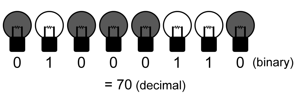
1\. Now, both of you know that exactly one of the light bulbs is faulty, i.e., it is stuck at either on or off. You can know which light bulb is faulty by trying to switch the light bulbs on and off. If your friend knows which light bulb is faulty as well, you can convey a message with 27 = 128 possibilities simply by ignoring the faulty light bulb. However, your friend does not know which light bulb is faulty.
How many different possibilities can you convey? Can you still convey a message with 128 possibilities?
2\. Suppose now both of you know that there are exactly two faulty light bulbs. How many different possibilities can you convey?
* * *
_Bibliographic note: This strategy can be applied to store information in memory cells, where some cells are defective. It has been studied in:_
_A. V. Kuznetsov and B. S. Tsybakov, “Coding in a memory with defective cells,” Probl. Peredachi Inf., vol. 10, no. 2, pp. 52–60, 1974._
_S. I. Gel’fand and M. S. Pinsker, “Coding for channel with random parameters,” Probl. Contr. and Inf. Theory, vol. 9, no. 1, pp. 19–31, 1980._
_C. Heegard and A. El Gamal, “On the capacity of computer memory with defects,” IEEE Trans. Inf. Theory, vol. 29, no. 5, pp. 731-739, 1983._
Apply
-----
Thank you for the nomination and registration. The application deadline has passed.
---
# Unknown
SIAM J. NUMER. ANAL. c ©2018 Society for Industrial and Applied Mathematics Vol. 56, No. 3, pp. 1338–1359 FINITE ELEMENT METHOD AND ITS ANALYSIS FOR A NONLINEAR HELMHOLTZ EQUATION WITH HIGH WAVE NUMBERS ∗ HAIJUN WU † ANDJUN ZOU ‡ Abstract.The well-posedness of a nonlinear Helmholtz equation with an impedance boundary condition is established for high frequencies in two and three dimensions. Stability estimates are derived with explicit dependence on the wave number. Linear finite elements are considered for the discretization of the nonlinear Helmholtz equation, and the well-posedness of the finite element systems is analyzed. Stability and preasymptotic error estimates of the finite element solutions are achieved with explicit dependence on the wave number. Numerical examples are also presented to demonstrate the effectiveness and accuracies of the proposed finite element method for solving the nonlinear Helmholtz equation. Key words.nonlinear Helmholtz equation, high wave number, finite element method, stability, error estimates AMS subject classifications.65N15, 65N12, 65N30, 78A40 DOI.10.1137/17M111314X 1. Introduction.The propagation of electromagnetic waves may be modeled by Maxwell’s equations in physical media with various medium responses. In this work we are interested in high intensity radiation, where the medium quantities may depend on the location, frequency, and magnitude of the propagating field, resulting in a nonlinear electromagnetic wave propagation. We shall consider the time-harmonic propagation in a homogeneous background medium inR d (d= 2,3), where some nonlinear medium, say, the Kerr medium, is sitting inside and occupying a domain Ω 0 . Letω 0 andcbe the angular frequency and the speed of light in vacuum, and letn 0 andn 2 be the index of refraction of the homogeneous medium and the Kerr coefficient of the nonlinear medium, respectively. Then under linear polarization for the electric field, we may come to the following nonlinear Helmholtz (NLH) equation for the electric field after eliminating the magnetic field from the Maxwell system \[8, 9, 12, 22, 23\]: −∆u−k 2 (1 +ε1 Ω 0 |u| 2 )u=finR d ,(1.1) wherek=ω 0 n 0 /cis the wave number,ε(x) = 2n 2 (x)/n 0 represents the Kerr constant satisfying 0< ε�1, and1 Ω 0 is the characteristic function of Ω 0 . There are already many mathematical and numerical studies in the literature for the NLH equation (1.1) under various boundary conditions imposed on the finitely ∗ Received by the editors January 23, 2017; accepted for publication (in revised form) April 12, 2018; published electronically May 15, 2018. http://www.siam.org/journals/sinum/56-3/M111314.html Funding:The work of the first author was partially supported by the NSF of China under grants 11525103, 91630309, and 11621101. The work of the second author was supported by the Hong Kong RGC General Research Fund (project 14306814) and National Natural Science Foun- dation of China/Hong Kong Research Grants Council Joint Research Scheme 2016/17 (project NCUHK437/16). † Department of Mathematics, Nanjing University, Jiangsu 210093, People’s Republic of China (hjw@nju.edu.cn). ‡ Department of Mathematics, Chinese University of Hong Kong, Shatin, N.T., Hong Kong, People’s Republic of China (zou@math.cuhk.edu.hk). 1338 FINITE ELEMENT METHOD FOR A HELMHOLTZ EQUATION1339 truncated subregion of the entire domainR d . A variational framework was developed in \[20\] to prove the existence of nontrivial solutions for the NLH equation ∆u+k 2 u= f, wherefis a nonlinear function that meets five specific conditions, under two special asymptotic decay assumptions on the solution itself and its radial second- order derivative. In addition, the radial symmetric case is also considered, in which infinitely many solutions are shown to exist for different nonlinearities. For the one-dimensional periodic dielectric photonic bandgap structures composed of alternatively arranged nonlinear Kerr material layers, the well-posedness of the NLH equation was established in \[6\], under the two-way boundary conditions that are derived from the standard jump conditions. A numerical scheme was proposed in \[37\] for solving the NLH equation, based on the existence of a stable steady-state solution to a nonlinear Schr ̈odinger type equation and an operator splitting technique. A fourth-order finite difference scheme was proposed in \[22\] for solving (1.1) for the case where the nonlinear medium domain Ω 0 occupies the domain formed by two parallel infinite planes by using a nonlocal two-way artificial boundary condition set on the boundary of Ω 0 . In \[23\], an improved scheme was proposed by introducing some Sommerfeld-type local radiation boundary conditions that are constructed directly in the discrete setting. The high-order scheme was then extended in \[7\] to a three- dimensional setting with cylindrical symmetry under both boundary conditions from \[22, 23\]. In this work we shall carry out a systematical mathematical and numerical study of the NLH system (1.2)–(1.3) in a general setting for both two and three dimensions. We first make a general truncation of the homogeneous mediumR d \\Ω 0 by a finite domain Ω with Ω 0 ⊂Ω. Then we consider the lowest order absorbing boundary condition on the boundary Γ of Ω to arrive at the following NLH system of our interest in this work: −∆u−k 2 (1 +ε1 Ω 0 |u| 2 )u=fin Ω,(1.2) ∂u ∂n +iku=gon Γ,(1.3) wherei= √ −1 denotes the imaginary unit andndenotes the unit outer normal to ∂Ω. One may note thatgdepends on the incident waveu inc , that is,g= ∂u inc ∂n +iku inc . Other kinds of more accurate boundary conditions such as PML may be considered but are much more complicated to analyze both mathematically and numerically and will not be studied in this work. For ease of presentation, we shall assume thatkis constant on Ω and consider only the casek�1 since we are mainly interested in high frequencies in this work, though most of our results are naturally true for low frequencies. The main focus of this work is to study the well-posedness of the NLH system (1.2)–(1.3) and its finite element approximation as well as the error estimates of the finite element solutions for high wave numbers in two and three dimensions. The well-posedness of both the NLH system and its linear finite element approximation is established. Particularly, we emphasize that the stability estimates of the continuous NLH solutions and their finite element solutions are achieved with explicit dependence on the wave number, and the preasymptotic optimal error estimates of the finite element solutions are also derived. To the best of our knowledge, these results and analyses are new, and there are still no similar studies and results available for NLH equations in the literature. We like to point out that the whole analysis in this work is focused on the NLH system (1.2)–(1.3) that is expressed in terms of the total fieldu. But with some 1340HAIJUN WU AND JUN ZOU natural modifications, all our results and analyses can be extended to the case when the NLH system (1.2)–(1.3) is expressed in terms of the scattered fieldu sc :=u−u inc that satisfies −∆u sc −k 2 u sc −k 2 ε1 Ω 0 ( |u sc +u inc | 2 (u sc +u inc )−|u inc | 2 u inc ) = ̃ fin Ω,(1.4) ∂u sc ∂n +iku sc = 0 on Γ,(1.5) where ̃ f:=f+ ∆u inc +k 2 (1 +ε1 Ω 0 |u inc | 2 )u inc . We shall provide further illustrations about this extension in Remarks 2.1 and 3.1. Throughout the paper, we shall use the standard Sobolev spaceH s (Ω), its norm and inner product, and refer to \[10, 15\] for their definitions. But (·,·) and〈·,·〉are used for theL 2 -inner product on the complex-valued spacesL 2 (Ω) andL 2 (Γ), respectively. We will write by‖·‖ s and|·| s the norm and seminorm of the spaceH s (Ω) and by ‖·‖ s,Γ and|·| s,Γ the norm and seminorm ofH s (Γ). In particular, we will often use the weighted energy norm‖|w|‖= (‖∇w‖ 2 0 +k 2 ‖w‖ 2 0 ) 1/2 for anyw∈H 1 (Ω). For the simplicity of notation, we shall frequently useCfor a generic positive constant in most of the subsequent estimates, which is independent of the parameters ε,kand functionsf,gin (1.2)–(1.3), as well as the penalty parameters involved in the subsequent continuous interior penalty FEM. We will also often writeA.Band B&Afor the inequalitiesA≤CBandB≥CA, respectively.AhBis used for an equivalent statement when bothA.BandB.Ahold. We shall consider only the case where the domain Ω is convex, so it is “strictly star-shaped,” which means that there exists a pointx Ω ∈Ω and a positive constantc Ω depending only on Ω such that (x−x Ω )·n≥c Ω ∀x∈∂Ω.(1.6) We shall assume dist(∂Ω,Ω 0 )&diam(Ω 0 ) and frequently use the special function α(x) =x−x Ω ∀x∈ ̄ Ω. We end this section with a detailed plan for the rest of the paper. Section 2 is devoted to the stability estimate of the continuous NLH equation inL 2 -,H 1 -, H 2 -, andL ∞ -norm. We will discuss the piecewise linear continuous finite element approximation of the NLH equation and its error estimates in section 3. To reduce the pollution errors of the linear finite elements, we introduce the continuous interior penalty FEM in section 4. Finally in section 5, we present two numerical examples to demonstrate the effectiveness and accuracies of our proposed finite element method for solving the NLH equation. 2. Stability estimates of the continuous problem.In this section we will establish some stability estimates of the solutions to the continuous NLH equation (1.2)–(1.3), with their bounds depending on the wave number explicitly. We first cite the following two integral identities \[21, Lemma 4.1\], which will play an important role in our subsequent analysis. Lemma2.1.It holds forv∈H 2 (Ω)that d‖v‖ 2 0 + 2Re(v,α·∇v) = ∫ Γ α·n|v| 2 ,(2.1) (d−2)‖∇v‖ 2 0 + 2Re(∇v,∇(α·∇v)) = ∫ Γ α·n|∇v| 2 .(2.2) FINITE ELEMENT METHOD FOR A HELMHOLTZ EQUATION1341 We remark that the identity (2.2) can be viewed as a local version of the Rellich identity for the Laplacian4(cf. \[16\]). 2.1. An auxiliary problem.For the establishment of the well-posedness of the nonlinear system (1.2)–(1.3), we shall use a linearized process to construct a sequence of approximate solutions to linearized Helmholtz equations, show the uniform bounds of these approximate solutions with respect to the wave number, then verify that the limiting solution of this sequence solves our desired NLH system. To do so, we first study the following linear auxiliary problem for a given functionφ∈L ∞ (Ω): −∆u−k 2 (1 +ε1 Ω 0 |φ| 2 )u=fin Ω,(2.3) ∂u ∂n +iku=gon Γ.(2.4) Clearly, the variational formulation of the auxiliary problem reads as (2.5) (∇u,∇v)−k 2 (u,v)−k 2 ε(1 Ω 0 |φ| 2 u,v) +ik〈u,v〉= (f,v) +〈g,v〉 ∀v∈H 1 (Ω). For convenience, we introduce two constants, M(f,g) :=‖f‖ 0 +‖g‖ 0,Γ , ̂ M(f,g) :=M(f,g) +k −1 ‖g‖ 1 2 ,Γ . Then similarly to the stability estimates for the linear Helmholtz equations \[16, 28, 30\], we may derive stability estimates for the auxiliary problem (2.3)–(2.4). Lemma2.2.Ifkε‖φ‖ 2 L ∞ (Ω 0 ) ≤θ 0 for a positive constantθ 0 , then we have ‖|u|‖.M(f,g)and‖u‖ 2 .k ̂ M(f,g).(2.6) Proof.We first takev=uin (2.5), then compute the imaginary and real parts of the resulting equation to obtain k‖u‖ 2 0,Γ = Im((f,u) +〈g,u〉)≤|(f,u)|+ 1 2k ‖g‖ 2 0,Γ + k 2 ‖u‖ 2 0,Γ ,(2.7) ‖∇u‖ 2 0 −k 2 ‖u‖ 2 0 −k 2 ε‖φu‖ 2 0,Ω 0 ≤|(f,u)|+ 1 2k ‖g‖ 2 0,Γ + k 2 ‖u‖ 2 0,Γ ,(2.8) which imply immediately k‖u‖ 2 0,Γ ≤2|(f,u)|+ 1 k ‖g‖ 2 0,Γ ,(2.9) ‖∇u‖ 2 0 −k 2 ‖u‖ 2 0 −k 2 ε‖φu‖ 2 0,Ω 0 ≤2|(f,u)|+ 1 k ‖g‖ 2 0,Γ .(2.10) Then we takev= 2α·∇uin (2.5) and compute the real part of the resulting equation to derive by using Lemma 2.1 that ∫ Γ α·n|∇u| 2 −(d−2)‖∇u‖ 2 0 −k 2 ( ∫ Γ α·n|u| 2 −d‖u‖ 2 0 ) −2k 2 εRe(1 Ω 0 |φ| 2 u,α·∇u)−2kIm〈u,α·∇u〉 = 2 Re ( (f,α·∇u) +〈g,α·∇u〉 ) . Using this relation, (2.9)–(2.10) and (1.6) we can deduce as follows: 1342HAIJUN WU AND JUN ZOU ‖∇u‖ 2 0 +k 2 ‖u‖ 2 0 =− ∫ Γ α·n|∇u| 2 +k 2 ∫ Γ α·n|u| 2 + (d−1) ( ‖∇u‖ 2 0 −k 2 ‖u‖ 2 0 ) + 2k 2 εRe(1 Ω 0 |φ| 2 u,α·∇u) + 2kIm〈u,α·∇u〉+ 2 Re ((f,α·∇u) +〈g,α·∇u〉) ≤−c Ω ‖∇u‖ 2 0,Γ +Ck ( 2|(f,u)|+ 1 k ‖g‖ 2 0,Γ ) + 2k 2 ε ( ‖φu‖ 2 0,Ω 0 + Re(1 Ω 0 |φ| 2 u,α·∇u) ) + c Ω 2 ‖∇u‖ 2 0,Γ + 1 2 ‖∇u‖ 2 0 +C‖f‖ 2 0 +C‖g‖ 2 0,Γ ≤− c Ω 2 ‖∇u‖ 2 0,Γ + 2k 2 ε ( ‖φu‖ 2 0,Ω 0 + ∣ ∣ (1 Ω 0 |φ| 2 u,α·∇u) ∣ ∣ ) + 1 2 ‖∇u‖ 2 0 + k 2 2 ‖u‖ 2 0 +C‖f‖ 2 0 +C‖g‖ 2 0,Γ , which implies ‖|u|‖ 2 ≤4k 2 ε ( ‖φu‖ 2 0,Ω 0 + ∣ ∣ (1 Ω 0 |φ| 2 u,α·∇u) ) +C‖f‖ 2 0 +C‖g‖ 2 0,Γ .(2.11) We can easily see 4k 2 ε ( ‖φu‖ 2 0,Ω 0 + ∣ ∣ (1 Ω 0 |φ| 2 u,α·∇u) ) .k 2 ε‖φ‖ 2 L ∞ (Ω 0 ) ( ‖u‖ 2 0 +‖u‖ 0 ‖∇u‖ 0 ) (2.12) .kε‖φ‖ 2 L ∞ (Ω 0 ) ‖|u|‖ 2 . Clearly we see the existence of a positive constantθ 0 such that the first estimate in (2.6) follows from (2.11) and (2.12) ifkε‖φ‖ 2 L ∞ (Ω 0 ) ≤θ 0 . On the other hand, for the second estimate in (2.6) we may first apply the fol- lowing standard a priori estimate for elliptic equations and (2.3)–(2.4): ‖u‖ 2 .‖∆u‖ 0 +‖u‖ 0 + ∥ ∥ ∥ ∥ ∂u ∂n ∥ ∥ ∥ ∥ 1 2 ,Γ .k 2 ‖u‖ 0 +k 2 ε ∥ ∥ |φ| 2 u ∥ ∥ 0,Ω 0 +‖f‖ 0 +‖g−iku‖ 1 2 ,Γ . Then the desired estimate is a consequence of the first one in (2.6). The followingL ∞ estimate will be crucial to our subsequent analysis. Lemma2.3.Under the same condition of Lemma2.2, it holds that ‖u‖ L ∞ (Ω 0 ) .k d−3 2 M(f,g).(2.13) Proof.LetG(x−y) be the Green’s function of the linear Helmholtz equation −∆u−k 2 u=fwith the standard radiation condition. Letr=|x−y|; then we know G(x−y) = i 4 H (1) 0 (kr) ford= 2, e ikr 4πr ford= 3. Some simple calculations show that the solutionuto (2.3)–(2.4) meets the following integral representation: u(x) = ∫ Ω G(x−y) ( f(y) +k 2 ε1 Ω 0 |φ(y)| 2 u(y) ) dy(2.14) + ∫ Γ (g−iku)G(x−y)ds y − ∫ Γ u(y) ∂G(x−y) ∂n y ds y . FINITE ELEMENT METHOD FOR A HELMHOLTZ EQUATION1343 Clearly, |G(x−y)|. 1 r ifd= 3.(2.15) Ford= 2, we know from \[35, p. 211\] that |G(x−y)|. 1 √ kr ifd= 2.(2.16) Then by using a standard technique to remove a small ball centered atxwe derive ∫ Ω |G(x−y)| 2 dy.k d−3 .(2.17) On the other hand, we know ∇ y G(x−y) = − ik 4 H (1) 1 (kr) y−x r ford= 2, e ikr 4πr ( ik−r −1 ) y−x r ford= 3. Supposex∈Ω 0 . Since dist(∂Ω,Ω 0 )&diam(Ω 0 ), we have for anyy∈Γ |G(x−y)|.k d−3 2 and|∇ y G(x−y)|.k d−1 2 . Then it follows from these estimates, (2.14), and (2.17) that |u(x)|.k d−3 2 ( ‖f‖ 0 +k 2 ε‖φ‖ 2 L ∞ (Ω 0 ) ‖u‖ 0 +‖g‖ 0,Γ +k‖u‖ 0,Γ ) .k d−3 2 M(f,g), where we have used Lemma 2.2, (2.9), and the assumption thatkε‖φ‖ 2 L ∞ (Ω 0 ) ≤θ 0 to derive the last inequality. This completes the proof of the desired estimate (2.13). 2.2. Existence and stability estimates of the NLH solutions.We consider an iterative procedure to establish the existence and stability of the solutions to the NLH system (1.2)–(1.3). Findu l ∈H 1 (Ω) forl= 1,2,...by solving the linearized Helmholtz equation: −∆u l −k 2 ( 1 +ε1 Ω 0 ∣ ∣ u l−1 ∣ ∣ 2 ) u l =fin Ω,(2.18) ∂u l ∂n +iku l =gon Γ.(2.19) We first derive the following stability estimates of the sequence{u l }. Lemma2.4.There exists a positive constantθ 1 such that the following estimates hold forl= 1,2,...ifkε ∥ ∥ u 0 ∥ ∥ 2 L ∞ (Ω 0 ) ≤k d−2 εM(f,g) 2 ≤θ 1 : ∥ ∥ ∣ ∣ u l ∣ ∣ ∥ ∥ 0 .M(f,g), ∥ ∥ u l ∥ ∥ 2 .k ̂ M(f,g), ∥ ∥ u l ∥ ∥ L ∞ (Ω 0 ) .k d−3 2 M(f,g).(2.20) Proof.Ifkε ∥ ∥ u l−1 ∥ ∥ 2 L ∞ (Ω 0 ) ≤θ 0 , then Lemma 2.2 implies the estimates in (2.20). Thereforekε ∥ ∥ u l ∥ ∥ 2 L ∞ (Ω 0 ) ≤θ 0 ifk d−2 εM(f,g) 2 is small enough. Then the proof of the lemma follows by the induction. 1344HAIJUN WU AND JUN ZOU Next we prove the well-posedness of the NLH problem (1.2)–(1.3) under certain conditions by showing the convergence of the sequence{u l }. Theorem2.5.There exists a constantθ 2 >0such that ifk d−2 εM(f,g) 2 ≤θ 2 , then the NLH system(1.2)–(1.3)attains a unique solutionusatisfying the estimates ‖∇u‖ 0 +k‖u‖ 0 .M(f,g),‖u‖ 2 .k ̂ M(f,g),‖u‖ L ∞ (Ω 0 ) .k d−3 2 M(f,g).(2.21) Proof.Let the sequenceu l forl≥1 be defined by (2.18) and (2.19). Then it is easy to check that the differencev l =u l+1 −u l satisfies −∆v l −k 2 ( 1 +ε1 Ω 0 ∣ ∣ u l ∣ ∣ 2 ) v l =k 2 ε1 Ω 0 u l ( ∣ ∣ u l ∣ ∣ 2 − ∣ ∣ u l−1 ∣ ∣ 2 ) in Ω, ∂v l ∂n +ikv l = 0 on Γ. Now we suppose that the conditions of Lemma 2.4 are satisfied; then it follows from Lemmas 2.2 and 2.4 that ∥ ∥ ∣ ∣ v l ∣ ∣ ∥ ∥ ≤Ck 2 ε ∥ ∥ ∥ u l ( ∣ ∣ u l ∣ ∣ 2 − ∣ ∣ u l−1 ∣ ∣ 2 ) ∥ ∥ ∥ 0,Ω 0 ≤Ck 2 ε ∥ ∥ u l ∥ ∥ L ∞ (Ω 0 ) ( ∥ ∥ u l ∥ ∥ L ∞ (Ω 0 ) + ∥ ∥ u l−1 ∥ ∥ L ∞ (Ω 0 ) ) ∥ ∥ v l−1 ∥ ∥ 0,Ω 0 ≤Ck 2 ε ( k d−3 2 M(f,g) ) 2 ∥ ∥ v l−1 ∥ ∥ 0 ≤Ck d−2 εM(f,g) 2 ∥ ∥ ∣ ∣ v l−1 ∣ ∣ ∥ ∥ . Clearly there exists a constant ̃ θ 2 satisfying 0< ̃ θ 2 < θ 1 (withθ 1 from Lemma 2.4) such that ifk d−2 εM(f,g) 2 ≤ ̃ θ 2 we have ∥ ∥ ∣ ∣ v l ∣ ∣ ∥ ∥ ≤ 1 2 ∥ ∥ ∣ ∣ v l−1 ∣ ∣ ∥ ∥ , which implies that‖|v l |‖ ≤2 −l ‖|v 0 |‖. Hence{u l }is a Cauchy sequence with respect to the energy norm. Moreover, we have ∥ ∥ v l ∥ ∥ 2 .k 3 ε ∥ ∥ ∥ u l ( ∣ ∣ u l ∣ ∣ 2 − ∣ ∣ u l−1 ∣ ∣ 2 ) ∥ ∥ ∥ 0,Ω 0 .k d−1 εM(f,g) 2 ∥ ∥ ∣ ∣ v l−1 ∣ ∣ ∥ ∥ .k ∥ ∥ ∣ ∣ v l−1 ∣ ∣ ∥ ∥ , which shows that{u l }is also a Cauchy sequence in theH 2 -norm. As a consequence, u:= lim l→∞ u l satisfies the NLH equation (1.2)–(1.3) and the stability estimates in (2.21). It remains to prove the uniqueness. Supposewis another solution to (1.2)–(1.3) satisfying the estimates in (2.21). Letv=u−w; then we can easily see −∆v−k 2 (1 +ε1 Ω 0 |u| 2 )v=k 2 εw ( |u| 2 −1 Ω 0 |w| 2 ) in Ω, ∂v ∂n +ikv= 0 on Γ. Applying Lemma 2.2, we have ‖|v|‖≤Ck 2 ε ∥ ∥ w ( |u| 2 −|w| 2 ) ∥ ∥ 0,Ω 0 ≤Ck d−2 εM(f,g) 2 ‖|v|‖. Then it is easy to see that there exists a constantθ 2 satisfying 0< θ 2 < ̃ θ 2 such that ‖|v|‖ ≤ 1 2 ‖|v|‖ifk d−2 εM(f,g) 2 ≤θ 2 . This implies the uniqueness of the solutions to the NLH system (1.2)–(1.3) and so completes the proof of the theorem. FINITE ELEMENT METHOD FOR A HELMHOLTZ EQUATION1345 Remark2.1. If we consider the NLH system (1.4)–(1.5) in terms of the scattered fieldu sc :=u−u inc , instead of the NLH system (1.2)–(1.3) in terms of the total field u, then the iterative scheme (2.18)–(2.19) is equivalent to the following one: −∆u l sc −k 2 u l sc −k 2 ε1 Ω 0 ( ∣ ∣ u l−1 sc +u inc ∣ ∣ 2 (u l sc +u inc )−|u inc | 2 u inc ) = ̃ fin Ω,(2.22) ∂u l sc ∂n +iku l sc = 0 on Γ,(2.23) where ̃ f:=f+ ∆u inc +k 2 (1 +ε1 Ω 0 |u inc | 2 )u inc . By following our previous analysis for (2.18)–(2.19), one may show that the sequence u l sc converges if‖|u 0 sc |‖.‖ ̃ f‖ 0 , ∥ ∥ u 0 sc ∥ ∥ L ∞ (Ω 0 ) ≤k d−3 2 ‖ ̃ f‖ 0 ,and max ( k d−2 ε‖ ̃ f‖ 2 0 , kε‖u inc ‖ 2 L ∞ (Ω 0 ) ) ≤θ(2.24) for some constantθsufficiently small. And as a consequence, the following estimates hold under the above conditions: k‖u sc ‖ 0 +‖∇u sc ‖ 0 +k −1 ‖u sc ‖ 2 +k 3−d 2 ‖u sc ‖ L ∞ (Ω 0 ) .‖ ̃ f‖ 0 .(2.25) We omit the details. 3. Finite element methods and error estimates.We now discuss the finite element approximation of the NLH system (1.2)–(1.3). LetT h be a quasi-uniform family of triangulations of sizehwith simplicial elements over the domain Ω. For any elementK∈ T h , we defineh K := diam(K) andh= max K∈T h h K . LetV h be the continuous piecewise linear finite element space associated with the triangulationT h : V h := { v h ∈H 1 (Ω) :v h | K ∈P 1 (K)∀K∈T h } , whereP 1 (K) denotes the set of all linear polynomials onK. Now we propose to approximate the solution to the NLH system (1.2)–(1.3) by the finite element solutionu h ∈V h that solves the following equation for anyv h ∈V h : (∇u h ,∇v h )−k 2 ( (1 +ε1 Ω 0 |u h | 2 )u h ,v h ) +ik〈u h ,v h 〉= (f,v h ) +〈g,v h 〉.(3.1) For our subsequent analysis, we need an elliptic projectionP h :H 1 (Ω)7→V h defined by (∇v h ,∇P h w) +ik〈v h ,P h w〉= (∇v h ,∇w) +ik〈v h ,w〉 ∀v h ∈V h .(3.2) The standard finite element error estimates for elliptic problems give the optimal approximation accuracies of the projectionP h inH 1 - andL 2 -norm (see \[36, 10, 39\]): ‖w−P h w‖ 0 .h‖|w−P h w|‖.h 2 |w| 2 .(3.3) 3.1. Discrete Nirenberg inequality.In this subsection, we derive a very im- portant discrete version of the following Nirenberg inequality \[33\] for our subsequent analysis: ‖u‖ L ∞ .‖u‖ 1− d 4 0 |u| d 4 2 +‖u‖ 0 .(3.4) 1346HAIJUN WU AND JUN ZOU For this purpose, we first introduce the discrete Laplacian operatorA h :V h 7→V h : (A h v h ,w h ) = (∇v h ,∇w h ) +ik〈v h ,w h 〉 ∀w h ∈V h .(3.5) Note thatA h can be viewed as a discrete version of the Laplacian operator−∆ under the impedance boundary condition ∂u ∂n +iku= 0 on Γ and‖A h v h ‖ 0 as a discrete H 2 -norm of anyv h ∈V h . Now we can establish a discrete Nirenberg inequality that plays a crucial role in the analysis of the finite element solutions in (3.1) to the NLH system (1.2)–(1.3). Lemma3.1.It holds forkh.1that ‖v h ‖ L ∞ .‖v h ‖ 1− d 4 0 ‖A h v h ‖ d 4 0 +‖v h ‖ 0 ∀v h ∈V h .(3.6) Proof.For anyv h ∈V h , letvbe the solution to the elliptic problem: −∆v=A h v h in Ω; ∂v ∂n +ikv= 0 on Γ.(3.7) Clearly, we see thatv∈H 1 (Ω) satisfies (∇v,∇w h ) +ik〈v,w h 〉= (A h v h ,w h ) = (∇v h ,∇w h ) +ik〈v h ,w h 〉 ∀w h ∈V h , which indicates thatv h is the finite element approximation to the elliptic problem (3.7). Using the regularity and finite element theory for elliptic PDEs we knowv∈ H 2 (Ω) and‖v‖ 2 .‖A h v h ‖ 0 and the error estimates h‖v−v h ‖ 1 +‖v−v h ‖ 0 .h 2 |v| 2 .h 2 ‖A h v h ‖,(3.8) whose proof is omitted (by using the fact thatv h = P h v). LetI h vbe the finite element interpolant ofv. It follows from the inverse inequality and the interpolation error estimate that ‖v h ‖ L ∞ ≤‖v h −I h v‖ L ∞ +‖I h v‖ L ∞ .h − d 2 ‖v h −I h v‖ 0 +‖v‖ L ∞ .h 2− d 2 ‖A h v h ‖ 0 +‖v‖ L ∞ . From (3.4), ‖v h ‖ L ∞ .h 2− d 2 ‖A h v h ‖ 0 +‖v‖ 1− d 4 0 ‖A h v h ‖ d 4 0 +‖v‖ 0 .(3.9) By takingw h =A h v h in (3.5) and using the inverse inequality we have ‖A h v h ‖ 2 0 = (∇v h ,∇A h v h ) +ik〈v h ,A h v h 〉. ( h −2 +kh −1 ) ‖v h ‖ 0 ‖A h v h ‖ 0 , which implies forkh.1 that ‖A h v h ‖ 0 .h −2 ‖v h ‖ 0 . Then using this estimate and (3.8), we can get ‖v‖ 0 ≤‖v h ‖ 0 +‖v−v h ‖ 0 .‖v h ‖ 0 +h 2 ‖A h v h ‖ 0 .‖v h ‖ 0 , h 2− d 2 ‖A h v h ‖ 0 = ( h 2 ‖A h v h ‖ 0 ) 1− d 4 ‖A h v h ‖ d 4 0 .‖v h ‖ 1− d 4 0 ‖A h v h ‖ d 4 0 . Now the discrete Nirenberg inequality (3.6) follows by combining these two estimates and (3.9). This completes the proof of the lemma. FINITE ELEMENT METHOD FOR A HELMHOLTZ EQUATION1347 3.2. A discrete auxiliary problem.We shall follow our analyses of the con- tinuous NLH system (1.2)–(1.3) to study its finite element solutions in (3.1). So for a given functionφ∈L ∞ (Ω), we introduce the finite element approximation to the auxiliary problem (2.5). Findu h ∈V h that solves the equation for anyv h ∈V h : (∇u h ,∇v h )−k 2 (( 1 +ε1 Ω 0 |φ| 2 ) u h ,v h ) +ik〈u h ,v h 〉= (f,v h ) +〈g,v h 〉.(3.10) LetM(f,g) andθ 0 be two constants introduced in Lemma 2.2; then we can establish the stability of the finite element problem (3.10). Lemma3.2.Ifkε‖φ‖ 2 L ∞ (Ω 0 ) ≤θ 0 , there exists a constantC 0 >0such that the finite element solutionsu h to the approximation system(3.10)are stable fork 3 h 2 ≤ C 0 : ‖|u h |‖.M(f,g).(3.11) Proof.Just like the analysis we did for the continuous problem in subsection 2.1, we first takev h =u h in (3.10) to obtain k‖u h ‖ 2 0,Γ ≤2|(f,u h )|+ 1 k ‖g‖ 2 0,Γ ,(3.12) ‖∇u h ‖ 2 0 −k 2 ‖u h ‖ 2 0 −k 2 ε‖φu h ‖ 2 0,Ω 0 ≤2|(f,u h )|+ 1 k ‖g‖ 2 0,Γ .(3.13) But the second test function we took in the analysis for the continuous case can not be copied now due to the fact thatα·∇u h 6∈V h . We circumvent this difficulty by a duality argument. Letw∈H 2 (Ω) be the solution of the following problem: −∆w−k 2 ( 1 +ε1 Ω 0 |φ| 2 ) w=u h in Ω,(3.14) ∂w ∂n −ikw= 0 on Γ.(3.15) Since the conjugate ofwis the solution to (2.3)–(2.4) withf= u h andg= 0, the following regularity estimate holds under the conditions of Lemma 2.2: ‖|w|‖.‖u h ‖ 0 and‖w‖ 2 .k‖u h ‖ 0 .(3.16) Now we multiply (3.14) byu h and then apply (3.2) and (3.10) to obtain ‖u h ‖ 2 0 = (∇u h ,∇w)−k 2 (( 1 +ε1 Ω 0 |φ| 2 ) u h ,w ) +ik〈u h ,w〉 = (∇u h ,∇P h w) +ik〈u h ,P h w〉−k 2 (( 1 +ε1 Ω 0 |φ| 2 ) u h ,w ) = (f,w) +〈g,w〉+ (f,P h w−w) +〈g,P h w−w〉 −k 2 (u h ,w−P h w)−k 2 ε ( 1 Ω 0 |φ| 2 u h ,w−P h w ) . Using the solutionuto the auxiliary problem (2.3)–(2.4), we know from (2.5) and (3.14)–(3.15) that (f,w) +〈g,w〉= (u,u h ). Then we can further derive from (3.3), Lemma 2.2, and (3.16) that ‖u h ‖ 2 0 .|(u,u h )|+‖f‖ 0 ‖w−P h w‖ 0 +‖g‖ 0,Γ ‖w−P h w‖ 0,Γ +k 2 ‖u h ‖ 0 ‖w−P h w‖ 0 +kθ 0 ‖u h ‖ 0 ‖w−P h w‖ 0 .k −1 M(f,g) ( ‖u h ‖ 0 +kh 3 2 |w| 2 ) + ( k 2 h 2 +kθ 0 h 2 ) ‖u h ‖ 0 |w| 2 .k −1 M(f,g) ( 1 +k 2 h 3 2 ) ‖u h ‖ 0 + ( k 3 h 2 +θ 0 k 2 h 2 ) ‖u h ‖ 2 0 , 1348HAIJUN WU AND JUN ZOU and after canceling the common factor‖u h ‖ 0 , we come to ‖u h ‖ 0 .k −1 M(f,g) + ( k 3 h 2 +θ 0 k 2 h 2 ) ‖u h ‖ 0 . This indicates the existence of a constantC 0 >0 such that ‖u h ‖ 0 .k −1 M(f,g)(3.17) ifk 3 h 2 ≤C 0 . Next we estimate‖∇u h ‖ 0 . It follows from (3.13) that ‖∇u h ‖ 2 0 ≤k 2 ‖u h ‖ 2 0 +k 2 ε‖φu h ‖ 2 0,Ω 0 + 2|(f,u h )|+ 1 k ‖g‖ 2 0,Γ (3.18) .k 2 ‖u h ‖ 2 0 +k 2 ε‖φ‖ 2 L ∞ (Ω 0 ) ‖u h ‖ 2 0 + 1 k 2 ‖f‖ 2 0 + 1 k ‖g‖ 2 0,Γ .M(f,g) 2 . This, along with (3.17), yields the desired estimate (3.11). The next lemma provides the estimates of the error between the solution to the continuous problem (2.5) and its finite element solution to the discretization (3.10), whereθ 0 andC 0 are two constants introduced in Lemmas 2.2 and 3.2, respectively. Lemma3.3.Letuandu h be the solutions to(2.5)and(3.10), respectively. Then the error estimates hold under the conditions thatkε‖φ‖ 2 L ∞ (Ω 0 ) ≤θ 0 andk 3 h 2 ≤C 0 : ‖|u−u h |‖.(kh+k 3 h 2 ) ̂ M(f,g)and‖u−u h ‖ 0 .k 2 h 2 ̂ M(f,g).(3.19) Proof.Let ̃u h = P h ube the elliptic projection ofu; then it follows readily from the definition (3.2) ofP h that (∇ ̃u h ,∇v h ) +ik〈 ̃u h ,v h 〉= (∇u,∇v h ) +ik〈u,v h 〉 ∀v h ∈V h ,(3.20) which, along with (3.3) and Lemma 2.2, implies ‖u− ̃u h ‖ 0 +h‖|u− ̃u h |‖.kh 2 ̂ M(f,g).(3.21) It remains to estimateη h :=u h − ̃u h . For anyv h ∈V h , we can see thatη h solves (∇η h ,∇v h )−k 2 (( 1 +ε1 Ω 0 |φ| 2 ) η h ,v h ) +ik〈η h ,v h 〉(3.22) = (f,v h ) +〈g,v h 〉−(∇u,v h )−ik〈u,v h 〉+k 2 (( 1 +ε1 Ω 0 |φ| 2 ) ̃u h ,v h ) =k 2 (( 1 +ε1 Ω 0 |φ| 2 ) ( ̃u h −u),v h ) . Applying the stability estimate of Lemma 3.2 to this problem leads to ‖|η h |‖.k 2 ∥ ∥ ( 1 +ε1 Ω 0 |φ| 2 ) ( ̃u h −u) ∥ ∥ 0 .k 2 ∥ ∥ ̃u h −u ∥ ∥ 0 .k 3 h 2 ̂ M(f,g). This, combining (3.21), gives the desired estimate (3.19) by the triangle inequality. We end this subsection with anL ∞ estimate of the finite element solutionu h to the approximation (3.10), and this estimate is also essential to our subsequent analysis. Lemma3.4.Under the same conditions as in Lemma3.3, the followingL ∞ esti- mate holds for the finite element solutionu h to the system(3.10): ‖u h ‖ L ∞ (Ω 0 ) .|lnh|k d−3 2 ̂ M(f,g). FINITE ELEMENT METHOD FOR A HELMHOLTZ EQUATION1349 Proof.As in the proof of Lemma 3.3, we let ̃u h = P h uandη h =u h − ̃u h . Then we have by the triangle inequality that ‖u h ‖ L ∞ (Ω 0 ) ≤‖η h ‖ L ∞ (Ω 0 ) +‖ ̃u h −u‖ L ∞ (Ω 0 ) +‖u‖ L ∞ (Ω 0 ) .(3.23) Then it remains to estimate the first two terms on the right-hand side. It follows first from the interior maximum-norm estimates for finite element solutions \[34, Theorem 5.1\], Lemma 2.3, (3.3), and Lemma 2.2 that ‖u− ̃u h ‖ L ∞ (Ω 0 ) .|lnh|‖u‖ L ∞ (Ω) +‖u− ̃u h ‖ 0 .|lnh|‖u‖ L ∞ (Ω) +h‖|u|‖(3.24) . ( |lnh|k d−3 2 +h ) M(f,g).|lnh|k d−3 2 M(f,g), where we have usedk 3 h 2 ≤C 0 to derive the last inequality. Now we estimate‖η h ‖ L ∞ . From the definition (3.5) ofA h and (3.22), we have (A h η h ,v h ) =k 2 (( 1 +ε1 Ω 0 |φ| 2 ) (u h −u),v h ) ∀v h ∈V h . Clearly, we can derive from (3.19) and (3.21) that ‖η h ‖ 0 .‖u h −u‖ 0 +‖u− ̃u h ‖ 0 .k 2 h 2 ̂ M(f,g),(3.25) ‖A h η h ‖ 0 .k 2 ∥ ∥ ( 1 +ε1 Ω 0 |φ| 2 ) (u h −u) ∥ ∥ 0 .k 4 h 2 ̂ M(f,g).(3.26) Now we defineη∈H 1 (Ω) by the variational equation: (∇η,∇v) +ik〈η,v〉=k 2 (( 1 +ε1 Ω 0 |φ| 2 ) (u h −u),v ) ∀v∈H 1 (Ω).(3.27) Using the regularity estimate of the elliptic PDEs, we have ‖η‖ 2 .k 2 ∥ ∥ ( 1 +ε1 Ω 0 |φ| 2 ) (u h −u) ∥ ∥ 0 .k 4 h 2 ̂ M(f,g).(3.28) To go further, we can easily verify that (∇η h ,∇v) +ik〈η h ,v〉= (∇η,∇v) +ik〈η,v〉.(3.29) Soη h can be viewed as the finite element approximation ofη, and it then follows from the standard arguments for the C ́ea lemma and the interpolation error estimates that ‖η−η h ‖ 0 .h 2 |η| 2 .k 4 h 4 ̂ M(f,g).(3.30) Now we take a subdomain Ω 1 in Ω such that Ω 0 ⊂Ω 1 and dist(∂Ω 0 ,∂Ω 1 )hdist(∂Ω 1 ,∂Ω)h1; then we get from (3.29) and the interior maximum-norm estimates \[34, Theorem 5.1\] ‖η−η h ‖ L ∞ (Ω 0 ) .|lnh|‖η−I h η‖ L ∞ (Ω 1 ) +‖η−η h ‖ 0 .|lnh|h 2 |η| W 2,∞ (Ω 1 ) +k 4 h 4 ̂ M(f,g). From (3.27), the Schauder interior estimates for the elliptic equations \[24\], and the Nirenberg and discrete Nirenberg inequalities (3.4) and (3.6), we conclude that ‖η‖ W 2,∞ (Ω 1 ) .‖η‖ L ∞ (Ω) +k 2 ‖η h ‖ L ∞ (Ω) +k 2 ‖ ̃u h −u‖ L ∞ (Ω) .‖η‖ L ∞ (Ω) +k 2 ‖η h ‖ L ∞ (Ω) +k 2 ‖ ̃u h −I h u‖ L ∞ (Ω) +k 2 ‖u‖ L ∞ (Ω) .‖η‖ 2 +k 2 ‖η h ‖ 1− d 4 0 ‖A h η h ‖ d 4 0 +k 2 ‖ ̃u h −I h u‖ 1− d 4 0 ‖A h ( ̃u h −I h u)‖ d 4 0 +k 2 ‖u‖ 1− d 4 0 ‖u‖ d 4 2 .k 2 k d 2 +2 h 2 ̂ M(f,g) +k d 2 +1 ̂ M(f,g), 1350HAIJUN WU AND JUN ZOU where we have used (3.28), (3.25)–(3.26), and Lemma 2.2 to derive the last inequality. By combining the above two estimates and usingk 3 h 2 ≤C 0 , we have ‖η−η h ‖ L ∞ (Ω 0 ) .|lnh| ( k d 2 +4 h 4 +k d 2 +1 h 2 ) ̂ M(f,g) +k 4 h 4 ̂ M(f,g) =|lnh|h 1 3 ( k 11 2 h 11 3 +k 5 2 h 5 3 ) k d−3 2 ̂ M(f,g) +k 4 h 4 ̂ M(f,g) .k d−3 2 ̂ M(f,g).(3.31) On the other hand, by rewriting (3.27) we can see thatη∈H 1 (Ω) solves the equation (∇η,∇v) +ik〈η,v〉−k 2 (η,v) =k 2 (η h −η,v) +k 2 ( ̃u h −u,v ) +k 2 ( ε1 Ω 0 |φ| 2 (u h −u),v ) ∀v∈H 1 (Ω), so we can apply Lemma 2.3 to obtain ‖η‖ L ∞ (Ω 0 ) .k d−3 2 k 2 ( ‖η h −η‖ 0 +‖ ̃u h −u‖ 0 +k −1 ‖u h −u‖ 0 ) .k d−3 2 k 2 ( k 4 h 4 +kh 2 ) ̂ M(f,g) = ( k 6 h 4 +k 3 h 2 ) k d−3 2 ̂ M(f,g).k d−3 2 ̂ M(f,g). Combining this and (3.31) gives ‖η h ‖ L ∞ (Ω 0 ) .k d−3 2 ̂ M(f,g).(3.32) Then the desiredL ∞ estimate follows readily from (2.13), (3.23)–(3.24), and (3.32). 3.3. Existence of the finite element solution.Following the analysis for the continuous NLH equation in section 2.2, we consider an iterative procedure to establish the existence and stability of the finite element solutions to the discrete NLH system (3.1): for a givenu 0 h ∈V h , findu l h ∈V h forl= 1,2,...such that ( ∇u l h ,∇v h ) −k 2 (( 1+ε1 Ω 0 ∣ ∣ u l−1 h ∣ ∣ 2 ) u l h ,v h ) +ik 〈 u l h ,v h 〉 =(f,v h ) +〈g,v h 〉 ∀v h ∈V h . (3.33) The following lemma gives the stability estimates of this sequenceu l h forl≥1. Lemma3.5.There exists a constantθ 3 >0such that ifkε ∥ ∥ u 0 h ∥ ∥ 2 L ∞ (Ω 0 ) ≤ |lnh| 2 k d−2 ε ̂ M(f,g) 2 ≤θ 3 andk 3 h 2 ≤C 0 (from Lemma3.2), then the following stability estimates hold forl= 1,2,...: ∥ ∥ ∣ ∣ u l h ∣ ∣ ∥ ∥ .M(f,g)and ∥ ∥ u l h ∥ ∥ L ∞ (Ω 0 ) .|lnh|k d−3 2 ̂ M(f,g).(3.34) Proof.First we can easily see that ifkε ∥ ∥ u l−1 h ∥ ∥ 2 L ∞ (Ω 0 ) ≤θ 0 , then (3.34) follows di- rectly from Lemmas 3.2 and 3.4. This implies immediately the existence of a constant θ 3 >0 such that kε ∥ ∥ u l h ∥ ∥ 2 L ∞ (Ω 0 ) ≤C|lnh| 2 k d−2 ε ̂ M(f,g) 2 ≤θ 0 if|lnh| 2 k d−2 ε ̂ M(f,g) 2 ≤θ 3 . Now the proof of the lemma follows by induction. FINITE ELEMENT METHOD FOR A HELMHOLTZ EQUATION1351 We are now ready to show the convergence of the sequence{u l h }to a finite element solution of the discrete NLH system (3.1) under proper conditions. Theorem3.6.There exists a constant ̃ C >0such that ifk 3 h 2 ≤C 0 (from Lemma3.2) andσ:= ̃ C|lnh| 2 k d−2 ε ̂ M(f,g) 2 <1, then the finite element system (3.1)attains a unique solutionu h satisfying the stability estimates: ‖∇u h ‖ 0 +k‖u h ‖ 0 .M(f,g)and‖u h ‖ L ∞ (Ω 0 ) .|lnh|k d−3 2 ̂ M(f,g).(3.35) Moreover, if‖|u 0 h |‖≤M(f,g)and ∥ ∥ u 0 h ∥ ∥ L ∞ (Ω 0 ) ≤|lnh|k d−3 2 ̂ M(f,g), then the iterative scheme(3.33)converges at a rate given by ∥ ∥ ∣ ∣ u l h −u h ∣ ∣ ∥ ∥ .σ l M(f,g).(3.36) Proof.It is easy to verify using the iterative scheme (3.33) that the difference v l h :=u l+1 h −u l h solves the following equation: (∇v l h ,∇v h )−k 2 (( 1 +ε1 Ω 0 ∣ ∣ u l h ∣ ∣ 2 ) v l h ,v h ) +ik 〈 v l h ,v h 〉 =k 2 ε ( 1 Ω 0 u l h ( ∣ ∣ u l h ∣ ∣ 2 − ∣ ∣ u l−1 h ∣ ∣ 2 ) ,v h ) ∀v h ∈V h . Under the conditions of Lemma 3.5, we havekε ∥ ∥ u l h ∥ ∥ 2 L ∞ (Ω 0 ) ≤θ 0 . Then we conclude from Lemmas 3.2 and 3.5 that ∥ ∥ ∣ ∣ v l h ∣ ∣ ∥ ∥ .k 2 ε ∥ ∥ ∥ u l h ( ∣ ∣ u l h ∣ ∣ 2 − ∣ ∣ u l−1 h ∣ ∣ 2 ) ∥ ∥ ∥ 0,Ω 0 .kε ∥ ∥ u l h ∥ ∥ L ∞ (Ω 0 ) ( ∥ ∥ u l h ∥ ∥ L ∞ (Ω 0 ) + ∥ ∥ u l−1 h ∥ ∥ L ∞ (Ω 0 ) ) ∥ ∥ ∣ ∣ v l−1 h ∣ ∣ ∥ ∥ .|lnh| 2 k d−2 ε ̂ M(f,g) 2 ∥ ∥ ∣ ∣ v l−1 h ∣ ∣ ∥ ∥ . That is,‖|v l h |‖ ≤ ̃ C|lnh| 2 k d−2 ε ̂ M(f,g) 2 ‖|v l−1 h |‖for some constant ̃ C >0. Therefore { u l h } is a Cauchy sequence ifσ= ̃ C|lnh| 2 k d−2 ε ̂ M(f,g) 2 <1 and converges, say, to u h . It is easy to check from (3.33) thatu h solves (3.1), and the estimates (3.35) are a consequence of (3.34). The uniqueness of the solutionsu h to (3.1) can be proved in a similar manner to the one for Theorem 2.5, and the details are omitted. To see the error estimate (3.36), we recall the previous estimate‖|v l h |‖≤σ‖|v l−1 h |‖. Then we readily obtain‖|v l h |‖ ≤σ l ‖|v 0 h |‖.σ l M(f,g) and‖|u l h −u h |‖.σ l /(1− σ)M(f,g). This completes the proof of the theorem. 3.4. Error estimates of finite element solutions.In this subsection we esti- mate the error between the continuous solutionuto the NLH system (1.2)–(1.3) and its finite element solutionu h to the discrete NLH system (3.1). Theorem3.7.There exist constantsC 0 ,C 1 ,C 2 ,θ >0such that ifk 3 h 2 ≤C 0 and |lnh| 2 k d−2 ε ̂ M(f,g) 2 ≤θ; then the following error estimate between the finite element solutionu h to(3.1)and the NLH solutionuto(1.2)–(1.3)holds: ‖|u−u h |‖≤(C 1 kh+C 2 k 3 h 2 ) ̂ M(f,g).(3.37) Proof.We know from Theorems 2.5 and 3.6 thatuandu h are the limits of two sequences{u l }and{u l h }defined by the systems (2.18)–(2.19) and (3.33), respectively. So it is natural to estimate the erroru l −u l h . 1352HAIJUN WU AND JUN ZOU We know from (2.18)–(2.19) thatu l solves the variational formulation forl= 1,2,...andv∈H 1 (Ω): (∇u l ,∇v)−k 2 (( 1 +ε1 Ω 0 ∣ ∣ u l−1 ∣ ∣ 2 ) u l ,v ) +ik 〈 u l ,v 〉 = (f,v) +〈g,v〉.(3.38) We now define ̃u 0 h =u 0 h and ̃u l h ∈V h forl= 1,2,...to be the solution to the following problem for allv h ∈V h : (∇ ̃u l h ,∇v h )−k 2 (( 1 +ε1 Ω 0 ∣ ∣ u l−1 ∣ ∣ 2 ) ̃u l h ,v h ) +ik 〈 ̃u l h ,v h 〉 = (f,v h ) +〈g,v h 〉.(3.39) Clearly we can apply Lemma 3.3 withφ=u l−1 to the system (3.38) and its finite element approximation (3.39) to get forl≥1 ∥ ∥ ∣ ∣ u l − ̃u l h ∣ ∣ ∥ ∥ .(kh+k 3 h 2 ) ̂ M(f,g).(3.40) Usingu l −u l h = (u l − ̃u l h ) + ( ̃u l h −u l h ), we still need to estimateη l h := ̃u l h −u l h . We know from (3.33) and (3.39) thatη l h ∈V h solves (∇η l h ,∇v h )−k 2 (( 1 +ε1 Ω 0 ∣ ∣ u l−1 ∣ ∣ 2 ) η l h ,v h ) +ik 〈 η l h ,v h 〉 (3.41) =k 2 ε ( 1 Ω 0 ( ∣ ∣ u l−1 ∣ ∣ 2 − ∣ ∣ u l−1 h ∣ ∣ 2 ) u l h ,v h ) ∀v h ∈V h . Then we can apply the stability estimate in Lemmas 3.2, 2.4, and 3.5 to obtain ∥ ∥ ∣ ∣ η l h ∣ ∣ ∥ ∥ .k 2 ε ∥ ∥ ( ∣ ∣ u l−1 ∣ ∣ 2 − ∣ ∣ u l−1 h ∣ ∣ 2 ) u l h ∥ ∥ 0,Ω 0 .k 2 ε ( |lnh|k d−3 2 ̂ M(f,g) ) 2 ∥ ∥ u l−1 −u l−1 h ∥ ∥ 0 .|lnh| 2 k d−2 ε ̂ M(f,g) 2 ( ∥ ∥ ∣ ∣ u l−1 − ̃u l−1 h ∣ ∣ ∥ ∥ + ∥ ∥ ∣ ∣ η l−1 h ∣ ∣ ∥ ∥ ) . Clearly, if|lnh| 2 k d−2 ε ̂ M(f,g) 2 is sufficiently small, then ∥ ∥ ∣ ∣ η l h ∣ ∣ ∥ ∥ ≤ 1 2 ∥ ∥ ∣ ∣ u l−1 − ̃u l−1 h ∣ ∣ ∥ ∥ + 1 2 ∥ ∥ ∣ ∣ η l−1 h ∣ ∣ ∥ ∥ . Noting thatη 0 h = 0, by induction and using (3.40) we conclude that ∥ ∥ ∣ ∣ η l h ∣ ∣ ∥ ∥ . l−1 ∑ j=0 2 j−l ∥ ∥ ∥ ∣ ∣ ∣ u j − ̃u j h ∣ ∣ ∣ ∥ ∥ ∥ .(kh+k 3 h 2 ) ̂ M(f,g) + 2 −l ∥ ∥ ∣ ∣ u 0 −u 0 h ∣ ∣ ∥ ∥ ;(3.42) now combining (3.40) and (3.42) gives ∥ ∥ ∣ ∣ u l −u l h ∣ ∣ ∥ ∥ .(kh+k 3 h 2 ) ̂ M(f,g) + 2 −l ∥ ∥ ∣ ∣ u 0 −u 0 h ∣ ∣ ∥ ∥ . Then (3.37) follows by lettingl→∞. This completes the proof of the theorem. Remark3.1. As discussed in Remark 2.1, one may show that the iterative scheme (3.33) still converges if the conditions in Lemma 3.5 are replaced by the following conditions: k 3 h 2 ≤C 0 ,(3.43) ∥ ∥ ∣ ∣ u 0 h −u inc ∣ ∣ ∥ ∥ .‖ ̃ f‖, ∥ ∥ u 0 h −u inc ∥ ∥ L ∞ (Ω 0 ) ≤|lnh|k d−3 2 ‖ ̃ f‖ 0 ,(3.44) max ( |lnh| 2 k d−2 ε‖ ̃ f‖ 2 0 , kε‖u inc ‖ 2 L ∞ (Ω 0 ) ) ≤θ(3.45) for some constantθsufficiently small. As a consequence, the limiting solutionu h satisfies the following error estimate under the conditions (3.43) and (3.45): ‖|u−u h |‖≤(C 1 kh+C 2 k 3 h 2 )‖ ̃ f‖ 0 .(3.46) The details are omitted. FINITE ELEMENT METHOD FOR A HELMHOLTZ EQUATION1353 4. Continuous interior penalty finite element method.It is well known that the standard FEMs like we used in (3.1) have the strong pollution effect in approximating the linear Helmholtz equation (i.e.,ε= 0 in (1.2)) with high wave number, that is, they do not produce optimal convergence. This has been widely studied in the literature, along with efficient numerical solvers for finite element sys- tems arising from the Helmholtz equations; see \[2, 3, 13, 14, 19, 25, 26, 29, 31, 32\] and the references therein. There are different finite element strategies to reduce such pollution effects, among which the continuous interior penalty finite element method (CIP-FEM) has been proved to be very effective in reducing pollution errors essentially \[36, 39, 18, 27, 11\]. We shall now introduce the CIP-FEM, which is done by adding some appropriate penalty terms on the jumps of the fluxes across interior edges/faces to the finite element system (3.1). LetE I h be the set of all interior edges/faces ofT h . For every e=∂K∩∂K ′ ∈E I h , letn e be a unit normal vector toeand \[v\] be the jump ofvon e, given by \[v\]| e :=v| K ′ −v| K . We define the “energy” spaceVand the sesquilinear forma γ (·,·) onV×Vas V:=H 1 (Ω)∩ ∏ K∈T h H 2 (K), a γ (u,v) := (∇u,∇v) +J(u,v)∀u,v∈V,(4.1) J(u,v) := ∑ e∈E I h γ e h e 〈\[ ∂u ∂n e \] , \[ ∂v ∂n e \]〉 e ,(4.2) whereγ e fore∈ E I h are called the penalty parameters, which are complex numbers with nonnegative imaginary parts. It is clear thatJ(u,v) = 0 ifu∈H 2 (Ω) and v∈V. Therefore, ifu∈H 2 (Ω) is the solution of (1.2)–(1.3), then a γ (u,v)−k 2 ( (1 +ε1 Ω 0 |u| 2 )u,v ) +ik〈u,v〉= (f,v) +〈g,v〉 ∀v∈V. This motivates the definition of the CIP-FEM: Findu h ∈V h such that (4.3) a γ (u h ,v h )−k 2 ( (1 +ε1 Ω 0 |u h | 2 )u h ,v h ) +ik〈u h ,v h 〉= (f,v h ) +〈g,v h 〉 ∀v h ∈V h . Similarly to the iteration (3.33), we may consider the iterative method for the CIP-FEM system (4.3): for a givenu 0 h ∈V h , findu l h ∈V h forl= 1,2,···such that a γ (u l h ,v h )−k 2 (( 1 +ε1 Ω 0 ∣ ∣ u l−1 h ∣ ∣ 2 ) u l h ,v h ) +ik 〈 u l h ,v h 〉 =(f,v h ) +〈g,v h 〉 ∀v h ∈V h . (4.4) Compared with our earlier standard FEM (3.1), the CIP-FEM (4.3) has added a bilinear formJ(u,v) that collects the so-called penalty terms, one from each interior edge/face ofT h . Clearly, the CIP-FEM reduces to the standard FEM (3.1) when the penalty parametersγ e inJ(u,v) are turned off. The CIP-FEM (4.3) was analyzed systematically in \[36, 39, 18\] for the linear Helmholtz problem, i.e.,ε= 0 in (1.2) and (4.3), and shown to be absolutely stable for penalty parametersγ e with positive imaginary parts. Optimal order preasymp- totic error estimates were also derived, and the penalty parameters may be tuned to reduce the pollution errors significantly \[36, 39, 18, 27, 11\]. By following the technical derivations and development in section 3, we can establish the stability estimates in Theorem 3.6 and the error estimates in Theorem 3.7 also for the above CIP-FEM. We omit the tedious technical details here. 1354HAIJUN WU AND JUN ZOU Remark4.1. (1) Penalizing the jumps of normal derivatives across interior edges or faces of a finite element mesh was used by Douglas and Dupont \[17\] for second- order PDEs, by Babuˇska and Zl ́amal \[4\] for the fourth-order PDEs in the context of C 0 finite element methods, by Baker \[5\] for the fourth-order PDEs, and by Arnold \[1\] for second-order parabolic PDEs in the context of interior penalty discontinuous Galerkin methods. (2) We have considered in this work the scattering problem of the time dependence e iωt , which corresponds to the positive sign beforeiin (1.3). If the scattering problem of the time dependencee −iωt is considered instead, then the sign beforeiin (1.3) should change, and the penalty parametersγ e inJ(u,v) are complex numbers with nonpositive imaginary parts. Remark4.2. In \[38\], Yuan and Lu proposed the following modified Newton’s method for the NLH (1.2): −∆u l −k 2 ( 1 + 2ε1 Ω 0 ∣ ∣ u l−1 ∣ ∣ 2 ) u l =f−k 2 ε1 Ω 0 ∣ ∣ u l−1 ∣ ∣ 2 u l−1 in Ω.(4.5) The corresponding variant of this iterative method for the CIP-FEM system (4.3) takes the following form: for a givenu 0 h ∈V h , findu l h ∈V h forl= 1,2,...such that a γ (u l h ,v h )−k 2 (( 1 + 2ε1 Ω 0 ∣ ∣ u l−1 h ∣ ∣ 2 ) u l h ,v h ) +ik 〈 u l h ,v h 〉 (4.6) = (f−k 2 ε1 Ω 0 ∣ ∣ u l−1 h ∣ ∣ 2 u l−1 h ,v h ) +〈g,v h 〉 ∀v h ∈V h . As we may observe, this iterative formula is quite similar to that of (2.18). So the convergence may be established for both the modified Newton’s method (4.5) and its CIP-FE discretization (4.6) by following the same arguments as that for Theorems 2.5 and 3.6. We omit the details. 5. Numerical examples.We consider the NLH (1.2)–(1.3) defined on the do- main composed of two regular hexagons with their common center being the origin and radiuses being 1 and 1 2 , respectively. For an even numbern >0, letT h be the equilateral triangulation of mesh sizeh= 1/n. The penalty parameters for CIP-FEM are chosen as γ e ≡γ=− √ 3 24 − √ 3 1728 (kh) 2 , which are able to remove the leading term of the dispersion error \[27\]. 5.1. Accuracy of FEM and CIP-FEM.We examine the accuracy of the two methods FEM and CIP-FEM by taking the Kerr constant to beε=k −2 and the exact solution (cf. \[12\]) u= 5 √ 2e iy √ k 2 +25 √ εkcosh(5x) . Figure 5.1 plots the real part ofI h u, ∣ ∣ u FEM h −I h u ∣ ∣ , and ∣ ∣ u CIP−FEM h −I h u ∣ ∣ for k= 100 andh= 1/200. It was shown that the standard FEM provides a wrong approximation, while the CIP-FEM gives the desired approximation of the exact solution. Figure 5.2 plots the relative error in energy norm of the interpolant, the FE solution, and the CIP-FE solution fork= 10 : 10 : 500 with fixedkh= 1 and kh= 1 2 , respectively. It is shown that the interpolant is pollution-free and the FE solution suffers from obvious pollution effect, while the CIP-FE solution is almost pollution-free forkup to 500. FINITE ELEMENT METHOD FOR A HELMHOLTZ EQUATION1355 Fig. 5.1.k= 100, h= 1/200.Left: Real part ofI h u; middle:|u FEM h −I h u|; right: |u CIP−FEM h −I h u|. 0100200300400500 0 0.2 0.4 0.6 0.8 1 1.2 1.4 1.6 k Relative error k h= 1 k h= 0.5 k h= 1 k h= 0.5 Fig. 5.2.kh= 1,0.5,k= 10 : 10 : 500. Relative error in energy norm. Dotted: interpolation; blue: FEM; red: CIP-FEM. 5.2. Collision of nonparaxial solitons.Unlike the Schr ̈odinger equation com- monly used in the nonlinear optics, the NLH has no preferred direction of propagation. Therefore, it can be used to model the interaction of beams traveling at different an- gles. To demonstrate this capability, we solve the NLH withε=k −2 and incident wave u inc =u 1 inc +u 2 inc := 20 √ 2 e iy √ k 2 +400 cosh(20x) + 20 √ 2 e i √ k 2 +400 ( y 2 − √ 3x 2 ) cosh ( 20 ( 1 2 x+ √ 3 2 y )) . Note that the incident waveu inc consists of two nonparaxial solitons, which are inci- dent from south and southeast, respectively, into the nonlinear medium. We set the source term f= { −∆u inc −k 2 u inc in Ω\\Ω 0 , 0in Ω 0 . Figure 5.3, left, shows the surface plot of|u inc | 2 withk= 100, while Figure 5.3, right, plots the square of the amplitude of the CIP-FE solution withk= 100 andh= 1/400. As expected, the two nonparaxial solitons are almost unchanged by the collision. For comparison, we now consider only one incident nonparaxial soliton, that is, we solve the NLH with 1356HAIJUN WU AND JUN ZOU Fig. 5.3.k= 100, h= 1/400. Left:|u inc | 2 ; right:|u h | 2 of CIP-FEM. Fig. 5.4.k= 100, h= 1/400. Left:|u inc | 2 ; right:|u h | 2 of CIP-FEM. u inc =u 1 inc , f= { −∆u 1 inc −k 2 u 1 inc in Ω\\Ω 0 , 0in Ω 0 . Figure 5.4 shows that the total field is almost the same as the incident wave, which means the backward scattering is weak for the case of only one incident nonparaxial soliton, while for the case of two incident nonparaxial solitons as shown in Figure 5.3, the yellow part in Ω\\Ω 0 of total field indicates that the backward scattering is strong. 5.3. Optical bistability.We consider the NLH problem (1.2)–(1.3) withk= k 0 := 13.8 in Ω\\Ω 0 ,k= 2.5k 0 in Ω 0 ,ε= 10 −12 , andf= 0. The incident wave is specified as a plane waveu inc =Ae k 0 ix . In Figure 5.5, we show the energy norm ofu h versus that of the incident wave. A reference incident waveu 0 inc =A 0 e k 0 ix withA 0 = 10 5 is introduced for scaling. The vertical and horizontal axes are‖|u h |‖ / ‖|u 0 inc |‖and‖u inc ‖ / ‖|u 0 inc |‖, respectively. Clearly, the larger the amplitude, the stronger the intensity of the incident wave. We set the mesh sizeh= 1/100. The lower branch (solid) is computed by the itera- tive method (4.4), the upper branch (dotted) is computed by the modified Newton’s method with the CIP-FEM (4.6), and the middle branch (dashed) is computed by the standard Newton’s method with the CIP-FEM (see, e.g., \[38\]). The method (4.4) is easier to implement than the other two methods, but it converges only forAsmall enough (A≤192,240). The method (4.6) is robust for small and largeAbut it jumps to the upper branch a little earlier atA= 192,020 and fails in computing the middle branch. We remark that a similar example on a circular domain is computed by the modified Newton’s method discretized by a mixed pseudospectral method in FINITE ELEMENT METHOD FOR A HELMHOLTZ EQUATION1357 1.51.61.71.81.922.12.2 1.8 2 2.2 2.4 2.6 2.8 3 A C B k|u i n c |k / k|u 0 i n c |k k| u h |k / k| u 0i n c |k Fig. 5.5.Normalized scattered energy as the function of the normalized incident wave energy. Fig. 5.6.Wave field patterns (magnitude ofu) of the three solutions marked asA,B, andC in Figure5.5. \[38\]. Clearly, the proposed CIP-FEM here works for more general domains and more complicated media. For 167,740< A <192,240, the NLH has three solutions with different levels of energy. This corresponds to the optical bistability phenomenon, since the two solutions corresponding to the upper and lower branches in Figure 5.5 are presumably stable, and the solution corresponding to the middle branch is unsta- ble \[38\]. ForA= 180,000, the NLH has three solutions marked as A, B, and C in Figure 5.5. The electric field patterns of these solutions are shown in Figure 5.6. The initial guess for the Newton’s method at point B is chosen as 0.9 times the solu- tion corresponding to pointC. After that, we can easily find the middle branch by decreasing or increasing the amplitudeAslightly in each step. Acknowledgment.The authors would like to thank two anonymous referees for their insightful and constructive comments and suggestions that have helped us improve the structure and results of the paper essentially. REFERENCES \[1\]D. Arnold,An interior penalty finite element method with discontinuous elements, SIAM J. Numer. Anal., 19 (1982), pp. 742–760. \[2\]I. Babu ˇ ska, F. Ihlenburg, E. T. Paik, and S. A. Sauter,A generalized finite element method for solving the Helmholtz equation in two dimensions with minimal pollution, Comput. Methods Appl. Mech. Engrg., 128 (1995), pp. 325–359. \[3\]I. Babu ˇ ska and S. A. Sauter,Is the pollution effect of the FEM avoidable for the Helmholtz equation considering high wave numbers?, SIAM Rev., 42 (2000), pp. 451–484. 1358HAIJUN WU AND JUN ZOU \[4\]I. Babu ˇ ska and M. Zl ́ amal,Nonconforming elements in the finite element method with penalty, SIAM J. Numer. Anal., 10 (1973), pp. 863–875. \[5\]G. A. Baker,Finite element methods for elliptic equations using nonconforming elements, Math. Comp., 31 (1977), pp. 44–59. \[6\]G. Bao and D. Dobson,Second harmonic generation in nonlinear optical films, J. Math. Phys., 35 (1994), pp. 1623–1633. \[7\]G. Baruch, G. Fibich, and S. Tsynkov,High-order numerical solution of the nonlin- ear Helmholtz equation with axial symmetry, J. Comput. Appl. Math., 204 (2007), pp. 477–492. \[8\]G. Baruch, G. Fibich, and S. Tsynkov,Simulations of the nonlinear Helmholtz equation: Arrest of beam collapse, nonparaxial solitons and counter-propagating beams, Optical Ex- press, 16 (2008), pp. 13323–13329. \[9\]G. Baruch, G. Fibich, and S. Tsynkov,A High-Order Numerical Method for the Nonlinear Helmholtz Equation in Multidimensional Layered Media, arXiv:0902.2546v1, 2009. \[10\]S. C. Brenner and L. R. Scott,The Mathematical Theory of Finite Element Methods, 3rd ed., Springer-Verlag, Berlin, 2008. \[11\]E. Burman, L. Zhu, and H. Wu,Linear continuous interior penalty finite element method for Helmholtz equation with high wave number: One-dimensional analysis, Numer. Methods Partial Differential Equations, 32 (2016), pp. 1378–1410. \[12\]P. Chamorro-Posada, G. McDonald, and G. New,Exact soliton solutions of the nonlinear Helmholtz equation: Communication, J. Opt. Soc. Am. B, 19 (2002), pp. 1216–1217. \[13\]Z. Chen, C. Liang, and X. Xiang,An anisotropic perfectly matched layer method for Helmholtz scattering problems with discontinuous wave number, Inverse Probl. Imaging, 7 (2013), pp. 663–678. \[14\]Z. Chen and X. Xiang,A source transfer domain decomposition method for Helmholtz equa- tions in unbounded domain, SIAM J. Numer. Anal., 51 (2013), pp. 2331–2356. \[15\]P. G. Ciarlet,The Finite Element Method for Elliptic Problems, North-Holland, Amsterdam, 1978. \[16\]P. Cummings and X. Feng,Sharp regularity coefficient estimates for complex-valued acoustic and elastic Helmholtz equations, Math. Models Methods Appl. Sci., 16 (2006), pp. 139–160. \[17\]J. Douglas Jr and T. Dupont,Interior Penalty Procedures for Elliptic and Parabolic Galerkin Methods, Lecture Notes in Phys. 58, Springer-Verlag, Berlin, 1976. \[18\]Y. Du and H. Wu,Preasymptotic error analysis of higher order FEM and CIP-FEM for Helmholtz equation with high wave number, SIAM J. Numer. Anal., 53 (2015), pp. 782– 804. \[19\]B. Engquist and L. Ying,Sweeping preconditioner for the Helmholtz equation: Moving per- fectly matched layers, Multiscale Model. Simul., 9 (2011), pp. 686–710. \[20\]G. Evequoz and T. Weth,Real solutions to the nonlinear Helmholtz equation with local nonlinearity, Arch. Ration. Mech. Anal., 211 (2014), pp. 359–388. \[21\]X. Feng and H. Wu,Discontinuous Galerkin methods for the Helmholtz equation with large wave numbers, SIAM J. Numer. Anal., 47 (2009), pp. 2872–2896. \[22\]G. Fibich and S. Tsynkov,High-order two-way artificial boundary conditions for nonlinear wave propagation with backscattering, J. Comput. Phys., 171 (2001), pp. 632–677. \[23\]G. Fibich and S. Tsynkov,Numerical solution of the nonlinear Helmholtz equation using nonorthogonal expansions, J. Comput. Phys., 210 (2005), pp. 183–224. \[24\]D. Gilbarg and N. S. Trudinger,Elliptic Partial Differential Equations of Second Order, Springer-Verlag, Berlin, 2001. \[25\]I. G. Graham, M. Lohndorf, J. M. Melenk, and E. A. Spence,When is the error in the h-bem for solving the helmholtz equation bounded independently of k?, BIT, 55 (2015), pp. 171–214. \[26\]I. G. Graham, E. Vainikko, and E. A. Spence,Domain decomposition preconditioning for high-frequency Helmholtz problems using absorption, Math. Comp., 85 (2016). \[27\]C. Han,Dispersion Analysis of the IPFEM for the Helmholtz Equation with High Wave Num- ber on Equilateral Triangular Meshes, Master’s thesis, Nanjing University, 2012. \[28\]U. Hetmaniuk,Stability estimates for a class of Helmholtz problems, Commun. Math. Sci., 5 (2007), pp. 665–678. \[29\]F. Liu and L. Ying,Recursive sweeping preconditioner for the3D Helmholtz equation, SIAM J. Sci. Comput., 38 (2016), pp. A814–A832. \[30\]J. M. Melenk,On Generalized Finite Element Methods, Ph.D. thesis, University of Maryland at College Park, 1995. \[31\]J. M. Melenk and S. A. Sauter,Convergence analysis for finite element discretizations of the Helmholtz equation with Dirichlet-to-Neumann boundary conditions, Math. Comp., 79 (2010), pp. 1871–1914. FINITE ELEMENT METHOD FOR A HELMHOLTZ EQUATION1359 \[32\]J. M. Melenk and S. A. Sauter,Wavenumber explicit convergence analysis for Galerkin discretizations of the Helmholtz equation, SIAM J. Numer. Anal., 49 (2011), pp. 1210–1243. \[33\]L. Nirenberg,On elliptic partial differential equations, Ann. Sc. Norm. Super. Pisa, 13 (1959). \[34\]A. H. Schatz,Interior maximum norm estimates for finite element methods, Math. Comp., 31 (1977), pp. 414–442. \[35\]G. N. Watson,A Treatise on the Theory of Bessel Functions, 2nd ed.,Cambridge University Press, Cambridge, UK, 1944. \[36\]H. Wu,Pre-asymptotic error analysis of CIP-FEM and FEM for Helmholtz equation with high wave number. PartI:Linear version, IMA J. Numer. Anal., 34 (2014), pp. 1266–1288. \[37\]Z. Xu and G. Bao,A numerical scheme for nonlinear Helmholtz equations with strong non- linear optical effects, J. Opt. Soc. Am. A, 27 (2010), pp. 2347–2353. \[38\]L. Yuan and Y. Lu,Robust iterative method for nonlinear Helmholtz equation, J. Comput. Phys., 343 (2017), pp. 1–9. \[39\]L. Zhu and H. Wu,Preasymptotic error analysis of CIP-FEM and FEM for Helmholtz equa- tion with high wave number. PartII:hpversion, SIAM J. Numer. Anal., 51 (2013), pp. 1828–1852.
---
# Error | Drupal
[Skip to main content](#main-content)
Error
=====
The website encountered an unexpected error. Please try again later.
Error message
-------------
_PDOException_: SQLSTATE\[08004\] \[1040\] Too many connections in _lock\_may\_be\_available()_ (line _167_ of _/var/www/production/includes/lock.inc_).
---
# Error | Drupal
[Skip to main content](#main-content)
Error
=====
The website encountered an unexpected error. Please try again later.
Error message
-------------
_PDOException_: SQLSTATE\[HY000\] \[1040\] Too many connections in _lock\_may\_be\_available()_ (line _167_ of _/var/www/production/includes/lock.inc_).
---
# Error | Drupal
[Skip to main content](#main-content)
Error
=====
The website encountered an unexpected error. Please try again later.
Error message
-------------
_PDOException_: SQLSTATE\[08004\] \[1040\] Too many connections in _lock\_may\_be\_available()_ (line _167_ of _/var/www/production/includes/lock.inc_).
---
# Error | Drupal
[Skip to main content](#main-content)
Error
=====
The website encountered an unexpected error. Please try again later.
Error message
-------------
_PDOException_: SQLSTATE\[HY000\] \[1040\] Too many connections in _lock\_may\_be\_available()_ (line _167_ of _/var/www/production/includes/lock.inc_).
---
# Error | Drupal
[Skip to main content](#main-content)
Error
=====
The website encountered an unexpected error. Please try again later.
Error message
-------------
_PDOException_: SQLSTATE\[HY000\] \[1040\] Too many connections in _lock\_may\_be\_available()_ (line _167_ of _/var/www/production/includes/lock.inc_).
---
# Error | Drupal
[Skip to main content](#main-content)
Error
=====
The website encountered an unexpected error. Please try again later.
Error message
-------------
_PDOException_: SQLSTATE\[08004\] \[1040\] Too many connections in _lock\_may\_be\_available()_ (line _167_ of _/var/www/production/includes/lock.inc_).
---
# Error | Drupal
[Skip to main content](#main-content)
Error
=====
The website encountered an unexpected error. Please try again later.
Error message
-------------
_PDOException_: SQLSTATE\[HY000\] \[1040\] Too many connections in _lock\_may\_be\_available()_ (line _167_ of _/var/www/production/includes/lock.inc_).
---
# Error | Drupal
[Skip to main content](#main-content)
Error
=====
The website encountered an unexpected error. Please try again later.
Error message
-------------
_PDOException_: SQLSTATE\[08004\] \[1040\] Too many connections in _lock\_may\_be\_available()_ (line _167_ of _/var/www/production/includes/lock.inc_).
---
# Error | Drupal
[Skip to main content](#main-content)
Error
=====
The website encountered an unexpected error. Please try again later.
Error message
-------------
_PDOException_: SQLSTATE\[08004\] \[1040\] Too many connections in _lock\_may\_be\_available()_ (line _167_ of _/var/www/production/includes/lock.inc_).
---
# Error | Drupal
[Skip to main content](#main-content)
Error
=====
The website encountered an unexpected error. Please try again later.
Error message
-------------
_PDOException_: SQLSTATE\[HY000\] \[1040\] Too many connections in _lock\_may\_be\_available()_ (line _167_ of _/var/www/production/includes/lock.inc_).
---
# Error | Drupal
[Skip to main content](#main-content)
Error
=====
The website encountered an unexpected error. Please try again later.
Error message
-------------
_PDOException_: SQLSTATE\[08004\] \[1040\] Too many connections in _lock\_may\_be\_available()_ (line _167_ of _/var/www/production/includes/lock.inc_).
---
# Error | Drupal
[Skip to main content](#main-content)
Error
=====
The website encountered an unexpected error. Please try again later.
Error message
-------------
_PDOException_: SQLSTATE\[HY000\] \[1040\] Too many connections in _lock\_may\_be\_available()_ (line _167_ of _/var/www/production/includes/lock.inc_).
---
# Error | Drupal
[Skip to main content](#main-content)
Error
=====
The website encountered an unexpected error. Please try again later.
Error message
-------------
_PDOException_: SQLSTATE\[HY000\] \[1040\] Too many connections in _lock\_may\_be\_available()_ (line _167_ of _/var/www/production/includes/lock.inc_).
---
# Error | Drupal
[Skip to main content](#main-content)
Error
=====
The website encountered an unexpected error. Please try again later.
Error message
-------------
_PDOException_: SQLSTATE\[08004\] \[1040\] Too many connections in _lock\_may\_be\_available()_ (line _167_ of _/var/www/production/includes/lock.inc_).
---
# Error | Drupal
[Skip to main content](#main-content)
Error
=====
The website encountered an unexpected error. Please try again later.
Error message
-------------
_PDOException_: SQLSTATE\[HY000\] \[1040\] Too many connections in _lock\_may\_be\_available()_ (line _167_ of _/var/www/production/includes/lock.inc_).
---
# Error | Drupal
[Skip to main content](#main-content)
Error
=====
The website encountered an unexpected error. Please try again later.
Error message
-------------
_PDOException_: SQLSTATE\[08004\] \[1040\] Too many connections in _lock\_may\_be\_available()_ (line _167_ of _/var/www/production/includes/lock.inc_).
---
# Error | Drupal
[Skip to main content](#main-content)
Error
=====
The website encountered an unexpected error. Please try again later.
Error message
-------------
_PDOException_: SQLSTATE\[08004\] \[1040\] Too many connections in _lock\_may\_be\_available()_ (line _167_ of _/var/www/production/includes/lock.inc_).
---
# Error | Drupal
[Skip to main content](#main-content)
Error
=====
The website encountered an unexpected error. Please try again later.
Error message
-------------
_PDOException_: SQLSTATE\[08004\] \[1040\] Too many connections in _lock\_may\_be\_available()_ (line _167_ of _/var/www/production/includes/lock.inc_).
---
# Error | Drupal
[Skip to main content](#main-content)
Error
=====
The website encountered an unexpected error. Please try again later.
Error message
-------------
_PDOException_: SQLSTATE\[08004\] \[1040\] Too many connections in _lock\_may\_be\_available()_ (line _167_ of _/var/www/production/includes/lock.inc_).
---
# Error | Drupal
[Skip to main content](#main-content)
Error
=====
The website encountered an unexpected error. Please try again later.
Error message
-------------
_PDOException_: SQLSTATE\[08004\] \[1040\] Too many connections in _lock\_may\_be\_available()_ (line _167_ of _/var/www/production/includes/lock.inc_).
---
# Error | Drupal
[Skip to main content](#main-content)
Error
=====
The website encountered an unexpected error. Please try again later.
Error message
-------------
_PDOException_: SQLSTATE\[08004\] \[1040\] Too many connections in _lock\_may\_be\_available()_ (line _167_ of _/var/www/production/includes/lock.inc_).
---
# Error | Drupal
[Skip to main content](#main-content)
Error
=====
The website encountered an unexpected error. Please try again later.
Error message
-------------
_PDOException_: SQLSTATE\[08004\] \[1040\] Too many connections in _lock\_may\_be\_available()_ (line _167_ of _/var/www/production/includes/lock.inc_).
---
# Error | Drupal
[Skip to main content](#main-content)
Error
=====
The website encountered an unexpected error. Please try again later.
Error message
-------------
_PDOException_: SQLSTATE\[08004\] \[1040\] Too many connections in _lock\_may\_be\_available()_ (line _167_ of _/var/www/production/includes/lock.inc_).
---
# Error | Drupal
[Skip to main content](#main-content)
Error
=====
The website encountered an unexpected error. Please try again later.
Error message
-------------
_PDOException_: SQLSTATE\[08004\] \[1040\] Too many connections in _lock\_may\_be\_available()_ (line _167_ of _/var/www/production/includes/lock.inc_).
---
# Error | Drupal
[Skip to main content](#main-content)
Error
=====
The website encountered an unexpected error. Please try again later.
Error message
-------------
_PDOException_: SQLSTATE\[08004\] \[1040\] Too many connections in _lock\_may\_be\_available()_ (line _167_ of _/var/www/production/includes/lock.inc_).
---
# Error | Drupal
[Skip to main content](#main-content)
Error
=====
The website encountered an unexpected error. Please try again later.
Error message
-------------
_PDOException_: SQLSTATE\[08004\] \[1040\] Too many connections in _lock\_may\_be\_available()_ (line _167_ of _/var/www/production/includes/lock.inc_).
---
# Error | Drupal
[Skip to main content](#main-content)
Error
=====
The website encountered an unexpected error. Please try again later.
Error message
-------------
_PDOException_: SQLSTATE\[08004\] \[1040\] Too many connections in _lock\_may\_be\_available()_ (line _167_ of _/var/www/production/includes/lock.inc_).
---
# Error | Drupal
[Skip to main content](#main-content)
Error
=====
The website encountered an unexpected error. Please try again later.
Error message
-------------
_PDOException_: SQLSTATE\[08004\] \[1040\] Too many connections in _lock\_may\_be\_available()_ (line _167_ of _/var/www/production/includes/lock.inc_).
---
# Error | Drupal
[Skip to main content](#main-content)
Error
=====
The website encountered an unexpected error. Please try again later.
Error message
-------------
_PDOException_: SQLSTATE\[08004\] \[1040\] Too many connections in _lock\_may\_be\_available()_ (line _167_ of _/var/www/production/includes/lock.inc_).
---
# Error | Drupal
[Skip to main content](#main-content)
Error
=====
The website encountered an unexpected error. Please try again later.
Error message
-------------
_PDOException_: SQLSTATE\[08004\] \[1040\] Too many connections in _lock\_may\_be\_available()_ (line _167_ of _/var/www/production/includes/lock.inc_).
---
# Error | Drupal
[Skip to main content](#main-content)
Error
=====
The website encountered an unexpected error. Please try again later.
Error message
-------------
_PDOException_: SQLSTATE\[08004\] \[1040\] Too many connections in _lock\_may\_be\_available()_ (line _167_ of _/var/www/production/includes/lock.inc_).
---
# Error | Drupal
[Skip to main content](#main-content)
Error
=====
The website encountered an unexpected error. Please try again later.
Error message
-------------
_PDOException_: SQLSTATE\[HY000\] \[1040\] Too many connections in _lock\_may\_be\_available()_ (line _167_ of _/var/www/production/includes/lock.inc_).
---
# Error | Drupal
[Skip to main content](#main-content)
Error
=====
The website encountered an unexpected error. Please try again later.
Error message
-------------
_PDOException_: SQLSTATE\[08004\] \[1040\] Too many connections in _lock\_may\_be\_available()_ (line _167_ of _/var/www/production/includes/lock.inc_).
---
# Error | Drupal
[Skip to main content](#main-content)
Error
=====
The website encountered an unexpected error. Please try again later.
Error message
-------------
_PDOException_: SQLSTATE\[08004\] \[1040\] Too many connections in _lock\_may\_be\_available()_ (line _167_ of _/var/www/production/includes/lock.inc_).
---
# MATH6021 - Topics in Geometry I - 2022/23 | CUHK Mathematics
[Skip to main content](#main-content)
[](http://www.cuhk.edu.hk "The Chinese University of Hong Kong")
[](http://www.sci.cuhk.edu.hk/ "Faculty of Science")
[](/ "Home")
Search form
-----------
Search Search Search
[](https://imap.math.cuhk.edu.hk "Math Webmail")
[](/user "Login to this Math Web")
1. [Home](/)
2. [Postgraduates](/Postgraduates)
3. [Courses](/Postgraduates/courses)
4. [Topics in Geometry I](/course/math6021)
5. MATH6021 - Topics in Geometry I - 2022/23
MATH6021 - Topics in Geometry I - 2022/23
=========================================
Course Name:
[Topics in Geometry I](/course/math6021)
Teacher:
[Prof. Conan Nai Chung LEUNG](/people/academic-staff/leung)
Course Year:
2022/23
Term:
1
---
# MATH2070B - Algebraic Structures - 2020/21 | CUHK Mathematics
[Skip to main content](#main-content)
[](http://www.cuhk.edu.hk "The Chinese University of Hong Kong")
[](http://www.sci.cuhk.edu.hk/ "Faculty of Science")
[](/ "Home")
Search form
-----------
Search Search Search
[](https://imap.math.cuhk.edu.hk "Math Webmail")
[](/user "Login to this Math Web")
1. [Home](/)
2. [Undergraduates](/Undergraduates)
3. [Courses](/Undergraduates/courses)
4. [Algebraic Structures](/course/math2070)
5. MATH2070B - Algebraic Structures - 2020/21
MATH2070B - Algebraic Structures - 2020/21
==========================================
Course Name:
[Algebraic Structures](/course/math2070)
Teacher:
[Prof. Jiu Kang YU](/people/academic-staff/jkyu)
Course Year:
2020/21
Term:
2
### Announcement
* Zoom Meeting ID: 928 0102 9531, password: 207207
* This course will be mainly administered at blackboard.cuhk.edu.hk. Go there for more information.
* * *
### General Information
#### Lecturer
* **YU Jiu-Kang**
* _Office: 411 AB1_
* _Tel: 3943-3716_
* _Email:_
#### Teaching Assistant
* **SHEN Jianhao**
* _Office: 407B AB1_
* _Tel: 3943-3720_
* _Email:_
* **WONG Siu Fung**
* _Office: 407B AB1_
* _Tel: 3943-3720_
* _Email:_
### Course Description
This course is intended as an introduction to modern abstract algebra and the algebraic way of thinking in advanced mathematics. The course focuses on basic algebraic concepts which arise in various areas of advanced mathematics, and emphasizes on the underlying algebraic structures which are common to various concrete mathematical examples.
Topics include: • Group Theory - examples of groups including permutation and dihedral groups, subgroups, the Theorem of Lagrange, group homomorphisms. • Ring Theory - examples of rings including the ring of integers and polynomial rings, integral domains, fields, ring homomorphisms, ideals and quotient rings. • Field Theory - examples of field extensions and finite fields.
### Textbooks
* J. Fraleigh, A First Course in Abstract Algebra, 7th edition, Pearson
* M. Artin: Algebra, 2nd edition, Prentice Hall
### Honesty in Academic Work
The Chinese University of Hong Kong places very high importance on honesty in academic work submitted by students, and adopts a policy of zero tolerance on cheating and plagiarism. Any related offence will lead to disciplinary action including termination of studies at the University. Although cases of cheating or plagiarism are rare at the University, everyone should make himself / herself familiar with the content of the following website:
[http://www.cuhk.edu.hk/policy/academichonesty/](http://www.cuhk.edu.hk/policy/academichonesty/)
and thereby help avoid any practice that would not be acceptable.
* * *
[Assessment Policy](https://www.math.cuhk.edu.hk/courses/asp/policy.html "accessible only on CUHK campus")
Last updated: January 12, 2021 10:05:45
---
# MATH6061A - Topics in Number Theory I - 2017/18 | CUHK Mathematics
[Skip to main content](#main-content)
[](http://www.cuhk.edu.hk "The Chinese University of Hong Kong")
[](http://www.sci.cuhk.edu.hk/ "Faculty of Science")
[](/ "Home")
Search form
-----------
Search Search Search
[](https://imap.math.cuhk.edu.hk "Math Webmail")
[](/user "Login to this Math Web")
1. [Home](/)
2. [Postgraduates](/Postgraduates)
3. [Courses](/Postgraduates/courses)
4. [Topics in Number Theory I](/course/math6061)
5. MATH6061A - Topics in Number Theory I - 2017/18
MATH6061A - Topics in Number Theory I - 2017/18
===============================================
Course Name:
[Topics in Number Theory I](/course/math6061)
Teacher:
[Prof. Jiu Kang YU](/people/academic-staff/jkyu)
Course Year:
2017/18
Term:
2
---
# MATH6022A - Topics in Geometry II - 2022/23 | CUHK Mathematics
[Skip to main content](#main-content)
[](http://www.cuhk.edu.hk "The Chinese University of Hong Kong")
[](http://www.sci.cuhk.edu.hk/ "Faculty of Science")
[](/ "Home")
Search form
-----------
Search Search Search
[](https://imap.math.cuhk.edu.hk "Math Webmail")
[](/user "Login to this Math Web")
1. [Home](/)
2. [Postgraduates](/Postgraduates)
3. [Courses](/Postgraduates/courses)
4. [Topics in Geometry II](/course/math6022)
5. MATH6022A - Topics in Geometry II - 2022/23
MATH6022A - Topics in Geometry II - 2022/23
===========================================
Course Name:
[Topics in Geometry II](/course/math6022)
Teacher:
[Prof. Conan Nai Chung LEUNG](/people/academic-staff/leung)
Course Year:
2022/23
Term:
2
---
# MATH6031 - Topics in Algebra I - 2021/22 | CUHK Mathematics
[Skip to main content](#main-content)
[](http://www.cuhk.edu.hk "The Chinese University of Hong Kong")
[](http://www.sci.cuhk.edu.hk/ "Faculty of Science")
[](/ "Home")
Search form
-----------
Search Search Search
[](https://imap.math.cuhk.edu.hk "Math Webmail")
[](/user "Login to this Math Web")
1. [Home](/)
2. [Postgraduates](/Postgraduates)
3. [Courses](/Postgraduates/courses)
4. [Topics in Algebra I](/course/math6031)
5. MATH6031 - Topics in Algebra I - 2021/22
MATH6031 - Topics in Algebra I - 2021/22
========================================
Course Name:
[Topics in Algebra I](/course/math6031)
Teacher:
[Prof. Jiu Kang YU](/people/academic-staff/jkyu)
Course Year:
2021/22
Term:
1
---
# Number Theory | CUHK Mathematics
[Skip to main content](#main-content)
[](http://www.cuhk.edu.hk "The Chinese University of Hong Kong")
[](http://www.sci.cuhk.edu.hk/ "Faculty of Science")
[](/ "Home")
Search form
-----------
Search Search Search
[](https://imap.math.cuhk.edu.hk "Math Webmail")
[](/user "Login to this Math Web")
1. [Home](/)
2. [Undergraduates](/Undergraduates)
3. [Courses](/Undergraduates/courses)
4. Number Theory
Number Theory
=============
Course Description:
This course is intended to introduce the students to the intriguing structure of integers. Topics are usually selected from: divisibility theory of the integers, primes, congruence, Fermat's little theorem, some arithmetic functions, primitive roots and indices.
Course Code:
MATH3080
Units:
3
Programme:
Undergraduates
#### Course Websites of Current Academic Year
* [MATH3080](/course/2425/math3080)
---
# MATH1010G - University Mathematics - 2023/24 | CUHK Mathematics
[Skip to main content](#main-content)
[](http://www.cuhk.edu.hk "The Chinese University of Hong Kong")
[](http://www.sci.cuhk.edu.hk/ "Faculty of Science")
[](/ "Home")
Search form
-----------
Search Search Search
[](https://imap.math.cuhk.edu.hk "Math Webmail")
[](/user "Login to this Math Web")
1. [Home](/)
2. [Undergraduates](/Undergraduates)
3. [Courses](/Undergraduates/courses)
4. [University Mathematics](/course/math1010)
5. MATH1010G - University Mathematics - 2023/24
MATH1010G - University Mathematics - 2023/24
============================================
Course Name:
[University Mathematics](/course/math1010)
Teacher:
[Prof. Bangti JIN](/people/academic-staff/btjin)
Course Year:
2023/24
Term:
2
### Announcement
* The lecture slides are shown below. These slides are not meant be complete
* The slides are based on the written notes of Dr. Kai-Leung Cheung
* mid-term exam avenue: SWH 1, 5:30 - 7:30 pm, March 14
* * *
### General Information
#### Lecturer
* **Bangti Jin**
* _Office: LSB 215_
* _Email:_
* _Office Hours: Tuesday 2:30 - 5:00 pm, or by appointment_
#### Teaching Assistant
* **Jason Choy**
* _Office: LSB 222 B_
* _Email:_
### Lecture Notes
* [lecture for week 1](https://www.math.cuhk.edu.hk/course_builder/2324/math1010g/lect1.pdf)
* [lecture for week 2](https://www.math.cuhk.edu.hk/course_builder/2324/math1010g/lect2.pdf)
* [lecture for week 3](https://www.math.cuhk.edu.hk/course_builder/2324/math1010g/Lec3.pdf)
* [lecture for week 4](https://www.math.cuhk.edu.hk/course_builder/2324/math1010g/Lec4.pdf)
* [lecture for week 5](https://www.math.cuhk.edu.hk/course_builder/2324/math1010g/Lec5.pdf)
* [lecture for week 6](https://www.math.cuhk.edu.hk/course_builder/2324/math1010g/Lec6.pdf)
* [lecture for week 7 (updated)](https://www.math.cuhk.edu.hk/course_builder/2324/math1010g/Lec7.pdf)
* [lecture for week 8](https://www.math.cuhk.edu.hk/course_builder/2324/math1010g/Lec8.pdf)
* [lecture for week 9](https://www.math.cuhk.edu.hk/course_builder/2324/math1010g/Lec9.pdf)
* [lecture for week 10](https://www.math.cuhk.edu.hk/course_builder/2324/math1010g/Lec10.pdf)
* [lecture for week 11](https://www.math.cuhk.edu.hk/course_builder/2324/math1010g/Lec11.pdf)
### Honesty in Academic Work
The Chinese University of Hong Kong places very high importance on honesty in academic work submitted by students, and adopts a policy of zero tolerance on cheating and plagiarism. Any related offence will lead to disciplinary action including termination of studies at the University. Although cases of cheating or plagiarism are rare at the University, everyone should make himself / herself familiar with the content of the following website:
[http://www.cuhk.edu.hk/policy/academichonesty/](http://www.cuhk.edu.hk/policy/academichonesty/)
and thereby help avoid any practice that would not be acceptable.
* * *
[Assessment Policy](https://www.math.cuhk.edu.hk/courses/asp/policy.html "accessible only on CUHK campus")
Last updated: March 21, 2024 22:43:57
---
# MATH6062A - Topics in Number Theory II - 2014/15 | CUHK Mathematics
[Skip to main content](#main-content)
[](http://www.cuhk.edu.hk "The Chinese University of Hong Kong")
[](http://www.sci.cuhk.edu.hk/ "Faculty of Science")
[](/ "Home")
Search form
-----------
Search Search Search
[](https://imap.math.cuhk.edu.hk "Math Webmail")
[](/user "Login to this Math Web")
1. [Home](/)
2. [Postgraduates](/Postgraduates)
3. [Courses](/Postgraduates/courses)
4. [Topics in Number Theory II](/course/math6062)
5. MATH6062A - Topics in Number Theory II - 2014/15
MATH6062A - Topics in Number Theory II - 2014/15
================================================
Course Name:
[Topics in Number Theory II](/course/math6062)
Teacher:
[Prof. Jiu Kang YU](/people/academic-staff/jkyu)
Course Year:
2014/15
Term:
2
---
# MATH3340 - Mathematics of Machine Learning - 2024/25 | CUHK Mathematics
[Skip to main content](#main-content)
[](http://www.cuhk.edu.hk "The Chinese University of Hong Kong")
[](http://www.sci.cuhk.edu.hk/ "Faculty of Science")
[](/ "Home")
Search form
-----------
Search Search Search
[](https://imap.math.cuhk.edu.hk "Math Webmail")
[](/user "Login to this Math Web")
1. [Home](/)
2. [Undergraduates](/Undergraduates)
3. [Courses](/Undergraduates/courses)
4. [Mathematics of Machine Learning](/course/math3340)
5. MATH3340 - Mathematics of Machine Learning - 2024/25
MATH3340 - Mathematics of Machine Learning - 2024/25
====================================================
Course Name:
[Mathematics of Machine Learning](/course/math3340)
Teacher:
[Prof. Bangti JIN](/people/academic-staff/btjin)
Course Year:
2024/25
Term:
2
### Announcement
* chap1 (updated) \[[Download file](https://www.math.cuhk.edu.hk/course_builder/2425/math3340/lect1.pdf)\
\]
* chap2 \[[Download file](https://www.math.cuhk.edu.hk/course_builder/2425/math3340/lect2.pdf)\
\]
* chap3 \[[Download file](https://www.math.cuhk.edu.hk/course_builder/2425/math3340/lect3.pdf)\
\]
* chap4 \[[Download file](https://www.math.cuhk.edu.hk/course_builder/2425/math3340/lect4.pdf)\
\]
* chap5 \[[Download file](https://www.math.cuhk.edu.hk/course_builder/2425/math3340/lect5.pdf)\
\]
* * *
### General Information
#### Lecturer
* **Bangti Jin**
* _Office: LSB 215_
* _Email:_
#### Teaching Assistant
* **Tianhao Hu**
* _Office: LSB 222A_
* _Email:_
* **Ziyang Xu**
* _Office: LSB G08_
* _Email:_
#### Time and Venue
* _Lecture:_ LSB LT3, Mo 12:30PM - 2:15PM
* _Tutorial:_ LSB LT2, Th 1:30PM - 2:15PM
### Textbooks
* Francis Bach. Learning theory from first principle. MIT Press, 2024 (https://www.di.ens.fr/~fbach/ltfp\_book.pdf)
* Shai Shalev-Shwartz, Shai Ben-David. Understanding machine learning. Cambridge University Press, 2014
* * *
[Assessment Policy](https://www.math.cuhk.edu.hk/courses/asp/policy.html "accessible only on CUHK campus")
Last updated: January 27, 2025 09:25:00
---
# MATH6022A - Topics in Geometry II - 2023/24 | CUHK Mathematics
[Skip to main content](#main-content)
[](http://www.cuhk.edu.hk "The Chinese University of Hong Kong")
[](http://www.sci.cuhk.edu.hk/ "Faculty of Science")
[](/ "Home")
Search form
-----------
Search Search Search
[](https://imap.math.cuhk.edu.hk "Math Webmail")
[](/user "Login to this Math Web")
1. [Home](/)
2. [Postgraduates](/Postgraduates)
3. [Courses](/Postgraduates/courses)
4. [Topics in Geometry II](/course/math6022)
5. MATH6022A - Topics in Geometry II - 2023/24
MATH6022A - Topics in Geometry II - 2023/24
===========================================
Course Name:
[Topics in Geometry II](/course/math6022)
Teacher:
[Prof. Conan Nai Chung LEUNG](/people/academic-staff/leung)
Course Year:
2023/24
Term:
2
---
# Abstract Algebra I | CUHK Mathematics
[Skip to main content](#main-content)
[](http://www.cuhk.edu.hk "The Chinese University of Hong Kong")
[](http://www.sci.cuhk.edu.hk/ "Faculty of Science")
[](/ "Home")
Search form
-----------
Search Search Search
[](https://imap.math.cuhk.edu.hk "Math Webmail")
[](/user "Login to this Math Web")
1. [Home](/)
2. [Postgraduates](/Postgraduates)
3. [Courses](/Postgraduates/courses)
4. Abstract Algebra I
Abstract Algebra I
==================
Course Description:
This course is intended to provide a solid background knowledge in abstract algebra. Topics include group theory, Sylow's theorems, structure of finitely generated abelian groups, rings and ideals, polynomial rings, principal ideal domain (PID), modules, fields, Galois theory. Students taking this course are expected to have knowledge in a first course in algebra.
Course Code:
MATH5051
Units:
3
Programme:
Postgraduates
Postgraduate Programme:
RPg
#### Course Websites of Current Academic Year
* [MATH5051](/course/2425/math5051)
---
# MATH4400C - Project - 2024/25 | CUHK Mathematics
[Skip to main content](#main-content)
[](http://www.cuhk.edu.hk "The Chinese University of Hong Kong")
[](http://www.sci.cuhk.edu.hk/ "Faculty of Science")
[](/ "Home")
Search form
-----------
Search Search Search
[](https://imap.math.cuhk.edu.hk "Math Webmail")
[](/user "Login to this Math Web")
1. [Home](/)
2. [Undergraduates](/Undergraduates)
3. [Courses](/Undergraduates/courses)
4. [Project](/course/math4400)
5. MATH4400C - Project - 2024/25
MATH4400C - Project - 2024/25
=============================
Course Name:
[Project](/course/math4400)
Teacher:
[Prof. Bangti JIN](/people/academic-staff/btjin)
Course Year:
2024/25
Term:
1
---
# MATH4080 - Modules & Representation Theory - 2017/18 | CUHK Mathematics
[Skip to main content](#main-content)
[](http://www.cuhk.edu.hk "The Chinese University of Hong Kong")
[](http://www.sci.cuhk.edu.hk/ "Faculty of Science")
[](/ "Home")
Search form
-----------
Search Search Search
[](https://imap.math.cuhk.edu.hk "Math Webmail")
[](/user "Login to this Math Web")
1. [Home](/)
2. [Undergraduates](/Undergraduates)
3. [Courses](/Undergraduates/courses)
4. [Modules and Representation Theory](/course/math4080)
5. MATH4080 - Modules & Representation Theory - 2017/18
MATH4080 - Modules & Representation Theory - 2017/18
====================================================
Course Name:
[Modules and Representation Theory](/course/math4080)
Teacher:
[Prof. Jiu Kang YU](/people/academic-staff/jkyu)
Course Year:
2017/18
Term:
2
### Announcement
* The course will be managed by blackboard. Go to http://blackboard.cuhk.edu.hk for all announcements and contents.
* * *
* * *
[Assessment Policy](https://www.math.cuhk.edu.hk/courses/asp/policy.html "accessible only on CUHK campus")
Last updated: January 10, 2018 10:23:06
---
# University Mathematics | CUHK Mathematics
[Skip to main content](#main-content)
[](http://www.cuhk.edu.hk "The Chinese University of Hong Kong")
[](http://www.sci.cuhk.edu.hk/ "Faculty of Science")
[](/ "Home")
Search form
-----------
Search Search Search
[](https://imap.math.cuhk.edu.hk "Math Webmail")
[](/user "Login to this Math Web")
1. [Home](/)
2. [Undergraduates](/Undergraduates)
3. [Courses](/Undergraduates/courses)
4. University Mathematics
University Mathematics
======================
Course Description:
This course is designed for students who need to acquire the knowledge and skills of one-variable calculus at a general level for the studies in science or engineering. The course places special emphasis on the theoretical foundations as well as the methods and techniques of computation and their applications. Advisory: MATH Majors should select not more than 5 MATH courses in a term.
Course Code:
MATH1010
Units:
3
Programme:
Undergraduates
#### Course Websites of Current Academic Year
* [MATH1010A](/course/2425/math1010a)
* [MATH1010B](/course/2425/math1010b)
* [MATH1010C](/course/2425/math1010c)
* [MATH1010D](/course/2425/math1010d)
* [MATH1010E](/course/2425/math1010e)
* [MATH1010F](/course/2425/math1010f)
* [MATH1010G](/course/2425/math1010g)
* [MATH1010H](/course/2425/math1010h)
* [MATH1010I](/course/2425/math1010i)
* [MATH1010J](/course/2425/math1010j)
---
# MATH6022 - Topics in Geometry II - 2024/25 | CUHK Mathematics
[Skip to main content](#main-content)
[](http://www.cuhk.edu.hk "The Chinese University of Hong Kong")
[](http://www.sci.cuhk.edu.hk/ "Faculty of Science")
[](/ "Home")
Search form
-----------
Search Search Search
[](https://imap.math.cuhk.edu.hk "Math Webmail")
[](/user "Login to this Math Web")
1. [Home](/)
2. [Postgraduates](/Postgraduates)
3. [Courses](/Postgraduates/courses)
4. [Topics in Geometry II](/course/math6022)
5. MATH6022 - Topics in Geometry II - 2024/25
MATH6022 - Topics in Geometry II - 2024/25
==========================================
Course Name:
[Topics in Geometry II](/course/math6022)
Teacher:
[Prof. Conan Nai Chung LEUNG](/people/academic-staff/leung)
Course Year:
2024/25
Term:
2
---
# Algebraic Structures | CUHK Mathematics
[Skip to main content](#main-content)
[](http://www.cuhk.edu.hk "The Chinese University of Hong Kong")
[](http://www.sci.cuhk.edu.hk/ "Faculty of Science")
[](/ "Home")
Search form
-----------
Search Search Search
[](https://imap.math.cuhk.edu.hk "Math Webmail")
[](/user "Login to this Math Web")
1. [Home](/)
2. [Undergraduates](/Undergraduates)
3. [Courses](/Undergraduates/courses)
4. Algebraic Structures
Algebraic Structures
====================
Course Description:
This course is intended as an introduction to modern abstract algebra and the way of algebraic thinking in advanced mathematics. The course focuses on basic algebraic concepts which arise in various areas of advanced mathematics, and emphasizes on the underlying algebraic structures which are common to various concrete mathematical examples. Topics include: groups, rings, fields, polynomial rings, Boolean algebras; Permutation group, coset and factor group, normal subgroup, isomorphism theorems.
Course Code:
MATH2070
Units:
3
Programme:
Undergraduates
#### Course Websites of Current Academic Year
* [MATH2070A](/course/2425/math2070a)
* [MATH2070B](/course/2425/math2070b)
* [MATH2070C](/course/2425/math2070c)
---
# MATH1010G - University Mathematics - 2022/23 | CUHK Mathematics
[Skip to main content](#main-content)
[](http://www.cuhk.edu.hk "The Chinese University of Hong Kong")
[](http://www.sci.cuhk.edu.hk/ "Faculty of Science")
[](/ "Home")
Search form
-----------
Search Search Search
[](https://imap.math.cuhk.edu.hk "Math Webmail")
[](/user "Login to this Math Web")
1. [Home](/)
2. [Undergraduates](/Undergraduates)
3. [Courses](/Undergraduates/courses)
4. [University Mathematics](/course/math1010)
5. MATH1010G - University Mathematics - 2022/23
MATH1010G - University Mathematics - 2022/23
============================================
Course Name:
[University Mathematics](/course/math1010)
Teacher:
[Prof. Bangti JIN](/people/academic-staff/btjin)
Course Year:
2022/23
Term:
2
---
# Topics in Algebra I | CUHK Mathematics
[Skip to main content](#main-content)
[](http://www.cuhk.edu.hk "The Chinese University of Hong Kong")
[](http://www.sci.cuhk.edu.hk/ "Faculty of Science")
[](/ "Home")
Search form
-----------
Search Search Search
[](https://imap.math.cuhk.edu.hk "Math Webmail")
[](/user "Login to this Math Web")
1. [Home](/)
2. [Postgraduates](/Postgraduates)
3. [Courses](/Postgraduates/courses)
4. Topics in Algebra I
Topics in Algebra I
===================
Course Description:
Various topics selected from algebra. The selection of the topics depends on the field of interest of the instructor.
Course Code:
MATH6031
Units:
3
Programme:
Postgraduates
Postgraduate Programme:
RPg
---
# MATH5051 - Abstract Algebra I - 2024/25 | CUHK Mathematics
[Skip to main content](#main-content)
[](http://www.cuhk.edu.hk "The Chinese University of Hong Kong")
[](http://www.sci.cuhk.edu.hk/ "Faculty of Science")
[](/ "Home")
Search form
-----------
Search Search Search
[](https://imap.math.cuhk.edu.hk "Math Webmail")
[](/user "Login to this Math Web")
1. [Home](/)
2. [Postgraduates](/Postgraduates)
3. [Courses](/Postgraduates/courses)
4. [Abstract Algebra I](/course/math5051)
5. MATH5051 - Abstract Algebra I - 2024/25
MATH5051 - Abstract Algebra I - 2024/25
=======================================
Course Name:
[Abstract Algebra I](/course/math5051)
Teacher:
[Prof. Jiu Kang YU](/people/academic-staff/jkyu)
Course Year:
2024/25
Term:
1
---
# MATH3080 - Number Theory - 2016/17 | CUHK Mathematics
[Skip to main content](#main-content)
[](http://www.cuhk.edu.hk "The Chinese University of Hong Kong")
[](http://www.sci.cuhk.edu.hk/ "Faculty of Science")
[](/ "Home")
Search form
-----------
Search Search Search
[](https://imap.math.cuhk.edu.hk "Math Webmail")
[](/user "Login to this Math Web")
1. [Home](/)
2. [Undergraduates](/Undergraduates)
3. [Courses](/Undergraduates/courses)
4. [Number Theory](/course/math3080)
5. MATH3080 - Number Theory - 2016/17
MATH3080 - Number Theory - 2016/17
==================================
Course Name:
[Number Theory](/course/math3080)
Teacher:
[Prof. Jiu Kang YU](/people/academic-staff/jkyu)
Course Year:
2016/17
Term:
1
---
# MATH3230B - Numerical Analysis - 2023/24 | CUHK Mathematics
[Skip to main content](#main-content)
[](http://www.cuhk.edu.hk "The Chinese University of Hong Kong")
[](http://www.sci.cuhk.edu.hk/ "Faculty of Science")
[](/ "Home")
Search form
-----------
Search Search Search
[](https://imap.math.cuhk.edu.hk "Math Webmail")
[](/user "Login to this Math Web")
1. [Home](/)
2. [Undergraduates](/Undergraduates)
3. [Courses](/Undergraduates/courses)
4. [Numerical Analysis](/course/math3230)
5. MATH3230B - Numerical Analysis - 2023/24
MATH3230B - Numerical Analysis - 2023/24
========================================
Course Name:
[Numerical Analysis](/course/math3230)
Teacher:
[Prof. Bangti JIN](/people/academic-staff/btjin)
Course Year:
2023/24
Term:
2
### Announcement
* The lecture notes are now available for download.
* * *
### General Information
#### Lecturer
* **Bangti Jin**
* _Office: LSB 215_
* _Email:_
* _Office Hours: Tuesday 2:30 - 5:00 pm_
#### Teaching Assistant
* **Luowei Yin**
* _Office: LSB 222C_
* _Email:_
* **Tong Wu**
* _Office: Science Center 333B_
* _Email:_
#### Time and Venue
* _Lecture:_ Tuesday, 10:30-11:15 Leung Kau Kui Bldg 101; Thursday, 10:30-12:15 pm, Science Center L5
* _Tutorial:_ Leung Kau Kui Bldg, 11:30–12:15, Tuesday
### Pre-class Notes
* [Preliminary notes](https://www.math.cuhk.edu.hk/course_builder/2324/math3230b/outline.pdf)
### Lecture Notes
* [main lecture notes (due to Prof. Jun Zou)](https://www.math.cuhk.edu.hk/course_builder/2324/math3230b/nanotes2324_bangti.pdf)
* [convergence of steepest descent](https://www.math.cuhk.edu.hk/course_builder/2324/math3230b/SD_conv.pdf)
* [slide1](https://www.math.cuhk.edu.hk/course_builder/2324/math3230b/lect1.pdf)
* [slide2](https://www.math.cuhk.edu.hk/course_builder/2324/math3230b/lect2.pdf)
* [slide3](https://www.math.cuhk.edu.hk/course_builder/2324/math3230b/lect3.pdf)
* [slide4](https://www.math.cuhk.edu.hk/course_builder/2324/math3230b/lect4.pdf)
* [slide5](https://www.math.cuhk.edu.hk/course_builder/2324/math3230b/lect5.pdf)
* [slide6](https://www.math.cuhk.edu.hk/course_builder/2324/math3230b/lect6.pdf)
### Tutorial Notes
* [Tutorial notes 1](https://www.math.cuhk.edu.hk/course_builder/2324/math3230b/tut1.pdf)
* [Tutorial notes 1 solution](https://www.math.cuhk.edu.hk/course_builder/2324/math3230b/tut1sol.pdf)
* [Tutorial notes 2](https://www.math.cuhk.edu.hk/course_builder/2324/math3230b/tuto2.pdf)
* [Tutorial notes 2 solution](https://www.math.cuhk.edu.hk/course_builder/2324/math3230b/tuto2_sol.pdf)
* [Tutorial notes 3](https://www.math.cuhk.edu.hk/course_builder/2324/math3230b/tut3.pdf)
* [Tutorial notes 3 solution](https://www.math.cuhk.edu.hk/course_builder/2324/math3230b/tut3sol.pdf)
* [Tutorial notes 4](https://www.math.cuhk.edu.hk/course_builder/2324/math3230b/tuto4.pdf)
* [Tutorial notes 4 solution](https://www.math.cuhk.edu.hk/course_builder/2324/math3230b/tuto4s.pdf)
* [Tutorial notes 5](https://www.math.cuhk.edu.hk/course_builder/2324/math3230b/tut5.pdf)
* [Tutorial notes 5 solution](https://www.math.cuhk.edu.hk/course_builder/2324/math3230b/tut5sol (1).pdf)
* [Tutorial notes 6](https://www.math.cuhk.edu.hk/course_builder/2324/math3230b/tuto6.pdf)
* [Tutorial notes 6 solution](https://www.math.cuhk.edu.hk/course_builder/2324/math3230b/tuto6s.pdf)
* [Turorial notes 7](https://www.math.cuhk.edu.hk/course_builder/2324/math3230b/3230tut7.pdf)
* [Tutorial notes 7 solution](https://www.math.cuhk.edu.hk/course_builder/2324/math3230b/3230tut7sol.pdf)
* [Turorial notes 8](https://www.math.cuhk.edu.hk/course_builder/2324/math3230b/tuto8_3230.pdf)
* [Tutorial notes 8 solution](https://www.math.cuhk.edu.hk/course_builder/2324/math3230b/tuto8_sol_3230.pdf)
* [Turorial notes 9](https://www.math.cuhk.edu.hk/course_builder/2324/math3230b/tut9.pdf)
* [Tutorial notes 9 solution](https://www.math.cuhk.edu.hk/course_builder/2324/math3230b/tut9sol.pdf)
* [Turorial notes 10](https://www.math.cuhk.edu.hk/course_builder/2324/math3230b/tuto10.pdf)
* [Tutorial notes 10 solution](https://www.math.cuhk.edu.hk/course_builder/2324/math3230b/tuto10_sol.pdf)
* [Tutorial notes 11](https://www.math.cuhk.edu.hk/course_builder/2324/math3230b/tut11.pdf)
* [Tutorial notes 12](https://www.math.cuhk.edu.hk/course_builder/2324/math3230b/tuto12.pdf)
* [Tutorial notes 11 solution](https://www.math.cuhk.edu.hk/course_builder/2324/math3230b/tut11sol.pdf)
* [Tutorial notes 12 solution](https://www.math.cuhk.edu.hk/course_builder/2324/math3230b/tuto12_sol.pdf)
### Honesty in Academic Work
The Chinese University of Hong Kong places very high importance on honesty in academic work submitted by students, and adopts a policy of zero tolerance on cheating and plagiarism. Any related offence will lead to disciplinary action including termination of studies at the University. Although cases of cheating or plagiarism are rare at the University, everyone should make himself / herself familiar with the content of the following website:
[http://www.cuhk.edu.hk/policy/academichonesty/](http://www.cuhk.edu.hk/policy/academichonesty/)
and thereby help avoid any practice that would not be acceptable.
* * *
[Assessment Policy](https://www.math.cuhk.edu.hk/courses/asp/policy.html "accessible only on CUHK campus")
Last updated: April 16, 2024 11:52:22
---
# MATH4900E - Seminar - 2016/17 | CUHK Mathematics
[Skip to main content](#main-content)
[](http://www.cuhk.edu.hk "The Chinese University of Hong Kong")
[](http://www.sci.cuhk.edu.hk/ "Faculty of Science")
[](/ "Home")
Search form
-----------
Search Search Search
[](https://imap.math.cuhk.edu.hk "Math Webmail")
[](/user "Login to this Math Web")
1. [Home](/)
2. [Undergraduates](/Undergraduates)
3. [Courses](/Undergraduates/courses)
4. [Seminar](/course/math4900)
5. MATH4900E - Seminar - 2016/17
MATH4900E - Seminar - 2016/17
=============================
Course Name:
[Seminar](/course/math4900)
Teacher:
[Prof. Jiu Kang YU](/people/academic-staff/jkyu)
Course Year:
2016/17
Term:
1
---
# MATH5051 - Abstract Algebra I - 2022/23 | CUHK Mathematics
[Skip to main content](#main-content)
[](http://www.cuhk.edu.hk "The Chinese University of Hong Kong")
[](http://www.sci.cuhk.edu.hk/ "Faculty of Science")
[](/ "Home")
Search form
-----------
Search Search Search
[](https://imap.math.cuhk.edu.hk "Math Webmail")
[](/user "Login to this Math Web")
1. [Home](/)
2. [Postgraduates](/Postgraduates)
3. [Courses](/Postgraduates/courses)
4. [Abstract Algebra I](/course/math5051)
5. MATH5051 - Abstract Algebra I - 2022/23
MATH5051 - Abstract Algebra I - 2022/23
=======================================
Course Name:
[Abstract Algebra I](/course/math5051)
Teacher:
[Prof. Jiu Kang YU](/people/academic-staff/jkyu)
Course Year:
2022/23
Term:
1
---
# MATH6061A - Topics in Number Theory I - 2018/19 | CUHK Mathematics
[Skip to main content](#main-content)
[](http://www.cuhk.edu.hk "The Chinese University of Hong Kong")
[](http://www.sci.cuhk.edu.hk/ "Faculty of Science")
[](/ "Home")
Search form
-----------
Search Search Search
[](https://imap.math.cuhk.edu.hk "Math Webmail")
[](/user "Login to this Math Web")
1. [Home](/)
2. [Postgraduates](/Postgraduates)
3. [Courses](/Postgraduates/courses)
4. [Topics in Number Theory I](/course/math6061)
5. MATH6061A - Topics in Number Theory I - 2018/19
MATH6061A - Topics in Number Theory I - 2018/19
===============================================
Course Name:
[Topics in Number Theory I](/course/math6061)
Teacher:
[Prof. Jiu Kang YU](/people/academic-staff/jkyu)
Course Year:
2018/19
Term:
1
---
# MATH3030 - Abstract Algebra - 2020/21 | CUHK Mathematics
[Skip to main content](#main-content)
[](http://www.cuhk.edu.hk "The Chinese University of Hong Kong")
[](http://www.sci.cuhk.edu.hk/ "Faculty of Science")
[](/ "Home")
Search form
-----------
Search Search Search
[](https://imap.math.cuhk.edu.hk "Math Webmail")
[](/user "Login to this Math Web")
1. [Home](/)
2. [Undergraduates](/Undergraduates)
3. [Courses](/Undergraduates/courses)
4. [Abstract Algebra](/course/math3030)
5. MATH3030 - Abstract Algebra - 2020/21
MATH3030 - Abstract Algebra - 2020/21
=====================================
Course Name:
[Abstract Algebra](/course/math3030)
Teacher:
[Prof. Jiu Kang YU](/people/academic-staff/jkyu)
Course Year:
2020/21
Term:
1
### Announcement
* This page is still under construction. Information may be updated later.
* Zoom Meeting ID: 937 4762 9016, password: course code repeated 1.5 times (6 digits)
* This course will be mainly administered at blackboard.cuhk.edu.hk. Go there for more information.
* * *
### General Information
#### Lecturer
* **YU Jiu-Kang**
* _Office: 411 AB1_
* _Tel: 3943-3716_
* _Email:_
#### Teaching Assistant
* **SHEN Jianhao**
* _Office: 407B AB1_
* _Tel: 3943-3720_
* _Email:_
* **WONG Siu Fung**
* _Office: 407B AB1_
* _Tel: 3943-3720_
* _Email:_
#### Time and Venue
* _Lecture:_ Wed 14:30-15:15, Thu 12:30-14:15
* _Tutorial:_ Wed 15:30-16:15
### Course Description
In this course, we will discuss more advanced topics in group theory and ring theory which include:
\- Normal subgroups; quotient groups
\- Isomorphism theorems and series of groups
\- Group action; Cayley's theorem
\- Sylow theorems and their applications
\- Prime and maximal ideals
\- Factorization in rings; PIDs and UFDs
We assume as prerequisite a solid understanding of the basic theory of groups and rings, as covered in Math 2070 or Sections 4-10, 13, 18-23 & 26 in our textbook.
### Textbooks
* J. Fraleigh, A First Course in Abstract Algebra, 7th edition, Pearson
### References
* M. Artin, Algebra, 2nd Edition, Pearson
* P. Alluffi, Algebra: chapter 0
* D. Dummit and R. Foote, Abstract Algebra, 3rd edition, John Wiley and Sons
### Honesty in Academic Work
The Chinese University of Hong Kong places very high importance on honesty in academic work submitted by students, and adopts a policy of zero tolerance on cheating and plagiarism. Any related offence will lead to disciplinary action including termination of studies at the University. Although cases of cheating or plagiarism are rare at the University, everyone should make himself / herself familiar with the content of the following website:
[http://www.cuhk.edu.hk/policy/academichonesty/](http://www.cuhk.edu.hk/policy/academichonesty/)
and thereby help avoid any practice that would not be acceptable.
* * *
[Assessment Policy](https://www.math.cuhk.edu.hk/courses/asp/policy.html "accessible only on CUHK campus")
Last updated: September 07, 2020 09:28:07
---
# MATH3080 - Number Theory - 2024/25 | CUHK Mathematics
[Skip to main content](#main-content)
[](http://www.cuhk.edu.hk "The Chinese University of Hong Kong")
[](http://www.sci.cuhk.edu.hk/ "Faculty of Science")
[](/ "Home")
Search form
-----------
Search Search Search
[](https://imap.math.cuhk.edu.hk "Math Webmail")
[](/user "Login to this Math Web")
1. [Home](/)
2. [Undergraduates](/Undergraduates)
3. [Courses](/Undergraduates/courses)
4. [Number Theory](/course/math3080)
5. MATH3080 - Number Theory - 2024/25
MATH3080 - Number Theory - 2024/25
==================================
Course Name:
[Number Theory](/course/math3080)
Teacher:
[Dr. Charles Chun Che LI](/people/academic-staff/charlesli)
Course Year:
2024/25
Term:
1
---
# Course Catalog | CUHK Mathematics
[Skip to main content](#main-content)
[](http://www.cuhk.edu.hk "The Chinese University of Hong Kong")
[](http://www.sci.cuhk.edu.hk/ "Faculty of Science")
[](/ "Home")
Search form
-----------
Search Search Search
[](https://imap.math.cuhk.edu.hk "Math Webmail")
[](/user "Login to this Math Web")
1. [Home](/)
2. Course Catalog
Course Catalog
==============
Search Course Name
Apply
| Course Code | Course Name |
| --- | --- |
| MATH1010 | [University Mathematics](/course/math1010) |
| MATH1018 | [Honours University Mathematics](/course/math1018) |
| MATH1020 | [General Mathematics](/course/math1020) |
| MATH1030 | [Linear Algebra I](/course/math1030) |
| MATH1038 | [Honours Linear Algebra I](/course/math1038) |
| MATH1050 | [Foundation of Modern Mathematics](/course/math1050) |
| MATH1058 | [Honours Foundation of Modern Mathematics](/course/math1058) |
| MATH1510 | [Calculus for Engineers](/course/math1510) |
| MATH1520 | [University Mathematics for Applications](/course/math1520) |
| MATH1530 | [Basic Mathematics for Business and Social Sciences](/course/math1530) |
| MATH1540 | [University Mathematics for Financial Studies](/course/math1540) |
| MATH1550 | [Methods of Matrices and Linear Algebra](/course/math1550) |
| MATH2010 | [Advanced Calculus I](/course/math2010) |
| MATH2018 | [Honours Advanced Calculus I](/course/math2018) |
| MATH2020 | [Advanced Calculus II](/course/math2020) |
| MATH2028 | [Honours Advanced Calculus II](/course/math2028) |
| MATH2040 | [Linear Algebra II](/course/math2040) |
| MATH2048 | [Honours Linear Algebra II](/course/math2048) |
| MATH2050 | [Mathematical Analysis I](/course/math2050) |
| MATH2055 | [Introduction to Analysis](/course/math2055) |
| MATH2058 | [Honours Mathematical Analysis I](/course/math2058) |
| MATH2060 | [Mathematical Analysis II](/course/math2060) |
| MATH2068 | [Honours Mathematical Analysis II](/course/math2068) |
| MATH2070 | [Algebraic Structures](/course/math2070) |
| MATH2078 | [Honours Algebraic Structures](/course/math2078) |
| MATH2083 | [Essential Mathematical Methods I](/course/math2083) |
| MATH2093 | [Essential Mathematical Methods II](/course/math2093) |
| MATH2210 | [Mathematics Laboratory I](/course/math2210) |
| MATH2221 | [Mathematics Laboratory II](/course/math2221) |
| MATH2230 | [Complex Variables with Applications](/course/math2230) |
| MATH2510 | [Linear Algebra and Applications](/course/math2510) |
| MATH2530 | [Advanced Calculus (I) for Physical Science and Engineering](/course/math2530) |
| MATH2530 | [Advanced Calculus I for Physical Science and Engineering](/course/math2530) |
| MATH2550 | [Quantitative Methods for Earth and Environmental Sciences](/course/math2550) |
| MATH2911 | [Programming for Mathematics](/course/math2911) |
| MATH3010 | [Higher Geometry](/course/math3010) |
| MATH3020 | [Axiomatic Set Theory and Applications](/course/math3020) |
| MATH3030 | [Abstract Algebra](/course/math3030) |
| MATH3040 | [Fields and Galois Theory](/course/math3040) |
| MATH3060 | [Mathematical Analysis III](/course/math3060) |
* [1](#)
* [2](/course/2223?title=&page=1 "Go to page 2")
* [3](/course/2223?title=&page=2 "Go to page 3")
* [4](/course/2223?title=&page=3 "Go to page 4")
* [5](/course/2223?title=&page=4 "Go to page 5")
* [next ›](/course/2223?title=&page=1 "Go to next page")
* * *
Please visit [CUSIS Course Catalog](https://cusis.cuhk.edu.hk/psc/public/EMPLOYEE/HRMS/c/COMMUNITY_ACCESS.SSS_BROWSE_CATLG.GBL)
for latest updates.
---
# MATH1010A - University Mathematics - 2024/25 | CUHK Mathematics
[Skip to main content](#main-content)
[](http://www.cuhk.edu.hk "The Chinese University of Hong Kong")
[](http://www.sci.cuhk.edu.hk/ "Faculty of Science")
[](/ "Home")
Search form
-----------
Search Search Search
[](https://imap.math.cuhk.edu.hk "Math Webmail")
[](/user "Login to this Math Web")
1. [Home](/)
2. [Undergraduates](/Undergraduates)
3. [Courses](/Undergraduates/courses)
4. [University Mathematics](/course/math1010)
5. MATH1010A - University Mathematics - 2024/25
MATH1010A - University Mathematics - 2024/25
============================================
Course Name:
[University Mathematics](/course/math1010)
Teacher:
[Prof. Liu LIU](/people/academic-staff/lliu)
Course Year:
2024/25
Term:
1
---
# MATH1010D - University Mathematics - 2024/25 | CUHK Mathematics
[Skip to main content](#main-content)
[](http://www.cuhk.edu.hk "The Chinese University of Hong Kong")
[](http://www.sci.cuhk.edu.hk/ "Faculty of Science")
[](/ "Home")
Search form
-----------
Search Search Search
[](https://imap.math.cuhk.edu.hk "Math Webmail")
[](/user "Login to this Math Web")
1. [Home](/)
2. [Undergraduates](/Undergraduates)
3. [Courses](/Undergraduates/courses)
4. [University Mathematics](/course/math1010)
5. MATH1010D - University Mathematics - 2024/25
MATH1010D - University Mathematics - 2024/25
============================================
Course Name:
[University Mathematics](/course/math1010)
Teacher:
[Dr. Chiu Hong LO](/people/academic-staff/chlo)
Course Year:
2024/25
Term:
1
---
# Postgraduate Courses | CUHK Mathematics
[Skip to main content](#main-content)
[](http://www.cuhk.edu.hk "The Chinese University of Hong Kong")
[](http://www.sci.cuhk.edu.hk/ "Faculty of Science")
[](/ "Home")
Search form
-----------
Search Search Search
[](https://imap.math.cuhk.edu.hk "Math Webmail")
[](/user "Login to this Math Web")
1. [Home](/)
2. [Postgraduates](/postgraduates)
3. Postgraduate Courses
Postgraduate Courses
====================
#### Courses Offered in the Academic Year
Please visit [course catalog](/course)
page for a full list of courses.
* * *
Course Code
Course Name
Academic Year
2024/252023/242022/232021/222020/212019/202018/192017/182016/172015/162014/152013/14
Term
\- Any -12S
Apply
| Course Code | Course Name | Units | Programme | Teacher | Term |
| --- | --- | --- | --- | --- | --- |
| [MATH5011](/course/2425/math5011) | [Real Analysis I](/course/math5011) | 3 | RPg | [Prof. Dejun FENG](/people/academic-staff/djfeng) | 1 |
| [MATH5021](/course/2425/math5021) | [Theory of Partial Differential Equations I](/course/math5021) | 3 | RPg | [Prof. Chenyun LUO](/people/academic-staff/cluo) | 1 |
| [MATH5022](/course/2425/math5022) | [Theory of Partial Differential Equations II](/course/math5022) | 3 | RPg | [Prof. Yong YU](/people/academic-staff/yongyu) | 2 |
| [MATH5031](/course/2425/math5031) | [Complex Analysis I](/course/math5031) | 3 | RPg | [Prof. Ngaiming MOK (HKU)](/people/academic-staff/prof-ngaiming-mok-hku) | 1 |
| [MATH5051](/course/2425/math5051) | [Abstract Algebra I](/course/math5051) | 3 | RPg | [Prof. Jiu Kang YU](/people/academic-staff/jkyu) | 1 |
| [MATH5061](/course/2425/math5061) | [Riemannian Geometry I](/course/math5061) | 3 | RPg | [Prof. Man Chun LEE](/people/academic-staff/mclee) | 2 |
| [MATH5070](/course/2425/math5070) | [Topology of Manifolds](/course/math5070) | 3 | RPg | [Prof. Zhongtao WU](/people/academic-staff/ztwu) | 1 |
| [MATH5212](/course/2425/math5212) | [Advanced Numerical Analysis II](/course/math5212) | 3 | RPg | [Prof. Eric Tsz Shun CHUNG](/people/academic-staff/tschung) | 1 |
| [MATH6021](/course/2425/math6021) | [Topics in Geometry I](/course/math6021) | 3 | RPg | [Prof. Conan Nai Chung LEUNG](/people/academic-staff/leung) | 1 |
| [MATH6022](/course/2425/math6022) | [Topics in Geometry II](/course/math6022) | 3 | RPg | [Prof. Conan Nai Chung LEUNG](/people/academic-staff/leung) | 2 |
| [MATH6041](/course/2425/math6041) | [Topics in Differential Equations I](/course/math6041) | 3 | RPg | [Prof. Zhouping XIN](/people/academic-staff/zpxin) | 1 |
| [MATH6061](/course/2425/math6061) | [Topics in Number Theory I](/course/math6061) | 3 | RPg | [Prof. Ziquan YANG](/people/academic-staff/zqyang) | 1 |
| [MATH6072](/course/2425/math6072) | [Topics in Topology II](/course/math6072) | 3 | RPg | [Prof. Yi Jen LEE](/people/academic-staff/yjlee) | 2 |
| [MATH6081](/course/2425/math6081) | [Topics in Analysis I](/course/math6081) | 3 | RPg | [Prof. Chun Kit LAI](/people/academic-staff/cklai) | 1 |
| [MATH6082](/course/2425/math6082) | [Topics in Analysis II](/course/math6082) | 3 | RPg | [Prof. Dejun FENG](/people/academic-staff/djfeng) | 2 |
| [MATH6211](/course/2425/math6211) | [Topics in Applied Mathematics I](/course/math6211) | 3 | RPg | [Dr Changqing YE](/people/academic-staff/cqye) | 1 |
| [MATH6212](/course/2425/math6212) | [Topics in Applied Mathematics II](/course/math6212) | 3 | RPg | [Prof. Eric Tsz Shun CHUNG](/people/academic-staff/tschung) | 2 |
| [MATH6221](/course/2425/math6221) | [Topics in Numerical Analysis I](/course/math6221) | 3 | RPg | [Prof. Bangti JIN](/people/academic-staff/btjin) | 1 |
| [MATH6222](/course/2425/math6222) | [Topics in Numerical Analysis II](/course/math6222) | 3 | RPg | [Dr. Jingrong WEI](/people/academic-staff/jrwei) | 2 |
| [MMAT5010](/course/2425/mmat5010) | [Linear Analysis](/course/mmat5010) | 3 | MSc | [Prof. Chi Wai LEUNG](/people/academic-staff/cwleung) | 2 |
| [MMAT5110](/course/2425/mmat5110) | [Topics in Number Theory](/course/mmat5110) | 3 | MSc | [Dr. Charles Chun Che LI](/people/academic-staff/charlesli) | 1 |
| [MMAT5220](/course/2425/mmat5220) | [Complex Analysis and Its Applications](/course/mmat5220) | 3 | MSc | [Prof. Zhongtao WU](/people/academic-staff/ztwu) | 2 |
| [MMAT5230](/course/2425/mmat5230) | [Mathematics for Logistics](/course/mmat5230) | 3 | MSc | [Dr. Lily Li PAN](/people/academic-staff/lpan) | 1 |
| [MMAT5310](/course/2425/mmat5310) | [Financial Analytics](/course/mmat5310) | 3 | MSc | [Prof. Ka Chun MA](/people/academic-staff/kcma) | 2 |
| [MMAT5320](/course/2425/mmat5320) | [Computational Mathematics](/course/mmat5320) | 3 | MSc | [Prof. Eric Tsz Shun CHUNG](/people/academic-staff/tschung) | 1 |
| [MMAT5330](/course/2425/mmat5330) | [Econometric Principles and Data Analysis](/course/mmat5330) | 3 | MSc | [Prof. Ka Chun MA](/people/academic-staff/kcma) | 1 |
| [MMAT5340](/course/2425/mmat5340) | [Probability and Stochastic Analysis](/course/mmat5340) | 3 | MSc | [Prof. Xiaolu TAN](/people/academic-staff/xltan) | 2 |
| [MMAT5370](/course/2425/mmat5370) | [Social and Economic Networks: Theory, Modelling and Computations](/course/mmat5370) | 3 | MSc | [Dr. Jeff Chak Fu WONG](/people/academic-staff/jwong) | 1 |
| [MMAT5390](/course/2425/mmat5390) | [Mathematical Image Processing](/course/mmat5390) | 3 | MSc | [Prof. Ronald Lok Ming LUI](/people/academic-staff/lmlui) | 2 |
| [MMAT5392](/course/2425/mmat5392) | [Mathematical Principles of Artificial Intelligence](/course/mmat5392) | 3 | MSc | [Prof. Benny Y. C. HON](/people/academic-staff/bennyhon) | 2 |
| [MMAT5510](/course/2425/mmat5510) | [Foundation of Advanced Mathematics](/course/mmat5510) | 3 | MAED | [Dr. Kelvin Chun Lung LIU](/people/academic-staff/clliu) | 1 |
| [MMAT5540](/course/2425/mmat5540) | [Advanced Geometry](/course/mmat5540) | 3 | MAED | [Dr. Lily Li PAN](/people/academic-staff/lpan) | 2 |
| [MMAT5610](/course/2425/mmat5610) | [Introduction to Combinatorics](/course/mmat5610) | 3 | MAED | [Dr. Man Chuen CHENG](/people/academic-staff/mccheng) | 2 |
**Programme:**
* RPg = courses for MPhil/PhD Programme in Mathematics
* MSc = courses for the MSc Programme in Mathematics
* MAED = courses exclusively for the MSc in Mathematics Education (Faculty of Education)
---
# Course Catalog | CUHK Mathematics
[Skip to main content](#main-content)
[](http://www.cuhk.edu.hk "The Chinese University of Hong Kong")
[](http://www.sci.cuhk.edu.hk/ "Faculty of Science")
[](/ "Home")
Search form
-----------
Search Search Search
[](https://imap.math.cuhk.edu.hk "Math Webmail")
[](/user "Login to this Math Web")
1. [Home](/)
2. Course Catalog
Course Catalog
==============
Search Course Name
Apply
| Course Code | Course Name |
| --- | --- |
| MATH1010 | [University Mathematics](/course/math1010) |
| MATH1018 | [Honours University Mathematics](/course/math1018) |
| MATH1020 | [General Mathematics](/course/math1020) |
| MATH1030 | [Linear Algebra I](/course/math1030) |
| MATH1038 | [Honours Linear Algebra I](/course/math1038) |
| MATH1050 | [Foundation of Modern Mathematics](/course/math1050) |
| MATH1058 | [Honours Foundation of Modern Mathematics](/course/math1058) |
| MATH1510 | [Calculus for Engineers](/course/math1510) |
| MATH1520 | [University Mathematics for Applications](/course/math1520) |
| MATH1530 | [Basic Mathematics for Business and Social Sciences](/course/math1530) |
| MATH1540 | [University Mathematics for Financial Studies](/course/math1540) |
| MATH1550 | [Methods of Matrices and Linear Algebra](/course/math1550) |
| MATH2010 | [Advanced Calculus I](/course/math2010) |
| MATH2018 | [Honours Advanced Calculus I](/course/math2018) |
| MATH2020 | [Advanced Calculus II](/course/math2020) |
| MATH2028 | [Honours Advanced Calculus II](/course/math2028) |
| MATH2040 | [Linear Algebra II](/course/math2040) |
| MATH2048 | [Honours Linear Algebra II](/course/math2048) |
| MATH2050 | [Mathematical Analysis I](/course/math2050) |
| MATH2055 | [Introduction to Analysis](/course/math2055) |
| MATH2058 | [Honours Mathematical Analysis I](/course/math2058) |
| MATH2060 | [Mathematical Analysis II](/course/math2060) |
| MATH2068 | [Honours Mathematical Analysis II](/course/math2068) |
| MATH2070 | [Algebraic Structures](/course/math2070) |
| MATH2078 | [Honours Algebraic Structures](/course/math2078) |
| MATH2083 | [Essential Mathematical Methods I](/course/math2083) |
| MATH2093 | [Essential Mathematical Methods II](/course/math2093) |
| MATH2210 | [Mathematics Laboratory I](/course/math2210) |
| MATH2221 | [Mathematics Laboratory II](/course/math2221) |
| MATH2230 | [Complex Variables with Applications](/course/math2230) |
| MATH2510 | [Linear Algebra and Applications](/course/math2510) |
| MATH2530 | [Advanced Calculus (I) for Physical Science and Engineering](/course/math2530) |
| MATH2530 | [Advanced Calculus I for Physical Science and Engineering](/course/math2530) |
| MATH2550 | [Quantitative Methods for Earth and Environmental Sciences](/course/math2550) |
| MATH2911 | [Programming for Mathematics](/course/math2911) |
| MATH3010 | [Higher Geometry](/course/math3010) |
| MATH3020 | [Axiomatic Set Theory and Applications](/course/math3020) |
| MATH3030 | [Abstract Algebra](/course/math3030) |
| MATH3040 | [Fields and Galois Theory](/course/math3040) |
| MATH3060 | [Mathematical Analysis III](/course/math3060) |
* [1](#)
* [2](/course/2425?title=&page=1 "Go to page 2")
* [3](/course/2425?title=&page=2 "Go to page 3")
* [4](/course/2425?title=&page=3 "Go to page 4")
* [5](/course/2425?title=&page=4 "Go to page 5")
* [next ›](/course/2425?title=&page=1 "Go to next page")
* * *
Please visit [CUSIS Course Catalog](https://cusis.cuhk.edu.hk/psc/public/EMPLOYEE/HRMS/c/COMMUNITY_ACCESS.SSS_BROWSE_CATLG.GBL)
for latest updates.
---
# MATH1010J - University Mathematics - 2024/25 | CUHK Mathematics
[Skip to main content](#main-content)
[](http://www.cuhk.edu.hk "The Chinese University of Hong Kong")
[](http://www.sci.cuhk.edu.hk/ "Faculty of Science")
[](/ "Home")
Search form
-----------
Search Search Search
[](https://imap.math.cuhk.edu.hk "Math Webmail")
[](/user "Login to this Math Web")
1. [Home](/)
2. [Undergraduates](/Undergraduates)
3. [Courses](/Undergraduates/courses)
4. [University Mathematics](/course/math1010)
5. MATH1010J - University Mathematics - 2024/25
MATH1010J - University Mathematics - 2024/25
============================================
Course Name:
[University Mathematics](/course/math1010)
Teacher:
[Dr. Leung Fu CHEUNG](/people/academic-staff/lfcheung)
Course Year:
2024/25
Term:
S
---
# MATH1010C - University Mathematics - 2024/25 | CUHK Mathematics
[Skip to main content](#main-content)
[](http://www.cuhk.edu.hk "The Chinese University of Hong Kong")
[](http://www.sci.cuhk.edu.hk/ "Faculty of Science")
[](/ "Home")
Search form
-----------
Search Search Search
[](https://imap.math.cuhk.edu.hk "Math Webmail")
[](/user "Login to this Math Web")
1. [Home](/)
2. [Undergraduates](/Undergraduates)
3. [Courses](/Undergraduates/courses)
4. [University Mathematics](/course/math1010)
5. MATH1010C - University Mathematics - 2024/25
MATH1010C - University Mathematics - 2024/25
============================================
Course Name:
[University Mathematics](/course/math1010)
Teacher:
[Dr. Hugo Wai Leung MAK](/people/academic-staff/hwlmak)
Course Year:
2024/25
Term:
1
---
# MATH1010F - University Mathematics - 2024/25 | CUHK Mathematics
[Skip to main content](#main-content)
[](http://www.cuhk.edu.hk "The Chinese University of Hong Kong")
[](http://www.sci.cuhk.edu.hk/ "Faculty of Science")
[](/ "Home")
Search form
-----------
Search Search Search
[](https://imap.math.cuhk.edu.hk "Math Webmail")
[](/user "Login to this Math Web")
1. [Home](/)
2. [Undergraduates](/Undergraduates)
3. [Courses](/Undergraduates/courses)
4. [University Mathematics](/course/math1010)
5. MATH1010F - University Mathematics - 2024/25
MATH1010F - University Mathematics - 2024/25
============================================
Course Name:
[University Mathematics](/course/math1010)
Teacher:
[Prof. Wai Chee SHIU](/people/academic-staff/wcshiu)
Course Year:
2024/25
Term:
1
### General Information
#### Lecturer
* **Prof. Shiu Wai Chee**
* _Office: LSB223_
* _Email:_
#### Teaching Assistant
* **Dr. MAN Hiu Ying**
* _Office: LSB223_
* _Email:_
* **Dr. LIN Xiaoli**
* _Office: LSB232A_
* _Email:_
#### Time and Venue
* _Lecture:_ Tue 10:30-qw:15 YIA LT4; Thu 13:30-14:15 YIA LT8
* _Tutorial:_ Thu 17:30-18:15 YIA LT5
### Course Description
Please go to https://www.math.cuhk.edu.hk/~math1010/
* * *
[Assessment Policy](https://www.math.cuhk.edu.hk/courses/asp/policy.html "accessible only on CUHK campus")
Last updated: August 20, 2024 11:44:22
---