# Table of Contents
- [TBI - ViennaRNA Package 2](#tbi-viennarna-package-2)
- [RNAz](#rnaz)
- [Extended RNA Secondary Structures - RNAwolf](#extended-rna-secondary-structures-rnawolf)
- [Unknown](#unknown)
- [Unknown](#unknown)
- [Unknown](#unknown)
- [Unknown](#unknown)
- [Unknown](#unknown)
- [Unknown](#unknown)
- [Unknown](#unknown)
- [Extended RNA Secondary Structures - RNAwolf & MC-Fold-DP](#extended-rna-secondary-structures-rnawolf-mc-fold-dp)
- [Extended RNA Secondary Structures - News](#extended-rna-secondary-structures-news)
- [Extended RNA Secondary Structures - MC-Fold-DP](#extended-rna-secondary-structures-mc-fold-dp)
- [Extended RNA Secondary Structures - SSP-Compare](#extended-rna-secondary-structures-ssp-compare)
- [Extended RNA Secondary Structures - Downloads](#extended-rna-secondary-structures-downloads)
---
# TBI - ViennaRNA Package 2
Font size: [](https://www.tbi.univie.ac.at/RNA/documentation.html#)
[](https://www.tbi.univie.ac.at/RNA/documentation.html#)
[](https://www.tbi.univie.ac.at/RNA/documentation.html#)
ViennaRNA Package 2 - Documentation
===================================
Here, we provide all the documentation necessary to install and use the programs of the ViennaRNA Package. We also provide a reference manual the for RNAlib C library which comes with the package.
### Installing the ViennaRNA Package
For best portability the ViennaRNA package uses the GNU `autoconf` and `automake` tools. The instructions below are for installing the ViennaRNA package from source. However, pre-compiled binaries for various Linux distributions, as well as for Windows users are available from [Download section](https://www.tbi.univie.ac.at/RNA/index.html#download)
of the main [ViennaRNA homepage](https://www.tbi.univie.ac.at/RNA/index.html)
.
**Quickstart**
Usually you'll just unpack, configure and make. To do this type:
tar -zxvf ViennaRNA-2.7.0.tar.gz
cd ViennaRNA-2.7.0
./configure
make
sudo make install
**User-dir Installation**
If you do not have root privileges on your computer, you might want to install the ViennaRNA Package to a location where you actually have write access to. To do so, you can set the installation prefix of the `./configure` script like so:
./configure --prefix=/home/username/ViennaRNA
make install
This will install the entire ViennaRNA Package into a new directory `ViennaRNA` directly into the users _username_ home directory.
**Python interface from PyPI**
If you intend to only use the Python bindings to _RNAlib_ you might want to install them directly from the [Python Package Index](https://pypi.org/project/ViennaRNA/)
using Pythons `pip`:
pip install viennarna
**Notes for MacOS X users**
1. **Compilation**
Although users will find `/usr/bin/gcc` and `/usr/bin/g++` executables in their directory tree, these programs are not at all what they pretend to be. Instead of including the GNU programs, Apple decided to install clang/llvm in disguise. Unfortunately, the default version of clang/llvm does not support OpenMP (yet), but only complains at a late stage of the build process when this support is required. Therefore, it seems necessary to deactivate OpenMP support by passing the option `--disable-openmp` to the `./configure` script.
2. **Missing EXTERN.h include file**
Furthermore, as far as we are informed, users are discouraged to use the Perl 5 interpreter that is shipped with Mac OS X. Instead, one should install a more recent version from another source, e.g. `homebrew`. If, however, for any reason you do not want to install your own Perl 5 interpreter but use the one from Apple, you need to specify its include path to enable building the ViennaRNA Perl interface. Otherwise, the file `EXTERN.h` will be missing at compile time. To fix this problem, you first need to find out where `EXTERN.h` is located:
sudo find /Library -type f -name EXTERN.h
Then choose the one that corresponds to your default perl interpreter (find out the version number with `perl -v | grep version`), simply execute the following before running the `./configure` script, e.g.:
export CPATH=/Library/Developer/CommandLineTools/SDKs/MacOSX10.15.sdk/System/Library/Perl/5.18/darwin-thread-multi-2level/CORE
if your default perl is v5.18 running on MacOSX10.15. Change the paths according to your current setup. After that, running `./configure` and compilation should run fine. See also [these comments on stackoverflow](https://stackoverflow.com/questions/52682304/fatal-error-extern-h-file-not-found-while-installing-perl-modules/52997962)
.
3. **Universal binaries**
Additionally, if you intend to build the ViennaRNA such that it runs on both, x86\_64 and the armv8 (such as for the M1 processors in recent MacBooks), architectures, you need to build a so-called universal binary. Note, however, that to accomplish this task, you might need to deactivate any third-party library dependency as in most cases, only one architecture will be available at link time. This includes the Perl 5 and Python interfaces but also MPFR and GSL support, possibly even more. In order to compile and link the programs, library, and scripting language interfaces of the ViennaRNA Package for multiple architectures, we've added a configure switch that sets up the required changes automatically:
./configure --enable-universal-binary
Note, that with link time optimization turned on, MacOS X's default compiler (llvm/clang) generates an intermediary binary format that can not easily be combined into a multi-architecture library. Therefore, the `--enable-universal-binary` switch turns off link time optimization!
Note, that with link time optimization turned on, MacOS X's default compiler (llvm/clang) generates an intermediary binary format that can not easily be combined into a multi-architecture library. Therefore, the `--enable-universal-binary` switch turns off link time optimization!
### Optional sub-packages and configure options
This release includes the `RNAforester`, `Kinfold`, and `Kinwalker` programs, which can also be obtained as independent packages. Running `./configure` in the ViennaRNA directory will configure these packages as well. However, for detailed information and compile time options, see the `README` and `INSTALL` files in the respective subdirectories.
**Streaming SIMD Extension (SSE) support**
Our latest version contains code that implements a faster multibranch loop decomposition in global MFE predictions, as used e.g. in `RNAfold`. This implementation makes use of modern processors capability to execute particular instructions on multiple data simultaneously (SIMD - single instruction multiple data, thanks to W. B. Langdon for providing the modified code). Consequently, the time required to assess the minimum of all multibranch loop decompositions is reduced up to about one half compared to the runtime of the original implementation. To make use of this piece of code you need [a CPU capable to handle SSE4.1 instructions](https://en.wikipedia.org/wiki/SSE4#Supporting_CPUs)
and enable the feature at compile-time using the following configure flag:
./configure --enable-sse
**Scripting Interfaces**
The ViennaRNA Package comes with scripting language interfaces for `Perl 5`, and `Python` (provided by [swig](http://www.swig.org/)
), that allow one to use the implemented algorithms directly without the need of calling an executable program. While building the Perl 5 and Python 3 interface is enabled by default, the interface for Python 2 needs to be explicitely activated. To do so, just pass the `--with-python2` flag to the `configure` script before running `make`. On the other hand, you can build the ViennaRNA package without Perl 5 or Python 3 support by switching them off at configure time, before the actual installation.
Example:
./configure --without-perl --without-python
Disabling the entire scripting language support alltogether can be accomplished using the following switch:
./configure --without-swig
**Cluster Analysis**
The programs `AnalyseSeqs` and `AnalyseDists` offer some cluster analysis tools (split decomposition, statistical geometry, neighbor joining, Ward's method) for sequences and distance data. To also build these programs add `--with-cluster` to your configure options.
**Kinfold**
The `Kinfold` program can be used to simulate the folding dynamics of an RNA molecule, and is compiled by default. Use the `--without-kinfold` option to skip compilation and installation of `Kinfold`.
**RNAforester**
The `RNAforester` program is used for comparing secondary structures using tree alignment. Similar to `Kinfold`, use the `--without-forester` option to skip compilation and installation of `RNAforester`.
**Kinwalker**
The `Kinwalker` algorithm performs co-transcriptional folding of RNAs, starting at a user specified structure (default: open chain) and ending at the minimum free energy structure. Compilation and installation of this program is deactivated by default. Use the `--with-kinwalker` option to enable building and installation of `Kinwalker`.
**RNAlocmin**
The `RNAlocmin` program is part of the [Basin Hopping Graph Framework](https://www.tbi.univie.ac.at/RNA/BHG/)
and reads secondary structures and searches for local minima by performing a gradient walk from each of those structures. It then outputs an energetically sorted list of local minima with their energies and number of hits to particular minimum, which corresponds to a size of a gradient basin. Additional output consists of barrier trees and Arhenius rates to compute various kinetic aspects. Compilation and installation of this program is activated by default. Use the `--without-rnalocmin` option to disable building and installation of `RNAlocmin`.
**RNAxplorer**
`RNAxplorer` is a multitool, that offers different methods to explore RNA energy landscapes. The main use case is sampling of representative structures of the RNA conformation space, in order to compute RNA folding kinetics. Compilation and installation of this program is activated by default. Use the `--without-rnaxplorer` option to disable building and installation of `RNAxplorer`.
**Link Time Optimization (LTO)**
To increase the performance of our implementations, the ViennaRNA Package tries to make use of the Link Time Optimization (LTO) feature of modern C-compilers. If you are experiencing any troubles at make-time or run-time, or the configure script for some reason detects that your compiler supports this feature although it doesn't, you can deactivate it using the flag
./configure --disable-lto
**OpenMP support**
To enable concurrent computation of our implementations and in some cases parallelization of the algorithms we make use of the OpenMP API. This interface is well understood by most modern compilers. However, in some cases it might be necessary to deactivate OpenMP support and therefore transform RNAlib into a C-library that is not entirely thread-safe. To do so, add the following configure option
./configure --disable-openmp
**POSIX threads (pthread) support**
To enable concurrent computation of multiple input data in RNAfold, and for our implementation of the concurrent unordered insert, ordered output flush data structure vrna\_ostream\_t we make use of POSIX threads. This should be supported on all modern platforms and usually does not pose any problems. Unfortunately, we use a threadpool implementation that is not compatible with Microsoft Windows yet. Thus, POSIX thread support can not be activated for Windows builds until we have fixed this problem. If you want to compile RNAfold and RNAlib without POSIX threads support for any other reasons, add the following configure option
./configure --disable-pthreads
**SVM Z-score filter in RNALfold**
By default, RNALfold that comes with the ViennaRNA Package allows for z-score filtering of its predicted results using a support vector machine (SVM). However, the library we use to implement this feature (libsvm) is statically linked to our own RNAlib. If this introduces any problems for your own third-party programs that link against RNAlib, you can safely switch off the z-scoring implementation using
./configure --without-svm
**GNU Scientific Library**
The new program `RNApvmin` computes a pseudo-energy pertubation vector that aims to minimize the discrepancy of predicted, and observed pairing probabilities. For that purpose it implements several methods to solve the optimization problem. Many of them are provided by the [GNU Scientific Library](http://www.gnu.org/software/gsl/)
, which is why the RNApvmin program, and the RNAlib C-library are required to be linked against `libgsl`. If this introduces any problems in your own third-party programs that link against RNAlib, you can turn off a larger protion of available minimizers in RNApvmin and linking against libgsl alltogether, using the switch
./configure --without-gsl
**Single precision partition function**
Calculation of partition functions (via `RNAfold -p`) uses double precision floats by default, to avoid overflow errors on longer sequences. If your machine has little memory and you dont't plan to fold sequences over 1000 bases in length you can compile the package to do the computions in single precision by running
./configure --enable-floatpf
However, using this option is discouraged and not necessary on most modern computers.
**Help**
For a complete list of all `./configure` options and important environment variables, type
./configure --help
For more general information on the buid process see the `INSTALL.configure` file.
### Programs
Although the man pages are also included in the ViennaRNA Package itself it is sometimes useful to have an HTML translation making them accessible through a web browser.
Click on the corresponding program name in the table below to browse its manual page
| Program | Description |
| --- | --- |
| [AnalyseDists](https://www.tbi.univie.ac.at/RNA/AnalyseDists.1.html "View the manpage of the AnalyseDists program") | Analyse a distance matrix |
| [AnalyseSeqs](https://www.tbi.univie.ac.at/RNA/AnalyseSeqs.1.html "View the manpage of the AnalyseSeqs program") | Analyse a set of sequences of common length |
| [Kinfold](https://www.tbi.univie.ac.at/RNA/Kinfold.1.html "View the manpage of the Kinfold program") | Simulate kinetic folding of RNA secondary structures |
| [kinwalker](https://www.tbi.univie.ac.at/RNA/kinwalker.1.html "View the manpage of the kinwalker program") | Predict RNA folding trajectories |
| [RNA2Dfold](https://www.tbi.univie.ac.at/RNA/RNA2Dfold.1.html "View the manpage of the RNAfold program") | Compute MFE structure, partition function and representative sample structures of k,l neighborhoods |
| [RNAaliduplex](https://www.tbi.univie.ac.at/RNA/RNAaliduplex.1.html "View the manpage of the RNAaliduplex program") | Predict conserved RNA-RNA interactions between two alignments |
| [RNAalifold](https://www.tbi.univie.ac.at/RNA/RNAalifold.1.html "View the manpage of the RNAalifold program") | Calculate secondary structures for a set of aligned RNA sequences |
| [RNAcofold](https://www.tbi.univie.ac.at/RNA/RNAcofold.1.html "View the manpage of the RNAcofold program") | Calculate secondary structures of two RNAs with dimerization |
| [RNAdistance](https://www.tbi.univie.ac.at/RNA/RNAdistance.1.html "View the manpage of the RNAdistance program") | Calculate distances between RNA secondary structures |
| [RNAdos](https://www.tbi.univie.ac.at/RNA/RNAdos.1.html "View the manpage of the RNAdos program") | Calculate the density of states for each energy band of an RNA |
| [RNAduplex](https://www.tbi.univie.ac.at/RNA/RNAduplex.1.html "View the manpage of the RNAduplex program") | Compute the structure upon hybridization of two RNA strands |
| [RNAeval](https://www.tbi.univie.ac.at/RNA/RNAeval.1.html "View the manpage of the RNAeval program") | Evaluate free energy of RNA sequences with given secondary structure |
| [RNAfold](https://www.tbi.univie.ac.at/RNA/RNAfold.1.html "View the manpage of the RNAfold program") | Calculate minimum free energy secondary structures and partition function of RNAs |
| [RNAforester](https://www.tbi.univie.ac.at/RNA/RNAforester.1.html "View the manpage of the RNAforester program") | Compare RNA secondary structures via forest alignment |
| [RNAheat](https://www.tbi.univie.ac.at/RNA/RNAheat.1.html "View the manpage of the RNAheat program") | Calculate the specific heat (melting curve) of an RNA sequence |
| [RNAinverse](https://www.tbi.univie.ac.at/RNA/RNAinverse.1.html "View the manpage of the RNAinverse program") | Find RNA sequences with given secondary structure (sequence design) |
| [RNALalifold](https://www.tbi.univie.ac.at/RNA/RNALalifold.1.html "View the manpage of the RNALalifold program") | Calculate locally stable secondary structures for a set of aligned RNAs |
| [RNALfold](https://www.tbi.univie.ac.at/RNA/RNALfold.1.html "View the manpage of the RNALfold program") | Calculate locally stable secondary structures of long RNAs |
| [RNAlocmin](https://www.tbi.univie.ac.at/RNA/RNAlocmin.1.html "View the manpage of the RNAlocmin program") | Calculate local minima from structures via gradient walks |
| [RNAmultifold](https://www.tbi.univie.ac.at/RNA/RNAmultifold.1.html) | Compute thermodynamic properties for interaction complexes of multiple RNAs |
| [RNApaln](https://www.tbi.univie.ac.at/RNA/RNApaln.1.html "View the manpage of the RNApaln program") | RNA alignment based on sequence base pairing propensities |
| [RNApdist](https://www.tbi.univie.ac.at/RNA/RNApdist.1.html "View the manpage of the RNApdist program") | Calculate distances between thermodynamic RNA secondary structures ensembles |
| [RNAparconv](https://www.tbi.univie.ac.at/RNA/RNAparconv.1.html "View the manpage of the RNAparconv program") | Convert energy parameter files from ViennaRNA 1.8 to 2.0 format |
| [RNAPKplex](https://www.tbi.univie.ac.at/RNA/RNAPKplex.1.html "View the manpage of the RNAPKplex program") | Predict RNA secondary structures including pseudoknots |
| [RNAplex](https://www.tbi.univie.ac.at/RNA/RNAplex.1.html "View the manpage of the RNAplex program") | Find targets of a query RNA |
| [RNAplfold](https://www.tbi.univie.ac.at/RNA/RNAplfold.1.html "View the manpage of the RNAplfold program") | Calculate average pair probabilities for locally stable secondary structures |
| [RNAplot](https://www.tbi.univie.ac.at/RNA/RNAplot.1.html "View the manpage of the RNAplot program") | Draw RNA Secondary Structures in PostScript, SVG, or GML |
| [RNApvmin](https://www.tbi.univie.ac.at/RNA/RNApvmin.1.html "View the manpage of the RNApvmin program") | Calculate a perturbation vector that minimizes discrepancies between predicted and observed pairing probabilities |
| [RNAsnoop](https://www.tbi.univie.ac.at/RNA/RNAsnoop.1.html "View the manpage of the RNAsnoop program") | Find targets of a query H/ACA snoRNA |
| [RNAsubopt](https://www.tbi.univie.ac.at/RNA/RNAsubopt.1.html "View the manpage of the RNAsubopt program") | Calculate suboptimal secondary structures of RNAs |
| [RNAup](https://www.tbi.univie.ac.at/RNA/RNAup.1.html "View the manpage of the RNAup program") | Calculate the thermodynamics of RNA-RNA interactions |
| [RNAxplorer](https://www.tbi.univie.ac.at/RNA/RNAxplorer.1.html "View the manpage of the RNAxplorer program") | Explore the RNA conformation space through sampling and other techniques |
### Utilities
The Vienna RNA package comes with a number of small utilities, many of them to manipulate the PostScript files produced by the structure prediction programs `RNAfold` and `RNAalifold`. Most of the Perl utilities contain embedded pod documentation. Type e.g.
perldoc relplot.pl
for detailed instructions.
Click on the corresponding utility name in the table below to browse its manual page
| Tool | Description |
| --- | --- |
| [ct2db](https://www.tbi.univie.ac.at/RNA/ct2db.1.html "View the manpage of the ct2db program") | Produce dot bracket notation of an RNA secondary structure given as mfold .ct file |
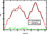
| [b2mt.pl](https://www.tbi.univie.ac.at/RNA/b2mt.1.html "View the manpage of the b2mt.pl perl script") | Produce a mountain representation of a secondary structure from it's [dot-bracket notation](https://www.tbi.univie.ac.at/RNA/documentation.html#dotbracket)
, as produced by `RNAfold`. Output consists of simple x y data suitable as input to a plotting program. The mountain representation is a xy plot with sequence position on the x-axis and the number of base pairs enclosing that position on the y-axis.
Example:
RNAfold < my.seq \| b2mt.pl \| xmgrace -pipe
[](https://www.tbi.univie.ac.at/RNA/gfx/5smnt.eps) |
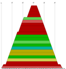
| [cmount.pl](https://www.tbi.univie.ac.at/RNA/cmount.1.html "View the manpage of the cmount.pl perl script") | Produce a PostScript mountain plot from a color dot plot as created by `RNAalifold -p` or `alidot -p`. Each base pair is represented by a trapez whose color encodes the number of consistent and compensatory mutations supporting that pair: Red marks pairs with no sequence variation; ochre, green, turquoise, blue, and violet mark pairs with 2,3,4,5,6 different types of pairs, respectively.
Example:
cmount.pl alidot.ps > cmount.ps
[](https://www.tbi.univie.ac.at/RNA/gfx/TAR_ss.ps) |
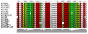
| [coloraln.pl](https://www.tbi.univie.ac.at/RNA/coloraln.1.html "View the manpage of the coloraln.pl perl script") | Reads a sequence alignment in CLUSTAL format and a consensus secondary structure (which it extracts from a secondary structure plot as produced by RNAalifold), and produces a postscript figure of the alignment annotated using the consensus structure, coloring base pair using the same color scheme as cmount.pl, RNAalifold and alidot.
Example:
coloraln.pl -s alirna.ps file.aln > coloraln.ps
[](https://www.tbi.univie.ac.at/RNA/gfx/TAR_aln.ps) |
| [colorrna.pl](https://www.tbi.univie.ac.at/RNA/colorrna.1.html "View the manpage of the colorrna.pl perl script") | Reads a consensus secondary structure plot and a color dot plot as produced by `RNAalifold -p`, and writes a new secondary structure plot in which base pairs a colored using the color information from the dot plot.
Example:
colorrna.pl alirna.ps alidot.ps > colorRNA.ps |
| [mountain.pl](https://www.tbi.univie.ac.at/RNA/mountain.1.html "View the manpage of the mountain.pl perl script") | Similar to `b2mt.pl`, but produces a mountain plot from the pair probabilities contained in a PostScript dot plot. It write 3 sets of x y data, suitable as input for a plot program. The first two sets containing the mountain representation from pair probabilities and MFE structure, the third set is the "positional entropy" a measure of structural well-definedness.
Example:
mountain.pl dot.ps \| xmgrace -pipe
[](https://www.tbi.univie.ac.at/RNA/gfx/TAR_cmt.eps) |
| [refold.pl](https://www.tbi.univie.ac.at/RNA/refold.1.html "View the manpage of the refold.pl perl script") | Refold using consensus structure as constraint |
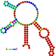
| [relplot.pl](https://www.tbi.univie.ac.at/RNA/relplot.1.html "View the manpage of the relplot.pl perl script") | Reads a postscript secondary structure plot and a dot plot containing pair probabilities as produced by `RNAfold -p`, and produces a new structure plot, color annotated with reliability information in the form of either pair probabilities or positional entropy (default).
Example:
relplot.pl foo\_ss.ps foo\_dp.ps > foo\_rss.ps
[](https://www.tbi.univie.ac.at/RNA/gfx/5srel.ps) |
| [rotate\_ss.pl](https://www.tbi.univie.ac.at/RNA/rotate_ss.1.html "View the manpage of the rotate_ss.pl perl script") | Reads a postscript secondary structure plot as produced by `RNAfold` and produces a new rotated and/or mirrored structure plot.
Example:
rotate\_ss.pl -a 30 -m foo\_ss.ps > foo\_new\_ss.ps |
| [switch.pl](https://www.tbi.univie.ac.at/RNA/switch.1.html "View the manpage of the switch.pl perl script") | Design sequences that can adopt two different structure, i.e. design RNA switches. The program will sample the set of sequences compatible with two input structures in order to find sequences with desired thermodynamic and kinetic properties. In particular it is possible to specify
1. Two different temperatures such that structure 1 is favored at T1 and structure 2 at T2 to design temperature sensitive switches (RNA thermometers)
2. The desired height of the energy barrier separating the two structures, thus determining the refolding time between meta-stable states. |
| [RNAdesign.pl](https://www.tbi.univie.ac.at/RNA/RNAdesign.1.html "View the manpage of the RNAdesign.pl perl script") | Flexible design of multi-stable RNA molecules. An initially random sequence is iteratively mutated and evaluated according to an objective function (see Option: `--optfun`). Whenever a better scoring sequence has been found, the mutation is accepted, the algorithm terminates once a local minimum is found. This script makes heavy use of the new `RNA::Design` Perl 5 sub-package provided by the latest ViennaRNA Package. |
### RNAlib Reference Manual
The core of the ViennaRNA Package is formed by a collection of routines for the prediction and comparison of RNA secondary structures. These routines can be accessed through the stand-alone programs and utilities described above, which should be sufficient for most users. For those who wish to develop their own programs we provide a library that can either be linked to your own C/C++ code, or accessed through our scripting language interface. Currently, we provide support for Perl and Python.
Follow [this link](https://www.tbi.univie.ac.at/RNA/ViennaRNA/refman/index.html)
to view the HTML version of the **RNAlib** API Reference Manual.
 The documentation can also be [downloaded as a PDF document](https://www.tbi.univie.ac.at/RNA/ViennaRNA/doc/RNAlib-2.7.0.pdf)
The documentation can also be found at [Read the Docs](https://viennarna.readthedocs.io/)
### Terms and Definitions
Throughout these webpages, we use many terms related to RNA secondary structure prediction. Below you'll find a list of some often used vocabulary and its corresponding definition.
| Term | Description |
| --- | --- |
| Dot-Bracket notation | Pseudo-knot free secondary structures can be represented in the space-efficient _bracket notation_, which is used throughout the ViennaRNA package. A structure on a sequence of length n is represented by a string of equal length consisting of matching brackets and dots. A base pair between base i and j is represented by a `(` at position i and a `)` at position j, unpaired bases are represented by dots. Thus the secondary structure
(((..((((...)))).)))
is equivalent to:
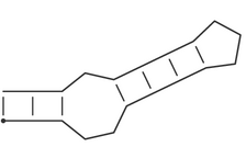
i.e. a stem-loop structure consisting of a an outer helix of 3 base pairs followed by an interior loop of size 3, a second helix of length 4, and a hairpin loop of size 3.
Base pair probabilities are sometimes summarized in pseudo bracket notation with the additional symbols `,`, `\|`, `{`, `}`. Here, the usual `(`, `)`, `.`, represent bases with a strong preference (more than 2/3) to pair upstream (with a partner further 3'), pair down-stream, or not pair, respectively. `{`, `}`, and `,` are just weaker version of the above and `\|` represents a base that is mostly paired but has pairing partners both upstream and downstream. In this case open and closed brackets need not match up. |
### Comments and Bug Reports
If in doubt our program is right, nature is at fault.
Comments and bug reports should be sent to [rna@tbi.univie.ac.at](mailto:rna@tbi.univie.ac.at)
---
# RNAz
RNAz - predicting structural noncoding RNAs
===========================================
* [Introduction](https://www.tbi.univie.ac.at/~wash/RNAz/#introduction)
* [News](https://www.tbi.univie.ac.at/~wash/RNAz/#news)
* [Download](https://www.tbi.univie.ac.at/~wash/RNAz/#download)
* [Getting started](https://www.tbi.univie.ac.at/~wash/RNAz/#started)
* [Documentation](https://www.tbi.univie.ac.at/~wash/RNAz/#documentation)
* [Links](https://www.tbi.univie.ac.at/~wash/RNAz/#links)
* [Contact](https://www.tbi.univie.ac.at/~wash/RNAz/#contact)
* [Visit our **RNAz web-server**!](http://rna.tbi.univie.ac.at/)
Introduction
------------
RNAz is a program for predicting structurally conserved and thermodynamically stable RNA secondary structures in multiple sequence alignments. It can be used in genome wide screens to detect functional RNA structures, as found in noncoding RNAs and cis-acting regulatory elements of mRNAs.
The method is described in:
Washietl S., Hofacker I.L., Stadler P.F.
[Fast and reliable prediction of noncoding RNAs](http://www.pnas.org/cgi/content/abstract/0409169102v1)
_Proc. Natl. Acad. Sci. U.S.A._ **102**: 2454-2459, 2005
[RNAz 2.0: Improved noncoding RNA detection](http://eproceedings.worldscinet.com/9789814295291/9789814295291_0009.html)
Gruber AR, Findeiß S, Washietl S, Hofacker IL, Stadler PF. _Pac Symp Biocomput._ **15**:69-79, 2010
News
----
**2011-10-06** RNAz version 2.1 is released. Some minor bug fixes and simplified command line options with more practical defaults. Also the [documentation](https://www.tbi.univie.ac.at/~wash/RNAz/#documentation)
has been extended and updated.
**2009-09-21** A pre-release of the new version 2.0 of RNAz is available. Among other additions, this new release features improved z-score estimates based on a dinucleotide model, a new classfication model built from a singificantly bigger test set and classfication model for structurally aligned sequences. The improvements are described in an upcoming Manuscript: Gruber et al. "RNAz 2.0: improved noncoding RNA detection" PSB 2010.
**2008-04-07** A novel method to estimate the false discovery rate of RNAz is available. Instead of using a simplistic shuffling algorithm to randomize alignments, SISSIz simulates random alignments preserving dinucleotide content. The algorithm is described in [this paper](http://www.biomedcentral.com/1471-2105/9/248)
and the program can be downloaded here: [http://sourceforge.net/projects/sissiz](http://sourceforge.net/projects/sissiz/)
**2007-02-06** Our new RNAz web server is available here: [rna.tbi.univie.ac.at/RNAz](http://rna.tbi.univie.ac.at/RNAz)
. It allows to analyze your sequences online without installing any software on your computer.
**2006-10-13** RNAz 1.0 is available. A series of bugs have been fixed, most prominently the bug that caused the program to crash on 64 bit machines. _If you are using a 64 bit machine make sure that you use the latest version!_ Thanks to all people who have reported bugs.
**2006-03-28** A pre-release for the new version RNAz 1.0 is available. There are no major changes in the algorithm compared to the previous version. However, the user interface of RNAz has been improved. Most notably a set of Perl helper programs is available that implement a complete analysis pipeline suitable for large scale screens. See [NEWS](https://www.tbi.univie.ac.at/~wash/RNAz/NEWS.txt)
for a complete list of changes. Please note: I will call the current version \`\`pre-release" for a while just to make sure that I can fix potential bugs before I finally name it \`\`1.0". Also note the new **[Manual/Tutorial](https://www.tbi.univie.ac.at/~wash/RNAz/manual.pdf)
**!
Download
--------
| Version | Date | File | Platform | Package type |
| --- | --- | --- | --- | --- |
| 2.1 | 10/06/2011 | [RNAz-2.1.tar.gz](https://www.tbi.univie.ac.at/~wash/RNAz/RNAz-2.1.tar.gz) | Linux/Unix/OSX | Source |
| 1.0 | 10/13/2006 | [RNAz-1.0-win32.msi](https://www.tbi.univie.ac.at/~wash/RNAz/RNAz-1.0-win32.msi) | Windows | Binary |
[Old versions](https://www.tbi.univie.ac.at/~wash/RNAz/old_versions.html)
The latest source code is available at [https://github.com/wash/rnaz](https://github.com/wash/rnaz)
Getting started
---------------
### Linux / Unix / OSX
The following installation procedure should work on all Unix-like systems. On OS X it is necessary that you have installed the \`\`XCode" tools.
Download the latest RNAz-X.X-tar.gz and run the following commands:
tar -xzf RNAz-X.X-tar.gz
cd RNAz-X.X
./configure
make
make install
The last step requires root privileges and installs the RNAz files into the /usr/local/ tree. The executable is for example installed to /usr/local/bin and you should now be able to run the program which you can easily check by typing RNAz --version.
If you do not have root privileges on your system or prefer to install RNAz into a self-contained directory run configure for example like this:
./configure --prefix=/myhome/RNAz --datadir=/myhome/RNAz/share
The Perl programs are by default installed to /usr/local/share/RNAz/perl/. They are not installed by default since different people like their scripts in different locations. So copy all files from this directory to your favourite directory which is in your PATH of executables. For example copy them to /usr/local/bin:
cp /usr/local/share/RNAz/perl/\* /usr/local/bin
Alternatively you can add this directory to your PATH.
### MS Windows
_**Note:** The windows support has been discontinued as of version 2.0. The windows package for version 1.0 is still available._
Simply download the latest RNAz-X.X-win32.msi file and double click it. Follow the instructions. Open a console window and type RNAz --version to test your installation.
The Perl programs are also automatically installed. To run them you need to have installed ActivePerl. Get the latest msi-installer package from [www.activestate.com](http://www.activestate.com/)
and follow the instructions. Make sure that you choose \`\`Add Perl to PATH environment variable" and \`\`Create Perl file extension association" during installation.
### Testing RNAz
You can test RNAz on one of the example alignments (default location under Unix/Linux/OSX: /usr/local/share/RNAz/examples, Windows: c:\\Program Files\\RNAz\\examples):
cd /usr/local/share/RNAz/examples
RNAz tRNA.aln
To test if the Perl programs work run for example:
rnazWindow.pl --window=120 --slide=40 unknown.aln | RNAz
Documentation
-------------
A manual/tutorial for using RNAz and helper programs is available here: **[manual.pdf](https://www.tbi.univie.ac.at/~wash/RNAz/manual.pdf)
**
Manual pages are also available here:
* [**RNAz**](https://www.tbi.univie.ac.at/~wash/RNAz/man/RNAz.html)
* [rnazWindow.pl](https://www.tbi.univie.ac.at/~wash/RNAz/man/rnazWindow.html)
* [rnazOutputSort.pl](https://www.tbi.univie.ac.at/~wash/RNAz/man/rnazOutputSort.html)
* [rnazCluster.pl](https://www.tbi.univie.ac.at/~wash/RNAz/man/rnazCluster.html)
* [rnazFilter.pl](https://www.tbi.univie.ac.at/~wash/RNAz/man/rnazFilter.html)
* [rnazSort.pl](https://www.tbi.univie.ac.at/~wash/RNAz/man/rnazSort.html)
* [rnazAnnotate.pl](https://www.tbi.univie.ac.at/~wash/RNAz/man/rnazAnnotate.html)
* [rnazBlast.pl](https://www.tbi.univie.ac.at/~wash/RNAz/man/rnazBlast.html)
* [rnazCMsearch.pl](https://www.tbi.univie.ac.at/~wash/RNAz/man/rnazCMsearch.html)
* [rnazIndex.pl](https://www.tbi.univie.ac.at/~wash/RNAz/man/rnazIndex.html)
* [rnazBEDsort.pl](https://www.tbi.univie.ac.at/~wash/RNAz/man/rnazBEDsort.html)
* [rnazBEDstats.pl](https://www.tbi.univie.ac.at/~wash/RNAz/man/rnazBEDstats.html)
* [rnazMAF2BED.pl](https://www.tbi.univie.ac.at/~wash/RNAz/man/rnazMAF2BED.html)
* [rnazRandomizeAln.pl](https://www.tbi.univie.ac.at/~wash/RNAz/man/rnazRandomizeAln.html)
Links
-----
If you are interested in RNAz you might also be interested in ...
* [QRNA](http://selab.janelia.org/software#qrna)
* [EvoFold](http://www.cbse.ucsc.edu/~jsp/EvoFold/)
* [CMFinder](http://bio.cs.washington.edu/yzizhen/CMfinder/)
* [RNAcode](http://wash.github.com/rnacode/)
Contact
-------
Please feel free to contact [us](mailto:rna@tbi.univie.ac.at)
for comments, bug-reports etc.
[rna@tbi.univie.ac.at](mailto:rna@tbi.univie.ac.at)
Last modified: Thu Oct 06 2011
---
# Extended RNA Secondary Structures - RNAwolf
RNAwolf
-------
[Home](http://www.tbi.univie.ac.at/software/rnawolf/index.html)
[News](http://www.tbi.univie.ac.at/software/rnawolf/news.html)
[RNAwolf](http://www.tbi.univie.ac.at/software/rnawolf/rnawolf.html)
[MC-Fold-DP](http://www.tbi.univie.ac.at/software/rnawolf/mcfolddp.html)
[SSPcompare](http://www.tbi.univie.ac.at/software/rnawolf/sspcompare.html)
[Downloads](http://www.tbi.univie.ac.at/software/rnawolf/download.html)
[how to cite](http://www.tbi.univie.ac.at/software/rnawolf/citation.html)
Introduction
------------
**RNAwolf** (and additional tools) is designed to predict _extended RNA secondary structure_ and the main tool described in Höner zu Siederdissen et al. (2011) . An extended structure is allowed to contain non-canonical base-pairs and structures composed of 2-diagrams. The allowed base-pairs can contain all 4x4 nucleotides and the nucleotide bonds are explicitly annotated with the paired edges and isomerism information. 2-diagrams are required to describe structures were a nucleotide may be involved in more than one base pair. In principle, each nucleotide may be involved in up to three interactions, but as those are rarely annotated currently, we restrict ourselves to two. If required, the extension to three nucleotides is straightforward.
As with other algorithms (e.g. **MC-Fold-DP**), the grammar behind **RNAwolf** is unambiguous. This allows for exhaustive enumeration of all structures within a certain band above the optimal structure (or simply all co-optimal structures).
Using RNAwolf
-------------
#### Basic usage
The basic principle is the same as with **RNAfold**:
echo CCCAAAGGG | ./RNAwolf
This returns an extended secondary structure. The structure or structures can be converted into postscript figures using a supplied perl script. Further options will be provided soon.
#### Constrained folding
This will fold the sequence, given certain structural constraints:
echo CCCAAAGGG | ./RNAwolf --constraint "(...x...)"
Normal brackets `()` force a pairing, `x` disallows this nucleotide from pairing, while `.` means that the nucleotide may fold without restrictions.
Parameter optimization
----------------------
### Running RNAwolf in parameter optimization mode
This is basically a two-step procedure:
1. create training data from RNAstrand (Andronescu et al. 2008) or FR3D (Sarver et al. 2008) using **RNAwolfTrainingData**. FR3D has an advantage compared to the "raw PDB" as the task of parsing PDB has already been done.
2. follow the same steps as in scripts/run.sh (or in scripts/sge)
### Sun Grid Engine compatibility
The package comes with a sub-directory for scripts. In scripts/sge are three scripts that work in conjunction with the Sun Grid Engine. We currently support parallelizing the folding process (**RNAwolf**) but not parameter optimization. This is typically acceptable, as folding takes much more time than optimizing.
The scripts need to be fixed up to work on your systems, grap the xstat and xsub scripts as well, if needed.
### References
Andronescu, Mirela, Vera Bereg, Holger Hoos, and Anne Condon. 2008. RNA STRAND: The RNA Secondary Structure and Statistical Analysis Database. _BMC Bioinformatics_ 9: 340. doi:10.1186/1471-2105-9-340. http://www.biomedcentral.com/1471-2105/9/340.
Höner zu Siederdissen, Christian, Stephan H. Bernhart, Peter F. Stadler, and Ivo L. Hofacker. 2011. A Folding Algorithm for Extended RNA Secondary Structures. _Bioinformatics_ 27: 129–36. doi:10.1093/bioinformatics/btr220.
Sarver, Michael, Craig L. Zirbel, Jesse Stombaugh, Ali Mokdad, and Neocles B. Leontis. 2008. FR3D: Finding Local and Composite Recurrent Structural Motifs in RNA 3D Structures. _Journal of Mathematical Biology_: 215–52.
---
# Unknown
RNAz 2.1 Predicting structural noncoding RNAs Stefan Washietl Department for Theoretical Chemistry University Vienna wash@tbi.univie.ac.at http://www.tbi.univie.ac.at/ ̃ wash/RNAz Contentsi Contents 1Introduction1 1.1Prediction of noncoding RNAs . . . . . . . . . . . . . . . . . . . .1 1.2The RNAz approach . . . . . . . . . . . . . . . . . . . . . . . . .2 1.2.1Thermodynamic stability . . . . . . . . . . . . . . . . . . .2 1.2.2Structural conservation . . . . . . . . . . . . . . . . . . . .2 1.2.3Putting it together . . . . . . . . . . . . . . . . . . . . . . .2 1.3General remarks and typographical conventions . . . . . . .. . . .3 2Materials3 2.1Hardware . . . . . . . . . . . . . . . . . . . . . . . . . . . . . . .3 2.2Operating system . . . . . . . . . . . . . . . . . . . . . . . . . . .3 2.3Perl . . . . . . . . . . . . . . . . . . . . . . . . . . . . . . . . . .4 2.4RNAz . . . . . . . . . . . . . . . . . . . . . . . . . . . . . . . . .4 2.5Optional software . . . . . . . . . . . . . . . . . . . . . . . . . . .4 2.6Example files . . . . . . . . . . . . . . . . . . . . . . . . . . . . .4 3Methods4 3.1Installation of RNAz . . . . . . . . . . . . . . . . . . . . . . . . .4 3.1.1Linux/UNIX and OS X . . . . . . . . . . . . . . . . . . . .4 3.2Installation of optional Software . . . . . . . . . . . . . . . . . ..5 3.3Installation of example files . . . . . . . . . . . . . . . . . . . . . .6 3.4Basic usage of RNAz . . . . . . . . . . . . . . . . . . . . . . . . .6 3.4.1Input alignment . . . . . . . . . . . . . . . . . . . . . . . .6 3.4.2Running RNAz . . . . . . . . . . . . . . . . . . . . . . . .8 3.4.3Understanding the output . . . . . . . . . . . . . . . . . . .8 3.5Advanced usage of RNAz . . . . . . . . . . . . . . . . . . . . . . . 10 Contentsii 3.5.1Analyzing forward and reverse strand . . . . . . . . . . . . 10 3.5.2Scoring long alignments . . . . . . . . . . . . . . . . . . . 10 3.5.3Selecting subsets of sequences . . . . . . . . . . . . . . . . 10 3.5.4Visualizing the results . . . . . . . . . . . . . . . . . . . . 11 3.6Large scale genomic screens . . . . . . . . . . . . . . . . . . . . . 12 3.6.1Overview . . . . . . . . . . . . . . . . . . . . . . . . . . . 12 3.6.2Choosing raw input alignments . . . . . . . . . . . . . . . 12 3.6.3Pre-processing raw alignments . . . . . . . . . . . . . . . . 12 3.6.4Running RNAz . . . . . . . . . . . . . . . . . . . . . . . . 14 3.6.5Clustering the results . . . . . . . . . . . . . . . . . . . . . 14 3.6.6Filtering and sorting the results . . . . . . . . . . . . . . . 15 3.6.7Exporting the results to standard annotation formats. . . . 15 3.6.8Visualizing the results on a website . . . . . . . . . . . . . 16 3.6.9Comparing hits to known annotation . . . . . . . . . . . . . 16 3.6.10 Annotating hits with database search . . . . . . . . . . . . .17 3.6.11 Estimating false positives and gathering statistics . . . . . . 18 4Notes19 4.1Custom installation of RNAz . . . . . . . . . . . . . . . . . . . . . 19 4.2Running the Perl programs . . . . . . . . . . . . . . . . . . . . . . 19 4.3Creating the input alignments . . . . . . . . . . . . . . . . . . . . . 20 4.4Additional output values . . . . . . . . . . . . . . . . . . . . . . . 20 4.5Estimating false positives . . . . . . . . . . . . . . . . . . . . . . . 21 4.6Manual inspection of candidates . . . . . . . . . . . . . . . . . . . 21 4.7Advanced filtering . . . . . . . . . . . . . . . . . . . . . . . . . . . 22 A Manual pages25 A.1RNAz. . . . . . . . . . . . . . . . . . . . . . . . . . . . . . . . . 25 Contentsiii A.2rnazWindow.pl. . . . . . . . . . . . . . . . . . . . . . . . . . 27 A.3rnazOutputSort.pl. . . . . . . . . . . . . . . . . . . . . . . 30 A.4rnazCluster.pl. . . . . . . . . . . . . . . . . . . . . . . . . 31 A.5rnazSelectSeqs.pl. . . . . . . . . . . . . . . . . . . . . . . 35 A.6rnazFilter.pl. . . . . . . . . . . . . . . . . . . . . . . . . . 37 A.7rnazSort.pl. . . . . . . . . . . . . . . . . . . . . . . . . . . . 40 A.8rnazAnnotate.pl. . . . . . . . . . . . . . . . . . . . . . . . 43 A.9rnazBlast.pl. . . . . . . . . . . . . . . . . . . . . . . . . . . 44 A.10rnazCmsearch.pl. . . . . . . . . . . . . . . . . . . . . . . . 46 A.11rnazIndex.pl. . . . . . . . . . . . . . . . . . . . . . . . . . . 48 A.12rnazBEDsort.pl. . . . . . . . . . . . . . . . . . . . . . . . . 51 A.13rnazBEDstats.pl. . . . . . . . . . . . . . . . . . . . . . . . 52 A.14rnazMAF2BED.pl. . . . . . . . . . . . . . . . . . . . . . . . . 53 A.15rnazRandomizeAln.pl. . . . . . . . . . . . . . . . . . . . . 55 Contentsiv Preface The function of many noncoding RNAs (ncRNAs) depend on a definedsecondary structure. RNAz detects evolutionary conserved and thermodynamically stable RNA secondary structures in multiple sequence alignments and thus efficiently filters for candidate ncRNAs. There are two main goals of this document. First, it should give detailed technical advice on how to use RNAz. Second, it should help you to get a well-founded understanding of the results you get from RNA leading to reasonable conclusions for your application. This document is largely based on a draft for a book chapter and it is thus organized in an idiosyncratic way. Until there is more time to write a dedicated tutorial and manual I will keep this organization. I start with a short introduction to the problem ofde novoprediction of ncRNAs and the RNAz algorithm. In the next part, I will explain how to install RNAz and all necessary helper programs on your system. Next, I demonstrate the basic usage of RNAz including the correct formatting of the input alignments. More advanced techniques which require pre-processing steps of the inputalignments are discussed afterwards. In the last section, I show how to conduct a RNAz screen of a large num- ber of automatically generated alignments on the example ofgenome-wide screen ofSaccharomyces cerevisiae. The theory behind RNAz is described in more detail in reference \[18\]. Improve- ments made in version 2.0 are described in reference \[7\]. If you are interested in RNAz for the purpose of annotating noncoding RNAs, our new program RNAcode \[3\] might be of interest. It was developed to be used in combination with RNAz and evaluates the protein coding potential of candidate ncRNAs. Stefan Washietl 1. Introduction1 1 Introduction 1.1 Prediction of noncoding RNAs In contrast to protein-gene finders which are routinely usedfor genome annotation, noncoding RNA (ncRNA) gene finders are still in their infancy. The main reason that hinders systematicde novoprediction of ncRNAs is that there are no common statistically significant features in primary sequence (e.g. open reading frames or codon bias) which could be exploited for efficient algorithms. It is even not clear what we define as “ncRNA”. There is no doubt that indepen- dent “RNA genes” with a defined molecular function such as tRNAs, microRNAs, or snoRNAs should be called ncRNAs. But the situation is not always that clear. The transcriptional activity of at least mammalian genomesis much more com- plex than anticipated \[4\]. We see mRNA-like ncRNAs, non-polyadenylated RNAs from both intronic and intergenic regions, overlapping transcripts, extensive anti- sense transcription, and transcribed protein-pseudogenes. In addition, there is a recent example of a noncoding transcript that only is expressed to interfere with and downregulate the transcription of a neighboring gene but the produced RNA molecule itself does not have any obvious function \[11\]. There is even an example of a functional RNA encoding a protein \[1\]. The spectrum of ncRNAs and their mode of action is very heterogeneous. One can safely assume that the full spec- trum of functions is not yet discovered and that a general ncRNA gene finder is an unrealistic goal even in the long term. However, there is a subclass of ncRNAs which — with the help of comparative genomics — can be predicted with fair accuracy.StructuralncRNAs have a defined and evolutionary conserved secondary structure which is offunctional importance. Most of the well known “classical” ncRNAs, as for example tRNA,rRNA, RNAse P, or SRP RNA, are of this class. Pioneering work in the prediction of structural ncRNAs by comparative genomics was done by Rivas & Eddy. QRNA predicts conserved RNA secondary structures on pairwise alignments using a probabilistic approach based on a stochastic context free grammar to modelRNA structure \[13, 14, 12\]. RNAz \[18\] takes a different approach. It is based on minimum free energy (MFE) structure prediction algorithms \[19, 9\]. It relies onthe fact that structural RNAs have two characteristic features: (i) unusual thermodynamic stability and (ii) conservation of secondary structure. The following section outlines the basic principles of RNAz. 1. Introduction2 1.2 The RNAz approach 1.2.1 Thermodynamic stability It is easy to calculate the MFE as a measure of thermodynamic stability for a se- quence using e.g. RNAfold \[9\]. However, the MFE depends on thelength and the base composition of the sequence and is, therefore, difficult to interpret in absolute terms. RNAz calculates a normalized measure of thermodynamic stability by com- paring the MFEmof a given (native) sequence to the MFEs of a large number of random sequences of the same length and base composition. Az-score is calculated asz= (m−μ)/σ, whereμandσare the mean and standard deviations, resp., of the MFEs of the random samples. Negativez-scores indicate that a sequence is more stable than expected by chance. RNAz does not actually samplerandom sequences but approximatesz-scores, which is much faster but of the same accuracy. 1.2.2 Structural conservation RNAz predicts a consensus secondary structure for an alignment by using the RNAal- ifold approach \[8\]. RNAalifold works almost exactly as single sequence folding algorithms (e.g. RNAfold), with the main difference that theenergy model is aug- mented by covariance information. Compensatory mutations (e.g. a CG pair mu- tates to a UA pair) and consistent mutations (e.g. AU mutatesto GU) give a “bonus” energy while inconsistent mutations (e.g. CG mutates to CA) yield a penalty. This results in aconsensusMFEE A . RNAz compares this consensus MFE to theav- erageMFE of the individual sequences ̄ Eand calculates a structure conservation index: SCI=E A / ̄ E. The SCI will be high if the sequences fold together equally well as if folded individually. On the other hand, SCI will be low if no consensus fold can be found. 1.2.3 Putting it together The two independent diagnostic features of structural ncRNAs,z-score and SCI, are finally used to classify an alignment as “structural RNA” or “other”. For this purpose, RNAz uses a support vector machine (SVM) learning algorithm which is trained an a large test set of well known ncRNAs. Using RNAz, it is possible to efficiently screen alignments for functional RNA sec- ondary structures. It is important to note that RNAz cannot distinguish functional RNA elements which are part of ncRNAs from elements which arecis-regulatory elements of mRNAs. 2. Materials3 1.3 General remarks and typographical conventions There is no graphical user interface for RNAz. All steps are carried out on a command-line (terminal). Lines starting with a “#” are commands and you should type them into your terminal window, followed by pressing return. The “#” sign stands for your command line prompt and may look different onyour system. If a command is too long for one line in this book it is separated bya backslash “\\” and continues on the next line. Donotinput the backslash, simply type in the command on one line. All programs are implemented as filters, i.e. they read from the standard input and write to the standard output. Therefore, we make use of the pipe (“|”) and redirection operators (“<”,”>”). You can get a online documentation on the usage of each program by using the --helpoption, e.g.: # RNAz --help For the Perl programs you get more detailed manual pages by using the--man option. All manual pages are reproduced in Appendix A in thismanual. Most command line options have a long (e.g.--help) and a short (e.g.-h) form. For didactic reasons, we use long option names throughout this manual. 2 Materials 2.1 Hardware RNAz is generally fast. Small to medium sized data sets, as forexample the yeast screen in section 3.6, can be analyzed within reasonable time on a single modern desktop or even laptop computer. 2.2 Operating system If available, we recommend to use a Linux/UNIX system for your analysis. Also Mac OS X, in principle a full featured UNIX system, is an adaequate platform. Note: We have discontinued the Windows version of RNAz as of version 2.0 3. Methods4 2.3 Perl The RNAz program is bundled with a variety of helper programs which are written in the Perl programming language. To run these programs you need to have installed Perl on your system, which is most likely the case on all Linux/UNIX systems and on Mac OS X. 2.4 RNAz The RNAz program can be downloaded from:www.tbi.univie.ac.at/ ̃ wash/RNAz. For the examples in this manual, RNAz version 1.0 was used. ForLinux/UNIX and OS X, download the fileRNAz-2.0.tar.gz. 2.5 Optional software Some advanced analysis steps (sections 3.6.8 and 3.6.10) require additional soft- ware to be installed on your system. To create HTML formatted output of the results as described in section 3.6.8 you will need to have installed the Vienna RNA package (www.tbi.univie.ac.at/RNA) and the postscript interpreter Ghostscript (http://www.cs.wisc.edu/ ̃ ghost/). To perform automatic database searches of predicted ncRNA candidates you need NCBI Blast (ftp://ftp.ncbi.nih.gov/blast). 2.6 Example files Most of the example files used in this manual are part of the RNAzpackage. If you want to reproduce theS. cerevisiaescreen described in section 3.6 you can down- load the data file from:www.tbi.univie.ac.at/papers/SUPPLEMENTS/MiMB/. 3 Methods 3.1 Installation of RNAz 3.1.1 Linux/UNIX and OS X In the simplest case you can run the following series of commands to build and install RNAz: 3. Methods5 # tar -xzf RNAz-1.0.tar.gz # cd RNAz-1.0 # ./configure # make # su # make install This requires root privileges and installs all files under the/usr/localtree. The RNAzexecutable is installed in/usr/local/binand you should now be able to run the program (tryRNAz --versionon a terminal window). If you do not have root privileges or experience other problems (e.g.gcccompiler not found) see note 4.1. The Perl programs are installed to/usr/local/share/RNAz/perl. To make these programs available from other locations you can either add this directory to yourPATHof executables environment variable or copy the Perl programs to an existing directory already in yourPATH. In case you are not familiar on how to run Perl programs refer to note 4.2. 3.2 Installation of optional Software We cannot cover in detail the installation procedure of the optional software. We just give an outline how to install the Vienna RNA package and NCBI blast on a standard Linux system. Together with an existing Ghostscript installation, this will allow you to run the examples in sections 3.6.8 and 3.6.10. To install the Vienna RNA package, get the latestViennaRNA-X.X.tar.gz file fromwww.tbi.univie.ac.at/RNA. The package can be installed in ex- actly the same way as RNAz, using./configureandmake. Please refer to theINSTALLdocument for detailed installation options. Make sure thatthe Perl programs in theUtilsdirectory are in yourPATHof executables. To install NCBI Blast download theblast-2. \* .tar.gz-package matching your platform fromftp://ftp.ncbi.nih.gov/blast/executables/LATEST/. Copy it to an installation directory of your choice and “untar” it. The executables are located in thebinsubdirectory which you should add to yourPATHvariable. You can install the Vienna RNA package and NCBI Blast without problems on OS X by following the instructions above. However, unlike ona Linux system, Ghostscript is not installed per default. You can try to get apre-compiled package fromfink.sourceforge.netordarwinports.opendarwin.org. Al- ternatively, you can download the source fromhttp://www.ghostscript.com/ and build the package with./configureandmake. 3. Methods6 3.3 Installation of example files Move the example fileyeast-examples.tar.gzto a directory of your choice and “untar” the file: # tar -xzf yeast-examples.tar.gz 3.4 Basic usage of RNAz 3.4.1 Input alignment RNAz takes a multiple sequence alignment as input. RNAz doesnotalign se- quences, so you have to use other programs for creating your alignments. If you prepare your alignments manually (in contrast to automaticgenome-wide align- ments as in section 3.6) we recommend using Clustal W \[16\]. It is an easy-to-use and widely available tool which performs well on structuralRNAs \[5\]. For hints on preparing the alignments see note 4.3. RNAz can read two different alignment formats: Clustal W (Fig.1A) and MAF (Fig. 1B). The Clustal W format is a concise format which is supported by many programs and thus suitable for every-day use. For genomic screens, however, it is necessary to exactly store the genomic locations of aligned sequences. For this purpose, the MAF format was developed which requires six fields for each sequence entry: 1. a unique identifier of the source sequence, 2. the start position of the aligned subsequence with respect to this source se- quence, 3. the length of the aligned subsequence without gaps, 4. “+” or “-” indicating if the sequence is in the same readingdirection of the source sequence or the reverse complement, 5. the sequence length of the complete source sequence, 6. the aligned subsequence with gaps. The full specification of the format can be found here:http://genome.ucsc.edu/goldenPath/help/maf.html It should be noted that RNAz and all other helper programs do not make use of field 5 and also ignore the value of the “score=” field in the header line. So it is possi- ble to simply fill these fields with 0 or any other arbitrary values, if the real values are not easily available. 3. Methods7 CLUSTAL W (1.83) multiple sequence alignment sacCer1 GCCTTGTTGGCGCAATCGGTAGCGCGTATGACTCTTAATCATAAGGTTAGGGGTTCGAGC sacBay GCCTTGTTGGCGCAATCGGTAGCGCGTATGACTCTTAATCATAAGGTTAGGGGTTCGAGC sacKlu GCCTTGTTGGCGCAATCGGTAGCGCGTATGACTCTTAATCATAAGGCTAGGGGTTCGAGC sacCas GCTTCAGTAGCTCAGTCGGAAGAGCGTCAGTCTCATAATCTGAAGGTCGAGAGTTCGAAC \*\* \* \* \*\* \*\* \*\*\*\* \*\* \*\*\*\* \* \*\*\* \*\*\*\*\* \*\*\*\* \* \*\*\*\*\*\* \* sacCer1 CCCCTACAGGGCT sacBay CCCCTACAGGGCT sacKlu CCCCTACAGGGCT sacCas CTCCCCTGGAGCA \* \*\* \* \*\* ########################### RNAz 0.1.1 ############################# Sequences: 4 Columns: 73 Reading direction: forward Mean pairwise identity: 80.82 Mean single sequence MFE: -27.20 Consensus MFE: -26.50 Energy contribution: -23.62 Covariance contribution: -2.88 Combinations/Pair: 1.43 Mean z-score: -2.18 Structure conservation index: 0.97 SVM decision value: 2.39 SVM RNA-class probability: 0.993311 Prediction: RNA ###################################################################### >sacCer1.chr4 1352453 73 - 1531914 GCCUUGUUGGCGCAAUCGGUAGCGCGUAUGACUCUUAAUCAUAAGGUUAGGGGUUCGAGCCCCCUACAGGGCU (((((((.(((((........))))...((((.((((....))))))))(((((....)))))).))))))). ( -29.20) >sacBay.contig\_465 14962 73 - 57401 GCCUUGUUGGCGCAAUCGGUAGCGCGUAUGACUCUUAAUCAUAAGGUUAGGGGUUCGAGCCCCCUACAGGGCU (((((((.(((((........))))...((((.((((....))))))))(((((....)))))).))))))). ( -29.20) >sacKlu.Contig1694 137 73 + 4878 GCCUUGUUGGCGCAAUCGGUAGCGCGUAUGACUCUUAAUCAUAAGGCUAGGGGUUCGAGCCCCCUACAGGGCU (((((((.(((((........)))).(((((.......)))))......(((((....)))))).))))))). ( -27.20) >sacCas.Contig128 258 73 + 663 GCUUCAGUAGCUCAGUCGGAAGAGCGUCAGUCUCAUAAUCUGAAGGUCGAGAGUUCGAACCUCCCCUGGAGCA (((((((..((((........)))).((((.........))))((((((......)).))))...))))))). ( -23.20) >consensus GCCUUGUUGGCGCAAUCGGUAGCGCGUAUGACUCUUAAUCAUAAGGUUAGGGGUUCGAGCCCCCUACAGGGCU (((((((..((((........)))).(((((.......))))).....(((((.......)))))))))))). (-26.50 = -23.62 + -2.88) ##maf version=1 a score=119673.000000 s sacCer1.chr4 1352453 73 - 1531914 GCCTTGTTGGCGCAATCGGTAGCGCGTATGACTCTT... s sacBay.contig\_465 14962 73 - 57401 GCCTTGTTGGCGCAATCGGTAGCGCGTATGACTCTT... s sacKlu.Contig1694 137 73 + 4878 GCCTTGTTGGCGCAATCGGTAGCGCGTATGACTCTT... s sacCas.Contig128 258 73 + 663 GCTTCAGTAGCTCAGTCGGAAGAGCGTCAGTCTCAT... A B C Fig. 1.Supported alignment formats and RNAz output. (A) Clustal W format, (B) MAF format (sequences have been shortened due to space restrictions), (C) Output of RNAz on the MAF file shown in (B). 3. Methods8 The RNAz package contains several example files which are by default installed to/usr/local/share/RNAz/examples. To run the following examples change into this directory. 3.4.2 Running RNAz As soon you have prepared your alignment you can immediatelyscore it with RNAz. In the simplest case you type: # RNAz tRNA.maf The filetRNA.mafis that one shown in Fig. 1B and the command gives you the output shown in Fig. 1C. 3.4.3 Understanding the output As described in the introduction, RNAz calculates various folding characteristics to classify the alignment. These are displayed in the headersection of the RNAz output. The mean single MFE is compared to the consensus MFE which results in the SCI, a measure for structural conservation (section 1.2.2). In this ideal example of a tRNA, we observe a very high SCI of 0.97. The SCI depends on the mean pair- wise identity and the number of sequences in the alignment. So, it is not possible interpret the significance of a SCI-value in absolute terms. As a rule of thumb, a SCI near or even above the mean pairwise identity is “good” andmight indicate structural conservation. For example, given an alignment with five sequences and a mean pairwise identity of 60%, a SCI of 0.75 can be regarded asstrong hint for a conserved fold. On the other hand, on a pairwise alignment with 90% identity, SCI=0.75 does not indicate a conserved fold at all. The second characteristic is thermodynamic stability, which is expressed as the meanz-score of the sequences in the alignment (see section 1.2.1).z-scores of MFEs are not exactly normal distributed, so you cannot directly give a statistical significance for yourz-score. However, meanz-scores below−3or−4generally indicate very stable structures, that should arise only in rare cases by chance. Also here, one has to consider the overall sequence divergence inthe alignment. On a pairwise alignment with 90% identity az-score of−4is much more likely to occur by chance than on an alignment of six sequences with only 60% identity. Apart from SCI andz-score, there are a few other values displayed in the RNAz output. If you are wondering what they mean, see note 4.4. 3. Methods9 RNAz assists you in the final classification by providing an overall “RNA-class probability”, or “P-value”. It is important to know that this isnotaP-value in a strict statistical sense, simply because there is no underlying statistical model. Instead, RNAz uses a ratherad hocmachine learning technique to calculate this value. IfP >0.5, the alignment is classified as “RNA”. The false positive rate at this cutoff was found to be≈4%, i.e. we expect 4 positive hits in 100 random alignments. For many applications it is useful to set a more stringent cutoff of P=0.9 with an associated false positive rate of≈1%. Reasons why estimations of false positives must always be taken with caution are given in Note 4.5. It turned out to be a useful practice to useP=0.5 andP=0.9 as two main levels of significance. A more sophisticated interpretation of theP-value without consid- ering the other values is generally not useful. In most casesyou cannot say that, for example, a hit withP=0.97 is more reliable than a hit withP=0.95. See Note 4.6 on how to assess the reliability of a hit based on other criteria. In the lower part of the RNAz output you explicitely see the predicted structures for your sequences. You get structure predictions for each single sequence and a consensus structure prediction for the whole alignment. The predicted structures are given below the sequences in a “dot-bracket” notation. Each base-pair in the secondary structure is indicated by a pair of brackets: “(” and “)”. Unpaired bases are shown as dot: “.”. Next to the structure you see the MFE in kcal/Mol. You can get a graphical output by using RNAalifold of the ViennaRNA package. New in version 2.0Originally RNAz assumed the random background for thez- score calculations to have a givenmononucleotide content. As of version 2.0 RNAz uses a different background model that also considers thedinucleotide content. The new model is usually preferable and the default. However, with the option “--mononcleotide” the original mononucleotide model of RNAz 1.0 still can be used. In some cases, the sequences in the input data is not suitableto calculate a z-score (e.g. sequence composition is outside an acceptable range of values). RNAz prior to 2.0 showed a warning that thez-score calculation might be not accurate. As of RNAz 2.0 thez-score can be calculated empirically by shuffling the sequences. The output of RNAz now shows for each sequence thez-score and how it was calculated (“R” stands regression which is default, and “S” stands for shuffling, the fallback if the regression is not possible). The downside of the shuffling approach is that it is extremely slow and can delay a screen considerably even if only some sequences are out of range. For most applications it is acceptable to use the faster regression cal- culation anyway even some values may be off. Use the option “--no-shuffle” to never fall-back to the slow shuffling approach. 3. Methods10 3.5 Advanced usage of RNAz 3.5.1 Analyzing forward and reverse strand If no prior knowledge on transcription is available, a putative RNA can either be read in the forward direction or in the reverse complementary direction. In that case, both reading directions should be scanned. By default, only the forward direction is scored, but you can use the--forward,--reverseand--both-strands flags to explicitely specify the reading direction. If you have a strong RNA signal in one strand you can observe in many cases also a signal in the reverse complement. Usually the signals (SCI,z-score, consensus MFE) are stronger in the “correct” direction. In most cases this also goes along with a betterPvalue. However, this is not always so care must be taken when interpreting a RNAz result on data for which the reading direction is not known. 3.5.2 Scoring long alignments RNAz cannot score alignments longer than 400 columns. In practice, it is generally advisable that you score long alignments, say>200 columns, in shorter, overlapping windows. For general purpose screens we recommend a window size of 120. This window size appears large enough to detect local secondary structures within long ncRNAs and, on the other hand, small enough to find short secondary structures without loosing the signal in a much too long window. The fileunknown.alncontains a noncoding region conserved in vertebrates. You can scan it for RNA secondary structures by typing: # rnazWindow.pl --window=120 --slide=40 unknown.aln \\ | RNAz --both If you look trough the results you see that RNAz does not predict an RNA in this re- gion. On UNIX like system you can add “| grep Prediction” to get a quick overview on the results. ThernazWindow.plprogram has numerous additional functions and will be used again in section 3.6. 3.5.3 Selecting subsets of sequences RNAz up to version 1.0 was limited to alignments of at most 6 sequences. As of version 2.0, there is no limit on the maximum number of sequences. However, under some cirumstances (e.g. for very large alignments) itis still useful to reduce the number of sequences prior to running RNAz. 3. Methods11 You can select an optimal subset of sequences usingrnazSelectSeqs.plbe- fore you put it into RNAz: # rnazSelectSeqs.pl -n 5 miRNA.maf | RNAz The filemiRNA.mafcontains 12 aligned microRNAs. This commond select 5 sequences trying to reach an optimal mean pairwise identityaround 80%. The default behaviour can be customized in various ways (use--helpfor details). The following command, for example, samples three different alignments with four sequences each. # rnazSelectSeqs.pl --num-seqs=4 --num-samples=3 miRNA.maf | RNAz By default, the first sequence in the alignment is always in theset of selected se- quences. This is the desired behaviour for genomic screens,where one usually likes to retain a reference sequence. 3.5.4 Visualizing the results If you have installed the Vienna RNA package, you can useRNAalifoldand the scriptscolorrna.plandcoloraln.plto produce colored visualizations of your predictions. $ RNAalifold -p miRNA.maf $ colorrna.pl alirna.ps alidot.ps > colored\_rna.ps $ coloraln.pl -s alirna.ps miRNA.aln > colored\_aln.ps RNAalifold predicts the consensus structure for the alignment and should normally give exactly the same structure as RNAz that uses the RNAalifold algorithm. The colors indicate how well supported individual base pairs are by base substitution. If a consensus base-pair is colored red, all sequence in the alignment have the same type of base-pairs at that position. This means there are no consistent or compen- satory mutations. If it is colored ochre there are two types of pairs and if they are green three different types can be observed. Not commonly observed, but if there are even four, five or all six possible base-pair combinations, the positions will be colored turquoise, blue and violet. On the other hand if somesequences in the alignment can’t form a base-pair due to a mutatino inconsistent with the consensus structure, the position will be appear in pale colors. Thereare three different levels of paleness for 1,2, and 3 inconsistent base-pairs. If more than 3 sequences cannot form the base-pair of the consensus the position will be white. 3. Methods12 3.6 Large scale genomic screens 3.6.1 Overview An analysis pipeline suitable for scanning a large number ofgenomic alignments is outlined in Fig. 2. In the following, we demonstrate the usage of this pipeline on the example of a genomic screen ofSaccharomyces cerevisiae. We want to describe the method as general as possible and we will focus here mainly ontechnical details. A paper describing the results of a comprehensive RNAz screenin yeast has been published elsewhere \[15\]. 3.6.2 Choosing raw input alignments Choosing a reasonable set of input alignments is one of the most important steps during the analysis. There are a variety of different programs available to gen- erate genome-wide alignments. Here, we use Multiz alignments of up to seven Saccharomycesspecies which can be downloaded from the UCSC genome browser (genome.ucsc.edu). In principle, we could useallalignments covering the complete genome. The biggest problem in large genomic screens is probably speci- ficity. We have a relatively constant background signal of false positives. The more sequences we put into the screen, the more false positives weget out. It is, therefore, a good idea to choose the input set as small as possible (trying not to discard any interesting regions of course). In our case, we only analyzethe intergenic regions, i.e. we discard any coding regions and all other annotated features (pseudogenes, repeats, ARS elements, . . . ). We retain known ncRNAs as positive control in the set. The selection was easily accomplished using the “Tablebrowser” feature of the genome browser. We finally obtained a MAF alignment (input.maf) with 10,822 alignment blocks, covering 983,947 bases of the genome (see section 3.6.11 how to get these numbers out of a MAF file.). 3.6.3 Pre-processing raw alignments As described in section 3.5.2, it is necessary to score long alignments in overlapping windows. Given the partly poor quality of automatically generated genome-wide alignments additional pre-processing steps are required to filter out gap-rich regions, dubious aligned fragments or low complexity regions. All pre-processing is done by thernazWindow.plprogram which, per default, performs the following steps: 1. Slice alignments in overlapping windows of size 120 and slide 40. 2. Check each pairwise alignment of the reference sequence (=first sequence) to all other sequences and, after removing common gaps, discard sequences with more than 25% gaps in this pairwise alignment. 3. Methods13 Raw alignments Processed alignments RNAz output Tab delimited results file illustrated HTML files GFFBEDHTML index rnazWindow.pl RNAz rnazCluster.pl rnazIndex.pl rnazFilter.pl rnazSort.pl rnazAnnotate.pl rnazBlast.pl 1. 2. 3. 4. 5. rnazBEDstats.pl Fig. 2.Analyzing pipeline illustrating the use of RNAz and the helper programs. (1)rnazWindow.plslices the input alignments in overlapping windows and per- forms a variety of filtering and pre-processing steps. (2) The processed align- ments can be scored with theRNAzprogram (3) Overlapping hits are merged withrnazCluster.pl. In addition, all relevant data is extracted from the raw output and stored in a tabulator delimited data file. Using the--htmloption, rnazCluster.plgenerates a tree of HTML pages with illustrations of the pre- dicted structures. You need additional software for this step to work. (4) The results can be filtered, sorted and annotated in various ways. All programs read a tab-delimited file and write a tab-delimited file. (5) UsingrnazIndex.pl, the tab-delimited data files can be exported to standard formatsas GFF and BED. It is also possible to create a HTML formatted index file for the optional HTML output created in step 3. 3. Methods14 3. Discard any sequences which are outside the definition range of RNAz (e.g. <50 nucleotides, GC content>0.75). 4. Discard the complete alignment if either the reference sequence was discarded in a previous step or only the reference sequence is left (i.e. number of se- quences<2) 5. If the number of sequences is>6, choose a subset of 6 sequences with mean pairwise identity optimized to a target value of 80%. 6. Remove all sequences which are 100% identical. Never remove the reference sequence and if all sequences are identical retain only a pairwise alignment. All these steps can be customized with the appropriate command-line parameters. Here we use the default settings. We define, however, a minimum number of four sequences in the alignment retaining only regions which arewell conserved across several species: # rnazWindow.pl --min-seqs=4 input.maf > windows.maf This command will take a few minutes. 3.6.4 Running RNAz The filewindows.mafis now ready for being scored with RNAz. We use the --both-strandsparameter to score both the forward and the reverse comple- ment strand. We use the--no-shuffleoption indicating that we always calcu- latez-scores with the faster regression method and don’t want themore accurate (but extremely slow) shuffling method as a fallback. We also set aPvalue cutoff of 0.5, meaning that only positive predictions are stored resulting in a much smaller output file. # RNAz --both-strands --no-shuffle --cutoff=0.5 windows.maf > rnaz.out This will take approximately one hour on a modern desktop computer but may vary depending on your system. 3.6.5 Clustering the results The filernaz.outnow holds all windows that have a positive RNAz signal with P >0.5. It is possible that several windows cover the same genomic region. Over- lapping windows are therefore clustered inloci: 3. Methods15 # rnazCluster.pl rnaz.out > results.dat This command assigns each window a consecutively numbered “window ID” and each group of overlapping windows a “locus ID”. For each window and each locus all relevant data (use--helpfor details) is stored in a tabulator separated text file. Inspecting the fileresults.dat, we see that we have 1104 windows which can be grouped in 454 loci. It is important to note that the term “locus” mustnotbe understood in the sense of a genetic unit. It is, of course, possible that several loci of our procedure cover one long ncRNA gene. At this point we also want to add that we are painfully aware ofthe fact that the process of first slicing the alignments and the re-cluster them is not optimal. Ideally one would like to predict conserved RNA structureslocallywithout sliding win- dows. Although this should be possible \[10\] and we are working on a local version of RNAz, the sliding window approach is currently the only reasonable protocol. 3.6.6 Filtering and sorting the results The data file now contains the raw data of all hits. In the following analysis steps, one usually wants to filter and sort candidates by various criteria. For this purpose you can use the programsrnazFilter.plandrnazSort.pl. For example, # rnazFilter.pl "P>0.9" results.dat lists all windows that have aP-value higher than 0.9. For hints on how to formulate more complex filtering expressions see Note 4.7. With the--countoption you can count the hits. We have 670 Windows in 303 loci on theP¿0.9 significance level. In addition, we can sort the hits: # rnazFilter.pl "P>0.9" results.dat | rnazSort.pl combPerPair This sorts the output by the “Combinations/Pair” value, i.e.by compensatory mu- tations supporting the structure (explained in Note 4.4). 3.6.7 Exporting the results to standard annotation formats Using different combinations ofrnazFilter.plandrnazSort.plyou can create various sub-selections of the complete data fromresults.dat. You al- ways get a tabulator delimited data-file. The programrnazIndex.plhelps you 3. Methods16 to convert these kind of data files into the standard annotation formats GFF (--gff) or BED (--bed). GFF (http://www.sanger.ac.uk/Software/formats/GFF/) is a widely used format supported by many programs. BED (http://genome.ucsc.edu/FAQ/FAQformat is the native annotation format for the UCSC genome browser but is generally use- ful because of its simplicity (in its simplest form it is a list of genomic locations: sequenceID start stop). The following command creates a GFF file from all results: # rnazIndex.pl --gff results.dat > results.gff 3.6.8 Visualizing the results on a website It is often insightful to manually check individual predictions, for example by ana- lyzing different illustrations of consensus structures (see Note 4.6). The creation of the necessary files is a tedious task which, however, can easily be automatized. If you run the cluster command from section 3.6.5 with the option--html, # rnazCluster.pl --html rnaz.out > results.dat the program generates image files for all hits. For the--htmloption to work, you need to have installed the Vienna RNA package (including the Perl programs of the Utilsdirectory) and the program Ghostscript, see section 2.5.rnazCluster.pl creates a subdirectory calledresults, which, in turn, has a subdirectorylocusN for each locus. In thelocusNdirectories you find the image files together with an index.htmlwhich arranges the images for each locus on a web-page. You can open the index files using your favorite web-browser. To get an HTML formatted table of all hits linking to the sub-pages for each locus, you can usernazIndex.plwith the--htmloption: # rnazIndex.pl --html results.dat > results/results.html 3.6.9 Comparing hits to known annotation Once you have a list of predicted RNAs, you may want to add additional annotations to your predictions. You can simply add additional fields to the tabulator separated data file at your convenience. Here we demonstrate this by comparing our prediction with the known ncRNA annotation from theSaccharomycesgenome database. The programrnazAnnotate.plchecks each predicted locus for overlap with an annotation file in BED format: 3. Methods17 # rnazAnnotate.pl --bed ../sgdRNA.bed results.dat > annotated.dat We find that out of 454 predicted loci, 280 overlap with known ncRNAs (of the 303 loci withP >0.9, 215 are known ncRNAs). We detect all sorts of different ncRNA classes (tRNAs, rRNA, snRNAs, snoRNAs, RUFs \[12\], and otherncRNAs like telomerase RNA or RNAseP,. . . ) Most of the known 373 ncRNAs in yeast are tRNAs (275), which are partly difficult to detect in this screen because most of them are≈100% conserved (i.e. no covariance information). Without providing a detailed sensitivity analysis for thisspecific yeast screen, we want to add that sensitivity highly depends on the ncRNA class. MicroRNAs, for example are easy to detect because of the high thermodynamicstability of the hair- pin precursor. On the other hand, C/D type snoRNAs for example are generally difficult to detect because they lack a pronounced secondarystructure. We miss completely ncRNAs which do not depend on a secondary structure for their func- tion, as for example the yeastSER3regulating RNA \[11\] which, as expected, does not show up in this screen. 3.6.10 Annotating hits with database search Another possibility to annotate predicted ncRNAs is to compare the sequences to databases of known ncRNAs. In the following we match the predicted loci against the Rfam database \[6\] using a simple Blast sequence search. Alternatively, one could use more sensitive methods which also incorporate secondary structural infor- mation (e.g. Infernal \[2\]). To run this example, you need theS.cerevisiaesequence files, the Rfam database file and a working NCBI Blast installation. First change into the directoryrfamand run: # formatdb -t rfam -i rfam -p F This command creates the index files for the filerfam, which is a Fasta formatted file with all entries of the database. You now can run: # rnazBlast.pl --database rfam --seq-dir=seq \\ --blast-dir=rfam results.dat >annotated.dat This program takes theS. cerevisiaereference sequence for each locus and runs a Blast search against the Rfam database. If there is a hit with anexpectation value below some cutoff (default:E <10 −6 ), the name of the matching database query is added as a new field to the data file. Please note that you haveto specify the locations of the sequence data files and the blast index files on the command line. 3. Methods18 Tab. 1.Statistics of the yeast example screen (calculated with RNAz 1.0) P >0.5P >0.9 Predicted loci454303 Known ncRNAs280215 Loci without annotation17488 Predicted bases60,83444,082 Fraction of input alignments (%)10.67.7 Predicted loci random10239 Predicted bases random12,8236,017 Fraction of input alignments random (%)2.21.0 3.6.11 Estimating false positives and gathering statistics To get an impression of the false-positive rate of a specific screen it is useful to do a control screen on randomized alignments. The command # rnazRandomizeAln.pl input.maf > random-input.maf will produce a randomized version of the input alignments byshuffling the posi- tions in the alignments. The program aims to remove any correlations arising from a natural secondary structure while preserving important alignment and sequence characteristics as for example mean pairwise identity or base composition \[17\]. We repeated the complete analysis with the randomized alignments and we get 102 and 39 loci, on theP >0.5 andP >0.9 level, respectively. Table 1 summarizes all results of this example screen. Thereare a few programs which help you to gather statistics on your data. For example, # rnazIndex.pl --bed results.dat \\ | rnazBEDsort.pl | rnazBEDstats.pl gives you detailed information on the predicted loci, including the covered genomic region in nucleotides. This command first exports the results as BED file, sorts the results by the genomic location and, finally, evaluates the coordinates in the BED file. If you want to get statistics on your input alignments, you can use a command like this: # rnazMAF2BED.pl --seq-id=sacCer windows.maf \\ | rnazBEDsort.pl | rnazBEDstats.pl 4. Notes19 rnazMAF2BED.plconverts a MAF formatted alignment file to coordinates in BED format. With--seq-idyou specify which sequence is used as reference. Using these tools, you find for example that in the random control 1.0% of the input sequences are predicted as RNA on theP >0.9 level. This is exactly the false positive rate as expected (section 3.4.3). The absolute number of false positives, however, strongly depends on your specific screen. In this example we have 88 hitsP >0.9 without RNA annotation and find that 39 hits should be expected by chance. So we must expect that roughly half of our predictions are false positives. On the other hand, this implies that the other half of the predicted loci should be real functional RNA structures, either as part of a ncRNA or as regulatory element of a mRNA. However, one always have to bear in mind possible shortcomings of this kind of random control, see Note 4.5. 4 Notes 4.1 Custom installation of RNAz The installation process using./configureandmakeshould work on all UNIX- like systems. If you get error messages it may be necessary that you install addi- tional “developer packages”. On some Linux distributions,for example, there is no C-compiler installed by default. Also on OS X it is necessary that you have installed the “XCode” tools. If you do not have root privileges or want to install RNAz into adifferent loca- tion than/usr/local/(e.g. your home directory) you can use the following command: # ./configure --prefix=/home/stefan --datadir=/home/stefan/share This installs the executable to/home/stefan/binand the example files, Perl programs and other data to/home/stefan/share/RNAz. Please note that the bindirectory must be in yourPATHof executables if you want to call theRNAz executable without specifying the complete path. 4.2 Running the Perl programs Since different people usually like to have their scripts indifferent locations, the Perl programs arenotinstalled to/usr/local/binby default. They are in- stalled to 4. Notes20 /usr/local/share/RNAz/perl. To make them available from other loca- tions, copy all files from this directory to a directory whichis included in your PATHof executables, e.g.: # cp /usr/local/share/RNAz/perl/ \* /usr/local/bin Alternatively, you can add the directory with the Perl programs to yourPATHvari- able by editing your.bashrcor.cshrcfile in your home directory. In any case, it is important that the Perl module fileRNAz.pmresides in the same directory as the Perl programs ( \* .pl). All the Perl programs depend on this module file. Another important point is, that the Perl programs expect that the path of the Perl ex- ecutable is/usr/bin/perl. This is the standard location on almost all Linux/UNIX systems and OS X. If your Perl installation is different you have to customize the first line of all the Perl programs according to the location of yourperlexecutable. 4.3 Creating the input alignments RNAz can only detect a conserved structure if this structure is accurately reflected in the alignment. Therefore, the quality of the alignment iscrucial for the success of the analysis. In practice, we found that if your alignment has a mean pairwise iden- tity above appr. 60% simple sequence based progressive, global alignment methods yield reasonable results and there is not much difference between methods. One of the best programs for aligning RNAs is Clustal W. For genome-wide alignments we have only experience with Multiz alignments. Also these alignments are of rea- sonable quality and there is generally no need for re-alignment. We suppose that also other genome-wide alignment methods produce suitablealignments as long the aligned regions are of sufficient similarity (mean pairwise identity somewhere around60%or above). In cases with sequences below 60% identity, simple se- quence based methods usually do not find an optimalstructuralalignment. Altough in principle structural enhanced alignments could help here, this alternative is not relevant in practice. First, there are hardly any structural multiple sequence align- ment programs available. Second, current approaches are much too slow to use them for every-day analysis. Third, RNAz is not trained on structural alignments. In contrast to pure sequence based alignment, you would get unusual high SCIs. This could confuse the decision model and you would get unpredictable results. 4.4 Additional output values The consensus MFE which is calculated by the RNAalifold algorithm (see sec- tion 1.2.2) can be split in two terms. One is the “energy contribution”, which is the 4. Notes21 folding energy from the standard energy model. The “covariance contribution” is the part which comes from the additional “bonus” or “penalty” energies for compen- satory/consistent and inconsistent mutations, respectively. If the covariance term is negative, there are more compensatory mutations than inconsistent mutations. RNAz also calculates another value quantifying compensatory/consistent mutations: “Combinations/Pair”. This is the number ofdifferentbase pair combinations in the consensus structure divided by the number of pairs in the consensus structure. Both the covariance contribution of the consensus MFE and the “Combinations/Pair” are mainly useful for final sorting a set of equally good predictions with have been filtered using other criteria (e.g.Porz-scores). RNAz uses a SVM algorithm for classification. The raw output ofthe SVM is the so-called “decision-value”. This real-valued number is positive if the prediction is “RNA” and negative otherwise. From this value we calculate the more intuitive “RNA class probability” or “P-value” which is 0.5 for a decision value of 0. In some cases, the raw decision value can be more convenient than thePvalue (e.g. if you want to plot the distribution of RNAz results). 4.5 Estimating false positives The RNAz classification model is trained on a test set consisting of natural RNAs as positive examples and randomly shuffled alignments as negative examples. Thus, any signal reported by RNAz is relative to anartificialbackground. Although this null model of shuffled sequences is probably the most sensible choice possible, one cannot assume that it behaves exactly like thenaturalbackground of real sequence data. Also the estimation of false positive rates is based onshuffled sequences. We want to stress that, therefore, such an estimation of false positives must be regarded as a lower bond since one cannot rule out the possibility thatnon-random patterns in natural sequences cause a higher rate of false positives than one observes in syn- thetic random sequences. In particular, thez-score calculation might be affected by such effects. For example di-nucleotide content could bias the MFE structure prediction. As an opposite effect one must consider the possibility that the shuffling procedure cannot remove all secondary structure signals and thusoverestimates the real false positive rate. If you shuffle an alignment with many compensatory mu- tations, the number of “compatible columns” stays the same,allowing for compen- satory mutations also in the shuffled alignment. 4.6 Manual inspection of candidates If you have a hit withP >0.9, you have approximately a chance of 1 in 100, that this arises through pure chance (but see als Note 4.5). It makes sense to critically look at a hit. Sometimes the signal only comes from a lowz-score of borderline 4. Notes22 significance and there is no evidence for structural conservation. Sometimes the complete alignment looks pathological (weird gap patterns, low complexity regions etc.) which suggests that this is not a relevant structure. It is useful to analyze a predicted structure with RNAalifold and its visualization methods. Visual inspec- tion of a color coded alignment and the consensus structure gives you an idea about compensatory mutations supporting the structure and inconsistent mutations which do not support the structure. It must be noted that many ncRNAsin real life-data are not supported by compensatory mutations, still they can be detected based on the stability and/or the SCI. The SCI implicitely also considers the mutational pattern outside of stems. To conclude, thePvalue efficiently filters your data for candi- dates, but only the complete picture can help you in your decision on the relevance of a hit. 4.7 Advanced filtering Filtering the tab-delimited data files using standard UNIX tools likegreporawk is difficult because of the special window/locus grouping ofthe data. You can use thernazFilter.plprogram. The filter statement uses the field names (e.g. z,SCI,combPerPair, see--helpfor a complete list) and standard logical operators as used in the Perl language:>(greater than),<(smaller than),==(equals numerically),eq(equals string),not,and,or,= ̃ /regex/(pattern match). In addition you can use brackets to group and combine statements. For example the following statement gives you all windows withP >0.9andz <−3on chromo- some 13: # rnazFilter.pl "P>0.9 and z<-3 and seqID= ̃/chr13/" results.dat It is important thateverythingyou put in the filter statement is evaluated by the Perl interpreter. This can be potentially harmful, so take care. References23 References 1. Chooniedass-Kothari S, Emberley E, Hamedani MK, Troup S,Wang X, Czosnek A, Hube F, Mutawe M, Watson PH, and Leygue E.The steroid receptor RNA activator is the first functional RNA encoding a protein.FEBS Lett, 2004.566:43–7. 2. Eddy SR.A memory-efficient dynamic programming algorithm for optimal align- ment of a sequence to an RNA secondary structure.BMC Bioinformatics, 2002. 3:18. 3. Findei S, Engelhardt J, Prohaska SJ, and Stadler PF.Protein-coding structured RNAs: A computational survey of conserved RNA secondary structures over- lapping coding regions in drosophilids.Biochimie, 2011.93:2019–2023. 4. Frith MC, Pheasant M, and Mattick JS.The amazing complexity of the human tran- scriptome.Eur J Hum Genet, 2005.13:894–7. 5. Gardner PP, Wilm A, and Washietl S.A benchmark of multiple sequence alignment programs upon structural RNAs.Nucleic Acids Res, 2005.33:2433–9. 6. Griffiths-Jones S, Moxon S, Marshall M, Khanna A, Eddy SR, and Bateman A.Rfam: annotating non-coding RNAs in complete genomes.Nucleic Acids Res, 2005. 33:D121–D124. 7. Gruber AR, Findei S, Washietl S, Hofacker IL, and Stadler PF.RNAz 2.0: Improved noncoding RNA detection.Pac Symp Biocomput, 2010.15:69–79. 8. Hofacker IL, Fekete M, and Stadler PF.Secondary structure prediction for aligned RNA sequences.J Mol Biol, 2002.319:1059–1066. 9. Hofacker IL, Fontana W, Stadler PF, Bonhoeffer LS, TackerM, and Schuster P.Fast folding and comparison of RNA secondary structures.Monatsh Chem, 1994. 125:167–188. 10. Hofacker IL, Priwitzer B, and Stadler PF.Prediction of locally stable RNA secondary structures for genome-wide surveys.Bioinformatics, 2004.20:186–190. 11. Martens JA, Laprade L, and Winston F.Intergenic transcription is required to re- press theSaccheromyces cerevisiae SER3gene.Nature, 2004.429:571–574. 12. McCutcheon JP and Eddy SR.Computational identification of non-coding RNAs inSaccharomyces cerevisiaeby comparative genomics.Nucleic Acids Res, 2003. 31:4119–4128. 13. Rivas E and Eddy SR.Noncoding RNA gene detection using comparative se- quence analysis.BMC Bioinformatics, 2001.2:8. 14. Rivas E, Klein RJ, Jones TA, and Eddy SR.Computational identification of non- coding RNAs inE. coliby comparative genomics.Curr Biol, 2001.11:1369–1373. 15. Steigele S, Huber W, Stocsits C, Stadler PF, and Nieselt K.Comparative analysis of structured RNAs in s. cerevisiae indicates a multitude ofdifferent functions. BMC Biol, 2007.5:25. 16. Thompson JD, Higgins DG, and Gibson TJ.CLUSTAL W: improving the sensitiv- ity of progressive multiple sequence alignment through sequence weighting, position-specific gap penalties and weight matrix choice.Nucleic Acids Res, 1994.22:4673–4680. References24 17. Washietl S and Hofacker IL.Consensus folding of aligned sequences as a new measure for the detection of functional RNAs by comparativegenomics.J Mol Biol, 2004.342:19–30. 18. Washietl S, Hofacker IL, and Stadler PF.Fast and reliable prediction of noncoding RNAs.Proc Natl Acad Sci USA, 2005.102:2454–2459. 19. Zuker M and Stiegler P.Optimal computer folding of large RNA sequences using thermodynamics and auxiliary information.Nucleic Acids Res, 1981.9:133–148. A. Manual pages25 A Manual pages A.1RNAz Detecting stable and conserved RNA secondary structures in multiple sequence alignments. SYNOPSIS RNAz \[options\] \[file\] OPTIONS -f, --forward -r, --reverse -b, --both-strands Scores the forward direction, the reverse complement or both. By defaultonly the forward direction as given in the input alignment is scored. -o NAME, --outfile=NAME Stores the output in a file. By default the output is printed to the standard output. -p X, --cutoff=X Only show results with RNA class probability P>X. (Default: 0.5) -g, --show-gaps Print the output including gaps. Useful if the alignment wants to be recovered from the RNAz output. (Default: off) -m, --mononucleotide -d, --dinucleotide Background model used to calculate z-scores. Default is dinucleotide content. Setting this option to mononucleotide will use the same models used RNAz 1.0 and prior versions. -n, --no-shuffle If a z-score cannot be calculated efficiently because sequence characteristics are out of range (i.e. base composition too biased or sequence too short), RNAz will use a slow empirical shuffling procedure to determine the z-score. This can slow down screens considerably and can be turned off with this option. A. Manual pages26 -l, --locarnate Assumes input alignments to be structurally aligned using LocaRNA (experimental feature). -V, --version Prints version information and exits. -h, --help Prints a brief help message and exits. DESCRIPTION RNAzdetects stable and conserved RNA secondary structures in multiple sequence align- ments. It calculates two independent scores for structural conservation (the structure con- servation index SCI) and for thermodynamical stability (the z-score). Highstructural con- servation (high SCI) and thermodynamical stability (negative z-scores) are typical features of functional RNAs (e.g. noncoding RNAs or cis-acting regulatory elements). RNAz uses both scores to classify a given alignment as functional RNA or not. It uses a support vector machine classification procedure which estimates a class-probability which can be used as convenient overall-score. RNAzreads one or more alignments in CLUSTAL W or MAF format from a file or standard input and prints the results to the standard output. Please refer to the files README and manual.pdf for full documentation. AUTHORS Stefan Washietl Andreas Gruber Ivo Hofacker Kristin Missal A. Manual pages27 A.2rnazWindow.pl Slice alignments in overlapping windows and process/filter alignment windows invarious ways. SYNOPSIS rnazWindow.pl \[options\] \[file\] OPTIONS -w, –window=N Size of the window (Default:120) -s, –slide=N Step size (Default:120) -m, –max-length Slice only alignments longer than N columns. This means blocks longer than the window size given by--windowbut shorter than N are kept intact and not sliced. Per default this length is set to the window size given by--window(or 120 by default). --max-gap=X Maximum fraction of gaps. If a reference sequence is used (i.e.--no-reference is not set), each sequence is compared to the reference sequence andif in the pairwise comparison the fraction of columns with gaps is higher than X the sequence is dis- carded. If no reference sequence is used, all sequences with a fraction of gaps higher than X are discarded. (Default:0.25) --max-masked=X Maximum fraction of masked (=lowercase letters) in a sequence. All sequences with a fraction of more than X lowercase letters are discarded. This is usually used for excluding repeat sequences marked byRepeatMaskerbut any other information can be encoded by using lowercase letters. (Default:0.1) --min-id=X Discard alignment windows with an overall mean pairwise identity smaller than X%. (Default:50) --min-seqs=N Minimum number of sequences in an alignment. Discard any windows with less than N sequences (Default:2). A. Manual pages28 --max-seqs=N Maximum number of sequences in an alignment. If the number of sequences ina window is higher than N, a subset of sequences is used with exactly N sequences. The greedy algorithm of the programrnazSelectSeqs.plis used which optimizes for a user specified mean pairwise identity (see--opt-id). (Default:6) --num-samples=N Number of different subsets of sequences that is sampled if there are more sequences in the alignment than--max-seqs. (Default:1) --min-length=N Minimum number of columns of an alignment slice. After removing sequences from the alignment, “all-gap” columns are removed. If the resulting alignment has fewer than N columns, the complete alignment is discarded. --opt-id=X If the number of sequences has to be reduced (see--max-seqs) a subset of se- quences is chosen which is optimized for this value of mean pairwise identity. (In percent, default:80) --max-id=X One sequence from pairs with pairwise identity higher than X % this is removed (de- fault:99, i.e. only almost identical sequences are removed)NOT IMPLEMENTED --forward --reverse --both-strands Output forward, reverse complement or both of the sequences in the windows. Please note:RNAzhas the same options, so if you usernazWindow.plfor an RNAz screen, we recommend to set the option directly inRNAzand leave the default here. (Default: ---forward) --no-reference By default the first sequence is interpreted as reference sequence.This means, for example, that if the reference sequence is removed during filtering steps the complete alignment is discarded. Also, if there are too many sequences in the alignment,the reference sequence is never removed when choosing an appropriatesubset. Having a reference sequence is crucial if you are doing screens of genomic regions. For some other applications it might not be necessary and in such cases you can change the default behaviour by setting this option. --verbose Verbose output on STDERR, describing all performed filtering steps. A. Manual pages29 -v, –version Prints version information and exits. -h, –help Prints a short help message and exits. --man Prints a detailed manual page and exits. DESCRIPTION In many cases it is necessary to slice, pre-process and filter alignments to get the optimal input for RNAz. This can be a tedious task if you have a large number of alignments to analyze. This program performs the most common pre-processing and filtering steps. Basically it slices the input alignments (CLUSTAL WorMAFformat) in overlapping win- dows. The resulting alignments windows are further processed and only “reasonable” align- ment windows are finally printed out, i.e. not too much gaps/repeats, not too few or too many sequences... EXAMPLES # rnazWindow.pl --min-seqs=4 some.aln Slices the alignment -some.alnin overlapping windows of size 120, slide 40 and filters the windows for an optimal input to RNAz (=default behaviour). Only alignments with at least four sequences are printed. AUTHORS Stefan Washietl A. Manual pages30 A.3rnazOutputSort.pl Sorts output of RNAz by genomic coordinates (only needed if input MAFs are unsorted) SYNOPSIS rnazOutputSort.pl \[options\] \[file\] OPTIONS -v, –version Prints version information and exits. -h, –help Prints a short help message and exits. --man Prints a detailed manual page and exits. DESCRIPTION rnazOutputSort.pl- Sorts output of RNAz by genomic coordinates (only needed if input MAFs are unsorted). Reads output from RNAz from STDIN or from file given and writes the sorted output to STDOUT. EXAMPLES # rnazOutputSort.pl rnaz.out AUTHORS Stefan Washietl A. Manual pages31 A.4rnazCluster.pl Cluster RNAz hits and print a summary of the results. SYNOPSIS rnazCluster.pl \[options\] \[file\] OPTIONS -c X, --cutoff=X Only consider hits with RNAz class probablility P>X (Default:0.5) -w, --windows -l, --loci Set these flags to print information for “windows” and/or “loci” in the output.By default, both single windows and combined loci are printed. -d, --header Print a header explaining the fields of the output (see below for a detailed description of the fields). --html Generates HTML formatted output of the results in the subdirectoryresults. For this option to work you need to have installed ghostscript and a few programsfrom the ViennaRNA package. More precisely you need the following executables in your PATH:gs,RNAalifold,colorrna.pl,coloraln.pl. Alternatively you can adjust the locations of these programs directly in thernazCluster.plscript. Please note that if you use this option the program will getvery slowbecause the figures have to be generated. It is also important that you have run RNAzwith the --show-gapsoption! --html-dir Name of directory where HTML pages are stored. Default:results -v, –version Prints version information and exits. -h, –help Prints a short help message and exits. --man Prints a detailed manual page and exits. A. Manual pages32 DESCRIPTION rnazCluster.plreads RNAz output files and combines hits in overlapping windows to “loci”. It prints a summary of the windows and/or loci as a tabulator delimited text tothe standard output. An explanation of the fields can be found below. See the user manual for a more detailed meaning of these values. To work properly, your RNAz output file needs to contain position information. This means there must have been genomic locations in your original alignments you scored with RNAz (i.e. MAF files with a reference sequence). Moreover, the original input alignments have to beordered by the genomic location of the reference sequence. If you want HTML output please see the notes for the--htmloption above. FIELDS ”Window” lines 1.windowID Consecutive numbered ID for each window 2.locusID The locus which this window belongs to 3.sequenceID Identifier of the sequence (e.g. human.chr1 or contig42) 4.start Start position of the reference sequence in the window 5.end End position of the reference sequence in the window 6.strand Indicates if the reference sequence is from the positive or negative strand 7.N Number of sequences in the alignment 8.columns Number of columns in the alignment 9.identity Mean pairwise identity of the alignment A. Manual pages33 10.meanMFE Mean minimum free energy of the single sequences as calculated by the RNAfold algorithm 11.consensusMFE “consensus MFE” for the alignment as calculated by the RNAalifold algorithm 12.energyTerm Contribution to the consensus MFE which comes from the energy part of theRNAal- ifold algorithm 13.covarianceTerm Contribution to the consensus MFE which comes from the covariance part of the RNAalifold algorithm 14.combPerPair Number of different base combinations per predicted pair in the consensus seconary structure 15.z Mean z-score of the sequences in the alignment 16.SCI Structure conservation index for the alignment 17.decValue Support vector machine decision value 18.P RNA class probability as calculated by the SVM ”Loci” lines 1.locusID Consecutive numbered ID for each locus 2.sequenceID Identifier of the sequence (e.g. human.chr1 or contig42) 3.start Start position of the reference sequence in the window 4.end End position of the reference sequence in the window A. Manual pages34 5.strand Indicates if the reference sequence is from the positive or negative strand 6.maxN Maximum number of sequences in the alignments of this locus 7.maxIdentity Maximum mean pairwise indentity in the alignments of this locus 8.maxP Maximum RNA class probability in the alignments of this locus 9.minZ Minimum z-score in the alignments of this locus. EXAMPLES # rnazCluster.pl rnaz.out Parses and clusters the hits in the filernaz.outand prints loci and cluster information to the standard output. # rnazCluster.pl -c 0.9 --html rnaz.out > results90.out Clusters all hits from the filernaz.outwith P>0.9, writes the tab-delimited output to the fileresults90.outand, at the same time, generates a website in a subdirectory called results. AUTHORS Stefan Washietl A. Manual pages35 A.5rnazSelectSeqs.pl Select subsets of sequences from an alignment. SYNOPSIS rnazSelectSeqs.pl \[options\] \[file\] OPTIONS -n N, --num-seqs=N Number of sequences in the output alignment(s). (Default:6) -a N, --num-samples=N Number of output alignments (Default:1) -i X, --opt-id=X The resulting alignment(s) is (are) optimized for this value of mean pairwise identity (in percent, default:80) --max-id=X Sequences from pairs with pairwise identity higher than X% are removed (default: 99, i.e. only almost identical sequences are removed) -x, –no-reference By default the first sequence (=reference sequence) is always present in the output alignment(s). If you do not care having it removed, set this flag. -v, –version Prints version information and exits. -h, –help Prints a short help message and exits. --man Prints a detailed manual page and exits. DESCRIPTION rnazSelectSeqs.plreads a multiple sequence alignment inClustal WorMAFfor- mat and returns an alignment in the same format with a user specified number ofsequences. The subset is greedily optimized for a user specified mean pairwise identity. There are op- tions to removes sequences which are too similar. It is also possible to sample more than one alignment. The program uses a simple heuristic to accomplish that. A. Manual pages36 EXAMPLES # rnazSelectSeqs.pl -n 4 -a 3 miRNA.maf Samples three subsets of four sequences from the alignmentmiRNA.maf. # rnazSelectSeqs.pl -n 5 -i 70 miRNA.maf Selects a subset of five sequences optimized to a mean pairwise identity of 70%. AUTHORS Stefan Washietl Ivo Hofacker A. Manual pages37 A.6rnazFilter.pl Filter output files fromrnazCluster.plby different criteria. SYNOPSIS rnazFilter.pl \[options\] "filter" \[file\] OPTIONS -c, –count Count the windows/loci instead of printing them. -v, –version Prints version information and exits. -h, –help Print a short help message and exits. --man Prints a detailed manual page and exits. DESCRIPTION rnazFilter.plreads tab-delimited data files as generated byrnazCluster.pl. For each window a filter is applied and if the filter is passed the window and the corresponding locus are printed out. Thus, you get all loci with at least one window that fulfills your filter criteria. The mandatory filter statement is given within double quotes (” ”) and can contain compar- ison/logical statements and field identifiers as listed below. Technically, the statement is directly interpreted by Perl, so you can use anything which works in Perl. The same caveats apply, for example: If you want comparenumbers you must use==, if you compare strings you have to useeq. Please note:everythingyou put in the filter statement is evaluated by Perl. This can be potentially harmful, so take care. FIELDS 1.windowID A. Manual pages38 Consecutive numbered ID for each window 2.locusID The locus which this window belongs to 3.seqID Identifier of the sequence (e.g. human.chr1 or contig42) 4.start Start position of the reference sequence in the window 5.end End position of the reference sequence in the window 6.strand Indicates if the reference sequence is from the positive or negative strand 7.N Number of sequences in the alignment 8.columns Number of columns in the alignment 9.identity Mean pairwise identity of the alignment 10.meanMFE Mean minimum free energy of the single sequences as calculated by the RNAfold algorithm 11.consensusMFE “Consensus MFE” for the alignment as calculated by the RNAalifold algorithm 12.energyTerm Contribution to the consensus MFE which comes from the energy part of theRNAal- ifold algorithm 13.covarianceTerm Contribution to the consensus MFE which comes from the covariance part of the RNAalifold algorithm 14.combPerPair Number of different base combinations per predicted pair in the consensus seconary structure 15.z Mean z-score of the sequences in the alignment A. Manual pages39 16.SCI Structure conservation index for the alignment 17.decValue Support vector machine decision value 18.P RNA class probability as calculated by the SVM 19.COL# Specify a particular column by its index #. First column has index 1. e.g.COL18>0.9 is equivalent toP>0.9 OPERATORS <,> Less than, greater than == Equals numerically eq Equals (strings) = ̃/regex/ Matches regular expression. (, ), and, or, not Logical operators and grouping EXAMPLES # rnazFilter.pl "P>0.9 and z<-3 and seqID ̃=/chr13/" results.dat Gives you all clusters with windows with P>0.9 and z<-3 on chromosome 13. # rnazFilter.pl -c "P>0.9" results.dat Counts all windows/loci with P>0.9. AUTHOR Stefan Washietl A. Manual pages40 A.7rnazSort.pl Sorts output files fromrnazCluster.plby different criteria SYNOPSIS rnazSort.pl \[options\] key \[file\] OPTIONS -r, –reverse Sort in reverse order. --no-loci Do not preserve the locus grouping but simply sort the windows. -v, –version Prints version information and exits. -h, –help Prints a short help message and exits. --man Prints a detailed manual page and exits. DESCRIPTION rnazSort.plreads tab-delimited data files as generated byrnazCluster.pl. The files are sorted according to a key which is given at the command line as a mandatory argument. See below for a list of possible keys. By default “better” hits are listed first (e.g. lower z-score or higher P). This can be changed by using the--reverseoption. By default, the grouping in loci is preserved during sorting. For example ifyou sort by z-score, you get first the locus first whicht contains the window with the lowest z-score. If you simply want all windows sorted without considering the grouping use the--no-loci option. FIELDS 1.windowID Consecutive numbered ID for each window. BUG: currently window10 comes before window9 because it is sorted alphabetically. A. Manual pages41 2.locusID The locus which this window belongs to. BUG: currently locus10 comes before lo- cus9 because it is sorted alphabetically. 3.seqID Identifier of the sequence (e.g. human.chr1 or contig42) 4.start Start position of the reference sequence in the window 5.end End position of the reference sequence in the window 6.strand Indicates if the reference seqeunce is from the positive or negative strand 7.N Number of sequences in the alignment 8.columns Number of columns in the alignment 9.identity Mean pairwise identity of the alignment 10.meanMFE Mean minimum free energy of the single sequences as calculated by the RNAfold algorithm 11.consensusMFE “Consensus MFE” for the alignment as calculated by RNAalifold algorithm 12.energyTerm Contribution to the consensus MFE which comes from the energy part of theRNAal- ifold algorithm 13.covarianceTerm Contribution to the consensus MFE which comes from the covariance part of the RNAalifold algorithm 14.combPerPair Number of different base combinations per predicted pair in the consensus seconary structure 15.z Mean z-score of the sequences in the alignment A. Manual pages42 16.SCI Structure conservation index for the alignment 17.decValue Support vector machine decision value 18.P RNA class probability as calculated by the SVM EXAMPLES # rnazSort.pl combPerPair results.dat Sort by “combinations per pair” value, i.e. gives you the hits with the most compensatory mutations. AUTHOR Stefan Washietl A. Manual pages43 A.8rnazAnnotate.pl Compare tab-delimited data file as generated byrnazClusterto a BED annotation file. SYNOPSIS rnazAnnotate.pl \[options\] \[file\] OPTIONS -b, –bed Set the annotation BED file with this option. DESCRIPTION This simple programs reads a tab-delimited data file as generated byrnazCluster.pl. It compares the genomic region of each predicted locus to the annotations ofa BED file. If there is some overlap, the description field of the annotation line in the BED file is added in double quotes as the last field to the locus line. EXAMPLES # rnazAnnotate.pl -b annotation.bed results.dat Annotates the loci inresults.datwith annotations inannotation.bed. AUTHORS Stefan Washietl A. Manual pages44 A.9rnazBlast.pl Compares predicted loci from data files as generated byrnazCluster.plto a sequence database using BLAST. SYNOPSIS rnazBlast.pl \[options\] \[file\] OPTIONS -b name, --blast-dir=name The directory with your BLAST database. If not set, the value from theBLASTDB environment variable is used. -d name, --database=name Name of the BLAST database to compare with. Must exist in the directory set with --blast-diror in the directory set byBLASTDB. -s name, --seq-dir=name Directory with sequence files. For each sequence identifier in your inputfile you need to have a corresponding FASTA formatted file. The files should be named withthe sequence identifier and the extension.faor.fasta. If your identifier in your input file is for examplecontig100then you should have a file namedcontig100.fa. (If your identifier is of the form “assembly.chromosome” as for example used by UCSC alignments, it is also possible to name the filechr22.fafor a sequence identifierhg17.chr22). -e X, --e-value=X E-value cutoff. All hits with E annotated.dat If there is a hit better than E=1e-06 the name of the matching sequence and theE-value is added in double quotes as additional field to the locus line. AUTHORS Stefan Washietl A. Manual pages46 A.10rnazCmsearch.pl Compares predicted loci from data files as generated byrnazCluster.plto a sequence database using CMSEARCH. SYNOPSIS rnazCmsearch.pl \[options\] \[file\] OPTIONS -b name, --cmsearch-dir=name The directory with the covairance models for CMSEARCH. Required option. -s name, --seq-dir=name Directory with sequence files. For each sequence identifier in your inputfile you need to have a corresponding FASTA formatted file. The files should be named withthe sequence identifier and the extension.faor.fasta. If your identifier in your input file is for examplecontig100then you should have a file namedcontig100.fa. (If your identifier is of the form “assembly.chromosome” as for example used by UCSC alignments, it is also possible to name the filechr22.fafor a sequence identifierhg17.chr22). --cmsearch-opts=string You can add additional options for cmsearch here. E.g. use –cmsearch-opts=”-T 40” to increase the score threshold to 40. By default a score threshold of log 2(2\*length(seq)) is used. -v, –version Prints version information and exits. -h –help Prints a brief help message and exits. --man Prints the manual page and exits. DESCRIPTION rnazCMsearch.plis a simple program to compare your hits to a sequence database using CMSEARCH. To use it you need (i) a directory with covariance models(e.g. those A. Manual pages47 for Rfam families) (ii) the sequence files to which the coordinates in your results file refer (iii) Thecmsearchprogram from the Infernal package Beware that this search can take a very long time! Make sure that you have the sequence files available and named correctly(see notes for the --seq-diroption). In this example we assume that the files are in the subdirectoryseq You can run the following command to compare each locus in the fileresults.datwith each of the covariance models in the directoryrfam): # rnazCMsearch.pl --seq-dir=seq --cm-dir=rfam \\ results.dat > annotated.dat Any cmsearch hit the name of the matching model and the score is added in double quotes as additional field to the locus line. AUTHORS Ivo Hofackerd A. Manual pages48 A.11rnazIndex.pl Convert data files as generated byrnazCluster.plto different formats. SYNOPSIS rnazIndex.pl \[options\] \[file\] OPTIONS -g, –gff Generate GFF formatted output. -b, –bed Generate BED formatted output. -c #:LABEL, –col #:LABEL Append a column named LABEL to the HTML-table holding the data from the input file column with index #. e.g.rnazIndex.pl --html --col 19:Alifoldz --col 20:RNAmicro annotated.dat -f, –fasta Get sequences in FASTA format for loci or windows. See options--seq-dir, --forward,--reverse! --seq-dir Directory with sequence files. You only need this for FASTA output (see option --fasta). The files should be named with the sequence identifier and the extension .faor.fasta. If your identifier in your input file is for examplecontig100 then you should have a file namedcontig100.fa. (If your identifier is of the form “assembly.chromosome” as for example used by UCSC alignments, it is also possible to name the filechr22.fafor a sequence identifierhg17.chr22). --forward, –reverse Only relevant for FASTA output (see option--fasta). You can set if you want the forward or reverse complement of the sequence corresponding to a locus. Since loci don’t have strand information you might consider both strands for further analysis. Windows have strand information, so if you export windows as FASTA these options are ignored. --ucsc In UCSC MAF alignment files it is common to use sequence identifiers like for ex- ample “hg17.chr22”. However, in BED are usually specific for a given assembly and A. Manual pages49 therefore only “chr22” is used in the BED files. With this option you change any identifier of the form “X.Y” into “Y”. Moreover, the scores are multiplied by 1000 and rounded to integers since the UCSC genome browser expects scoresbetween 0 and 1000. -l, –loci Use the locus information to generate the lines for the GFF and BED files. This isthe default. -w, –windows Print the ”windows” and not the ”loci”. Probably, rarely used function. --html With this option you get a HTML table which links to the the HTML pages which you can create by using the--htmloption inrnazCluster.pl. Redirect the output to some file which resides in theresultsdirectory created byrnazCluster.pl and open the file with your favourite web-browser. -h, –help Prints a short help message and exits. --man Prints a detailed manual page and exits. DESCRIPTION rnazIndex.plreads tab-delimited data files as generated byrnazCluster.pland converts them to GFF, BED or HTML formatted files. GFF is the most widely used annotation file format and supported by many programs and systems (http://www.sanger.ac.uk/Software/formats/GFF). BED is the native annotation file format used by the UCSC genome browser (http://genome.ucsc.edu). EXAMPLES # rnazIndex.pl --gff results.dat > results.gff Converts theresults.datfile to GFF format. # rnazIndex.pl --ucsc --bed results.dat > results.bed Create UCSC style BED format. A. Manual pages50 # rnazIndex.pl --html results.dat > results/index.html Generates HTML formatted table. # rnazIndex.pl --forward --fasta --seq-dir=seq results.dat Exports sequences in FASTA format. AUTHOR Stefan Washietl A. Manual pages51 A.12rnazBEDsort.pl Sorts a BED annotation file. SYNOPSIS rnazBEDsort.pl \[options\] \[file\] OPTIONS -v, –version Prints version information and exits. -h, –help Prints a short help message and exits. --man Prints a detailed manual page and exits. DESCRIPTION rnazBEDsort.plreads a BED formatted annotation file and sorts the lines by sequence identifier and genomic location. Note: this simple script is not very memory efficient so you could run into problems if you try to sort really large BEDs. EXAMPLES # rnazBEDsort.pl some.bed Sorts the filesome.bedand prints the results to standard out. AUTHORS Stefan Washietl A. Manual pages52 A.13rnazBEDstats.pl Reports some statistics on a BED annotation file. SYNOPSIS rnazBEDstats.pl \[options\] \[file\] OPTIONS -v, –version Prints version information and exits. -h, –help Prints a short help message and exits. --man Prints a detailed manual page and exits. DESCRIPTION rnazBEDstats.plreads a BED formatted annotation file and prints some basic statis- tics. It counts the single annotations (“items”) but also the bases covered by these items. “Item bases” means the number of bases that are covered by the items (overlapping re- gions are not counted). “Item total” is simply the sum of all items (overlapping regions are counted). Important: The BED filemust be sortedfor this program to work. You can use rnazBEDsort.plfor this task. EXAMPLES # rnazBEDstats.pl some.bed Sorts the filesome.bedand prints statistics for it. AUTHORS Stefan Washietl A. Manual pages53 A.14rnazMAF2BED.pl Convert sequence information from MAF formatted multiple sequence alignment to a BED style annotation format. SYNOPSIS rnazMAF2BED.pl \[options\] \[file\] OPTIONS -s, –seq-id Specify the sequence identifier of the sequence which should be used asa reference to create the output. Use for examplehg17if you want to get all sequences contain- inghg17in the idenitfier (e.g.hg17.chr10,hg17.chr22,...). If this option is omitted, the first sequence identifier of the first sequence in the first alignment block is used. -c, –cluster Combine overlapping alignments and report non-overlapping regions in theBED out- put. -v, –version Prints version information and exits. -h, –help Prints a short help message and exits. --man Prints a detailed manual page and exits. DESCRIPTION This simple programs extracts the position information for a given sequence out of a MAF alignment and outputs it in a BED style annotation format. EXAMPLES # rnazMAF2BED.pl -s hg17 some.maf Get the regions of the hg17 sequences in the alignmentsome.maf. A. Manual pages54 AUTHORS Stefan Washietl A. Manual pages55 A.15rnazRandomizeAln.pl Randomize alignments by shuffling the columns. SYNOPSIS rnazRandomizeAln.pl \[options\] \[file\] OPTIONS -w N, --window=N -s N, --slide=N Long alignment blocks should be shuffled locally in order to maintain local charac- teristics of the alignment. Therefore alignments can be shuffled in windows. You can specify here the size of a window and the offset. Defaults are window=120 and slide=120, i.e. the alignments are shuffled in non-overlapping windowsof 120 columns. -l N, --level=N The shuffling algorithm tries to mantain local conservation patterns, i.e. it shuffles only columns of the same degree of conservation. This becomes limiting if you have many sequences in your alignment. Therfore you can choose the level of“coarse graining” with this option. To decide which columns have the same degree of conservation, the mean pairwise identity (MPI) of each column is calculated and finally only columns of the same value are shuffled. You can adjust the rounding of the MPI and thus the “coarse graining” level with this option. If you have two columns with say 0.52 and 0.48 MPI you get: level 0: 1 and 0 level 1: 50 and 50 level 2: 52 and 48 So on level 0 you only have “conserved” (MPI>0.5) and “non-conserved” (MPI< 0.5) columns while on level 2 you need almost exactly the same MPI to shuffle two columns. Default value is 2. -v, –version Prints version information and exits. -h –help Prints a brief help message and exits. A. Manual pages56 --man Prints the manual page and exits. DESCRIPTION rnazRandomizeAln.plreads a multiple sequence alignment in Clustal W or MAF for- mat and returns a randomized version in the same format. The program usesthe algorithm described in Washietl & Hofacker, J. Mol. Biol. 342(1):19 (2004). It generates alignments of the same length, the same base composition, the same gap pattern, the same overall conservation and the same local conservation patterns (see also option--level). EXAMPLES # rnazRandomizeAln.pl -l 1 some.maf > random.maf Randomizes the filesome.mafusing a less stringent parameter for maintaining conserva- tion patterns. AUTHORS Stefan Washietl
---
# Unknown
%!PS-Adobe-3.0 EPSF-3.0 %%Creator: PS\_dot.c,v 1.30 2005/07/24 08:38:08 ivo Exp $, ViennaRNA-1.6 %%CreationDate: Wed Jan 18 18:58:42 2006 %%Title: Rna secondary Structure Plot %%BoundingBox: 230 210 340 662 %%DocumentFonts: Helvetica %%Pages: 1 %%EndComments %Options: -d2 % to switch off outline pairs of sequence comment or % delete the appropriate line near the end of the file %%BeginProlog /RNAplot 100 dict def RNAplot begin /fsize 14 def /outlinecolor {0.2 setgray} bind def /paircolor {0.2 setgray} bind def /seqcolor {0 setgray} bind def /cshow { dup stringwidth pop -2 div fsize -3 div rmoveto show} bind def /min { 2 copy gt { exch } if pop } bind def /max { 2 copy lt { exch } if pop } bind def /drawoutline { outlinecolor newpath coor 0 get aload pop 0.8 0 360 arc coor {aload pop lineto} forall stroke } bind def /drawpairs { paircolor 0.7 setlinewidth \[9 3.01\] 9 setdash newpath pairs {aload pop coor exch 1 sub get aload pop moveto coor exch 1 sub get aload pop lineto } forall stroke } bind def % draw bases /drawbases { \[\] 0 setdash seqcolor 0 coor { aload pop moveto dup sequence exch 1 getinterval cshow 1 add } forall pop } bind def /init { /Helvetica findfont fsize scalefont setfont 1 setlinejoin 1 setlinecap 0.8 setlinewidth 72 216 translate % find the coordinate range /xmax -1000 def /xmin 10000 def /ymax -1000 def /ymin 10000 def coor { aload pop dup ymin lt {dup /ymin exch def} if dup ymax gt {/ymax exch def} {pop} ifelse dup xmin lt {dup /xmin exch def} if dup xmax gt {/xmax exch def} {pop} ifelse } forall /size {xmax xmin sub ymax ymin sub max} bind def 72 6 mul size div dup scale size xmin sub xmax sub 2 div size ymin sub ymax sub 2 div translate } bind def end RNAplot begin % extra definitions for standard anotations /min { 2 copy gt { exch } if pop } bind def /BLACK { 0 0 0 } def /RED { 1 0 0 } def /GREEN { 0 1 0 } def /BLUE { 0 0 1 } def /WHITE { 1 1 1 } def /LabelFont { % font size LabelFont exch findfont exch fsize mul scalefont setfont } bind def /Label { % i dx dy (text) Label % write text at base i plus offset dx, dy 4 3 roll 1 sub coor exch get aload pop moveto 3 1 roll fsize mul exch fsize mul exch rmoveto show } bind def /cmark { % i cmark draw circle around base i newpath 1 sub coor exch get aload pop fsize 2 div 0 360 arc stroke } bind def /gmark { % i j c cmark % draw basepair i,j with c counter examples in gray gsave 3 min \[0 0.33 0.66 0.9\] exch get setgray 1 sub dup coor exch get aload pop moveto sequence exch 1 getinterval cshow 1 sub dup coor exch get aload pop moveto sequence exch 1 getinterval cshow grestore } bind def /segmark { % f i j lw r g b segmark % mark segment \[i,j\] with outline width lw and color rgb % use omark and Fomark instead gsave setrgbcolor setlinewidth newpath 1 sub exch 1 sub dup coor exch get aload pop moveto exch 1 exch { coor exch get aload pop lineto } for { closepath fill } if stroke grestore } bind def /omark { % i j lw r g b omark % stroke segment \[i..j\] with linewidth lw, color rgb false 7 1 roll segmark } bind def /Fomark { % i j r g b Fomark % fill segment \[i..j\] with color rgb % should precede drawbases 1 4 1 roll true 7 1 roll segmark } bind def /BFmark{ % i j k l r g b BFmark % fill block between pairs (i,j) and (k,l) with color rgb % should precede drawbases gsave setrgbcolor newpath exch 4 3 roll exch 1 sub exch 1 sub dup coor exch get aload pop moveto exch 1 exch { coor exch get aload pop lineto } for exch 1 sub exch 1 sub dup coor exch get aload pop lineto exch 1 exch { coor exch get aload pop lineto } for closepath fill stroke grestore } bind def end %%EndProlog RNAplot begin % data start here /sequence (\\ GGUCUCUCUGGUUAGACCAGAUCUGAGCCUGGGAGCUCUCUGGCUAGCUAGGGAACCCA\\ ) def /coor \[ \[213.617 -49.411\] \[212.832 -34.431\] \[201.626 -24.687\] \[200.617 -9.507\] \[210.914 2.181\] \[210.129 17.161\] \[209.344 32.140\] \[208.558 47.120\] \[207.773 62.099\] \[206.988 77.078\] \[206.203 92.058\] \[205.418 107.037\] \[204.633 122.017\] \[203.849 136.996\] \[203.064 151.976\] \[199.406 159.561\] \[202.651 167.756\] \[202.651 182.756\] \[202.651 197.756\] \[202.651 212.756\] \[202.651 227.756\] \[199.564 232.993\] \[199.167 238.323\] \[200.959 242.587\] \[204.013 245.056\] \[206.359 259.871\] \[208.706 274.686\] \[211.052 289.502\] \[201.561 302.139\] \[203.868 317.774\] \[216.605 327.131\] \[232.215 324.658\] \[241.436 311.824\] \[238.799 296.241\] \[225.867 287.155\] \[223.521 272.340\] \[221.174 257.525\] \[218.828 242.709\] \[217.651 227.756\] \[217.651 212.756\] \[217.651 197.756\] \[217.651 182.756\] \[217.651 167.756\] \[218.044 152.761\] \[218.829 137.781\] \[219.613 122.802\] \[220.398 107.822\] \[221.183 92.843\] \[221.968 77.863\] \[222.753 62.884\] \[223.538 47.905\] \[224.323 32.925\] \[225.108 17.946\] \[225.893 2.966\] \[237.355 -7.581\] \[237.938 -22.784\] \[227.812 -33.646\] \[228.597 -48.626\] \[231.793 -67.742\] \] def /pairs \[ \[1 58\] \[2 57\] \[5 54\] \[6 53\] \[7 52\] \[8 51\] \[9 50\] \[10 49\] \[11 48\] \[12 47\] \[13 46\] \[14 45\] \[15 44\] \[17 43\] \[18 42\] \[19 41\] \[20 40\] \[21 39\] \[25 38\] \[26 37\] \[27 36\] \[28 35\] \] def init % switch off outline pairs or bases by removing these lines drawoutline /hsb { dup 0.3 mul 1 exch sub sethsbcolor } bind def /colorpair { % i j hue sat colorpair % draw basepair i,j in color % 1 index 0.00 ne { gsave newpath hsb fsize setlinewidth 1 sub coor exch get aload pop moveto 1 sub coor exch get aload pop lineto stroke grestore % } if } bind def 8 51 0.16 1.00 colorpair 11 48 0.32 1.00 colorpair 9 50 0.16 1.00 colorpair 25 38 0.00 1.00 colorpair 10 49 0.48 1.00 colorpair 1 58 0.00 0.60 colorpair 2 57 0.00 1.00 colorpair 19 41 0.00 1.00 colorpair 21 39 0.32 0.60 colorpair 13 46 0.32 1.00 colorpair 6 53 0.16 0.60 colorpair 12 47 0.32 0.60 colorpair 26 37 0.00 1.00 colorpair 7 52 0.32 1.00 colorpair 5 54 0.00 1.00 colorpair 27 36 0.00 1.00 colorpair 18 42 0.00 1.00 colorpair 14 45 0.32 1.00 colorpair 15 44 0.00 1.00 colorpair 28 35 0.00 1.00 colorpair 20 40 0.00 0.60 colorpair 17 43 0.00 1.00 colorpair % drawpairs drawbases % Start Annotations 6 cmark 7 cmark 52 cmark 8 cmark 51 cmark 50 cmark 10 cmark 49 cmark 11 cmark 48 cmark 12 cmark 47 cmark 13 cmark 46 cmark 14 cmark 45 cmark 21 cmark 39 cmark % End Annotations % show it showpage end %%EOF
---
# Unknown
%!PS-Adobe-3.0 EPSF-3.0 %%BoundingBox: (atend) %%LanguageLevel: 2 %%Creator: Grace-5.1.17 %%CreationDate: Wed Jan 5 15:02:57 2005 %%DocumentData: Clean8Bit %%Orientation: Portrait %%Title: 5smnt.agr %%For: ivo %%DocumentNeededResources: (atend) %%EndComments %%BeginProlog /m {moveto} def /l {lineto} def /s {stroke} def /n {newpath} def /c {closepath} def /RL {rlineto} def /SLW {setlinewidth} def /GS {gsave} def /GR {grestore} def /SC {setcolor} def /SGRY {setgray} def /SRGB {setrgbcolor} def /SD {setdash} def /SLC {setlinecap} def /SLJ {setlinejoin} def /SCS {setcolorspace} def /FFSF {findfont setfont} def /CC {concat} def /PXL {n m 0 0 RL s} def /Color0 {1.0000 1.0000 1.0000} def /Color1 {0.0000 0.0000 0.0000} def /Color2 {1.0000 0.0000 0.0000} def /Color3 {0.0000 1.0000 0.0000} def /Color4 {0.0000 0.0000 1.0000} def /Color5 {1.0000 1.0000 0.0000} def /Color6 {0.7373 0.5608 0.5608} def /Color7 {0.8627 0.8627 0.8627} def /Color8 {0.5804 0.0000 0.8275} def /Color9 {0.0000 1.0000 1.0000} def /Color10 {1.0000 0.0000 1.0000} def /Color11 {1.0000 0.6471 0.0000} def /Color12 {0.4471 0.1294 0.7373} def /Color13 {0.4039 0.0275 0.2824} def /Color14 {0.2510 0.8784 0.8157} def /Color15 {0.0000 0.5451 0.0000} def /Color16 {0.7529 0.7529 0.7529} def /Color17 {0.5059 0.5059 0.5059} def /Color18 {0.2588 0.2588 0.2588} def /PTRN { /pat\_bits exch def << /PaintType 2 /PatternType 1 /TilingType 1 /BBox\[0 0 16 16\] /XStep 16 /YStep 16 /PaintProc { pop 16 16 true \[-1 0 0 -1 16 16\] pat\_bits imagemask } >> \[0.0017 0 0 0.0017 0 0\] makepattern } def /Pattern0 {<0000000000000000000000000000000000000000000000000000000000000000> PTRN} bind def /Pattern1 { PTRN} bind def /Pattern2 { PTRN} bind def /Pattern3 { PTRN} bind def /Pattern4 {<5555aaaa5555aaaa5555aaaa5555aaaa5555aaaa5555aaaa5555aaaa5555aaaa> PTRN} bind def /Pattern5 {<1111444411114444111144441111444411114444111144441111444411114444> PTRN} bind def /Pattern6 {<1111000044440000111100004444000011110000444400001111000044440000> PTRN} bind def /Pattern7 {<1010000000000000010100000000000010100000000000000101000000000000> PTRN} bind def /Pattern8 {<0000000000000000000000000000000000000000000000000000000000000000> PTRN} bind def /Pattern9 {<1e1e0f0f8787c3c3e1e1f0f078783c3c1e1e0f0f8787c3c3e1e1f0f078783c3c> PTRN} bind def /Pattern10 {<7878f0f0e1e1c3c387870f0f1e1e3c3c7878f0f0e1e1c3c387870f0f1e1e3c3c> PTRN} bind def /Pattern11 {<3333333333333333333333333333333333333333333333333333333333333333> PTRN} bind def /Pattern12 { PTRN} bind def /Pattern13 {<8181424224241818181824244242818181814242242418181818242442428181> PTRN} bind def /Pattern14 {<8080404020201010080804040202010180804040202010100808040402020101> PTRN} bind def /Pattern15 {<0101020204040808101020204040808001010202040408081010202040408080> PTRN} bind def /Pattern16 {<2222222222222222222222222222222222222222222222222222222222222222> PTRN} bind def /Pattern17 {<0000ffff000000000000ffff000000000000ffff000000000000ffff00000000> PTRN} bind def /Pattern18 {<2222ffff222222222222ffff222222222222ffff222222222222ffff22222222> PTRN} bind def /Pattern19 { PTRN} bind def /Pattern20 {<0f0f0f0f0f0f0f0ff0f0f0f0f0f0f0f00f0f0f0f0f0f0f0ff0f0f0f0f0f0f0f0> PTRN} bind def /Pattern21 { PTRN} bind def /Pattern22 {<8001800180018001800180018001ffffffff8001800180018001800180018001> PTRN} bind def /Pattern23 { PTRN} bind def /Pattern24 {<040404040404ffff404040404040ffff040404040404ffff404040404040ffff> PTRN} bind def /Pattern25 {<180018001800180018001800ffffffff001800180018001800180018ffffffff> PTRN} bind def /Pattern26 {<1111b8b87c7c3a3a1111a3a3c7c78b8b1111b8b87c7c3a3a1111a3a3c7c78b8b> PTRN} bind def /Pattern27 {<101010102828c7c70101010182827c7c101010102828c7c70101010182827c7c> PTRN} bind def /Pattern28 {<1c1c121211112121c1c12121111112121c1c121211112121c1c1212111111212> PTRN} bind def /Pattern29 {<3e3e414180808080e3e31414080808083e3e414180808080e3e3141408080808> PTRN} bind def /Pattern30 {<4848888884848383848488884848383848488888848483838484888848483838> PTRN} bind def /Pattern31 {<03030404080808080c0c12122121c0c003030404080808080c0c12122121c0c0> PTRN} bind def /ellipsedict 8 dict def ellipsedict /mtrx matrix put /EARC { ellipsedict begin /endangle exch def /startangle exch def /yrad exch def /xrad exch def /y exch def /x exch def /savematrix mtrx currentmatrix def x y translate xrad yrad scale 0 0 1 startangle endangle arc savematrix setmatrix end } def /TL { /kcomp exch def /linewidth exch def /offset exch def GS 0 offset rmoveto linewidth SLW dup stringwidth exch kcomp add exch RL s GR } def /KINIT { /kvector exch def /kid 0 def } def /KPROC { pop pop kvector kid get 0 rmoveto /kid 1 kid add def } def /DefEncoding \[ /.notdef /.notdef /.notdef /.notdef /.notdef /.notdef /.notdef /.notdef /.notdef /.notdef /.notdef /.notdef /.notdef /.notdef /.notdef /.notdef /.notdef /.notdef /.notdef /.notdef /.notdef /.notdef /.notdef /.notdef /.notdef /.notdef /.notdef /.notdef /.notdef /.notdef /.notdef /.notdef /space /exclam /quotedbl /numbersign /dollar /percent /ampersand /quoteright /parenleft /parenright /asterisk /plus /comma /hyphen /period /slash /zero /one /two /three /four /five /six /seven /eight /nine /colon /semicolon /less /equal /greater /question /at /A /B /C /D /E /F /G /H /I /J /K /L /M /N /O /P /Q /R /S /T /U /V /W /X /Y /Z /bracketleft /backslash /bracketright /asciicircum /underscore /grave /a /b /c /d /e /f /g /h /i /j /k /l /m /n /o /p /q /r /s /t /u /v /w /x /y /z /braceleft /bar /braceright /asciitilde /.notdef /.notdef /.notdef /.notdef /.notdef /.notdef /.notdef /.notdef /.notdef /.notdef /.notdef /.notdef /.notdef /.notdef /.notdef /.notdef /.notdef /.notdef /.notdef /.notdef /.notdef /.notdef /.notdef /.notdef /.notdef /.notdef /.notdef /.notdef /.notdef /.notdef /.notdef /.notdef /.notdef /space /exclamdown /cent /sterling /currency /yen /brokenbar /section /dieresis /copyright /ordfeminine /guillemotleft /logicalnot /hyphen /registered /macron /degree /plusminus /twosuperior /threesuperior /acute /mu /paragraph /periodcentered /cedilla /onesuperior /ordmasculine /guillemotright /onequarter /onehalf /threequarters /questiondown /Agrave /Aacute /Acircumflex /Atilde /Adieresis /Aring /AE /Ccedilla /Egrave /Eacute /Ecircumflex /Edieresis /Igrave /Iacute /Icircumflex /Idieresis /Eth /Ntilde /Ograve /Oacute /Ocircumflex /Otilde /Odieresis /multiply /Oslash /Ugrave /Uacute /Ucircumflex /Udieresis /Yacute /Thorn /germandbls /agrave /aacute /acircumflex /atilde /adieresis /aring /ae /ccedilla /egrave /eacute /ecircumflex /edieresis /igrave /iacute /icircumflex /idieresis /eth /ntilde /ograve /oacute /ocircumflex /otilde /odieresis /divide /oslash /ugrave /uacute /ucircumflex /udieresis /yacute /thorn /ydieresis \] def %%EndProlog %%BeginSetup 594.96 594.96 scale %%EndSetup n 0.0000 0.0000 m 0.0000 1.0000 l 1.4151 1.0000 l 1.4151 0.0000 l c \[/DeviceRGB\] SCS Color0 SC fill \[/DeviceRGB\] SCS Color1 SC \[\] 0 SD 0.0015 SLW 0 SLC 0 SLJ n 0.1580 0.1500 m 0.1660 0.1500 l 0.1740 0.1752 l 0.1820 0.2011 l 0.1900 0.2269 l 0.1980 0.2528 l 0.2060 0.2787 l 0.2140 0.3046 l 0.2220 0.3305 l 0.2300 0.3564 l 0.2380 0.3823 l 0.2460 0.4079 l 0.2540 0.4087 l 0.2620 0.4119 l 0.2700 0.4153 l 0.2780 0.4183 l 0.2860 0.4234 l 0.2940 0.4285 l 0.3020 0.4324 l 0.3100 0.4567 l 0.3180 0.4770 l 0.3260 0.4883 l 0.3340 0.5137 l 0.3420 0.5351 l 0.3500 0.5508 l 0.3580 0.5661 l 0.3660 0.5791 l 0.3740 0.5765 l 0.3820 0.5744 l 0.3900 0.5680 l 0.3980 0.5620 l 0.4060 0.5628 l 0.4140 0.5571 l 0.4220 0.5684 l 0.4300 0.5836 l 0.4380 0.6007 l 0.4460 0.6158 l 0.4540 0.6158 l 0.4620 0.6159 l 0.4700 0.6160 l 0.4780 0.6250 l 0.4860 0.6354 l 0.4940 0.6459 l 0.5020 0.6417 l 0.5100 0.6362 l 0.5180 0.6216 l 0.5260 0.6072 l 0.5340 0.6067 l 0.5420 0.6084 l 0.5500 0.6112 l 0.5580 0.5997 l 0.5660 0.5893 l 0.5740 0.5804 l 0.5820 0.5633 l 0.5900 0.5492 l 0.5980 0.5490 l 0.6060 0.5490 l 0.6140 0.5489 l 0.6220 0.5316 l 0.6300 0.5108 l 0.6380 0.4893 l 0.6460 0.4698 l 0.6540 0.4504 l 0.6620 0.4423 l 0.6700 0.4303 l 0.6780 0.4183 l 0.6860 0.4177 l 0.6940 0.4171 l 0.7020 0.4136 l 0.7100 0.4289 l 0.7180 0.4280 l 0.7260 0.4529 l 0.7340 0.4788 l 0.7420 0.5045 l 0.7500 0.5301 l 0.7580 0.5558 l 0.7660 0.5804 l 0.7740 0.5804 l 0.7820 0.5804 l 0.7900 0.5805 l 0.7980 0.5807 l 0.8060 0.5807 l 0.8140 0.6064 l 0.8220 0.6322 l 0.8300 0.6581 l 0.8380 0.6840 l 0.8460 0.7099 l 0.8540 0.7358 l 0.8620 0.7358 l 0.8700 0.7617 l 0.8780 0.7876 l 0.8860 0.7876 l 0.8940 0.7876 l 0.9020 0.7876 l 0.9100 0.7617 l 0.9180 0.7358 l 0.9260 0.7099 l 0.9340 0.6840 l 0.9420 0.6581 l 0.9500 0.6322 l 0.9580 0.6063 l 0.9660 0.5804 l 0.9740 0.5803 l 0.9820 0.5802 l 0.9900 0.5802 l 0.9980 0.5801 l 1.0060 0.5554 l 1.0140 0.5296 l 1.0220 0.5039 l 1.0300 0.4781 l 1.0380 0.4523 l 1.0460 0.4273 l 1.0540 0.4271 l 1.0620 0.4081 l 1.0700 0.3822 l 1.0780 0.3564 l 1.0860 0.3305 l 1.0940 0.3046 l 1.1020 0.2787 l 1.1100 0.2528 l 1.1180 0.2269 l 1.1260 0.2011 l 1.1340 0.1752 l 1.1420 0.1500 l 1.1500 0.1500 l 1.1501 0.1500 l s \[/DeviceRGB\] SCS Color2 SC n 0.1580 0.1500 m 0.1660 0.1500 l 0.1740 0.1759 l 0.1820 0.2019 l 0.1900 0.2278 l 0.1980 0.2537 l 0.2060 0.2796 l 0.2140 0.3056 l 0.2220 0.3315 l 0.2300 0.3574 l 0.2380 0.3833 l 0.2460 0.4093 l 0.2540 0.4093 l 0.2620 0.4093 l 0.2700 0.4093 l 0.2780 0.4352 l 0.2860 0.4611 l 0.2940 0.4870 l 0.3020 0.4870 l 0.3100 0.5130 l 0.3180 0.5389 l 0.3260 0.5648 l 0.3340 0.5907 l 0.3420 0.5907 l 0.3500 0.5907 l 0.3580 0.5907 l 0.3660 0.5907 l 0.3740 0.5648 l 0.3820 0.5389 l 0.3900 0.5130 l 0.3980 0.4870 l 0.4060 0.4870 l 0.4140 0.4611 l 0.4220 0.4352 l 0.4300 0.4093 l 0.4380 0.4093 l 0.4460 0.4093 l 0.4540 0.4093 l 0.4620 0.4093 l 0.4700 0.4093 l 0.4780 0.4352 l 0.4860 0.4611 l 0.4940 0.4870 l 0.5020 0.5130 l 0.5100 0.5389 l 0.5180 0.5389 l 0.5260 0.5389 l 0.5340 0.5389 l 0.5420 0.5130 l 0.5500 0.4870 l 0.5580 0.4611 l 0.5660 0.4352 l 0.5740 0.4093 l 0.5820 0.4093 l 0.5900 0.4093 l 0.5980 0.4093 l 0.6060 0.4093 l 0.6140 0.4093 l 0.6220 0.4093 l 0.6300 0.4093 l 0.6380 0.4093 l 0.6460 0.4093 l 0.6540 0.4093 l 0.6620 0.4093 l 0.6700 0.4093 l 0.6780 0.4093 l 0.6860 0.4093 l 0.6940 0.4093 l 0.7020 0.4093 l 0.7100 0.4093 l 0.7180 0.4093 l 0.7260 0.4352 l 0.7340 0.4611 l 0.7420 0.4870 l 0.7500 0.5130 l 0.7580 0.5389 l 0.7660 0.5648 l 0.7740 0.5648 l 0.7820 0.5648 l 0.7900 0.5648 l 0.7980 0.5648 l 0.8060 0.5648 l 0.8140 0.5907 l 0.8220 0.6167 l 0.8300 0.6426 l 0.8380 0.6685 l 0.8460 0.6944 l 0.8540 0.7204 l 0.8620 0.7204 l 0.8700 0.7463 l 0.8780 0.7722 l 0.8860 0.7722 l 0.8940 0.7722 l 0.9020 0.7722 l 0.9100 0.7463 l 0.9180 0.7204 l 0.9260 0.6944 l 0.9340 0.6685 l 0.9420 0.6426 l 0.9500 0.6167 l 0.9580 0.5907 l 0.9660 0.5648 l 0.9740 0.5648 l 0.9820 0.5648 l 0.9900 0.5648 l 0.9980 0.5648 l 1.0060 0.5389 l 1.0140 0.5130 l 1.0220 0.4870 l 1.0300 0.4611 l 1.0380 0.4352 l 1.0460 0.4093 l 1.0540 0.4093 l 1.0620 0.4093 l 1.0700 0.3833 l 1.0780 0.3574 l 1.0860 0.3315 l 1.0940 0.3056 l 1.1020 0.2796 l 1.1100 0.2537 l 1.1180 0.2278 l 1.1260 0.2019 l 1.1340 0.1759 l 1.1420 0.1500 l 1.1500 0.1500 l 1.1501 0.1500 l s \[/DeviceRGB\] SCS Color3 SC n 0.1580 0.1500 m 0.1660 0.1546 l 0.1740 0.1510 l 0.1820 0.1509 l 0.1900 0.1505 l 0.1980 0.1502 l 0.2060 0.1500 l 0.2140 0.1500 l 0.2220 0.1510 l 0.2300 0.1508 l 0.2380 0.1532 l 0.2460 0.1557 l 0.2540 0.1670 l 0.2620 0.1683 l 0.2700 0.1662 l 0.2780 0.1763 l 0.2860 0.1757 l 0.2940 0.1665 l 0.3020 0.2033 l 0.3100 0.2132 l 0.3180 0.1899 l 0.3260 0.1928 l 0.3340 0.1944 l 0.3420 0.1806 l 0.3500 0.1763 l 0.3580 0.1754 l 0.3660 0.1791 l 0.3740 0.1902 l 0.3820 0.1748 l 0.3900 0.1765 l 0.3980 0.1783 l 0.4060 0.1595 l 0.4140 0.2021 l 0.4220 0.2025 l 0.4300 0.1932 l 0.4380 0.1785 l 0.4460 0.1513 l 0.4540 0.1521 l 0.4620 0.1518 l 0.4700 0.1753 l 0.4780 0.1757 l 0.4860 0.1755 l 0.4940 0.1757 l 0.5020 0.1834 l 0.5100 0.1759 l 0.5180 0.1757 l 0.5260 0.1761 l 0.5340 0.1800 l 0.5420 0.1867 l 0.5500 0.1820 l 0.5580 0.1819 l 0.5660 0.1759 l 0.5740 0.1749 l 0.5820 0.1946 l 0.5900 0.1942 l 0.5980 0.1546 l 0.6060 0.1511 l 0.6140 0.1523 l 0.6220 0.1886 l 0.6300 0.1959 l 0.6380 0.1940 l 0.6460 0.1884 l 0.6540 0.1893 l 0.6620 0.1834 l 0.6700 0.1972 l 0.6780 0.1813 l 0.6860 0.1549 l 0.6940 0.1581 l 0.7020 0.1837 l 0.7100 0.1701 l 0.7180 0.1570 l 0.7260 0.1521 l 0.7340 0.1520 l 0.7420 0.1522 l 0.7500 0.1523 l 0.7580 0.1586 l 0.7660 0.1508 l 0.7740 0.1517 l 0.7820 0.1518 l 0.7900 0.1517 l 0.7980 0.1501 l 0.8060 0.1514 l 0.8140 0.1514 l 0.8220 0.1501 l 0.8300 0.1502 l 0.8380 0.1501 l 0.8460 0.1501 l 0.8540 0.1501 l 0.8620 0.1503 l 0.8700 0.1503 l 0.8780 0.1500 l 0.8860 0.1501 l 0.8940 0.1501 l 0.9020 0.1500 l 0.9100 0.1503 l 0.9180 0.1503 l 0.9260 0.1501 l 0.9340 0.1501 l 0.9420 0.1502 l 0.9500 0.1501 l 0.9580 0.1515 l 0.9660 0.1515 l 0.9740 0.1511 l 0.9820 0.1509 l 0.9900 0.1505 l 0.9980 0.1513 l 1.0060 0.1583 l 1.0140 0.1520 l 1.0220 0.1519 l 1.0300 0.1520 l 1.0380 0.1520 l 1.0460 0.1560 l 1.0540 0.1516 l 1.0620 0.1732 l 1.0700 0.1532 l 1.0780 0.1507 l 1.0860 0.1509 l 1.0940 0.1500 l 1.1020 0.1500 l 1.1100 0.1502 l 1.1180 0.1505 l 1.1260 0.1509 l 1.1340 0.1510 l 1.1420 0.1546 l 1.1500 0.1500 l 1.1501 0.1500 l s \[/DeviceRGB\] SCS Color4 SC n 0.1580 0.1500 m 0.1660 0.1500 l 0.1740 0.1759 l 0.1820 0.2019 l 0.1900 0.2278 l 0.1980 0.2537 l 0.2060 0.2796 l 0.2140 0.3056 l 0.2220 0.3315 l 0.2300 0.3574 l 0.2380 0.3833 l 0.2460 0.4093 l 0.2540 0.4093 l 0.2620 0.4093 l 0.2700 0.4093 l 0.2780 0.4093 l 0.2860 0.4352 l 0.2940 0.4352 l 0.3020 0.4611 l 0.3100 0.4870 l 0.3180 0.5130 l 0.3260 0.5389 l 0.3340 0.5648 l 0.3420 0.5648 l 0.3500 0.5648 l 0.3580 0.5648 l 0.3660 0.5648 l 0.3740 0.5648 l 0.3820 0.5648 l 0.3900 0.5907 l 0.3980 0.6167 l 0.4060 0.6426 l 0.4140 0.6685 l 0.4220 0.6944 l 0.4300 0.7204 l 0.4380 0.7204 l 0.4460 0.7204 l 0.4540 0.7204 l 0.4620 0.7204 l 0.4700 0.7204 l 0.4780 0.7204 l 0.4860 0.7204 l 0.4940 0.7204 l 0.5020 0.7204 l 0.5100 0.7204 l 0.5180 0.7204 l 0.5260 0.7204 l 0.5340 0.6944 l 0.5420 0.6685 l 0.5500 0.6426 l 0.5580 0.6167 l 0.5660 0.6167 l 0.5740 0.6167 l 0.5820 0.5907 l 0.5900 0.5648 l 0.5980 0.5648 l 0.6060 0.5648 l 0.6140 0.5648 l 0.6220 0.5648 l 0.6300 0.5648 l 0.6380 0.5389 l 0.6460 0.5130 l 0.6540 0.4870 l 0.6620 0.4611 l 0.6700 0.4352 l 0.6780 0.4352 l 0.6860 0.4352 l 0.6940 0.4093 l 0.7020 0.4093 l 0.7100 0.4093 l 0.7180 0.4093 l 0.7260 0.4352 l 0.7340 0.4611 l 0.7420 0.4870 l 0.7500 0.5130 l 0.7580 0.5389 l 0.7660 0.5648 l 0.7740 0.5648 l 0.7820 0.5648 l 0.7900 0.5648 l 0.7980 0.5648 l 0.8060 0.5648 l 0.8140 0.5907 l 0.8220 0.6167 l 0.8300 0.6426 l 0.8380 0.6685 l 0.8460 0.6944 l 0.8540 0.7204 l 0.8620 0.7204 l 0.8700 0.7463 l 0.8780 0.7722 l 0.8860 0.7722 l 0.8940 0.7722 l 0.9020 0.7722 l 0.9100 0.7463 l 0.9180 0.7204 l 0.9260 0.6944 l 0.9340 0.6685 l 0.9420 0.6426 l 0.9500 0.6167 l 0.9580 0.5907 l 0.9660 0.5648 l 0.9740 0.5648 l 0.9820 0.5648 l 0.9900 0.5648 l 0.9980 0.5648 l 1.0060 0.5389 l 1.0140 0.5130 l 1.0220 0.4870 l 1.0300 0.4611 l 1.0380 0.4352 l 1.0460 0.4093 l 1.0540 0.4093 l 1.0620 0.4093 l 1.0700 0.3833 l 1.0780 0.3574 l 1.0860 0.3315 l 1.0940 0.3056 l 1.1020 0.2796 l 1.1100 0.2537 l 1.1180 0.2278 l 1.1260 0.2019 l 1.1340 0.1759 l 1.1420 0.1500 l 1.1500 0.1500 l 1.1501 0.1500 l s \[/DeviceRGB\] SCS Color1 SC n 0.1500 0.1500 m 1.1500 0.1500 l s n 0.1500 0.8500 m 1.1500 0.8500 l s n 0.2300 0.1500 m 0.2300 0.1600 l s n 0.2300 0.8500 m 0.2300 0.8400 l s n 0.3900 0.1500 m 0.3900 0.1600 l s n 0.3900 0.8500 m 0.3900 0.8400 l s n 0.5500 0.1500 m 0.5500 0.1600 l s n 0.5500 0.8500 m 0.5500 0.8400 l s n 0.7100 0.1500 m 0.7100 0.1600 l s n 0.7100 0.8500 m 0.7100 0.8400 l s n 0.8700 0.1500 m 0.8700 0.1600 l s n 0.8700 0.8500 m 0.8700 0.8400 l s n 1.0300 0.1500 m 1.0300 0.1600 l s n 1.0300 0.8500 m 1.0300 0.8400 l s n 0.1500 0.1500 m 0.1500 0.1700 l s n 0.1500 0.8500 m 0.1500 0.8300 l s n 0.3100 0.1500 m 0.3100 0.1700 l s n 0.3100 0.8500 m 0.3100 0.8300 l s n 0.4700 0.1500 m 0.4700 0.1700 l s n 0.4700 0.8500 m 0.4700 0.8300 l s n 0.6300 0.1500 m 0.6300 0.1700 l s n 0.6300 0.8500 m 0.6300 0.8300 l s n 0.7900 0.1500 m 0.7900 0.1700 l s n 0.7900 0.8500 m 0.7900 0.8300 l s n 0.9500 0.1500 m 0.9500 0.1700 l s n 0.9500 0.8500 m 0.9500 0.8300 l s n 1.1100 0.1500 m 1.1100 0.1700 l s n 1.1100 0.8500 m 1.1100 0.8300 l s /Times-Roman findfont dup length dict begin {1 index /FID ne {def} {pop pop} ifelse} forall /Encoding DefEncoding def currentdict end /Font0 exch definefont pop /Font0 FFSF 0.1433 0.1210 m GS \[0.0280 0.0000 0.0000 0.0280 0 0\] CC (0) show GR /Font0 FFSF 0.2963 0.1210 m GS \[0.0280 0.0000 0.0000 0.0280 0 0\] CC (20) show GR /Font0 FFSF 0.4563 0.1210 m GS \[0.0280 0.0000 0.0000 0.0280 0 0\] CC (40) show GR /Font0 FFSF 0.6163 0.1210 m GS \[0.0280 0.0000 0.0000 0.0280 0 0\] CC (60) show GR /Font0 FFSF 0.7763 0.1210 m GS \[0.0280 0.0000 0.0000 0.0280 0 0\] CC (80) show GR /Font0 FFSF 0.9294 0.1210 m GS \[0.0280 0.0000 0.0000 0.0280 0 0\] CC (100) show GR /Font0 FFSF 1.0894 0.1210 m GS \[0.0280 0.0000 0.0000 0.0280 0 0\] CC (120) show GR /Font0 FFSF 0.5943 0.0635 m GS \[0.0280 0.0000 0.0000 0.0280 0 0\] CC (position k) show GR n 0.1500 0.1500 m 0.1500 0.8500 l s n 1.1500 0.1500 m 1.1500 0.8500 l s n 0.1500 0.2148 m 0.1600 0.2148 l s n 1.1500 0.2148 m 1.1400 0.2148 l s n 0.1500 0.3444 m 0.1600 0.3444 l s n 1.1500 0.3444 m 1.1400 0.3444 l s n 0.1500 0.4741 m 0.1600 0.4741 l s n 1.1500 0.4741 m 1.1400 0.4741 l s n 0.1500 0.6037 m 0.1600 0.6037 l s n 1.1500 0.6037 m 1.1400 0.6037 l s n 0.1500 0.7333 m 0.1600 0.7333 l s n 1.1500 0.7333 m 1.1400 0.7333 l s n 0.1500 0.1500 m 0.1700 0.1500 l s n 1.1500 0.1500 m 1.1300 0.1500 l s n 0.1500 0.2796 m 0.1700 0.2796 l s n 1.1500 0.2796 m 1.1300 0.2796 l s n 0.1500 0.4093 m 0.1700 0.4093 l s n 1.1500 0.4093 m 1.1300 0.4093 l s n 0.1500 0.5389 m 0.1700 0.5389 l s n 1.1500 0.5389 m 1.1300 0.5389 l s n 0.1500 0.6685 m 0.1700 0.6685 l s n 1.1500 0.6685 m 1.1300 0.6685 l s n 0.1500 0.7981 m 0.1700 0.7981 l s n 1.1500 0.7981 m 1.1300 0.7981 l s /Font0 FFSF 0.1267 0.1407 m GS \[0.0280 0.0000 0.0000 0.0280 0 0\] CC (0) show GR /Font0 FFSF 0.1279 0.2702 m GS \[0.0280 0.0000 0.0000 0.0280 0 0\] CC (5) show GR /Font0 FFSF 0.1126 0.4000 m GS \[0.0280 0.0000 0.0000 0.0280 0 0\] CC (10) show GR /Font0 FFSF 0.1138 0.5294 m GS \[0.0280 0.0000 0.0000 0.0280 0 0\] CC (15) show GR /Font0 FFSF 0.1126 0.6592 m GS \[0.0280 0.0000 0.0000 0.0280 0 0\] CC (20) show GR /Font0 FFSF 0.1138 0.7887 m GS \[0.0280 0.0000 0.0000 0.0280 0 0\] CC (25) show GR /Font0 FFSF 0.0771 0.4734 m GS \[0.0000 0.0280 -0.0280 0.0000 0 0\] CC (m\\(k\\)) show GR n 0.1500 0.1500 m 0.1500 0.8500 l 1.1500 0.8500 l 1.1500 0.1500 l 0.1500 0.1500 l c s n 0.7200 0.3800 m 0.7200 0.2413 l 1.0093 0.2413 l 1.0093 0.3800 l c \[/DeviceRGB\] SCS Color0 SC fill \[/DeviceRGB\] SCS Color1 SC n 0.7200 0.3800 m 0.7200 0.2413 l 1.0093 0.2413 l 1.0093 0.3800 l 0.7200 0.3800 l c s /Font0 FFSF 0.7908 0.3510 m GS \[0.0280 0.0000 0.0000 0.0280 0 0\] CC (pair probabilities) show GR n 0.7308 0.3575 m 0.7708 0.3575 l s /Font0 FFSF 0.7908 0.3160 m GS \[0.0280 0.0000 0.0000 0.0280 0 0\] CC (mfe structure) show GR \[/DeviceRGB\] SCS Color2 SC n 0.7308 0.3253 m 0.7708 0.3253 l s /Font0 FFSF \[/DeviceRGB\] SCS Color1 SC 0.7908 0.2867 m GS \[0.0280 0.0000 0.0000 0.0280 0 0\] CC (positional entropy) show GR \[/DeviceRGB\] SCS Color3 SC n 0.7308 0.2931 m 0.7708 0.2931 l s /Font0 FFSF \[/DeviceRGB\] SCS Color1 SC 0.7908 0.2517 m GS \[0.0280 0.0000 0.0000 0.0280 0 0\] CC (reference structure) show GR \[/DeviceRGB\] SCS Color4 SC n 0.7308 0.2609 m 0.7708 0.2609 l s %%Trailer %%BoundingBox: 33 33 686 508 %%DocumentNeededResources: font Times-Roman %%EOF
---
# Unknown
%!PS-Adobe-3.0 EPSF-3.0 %%BoundingBox: 0 0 444 140 %%EndComments % draws Vienna RNA like colored boxes /box { % x1 y1 x2 y2 hue saturation gsave dup 0.3 mul 1 exch sub sethsbcolor exch 3 index sub exch 2 index sub rectfill grestore } def % draws a box in current color /box2 { % x1 y1 x2 y2 exch 3 index sub exch 2 index sub rectfill } def /string { % (Text) x y 6 add moveto show } def 0 140 translate 1 -1 scale /Courier findfont \[10 0 0 -10 0 0\] makefont setfont %100 100 106 110 0.5 0.5 1 box %(A) 100 100 string %(This is a string) 200 200 string 84 11 90 19 0.0 0.6 box 84 19 90 27 0.0 0.6 box 84 27 90 35 0.0 0.6 box 84 35 90 43 0.0 0.6 box 84 43 90 51 0.0 0.6 box 84 51 90 59 0.0 0.6 box 84 59 90 67 0.0 0.6 box 84 75 90 83 0.0 0.6 box 84 83 90 91 0.0 0.6 box 84 91 90 99 0.0 0.6 box 84 99 90 107 0.0 0.6 box 84 107 90 115 0.0 0.6 box 426 11 432 19 0.0 0.6 box 426 19 432 27 0.0 0.6 box 426 27 432 35 0.0 0.6 box 426 35 432 43 0.0 0.6 box 426 43 432 51 0.0 0.6 box 426 51 432 59 0.0 0.6 box 426 59 432 67 0.0 0.6 box 426 75 432 83 0.0 0.6 box 426 83 432 91 0.0 0.6 box 426 91 432 99 0.0 0.6 box 426 99 432 107 0.0 0.6 box 426 107 432 115 0.0 0.6 box 90 11 96 19 0.0 1 box 90 19 96 27 0.0 1 box 90 27 96 35 0.0 1 box 90 35 96 43 0.0 1 box 90 43 96 51 0.0 1 box 90 51 96 59 0.0 1 box 90 59 96 67 0.0 1 box 90 67 96 75 0.0 1 box 90 75 96 83 0.0 1 box 90 83 96 91 0.0 1 box 90 91 96 99 0.0 1 box 90 99 96 107 0.0 1 box 90 107 96 115 0.0 1 box 420 11 426 19 0.0 1 box 420 19 426 27 0.0 1 box 420 27 426 35 0.0 1 box 420 35 426 43 0.0 1 box 420 43 426 51 0.0 1 box 420 51 426 59 0.0 1 box 420 59 426 67 0.0 1 box 420 67 426 75 0.0 1 box 420 75 426 83 0.0 1 box 420 83 426 91 0.0 1 box 420 91 426 99 0.0 1 box 420 99 426 107 0.0 1 box 420 107 426 115 0.0 1 box 108 11 114 19 0.0 1 box 108 19 114 27 0.0 1 box 108 27 114 35 0.0 1 box 108 35 114 43 0.0 1 box 108 43 114 51 0.0 1 box 108 51 114 59 0.0 1 box 108 59 114 67 0.0 1 box 108 67 114 75 0.0 1 box 108 75 114 83 0.0 1 box 108 83 114 91 0.0 1 box 108 91 114 99 0.0 1 box 108 99 114 107 0.0 1 box 108 107 114 115 0.0 1 box 402 11 408 19 0.0 1 box 402 19 408 27 0.0 1 box 402 27 408 35 0.0 1 box 402 35 408 43 0.0 1 box 402 43 408 51 0.0 1 box 402 51 408 59 0.0 1 box 402 59 408 67 0.0 1 box 402 67 408 75 0.0 1 box 402 75 408 83 0.0 1 box 402 83 408 91 0.0 1 box 402 91 408 99 0.0 1 box 402 99 408 107 0.0 1 box 402 107 408 115 0.0 1 box 114 19 120 27 0.16 0.6 box 114 27 120 35 0.16 0.6 box 114 35 120 43 0.16 0.6 box 114 43 120 51 0.16 0.6 box 114 51 120 59 0.16 0.6 box 114 59 120 67 0.16 0.6 box 114 67 120 75 0.16 0.6 box 114 75 120 83 0.16 0.6 box 114 83 120 91 0.16 0.6 box 114 91 120 99 0.16 0.6 box 114 99 120 107 0.16 0.6 box 114 107 120 115 0.16 0.6 box 396 19 402 27 0.16 0.6 box 396 27 402 35 0.16 0.6 box 396 35 402 43 0.16 0.6 box 396 43 402 51 0.16 0.6 box 396 51 402 59 0.16 0.6 box 396 59 402 67 0.16 0.6 box 396 67 402 75 0.16 0.6 box 396 75 402 83 0.16 0.6 box 396 83 402 91 0.16 0.6 box 396 91 402 99 0.16 0.6 box 396 99 402 107 0.16 0.6 box 396 107 402 115 0.16 0.6 box 120 11 126 19 0.32 1 box 120 19 126 27 0.32 1 box 120 27 126 35 0.32 1 box 120 35 126 43 0.32 1 box 120 43 126 51 0.32 1 box 120 51 126 59 0.32 1 box 120 59 126 67 0.32 1 box 120 67 126 75 0.32 1 box 120 75 126 83 0.32 1 box 120 83 126 91 0.32 1 box 120 91 126 99 0.32 1 box 120 99 126 107 0.32 1 box 120 107 126 115 0.32 1 box 390 11 396 19 0.32 1 box 390 19 396 27 0.32 1 box 390 27 396 35 0.32 1 box 390 35 396 43 0.32 1 box 390 43 396 51 0.32 1 box 390 51 396 59 0.32 1 box 390 59 396 67 0.32 1 box 390 67 396 75 0.32 1 box 390 75 396 83 0.32 1 box 390 83 396 91 0.32 1 box 390 91 396 99 0.32 1 box 390 99 396 107 0.32 1 box 390 107 396 115 0.32 1 box 126 11 132 19 0.16 1 box 126 19 132 27 0.16 1 box 126 27 132 35 0.16 1 box 126 35 132 43 0.16 1 box 126 43 132 51 0.16 1 box 126 51 132 59 0.16 1 box 126 59 132 67 0.16 1 box 126 67 132 75 0.16 1 box 126 75 132 83 0.16 1 box 126 83 132 91 0.16 1 box 126 91 132 99 0.16 1 box 126 99 132 107 0.16 1 box 126 107 132 115 0.16 1 box 384 11 390 19 0.16 1 box 384 19 390 27 0.16 1 box 384 27 390 35 0.16 1 box 384 35 390 43 0.16 1 box 384 43 390 51 0.16 1 box 384 51 390 59 0.16 1 box 384 59 390 67 0.16 1 box 384 67 390 75 0.16 1 box 384 75 390 83 0.16 1 box 384 83 390 91 0.16 1 box 384 91 390 99 0.16 1 box 384 99 390 107 0.16 1 box 384 107 390 115 0.16 1 box 132 11 138 19 0.16 1 box 132 19 138 27 0.16 1 box 132 27 138 35 0.16 1 box 132 35 138 43 0.16 1 box 132 43 138 51 0.16 1 box 132 51 138 59 0.16 1 box 132 59 138 67 0.16 1 box 132 67 138 75 0.16 1 box 132 75 138 83 0.16 1 box 132 83 138 91 0.16 1 box 132 91 138 99 0.16 1 box 132 99 138 107 0.16 1 box 132 107 138 115 0.16 1 box 378 11 384 19 0.16 1 box 378 19 384 27 0.16 1 box 378 27 384 35 0.16 1 box 378 35 384 43 0.16 1 box 378 43 384 51 0.16 1 box 378 51 384 59 0.16 1 box 378 59 384 67 0.16 1 box 378 67 384 75 0.16 1 box 378 75 384 83 0.16 1 box 378 83 384 91 0.16 1 box 378 91 384 99 0.16 1 box 378 99 384 107 0.16 1 box 378 107 384 115 0.16 1 box 138 11 144 19 0.48 1 box 138 19 144 27 0.48 1 box 138 27 144 35 0.48 1 box 138 35 144 43 0.48 1 box 138 43 144 51 0.48 1 box 138 51 144 59 0.48 1 box 138 59 144 67 0.48 1 box 138 67 144 75 0.48 1 box 138 75 144 83 0.48 1 box 138 83 144 91 0.48 1 box 138 91 144 99 0.48 1 box 138 99 144 107 0.48 1 box 138 107 144 115 0.48 1 box 372 11 378 19 0.48 1 box 372 19 378 27 0.48 1 box 372 27 378 35 0.48 1 box 372 35 378 43 0.48 1 box 372 43 378 51 0.48 1 box 372 51 378 59 0.48 1 box 372 59 378 67 0.48 1 box 372 67 378 75 0.48 1 box 372 75 378 83 0.48 1 box 372 83 378 91 0.48 1 box 372 91 378 99 0.48 1 box 372 99 378 107 0.48 1 box 372 107 378 115 0.48 1 box 144 11 150 19 0.32 1 box 144 19 150 27 0.32 1 box 144 27 150 35 0.32 1 box 144 35 150 43 0.32 1 box 144 43 150 51 0.32 1 box 144 51 150 59 0.32 1 box 144 59 150 67 0.32 1 box 144 67 150 75 0.32 1 box 144 75 150 83 0.32 1 box 144 83 150 91 0.32 1 box 144 91 150 99 0.32 1 box 144 99 150 107 0.32 1 box 144 107 150 115 0.32 1 box 366 11 372 19 0.32 1 box 366 19 372 27 0.32 1 box 366 27 372 35 0.32 1 box 366 35 372 43 0.32 1 box 366 43 372 51 0.32 1 box 366 51 372 59 0.32 1 box 366 59 372 67 0.32 1 box 366 67 372 75 0.32 1 box 366 75 372 83 0.32 1 box 366 83 372 91 0.32 1 box 366 91 372 99 0.32 1 box 366 99 372 107 0.32 1 box 366 107 372 115 0.32 1 box 150 11 156 19 0.32 0.6 box 150 19 156 27 0.32 0.6 box 150 27 156 35 0.32 0.6 box 150 35 156 43 0.32 0.6 box 150 43 156 51 0.32 0.6 box 150 59 156 67 0.32 0.6 box 150 67 156 75 0.32 0.6 box 150 75 156 83 0.32 0.6 box 150 83 156 91 0.32 0.6 box 150 91 156 99 0.32 0.6 box 150 99 156 107 0.32 0.6 box 150 107 156 115 0.32 0.6 box 360 11 366 19 0.32 0.6 box 360 19 366 27 0.32 0.6 box 360 27 366 35 0.32 0.6 box 360 35 366 43 0.32 0.6 box 360 43 366 51 0.32 0.6 box 360 59 366 67 0.32 0.6 box 360 67 366 75 0.32 0.6 box 360 75 366 83 0.32 0.6 box 360 83 366 91 0.32 0.6 box 360 91 366 99 0.32 0.6 box 360 99 366 107 0.32 0.6 box 360 107 366 115 0.32 0.6 box 156 11 162 19 0.32 1 box 156 19 162 27 0.32 1 box 156 27 162 35 0.32 1 box 156 35 162 43 0.32 1 box 156 43 162 51 0.32 1 box 156 51 162 59 0.32 1 box 156 59 162 67 0.32 1 box 156 67 162 75 0.32 1 box 156 75 162 83 0.32 1 box 156 83 162 91 0.32 1 box 156 91 162 99 0.32 1 box 156 99 162 107 0.32 1 box 156 107 162 115 0.32 1 box 354 11 360 19 0.32 1 box 354 19 360 27 0.32 1 box 354 27 360 35 0.32 1 box 354 35 360 43 0.32 1 box 354 43 360 51 0.32 1 box 354 51 360 59 0.32 1 box 354 59 360 67 0.32 1 box 354 67 360 75 0.32 1 box 354 75 360 83 0.32 1 box 354 83 360 91 0.32 1 box 354 91 360 99 0.32 1 box 354 99 360 107 0.32 1 box 354 107 360 115 0.32 1 box 162 11 168 19 0.32 1 box 162 19 168 27 0.32 1 box 162 27 168 35 0.32 1 box 162 35 168 43 0.32 1 box 162 43 168 51 0.32 1 box 162 51 168 59 0.32 1 box 162 59 168 67 0.32 1 box 162 67 168 75 0.32 1 box 162 75 168 83 0.32 1 box 162 83 168 91 0.32 1 box 162 91 168 99 0.32 1 box 162 99 168 107 0.32 1 box 162 107 168 115 0.32 1 box 348 11 354 19 0.32 1 box 348 19 354 27 0.32 1 box 348 27 354 35 0.32 1 box 348 35 354 43 0.32 1 box 348 43 354 51 0.32 1 box 348 51 354 59 0.32 1 box 348 59 354 67 0.32 1 box 348 67 354 75 0.32 1 box 348 75 354 83 0.32 1 box 348 83 354 91 0.32 1 box 348 91 354 99 0.32 1 box 348 99 354 107 0.32 1 box 348 107 354 115 0.32 1 box 168 11 174 19 0.0 1 box 168 19 174 27 0.0 1 box 168 27 174 35 0.0 1 box 168 35 174 43 0.0 1 box 168 43 174 51 0.0 1 box 168 51 174 59 0.0 1 box 168 59 174 67 0.0 1 box 168 67 174 75 0.0 1 box 168 75 174 83 0.0 1 box 168 83 174 91 0.0 1 box 168 91 174 99 0.0 1 box 168 99 174 107 0.0 1 box 168 107 174 115 0.0 1 box 342 11 348 19 0.0 1 box 342 19 348 27 0.0 1 box 342 27 348 35 0.0 1 box 342 35 348 43 0.0 1 box 342 43 348 51 0.0 1 box 342 51 348 59 0.0 1 box 342 59 348 67 0.0 1 box 342 67 348 75 0.0 1 box 342 75 348 83 0.0 1 box 342 83 348 91 0.0 1 box 342 91 348 99 0.0 1 box 342 99 348 107 0.0 1 box 342 107 348 115 0.0 1 box 180 11 186 19 0.0 1 box 180 19 186 27 0.0 1 box 180 27 186 35 0.0 1 box 180 35 186 43 0.0 1 box 180 43 186 51 0.0 1 box 180 51 186 59 0.0 1 box 180 59 186 67 0.0 1 box 180 67 186 75 0.0 1 box 180 75 186 83 0.0 1 box 180 83 186 91 0.0 1 box 180 91 186 99 0.0 1 box 180 99 186 107 0.0 1 box 180 107 186 115 0.0 1 box 336 11 342 19 0.0 1 box 336 19 342 27 0.0 1 box 336 27 342 35 0.0 1 box 336 35 342 43 0.0 1 box 336 43 342 51 0.0 1 box 336 51 342 59 0.0 1 box 336 59 342 67 0.0 1 box 336 67 342 75 0.0 1 box 336 75 342 83 0.0 1 box 336 83 342 91 0.0 1 box 336 91 342 99 0.0 1 box 336 99 342 107 0.0 1 box 336 107 342 115 0.0 1 box 186 11 192 19 0.0 1 box 186 19 192 27 0.0 1 box 186 27 192 35 0.0 1 box 186 35 192 43 0.0 1 box 186 43 192 51 0.0 1 box 186 51 192 59 0.0 1 box 186 59 192 67 0.0 1 box 186 67 192 75 0.0 1 box 186 75 192 83 0.0 1 box 186 83 192 91 0.0 1 box 186 91 192 99 0.0 1 box 186 99 192 107 0.0 1 box 186 107 192 115 0.0 1 box 330 11 336 19 0.0 1 box 330 19 336 27 0.0 1 box 330 27 336 35 0.0 1 box 330 35 336 43 0.0 1 box 330 43 336 51 0.0 1 box 330 51 336 59 0.0 1 box 330 59 336 67 0.0 1 box 330 67 336 75 0.0 1 box 330 75 336 83 0.0 1 box 330 83 336 91 0.0 1 box 330 91 336 99 0.0 1 box 330 99 336 107 0.0 1 box 330 107 336 115 0.0 1 box 192 11 198 19 0.0 1 box 192 19 198 27 0.0 1 box 192 27 198 35 0.0 1 box 192 35 198 43 0.0 1 box 192 43 198 51 0.0 1 box 192 51 198 59 0.0 1 box 192 59 198 67 0.0 1 box 192 67 198 75 0.0 1 box 192 75 198 83 0.0 1 box 192 83 198 91 0.0 1 box 192 91 198 99 0.0 1 box 192 99 198 107 0.0 1 box 192 107 198 115 0.0 1 box 324 11 330 19 0.0 1 box 324 19 330 27 0.0 1 box 324 27 330 35 0.0 1 box 324 35 330 43 0.0 1 box 324 43 330 51 0.0 1 box 324 51 330 59 0.0 1 box 324 59 330 67 0.0 1 box 324 67 330 75 0.0 1 box 324 75 330 83 0.0 1 box 324 83 330 91 0.0 1 box 324 91 330 99 0.0 1 box 324 99 330 107 0.0 1 box 324 107 330 115 0.0 1 box 198 11 204 19 0.0 0.6 box 198 19 204 27 0.0 0.6 box 198 27 204 35 0.0 0.6 box 198 35 204 43 0.0 0.6 box 198 43 204 51 0.0 0.6 box 198 51 204 59 0.0 0.6 box 198 59 204 67 0.0 0.6 box 198 67 204 75 0.0 0.6 box 198 75 204 83 0.0 0.6 box 198 83 204 91 0.0 0.6 box 198 99 204 107 0.0 0.6 box 198 107 204 115 0.0 0.6 box 318 11 324 19 0.0 0.6 box 318 19 324 27 0.0 0.6 box 318 27 324 35 0.0 0.6 box 318 35 324 43 0.0 0.6 box 318 43 324 51 0.0 0.6 box 318 51 324 59 0.0 0.6 box 318 59 324 67 0.0 0.6 box 318 67 324 75 0.0 0.6 box 318 75 324 83 0.0 0.6 box 318 83 324 91 0.0 0.6 box 318 99 324 107 0.0 0.6 box 318 107 324 115 0.0 0.6 box 204 11 210 19 0.32 0.6 box 204 19 210 27 0.32 0.6 box 204 27 210 35 0.32 0.6 box 204 35 210 43 0.32 0.6 box 204 43 210 51 0.32 0.6 box 204 51 210 59 0.32 0.6 box 204 59 210 67 0.32 0.6 box 204 67 210 75 0.32 0.6 box 204 75 210 83 0.32 0.6 box 204 83 210 91 0.32 0.6 box 204 99 210 107 0.32 0.6 box 204 107 210 115 0.32 0.6 box 312 11 318 19 0.32 0.6 box 312 19 318 27 0.32 0.6 box 312 27 318 35 0.32 0.6 box 312 35 318 43 0.32 0.6 box 312 43 318 51 0.32 0.6 box 312 51 318 59 0.32 0.6 box 312 59 318 67 0.32 0.6 box 312 67 318 75 0.32 0.6 box 312 75 318 83 0.32 0.6 box 312 83 318 91 0.32 0.6 box 312 99 318 107 0.32 0.6 box 312 107 318 115 0.32 0.6 box 228 11 234 19 0.0 1 box 228 19 234 27 0.0 1 box 228 27 234 35 0.0 1 box 228 35 234 43 0.0 1 box 228 43 234 51 0.0 1 box 228 51 234 59 0.0 1 box 228 59 234 67 0.0 1 box 228 67 234 75 0.0 1 box 228 75 234 83 0.0 1 box 228 83 234 91 0.0 1 box 228 91 234 99 0.0 1 box 228 99 234 107 0.0 1 box 228 107 234 115 0.0 1 box 306 11 312 19 0.0 1 box 306 19 312 27 0.0 1 box 306 27 312 35 0.0 1 box 306 35 312 43 0.0 1 box 306 43 312 51 0.0 1 box 306 51 312 59 0.0 1 box 306 59 312 67 0.0 1 box 306 67 312 75 0.0 1 box 306 75 312 83 0.0 1 box 306 83 312 91 0.0 1 box 306 91 312 99 0.0 1 box 306 99 312 107 0.0 1 box 306 107 312 115 0.0 1 box 234 11 240 19 0.0 1 box 234 19 240 27 0.0 1 box 234 27 240 35 0.0 1 box 234 35 240 43 0.0 1 box 234 43 240 51 0.0 1 box 234 51 240 59 0.0 1 box 234 59 240 67 0.0 1 box 234 67 240 75 0.0 1 box 234 75 240 83 0.0 1 box 234 83 240 91 0.0 1 box 234 91 240 99 0.0 1 box 234 99 240 107 0.0 1 box 234 107 240 115 0.0 1 box 300 11 306 19 0.0 1 box 300 19 306 27 0.0 1 box 300 27 306 35 0.0 1 box 300 35 306 43 0.0 1 box 300 43 306 51 0.0 1 box 300 51 306 59 0.0 1 box 300 59 306 67 0.0 1 box 300 67 306 75 0.0 1 box 300 75 306 83 0.0 1 box 300 83 306 91 0.0 1 box 300 91 306 99 0.0 1 box 300 99 306 107 0.0 1 box 300 107 306 115 0.0 1 box 240 11 246 19 0.0 1 box 240 19 246 27 0.0 1 box 240 27 246 35 0.0 1 box 240 35 246 43 0.0 1 box 240 43 246 51 0.0 1 box 240 51 246 59 0.0 1 box 240 59 246 67 0.0 1 box 240 67 246 75 0.0 1 box 240 75 246 83 0.0 1 box 240 83 246 91 0.0 1 box 240 91 246 99 0.0 1 box 240 99 246 107 0.0 1 box 240 107 246 115 0.0 1 box 294 11 300 19 0.0 1 box 294 19 300 27 0.0 1 box 294 27 300 35 0.0 1 box 294 35 300 43 0.0 1 box 294 43 300 51 0.0 1 box 294 51 300 59 0.0 1 box 294 59 300 67 0.0 1 box 294 67 300 75 0.0 1 box 294 75 300 83 0.0 1 box 294 83 300 91 0.0 1 box 294 91 300 99 0.0 1 box 294 99 300 107 0.0 1 box 294 107 300 115 0.0 1 box 246 11 252 19 0.0 1 box 246 19 252 27 0.0 1 box 246 27 252 35 0.0 1 box 246 35 252 43 0.0 1 box 246 43 252 51 0.0 1 box 246 51 252 59 0.0 1 box 246 59 252 67 0.0 1 box 246 67 252 75 0.0 1 box 246 75 252 83 0.0 1 box 246 83 252 91 0.0 1 box 246 91 252 99 0.0 1 box 246 99 252 107 0.0 1 box 246 107 252 115 0.0 1 box 288 11 294 19 0.0 1 box 288 19 294 27 0.0 1 box 288 27 294 35 0.0 1 box 288 35 294 43 0.0 1 box 288 43 294 51 0.0 1 box 288 51 294 59 0.0 1 box 288 59 294 67 0.0 1 box 288 67 294 75 0.0 1 box 288 75 294 83 0.0 1 box 288 83 294 91 0.0 1 box 288 91 294 99 0.0 1 box 288 99 294 107 0.0 1 box 288 107 294 115 0.0 1 box (\\(\\(..\\(\\(\\(\\(\\(\\(\\(\\(\\(\\(\\(.\\(\\(\\(\\(\\(...\\(\\(\\(\\(......\\)\\)\\)\\)\\)\\)\\)\\)\\)\\)\\)\\)\\)\\)\\)\\)\\)\\)\\)\\)..\\)\\).) 84 2 string (HIVMAL) 6 12 string (GGUCUCUCUUGUUAGACCAGGUC-GAGCCCGGGAGCUCUCUGGCUAGCAAGG-AACCCA) 84 12 string (HIVU455) 6 20 string (GGUCUCUCUUGUUAGACCAGAUC-GAGCCUGGGAGCUCUCUGGCUAGCGAGGGAACCCA) 84 20 string (HIVCAM1) 6 28 string (GGUCUCUCUGGUUAGACCAGAUCUGAGCCUGGGAGCUCUCUGGCUGACUAGGGAACCCA) 84 28 string (HIVD31) 6 36 string (GGUCUCUCUGGUUGGACCAGAUCUGAGCCUGGGAGCUCUCUGGCUAGCUAGGGAACCCA) 84 36 string (HIVLAI) 6 44 string (GGUCUCUCUGGUUAGACCAGAUUUGAGCCUGGGAGCUCUCUGGCUAACUAGGGAACCCA) 84 44 string (HIVOYI) 6 52 string (GGUCUCUCUAGCUAGACCAGAUCUGAGCCCGGGAGCUCUCUGGCUAACUAGGGAACCCA) 84 52 string (HIVBCSG3C) 6 60 string (GGUCUCUCUGGUUAGACCAGAUCUGAGCCUGGGAGCUCUCUGGCUAGCUAGGGAACCCA) 84 60 string (HIVRF) 6 68 string (-GUCUCUCUGGUUAGACCAGAUCUGAGCUUGGGAGCUCUCUGGCUAGCUAGGGAACCCA) 84 68 string (HIVELI) 6 76 string (GGUCUCUCUGGUUAGACCAGAUUUGAGCCUGGGAGCUCUCUGGCUAGCUAGGGAACCCA) 84 76 string (HIVZ2Z6) 6 84 string (GGUCUCUCUGGUUAGACCAGAUUUGAGCCUGAGAGCUCUCUGGCUAGCUAGGGAACCCA) 84 84 string (HIVNDK) 6 92 string (GGUCUCUCUGGUUAGACCAGAUUUGAGCCUGGGAGCUC--UGGCUAAUUAGGGAACCCA) 84 92 string (HIVANT70) 6 100 string (GGUCUCGGUUAGAGGACCAGGUCUGAGCCCGGGAGCUCCCUGGCCUCUAGCUGAACCCG) 84 100 string (HIVMVP5180) 6 108 string (GGUCUUAGUUAGAGGACCAGGUCUGAGCCCGGGAGCUCCCUGGCCUCUAGCUGAACCCG) 84 108 string 0.6 setgray 84 120.25 90 134 box2 90 119 96 134 box2 96 119 102 134 box2 102 119 108 134 box2 108 119 114 134 box2 114 120.25 120 134 box2 120 121.5 126 134 box2 126 121.5 132 134 box2 132 119 138 134 box2 138 125.25 144 134 box2 144 121.5 150 134 box2 150 122.75 156 134 box2 156 121.5 162 134 box2 162 122.75 168 134 box2 168 119 174 134 box2 174 119 180 134 box2 180 119 186 134 box2 186 119 192 134 box2 192 119 198 134 box2 198 119 204 134 box2 204 122.75 210 134 box2 210 119 216 134 box2 216 124 222 134 box2 222 121.5 228 134 box2 228 119 234 134 box2 234 119 240 134 box2 240 119 246 134 box2 246 119 252 134 box2 252 120.25 258 134 box2 258 124 264 134 box2 264 119 270 134 box2 270 120.25 276 134 box2 276 119 282 134 box2 282 119 288 134 box2 288 119 294 134 box2 294 119 300 134 box2 300 119 306 134 box2 306 119 312 134 box2 312 122.75 318 134 box2 318 120.25 324 134 box2 324 119 330 134 box2 330 119 336 134 box2 336 119 342 134 box2 342 119 348 134 box2 348 121.5 354 134 box2 354 122.75 360 134 box2 360 126.5 366 134 box2 366 122.75 372 134 box2 372 124 378 134 box2 378 121.5 384 134 box2 384 121.5 390 134 box2 390 121.5 396 134 box2 396 120.25 402 134 box2 402 119 408 134 box2 408 119 414 134 box2 414 119 420 134 box2 420 119 426 134 box2 426 119 432 134 box2 432 121.5 438 134 box2 showpage
---
# Unknown
%!PS-Adobe-2.0 EPSF-1.2 %%Title: Mount Ali %%Creator: in hiding %%BoundingBox: 66 209 518 686 %%Pages: 1 %%EndComments /trapez { % use as i j height prob hue sat dup 0.3 mul 1 exch sub sethsbcolor newpath 3 index 0.5 sub 2 index moveto % i-0.5 h moveto dup 1 exch rlineto 4 2 roll exch sub 2 sub 0 rlineto neg 1 exch rlineto pop closepath gsave fill grestore 0 setgray stroke } def /centershow { gsave 1 xs div 1 ys div scale 60 rotate % dup stringwidth pop 2 div neg 0 rmoveto show grestore } def /sequence { (\\ GGUCUCUCUGGUUAGACCAGAUCUGAGCCUGGGAGCUCUCUGGCUAGCUAGGGAACCCA\\ ) } def /len { sequence length } def 72 216 translate /xs {72 6 mul len div} def /ys {72 6 mul 21.03765378 div} def xs ys scale 0.03 setlinewidth /Times-Roman findfont 1.8 scalefont setfont 0 1 len 1 sub { dup 0.8 add -0.5 moveto sequence exch 1 getinterval gsave 1 21.03765378 len div scale show grestore } for /Times-Roman findfont 10 scalefont setfont 0.01 setlinewidth len log 0.7 sub cvi 10 exch exp % grid spacing gsave 0.5 0 translate /temp 12 string def 0 exch len { dup dup 0 moveto 21.03765378 1.03 mul lineto cvi 1 1 sub add temp cvs centershow } for stroke grestore 1 58 0.0000 0.6205 0.00 0.60 trapez 2 57 0.6205 0.6206 0.00 1.00 trapez 5 54 1.2411 0.9908 0.00 1.00 trapez 6 53 2.2319 0.9984 0.16 0.60 trapez 7 52 3.2303 0.9966 0.32 1.00 trapez 8 51 4.2269 0.9998 0.16 1.00 trapez 9 50 5.2267 0.9982 0.16 1.00 trapez 10 49 6.2249 0.9986 0.48 1.00 trapez 11 48 7.2235 0.9998 0.32 1.00 trapez 12 47 8.2233 0.9988 0.32 0.60 trapez 13 46 9.2221 0.9974 0.32 1.00 trapez 14 45 10.2195 0.9994 0.32 1.00 trapez 15 44 11.2189 0.9998 0.00 1.00 trapez 17 43 12.2187 1.0000 0.00 1.00 trapez 18 42 13.2187 0.9998 0.00 1.00 trapez 19 41 14.2185 0.9986 0.00 1.00 trapez 20 40 15.2171 0.9988 0.00 0.60 trapez 21 39 16.2159 0.8998 0.32 0.60 trapez 25 38 17.1158 0.9878 0.00 1.00 trapez 26 37 18.1036 0.9950 0.00 1.00 trapez 27 36 19.0986 0.9960 0.00 1.00 trapez 28 35 20.0946 0.9430 0.00 1.00 trapez showpage
---
# Unknown
%!PS-Adobe-3.0 EPSF-3.0 %%Creator: PS\_dot.c,v 1.29 2004/10/01 13:05:24 ivo Exp $, ViennaRNA-1.6 %%CreationDate: Wed Jan 5 14:55:28 2005 %%Title: Rna secondary Structure Plot %%BoundingBox: 66 210 518 662 %%DocumentFonts: Helvetica %%Pages: 1 %%EndComments %Options: % to switch off outline pairs of sequence comment or % delete the appropriate line near the end of the file %%BeginProlog /RNAplot 100 dict def RNAplot begin /fsize 14 def /outlinecolor {0.2 setgray} bind def /paircolor {0.2 setgray} bind def /seqcolor {0 setgray} bind def /cshow { dup stringwidth pop -2 div fsize -3 div rmoveto show} bind def /min { 2 copy gt { exch } if pop } bind def /max { 2 copy lt { exch } if pop } bind def /drawoutline { outlinecolor newpath coor 0 get aload pop 0.8 0 360 arc coor {aload pop lineto} forall stroke } bind def /drawpairs { paircolor 0.7 setlinewidth \[9 3.01\] 9 setdash newpath pairs {aload pop coor exch 1 sub get aload pop moveto coor exch 1 sub get aload pop lineto } forall stroke } bind def % draw bases /drawbases { \[\] 0 setdash seqcolor 0 coor { aload pop moveto dup sequence exch 1 getinterval cshow 1 add } forall pop } bind def /init { /Helvetica findfont fsize scalefont setfont 1 setlinejoin 1 setlinecap 0.8 setlinewidth 72 216 translate % find the coordinate range /xmax -1000 def /xmin 10000 def /ymax -1000 def /ymin 10000 def coor { aload pop dup ymin lt {dup /ymin exch def} if dup ymax gt {/ymax exch def} {pop} ifelse dup xmin lt {dup /xmin exch def} if dup xmax gt {/xmax exch def} {pop} ifelse } forall /size {xmax xmin sub ymax ymin sub max} bind def 72 6 mul size div dup scale size xmin sub xmax sub 2 div size ymin sub ymax sub 2 div translate } bind def end %%EndProlog RNAplot begin % data start here /sequence (\\ UCAAUAGCGGCCACAGCAGGUGUGUCACACCCGUUCCCAUUCCGAACACGGAAGUUAAGACACCUCACGUGGAUGACGGUACUGAGGUACGCGAGUCCUCGGGAAAUCAUCCUCGCUGCUAUUGUU\\ ) def /coor \[ \[313.671 42.955\] \[325.161 52.597\] \[325.161 67.597\] \[325.162 82.597\] \[325.161 97.597\] \[325.161 112.597\] \[325.161 127.597\] \[325.161 142.597\] \[325.161 157.597\] \[325.162 172.597\] \[325.161 187.597\] \[310.417 190.353\] \[296.429 195.772\] \[283.676 203.668\] \[272.591 213.773\] \[260.621 204.734\] \[248.651 195.694\] \[242.804 181.881\] \[227.918 180.037\] \[215.947 170.998\] \[203.977 161.959\] \[192.007 152.919\] \[188.284 138.388\] \[174.602 132.239\] \[161.265 139.101\] \[158.314 153.808\] \[167.973 165.285\] \[182.967 164.889\] \[194.938 173.929\] \[206.908 182.968\] \[218.878 192.008\] \[224.725 205.821\] \[239.611 207.665\] \[251.582 216.705\] \[263.552 225.744\] \[256.865 239.171\] \[252.760 253.599\] \[251.377 268.535\] \[252.761 283.471\] \[256.866 297.898\] \[243.438 304.584\] \[230.010 311.270\] \[216.583 317.956\] \[203.156 324.643\] \[188.184 323.719\] \[179.899 336.223\] \[186.585 349.651\] \[201.557 350.574\] \[209.842 338.070\] \[223.269 331.384\] \[236.697 324.697\] \[250.124 318.012\] \[263.552 311.326\] \[272.591 323.296\] \[283.676 333.401\] \[296.430 341.298\] \[310.416 346.717\] \[325.161 349.473\] \[340.161 349.473\] \[354.905 346.717\] \[368.893 341.298\] \[381.647 333.402\] \[392.731 323.297\] \[401.771 311.326\] \[408.457 297.899\] \[412.562 283.471\] \[413.945 268.535\] \[412.562 253.600\] \[408.457 239.171\] \[401.771 225.744\] \[392.731 213.774\] \[402.837 202.689\] \[412.942 191.604\] \[423.048 180.519\] \[433.154 169.434\] \[443.259 158.349\] \[457.771 162.145\] \[472.384 158.763\] \[483.752 148.976\] \[489.270 135.028\] \[487.673 120.113\] \[479.329 107.649\] \[486.488 94.467\] \[493.646 81.286\] \[500.806 68.104\] \[507.965 54.923\] \[515.124 41.742\] \[526.006 31.417\] \[519.550 17.878\] \[517.593 3.006\] \[523.336 -10.851\] \[514.205 -22.753\] \[499.333 -20.796\] \[493.591 -6.939\] \[502.722 4.962\] \[504.678 19.834\] \[501.942 34.583\] \[494.784 47.764\] \[487.624 60.945\] \[480.466 74.127\] \[473.306 87.309\] \[466.148 100.490\] \[451.149 100.276\] \[437.770 107.058\] \[429.074 119.281\] \[427.054 134.144\] \[432.173 148.243\] \[422.068 159.328\] \[411.962 170.413\] \[401.857 181.498\] \[391.752 192.583\] \[381.646 203.669\] \[368.894 195.772\] \[354.906 190.353\] \[340.161 187.597\] \[340.161 172.597\] \[340.162 157.597\] \[340.162 142.597\] \[340.161 127.597\] \[340.161 112.597\] \[340.161 97.597\] \[340.162 82.598\] \[340.162 67.597\] \[340.162 52.597\] \[351.653 42.955\] \[354.257 28.184\] \] def /pairs \[ \[2 124\] \[3 123\] \[4 122\] \[5 121\] \[6 120\] \[7 119\] \[8 118\] \[9 117\] \[10 116\] \[11 115\] \[15 35\] \[16 34\] \[17 33\] \[19 31\] \[20 30\] \[21 29\] \[22 28\] \[40 53\] \[41 52\] \[42 51\] \[43 50\] \[44 49\] \[71 112\] \[72 111\] \[73 110\] \[74 109\] \[75 108\] \[76 107\] \[82 102\] \[83 101\] \[84 100\] \[85 99\] \[86 98\] \[87 97\] \[89 96\] \[90 95\] \] def init % switch off outline pairs or bases by removing these lines /drawreliability { /Smax 2.4 def 0 coor { aload pop S 3 index get invert { Smax exch sub } if Smax div 0.9 min 1 1 sethsbcolor newpath fsize 2 div 0 360 arc fill 1 add } forall } bind def /colorbar { % xloc yloc colorbar -> \[\] /STR 8 string def gsave xmin xmax add size sub 2 div ymin ymax add size sub 2 div translate size dup scale translate 0.015 dup scale /tics 64 def gsave 10 tics div 1 scale invert {tics -1 0} {0 1 tics} ifelse { dup 0 moveto 0.9 tics div mul 1 1 sethsbcolor 1 0 rlineto 0 1 rlineto -1 0 rlineto closepath fill } for grestore 0 setgray -0.1 1.01 moveto (0) gsave 0.1 dup scale show grestore 10 1.01 moveto Smax STR cvs gsave 0.1 dup scale dup stringwidth pop -2 div 0 rmoveto show grestore grestore } bind def /S \[ 0.00188 0.17577 0.03965 0.03440 0.01749 0.00871 0.00065 0.00174 0.03700 0.03151 0.12182 0.21914 0.65705 0.70454 0.62586 1.01269 0.98963 0.63531 2.05593 2.43850 1.53794 1.64953 1.71293 1.18075 1.01372 0.97974 1.12434 1.55059 0.95728 1.02304 1.09126 0.36531 2.00828 2.02484 1.66564 1.09822 0.04919 0.08102 0.06794 0.97400 0.99056 0.98382 0.99276 1.28868 0.99783 0.99301 1.00661 1.15714 1.41616 1.23481 1.23070 0.99735 0.96057 1.72000 1.70638 0.17769 0.04107 0.09052 1.48717 1.77046 1.69528 1.48140 1.51459 1.28639 1.81911 1.20784 0.18882 0.31274 1.30163 0.77616 0.26845 0.08066 0.07811 0.08380 0.08762 0.33346 0.03191 0.06420 0.07014 0.06458 0.00447 0.05545 0.05542 0.00480 0.00719 0.00366 0.00443 0.00379 0.01331 0.01091 -0.00000 0.00230 0.00225 -0.00000 0.01108 0.01342 0.00441 0.00393 0.00711 0.00506 0.05887 0.05731 0.04264 0.03460 0.01765 0.04975 0.31826 0.07831 0.07209 0.07800 0.07701 0.23060 0.06259 0.89482 0.12320 0.02702 0.03455 0.00184 0.00065 0.00871 0.01739 0.03429 0.03953 0.17710 0.00021 0.00021 \] def /invert false def drawreliability 0.1 0.1 colorbar drawoutline drawpairs drawbases % show it showpage end %%EOF
---
# Unknown
Version 1.0pre
==============
- RNAz reads MAF alignments in addition to CLUSTAL W format.
- RNAz reads and processes alignments from the input until an "end of file"
signal is reached. In other words, you can feed as many alignments to RNAz
as you want. This speeds up analysis since initialization has only be done
once.
- A set of Perl programs is provided which automatize the
pre-processing of alignments and thus make large scale screens
easier.
- A manual/tutorial is available covering all aspects of using
RNAz and interpreting the results.
- No environment variable is needed any longer making installation
easier.
- A Windows installer is available.
- As an experimental feature, an additional SVM was added to guess the
correct strand of a hit (thanks to Kristin Missal).
- Bugs have been fixed, most notably the strange problem with mangled
output that occured on some systems. Also the uppercase/lowercase problem
has been fixed.
- The output has been modified. The classification is now named "RNA" and
"OTHER" (instead of "no RNA"). The "Combinations/Pair" value was added.
The output can optionally be displayed with gaps, allowing to recover the
complete input alignment from the RNAz output.
Version 0.1.1
=============
First publicly available version, so everything is new...
--
$Id: NEWS,v 1.5 2006/03/26 12:52:17 wash Exp $
---
# Extended RNA Secondary Structures - RNAwolf & MC-Fold-DP
RNAwolf & MC-Fold-DP
--------------------
[Home](http://www.tbi.univie.ac.at/software/rnawolf/index.html)
[News](http://www.tbi.univie.ac.at/software/rnawolf/news.html)
[RNAwolf](http://www.tbi.univie.ac.at/software/rnawolf/rnawolf.html)
[MC-Fold-DP](http://www.tbi.univie.ac.at/software/rnawolf/mcfolddp.html)
[SSPcompare](http://www.tbi.univie.ac.at/software/rnawolf/sspcompare.html)
[Downloads](http://www.tbi.univie.ac.at/software/rnawolf/download.html)
[how to cite](http://www.tbi.univie.ac.at/software/rnawolf/citation.html)
**RNAwolf** and **MC-Fold-DP** are two programs (rather, collections of a library and several programs, each) that deal with _RNA secondary structure prediction_. Both are described in Höner zu Siederdissen et al. (2011) and available from this site, together with more information, some data, and source code. **SSPcompare** is a modest tool to help compare different RNA folding algorithms.
RNAwolf
-------
With **RNAwolf** we aim to refine _RNA secondary structures_ to _extended RNA secondary structures_. An extended structure contains not only the six canonical basepair types `AU UA GC CG UG GU` but all 4_x_4 possible pairs. Each nucleotide can be engaged in a pairing using one of the three nucleotide edges: `Watson-Crick`, `Sugar`, or `Hoogsteen`. It follows, that a nucleotide can now be engaged in more than one pairing at the same time. **RNAwolf** aims to predict such structures. We hope to use such predictions as a stepping-stone towards full 3D structure prediction.
For more details, follow the [link](http://www.tbi.univie.ac.at/software/rnawolf/rnawolf.html)
.
MC-Fold-DP
----------
**MC-Fold-DP** is a re-implementation of Parisien and Major (2008) with substantial algorithmic changes. The original algorithm has a run-time of _O_(_n_15 / 2), wich quickly becomes infeasible to use once the input size _n_ exceeds 100 nucleotides. The grammar behind our re-implementation is _unambigious_ which means that one can calculate:
1. MFE structure
2. all suboptimal structures within an energy-band
For more details, follow the [link](http://www.tbi.univie.ac.at/software/rnawolf/mcfolddp.html)
.
SSPcompare
----------
**SSPcompare** is a modest tool that takes a library of known sequence-structure pairs, e.g. Andronescu et al. (2008), and predictions by different algorithms and produces tables for easy comparison of different programs. It was written to automate the rather tedious procedure of comparing and testing different programs. The library behind this tool can be of interest if you want to train folding algorithms and need a way to quickly ascertain training success.
### References
This page has been created using [Hakyll](http://jaspervdj.be/hakyll/index.html)
.
Andronescu, Mirela, Vera Bereg, Holger Hoos, and Anne Condon. 2008. RNA STRAND: The RNA Secondary Structure and Statistical Analysis Database. _BMC Bioinformatics_ 9: 340. doi:10.1186/1471-2105-9-340. http://www.biomedcentral.com/1471-2105/9/340.
Höner zu Siederdissen, Christian, Stephan H. Bernhart, Peter F. Stadler, and Ivo L. Hofacker. 2011. A Folding Algorithm for Extended RNA Secondary Structures. _Bioinformatics_ 27: 129–36. doi:10.1093/bioinformatics/btr220.
Parisien, Marc, and Francois Major. 2008. The MC-Fold and MC-Sym pipeline infers RNA structure from sequence data. _Nature_ 452: 51–55. doi:10.1038/nature06684.
---
# Extended RNA Secondary Structures - News
News
----
[Home](http://www.tbi.univie.ac.at/software/rnawolf/index.html)
[News](http://www.tbi.univie.ac.at/software/rnawolf/news.html)
[RNAwolf](http://www.tbi.univie.ac.at/software/rnawolf/rnawolf.html)
[MC-Fold-DP](http://www.tbi.univie.ac.at/software/rnawolf/mcfolddp.html)
[SSPcompare](http://www.tbi.univie.ac.at/software/rnawolf/sspcompare.html)
[Downloads](http://www.tbi.univie.ac.at/software/rnawolf/download.html)
[how to cite](http://www.tbi.univie.ac.at/software/rnawolf/citation.html)
### 8\. September 2011
Newest version 0.3.2 on downloads. And updated parameter files (sorry about that).
### 1\. September 2011
By introducing bulge-loop, interior-loop, and multibranch-loop speedups, I introduced a bug as well. The version from today (cabal update && cabal install RNAwolf) contains the fix. The RNAwolf binaries have been updated as well.
I am currently retraining a parameter file...
---
# Extended RNA Secondary Structures - MC-Fold-DP
MC-Fold-DP
----------
[Home](http://www.tbi.univie.ac.at/software/rnawolf/index.html)
[News](http://www.tbi.univie.ac.at/software/rnawolf/news.html)
[RNAwolf](http://www.tbi.univie.ac.at/software/rnawolf/rnawolf.html)
[MC-Fold-DP](http://www.tbi.univie.ac.at/software/rnawolf/mcfolddp.html)
[SSPcompare](http://www.tbi.univie.ac.at/software/rnawolf/sspcompare.html)
[Downloads](http://www.tbi.univie.ac.at/software/rnawolf/download.html)
[how to cite](http://www.tbi.univie.ac.at/software/rnawolf/citation.html)
Introduction
------------
Parisien and Major (2008) described an algorithm for finding a secondary structure of an RNA that includes non-canonical base-pairs (**MC-Fold**) as well as a second algorithm (**MC-Sym**) for finding the three-dimensional structure, given the **MC-Fold** prediction.
The database behind **MC-Fold** is interesting as it contains counts not only for the 4x4 possible pairings but for the specific paired edges (in the .hinge-files). This information, however, is then integrated out and only the statistical potential for each pair remains.
The implementation by Parisien and Major (2008) gives an exponential runtime in the input sequence size. **MC-Fold-DP**, described in Höner zu Siederdissen et al. (2011) is an algorithm similar (not equal as we do not possess the required knowledge of internal workings) to **MC-Fold** with polynomial _O_(_n_3) runtime. In addition, the algorithm is unambiguous, which means that one can enumerate all structures within a score range above the best structure. We are currently working on including the McCaskill partition function calculations in both, **MC-Fold-DP** and [**RNAwolf**](http://www.tbi.univie.ac.at/software/rnawolf/mcfolddp.html)
.
To use **MC-Fold-DP**, you need to download the sources or binaries [here](http://www.tbi.univie.ac.at/software/rnawolf/download.html)
and the original **MC-Fold** database (a link is provided [here](http://www.tbi.univie.ac.at/software/rnawolf/download.html)
).
Compiling the sources
---------------------
In case you want to compile the sources yourself and/or change the sources, please read the section "On compiling" on the [download page](http://www.tbi.univie.ac.at/software/rnawolf/download.html)
. The sources are distributed under the GPLv3.
### References
Höner zu Siederdissen, Christian, Stephan H. Bernhart, Peter F. Stadler, and Ivo L. Hofacker. 2011. A Folding Algorithm for Extended RNA Secondary Structures. _Bioinformatics_ 27: 129–36. doi:10.1093/bioinformatics/btr220.
Parisien, Marc, and Francois Major. 2008. The MC-Fold and MC-Sym pipeline infers RNA structure from sequence data. _Nature_ 452: 51–55. doi:10.1038/nature06684.
---
# Extended RNA Secondary Structures - SSP-Compare
SSP-Compare
-----------
[Home](http://www.tbi.univie.ac.at/software/rnawolf/index.html)
[News](http://www.tbi.univie.ac.at/software/rnawolf/news.html)
[RNAwolf](http://www.tbi.univie.ac.at/software/rnawolf/rnawolf.html)
[MC-Fold-DP](http://www.tbi.univie.ac.at/software/rnawolf/mcfolddp.html)
[SSPcompare](http://www.tbi.univie.ac.at/software/rnawolf/sspcompare.html)
[Downloads](http://www.tbi.univie.ac.at/software/rnawolf/download.html)
[how to cite](http://www.tbi.univie.ac.at/software/rnawolf/citation.html)
Introduction
------------
**SSPcompare** is a modest tool that takes a library of known sequence-structure pairs, e.g. in RNAstrand (Andronescu et al. 2008) or FR3D (Sarver et al. 2008) format as well as in the formats produced by different RNA secondary structure prediction tools. In this iteration, an additional option is to read _TrainingData_ created by Höner zu Siederdissen et al. (2011) .
Parts of this tool (mostly, the different accuracy measures) will be merged with a biostatistics library.
The tool is used as part of the training process to provide information on how far the prediction has progressed.
### References
Andronescu, Mirela, Vera Bereg, Holger Hoos, and Anne Condon. 2008. RNA STRAND: The RNA Secondary Structure and Statistical Analysis Database. _BMC Bioinformatics_ 9: 340. doi:10.1186/1471-2105-9-340. http://www.biomedcentral.com/1471-2105/9/340.
Höner zu Siederdissen, Christian, Stephan H. Bernhart, Peter F. Stadler, and Ivo L. Hofacker. 2011. A Folding Algorithm for Extended RNA Secondary Structures. _Bioinformatics_ 27: 129–36. doi:10.1093/bioinformatics/btr220.
Sarver, Michael, Craig L. Zirbel, Jesse Stombaugh, Ali Mokdad, and Neocles B. Leontis. 2008. FR3D: Finding Local and Composite Recurrent Structural Motifs in RNA 3D Structures. _Journal of Mathematical Biology_: 215–52.
---
# Extended RNA Secondary Structures - Downloads
Downloads
---------
[Home](http://www.tbi.univie.ac.at/software/rnawolf/index.html)
[News](http://www.tbi.univie.ac.at/software/rnawolf/news.html)
[RNAwolf](http://www.tbi.univie.ac.at/software/rnawolf/rnawolf.html)
[MC-Fold-DP](http://www.tbi.univie.ac.at/software/rnawolf/mcfolddp.html)
[SSPcompare](http://www.tbi.univie.ac.at/software/rnawolf/sspcompare.html)
[Downloads](http://www.tbi.univie.ac.at/software/rnawolf/download.html)
[how to cite](http://www.tbi.univie.ac.at/software/rnawolf/citation.html)
RNAwolf
-------
[RNAwolf binaries](http://www.tbi.univie.ac.at/software/rnawolf/rnawolf-0.3.2.0.tar.gz)
[RNAwolf sources](http://hackage.haskell.org/package/RNAwolf)
RNAwolf has gained a large number of dependencies, not all of which I maintain myself. If you want to study the sources, _hackage_ shows them in a very nice way, just follow the link. To build everything yourself, follow the _cabal-install / hackage_ way.
RNAwolf parameter files
-----------------------
Parameter files trained on certain sets of RNA structures.
[Small FR3D only (less than 400 nt)](http://www.tbi.univie.ac.at/software/rnawolf/fr3d-400.db.gz)
[Tiny FR3D only (less than 200nt)](http://www.tbi.univie.ac.at/software/rnawolf/fr3d-200.db.gz)
[Tiny FR3D only (less than 200nt, maxloss approach)](http://www.tbi.univie.ac.at/software/rnawolf/fr3d-200-maxloss.db.gz)
MC-Fold-DP
----------
[MC-Fold-DP binaries](http://www.tbi.univie.ac.at/software/rnawolf/mcfolddp-binaries.tar.gz)
[MC-Fold-DP sources](http://hackage.haskell.org/package/MC-Fold-DP)
SSPcompare
----------
[SSPcompare binaries](http://www.tbi.univie.ac.at/software/rnawolf/sspcompare-binaries.tar.gz)
[SSPcompare sources](http://www.tbi.univie.ac.at/software/rnawolf/sspcompare-sources.tar.gz)
On compiling
------------
Note: These steps are _not_ required if you only need the binaries, as they are static binaries!
The libraries and programs developed for RNA-folding are changing rather often and make use of new(est) functional programming techniques. You are advised to download the newest versions of all required programs and libraries. Sadly, many Linux distributions are packaging rather old (older than 6 months) versions.
### Using cabal-install / hackage
1. Install the [Haskell Platform](http://hackage.haskell.org/platform/)
.
2. To keep each program self-contained, build the helper application "cabal-dev":
cabal update
cabal install cabal-dev
3. Go to where you typically build your programs:
cd ~/tmp
4. The next step assumes you just want to build the programs yourself...
5. Install all programs:
cabal-dev install rnawolf
cabal-dev install mcfolddp
cabal-dev install sspcompare
### Working with the sources
The sources are now completely on /hackage/. Please use the usual way (_cabal install_) to fetch them. Due to the library split, there are now 4 dependencies that I maintain and 9 that are maintained by someone else.
Mail me "choener-at-tbi-dot-univie-dot-ac-dot-at" if you have questions
---